Lektionsupplägg

• Modellexempel• Begriplighet och prediktionskraft• Problemlösning• Fenomen, teori och modell

Taxonomi• Konceptuella modeller

Nätverksmodeller• Konceptuell modell baserad på idén om

binärar interaktioner • Historiskt går dessa tillbaka till ”De sju

broarna i Köningsberg” och Leonard Euler (1735)

104 | FEBRUARY 2004 | VOLUME 5 www.nature.com/reviews/genetics

R E V I EW S

mathematical properties of random networks14. Theirmuch-investigated random network model assumes thata fixed number of nodes are connected randomly to eachother (BOX 2). The most remarkable property of the modelis its ‘democratic’or uniform character, characterizing thedegree, or connectivity (k ; BOX 1), of the individual nodes.Because, in the model, the links are placed randomlyamong the nodes, it is expected that some nodes collectonly a few links whereas others collect many more. In arandom network, the nodes degrees follow a Poissondistribution, which indicates that most nodes haveroughly the same number of links, approximately equalto the network’s average degree, <k> (where <> denotesthe average); nodes that have significantly more or lesslinks than <k> are absent or very rare (BOX 2).

Despite its elegance, a series of recent findings indi-cate that the random network model cannot explainthe topological properties of real networks. The deviations from the random model have several keysignatures, the most striking being the finding that, incontrast to the Poisson degree distribution, for manysocial and technological networks the number of nodeswith a given degree follows a power law. That is, theprobability that a chosen node has exactly k links follows P(k) ~ k –γ, where γ is the degree exponent, withits value for most networks being between 2 and 3 (REF. 15). Networks that are characterized by a power-lawdegree distribution are highly non-uniform, most ofthe nodes have only a few links. A few nodes with a verylarge number of links, which are often called hubs, holdthese nodes together. Networks with a power degreedistribution are called scale-free15, a name that is rootedin statistical physics literature. It indicates the absenceof a typical node in the network (one that could beused to characterize the rest of the nodes). This is instrong contrast to random networks, for which thedegree of all nodes is in the vicinity of the averagedegree, which could be considered typical. However,scale-free networks could easily be called scale-rich aswell, as their main feature is the coexistence of nodes ofwidely different degrees (scales), from nodes with oneor two links to major hubs.

Cellular networks are scale-free. An important develop-ment in our understanding of the cellular networkarchitecture was the finding that most networks withinthe cell approximate a scale-free topology. The first evi-dence came from the analysis of metabolism, in whichthe nodes are metabolites and the links representenzyme-catalysed biochemical reactions (FIG. 1).As manyof the reactions are irreversible, metabolic networks aredirected. So, for each metabolite an ‘in’ and an ‘out’degree (BOX 1) can be assigned that denotes the numberof reactions that produce or consume it, respectively.The analysis of the metabolic networks of 43 differentorganisms from all three domains of life (eukaryotes,bacteria, and archaea) indicates that the cellular metabo-lism has a scale-free topology, in which most metabolicsubstrates participate in only one or two reactions, but afew, such as pyruvate or coenzyme A, participate indozens and function as metabolic hubs16,17.

Depending on the nature of the interactions, net-works can be directed or undirected. In directednetworks, the interaction between any two nodes has awell-defined direction, which represents, for example,the direction of material flow from a substrate to aproduct in a metabolic reaction, or the direction ofinformation flow from a transcription factor to the genethat it regulates. In undirected networks, the links donot have an assigned direction. For example, in proteininteraction networks (FIG. 2) a link represents a mutualbinding relationship: if protein A binds to protein B,then protein B also binds to protein A.

Architectural features of cellular networksFrom random to scale-free networks. Probably the mostimportant discovery of network theory was the realiza-tion that despite the remarkable diversity of networksin nature, their architecture is governed by a few simpleprinciples that are common to most networks of majorscientific and technological interest9,10. For decadesgraph theory — the field of mathematics that dealswith the mathematical foundations of networks —modelled complex networks either as regular objects,such as a square or a diamond lattice, or as completelyrandom network13. This approach was rooted in theinfluential work of two mathematicians, Paul Erdös,and Alfréd Rényi, who in 1960 initiated the study of the

Figure 2 | Yeast protein interaction network. A map of protein–protein interactions18 inSaccharomyces cerevisiae, which is based on early yeast two-hybrid measurements23, illustratesthat a few highly connected nodes (which are also known as hubs) hold the network together.The largest cluster, which contains ~78% of all proteins, is shown. The colour of a node indicatesthe phenotypic effect of removing the corresponding protein (red = lethal, green = non-lethal,orange = slow growth, yellow = unknown). Reproduced with permission from REF. 18 ©Macmillan Magazines Ltd.

• Skapar en enad bild av många olika sorters system

• Öppnar upp för kvantitativ modellering 5

Molecular & Cell Biology

Medicine

Physics

Ecology & Evolution

Economics

Geosciences

Psychology

Chemistry

Psychiatry

Environmental Chemistry & Microbiology

Mathematics

Computer Science

Analytic ChemistryBusiness & Marketing

Political Science

Fluid Mechanics

Medical Imaging

Material Engineering

Sociology

Probability & Statistics

Astronomy & Astrophysics

Gastroenterology

Law

Chemical Engineering

Education

Telecommunication

Control Theory

Operations Research

Ophthalmology

Crop Science

Geography

Anthropology

Computer Imaging

Agriculture

Parasitology

Dentistry

Dermatology

Urology

Rheumatology

Applied Acoustics

Pharmacology

Pathology

Otolaryngology

Electromagnetic Engineering

Circuits

Power Systems

Tribology

Neuroscience

Orthopedics Veterinary

Environmental Health

ACitation flow from B to A

Citation flow within field

Citation flow from A to BCitation flow out of field

B

FIG. 3 A map of science based on citation patterns. We partitioned 6,128 journals connected by 6,434,916 citations into 88 modules and 3,024directed and weighted links. For visual simplicity we show only the links that the random surfer traverses more than 1/5000’th of her time,and we only show the modules that are visited via these links (see supporting online material for the complete list). Because of the automaticranking of nodes and links by the random surfer (22), we are assured of showing the most important links and nodes. For this particular levelof detail we capture 98% of the node weights and 94% of all flow.

year, and those which do not cite other journals within thedata set. We also exclude the only three major journals thatspan a broad range of scientific disciplines: Science, Nature,and Proceedings of the National Academy of Sciences; thebroad scope of these journals otherwise creates an illusion oftighter connections among disciplines, when in fact few read-ers of the physics articles in Science are also close readers ofthe biomedical articles therein. Because we are interested inrelationships between journals, we also exclude journal self-citations.

Through the operation of our algorithm, the fields and the

boundaries between them emerge directly from the citationdata, rather than from our preconceived notions of scientifictaxonomy (see Figs. 3 and 4). Our only subjective contribu-tion has been to suggest reasonable names for each cluster ofjournals that the algorithm identifies: economics, mathemat-ics, geosciences, and so forth.

The physical size of each module or “field” on the map re-flects the fraction of time that a random surfer spends follow-ing citations within that module. Field sizes vary dramatically.Molecular biology includes 723 journals that span the areas ofgenetics, cell biology, biochemistry, immunology, and devel-

BioPortal - ASU

Genomslag• Har gett upphov till ett eget vetenskapligt

fält: nätverksvetenskap (Network Science)

• Stor inverkar på cell/molekylär biologi (faror med detta)

• Stort inflytande på hur data struktureras och hur vi uppfattar världen

• Fördelar: – Förenar många olika fenomen – Öppnar för symbolisk modellering

• Nackdelar: – Ingen prediktion, endast ett koncept – Kan störa distinktionen mellan verklighet och

modell

Taxonomi• Konceptuella modeller • Ikoniska modeller

Fartygsmodeller• Skrovformen har stor

inverkan på ett skepps egenskaper: hastighet, stabilitet etc.

• Under 1700-talet började man för första gången att systematiskt testa olika skrovformer (Polhem)

• Svårigheten att lösa Navier-Stokes ekvation gör att vi fortfarande idag använder skalmodeller

Skalmodeller av fartygsskrov

kallade Reynoldstalet⇥� är ett mått på denna egenskap. Detta gör att vare sig denkinetiska- eller den dynamiska likheten bevaras för skalmodeller vilket ledertill att man måste ta till vissa trick. Ett sådant är att använda en mer lätt*ytan-de vätska än vatten, alltså en med lägre viskositet, eller att lägga till rä(or påmodellskrovet för att skapa en slags lokal turbulens nära skrovet vilket ökar dete'ektiva Reynoldstalet.

Figur ⌥�: En skalmodell som testas i SSPA:s släpränna i Göteborg. Sy+et var häratt uppskatta arean av den del av skrovet som var i kontakt med vatten vid olikahastigheter.

I dag kan man också studera fartygsskrovs egenskaper med hjälp av datorer ge-

⇥�Reynoldstalet är en dimensionslös storhet som de)nieras som ⌅VL µ, där ⌅ är densiteten, µ ärviskositeten och där V och L är ”typiska” hastigheter och längder. Reynoldstal över .-,, svarar motett turbulent *öde, medan lägre Reynloldstal indikerar ett laminärt, det vill säga mer trög*ytande*öde.

---

Lika på tre sätt

• Geometrisk likhet: formen och proportionerna skall vara de samma

• Kinetisk likhet: flödeslinjerna skall stämma överens

• Dynamisk likhet: förhållandet mellan flödeskrafter på skrovet skall bevaras

xn+1 = rxn(1� xn)

Re =�V L

µ

1

• Fördelar: – Prediktiv utan att förenkla – Kan kopplas samman med

beräkningsmodeller • Nackdelar:

– Dyrt och opraktiskt

Taxonomi• Konceptuella modeller • Ikoniska modeller • Symboliska modeller

Från väder till kaos• Vädret är (åtminstone på längre tidsskalor)

omöjligt att förutspå • Det finns både praktiska och teoretiska skäl • Navier-Stokes ekvationer uppvisar kaotiskt

beteende • Deterministiskt kaos uppstår också i mycket

enklare system

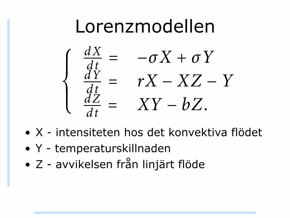
Lorenzmodellen

• Konstruerades av Edward Lorenz på 60-talet för att studera konvektion i atmosfären

• Användes för att argumentera för att kaos existerar i vädersystem

Modellexempel

uppvisade kaos. Utifrån sina observationer myntade han också begreppet �äril-se↵ekten, som sy8ar på just känslighet för förändringar i begynnelsevärden, ochhar sitt ursprung i den retoriska frågan ‘kan en 6ärils vingslag i Brasilien orsakaen orkan i Texas?’⇤�

Lorenz studerade så kallad Rayleigh-Benard-konvektion som uppstår då etttunt lager av vätska hettas från undersidan och kyls av uppifrån (se 5g. ;<). Omtemperaturskillnaden �T T� T⇥ mellan undersidan och ovansidan är liten,så står vätskan stilla och temperaturen varierar jämnt från ovan- till undersidan.Då �T ökar, uppstår så kallade konvenktionsceller där vätskan ömsom stiger,ömsom sjunker i ett cirkulärt mönster. Denna välordnade struktur bryts dockupp om �T ökas ytterligare och ersätts av en turbulent rörelse utan någon somhelst regelbundenhet, och det var detta slags beteende som Lorenz var intresseradav.

T1

T2

Figur ⌥�: Schematisk bild av Rayleigh-Bernard-konvektion. Då ett tunt lagervätska be5nner sig mellan två ytor med en temperaturskillnad �T T� T⇥ kandet om, �T ligger i ett visst intervall, uppstå konvektionsceller.

Systemet liknar åtminstone ytligt det som händer i atmosfären då lu8 värmsupp vid jordytan, stiger uppåt, kyls av och sedan faller ner mot marken igen.Om detta idealiserade modellsystem kan uppvisa kaotiskt beteende – varför dåinte hela atmosfären? Lorenz angrep denna fråga genom att förenkla Rayleigh-Benard–systemet med förhoppningen att det enklare systemet också uppvisardeterministiskt kaos.⇤⇥ Ursprungligen beskrevs den konvekterande vätskan avtvå kopplade partiella di4erentialekvationer: en för riktningen på 7ödet och enför temperaturen. Dessa ekvationer är dock inte lätta att hantera, men genom en

⇤�Lorenz, E. (:?>>).3e Essence of Chaos. CRC Press.⇤⇥Lorenz, E. (:?><). Deterministic non-periodic 7ow, Journal of the atmospheric sciences, ;9,

:<9–:=:.

:99

Rayleigh-Benard konvektion

Lorenzmodellen

• X - intensiteten hos det konvektiva flödet • Y - temperaturskillnaden • Z - avvikelsen från linjärt flöde

Från väder till kaos

smart transformation och några beräkningar kunde Lorenz reducera systemettill tre kopplade ordinära di4erentialekvationer på formen:

dXdt ⌥X ⌥YdYdt rX XZ YdZdt XY bZ .

(98)

Här är X proportionell mot intensiteten hos det konvektiva 6ödet, Y är propor-tionell mot temperaturskillnaden i det uppåt och nedåt strömmande vattnet ochZ är proportionell mot avvikelsen från ett linjärt 6öde. Konstanterna ⌥ , r ochb beror endast på vätskans fysikaliska egenskaper såsom viskositet och termiskkonduktivitet.

Detta ekvationssystem kan tyckas väldigt abstrakt och långt ifrån att beskrivade processer som försiggår i jordens atmosfär, men vi måste hålla i åtanke attLorenz var ute e7er att bevisa att vädersystem kan uppvisa kaotiskt beteende,och om en förenklad leksaksmodell gör det så är det ytterst troligt att det verk-liga systemet också gör det. Och visst hade han rätt, åtminstone vad det gällerleksaksmodellen. Tillståndet hos Lorenzmodellen vid en viss tidpunkt t beskrivsav trippeln X t ,Y t , Z t , och systemets dynamik kan därför avbildas somen bana genom det tredimensionella rummet där riktningen hos banan i varjepunkt bestäms av ekvation (98). Figur :< visar en sådan bana för begynnelsetill-ståndet X � ,Y � , Z � �.⇥, �, � och avslöjar en komplicerade strukturhos dynamiken. Denna struktur brukar kallas för Lorenzattraktorn och kallasför attraktor e7ersom den attraherar banor från alla möjliga begynnelsetillstånd.Detta objekt har rönt stor uppmärksamhet bland matematiker för sina intres-santa egenskaper. Det visar sig bland annat att Lorenzattraktorn är en fraktal.⇥�Modellen uppvisar också den e7erlysta känsligheten i begynnelsevärden och harblivit ett välstuderat typexempel för kaotiska system.

Vi började med väder och vind, och via konvektion landade vi till slut i den rela-tivt enkla Lorenzmodellen som uppvisar komplicerad och till och med fraktaldynamik. Den har de5nitivt ingen prediktiv kra7, men låter oss i stället förklaraen speci5k egenskap hos systemet i fråga, nämligen dess ibland kaotiska beteen-de. Modellen hamnar därför i den bortre änden av det prediktiva–förklarandemodellspektrat: den kan absolut inte hjälpa oss att förutsäga vädret, men i ställetlåta oss förstå dess grundläggande dynamik.

⇥�Tucker, W. (:88:). A Rigorous ODE Solver and Smale’s 9<th Problem. Found. Comp. Math. ::=;–99>.

989

Modellexempel

−20

0

20

40

−40−20

020

40

0

10

20

30

40

50

60

XY

Z

Figur ⌥�: En visualisering av Lorenzattraktorn. BegynnelsetillståndetX � ,Y � , Z � �.⇥, �, � är markerat med en ring i botten av ⇡guren.

�⇢⌧

Lorenzattraktorn

• Fördelar: – Innehållsrik modell – Ger en förståelse för deterministiskt kaos

• Nackdelar: – Ingen prediktion överhuvudtaget – För abstrakt?

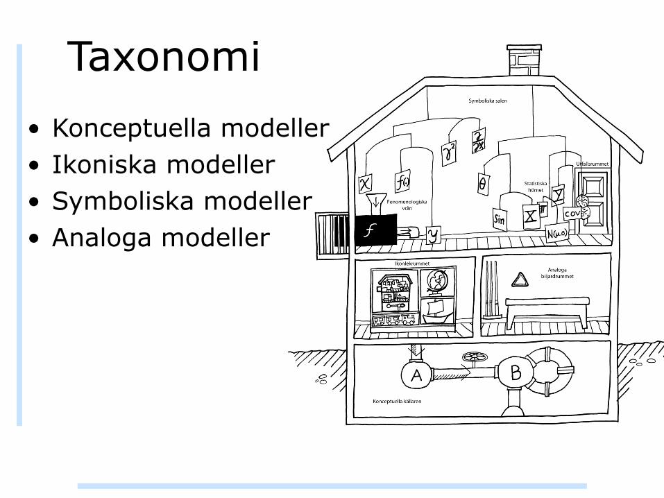
Taxonomi• Konceptuella modeller • Ikoniska modeller • Symboliska modeller • Analoga modeller

Cellers biomekanik• Enskilda cellers mekaniska egenskaper

för viktiga för att förstå blodomloppets egenskaper

Hur deformeras en cell?Modellexempel

and filled with the same salt solution in which the cells were suspended. The micropipette was mountedon a micromanipulator and connected to a pressure regulator (for details see Chien et al., 1978). Withthis pressure regulator it is possible to suddenly apply an aspiration pressure via the micropipette. For anaspiration pressure of - 200 mm H20 the time interval to reach full amplitude is -30-40 ms.

Protocol and Data ReductionThe micropipette was positioned adjacent to the leukocyte. When the aspiration pressure was applied,the leukocyte was drawn towards the pipette tip together with some fluid that entered the pipette. At themoment the leukocyte sealed the pipette, this fluid motion stopped, as could be seen from thedisplacement of adjacent platelets inside or outside of the micropipette.At the moment when the leukocyte made contact with the micropipette it deformed. This deformation

was recorded on the video system, and all measurements were obtained from photographic records of thetelevision monitor made during single frame replay, as shown in Fig. 3. The time between single framesis 16 ms. The displacement of the cell surface into the pipette was measured to the outer edge of thedark interference band of the cell. As shown in Fig. 4 c, if l(t) is the distance from the tip of the pipette tothe tip of the leukocyte tongue inside the pipette, and do the height of the spherical cap of theundeformed cell (Fig. 4 b), then d(t) = I(t) - do is the extent of the deformation of the leukocyte tongueinto the pipette. But d(t) is also equal to the sum of the displacements u'(t) at point A and u'(t) at pointB. Thus, d(t) = | UX(t) + UB(t) (Fig. 4 a). This figure shows the shape of the cell computed accordingto Eq. 10.

FIGURE 4 The shape of the deformed cell. (a) Computed shape and (b,c) actual shape for a cell withequal diameter and pipette size as in a. The displacements d'(t) and d(t) are computed and measured asindicated in the text. Note that the entire cell deforms in this experiment.

SCHMID-SCHONBEIN ET AL. Leukocyte Mechanical Properties 249

the surface of the leukocyte was changed stepwise at time t = 0. After the initial deformation,which is considered to be an elastic response, the cell surface shows a creep displacement thatis nonlinear with time. The continuous line for d(t) in Fig. 5 represents the best possible fit ofthe standard solid model to the experimental data. The best-fit coefficients kl, k2, and ,u arelisted in Fig. 5. The different symbols for d(t) in Fig. 5 represent three experiments measuredat different points on the surface of the same neutrophil. This was achieved by rotating the cellafter each experiment. The close agreement of the three experiments suggests that the cell hasrelatively homogeneous mechanical properties. Similar results were obtained for otherneutrophils, monocytes, and esosinophils.

In general, although leukocytes can undergo large deformation, the current continuum

(a)

[dynl5OO-l-cm2-J 0--

1.0 -

0.9-0.8-0.70.6-

d(t) 0.5[m]0.3-

0.2 -

0.1-

(b)A,P(t) 10001

[dynl]5001rcm;2- 0-

400 dyn/cm2 600 dyn/cm2

0 02 04 Q6 Q8 lo U

K1= 679 dyn/cr,/ K2 1598 dynf/

C ~ ~~~~~~~r: 267 dyn so

0 0.2 0.4 0.6 0.8 1.0 1.2

TIME [s]

900 dyn/cm2| 100 dyn/cm2

0 0.1 Q2 Q3 O Q5 GO 07 08 Q9 1K1 .562 dyn/cm2K2. 1455 dyn/cm2

- 124 dyns/cm2

TIME [sl

FIGURE 7 The aspiration pressure AP(t) and displacement d(t) for a two-step loading experiment (a)and for a loading-unloading experiment (b). The coefficients were computed only from values of d(t)obtained before the second step loading (a) or before the unloading (b). The lines drawn for the secondstep loading (a) and unloading (b) represent predictions without changes of the value of k,, k2, and ,u. Theneutrophils were suspended in the same medium as in Fig. 5.

SCHMID-SCHONBEIN ET AL. Leukocyte Mechanical Properties

ni-v-

I

;M2,cm2

I,CM2

251

Figur ⌥⌥: Den övre bilden visar den experimentella uppställningen där en leuko-cyt utsätts för en spänning med hjälp av undertryck i en mikropipett. Den nedrebilden visar hur förskjutningen varierar med tiden då tryckskillnaden först är<44 dyn/cm� och sedan sänks till 544 dyn/cm� (5 dyn/cm� = 4.5 N/m�). Källa:Schmid-Schönbein, G.W., Sung, K.L., Tözeren, H., Skalak, R. & Chien, S. (5<;5).Passive mechanical properties of human leukocytes. Biophys J. 7:(5): 687–69:.

<;

Viskoelasticitet• Vi tänker oss cellen som ett homogent

viskoelastiskt material • Visköst - som honung så motsätter det

sig deformation • Elastiskt - som ett gummiband uppstår

en återbördande kraft vid deformation • Krypning och relaxation

Den linjära standardmodellen

Modellexempel

krypning), och att om deformationen hålls konstant så minskar spänningen medtiden (detta kallas relaxation).

Dessa egenskaper åter(nns i en mycket enkel modell för viskoelastiska materialsom kallas den ‘linjära standardmodellen’ och som endast består av tre kompo-nenter: två )ädrar och en dämpare (se (g. ,+). Man tänker sig att vänsterdelenav strukturen är förankrad och att den högra sidan utsätts för en dragkra*(spänning) som pekar åt höger. Fjädrarna, som representerar det elastiska hosmaterialet, uppfyller Hookes lag, varför spänningen förändras linjärt med defor-mationen enligt sambandet:

⌃s E⌅s (-)

där E är elasticitetsmodulen, som beskriver styvheten hos materialet. Dämparen,som fångar de viskösa egenskaperna, beter sig enligt:

⌃d ⇧d⌅ddt

(.)

där ⇧ är viskositeten hos dämparen. Detta samband säger att spänningen i däm-paren är proportionellt mot tidsförändringen av deformationen, alltså om defor-mationen är konstant så är spänningen noll.

σ(t)

ε(t)E1

E2

η

Figur �⌥: En schematisk bild av den ’linjära standardmodellen’ för viskoelastiskamaterial. De två )ädrarna med elasticitetsmoduler E� och E⇥ ger uppställningendess elastiska egenskaper medan dämparen har viskositet ⇧. Då konstruktionenutsätts för en tidsberoende spänning ⌃ t svarar den med en förskjutning ⌅ tsom också den beror av tiden.

/-

Modellexempel

and filled with the same salt solution in which the cells were suspended. The micropipette was mountedon a micromanipulator and connected to a pressure regulator (for details see Chien et al., 1978). Withthis pressure regulator it is possible to suddenly apply an aspiration pressure via the micropipette. For anaspiration pressure of - 200 mm H20 the time interval to reach full amplitude is -30-40 ms.

Protocol and Data ReductionThe micropipette was positioned adjacent to the leukocyte. When the aspiration pressure was applied,the leukocyte was drawn towards the pipette tip together with some fluid that entered the pipette. At themoment the leukocyte sealed the pipette, this fluid motion stopped, as could be seen from thedisplacement of adjacent platelets inside or outside of the micropipette.At the moment when the leukocyte made contact with the micropipette it deformed. This deformation

was recorded on the video system, and all measurements were obtained from photographic records of thetelevision monitor made during single frame replay, as shown in Fig. 3. The time between single framesis 16 ms. The displacement of the cell surface into the pipette was measured to the outer edge of thedark interference band of the cell. As shown in Fig. 4 c, if l(t) is the distance from the tip of the pipette tothe tip of the leukocyte tongue inside the pipette, and do the height of the spherical cap of theundeformed cell (Fig. 4 b), then d(t) = I(t) - do is the extent of the deformation of the leukocyte tongueinto the pipette. But d(t) is also equal to the sum of the displacements u'(t) at point A and u'(t) at pointB. Thus, d(t) = | UX(t) + UB(t) (Fig. 4 a). This figure shows the shape of the cell computed accordingto Eq. 10.

FIGURE 4 The shape of the deformed cell. (a) Computed shape and (b,c) actual shape for a cell withequal diameter and pipette size as in a. The displacements d'(t) and d(t) are computed and measured asindicated in the text. Note that the entire cell deforms in this experiment.

SCHMID-SCHONBEIN ET AL. Leukocyte Mechanical Properties 249

the surface of the leukocyte was changed stepwise at time t = 0. After the initial deformation,which is considered to be an elastic response, the cell surface shows a creep displacement thatis nonlinear with time. The continuous line for d(t) in Fig. 5 represents the best possible fit ofthe standard solid model to the experimental data. The best-fit coefficients kl, k2, and ,u arelisted in Fig. 5. The different symbols for d(t) in Fig. 5 represent three experiments measuredat different points on the surface of the same neutrophil. This was achieved by rotating the cellafter each experiment. The close agreement of the three experiments suggests that the cell hasrelatively homogeneous mechanical properties. Similar results were obtained for otherneutrophils, monocytes, and esosinophils.

In general, although leukocytes can undergo large deformation, the current continuum

(a)

[dynl5OO-l-cm2-J 0--

1.0 -

0.9-0.8-0.70.6-

d(t) 0.5[m]0.3-

0.2 -

0.1-

(b)A,P(t) 10001

[dynl]5001rcm;2- 0-

400 dyn/cm2 600 dyn/cm2

0 02 04 Q6 Q8 lo U

K1= 679 dyn/cr,/ K2 1598 dynf/

C ~ ~~~~~~~r: 267 dyn so

0 0.2 0.4 0.6 0.8 1.0 1.2

TIME [s]

900 dyn/cm2| 100 dyn/cm2

0 0.1 Q2 Q3 O Q5 GO 07 08 Q9 1K1 .562 dyn/cm2K2. 1455 dyn/cm2

- 124 dyns/cm2

TIME [sl

FIGURE 7 The aspiration pressure AP(t) and displacement d(t) for a two-step loading experiment (a)and for a loading-unloading experiment (b). The coefficients were computed only from values of d(t)obtained before the second step loading (a) or before the unloading (b). The lines drawn for the secondstep loading (a) and unloading (b) represent predictions without changes of the value of k,, k2, and ,u. Theneutrophils were suspended in the same medium as in Fig. 5.

SCHMID-SCHONBEIN ET AL. Leukocyte Mechanical Properties

ni-v-

I

;M2,cm2

I,CM2

251

Figur ⌥⌥: Den övre bilden visar den experimentella uppställningen där en leuko-cyt utsätts för en spänning med hjälp av undertryck i en mikropipett. Den nedrebilden visar hur förskjutningen varierar med tiden då tryckskillnaden först är<44 dyn/cm� och sedan sänks till 544 dyn/cm� (5 dyn/cm� = 4.5 N/m�). Källa:Schmid-Schönbein, G.W., Sung, K.L., Tözeren, H., Skalak, R. & Chien, S. (5<;5).Passive mechanical properties of human leukocytes. Biophys J. 7:(5): 687–69:.

<;

• Fördelar: – Mekanistisk insikt – Enkel

• Cons: – Begränsad tillämpbarhet – Ingen strukturell likhet

Taxonomi• Konceptuella modeller • Ikoniska modeller • Symboliska modeller • Analoga modeller • Fenomenologiska

modeller

Modeller för vattenavrinning• Hydrologiska processer är ofta komplexa

och spänner över flera rums- och tidsskalor

• Prediktion av vattenflöde har stor samhällsnytta

Neurala nätverk• Inspirationen kommer från

biologiska neurala nätverk, tex. hjärnor

• Ett effektivt verktyg för att förutsäga utfallet hos komplexa system (och klassificering)

• Består av artificiella neuroner som är sammanlänkade i ett nätverk

Modeller för vattenavrinning

på multilagers perceptronen (MLP). Den består av en uppsättning noder, ellerneuroner, som i likhet med neuroner i våra hjärnor, är kopplade till varandra.Varje nod tar emot signaler från en uppsättning noder och kan också sända i vägsignaler. Dessa kan vara av två huvudslag: antingen stimulerande eller dämpande,men kan också ha olika intensitet. I likhet med riktiga neuroner så tänker mansig att en nod endast sänder i väg signaler, eller ‘fyras av’, då den blivit stimuleradöver en viss tröskel. Om en nod får insignaler från 1era andra noder så summerasdessa inuti noden, med konventionen att dämpande signaler är negativa ochstimulerande positiva. Matematiskt kan vi formulera detta som att tillståndethos en nod i i nätverket ges av

x i fjWi jx j ⌥ i (4)

där f x tanh x är en så kallad överföringsfunktion, W är en matris ellertabell som beskriver kopplingarnamellan noderna och ⌥ i nodens interna tröskel-värde. Förenklat kan vi säga att nodens värde ges av den viktade summan av denoder den är kopplad till, matad genom överföringsfunktionen f x . Denna ärutritad i 0gur 34 och visar att noden beter sig som vi beskrev ovan; bara om dentotala stimulansen överstiger det interna tröskelvärdet är noden aktiv (x i ⇧),annars är den inaktiv (x i ⇧).

MatrisenW beskriver alltså hur noderna är sammanlänkade. I MLP-nätverketär noderna organiserade i distinkta lager: ett in-lager, ett eller 1era gömda lageroch ett ut-lager (se 0g. 35). Noderna i in-lagret svarar mot variabler vi kännertill, medan noderna i ut-lagret svarar mot dem som ska predikteras. Nätverketfungerar så att indata presenteras vid in-lagret. Med hjälp av ekvation (4) så upp-dateras nodvärdena först i de gömda lagren och sist i ut-lagret. Värdena på dessanoder svarar mot nätverkets förutsägelse, och på grund av denna struktur brukardessa nätverk också kallas ‘framåt-kopplade’ (feed-forward) neurala nätverk, därinformationen matas från ena sidan av nätverket till den andra.

Men hur bestäms egentligen kopplingskonstanternaW , som faktiskt är de somgör hela jobbet? Dessa fastställs genom att nätverket tränas på kända par av in-och utdata som uppvisar de mönster nätverket senare förväntas känna igen. Förstinitieras ett nätverk där vikterna iW valts helt slumpmässigt, och sedan matasträningsparen in i nätverket i tur och ordning. För varje indata gör nätverketen prediktion P , och e2ersom den riktiga utdatan P är känd kan vi räkna utprediktionsfelet E P P . Med hjälp av detta felet så uppdateras vikterna påett sådant sätt att nätverket bättre och bättre på att förutsäga utdatan.⇥�

För att återgå till exemplet med sambandet mellan nederbörd och 1öde, så har⇥�En vanligmetod för att åstadkommadetta är så kallad ‘backpropagation’ somuppdaterar vikterna

i de olika lagerna sekventiellt på ett sätt som i varje steg ämnar att minimera felet.

76

−1

−0.8

−0.6

−0.4

−0.2

0

0.2

0.4

0.6

0.8

1

total activation

θithe

stat

e of

nod

e x i

In-layer Hidden layer Out-layerKn

own

varia

bles

Varia

bles

to b

e pr

edict

ed

Tillämpning• Nätverkets dynamik beror på vikter W

som justeras genom att träna nätverket • Indata är nederbörd och flöde vid flera

tidpunkter och utdata är det framtida flödet på en specifik plats

Modellexempel

NEURAL NETWORK MODELS FOR HYDROLOGIC PREDICTIONS AT MULTIPLE STATIONS

Time(days)0 200 400 600 800

0

5

10

15

20

25Observed flowPredicted flow

Station 1

Time(days)0 200 400 600 800

MLP

flow

(m

3 /s)

0

5

10

15

20

25Observed flowPredicted flow

Training Testing

Station 2 Station 2

Time(days)0 200 400 600 800

MLP

flow

(m

3 /s)

0

5

10

15

20

25Observed flowPredicted flow

Training Testing Training Testing

Time(days)

0 200 400 600 800

MLP

flow

(m

3 /s)

0

5

10

15

20

30

25 Observed flowPredicted flow

Station 3

Training Testing

Time(days)

200 400 600 8000

Observed flowPredicted flow

0

5

10

15

20

30

25

Station 4

Training Testing

Time(days)

0 200 400 600 800

MLP

flow

(m

3 /s)

0

5

10

15

20

30

25

Observed flowPredicted flow

Station 4

Training Testing

Time(days)

0 200 400 600 800

RB

FN

N fl

ow (

m3 /

s)R

BF

NN

flow

(m

3 /s)

RB

FN

N fl

ow (

m3 /

s)R

BF

NN

flow

(m

3 /s)

0

5

10

15

20

25Observed flowPredicted flow

Station 1

Training Testing

Time(days)

0 200 400 600 800

Observed flowPredicted flow

Station 3

Training Testing

0

5

10

15

20

30

25

Figure 10. Hydrographs of time versus flow during training and testing for the four stations

3 for all stations for both MLP and RBFNN models.Scatter plots between measured and predicted flow dataserve as a useful visual aid to assess a model’s accuracy.The closer the scatter points are to the line of thebest fit, the better the model. Figure 9 shows that theMLP models had smaller scatter around the best fitline than the RBFNN models for all four gaugingstations. Figure 10 shows the corresponding hydrographsfor the four stations during training and testing. These

plots, when combined with results shown in Table II,indicate that model performance for the full range offlow data evaluated in this study was superior for theMLP model, as indicated by greater R2 and CE andlower RMSE values compared with those for the RBFNNmodel. Both models underpredicted high flow eventsand over predicted low flow events at some of thegauging stations (Figures 9 and 10). The cause of thesediscrepancies needs to be further evaluated to improve

Copyright © 2008 John Wiley & Sons, Ltd. Hydrol. Process. (2008)DOI: 10.1002/hyp

Figur ⌥�: Prediktion av -öde med hjälp av ett neuralt nätverk. Källa: Mutlu, E.,Chaubey, I., Hexmoor, H. & Bajwa, S.G. (0..4). Comparison of arti,cial neuralnetwork models for hydrologic predictions at multiple gauging stations in anagricultural watershed. Hydrological Processes, 00:1.53-1/.2.

5.

• Fördelar: – Inga förståelse för mekanismer är nödvändig – Beräkningsmässigt effektivt

• Nackdelar: – Endast prediktion ingen förståelse – Ingen teori för neurala nätverk existerar – Risk för över-träning

Taxonomi• Konceptuella modeller • Ikoniska modeller • Symboliska modeller • Analoga modeller • Fenomenologiska

modeller • Statistiska modeller

Statistisk modell för genuttryck i hjärntumörer

Bansal et al, 2007; Bonneau et al, 2007; Lehar et al, 2007;Nelander et al, 2008; Lauria et al, 2009). A third alternative isto use the naturally occurring genetic variation in a separatingpopulation to study the relationship between genotype andexpression phenotype (Jansen, 2003; Lee et al, 2006, 2009;Rockman, 2008; Suthram et al, 2008; Zhu et al, 2008; see alsoDiscussion). Here, we focus on the role of acquired geneticvariations in tumors, specifically CNAs, and ask how thesecan be used to derive transcriptional networks. CNAs areprevalent in several human cancers, and tend to appear in apatient-specific and multifactorial manner in the tumors,which resembles an optimal experimental design to derivecausality (Fisher, 1926).We present a global model of CNA-driven transcription

in the brain tumor glioblastoma. The model is derived usingEPoC (Endogenous Perturbation analysis of Cancer), acomputational method that constructs network models ofmRNA expression, viewing CNAs as informative systemperturbations introduced endogenously during the evolutionof the tumor, and the corresponding mRNA profiles as thesteady-state response to that perturbation. We apply EPoC toglioblastoma data from The Cancer Genome Atlas (TCGA)consortium. Previous analyses of glioblastoma have revealedaltered pathways and disease subtypes (Pollack et al, 2002;Freije et al, 2004; Phillips et al, 2006; Tso et al, 2006; Lee et al,2008; TCGA-Consortium, 2008; Dahlback et al, 2009; Verhaaket al, 2010; Cerami et al, 2010) and networks of correlatingtranscripts (Carro et al, 2010) (ARACNE). Key examplesof CNA/mRNA analyses for other tumors include clusteringand modular network modeling, leading to the discoveryof regulators such as MITF, RAB27A and TBC1D16 inmalignant melanoma (Garraway et al, 2005; Akavia et al,2010), and linkage analysis to reveal the association of cMYCamplification to wound healing signatures in breast cancer(Adler et al, 2006). Network analysis of 654 selected breastcancer transcripts and 384 genomic regions has identified acandidate regulatory region on chromosome 17 (Peng et al,2008). Canonical correlation analysis (CCA) has also beenput forth as an alternative non-network approach to inte-grating DNA/mRNA data (Waaijenborg et al, 2008; Wittenet al, 2009).We use EPoC to construct a gene-level model, which

encompasses 10 672 genes, causally connecting CNAs toexpression changes in glioblastoma. First, we establish thatthe parameters of the EPoC network model can be robustlyestimated from paired genome-wide DNA- and RNA-leveldata from a set of tumors, using a combination of lassoregression and bootstrap. Second, we show that a novelscore, based on a sparse singular value decomposition ofthe derived CNA–mRNA network model, identifies prognosticbiomarkers capable of clinical stratification into short-termand long-term survivors. Third, EPoC identifies key mecha-nisms (disease-driving CNAs), which we assess by chemo-informatic analyses and comparisons to known biologicalpathways, revealing the likely existence of short regulatorypaths between EPoC hubs and targets, as well as 15 candidatedrug targets. We confirm a candidate hub, the p53-interactingprotein Necdin, NDN, in U87MG, U373MG, U343MG andT98 glioma-derived cell lines by experimentally testing asmall transcriptional network around NDN, receptor tyrosine

kinases EGF receptor (EGFR) and platelet-derived growthfactor receptor alpha (PDGFRA). Finally, we demonstraterapid and consistent performance of EPoC in comparisonwith mRNA-only methods, standard expression quantitativelocus (eQTL) methods and two recent multivariate methodsfor genotype–mRNA coupling (Peng et al, 2008; Lee et al,2009).

Results

Modeling copy number-dependent transcriptionin tumors

Transcriptional and CNA-driven networksTo connect mRNA levels with DNA copy number inglioblastoma tumors, we adapt a common model for mRNAtranscription regulation and turnover. Thismodel formulation,related to the so-called S-system (Savageau, 1969, 1976;Crampin et al, 2004), takes the form of sets of differentialequations:

dyidt

¼ uiaiYn

j¼1

ywij

j

zfflfflfflfflfflfflffl}|fflfflfflfflfflfflffl{synthesis

" biYn

j¼1

yvijj

zfflfflfflfflffl}|fflfflfflfflffl{decay

; i ¼ 1; . . . ;n; ð1Þ

where n is the number of genes, dyi/dt and yi, i¼1,2,y,ndenote the change rate and average mRNA concentrations ina tumor respectively, and uiX0, i¼1,2,y,n the averagenumber of gene copies corresponding to a particular transcript(Figure 1B). Equation (1) states that the change rate oftranscript yi is the difference between its synthesis rate and itsdecay rate. The synthesis rate is determined by the number ofcopies of the gene’s DNA, ui, the regulatory effects of othergenes, wij and a gene-specific synthesis constant, ai. Similarly,the decay rate is determined by the regulatory effects of othergenes, vij and a gene-specific decay constant, bi. Obviously, theassumption of proportionality on ui is a simplification andunlikely to hold for all genes in the genome (e.g., gene copiesmay generate transcripts at different rates due to epigeneticdifferences). Nevertheless, recent data indicate that it is areasonable approximation for a large proportion of genes inthe genome (Nilsson et al, 2008).The procedure used to estimate the model parameters in

Equation (1) is described in detail in Materials and methods.In short, assuming steady-state conditions, the log-transformedand zero-centered mRNA and CNA profiles of glioblastoma canbe summarized by two mutually complementing linearsystems. The first of these represents the transcriptionalnetwork (A):

ADY þ DU þ R ¼ 0; ð2Þ

where DY and DU are stack matrices of log-transformed andzero-centered mRNA and CNA profiles of glioblastoma,respectively, and R (defined by the a’s and b’s of the originalmodel, Materials and methods) is a matrix that captures theeffects on transcription of non-CNA perturbations in individualtumors (e.g., SNPs, sequence mutations or environmentaleffects). The transcriptional network A¼{aij} relates to theoriginal model by aij¼wij"vij, meaning its elements aij

Network modeling of glioblastomaR Jornsten et al

2 Molecular Systems Biology 2011 & 2011 EMBO and Macmillan Publishers Limited

Figure 1 Overview of the EPoC modeling framework. (A) Using genome-wide, paired mRNA- and DNA-level data as input, EPoC generates a quantitativecausal network model of the global effects of copy number aberrations on mRNA expression. The resulting model is subsequently used to predict disease-drivinggenes and prognostic indicators. (B) EPoC is based on systems of differential equations that take into account that the transcription of a gene is determined bothby its own DNA copy number (straight arrows) and the product of other genes (bent arrows). (C) Our method generates two mutually complementary networksdenoted as A and G. The A network captures transcript–transcript interactions (left), whereas the G network contains the direct and indirect effects of CNA pertur-bations on transcription (middle). The singular value decomposition of G can be used to identify the CNAs whose perturbations are maximally amplified by thenetwork (i.e., they have a strong overall transcriptional effect; yellow nodes), and the mRNA transcripts whose expression are most altered by these perturbations(green nodes; right panel).

Network modeling of glioblastomaR Jornsten et al

& 2011 EMBO and Macmillan Publishers Limited Molecular Systems Biology 2011 3

Modell för genuttryck:

Jörnsten et al. 2011

• Fördelar: – Beräkningseffektivt – ?

• Nackdelar: – Endast prediktion ingen förståelse – Dålig noggranhet

Begriplighet och prediktionskraft

Komplexitet

Prediktion

skraft

Begriplighet

Komplexitet

AnvändbarhetA B

Prediktionskraft

Begriplighet

I

II III

IV

AB

C

Problemlösning enligt Polya

1. Förstå problemet 2. Tänk ut en plan 3. Genomför planen 4. Betrakta lösningen

Förstå problemet

• Vad är det som efterfrågas? • Kan du formulera problemet med egna

ord? • Har du tillräckligt med data för att lösa

problemet? • Förstår du alla definitioner?

Tänk ut en plan

• Rita en bild • Bestäm notation • Kan du identifiera delproblem? • Finns det några symmetrier? • Har du löst ett liknande problem förut? • Finns det någon modell/ekvation du kan

använda?

Genomför planen

• Bra planering gör detta steg kortare • Kontrollera varje steg i lösningen

Betrakta lösningen

• Är lösningen rimlig? (testa med extrema värden på parametrar)

• Finns det några andra sätt att lösa problemet?

• Förstår du lösningen intuitivt? • Kan metoden användas för att lösa

liknande problem?

Modellering enligt Giordano

1. Identifiera problemet 2. Gör antaganden

1. Identifiera och klassificera variabler 2. Bestäm förhållandet mellan variabler

3. Lös modellen 4. Verifiera lösningen

1. Löser den problemet 2. Är den rimlig? 3. Testa den med verklig data

5. Implementera modellen

Fenomen, teori och modell

Theory, model and phenomena

Teori

Modell

Fenomen

Experiment

Rådata

Data

Databehandling

Validering

Grundläggande

principer

Ideér till

nya teorierObservation

Datainsamling

Konkretisering

Definition ochbegränsning

• Korrekt

• Fullständig

• Generell

• Enkel

• Korrekt eller felaktig

• Ofullständig

• Specifik

• Enkel eller komplicerad

⇔

⇔

⇔

⇔

Teori eller modell• Model från teori eller teori från modell?

En model av vad?

• Ett fenomen kan både vara specifikt och abstrakt

• Modeller av modeller av modeller… • Arketypiska modeller (Lorenz-modellen) • Strukturell likhet mellan modell och

fenomen (isomorfism) • Positiva och negativa analogier

Validering av modeller• Modeller jämförs ofta med experimentell

data • Vilken slags noggrannhet kan vi förvänta

oss? (kontextberoende) • Kvalitativ och kvantitativ validering

We did not dispose of double measurements for the breasttumor data and the error analysis was performed using the lungtumor data set only. However, the same error model was appliedto the breast tumor data, as both relied upon the samemeasurement technique.

This result allowed quantification of the measurement errorinherent to our data and was an important step in the assessmentof each model’s descriptive power.

Descriptive powerWe tested all the models for their descriptive power and

quantified their respective goodness of fit, according to variouscriteria. Two distinct estimation procedures were employed. Thefirst fitted each animal’s growth curve individually (minimizationof weighted least squares, with weights defined from the errormodel of the previous section, see Material and Methods). Thesecond method used a population approach and fitted all thegrowth curves together. Results are reported in Figure 2 andTables 1 and 2. Parameter values resulting from the fits arereported in Tables 3 and 4.

Figure 2A depicts the representative fit of a given animal’sgrowth curve for each data set using the individual approach.From visual examination, the exponential 1 (1), logistic (2) andexponential-linear (1) models did not well explain lung tumorgrowth and the exponential 1 (1) and logistic (2) models did notsatisfactorily fit the breast tumor growth data. The other models

seemed able to describe tumor growth in a reasonably accuratefashion.

These results were further confirmed by global quantificationsover the total population, such as by residuals analysis (Figure 2C)and global metrics reported in Tables 1 and 2. When consideringgoodness-of-fit only, i.e. looking at the minimal least squared

errors possibly reached by a model to fit the data (metric1

Ix2 in

Tables 1 and 2), the generalized logistic model (3) exhibited thebest results for both data sets (first column in Tables 1 and 2). Thisindicated a high structural flexibility that allowed this model toadapt to each growth curve and provided accurate fits. On theother hand, the exponential 1 (1) and logistic (2) models clearlyexhibited poor fits to the data, a result confirmed by almost all themetrics (with the exception of the AICc).

Influence of the goodness-of-fit metric. Being able toclosely match the data is not the only relevant criterion to quantifythe descriptive power of a model since parameter parsimony of themodel should also be taken into account. Other metrics wereemployed that balanced pure goodness-of-fit and the number ofparameters (see Materials and Methods for their definitions).Among them, AICc exhibited the strongest penalization for a largenumber of parameters. However, this metric was in multipleinstances in disagreement with the other metrics dealing withparsimony. For this reason, we also reported the values of AIC.These were found globally in accordance with the RMSE. The

Figure 2. Descriptive power of the models for lung and breast tumor data. A. Representative examples of all growth models fitting thesame growth curve (animal 10 for lung, animal 14 for breast). Error bars correspond to the standard deviation of the a priori estimate of measurementerror. In the lung setting, curves of the Gompertz, power law, dynamic CC and von Bertalanffy models are visually indistinguishable. B. Correspondingrelative growth rate curves. Curves for von Bertalanffy and power law are identical in the lung setting. C. Residuals distributions, in ascending order ofmean RMSE (13) over all animals. Residuals (see formula (15) for their definition) include fits over all the animals and all the time points.Exp1 = exponential 1, Exp-L = exponential-linear, Exp V0 = exponential V0, Log = logistic, GLog = generalized logistic, PL = power law, Gomp = Gom-pertz, VonBert = von Bertalanffy, DynCC = dynamic CC.doi:10.1371/journal.pcbi.1003800.g002

Description and Prediction of Tumor Growth

PLOS Computational Biology | www.ploscompbiol.org 7 August 2014 | Volume 10 | Issue 8 | e1003800

Sammanfattning

• Taxonomi • Problemlösning • Fenomen, teori

och modell