Modeling Wind Energy Resources in Generation Expansion Models

Vladimir KORITAROVCenter for Energy, Environmental, and Economic Systems AnalysisDecision and Information Sciences Division (DIS)ARGONNE NATIONAL LABORATORY9700 South Cass Avenue, DIS-221Argonne, IL 60439Tel: 630-252-6711Email: Koritarov@anl.gov

FERC Technical Conference on Planning Models and Software

Washington, DCJune 9-10, 2010

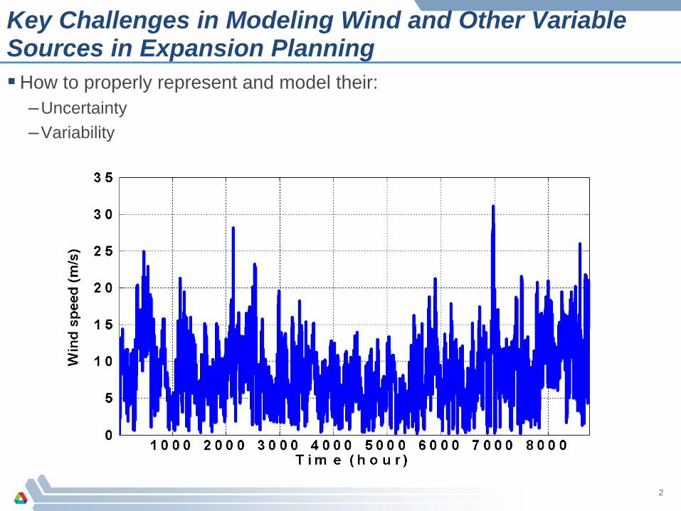
Key Challenges in Modeling Wind and Other Variable Sources in Expansion Planning

How to properly represent and model their:–Uncertainty–Variability

2

Wind Plant Characterization

3

Wind speed (m/s) Power (kW)0 03 21.94 75.15 155.86 274.37 439.38 6689 932.110 1215.411 1418.212 1473.713 1496.514 150015 150016 150017 150018 150019 150020 150021 150022 1500

Cut‐in wind speed: 3.0 m/sCut‐out wind speed: 22 m/s

Example: Wind Turbine Vensys 77 (1.5 MW)

Power Curve

Wind Speed Characterization

4

Date Hour 70m Wind speed mph1‐Sep‐06 0 7.10

1 8.102 6.783 7.374 6.475 6.836 8.827 9.128 8.409 7.75

10 9.9011 8.1212 10.6313 10.9214 11.3215 10.4216 13.2717 11.4818 12.1219 11.5520 12.4821 11.8222 11.0523 9.22

Historical Wind Speed: Wind Speed Models:

Weibull Distribution

Time Series

Markov Chains, etc.

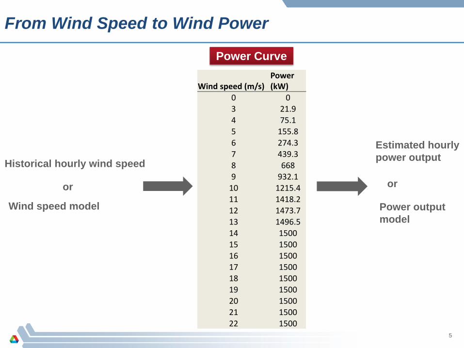
From Wind Speed to Wind Power

5

Wind speed (m/s)Power (kW)

0 03 21.94 75.15 155.86 274.37 439.38 6689 932.110 1215.411 1418.212 1473.713 1496.514 150015 150016 150017 150018 150019 150020 150021 150022 1500

Historical hourly wind speed

Estimated hourlypower output

or

Wind speed model Power outputmodel

or

Power Curve

What is the Capacity Value of a Wind Plant?

Utilities use different approaches to estimate the capacity value (capacity credit or firm power) of wind plantsFirst we need to distinguish whether capacity credit is determined for planning or operation purposes:

Long-Term Expansion Planning:–The long-term capacity credit is usually linked to how much of new conventional

generating capacity additions can be replaced by the wind plant–The overall availability of wind plant (e.g., capacity factor) is one of the key factors

influencing the capacity value of wind plant in the long term

Operations Planning:– In operations planning, the capacity credit is related to how much wind capacity will

be available for meeting the load next day, especially during the peak hours–Good wind forecasting plays a key role in determining the wind capacity credit in the

short term

6

Wind Capacity Credit and System Reliability

Reliability of system operation is one of important aspects for determining both short- and long-term capacity creditsAlthough the operational availability of a wind turbine may be very high, it will not operate when there is no wind, which makes it a relatively unreliable generation sourceThe concept of Equivalent Load-Carrying Capacity (ELCC) is often used to determine the capacity credit of wind farms in the long termThe ELCC method is based on the LOLP measure of system reliability so that a wind farm is benchmarked against an ideal, perfectly reliable unit with 100% availabilityThe amount of perfectly reliable capacity that achieves the same system reliability as in the case with wind plant determines the ELCC of a wind plant A related “equivalent capacity” approach is to use an alternative conventional unit (e.g., gas turbine) instead of the ideal unit The equivalent unit is sized so that the system LOLP is the same if calculated with a wind plant instead of the gas plant

7

8

ELCC Decreases with Higher Penetration of Wind Capacity in the System

German utility E.ON: “The more wind power capacity is on the grid, the lower the percentage of traditional generation it can replace.”–Firm capacity from wind in 2007:

about 7% of installed capacity–Firm capacity in 2020 is expected to

drop to 4%.

Source: E.ON Wind Report 2005

Benefits of Wind Power

9

Energy Credits• Energy generation + fuel savings

Capacity Credits• Capacity value or ELCC

Emission Credits• Reduced overall pollutant emissions

in the system

Calculation of Wind Power Benefits in the Long Term

Economic cost/benefit analysis

Usually performed over the lifetime of a wind farm

Calculations performed in terms of net present value

Long-Term Benefits of Wind Power Can Be Calculated using Capacity Expansion Models

The objective of models for optimal capacity expansion, such as WASP-IV, is to determine the least-cost system expansion plan that would meet the demand over the study period, while satisfying all reliability and other constraints specified by user

The operating and investment costs, determined by the model, can be used to calculate energy and capacity credits of wind plants

The emissions of various pollutants calculated by the model can be used to determine the emission credits

Calculation of Long-Term Benefits of Wind Power using a Capacity Expansion Model

Typically, the analysis is performed for two scenarios:–Case without wind power (Reference Case)–Case with the wind power capacity

System reliability (e.g., LOLP and ENS) should be kept at approximately the same level in both scenarios

The analysis can be performed either for a specific wind farm or for a given penetration of wind farm capacity over the study period

Comparison of Results for Two Scenarios

Energy credits can be calculated from the differences in operating costs

Capacity credits can be calculated from the differences in expansion schedules:–The amount of conventional capacity (MW) displaced or deferred by wind

farms–Savings in the investment costs ($) for new generating capacity can also

be calculated

Emission credits can be calculated from the differences in air emissions

Representation of Wind Power in Capacity Expansion Models

There are several approaches for modeling wind power in expansion planning models:

1. Load Modification Approach (“Negative Load” approach)

2. Supply-Side Approach (wind is treated as conventional power plant)i. Run-of-river hydro capacityii. Unreliable thermal capacity

3. Multi-Block Probabilistic Simulation Approach

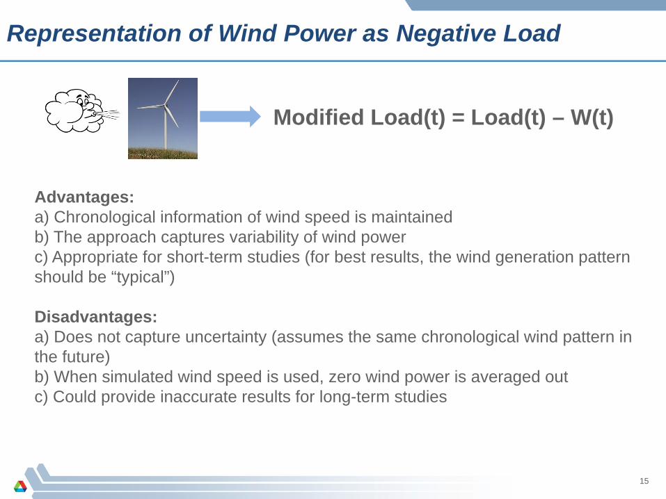
Representation of Wind Power as Negative Load

15

Advantages:a) Chronological information of wind speed is maintainedb) The approach captures variability of wind powerc) Appropriate for short-term studies (for best results, the wind generation pattern should be “typical”)

Disadvantages:a) Does not capture uncertainty (assumes the same chronological wind pattern in the future)b) When simulated wind speed is used, zero wind power is averaged outc) Could provide inaccurate results for long-term studies

Modified Load(t) = Load(t) – W(t)

Supply-Side Approach

16

Advantages:a) Wind power is treated as conventional run-of-river hydro or unreliable thermal power plant b) The wind plant is used in dispatch simulations and reliability calculationsc) The approach captures some variability and some uncertaintyd) Appropriate for long-term studies

Disadvantages:a) Stochastic nature of wind power (zero-rated capacity) is misrepresentedb) Chronological hourly wind information is not captured (not a concern for long-term studies)

Available plant generation = Wind generation

Supply-Side Approach: Representation of Wind Power as Run-of-River Hydro Plant

Wind generation has some similarities with run-of-river hydro generation:–Both are non-dispatchable (power has to be used when produced)–Both can have seasonal variations–Both are characterized by a level of uncertainty (wind conditions or

hydrological conditions)–There is practically no energy storage available

If a capacity expansion model allows for multiple hydrological conditions, these can also be used to express the probabilities of expected wind generation

Using the modeling of run-of-river hydro, specify the expected wind generation and available capacity by period, according to their probabilities of occurrence

Both existing and candidate wind plants can be represented

Supply-Side Approach: Representation of Wind Power as Unreliable Thermal Generating Capacity

Simple and easy approach, both existing and candidate wind farms can be represented

Wind farm is represented as very unreliable thermal generating unit

The forced outage rate of the thermal unit should be specified high (thermal unit generation should match the expected generation from the wind farm)

Since wind farms operate throughout the year, there should be no maintenance requirements for the fictitious thermal unit

Fuel costs can be specified as zero, while O&M costs should correspond to the real O&M costs of the wind farm

Since the running costs of this unit are very low or zero, the wind farm will always be loaded when available

18

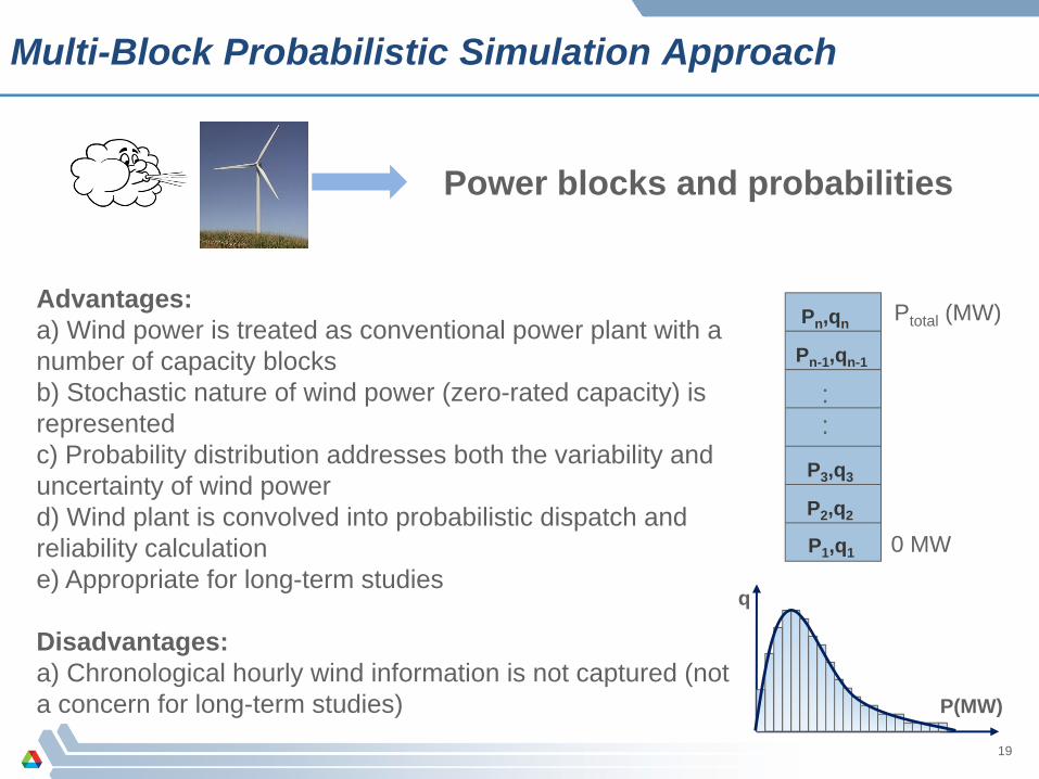
Multi-Block Probabilistic Simulation Approach

19

Advantages:a) Wind power is treated as conventional power plant with a number of capacity blocksb) Stochastic nature of wind power (zero-rated capacity) is representedc) Probability distribution addresses both the variability and uncertainty of wind powerd) Wind plant is convolved into probabilistic dispatch and reliability calculatione) Appropriate for long-term studies

Disadvantages:a) Chronological hourly wind information is not captured (not a concern for long-term studies)

Power blocks and probabilities

0 MW

Pn,qn

Pn-1,qn-1

P2,q2

P1,q1

P3,q3

Ptotal (MW)

::

q

P(MW)

Implementation of Multi-Block Approach

Wind speed (m/s)

Power Output Curve

0 MW

Pn,qn

Pn-1,qn-1

P2,q2

P1,q1

P3,q3

Ptotal (MW)

PROBABILISTICDISPATCH

Wind Power Output (MW)

Blocks & Probabilities

::

q

P(MW)

Wind power (MW)

n Range Average Value Probability0 0 0 0.01431 0-60 30 0.16522 60-120 90 0.07563 120-180 150 0.08214 180-240 210 0.07925 240-300 270 0.07926 300-360 330 0.10477 360-420 390 0.11908 420-480 450 0.09869 480-540 510 0.094610 540-600 570 0.0875

Mean = 284.1St. dev. = 182.1

Mean = 285.5St. dev. = 181.2

Wind Capacity Blocks and Their Probabilities Can Be Determined using a Wind Power Stochastic Model

Blocks & Probabilities

Data Processing for Multi-Block Approach

22

Date Hour70m Wind speed 

(m/s)1‐Sep‐06 0 7.10

1 8.102 6.783 7.374 2.475 1.836 8.827 9.128 8.409 7.7510 9.9011 8.1212 10.6313 10.9214 11.3215 10.4216 13.2717 11.4818 12.1219 11.5520 12.4821 11.8222 11.0523 9.22

Wind speed (m/s) Power kW0 03 21.94 75.15 155.86 274.37 439.38 6689 932.110 1215.411 1418.212 1473.713 1496.514 150015 150016 150017 150018 150019 150020 150021 150022 1500

BlockPower Output Probability

0 0 0.13061 0.6 0.12042 1.2 0.20563 1.8 0.11944 2.4 0.02785 3 0.10426 3.6 0.06027 4.2 0.10008 4.8 0.01679 5.4 0.030610 6 0.0847

Wind Farm (6 MW)

Example:Wind speed (m/s) Power Output Curve

q

P(MW)

Blocks & Probabilities

Wind Farm 1

Wind Farm 2

Wind Power Aggregation

WIND FARM AGGREGATION

0 MW

Pn,qn

Pn-1,qn-1

P2,q2

P1,q1

P3,q3

Ptotal (MW)

::

Total Output (MW)

Wind Farm Correlation

Correlation in wind farm power output is decreasing with the distance between the wind farmsIn the US, correlation factors are different for N-S and E-W directions

24

Source: NREL