Modeling the Performance of the Standard Cirrus Glider

Modeling the Performance of the Standard Cirrus Glider using Navier-Stokes CFD

Thomas HansenNorwegian University of Science and Technology

N-7491, NTNU Trondheim, Norwayt❤♦♠❛s✳❤✳❤❛♥s❡♥❅♥t♥✉✳♥♦

Abstract

The performance of the Standard Cirrus glider is simulated using a Computational Fluid Dynamics code, solving theincompressible Navier-Stokes equations for steady flow. Tocalculate the transitional boundary layer flow a correlation-based transition model is used. It is found that the numerical model is able to predict the performance of the StandardCirrus well. The simulations using the transition model arefound to improve the results compared to fully turbulentsimulations, except for the region of the stall. The best in-flight measured glide ratio for the Standard Cirrus is 36.5 at94.5 km/h. The simulations using the transition model predict a best glide ratio of 38.5 at 95 km/h.

IntroductionThe development of modern computer tools has led to a revolution

in the design and construction of high-performance gliders. Today,the aerodynamic and the structural potential of new designscan beinvestigated and refined using computers to produce gliderswith per-formance and handling qualities inconceivable just a few decades ago.The JS1, ASG29 and the Diana 2 are examples of modern gliders de-veloped by using the latest computational tools in combination withexperience and experimental testing. Glide ratios above 50:1 and max-imum speeds higher than 280 km/h are today normal for glidershav-ing 15 and 18 meter of wing span. However, modern numerical toolsstand in sharp contrast to the methods applied for the designof the firsthigh-performance gliders. Some 30 years ago the tools available con-sisted almost entirely of analytic approximation methods,wind tunnelexperiments and flight testing. The materials and the accuracy of theproduction methods available at the time were also limitingfactors inthe quest to develop high-performance gliders.

In this paper, the Standard Cirrus glider is simulated by solving theReynolds-Averaged Navier-Stokes (RANS) equations in the commer-cial computational fluid dynamics (CFD) software STAR-CCM+[1].The main purpose of the study is to create a validated reference modelfor the performance of the glider in steady level flight. To predict theimportant boundary layer flows, the correlation-basedγ–Reθ transitionmodel is used [2,3]. The results obtained in this work shouldenable fu-ture investigations regarding possible performance and handling qualityenhancements for the glider. The design of new winglets, theinstalla-tion of an electrical engine and research on new turbulator technologyare examples of studies that could benefit from using a validated RANSmodel. The model of the Standard Cirrus is also intended to bea refer-ence model for investigating and refining the results from other numer-ical simulation tools. The abilities and limitations of less computation-ally expensive tools such as lifting line methods, vortex-lattice codes,and potential flow solvers can all be evaluated better by comparing theresults to a validated Navier-Stokes model.

To perform the simulations, the geometry of the specific StandardCirrus named LN-GTH is first measured using a digitizing arm and asurface model is created. Then, the performance of the airfoil used atthe outer part of the Cirrus wing is analyzed using a two dimensional

Fig. 1: The Standard Cirrus. Lennart Batenburg, with permission

mesh. The simulations are performed to investigate the accuracy of theγ–Reθ transition model in detail. The two dimensional computationsare validated by comparing the results to experimental values from thelow-turbulence pressure wind tunnel at NASA Langley. Finally, thethree dimensional model of the Standard Cirrus is simulatedin steadylevel flight for velocities from 90 km/h to 160 km/h. The threedimen-sional CFD simulations are validated by comparing the results to flighttests performed with a Standard Cirrus at the Idaflieg summermeetingin 2011.

The Standard CirrusThe Standard Cirrus (Fig. 1) was designed by Dipl.-Ing. Klaus

Holighaus at the Schempp-Hirth factory and flew for the first time inMarch 1969. The glider is a 15-m design without flaps and was orig-inally built to compete in the Standard Class. The glider uses an all-moving tailplane, is equipped with air brakes on the upper surface ofthe wings, and can carry 80 kg of water ballast to increase theflightperformance. The wing of the glider is designed using two differentairfoils, where the root airfoil blends linearly into the airfoil that is used

VOL. 38, NO. 1 January–March 2014 5 TECHNICAL SOARING

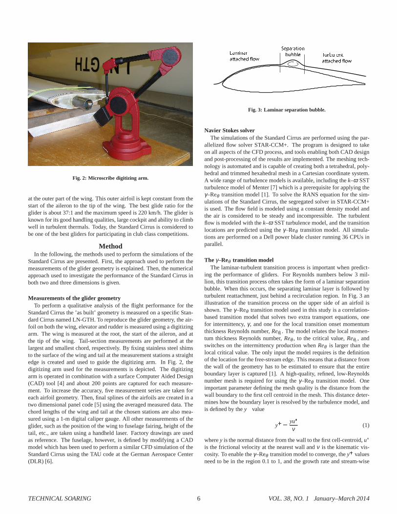
Fig. 2: Microscribe digitizing arm.

at the outer part of the wing. This outer airfoil is kept constant from thestart of the aileron to the tip of the wing. The best glide ratio for theglider is about 37:1 and the maximum speed is 220 km/h. The glider isknown for its good handling qualities, large cockpit and ability to climbwell in turbulent thermals. Today, the Standard Cirrus is considered tobe one of the best gliders for participating in club class competitions.

MethodIn the following, the methods used to perform the simulations of the

Standard Cirrus are presented. First, the approach used to perform themeasurements of the glider geometry is explained. Then, thenumericalapproach used to investigate the performance of the Standard Cirrus inboth two and three dimensions is given.

Measurements of the glider geometryTo perform a qualitative analysis of the flight performance for the

Standard Cirrus the ’as built’ geometry is measured on a specific Stan-dard Cirrus named LN-GTH. To reproduce the glider geometry,the air-foil on both the wing, elevator and rudder is measured using adigitizingarm. The wing is measured at the root, the start of the aileron, and atthe tip of the wing. Tail-section measurements are performed at thelargest and smallest chord, respectively. By fixing stainless steel shimsto the surface of the wing and tail at the measurement stations a straightedge is created and used to guide the digitizing arm. In Fig. 2, thedigitizing arm used for the measurements is depicted. The digitizingarm is operated in combination with a surface Computer AidedDesign(CAD) tool [4] and about 200 points are captured for each measure-ment. To increase the accuracy, five measurement series are taken foreach airfoil geometry. Then, final splines of the airfoils are created in atwo dimensional panel code [5] using the averaged measured data. Thechord lengths of the wing and tail at the chosen stations are also mea-sured using a 1-m digital caliper gauge. All other measurements of theglider, such as the position of the wing to fuselage fairing,height of thetail, etc., are taken using a handheld laser. Factory drawings are usedas reference. The fuselage, however, is defined by modifyinga CADmodel which has been used to perform a similar CFD simulationof theStandard Cirrus using the TAU code at the German Aerospace Center(DLR) [6].

▲�✁✂✄�☎

�tt�✆✝✞✟ ✠✡✇

❙✞❡�☎�t✂✡✄

❜☛❜❜☞✞ ❚☛☎❜☛☞✞✄t

�tt�✆✝✞✟ ✠✡✇

Fig. 3: Laminar separation bubble.

Navier Stokes solverThe simulations of the Standard Cirrus are performed using the par-

allelized flow solver STAR-CCM+. The program is designed to takeon all aspects of the CFD process, and tools enabling both CADdesignand post-processing of the results are implemented. The meshing tech-nology is automated and is capable of creating both a tetrahedral, poly-hedral and trimmed hexahedral mesh in a Cartesian coordinate system.A wide range of turbulence models is available, including thek–ω SSTturbulence model of Menter [7] which is a prerequisite for applying theγ–Reθ transition model [1]. To solve the RANS equation for the sim-ulations of the Standard Cirrus, the segregated solver in STAR-CCM+is used. The flow field is modeled using a constant density model andthe air is considered to be steady and incompressible. The turbulentflow is modeled with thek–ω SST turbulence model, and the transitionlocations are predicted using theγ–Reθ transition model. All simula-tions are performed on a Dell power blade cluster running 36 CPUs inparallel.

The γ–Reθ transition modelThe laminar-turbulent transition process is important when predict-

ing the performance of gliders. For Reynolds numbers below 3mil-lion, this transition process often takes the form of a laminar separationbubble. When this occurs, the separating laminar layer is followed byturbulent reattachment, just behind a recirculation region. In Fig. 3 anillustration of the transition process on the upper side of an airfoil isshown. Theγ–Reθ transition model used in this study is a correlation-based transition model that solves two extra transport equations, onefor intermittency,γ , and one for the local transition onset momentumthickness Reynolds number,Reθt

. The model relates the local momen-tum thickness Reynolds number,Reθ , to the critical value,Reθc

, andswitches on the intermittency production whenReθ is larger than thelocal critical value. The only input the model requires is the definitionof the location for the free-stream edge. This means that a distance fromthe wall of the geometry has to be estimated to ensure that theentireboundary layer is captured [1]. A high-quality, refined, low-Reynoldsnumber mesh is required for using theγ–Reθ transition model. Oneimportant parameter defining the mesh quality is the distance from thewall boundary to the first cell centroid in the mesh. This distance deter-mines how the boundary layer is resolved by the turbulence model, andis defined by they✰ value

y✰ ❂yu✌

ν(1)

wherey is the normal distance from the wall to the first cell-centroid,u✌

is the frictional velocity at the nearest wall andν is the kinematic vis-cosity. To enable theγ–Reθ transition model to converge, they✰ valuesneed to be in the region 0.1 to 1, and the growth rate and stream-wise

TECHNICAL SOARING 6 VOL. 38, NO. 1 January–March 2014

Fig. 4: Hyperbolic extruded O-mesh.

mesh spacing in the transition area needs to be fine enough to capturethe laminar separation bubble [3]. By performing the simulations asfully turbulent, the transition process is ignored and onlyturbulent air-flow is present in the boundary layer.

Two dimensional calculations

To investigate the accuracy of theγ–Reθ transition model, the per-formance of the airfoil used on the outer part of the StandardCirruswing is investigated in two dimensions. The simulations arevalidatedby comparing the results to experimental data from the low-turbulence,pressure wind tunnel at NASA Langley [8]. The simulated airfoil ge-ometry is obtained from the NASA experiment performed in 1977, andis believed to be from a Standard Cirrus wing. Hence, the performanceof the newly refinished LN-GTH airfoil can be compared to measure-ments of the original airfoil geometry. The mesh quality required to ob-tain a mesh independent solution using theγ–Reθ model is taken fromprevious work, where a mesh dependency study was performed [9].The interesting angles of attack,α, are calculated using an O-mesh thatis constructed with a hyperbolic extrusion method using a structuredmesh tool [10]. To create a pressure outlet boundary the downstreamfar-field edge is cut at 40 and 110 degrees. Upstream, a velocity inletboundary is used. In Fig. 4 an example of the O-mesh is shown.

To reproduce the flow condition in the test section of the NASAwindtunnel, the turbulent intensity and turbulent viscosity ratio is defined.The value for the turbulent intensity is found from [11] to be0.02%and a turbulent viscosity ratio of 10 is used. The correct values appliedto the inlet boundary are calculated using the turbulence decay lawsfor thek–ω SST turbulence model [1]. All simulations are performedfor a Reynolds number of 1.5 million. To ensure a converged solutiona drop in accuracy to the fourth decimal is used as stopping criterionfor all residuals. In addition, an asymptotic stopping criterion for themonitored coefficients,Cl andCd is used to ensure a bounded accuracyon the fifth decimal for the last 50 iterations. For all calculations thefree-stream edge definition for theγ–Reθ model is put at 25 mm fromthe airfoil surface. Fully turbulent simulations are also performed andused as reference to the transition model investigations. The mesh cri-teria for the fully turbulent simulations are taken from previous workperformed on wind turbine blades [9]. The results from the two dimen-sional simulations are also compared to calculations performed usingthe panel codes XFOIL [12] and RFOIL [13]. To match the turbulencelevel, an Ncrit value of 12 is used in the panel codes.

Three dimensional calculationsIn steady level flight the lift produced by an aircraft needs to equal

the weight. For a glider this situation occurs at a steady, unaccelerateddescent, whereθ is the equilibrium descent glide angle. The lift forcein coefficient form is given by

CL ❂L

q∞S❂

mgq∞S

(2)

and the drag coefficient is given by

CD ❂D

q∞S(3)

Here,m is the mass of the glider,g is the gravitational constant andS isthe reference area. The dynamic pressureq∞ is denoted

q∞ ❂12

ρ∞V2∞ (4)

whereρ∞ is the density of air andV∞ is the free-stream velocity. Sincethe change in Reynolds number due to difference in density atdifferentaltitudes is small, the descent glide angleθ can be found from

tan✭θ ✮ ❂1

CL�CD(5)

Hence, the descent glide angleθ is only a function of the lift-to-dragratio,CL�CD, and does not depend on altitude or wing loading. How-ever, to achieve a givenCL�CD at a given altitude, the glider must fly ata specific velocityV∞ called the equilibrium glide velocity. The valueof V∞ is dependent on both altitude and wing loading [14].

To evaluate the performance of the Standard Cirrus the speedpolaris calculated. The polar shows the rate of sink at different free-streamvelocities and is found from

h❂V∞ sin✭θ ✮ (6)

To validate the three dimensional simulations the speed polar is com-pared to flight measurements performed for the Standard Cirrus at theIdaflieg summer meeting [15]. The flight data from Idaflieg arepro-vided as calibrated air speed (CAS) usingρ0 ❂ 1✿225 kg/m3 as ref-erence density, and the simulations are therefore also performed us-ing this density. The performance of the glider is investigated at flightspeeds between 90 km/h and 160 km/h. These are the steady level flightspeeds normally used for the glider. At lower speeds, the glider shouldnormally be circling in thermals, and not be in steady level flight. Athigher speeds than 160 km/h, the large increase in sink rate deterioratesthe performance of the glider. Hence, it is not preferable tofly at thesespeeds except when having over-predicted the altitude needed for thefinal glide.

To simulate the performance of the Standard Cirrus, two CFD modelsare constructed and calculated. One model is created to simulate the liftand drag coefficients of the wing and fuselage, where the wing, the wingfairing and the fuselage is included. To find the correct angles of attackthat produce the needed lift coefficient at the specific velocities, twosimulations at different angles of attack are performed. The expectedlinearity of the lift slope is then used to find the angle of attack thatproduces the required lift for the glider. To calculate the drag coefficientof the tail section another model is created. This model is constructedwith both the fuselage and the tail section present, and has the elevatorpositioned at zero degrees angle of attack. To account for Reynolds


Fig. 5: Trimmed hexahedral mesh.

number effects, the drag coefficient of the tail section is simulated forall investigated velocities.

The discretization of the two models is created using an isotropic,trimmed hexahedral mesh in STAR-CCM+. To reduce the number ofcells in the mesh, symmetry conditions are applied. Hence, only halfthe glider is present in the models. The required quality forthe three di-mensional grids when using theγ–Reθ transition model is investigatedfor the different flight conditions. To capture the boundarylayer flows,a 20-layer, 30-mm thick body-fitted hyperbolic extruded prism layer iscreated from the surface of the glider. The mesh outside the prism layerhas a growth rate of 1.1. In Figure 5, the wing and fuselage mesh isshown. The outer boundary of the flow domain is constructed asa half-sphere, and is positioned 50 m from the glider surface. The domain issplit and has a velocity inlet and pressure outlet boundary upstream anddownstream of the glider, respectively. A turbulence intensity of 0.1%and a turbulent viscosity ratio of 10, initiated at the inletboundary,is applied to specify the turbulence in the air-flow for all simulations.Convergence is assumed to be reached when a drop in accuracy to thethird decimal is obtained. In addition, an asymptotic criterion is usedto ensure that the monitored coefficientsCl andCd are asymptoticallybounded on the fourth decimal for the last 50 iterations. Thefree-streamedge definition for the simulations with theγ–Reθ model activated isset to 50 mm. Fully turbulent simulations are also performedand theresults are compared to the transition model predictions. To better in-vestigate the difference between the two CFD methods the mesh usedfor the fully turbulent simulations is the same as for the calculationsperformed with theγ–Reθ transition model.

ResultsIn the following, the results from the investigations of theStandard

Cirrus glider are presented. First, the measurement of the airfoil geom-etry from the outer wing of the LN-GTH glider is shown and comparedto the original coordinates. Then the results for the two andthree di-mensional simulations are given.

Geometry measurement resultsThe airfoil used at the outer part of the Standard Cirrus wingis found

in [16] to be the FX 66-17 A II-182. This airfoil was designed by Dr.F.X. Wortmann at the University of Stuttgart and the original coordi-nates are obtained from the Stuttgart airfoil catalogue [17]. To inves-tigate the quality of the airfoil on LN-GTH, comparison to both theoriginal airfoil coordinates and to the measurements obtained from theNASA experiment are performed. In Fig. 6, the airfoil comparison is

0 0.2 0.4 0.6 0.8 1−0.1

−0.05

0

0.05

0.1

0.15

x/c

y/c

NASAStuttgartLN−GTH

Fig. 6: Comparison of FX 66-17 A II-182 airfoils.

shown. The figure is scaled to better visualize the differences betweenthe airfoils. As seen in the figure, the three airfoils do not match ex-actly. The difference between the original Stuttgart coordinates and theNASA measurements are discussed in [8] and is believed to be due tothe fiberglass construction techniques available at the time of produc-tion. The airfoil geometry from the LN-GTH measurements canbe seento fit the NASA airfoil better than the Stuttgart coordinates. The largestdifference between the LN-GTH and the NASA airfoil is found at thethickest part of the airfoil geometry. This difference is believed to becaused by refinishing the gelcoat on the 34-year-old LN-GTH glider.

Two dimensional resultsThe O-mesh with the smallest number of cells that enables theγ–Reθ

model to converge for all investigated angles of attack is taken from amesh dependency study performed in previous work [9]. This meshhas 600 cells wrapped around the airfoil, a growth rate of 1.05 andy✰ values below 1 for all simulated angles of attack. By reducing thenumber of cells on the airfoil it is found that the range of angles ofattack possible to simulate is also reduced. In Fig. 7, the results forthe lift and drag coefficient from the two dimensional investigationsare given. The top figure shows the lift coefficient versus theangleof attack. Here, the predictions from the CFD simulations using thetransition model can be seen to compare well to the experimental data.The results using the transition model predict the lift coefficient equallywell as the panel codes XFOIL and RFOIL for the angles of attackbetween�5 and✁5 degrees. For higher angles of attack the transitionmodel compares better to the experimental data than to the results fromthe panel codes. However, the transition model is unable to simulate theoccurrence of the stall and the lift coefficient is over-predicted in thisregion. The fully turbulent CFD model can be seen to underestimate thelift coefficient for all positive angles of attack. Interestingly, the RFOILcalculations can be seen to capture the occurrence of the stall better thanthe XFOIL simulations. The bottom figure shows the lift coefficientClversus the drag coefficientCd. Here, the predictions from the CFDsimulations using the transition model can be seen to compare well tothe experimental data. The transition model performs equally well asthe panel codes for predicting the drag coefficient atCl values from zero


−5 0 5 10 15

−0.2

0

0.2

0.4

0.6

0.8

1

1.2

1.4

α (deg)

Cl

NASA experimentXFOILRFOILCFD turbulentCFD transition

0 0.005 0.01 0.015 0.02 0.025

−0.2

0

0.2

0.4

0.6

0.8

1

1.2

1.4

Cd

Cl

NASA experimentXFOILRFOILCFD turbulentCFD transition

Fig. 7: Comparison of lift coefficient versus angle of attack(top) and versusdrag coefficient (bottom), respectively.

to 0.6. For higherCl values, the drag predictions using the transitionmodel compares better to the experimental data than the XFOIL andRFOIL results. The fully turbulent CFD model can be seen to over-predict the drag coefficient heavily for all values ofCl .

In Fig. 8, the pressure coefficient for the airfoil at angles of at-tack 0 and 8.05 degrees is given. By comparing the predictions fromthe k–ω SST model, theγ–Reθ transition model and the XFOIL andRFOIL codes to experimental values, the performance of the differentmethods can be investigated in detail. In the top figure the pressurecoefficients forα ❂ 0 degrees is depicted. At this low angle of attackonly a small difference in pressure can be observed between the fullyturbulent and the transition model compared to the experimental val-ues. However, the transition model predicts the pressure slightly betteron the front part of the airfoil suction side, and is also ableto predictthe position of the laminar separation bubbles with good accuracy. Theturbulent CFD model only models the air-flow around the airfoil as tur-bulent and no transition is predicted. Compared to the panelcodes thetransition model predicts the pressure on the airfoil equally well. How-ever, a small difference can be seen after the location of thelaminar

0 0.2 0.4 0.6 0.8 1

−1.5

−1

−0.5

0

0.5

1

x/c

Cp

NASA experimentCFD turbulentCFD transitionXFOILRFOIL

0 0.2 0.4 0.6 0.8 1

−2.5

−2

−1.5

−1

−0.5

0

0.5

1

x/c

Cp

NASA experimentCFD turbulentCFD transitionXFOILRFOIL

Fig. 8: Pressure coefficient distribution comparison,α � 0degrees (top) andα � 8✿05 degrees (bottom).

separation bubbles, which are predicted to be both larger insize andslightly further back on the airfoil for the panel codes. In the bottomfigure the pressure coefficients forα ❂ 8✁05 degrees are compared. Ascan be seen, the pressure on the airfoil is under-predicted using the tur-bulent CFD model. Specially, in the laminar region on the front part onthe suction side of the airfoil the pressure is too low. It is found thatby not accounting for the laminar flow present on the airfoil,this errorin predicting the pressure increases for higher angles of attack. Thisis the reason for the lift being increasingly under-predicted at higherangles of attack in Fig. 7. The transition model, on the otherhand, isable to predict the laminar air-flow in this region and the pressure com-pares well to the experimental data. The transition model predicts theposition of the laminar separation bubbles accurately alsofor this flowcondition. Compared to the panel codes the transition modelcalculatesthe pressure on the airfoil slightly better. The panel codescan be seento over-predict the pressure in the region on the front part on the suctionside of the airfoil. For the investigated flow conditions, the only differ-ence between the XFOIL and the RFOIL code is the small deviation


Fig. 9: Turbulent kinetic energy prediction at α ❂ 0 degrees for turbulentmodel (top) and transition model (bottom).

Fig. 10: Turbulent kinetic energy prediction at α ❂ 8✿05 degrees for turbu-lent model (top) and transition model (bottom).

found in the transition predictions.In Fig. 9, the difference in production of turbulent kineticenergy at

zero angle of attack using thek–ω SST model and theγ–Reθ transitionmodel is visualized. As can be seen in the top figure, no laminar flowexists when simulating the airfoil using the fully turbulent model. Theproduction of turbulent kinetic energy is initiated at the leading edgeof the geometry and increases in size along the length of the airfoil. Inthe bottom figure the equivalent transition model simulation is depicted.Here, the region of laminar air-flow that exists on the front part of theairfoil is captured and the production of turbulent kineticenergy beginsat the reattachment point, after the laminar separation bubble.

In Fig. 10, the production of turbulent kinetic energy atα � 8✁05 de-grees is visualized. Here, the difference in production of turbulent ki-netic energy between the fully turbulent (top) and the transition model(bottom) simulation is much larger compared to the zero angle of attacksimulations. Hence, by performing the simulations using the fully tur-bulent model, the over-production of turbulent kinetic energy increasesfor higher angles of attack. This is the cause of the increased over-prediction in drag for high lift coefficients in Fig. 7. For the transitionmodel simulation, the production of turbulent kinetic energy is smaller.By including the laminar flow region on the airfoil, the transition modelpredicts the flow condition more correctly, which enables better dragpredictions.

0 0.2 0.4 0.6 0.8 10

0.2

0.4

0.6

0.8

1

1.2

1.4

1.6

x/c

Cl

NASA suctionNASA pressureXFOIL suctionXFOIL pressureRFOIL suctionRFOIL pressureCFD suctionCFD pressure

Fig. 11: Airfoil transition position.

−5 0 5 10 15−50

0

50

100

150

α (deg)

Cl/C

d

LN−GTHNASA

Fig. 12: Performance comparison LN-GTH and NASA airfoil.

In Fig. 11, the results for the position of the transition aregiven. Ascan be seen in the figure, the position of the laminar separation bubbleusing theγ–Reθ transition model compares well to the experimentaldata. The prediction using the XFOIL and RFOIL codes can be seen tobe slightly further back on the airfoil on both the suction and pressureside. The transition location for both theγ–Reθ model and the panelcodes are compared to the experimental data at the reattachment pointwhere transition to turbulent flow occurs.

Finally, a comparison of the lift-to-drag ratio for the NASAairfoilmeasured in 1977 and the LN-GTH airfoil is depicted in Fig. 12. Here,both results are obtained using the RFOIL code and indicate aslightlybetter performance for the LN-GTH airfoil at angles of attack below 8degrees for the investigated flow condition.

Three dimensional resultsIn Fig. 13, the constrained streamlines and the production of turbu-

lent kinetic energy on the top side of the Standard Cirrus arevisualized.


Fig. 13: Top side transition, left 95 km/h, right 160 km/h.

Fig. 14: Bottom side transition, left 95 km/h, right 160 km/h.

As can be seen in the figure, the transition model is able to predictboth the occurrence of the laminar separation bubble and thetransitionfrom laminar to turbulent air-flow on both the wings and the fuselageof the glider. To the left in the figure a free-stream velocityof 95 km/his applied. At this velocity the transition process starts approximatelyat the mid-chord along the span of the wing. The laminar separationbubble can be seen as the region where the streamlines are halted andthe turbulent reattachment region, followed by turbulent attached flowis predicted by the production of turbulent kinetic energy.To the rightin the figure the 160 km/h simulation is depicted. At this velocity theposition of the transition is moved slightly backwards compared to the

95 km/h simulation. Due to the higher Reynolds number on the in-board part of the wing no laminar separation bubble is visible in thisregion and the transition process forms directly to turbulent flow. Onthe outer part of the wing the Reynolds number is gradually decreasedand a linearly growing laminar separation bubble is formed towards thetip. The amount of turbulent kinetic energy is also increased for thisflight velocity due to the increase in profile drag.

In Fig. 14, the constrained streamlines and the production of turbu-lent kinetic energy on the bottom side of the Standard Cirrusis shown.For the 95 km/h simulation (left in figure) the transition from lami-nar to turbulent flow on the bottom side starts slightly behind the mid-


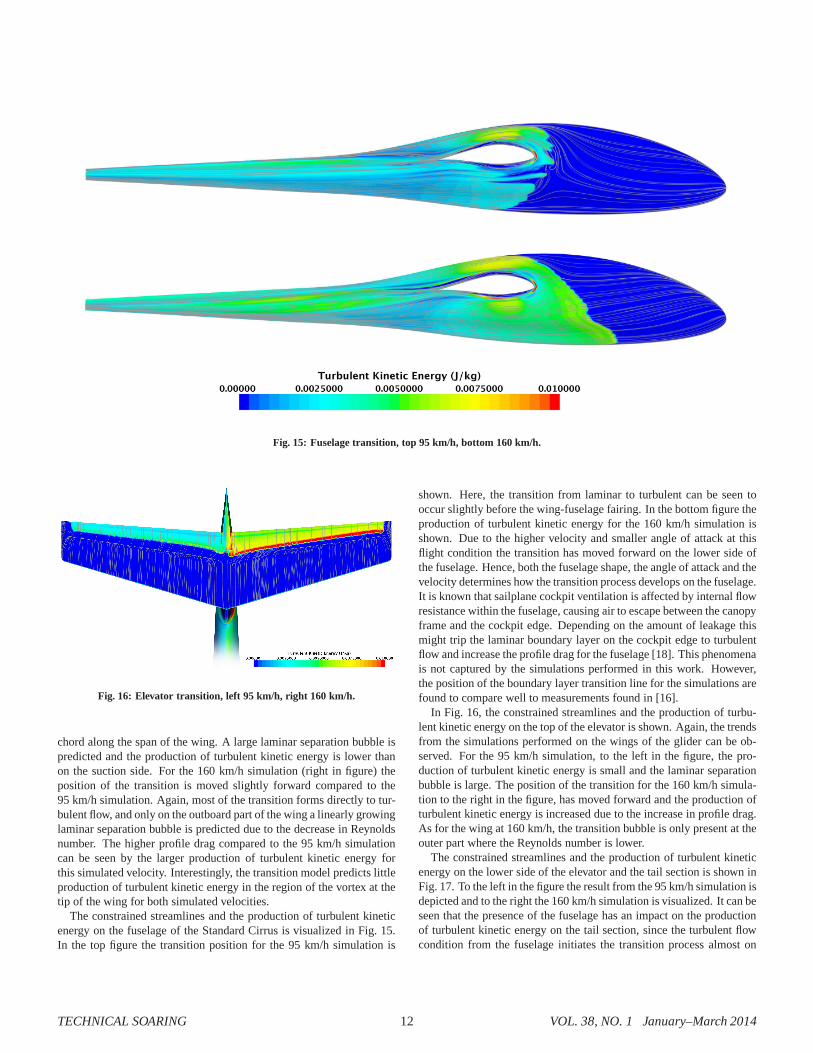
Fig. 15: Fuselage transition, top 95 km/h, bottom 160 km/h.

Fig. 16: Elevator transition, left 95 km/h, right 160 km/h.

chord along the span of the wing. A large laminar separation bubble ispredicted and the production of turbulent kinetic energy islower thanon the suction side. For the 160 km/h simulation (right in figure) theposition of the transition is moved slightly forward compared to the95 km/h simulation. Again, most of the transition forms directly to tur-bulent flow, and only on the outboard part of the wing a linearly growinglaminar separation bubble is predicted due to the decrease in Reynoldsnumber. The higher profile drag compared to the 95 km/h simulationcan be seen by the larger production of turbulent kinetic energy forthis simulated velocity. Interestingly, the transition model predicts littleproduction of turbulent kinetic energy in the region of the vortex at thetip of the wing for both simulated velocities.

The constrained streamlines and the production of turbulent kineticenergy on the fuselage of the Standard Cirrus is visualized in Fig. 15.In the top figure the transition position for the 95 km/h simulation is

shown. Here, the transition from laminar to turbulent can beseen tooccur slightly before the wing-fuselage fairing. In the bottom figure theproduction of turbulent kinetic energy for the 160 km/h simulation isshown. Due to the higher velocity and smaller angle of attackat thisflight condition the transition has moved forward on the lower side ofthe fuselage. Hence, both the fuselage shape, the angle of attack and thevelocity determines how the transition process develops onthe fuselage.It is known that sailplane cockpit ventilation is affected by internal flowresistance within the fuselage, causing air to escape between the canopyframe and the cockpit edge. Depending on the amount of leakage thismight trip the laminar boundary layer on the cockpit edge to turbulentflow and increase the profile drag for the fuselage [18]. This phenomenais not captured by the simulations performed in this work. However,the position of the boundary layer transition line for the simulations arefound to compare well to measurements found in [16].

In Fig. 16, the constrained streamlines and the production of turbu-lent kinetic energy on the top of the elevator is shown. Again, the trendsfrom the simulations performed on the wings of the glider canbe ob-served. For the 95 km/h simulation, to the left in the figure, the pro-duction of turbulent kinetic energy is small and the laminarseparationbubble is large. The position of the transition for the 160 km/h simula-tion to the right in the figure, has moved forward and the production ofturbulent kinetic energy is increased due to the increase inprofile drag.As for the wing at 160 km/h, the transition bubble is only present at theouter part where the Reynolds number is lower.

The constrained streamlines and the production of turbulent kineticenergy on the lower side of the elevator and the tail section is shown inFig. 17. To the left in the figure the result from the 95 km/h simulation isdepicted and to the right the 160 km/h simulation is visualized. It can beseen that the presence of the fuselage has an impact on the productionof turbulent kinetic energy on the tail section, since the turbulent flowcondition from the fuselage initiates the transition process almost on


Fig. 17: Tail section transition, left 95 km/h, right 160 km/h.

the leading edge for the lower part of the fin. Higher up on the fin theinflow condition is less turbulent and the transition occurslater. Also,in the connection between the elevator and fin more turbulentkineticenergy is produced due to increased interference drag, and the transitionpoint is moved slightly forward. For the 95 km/h simulation alaminarseparation bubble can be seen to form about half way up the fin andcontinues on the lower side of the elevator. For the 160 km/h simulation,however, the laminar separation bubble is only visible on the lower sideof the elevator and the transition forms directly to turbulent flow onthe fin section. The drag coefficient for the tail section is found to beReynolds number dependent and a reduction inCd of about 10% isfound for the 160 km/h simulation compared to the 95 km/h simulation.

To obtain converged solutions for the simulations using theγ–Reθmodel the calculated grids are adjusted to fulfil the mesh criteria due todifferences in simulated velocities and angles of attack. Since they✰

value for the mesh scales with the velocity, the grids at highvelocitiesare adjusted using a smaller distance to the first cell centroid. At anglesof attack where the flow is less attached, more cells on the wing arealso needed to obtain a converged solution. The number of cells in themesh for the 90 km/h to the 160 km/h simulation is therefore graduallyincreased from 28 million to about 42 million cells, respectively. Thesimulations of the fuselage and tail section mesh have about7.8 millioncells.

In Fig.18, the calculated speed polar for the Standard Cirrus is com-pared to flight measurements from Idaflieg. The simulations performedusing theγ–Reθ transition model can be seen to compare well to the realflight data. For velocities below 100 km/h the simulations are closelymatched to the in-flight measurements. At higher velocities, the sinkrates are slightly under-predicted. The measured best glide ratio for

60 80 100 120 140 160 180−3

−2.5

−2

−1.5

−1

−0.5

V [km/h]

h [m

/s]

Idaflieg, 2011CFD transitionCFD turbulent

Fig. 18: Standard Cirrus speed polar comparison.

the Standard Cirrus from the Idaflieg flight tests is found to be 36.51 at94.47 km/h. The best glide ratio for the simulations performed usingthe γ–Reθ model is found to be 38.51 at 95 km/h. The turbulent cal-culations of the Standard Cirrus can be seen to heavily over-estimatethe drag and consequently the sink rates for all investigated velocities.The difference between the simulated results and the flight measure-ments also increase at higher flight speeds. This is because the frictiondrag on the glider is increasingly over-predicted since no laminar flowis present in the model. The best glide ratio for the fully turbulent sim-ulations is found to be 28.96 at 90 km/h.

In Table 1 the angles of attack for the Standard Cirrus simulationsare given. The zero angle of attack position for the CFD models ofthe glider is referenced to the weighing position as found inthe flightand service manual [19]. As can be seen in the table, higher angles ofattack are required to sustain steady level flight when performing thesimulations as fully turbulent compared to using theγ–Reθ transitionmodel.

ConclusionsIn this study the performance of the Standard Cirrus glider is simu-

lated using the computational fluid dynamics code STAR-CCM+. Theturbulent flow is modelled using thek–ω SST turbulence model and thetransition locations are automatically predicted using the γ–Reθ transi-tion model. To investigate the performance of theγ–Reθ model, calcu-lations on a Cirrus airfoil are first performed using a two dimensionalgrid. The final three dimensional simulations of the glider are validatedby comparing the results to recent flight measurements from Idaflieg. Itis found that the numerical model is able to predict the performance of

Table 1: Input data for CFD simulations.

V∞ ❬km❂h❪ 90 95 100 110 120 140 160

CL [-] 0.911 0.818 0.738 0.610 0.512 0.376 0.288

αtransition [deg] 2.663 1.770 1.013 -0.207 -1.128 -2.396 -3.220

αturbulent [deg] 3.265 2.274 1.472 0.169 -0.805 -2.133 -2.992


the glider well. For low angles of attack, theγ–Reθ transition model im-proves the results for the lift and drag prediction of the glider comparedto fully turbulent calculations. For high angles of attack theγ–Reθ tran-sition model is unable to converge. The best glide ratio for the StandardCirrus from the flight tests is measured to be 36.51 at 94.47 km/h. Forthe simulation using theγ–Reθ transition model the best glide ratio iscalculated to be 38.51 at 95 km/h. For the fully turbulent simulationsthe best glide ratio is predicted to be 28.96 at 90 km/h. The large devi-ations in the prediction of the performance when using fullyturbulentsimulations are due to the absence of laminar flow in the boundary layerof the glider.

By accounting for the drag due to air leakage from the cockpitedges,as well as the drag from the tail-skid and wing tip skids, the resultsfrom the simulations using theγ–Reθ transition model could be furtherimproved. In particular, the drag of the tail in this work is simulatedusing a simplified model where the elevator is positioned at zero angleof attack. By accounting for the extra induced drag due to theelevatordeflection needed to sustain steady level flight, the resultsshould beimproved. Future studies should investigate the drag production fromthe glider in more detail and focus on applying theγ–Reθ transitionmodel for high angles of attack.

AcknowledgmentsThe author wishes to thank Dipl.-Ing. Falk Patzold at the Technische

Universitat Braunschweig for providing the experimentaldata from theStandard Cirrus flight tests. Also, thanks to Ing. Bernt H. Hembre andGraeme Naismith for their help with measuring the glider geometry andto Dr. Gloria Stenfelt for her support throughout this study.

References[1] CD-Adapco,Introducing STAR-CCM+, 2014, User guide, STAR-

CCM+ version 9.02.

[2] Langtry, R. B. and Menter, F. R., “Correlation-based transitionmodeling for unstructured parallelized computational fluid dy-namics codes,”AIAA Journal, Vol. 47, No. 12, 2009, pp. 2894–2906.

[3] Malan, P., Suluksna, K., and Juntasaro, E., “Calibrating theγ–Reθtransition model for commercial CFD,”47th AIAA Aerospace Sci-ences Meeting including The New Horizons Forum and AerospaceExposition, January 2009.

[4] Robert McNeel and Associates,Rhinoceros NURBS modeling forWindows, 1993–2008, User’s Guide, Version 4.0.

[5] “XFLR5. Analysis of foils and wings operating at low Reynoldsnumbers.” February 2014, Guidelines for XFLR5 v6.03.

[6] Melber-Wilkending, S., Schrauf, G., and Rakowitz, M., “Aero-dynamic analysis of flows with low Mach- and Reynolds-number

under consideration and forecast of transition on the example ofa glider,” 14th AG STAB/DGLR Symposium, Bremen, November2004.

[7] Menter, F. R., “Two-equation eddy-viscosity turbulence modelsfor engineering applications.”AIAA Journal, Vol. 32, No. 8, 1994,pp. 1598–1605.

[8] Somers, D. M., “Experimental and theoretical low-speedaerody-namic characteristics of a Wortmann airfoil as manufactured ona fiberglass sailplane,” Tech. Rep. TN 0-8324, NASA, February1977.

[9] Hansen, T.,Wind Turbine Simulations using Navier-Stokes CFD,Master’s thesis, Royal Institute of Technology, Aeronautical andVehicle Engineering, July 2010.

[10] Pointwise, Inc.,Pointwise, reliable CFD meshing, 2014, Usermanual, version 9.02.

[11] von Doenhoff, A. E. and Abbot Jr., F. T., “The Langleytwo-dimensional low-turbulence pressure tunnel,” Tech. Rep.TN 1283, NASA, 1947.

[12] Drela, M. and Youngren, H., “XFOIL 6.9 User Primer,” Tech.rep., Massachusetts Institute of Technology, November 2001,http://web.mit.edu/drela/Public/web/xfoil/.

[13] Montgomerie, B. O. G., Brand, A. J., Bosschers, J., and van Rooij,R. P. J. O. M., “Three-dimensional effects in stall,” Tech. Rep.ECN-C-96-079, NREL, TUD, June 1997.

[14] Anderson Jr., J. D.,Aircraft Perfromance and Design, McGraw-Hill, 1999.

[15] Patzold, F., “Preliminary Results of Flight Performance Deter-mination of Cirrus75 D-6607 S/N 633,” Tech. rep., IDAFLIEG,2012, Preliminary results from the 2011 IDAFLIEG summermeeting.

[16] Thomas, F.,Fundamentals of Sailplane Design, College ParkPress, Silver Spring, Maryland USA, 1999.

[17] Althaus, D. and Wortmann, F. X.,Stuttgarter Profilkatalog I, In-stitut fur Aerodynamik und Gasdynamik, Stuttgart, 2011.

[18] Jonker, A. S., Bosman, J. J., Mathews, E. H., and Liebenberg, L.,“Flow over a Glider Canopy,”The Aeronautical Journal, Vol. 118,No. 1204, June 2014, pp. 669–682.

[19] Schempp-Hirth K. G., Kircheim-Teck,Flight and Service Manualfor the Sailplane Standard Cirrus, 1969.


Documents

Modeling the Performance of the Standard Cirrus Glider