Modeling storm-induced sediment transport on the inner

W&M ScholarWorks W&M ScholarWorks

Dissertations, Theses, and Masters Projects Theses, Dissertations, & Master Projects

1996

Modeling storm-induced sediment transport on the inner shelf: Modeling storm-induced sediment transport on the inner shelf:

Effects of bed microstratigraphy Effects of bed microstratigraphy

Baeck Oon Kim College of William and Mary - Virginia Institute of Marine Science

Follow this and additional works at: https://scholarworks.wm.edu/etd

Part of the Geology Commons, and the Oceanography Commons

Recommended Citation Recommended Citation Kim, Baeck Oon, "Modeling storm-induced sediment transport on the inner shelf: Effects of bed microstratigraphy" (1996). Dissertations, Theses, and Masters Projects. Paper 1539616714. https://dx.doi.org/doi:10.25773/v5-gzcd-n430

This Dissertation is brought to you for free and open access by the Theses, Dissertations, & Master Projects at W&M ScholarWorks. It has been accepted for inclusion in Dissertations, Theses, and Masters Projects by an authorized administrator of W&M ScholarWorks. For more information, please contact [email protected].

https://scholarworks.wm.edu/

https://scholarworks.wm.edu/etd

https://scholarworks.wm.edu/etds

https://scholarworks.wm.edu/etd?utm_source=scholarworks.wm.edu%2Fetd%2F1539616714&utm_medium=PDF&utm_campaign=PDFCoverPages

http://network.bepress.com/hgg/discipline/156?utm_source=scholarworks.wm.edu%2Fetd%2F1539616714&utm_medium=PDF&utm_campaign=PDFCoverPages

http://network.bepress.com/hgg/discipline/191?utm_source=scholarworks.wm.edu%2Fetd%2F1539616714&utm_medium=PDF&utm_campaign=PDFCoverPages

https://dx.doi.org/doi:10.25773/v5-gzcd-n430

mailto:[email protected]

INFORMATION TO USERS

This manuscript has been reproduced from the microfilm master. UMI

films the text directly from the original or copy submitted. Thus, some

thesis and dissertation copies are in typewriter face, while others may be

from any type of computer printer.

The quality of this reproduction is dependent upon the quality of the

copy submitted. Broken or indistinct print, colored or poor quality

illustrations and photographs, print bleedthrough, substandard margins,

and improper alignment can adversely affect reproduction.

In the unlikely event that the author did not send UMI a complete

manuscript and there are missing pages, these will be noted. Also, if

unauthorized copyright material had to be removed, a note will indicate

the deletion.

Oversize materials (e.g., maps, drawings, charts) are reproduced by

sectioning the original, beginning at the upper left-hand corner and

continuing from left to right in equal sections with small overlaps. Each

original is also photographed in one exposure and is included in reduced

form at the back of the book.

Photographs included in the original manuscript have been reproduced

xerographically in this copy. Higher quality 6” x 9” black and white

photographic prints are available for any photographs or illustrations

appearing in this copy for an additional charge. Contact UMI directly to

order.

UMIA Bell & Howell Information Company

300 North Zeeb Road, Ann Arbor MI 48106-1346 USA 313/761-4700 800/521-0600

Reproduced with permission of the copyright owner. Further reproduction prohibited without permission.

Reproduced with permission of the copyright owner. Further reproduction prohibited without permission.Reproduced with permission of the copyright owner. Further reproduction prohibited without permission.

MODELING STORM-INDUCED SEDIMENT TRANSPORT

ON THE INNER SHELF: EFFECTS OF BED MICROSTRATIGRAPHY

A Dissertation

Presented to

The Faculty of the School of Marine Science

The College of William and Mary in Virginia

In Partial Fulfillment

Of the Requirements for the Degree of

Doctor of Philosophy

by

Baeck Oon Kim

1996


UMI Number: 9701092

Copyright 1997 by Kun, Baeck OonAll rights reserved.

UMI Microform 9701092 Copyright 1996, by UMI Company. All rights reserved.

This microform edition is protected against unauthorized copying under Title 17, United States Code.

UMI300 North Zeeb Road Ann Arbor, MI 48103


APPROVAL SHEET

Approved, June 1996

This dissertation is submitted in partial fulfilment of

the requirements for the degree of

Doctor of Philosophy

Baeck Oon Kim

L. Donelson Wright, PI Committee Chairman/Advisor

32JT

John D. Boon, m, Ph.D.

Jerome P.-Y. Maa, Ph.D.

Lmda C. Scnafmer

V Ole S. Madsen, Sc.D. Massachusetts Institute of Technology

Cambridge, Massachusetts


TABLE OF CONTENTS

ACKNOWLEDGMENTS.................................................................................................................. v

LIST OF TABLES ................................................................................................................................vi

LIST OF FIGURES ............................................................................................................................vii

LIST OF SYMBOLS ........................................................................................................................ x

ABSTRACT........................................................................................................................................xvii

1. INTRODUCTION....................................................................................................................... 2

2. METHODS AND DATA ANALYSIS ...................................................................................... 6

2-1. Introduction.................................................................................................................. 6

2-2. Field Experiments......................................................................................................... 6

2-3. Background of Field S ite .............................................................................................. 8

2-4. Data Analysis ..................................................................................................................12

2-4-1. W ind............................................................................................................. 122-4-2. W ave............................................................................................................. 152-4-3. Current......................................................................................................... 182-4-4. Suspended Sediment.......................................................................................212-4-5. Grain Size....................................................................................................... 23

2-5. Correction of Measurement Heights............................................................................... 26

3. BOUNDARY LAYER PROCESSES COUPLED WITH BED STRATIGRAPHY............. 33

3-1. Introduction................................................................................................................ 33

3-2. Wave-current Boundary Layer Model.......................................................................... 35

3-3. Bottom Roughness....................................................................................................... 41

iii


3-4. Sediment Transport......................................................................................................... 45

3-4-1. Mean Suspended Sediment Concentration Model........................................ 463-4-2. Bedload Transport......................................................................................... 483-4-3. Critical Shear Stress.......................................................................................50

3-5. Sediment Conservation Equation: One-dimensional Model.......................................... 51

3-6. Mixing Depth and Armoring Process............................................................................. 56

3-6-1. Review of Mixing Depth Concept............................................................... 563-6-2. Availability of Sediment.............................................................................. 60

3-7. Solution Procedures.........................................................................................................65

3-8. Results and Discussion....................................................................................................71

3-9. Limitations of the Model............................................................................................... 100

4. ACROSS-SELF SEDIMENT TRANSPORT: 1DH DEPTH-RESOLVED MODEL................ 102

4-1. Introduction....................................................................................................................102

4-2. Wave Transformation Model........................................................................................ 104

4-2-1. Formulation................................................................................................ 1044-2-2. Determination o f Wave Friction Factor.......................................................108

4-3. Current Model................................................................................................................ 114

4-3-1. Formulation................................................................................................... 1144-3-2. Solution Procedures...................................................................................... 1174-3-3. Test of Current Model.................................................................................. 119

4-4. Sediment Conservation Equation..................................................................................126

4-5. Results and Discussion.................................................................................................. 132

5. CONCLUSIONS........................................................................................................................... 157

APPENDIX A

The Effects of Measurement Height Changes on the Velocity Profiles............................ 160

REFERENCES................................................................................................................................. 169

VITAE................................................................................................................................................. 177

iv


ACKNOWLEDGMENTS

I would like to make a grateful acknowledgment for Dr. L. Donelson Wright who guided this

work and provided support, insight and understanding with great patience. I would like to thank my

committee members, John Boon, Jerome Maa, Linda Schaffner, and Ole Madsen. They provided

valuable comments and helped me to make this thesis more readable. I am also grateful to Dan

Hepworth, Frank Farmer, Todd Nelson, and Bob Gammish for helping with data acquisition. Thanks

to Cynthia Harris and Beth Marshall for their hospitality in helping paperwork. Thanks to Sungchan

Kim and Jingping Xu for many valuable conversations. Special thanks to Tom Chisholm for English

corrections. I am thankful that many people of the Virginia Institute o f Marine Science including my

fellow students helped my education and daily life.

I would like to thank Pat Wiberg of the University of Virginia for providing valuable

discussion. The Field Research Facility of the U.S. Army Corps of Engineer provided wind data.

Permission to use these data is appreciated. This research was supported by the National Science

Foundation, Grant No. OCE-9123513.

I would like to thank my parents and brothers for their love, support, and encouragement.

Finally, I would like to thank my wife, Jihyun, for her constant love and great patience through five

years.

v


LIST OF TABLES

2-1. Summary of instrumentation................................................................................................... 9

2-2. Summary of measurement height............................................................................................ 29

2-3. Initial measurement heights measured above bed...................................................................30

3-1. ft (6 J versus f (1 .................................................................................................................62

4-1. Comparison of the JMGM and GM model predictions with field measurements 124

vi


LIST OF FIGURES

2-1. Map showing study area............................................................................................................ 7

2-2. Three-dimensional representation of bathymetry................................................................. 11

2-3. Grain size distribution and cumulative curve of bottom sediment......................................... 13

2-4. Vertical distribution o f sand composition in a sediment core............................................... 14

2-5. Time series of the FRF wind data............................................................................................ 16

2-6. Time series of wave characteristics....................................................................................... 19

2-7. Time series of current velocity.............................................................................................. 20

2-8. Time series of OBS data ....................................................................................................... 22

2-9. Input of bed stratigraphy....................................................................................................... 25

2-10. Time series of DSA data......................................................................................................... 28

2-11. Time series of bed elevation changes.......................................................................................32

3-1. Schematic representation of vertical one-dimensional model.................................................36

3-2. Flow chart of vertical one-dimensional model..................................................................... 67

3-3. Bed stratigraphy formation in vertical one-dimensional model........................................... 68

3-4. Comparison of predicted concentrations (y0 = 0.001) with measurements, at 20 m ............ 72

3-5. Comparison of predicted concentrations (y0 = 0.001) with measurements, at 12 m ............ 73

3-6. Predicted ripple heights......................................................................................................... 76

3-7. Comparison of predicted u.c and zM with measurements at 20 m depth.................................79

3-8. Comparison of predicted u.c and z^ with measurements at 12 m depth................................ 80

vii


3-9. Predicted concentrations using coupled and decoupled models (Yo = 0 .001)...................... 83

3-10. Predicted concentrations using coupled and decoupled models (y0 = 0.0004).................... 84

3-11. Predicted concentrations using coupled and decoupled models (y0 = 0.0002)........................85

3-12. Predicted concentrations using coupled and decoupled models (y0 = 0.0003)........................86

3-13. Predicted concentration profiles using coupled and decoupled models.................................. 87

3-14. Predicted u-c and z,M using coupled and decoupled models......................................................89

3-15. Predicted erosion depth, total depth and sediment size at 20 m d ep th .................................. 91

3-16. Predicted erosion depth, total depth and sediment size at 12 m depth................................... 92

3-17. Predicted erosion depth using coupled and decoupled models (y0 = 0.001)...........................93

3-18. Predicted erosion depth using coupled and decoupled models (Yo = 0.0003)...................... 94

3-19. Predicted bed stratigraphy at 20 m depth................................................................................. 96

3-20. Predicted grain size distributions of individual layers at 20 m depth......................................97

3-21. Predicted bed stratigraphy at 12 m depth.................................................................................98

3-22. Predicted grain size distributions of individual layers at 12 m depth......................................99

4-1. Flow chart of horizontal, one-dimensional model..................................................................105

4-2. The FRF wave height measured at 8 m and 17 m depths................................................... 110

4-3. Predicted wave height with no energy dissipation..................................................................I l l

4-4. Wave transformation model errors in comparison with wave period and wind speed 112

4-5. Predicted wave height with bottom friction......................................................................... 113

4-6. Predicted u.c and u.,* using GM and JMGM models............................................................ 122

4-7. Predicted z^ using GM and JMGM models...........................................................................123

4-8. Comparison of predicted current velocity using JMGM model with measurements............125

4-9. Bed stratigraphy formation in horizontal one-dimensional model...................................... 130

4-10. Comparison of predicted concentrations (y0 = 0.002) with measurements, at 20 m 133

viii


4-11. Predicted across-shelf current velocity field along the transect.......................................... 135

4-12. Predicted along-shelf current velocity field along the transect.............................................. 136

4-13. Predicted concentration field along the transect.................................................................. 137

4-14. Predicted across-shelf local sediment flux field along the transect.................................... 138

4-15. Predicted along-shelf local sediment flux field along the transect........................................139

4-16. Spatial and temporal distribution of predicted u.b..................................................................141

4-17. Spatial and temporal distribution of predicted u.,^................................................................142

4-18. Correlation between u.^, and Au.^,...................................................................................... 143

4-19. Spatial and temporal distribution of predicted across-shelf sediment flux...........................145

4-20. Spatial and temporal distribution of predicted along-shelf sediment flux.......................... 146

4-21. Time series of predicted across-shelf and along-shelf sediment flux at 20 m depth............147

4-22. Time series of predicted u.b and u-^ at 20 m depth............................................................ 148

4-23. Temporal variation of predicted bed elevations along the transect.................................... 150

4-24. Spatial and temporal distribution of predicted bed elevation changes.................................. 151

4-25. Time series of predicted net bed elevation changes and cumulative elevations................... 152

4-26. Predicted bed stratigraphy along the transect........................................................................ 154

4-27. Spatial and temporal distribution of predicted d^ of 1 cm thick bed....................................155

4-28. Spatial and temporal distribution of predicted erosion depth............................................. 156

1. Departure of logarithmic profile due to displacement heights........................................... 163

2. Relationship between logarithmic profile and displaced profile......................................... 164

Lx


LIST OF SYMBOLS

Ab, A1 Complex coefficient

Ab Semi-excursion amplitude

Bb, Bs Complex coefficient

b Distance between wave rays

C Wave celerity

Ca Wind-drag coefficient

Cb Volumetric sediment concentration in the bed

Cg Group velocity

C, Suspended sediment concentration of the ;th size class

Cr Reference concentration

Cs Mixing depth coefficient

c Local bed wave celerity

D, D, Grain diameter

Da Grain diameter related to the total depth

d50 Median grain diameter

d,, Near-bed wave orbital diameter

E Wave energy

f Frequency or Coriolis parameter

Fraction of the /th size class


£ (AZJ Fraction of the /th size class in net bed elevation change

£ (5k) Fraction of the /th size class in the th layer

f; (6 J Fraction of the /th size class in the mixing depth

f, (tit) Fraction of the /th size class in the total depth

f^, Wave friction factor

f w Skin friction factor

g Gravitational acceleration

H Wave height

h Water depth

K Number of bed layers involved in the total depth

Kf Damping coefficient

K, Shoaling coefficient

K,. Refraction coefficient

k Wave number

kb Total bottom roughness

k,,,,, Movable bed roughness due to sediment transport

1^ Ripple roughness

kg Grain roughness

L Wavelength

/ Wave-boundaiy-Iayer length scale (= k u . ^ / co)

N Total number of sediment size classes

 Reynolds average o f pressure

Qx Across-shelf sediment flux

xi


Qy Along-shelf sediment flux

<b Mean bedload transport rate

Re Reynolds number

R^d Grain Reynolds number

S Normalized excess skin friction shear stress

Sw(f) Spectrum of wave orbital velocity

s Relative sediment density

T Wave period

t Time

u a Wind speed

U Mean depth-averaged velocity in across-shelf direction

Ubl Depth-averaged, mean wave velocity

u Velocity in x direction

 Reynolds average of horizontal fluid velocity

u' Turbulent velocity

Ub Near-bottom wave orbital velocity amplitude

U= Current velocity

U-b Shear velocity on bottom boundary

U-c Current shear velocity

U-cr Critical shear velocity

U-cw Wave-current shear velocity

u*» Shear velocity on surface boundary

U*wm Maximum wave shear velocity

^ ’win Maximum skin friction shear velocity


Wave velocity

u^, Maximum wave velocity

il. Free stream velocity

Vt Volume of sediment in transport

Va Volume of sediment available for transport

Vb Volume of sediment in bedload

V, Volume of sediment in suspended load

v Velocity in y direction

w' Turbulent velocity in z direction

wf Fall velocity

x Horizontal axis, East-West direction

y Horizontal axis, North-South direction

z Vertical axis

zb; Bed elevation contributed by sediment of the /th size class

z„ Roughness length (= k,,/ 30)

zM Apparent bottom roughness

Zf Reference height

a Empirical constant

P Constant

Ta Fractional availability index

y0 Resuspension coefficient

At Increment of time step

Ax Increment of spatial step

xiii


Net bed elevation change

Sk Bed thickness of the Ath layer

6 b Background mixing depth

6m Mixing depth

6W Wave-current boundary layer thickness

6 d Energy dissipation rate

C Sea surface elevation

Co Nondimensional roughness length (= z J t)

T1 Bed elevation

Tie Erosion depth

T|r Ripple height

0 Incident angle of wave ray

K von Karraan constant

K Ripple spacing

V Kinematic viscosity

V, Eddy diffusivity

Vt Eddy viscosity

p Water density

Pa Air density

P, Sediment density

° w Standard deviation of wave orbital velocity

Tb Bottom shear stress

‘C'b Instantaneous skin friction shear stress

Tc Current shear stress


* « r Critical shear stress

* c w Wave-current shear stress

Wind stress

Wind stress, x component

Wind stress, y component

^ » m Maximum wave shear stress

x'* v m Maximum skin friction shear stress

Tx Turbulent Reynolds’ stress, x component

Turbulent Reynolds’ stress, y component

4 > .Wind direction

= Current direction

4 > c w Acute angle between wave and current

4 > u , Upper limit of the /th size class in the <{> unit

Lower limit of the /th size class in the <f) unit

Critical Shields parameter

f n , Maximum skin friction Shields parameter

( 0 Radian frequency

Subscripts and superscripts

16 o f 16 th percentile of bed grain size distribution

50 of 50th percentile of bed grain size distribution

84 o f 84th percentile of bed grain size distribution

ano Anorbital

orb Orbital

xv


sub Suborbital

i Grain size class

j spatial step

n time step

X x component of the coordinate system

y y component of the coordinate system


ABSTRACT

Sediment transport during a storm event on the inner continental shelf was detailed through the development o f models based on field experiments conducted at Duck, North Carolina in October 1994. A vertical one-dimensional model (1DV model) was developed by coupling the Grant and Madsen (1986) model with bed stratigraphy to consider real seabeds. Sediment was divided into seven size classes and fractional transport was estimated. Mixing depth and total depth from a simplified sediment conservation equation provided the basis for changing bottom sediment, sediment availability for transport, and armoring processes. These processes involve a feedback between hydrodynamics and bed stratigraphy. A horizontal one-dimensional, depth-resolved model (1DH model) was developed to predict inner-shelf morphological changes. Flow and shear stress fields were calculated using a simple wave transformation model combined with the Jenter and Madsen (1989) model. Sediment flux was computed in relation to fractional transport and armoring processes. The sediment conservation equation was numerically solved to yield bed elevation changes associated with individual size classes. Predictions o f suspended sediment concentrations from both models were adjusted by the resuspension coefficient Yo, resulting in y0= 0.001 for the 1DV model and y0 = 0.002 for the 1DH model, respectively.

The coupling in the 1DV model was critical to predicting suspended sediment concentrations. Hydrodynamic variables, however, were not significantly affected by changing bottom sediment Predicted suspended sediment concentrations were higher during the waning phase of the storm than during the erosional phase. Modeled bed stratigraphy showed fining upward sequences. Wind-driven processes on the inner shelf were interpreted using the 1DH model. The magnitude and the direction of horizontal sediment flux were explained in terms of wind-driven currents. Waves produced a sigmoidal-shaped vertical concentration distribution, explaining horizontal gradients of suspended sediment concentrations. The steepness of the sediment flux gradient due to the waves was correlated with wave height. Synchronization of currents and waves was necessary for large flux divergence and morphological changes. During downwelling currents, deposition occurred on the shoreface whereas upwelling currents were accompanied by shoreface/inner shelf erosion. The inner shelf thus responded as either the sink of sediment or the source of sediment.

Baeck Oon Kim Department of Physical Sciences

Virginia Institute of Marine Science Thesis supervisor : L. D. Wright, Ph.D.

Title : Professor, Virginia Institute of Marine Science

xvii


MODELING STORM-INDUCED SEDIMENT TRANSPORT

ON THE INNER SHELF : EFFECTS OF BED MICROSTRATIGRAPHY


1. INTRODUCTION

The inner continental shelf exists in a morphological continuum from the beach-surf zone

complex to the deeper mid to outer continental shelf (in general 20 to 30 m depth). It can be defined,

from a dynamical point of view, as the region in which nonbreaking waves normally agitate the bed

(Wright, 1995). Breaking and dissipation of shoaling waves drives most surf zone processes.

Seaward of the surf zone, however, various forcing factors such as waves, winds, tides and their

nonlinear interactions govern the complicated inner-shelf dynamics (Nittrouer and Wright, 1994;

Wright, 1995). On the inner shelf, wind stress directly affects water flow and generates advective

currents that affect the bed (Mitchum and Clark, 1986). The inner shelf boundary layer is

characterized by wave-current interactions and involves overlapping surface and bottom boundary

layers. Thus, it is important to understand boundary layer processes in the study of sediment

transport on the inner shelf. For this reason, wave-current interaction models describing

comprehensive boundary layer processes such as the Grant and Madsen (1986) model become

important components of more complex sediment transport models.

Application of benthic boundary layer process models to natural environments demands

considerations of differences between simplified assumptions of theoretical and empirical models and

complicated realities existing in nature. Some important factors include flow acceleration, wave

irregularities, nonhomogeneous sediment and biological effects (Dyer, 1984; Wright, 1989).

However, quantifying each factor is still very difficult because of the lack of field experiments.

Nielsen (1993) showed that formulae for wave-generated ripple geometry obtained from laboratory

2


experiments required modification in order to give agreement with data obtained from measuring

natural bedforms under irregular waves. It has been noted that simple models result in unrealistic

predictions for the direction o f sediment transport and values of roughness parameters because of

micro-scale bedforms (Wright et al., 1991; Wright, 1993). In relation to this, Wright (1993)

emphasized the consideration o f natural sediment to account for the time-related composition of

bottom sediment (bed microstratigraphy).

A primary goal of the present study is to relate time-varying hydraulic roughness to bed

stratigraphy. Bottom sediment in natural environments shows poor sorting and vertical stratification.

Therefore, representative parameters for size distribution of nonhomogeneous sediment, that is,

median grain size and sorting, cannot be constant as is the case for results from controlled laboratory

experiments. By realizing that the size distribution of bottom sediment changes with time-varying

flows through enhanced suspension of sediment, it can be assumed that the size parameter

representing both bottom and suspended sediment is a function of both time-varying shear stress and

elapsed time since the onset of an event Since the geometry of bedforms is governed by the size of

bed material (Middleton and Southard, 1984), hydraulic roughness, which is likely to be influenced

by sediment size and bedforms, is also a function of time.

Since boundary layer processes are mutually dependent on bottom sediment, we need to

consider interactions between flow and the bed. When the mixed and stratified sediment is

incorporated into a sediment transport model, there exists a complicated feedback that involves

changing bottom sediment and armoring processes (Holly and Karim, 1986). Sediment transport

models developed for river channel beds, composed of sand and gravel mixtures, have evolved to

account for the armoring processes (Borah, et al., 1982; Park and Jain, 1987; van Niekerk et al.,

1992). The armoring processes play important roles in controlling sediment transport because these

processes influence flows as well as availability of sediment for transport. Several studies on the


inner shelf included armoring processes (Kachel and Smith, 1986; Wiberg et al., 1994) but lack of

field measurements constrained fully developed models. In this study, a model accounting for

interactions between the flow and the bed is developed to deal with real seabeds. For this purpose, an

approach to simplify the sediment conservation equation is employed to calculate changing bottom

sediment. Also, this provides insights as to the coupling between boundary layer processes and bed

stratigraphy.

Process-based models predicting beach profile changes and coastal morphology have been

used to understand coastal morphodynamic systems (Roelvink and Broker, 1993; De Vriend et al.,

1993). Although various mathematical models were developed by combining different constituent

models of waves, currents, and sediment transport, the models were similar in that the constituent

models were closely coupled to each other based on morphodynamic principles. These principles

state, in brief, that boundary layer processes are the link between hydrodynamics and morphology in

terms of the friction forces. The exerted forces trigger sediment transport and erosion or accretion of

the morphology result from sediment flux gradients. Again, the boundary layer processes depend on

the changed morphology (Wright, 1995). In this study, a process-based model associated with wind-

driven processes is developed to understand the relationship between forcing and response of the

inner-shelf bed. The continental shelf of the Middle Atlantic Bight is classified as storm dominated

(Swift et al., 1985). It is during high energy events that the most significant sediment transport

occurs. Gradients in transport (divergence of sediment flux) cause morphological changes. Across-

shelf sediment transport on the inner shelf exerts important influences on morphological changes

(Swift et al, 1985; Wright et al., 1991; Wright, 1995). Therefore, a model accounting for across-shelf

transport during high energy events has great potential to describe inner-shelf morphodynamic

processes.

One objective of this study is to understand interactions between flows and mixed, stratified


bottom sediment in order to improve our understandings o f boundary layer processes on the inner

continental shelf. Another objective is to integrate these boundary layer processes with a process-

based model to understand relationships between sediment transport triggered by wind-driven

processes and morphological changes of the inner shelf. These objectives are achieved through the

development of two models: a boundary layer process model and a sediment transport model.

Chapter 2 provides description and analysis of data used in the models. In Chapter 3, a vertical one

dimensional model is developed to link boundary layer processes to bed stratigraphy based on a

simplified sediment conservation equation and armoring processes. Using this model, the effects of

bed stratigraphy on hydrodynamics and sediment transport will be examined. However, there are no

laboratory and field measurements to prove these interactions. In Chapter 4, a horizontal one

dimensional, depth-resolved model is developed assuming a simplified geometry for the inner shelf.

This model gives insights as to the roles of storm-driven waves and currents in causing sediment flux

divergence. Also, the effects of sediment transport during a storm event on morphological changes of

the inner shelf is examined using this model. In Chapter 5, the results of these two models are

summarized and conclusions of this study are presented.


2. METHODS AND DATA ANALYSIS

2-1. Introduction

The development of models (presented in Chapter 3 and 4) is based on field experiments.

Field data are used as inputs to the models. The model inputs are the measured quantities such as

winds, waves, currents and bottom sediment. In addition, measured suspended sediment

concentrations, shear velocity, and roughness are used to compare with the model predictions. Since

this study relates the models to storm events, the field experiments require to catch those events.

Therefore, the portion of field data from high-energy events is most useful for the models.

This chapter describes equipments for field experiment, the field site, the methodology for

data analyses, and the results o f data analyses. Winds, waves, currents and bottom sediment data

corresponding to a storm event are selected for the model inputs. Because instrumented tetrapod

experienced vertical displacement during the deployment, a methodology to correct measurement

heights due to instrument displacements is also introduced.

2-2. Field Experiments

As a part of the multi-disciplinary CoOP’94 experiments (Coastal Ocean Processes), the

Virginia Institute of Marine Science deployed two instrumented tetrapods on the inner shelf off the

U.S. Army Corps of Engineers’ Field Research Facility (FRF) at Duck, North Carolina (Fig. 2-1) to

measure the benthic boundary layer flows and resultant sediment resuspension. The two tetrapods

were deployed at depths of 12 m and 20 m on the same transect. Four data sets were retrieved from

6


7

41 N

39 N

m,inUi

37 N

DUCK/

35 NHATTERAS

33 N

31 N1— 80 W 70 W74 W 72 W76 W78 W

Figure 2-1. Map showing study area.


the two missions held in August and October 1994. The October data sets were used in this study

due to stronger and prolonged storm activities.

The instrumentation on each tetrapod during the October experiment is summarized in

Table 2-1. The instruments used in this study were similar to those installed on the tripod described

in Wright et al. (1991). They consisted of a vertical array of four Marsh-McBimey electromagnetic

current meters (EMCM), a Seadata Model 635 directional wave gage incorporating a pressure

transducer and a current meter, a digital sonar altimeter (DSA) and a vertical array of five Downing

optical backscatterance sensors (OBS). Tetrapods were deployed from the R/V Cape Hatteras on 4

October 1994. The measurements were recorded every four hours in bursts consisting of 1024

samples. The sampling rate was 1 Hz.

The individual current meters were calibrated before the deployments with steady flows in a

recirculating flume. The OBS sensors were calibrated after the deployments using a calibration

cylinder (Kim, 1991) with suspended sediment collected in a sediment trap mounted on the tetrapod.

2-3. Background of field site

The study area has several physical characteristics: sand grain size typical of US east coasts,

wave climate and storm exposure representative of US east coasts, regular bottom topography in the

inner shelf, a microtidal range, and a straight coastline (Birkemeier et al., 1985). The dominant wind

direction during the summer season is from the southwest. The wind direction during the autumn and

winter, however, is frequently from the northeast as a result of the extra-tropical storms

(northeasters); westerlies often prevail during intervening periods of high pressure. The high wave

activities occur during October through March and waves come predominantly from the northerly

quadrants. The wave height, for example, reached 3.5 m during an October 1980 storm (Birkemeier

et al., 1985).


9

Table 2-1. Summary o f instrumentation for the October experiment.

Description Inshore tetrapod Offshore tetrapod

Location36 11.994 N 75 42.304 W

36 11.960 N 75 42.480 W

Depth 1 2 m 2 0 m

Period October 4 - November 1 October 4 - November 1

Initial time 1600 EST 1600 EST

InstrumentEM CMPress. TransducerDSAOBS

No. o f burst 137 169 129 169

No. o f burst 168 168 129 173

No. o f samples in one burst 1024 1024

Sampling rate 1 Hz 1 Hz

Burst time interval 4 hour 4 hour


Using the bathymetry data from several sources (Data Announcement 88-MGG-02; Data

Announcement 95-MGG-02), a 3-D representation of bathymetry was constructed (Fig. 2-2). It

shows that the inner shelf (approximately 10 to 2 0 m depth range) is relatively narrow, i.e., the

across-shelf dimension is less than 1 0 km compared with the along-shetf dimension which is order of

100 km. Its shore-normal gradient is steep compared with the mid-shelf where water depth is deeper

than 20 m. The shore-parallel variation of the inner shelf is not significant, while the deeper area

shows irregular topography. For this reason many studies of the inner shelf assume the simplified

geometry in which the alongshore variation of the morphological features is negligible.

Bathymetric profiles and seismograms collected in this area show the concave upward inner

shelf profile (Tiedeman, 1995). The side-scan sonograms indicated the existence of orbital ripples

and a change in sediment type near the 2 0 m contour. Micromorphodynamic study of the sea bed in

this area has shown variation o f bed characteristics depending on the hydrodynamic conditions

(Wright, 1993). During the summer fairweather period, sea beds are composed of large ripples and

biogenic roughnesses. The range of the ripple length and the ripple height was found to be 8 to 15 cm

and 2 to 4 cm, respectively. In both post-storm and winter swell-dominated conditions, small ripples

were observed. The irregular micromorphology was replaced with the highly mobile plane bed during

storm periods.

The grain size analysis of the surface sediment along the shore-normal transect shows a

fining seaward trend, encountering a zone of sandy silt between the 13 m isobath and the 15 m

isobath (Birkemeier et al., 1985). The median grain size along the transect ranges from 0.028 to

0.012 cm. The medium to fine sand at the 12 m contour consists of an approximately 1.5mthick

sand sheet (Birkemeier et al., 1985). A core collected at 20 m depth was composed o f more than

80% sand from the surface to 20 cm depth and had a fining downward trend (Tiedeman, 1995). A

core collected at 9 m depth was composed of more than 90% sand in all depths and had a nearly


11

Figure 2-2. Three-dimensional representation of bathymetry shows that the inner shelf of study area is very narrow and steep.


uniform grain size.

Figure 2-3 shows the grain size distribution and the cumulative curve of the sediment

collected at the surface of 13 m depth during 1992 field experiments. The bottom sediment and

suspended sediment of a sediment trap collected during 1994 field experiment were not confidently

analyzed due to unknown systematic errors. Although there is slight variation of sediment

composition along the transect, the bottom sediment composition shown in Figure 2-3 was used as

input for the models described in Chapter 3 and 4. It is also assumed that the horizontal variation of

bottom sediment composition is insignificant This surface sediment consists of 84% sand fraction,

11% silt fraction and 5% clay fraction with a median diameter d50= 0.0113 cm. The variation of sand

composition from the surface to 15 cm depth is presented in Figure 2-4. The sand composition from

1 cm to 2 cm depth shows the highest value, 85%. Below this layer, sand composition decreases to

the minimum at 5 cm depth. It increases to about 80% at 9 cm depth and below this depth it remains

constant with small fluctuations.

2-4. Data Analysis

For the right-handed coordinate system adopted in this study, the East-West component was

taken to be the x axis, the offshore direction being positive. The North-South component was taken

to be the y axis. The direction of currents, waves, and winds was referenced to true North which is

the positive y axis. These directions were measured clockwise from the true North. For the wave and

wind data, the directions are shown where they are going toward. The data were rotated such that the

new coordinate system was aligned to be parallel with the local coast line (-2 0 ° with respect to true

North).

2-4-1. Wind


13

(a)0 .5

0.4

•.§ 0.3 o2«♦—<DN 0.2 CO

0.1

(b)I 1.

Md=0.01132 cm

So=1.77

1 0 0

80

60

40

0

Size class (phi)

Figure 2-3. Grain size distribution (a) and cumulative curve (b) of bottom sediment. The median diameter is 0.0113 cm and geometric sorting is 1.77. Note that silt and clay fraction (> 4(f)) is less than 2 0 %.


Dept

h fro

m the

su

rfac

e (c

m)

14

70 75 80 85Sand composition (%)

Figure 2-4. Sediment core showing vertical distribution of sand composition in I cm intervals.


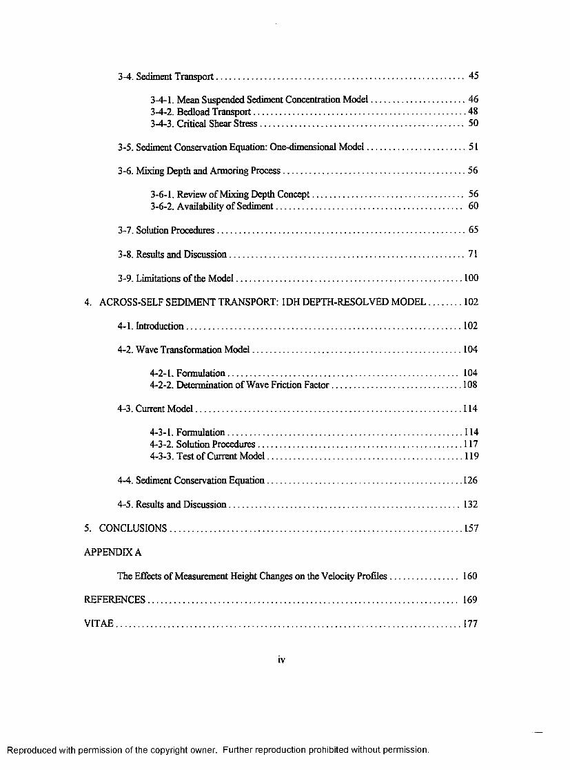
The local wind data used in this study were provided by the FRF. Since they were measured

at 34 minute intervals, it was necessary to select samples corresponding to the sampling interval of

the VIMS data. The magnitude and direction of the local wind in October 1994 showed two events in

which the wind speeds exceed 10 m/s with a highest speed of 18 m/sec (Fig. 2-5). The dominant

direction was from the north during the high wind activities. The two peaks occurred between 10 and

18 in October were separated by a short gap in which the wind speed was reduced to about 5 m/sec

and the direction was from the east

2-4-2. Wave

Following the method described in Chisholm (1993) and Madsen et al. (1993), the wave

characteristics were calculated from the near-bottom velocity measurements. The time series of wave

orbital velocity was obtained by removing current velocity. The rms near-bottom wave orbital

velocity amplitude, ub, is defined by

= & <>w (2-D

where a? is the total variance of the time series of the wave orbital velocity. To estimate wave

direction, u 2 + v 2 and direction were calculated using each u and v pair of wave orbital velocities.

These were converted to a directional distribution with individual 10 directional bins containing the

sum of variances in that direction. A running average using an 11° window smoothed directional

distribution of the wave orbital velocity. It results in two peaks of the directional distribution and

they represent the forward and backward wave orbital velocity differing by 180°. These wave orbital

velocity directions were calculated as the mean of the centroid of each peak. Then the wave direction

was given as the mean o f the two directions.

Each wave orbital velocity was projected to the wave direction. Giving a time series of


16

Wind magnitude and direction

(a)

(b)

ml

10 15 20 25Days from 1 October, 1994

Figure 2-5. Time series of the FRF wind data showing wind direction (a) and magnitude (b) in October 1994. The wind direction is defined as blowing toward.


17

projected wave orbital velocities, a frequency spectrum, Sw(f), was then calculated. From this

spectrum the rms wave period was taken as

7 S J f ld f

f f S J f i d f

where/is the frequency.

Using the values computed from (2-1) and (2-2) and the wave dispersion relationship for

monochromatic waves

co2 = gk tanh kh (2-3)

where to is the radian frequency, k is the wave number and h is the water depth, the significant wave

height Hs can be estimated by

Hs = f t ub T (2 .4 ;

with linear wave theory (Dean and Dalrymple, 1992). To get kh in (2-4), the equation (2-3) needs to

be solved by an iterative method. Alternatively an accurate approximate solution for kh (Hunt, 1979)

can be used, which gives

(kh)2 = y 2 + ------- £-

1 + £ n - 1

where

d v n (2-5)


d, = 0.666..., d2 = 0.355..., d3 = 0.1608465608, d4 = 0.0632098765, ds = 0.0217540484, and d6 =

0.0065407983.

The time series of the wave characteristics observed in October 1994 is presented in Figure

2 - 6 and shows that the maximum near-bottom wave orbital velocities and the maximum wave

periods reached 60 cm/sec and 15 sec, respectively. The only one prominent peak of wave orbital

velocities occurred at the time of the strongest wind (see Figure 2-5) but the trend of wave orbital

velocities was not similar to that of wind speeds. This indicates that the waves were not locally

generated waves. At the onset of the storm, on 10 October, the shortest wave period was recorded

and then it increased monotonously to its maximum value on 20 October when wind speeds had

already died out. This also proves that the wave generation area was further away from the

measurement site, so the swells arrived after local wind ceased. The dominant direction of the waves

was from the southeast except during the period of the onset of the storm when waves arrived from

the northeast. Afterwards wave direction changed, so waves came from the southeast. The

relationships between the local winds and the waves are presented in detail in Kim et al. (in

preparation).

2-4-3. Current

The measured currents of the top current meter (93 cm above bed) at the 20 m site are

presented in Figure 2-7. The largest velocity was about 50 cm/sec occurred at the time of the

strongest local wind, and it was directed predominantly to the south in the along-shelf direction. The

major features of both current speed and directions were closely related to wind speed and directions,


19

VIMS wave at 20 m60

(a)

(b)

h- 10

(C)

225

1801510 20 25 305

Days from 1 October, 1994

Figure 2-6. Time series of wave characteristics showing near-bottom wave orbital velocities (a), wave periods (b), and wave directions (c) at 2 0 m depth.


20

Current magnitude and direction at 20 m

(a)

-10

-20

-30

-40

-50

-60

(b)

E 40

0)20

5 15 20 25 3010Days from 1 October, 1994

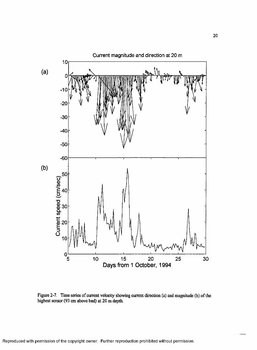
Figure 2-7. Time series of current velocity showing current direction (a) and magnitude (b) of the highest sensor (93 cm above bed) at 20 m depth.


21

indicating a wind-driven current For example, two prominent peaks in the velocity time series from

10 to 17 in October were clearly caused with the peaks in the wind time series. On the other hand, the

minor peak in the late phase of the storm from 17 to 20 in October was not related to the local wind

occurred in that period. The onshore/offshore velocity components appeared to be minimal due to the

much larger along-shetf velocity components. It was argued that the across-shelf velocity

components are small enough to be in the range of the measurement errors, so that this small velocity

can cause an erratic estimation of the sediment flux (Kim et al., in preparation).

2-4-4. Suspended Sediment

Measured values of winds, waves, and currents corresponding to the days from 10 to 20 in

October were selected for the model inputs. This time segment was characterized by a broad peak of

high energy flows which were responsible for most of the resuspension events during the field

experiment. As a result, suspended sediment concentrations increased continuously during the period

from 10 to 16 in October (Fig. 2-8). Both time series of concentrations at 12 m and 20 m depths

appeared to follow those of the wave orbital velocities shown in Figure 2-6. The concentrations at the

1 2 m depth were roughly twice of those at the 2 0 m depth.

The OBS sensors of the tetrapods at both sites showed a steady increase of suspended

sediment concentrations (Fig. 2-8). Thus, the OBS data from all elevations at the 12 m depth and the

lower three elevations at the 2 0 m depth increased beyond the preset maximum concentration of

approximately 5 g/1 during the waning storm phase. Since a maximum concentration is expected to

be measured at the storm peak, the OBS data greater than this value has no physical meaning. This

unrealistic behavior may result from either an electronic drift or a fouling problem. Therefore, the

OBS data were cut off on 16 October. Except this truncation, no data correction was made further.

These truncated OBS data were used for comparisons with predicted suspended sediment


22

(a)20

at 12 m

sensor #

15o>

10

5

0

20at 20 m

sensor #

CD

10

5


Figure 2-8. Time series o f OBS data measured at 12 m (a) and 20 m (b) depths in October 1994. Most OBS sensors give values greater than the preset maximum concentration, 5 g/1, after 16 October.


23

concentrations.

The truncated OBS data indicate some problems in performance of the OBS sensors. As

shown in Figure 2-8 b, the sensor 3 showed greater concentrations than the sensor 2 at the 20 m

depth during the period from 13 to 16 in October. This contradicts a physically reasonable trend in

which we expect a decreasing concentration with elevation above the bed during high energy flows. If

we exclude the sensor 3, the truncated OBS data from the rest of sensors appear to be reasonable

because measured concentrations decrease with elevation. More damage was encountered in the OBS

data at the 12 m depth (Fig. 2-8 a). Measured concentrations from the sensor 1 (not shown in Figure

2-8 a) were greater than the preset maximum capacity of the sensor, 5 g/1, during low energy flows.

The higher three sensors (sensor 3,4, and 5) showed an unrealistic trend of an increasing

concentration with elevation, so these were not acceptable. The quality of the OBS measurements

from the inshore tetrapod was possibly bad.

2-4-5. Grain Size

For the grain size analysis, the general operation for the wet sieving followed Folk’s method

(Folk, 1968). After dividing sediment samples into coarse and fine grain size fractions, the fine grain

size fractions were analyzed by pipette methods to yield the ratio of silt to clay. Then weighted

sand:silt:clay ratio was found to give the preliminary result of the grain size analysis. In order to

estimate grain size parameters using a graphic method (Folk, 1968), grain size distributions from

coarse and fine grain size fractions, each grain size fraction being analyzed separately, were

combined to a grain size distribution. A Rapid Sand Analyzer (automated settling tube) was used for

the sand fraction and a Micrometries SediGraph was used for the silt and clay fraction. Since the fine

grain size fractions in a typical surface sediment from the study area were not enough to be analyzed

using the SediGraph, subsurface samples from a sediment core collected near the 20 m isobath


24

(during 1995 field experiment) were used instead- This substitution for the fine fractions was

acceptable because the ratio of the silt to clay fractions in the subsurface samples was similar to that

of the surface sediment They were combined to form the grain size distribution shown in Figure 2-3

which was used to estimate grain size parameters. The median diameter D in the <j) unit was obtained

by observing the 50 percentile o f the cumulative curve. This median diameter in the <j> unit was

converted to D in the mm unit using the formulation

D [4> unit] = -logj D [mm unit] (2-7)

In the same way, the 84 percentile and the 16 percentile (percent coarser than) were calculated and

converted to and Dl6, respectively. The geometric sorting was found by^Dlf/Du which is about

1.77. This value satisfies the criterion for the armoring processes, in which the sorting value must be

greater than 1.5 (Chinetal., 1994).

A stratified bed generally consists of various layers and each layer can be identified with its

thickness and its grain size composition. When we describe microscale features of bed stratigraphy

(mm to cm scale) as is the case in this study, it is practically difficult to get a unique bed stratigraphy

for certain conditions from field measurements. This makes it difficult to obtain an input of bed

stratigraphy for the model because the surface layers of sea beds are susceptible to continuous

change due to either physical and biological processes. Therefore, it might be reasonable to choose a

simple input, for example, a massive bed (vertically uniform bed showing no structure inside) shown

in Figure 2-9 instead of expending great effort specifying complicated bed stratigraphy. As shown in

Figure 2-9, a simple input can be represented as a matrix form where identical layers with regard to

layer thickness and grain size composition are repeated downward from the surface of a vertical

sediment column. The modeling of the formation o f bed stratigraphy is, however, a different

problem. The proposed model itself can deal with even complicated input of bed stratigraphy,


25

Input of bed stratigraphy

bed size fractionthickness 1 2 3 4 6 8 10

cm (J)

0.0220 0.0151 0.4026 0.4203 0.1058 0.0170 0.01720.0220 0.0151 0.4026 0.4203 0.1058 0.0170 0.01720.0220 0.0151 0.4026 0.4203 0.1058 0.0170 0.01720.0220 0.0151 0.4026 0.4203 0.1058 0.0170 0.01720.0220 0.0151 0.4026 0.4203 0.1058 0.0170 0.01720.0220 0.0151 0.4026 0.4203 0.1058 0.0170 0.01720.0220 0.0151 0.4026 0.4203 0.1058 0.0170 0.01720.0220 0.0151 0.4026 0.4203 0.1058 0.0170 0.01720.0220 0.0151 0.4026 0.4203 0.1058 0.0170 0.01720.0220 0.0151 0.4026 0.4203 0.1058 0.0170 0.0172

Figure 2-9. Input of bed stratigraphy is a matrix consisting of bed thickness and grain size composition of each layer. A massive bed is chosen for simplicity. It is also noted that the number of size classes in silt and clay fraction is reduced to reduce computational time.


26

although this study uses a simple massive bed as input

The size interval of the fine grain size fractions (> 4 <j>) in Figure 2-9 is modified to reduce

the number of the input size fractions as well as the number of iterative processes. This reduces

computational time in a complicated model. Since the fine grain size fractions are not abundant at the

study area, this modification will not cause a significant effect. However, this is not always the case

when a different type of the bottom sediment is encountered.

2-5. Correction of Measurement Heights

The rate of the change of hydrodynamic quantities becomes greater with increasing

proximity to the bed. This boundary effect can cause significant errors in evaluating velocity and

concentration profiles if there are some appreciable discrepancies in measurement heights. Therefore,

it is important to know the variation o f measurement heights with time. A theoretical consideration

for this problem is presented in Appendix A. In the following a method to calculate measurement

heights using DSA measurements will be presented.

The time series of the displacement heights can be obtained using the time series of the

relative distance from DSA to seabed if we know the initial value of this distance. Temporal changes

in this distance can be produced by a combined effect of the sink of the instrumented tetrapod and the

bed elevation changes due to sediment erosion and deposition. At the current stage of our technique,

it is impossible to differentiate between these effects. Since displacement heights are relative distance

changes, the DSA measurements are appropriate for correction o f measurement height changes.

However, an extended use of these data, such as describing the absolute change of bed elevation,

requires careful attention. The reason is that these data involve the combined effects and there is

uncertainty as to the absolute changes of the displacement heights. So the absolute bed elevation

changes are not separable from the DSA measurements.


27

The time series from the DSA of both the inshore and offshore tetrapods are presented in

Figure 2-10. Both showed overall variations of about 25 cm. The DSA ranges varied with time,

forming approximately two maxima and two minima. During the storm period, from 10 to 20

October, the DSA time series from the instrument located at the 12 m contour increased to form a

local maximum and then decreased sharply until it had a second local maximum at the time of

strongest flow condition. After the second local maximum, the time series decreased to a minimum

and then finally increased. The DSA time series from the 20 m depth generally followed the time

series from the 12 m depth but with some time lag and minor differences.

In situ instrument heights above the seabed are routinely observed by divers as the tetrapods

are deployed and retrieved. Unfortunately it was not possible during the October 1994 deployment

due to the high wave activities at the time of deployment. However, measurement heights of

instruments were recorded on the deck of the deployment vessel. In addition to these measurement

heights above the deck, diver observations during the deployment are summarized in Table 2-2. By

using DSA time series presented in Figure 2-10, the initial measurement heights were determined and

are summarized in Table 2-3. In case of the inshore tetrapod, the most reliable record came from a

diver observation. The lowest OBS sensor was 5 cm above bed (hereafter, ab) in early October,

although the exact time of observation was missing. This indicated that the instrument sank

approximately 6 cm (the difference between the lowest OBS height above the deck and the diver

record) early in the deployment. The DSA time series possibly ranges between 118 and 120 cm

during the time of diver observation. The initial displacement height, 6 cm, was added to these

values, getting a range from 124 to 126 cm, which turns out to be close to the initial measurement

height of DSA above the deck, 127 cm. The error 1 to 3 cm, which is within 3% error, is acceptable

considering that the deck surface was not flat. Therefore, the lowest EMCM and OBS sensors were

estimated to be 5 cm ab at the time of the deployment.


28

(a)

12 m1.2

O)

0.9 JL

1.65

1.6

E 1.55

O)20 m

1.45

j.1.350 5 10 15 20 25 30


Figure 2-10. Time series of DSA data measured at 12 m (a) and 20 m (b) depths.


29

Table 2-2. Summary of measurement heights for the October experiment

Instruments Inshore tetrapod 1 2 m

Offshore tetrapod 2 0 m

ab+ ad ° ab adDSA N/A 127 N/A 152

EMCM1 N/A l l x N/A 152 41 443 71 754 105 104

OBS1 N /A l l x N/A 182 42 443 71 754 107 1045 125 131

Diver measurement 5 3(OBS 1, in early October) (EM CM 1, 1 Nov.)

t above the bed (cm) O above the deck (cm)

X buried during deployment o f tetrapod


30

Table 2-3. Initial measurement heights measured above the bed (cm).

Instruments Inshore tetrapod 1 2 m

Offshore tetrapod 2 0 m

EM CM1 5* 42 35 333 65 644 99 93

OBS1 5* 72 36 333 65 644 1 0 1 935 119 1 2 0

X buried during deployment of tetrapod


Diver observations of measurement heights of instruments on the offshore tetrapod were

collected at the end of the experiment. In spite of the truncation of the DSA time series, it was

assumed that the later DSA values (about 140 cm) can be extrapolated to the end of the experiment

and related to the observed 3 cm ab of the lowest EMCM. Using the fact that the initial DSA ranges

were similar to the values at the end, it was proposed that the tetrapod initially sank approximately

11 cm. So the initial value of the DSA time series was related to a position of 4 cm ab for the lowest

EMCM sensor. The smallest value of the DSA time series over the deployment was not much

different from the initial value. This small variation doesn’t allow burial of the lowest EMCM sensor

during the deployment.

Based on the time series of the displacement heights, the time-varying measurement heights

were used for the calculation of shear velocity and roughness parameters. The fact that the inshore

tetrapod experienced much more vertical displacement than the offshore tetrapod and the lowest

sensors of the inshore tetrapod were buried during the early phase of the storm reduces confidence in

the inshore data set.

The time series of the DSA could be converted to a time series of bed elevations (Fig. 2-11

c), if sinking of the instrument after the deployment is not considered. The initial value of the DSA

time series is simply translated to the zero elevation. Time series of two hydrodynamic variables,

wave orbital velocity and current from both inshore and offshore sites, are also presented in Figure 2-

11. The major features of the bed elevation changes in this study are somewhat different from those

described in Wright et al. (1986), where bed elevation changes were closely related to the wave

orbital velocities and so consisted of an erosional phase at the storm peak and a depositional phase

after the event In contrast, the two depositional phases of bed elevation changes were apparently

associated with the waning phases of two peaks in the current velocity time series, interrupted by an

erosional phase during the storm peak coinciding with the strongest wave orbital velocity.


32

100(a)

(b)

(c)

12m

20m-10

-2020 25 305 10 15


Figure 2-11. Time series of near-bottom wave orbital velocities (a) and current velocities (b) at 12 m and 2 0 m depths are compared with the time series of bed elevation changes (c ) at the two locations.


3. BOUNDARY LAYER PROCESSES COUPLED WITH BED STRATIGRAPHY

3-1. Introduction

It has been proposed that time-varying roughness should be considered in the bottom

boundary layer processes when we deal with beds of mixed and stratified bottom sediment. This is

because the roughness varies with the changes in grain-size distribution in the uppermost part of the

sediment column due to sorting during sediment transport (Parker and Klingeman, 1982; Hill et al.,

1988; Kuhnle, 1989; Wilcock and Southard, 1988; 1989; Wilcock and McArdell, 1993). In armored

beds of river channels with unidirectional flows, variations of grain-size distribution with time have

been simulated using various numerical models (Borah et al., 1982; Lee and Odgaard, 1986; Park

and Jain, 1987; van Niekerk et al., 1992). In a sensitivity analysis conducted by Bedford and Lee

(1994), the grain-size distribution parameter was found to be most sensitive using a bottom

boundary layer model which followed the Glenn and Grant model (Glenn and Grant, 1987). In

addition, a range of bottom sediment conditions will occur during the course of erosion/deposition for

a given stratified sediment. Therefore, assumptions of constant sediment parameters which have been

widely used in the sediment transport literature become inadequate from the theoretical point of view.

Since flow conditions and responses o f bottom sediment are mutual (Holly and Karim, 1986;

Wright, 1993), there are significant interactions between the bed and the flow. It is natural to model

these interactions with a bed of mixed and stratified sediment to completely describe the boundary

layer processes. Numerical models dealing with sediment transport for alluvial channels have focused

on the behavior of the mixed or active layer in attempts to quantify changes in the sediment size of

33


34

the armor or surface layer (Borah et al., 1982; Lee and Odgaard, 1986; Park and Jain, 1987; van

Niekerk et al., 1992). These models linked successfully the concept of mixing depth in the bottom

sediment to the controls of sediment transport As Lu and Shen (1986) pointed out, most models

were similar in the respect of the hydrodynamic routine but treated mixing depth and armoring

processes in different ways.

A few researchers have tried to include beds of mixed sediment in the models for continental

shelf bottom boundary layers (Shi et al., 1985; Kachel and Smith, 1986; 1989; Lyne et al., 1990;

Wiberg et al., 1994). The lack o f Geld measurements over the inner shelf with regards to time-

varying roughness parameters has severely limited the development of a fully described model such

as those used for river beds. These simple equilibrium models have neglected the fact that changes in

the grain size composition affect sediment transport and the resulting sediment transport alters

bottom roughness. In this chapter, the feedback relation between flow and sediment is a major

consideration in the development o f a new model in which the procedure of sediment stratigraphy

formation is incorporated with this feedback relation. Although this model is based on a steady state

assumption, it can also be used as a time-dependent model in limited conditions, assuming that

equilibrium state is reached in a time scale of several hours. This time scale is similar to the time

interval of the field measurements in this study. Although there is no way to verify changes in bed

sediment, there are some indirect ways to determine whether the results of model calculations are

reasonable. For example, one possible way comes from monitoring suspended sediment

concentration, which is relatively easier to measure than monitoring bottom sediment, under the

assumption that changes in the bed are directly linked to resuspension activity.

In this chapter, a vertical one-dimensional boundary layer model (1DV model) that is

coupled with bed stratigraphy is developed to examine the effects of mixed and stratified sediment on

hydrodynamics and sediment transport. Figure 3-1 shows all components which are integrated to


35

construct the model. These include a wave-current interaction model, a bed roughness model,

sediment transport equations associated with the sediment conservation equation, and bed

stratigraphy formation. The combined boundary layer model based on the two-layer eddy viscosity

profile by Grant and Madsen (1979; 1986) is used because its simplicity makes it easy to incorporate

this component into the model. Fractional sediment transport of each sediment size class is used to

estimate for both bedload and suspended load. Procedures to calculate the changing bottom sediment

and the sediment availability for suspended sediment transport are proposed by simplifying the

sediment conservation equation. These procedures are associated with an armoring process. A

mutually dependent feedback between hydrodynamics and bed stratigraphy based on these processes

is proposed but it is emphasized that the approach utilized is not unique. Solution procedures are

described, followed by results of the model. Finally the limitations of the model are discussed.

3-2. Wave-current Boundary Layer Model

Grant and Madsen (1979; 1986) and Madsen (1994) developed the wave-current boundary

layer model used in this study. Their model calculates the velocity profiles and the shear velocities for

the combined wave-current boundary layer. The shear velocities are necessary for the calculation of

sediment transport. Neglecting the Coriolis term and surface wind stress, the simplified, linearized,

Reynolds-averaged equation of motion within the bottom boundary layer (Grant and Madsen, 1979;

1986) becomes

d _ 1 d _ d<u 'w ^ dt ' p & " dz ( }

in which t is time, z is the vertical coordinate measured positive upward from the bottom, p is the

water density, u is the horizontal fluid velocity in the x-direction, w is the vertical fluid velocity, p is


36

O 'Ui><_i>-0£.<OzDOGQ50KI-0co

>xa<ac.CDi-<a.h<0ainoa

INITIALBED

SURFACE

a(AUJZ*axK-QUIID

CURRENT BOUNDARY LAYER

WAVE-CURRENT BOUNDARY LAYER

BEDLOAD

MIXED LAYERMIXED LAYER

nt

BED AT EQUILIBRIUM

DRAIN SIZE INITIAL BED

Figure 3-1. Schematic representation showing boundary layer processes coupled with bed stratigraphy. It consists of wave-current interaction model, sediment transport associated with sediment conservation equation, and bed stratigraphy formation.


TOTA

L V

OL

UM

E

IN T

RA

NS

PO

RT

the pressure, the prime denotes the turbulent fluctuation and the angle brackets represent the

Reynolds-averaging process. Using a turbulent eddy viscosity v „ the turbulent flux of momentum

- in equation (3-1) can be related to the vertical gradient o f the mean fluid velocity by

(3-2)

and the eddy viscosity is modeled under the assumption that the eddy viscosity varies linearly with

the distance from the bottom (Grant and Madsen, 1979; 1986). Incorporating the shear velocity

u w , based on the combined bottom shear stress inside the wave boundary layer, and the

shear velocity uk = , based on the current bottom shear stress, the eddy viscosity is given as

a function of the elevation by

where 5 ^ is the wave boundary layer thickness that is defined as 5wc = in which k = 0.4 is

the von Karman’s constant and co is the wave radian frequency (Grant and Madsen, 1979).

With the assumption of the time-invariant eddy viscosity, the pressure and velocity terms

can be resolved into the current and wave components. Dropping the angle brackets for clarity and

following the manipulation shown in Grant and Madsen (1986), we have the equation for the wave

where uw is the wave velocity and «_ is the free stream velocity. And the equation for the current is

given by

v, = r a w f ° r 2 < 5ht

= ku ^z fo r z > b vc(3-3)

d(uw - u j = d 3(uw - u j dt dz ‘ dz

(3-4)


where ue is the current velocity. The approximate wave solution for (3-4) is found in Grant and

Madsen (1986). This assumes a periodic wave motion specified by the near-bottom wave orbital

velocity = «6cos(ci)t) and a no-slip boundary condition at the bottom roughness z0

=ub In(z/z„)

(In C0 - 1.15)2 + I Iin C O S Clit

(3-6)

where ub is the maximum near-bottom wave orbital velocity and Co is the nondimensional roughness

length given byC0 = z j l ~ current solutions for (3-5) are given as follows. With

a no-slip boundary condition at the top of the bottom roughness this equation is valid forz <

u_ = U *c i Z—— In—zo

(3-7)

For z > 8 ^ , the current velocity profile can be written as follows with the apparent bottom roughness

U *c . Zu„ = — In— (3-8)

Since «.w is an unknown, we need a condition for the maximum wave shear stress to

close the problem, that is


39

u . d mdz (3-9)

and the combined shear stress is given as the vector addition of the shear stress due to the

wave and the shear stress tc due to current, which leads to

(3-10)

Inserting (3-6) into (3-9), Grant and Madsen (1986) gave

' r / \ 2

In - 1.15 +[ t ) 1ZfXO \ 0 l ) J

They further express equation (3-10) in terms of as

2 - r 2 U ^ w = S M*wm (3-12)

where

Cjj = (1 + 2 p cos ^ + p2) 1/2 (3-13)

in which <(>„, is the angle between wave and current and p is

*wm/(3-14)


In the case of weak currents with strong waves, which is a typical case on the inner shelf, p « l and

alternately ~ 1. Under this condition, = f w. We may have the following relationship for the

wave friction factor

(3-15)

However, in the case of storms, this relationship may be not well justified because the currents are

more strongly forced. Based on equations (3-11), (3-12), and (3-15), Grant and Madsen (1986) gave

an approximate expression for the wave friction factor related to bottom roughness in the presence of

waves and currents.

When current, periodic wave characteristics, and bottom roughness are given, equations

from (3-4) to (3-16) can be solved for the velocity profile and shear velocities. Depending on the

specification of the current, the method of solution has different procedures (Madsen et al., 1994). In

this section, solutions are sought for the case in which the current is specified at a reference height.

When flows interact with the bottom sediment, if there are wave-generated ripples and sediment

transport, both bedforms and sediment transport increase the total bottom roughness. This enhanced

bottom roughness affects the flows. Since the ripple generation and sediment transport are estimated

by the flow parameters which are solutions of the above equations, there is mutually dependent

relationship between the bottom roughness and flow parameters. Therefore, these equations are

solved iteratively until an equilibrium state is established In the following section, formulations of

the bottom roughness are described

/ \

+ logC it

= log - 1.65 + 0 .2 4 (4 ^ ) (3-16)


41

3-3. Bottom Roughness

The solution for the velocity profile requires knowledge of the bottom roughness, kb which is

given by

k b = kg + k br + k *n (3-17)

The grain roughness kg is equal to the grain diameter D, and the ripple roughness kbr is given by

Nielsen (1981) in terms of the ripple geometry, the ripple height qr and the ripple spacing Ar

k bT = 8 V r

( \

I k (3-18)

By way of comparisons of several models, Xu and Wright (1995) proposed a movable bed roughness

k ^ due to sediment transport as

ktrn = 5 DS (3-19)

In equation (3-19), is the critical Shield parameter and ijj'm is the maximum skin friction Shield

parameter which can be calculated as follows

i|f' = ------- —— (3-20)p(*-l)g£>, 1 '

where s = p jp =2.65 is the relative sediment density. The maximum skin friction shear stress is

related to ub through the skin friction factor j 'wc.

= J P f» c ul (3-21)


42

Predictive models for the ripple geometry in a wave-dominated environment have been

proposed by several studies (Nielsen, 1981; Grant and Madsen, 1982; Wiberg and Harris, 1994).

Wiberg and Harris (1994) developed equations for predicting ripple type and geometry based on

sediment size, near-bed wave orbital diameter d0, and estimated anorbital ripple height. The wave

orbital diameter is defined as the wave-induced water particle excursion near the bed and this is

easily estimated using da = H!smh{kh) , where the wave height H should be based on the significant

wave height. Nielsen (1981) and Grant and Madsen (1982) used wave orbital amplitude (half of the

wave orbital diameter) and a nondimensional skin friction factor through a friction factor. Wiberg

and Harris (1994) compared the proposed models using a large data set of laboratory and field

measurements and argued that their model is simple and accurate. Since Wiberg and Harris’ model

unified laboratory and field measurements, it doesn’t differentiate the case between laboratory and

field as does the Nielsen’s method. Their model also provided much better estimates of ripple

geometry than the Grant and Madsen’s method. For this reason, this study followed the Wiberg and

Harris’ model for ripple geometry.

Wiberg and Harris (1994) described ripple types as follows. There are three categories

depending on the relationship between ripple spacing Ar and wave orbital diameter. When ripple

spacing is proportional to d0, these ripples are defined as orbital ripples. When ripple spacing is

almost independent of d0 and is a constant multiple of sediment size, these ripples are defined as

anorbital ripples. Anorbital ripples occur at large values o f the wave orbital diameter compared to

sediment size. The transitional group between orbital and anorbital ripples falls into suborbital

ripples. In the continental shelf, most ripples are found to be suborbital and anorbital ripples. These

ripple types can be predicted in terms of the ratio o f the wave orbital diameter to the anorbital ripple

height T|arK>. They provided the classification criteria for the predicted ripple types as follows


43

4 A U , < 2 0

<AU, > 100

20 < 4 / iW , < 100

fo r orbital ripples

fo r anorbital ripples

fo r suborbital ripples

(3-22)

Following Wiberg and Harris (1994), ripple geometry is calculated in terms of ripple

spacing and steepness, defined as The ripple height t |r is simply calculated from the product of

ripple spacing and steepness. The ripple spacing of the anorbital ripple is given by

A = 535 D'ano s

and the steepness of the anorbital ripples is expressed as

(3-23)

lr— = expr

/ , >2dn dn

-0.095 In— + 0.442 In— - 2.28I ^ rj

(3-24)

Equation (3-24) is solved for the ripple height by an iterative method using (3-23). Then the

estimated ripple height is used to determine ripple types according to (3-22) and if this procedure

indicates anorbital ripples, the evaluation of the ripple geometry parameters is satisfied. In the case

of orbital or suborbital ripples, the parameters of the ripple geometry should be reevaluated as

follows (Wiberg and Harris, 1994). For the orbital ripples,

K t - 0.62 d„

( V * U - 017

For the suborbital ripples, the ripple spacing is obtained from

(3-25)


44

b W O " 100In 2 0 - In 1 0 0

(3-26)

and the suborbital ripple height is computed by = (rir / Xr) X ^ with (3-24).

It is noted that the Wiberg and Harris’ model for the ripple geometry doesn’t involve any

explicit consideration of the nondimensional Shields parameter . When the flow condition is such

that i|r'm is less than the critical Shields parameter ), there is no motion o f sediment and

consequently no ripples are generated. In some cases, there exist ripples which are inherited from

earlier events but these are not predictable. There is also a critical value of Tjf'm (> 0.8) where ripples

are washed out and this results in a flat bed (Wilson, 1989). Thus, the range of i|r'm, 0.05-0.8, can be

defined as the conditions under which ripples may be active. Wiberg and Harris (1994) defined these

active ripple conditions as the range of dJDs which was roughly 3 x 103 -104 when the wave period

of T= 10 sec was considered. So it is necessary to examine whether the range of d /D s is similar to

that of t|f'm for the active ripple conditions when dJDs is converted to . The orbital diameter

d0 = 2 ubl co can be related to the shear velocity u !mwm = (T/tim/p ) ly2 through the wave friction

factor = 2(u' On hydraulically rough flows (Re = u ,mikbN > 70), most of the cases

in field environments, the wave friction factor depends on a nondimensional parameter AJkh where

A b = dJ2. Since AJkb is unknown, the computation of wave friction factor or shear velocity from an

orbital velocity is not straightforward. Alternately, as a rough estimation, the wave friction factor can

be assumed to be of the order 0.01 for the range of Af/kb, 10-104. For the active ripple conditions of

d/D„ the range of ub becomes approximately 10-30 cm/sec when D, and T are taken as 0.01 cm and

10 sec, respectively. U sing/^ = 0.01 and g (y-1) D, ~ 15 in equation (3-20), the range of i(j'm

corresponding to the range of ub is 0.03-0.3 which is on the order of i|j'm (= 0.05-0.8). This indicates

that the range of dJD is similar to that of i|/'m for the active ripple conditions.


45

3-4. Sediment Transport

The sediment transport equations can be separated into bedload and suspended load. In

coastal areas, a considerable amount of sediment moves in suspension (Wright et al., 1991; Nielsen,

1993). Although bedload contributions are negligible, it is interesting to treat bedload as analogous

to suspended load in an attempt to make both bedload and suspended load have an equivalent

dimension of volume. Thus, these can be easily incorporated in a sediment conservation equation

which is discussed later.

Individual sediment transport equations corresponding to the size classes of the bottom

sediment, which are defined as fractional transport equations, can be expressed for each size class.

Fractional transport equations, for both bedload and suspended load, are appropriate to deal with

mixed sediment. The number of equations depends on the number of the size classes, which are

determined based on the sediment size distribution. The transport equation of each size class behaves

as if it is based on the single grain size representative of the size class. There is no interaction

between each size class.

The representative sediment size of each size class, denoted as D„ can be given as the

geometric mean of the size class. So the size parameter of the /th sediment size class in the mm unit

is expressed as

‘f r a ♦ <fri»

Dj = 2(3-27)

in which <J>, t and <J>Ih, represent the upper and lower limit of the /th size class in the <j> unit. The

fraction of a size class is assigned as and the sum of all / must be unity, that is

E / = 1 (3-28)i-t


46

in which N is the total number of the size classes. In this study sediment are divided into seven size

classes (Fig. 2-9).

3-4-1. Mean Suspended Sediment Concentration Model

The following suspended sediment concentration model which is used for a sediment

transport module is described in Madsen et al. (1994). Suspended sediment concentration profiles are

calculated by a Rouse type equation which uses an eddy viscosity profile from the wave-current

interaction model. In designating the reference concentration, it is necessary to consider the problem

of sediment availability which is discussed later.

The time-averaged suspended sediment concentrations of the individual size classes are

computed from the diffusion equation (Madsen et al., 1994). Assuming steady state, the governing

equations are

d , d' %

sc,'(3-29)

in which C, is the local suspended sediment concentration of the /th size class, wf i is the fall velocity

of the /th size class and v , is the eddy diffusivity. The eddy diffusivity is assumed to be related to the

eddy viscosity by vj = p vt. The value of p may be controlled by vorticity due to bedforms and

particle inertial effects as summarized in Hill et al. (1988). Glenn and Grant (1987) proposed a

correction for sediment-induced stratification of the near-bed flow through an eddy diffusivity

scheme. This correction may be important for coarse sediment, fine to medium sands, during high

energy flows. There is, however, no conclusion for the value of P (Hill et al., 1988). When we assume

a neutral flow, this constant can be taken as unity (Vincent and Green, 1990). We assume further that

eddy diffusivity is identical in all size classes for simplicity. Then, as the similar form of eddy


47

viscosity (3-3), eddy diffusivity becomes

v, = f ° r z 5vc(3-30)

Assuming that wf i is a constant and integrating (3-29) with the condition of zero vertical flax through

upper boundary results in

The boundary condition of (3-31) is taken as the reference concentration of the /th size class,

Cr j, at a certain height above bed. The mean reference concentration is determined following the

Smith and McLean (1977), which reads

where Cb is the volume concentration of the sediment in the bed, Yo is the resuspension coefficient,

and S, is the mean normalized excess skin friction shear stress of the /th size class. It may be

appropriate to take the reference height zr as the bedload layer thickness, so that from (3-17) and (3-

19) we have

Following Madsen et al. (1994), St can be obtained from the instantaneous normalized skin friction,

|t£j / t 1 , where is the instantaneous skin friction shear stress and is the critical shear stress

of the /th size class. For wave-dominated storm conditions, the skin friction shear stress is assumed

(3-32)

(3-33)


48

to be dominated by wave motion in the suspension of bottom sediment For this reason,

|t£| = |cos o>/[. After averaging the instantaneous normalized skin friction over a wave cycle, one

obtains

*‘ - kTC

V N«wn

U V

(3-34)

in which u is the shear velocity based on the maximum skin friction shear stress and u . ^ is the

critical shear velocity of the /th size class.

With two-layer linear eddy diffusivity given by (3-30) and the boundary condition given by

(3-32), Madsen et al. (1994) gave the solution for the elevation-dependent time-averaged

concentration as follows

C = CS r, I\ 2rj

fo r z < 5 (3-35)

and

[ O■ wf.l ( , > -J5&L

= c zr ,i

6 ~fo r z > 5 (3-36)

3-4-2. Bedload Transport

For the bedload sediment transport rates of the individual size classes, Sleath’s (1978)

formula was adopted because it expresses explicitly the grain size parameter. This allows fractional

sediment transport to be easily obtained. The mean transport rate qb l , averaged over half a wave

cycle, can be written by


49

(3-37)

where ij/,^ is the maximum skin friction Shield parameter and iJj^ is the critical Shield parameter for

the /th size class D„ respectively. It is noted that equation (3-37) is not a net transport rate which will

be zero due to wave symmetry. Here, the mean transport rate during half a wave cycle is of

theoretical interest in the following way.

We must convert the dimensions of the bedload transport rate (cm2 /sec) to volume of the

sediment per unit area (cm) in order to add it to suspended sediment concentration which has a unit

of volume per unit area. Then, we can calculate the total amount of eroded sediment. To do this, it is

necessary to define a mean velocity for the bedload material velocity. Dividing a mean transport rate

by this velocity, the bedload volume can be estimated. Some studies (Madsen, 1991; Nielsen, 1993)

showed that mean velocity is on the order of several times the friction velocity based on theoretical

analysis. Shi et al. (1985) suggested that the mean velocity of the bedload material for the combined

wave-current flow is 10 u. ,/71;.

In a different way, the velocity of the bedload material can be estimated using the wave-

current interaction model described in the above. Since a sediment particle responds and reaches its

terminal velocity in an extremely short time compared to the time scale of the mean turbulent flow

(Madsen, 1991), the velocity of the near-bed flow can be used for calculating that of the bedload

material. A depth-averaged, mean wave velocity during half a wave cycle can be obtained as follows

Here, the range of integration of the near-bed flow velocity with respect to elevation starts from the

(3-38)


50

bed surface to the height of bedload layer zr

3-4-3. Critical Shear Stress

There has been debate about critical shear stresses for bedload transport when heterogeneous

sediments are involved (Parker and Klingeman, 1982; Wilcock and Southard, 1988). If mobility of

all sizes is equal, the grain size distribution o f a poorly sorted sediment is not important and

complicated fractional transport can be simplified using a representative value of the grain size

distribution (Parker et al., 1982). But some geological evidences suggest that entrainment is

selective. In this study, the relationship suggested in Wilcock and Southard (1988) is adopted, which

is given by

U - U *cr,/ *ciyn^50 )

(3-39)

where and u . ^ are the critical shear velocity of the /'th size class and the median diameter of the

sediment, respectively, D, is the geometric mean of the /th size class, Dso is the median diameter, and

a is 0.08. The coefficient a was determined from wave flume experiments using sandy sediments in

which size classes range from 0.01 to 1 cm (Tanaka, 1988).

To calculate the critical shear velocity of the median diameter, the formulae presented by van

Niekerk et al. (1992) are used. Approximate expressions of the Shields curve are given by the

following three equations

<lfCT = 0A(ReDy 03 for ReD < 1 (3-40)


W o ) = _ 2 -2 6 ■ ° - 9 0 5 H & J + 0.168 In\R eD) fo r 1 < ReD < 60 (3-41)

Vcr = 0.045 fo r ReD > 60 (3-42)

In these equations, ijr is the critical Shields number and the grain Reynolds number ReD is given by

u ^ . D*nReD = (3-43)

in which u.^ is the critical shear velocity that is unknown and v is the kinematic viscosity. Both

and ReD are functions of the shear velocity and sediment size. Thus equations (3-40) to (3-42) can be

solved for the critical shear velocity if Dso is given.

3-5. Sediment Conservation Equation: One-dimensional Model

The exchange of sediment between suspension in the water, moved as the bedload and stay

as the bed can be solved using the continuity equation of sediment which is a function of time and

space

where Cb is the bed concentration, q is the bed elevation that is positive downward from a reference

level, t is time, Vt is the volume of the sediment in transport per unit area (cm3/cm2), and Qx

represents the sediment flux in the x direction. The added physical processes, i.e., the processes of


52

bed armoring and grain size changes of bottom sediment, make it impossible to get a formal

algebraic equation of (3-44) (Holly and Karim, 1986). However, a simplification o f the sediment

conservation equation is made in this section to get a physical meaning of mixed, stratified sediment

processes. The schematic representation for this purpose is shown in Figure 3-1.

The conservation equation (3-44) says that the change in the bottom elevation with time

equals the change in the volume of sediment in transport with time plus the change of horizontal flux

with space. By neglecting the spatial gradient of horizontal flux and assuming that flows reach an

equilibrium with bed stratigraphy at each time step during the sequence of time-varying flows,

integration of (3-44) over time elapsed from an initial state gives

Cb % = (K + Vb> at time ' (3-45)

where r|e is defined as an erosion depth at time t below the initial bed surface and Vs and Vb are the

volume of sediment at time t due to time-integrated suspended load and bedload, respectively. It is

noted that the calculation of q,. and Vs + Vb at each time step always refers to the initial bed surface

(Fig. 3-1). The initial bed surface is set at the time of no transport and the initial erosion depth equals

to zero. Whenever there exists sediment transport, the erosion depth has a positive value. Since the

erosion depth is always positive, it is not possible to distinguish between an erosional and

depositional phase using one equation given by (3-45). This requires comparison of the erosion

depth at time t with that at the previous time t-1. The amount of Vs and Vb are obtained by vertically

integrating the concentration profile. The concentration profile of the bedload sediment has not been

well established compared to that of the suspended load sediment. Equation (3-45) indicates that

erosion depth at time t is directly related to the amount of sediment in transport. The water-sediment

boundary moves up or down depending on the budget of sediment between the water column and

bed. This simplified relation seems to be sufficient to address the primary objectives of this study.


53

Under these assumptions we can extend the sediment conservation relationship to more

realistic bottom sediments. Real sea beds exhibit nonhomogeneous sediment as well as micro

structure (sedimentary structure).

When mixed sediment is considered at first, the input o f bottom sediment is not a single

grain diameter but a spectrum of multiple grain sizes. In this case the terms for sediment transport

can be replaced by the summation of Vs i and Vb i of individual size classes, which gives

(3-46)i-1

The t |c values calculated by (3-45) and (3-46) are not necessarily the same because the different sizes

respond differently to a given flow. From these constituent equations the following statement can be

made that the sorting processes during sediment transport may be reflected in the change of the size

distribution in the uppermost bottom sediment In turn, the change of the grain size distribution

means the change of the grain roughness. This argument supports qualitatively the idea that the grain

roughness may depend on the flow conditions.

Second, the grain roughness parameter changes as a stratigraphic unit undergoes

erosional/depositional processes. As flows exhume the bottom sediment during an erosional phase,

different sediment sizes become exposed at the surface. During the depositional phase, the sorting

process in the water column makes deposits of graded sediment while flows experience gradually

changing roughness. So the new aspect of the model developed in this study is clearly to treat a grain

roughness parameter as a variable changing with flow conditions as the input variables of flow,

representative current and wave parameters.

Unlike the flow variables, monitoring or measuring continuously the grain roughness is

practically difficult even in a well-controlled laboratory experiment. An approach for determining the


54

grain roughness may be developed by further applications o f the conservation equation (3-46). Two

conditions should be predetermined to quantify the change in the bottom sediment One is the initial

sediment stratigraphy, which can be taken at the time of the lowest hydraulic energy. The other is to

set a boundary below the water-sediment interface. Beneath this boundary, there is no change of

sediment composition. To locate this boundary in the sediment column, this model adopts the mixing

depth concept in which a length scale from the water-sediment interface is provided in relation to the

flow and sediment properties. The layer o f mixed layer is equivalent to the frequently disturbed layer

caused by both physical processes due to resuspension and bedforms and biological processes. This

layer is referred to the surface mixed layer (Nittrouer and Sternberg, 1981, Lu and Shen, 1986). The

background and the numerical formulation of the mixing depth are given in the following section.

The conservation equation (3-46) gives sediment stratigraphy one length scale (erosion

depth) that is measured from the initial bed surface (Fig. 3-1). This erosion depth accounts for the

amount of sediment transferred between the water column and bed. Through the calculation of

sediment transport, for example, the volume of suspended load and bedload, the erosion depth is

easily determined. However, determination of a size parameter in the newly formed water-sediment

interface is arbitrary in the case of stratified sediment because it depends strongly on the thickness

involved in the calculation. The mixing depth concept, which provides an additional length scale

beneath the surface (Fig. 3-1), is a very convenient way to close this system. Thus, it eliminates the

concern regarding the lower limit of bottom sediment.

With the sub-interface imposed by a mixing depth, the system becomes divided into three

layers: the water column, the mixed layer, and the bed of no motion (Fig. 3-1). Including the volume

of the mixed layer (its thickness is 6 J to the conservation equation (3-46) and rearranging it as an

individual equation of each size class, the sediment conservation equation can be written as


1). 1,

/ ftn) c„ dr, - f /ffij cb rfn ♦ <yu *0 T1

55

(3-47)

It is noted that T)f = T]e + bm and is defined as total depth. In (3-47) f (r|t ) and f t (8 m) represent the

fraction of the /th size class in the total depth and mixing depth, respectively, f (5m) is what we

want to know at time t. The conservation equation (3-47) includes the volume of sediment transferred

from bed to the water column as well as the volume of the mixed layer. The total depth, sum of the

erosion and mixing depth, defines the boundary in the stratigraphy which separates the active layer

from the layer of no motion. The usage of this length scale will be discussed later.

In summary, the simplified conservation equation has the potential to determine the change

in grain roughness with time-varying flow conditions when we deal with real sea beds. The fractional

transport and mixing depth concept should be included. From the literature dealing with sediment

column mixing, armoring process and initiation of motion have been considered important. All these

components should be involved in building a model to simulate the sediment conservation equation.

The following section will discuss the physical meaning of these components and show how they

relate within the model.


56

3-6. Mixing Depth and Armoring Process

3-6-1. Review of Mixing Depth Concept

The mixed layer (or the layer extending from the bed surface to the mixing depth) is defined

as a layer in which bed material can be exchanged within this layer due to the hydraulic and bedform

related processes. Biological processes may also alter the mixed layer. However, they are not

considered in this study. Within the mixed layer all particles are susceptible to movement and

exposure to the surface, so that they can be entrained by near-bed flows. The mixed layer is closely

related to the armoring process in that the preferred winnowing of fine grain size fractions leaves

behind the coarse grain size fractions in the surface layer, which block eroding the fine sediment

below.

This definition is similar to that used in the researches of sand-gravel mixtures which are

composed of river bed sediments. Early studies, including Gessler (1970) and Little and Mayer

(1976), presented methods of predicting the size distribution of the static armored bed and the

conditions resulting in a stable bed, based on laboratory experiments conducted in a range of flows

below the critical armoring condition. Many studies regarding channel bed degradation have used a

mixed layer or active layer as a significant physical process as well as a numerical tool to calculate

the change of bed sediment (Lu and Shen, 1986). As noted in van Niekerk et al. (1992), there has

been division of the bed into two or three layers; a top horizon of an active layer overlain a mixed

layer, the mixed layer corresponding to the space of bedforms, and a lower stationary bed. Rahuel et

al.( 1989) discussed the physical-numerical interpretation of the mixed layer and pointed out that the

mixed layer should be associated with a time scale. When the instantaneous time scale is considered,

the mixed layer may be very thin as in the case of an active layer (thickness of one or two grain

diameters). As the time scale increases to the time required for a bedform to traverse its wavelength,

the mixed layer may increase to the space occupied by the bedform traversing downstream.


57

Field experiments on the vertical depth o f disturbance of sand in the surf zone were initiated

by King (1951). She correlated the depth of disturbance with the wave height as well as the sediment

grain size and found that the greatest disturbance depth was located at the breaker point. Williams

(1971) showed that the breaker height and the wave period might be the major factors controlling the

depth of disturbance of sand. The depth of disturbance of sand was predicted to be 40% of the

breaker height, which was one order of magnitude greater than King’s estimation. Gaughan (1978)

obtained a smaller value, about 0.5 to 1% of the breaker height, and attributed it to a shorter duration

of experiment compared to King’s sampling interval which lasted a semi-diurnal tidal cycle. One

theoretical analysis (Madsen, 1974) suggested that the passage of nearly breaking waves could cause

momentary bed failure due to horizontally acting pressure gradients in the bed. Based on the Geld

observations using video cameras, Conley and Inman (1992) showed that a pronounced asymmetry

in instantaneous sediment transport exists between the wave crest and trough under nearly breaking

waves. They suggested that this is caused by wave-induced boundary ventilation which was referred

to the flow normal to the bed surface resulting from the spatially varying pressure field on the bed.

Flow under the crest, characterized by a more rapid boundary layer development due to normal flow

into the bed, induced strong sediment mobilization. This could be a basis for the mixing depth

hypothesis in wave-dominant environments.

Based on field experiments on high-energy beaches over the time scale of hours, Kraus

(1985) gave an empirical equation in which the experiment-average mixing depth (surf-zone

averaged) was represented by 0.027 Hb where Hb is the significant breaking wave height Parallel to

this result, Sunamura and Kraus (1985) suggested a relationship of the mixing depth 5m with a wave-

induced maximum skin friction Shields parameter and sediment grain size. This predictive model is

given as


58

^ = 81.4 (3-48)

The predicted mixing depth increased in a linear fashion with breaker height and also depended on

wave period. Similarly, van Niekerk et al. (1992) related the mixing depth from unidirectional flows

to skin friction Shields parameter and sediment grain size. However, the mixing depth coefficient was

equal to 2 and this small value compared to (3-48) from other studies may result from different

mechanisms for mixing processes between surf zone and river channel. The mixing processes in the

surf zone are greatly influenced by resuspension induced by wave action as well as effects of wave-

induced boundary ventilation.

For modeling mixing depth on the continental shelf, a few empirical relationships were

proposed but they have not been well established. Some researches used one or two grain diameters

as the mixing depth (Lyne et al., 1990; Shi et al., 1985). Kachel and Smith (1986; 1989) proposed

that the mixing depth is related to bedform geometry and that it should be a function of ripple height.

Wiberg et al. (1994) modified Kachel and Smith’s (1986) formulation in terms of the ripple length A.r

and the bedload transport rate qb and applied to all sediment transport stages including sheet flow.

T5m = + 6 6 (3-49)

r

They also added a background mixing depth 5b in the formula based on the fact that the availability

of sediment for entrainment always constrains any sediment transport stage. The background mixing

depth is useful when flow conditions are so weak that there is no bedload transport. After bedload

transport begins, it may be reasonable to drop the background mixing depth. However, the

background mixing depth can be generalized as a layer one grain diameter thick that can support the


59

availability of sediment at any time.

The bedload transport rate adopted in (3-49) was proportional to Thus (3-49)

can be converted to the form for mixing depth as a function o f nondimensional Shields parameter,

(tl/^-iJj^)1-3, in analogy to the expressions o f Sunamura and Kraus (1985) and van Niekerk et al.

(1992). Since the power factor is 1.5, the mixing depth increases in a nonlinear fashion with ijr'm. In

other words, the rate of increases in the mixing depth increases with increasing wave height. This

contradicts to Sunamura and Kraus’s experimental results in which the rate of increases in the mixing

depth is reduced at high energy flows, i.e., the power factor gets less than unity. However, the

relationship between 5m and i|r'm on the inner shelf has not been tested due to lack of data. Thus, a

formula to relate the mixing depth linearly with i|/'ra is adopted in this study for simplicity, although

the power factor other than unity may be appropriate for the inner-shelf mixing depth.

The mixing depth for the inner shelf was proposed as follows

= C S D s W 'm ~ + D s (3-50)

where C8 is the mixing depth coefficient given as 81.4 and the second term is the background mixing

depth equal to one grain diameter. The value of Cs for the inner shelf is not available because of lack

of empirical relationships and field measurements. Since mechanisms of mixing processes on the

inner shelf are different from those of surf zone, the value of Cs on the inner shelf may be smaller

than that in the surf zone. Sherman et al. (1994) argued that the predictability of the empirical

equation (3-48) might lead to an underestimation on low-energy reflective beaches where significant

wave heights are less than on high-energy beaches such as the field sites of Kraus (1985). The

rapidly migrating bedforms observed on low-energy beaches increased the mixing depth

significantly. So equation (3-48) may present moderate or underestimated surf-zone mixing depth.

Therefore, this mixing depth coefficient from (3-48) may not lead serious errors in predicting the


60

inner-shelf mixing depth if we apply it to a limited condition of inner shelf such as storm.

The biological mixing is different in nature because it is mainly related to a secondary

process for the primary bed. Biological mixing is a post depositional process of reworking. This is

important in the study of Nittrouer and Sternberg (1981), where the degree of physical sediment

mixing over a long time scale (more than an event scale) was related to the degree of biological

activity and the intensity of the sediment recycling process. The time scale of hours associated with

the physical mixing process is, in some cases, comparable to that o f biological mixing (Myers, 1977;

Grant, 1983); however, the biological mixing contributes to the physical process is unknown and

difficult to quantify. Since this study is focussed on the objective of determining how am

nonhomogeneous and stratified sediment column affects sediment transport on an event time scale,

the neglect of a possible biological mixing will not affect the outcomes.

3-6-2. Availability of Sediment

Two length scales, mixing depth and total depth, are defined in Figure 3-1. In this section the

physical meaning of these two parameters is discussed in association with the availability of

sediment. We can see that the sediment size distribution of each layer, which is denoted as f ( 5m) and

f(y \t ) respectively, will be different. Here the question appears to be which grain size distribution is

appropriate in order to support the grain size distribution in suspension if the model deals with a

mixed sediment. When a single grain size is considered, there is no problem using the resuspension

relationship which relates the reference concentration o f suspended sediment to the bed concentration

(Smith and McLean, 1977). However, in the case of mixed suspended sediment which is at

equilibrium state with the changed bottom sediment, the grain size distribution of the suspended

sediment is different from that of the bottom sediment. In an extreme case, if the surface armored bed

has no available sediment in some finer size classes, then these size classes will contribute no


61

material to the suspended sediment concentration because of their zero bed concentration.

One way to overcome this problem is proposed here, assuming that the gradient of

horizontal flux is negligible in the conservation equation (3-45). For bottom sediment we use the size

distribution of the mixed layer_/~(6 m ). However, either the size distribution of the mixed Iayer/(6 m)

or the size distribution o f total depth/(qt ) can be used in sediment transport calculations (Table 3-

l)._/7(6 m) is related to a coarsened mixed layer. y"(qt ) includes sediment in a mixed layer as well as

sediment eroded from the bed. Since fine-grained sediment is abundant in suspended sediment, the

mean sediment size of the total depth is smaller than that of the mixing depth. For suspended

sediment concentration calculations, it seems more reasonable to use/(T]t ) because/C^) includes

suspended sediment as well as bottom sediment This means that / ( qt ) should be applied to the size

fraction term / = / ( r ^ ) in equation (3-32) in order to avoid zero reference concentration caused by

an armored bed. Since bedload sediment is not permanently separated from the bottom sediment,

/ ( 6 m) should be retained for bedload transport calculations, i.e .,/ = / ( 6 J in equation (3-37). In the

similar way, the above argument can be applied to critical shear stress.

It is speculated that/ ( 5 J changes with time-varying flows. According to this time-varying

/ ( 6 J , the relevant parameters shown in Table 3-1 will vary with time. However,/(qt ) is not

changing with time specially during an erosional phase. So this will be the same as the average size

distribution of input bed stratigraphy, i.e., the availability of sediment is constant during the

erosional phase. This is because the bed stratigraphy is assumed as a simple massive bed. If we use a

complicated bed stratigraphy,/(qt ) will change at any time. Although there is no change in /(q t )

during the erosional phase, the calculation of suspended sediment concentration is influenced by

f ( 6 J . The time-varying bottom sediment affects the parameter S, in equation (3-32) as well as the

shear velocity and roughness parameters in equations (3-35) and (3-36). Therefore, suspended

sediment concentrations are calculated based on the changing bottom sediment process.


62

Table 3-1. The relationship between sediment transport parameters and the fractions o f the

z'th size class, / ( 8 m )and y~(r|t ).

parameter m . )

skin friction X

grain roughness X

availability of sediment

for suspended load X

for bedload X

critical shear stress

for suspended load X

for bedload X


63

When a value o f total depth is given in a stratified bed, the fraction o f the /th size class in the

total depth can be expressed by

V *-o(3-51)

in which K is the number of the layers involved in the total depth,/(S*) is the fraction of the /th size

class in the 4th layer and 8 * is the bed thickness of the £th layer. Here the total depth includes a layer

which is contributed from suspended sediment concentration. We get the size distribution of this total

depth when/(T]t ) is calculated for all size classes. The median diameter Da related to the total depth

can be calculated with the method described in Chapter 2. Using the sediment transport model, the

erosion depth T]e can be obtained by solving equation (3-46), which is given by

(3-52)

where h is the water depth. The second term of the right-hand side in (3-52) can be replaced by the

analytical solution for the depth-integrated suspended sediment concentration giving

(3-53)

in which


64

KU*cw(3-54)

KU.

The size distribution in the mixed layer is simply obtained by

in w hich/(tit) and/CnJ are the fractions of the /th size class in the total depth and the erosion depth,

respectively. Based on the estimated size distribution o f the mixed layer, a new sediment size and

mixing depth are calculated. This procedure consists o f iteratively updating the total depth using the

calculated values of the mixing depth and the erosion depth until values converge.

In the calculation of sediment transport, an armoring process can be implemented in the

above scheme based on the availability of sediment. The volume of the /th size class available for

transport, V , , is given by

Va ,i=ff?\l>Cb 'lr (3-56)

and the estimated volume of sediment in transport becomes Vs i + Vb i for the /th size class. The

volume of sediment transport must be constrained so as not to exceed the available sediment. An

fractional availability index IV of the /th size class can be defined by

- y Vl ‘y (3-57)s ,i b,i

as one o f the simplest forms. As a nested loop, the fractional availability index is applied to


65

equations (3-32) and (3-37) as follows

(3-58)

and

(3-59)

This loop repeats until the volume of sediment in transport becomes less than that available for

transport, in other word, IV > 1 .

Although it is not related to the availability o f sediment, the model assumes 1 cm thick bed

below the bed surface to predict ripple geometry. Assuming that the average ripple height is 2 cm

during all the flow conditions, half o f this value (1 cm) can be an average space occupied by ripples.

In this way, the top 1 cm thick bed is defined to calculate the sediment size which is used to predict

ripple geometry. During low flow conditions the predicted mixing depth using (3-48) is smaller than

the ripple height. On the contrary, ripples disappear during high flow conditions when the mixing

depth is comparable to the ripple height. The sediment size distribution in the top 1 cm thick bed is

computed by (3-51) and its median diameter is calculated by the previously mentioned methods.

3-7. Solution Procedures

Several effects may result from changes in grain roughness. One is a change of the total

roughness parameter due to the change of bedform geometry and bedload transport. The total

roughness will affect the friction that affects flows. Eventually sediment transport will be influenced

by the new flow conditions. The other effect may come from changes in the amount of sediment


66

available for transport If the surface layer is covered with coarse material, it will directly influence

suspended sediment concentration by preventing the entrainment o f fine sediment beneath the

armored layer. The change in the composition of sediment will affect the critical shear stress, skin

friction, and bedload transport As a result, these effects control the sediment transport. Again the

altered sediment transport will give a new grain-size distribution to the mixed layer and thus make a

feedback loop until flow and bed reach an equilibrium state.

The model is solved by an iteration method with two-level processes (i.e., inner loop and

outer loop). The flow chart for the model is shown in Figure 3-2. An equilibrium state is assumed to

be reached during one time step and the bed stratigraphy created in the previous time step is used in

the subsequent time step (Fig. 3-3). When the bed is put to the next time step, the sediment in

transport is considered to settle out to recover the initial bed surface following the method used in

Harris (1994). This creates a surface layer (identical to the erosion depth) above the mixed layer

(Fig.3-3). Any specific settling process is not applied, so that the surface layer above the mixed layer

has the same grain size distribution as the sediment in transport.

The inner loop consists o f the one-time step process and involves two loops; one updates the

friction factor due to changes in grain roughness and the other is the armoring process. The result of

the inner loop is a mixing depth (or other parameter such as a median diameter) when flow and bed

reach an equilibrium state. The step-by-step procedures of the model are described in the following.

1) Input of the flow parameters (waves and currents) and previous bed stratigraphy (bed thickness

and grain size distribution of each layer) at a time step t.

2) Set an initial mixing depth as the background mixing depth and an initial erosion depth equal to

zero, noting that the total depth (sum of mixing depth and erosion depth) is the same as the

mixing depth.

3) Calculate the fractions of size classes and the median diameter o f the mixed layer and the total


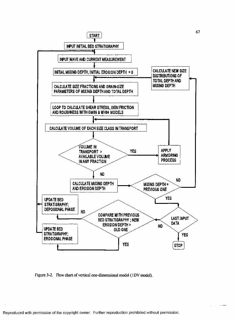
( START ] 67

YES

MIXING DEPTH = PREVIOUS ONE

YES

COMPARE WITH PREVIOUS BED STRATIGRAPHY; NEW

EROSION DEPTH >OLD ONE

LAST INPUT DATA

YESYES

VOLUME IN ^ TRANSPORT > AVAILABLE VOLUME IN ANY FRACTION

STOP

APPLYARMORINGPROCESS

INPUT INITIAL BED STRATIGRAPHY

INPUT WAVE AND CURRENT MEASUREMENT

INITIAL MIXING DEPTH, INITIAL EROSION DEPTH = 0

CALCULATE MIXING DEPTH AND EROSION DEPTH

UPDATE BED STRATIGRAPHY; DEPOSIONAL PHASE

UPDATE BED STRATIGRAPHY; EROSIONAL PHASE

CALCULATE VOLUME OF EACH SIZE CLASS IN TRANSPORT

CALCULATE NEW SIZE DISTRIBUTIONS OF TOTAL DEPTH AND MIXING DEPTH

LOOP TO CALCULATE SHEAR STRESS, SKIN FRICTION AND ROUGHNESS WITH GM86 & WH94 MODELS

CALCULATE SIZE FRACTIONS AND GRAIN-SIZE PARAMETERS OF MIXING DEPTH AND TOTAL DEPTH

Figure 3-2. Flow chart of vertical one-dimensional model (1DV model).


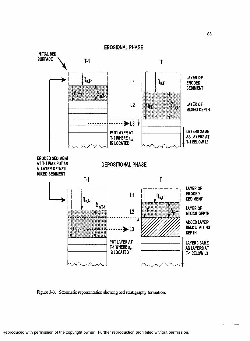
68

EROSIONAL PHASEINITIAL BED SURFACE

\ 1

A t-i

K ta

L1

L2

> L 3PUT LAYER AT T-1 WHERE n.T IS LOCATED

LAYER OFERODEDSEDIMENT

LAYER OF MIXING DEPTH

LAYERS SAME AS LAYERS AT T-1 BELOW L3

ERODED SEDIMENT AT T-1 WAS PUT AS A LAYER OF WELL MIXED SEDIMENT

DEPOSITIONAL PHASE

LT-1

< " -5

s i

- i

-r !

1t

cr |

------------H

F

L1

L2

> L 3

PUT LAYER AT T-1 WHEREillT IS LOCATED

ji

LAYER OFERODEDSEDIMENTLAYER OF MIXING DEPTHADDED LAYER BELOW MIXING DEPTHLAYERS SAME AS LAYERS AT T-1 BELOW L3

Figure 3-3. Schematic representation showing bed stratigraphy formatioa


69

depth; at the first cycle there is no difference in these parameters.

4) Calculate shear stress, skin friction, roughness parameters, and friction factor using the Grant and

Madsen (1986) model and ripple roughness using the Wiberg and Harris (1993) model.

5) Calculate the volume o f suspended load and bedload sediment.

6 ) Compare the potential o f sediment entrainment to the availability of the sediment imposed by the

total depth and if there is a shortage of sediment availability in any size class, then adjust

reference concentration to have the potential of sediment transport equal to the amount o f the

sediment available for transport (armoring process).

7) Calculate the erosion depth and new mixing depth based on the new size distribution in the mixed

layer.

8 ) Compare new mixing depth with the previous one, and until convergence, repeat procedures from

(3) through (8 ).

After finding a mixing depth, the procedure goes into the outer loop in which the new bed

stratigraphy (at time t) is made using the bed stratigraphy at time M . Figure 3-3 illustrates the

method used to construct the new stratigraphy. Depending on the result of the comparison between

the new erosion depth and the previous one, the procedure is diverted into an erosional phase or into

a depositional phase. The first layer from the initial bed surface (LI) is made by settlement of the

volume of sediment in transport. The second layer (L2) includes mixing depth at time t. Both LI and

L2 consist of the total depth, t ^ , and there is no difference between the erosional phase and the

depositional phase in constructing these two upper layers. At this point, the total depth plays a

significant role in the construction of the third layer (L3). During the erosional phase, the sediment

from the previous bed above the total depth at time t is transferred and redistributed into layers LI

and L2. Below the total depth in the previous bed, one layer may be a partial remnant. This remnant

is put into L3 in the new stratigraphy. The layers below L3 are identical to those of the previous bed.


70

During the depositional phase, the total depth will be located somewhere in the mixed layer of the

previous bed. In this case, the layer t\ t ., - r|a in the mixed layer is transferred into L3. When the

total depth is located above the bed surface, not shown in Figure 3-3, the whole mixed layer and the

layer t t_, - are put into L3 and then a mixing process is applied to make a homogeneous layer.

After this procedure, the new bed stratigraphy is used as an input for the next time step.

The common operations in the procedure to update bed stratigraphy are; (1) the

determination of the sediment size distribution in a given bed thickness, (2 ) the parallel

transformation of a single layer or a group of layers, (3) the division of a layer, and (4) the addition

of two layers. The first operation is performed using equation (3-51). The second and third

operations are straightforward and there is no change in the sediment size distribution. The number

of layers in the bed stratigraphy increases due to the second operation. However, the fourth operation

eliminates one layer and involves the mixing process which is similar to the first operation. Frequent

usage of the division and addition operations can cause physically unrealistic thin layers. An arbitrary

operation, basically operation 4, can be implemented to eliminate the thin layers. In the model

developed here, the minimum thickness of a bed layer is 0 .0 1 cm.


3-8. Results and Discussion

Input parameters describing flows include wave characteristics and a current specification

including current velocity magnitude and direction at a reference height for use by the Grant and

Madsen (1986) model. Input parameters describing the bed are rather complicated because the model

deals with multiple grain size classes as well as bed stratigraphy. Since bed stratigraphy is

characterized by the thickness and the grain size distribution of the bed layers, we need a two-

dimensional data (matrix): one dimension represents the bed thickness and the other represents the

grain size distribution. As a simple form, the bed stratigraphy presented in Figure 2-8 was used.

The resuspension coefficient y0 was the only tuning parameter to adjust the calculation of

suspended sediment concentration. The resuspension coefficient was iteratively adjusted until the

model predictions of suspended sediment concentration agreed with field measurements from 10 to

20 October 1994 at the 20 m depth (Fig. 3-4). It was possible to find a good agreement between

model predictions and field measurements using y0= 0.001. However, it was not possible to have

good agreement between the measured and predicted suspended sediment concentration at the 12 m

depth (Fig. 3-5). Especially predicted suspended concentrations were as twice as the measured

concentrations at higher three elevations during the storm peak. The poor agreement at the 12 m

depth may be attributed to the quality of the inshore OBS measurements as mentioned in Chapter 2.

The resuspension coefficient y0 is the essential parameter in predicting suspended sediment

concentration (see equation 3-32). This parameter has been estimated from many field experiments

and showed variability over several orders of magnitude. Smith and McLean (1977) estimated y0 =

2.4 x 10' 3 using field data from the Columbia river. The estimated resuspension coefficients on the

California shelf ranged from 1.5 x 10' 5 to 3 x 10"4 and these values were inversely proportional to

excess bed shear stress (Drake and Cacchione, 1989). They suggested two possible mechanisms for

this decreasing trend of y0 values with excess bed shear stress. (1) Due to bed armoring, bed


72

0 .8

120 cm ab0.6

0.4

++0.2

93 cm ab0.6

^ 0.4 CT)cT 0.2 O

c0 )ocoo

33 cm ab

0.5

2.5 7 cm ab+ +

+ + ++ + ++ +

0.5

10 12 14 16 18 20Days from 1 October, 1994

Figure 3-4. Predicted suspended sediment concentrations (solid line) are compared with field measurements (plus signs) at 20 m depth. The resuspension coefficient is y0 = 0.001.


73

119 cm ab

++

101 cm ab

O).-H-++Co

(D

c<Docoo

- ^ I . + i + , * ^ + + + t Ht :

36 cm ab

++

++ +4- +++ ^


Figure 3-5. Predicted suspended sediment concentrations (solid line) are compared with field measurements (plus signs) at 12 m depth. The resuspension coefficient is y0 = 0.001.


concentration Cb may not be a constant Since fine-grained sediment is winnowed into suspension

during early low-energy to medium-energy flow conditions, the fine fractions are depleted in the

surface layer of bed during high energy flows. This change in the bed concentration can lead to low

Yo values. (2) The grain cohesiveness beneath the loose surface sediment can cause change in critical

shear stress and erosion rate. This may also lower the Yo values. Vincent et al. (1990) showed the Ye

s ’ relation similar to that suggested by Drake and Cacchione (1989) but the estimated y0 values were

an order of magnitude larger. They suggested that the variation of Yo was related to wave-induced

ripples. Kim (1991) and Li et al. (1996) also showed that the strong vortex activity near the seabeds

due to wave-generated ripples caused the resuspension coefficient to have a higher apparent value

under low-energy fair-weather conditions. Under storm conditions, ripples were washed out with the

increase of bed shear stress and this reduced vortex activity, resulting in lowering y0 values to order

of 10"4. Under an extreme storm at the Duck site during the 1991 Halloween storm, Madsen et al.

(1993) obtained y0 = 4 x I O'4 for sheet flow conditions.

Hill et al. (1988) suggested a constant resuspension coefficient Yo = 1-3 x lO"4 based on

laboratory experiments and argued that the y0 - S relation shown in most field experiments may

result from improper treatment of the eddy diffusion coefficient or measurement errors. As Xu

(1993) noted, the effects of stratification and multiple sediment composition in suspended sediment

concentration complicated the inverse calculation of the resuspension coefficient using field

measurements even if he assumed a constant resuspension coefficient. In this study, bed

concentration for an individual size class is not a constant as that mentioned in the above field and

laboratory experiments in the above. This does not allow a simple y 0- S relation because both f C b

and S, in equation (3-32) are variables in association with flow conditions. Thus, the solution

procedure have to use a preset y0 value. Since f Cb depends on bed stratigraphy of the previous time

step, it is difficult to calculate inversely the resuspension coefficient at a certain time step using


75

concentration measurements. Therefore, we assume that y0 is a constant over flow conditions but

consider f C b as a variable. This may suggest that deviations between model predictions and field

measurements o f suspended sediment concentrations are attributable to this constant resuspension

coefficient. The iteratively estimated y0 value as the tuning parameter in the model is an order of

magnitude larger than those values obtained in storm conditions but it is close to the y0 value

suggested by Smith and McLean (1977).

The OBS measurements from 12 to 15 October at the lower two elevations (z = 7 cm and 33

cm) show poor agreement with model predictions of suspended sediment concentrations (Fig. 3-4).

There are several possible explanations for these deviations. First, Figure 3-6 shows predicted ripple

height from 10 to 20 October at the 20 m depth. The predicted ripple height was about 2 cm at the

beginning and it decreased with the increasing wave orbital velocities (see Fig. 2-6). Ripples were

washed out during strongest flow conditions from 15 to 17 October. After this period, ripples were

regenerated for two days as flows were weakened. They disappeared again on 19 October when wave

orbital velocities increased moderately. This disappearance may be due to either the increased wave

orbital diameter induced by swells or the decreased sediment size. Since the sediment size of the top

1 cm thick bed was not significantly changed (see Fig. 3-15 b) during the waning storm phase at the

20 m depth, ripples were washed out by swells. The model indicated existence of ripples during the

period of poor predictions and vortex action due to ripples may have enhanced resuspension of

sediment. The diffusion model used in this study probably underestimates suspended sediment

concentrations because it doesn’t include the vortex action due to ripples. Alternatively, the actual y0

value may be larger than the constant y0 value used in the model. A diffiision-advection model is

capable to deal with the effects o f vortex action on resuspension o f sediment as suggested by Nielsen

(1993).

A second source of the poor agreement may be that the model ignored possible contribution


76

V ,

O)

8 - 0.8

0.6

0.4

0.2


Figure 3-6. Predicted ripple heights show that ripples disappear during sheet flow conditions.


77

caused by the spatial gradient o f sediment flux in the sediment conservation equation. This will be

discussed in Chapter 4. Additionally, malfunctions of OBS sensors can cause some damage to the

data quality. As shown in Chapter 2, the apparently incorrect data in Figure 2-8 b were removed.

There may exist some drift in the truncated OBS data which may start at an early stage of the storm.

The lowest OBS sensor, positioned at 7 cm above the bed, shows obviously a sudden jump of OBS

data right after 12 October while the OBS data of other four sensors change little (Fig. 2 - 8 b). This

indicates the small drift of the lowest OBS sensor. Considering overall time series of the OBS data,

all sensors have some drift problem. The upper two OBS sensors (sensor 4 and 5) appear to have

smaller drift than the lower three OBS sensors (sensor 1 to 3). This may result in better agreement

between model predictions and field measurements of concentrations in the upper two OBS sensors

than the lower sensors (Fig. 3-4). However, these small drifts are difficult to remove because these

are not explicitly separated from the correct signal.

An interesting feature o f the model predictions in Figures 3-4 and 3-5 is the asymmetric

variation of the suspended sediment concentration in response to the more or less symmetrical

variation of flow conditions with time (see Fig. 2-6). Suspended sediment concentrations during the

erosional phase (October 10-16) were smaller than those during the depositional phase (after

October 16). Unfortunately, the truncated OBS measurements could not support the behavior of the

model predictions during the waning storm phase. This kind of behavior of the suspended sediment

concentration was observed in other field experiments (Shi et al., 1985) and interpreted as hysteresis

effects which were related to time-dependent processes. Wiberg et al. (1994) noticed that steady

models can underestimate suspended sediment concentrations during waning flows because the

sediment suspended at peak flow conditions is neglected between calculation time steps. They

suggested that time-dependent effects should be considered in steady models to improve model

predictions. The model developed here satisfies two conditions for steady models as described in


78

Wiberg et al. (1994): (1) suspended sediment concentrations are in equilibrium with the imposed

flow and (2) the bed is well-mixed at all times. The difference of this model from most steady

boundary layer models is to take care of the contribution of sediment suspended at high flow

conditions through the total depth T |t which is related to the sediment availability for resuspension.

Also, the armoring process may be responsible for this model behavior rather than time-dependent

processes. During an erosional phase, the amount of sediment in suspension is less than the capacity

of the flow to suspend sediment because the coarse-grained armored layer prevents the erosion of the

fine-grained sediment This means that the bed controls the suspended sediment concentration during

the resuspension period. On the contrary, the armoring process ceases during the depositional phase

and thus the capacity of the flow to suspend sediment plays an important role in governing the

suspended sediment dynamics. Therefore, flows reaching equilibrium with resuspended sediment can

support higher concentrations.

The model also predicted the shear velocity due to the current above the wave boundary layer

and the apparent roughness. The comparisons of the predicted values with the field measurements of

these parameters are presented in Figure 3-7 and Figure 3-8. The field measurements of both shear

velocity and apparent roughness at the 20 m depth agree well with model predictions (Fig. 3-7). The

field measurements of these variables at the 12 m depth showed very poor agreements with the

predicted values (Fig. 3-7). Again, the poor quality of field measurements at the 12 m depth was

responsible for discrepancies mainly because only three measured values were involved in the

calculation of the velocity profile.

Comparison of the predicted u.c and zM values between the two locations showed similar

variation with time. Also, the magnitudes of predicted values from the two locations were similar. So

it can be said that shear stresses due to currents were quite similar at both sites. But there was

significant difference in the model predictions of suspended sediment concentrations (Fig. 3-4 and 3-


79

(a)

(b)

5

4 + +

o<D o (OEo

1

0

cooN

10

o10

++ + ++ + +'

•1++10

•210

-310


Figure 3-7. Predicted values of shear velocity (a) and apparent roughness (b) are compared with field measurements at 20 m depth. Solid lines represent the model predictions and plus signs represent the field measurements.


80

(a)

(b)

++

-H-

++,

+ .+ ++

£

to oN

10: +++

o10

-H-

■110

■210


Figure 3-8. Predicted values of shear velocity (a) and apparent roughness (b) are compared with field measurements at 12 m depth. Solid lines represent the model predictions and plus signs represent the field measurements.


81

5). The predicted values at the 12 m depth location were two to three times greater than those at the

20 m depth location. Considering the higher wave-orbital velocities at the 12 m depth (Fig. 2-11),

waves were the main agents agitating the bottom sediment as observed in Wright et al. (1986; 1991).

To examine the effects of coupling between the boundary layer process model and bed

stratigraphy on the prediction of hydrodynamic and sediment transport parameters, a decoupled

model was constructed and its predictions were compared with the coupled model predictions. The

decoupled model was different from the coupled model in a few respects; it did not account for the

armoring processes or changes of the bottom sediment with time. Since the armoring process is not

separable from the process of changing bottom sediment from the theoretical point of view,

comparison o f the two models indicated combined effects of the couplings. Predicted values of

suspended sediment concentrations at the 2 0 m depth from both coupled and decoupled models are

compared in Figure 3-9. It shows that the decoupled model overestimated the suspended sediment

concentration at the time of the storm peak from 15 to 16 October. Except at the time of the storm

peak, both predicted values were not significantly different. The overestimation of the decoupled

model is attributable to the resuspension coefficient y0 = 0 .0 0 1 which is too high for sheet flow

conditions. Adjustment of the decoupled model to use other y0 values is required.

To adjust the decoupled model the y0 value was lowered to 4 x lO"1 which was suggested by

Madsen et al. (1993) with the reference concentration calculated at the height z = 7 d50 for sheet flow

conditions. As shown in Figure 3-10, except at the lower two elevations, the decoupled model

overestimates at the upper two elevations during the storm peak. Predicted values of both the coupled

and decoupled models are comparable during low energy conditions. In an attempt to improve

predictions o f the coupled model at higher elevations, the y0 value was lowered to 2 x 10"4 (Fig. 3-

11). But this caused underestimation at lower elevations during the storm peak. During the low

energy conditions, the decoupled model predicted much smaller concentration than the coupled


82

model. Based on these two analyses, one may choose an intermediate y0 value between 2 x lO"* and 4

x I O'4 to compromise the adverse results caused by these two y0 values. When the resuspension

coefficient is taken as Yo = 3 x 1 0"4, the decoupled model overestimates at higher elevations and

underestimates at lower elevations during the sheet flow conditions (Fig. 3-12). This can be seen in a

concentration profile (at Hour 12 on 15 October) in which the decoupled model gives a gentle

concentration profile compared with the coupled model (Fig. 3-13). As we have attempted to adjust

the decoupled model using several values of the resuspension coefficient (Fig. 3-10 to 12), slopes of

predicted concentration profiles will be consistent between these different values. This gentle slope

may be an intrinsic nature of the concentration profile predicted by the decoupled model. This

demonstrates that it is difficult to get good agreement between decoupled model predictions and the

OBS data.

The underestimation at lower elevations by the decoupled model probably results from low

coarse-grained sediment composition in suspended sediment because of low y0 value. In the coupled

model, however, coarse sediment is enriched on the bed surface as an armored bed is developed. This

coarsened surface layer provides large amount of coarse sediment to be suspended. This contributes

high concentration at lower elevations but low concentration at higher elevations because the settling

velocity of the coarse sediment is large. This results in a steep concentration profile. Contrary to the

coarse sediment situation, fine-grained sediment has small settling velocity and gives a gentle

concentration profile. Fine-grained sediment contributes more effectively to suspended sediment at

higher elevations than coarse sediment Since there is no constraint for the erosion o f fine-grained

sediment in the decoupled model, the bed supplies large amount o f fine-grained sediment to the water

column. Therefore, the overestimation at higher elevations is likely attributable to fine-grained

sediment as the degree o f overestimation increased at higher elevations. However, an armored layer

limits the supply of fine-grained sediment and results in low concentration at high elevations in the


83

oCM

iCO

coXi(0

EoN-

t

< +

i CM

OOCO CO CM

OCM

00

JO(0

EooCM

COncoEoCOCOoo

o '

CM

oCO O M- coCM

(1/6) uojjejjuaouoo (|/6) uo!jBj;uaouoo

Figure 3-9. Suspended sediment concentrations predicted by coupled model (solid line) are compared with those predicted by decoupled model (dashed line) when the Yo value of the decoupled model is y0 = 0.001. Plus signs represent the OBS data at 20 m depth.


Days

fro

m 1

Oct

ober

, 19

94

Days

fro

m 1

Oct

ober

, 19

94

84

oCM

CO

CO-QCO

EoCOCD

XICOEo[•»

om o in om inO CM T-‘ o'

oCM

CO

X!CO

EooCM

XCO

EoCOCO

oooo'

CM

3 o O'r-m m O CM m

o' T-' o'(l/6 ) uo!1B j;u 0 O u o q ( |/6 ) u o j jB J iu e o u o o

Figure 3-10. Suspended sediment concentrations predicted by coupled model (solid line) are compared with those predicted by decoupled model (dashed line) when the y0 value of the decoupled model is y0= 0.0004. Plus signs represent the OBS data at 20 m depth.


Days

fro

m 1

Oct

ober

, 19

94

Days

fro

m 1

Oct

ober

, 19

94

85

CD CO o>

_QCOEo

CO05

XICDEoD-

CM

OCO CO m in oo’ o’ o’ o’ cn t- o’

CO CD

JOCDEooCN CO

COoo

CN

COo'

CO N-o

CN O CN in ino ’

o

(1/ 6 ) u o i j e j j u e o u o o ( |/6 ) u o u e j j u a o u o o

Figure 3-11. Suspended sediment concentrations predicted by coupled model (solid line) are compared with those predicted by decoupled model (dashed line) when the y0 value o f the decoupled model is y0 = 0.0002. Plus signs represent the OBS data at 20 m depth.


86

_QCD

EoCOO)

-QCO

Eoh-

[+'

o■M"o '

o in ino '

CD coo '

CM CM

CO

.QCO

EooCM

X ICO

EoCOCO

----COoooo'

o

oCOo'

O CMCO CM to

(1/ 6 ) u o !1B j;u 0 O u o q ( |/6 ) u o ! ;b j ;u 0 O u o q

Figure 3-12. Suspended sediment concentrations predicted by coupled model (solid line) are compared with those predicted by decoupled model (dashed line) when the y0 value of the decoupled model is Yo= 0.0003. Plus signs represent the OBS data at 20 m depth.


Days

fro

m 1

Oct

ober

, 19

94

Days

fro

m 1

Oct

ober

, 19

94

87

Hour 12,15 October

EocoCD>0 )LU

0.2 0.4 0.6 0.8 1 1.2 1.4 1.6 1.8 2Concentration (g/l)

Figure 3-13. Suspended sediment concentration profile predicted by coupled model (solid line) is compared with that predicted by decoupled model (dashed line) when the y0 value of the decoupled model is y0 = 0.0003. Plus signs represent the OBS data at 20 m depth. This shows that the coupled model predicts suspended sediment concentrations better than the decoupled model.


88

coupled model. This implies that the armoring process was critical to obtain a correct gradient of

concentration profile. In addition, it is noteworthy that the coupled model predicted higher suspended

sediment concentrations during the waning phase of the storm than the decoupled model.

In contrast to the difference presented in Figure 3-9, the predicted values for shear velocity

and apparent roughness from both models were too close to allow the effects o f couplings on the

hydrodynamic parameters to be differentiated (Fig. 3-14). Small grain size changes may result from

the sediment having a relatively narrow range of grain size distribution (i.e., well sorted). In other

environments such as a river channel, bottom sediment is composed of sand-gravel mixtures which

show a much wide range of grain size distribution and multiple modes. In that condition, grain size

changes in the bed surface can be anticipated to affect significantly the shear stress and roughness

parameters (Kuhnle, 1989). Apparently, the hypothesis that the changing bottom sediment affects the

hydrodynamics may not be useful for the boundary layer processes in inner-shelf environments.

Instead, these effects were most profound in sediment transport It implied that the model is still

useful. Small changes in the sediment size in the armored layer were very effective on sediment

transport but the shear stress terms. It can be said that a model showing good agreement with the

hydrodynamics doesn’t necessarily provide good predictions of sediment transport if it is not coupled

with bed stratigraphy. The fact that hydrodynamic variables can be accurately estimated without

couplings is very helpful in designing a complicated hydrodynamic model. A partly decoupled model

in the calculation of the hydrodynamics avoids time-consuming procedures.

In the following, model outputs, which have no field data to compare with, are presented. As

mentioned earlier, the acquisition of bed characteristics in field experiments is not easy. So there is

no way to calibrate and validate the model outputs using field data. Nevertheless, the validity of

model predictions of bed stratigraphy can be evaluated indirectly by comparison of the model

predictions of suspended sediment transport with field measurements on the basis that the model


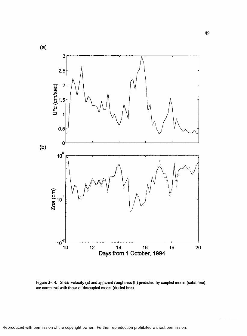
89

(a)3

2.5

2

1.5

1

0.5

0

o


Figure 3-14. Shear velocity (a) and apparent roughness (b) predicted by coupled model (solid line) are compared with those of decoupled model (dotted line).


90

couples the boundary layer processes with bed stratigraphy. As mentioned previously, a model

coupled with bed stratigraphy appears to be superior for the prediction o f suspended sediment

concentration. For this reason, it is proposed that the predicted bed stratigraphy may be valid, at least

qualitatively.

The model predictions of the length scales, erosion depth and mixing depth, and the grain

size parameters at both the 10 m and 20 m depths are presented in Figure 3-15 and Figure 3-16

respectively. The predicted length scales at both locations showed the same patterns that were closely

related to wave orbital velocities. The maximum erosion depth at the time of the storm peak was 0.5

cm at the 20 m depth and 2 cm at the 12 m depth. The increased erosion depth at the 12 m depth

reflected increased wave-current interactions. The time series of sediment size at both locations

showed the tendency that sediment size reached a maximum value during the storm peak and then

decreased to be finer than the initial values (Fig. 3-16). The maximum sediment size in the armored

layers at both locations was 2.5 $ and 2.8 (j) respectively. Some differences between the two sites

occurred during the depositional phase. The sediment size in the top 1 cm thick bed at the 20 m depth

did not change much after the model run but at the 12 m depth it decreased from 3 (j) to 3.5 (j). Since

the sediment became finer after the storm event at the 12 m depth, small ripples were expected. This

demonstrates that model predictions of sediment size were consistent with observations described in

Wright (1993). It seems that the model predicts qualitatively the roughness changes of seabeds in

response to storm events.

In Figure 3-17, the model predictions of the erosion depth using the decoupled model were

compared with values obtained using the coupled model when both models were adjusted by same y0

value, Yo = 0.001. At the time of the storm peak, the erosion depth predicted by the decoupled model

was 3 cm which is six times greater than that predicted by the coupled model. During low energy

conditions, both models predicted comparable results. When the resuspension coefficient of the


91

(a)

Q.

-1.5(b)

2.5

CL3.5

4.5


Figure 3-15. Model predictions of bottom sediment length scales and sediment size at 20 m depth, (a) shows the erosion depth (cross signs) and the total depth (star signs), (b) shows the median diameter of the mixed layer (circle signs) and that of the top 1 cm thick bed (plus signs).


92

(a)o ixxxxxxxxxxxxxxx&oc

0 -1

-4

2.5

Q.0 3.5

4.5

5.518 2010 12 14 16


Figure 3-16. Model predictions of bottom sediment length scales and sediment size at 12 m depth, (a) shows the erosion depth (cross signs) and the total depth (star signs), (b) shows the median diameter of the mixed layer (circle signs) and that o f the top 1 cm thick bed (plus signs).


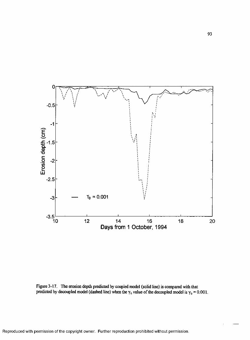
93

-0.5

"O

-2.5

Y0 = 0.001

-3.510 12 14 16 18 20


Figure 3-17. The erosion depth predicted by coupled model (solid line) is compared with that predicted by decoupled model (dashed line) when the y0 value of the decoupled model is y0 = 0 .0 0 1 .


94

»•

- 0.1

- 0.2

-0.3

-0.4

- 0.6

-0.7

- 0.8Y0 = 0.0003

-0.9


Figure 3-18. The erosion depth predicted by coupled model (solid line) is compared with that predicted by decoupled model (dashed line) when the y0 value of the decoupled model is y0 = 0.0003. During high energy flows, the decoupled model predicts the erosion depth as twice as the coupled model. This implies that the decoupled model has the potential to overestimate sediment transport.


95

decoupled model was lowered to 3 x I O'4, the erosion depth predicted by the decoupled model was as

twice as the coupled model during the storm peak (Fig. 3-18). Since the erosion depth equals to the

depth-integrated suspended sediment concentration, a steep concentration profile gives smaller value

of the erosion depth. The concentration profile calculated by the coupled model is steeper than that

calculated by the decoupled model (Fig. 3-13). Therefore, the decoupled model has the potential to

overestimate sediment transport during storm events.

The predicted bed stratigraphy at the 20 m depth is shown in Figure 3-19. The thickness of

storm deposit was predicted to be approximately 1.3 cm. This storm deposit showed fining upward

sequences. The base of the storm deposit consisted of the coarsest material. The median diameter of

the top layer was smaller than the initial sediment size. The size distributions of the individual layers

in the storm deposit are presented in Figure 3-20. It shows clearly a fining upward trend in a graded

bed. The layers 4 to 6 must be armored layers in that fine-grained sediment is depleted As for the

predicted bed stratigraphy at the 12 m depth, thicker storm deposits resulted from the high intensity

of wave orbital velocities (Fig. 3-21). Compared with the bed stratigraphy at the 20 m depth, the

base of the storm deposit was much coarser. To compensate for this coarsening, the top layer of the

storm deposit contained fine-grained sediment with the sand size fractions depleted as seen in Figure

3-22.

The observed bed stratigraphy is shown in Figure 2-4. Since this sediment core was analyzed

at 1 cm intervals, precise structures within the 2 cm thick layer which indicates fining upward trend

was not provided From this surface layer to about 5 cm depth of the core, sediment shows

coarsening upward trend The thin surface layer showing a fining upward trend is attributable to a

storm event. Variations below the surface layer may be related to long term processes including

bioturbation. In order to compare bed stratigraphy predicted by the model developed here with field

observations, it is necessary to collect sediment carefully focusing on the upper few centimeters of


96

-0.5

Q .

-2.5

o Median grain size in the layer

3 4 5 6 7 8 9 101 2Size class (phi)

Figure 3-19. Predicted bed stratigraphy at 20 m depth. Thickness of the predicted storm deposit is about 1.3 cm. The storm deposit shows a fining upward trend.


97

"i 1------------- 1--------------1------------- 1--------------1--------------1--------------r

^ 0 O•t?3CO0

3 SEo

0.aE3C1—0>»0

4 5 6 7Size class (phi)

8 10

Figure 3-20. Predicted grain size distributions of individual layers in the predicted bed stratigraphy at 20 m depth. Each layer in the bed stratigraphy is denoted by the numbers on the vertical axis. Number 1 represents top layer. Size distribution of layer number 7 equals to that of initial bed stratigraphy.


98

-0.5

~uroa .■o

-3.5

o Median grain size in the layer_ ^ i ________ i________ i________ i________ i________ i________ i________ i________ i________

1 2 3 4 5 6 7 8 9 10Size class (phi)

Figure 3-21. Predicted bed stratigraphy at 12 m depth. Thickness of the predicted storm deposit is about 3.5 cm.


99

<Uo- I3(0»(0

84 5 6 7

Size class (phi)8 10

Figure 3-22. Predicted grain size distributions of individual layers in the predicted bed stratigraphy at 12 m depth. Each layer in the bed stratigraphy is denoted by the numbers on the vertical axis. Number 1 represents top layer. Size distribution of layer number 8 equals to that of initial bed stratigraphy.


100

bottom sediment This sediment should not be disturbed to preserve micro-scale structures. Also, the

time to collect sediment samples after storm events is important because these are temporal

structures. Without these careful controls, comparisons between predicted bed stratigraphy and

observed sediment core will not be robust

3-9. Limitations of the Model

Several assumptions underlie the model and are sources of weakness when applying the

model to realistic field conditions. In the derivation of the sediment conservation equation, the

horizontal flux term was dropped. This is not always justified in the inner-shelf environment where

across-shelf transport induces morphological changes during high energy events (Wright et al.,

1991). But the lack of data concerning this spatial term makes it difficult to include the horizontal

flux term.

The assumption of a steady state introduces errors regardless of the time scale and interval

used. For example, suspended sand has a relatively short response time to changes of flows because

of its large settling velocity. The response time increases as the sediment size decreases. In spite o f

the fact that fine-grained sediment is a small fraction of the total composition of the inner-shelf

sediment, it is a large fraction of suspended sediment and can cause significant effects on the OBS

measurements. OBS sensors are more sensitive to fine-grained than coarse-grained sediment

(Ludwig and Hanes, 1990; Green and Boon, 1993). Predicting the behavior of the fine-grained

sediment accurately requires a time-dependent model.

The model mainly focuses on the physical processes, the relationship between the sediment

transport and bed responses, during a resuspension event. This makes it of limited applicability to the

fair-weather period when the biological mixing process dominates. So the time scale of the model is

limited to the range of hours to days which is long enough to cover a high energy event. Biological


101

activity may be so efficient during a calm period that the sedimentary structures of the surface layer

can be destroyed in a time scale less than one day (Myers, 1977; Grant, 1983). Including fair-weather

processes into a long term model such as that developed by Harris (1994) would be a virtual pursuit

but beyond the scope of this study. Also, the model in this study results in one unit of bed

stratigraphy, a graded bed, whose thickness is in the order of mm to cm (Niederoda et al., 1989).

This range of the bed thickness is not comparable to a geological stratigraphic unit.

The wave-current interaction model of Grant and Madsen (1979; 1986) has been

successfully applied to the inner-shelf environment It is based on a time invariant eddy viscosity

which increases linearly in the lower wave boundary layer as well as in the upper current boundary

layer, but has a discontinuity between two layers. Consistent with this eddy viscosity profile, a Rouse

type equation has been used to predict suspended sediment concentrations (Drake and Cacchione,

1989). When wave-generated ripples occupy the seabeds, it was observed that vortex ejection from

the bedforms causes variation of concentration profiles (Vincent et al., 1991; Nielsen, 1993). They

deviate from the predictions of the simple diffusion model.

Another limitation is that the model assumes noncohesive sediment and cohesive properties

are assumed to be minor. In cohesive sediment transport, thresholds of erosion are different from

those of deposition. However, this differentiation in noncohesive sediment is not taken into account

because erosion and deposition occur at the same time (Sanford and Halka, 1993). Combining these

two processes may be necessary in a time-dependent numerical model. So it is reasonable to apply

the model developed in this chapter to an environment where cohesive properties in the sediment are

not significant


4. ACROSS-SHELF TRANSPORT: 1DH DEPTH-RESOLVED MODEL

4-1. Introduction

Across-shelf sediment flux on the inner continental shelf involves numerous processes

(Swift et al., 1985; Wright et al., 1991). Tide induced and wind-driven currents are relatively more

important on the inner shelf than in the surf zone. The significant role of mean currents for advective

transport has been recognized. For engineering applications within surf zones, Dean (1991) applied

simple equilibrium beach profile concepts to profile changes. Equilibrium profiles were constructed

based solely on considerations o f wave dissipation and with the unrealistic assumption of a shallow

depth of closure beyond which there is no sediment movement. During disequilibrium, cross-shore

sediment transport is assumed to occur by a diffusive process and unidirectional currents are not

considered (Pilkey et al., 1993). Wave-induced bed shear stress is considered to entrain sediment

particles but to contribute little to advective movement. In nature, mean currents are responsible for

cross-shore sediment flux although their magnitude is much smaller than that of wave orbital

velocities. Therefore, to extend such simple equilibrium concepts to inner shelf without considering

currents would be unrealistic.

It has been noted that the direction of sediment transport depends strongly upon mean

currents (Wright et al., 1991). Also, asymmetrical wave orbital velocities promote shoreward mass

transport (Swift et al., 1985). With a sloping plane bed, equilibrium is attained when there is a

balance between onshore sediment flux due to asymmetrical orbital velocities and down-slope

gravitational flux. This profile is attacked by storms which generate intensified wind-driven

102


103

circulations. On the middle Atlantic shelf, wind stress is commonly onshore during storms. The rates

of offshore sediment transport due to strong downwelling mean currents can be an order of

magnitude greater than onshore transport by fair-weather swells (Wright et al., 1991). Niederoda et

al. (1985) interpreted a cross-shore deficit of inner-shelf sediment budget on the basis of geological

time scales with a sea level rise as an important factor affecting the erosional retreat of barrier islands

along the east coast of the United States.

Relative rates o f cross-shore sediment transport, with regard to steady currents, incident

waves, long-period infragravity waves and the gravitational component caused by a sloping bed,

were obtained from a sediment transport model (Bailard, 1981) based on Bagnold's energetics model.

The predicted values were not consistent with observed values except in terms of the qualitative

direction o f each component (Wright et al, 1991). Mean flows were found to dominate observed

cross-shore sediment flux in all conditions. While high-frequency waves were predicted to be

significant in all conditions, they were observed as a major mechanism for shoreward sediment

transport only during swell-dominated conditions. Since energetics models are based on

instantaneous velocities, it was impossible to represent the phase relationship between the maximum

near bottom velocity and the maximum concentration of suspended sediment under fair-weather and

moderate wave energy conditions. However, both quantities were in phase under high energy

conditions, i.e., storms. Wright et al (1991) suggested that the discrepancies corresponding to low

and moderate energy conditions may be attributed to the presence of wave-generated ripples.

To take the horizontal flux term into consideration, we need to know the flow field. During a

storm event, wind may be the dominant force driving circulation on the inner shelf, but wave and

Coriolis forces are not negligible. Here, these three terms are included to derive a simple analytical

solution o f the two-dimensional equation of motion following the Jenter and Madsen model (Jenter

and Madsen, 1989; Chisholm, 1993; Madsen et al., 1994). In this chapter, the appropriate


104

hydrodynamic models are implemented in a horizontal one-dimensional model scheme (1DH model)

in order to investigate the wind-driven processes for the erosion/deposition of the inner-shelf

morphology. Components of this model are shown in Figure 4-1. Assuming a simple geometry in

which along-shelf variation is negligible, a one-dimensional set of grids was constructed in the

across-shelf direction. Based on this simple geometry, simple wave transformation is used to

calculate wave fields. Using the computed waves and the input of winds, current profiles at each grid

point were predicted by the Jenter and Madsen (1989) model which is coupled with a wave-current

interaction model. Depth-integrated sediment flux was estimated using the predicted hydrodynamics

and bed stratigraphy in association with fractional transport and armoring processes. The horizontal

flux divergence was numerically solved to yield bed elevation changes related to individual size

classes.

4-2. Wave Transformation Model

4-2-1. Formulation

Assuming a simple geometry consisting of straight and parallel contours, wave

transformation along wave rays on the inner shelf can be predicted to the lowest order using simple

linear wave theory which is described in Dean and Dalrymple (1992). Assuming that the wave energy

is conserved and neglecting reflection, diffraction and frictional dissipation, the wave height H, at

intermediate or shallow water (at x = 1) can be determined by

H, = f f0 Ks Kr (4-1)

where H0 is the wave height at deep water (at x = 0), Ks is the shoaling coefficient and Kr is refraction

coefficient The shoaling coefficient Ks is given by


105

INPUT WAVE

INPUT WIND

1D GEOMETRY

SEDIMENT FLUX

CURRENT MODEL

BED STRATIGRAPHY AND BED ELEVATION

WAVE TRANSFORMATION MODEL

Figure 4-1. Flow chart of horizontal one-dimensional, across-shelf sediment transport model.


106

N 2Cgi(4-2)

where Ca is the deep water wave celerity (L /T) and Czi is the group velocity at x = 1. The wave

numbers at both locations are calculated by Hunt’s approximate equations (2-5) and (2-6) and also,

The refraction coefficient Kr can be determined directly provided the assumption of straight,

parallel contours is valid,

where b0 and b, are the distance between the wave rays at locations 0 and 1 respectively and 0 O and

0, are the incident angles at x = 0 and 1, made by the wave ray and the across-shelf x axis. Except

where contours protrude seaward (convex seaward), this refraction coefficient is always smaller than

unity. The incident angle at x = 1 is calculated using Snell’s law which is

Cj = C0 tanh kh (4-3)

With the wave speed Ch the group velocity at x = 1 is given by

(4-4)

sinOj sin0 o(4-6)C C

'■ ' l ' - ' o

Considering the effects of real sea beds, wave damping due to bottom friction becomes


significant as waves propagate into shallow water and may reduce the wave height (Liu and Tsay,

1985; Maa and Kim, 1992). The average rate of the energy dissipation related to the rough turbulent

boundary layer can be formulated as

6 d = Tbu b = f e u l ( 4 ' 7 )

where tb is the maximum bed shear stress, ub is the rms bottom orbital velocity, p is water density

and f t is Jonsson’s (1966) wave friction factor. The energy flux equation leads to

dECi f ' - e° (4-s >

Inserting E=(l/8)pgI-P and equation (4-4) into (4-8), we get (4-9) after some manipulation.

dH2 V e { cof c ~ 37i g e l sinh kh) (4‘9)

It is noted that (4.9) can be applied only to a flat bed. Solving (4.9) for the wave height with the

boundary condition, H0 at x = 0, we have

1- = * / =H0 J i 4/e k 2 H0 x (4.10)

3n (2kh + sinh 2kh) sinh kh

where x is the traveling distance in the wave propagation direction. The damping coefficient can

be included in (4-1) leading to

H ^ H , K s Kr Kf (4 - 1 1 )


108

To apply (4-10) to a gentle slope bottom, the bottom of each segment of grids is assumed to

be a flat bed and then the damping coefficient Kf is calculated locally along the wave ray. In addition,

the distance at each segment which a wave propagates depends on the wave incident angle 6 and it

can be roughly expressed as r/cos0. The effects of wave damping along a refracting wave ray are

thus cumulative.

The friction factor in (4-10) is the only unknown and it must be determined using field

measurements. Using Swart’s formula (Swart, 1974), which is a function of the roughness kb (=30z0)

and the semi-excursion amplitude Ab, the friction factor f is given by

f e = exp

0.194k .

5.213 b - 5.977Ab

k.fo r -2. < 0.63

A,.(4-12)

f e = 0.3 fo r - ± > 0.63Ab

For simplicity, the roughness kb is considered to be a constant through the comparison with field

measurements although it varies with time and space.

5-2-2. Determination of Wave Friction Factor

The FRF wave data measured at 8 m and 17 m depths were used to determine the friction

factor of the wave transformation model. Wave heights during October 1994 reached 4 m and

included three events where wave height exceeded 1 m (Fig. 4-2 a). Comparison of model predictions

with field measurements mostly used the broad peak of wave heights from 10 to 20 October. The

time series of the difference between the wave heights at the two locations (Fig. 4-2 b) appeared to be

proportional to the magnitudes of the wave heights and tended to be positive except during the period

from 16 to 21 October. The positive difference means that the wave height in shallow water is


109

smaller. Several factors may have caused the changes of the wave height along the across-shelf

transect The inner shelf is where wave transformation due to shoaling and refraction occurs and also

the wave dissipation due to friction or input from a wind source is possible. These processes depend

on wave and wind conditions. As discussed in Battjes et al. (1990), we need to investigate the effect

o f whitecapping which may be responsible for wave dissipation in an actively wind-driven wave

field.

To begin with, the wave transformation model was run using (4-1), assuming that there was

no dissipation of the wave energy flux. The model predictions of the wave heights were compared

with the field measurements (Fig. 4-3). In general, good agreement occurred for high energy waves

and long-period waves (not shown here). During the period when the wave height was less than 1 m,

for example, from 5 to 10 October, wave heights were not predictable and probably depend on wind

conditions. However, the wave transformation during the period of high energy waves, from 10 to 20

October, was strongly governed by the wave period. As seen in Figure 4-4, the errors between the

model predictions and the field measurements (Fig. 4-3) appeared to follow the trend of wave periods

rather than that of wind speeds. Dissipation of the wave energy flux, objecting the assumption, was

responsible for these errors. Wave dissipation due to friction depends on the wave period. Therefore,

we could apply a wave damping factor to the model to improve predictions of the wave height

variations with changing depth. The simulation produced by the wave transformation model is

presented in Figure 4-5, using the adjusted roughness parameter kb = 0.1 cm. There has good

agreement between the model predictions and the field measurements during the period of the high-

energy and long-period waves.


110

(a ) FRF W ave;-17m -8m

60

Eo ,

X 20 ■

n -T“I

-2010 15 20 25Days from 1 October, 1994

Figure 4-2. The FRF wave heights measured at 8 m (dashed line) and 17 m (solid line) depths in October 1994. (a) shows time series of the wave heights (in the m unit), (b) represents difference (in the cm unit) between the wave heights at the two locations and this shows a tendency that the wave height at the 8 m depth is smaller.


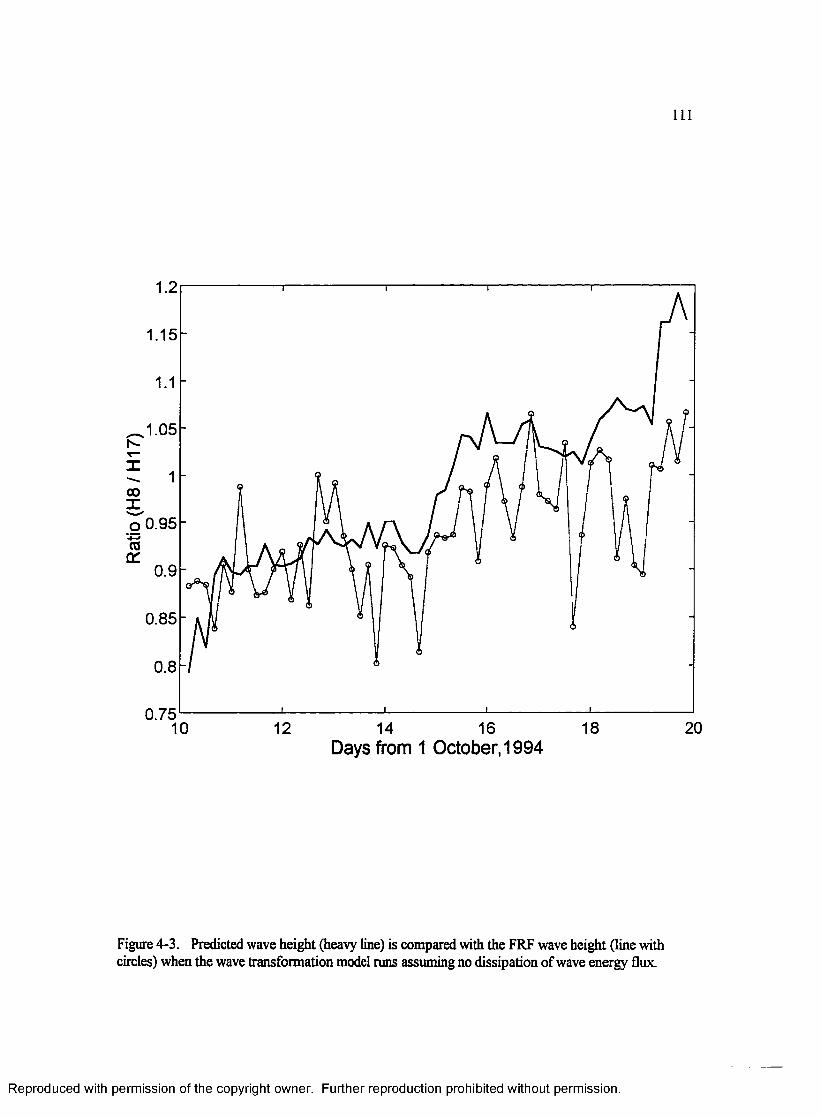
I l l

1.2

1.15

.05

GO

o 0.95

0.9

0.85

0.8

0.7518 2010 12 14 16


Figure 4-3. Predicted wave height (heavy line) is compared with the FRF wave height (line with circles) when the wave transformation model runs assuming no dissipation of wave energy flux.


112

(a)

20(b)

<0 10

20(C)

•o0 10 d)Q.

T3


Figure 4-4. Errors (a) between model predictions and field measurements of wave height are compared with wave period (b) and wind speed (c ).


Ratio

(H

8/H

17)

113

kb= 0.1cm ; -o- measured, - predicted1.2

1.15

1.05

0.95

0.9

0.85

0.8

0.7510 12 14 16 18 20


Figure 4-5. Predicted wave height (heavy line) is compared with the FRF wave height (line with circles) when the roughness parameter kb is 0 .1 cm.


114

4-3. Current Model

4-3-1. Formulation

The current model used in this study is described in Jenter and Madsen (1989), Poon and

Madsen (1991), Chisholm (1993) and Madsen et al. (1994). The momentum equations o f a depth-

resolving hydrodynamic model for a steady, linear, inviscid, and homogeneous water column in

horizontal x-y plane are given by

" A = - g ^ + (4-13)etc p az

/ “ = -grj*- + (4-14)ay p az

where/is the Coriolis parameter, g is the acceleration of gravity, p is the water density, £ is the sea

surface elevation, z is the vertical coordinate, u and v are the local velocity components in the x andy

direction, and t x and Ty are the turbulent Reynolds’ stresses. The turbulent stress profile depends on

the eddy viscosity v, and velocity shear

and the eddy viscosity, following Madsen (1977), is

v, = fo r 0 < z < zm(4-16)

= K u jh -z ) fo r zm < z < h

where k = 0.4 is von Karman’s constant, h is the water depth, and zm is defined as


115

z_ = h ± (4-17)u + u .•s *6

in which = yjxjp and = J x jp are the shear velocity on the bottom and surface boundary

respectively.

Inserting (4-15) into (4-13) and (4-14), then multiplying (4-14) by/ = , and adding to

(4-13), the equations are manipulated to a single equation in a complex form

i - f v ,dz(, d z )

i f W = 0 (4-18)

where

r-o ♦*-!(-1 +'|) («„

Jenter and Madsen (1989) gave solutions of (4-18) with eddy viscosity (4-16) as follows

W = W s = A s (ber 2J f(h -z)/K uv + / te / 2Jf(h -z)/K ums) +,__________ ,__________ (4-20)

5 * ( te r 2 /f{h-z)lK u,s + i kei 2 jf(h -z)/K u ,s ) fo r zm < z < h

W = W b = A b ( ber 2 jfz /K u mb + i bei 2 jfz /K u tb) +,______ ,______ (4-21)

B b (ker 2 jfz /K u tb + / kei 2 jfz /K u tb) fo r 0 < z < zm

where As, B1, Ab, and Bb are arbitrary complex coefficients to Gt the boundary conditions and ber,


116

bei, ker, and kei are zero-order Kelvin functions (Hildebrand, 1976).

As shown in Signell et al. (1990) and Keen and Glenn (1994), the current model can be

coupled with a bottom boundary layer model which account for wave-current interactions. The

boundary condition used to couple the current model with the wave-current interaction model is

suggested in Madsen et al.(1994). The coupled model only differs from the Jenter and Madsen

(1989) model in the respect that the apparent bottom roughness zm the roughness in the presence of

the wave, is used instead of Zq. The apparent bottom roughness (Grant and Madsen, 1986) is

in which z0 is the physical bottom roughness and and u.^, are the wave bottom boundary layer

thickness and the shear velocity based on the combined wave-current bottom shear stress

respectively.

The boundary conditions are shown in Jenter and Madsen (1989) and Madsen et al. (1994).

The no-slip condition at the bottom leads (4-21) to

And the surface boundary condition is

d W * T*x + i x sylim v , ^ — = — ------ 2 (4-24)r - A dz p

where xK and x^ are the x and y component of the wind stress x, respectively. The wind stress x, can

be calculated by the measured wind speed Ua and wind direction (J)a


117

(4-25)

where p„ is the air density and Ca is the wind-drag coefficient Here the equation to estimate the

wind-drag coefficient is given by Wu (1980)

Additional conditions come from the requirement for continuous velocity and shear stress

profiles at the height of the discontinuity in eddy viscosity (Jenter and Madsen, 1989).

Hence, the complex constants can be obtained by solving (4-23), (4-24), (4-25), and (4-26)

simultaneously using the Kelvin functions and their derivatives shown in Abramowitz and Stegun

(1972).

4-3-2. Solution Procedures

Although two boundary conditions and two matching conditions give solutions for the

complex constants, the problem is still not closed. The bottom shear stress u.b is the solution sought

and the apparent bottom roughness is related to this unknown. And if the pressure gradients are not

given, we have more unknowns. The model is solved with an iterative process.


Ca = (0.8 + 0.065C/a)xlO '3 where Ua [m s ' 1] (4-26)

(4-27)

(4-28)

118

To determine the convergence of the bottom shear stress, we need the following condition.

lim v, 2-’

dWdz

= u mb (4-29)

This equation (4-29) specifies the magnitude and direction of the bottom shear stress when

convergence is achieved With this reference to the current, in addition to inputs of wave

characteristics and physical roughnesses calculated from wave and current specifications, the

apparent bottom roughness can be obtained by (4-22).

When determining the unknown pressure gradients, it is assumed that the along-shelf

component o f the pressure gradient is negligible, that is, we follow the case of the semi-infinite ocean

(Jenter and Madsen, 1989). The across-shelf component of the pressure gradient can be computed by

(4-19), (4-20) and (4-21) with the condition that the mean depth-integrated across-shelf velocity

becomes zero, that is

h hhU = fu d z = f Re I W -

J J I f d y )dz = 0 (4-30)

where U is the mean depth-averaged velocity in the across-shelf direction, with the x axis shore-

normal. Rearranging (4-30) with (4-18), we get

Re y tdWs f dz

+ Re -iy t d w br — - - - - - - - - - -f dz

(4-31)

and this analytical solution can be calculated using the same Kelvin function values and their

derivatives used for the general solution (4-20) and (4-21).

The iterative process basically consists of an inner loop which updates the bottom shear


119

stress and the apparent bottom roughness and an outer loop which updates the pressure gradient The

procedure begins with an initial guess of the bottom shear stress and its direction for the inner loop

and an initial guess of the pressure gradient for the outer loop. The initial values of the bottom shear

stress and its direction can be obtained from the along-shelf component of the wind stress. With this

stress specification, the apparent bottom roughness can be calculated by the wave-current interaction

model (Grant and Madsen, 1986; Madsen, 1994). After the inner loop meets the condition of zero

depth-integrated across-shelf velocity, it gives the solution for the across-shelf pressure gradient and

returns to the outer loop. The updated pressure gradient is compared with the previous one and the

inner loop is repeated until convergence of the pressure gradient is achieved.

4-3-3. Test o f Current Model

The depth-resolved current model coupled with the wave-current interaction model (hereafter

JMGM) was evaluated to examine its performance, together with the Grant and Madsen model runs.

Both the JMGM and the GM models include the same roughness model as described in Chapter 3

(see section 3-3). To calculate the ripple roughness hr using equation (3-18), ripple geometry is

predicted using Wiberg and Harris’ (1994) model. For the movable bed roughness kbm, both models

use the relationship (3-19) proposed by Xu and Wright (1995). One of the major differences between

the JMGM and the GM models is the eddy viscosity profile. When calculating bottom shear velocity

and roughness parameters, the different eddy viscosity profiles will not influence model predictions.

They may significantly affect model predictions of parameters such as depth-integrated transport.

For this reason, evaluation of the JMGM model may be achieved by comparing model predictions of

shear velocity and roughness parameters between the two models. There is also difference in current

specifications between the two models. The GM model included in the JMGM model uses the current

specification as bottom shear velocity and direction which are computed using the Jenter and Madsen


120

model. However, the current specification for just GM model is current velocity magnitude and

direction measured at a reference height.

For input parameters, the JMGM model uses field measurements of winds, waves, and

bottom sediment while the GM model uses field measurements o f currents, waves, and bottom

sediment Field measurements of waves and bottom sediment are the common inputs for both

models. The FRF wind data presented in Figure 2-5 were inputs for the JMGM model. The current

and wave data were measured at the 20 m depth in October 1994. The current data shown in Figure

2-7 were inputs for the GM model. The wave characteristics shown in Figure 2-6 were inputs for

both models. Since multiple grain sizes do not affect the hydrodynamics model as discussed in

section 3-8, the median diameter < 0=0 .0 12 cm was used for both models. The Wiberg and Harris

model predicts ripple geometry based on waves and bottom sediment which are the common inputs

for both models, so that predicted ripple roughnesses using both models will be identical.

Model predictions of the shear velocity due to the current above the wave boundary layer and

the shear velocity due to the combined flow are presented in Figure 4-6. There is generally good

agreement between the JMGM and the GM model predictions. In detail, the JMGM model slightly

underestimated u.c values during strong currents. Predicted u .^ values showed excellent agreement

between the two models. Based on these facts, the JMGM model was equivalent to the GM model in

predicting shear velocity parameters.

In the same way, predicted apparent roughness parameters are presented in Figure 4-7. Good

agreement between the two models occurred during the storm period from 10 to 20 October. During

the post storm period the JMGM model underestimated. This might result from the application of the

Jenter and Madsen model to low wind conditions. During the storm period, the performance of both

models was nearly identical in predicting the apparent roughness parameter.

Predicted current shear velocity and apparent roughness using both models are compared


121

with field measurements in Table 4-1. The field data were obtained using a velocity profile fit. The

velocity profiles having R2 > 0.98 were chosen except that at Hour 12, 15 October which was

measured at the time near the storm peak. The predicted u.c values using both the JMGM and the

GM models agreed well with the field measurements. At Hour 16,13 October, the difference

between the JMGM model and the field data was about factor 5. This time corresponded to the gap

of wind peaks (see Fig. 2-5) and this low wind probably caused an unstable behavior of the JMGM

model. In comparisons of predicted zM values using both models with field data, there was good

agreement except at Hour 12, 17 October where the difference between the JMGM model and the

field data was greater than factor 4. Those times of poor agreements in shear velocity and apparent

roughness at days of 13 and 17 may be associated with weak wind conditions. During strong winds

or strong currents corresponding to days of 10,11,12, and 15, both model predictions are very good.

Another attempt for the comparison was made, in which predicted current magnitudes and

directions 1 m above the bed were compared with the field measurements (Fig. 4-8). As expected

from the results shown in Figure 4-6, the peaks of the predicted velocity magnitudes using the

JMGM model were slightly less than the field measurements although there was good agreement in

general. The predicted values o f velocity direction agreed well with the field measurements within the

range of 20° during the storm period. But agreement during fair-weather conditions was poor.

In summary, the JMGM model has the same potential to predict shear velocity and apparent

roughness as the GM model as long as it is applied to strong wind conditions. Modeling of current

fields using the JMGM model can be justified based on the above analysis. Also, the analysis

supports the conclusion that surface wind stress is important to inner-shelf processes during storm

periods. The JMGM model shows good performance during high energy events, which means that

the model has limited applicability. Therefore, the 1DH across-shelf transport model developed in

this study has the same limitation in principle.


122

(a)

2 .5

0.5

(b)6 T T

6 3

1 /»11 a n » to

355 10 15 20 25 3 00Days from 1 October, 1994

Figure 4-6. Comparisons between the GM model (dashed line) and the JMGM model (solid line) in terms of predicted shear velocities due to current (a) and due to combined flow (b) at 20 m depth.


123

1.6

1.4

1.2

1

0.8

0.6

0.4

0.2

030


Figure 4-7. Comparisons between the GM model (clashed line) and the JMGM model (solid line) in terms of predicted apparent bottom roughness at 20 m depth.


124

Table 4-1. Comparison o f predicted u-c (cm/sec) and (cm) using the JMGM and the GM models with field measurements at 20 m depth in October 1994.

Day H our JMGMU*C Zgj

GMb«C Zqj

Velocity Profile u.c zra R 2

10 12 1.56 0.14 2.20 0.13 2.21 0.17 0.981

11 12 1.30 0.15 1.36 0.21 1.28 0.18 0.981

12 16 1.38 0.13 1.42 0.19 1.38 0.19 0.983

13 16 0.19 0.81 0.99 0.31 1.18 0.99 0.982

15 12 2.41 0.08 2.52 0.10 2.25 0.07 0.913

17 12 0.89 0.18 0.84 0.32 0.97 0.86 0.981


125

(a)60

E 40

a) 30

(b)400 T T

300O)

M i l11,1

I t -

o 200

100


Figure 4-8. Predicted values of velocity magnitude (a) and directions (b) at 1 m above the bed using the JMGM (solid line) model are compared with field measurements (dashed line) at 20 m depth.


126

4-4. Sediment Conservation Equation

Assuming that the along-shelf sediment flux gradient is negligible and ignoring the local

change of sediment concentration with respect to time, the sediment conservation equation o f

individual size classes becomes

dz. . dQr ,

c ‘~ w ■ (4-32)

in which zbi is the bed elevation contributed by sediment of the /th size class and Qx t is the across-

shelf sediment flux of the /th size class. It is noted that zb is positive upward from a reference level.

Equation (4-32) must be solved numerically and the numerical scheme is not trivial. Equation (4-32)

can be converted to a difference equation using the backward difference scheme

n + 1 _ n f \ i i nC ZJ J ZJ J = J ix j ~ T x . f 1 ( 4 . 3 3 )

6 Ar Ax

where the superscript n denotes the time step, the subscript j denotes the spatial step, and Ar and Ax

represent the increments of the time step and the spatial step respectively. The spatial scale in the

onshore/offshore dimension for this study is the approximately 3.5 km distance between the 8 m and

22 m depth contours. These were set to be the onshore and the offshore boundaries of the

computation field, respectively. The field was equally divided into one-meter depth intervals with one

grid being about 250 m. We must choose a time step which gives stable solution. Stability condition

of the backward difference scheme is given by | c Ar/ Ax | s 1, in which c is the local wave celerity

associated with movable bed (Tan, 1992). However, we don’t know the exact value of v and thus we

assume that this value is an order of 1 m/ 10 min. Somewhat arbitrarily, the value of Ar/Ax is

chosen as 1 min/m resulting in a time interval of 120 minutes. Equation (4-33) requires one known


127

end condition of sediment flux as a boundary condition. Since there was no measurement of sediment

flux at the boundaries, zero sediment transport at the offshore boundary was used.

Suspended sediment concentrations and current velocity profiles at each spatial node need to

be determined to calculate sediment flux. The mean suspended sediment concentration corresponding

to individual size classes can be obtained as described in section 3-4. Following Madsen et

al.(1994), the eddy diffusivity is given by

vr = f o r Q < z < b wc

= Kii,bz fo r 6 v c < z < z m (4 . 3 4 )

= x u j f t - z ) for zm < z < h

Equations describing the mean suspended sediment concentration of the /th size class are

for 0 < z < 6 (4-35)C = C — ' r,‘ z .

and

C = Ci r , i

/ \ 5 V C

WM f -IL LZ

Z 8 ~r ) ( "CJ

M bv c < z < zn (4-36)

C = CS Ur, /- WM / \

Zm-I I I h - zTtl

6\ { h - zkhw for zm < z < h (4-37)

The armoring process described in section 3-6-2 can be used in the calculation of suspended

sediment concentrations. When applying the armoring process to equations from (4-35) to (4-37),


the sediment flux divergence in the sediment conservation equation is ignored. Equation (3-47) is

used instead of equation (4-32).

The current velocity profile within the wave boundary layer, following Madsen (1994), is

given by

in which <(>c is the current direction. Using (4-38) and the complex velocity profile u + iv from (4-19)

subtracting the component of geostrophic current, we can calculate the across-shelf sediment flux of

the /th size class, Q^, taking the real part o f the depth-integrated complex sediment flux

Since there is no analytical solution for (4-39) and (4-40), the sediment flux is calculated by

numerical integration. Trapezoidal integration was found to be very accurate when logarithmically

spaced elevations were used.

Solving (4-33) for bed elevation changes due to the individual size classes and integrating all

changes due to all size classes gives the net bed elevation change, AZ^ , during one time step. The net

bed elevation change is a resultant change in which some size classes may show a gain and others a

loss in the sediment budget at a grid point. To take care of the gain/loss of individual size classes,

u + iv2

— — In— e ii>c fo r z < 6 zn

(4-38)

(4-39)

Similarly, the along-shelf sediment flux o f the /th size class, Qy i, is

(4-40)


129

negative fractions in associated with AZ,, are allowed but they should not violate the rule that the sum

of all the fractions is always equal to unity. The net bed elevation change is related to whether an

erosional or depositionai phase in bed stratigraphy is occurring. If there is net deposition, the lower

portion of the mixed layer is moved up by the amount equal to the thickness of the deposited

sediment (Fig. 4-9). The sediment size distribution of the mixed layer can be updated by

v - . / / ( * - ) +J , l ° J ------------------ B----------------- ( + 4 1 )m

in which/(8 J “ w is the fraction of the /th size class in the mixed layer of the newly formed bed

stratigraphy and (AZJ is the fraction of the /th size class in the net bed elevation change. In the case

of net erosion, the layer below the mixed layer is added to the mixed layer in the amount of the

eroded sediment. The sediment size distribution of the mixed layer is given by

m y- .C*. + 4ZJJ5t*J - 4Z ./WJ I ' m * ------------------------------------ B---------------------------------- ( 4 4 2 )

m

Bed stratigraphy formation (Fig. 4-9) is different from that described in Chapter 3 (1DV

model). The net bed elevation change determines how the bed stratigraphy is formed. For the

erosional phase, two layers are formed and this process is actually the same as the 1DV model when

we don’t consider the eroded sediment. LI and L2 are, therefore, equal to L2 and L3 in the 1DV

model respectively (Fig. 3-3). For the depositionai phase an interfacing layer, L2, is generated

because the deposited sediment raises the base of the mixed layer. The layer L2 having the same

thickness of the deposited layer may have a different size distribution compared with that of the

mixed layer. The formation of L3 uses the same procedure as L2 in the erosional phase.

The current method solving the governing equations using both wave and current models has


130

EROSIONAL PHASE

N=T-1 N=T

► uPUT LAYER AT T-1 WHERELOCATED



DEPOSITIONAL PHASE

N=T-1 N=T

11

►LSPUT LAYER AT T-1 WHERE 6bT IS LOCATED ‘


ADDED LAYER BELOW MIXING DEPTH


Figure 4-9. Schematic representation showing bed stratigraphy formation in the 1DH model.


131

the wave model passing the output to the current model (Fredsoe and Deigaard, 1993). The two

models run independently. The overall procedure to calculate one-dimensional sediment transport in

an across-shelf transect follows

1) One-dimensional set o f grids is made in the across-shelf direction.

2) The wave field over the transection is predicted by a wave transformation model.

3) Current profiles at each grid point are predicted by hydrodynamic models using wind and wave

conditions as input This current model is coupled with a wave-current interaction model.

4) Calculate the suspended sediment flux.

5) The bed elevation profile in the across-shelf direction is calculated using the sediment

conservation equation. This step also calculates size distribution and stratigraphy.

Procedures (4) and (5) are decoupled for the hydrodynamic model and can have several time

steps for each time step of the hydrodynamic model.

It is noted that waves and wind are two-dimensional forces but sediment flux is considered one

dimensional.

As seen in Figure 4-1, there is no feedback allowing calculated bed elevation change to alter

the current In the next time step, the procedure begins again with new hydrodynamic inputs and

updated bed stratigraphy. First, the wave field is calculated and it is used by the current field module.

The JMGM current field model is called at each grid point using inputs of wind, wave, and bottom

sediment. It calculates velocity profiles and shear stresses. Shear stresses are transferred to the

sediment flux module.

During each time step, it is assumed that both changing bottom sediment and armoring

processes (the coupling with the bed stratigraphy) reach an equilibrium state. This is assumed to

occur in the time scale of hours as shown in Chapter 3. These procedures are implemented in

somewhat different ways. The shear stresses determined by the current module are used repeatedly


132

for the calculation of the sediment flux, which is associated with procedures calculating changing

bottom sediment and armoring processes. This reduces the time consumed calculating the flow fields.

After the loop calculating sediment flux is finished, the sediment conservation equation is solved for

the net bed elevation change. The bed stratigraphy is updated depending on the condition of the net

bed elevation change.

4-5. Results and Discussion

Inputs for the hydrodynamic model were the local winds measured at the FRF and the wave

characteristics measured at the 20 m water depth. The wind was applied uniformly over all grid

points. Wind speeds less than 4 m/s were not used because the current module failed under low wind

conditions. The model was coded to handle different inputs of bed stratigraphy at each grid point.

However, the same initial bed stratigraphy as that used by the 1DV model was used at all grid points.

Therefore, the effects o f different initial bed stratigraphy on model predictions were not evaluated.

As with the 1DV model, the resuspension coefficient was the only parameter used to adjust

the calculation of suspended sediment concentration. Using a resuspension coefficient y0 = 0.002,

which was twice the value of the 1DV model (y0 = 0.001), gave good agreement between model

predictions and field measurements (Fig. 4-10). The higher y0 value in the 1DH model can be

associated with the low u.c values predicted by the JMGM current model compared to the GM model

used in the 1DV model (see Fig. 4-6). The increment o f the resuspension coefficient in the 1DH

model is, however, trivial compared with the wide range of y0 values in the literature, i.e., 0.01 to

0.0001 .

It appeared that the 1DH model predictions are somewhat better than the 1DV model

predictions (see Fig. 3-4). There are minor peaks predicted by the 1DH model which give better

agreement between predicted suspended sediment concentrations and field measurements than the


133

0.8

120 cm ab0.6

0.4

0.2++,+ +:

93 cm ab0.6

^ 0.4B )

c 0.2 o + h ±COk_d(DOco

O

cm ab

++0.5

7 cm ab2.5+ +

+ + ++ + ++ + A

0.5+¥+,


Figure 4-10. Predicted suspended sediment concentration (solid line) are compared with field measurements (plus signs) at 20 m depth. The resuspension coefficient is y0=0.002.


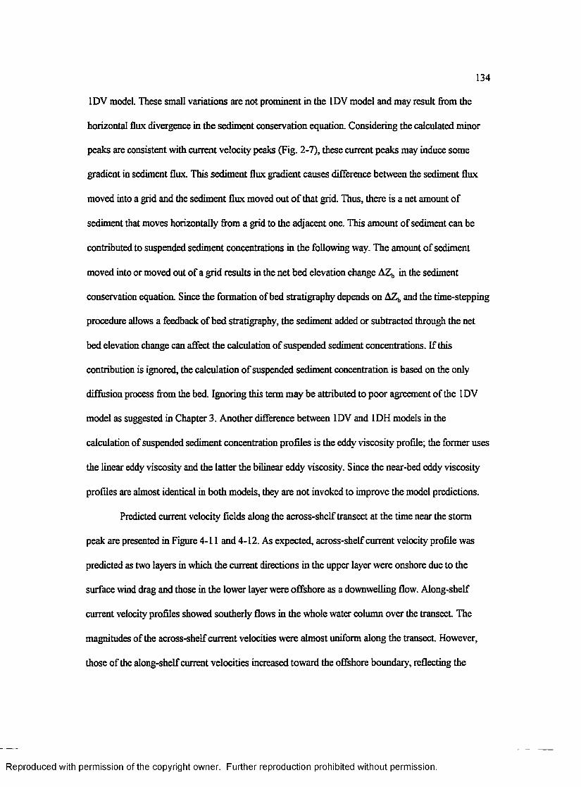
134

1DV model. These small variations are not prominent in the 1DV model and may result from the

horizontal flux divergence in the sediment conservation equation. Considering the calculated minor

peaks are consistent with current velocity peaks (Fig. 2-7), these current peaks may induce some

gradient in sediment flux This sediment flux gradient causes difference between the sediment flux

moved into a grid and the sediment flux moved out o f that grid. Thus, there is a net amount of

sediment that moves horizontally from a grid to the adjacent one. This amount of sediment can be

contributed to suspended sediment concentrations in the following way. The amount of sediment

moved into or moved out of a grid results in the net bed elevation change A i n the sediment

conservation equation. Since the formation of bed stratigraphy depends on A2^ and the time-stepping

procedure allows a feedback of bed stratigraphy, the sediment added or subtracted through the net

bed elevation change can affect the calculation of suspended sediment concentrations. If this

contribution is ignored, the calculation of suspended sediment concentration is based on the only

diffusion process from the bed. Ignoring this term may be attributed to poor agreement of the 1DV

model as suggested in Chapter 3. Another difference between 1DV and 1DH models in the

calculation of suspended sediment concentration profiles is the eddy viscosity profile; the former uses

the linear eddy viscosity and the latter the bilinear eddy viscosity. Since the near-bed eddy viscosity

profiles are almost identical in both models, they are not invoked to improve the model predictions.

Predicted current velocity fields along the across-shelf transect at the time near the storm

peak are presented in Figure 4-11 and 4-12. As expected, across-shelf current velocity profile was

predicted as two layers in which the current directions in the upper layer were onshore due to the

surface wind drag and those in the lower layer were offshore as a downwelling flow. Along-shelf

current velocity profiles showed southerly flows in the whole water column over the transect The

magnitudes of the across-shelf current velocities were almost uniform along the transect. However,

those of the along-shelf current velocities increased toward the offshore boundary, reflecting the


135

o

oooCO

ooinCMco

o © O O o ccm m

oinQ .

ooo

coo(ill) Midaa

Figure 4-11. Predicted current velocity fields along the transect showing across-shelf current velocity profiles at the time near the storm peak.


136

<DOOO

oo

o(D</)£o>

oCO

/ o /' 04/

O CO CO o COCN CO O

(iu) mdsa

Figure 4-12. Predicted current velocity fields along the transect showing along-shelf current velocity profiles at the time near the storm peak.


500

1000

15

00

2000

25

00

3000

35

00Di

stanc

e (m

)

Con

cent

ratio

n pr

ofile

(g/l)

; Ho

ur 8

,15

Oct

ober

137

coo ' / I /

too '

to

o CO CO o CO oo o

(uOiiidaa ”

Figure 4-13. Predicted concentration fields along the transect at the time near the storm peak.


500

1000

15

00

2000

25

00

3000

35

00Di

stanc

e (m

)

UC

(g/l)

(cm

/sec

); H

our

8, 15

Oct

ober

138

o I

ioo '

o CO CO o CO CO o

(ui) m d aa "

Figure 4-14. Predicted local sediment flux fields along the transect showing across-shelf local sediment flux profiles at the time near the storm peak.


500

1000

15

00

2000

25

00

3000

35

00Di

stanc

e (m

)

139

/ /

o

CO/ / /

O)

CO

o

o CO CO o CO 00 o

(uOmdaa "

Figure 4-15. Predicted local sediment flux fields along the transect showing along-shelf local sediment flux profiles at the time near the storm peak.


500

1000

15

00

2000

25

00

3000

35

00Di

stanc

e (m

)

140

frictional effect o f inner-shelf geometry.

Suspended sediment concentration fields along the transect are presented in Figure 4-13. The

contour lines of the various concentrations were distributed regularly as a sigmoidal shape. As a

result, they showed larger horizontal gradient than the current velocities and also showed more or less

increased vertical gradient at the water surface. This characteristic distribution of suspended

sediment concentration may be produced by the wave field. The intensity of wave orbital velocity

increases with decreasing depth and more sediment is resuspended. It results in larger horizontal

gradient of suspended sediment concentration.

Using two fields presented in above, we obtained local suspended sediment flux fields, mean

concentration multiplied by mean velocity at a certain elevation, along the transect (Fig. 4-14 and 4-

15). The distribution of across-shelf flux, UC, was similar to that o f the across-shelf current velocity.

The distribution of along-shelf flux, VC, was closer to the concentration field rather than that of the

along-shelf current velocity. It is noted that the local suspended sediment flux near the surface in

Figure 4-14 is not negligible.

Temporal and spatial variations of predicted shear velocities are presented in Figure 4-16

and 4-17. Bottom shear velocities due to wind-driven currents u.b varied predominantly with respect

to time but their spatial variation was negligible. Shear velocities due to the combined flows, u .^ ,

varied with time and space. Spatial gradient of u .^ was highly correlated to its spatial mean value

which was chosen as its representative value at a specified time (Fig. 4-18). This means that higher

wave energy is accompanied by larger spatial gradient of u>cw. High waves increase the magnitude as

well as the across-shelf gradient of suspended sediment concentration. So waves are very important

in determining flux divergence in the sediment conservation equation and eventually morphological

changes. Wind-driven currents must play an important role in determining not only the magnitude but

also the direction of sediment flux. However, the currents are not deterministic for the spatial


141

o(UWEo

-Q*3

1 I I I . ,

- SO -

_ _

inX—

CM

CM

IDO

-LOx—

-

inX—

“

------- 1----------------- 1------------- CM

00 CM CD

(uj) n;d8QCO o

CM

05

00

CD

ID

00

CM

CMCM

Figure 4-16. Contour map showing distribution of predicted shear velocities due to current with respect to space and time.


Days

fro

m 1

Oct

ober

, 19

94

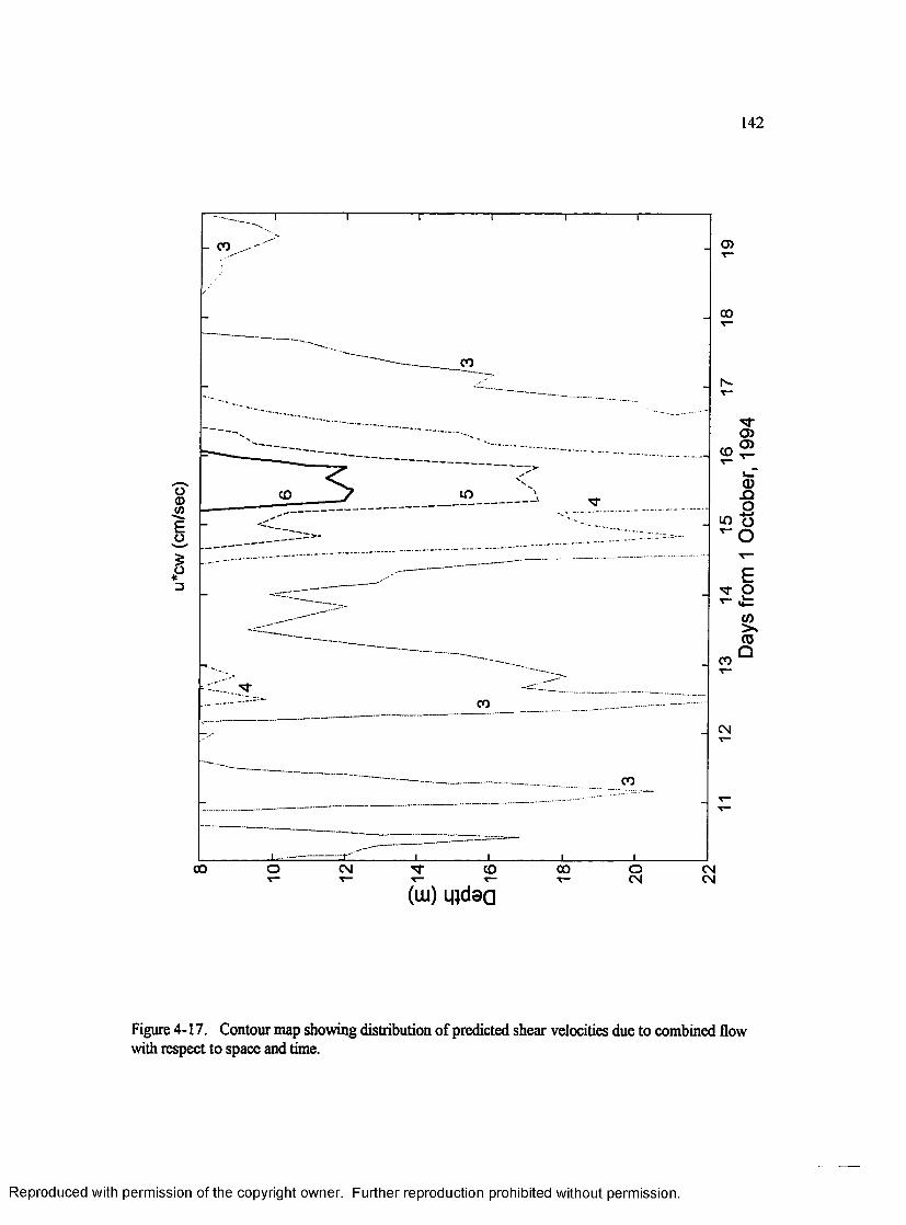
142

O)CO

CO

CO

od)COEo

10

CO

CO

CO

oCO C M CO oCO CMT- T - T - CM CM(ui) m daa

Figure 4-17. Contour map showing distribution of predicted shear velocities due to combined flow with respect to space and time.


Days

fro

m 1

Oct

ober

, 19

94

143

Corr. coef. = 0.9254

+f0.8

0.6

0.4-

0.23.52 2.5 3 4 4.5 5 5.5 6

u*cw

Figure 4-18. Correlation between predicted shear velocity due to combined flow, u .^ , and spatial gradient of .


144

gradient of sediment flux. As shown in Figure 4-19 and 4-20, the across-shelf and along-shelf

sediment fluxes were simultaneously related to both waves and currents. The distributional pattern of

sediment flux was not exclusively related to either waves or currents. Both magnitude and spatial

gradient of the sediment flux were maximum at the storm peak. To examine relationships between

the sediment flux and both waves and currents, the time series of sediment flux at the 20 m depth

was taken from the contour map (Fig. 4-21) and the time series of u.b and u.^, were made (Fig. 4-22).

Comparisons between both figures clearly demonstrated that synchronization of waves and currents

resulted in a higher sediment flux. Therefore, we can postulate that morphological changes on the

inner shelf during a high energy event occur with synchronized wave and current activities. In other

words, either wave or current events alone, for example, the wind peak at the onset of the storm, will

not give significant effect on sediment flux and then morphological changes.

Predicted direction of across-shelf sediment flux was dominantly offshore. Onshore

sediment transport occurred at the end of the storm (Fig. 4-21) when southerly winds caused

upwelling currents. But the peaks from 17 to 18 October were related to unstable behaviors o f the

Jenter and Madsen model which occur when the wind direction is nearly parallel to the coastline (see

Fig. 2-5).

The time series of bed elevation along the transect showed accretion of inner-shelf bed

during the storm period (Fig. 4-23). A rapid increase in the net bed elevation change occurred during

the storm peak and overall accretion of the bed elevation was about 2 mm (Fig. 4-24). The time

series representing the net bed elevation change A , which is similar to the time series representing

the sediment flux, present the erosion/deposition sequences during the storm period (Fig. 4-25).

Offshore sediment flux was directly related to deposition and onshore sediment flux to erosion.

Another feature was that the bed elevation change was greater in shallow water depths than deeper

water depths, implying that source of sediment was in shallow water depths, i.e., the surf zone. These


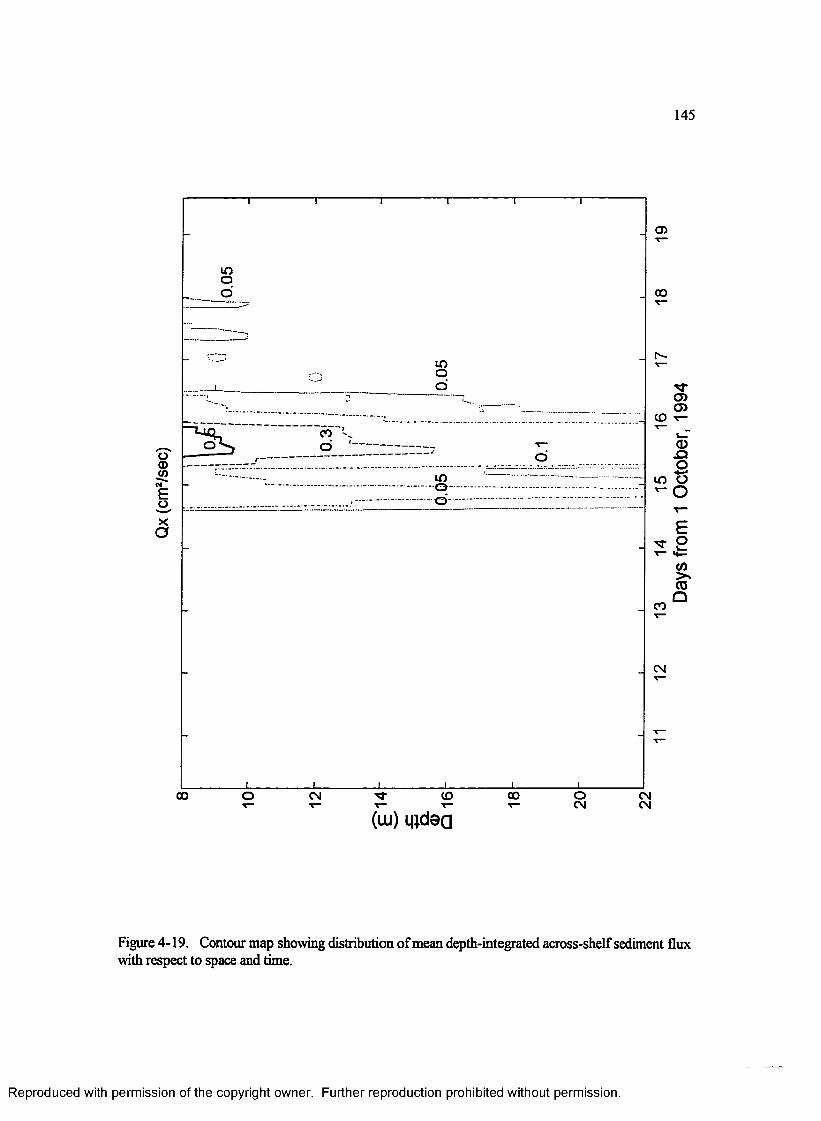
145

CD

mco

oCDm5"Eo

omG

OXa

CO

CM

OCM

O CD COCO CM CMCM

(w ) i |;d 0 Q

Figure 4-19. Contour map showing distribution of mean depth-integrated across-shelf sediment flux with respect to space and time.


Days

fro

m 1

Oct

ober

, 19

94

146

05

CO

COO

o0JO«Eo

in

>%a

co

CN

CO 00 oCO o

(UJ) if lc te a

Figure 4-20. Contour map showing distribution of mean depth-integrated along-shelf sediment flux with respect to space and time.


Days

fro

m 1

Oct

ober

, 19

94

147

(a) Flux at 20m0.2

0.15

0.1

0.05

-0.05

- 0.1(b)

5 T

-10

-1510 12 14 16 18 20


Figure 4-21. Time series of across-shelf (a) and along-shelf (b) sediment flux at 20 m depth.


148

2.5

0.8

0.60.5

0.4

0.216 18 2010 12 14


Figure 4-22. Time series of shear velocity due to current (solid line) and shear velocity due to combined flow (dashed line) at 20 m depth.


u cw

149

facts can be explained by the characteristic concentration field produced by the waves and the

direction of wind-driven currents. The horizontal gradient o f suspended sediment concentration can

be regarded as supporting two sources of sediment surplus and deficit, which are located at shallow

water and deep water depths, respectively. When the direction o f wind-driven currents is offshore

(downwelling), the higher concentration moves toward deep water, so the inner shelf acts as a sink of

sediment. On the contrary, the lower concentration (deficit) moves toward shallow water during

upwelling and consequently the inner shelf acts as a source of sediment. Therefore, both waves and

wind-driven currents are crucial to determining the erosion/deposition of bed elevation. The inner-

shelf bed responds dynamically to these variables during a high energy event.

Compared with field measurements (Fig. 2-11), the time series of near-bottom orbital

velocities appears to qualitatively agree with predicted u .^ values. The differences between wave

orbital velocities at the 12 m and 20 m depths were proportional to the intensity of the waves. Also,

current velocities at the two locations were generally close during the storm event except during the

storm peak when some difference existed. Another discrepancy was that current velocity was larger

at the onshore site than at the offshore site. These discrepancies between the model predictions and

the field measurements might come from non-wind-induced processes. Since currents play an

important role in determining sediment flux, we need to predict them with confidence. The predicted

currents were almost uniform with respect to space, so that they could have led to an underestimation

of sediment flux.

Field measurements o f bed elevation changes were quantitatively and qualitatively different

from the model predictions. The predicted bed elevation changes were about two orders of magnitude

smaller than the field measurements presented in Figure 2-11. Even if we include along-shelf

sediment flux that is an order of magnitude greater than across-shelf sediment flux, the model still

underestimates by about an order of magnitude. Currently, no resolution of this problem is


150

R e p ro d u c e d with

coT-ssojov

o

Figure 4 23 T**

Permission of the copyright owner. Further™™™. .reproduction prohibited without permission.

Z (c

m)

151

05

COCOo

o ,CN

O

CO

m

co

CN

co co CNCN

CO o CN

(uu) MJdaa

Figure 4-24. Contour map showing bed elevation changes with respect to space and time.


Days

fro

m 1

Oct

ober

, 19

94

152

(a)0.015

0.01

0.005

-0.005

- 0.01(b)

0.2 T T T T

12m

® 0.

16m

20m


Figure 4-25. Time series of the net change of bed elevations (a) and the cumulative elevations (b) at 12 m, 16 m, and 20 m depths.


153

immediately available. Qualitatively, the field measurements at the 12 m depth showed two

depositional phases concurrent with the current velocity peaks. However, the model predicted just

one depositional phase at the storm peak. Both model predictions and field measurements seemed to

agree in the last stage of the storm when the erosional phase occurred. It is worth noting that the bed

elevation changes at two locations were not in phase during the first depositional phase when erosion

occurred at the 20 m depth. The first depositional phase at the 12 m depth does not agree with the

model predictions and might have resulted from sinkage of the tetrapod. If this is the case,

approximately 15 cm of the change can be regarded as caused by the sink.

The distribution of bed stratigraphy along the across-shelf transect as expressed by the

predicted spatial variation of storm deposits is shown in Figure 4-26. The thickness of the storm

deposits as well as the vertical gradient o f sediment size was associated with depth. Both thickness of

storm deposits and the vertical gradient of sediment size increased toward shallow water. This

implied that the surface sediment in shallow water had the smallest grain size after the storm event

(Fig. 4-27). This can be explained by the analysis in Chapter 3 where the modeled erosion depth is

relevant to the segregation of sediment size in the sediment column, assuming a negligible flux

divergence. As expected, the vertical gradient of sediment size was related to the erosion depth

shown in Figure 4-28. The erosion depth was generally much larger than the bed elevation changes

induced by the sediment flux divergence. Sediment flux weakly influenced the sediment size

distribution. However, it is noted that sediment transport will be important to bed stratigraphy on a

long-term basis.


10m

12m

14m

16m

18m

20m

154

-

1“. _r . - .. (

i

"o -

1 I I l i

. o-

lOo 'I

ini ni

coi

(luo) aoepns eifl luojj. iiidaQ

Figure 4-26. Predicted bed stratigraphy along the across-shelf transect. Circle represents the median diameter of sediment layer.


12

34

56

1

23

45

6

12

34

56

1

23

45

6

12

34

56

1

23

45

6

Size

class

(p

hi)

155

ooco

co

Q .

oocviTJ C N

C O

C O

CO

C N

00 o ooCN OCN

CN

(UJ) iflctea

Figure 4-27. Contour map showing distribution of the median diameter of the top 1 cm thick bed with respect to space and time.


Days

fro

m 1

Oct

ober

, 19

94

Eros

ion

dept

h (c

m)

156

05O

Of

00

o

CMO

CM

O CO 00 oCO

(IU ) i i j d a a

Figure 4-28. Contour map showing distribution of the erosion depth with respect to space and time.


Days

fro

m 1

Oct

ober

, 19

94

5. CONCLUSIONS

Two process-based models for sediment transport and strata formation on the inner shelf

during a high energy event were developed in this study. One was the vertical one-dimensional model

(1DV model) which deals with the coupling of boundary layer processes with bed stratigraphy,

neglecting the flux divergence term. The Grant and Madsen (1986) model was implemented for the

hydrodynamics module. The armoring processes and the processes that cause changing sediment size

were solved explicitly using the simplified sediment conservation equation. One of the basic

assumptions was that the system reaches an equilibrium state in a time scale of hours and this was

used to close the problem.

The other model was the horizontal one-dimensional, depth-resolved model (1DH model)

which treats across-shelf sediment transport by including the horizontal flux term in the sediment

conservation equation. To estimate wave and current fields, a simple wave transformation model and

the Jenter and Madsen (1989) model were used. In the calculation of sediment flux, the bed

stratigraphy was coupled under the same assumptions as used in the 1DV model. Bed elevation

changes were solved explicitly by the backward difference scheme with an offshore boundary

condition of zero sediment transport.

The unique feature of the 1DV model was to defining the total depth of change as the sum of

the erosion depth and the mixing depth. This length scale was introduced to provide sediment

availability to the suspended sediment It supports a more rigorous treatment than the mixing depth

alone can. Another feature of this model was coupling of the bed stratigraphy using parameterized

157


158

bed inputs. Theoretically, the mixing depth, armoring process, and changing bottom sediment

processes are not independent but mutually dependent The problem is not closed if any one of these

processes is neglected. The following features must be included to incorporate the armoring process

in a composite model; (1) the variation of the grain size distribution in an armored layer, (2) the

variation of the armored layer thickness, (3) the independence of the armored bed from the suspended

sediment concentration, and (4) the bed stratigraphy as an output of the model. A feedback procedure

between the hydrodynamics and the bed stratigraphy was established.

The field measurements were performed in October 1994 as a part o f the CoOP’94

experiment off Duck, North Carolina. Wind, wave, current measurements made during an extra-

tropical storm were used for model inputs. A simplified bed stratigraphy provided sediment

parameters. Both models were adjusted using field measurements of the suspended sediment

concentration to determine the resuspension coefficient Yo- The adjusted models resulted in the

resuspension coefficient values y0 = 0.001 for the 1DV model and y0= 0.002 for the IDH model,

respectively. Suspended sediment concentrations predicted by the IDH model were closer to the field

observations than those predicted by the IDH model. This was attributed to the contribution of

horizontal sediment flux The Yo values were close to the Smith and McLean’s (1977) value. The

resuspension coefficient is assumed to remain constant over the time-varying flow conditions in order

to treat bed concentration as a variable. This makes it difficult to estimate the y0 values inversely

using field observations of suspended sediment concentration. The major features of the model

predictions are described in the following.

Coupling of boundary layer processes with bed stratigraphy was critical to improving

predictions of suspended sediment concentration. The decoupled model resulted in the resuspension

coefficient y0 = 3 x lO-4 which was close to the value suggested by Madsen et al. (1993). Good

agreement between model predictions and field measurements of suspended sediment concentration


159

was not achieved because the decoupled model overestimated suspended sediment concentration at

higher elevations and underestimated at lower elevations. However, in terms of ability to predict

hydrodynamic variables, the decoupled model was equivalent to the coupled model. Small changes in

the bottom sediment had little effect on the hydrodynamics but greatly affected sediment transport.

The bed was as important in controlling the sediment transport as the flow and both bed and flow

controls should be modeled simultaneously to predict sediment transport with confidence.

Predicted bed stratigraphy showed that the major influence of a resuspension event was to

increase the vertical gradient of the sediment size in a sediment column. Deeper erosion depths

resulted in larger vertical gradients of sediment size, forming the typical fining upward sequence of

storm deposits. This may explain the reduced bed micro-morphology immediately after a high energy

event. In this qualitative aspect, the behavior of the model was accurate. Thin surface layers of

bottom sediment appeared to show fining upward trends which may result from a storm event.

However, more rigorous comparisons require a long-term model and careful treatment o f sediment

size variations.

The IDH model showed the effects of wind-driven processes on across-shelf sediment

transport and inner-shelf morphology. Wind-driven currents, forming a more or less uniform current

field, were responsible for the magnitude as well as the direction of the sediment flux. A

characteristic sigmoidal shape of the concentration field was produced by the wave field, meaning

that waves were important to the horizontal gradient of the suspended sediment concentration.

Therefore, flux divergence depended on the waves. The coexistence of waves and currents was

responsible for large flux divergence and morphological changes. The results also showed that

shoreface deposition occurred during downwelling currents whereas erosion was associated with

upwelling currents. Thus, inner-shelf morphology responded dynamically to imposed wind-stresses

and waves as either a sink o f sediment or a source of sediment.


APPENDIX A

The Effects of Measurement Height Changes on the Velocity Profiles

In t r o d u c t io n

From mean velocity profiles measured in the benthic boundary layer, bed shear stress and

roughness can be calculated based on the assumption of the logarithmic 'law of the wall'. These

parameters are crucial to estimating quantities of sediment transport This technique is typically

performed using an instrumented tripod equipped with current meters vertically arranged at several

heights, recorders, and control systems [Grant and Madsen, 1986; Wright, 1989], Numerous

uncertainties in field instrumentation may cause the ideal logarithmic profile to be a curved line on a

log-linear plot. Sources of uncertainty generally are properties of real flows such as low-frequency

internal waves, stratification, and flow accelerations [Soulsby and Dyer, 1981; Grant et al., 1984;

Dyer, 1986] or measurement errors including inaccuracies o f a velocity sensors and uncertainty in the

distance from the velocity sensors to the seabed [Wiberg and Smith, 1983; Grant et al., 1984; Gross

etal., 1992],

Wiberg and Smith [1983] related a velocity profile with a concave-upward curvature to

instrument settlement. A zero-plane adjustment resulted in better prediction of the roughness

parameter [Wiberg and Smith, 1983; Grant et al., 1984], Their method was to choose the

displacement height that maximized the R2 values for all velocity profiles. This ignored the

possibility of time-varying displacement. The displacement height might be defined as a collective

160


161

term accounting for relative change in the measurement height due to both the vertical movement of

the instrument frame and the deposition/erosion of sediment Therefore, the time variant

displacement height was natural in this definition. Moreover the positive displacement might be

acceptable although Gross et al. [1992] argued that it is not physically reasonable in light of

instrument settling.

When a real velocity profile was assumed to be logarithmic, a simple equation having a

displacement height term, similar to Jackson's [1981], was found to represent the displaced velocity

profile. This equation was solved using the least square method and only velocity profile

measurements [Robinson, 1962; Steams, 1970]. One goal is to test the usefulness and examine the

nonlinear property of the equation.

Since the equation contains one more parameter to be determined compared to the

conventional velocity profile fitting method, it requires an independent technique to find one of the

three parameters [Soulsby and Dyer, 1981], An instrument such as the Digital Sonar Altimeter can

be deployed to keep tracks for the measurement height. In an alternate way, the shear velocity term

can be determined by the inertial dissipation method which requires the turbulent part of velocity

measurements [Huntley, 1988; Xu et al., 1994], However, it was not always easy to get highly-

qualified data for these methods. Therefore, it is desirable to seek a method to determine all

parameters without relying on an independent method.

Th eo retical A pproach

When the instrument moves an unknown distance vertically, the actual measurement heights

of velocity sensors become unknown. The heights of sensors will be different from the initially

measured ones on the hard surface before deployment All sensors experience the same amount of

change in the distance from sensors to seabed. In case that the distance is reduced, the sensors will


162

record lower values of velocity than what should be seen if the instrument is not moved. On the

contrary, the higher velocity will be measured when the instrument goes upward. This means that the

velocity measurements without accurate information about measurement heights will not give

realistic velocity profiles. Therefore, the departure from the logarithmic velocity profile can occur

because of the use of misleading measurement heights.

This simple relationship can be shown in the log-linear plot of a velocity profile (Fig. 1). The

straight line in Figure 1 represents an assumed logarithmic profile before the instrument is moved.

When the instrument is lowered in some distance, for example, 10 cm in Figure 1 the logarithmic

profile is changed to the concave-upward displaced profile in which the degree o f curvature (i.e., the

departure from the logarithmic profile) increases toward the bed. In a hypothetical upward

displacement of the instrument, the displaced profile becomes concave-downward. The form of

curvature is reversed compared with the profiles induced by accelerating flows [Soulsby and Dyer,

1981], As going away from the bed, the displaced profile approaches asymptotically to the

logarithmic velocity profile.

Derivation o f equation

When a velocity profile is logarithmic, we have

where U(z) is the mean velocity, u. is the shear velocity, k is the von Karman's constant, z is the

vertical elevation, and z0 is the roughness. This logarithmic velocity profile corresponds to the solid

straight line in the log-linear plot (Fig. 2). The straight line is changed to the broken curve when

measurement heights are lowered as much as a displacement height d. This displaced profile can be

expressed as equation (4) through a simple coordinate transformation. However, the following


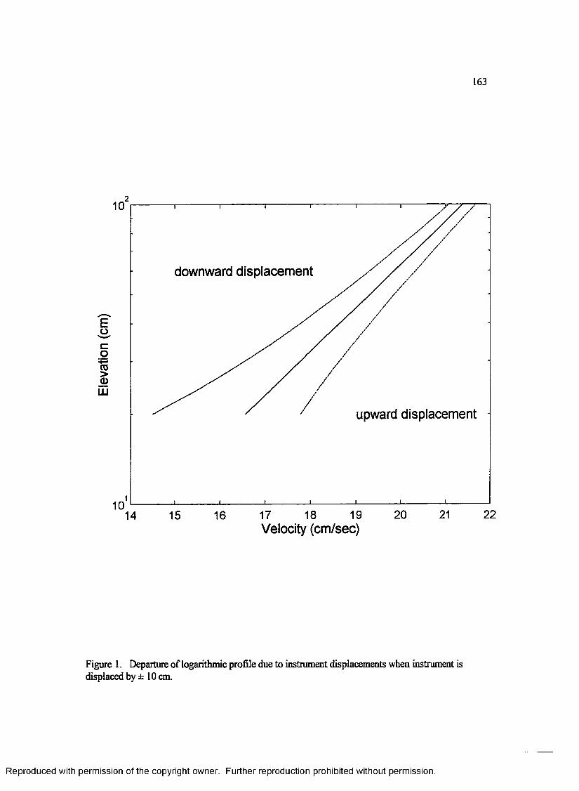
Elev

atio

n (c

m)

163

10

downward displacement/

upward displacement

1014 15 16 17 18 19 20 21

Velocity (cm/sec)22

Figure 1. Departure of logarithmic profile due to instrument displacements when instrument is displaced by ± 10 cm.


164

coCD>ffiUl

U(z)z-d

z+d

U UVelocity

Figure 2. Definition sketch showing the relationship between logarithmic profile and displaced profile.


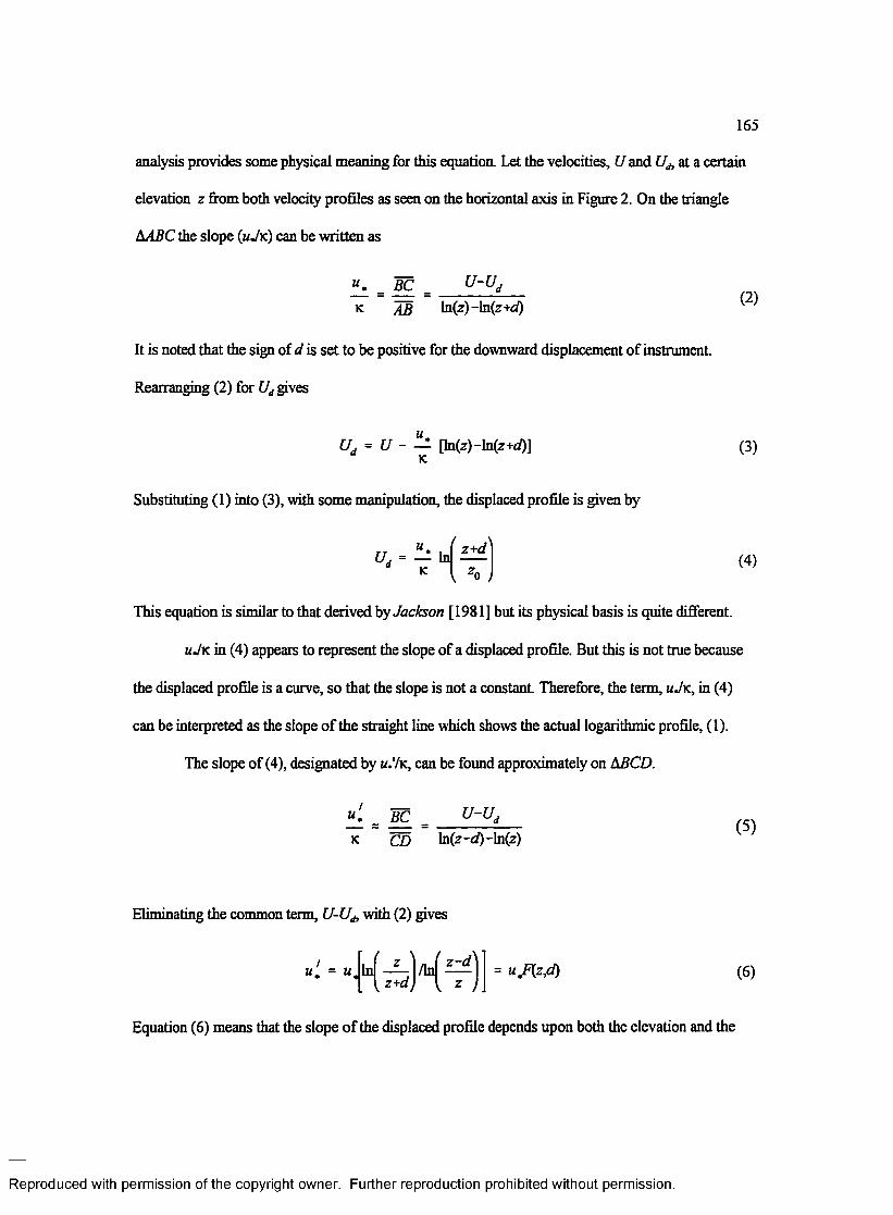
165

analysis provides some physical meaning for this equation. Let the velocities, U and U& at a certain

elevation z from both velocity profiles as seen on the horizontal axis in Figure 2. On the triangle

AABC the slope ( u J k ) can be written as

_ B C _ U~Ud k AB ln(z)-ln(z+eQ

It is noted that the sign of d is set to be positive for the downward displacement of instrument.

Rearranging (2) for Ud gives

(2)

U. = U - — [ln(z)-ln(z+<0]K

Substituting (1) into (3), with some manipulation, the displaced profile is given by

U; = — In z+dzn

(3)

(4)

This equation is similar to that derived by Jackson [1981] but its physical basis is quite different.

u J k in (4) appears to represent the slope of a displaced profile. But this is not true because

the displaced profile is a curve, so that the slope is not a constant Therefore, the term, u J k , in (4)

can be interpreted as the slope o f the straight line which shows the actual logarithmic profile, (1).

The slope of (4), designated by m. ' / k , can be found approximately on ABCD.

U-U;BCCD ln(z-<aO-ln(z)

(5)

Eliminating the common term, U-Uj, with (2) gives

u . = u. (6)

Equation (6) means that the slope of the displaced profile depends upon both the elevation and the


166

displacement height The vertical gradient of function F(z,d) is greater near the bed and decreases

asymptotically with increasing height

The intercept of (4), z0\ is given by zQ-d when U/z)= 0. Hence the term z0 in (4) does not

stand for the roughness parameter in the displaced profile. It is the roughness of the assumed

logarithmic velocity profile which is not displaced.

In summary, if the shear velocity and roughness parameters are taken from the equation (4)

as usual, they will contain properties of not the displaced profile but the actual logarithmic profile.

This simple relationship explored in this manner shows that additional terms are not necessary for

calculating the real shear stress and roughness parameters.

Least square method

The method to solve for three parameters, u., z0 and d is adopted with those described in

Robinson [1962] and Steams [1970], The observed variables, U and z, are treated as input variables,

denoted as a subscript i in the equation given by

£/*,. - U, ln|

t \zt+d

where 1 z i z M ( 7 )

in which M is the number of observations and u J k is substituted into U. for simplicity. Here z, is an

initially measured height of the ith velocity sensor rather than the actual observed data. A solution for

the three profile parameters is sought by the least square method which minimizes the sum of error

squares between the observed velocity data at several heights and the values calculated by the model

equation (7). Since the derivation of solution is identical to the previous work conducted by

Robinson [1962], many of the details will be skipped here.

M elements of an ordered array can be denoted by M dimensional components of a vector


167

and then the sum of the product between the elements of two arrays can be represented simply by the

scalar product of two vectors (a dot product). If we take a vector notation with regards to the

elements of a data array, the derivation to the solution will be simplified. So the error vector between

the observed data and calculated quantities with (7) is defined as

g = U*-Vcai = O-ujjc-W) (8)

where X=ln(z+d) and W=ln(z0). The sum o f error squares, therefore, is given by

e-e = [U -U £X-W )]iU -U m(X-W)] (9)

The condition to minimize (9) is that the partial derivatives of (9) with respect to U., d, and z0 are

zero, i.e.,

i l l = o — = 0 — = 0 (1 0 )dUm ’ dd ’ dzQ

Hence we have three equations from (10) that are given successively forz0, U., and d,

w - K = xm-u;lum (ii)

u , = (u-v)/(rx) (12)

fid) = (u-x)(x-b)-(x-x)(u-b) (13)

where Wm, ^ , Um, and Bm , denote the vector of mean in which all components are equal to its

mean, B is a vector substituted for dX/dd, and vectors subtracted by its mean, for example, U-Um, are

indicated by lowercase vectors u, x, and b.

An iteration technique may be applied to solve for (13) which is a function of the only


unknown d. The secant method is appropriate in practice because this numerical technique requires

no derivatives and converges at the efficient rate, the convergence order 1.62 [Robinson, 1962].

However, it needs the caution that two successive initial guesses (a bracket) should be properly set in

the small side from the maximum point of (13). The tolerance on d is good enough at 0.1 cm. After d

is determined, U. and z0 are solved in (12) and (11) by successive substitutions.


REFERENCES

Abramowitz, M. and I. A. Stegun, 1972. Handbook o f mathematical functions. National Bureau of Standards Applied Math Series, No. 55.

Bailard, J. A., 1981. An energetics total load sediment transport model for a plane sloping beach. J. Geophys. Res., 86,10,938-10,954.

Bathes, J. A., 1988. Surf-zone dynamics. Ann. Rev. FluidMech., 20,257-293.

Battjes, J. A., R. J. Sobey, and M. J. F. Stive, 1990. Near shore circulation, in The sea Vol. 9, Ocean Engineering Science, edited by LeMehaute, B. and D. M. Hanes, p.467-494. John Wiley, New York.

Bedford, K. W. and J. Lee, 1994. Near-bottom sediment response to combined wave-current conditions, Mobile Bay, Gulf of Mexico. J. Geophys. Res., 99, 16,161-16,177.

Birkemeier, W. A., H. C. Miller, S. D. Wilhelm, A. E. DeWall, and C. S. Gorbics, 1985. A user’s guide to the coastal engineering research center’s (CERC’s) field research facility. Instruction Report CERC-85-1, U. S. Army Corps of Engineers, Waterways Experiment Station, Vicksburg, Mississippi. 121 pp.

Borah, D. K., C. V. Alonso, and S. M. Prasad, 1982. Routing graded sediments in streams: formation. J. Hydraulic Eng., ASCE, 108, 1486-1503.

Chin, C. O., B. W. Melville, and A. J. Raudkivi, 1994. Streambed Armoring. J. Hydraulic Eng., ASCE, 120, 899-918.

Chisholm, T. A., 1993. Analysis of field data on near bottom turbulent flows and suspended sediment concentrations. C. E. Thesis, MIT.

Conley, D. C. and D. L. Inman, 1992. Field observations of the fluid-granular boundary layer under near-breaking waves. J. Geophys. Res., 97,9631-9643.

Data Announcement 88-MGG-02, Digital relief of the surface of the Earth. NOAA, National Geophysical Data Center, Boulder, Colorado, 1988.

Data Announcement 95-MGG-02, GEODAS CD-ROM DATA SET Version 3.1. NOAA, National Geophysical Data Center, Boulder, Colorado, 1995.

169


170

De Vriend, H. J., J. Zyserman, J. Nicholson, J. A. Roelvink, P. Pechon and H. N. Southgate, 1993. Medium-term 2DH coastal area modelling. Coast. Eng., 21,193-224.

Dean, R. G., 1991. Equilibrium beach profiles: Characteristics and applications. J. Coastal Res., 1, 53-84.

Dean, R. G. and R. A. Dalxymple, 1992. Water wave mechanics fo r engineers and scientists. Advanced series on ocean engineering, Vol. 2, World Scientific.

Drake, D. E. and D. A. Cacchione, 1989. Estimates of the suspended sediment referenceconcentration (CJ and resuspension coefficient (y0) from near-bottom observations on the California shelf. Cont. Shelf Res., 9,51-94.

Dyer, K. R., 1986. Coastal and estuarine sediment dynamics. John Wiley & Sons.

Folk, R. L., 1968. Petrology of sedimentary rock. HemphelTs, Texas.

Fredsoe, J. and R. Deigaard, 1993. Mechanics o f coastal sediment transport. Advanced series on ocean engineering, Vol. 3, World Scientific.

Gaughan, M. K., 1978. Depth of disturbance of sand in surf zone. Proceedings 16th International Conference Coastal Engineering, 1513-1530.

Gessler, J., 1970. Self-stabilizing tendencies of alluvial channels. J. Waterways and Harbors Division, ASCE, 96, WW2, Proc. Paper 7263,235-249.

Glenn, S. and W. D. Grant, 1987. A suspended sediment stratification correction for combined wave and current flows. J. Geophys. Res., 92, 8244-8264.

Grant, J., 1983. The relative magnitude of biological and physical sediment reworking in an intertidal community. J. Mar. Res., 41, 673-689.

Grant, W. D. and 0 . S. Madsen, 1979. Combined wave and current interaction with a rough bottom.J. Geophys. Res., 84,1797-1808.

Grant, W. D. and O. S. Madsen, 1982. Movable bed roughness in unsteady oscillatory flow. J. Geophys. Res., 87,469-481.

Grant, W. D. and O. S. Madsen, 1986. The continental-shelf bottom boundary layer. Ann. Rev. Fluid Mech., 18,265-305.

Grant, W. D., A. J. William, and S. M. Glenn, 1984. Bottom stress estimates and their prediction on the northern California continental shelf during CODE 1: The importance of wave-current interactions, J. Phys. Ocean., 14,506-527.

Green, M. O. and J. D. Boon, 1993. The measurement of constituent concentrations innonhomogeneous sediment suspension using optical backscatter sensors. Mar. Geol., 110, 73-81.


171

Gross, T. M., A. E. Isley, and C. R. Sherwood, 1992. Estimation of stress and bed roughness during storms on the northern California shelf, Cont. Shelf Res., 12,389-413.

Harris, C. K., 1994. Modeling long term continental shelf sedimentation: Sensitivity to fairweather processes, storm forcing fiinctions, and storm sequences. Master Thesis, Univ. of Virginia.

Hildebrand, F. B., 1976. Advanced calculus fo r applications, 2nd ed. Prentice-HalL

Hill, P. S., A. R. M. Nowell, and P. A. Jumars, 1988. Flume evaluation of the relationship between suspended sediment concentration and excess boundary stress. J. Geophys. Res., 93, 12,499- 12,509.

Holly, F. M. and Karim, M. F., 1986. Simulation of Missouri River bed degradation. J. Hydraulic Eng., ASCE, 112,497-517.

Hunt, J. N., 1979. Direct solution of wave dispersion equation, J. Waterways, Ports, Coastal Ocean Div., ASCE, 105, No. WW4,457-459.

Huntley, D. A., 1988. A modified inertial dissipation method for estimating seabed stresses at low Reynolds numbers, with application to wave/current boundary layer measurements, J. Phys. Ocean., 18,339-346.

Jackson, P. S., 1981. On the displacement height in the logarithmic velocity profile, J. FluidMech., I l l , 15-25.

Jenter, H. L. and 0 . S. Madsen, 1989. Bottom stress in wind-driven depth-averaged coastal flows. J. Phys. Ocean., 19,962-974.

Jonsson, I. G., 1966. Wave boundary layers. Proceedings 10th International Conference Coastal Engineering, Tokyo, 127-148.

Kachel, N. B. and J. D. Smith, 1986. Geological impact of sediment transporting events on theWashington continental shelf In: Knighf R. I. and McLean, J. R., (editors), Shelf Sands and Sandstones. Canadian Society o f Petroleum Geologists, Memoir H, 145-162.

Kache!, N. B. and J. D. Smith, 1989. Sediment transport and deposition on the Washingtoncontinental shelf In: Landry ,M. R. and Hickey, B. M., (editors), Coastal Oceanography o f Washington and Oregon. Amsterdam: Elsevier, 287-348.

Keen, T. R. and S. M. Glenn, 1994. A coupled hydrodynamic-bottom boundary layer model of Ekman flow on stratified continental shelves. J. Phys. Ocean., 24,1732-1749.

Kim, S. C., 1991. Inner continental shelf benthic boundary layer dynamics and suspended sediment transport. Ph. D. Thesis, The College of William and Mary, pp. 159.

Kim, S. C., L. D. Wright, and B. 0 . Kim, 1996. The combined effects of synoptic and local-scale meteorological events on bed stress and sediment transport on the inner shelf of the Middle


172

Atlantic Bight submitted

King, C. M. A., 1951. Depth of disturbance of sand on sea beaches by waves. J. Sedimentary Petrology, 21,131-140.

Kraus, N. C., 1985. Field experiments on vertical mixing of sand in the surf zone. J. Sedimentary Petrology, 55,3-14.

Kuhnle, R. A., 1989. Bed-surface size changes in gravel-bed channel. J. Hydraulic Eng., ASCE,115,731-743.

Lee, H.-Y. and A. J. Odgaard 1986. Simulation of bed armoring in alluvial channels. J. Hydraulic Eng., ASCE, 112,794-801.

Li, M. Z., L. D. Wright and C. L. Amos, 1996. Predicting ripple roughness and sand resuspension under combined flows in a shoreface environment Mar. Geoi, 130, 139-161.

Little, W. C. and P. G. Mayer, 1976. Stability o f channel beds by armoring. J. Hydraulic Division, ASCE, 102,1647-1661.

Liu, P. L.-F. and T.-K. Tsay, 1985. Numerical prediction of wave transformation. J. Waterway, Port, Coastal, Ocean Eng., ASCE, 111, 843-855.

Longuet-Higgins, M. S. and R. W. Stewart, 1964. Radiation stresses in water waves: a physical discussion, with applications. Deep Sea Research, 11,529-562.

Lu, J. -Y. and Shen, H. W., 1986. Analysis and comparisons of degradation models. J. Hydratdic Eng., ASCE, 112,281-299.

Ludwig, K. A. and D. M. Hanes, 1990. A laboratory evaluation o f optical backscatterance suspended solids sensors exposed to sand-mud mixtures. Mar. Geol., 94,173-179.

Lyne, V. D., B. Butnam, and W. D. Grant, 1990. Sediment movement along the U.S. east coastcontinental shelf-11. Modeling suspended sediment concentrations and transport rates during storms. Cont. Shelf Res., 10,429-460.

Maa, J. P.-Y. and S.-C. Kim, 1992. Effects of bottom friction on wave breaking using RCPWAVE model. J. Waterway, Port, Coastal, Ocean, Eng., ASCE, 118,387-400.

Madsen, O. S., 1974. Stability of a sand bed under breaking waves. Proceedings 14th International Conference Coastal Engineering, ASCE, Kobe, 776-794.

Madsen, O. S., 1977. A realistic model of the wind-induced Ekman boundary layer. J. Phys. Ocean., 7 ,248-255.

Madsen, O. S., 1991. Mechanics of cohesionless sediment transport in coastal waters. Coastal Sediment '91 Proceedings Specialty Conference, ASCE, 15-27.


173

Madsen, 0. S., 1994. Spectral wave-current bottom boundary layer flows. Proceedings 24th International Conference Coastal Engineering, ASCE, Kobe, 384-398.

Madsen, 0 . S., T. A. Chisholm, and L. D. Wright, 1994. Suspended sediment transport in inner shelf waters during extreme storms. Proceedings 24th International Conference Coastal Engineering, ASCE, Kobe, 1849-1864.

Middleton, G. V. and J. B. Southard, 1984. Mechanics o f sediment movement. 2nd ed. SEPM Short Course No.3.

Mitchum, G. T. and A. J. Clark, 1986. The frictional nearshore response to forcing by synoptic scale winds. J. Phys. Ocean., 6, 934-946.

Myers, A. C., 1977. Sediment processing in a marine subtidal sandy bottom community: I. Physical aspects. J. Mar. Res., 35, 609-632.

Nielsen, P., 1981. Dynamics and geometry of wave generated ripples. J. Geophys. Res., 86, 6467- 6472.

Nielsen, P., 1993. Coastal bottom boundary layers and sediment transport. Advanced series on ocean engineering, Vol. 4, World Scientific.

Niederoda, A. W., D. J. P. Swift, A. G. Figueiredo and G. L Freeland, 1985. Barrier island evolution, middle Atlantic shelf, U.S.A. part A: evidence from the shelf floor. Mar.Geol., 63,363-396.

Niederoda, A. W., D. J. P. Swift and J. A. Thome, 1989. Modeling shelf storm beds: controls of bed thickness and bedding sequence. Proceedings GCSSEPMFoundation Seventh Annual Research Conference, 15-18.

Nittrouer, C. A. and R. W. Sternberg, 1981. The formation of sedimentary strata in an allochthonous shelf environment: the Washington continental shelf. Mar. Geol., 42, 201-232.

Nittrouer C. A. and L. D. Wright, 1994. Transport of particles across continental shelves. Reviews o f Geophysics, 32, 85-113.

Park, I. and S. C. Jain, 1987. Numerical simulation o f degradation of alluvial channel beds. J. Hydraulic Eng., ASCE, 113, 845-859.

Parker, G. and P. C. Klingeman, 1982. On why gravel bed streams are paved. Water Resources Res., 18, 1409-1423.

Parker G., P. C. Klingeman, and D. G. McLean, 1982. Bedload and size distribution in paved gravel- bed streams. J. Hydraulic Eng., ASCE, 108, 544-571.

Pilkey, O. H., R. S. Young, S. R. Stanley, A. W. Sam Smith, H. Wu, and W. D. Pilkey, 1993. The concept o f shoreface profile o f equilibrium: a critical review. J. Coastal Res., 9 ,255-278.

Poon, Y. -K and O. S. Madsen, 1991. A two-layer wind-driven coastal circulation model. J.


174

Geophys. Res., 96,2535-2548.

Rahuel, J. L., F. M. Holly, J. P. Chollet, P. J. Belleudy, and G. Yang, 1989. Modeling of riverbed evolution for bedload sediment mixtures. J. Hydraulic Eng., ASCE, 115, 1521-1542.

Robinson, S. M., 1962. Computing wind profile parameters, J. Atmos. Se t, 19, 189-190.

Roelvink, J. A. and L Broker, 1993. Cross-shore profile models. Coast. Eng., 21,163-191.

Shi, N. C., L. H. Larsen, and J. P. Downing, 1985. Predicting suspended sediment concentration on continental shelves. Mar. Geol., 62,255-275.

Sanford, L. P. and J. P. Halka, 1993. Assessing the paradigm of mutually exclusive erosion and deposition of mud, with examples from upper Chesapeake Bay. Mar. Geol., 114, 37-57.

Sherman, D. J., K. F. Nordstrom, N. L. Jackson, and J. R. Allen, 1994. Sediment mixing-depths on a low-energy reflective beach. J. Coastal Res., 10,297-305.

Signell, R. P., R. C. Beardsley, H. C. Graber, and A. Capotondi, 1990. Effects of wave-currentinteraction on wind-driven circulation in narrow, shallow embayments. J. Geophys. Res., 95, 9671-9678.

Sleath, J. F. A., 1978. Measurements of bedload in oscillatory flow. J. Waterway Port Coastal Ocean Div., ASCE, 104,291-307.

Smith, J. D. and S. R. McLean, 1977. Spatially averaged flow over a wavy surface. J. Geophys. Res., 82,1735-1746.

Soulsby, R. L. and K. R. Dyer, 1981. The form of the near-bed velocity profile in a tidally accelerating flow, J. Geophys. Res., 86, 8067-8074.

Steams, C. R., 1970. Determining surface roughness and displacement height, Boundary-Layer Meteol., 1, 102-111.

Sunamura, T. and N. C. Kraus, 1985. Prediction of average mixing depth of sediment in the surf zone. Mar. Geol., 62, 1-12.

Swart, D. H., 1974. Offshore sediment transport and equilibrium beach profile. Delft Hydr Lab Publ No. 131.

Swift, D. J. P., A. W. Niederoda, C. E. Vincent, and T. A. Hopkins, 1985. Barrier island evolution, middle Atlantic shelf, U.S.A. part I: shoreface dynamics. Mar. Geol., 63,331-361.

Tan, W. -Y., 1992. Shallow water hydrodynamics. Elsevier Oceanography Series, 55, Water &Power Press.

Tanaka, H., 1988. Bed load transport of sediment with non-uniform grain size due to wave action. Coastal Engineering in Japan, 31,265-276.


175

Tiedeman, P. L., 1995. The effects of underlying geology on the equilibrium profile: a case study off Duck, North Carolina. M. Thesis, The College of William and Mary.

van Niekerk, A., K. R. Vogel, R_ L. Slingerland, and J. S. Bridge, 1992. Routing of heterogeneous sediments over moveable bed: Model development J. Hydraulic Eng., ASCE, 118,246- 262.

Vincent, C. E., D. M. Hanes, and A. J. Bowen, 1991. Acoustic measurements of suspended sand on the shoreface and the control of concentration by bed roughness. Mar. Geol., 96,1-18.

Vincent, C. E. and M. O. Green, 1990. Field measurements of the suspended sand concentration profiles and fluxes and of the resuspension coefficient y0 over a rippled bed. J. Geophys. Res., 95,11591-11610.

Wiberg, P. and J. D. Smith, 1983. A comparison of field data and theoretical models for wave- current interactions at the bed on the continental shelf. Cont. Shelf Res., 2, 147-162.

Wiberg, P. L., D. E. Drake, and D. A. Cacchione, 1994. Sediment resuspension and bed armoring during high bottom stress events on the northern California inner continental shelf: measurements and predictions. Cont. Shelf. Res., 14,1191-1219.

Wiberg, P. L. and C. K. Harris, 1994. Ripple geometry in wave-dominated environments. J.Geophys. Res., 99,775-789.

Wilcock, P. R. and J. B. Southard, 1988. Experimental study of incipient motion in mixed-size sediment Water Resources Res., 24,1137-1151.

Wilcock, P. R. and J. B. Southard, 1989. Bed load transport of mixed size sediment; Fractional transport rates, bed forms, and the development of a coarse bed surface layer. Water Resources Res., 25, 1629-1641.

Wilcock, P. R. and B. W. McArdell, 1993. Surface-based fractional transport rates: mobilizationthresholds and partial transport of a sand-gravel sediment. Water Resources Res., 29,1297- 1312.

Williams, A. T., 1971. An analysis of some factors involved in the depth of disturbance of beach sand by waves. Mar. Geol., 11,145-158.

Wilson, K. C., 1989. Friction o f wave-induced sheet flow. Coat. Eng., 12,371-379.

Wright, L. D., J. D. Boon, m, M. O. Green, and J. H. List, 1986. Response of the mid shoreface of the southern Mid-Atlantic Bight to a “Northeaster”. Geo-Marine Letters, 6, 153-160.

Wright, L. D., 1989. Benthic boundary layers of estuarine and coastal environments. Reviews in Aquatic Sciences, 1,75-95.

Wright, L. D., J. D. Boon, S. C. Kim, and J. H. List, 1991. Modes o f cross-shore sediment transport on the shoreface of the Middle Atlantic Bight. Mar. Geol., 96,19-51.


176

Wright, L. D., 1993. Micromorphodynamics of the inner continental shelf: A Middle Atlantic Bight case study. J. Coastal Res., 15, 93-124.

Wright, L. D., 1995. Morphodynamics o f inner continental shelves. Marine Science Series, CRC Press.

Wu, J., 1980. Wind-stress coefficients over sea surface near neutral conditions: a revisit. J. Phys. Ocean., 10,727-740.

Xu, J. P., 1993. Suspended sediment concentration profiles in the bottom boundary layer. Ph. D. Thesis, The College of William and Mary, pp. 131.

Xu, J. P., L. D. Wright, and J. D. Boon, 1994. Estimation of bottom stress and roughness in lower Chesapeake Bay by the inertial dissipation method, J. Coastal Res., 10, 329-338, 1994.

Xu, J. P. and L. D. Wright, 1995. Tests of bed roughness models using field data from the Middle Atlantic Bight Cont. Shelf Res., 15, 1409-1434.


VITAE

Baeck Oon Kim

Bom in Kimje, Korea, on February 3, 1965. Graduated from Kyungdong High School in

Seoul, Korea, in 1983. Earned B.S. in 1987 and M.S. in 1989 from the Department of Oceanography

of the Seoul National University in Korea. Served military service as an officers’ candidate of Korean

army in Yungcheon, Korea, in 1990. Entered the Ph.D. program in the Virginia Institute of Marine

Science, the College of William and Mary in 1991.

177

Documents

Modeling storm-induced sediment transport on the inner