Embed Size (px)
Citation preview

Brigham Young University Brigham Young University
BYU ScholarsArchive BYU ScholarsArchive
Theses and Dissertations
2011-12-13
Modeling Solid Propellant Ignition Events Modeling Solid Propellant Ignition Events
Daniel A. Smyth Brigham Young University - Provo
Follow this and additional works at: https://scholarsarchive.byu.edu/etd
Part of the Chemical Engineering Commons
BYU ScholarsArchive Citation BYU ScholarsArchive Citation Smyth, Daniel A., "Modeling Solid Propellant Ignition Events" (2011). Theses and Dissertations. 3125. https://scholarsarchive.byu.edu/etd/3125
This Dissertation is brought to you for free and open access by BYU ScholarsArchive. It has been accepted for inclusion in Theses and Dissertations by an authorized administrator of BYU ScholarsArchive. For more information, please contact [email protected], [email protected].

MODELING SOLID PROPELLANT IGNITION EVENTS
Daniel Austin Smyth
A dissertation submitted to the faculty of Brigham Young University
in partial fulfillment of the requirements for the degree of
Doctor of Philosophy
David O. Lignell, Chair Merril W. Beckstead Thomas H. Fletcher
Larry L. Baxter William C. Hecker
William G. Pitt
Department of Chemical Engineering
Brigham Young University
December 2011
Copyright © 2011 Daniel Austin Smyth
All Rights Reserved


ABSTRACT
Modeling Solid Propellant Ignition Events
Daniel Austin Smyth Department of Chemical Engineering, BYU
Doctor of Philosophy
This dissertation documents the building of computational propellant/ingredient models toward predicting AP/HTPB/Al cookoff events. Two computer codes were used to complete this work; a steady-state code and a transient ignition code. Numerous levels of verification resulted in a robust set of codes to which several propellant/ingredient models were applied. To validate the final cookoff predictions, several levels of validation were completed, including the comparison of model predictions to experimental data for: AP steady-state combustion, fine-AP/HTPB steady-state combustion, AP laser ignition, fine-AP/HTPB laser ignition, AP/HTPB/Al ignition, and AP/HTPB/Al cookoff. A previous AP steady-state model was updated, and then a new AP steady-state model was developed, to predict steady-state combustion. Burning rate, temperature sensitivity, surface temperature, melt-layer thickness, surface species at low pressure and high initial temperature, final flame temperature, final species fractions, and laser-augmented burning rate were all predicted accurately by the new model. AP ignition predictions gave accurate times to ignition for the limited experimental data available. A previous fine-AP/HTPB steady-state model was improved to predict a melt layer consistent with observation and avoid numerical divergence in the ignition code. The current fine-AP/HTPB model predicts burning rate, surface temperature, final flame temperature, and final species fractions for several different propellant formulations with decent success. Results indicate that the modeled condensed-phase decomposition should be exothermic, instead of endothermic, as currently formulated. Changing the model in this way would allow for accurate predictions of temperature sensitivity, laser-augmented burning rate, and surface temperature trends. AP/HTPB ignition predictions bounded the data across a wide range of heat fluxes. The AP/HTPB/Al model was based upon the kinetics of the AP/HTPB model, with the inclusion of aluminum being inert in both the solid and gas phases. AP/HTPB/Al ignition predictions bound the data for all but one source. AP/HTPB/Al cookoff predictions were accurate when compared to the limited data, being slightly low (shorter time) in general. Comparisons of AP/HTPB/Al ignition and cookoff data showed that the experimental data might be igniting earlier than expected. Keywords: Daniel Austin Smyth, solid propellant, model, steady state, combustion, ammonium perchlorate, AP, hydroxy-terminated poly-butadiene, HTPB, aluminum, ignition, cookoff


ACKNOWLEDGMENTS
It’s difficult to look back on such a long period of time and try to remember just how
many influences I’ve had during this time of my life. Major players will be easy to recall, while
others will likely be forgotten. It took me a long time to finally decide to even write this page
(it’s optional after all) because I didn’t want to forget anyone that had helped me. In the end, I’ve
decided that this is literally an impossible task. Still, I’m going to try my best at getting
everyone and everything down here. I’ll more than likely fail, but I guess it’s the attempt that
counts.
First, I think I need to thank my adviser and teacher during these last nine years: Dr.
Merrill Beckstead. I have no idea why he decided to even take me on as a graduate student in the
first place. Maybe he didn’t have a choice. I’m sure there have been times along the way that
he’s wished he hadn’t been given that last graduate student; that he’d been able to finish his
illustrious career on the high note of my predecessors and not have to deal with the frustration of
the kid that just wouldn’t take anything for granted. I’ve learned a lot from him and always tried
to take everything that I could from what he taught and apply it in a way that made sense to me.
I know our conclusions didn’t always agree. I guess that’s part of science though: looking at
everything we can and then making a determination from what we’ve seen. Regardless of the
outcome, I know that I’d never have been able to stand a chance at accomplishing the things I
did during this period of research without the knowledge and understanding that came from him
on a regular basis.
Second I need to thank my current adviser on this end of things, Dr. David Lignell. I
don’t think it’s too far of a long shot to say that I wouldn’t have been able to finish my research
had it not been for him. After Dr. Beckstead’s retirement, Dr. Lignell got up and swung for me


when it seemed like no one else wanted to. He’s not only given me the chance to finish the job I
set out to do, but helped to widen my view of combustion and simulation modeling as a whole.
Third goes to Dr. Tom Fletcher. He’s the one that helped me to even earn the right to be
accepted to graduate school. He helped me to find a way to do what I wanted to do: to learn
enough that I could be a go-to person when asking difficult technical questions. The lessons that
I’ve leared during graduate school have made that possible. I wouldn’t have even been able to
get my foot in the door without him.
Fourth, though first in matters pertaining to the heart, I need to thank my wife and the
unending support that she’s given me. Long hours away and longer nights alone have seemed to
be the norm for us, not only during these years of graduate school, but also during my
undergraduate years when I was trying to learn everything I could in the time that I had available
to me. I can never thank her enough for her patience and love and understanding; for her support
of me and the goals and dreams that I had during this time. I will forever be grateful to her and
to my three kids—Kaylee, Parker and Brenna—that prayed continually for my safety, health, and
success. It’s literally impossible to get too far down on life and its hardships when you have
such a wonderful family to come home to every night.
I’m thankful for my office mates and fellow partners in “research” crime: Karl Meredith,
Ephraim Washburn, Scott Felt, Matt Gross, Matt Tanner, Karthik Pudduppakkam, Mike
Hawkins, Johnathan Wierschke, Liz Monson, Derek Harris, and Guangyuan Sun. Countless
hours of brainstorming and trouble-shooting and debugging were spent in their company. Many
ah-ha moments and critical developments came as a result of their friendship. Jed Campbell
passed along a critical piece of advice to me (several times over several years) concerning


Designs of Experiment, and I can’t thank him enough for continuing to bother me until I gave in
and just did it. That’s a lesson that I won’t soon forget.
Many others provided non-technical and moral support during the tough times. My
parents and other family members played a very important role in keeping my spirits high.
Friends from my community and those from church. Friends from home, like Jeremy Brown,
who was always there to share and brighten my day and help me remember who I was. My
thanks go to all of them, but most importantly to Laren Robison, who never gave up on me and
was, even until the week before he passed away, telling me to keep fighting because I was going
to make it. The most difficult thing I ever did in graduate school was not quit, and it was people
like Laren that helped me make it all the way here.
Lastly I need to thank my Heavenly Father and his son, Jesus Christ, for making me the
person that I am—for teaching me and guiding me down life’s path in such a way that I could
learn those things that make me me. The strength and perspective that I’ve gained from keeping
them within my world-view has made everything worthwhile.

xi
TABLE OF CONTENTS LIST OF FIGURES .........................................................................................................................xv LIST OF TABLES ........................................................................................................................ xix NOMENCLATURE ...................................................................................................................... xxi
CHAPTER 1: INTRODUCTION ......................................................................................................1
CHAPTER 2: HISTORICAL PERSPECTIVE ..................................................................................7
2.1 STEADY-STATE PROPELLANT/INGREDIENT MODELING ..................................................7
2.1.1 AMMONIUM PERCHLORATE ........................................................................................12
2.1.1.1 LOW-TEMPERATURE DECOMPOSITION ..............................................................13 2.1.1.2 STEADY-STATE WORK .......................................................................................14
2.1.2 AP/HTPB .................................................................................................................21
2.2 IGNITION ..........................................................................................................................29
2.2.1 MODELING AND EXPERIMENTAL WORK .......................................................................31 2.2.2 MEREDITH IGNITION MODEL .....................................................................................35
2.3 COOKOFF ........................................................................................................................39
2.3.1 SLOW COOKOFF .........................................................................................................40 2.3.2 FAST COOKOFF..........................................................................................................41
CHAPTER 3: OBJECTIVES .........................................................................................................47
CHAPTER 4: CODE AND MODEL IMPROVEMENTS ...............................................................51

xii
4.1 PHASE3 CODE IMPROVEMENTS .....................................................................................51 4.2 IGNITION CODE IMPROVEMENTS ...................................................................................53 4.3 IMPROVEMENT OF THE STEADY-STATE AP MODEL .....................................................63
4.3.1 PART 1: UPDATING AND OPTIMIZING THE GROSS MODEL ............................................64 4.3.2 PART 2: RETHINKING THE AP MODEL .......................................................................72
4.3.3 SUMMARY ..................................................................................................................89
4.4 IMPROVEMENT OF THE STEADY-STATE AP/HTPB MODEL ..........................................90
4.4.1 AP/HTPB MODEL: 75% AP, 25% HTPB .................................................................98 4.4.2 AP/HTPB MODEL: 80% AP, 20% HTPB ...............................................................104 4.4.3 AP/HTPB MODEL: 84% AP, 16% HTPB ...............................................................106
4.4.4 SUMMARY ................................................................................................................108
4.5 HMX IGNITION .............................................................................................................110 4.6 SUMMARY OF FOUNDATIONAL WORK .........................................................................110
CHAPTER 5: IGNITION .............................................................................................................113
5.1 AP IGNITION .................................................................................................................114
5.1.1 RESULTS AND DISCUSSION ........................................................................................116 5.1.2 FURTHER ATTEMPTS TO VALIDATE THE STEADY-STATE MODEL ...................................129
5.1.3 SUMMARY ................................................................................................................133
5.2 AP/HTPB IGNITION .....................................................................................................134
5.2.1 RESULTS AND DISCUSSION .......................................................................................136
5.2.2 SUMMARY ................................................................................................................143 5.3 AP/HTPB/AL IGNITION AND COOKOFF ......................................................................144
5.3.1 IGNITION RESULTS AND DISCUSSION ........................................................................146

xiii
5.3.2 COOKOFF RESULTS AND DISCUSSION .......................................................................153
5.3.3 SUMMARY ................................................................................................................161
CHAPTER 6: SUMMARY AND CONCLUSIONS ......................................................................163
6.1 CODE IMPROVEMENT WORK ........................................................................................163 6.2 STEADY-STATE WORK ..................................................................................................166
6.2.1 AP MODEL ..............................................................................................................166
6.2.2 AP/HTPB MODEL ...................................................................................................167 6.3 IGNITION WORK ............................................................................................................168 6.4 COOKOFF WORK ...........................................................................................................170
APPENDICES .............................................................................................................................173 REFERENCES ............................................................................................................................187

xiv

xv
LIST OF FIGURES
Figure 1 – Deformation and rupture of fast-cookoff container2 ......................................................2
Figure 2 – Physical depiction4 ....................................................... of monopropellant combustion 8
Figure 3 – AP experimental burning rate29 and defined regions of combustion28, Tinit ...... 298K 15
Figure 4 – Burning rate predictions of the Gross AP model and data28,29, Tinit ................... 298K 21
Figure 5 – Jeppson AP/HTPB burning rate vs. pressure and Foster data61, Tinit ................. 298K 24
Figure 6 – Jeppson AP/HTPB model predictions and data29,61 for 20.4 atm, Tinit ............... 298K 25
Figure 7 – Predicted AP/HTPB burning rate by Tanner model and data63 .. for 6.8 and 20.4 atm 28
Figure 8 – General effect65 .................................. of heat flux on time to ignition for propellants 30
Figure 9 – HMX ignition delay versus heat flux of Meredith model95 and data, Tinit ......... 298K 37
Figure 10 – Meredith95 HMX ignition predictions at 2 atm, 50 W/cm2
............................................................................................................................. and transition to steady
state 38 Figure 11 – Meredith95
.......................................................................................... snap-back effect and dark-zone predictions for the HMX ignition
model, 1 atm, 400 W/cm2 39 Figure 12 – Proposed validation structure for the current work ....................................................49
Figure 13 – Characteristic cube used in aluminum-reflection sub-model .....................................61
Figure 14 – Physical description of the aluminum-reflection sub-model ......................................62
Figure 15 – Predicted burning rate range for variations of Gross17 AP model and data29 .............65
Figure 16 – Predicted burning rate for variations of Gross AP model and data28,29, Tinit .... 298K 66
Figure 17 – Predicted temperature sensitivity for variations of Gross AP model and data29,37 .....66
Figure 18 – Variation of predictions for Gross AP model, 68 atm ................................................67
Figure 19 – Predicted laser-augmented burning rate of Gross AP model and data126-129 ..., 1 atm 68 Figure 20 – Predicted surface species for variations of Gross AP model and data33, 0.592 atm,
Tinit .................................................................................................................... 533K 70
xvi
Figure 21 – Predicted temperature profile for variations of Gross AP model, 0.592 atm, Tinit 533K, and data130 ................................................................................................71
Figure 22 – Predicted surface species for variations of Gross AP model and data33, 0.592 atm,
Tinit .................................................................................................................... 533K 79 Figure 23 – Possible alternate species profiles for Ermolin et al. data33 .......................................82
Figure 24 – Predicted temperature profiles for variations of Gross AP model and data130, 0.592 atm, Tinit .................................................................................................. 533K 83
Figure 25 – Predicted burning rate of AP models and data28,29, Tinit ................................... 298K 84
Figure 26 – Predicted surface temperature of AP models and data139-143 ......................................85
Figure 27 – Predicted temperature sensitivity of AP models and data29,37 ....................................86
Figure 28 – Predicted laser-augmented burning rate of AP models and data126-129 .......................87
Figure 29 – Predicted gas-phase surface heat flux of AP models and correlated data29,126-129 ......88 Figure 30 – Validation structure including work on the current AP model ...................................90
Figure 31 – Predicted temperature profile of Tanner AP/HTPB model, 77.5% AP, and data148, 0.592 atm, Tinit .................................................................................................. 298K 93
Figure 32 – Thermal conductivity fits used in current AP/HTPB model and data47,48 ..................96
Figure 33 – Thermal diffusivity fits used in current AP/HTPB model and data47,48 .....................97
Figure 34 – Predicted burning rate of AP/HTPB models and data28,151,152, Tinit ................. 298K 98
Figure 35 – Predicted burning rate of current and Tanner AP75/HTPB25 models and data152-155 Tinit ................................................................................................... 298K 99
Figure 36 – Predicted temperature sensitivity of current and Tanner AP75/HTPB25 models
and data151,153,155 .........................................................................................................99 Figure 37 – Predicted laser-augmented burning rate of current AP75/HTPB25 model and
data153 ............................................................................................................, 1 atm 100 Figure 38 – Predicted surface temperature of current and Tanner AP75/HTPB25 models and
data139,141 ...................................................................................................................101 Figure 39 – Predicted gas-phase heat flux of AP75/HTPB25 models and correlated
data153,155, 1 atm, Tinit ................................................................................. 298K 103

xvii
Figure 40 – Predicted burning rate of current and Tanner AP80/HTPB20 models and data63,156,157, Tinit ............................................................................................. 298K 104
Figure 41 – Predicted temperature sensitivity of current and Tanner AP80/HTPB20 models
and data156,158,159 .......................................................................................................105 Figure 42 – Predicted surface temperature of current and Tanner AP80/HTPB20 models and
data159, Tinit ..................................................................................................... 298K 106 Figure 43 – Predicted burning rate of current AP84/HTPB16 model and data160, Tinit ..... 298K 107
Figure 44 – Predicted temperature profile of current and Jeppson AP84/HTPB16 models and data160, 0.08 atm, Tinit ..................................................................................... 298K 108
Figure 45 – Validation structure including work on the current AP/HTPB model .....................109
Figure 46 – Predicted time to ignition of current and Meredith HMX models and data95, 1 atm, Tinit .......................................................................................................298K 110
Figure 47 – Initial AP ignition predictions using current model and data65,87 ................, 34 atm 116
Figure 48 – Laser-absorption parameter data144 ......................................... for AP, 1 atm, 298K 119
Figure 49 – AP Ignition results using current mode and data65,87 ..................................., 34 atm 120
Figure 50 – AP ignition predictions for current model, transients of burning rate surface temperature and flame temperature ..........................................................................121
Figure 51 – AP ignition code verification, gas-phase grid-refinement study, 34 atm,
100 cal/cm2 ............................................................................................................/s 123 Figure 52 – Predicted temperature profiles of current AP model ................................................126
Figure 53 – Predicted times to ignition for two variations of the current AP model and data65,87 ........................................................................................................, 34 atm 131
Figure 54 – Validation structure including work on the current AP ignition model ...................134
Figure 55 – Data65,88
......................................................................... and near identical predicted times to ignition for two formulations of
the current AP/HTPB model, 1 atm 137 Figure 56 – Predicted time to ignition and time to first light for current AP/HTPB model
and data65,87,91-94,116,175,176 ..............................................................................., 1 atm 139 Figure 57 – Effect of sub-melt decomposition on current AP/HTPB model and
data65,87,91-94,116,175,176 ....................................................................................., 1 atm 140

xviii
Figure 58 – Predicted temperature profiles of current AP80/HTPB20 model, 1 atm..................142
Figure 59 – Validation structure including work on the current AP/HTPB ignition model ........144
Figure 60 – Predicted time to ignition and time to first light for current AP/HTPB/Al model and data65,115,175 .............................................................................................., 1 atm 146
Figure 61 – Predicted temperature profiles at ignition for current AP/HTPB and
AP/HTPB/Al models, 1 atm .....................................................................................148 Figure 62 – Aluminum effects on current model of predicted time to first decomposition and
data65 .............................................................................................................., 1 atm 149 Figure 63 – Aluminum effects on current model of predicted time to ignition ...........................150
Figure 64 – Aluminum reflection parameter variance within AP/HTPB/Al model and go/no-go data65 .........................................................................................................151
Figure 65 – Validation structure including work on the current AP/HTPB/Al ignition model ...153
Figure 66 – AP/HTPB/Al cookoff predictions for the current model and data114-116 ..................154
Figure 67 – AP/HTPB/Al precictions of surface temperature at ignition for the current model and data115,116 ............................................................................................................156
Figure 68 – Predicted surface temperature of an AP/HTPB/Al cookoff simulation for two
boundary-condition types and data114, 10 W/cm2 ....................................................157 Figure 69 – AP/HTPB/Al ignition and cookoff predictions with data65,114-116,175 ............, 1 atm 158 Figure 70 – Total energy applied to ignited propellants at time of ignition, calculated from
data65,114-116,175 ......................................................................... using current model 160 Figure 71 – Validation structure including work on the current AP/HTPB/Al cookoff model ...162

xix
LIST OF TABLES
Table 1 – AP condensed-phase decomposition reactions from Jing41 ...........................................18
Table 2 – AP properties used in the Jing41 .................................................................... AP model 19
Table 3 – AP condensed-phase decomposition reaction from Gross17 ..........................................19
Table 4 – AP/HTPB condensed-phase decomposition mechanism from Jeppson7 .......................23
Table 5 – HTPB properties used in the Jeppson7 .............................................. AP/HTPB model 23
Table 6 – AP/HTPB condensed-phase decomposition reactions from Tanner62 ...........................26
Table 7 – Specific AP/HTPB condensed-phase decomposition reactions by Tanner62 .................27
Table 8 – Aluminum properties used by Tanner62 and the current AP/HTPB model ...................29
Table 9 – HMX condensed-phase decomposition reactions used by Meredith95 ..........................35
Table 10 – HMX properties used in Meredith95 .................................................... ignition model 35
Table 11 – Condensed-phase decomposition reactions for variations of Gross17 ......... AP model 70
Table 12 – Proposed decomposition reactions for current AP model ...........................................78
Table 13 – Species pairs for the AP system ...................................................................................81
Table 14 – Atomic balance of AP surface species data33 ...............................................................81
Table 15 – Condensed-phase decomposition reactions for the current AP/HTPB model .............95
Table 16 – Initial ignition predictions using the Gross17 ............................................ AP model 115
Table 17 – Possible inputs for current AP model ........................................................................130
Table A1 – Setup for Design of Experiment of current AP model ..............................................174
Table A2 – DoE results for current AP model .............................................................................175
Table A3 – Setup for Design of Experiment of current AP/HTPB model ..................................175
Table A4 – DoE results for current AP75/HTPB25 model .........................................................175
Table B1 – One condensed-phase reaction, original Gross17 .................. gas-phase mechanism 177

xx
Table B2 – One condensed-phase reaction, updated Gross gas-phase mechanism .....................178
Table B3 – Two condensed-phase reactions, Ermolin35 .......................... gas-phase mechanism 178

xxi
NOMENCLATURE ROMAN A – area, rate constant pre-exponential
AF – area fraction
C – heat capacity
E – energy
H – enthalpy, heat
K – absorption parameter
P – pressure
Q – heat
R – universal gas constant
T – temperature
V – diffusion velocity
W – molecular weight
X – Cartesian dimension
Y – species mass fraction
b – rate equation constant
c – specific heat capacity
d – diameter
h – specific enthalpy
m – mass burning
n – rate equation pressure exponent
q – heat
r – rate, radial distance
t – time
u – velocity
x – Cartesian distance
GREEK
ρ – density
λ – thermal conductivity
τ – temperature gradient
ω – specific reaction
φ—fraction (void or solid)
μ – viscosity
Φ – conserved quantity
π – Pi

xxii
SUBSCRIPTS
Al – aluminum
CM – continuous medium
a – activation
abs – absorb
b – burning
c – cross section, condensed phase
eff – effective
f – formation
g – gas
init – initial conditions
l – liquid
p – constant pressure
rxn – reaction
s – solid, sphere
tr – transition
SUPERSCRIPTS
ˉˉˉ – average
˙ – rate
– volumetric

1
The man who does not read good books has no advantage over the man who can't read them.
-- Mark Twain
CHAPTER 1: INTRODUCTION
In 1996, the federal government signed a treaty to prohibit the testing of nuclear
weapons. This led scientists and researchers to turn to computer simulation for testing large-scale
weapons and bombs. In an effort to encourage research in this area, the United States
Department of Energy created the Accelerated Strategic Computing Initiative (ASCI) program.
Within this program, the Center for the Simulation of Accidental Fires and Explosions (C-SAFE)
was formed at the University of Utah. C-SAFE’s goal was to provide state-of-the-art, science-
based tools for the numerical modeling of fires and explosions within the realm of highly
flammable materials. One of the specific problems included the transient response of a high
explosive (HE) confined within a heated container. The response of this system is referred to as a
cookoff event. Cookoff systems are defined as being “slow” or “fast” dependent upon the level
of heat applied to them.
Slow cookoff occurs when the container and HE warm slowly (3-4 K/hr1
). Heat fluxes
are small and frequently result in the entire system rising slowly and essentially uniformly in
temperature. Ignition in these systems usually occurs in the solid phase after hours or days. At
ignition, most of the HE reacts due to its elevated temperature and resultant high chemical
reactivity. Thus, slow-cookoff explosion events are very violent and frequently transition to
detonation.

2
Fast cookoff occurs when the container and HE are heated at a relatively rapid rate
(100 K/hr1). The container, which is usually metal, transfers the heat to the propellant quickly
due its high thermal conductivity. Typical values of thermal conductivity for HE materials are
much lower, and thus heat transfer slows considerably at the surface of the HE material. This
results in a fast temperature rise near the surface of the HE, and thus increased level of reactivity
within only a thin outer layer of the HE. Fast-cookoff ignition events typically occur in the gas
phase within minutes. Since only a small layer of HE is thermally active at the point of ignition,
these events are much less violent than slow cookoff and result instead in the simple mechanical
failure of the container. Transition to detonation is still possible, as determined by the level of
confinement provided by the container.
The HE material used for C-SAFE experiments and modeling was PBX, which is 95%
HMX and 5% mixed binder. The experiments use cylindrical HMX samples placed in capped
metal containers with potentially significant but unknown contact resistances between the HMX
and container. A fast-cookoff system, similar to that of the C-SAFE experiments, is
simplistically displayed in Figure 1, as suggested by Raun et al.2.
Figure 1 – Deformation and rupture of fast-cookoff container2
3
There are four main stages in the fast-cookoff scenario. The first includes an initial heat
up period, during which the HE is thermally stable. The second phase occurs when the HE
reaches a temperature at which it begins to decompose appreciably and fill the container’s void
space with decomposed gases. The third phase begins once the outer surface of the HE reaches a
sufficiently high temperature that it begins to melt, evaporate (if applicable), and react more
vigorously. The fourth and final phase occurs when the contained gases begin to react to a
significant degree, prompting a sharp ignition event. Ignition causes the container pressure to
increase rapidly until the container bursts from the resulting strain.
The fast cookoff system was studied and modeled by Meredith and Beckstead3 as part of
the C-SAFE work. Their model predicted time to ignition for HMX very well as it varies with
applied heat flux. Further investigation needed to be conducted, however, as their model was
only applied to a single ingredient. A typical propellant of interest to the fast-cookoff
environment is the mixture of ammonium perchlorate and hydroxyl-terminated polybutadiene
binder, (AP/HTPB), both with and without an aluminum additive. These types of propellants are
used extensively in missiles, rockets, and explosives.
AP/HTPB composite propellants, instead of being milled and then inserted into a
container, are usually poured into the container while at a slightly elevated temperature. The
propellant then cools and sets. This process results in good thermal contact between the
propellant and outer casing. Systems using these types of propellants have fewer gaps between
the propellant and casing than present in an HMX cookoff system. The thermal expansion of the
metal container is much greater than either propellant however, and this results in similar voids
within both systems.
4
The development of accurate propellant cookoff models can come only through
validation of their predictions against experimental data. It is often the case that there is little
cookoff data to compare model predictions against due to the expense of large-scale
experimentation. A cookoff model should optimally be general enough that it accurately predicts
data from experiments conducted under various conditions, such as steady-state combustion and
laser-driven ignition events, and cookoff events.
The ultimate goal of the current work was to predict accurately the time to ignition for
cookoff events associated with test articles containing an AP/HTPB/Al propellant. To
accomplish this goal, the task of verifying the two codes used to make these calculations and
validating several propellant models used within those codes was of primary interest. To
accomplish this, each component piece of the codes and models was tested and improved, where
necessary. Steady-state combustion played a foundational role for predicting laser-driven
ignition events, which in turn played a foundational role for predicting cookoff events. Since
there were considerable amounts of data found for AP deflagration, the AP model was first
validated so that it could play a foundational role for the AP/HTPB model, which in turn played
a foundational role for the AP/HTPB/Al model. Each piece of this work built upon that which
had come before, in the hopes that the final simulations, for which little experimental data were
available, might be as accurate as possible.
This dissertation first addresses the work that has been previously accomplished in
pertinent research areas through a literature review in Chapter 2. Chapter 3 outlines the specific
objectives of this work. Chapter 4 presents the work involved in verifying and validating the
steady-state propellant/ingredient models and computer codes of interest, including the
comparison of past and current steady-state propellant/ingredient models to pertinent data, and

5
will also present HMX ignition results from the updated ignition code. Chapter 5 contains the
ignition and cookoff results for each of the propellants/ingredients of interest: AP, AP/HTPB,
and AP/HTPB/Al. Modeling simulations will be compared to available experimental data.
Chapter 6 contains summaries of this work and suggests possible directions for future research.

6

7
Get your facts first, and then you can distort 'em as much as you please.
-- Mark Twain
CHAPTER 2: HISTORICAL PERSPECTIVE
Although extremely useful, solid propellants are quite destructive if not handled very
carefully. As such, a large amount of work has been directed toward trying to understand how
these materials behave in general, as well as within particular systems of interest. The concepts
and propellant ingredients that are of greatest importance to this work are discussed in this
chapter.
2.1 STEADY-STATE PROPELLANT/INGREDIENT MODELING
Steady-state combustion involves a large majority of the most important processes that
occur during transient combustion. Steady-state experimental and theoretical results relevant to
the current work appear in this section.
A general description of monopropellant combustion4
Figure 2
(not drawn to scale) is depicted in
that includes the three regions of interest described by models: the unreactive solid
phase, the reactive foam-layer, and the gas phase.
8
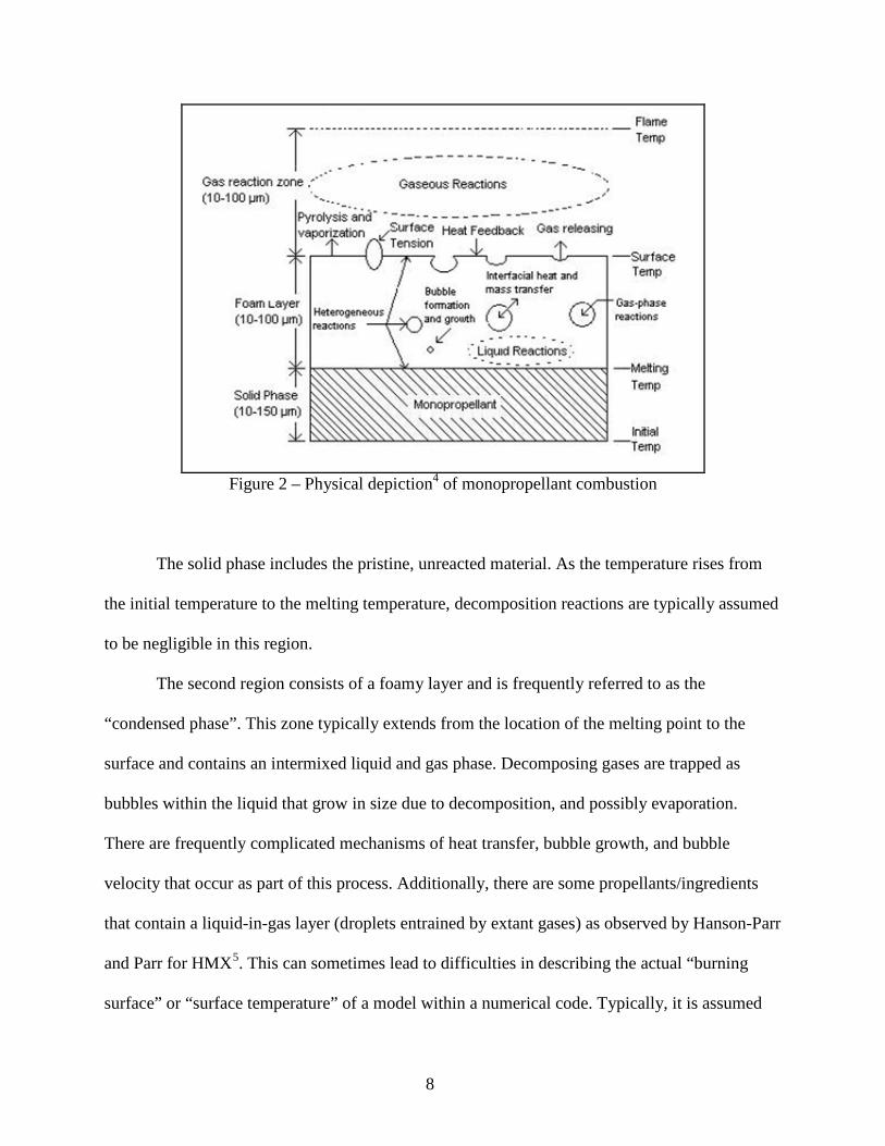
Figure 2 – Physical depiction4 of monopropellant combustion
The solid phase includes the pristine, unreacted material. As the temperature rises from
the initial temperature to the melting temperature, decomposition reactions are typically assumed
to be negligible in this region.
The second region consists of a foamy layer and is frequently referred to as the
“condensed phase”. This zone typically extends from the location of the melting point to the
surface and contains an intermixed liquid and gas phase. Decomposing gases are trapped as
bubbles within the liquid that grow in size due to decomposition, and possibly evaporation.
There are frequently complicated mechanisms of heat transfer, bubble growth, and bubble
velocity that occur as part of this process. Additionally, there are some propellants/ingredients
that contain a liquid-in-gas layer (droplets entrained by extant gases) as observed by Hanson-Parr
and Parr for HMX5. This can sometimes lead to difficulties in describing the actual “burning
surface” or “surface temperature” of a model within a numerical code. Typically, it is assumed

9
that there are no gas-phase reactions that occur within the condensed phase, although gas-phase
“bubble reactions” will infrequently be included as part of a condensed-phase description6,7
6
.
Reactions within the condensed phase are typically considered to be global or semi-global in
nature, as we know very little of what is actually happening in this region. Modern condensed-
phase reaction mechanisms contain relatively few reactions (on the order of ten, but sometimes
as few as one) and involve similar numbers of species -8.
In the gas phase region, the species evolved by the decomposing condensed phase react
toward final products and a final flame temperature while interacting with the condensed phase
through the following mechanisms:
1) the evolution rate of decomposed species from the condensed phase,;
2) the temperature of gases leaving the condensed phase;
3) conductively heating the surface of the condensed phase to due flame proximity.
Modern reaction mechanisms used to describe gas-phase chemistry contain tens to
hundreds of species and involve hundreds of reactions9
Early combustion models for propellants/ingredients were global in nature and only
contained rudimentary descriptions of kinetic processes. These models relied mostly on the
solution of the energy equation and were solved in a single dimension. Results from these
models showed that simply matching burning rate predictions to data was not enough to validate
a given model. An example of these early global models
.
10-13 that describes the combustion of
various propellants/ingredients was the BDP model14, which presented equations for solving the
thermal development of a combusting material. This model proposed that there is a limited
amount of energy available to the system with known beginning (initial) and ending
(equilibrium) conditions. The evolution of heat within the model could be described in a variety
of ways—with endothermic condensed phases followed by exothermic gas phases, or exothermic
10
condensed phases followed by exothermic gas phases—with the possible models being able to
accurately predict burning rate data regardless of the balance between the two. The important
restriction in determining the evolution of heat was that the initial and final conditions be correct.
More rigorous predictions of temperature sensitivity (change in burning rate for a
propellant/ingredient with a higher initial temperature—defined in Appendix A) and laser-
augmented burning rate can validate this kind of model to a greater extent, giving more
confidence in their accuracy. It is these predictions that require a more accurate description of
how a propellant/ingredient responds to a given application of heat. Understanding these
phenomena is the driving force for making these models more closely approximate reality.
As the science of modeling continued to develop and computing power multiplied,
complex gas-phase descriptions were coupled to simple condensed-phase models to try and
describe the combustion process of propellants/ingredients in greater detail. For these detailed
models, comparisons have been made between model predictions15
The BYU steady-state propellant/ingredient models were developed through the use of
the Phase3
and observed temperature
and species profiles above the burning surface. In making such improvements, it became
additionally important to match equilibrium species fractions as part of the final model
conditions.
16
Figure 2
computer program, which is named after the three regions of such a model
illustrated in . The most recent version of a gas-phase reaction mechanism for modeling
a large set of monopropellants and homogenous mixtures was developed at BYU by
Puduppakkam15 (for HMX8,16, RDX16, GAP15, BTTN15) and later expanded by Gross (to include
AP and ADN17). It contained 106 species and 611 reactions and is referred to as BYU’s
“universal” mechanism. The number of species involved in a gas-phase mechanism, which

11
affects the number of conservation equations in the solution process, and the non-linearity of
those reactions will typically dictate the length of time required for calculation. As such, robust
numerical techniques have been used within Phase3 to quickly and accurately solve the
necessary system of conservation equations. Phase3 uses a modified version of PREMIX18 in the
burner-stabilized mode for the gas phase solution and a modified version of DVODE19
02
2
=∂∂
−∂∂
xT
xTrc sbps λρ
for the
condensed phase.
In the solid-phase region of Phase3, the heat equation is included by implication,
according to Equation 1, and not included as part of the simulation calculations.
(1)
The liquid-gas foamy region includes the solution of the temperature, void fraction, and
species equations, while satisfying continuity through the assumptions that,
1) the momentum of the liquid is equal to the momentum of the gas (ρgug = ρlul);
2) the temperature of the gas and liquid within a discretized distance are equivalent;
3) the velocity of the liquid, ul, is equal to the burning rate of the propellant.
The equations describing the condensed-phase region comprise Equations 2 through 6.
( ) ∑=
+=∂∂ NumSpec
kkkcpc HACmA
x 1ωττλ (2)
τ=∂∂
xT (3)
( ) ∑=
=∂−∂ NumLiqSpec
kk
llux 1
11 ωρ
φ (4)
( )[ ] kklll Yux
ωρφ =−∂∂
,1 NumSpeck ...1, = (5)

12
[ ] kkggg Yux
ωφρ =∂∂
, NumSpeck ...1, = (6)
The second-order temperature equation has been split into two first-order equations for
ease of solution. The void fraction is calculated based on the global condensed-phase
decomposition reaction(s), and the gas and liquid species are solved separately. (i.e.: all gas-
phase species in the condensed phase sum to one, and all condensed-phase species sum to one.)
The equations describing the gas phase are given by Equations 7 through 10.
uAm cρ= (7)
RTWP
=ρ (8)
0111
, =+∂∂
+
∂∂
∂∂
−∂∂ ∑∑
==
NumSpec
kkkk
p
cNumSpec
kkpkk
p
cc
p
WhCA
xTCVY
CA
xTA
xCxTm ωρλ (9)
( ) 0=−∂∂
+∂∂
kkckkck WAVYA
xxYm ωρ NumSpeck ...1, = (10)
Ammonium perchlorate (NH4ClO4 or AP) is the most widely used propellant ingredient
in current production. It has been used for decades in applications ranging from the large space
shuttle booster to relatively small fighter-jet missiles. AP exhibits some of the most interesting
and complicated decomposition characteristics seen within the entire family of traditional
propellant ingredients.
2.1.1 AMMONIUM PERCHLORATE
At ambient conditions, AP is a crystalline salt with an orthorhombic structure that
changes to cubic at 513 K. It is a stable compound and can be grown into large crystals that are
centimeters in size or crushed and ground into particles that are microns in size. When AP
deflagrates, the resulting gases are very rich in oxygen (~30% O2, final products), and thus it is

13
typically mixed with very fuel-rich binders, resulting in excellent propellants. Additionally,
varying the size of AP particles within a propellant allows a unique method of control over the
propellant burning rate. Propellants formulated with fine AP burn more quickly, while those that
include coarse AP burn more slowly.
Years of study and research have been focused toward trying to understand the details of
AP decomposition and deflagration both as a monopropellant and when it’s contained within a
matrix of heterogeneous propellant.
2.1.1.1 LOW-TEMPERATURE DECOMPOSITION
At relatively low temperature, samples of AP undergo partial decomposition, a
phenomenon that is unique to this ingredient. In these experiments, AP crystals are heated at
either a very low rate or in an oven of constant temperature, typically ranging from 480 to 600 K.
Approximately 30% of every sample will decompose, at which time the decomposition rate
slows considerably. Vyazovkin and Wight20
Numerous other publications have tried to determine the decomposition pathways of AP
and the activation energies of these processes
have published a review of twenty different studies
of this phenomenon. The works included were conducted at low pressures (from vacuum to
atmospheric) and over a wide range of temperatures (from 475 to 750 K) using a variety of data
collection techniques. Decomposition ranged from 30% to 100% and activation energies from 70
to 260 kJ/mol were reported. The temperature range included the solid-phase temperature
transition at 513 K, and therefore the data included the orthorhombic phase, the cubic phase, and
partially-decomposed variants of each.
21-25 with similar results and significant data scatter.
The trends that have been observed suggest that the decomposition of both orthorhombic and
14
cubic AP initially proceed from pristine conditions to a state of partial decomposition (~30%), at
which time the rate drops appreciably but continues to completion.
Small-diameter AP particles have also been shown, however, to have partial
decomposition values that are significantly less than the ~30% observed in large crystals.
Beherens and Minier24 collected decomposition data at 0.3 psi, reporting 25% partial
decomposition for 200 micron particles and 13% for 20 micron particles. Kraeutle et al.26
2.1.1.2 STEADY-STATE WORK
also
saw this phenomenon to a limited extent in their work. Although no direct relationship between
AP particle size and extent of decomposition was given by Kraeutle, it was noted that under
some conditions samples of ground AP would decompose in the range of 25-35% before
slowing, and that AP ground to 3 microns didn’t decompose to any appreciable extent. It is not
understood why this occurs, but it does seem as if there is some kind of limiting phenomenon
that leads to the gradual disappearance of the low-temperature decomposition pathway as AP
crystal size decreases and the level of decomposition approaches ~30%.
Ammonium perchlorate can self-deflagrate above pressures of ~18 atm (300 psi). Below
this pressure, AP will not burn without assistance of some sort, be that through the addition of
heat, a kinetic catalyst, or additional fuel source. This pressure-deflagration limit (PDL) varies
with initial temperature as noted by Watt and Peterson27. At pressures higher than the PDL, AP
exhibits some very non-linear burning behavior, which has been divided into four suggested
pressure zones by Boggs28 Figure 3, as shown in alongside data from Atwood et al.29.

15
Figure 3 – AP experimental burning rate29 and defined regions of combustion28, Tinit 298K
The first region, which begins at the PDL and continues to ~54 atm (800 psi), can be
described by a simple burning rate relationship, rb ~ bPn, where P is the pressure of the system
and b and n are fitting parameters. Examination of the condensed phase from samples quenched
at steady-state burning in this pressure region (using techniques such as SEM) shows three
distinct structures of AP: the original orthorhombic crystal at the base of the sample, a layer of
unreacted cubic AP, and a thin film (1-5 microns28) of melted AP that is frothy and full of
decomposed gases.
SEM data from samples burned in the second pressure region, between 54 and 136 atm
(800 and 2000 psi), show the gradual disappearance of the melt layer and exposure of the cubic-
AP layer. The surface of the crystal in this region resembles a thumbprint with solid-phase ridges
and reaction-dominated valleys covering the entire surface. The ridges increase in height as
pressure increases. The burning rate in this region increases less rapidly than in region one but
holds to the same general description of burning rate: rb ~ bPn , with nRegII < nRegI.
The third and fourth regions, at pressures greater than 136 atm (2000 psi), exhibit
combustion that is incredibly erratic and unstable. Over this pressure range, the burning rate
drops drastically by nearly 80% and then rises again at a much steeper rate of change. Composite

16
propellants formulated with a fraction of AP, however, do not show this type of distinct behavior
at these pressures, and therefore accurately describing AP combustion in these regions is of little
practical importance.
Accurate experimental measurements of AP properties have been very difficult to obtain.
Thermocouples embedded in the solid crystal break at the 513 K phase transition as the structure
changes from orthorhombic to cubic. This has made it virtually impossible to determine the melt
temperature and/or surface temperature of a burning sample of AP through traditional means.
Additionally, the PDL at ~18 atm has made it difficult to obtain temperature and/or species
profile data within the gas-phase region above the burning surface, since these measurements are
usually collected at pressures less than 1 atm due to the very steep gradients of temperature and
species found during deflagration at high pressure. Current technology has not found a way to
yet resolve these steep gradients typically found at high pressure.
Other methods of detection, however, have been used to determine these important
physical parameters for AP. Beckstead and Hightower30 inferred the surface temperature for a
deflagrating AP crystal at pressures from 18 to 68 atm (300 to 1000 psi) to be somewhere
between 800 and 875 K through a thermal analysis of the measured depth of the cubic-phase
layer of quenched samples. They utilized the phase-transition temperature, experimentally-
observed thermal conductivity, and the assumption that the relationships governing thermal
conductivity in the cubic and melt phases were identical. Cordes31 estimated the melting
temperature of AP to be between 845 and 885 K, by comparing the melting temperatures of
similarly structured crystals. High-pressure compression data for crystalline AP under non-
combustive conditions have been extrapolated to pressures of interest by Foltz and Maienshein32
that suggest the onset of the crystalline melt could be as low as 600 to 675 K.

17
Ermolin et al.33 collected data at 0.6 atm from samples of AP preheated to 530 K to try
and resolve the species leaving the surface during deflagration. The low pressure allowed for a
longer gas-phase reaction zone and showed that decomposing gases were predominantly final
product species. Korobeinichev34 modeled this system with a gas-phase reaction mechanism
proposed by Ermolin et al.35
24
and reported that to predict the experimental species profiles
collected at 0.6 atm, the condensed-phase decomposition products of his model needed to be
approximately 20-30% final products (HCl, Cl2, N2, N2O, NO, etc) and 70-80% sublimation
products (NH3, ClO4) and intermediates (ClO2, ClOH). Behrens and Minier found
decomposition products from AP crystals heated to temperatures between 433 and 483 K that are
qualitatively consistent with Korobeinichev’s result.
Several AP burning rate models have been previously developed10-14 based on global
kinetics and containing a wide array of inputs. Price et al.36,37
37
compared their model and results
to the Beckstead-Derr-Price (BDP) model, the Guirao-Williams (GW) model, and the Manellis-
Strunnin (MS) model. The inputs between them vary significantly, the most pertinent to this
work being the condensed-phase heat release. BDP and GW assumed 30% sublimation, resulting
in an overall exothermic condensed phase. The MS model assumed 100% sublimation. Price et
al. used a condensed phase that varies from ~30% to ~80% sublimation, shifting the condensed
phase from exothermic to endothermic over the pressure range of 400 to 1500 psi. More recently,
new models have been developed for AP that include detailed kinetic mechanisms for the gas-
phase17,38
An AP model by Jing
-43. These models have only been applied to the two low-pressure regions of practical
interest (less than 136 atm).
41 made use of the Phase3 computer code and was of interest to the
current work. A five-step global kinetic mechanism was proposed to describe the condensed-

18
phase decomposition and predict steady-state surface species. His condensed-phase mechanism
is shown in Table 1.
Table 1 – AP condensed-phase decomposition reactions from Jing41 Reaction A [s-1] Ea [cal/mol] 4APc 3.25HCl+5.875H2O+4.146O2 +1.833N2O+0.375Cl2+0.33NH3
N/A N/A
APc NH3+HClO4 4.0∙1012 28,000 APc H2O+O2+HCl+HNO 1.0∙108 22,000 APc 2H2O+Cl+NO2 5.0∙107 22,000 APc ClO3+NH3+OH 1.0∙109 22,000
The first reaction accounted for 30% of the solid decomposition and was assumed to run
to completion before the onset of melting. This reaction took the place of the bubble reactions of
the earlier Beckstead and Tanaka44
Table 1
model. The remaining four condensed-phase reactions
described the completion of condensed-phase decomposition, though greater than 99% of this
remaining decomposition moved through the endothermic, sublimation reaction (reaction 2 in
). A gas-phase kinetic mechanism by Ermolin45,46
Table 2
containing 30 species and 79 reactions
was used. Thermodynamic properties used in Jing’s model are listed in . The model
accurately predicted burning rate from 20 to 100 atm and final flame temperature. Temperature
sensitivity predictions were within the upper range of the data.

19
Table 2 – AP properties used in the Jing41 AP model Property Value Chemical Structure NH4ClO4 ΔHf,298
47 -70.7 , [kcal/mol]
Molecular Weight, [gm/mol] 117.5 Phase Orthorhombic Cubic Liquid Density47, [gm/cm3] -- -- 1.76 ΔHtr
42, [kcal/mol] -- 2.5 7.0 Temperature range, [K] < 513 513 – 815 > 815
Heat capacity47, [cal/gm/K] Cp(T[K]) = 0.14 + T∙0.41∙10-3 (T < 513) Cp(T[K]) = 0.16 + T∙0.41∙10-3 (513 < T < 815) Cp = 0.49 (T > 815)
Thermal cond48 λ(T[K]) = 9.95∙10-4 – T∙3.75∙10-7 , [cal/cm/K/sec]
The recent work of Gross17 is most applicable to the current work. This was a steady-state
model built upon the work of Jing41 that used a single condensed-phase decomposition reaction,
as given in Table 3.
Table 3 – AP condensed-phase decomposition reaction from Gross17 Reaction A [s-1] Ea [cal/mol] 10APc 7O2+13H2O+3N2+4NH3+HCl+HClO4+Cl2+3ClO3+3Cl 3.0∙1010 28,000
Thermodynamic properties for Gross’s condensed phase were identical to those used by
Jing in Table 2. The gas-phase kinetic mechanism of Puduppakkam15 was modified to work for
AP by expanding it to include 106 species and 611 reactions. The expansion of the
Puduppakkam mechanism included adding several new reactions for NOCl, HCl, and several
nitrogen-hydrogen species from an ADN mechanism originally proposed by Liau et al.49 and
later modified by Korobeinichev et al.50. To achieve correct final nitrogen species concentrations

20
in the gas phase, and after trying several different approaches, Gross decided to increase the pre-
exponential rate factor for the reaction:
22 ONNO += (11)
by 6 orders of magnitude. In his work as well as in those that came before him at BYU, a very
large amount of NO was predicted to still be present in the final species fractions of several
different propellants/ingredients. In this case, Gross surmised that something was lacking in the
final gas-phase mechanism used for AP, and that this deficiency probably involved inadequately
describing the nitrogen-chlorine chemistry. Increasing the pre-exponential rate factor of the NO-
elimination reaction forced the model to predict equilibrium conditions for NO, N2, and O2 as
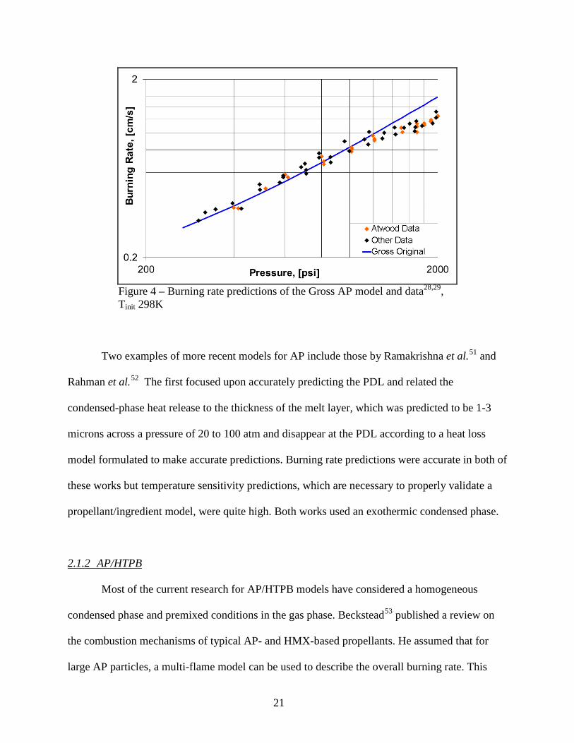
well as final flame temperature, which had previously been low by ~30 K. Gross’s final model17
was able to accurately predict burning rate from 20 to 100 atm (300 to 1500 psi) as shown in
Figure 4 with data from Boggs28 and Atwood29, temperature sensitivity, final flame temperature,
and final species fractions.
Predicted surface species fractions of the Gross model were closer than the Jing model to
those found by Ermolin et al.33. The heat release in the condensed phase for Gross’s AP model (-
42 cal/gm, exothermic) was also more consistent with other BYU monopropellant models, which
have condensed-phase heat releases ranging from +50 cal/gm, endothermic, to -150 cal/gm,
exothermic. The Jing model had a condensed-phase heat release that was +175 cal/gm,
endothermic. The melt layer thickness predicted by Gross’s model at 18 atm was 0.07 microns
and increased with increasing pressure. Both the value and trend of these predictions are contrary
to experimental data, which show that in the region from 18 to 68 atm (300 to 1000 psi), the
thickness of the AP melt layer is on the order of 1-5 microns28, the cubic layer in the range of 10-
30 microns30, and that each of them decrease with increasing pressure.
21
Figure 4 – Burning rate predictions of the Gross AP model and data28,29, Tinit 298K
Two examples of more recent models for AP include those by Ramakrishna et al.51 and
Rahman et al.52 The first focused upon accurately predicting the PDL and related the
condensed-phase heat release to the thickness of the melt layer, which was predicted to be 1-3
microns across a pressure of 20 to 100 atm and disappear at the PDL according to a heat loss
model formulated to make accurate predictions. Burning rate predictions were accurate in both of
these works but temperature sensitivity predictions, which are necessary to properly validate a
propellant/ingredient model, were quite high. Both works used an exothermic condensed phase.
Most of the current research for AP/HTPB models have considered a homogeneous
condensed phase and premixed conditions in the gas phase. Beckstead
2.1.2 AP/HTPB
53 published a review on
the combustion mechanisms of typical AP- and HMX-based propellants. He assumed that for
large AP particles, a multi-flame model can be used to describe the overall burning rate. This

22
description collapses to a single flame at low to moderate pressures if the particles are of
sufficiently small size and the gaseous products evolving from the surface of the propellant
approach premixed conditions.
Ermolin et al.54 developed a kinetic mechanism from their experimental data to describe
the combustion of AP/PB (polybutadiene) propellants, which had 35 species, 58 reactions, and
was based on Ermolin’s earlier work with AP. Ermolin55
Chorpening et al.
calculated kinetic parameters for the
gas-phase mechanism assuming simple bi-molecular reaction steps for the AP/PB system.
56 sought to gain understanding into the deflagration of thin AP/HTPB
sandwiches with a layer of HTPB binder between two layers of AP. They varied the binder
thickness and looked at the flame structure, burning rate, and UV-active species in the gas phase.
They also conducted numerical calculations of the gas phase that included a global mechanism of
5 species and 2 reactions. Knott and Brewster57
56
improved the model developed by Chorpening et
al. to more appropriately model AP/HTPB sandwiches. It was a fully coupled, periodic, steady-
state model that allowed for a free surface, solid phase boundary condition, and included
simplified chemical kinetics for the gas and condensed phases.
Jeppson et al7. developed a model for the steady-state, one-dimensional combustion of an
AP/HTPB propellant composed of fine AP, which was also of interest to the current work. They
assumed premixed conditions at the gas-phase inlet, and used a 44-species, 157-reaction gas-
phase mechanism in conjunction with a semi-global, ten-step, condensed-phase mechanism.
Their condensed-phase mechanism is presented in Table 4.

23
Table 4 – AP/HTPB condensed-phase decomposition mechanism from Jeppson7
Reaction A [mol, cm-3, s-1]
Ea [cal/mol]
HTPB1200c 2HTPB590c+2OH 1.0∙1010 11,300 HTPB590c 10C4H6+3CH4 2.0∙1011 12,500 HTPB590c+10APc15CO+10C2H4+3H2O+8HCN+10ClO2+2NO+29H2 3.0∙1011 14,500 HTPB590c+10APc14CO2+10C2H2+9HCN+10ClOH+NO2+36H2+H 3.0∙1011 15,000 HTPB590c+20HClO48CO+24CO2+24H2O+20HCl+5C2H2+CH4+5H2 1.0∙1012 15,000 APc NH3+HClO4 4.0∙1012 28,000 APc H2O+O2+HCl+HNO 1.0∙108 22,000 APc 2H2O+Cl+NO2 5.0∙107 22,000 APc ClO3+NH3+OH 1.0∙109 22,000 4APc 3.25HCl+5.875H2O+4.146O2+1.833N2O+0.375Cl2+0.33NH3 N/A N/A
The tenth step of his condensed phase mechanism is a pre-melt step in which 13% of the
initial AP mass decomposes (as observed by Behrens and Minier24 for 20 micron AP particles)
through a low-temperature decomposition pathway identical to Jing41. Thermodynamic
properties for AP in Jeppson’s model were identical to those used by Jing and can be found in
Table 2. Thermodynamic properties for HTPB used in Jeppson’s model are given in Table 5.
Table 5 – HTPB properties used in the Jeppson7 AP/HTPB model Property Chemical Structure (C4H6)40(OH)2 ΔHf,298
58 -170 , [kcal/mol] Molecular Weight59 1212 , [gm/mol] Phase Solid (< 523K) Liquid (> 523K) Density47, [gm/cm3] 0.88 0.88 ΔHtr
60 -- , [kcal/mol] 2.0
Heat capacity47,60, [cal/gm/K] Cp(T[K]) = 0.25 + T∙0.85∙10-3 (T < 523) Cp(T[K]) = 0.19 + T∙0.62∙10-3 (T > 523)
Thermal conductivity47, [cal/cm/K/sec] λ(T[K]) = 4.4∙10-4 + T∙1.3∙10-7

24
Burning rate versus pressure predictions from Jeppson’s AP/HTPB model7, given in
Figure 5, showed good comparison to Foster's data61 from 7 to 35 atm for an AP/HTPB
propellant with 20 micron AP particles.
Figure 5 – Jeppson AP/HTPB burning rate vs. pressure and Foster data61, Tinit 298K
Above 35 atm, the model over-predicted burning rate, suggesting that the premixed
assumption was no longer valid for 20 micron24 AP particles at those pressures. This divergence
from the premixed assumption is typically associated with significantly hotter diffusion flames
being present near the surface above the solid interfaces of AP and HTPB. These diffusion
flames are present for large diameter AP and at high pressures. The limits over which a premixed
model can be assumed to be valid are not well-defined, but they are more likely to be correct for
very small diameter AP and/or at relatively low pressure.

25
Jeppson’s model7 predicted experimental29,61 burning rates for an AP/HTPB propellant at
20.4 atm and an initial temperature of 298 K, with formulations ranging from 77 to 100% AP.
Final flame calculations were also made and are given in Figure 6.
Figure 6 – Jeppson AP/HTPB model predictions and data29,61 for 20.4 atm, Tinit 298K
Model predictions below 77% AP began to diverge from experimental data and were thus
excluded from reported results. It was assumed that a lack of carbon in the gas-phase mechanism
accounted for the divergence of the model’s predictions.
Further work on BYU’s AP/HTPB model was completed by Tanner62
7
to try and increase
the compositional range over which Jeppson’s AP/HTPB model could be applied. The final
model was significantly different than Jeppson’s, with a different mechanism in both the gas
(Gross’s17 version of BYU’s universal mechanism) and condensed phase (individual
decomposition reactions for several, specified propellant formulations). Tanner’s work focused

26
on developing the compositional range between 60% and 80% AP and included the three-
reaction, condensed-phase decomposition mechansim presented in Table 6.
Table 6 – AP/HTPB condensed-phase decomposition reactions from Tanner62
Reaction A [mol, cm-3, s-1]
Ea [cal/mol]
10APc 7O2+13H2O+3N2+4NH3+HCl+HClO4+Cl2+3ClO3+3Cl 3.0∙109 28,000 HTPB 20C4H6+6CH4+2OH 1.0∙1010 12,500 Formulation-specific AP/HTPB reaction, listed in Table 7 1.4∙1011 11,000
The AP reaction used was from Gross’s AP model, though the kinetic pre-factor was
decreased by an order of magnitude, from 3∙1010 to 3∙109 s-1, and the melt temperature was
decreased from 815 K to 800 K. No reasoning was given for either of these changes. Tanner’s
HTPB decomposition reaction is a combination of Jeppson’s7 two HTPB decomposition
reactions. The third decomposition reaction used by Tanner to describe the condensed-phase
reaction between AP and HTPB was determined by the formulation of the propellant. Each of
these AP/HTPB reactions was based upon the decomposition products he expected would be
present for a propellant with that composition, but not based explicitly upon any observed data.
Additionally, the species evolved from these condensed-phase reactions, when compared across
several formulations, were structured to follow the trends he expected as well. Thus, as the
mixture became more fuel-rich by reducing the amount of AP in the formulation, species like CO
and H2 were increased, while those like H2O and CO2 were decreased. The kinetic parameters for
each of these AP/HTPB decomposition reactions were identical to one another so as to maintain
consistency within the model. The proposed decomposition reactions for each of the six separate
formulations of the AP/HTPB propellant in Tanner’s model are given in Table 7, with the listed

27
species for each propellant formulation being divided into reactants and products and the
reaction parameters for all reactions being listed at the top of the table.
Table 7 – Specific AP/HTPB condensed-phase decomposition reactions by Tanner62
Reaction parameters for all reactions: A = 7.0∙1010, [mol, cm-3, s-1] Ea = 11,000, [cal/mol]
% AP
Reactants Products
HTP
Bs
AP s
C4H
6
CO
H2O
HC
N
N2
H2
CO
2
ClO
H
HC
l
CH
4
C2H
2
NH
3
HC
lO4
Cs
79.90 2 82 22 4 88 20 8 12 12 32 4 0 24 46 46 0 77.73 2 72 24 6 78 16 8 14 10 28 4 0 22 40 40 0 75.03 2 62 26 8 68 12 8 16 8 24 4 0 20 34 34 0 71.59 2 52 28 12 37 8 5 30 4 15 2 0 18 34 35 0 65.97 2 40 27 11 25 3 4 39 1 10 1 0 16 29 29 17 59.25 2 30 20 4 0 0 0 69 0 0 0 1 15 30 30 57
Tanner's model was compared to Foster's burning rate data63
Figure 7
for three formulations: 75,
77.5, and 80% AP. This comparison is given in . No comparison of temperature
sensitivity predictions to data was reported.
Using the high AP formulation data, Tanner fit his model at lower formulations through
an extrapolation of the final flame temperature predicted by equilibrium. Tanner’s final model
predictions fit both the actual (filled) and extrapolated (hollow) points, presented in Figure 7,
quite well.

28
Figure 7 – Predicted AP/HTPB burning rate by Tanner model and data63 for 6.8 and 20.4 atm
Final flame temperature and species fractions were also predicted very well, but the final
gas-phase mechanism included one artificial reaction that was introduced and tuned to allow the
final species fractions and final flame temperature to match equilibrium. This reaction is given
by Equation 12.
CNHHCN +→ (12)
In addition to his work with AP/HTPB, Tanner also attempted to model an aluminized
AP/HTPB propellant. To do this, inert aluminum was added to both the solid- and gas-phase
mechanisms with the thermal properties of the metal included as a function of temperature, as
given by the JANNAF tables64
. No aluminum reactions were included in either phase.
Comparisons to final flame temperature and species were poor. Tanner stated that this
discrepancy was possibly due to the fact that the aluminum was essentially acting as a large heat-

29
sink within the two phases, since no chemical reactions for aluminum were included in the
model. No temperature sensitivity predictions were reported for the aluminized propellant model.
Although aluminum will not be included in any of the steady-state modeling associated
with the current work, the properties of aluminum are introduced here because transient ignition
predictions for an AP/HTPB/Al propellant will be included in the presented results of the current
work. They are presented in Table 8.
Table 8 – Aluminum properties used by Tanner62 and the current AP/HTPB model Property Chemical Structure Al ΔHf,298, [kcal/mol] 0.0 Molecular Weight, [gm/mol] 26.98 Phase Solid (< 933K) Liquid (> 933K) Density64, [gm/cm3] 2.7745 2.5546 ΔHtr
64, [kcal/mol] -- 2.5583
Heat capacity64, [cal/gm/K] Cp(T[K]) = 0.144 + T∙1.58∙10-4 (T < 933) Cp(T[K]) = 0.281 (T > 933)
Thermal conductivity64, [cal/cm/K/sec] λ(T[K]) = 0.651 – T∙1.62∙10-4
2.2 IGNITION
Ignition events can occur through various means, but most often develop as a result of the
transient heating of an HE material by radiative, convective, or conductive means. Experimental
data are collected by applying heat to an HE material and observing the time at which a light
appears or the time at which complete combustion can still be attained after removal of the
applied heat. The results of such experimentation are usually plotted65
Figure 8
in a manner similar to that
shown in , for time to ignition versus energy flux. The actual positions and trends of the
lines, however, are dependent upon many factors.
30
Figure 8 – General effect65 of heat flux on time to ignition for propellants
In these experiments, a sample of propellant/ingredient is exposed to a heat source of
particular value. The applied energy flux first results in a period of inert heating of the sample,
which is followed by the beginning of decomposition reactions (first decomposition, FD) that are
usually endothermic or mildly exothermic in nature. The condensed-phase pre-ignition reactions
that follow, frequently, but not always, lead to light-producing reactions (first light, FL,
sometimes referred to as ignition in older references) above the surface of the sample.
Eventually, the sample will contain a sufficient amount of heat-producing reaction in the
condensed and gas phases to allow the sample to transition to steady-state burning when the
energy flux is removed. The point in time at which this transition can occur, without resulting in
extinguishment, is referred to as the go/no-go point. Experimentalists report go/no-go times as

31
the time at which 50% of the experimental samples successfully transition to steady-state
burning after removal of the energy flux. Samples heated longer than the go/no-go time can
transition to steady state (go), whereas samples heated for less time will extinguish (no-go).
Go/no-go times typically shorten as pressure increases. This effect is significant below about 5
atm of pressure66
2.2.1 MODELING AND EXPERIMENTAL WORK
and is bound at very high pressures by the time to first decomposition, or first
light, since inert heating is essentially independent of pressure.
Both Vilyunov and Zarko67 66, and Hermance published comprehensive reviews on the
ignition of the solid and condensed phases of various materials from both experimental and
theoretical viewpoints. Studies including both experimental and modeling work have helped us
better understand the details of the ignition process. Previous ignition models have varied in
complexity ranging from those including only very few equations of conservation and global
kinetics through those that solve a large number of conservation equations and include very
detailed kinetic mechanisms. A few of these models are discussed here.
Early work focused only upon the condensed phase. Vilyunov et al.68
67
performed a
statistical analysis of their solid-phase model and found that thermal conductivity, initial
temperature, and kinetics had the greatest influence on time to ignition. Vilyunov and Zarko
extended work done by Zeldovich concerning radiative ignition based only on the condensed-
phase solution with respect to one-dimension and time. They defined an expression that related
time to ignition that was primarily affected by the imposed heat flux.
Dik et al.69 calculated temperature profiles within a condensed substance that was heated
to ignition through an inert, opaque shield. Knyazeva and Dik70 conducted experimental and

32
modeling work to better refine an analytical model accounting for sub-optimal contact between a
condensed substance and a thermal shield. Zarko71
Further work included the simulation of both the condensed and gas phases in an ignition
system. Significant work towards understanding the ignition transients within various types of
rocket motors was conducted during the early 1990’s
compiled a summary review on irradiative
ignition and developed a model based only on the condensed phase. He proposed that ignition
had occurred only if the initiation of rapid exothermic reaction within the condensed material had
begun and if the fuel could transition to a steady-burning state.
72 74-77. Gheris and Price used a code that
coupled the condensed and gas phases to predict motor performance during ignition. Dik and
Selikhovkin78 developed a simple ignition model that tracked the maximum temperature through
the condensed and gas phases using a single value of heat flux at the surface. They had to assume
a value for surface temperature as a function of time to close the equations. Knyazeva and
Zarko79,80
Figure 8
developed a one-dimensional, unsteady, numerical model for the purpose of
determining the ignition criteria of homogenous, condensed substances. They reported that if an
external irradiative source, of magnitude greater than 37% of the un-augmented steady-state heat
flux, was applied to the energetic material, then the resultant ignition of the propellant would be
unstable and could extinguish upon termination of the radiative flux. This result is contrary to the
behavior typically seen in experimental data as described by , since there is no
extinguishment region at prositions above the go/no-go line. Their results could be applicable if
the time over which the energy flux is removed is taken into account within a given model, and
the kinetic assumptions of that model are accurate.
Huang et al.81 developed a four-phase model to predict the ignition capability of
nitramine-based propellants that were subjected to the impingement of a hot fragment of foreign

33
material (solid phase, liquid phase, gas phase, and hot solid fragment). They focused on reactions
occurring in the solid and liquid phases of the HE material. Yang and Liau82, Liau and Yang83,
and later Liau et al.84 presented work on a time-accurate RDX model that used detailed kinetics
to predict laser-induced ignition events. Their model solved the mass, energy, and species
conservation equations for both gas and condensed phases using a detailed 45-species gas-phase
mechanism. The gas and condensed phases were coupled through an iterative process that
converged on values of surface temperature and burning rate.
Atwood et al.85 has conducted a series of laboratory experiments on ignition data for
RDX to use as inputs to a transient combustion model that predicted the burning rate of HE
ingredients. Parr and Hanson-Parr86
Several sources of ignition data for AP/HTPB propellants and AP were available for
validation of model predictions. Atwood et al.
collected experimental data on the ignition/extinction of
RDX. In these studies, ignition occurred at a point in the gas phase away from the surface, and
then the flame sheet snapped back to a position close to the surface, quickly transitioning into
laser-augmented steady-state combustion. The removal of the laser determined the go/no-go data
presented.
65,87
Atwood et al.
have reported time-to-ignition data for neat
AP at 34 atm (500 psi) at two levels of laser heat flux. Initial sample temperatures of 298 K and
373 K are included in their results. They note that the time of apparent first-decomposition for
AP coincides with the go/no-go point within the uncertainty of their measurements, which is not
explicitly reported. This behavior is different from that observed for HMX and AP/HTPB
propellants, where the condensed phase melts and begins to react well before the go/no-go point.
65,88
65
have presented time to first decomposition and time to ignition (go/no-
go) for AP/HTPB propellants with formulations of 80% and 84% AP and a non-specified AP

34
formulation88 that is likely similar to the same formulation. It has been observed89,90
65
that
significant decomposition begins to occur in AP-based propellants after the 513 K phase change
of AP. Time to first-light and time to ignition for an AP/HTPB/Al propellant with 20%
aluminum was also included in their results .
Shannon91 presented a large array of time to ignition data for AP/CTPB propellants that
varied several parameters. He used an arc-image furnace to ignite the samples and looked at how
times to ignition varied with respect to applied heat, pressure, binder type, and additives. Sofue
and Iwama92
Ahmad and Russell
also presented ignition data for an AP/CTPB propellant (75% AP, 22% CTPB, 3%
additives) at sub-atmospheric and atmospheric pressures. In addition to varying pressure, they
changed the composition of the surrounding gas to ascertain its effects upon time to ignition and
reported go/no-go times for Ar < N2 < He at 160 torr. This trend is consistent with the idea that
gases with a higher thermal diffusivity will allow for increased conduction of heat away from the
surface of the propellant and thus lead to longer times to ignition.
93
Cain and Brewster
studied an AP/HTPB propellant of unspecified formulation (with a
small amount of nitramine) and measured ignition transients. They presented go/no-go times
using an Ar-ion laser (varying the wavelength from 250-800 nm) for energy fluxes of 25 to 125
W/cm2, reporting that approximately 90% of the incident energy was absorbed by the composite
propellant regardless of laser wavelength.
94 reported times to ignition for an AP/HTPB propellant with 75% fine
AP (2 micron). They studied the effects of adding up to 1% carbon upon the results, and also
showed that time to first light and time to go/no-go for this formulation of propellant diverge at
sufficiently high heat fluxes (~150 W/cm2).

35
2.2.2 MEREDITH IGNITION MODEL
Meredith and Beckstead95 developed a one-dimensional, time-dependent, numerical
model to predict the laser-induced ignition of HMX that was of primary interest to this work.
They used a detailed kinetic gas-phase mechanism of 45 species and 231 reactions and a
condensed-phase mechanism first proposed by Brill96 82 and later modified by Yang and Liau , as
presented in Table 9, with heat of reaction calculated at the melt temperature of 554.5 K.
Table 9 – HMX condensed-phase decomposition reactions used by Meredith95 Condensed-phase reactions ΔHrxn, [cal/gm] A, [s-1] Ea, [cal/mol]
HMXc 4CH2O + 4N2O -233 1013 34,400
HMXc 4HCN + 2NO + 2NO2 + 2H2O +133 1016.5 44,100
Thermodynamic properties for Meredith’s condensed phase were similar to those used by
Davidson16. Those that were different are given in Table 10.
Table 10 – HMX properties used in Meredith95 ignition model Property Value Chemical Structure C4H8N8O8, (H2CNNO2)4 Density97 1.9 , [gm/cm3] Phase β α δ Liquid ΔHtr
98 -- , [kcal/mol] 0.45 1.9 11.4 Klaser for CP-absorption99 5672 , [cm-1] 4800 1294 1165 Temperature range98, [K] < 388 388 - 439 439 - 554 > 554 Heat capacity47, [cal/gm/K] Cp(T[K]) = 0.0497 + T∙6.6∙10-4 Thermal conductivity47, [cal/cm/K/sec] λ(T[K]) = 0.0015 - T∙1.15∙10-6
GP absorption cross-sectional area100 CO2: 2.0∙10-22 , [cm2/molecule] HMXg: 5.59∙10-19

36
Meredith’s model solved a transient set of conservation equations for the gas phase,
which are presented in Equations 13 through 17.
( ) ( ) 0=∂∂
+∂∂ u
xtρρ (13)
( ) ( ) 034
=
∂∂
∂∂
−∂∂
+∂
∂+
∂∂
xu
xxP
xuu
tu µρρ (14)
034)( '''
2
1=−
∂∂
−
∂∂
+
∂∂
∂∂
−∂
∂+
∂∂
−∂∂
−∂∂ ∑
=g
NumSpec
k
kkk Qxu
xHVY
xT
xxuH
xPu
tP
tH µρλρρ (15)
( ) ( ) ( ) 0=−
∂∂
+∂
∂+
∂∂
kkkkkk WYV
xxuY
tY ωρρρ
NumSpeck ...1, = (16)
∑=
= N
i i
i
WYRT
P
1
ρ (17)
The condensed-phase description was based on the work of Erikson101
( )0=
∂∂
rur ccρ
κ
, which assumed
that all gas-phase species beneath the surface were dissolved within the solid (i.e. the gas is
trapped within the solid/liquid phase and moves with the same velocity). The equations used to
describe the condensed phase are presented in Equations 18 through 20.
(18)
0)exp(1 ''
1=−−
∂∂
∂∂
−∂∂
+∂∂ ∑
=
rKKqhWrTr
rrrTCu
tTC absabss
NumSpec
kkkkpccpc ωλρρ κ
κ (19)
kkk
cck
c WrYu
tY ωρρ =
∂∂
+∂∂ NumSpeck ...1, = (20)
The boundary conditions for Meredith’s model were:
1) an inlet flow condition at the beginning of the solid phase, which fed pristine HMX at initial conditions into the flow field;

37
2) temperature, momentum, and species flux conservation at the boundary between the condensed and gas phases (surface);
3) an outflow condition at the end of the gas phase, which allowed for the escape of gases assumed to be no longer changing with respect to temperature, momentum, or composition;
4) an applied heat flux at the surface of the condensed phase for laser-assisted combustion and ignition simulations.
Meredith’s condensed-phase code was written in Fortran and used an iterative method of
lines to solve the conservations equations of species and temperature. The gas-phase code was
written in Ansi C and used the PETSc102 libraries for solution. The gas-phase code solved the
continuity, momentum, energy, and species conservation equations by a non-linear, Newton-like,
Krylov sub-space method. Gas-phase properties and reaction rates were calculated using the
Chemkin103
Meredith’s results are compared to various sources of experimental data in
libraries.
Figure 9.
Figure 9 – HMX ignition delay versus heat flux of Meredith model95 and data, Tinit 298K
38
Meredith’s ignition model included the ability to model the transition from unsteady to
steady-state burning after the removal of the laser heat flux, as shown in Figure 10.
Figure 10 – Meredith95 HMX ignition predictions at 2 atm, 50 W/cm2 and transition to steady state
The primary source of ignition validation data comes from experimental time to ignition
versus applied heat flux. For these predictions, the laser heat was applied as a boundary
condition at the surface of the gas/liquid foamy layer. The model the predicted snap-back effect
observed by Ali et al.104
Figure 11
, where the gas ignites away from the surface and then propagates back
toward the surface (13.0 ms to 13.5 ms in ), and a dark zone during laser-augmented
combustion (33.8 ms in Figure 11).

39
Figure 11 – Meredith95 snap-back effect and dark-zone predictions for the HMX ignition model, 1 atm, 400 W/cm2
Steady-state predictions were validated by removing the laser heat flux after ignition was
achieved (39.8 ms to 48.9 ms in Figure 11) and running the simulations until all transients had
died out (60.2 ms in Figure 11). The model was also very accurate in predicting steady-state
burning rate, surface temperature, and melt-layer thickness versus pressure, as well as laser-
augmented burning rate and dark zone presence for laser heat-fluxes of less than 200 W/cm2 at
1 atm.
2.3 COOKOFF
Cookoff can be described as the thermal initiation of a device containing an energetic
material. Devices usually considered include ammunition, small rockets, missiles, and bombs.
These types of munitions come in many different shapes and sizes. For cookoff experiments,
bombs are generally self-contained and require no additional preparation, but the open nozzles of

40
rockets and missiles are plugged to avoid any impingement of external flames or direct heat to
the propellant material within the article as well as confining all decomposed gases. Cookoff has
been split into two sub-categories based on the intensity of the heating rate. Systems with a low
heating rate are referred to as slow-cookoff systems, and those that are heated relatively quickly
are called fast-cookoff systems. The current work was most specifically focused on fast-cookoff;
however, this literature review will first include a small amount of discussion concerning slow-
cookoff research for completeness.
Slow cookoff is characterized by monotonic heating rates of 3-4 K/hr
2.3.1 SLOW COOKOFF
1 resulting in an
almost uniform temperature rise throughout the system, despite the low thermal conductivity of
the explosive. When the explosive reaches a sufficiently high temperature, solid-phase
decomposition begins. Decomposition occurs throughout the solid, but positions below the
surface heat up more quickly than the surface itself, due to the typical radial or spherical
geometry of the propellant in the test article. Thus, ignition events usually occur within the solid
material. Containment of evolved gases and the advanced level of resulting decomposition
within the solid usually lead to very violent and destructive ignition events. Early experimental
work and modeling efforts by Creighton105 studied the “ignition temperature” and time to
thermal runaway (point at which heat cannot be conducted away quickly enough to avoid
exponential heat growth due to condensed-phase decomposition) in slow-cookoff systems. A
similar model was studies by Hobbs et al.106 and Baer et al.107. They each reported that slow-
cookoff predictions showed the initiation of ignition events to occur beneath the surface of the
explosive.

41
Fast-cookoff heating rates are on the order of 100 K/hr
2.3.2 FAST COOKOFF
1 but cover a wide range of values.
Externally applied fluxes at these heating rates are on the order of 0.1 to 25 W/cm2. This level of
heating rate coupled with the low thermal conductivity of HE ingredients results in only a very
small portion of the energetic material near the outer surface of the solid ever reaching an
elevated temperature. Gases evolved from condensed-phase decomposition are trapped and
heated within the localized region between the propellant and enclosing case, and the gases
eventually ignite. Gas-phase ignition events for these systems cause a rapid increase in pressure
and ultimate failure of the container, but are typically much less violent than slow cookoff
events.
Early fast-cookoff modeling efforts employed the codes originally developed for slow-
cookoff with modified boundary conditions. Baer et al.107 noticed that higher heating rates
resulted in the ignition of the system occurring near the heated boundaries, and that such events
coincided with the mechanical failure of the containment, as depicted in Figure 1. Erikson and
Schmitt108-110 conducted a series of modeling validations for their code against fast-cookoff
experimental data taken by Atwood et al.111
Jing
for spherical geometries with relative success. Time
to ignition and temperature of reaction were predicted by the Erikson model reasonably well, but
it was stated that more efforts needed to be taken to validate the mechanical properties and
chemical-reaction mechanisms.
41 developed two different models to predict fast cookoff. He assumed a zero-
dimensional model that did not take into account an actual gas phase, but treated the gas and
solid phases to be in the same space and ignored convection within the computational domain.
Jing’s second model (one-dimensional) included a description of both the condensed and the gas

42
phases but did not couple the two together due to numerical difficulties. His model showed that
the thermal wave became steeper when the incident heat flux was increased. The model’s
condensed-phase results compared well to an analytical model. No comparisons to experimental
data were made, but both his zero- and one-dimensional models matched the predictions of an
earlier fast cookoff model by Beckstead and Hendershot112
Meredith and Beckstead
.
3 extended their ignition model to predict HMX cookoff systems.
The equations for the gas and condensed phases were identical to those used in their ignition
model, as were the kinetic mechanisms and physical properties of HMX. The only differences
between their cookoff and ignition models were a coordinate transformation into radial space and
the following new boundary conditions:
1) zero inflow at the center of the cylindrical test article;
2) zero outflow at the end of the gas-phase domain;
3) heat flux equality across the boundary of the gas and steel shell;
4) heat flux application at the exterior of the steel shell. The model most importantly allowed for the coupling of the condensed and gas phases
that Jing’s41 cookoff model for HMX could not. The model predicted the pressurization of the
container, implemented variable time-stepping and mesh-refinement algorithms, scaled well
when used on parallel architectures, and showed the ability to allow for an increasing gap
between the HE surface and thermally-expanding steel shell. Meredith’s numerical results
showed excellent agreement with experimental data95 over a large range of heat fluxes, as
previously shown in Figure 9.
Cirro and Eddings113 conducted a small number of cookoff experiments to study the
thermal boundary layer at the HE surface/container interface. An important observation of these

43
experiments was the amount of damage done to the cookoff container for varying HE
configurations. The experiments performed showed a wide range of violence of explosion—the
most benign resulting in pressure bursts of the container and little damage to container, while the
most violent transitioned to detonation and left only small quarter-size pieces of the steel
container.
An important finding of Meredith’s work was the realization that it is the imposed heat
flux upon the surface of the propellant that dictates the time to ignition and not the heat flux
imposed at the external surface of the container shell. It was also reported that the time to
ignition of a fast-cookoff system was strongly dependent upon the width of the modeled air gap
between the HE and container. This is of particular interest because the model applied to the
external container was one that only calculated the thermal wave through the steel and did not
include the direct effects of dynamic pressure loading or thermal expansion upon the radius of
the heated shell. Meredith’s cookoff model investigated two separate means of approximating
the width of the air gap. The first was a constant width air gap. It was found that using values
between 0.5 and 1.0 mm resulted in the best prediction of the experimental data. Additionally, a
more accurate but entirely empirical method of determining the air gap width that was proposed
by Cirro and Eddings113 was employed in Meredith’s model. The results were much the same as
when using the constant gap width assumption, as the empirical equation had the air gap width
vary from 0.5 to 1.0 mm over the course of the simulation.
Finally, Meredith’s cookoff code was coupled to the post-processed, large-scale
simulation of a container within a pool fire3 through the heat flux to the surface of the container.
It was noted that applying the predicted heat flux from the fire simulation (which fluctuated
greatly with respect to time) to the surface of the container, resulted in essentially the same time
44
to ignition as a simulation where the average heat flux to the exterior of the container was used.
This was attributed to the dampening effect of the steel shell and led to significant simplification
of later simulations.
There were a few sources of experimental data found concerning the application of
AP/binder/Al propellants to fast cookoff systems. Ford et al.114
Wilson et al.
used an AP/HTPB/Al propellant
cast within the cylindrical portion of a large bullet-shaped test articlet that was placed within a
tube filled with flowing hot gases from the combustion of propane. The experimental apparatus
was designed to provide a constant heat flux to the cylindrical extermal surface of the test article
(radial coordinate system). The wall of the cylindrical test article was 3.175 mm thick 3140 steel.
Between the steel wall and the propellant was 0.762 mm of EPDM insulator and 0.762 mm of an
HTPB and carbon black liner.
115
Washburn et al.
used an AP/PBAN/Al propellant cast into a cylindrical casing that was
bolted over a table-hole, end-on. A propane/oxygen torch was placed beneath the table and
applied the incident heat flux according to the flame’s proximity to the end of the test article
(Cartesian coordinate system). At the heated end of the test article was a 12.7 mm thick steel
plate. Between this steel plate and the propellant was 2.54 mm of nitrile-butyl rubber insulation
and 1.42 mm of an unspecified polymer liner. Their work was initiated to extend the range of
heat fluxes to which AP/Binder/Al propellants had been applied in the past. Their data showed
times to ignition that were earlier than expected (low surface temperatures), but which were
consistent with other sources of data.
116 inserted an AP/Binder/Al propellant catridge into a cylindrical casing,
which was then attached to a plate, end-on, and exposed to radiant heating by a quartz lamp
(Cartesian coordinate system). The propellant was bonded by its radial surface to the casing by a

45
room-temperature vulcanizing (RTV) silicone adhesive. At the end of the heated article was a
1.47 mm thick steel plate. No insulation or liner was used between the propellant and steel plate,
though four thermocouples were placed there. Their results showed surface temperatures at
ignition that were more consistent with bare propellant data.
The bulk of the work that has been accomplished, as evidenced by the small collection of
data presented in this section, has only been collected within the past few years. Understanding
the science surrounding the prediction of cookoff events for composite propellants, such as the
one at the center of the current research, is very new, but has the propensity to be categorized and
better understood by propellant/ingredient modeling of steady-state conditions and bare surface
ignition events. Understanding how AP/HTPB/Al propellants respond to cookoff conditions is of
vital importance as a majority of the weapons and munitions in production today employ
propellants that are very similar in nature and formulation to those investigated by the current
work. The current work comprises one of the relatively few efforts in the literature being made to
better understand these propellants and how they respond to thermal stimuli so that any possible
accidents involving these potentially destructive propellants may be avoided.

46
47
Work and play are words used to describe the same thing under differing conditions.
-- Mark Twain
CHAPTER 3: OBJECTIVES
The primary goal of this work was to model an AP/HTPB/Al cookoff system by making
accurate predictions of time to ignition. Propellant ignition models are typically validated by
comparing to experimental time to ignition data. The models used to predict these data are based
on propellant/ingredient models that have first been validated by comparison to steady-state
deflagration data. The current work involved a rigorous attempt to verify and validate the time-
to-ignition of cookoff events by investigating each level in the structure of the complete model
and code and then identifying wherein they each needed to be improved. In doing so, several
updates were made to both the models and the codes that employed those models. The end goal
was not only to make meaningful predictions but to have confidence in those predictions as well,
or at the very least to define a path by which confidence might be attained. Knowledge and
understanding were of primary concern to the current work and provided a singular drive toward
its completion.
This project began at the ending point of the work accomplished by Meredith and
Beckstead3,95 and the ignition code developed by them, as well as the ending points of the
propellant/ingredient models of Gross17 and Tanner62. Several different sub-projects were
accomplished as part of the current work, each of which fell into one of two categories:
1) code improvement;
2) propellant model improvement.

48
The first of the coding projects was to generalize the ignition code with regard to the
simulated propellant/ingredient. When initially written, the ignition code was built for the single
propellant ingredient HMX. The condensed-phase portion of the ignition code, which had
originally been written in Fortran, also needed to be translated into Ansi-C to make a clean
integration between the ignition code and several other external software packages.
The second code-development project involved removing the use of Chemkin in the
ignition code. In February of 1997, the open-source Chemkin libraries were licensed to Reaction
Design117. As part of this process, a restricted license was grandfathered to all those with a
current version of Chemkin II or earlier, but the proliferation of the Chemkin II libraries to new
sources was restricted. To keep the ignition code free of charge for all users (including industrial
contacts that had no previous access to Chemkin II), Chemkin needed to be removed from the
code and replaced with a comparable open-source package. Cantera118 is a C++, open-source,
chemistry and thermodynamics package that was available at the initiation of the current work.
This set of libraries was developed by Dave Goodwin at Cal Tech. It was able to calculate the
thermal properties and reaction rates needed by the ignition code as accurately as Chemkin II,
and it had also been shown to make its calculations up to 40% faster.
The steps involving the improvement of the several propellant/ingredient models of
interest were structured such that each piece built upon the foundation of the work that had come
before it. Thus, the individual propellant/ingredient models were first validated against steady-
state data, then compared to laser-augmented data, and last to time-to-ignition data. Building a
validation structure in this way provides for a high level of confidence when making predictions
for the complicated details of ignition and cookoff at which a limited amount of experimental
data has been collected.

49
The several tasks that needed to be completed were:
1. Re-validate ignition predictions for the HMX model using the improved ignition code
2. Update Gross’s steady-state AP model using current literature resources
3. Validate the updated steady-state AP model, making changes if necessary
4. Validate laser-augmented predictions for the AP model
5. Validate ignition predictions for the updated AP model, making changes if necessary
6. Update Tanner’s steady-state AP/HTPB model using current literature resources
7. Validate the updated steady-state AP/HTPB model, making changes if necessary
8. Validate laser-augmented predictions for the AP/HTPB model
9. Validate ignition predictions for the updated AP/HTPB model, making changes if necessary
10. Validate ignition predictions for the AP/HTPB/Al model
11. Validate cookoff predictions for AP/HTPB/Al model
Steps two through nine of the above list fit into a validation structure for the new
propellant/ingredient models in various modeling configurations that have been included in the
current work. This validation structure is succinctly described by Figure 12.
Figure 12 – Proposed validation structure for the current work

50
Figure 12 lists the most complicated predictions of the current work (cookoff)—for
which we have the least data—at the top right, and the most simple (steady-state AP)—for which
we have the most data—at the bottom left. Predictions that are lower and to the left in the
validation structure are not only simpler but provide a foundation for making predictions with
confidence in regions that are higher and to the right.

51
You can't depend on your eyes when your imagination is out of focus.
-- Mark Twain
CHAPTER 4: CODE AND MODEL IMPROVEMENTS
The current work included the modification/improvement of two computer codes—the
steady-state propellant code, Phase3, and the ignition code developed by Meredith—and the
validation of several propellant/ingredient models applied to those codes (HMX, AP, and
AP/HTPB). The ultimate goal was to predict the combustion characteristics of these
propellants/ingredients under steady-state and laser-augmented conditions within Phase3 so that
the models could then be applied toward predicting ignition events, fast cookoff events, and the
transient changes that accompany each within the ignition code. Additionally, it was intended
that the ignition code be used to validate an AP/HTPB/Al propellant model for ignition and
cookoff events. Improvements made to the computer codes and propellant models, which had all
been previously developed at BYU, will be discussed in this chapter.
4.1 PHASE3 CODE IMPROVEMENTS
Two major improvements were made to the Phase3 code so that the current work could
be completed. The first was to allow for the inclusion of phase transitions within the modeled
domain of the condensed-phase. Prior to this work, the only portion of the condensed phase that
was explicitly calculated was the melt layer. All temperature-based phase changes and the energy
associated with each were accounted for prior to beginning the condensed-phase calculation of
the melt layer. Phase changes that had been defined at temperatures above the melt temperature

52
were not included in the calculations. During the development of the AP model for the current
work, the desire arose to compare predicted cubic-layer thickness to experimental data.
Condensed-phase calculations were therefore made that included a domain of temperatures lower
than the melt temperature. Thus, the method of calculation needed to be changed such that
temperature-based phase changes, and the energy associated with each of them, could be
accounted for regardless of the temperature at which the condensed-phase calculations began.
Additionally, to implement the final version of the current AP model, which will be discussed
later, it was necessary that the code also be able to make transitions between individual phases of
a propellant ingredient (e.g.: orthorhombic AP, cubic AP, and melted AP) such that different
regimes of kinetic decomposition for a single ingredient (AP, in this example) could be
described.
The second improvement made to the Phase3 code was to add the ability to model the
penetration and absorption of a laser into the condensed-phase domain for a laser-augmented
case. Previously, the only option to model laser-augmented combustion within Phase3 was to
treat the laser as a boundary condition at the defined surface of the propellant. This assumption,
though used rather frequently in modeling efforts is far from accurate for AP, an ingredient that
is highly transparent to the wavelength of laser light typically used (~10.6 microns). AP is
different in this regard from most other propellants/ingredients, which are essentially opaque to
the laser light. This sub-model was fairly difficult to incorporate into the code because the
condensed-phase solver employs a shooting-method that calculates the solution profiles from the
cold side of the propellant toward the hot, whereas the absorption of the laser has to be calculated
from the hot side of the propellant toward the cold. After numerous trials, an iterative method

53
was developed to converge upon the location of maximum absorption that worked sufficiently
well.
4.2 IGNITION CODE IMPROVEMENTS
Several improvements were made to the ignition code over the course of this work. The
first involved the replacement of the Chemkin libraries with Cantera. This effort was a straight-
forward process, as each call to Chemkin from the initial version of the code had an analogous
call to Cantera. A comparison between the two versions of the ignition code was made. Rates
and properties returned from Cantera were within less than 1% of those calculated by Chemkin,
and required less time to calculate as well. Both Cantera and Petsc, the numerical solver library
used by the ignition code, were kept up to date with current releases of the software. As of the
completion of the current work, the ignition code was using Cantera 1.8.0 and PETSC 3.1-p7.
Many changes were also made to the condensed-phase portion of the ignition code. The
first involved translating the code from Fortran into Ansi C. The decision to do this was made for
two reasons: the first, to simplify the integration of Cantera libraries into the code, which was
developed in C++; the second, because it was believed that doing so would simplify the
development process, which it did to considerable effect. The completion of this work led to an
in-depth analysis of the ignition code in general, which led to further correction of a number of
issues that the code was exhibiting when the current work was first begun. These issues
concerned general convergence, accuracy, memory overflow/overwriting, and the proper
integration of external library software packages.
Another change to the condensed-phase portion of the ignition code was to make the
condensed-phase equations and assumptions consistent with those of Phase3. Initially, there were

54
a few major differences between the two, and it was thought that comparisons between the
results of each would be more consistent with one another if these differences were removed. As
such, calculations for all species profiles within the condensed-phase portion of the ignition code
were changed to be calculated separately for liquid- and gas-phase species (e.g.: all liquid-phase
species fractions sum to one and all gas-phase species fractions sum to one within the condensed
phase). This change necessitated the addition of an accurate void fraction to the calculations of
the condensed-phase, which is given in Equation 21.
( )[ ] ( )[ ] ∑
=
=∂
Φ−∂+
∂Φ−∂ NumLiqSpec
kkx
ut 1
11 ωρρ (21)
This equation was discretized as up-winded, identical in manner to the species mass
fraction equations. Additionally, condensed-phase properties, which were originally based only
on the solid-phase species, were updated to include the effects of decomposed gases as well.
Physical properties for the condensed phase of both codes are now functions of temperature,
composition, and void fraction.
Another change made to the condensed-phase portion of the ignition code involved the
species convergence and progress of a simulation. Temperature convergence had always been
fast and robust, but the species convergence was extremely slow and determined on an absolute
basis. When the sum of the change of all species totaled a value that was lower than a defined
criterion, the condensed phase was determined to be converged. This criterion is given in
Equation 22.
( ) ConvCritYprevYnewTotNodes
i
NumSpec
jjiji <−∑ ∑
= =0 1,, (22)

55
It is more commonly held that convergence on a relative basis is more robust than an
absolute one. The new convergence of species, void fraction and temperature (all represented by
Φ) is now determined by Equation 23.
Max ConvCritprev
prevnew
ji
jiji <
ΦΦ−Φ
,
,, NumSpecjTotNodesi 1,0, == (23)
The convergence of the condensed phase was also altered so that its effect upon the
progression of the simulation would be minimized. Wall-clock calculation time for a given
simulation time step is typically dominated by the gas-phase calculations (typically, 90% or
more). Originally, any difficulty in the condensed-phase convergence was reduced by decreasing
the time step for the entire solution. This resulted in the overall calculation time being increased
significantly due to an insignificant contributor to wall-clock time. To avoid this, a multiple time
step method was added to the condensed-phase solution code. This allowed for the condensed
phase to take multiple time steps for each single time step of the gas phase, and has been
implemented so that the number of condensed-phase time steps taken for each gas-phase time
step is dictated by the difficulty of the condensed-phase solution.
Additionally, the means of transitioning one condensed-phase species into another, as
was mentioned as being implemented into Phase3, was integrated into the condensed-phase
portion of the ignition code. This process was significantly more involved for the ignition code
than it was for Phase3 due to the nature of the condensed-phase solution for the ignition code.
Current implementation transitions “adjacent” ingredient forms (eg. orthorhombic AP and cubic
AP at 513 K) across a 10 K window of temperature and across a 2% void-fraction window for
adjacent ingredient forms that transition at a particular void fraction. (i.e.: A temperature
transition at 513 K is linearly interpolated across a temperature range from 508 to 518 K, and a
decomposition transition at a void fraction of 0.3 is linearly interpolated across a void-fraction of

56
0.29 to 0.31.) Using a temperature window smaller than this (10K) for the current AP model
resulted in an oscillatory solution due to the very exothermic initial step of the condensed-phase
decomposition. The coding for this transitional ability had to be implemented individually for
each ingredient and was accomplished for the HMX, AP, AP/HTPB, and AP/HTPB/Al models.
If any future work on other propellants/ingredients needs to use this transitioning capability
within the ignition code, either the current coding would have to be generalized in some way or
additional code would have to be similarly developed to handle those new
propellants/ingredients.
The largest and perhaps most glaring difference between the steady-state and ignition
codes was the assumption as to when the effects of condensed-phase reactions were included. In
Phase3, condensed-phase reaction rates are not calculated below the melt temperature. This
assumption was consistent with numerous other modeling efforts. The ignition code, however,
needs a finite reaction rate to be calculated throughout the entire condensed phase due to the
mass flow rate of evolved species being important to both the condensed- and gas-phase
solutions at each time step.
In Phase3, the calculated reaction rate of condensed-phase components is dependent upon
both temperature and void fraction. The melt temperature condition occurs at a single position in
the condensed phase and does not change unless the inputs/conditions change. The point at
which the melt temperature criterion in the ignition code is met occurs first at, or near, the
surface of the propellant/ingredient and then propagates back into the solid as the melt layer
develops over time. As such, the rate of decomposition throughout the condensed phase at a
given location varies over a large range for a given simulation. Employing a method of solution

57
where the reactions are “turned on” at a particular temperature, as is the case for the Phase3
code, is difficult because of the numerical instability associated with such a change.
Three means were determined by which this discrepancy between the two codes might be
alleviated.
1) ignore the differences, using the reaction parameters from the steady-state model directly,but calculate them at all temperatures;
2) re-fit the condensed-phase kinetic parameters of the model in Phase3 by including the entire condensed phase in the calculations (above the initial temperature instead of just above the melt temperature), and then apply those new kinetic parameters to the ignition code;
3) ramp the reaction rate values gradually within the ignition code, once they are “turned on” at the melt temperature, to try and alleviate any possible numerical instability.
The first of these options was employed by Meredith during the initial development of
the HMX ignition/cookoff model. His results showed that this was a decent assumption for
HMX, with less than 5% of the simulated propellant decomposing or evaporating prior to an
ignition simulation reaching the defined melt temperature. Using this option for the AP model,
however, resulted in the ignition code never reaching the defined melt temperature due to
sufficiently-high reaction rates being predicted in the orthorhombic and cubic phases, which is
inconsistent with what has been observed for AP28. This seemed to imply that the difference
between the kinetics of orthorhombic/cubic AP and melted AP were probably more than 2-3
orders of magnitude apart, an assumption employed by the Phase3 code due to observations
similar to that of Behrens and Bulusu119
Efforts made as part of the current work to find new kinetic parameters for AP using the
second option were also unsuccessful. Thus, the third option was investigated and a logarithmic-
for RDX. Thus, using the method of Meredith in
applying the HMX model to the ignition code in a manner different than that employed by
Phase3 would not work for AP.

58
interpolation scheme was ultimately developed as part of the current work for the purpose of
minimizing the numerical instability involved in turning on the condensed-phase reactions at a
defined temperature. At each time step, the condensed-phase decomposition is checked at each
node to see if it has more than doubled since the previous time step. If it has, then the
decomposition is ramped for up to 200 time steps from that point, based on the level of disparity
between the decomposition at the previous time step and the decomposition predicted for the
current step. Ramping the decomposition solution in this way was very successful in predicting
minimal sub-melt decomposition while still allowing for numerical convergence of the
condensed-phase equations once the melt temperature criterion was reached.
Another problem with the original ignition code was that it was developed specifically
for HMX. The code itself contained variables and arrays that were dimensioned and organized
for the HMX reaction mechanism and were thus not directly compatible with reaction
mechanisms for other ingredients. The code was generalized as part of the current work to allow
for different properties and/or reaction mechanisms.
There were a number of issues that dealt with the convergence of the ignition code that
were also addressed. For example, the first several time steps of a simulation would typically
require a large number of non-linear iterations. The code would also typically diverge if the gas-
phase solution for a particular time step took more than five non-linear iterations. Restart cases
had frequent difficulty for ignition simulations, with cookoff simulations always diverging. Also,
cases defined with a high number of gas-phase nodes or large number of species (as is the case
for the current AP/HTPB gas-phase kinetic mechanism), would typically diverge immediately. It
was found that two coding errors led to the sum of these oddities.

59
The first was a discrepancy between the size (in memory) of variables being passed into
subroutines (mostly Petsc subroutines, but some within the subroutines of the ignition code
itself) that was not being caught by the compiler. This error was corrected as part of the current
work. The second issue dealt with an incompatibility between the Cantera and Petsc libraries.
The Cantera installation included a partial implementation of the BLAS and LAPACK numerical
libraries that was different than the version used to build the Petsc libraries. This was resolved by
specifying that the Cantera installation use the version of BLAS and LAPACK that was used
when building Petsc. To all appearances, the incompatibilities between these two software
packages have been resolved.
Two additional changes were made to the ignition code to allow for the inclusion of
aluminum in the modeled propellant. The first deals with the calculation of the thermal
conductivity of a propellant when aluminum has been added to the formulation, and the second
deals with the reflection of laser light from aluminum particles within the propellant.
The modeled effect of aluminum particles on the thermal conductivity of an AP/HTPB/Al
propellant is calculated by applying Maxwell’s approximation120
for the effective thermal
conductivity of a sphere surrounded by a continuous medium. The aluminum particles are
assumed to be spherical in shape, and the AP/HTPB propellant is assumed to be a continuous
phase surrounding the aluminum spheres. Maxwell’s approximation is given in Equation 24.
−
−+
+=
SCMS
CMS
SCMeff
kkkk
kkφ
φ231 (24)
This approximation treats the effect of aluminum upon the thermal conductivity of the
propellant as a deviation from the thermal conductivity of the continuous phase, AP/HTPB, and
60
is dependent upon the volume fraction (but not size) of aluminum in the modeled propellant. The
validity of this approximation will be discussed in Chapters 4 and 5, where it has been applied to
the current AP/HTPB propellant model.
The second effect that the addition of aluminum has upon a propellant, both modeled and
experimentally, is an increased ability to reflect laser light. Since most sources of current ignition
experimentation are handled with laser-light, this effect needed to be considered.
The size of aluminum particles used within propellants typically fall into the range of 1-
100 microns in diameter, while the wavelength of laser light from a CO2 laser is 10.6 microns.
The similar size between particle diameter and wavelength of light leads to a particle-light
interaction referred to as Mie scattering. The determination of how particles and light waves
interact under these conditions is a non-trivial, previously-solved problem121
1) reflection, or backscattering;
. Incident light
waves interacting with a solid, spherical, aluminum particle can produce one of three effects:
2) absorption;
3) forward scattering.
The numerical results of a computer program, Bhmie-c122, which was written using the
algorithm of Bohren and Huffman, was applied to the calculations of the current ignition code to
determine the extent of each outcome for incident laser-light interacting with the aluminum
particles present in the modeled, semi-transparent propellant. No absorption of laser light by the
aluminum is considered in the current ignition code.
The reflection sub-model in the ignition code was built upon a three-dimensional analysis
of a uniformly-structured propellant and then applied to a modified version of the laser-
absorption sub-model. In the current reflection sub-model, the size of a characteristic cube of
61
propellant is determined by setting the ratio of the volumes of a sphere and a cube (with the
sphere assumed to be completely contained by the cube) using the volume fraction and particle
diameter of the included aluminum. The single dimension of this characteristic cube is calculated
by using Equation 25.
31
3
6
=
AL
ALcube
dXφ
π (25)
This characteristic dimension dictates the coverage of aluminum across a projection of
the top of the cube (effective area of aluminum coverage, as viewed by the laser light and
calculated by using Equation 26), and also the depth of propellant present before another
characteristic cube will be reached by penetrating laser light.
2
2
4 depth
ALAL X
dAF π= (26)
These two dimensions are illustrated in Figure 13.
Figure 13 – Characteristic cube used in aluminum-reflection sub-model

62
Laser light incident upon the area fraction covered by the aluminum spheres is either
back-scattered or forward-scattered according to the calculations made by the Mie code. The
fraction of back-scattered light at the surface is considered to be reflected away from the
propellant and lost. The fraction forward-scattered at the surface is added to the fraction of the
laser falling outside the area of aluminum coverage, which sum total is then allowed to penetrate
into the propellant. The laser light is absorbed into the propellant according to the current laser-
absorption sub-model to a distance of Xdepth. At this depth within the modeled propellant, a new
characteristic cube is reached, and the process is repeated. For successive layers of characteristic
cubes, the area fraction of aluminum is assumed to not overlap that of previous layers. Thus, the
maximum depth to which the sub-model calculates aluminum reflection is: Xdepth/AFAl. Light
reflected at sub-surface depths is assumed to be absorbed by the propellant as it travels back out
of the propellant/ingredient. Since tens of thousands of characteristic boxes make up the modeled
surface of a propellant, this approximation is assumed to be valid. An illustration of the complete
aluminum-reflection sub-model is given in Figure 14, where the amount of incident laser light
for each layer is equal to the sum of reflected and forward-scattered fractions at that level.
Figure 14 – Physical description of the aluminum-reflection sub-model

63
Laser light still present as a forward-scattered fraction after the entire cross-sectional area
of the top of the characteristic cube is complete was typically a small fraction (< 15%) of the
overall incident laser light at the surface of the propellant and was assumed to absorb into the
propellant at greater depths without further particle interaction. This is consistent with the
assumption that none of the laser light allowed for by the current sub-model that makes it to this
depth will be able to back-scatter up to the surface and escape.
This implementation of light scattering due to aluminum particles has only been
implemented within the condensed phase equations. Part of the results of the current work
suggested that aluminum reflection of particles within the gas phase might be of importance
during the transition of an ignition simulation to an augmented steady-state solution. This period
of time for relatively high heat fluxes, however, involves the melting, conglomeration, and far-
surface ignition of the aluminum particles. None of these effects have been considered by other
models in literature to our knowledge, and thus they have not been considered as part of the
current work either.
4.3 IMPROVEMENT OF THE STEADY-STATE AP MODEL
The propellant/ingredient model modifications sparked a majority of the updates to the
computer codes that have previously been described. Improvements were made to the steady-
state AP model with two distinct directions in mind. The first involved the extension of Gross’s17
original model to include updated sources of input from the literature, and the second was a
complete re-thinking of the AP model to try and better describe the steady-state data.
The work associated with these two efforts fell beneath the wider goal of validating the
AP model for laser-driven ignition events. To make laser-driven ignition predictions with
64
confidence, the steady-state AP model needed to be able to predict not only steady-state
combustion, but laser-augmented combustion as well. Being able to accurately predict the laser-
augmented burning rate is important because it is an “ending point” for the transient, laser-
augmented simulations in like manner to the final flame temperature being an “ending point” for
steady-state simulations. In each case, the ending point is the goal at which simulations need to
arrive to be considered a valid description of simulated combustion.
4.3.1 PART 1: UPDATING AND OPTIMIZING THE GROSS MODEL
The main changes to the model inputs used by Gross in part one were to:
1) update the thermal properties of AP based on recent measurements of Parr123
2) decrease the melt temperature from 815 K to 735 K to keep cubic-layer thickness predictions consistent with measurements from Beckstead and Hightower
;
30;
3) update BYU’s “universal” gas-phase mechanism for propellants by updating 14 reactions and adding 35 new reactions according to the ab-initio calculations of Lin et al.124,125
. (Listed in Appendix D.)
After the above-outlined changes were made to Gross’s model, the pre-exponential of the
original condensed-phase reaction needed to be decreased by a factor of 20 to again predict the
steady-state burning rate. To better understand the need for this change, the relationship between
the condensed-phase pre-exponential and the predicted burning rate is shown in Figure 15 for
both the original Gross model and the updated model for a pressure of 68 atm (1000 psi).

65
Figure 15 – Predicted burning rate range for variations of Gross17 AP model and data29
Gross’s original AP model17 allowed for accurate burning rate predictions to be achieved
at two separate values of condensed-phase pre-exponential rate constant. The updated model,
which was completed as part of the current work, only allowed for a single intersection between
the model’s predictions and experimental data when using Gross’s original condensed-phase
decomposition reaction. Changing the pre-exponential rate constant for the updated model
caused a few large changes to the predictions.
The melt-layer thickness prediction at 18 atm (300 psi) increased from 0.07 microns
(original model) to 0.89 microns (updated model). Although this change was in the right
direction, 0.89 microns is still less than the 1-5 micron layer that was observed by Boggs28.
Predicted burning rate versus pressure for the updated model was decent when compared to
data28,29 (Figure 16), but the predicted temperature sensitivity was significantly higher than the
data29,37 (Figure 17).

66
Figure 16 – Predicted burning rate for variations of Gross AP model and data28,29, Tinit 298K
Figure 17 – Predicted temperature sensitivity for variations of Gross AP model and data29,37
The increase in predicted temperature sensitivity came as a result of decreasing the
condensed-phase reaction pre-exponential. For surface reaction models, the condensed-phase

67
kinetics do not affect temperature sensitivity predictions. For in-depth condensed-phase reaction
models, however, the condensed-phase kinetics cause some variance in the temperature
sensitivity predictions. This variation for the original Gross model17, which was as large as
100%, is shown in Figure 18.
Figure 18 – Variation of predictions for Gross AP model, 68 atm
The shift in temperature sensitivity predictions for the updated AP model was
concerning, since the accurate prediction of temperature sensitivity is a main point of validation
for all propellant/ingredient models.
Of additional concern was that the predicted laser-augmented burning rates of both
Gross’s original model and the updated model were too high by ~100% when compared to
data126
Figure 19
-129 and differed from each other by less than 3%. Laser-augmented burning rate
predictions using Gross’s original model are shown in .

68
Figure 19 – Predicted laser-augmented burning rate of Gross AP model and data126-129, 1 atm
Gross’s original model was never applied to laser-augmented combustion, and so the
discrepancy here is not surprising since making these kinds of predictions was not of primary
concern to his work. The fact that laser-augmented predictions from the updated model changed
by less than 3% was unexpected. A large parametric study was performed on the condensed-
phase inputs to determine what could be done to better predict laser-augmented burning rate. It
was found that the only parameter that made a significant impact (> 5%) upon these predictions
was the heat release in the condensed phase. This is due to the fact that changing the condensed-
phase heat release directly impacts the surface heat flux, and a change in the surface heat flux
directly affects the impact of a given level of laser-heat applied at the surface of AP. For
example, a laser heat flux value of 100 cal/cm2/s will more significantly affect a model with a
nominal surface heat flux of 50 cal/cm2/s (200% increase) than it would a model with a nominal
surface heat flux of 200 cal/cm2/s (50% increase).

69
The predicted final species fractions of the updated model changed very little from that of
Gross’s original model. One of the main reasons for updating the gas-phase mechanism was to
remove the need for the arbitrarily-tuned NO-elimination reaction. Without the artificially tuned
NO-elimination reaction, the updates to the gas-phase mechanism resulted in the amount of over-
predicted NO being reduced by a factor of two. The NO needed to be reduced by more than two
orders of magnitude, however, to match equilibrium conditions. Thus the artificially-tuned NO-
elimination reaction has been left in the updated gas-phase mechanism, along with the updates
from Lin et al., and will persist until the gas-phase kinetics can be better described by future
work.
The calculated final flame temperature of the updated model for a pressure of 20 atm
dropped by 3 K, to 1388 K. The predicted equilibrium flame temperature at this pressure for AP
is 1394 K, a difference of 6 K, or less than 1%, which is well within reason. Of the final mole
fractions, all of the species predictions were within 2% of predicted equilibrium values except
for Cl2, which was 15% too high (predicted gas-phase mole fraction = 0.014) for the updated
model. This over-prediction wasn’t present in the original gas-phase mechanism and represents a
shift in the kinetic pathway of chlorine due to the new Lin et al. reactions.
When the updated model results were compared to the low-pressure data of Ermolin et
al.33 for surface species and temperature profile, it was decided that a new condensed-phase
mechanism might need to be formulated to more accurately predict the data. After significant
effort, a new condensed-phase decomposition reaction was developed that more accurately
described the Ermolin data, while still using the updated gas-phase mechanism for AP. The new
condensed-phase reaction based on this optimization effort is presented in Table 11 along with
those used in the original and updated models. The heat of reaction was calculated at 815 K,

70
which was the assumed melting temperature of the original Gross AP model. A condensed-phase
activation energy of 28 kcal/mol has been used for each of the condensed-phase reactions. The
difference between the pre-exponential of the updated model, 1.5∙109, and that of the optimized
model, 6.5∙109, comes from a combination of the stoichiometric coefficient of AP having been
increased from 10 to 46 and the heat release of the optimized reaction having affected the
predicted burning rate.
Table 11 – Condensed-phase decomposition reactions for variations of Gross17 AP model Reaction ΔHrxn, [cal/gm] Model 10APc 7O2+13H2O+3N2+4NH3+HCl+HClO4+Cl2+3ClO3+3Cl -61.5 Original 10APc 7O2+13H2O+3N2+4NH3+HCl+HClO4+Cl2+3ClO3+3Cl -61.5 Updated 46APc 6O2+36H2O+3N2+22NH3+16HCl+30HClO4+14NO+N2O -1.7 Optimized
Figure 20 – Predicted surface species for variations of Gross AP model and data33, 0.592 atm, Tinit 533K

71
For the most part, the predicted surface species presented in Figure 20 varied little
between the various models; some species are higher, some are lower, but all are reasonable. At
least there are no missing surface species in the optimized model as there were in the previous
two versions of the AP model. The predicted temperature profile of the optimized model, which
is important for predicting burning rate, showed significantly better results. A comparison of the
three variants of the AP model and the measured temperature data of Tereshchenko and
Korobeinichev130 Figure 21 is shown in (note: the x-axis has the same units in both plots).
Figure 21 – Predicted temperature profile for variations of Gross AP model, 0.592 atm, Tinit 533K, and data130
In this comparison, all three variations of the AP model seem to fall short of accurately
describing the measured temperature profile in the region near the surface of the propellant (x <
0.5 mm). In the far field, each of the variations of the Gross model predict a final flame

72
temperature just above 1600 K, which is consistent with equilibrium calculations for conditions
equal to the experiment but different than the data, which level out at around 1400 K. This
discrepancy may be due to radiative heat losses but has not been invesitgated.
The above comparison suggested that additional work would be needed to describe the
AP combustion at these conditions. It was uncertain how the under-prediction of the temperature
profile at these low pressures would affect the predictions at higher pressure, where the accuracy
of the solution was most desired. The optimized version of the model showed very little change
in the temperature sensitivity, steady-state burning rate, or laser-augmented burning rate
predictions when compared to that of the updated model. As such, it was necessary to look
deeper into the underlying mechanics of the model and search for how the condensed-phase
kinetics and heat release of the AP model might be more accurately described such that it could
predict a larger set of data that included both temperature sensitivity (again) and laser-augmented
burning rate.
4.3.2 PART 2: RETHINKING THE AP MODEL
There were a number of goals accomplished in this part of the current work. It had been
seen in part one of the AP model work that steady-state combustion descriptors (burning rate,
surface temperature, melt-layer thickness, final flame temperature/species, and temperature
sensitivity) could be predicted satisfactorily, but that:
1) the laser-augmented burning rate for all the variations of Gross’s AP model were significantly higher than what the data suggested, and
2) the calculated temperature sensitivity increased significantly when updates were made to the model, while other steady-state predictions stayed relatively constant.
These concerns needed to be addressed so that the AP model could later be applied to the
ignition code with confidence.

73
One question that has been raised about AP is whether the condensed-phase
decomposition is endothermic or exothermic. Both experimental and modeling efforts have been
completed in the past that have presented the “correct” description as being one way or the other,
though considerably more of them have suggested that it should be exothermic. In like manner to
those publications of the past, the reasoning behind the choices made in determining the heat
release for the AP model developed in Part 2 of the current work are presented here.
A very wide-ranged investigation of experimental data collected through thermo-
gravimetric analysis (TGA) and differential scanning calorimetry (DSC) in the literature was
completed by Vyazovkin and Wight131 in 1999, as discussed in Chapter 2. They found that DSC
data typically show three thermal events for AP between pristine conditions and complete
decomposition. The first is the endothermic phase transition from the orthorhombic phase to the
cubic phase at 513 K. The second is an exothermic peak, which reaches a maximum at ~27%
decomposition (according to DSC experiments they completed as part of their work). The third
event was found to be either exothermic or endothermic and that the determination of such was
dependent upon the conditions of the experiment. For experiments where the decomposed gases
of the second thermal event were kept within close proximity of the decomposing solid, the third
thermal event was reported to be exothermic. If, however, the decomposed gases from the
second thermal event were allowed to escape, or were purposefully removed from the system
(for example, through vacuum), the final event was endothermic. Furthermore, when the
decomposed gases of AP were removed, the slow-down associated with AP decomposition after
~30% of the solid had decomposed was associated with a change from an exothermic to
endothermic process. T-Jump/FTIR data132 from Brill et al. for AP at 13 atm and ~715 K show

74
similar results for the two decomposition-driven thermal events: the first decomposition event,
an exothermic spike, is quickly followed by a second, much longer, endothermic tail.
Determining the necessary heat release for the condensed and gas phases in the current
AP model was a difficult and time-intensive project. In completing this, the theory of older, more
basic propellant models was reviewed. As part of this review, the results of the BDP14 model
were duplicated in Mathcad with a desire to understand how these simpler models performed and
what could be learned from them. These efforts led to the realization that a propellant model
could be formulated such that the balance of heat released in the condensed and gas phases
varied significantly, and yet could still match burning rate versus pressure data accurately—a
concept that is consistent with what has been previously reported in the literature14. In essence, a
model with a condensed phase that is very endothermic coupled to a gas phase that is very
exothermic, works just as well for making burning rate predictions as does a model with a
condensed phase that is exothermic coupled to a gas phase that is also exothermic. The important
part of coupling the two phases to one another, as discussed in the BDP papers14, is to always
have the predicted final flame temperature equal to the equilibrium flame temperature and thus
conserve energy within the model’s calculations.
Thus there is a given amount of uncertainty inherent in every propellant/ingredient model
that is only validated against steady-state burning rate data. One good way to validate propellant
models further is to compare their predictions to collected data that determine how the propellant
responds to a given application of heat. Two such data sets are temperature sensitivity and laser-
augmented burning rate. A third that has previously been used for this purpose, time to ignition,
is probably not very helpful for AP since it has been observed65 that there is essentially no
decomposition of AP prior to the ignition point, and thus the heat release of the decomposition

75
should not directly influence these kinds of predictions. However, for ingredients such as HMX
or AP/HTPB propellants, which have a significant amount of decomposition that occurs prior to
the ignition point, this kind of analysis would be very pertinent.
After a considerable amount of effort, it was decided that in order for the AP model to
predict these two sets of additional data, the condensed-phase heat release (originally proposed
by Gross17 to be +42 cal/gm, exothermic) needed to be endothermic instead. Two additional
results strengthened consideration of this matter.
The first came from the work of Korobeinichev,133 wherein he reported that to predict the
measured concentration profiles of Ermolin et al.134
The second result that strengthened the suggestion that the condensed-phase
decomposition of AP should be endothermic came as a result of analyzing the condensed-phase
portion of the model with a formal Design of Experiment (DoE) using a statistical software
package, Jmp
, the condensed-phase decomposition
reaction of his model had to be structured such that 20-30% of the solid decomposed to give final
products (an exothermic process), and the remaining 70-80% decomposed to give sublimation
products and intermediates (an endothermic process). Korobeinichev suggested three possible
decomposition reactions as part of this study, all of which were endothermic. Each suggested
reaction, however, had inaccurate atomic balances and thus were not used by the current work.
135, to determine where the optimal solution of the described numerical space for
the AP model was located. A Design of Experiment involves creating a system of linear
equations and optimally selecting levels of each linear coefficient through a series of
experimental runs to create a predictive model for the system. The system is then optimized by
solving this set of linear equations. The parameters varied in this specific case were the
condensed-phase pre-exponential, the condensed-phase heat release, and the gas-phase surface
76
heat flux. The predictions for each level of analysis were completed by using the AP model
within the Phase3 code. The goal of this sub-study was to optimize both the steady-state burning
rate and the temperature sensitivity of AP to those values observed in experimental data. The
design space for this part of the work is shown in Appendix A, Table A1and Table A2.
The optimized DoE solution showed that the condensed-phase heat release at 1000 psi
should be approximately -200 cal/gm (endothermic). At a temperature of 815 K (the defined
melting temperature for the Gross model), the sublimation of AP (Equation 27)
43 HClONHAP +→ (27)
has a heat release of -365 cal/gm (endothermic). Thus it was determined that an optimal solution
for the condensed-phase decomposition of AP could be one in which a majority of the
decomposition products proceed through the sublimation pathway. Most investigators of the
past, however, have suggested that the endothermic, dissociative sublimation reaction is the first
decomposition step of AP and constitutes a minor portion of the overall exothermic
decomposition. This suggestion, however, is in conflict with the collected observations of
Vyazovkin and Wight131 that the first decomposition step is exothermic in nature. All these
various suggestions were taken into account and weighed against their effects upon the AP
model, but it was ultimately decided that the AP model should have an endothermic description
for the condensed phase as the results of the current work continually pointed in that direction.
Accordingly, the AP model in the current work was assembled using the following list of
constraints and assumptions. It should:
1) include a two-step, serial-decomposition scheme to mirror low-temperature decomposition observations;
2) assume the first decomposition step (30%) to be exothermic;

77
3) assume the second decomposition step (70%) to be endothermic and contain mainly products from the dissociative sublimation of AP;
4) employ the gas-phase mechanism of Ermolin et al.45,46 to describe the surface species, near-surface species profiles, and temperature profile of available data;
5) apply the condensed-phase work of Zhu and Lin136
, setting the activation energy of the initial exothermic step to 28 kcal/mol and the subsequent endothermic, sublimation step to 45 kcal/mol.
The main concept applied to the condensed-phase development of the AP model for the
current work was to follow the low-temperature decomposition behavior of AP. This is most
succinctly shown in the work of Behrens and Minier24, where, for a given AP decomposition
case that did not restrict the evolved species from escaping (chosen for presentation here as per
the findings of the literature review by Vyazovkin and Wight131), there is first an evolution of
near-final products that continues until ~30% of the mass has decomposed, and then an evolution
of NH3 and HClO4 that is consistent with a shift to the sublimation pathway. They do not attempt
to explain why this shift occurs, or under what conditions the shift may apply, but for the current
work it is assumed that the condensed phase undergoes an identical shift in the decomposition
regime to that observed during low-temperature decomposition. In the current work, the
transition from the exothermic pathway (decomposition to near-final products) to the
endothermic one (sublimation) within the model is assumed to occur after 30% of the mass of
AP has decomposed. This is consistent with the phenomena observed by others where initial
decomposition sites on AP crystals decompose to a local level of ~30% and then decomposition
slows considerably22,25,26,137. The analogue to this phenomenon at higher-pressure steady-state
burning conditions is that when the very active, bubbling froth of the AP melt layer contains
more than 30% decomposed gases within a nucleus of a given (but unknown and thus undefined)
size, then the decomposition pathway switches to an endothermic one. There is a possibility that
78
this same reasoning leads to the pressure deflagration limit (frothy layer collapses due to the
balance between the rate of decomposing gases and the surface tension of liquid AP passing a
critical point, thus leading to a large decrease in local nuclei with more than 30% decomposed
gases) but was beyond the scope of this project.
The choice to split the condensed-phase decomposition into two parts also followed the
first-principles study of Zhu and Lin136 and their identification of two pathways through which
the decomposition of AP could occur. The first was for the molecular complex H3N—HOClO3
(AP) to be released from the surface into the gas phase. This process, according to their
calculations, has an activation energy of 28.1 kcal/mol, which is very consistent with what has
been reported for AP decomposition, though previously this activation energy has been
associated with the dissociative sublimation of NH3 and HClO4. The second pathway they found
to be available for AP decomposition is through the dissociative sublimation of NH3 and
HOClO3 from the surface. According to their calculations, the process of releasing the NH3
molecule from the surface has an activation energy of 45.3 kcal/mol, and that for HOClO3 is 43.5
kcal/mol. A single value for the sublimation of AP to NH3 and HClO4 of 45 kcal/mol was used in
the current AP model.
A two-step condensed-phase mechanism was developed as part of the current work to
describe AP combustion and predict the experimental observations of Ermolin et al.33 and is
presented in Table 12, with heat of reaction being calculated at the melt temperature of 735 K.
Table 12 – Proposed decomposition reactions for current AP model Reaction ΔHrxn, [cal/gm] A, [s-1] Ea, [cal/mol] 12AP 4NO+2N2O+4NH2+9O2+16H2O+8ClOH+2Cl2 -53.6 4∙108 28,000
AP NH3+HClO4 387 2∙1014 45,000

79
Calculations made as part of the current work showed that the pre-exponential of the
exothermic, partial-decomposition reaction didn’t affect any of the pertinent results. Thus, an
intermediate value was used such that the completion of the exothermic reaction approximately
coincided with the significant decomposition of the endothermic reaction to avoid plateaus in the
predicted decomposition profile. Additionally, it was noted that a similar discrepancy in the final
species fractions for NO, N2, and O2 was present in the predictions of the current model in a
manner similar to the Gross model. Thus, the NO-elimination reaction of Gross was added to
Ermolin’s gas-phase mechanism and used to make predictions for the final model.
A comparison between the data of Ermolin et al.33 and the predictions of both the current
AP model and the prior three variations based on Gross’s model is given in Figure 22.
Figure 22 – Predicted surface species for variations of Gross AP model and data33, 0.592 atm, Tinit 533K
80
For the most part, the surface species predicted by the current AP model are very similar
to those given by the optimized Gross model. HClO4 is over-predicted now, whereas the
previous versions have shown relatively little of this species at the surface. This prediction is
attributed to the fact that the endothermic reaction (now 70% of the decomposition) includes
only sublimation products (NH3 and HClO4) and does not include any radicals as Korobeinichev
has suggested should be present within the sub-surface reaction zone.
One other major difference that arose as part of these changes to the AP model was the
under-prediction of O2 at the surface for the current model. One of the unexplained artifacts of
the Ermolin and Korobeinichev work with AP was that their measured data showed a minimum
in the O2 mole fraction profile approximately 75 microns from the surface, which had not been
seen previously in experimentation. This minimum was also still present when the mass fraction
profiles were calculated from their data as part of the current work.
Their data, taken through mass spectrometric probing, discerned which species were
present by determining the molecular weight of each measured species and then comparing those
weights to species that could possibly be present. One difficulty inherent in such an analysis is
that species with identical molecular weights will be impossible to differentiate from one
another. There are three such overlaps within the list of possible measured species that would
need to be differentiated from one another to have complete confidence in the data. These pairs
are presented in Table 13.
81
Table 13 – Species pairs for the AP system Compound MW Notes
NH3 17 Reported OH 17 Probably small H2O 18 Reported NH4 18 Probably small O2 32 Reported
NH2O 32 Unknown
Of these three pairs, the only one that probably can’t be safely ignored is O2-NH2O. The
reduction of NH3 by oxygen and/or oxygen containing species, which has been investigated
extensively in literature unrelated to propellant research, routinely includes NH2O. The
possibility of an overlap of NH2O and O2 is especially significant in light of two details. First,
Korobeinichev133 found that the inputs necessary for his model to predict the collected data of
temperature and species profiles, when applying the Ermolin et al.45,46 gas-phase mechanism,
included 70-80% of the AP decomposition moving through the sublimation pathway. With such
a large fraction of the AP decomposing to give NH3, it seems probable that the concentration of
NH2O might possibly be higher than what has been presented by the data (<1%), since less than
~15% of the resulting decomposed NH3 is still present by the time it reaches the surface.
The second detail that makes these data slightly suspect is the overall imbalance of
atomic species reported at the surface. An atomic balance of the Ermolin et al.33 surface species
data is presented in Table 14 along with another option, which involves the inclusion of NH2O.
Table 14 – Atomic balance of AP surface species data33 CL H O N
Data 96% 93% 113% 87% Option 96% 101% 101% 104%

82
In this case, the data show that there is too much oxygen and too little nitrogen in equal
but opposite amounts, with chlorine and hydrogen falling within ~5% of perfect balance. This
imbalance of the atomic species of nitrogen and oxygen disappears within 150 microns of the
surface, which coincidentally occurs downstream of the reported minimum in the O2 profile. It
was found by interpolation that replacing 30% of the reported O2 at the surface with NH2O (as
both of these species have the same molecular weight) resulted in achieving a much more
favorable atomic balance throughout the gas phase and is presented as the option in Table 14,
showing all elements within 5% of atomic balance. This suggestion is approximately described
by Figure 23, with the sum of the two profiles being an accurate representation of the data.
Figure 23 – Possible alternate species profiles for Ermolin et al. data33
Ermolin et al. have not included NH2O in their final analysis of their AP gas phase
mechanism in any of their published work that could be found, although the species has received
initial investigation138. Although the above description is a possible simple answer to both the

83
atomic imbalance and the unexpected minimum in the O2 profile, it is only a hypothesis posited
by the results of the current work and has not been tested to any further degree. Thus for the
purposes of the current work, the discrepancy of predicted O2 at the surface has been set aside
until the effects of including NH2O in the overall gas-phase mechanism of AP can be
determined. As an aside, making the above change to the data brings the O2 mole fraction at the
surface down to ~0.15, which is very close to the value predicted by the current AP model.
The current AP model was compared to the temperature profile near the surface of AP, as
the previous model variations were in Figure 19. A comparison of all variations of the AP model
explored by the current work is given in Figure 24 (note: the x-axis has the same units in both
plots).
Figure 24 – Predicted temperature profiles for variations of Gross AP model and data130, 0.592 atm, Tinit 533K

84
The current model picks up the near-surface temperature rise within the first 0.25 mm
much better than any of the previous models; although, the actual progression of the profile past
0.5 mm is oddly shaped. This shape is most likely due to the lack of some particular species in
the condensed-phase decomposition reaction, and is similar to that seen in the Beckstead et al.44
work for AP. In Korobeinichev’s work, he stated that 70-80% of the condensed-phase
decomposed to sublimation products and radicals. The possibility of including radicals as part of
the sublimation reaction for the current AP model was given a small amount of attention but
ultimately abandoned as the first several attempts made only minimal effect upon the predictions.
Further work should be accomplished in this regard, since radicals more than likely play a
significant role in this system and are not taken into account by the current AP model.
The burning rate prediction of the current AP model as it compares to experimental
data28,29 and Gross’s original predictions is shown in Figure 25.
Figure 25 – Predicted burning rate of AP models and data28,29, Tinit 298K

85
The burning rate predictions aren’t significantly different than those calculated by
Gross’s original model or the variations of his model that were reported in Figure 16. This was
anticipated and even expected as per the discussion in Chapter 2 about propellant/ingredient
models being able to accurately predict burning rate versus pressure. As opposed to any of the
previous variations of the AP model however, the predicted melt-layer thickness of the current
AP model varies between 2 and 3 microns across the first and second pressure regions and
decreases with increasing pressure, which is consistent with experimental observation28.
Predicted surface temperatures for the current model (Figure 26) fall between 890 and
970 K over a pressure range of 18 to 68 atm (300 to 1000 psi). Current predictions are now
within the scatter of the data139-143 and have a good trend. Model predictions are only reported
here for pressures above a burning rate of ~0.3 cm/s, since that burning rate corresponds to a
pressure approximately equal to the PDL of AP.
Figure 26 – Predicted surface temperature of AP models and data139-143

86
The surface temperature is defined in the model as the point at which 0.0001% of the
condensed-phase propellant remains. Bulk measurements would most likely be lower than the
predicted surface temperatures of an accurate model, and thus the current predictions are
considered to be within a reasonable range.
The predicted temperature sensitivity (Figure 27) and laser-augmented burning rate
(Figure 28) of the current AP model are more consistent with experimental data29,37,126-129 than
previous variants of the AP model. Comparison between the predictions of the new model and
the data is quite good.
Figure 27 – Predicted temperature sensitivity of AP models and data29,37

87
Figure 28 – Predicted laser-augmented burning rate of AP models and data126-129
The relationship between burning rate and applied heat flux from the laser-augmented
combustion data begs that another comparison be made as well. A relationship between the
applied heat flux of the laser augmented data126-129 (above 0.25 cm/s) and steady-state burning
rate data of AP29 was determined by a least-squares regression. Linear and parabolic fits varied
little from one another, and so the linear fit was used for comparative purposes. Using this
relationship, a plot was constructed to show the correlation between the surface heat flux of AP
for steady-state conditions and the pressure of the system. This relationship, which assumes that
the heat flux applied by the laser is quantitatively equivalent to heat conduction from a flame (an
assumption identical to that made by Phase3 for predicting laser-augmented burning), was then
compared to the surface heat flux predictions for both the original Gross AP model and the new
AP model. This comparison is given in Figure 29.

88
Figure 29 – Predicted gas-phase surface heat flux of AP models and correlated data29,126-129
The new model is considerably closer to the combined experimental data points than the
Gross model. For the case of laser-augmented combustion, there are two factors influencing the
amount of heat applied to the surface of AP. The first is the laser itself, and the second is the heat
conducted back to the surface due to the flame. This analysis assumes perfect application of the
laser heat flux to the surface of the monopropellant, whereas it has been observed144 that AP
reflects approximately 7.5% of applied laser light at a wavelength of 10.6 microns. This is
consistent with the additional observation that the attenuation of a laser for HMX cases has been
observed145 to be less than 15% and AP has none of the effects seen to influence HMX laser-
augmented conditions (liquid droplets above the propellant surface, absorbing gas-phase species,
etc). The apparent decrease in the amount of heat actually absorbed by the propellant from the
applied laser due to reflection and other considerations might also become more pronounced as
the laser heat flux increases to very large values, although this has not been reported in literature
89
as having been observed and has therefore not been included in this analysis of the AP model.
Additionally, any flame that might be present under laser-augmented burning conditions would
probably be blown considerably far from the surface, as per the observations of Parr146,147
4.3.3 SUMMARY
Updates to the original Gross AP steady-state model were made to both keep the model
up to date with various sources of literature and hopefully remove the need for the arbitrarily-
tuned NO-elimination reaction within the gas-phase mechanism. The changes made reduced the
mole fraction of NO in the final products by a factor of two, though it needed to be reduced by a
factor of ~100% to predict equilibrium conditions. Updating the model resulted in temperature
sensitivity predictions increasing by 2.5 times, which are significantly higher the data.
Predictions of the melt layer thickness for the updated model grew by a factor of 12, but are still
too thin as compared to the observed data.
Variants of Gross’s AP model (original, updated, optimized), although able to predict
many experimental data sets for combustion at steady state, were unable to accurately predict the
laser-augmented burning rate of the crystal. As such, a new AP model was developed to include
an overall endothermic condensed phase heat release and a previous gas-phase mechanism. The
current AP model predicts all of the same experimental data sets that the variants of the Gross
AP model did, and in addition can now predict the laser-augmented burning rate and low-
pressure temperature profile data presented in the literature.
and
not make any significant impact upon the burning rate.
The work completed for the AP model that has been presented in Chapter 4.3 is shown in
Figure 30 within the validation structure first presented in Chapter 3.

90
Figure 30 – Validation structure including work on the current AP model
4.4 IMPROVEMENT OF THE STEADY-STATE AP/HTPB MODEL
Two previous attempts have been made to model the steady-state combustion of
AP/HTPB propellants at BYU7,62. The process of developing composite propellant models is
much more complex than that for single propellants/ingredients (HMX, RDX, or AP) because
they must be validated with respect to variations in propellant formulation as well. Additionally,
interactions between condensed-phase species of each ingredient, resulting changes in
decomposition products, gas-phase species, and diffusion flames under certain circumstances, all
have the possibility of becoming significant.
The current work follows that of Tanner62, which looked at AP/HTPB propellants with
formulations from 60% to 80% fine AP. The formulations from his work that ended up being
most pertinent to the current work were those for 75% and 80% fine AP. The physical properties
used in the current AP/HTPB model for AP were the same as those used for the current AP
model, and the properties used in the current AP/HTPB model for HTPB were the same as those
used by Tanner.

91
Tanner’s work included the improvement of a premixed AP/HTPB model originally
developed by Jeppson7. Tanner’s efforts were geared toward several main tasks:
1) simplify the condensed-phase description;
2) apply Gross’s modified version of the universal gas-phase mechanism17;
3) increase the formulation range over which the model could be applied;
4) provide a basis for propellant burning rate calculations in his aluminum-agglomeration model.
His research focused upon making these changes to the AP/HTPB model while still being
able to accurately predict steady-state burning rate, final flame temperature, and final species
concentrations. He also sought to keep the model’s condensed-phase decomposition reactions
consistent with the trends expected for variations in formulation due to the balance of fuel and
oxidizer in the modeled propellant. No comparison was reported for temperature sensitivity,
which is typically necessary to validate models of this type, or to laser-augmented burning rate,
with which his research was not concerned.
After investigating Tanner’s steady-state model, it was found that the predicted melt-
layer was extremely thin, with 98% of the propellant mass decomposing within 1 picometer of
the location of the defined melt temperature (location of the initiation of condensed-phase
decomposition). It was also found that the remaining AP (2%, which was present due to a
discrepancy between the initial formulation of the modeled propellant and the formulation-
specific AP/HTPB condensed-phase decomposition reaction) accounted for all of the variation in
predicted surface temperature.
Although the physical modeling of a propellant includes some fairly large assumptions,
and despite the fact that very little is understood about what exactly is occurring beneath the
defined surface of a propellant, it was decided that Tanner’s full description of the AP/HTPB

92
condensed phase should be modified to something more physically realizable. It is also important
to note that if Tanner’s original model were to be applied to the current ignition code, it would
have had no chance of converging to an answer due to the very fine kinetic time and length
scales. To modify Tanner’s AP/HTPB model into something easier to work with, the singular
decomposition pathways for AP and HTPB were discarded and only the formulation-specific
reactions for AP/HTPB from Table 7 (as originally proposed by Tanner) were used to describe
the condensed-phase decomposition of the current AP/HTPB model. To use these singular
AP/HTPB decomposition reactions within Phase3, the initial propellant formulations from
Tanner’s AP/HTPB model needed to be slightly modified so that no individual ingredient would
react away before the surface condition of 0.0001% liquid volume fraction remaining was met.
The changes necessary to accomplish this included altering all the initial propellant formulations
by less than 1%.
A second difficulty that arose during the investigation of Tanner’s AP/HTPB model
concerned the gas-phase mechanism. During his work, Tanner noticed that the final flame
temperature and final species were not being predicted correctly, similar in nature to what Gross
experienced with his AP model, through for different chemical species. After doing a sub-study
on the matter by including various species-elimination reactions within the gas-phase, he decided
to add a new gas-phase reaction to the mechanism that would help rectify this discrepancy in
final species and final flame temperature, which was presented in Equation 12. This additional
gas-phase reaction was only included as a temporary fix for some deficiency in the ability of the
gas-phase mechanism to drive the gas-phase predictions to equilibrium. Unfortunately, the
impact of the HCN-elimination reaction was much larger than realized.

93
The most significant impact of the HCN-elimination reaction was that the predicted
burning rate was increased by ~100%, due to an increase in near surface, exothermic reaction
provided for by a local increase in H and CN radical concentrations. This effect in the near-
surface reactions is most obviously realized when predictions of Tanner’s AP/HTPB model are
compared to AP/CTPB data from Ermolin and Korobeinichev148
Figure 31
, which was taken at a pressure
of 0.592 atm and initial temperature of 298 K, as shown in .
Figure 31 – Predicted temperature profile of Tanner AP/HTPB model, 77.5% AP, and data148, 0.592 atm, Tinit 298K
At higher pressures, this localized oscillation in the predicted temperature profile
disappears with the contraction of the flame toward the surface. The largest concern in regard to
this behavior, however, was that these non-realistic predictions might have a significant effect
upon the laser-augmented burning rate and ignition predictions made with the AP/HTPB model,
since these data have historically been taken at 1 atm.
94
The decomposition mechanism used in the current work included two of the condensed-
phase reactions formulated by Tanner, those with 75% and 80% AP (AP75/HTPB25 and
AP80/HTPB20, respectively), and a third that was developed as part of the current work for a
formulation of 84% AP (AP84/HTPB16), which was constructed based on the trends of evolved
species in Tanner’s condensed-phase reactions for 75% and 80% AP. These three formulations
were chosen to be used in the current work for three reasons.
First, there was significant data to be found in literature for steady-state burning of
propellants with 75% and 80% AP. Second, these two formulations allowed for a consistent
extrapolation of Tanner’s condensed-phase reaction mechanism to 84% AP, for which little data
could be found. Third, a decomposition reaction for a propellant formulation of 84% AP and
16% HTPB (AP to HTPB ratio of 5.67) was approximately equal to an AP/HTPB/Al propellant
with a formulation of 68% AP, 12% HTPB, and 20% aluminum (AP to HTPB ratio of 5.25).
To mix an actual 84% AP propellant, a bi- or tri-modal size distribution of AP particles
would need to be used to be physically realizable. Typical propellants containing more than
about 80% AP have poor processing and mechanical properties149,150, especially those with
mono-modal distributions. Including multiple distributions of particles would most likely remove
the propellant from a homogenous, pre-mixed regime under steady-state burning conditions at
moderately high pressures, since diffusion flames come into play for propellants containing
large-diameter AP particles. This formulation of the AP/HTPB model was developed expressly
for the purposes of modeling ignition events. The results of the current ignition work have been
represented as time to melt temperature with an insignificant amount of solid-phase
decomposition. Thus the idea that interaction between the gas-phase and the solid is insignificant
95
prior to the point of ignition seems like a valid assumption. Consideration of post-ignition
calculations would probably need to review this assumption in greater detail.
The activation energy of all the condensed-phase decomposition reactions for AP/HTPB
were changed from 11 kcal/mol to 33 kcal/mol so that they would be more consistent with recent
experimental observations89,151
Table 15
. The kinetic pre-exponential of the condensed-phase reaction was
also changed to allow the model to duplicate the burning rate predictions of Tanner’s original
results. The final three AP/HTPB condensed-phase reactions that were used in this work are
shown in .
Table 15 – Condensed-phase decomposition reactions for the current AP/HTPB model
AP/HTPB Ea: 33 kcal A: 7.0∙1010
HTP
B
AP
C4H
6
CO
H2O
HC
N
N2
H2
CO
2
ClO
H
HC
l
C2H
2
NH
3
HC
lO4
% AP
75.03 1 31 13 4 34 6 4 8 4 12 2 10 17 17
79.90 1 41 11 2 44 10 4 6 6 16 2 12 23 23
83.90 1 54 8 0 57 13 5 4 9 19 4 16 31 31
The condensed-phase reactions for propellants containing 75% and 80% AP used in the
current work were identical to those of Tanner’s work. Thus, the final flame temperature and
final species predicted by the model used in the current work were both identical to Tanner’s
results and consistent with equilibrium conditions when including the HCN-elimination reaction.
The same was found to be true for predictions from the new 84% AP reaction.
Comparisons of the thermal diffusivity and thermal conductivity for three different
formulations of the AP/HTPB model, which are calculated by using Parr’s thermal property fits
and a volume-based linear-interpolation scheme, are shown in Figure 32 and Figure 33,
96
respectively. They are compared to data from Shoemaker48 for the same three propellant
formulations, and to data from Parr et al.47 for a variety of propellant formulations ranging from
70% to 88% AP (MURI). Additionally, the calculated thermal conductivity of a propellant with
70% AP, 14% HTPB, and 16% aluminum, is compared to data from Parr et al.47 for a set of
aluminized propellants (MURI).
The model calculations seem to compare quite well to the Shoemaker data, though
thermal conductivity is on the high end of the scatter. Shoemaker’s thermal conductivity data for
other propellant ingredients have been observed to be low when compared to more recent
sources of data47, and so the actual discrepancy between Parr’s fits and Shoemaker’s data may
not be as large as it seems. Data for the non-aluminized MURI propellants is quite scattered with
no specific propellant formulations having been presented. The calculated thermal conductivity
of an AP/HTPB/Al propellant by the model is within the low range of the data, suggesting that
the current approximation of the model may be underpredicting the contribution of aluminum to
Figure 32 – Thermal conductivity fits used in current AP/HTPB model and data47,48

97
Figure 33 – Thermal diffusivity fits used in current AP/HTPB model and data47,48
the overall thermal conductivity of the propellant. The difference could even be larger than it
seems, given the fact that the AP/HTPB thermal conductivity may be low. The relative accuracy
of these calculations for the thermal properties of the propellants will allow for confidence when
predicting ignition events.
The main rubric for comparison of the three AP/HTPB formulations of the current model
in regard to one another is burning rate. An overall comparison of predictions for the AP/HTPB
model against available experimental data28,151,152 Figure 34 is given in .
98
Figure 34 – Predicted burning rate of AP/HTPB models and data28,151,152, Tinit 298K
In this regard, the new predictions seem consistent with both the predictions of Tanner’s
previous models and also (for pressures of 6.8 and 20.4 atm) consistent with experimental data.
4.4.1 AP/HTPB MODEL: 75% AP, 25% HTPB
A comparison of predicted burning rate by the current model to experimental data152-155
showed a trend that was too high with respect to pressure. This comparison for AP75/HTPB25 is
given in Figure 35. Deviation of predictions from the data at 1 atm (14.7 psi) is significant
(~40% too low). This trend is especially unfortunate in light of the fact that laser-augmented
combustion and ignition data are typically taken at 1 atm and this was the ultimate purpose to
which the AP/HTPB model was to be applied. Deviation is also significant at higher pressures,
where it’s possible that near-surface diffusion flames can change the combustion significantly,
though these pressures were not of primary concern to either Tanner or the current work.

99
Figure 35 – Predicted burning rate of current and Tanner AP75/HTPB25 models and data152-155 , Tinit 298K
A comparison of the predicted temperature sensitivity of AP75/HTPB25 to data151,153,155
is shown in Figure 36.
Figure 36 – Predicted temperature sensitivity of current and Tanner AP75/HTPB25 models and data151,153,155
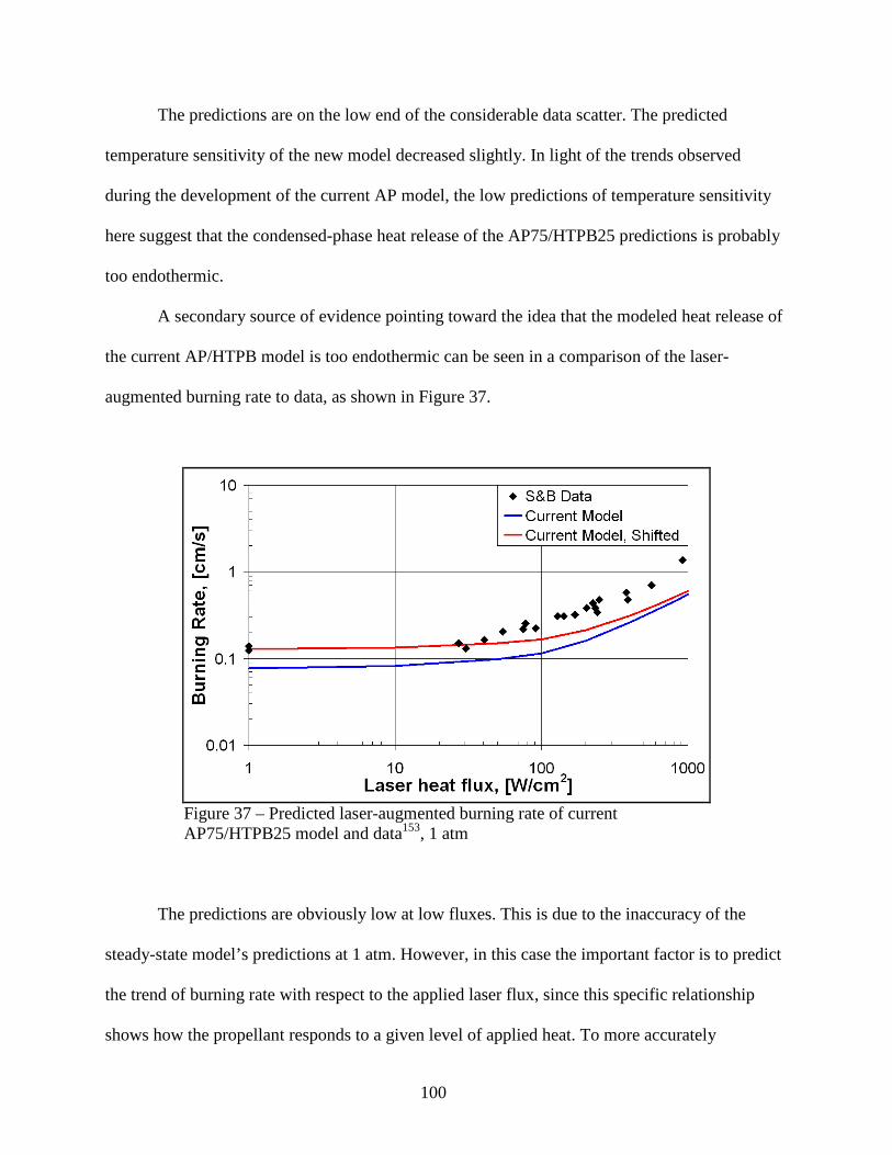
100
The predictions are on the low end of the considerable data scatter. The predicted
temperature sensitivity of the new model decreased slightly. In light of the trends observed
during the development of the current AP model, the low predictions of temperature sensitivity
here suggest that the condensed-phase heat release of the AP75/HTPB25 predictions is probably
too endothermic.
A secondary source of evidence pointing toward the idea that the modeled heat release of
the current AP/HTPB model is too endothermic can be seen in a comparison of the laser-
augmented burning rate to data, as shown in Figure 37.
Figure 37 – Predicted laser-augmented burning rate of current AP75/HTPB25 model and data153, 1 atm
The predictions are obviously low at low fluxes. This is due to the inaccuracy of the
steady-state model’s predictions at 1 atm. However, in this case the important factor is to predict
the trend of burning rate with respect to the applied laser flux, since this specific relationship
shows how the propellant responds to a given level of applied heat. To more accurately

101
determine the ability of the current AP/HTPB model in this regard, a second line that is labeled
as “Shifted” is also shown in Figure 37, where a value of 0.052 cm/s (~40%) has been added to
the burning rate at 1 atm to account for the inaccuracy of the base prediction. In this case, the
slope of the graph is too shallow by a good margin, falling short on average by ~75% above a
laser heat flux of 100 W/cm2 and implying that the calculated condensed-phase heat release is
too endothermic.
The melt layer predictions of AP75/HTPB25 (defined in the current AP/HTPB model as
the distance between the location of the melt temperature, 735 K, and the surface) are reasonable,
lying in the range of 1 to 1.5 microns between pressures of 10 and 1000 psi. No data were found
for comparison. Predicted surface temperatures are low when compared to the propellant data of
Powling139 and Bakhman141, as presented in Figure 38.
Figure 38 – Predicted surface temperature of current and Tanner AP75/HTPB25 models and data139,141
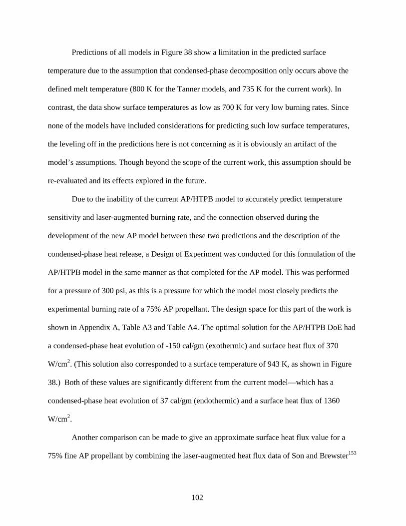
102
Predictions of all models in Figure 38 show a limitation in the predicted surface
temperature due to the assumption that condensed-phase decomposition only occurs above the
defined melt temperature (800 K for the Tanner models, and 735 K for the current work). In
contrast, the data show surface temperatures as low as 700 K for very low burning rates. Since
none of the models have included considerations for predicting such low surface temperatures,
the leveling off in the predictions here is not concerning as it is obviously an artifact of the
model’s assumptions. Though beyond the scope of the current work, this assumption should be
re-evaluated and its effects explored in the future.
Due to the inability of the current AP/HTPB model to accurately predict temperature
sensitivity and laser-augmented burning rate, and the connection observed during the
development of the new AP model between these two predictions and the description of the
condensed-phase heat release, a Design of Experiment was conducted for this formulation of the
AP/HTPB model in the same manner as that completed for the AP model. This was performed
for a pressure of 300 psi, as this is a pressure for which the model most closely predicts the
experimental burning rate of a 75% AP propellant. The design space for this part of the work is
shown in Appendix A, Table A3 and Table A4. The optimal solution for the AP/HTPB DoE had
a condensed-phase heat evolution of -150 cal/gm (exothermic) and surface heat flux of 370
W/cm2. (This solution also corresponded to a surface temperature of 943 K, as shown in Figure
38.) Both of these values are significantly different from the current model—which has a
condensed-phase heat evolution of 37 cal/gm (endothermic) and a surface heat flux of 1360
W/cm2.
Another comparison can be made to give an approximate surface heat flux value for a
75% fine AP propellant by combining the laser-augmented heat flux data of Son and Brewster153
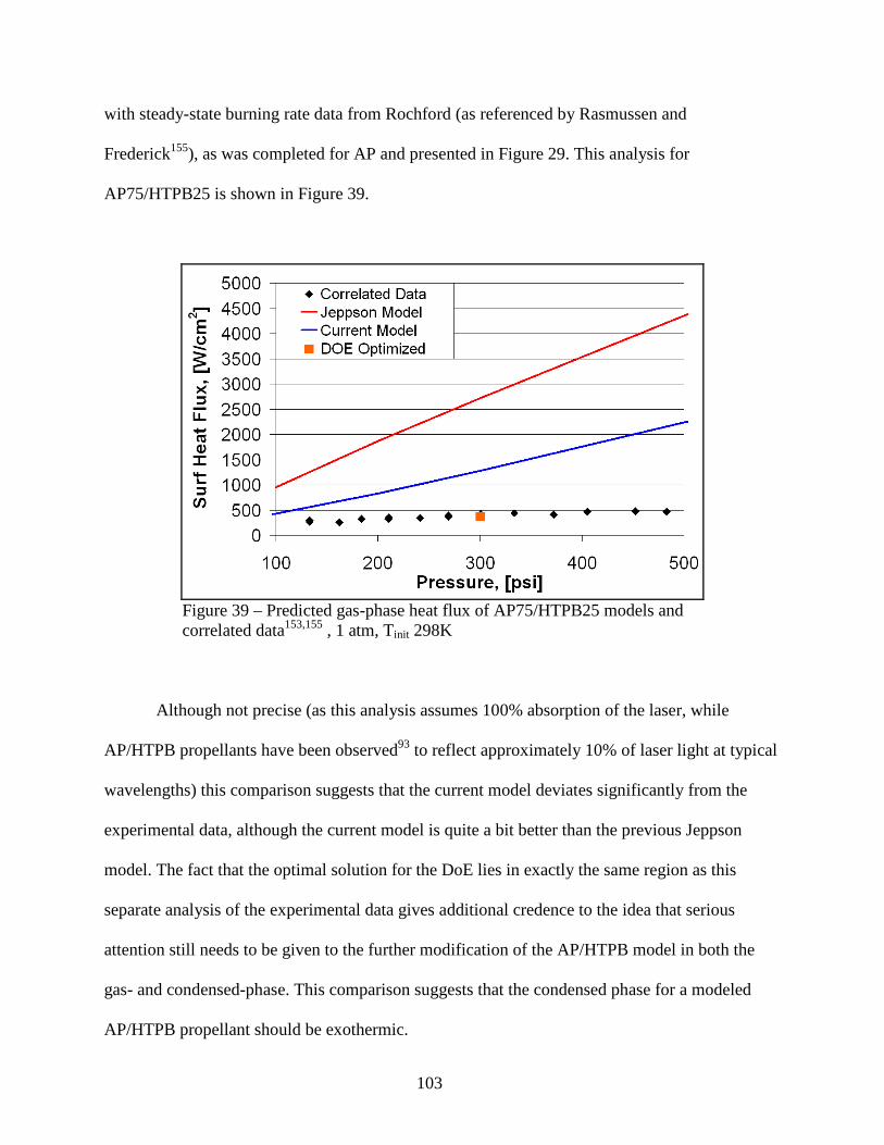
103
with steady-state burning rate data from Rochford (as referenced by Rasmussen and
Frederick155), as was completed for AP and presented in Figure 29. This analysis for
AP75/HTPB25 is shown in Figure 39.
Figure 39 – Predicted gas-phase heat flux of AP75/HTPB25 models and correlated data153,155 , 1 atm, Tinit 298K
Although not precise (as this analysis assumes 100% absorption of the laser, while
AP/HTPB propellants have been observed93 to reflect approximately 10% of laser light at typical
wavelengths) this comparison suggests that the current model deviates significantly from the
experimental data, although the current model is quite a bit better than the previous Jeppson
model. The fact that the optimal solution for the DoE lies in exactly the same region as this
separate analysis of the experimental data gives additional credence to the idea that serious
attention still needs to be given to the further modification of the AP/HTPB model in both the
gas- and condensed-phase. This comparison suggests that the condensed phase for a modeled
AP/HTPB propellant should be exothermic.

104
4.4.2 AP/HTPB MODEL: 80% AP, 20% HTPB
A comparison of the predicted burning rate for AP80/HTPB20 to both the Tanner
predictions and experimental data63,156,157 Figure 40 is given in .
Figure 40 – Predicted burning rate of current and Tanner AP80/HTPB20 models and data63,156,157, Tinit 298K
The predictions are good at moderate pressures, falling within the scatter of the data. The
trend at moderate pressures also looks much better than that for AP75/HTPB25. Although the
Cohen-Nir data at high pressure (and large AP particle size) probably weren’t burning under
premixed conditions, the data were included here because of their extension to low pressure,
where the premixed assumption of the current model more likely holds. As with AP75/HTPB25,
the predictions at low pressure (15 psi) are still considerably different than the data suggest
(~45% too low).
Calculated temperature sensitivity of AP80/HTPB20 is also much lower than the
experimental data157-159, as presented in Figure 41.
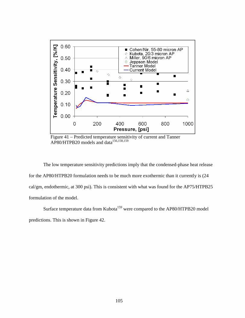
105
Figure 41 – Predicted temperature sensitivity of current and Tanner AP80/HTPB20 models and data156,158,159
The low temperature sensitivity predictions imply that the condensed-phase heat release
for the AP80/HTPB20 formulation needs to be much more exothermic than it currently is (24
cal/gm, endothermic, at 300 psi). This is consistent with what was found for the AP75/HTPB25
formulation of the model.
Surface temperature data from Kubota159 were compared to the AP80/HTPB20 model
predictions. This is shown in Figure 42.
106
Figure 42 – Predicted surface temperature of current and Tanner AP80/HTPB20 models and data159, Tinit 298K
The model predicts these data fairly well (within 50 K) though high, but is still low as
compared to the Powling139 data presented in Figure 38. Predicted surface temperatures should
probably be slightly higher than experimental data, which are collected as bulk measurements
averaged over the entire propellant surface, while the defined surface temperature of the model is
a point defined by a remaining liquid fraction of 0.0001%. Given the fact that the current
propellant model already needs to be changed significantly to more accurately describe an
AP/HTPB propellant, the level of accuracy of the model for this formulation was deemed
acceptable.
4.4.3 AP/HTPB MODEL: 84% AP, 16% HTPB
There were relatively few sources of experimental validation found for this formulation
of an AP/HTPB propellant. The first comparison was given in the extrapolations of Figure 34,
107
though this apparent validation relies completely on the observed trends of AP/HTPB propellants
formulated with a smaller fraction of AP. The same trends are present for the AP84/HTPB16
formulation of the model that were observed in the predictions of the other two proposed
formulations: a fair amount of accuracy at 6.8 and 20.4 atm, while over-predicting the system at
high pressure, and under-predicting at low pressure.
Korobeinichev et al.160
Figure 43
report data for an 84% AP CTPB-propellant at a pressure of 0.08
atm as shown in .
Figure 43 – Predicted burning rate of current AP84/HTPB16 model and data160, Tinit 298K
The single data point at 0.08 atm (1.17 psi) is more than an order of magnitude larger
than that predicted by the model. There are effectively two ways to make the predicted burning
rate higher in a propellant/ingredient model. Either the gas-phase heat flux at the surface
(currently, ~15 W/cm2) or the exothermicity of the condensed phase (currently, ~30 cal/gm,
exothermic) needs to be increased. The predicted gas-phase heat flux near of the surface of the

108
propellant can be compared to the gas-phase data of Korobeinichev et al.160. A comparison of
their data to both the Jeppson model and the current AP/HTPB model for this formulation is
given in Figure 44.
Figure 44 – Predicted temperature profile of current and Jeppson AP84/HTPB16 models and data160, 0.08 atm, Tinit 298K
The predicted temperature rise near the surface is in excellent agreement with the data.
Thus, the possibility of affecting a change upon the surface heat flux through the gas-phase
mechanism to increase the predicted burning rate of the propellant seems like the wrong choice.
The second option is to increase the exothermicity of the condensed phase, an option that is
consistent with what has been seen for the other two formulations of the AP/HTPB model.
4.4.4 SUMMARY
The current steady-state AP/HTPB model predicts a few experimental data sets, but falls
short in describing several others, most noticeably those necessary for proper validation. Burning

109
rate, final species, and final flame temperatures are accurate. It is desired that the model should
be able to predict laser-augmented burning rate, temperature sensitivity, and surface temperature
as well. A minimal set of changes was made to Tanner’s original model so that it could be
applied toward ignition simulations, which resulted in the model predicting a more consistent
melt layer thickness. Current results suggest that the condensed-phase decomposition of the
AP/HTPB model needs to be exothermic instead of endothermic, with a much smaller amount of
heat being released in the gas-phase flame. Such a change will require a very large effort,
including both the condensed-phase decomposition scheme and gas-phase mechanism as well.
The application of the current AP/HTPB model to the ignition code will include the steady-state
modeling assumption that no condensed-phase decomposition occurs below a melting
temperature of 735 K.
The work completed for the AP/HTPB model that has been presented in Chapter 4.4 is
shown in Figure 45 within the validation structure first presented in Chapter 3.
Figure 45 – Validation structure including work on the current AP/HTPB model

110
4.5 HMX IGNITION
After having made so many changes and improvements to the ignition code, it was
important that the HMX model be re-validated against the ignition data of HMX, for which the
ignition code was originally developed to predict. A localized comparison of the improved
ignition code results, Meredith’s original results, and HMX ignition data95 is given in Figure 46.
It is encouraging to see that the changes made to the ignition code to allow for the
modeling of other propellant ingredients, and to make its calculations more consistent with the
assumptions in the Phase3 code, have only affected HMX ignition predictions slightly.
Figure 46 – Predicted time to ignition of current and Meredith HMX models and data95, 1 atm, Tinit 298K
4.6 SUMMARY OF FOUNDATIONAL WORK
It was important that each of the propellant/ingredient models that form the foundation of
the final predictions (AP/HTPB/Al cookoff) be validated against as much pertinent data as
possible. Additionally, it was important to make sure that the codes emplying those models were

111
verified to a point such that we could have confidence in their predictions. The two
propellant/ingredient codes, Phase3 and the ignition code, were verified and then improved to be
able to apply the propellant/ingredient models that formed the core of this work. HMX
predictions from the new ignition code compared well to previous calculations made by the
original ignition code and still compared well to the data. The updated AP and AP/HTPB steady-
state models have been validated against the data and seem to be performing well.
The work presented in this chapter has formed a foundation for the next application of the
steady-state models: the ignition code and making predictions for laser-driven ignition events.

112

113
Few things are harder to put up with than the annoyance of a good example.
-- Mark Twain
CHAPTER 5: IGNITION
After validating the steady-state propellant/ingredient models using Phase3, they were
next applied to the ignition code for the purpose of predicting the transient response of a
propellant/ingredient to an external source of heat. It is an important concept that the previous
validation of these steady-state models, which has been presented in Chapter 4 for AP
monopropellant and several formulations of an AP/HTPB propellant, can only allow for the
correct prediction of the final condition of a laser ignition prediction: laser-augmented steady
state. In the development of a steady-state model, the heat evolution predictions of the condensed
and gas phases can contain a wide range of variability. In like manner, it is possible that a wide
range of validated steady-state models, each with variously defined chemical-kinetic reaction
schemes in the condensed and gas phases, can accurately predict laser-augmented burning rates.
Ultimately, it is up to the developer to decide when the accuracy of a model is “good enough”
with respect to both steady-state and transient ignition predictions and when more work needs to
be accomplished.
Ignition results for the current work will be presented in this chapter from the AP model,
the AP/HTPB model, and the AP/HTPB/Al model via the application of heat by CO2 laser.
Predictions of time to a surface temperature of 513 K for the AP/HTPB and AP/HTPB/Al
models are presented along with the ignition results, since condensed-phase decomposition has
been seen to affect these propellants at sub-melt temperatures. Cookoff predictions for the
114
AP/HTPB/Al model are also presented, along with comparisons to available data. Additionally,
an effort to further validate the steady-state models, or suggest direction for further research
based upon the results of the current ignition work, will be made.
5.1 AP IGNITION
Predicted ignition results for AP in the current work are presented as time to melt
temperature, which is assumed to be equal to the time to first decomposition or a surface
temperature of 735 K. The connection between the melt temperature and first decomposition is
consistent with the assumptions made in Phase3 as part of the current steady-state model. This
connection between melt temperature and first decomposition is also consistent with the
observations of Atwood65 for the ignition of AP. It is assumed that reactions occurring within the
gas and condensed phases subsequent to reaching the melting condition begin sufficiently fast
after this point to allow the propellant ingredient to transition to self-sustaining combustion after
removal of the laser flux over a period of time on the order of several milliseconds. As such,
ignition predictions for AP are functions only of the thermal conductivity, melting temperature,
and as will be shown, the absorptive properties of the crystal with regard to laser light.
Two initial ignition simulations were completed using the original Gross AP model to
ascertain the effects of using a penetrating/absorbing laser versus applying the laser heat only as
a boundary condition. (Prior to this work, HMX ignition predictions only included application of
the laser heat as a boundary condition at the solid/gas surface interface.) The results of this sub-
study for the current AP model compared to data65 in Table 16. The value of “Log-Slope”
presented in Table 16 is the slope of a straight line passing through the data/predictions on a log-
log plot. This value is used to determine how well the predictions fit the trend of the data in this
115
region. For all ignition predictions presented here and later, the laser heat flux is approximated as
a near-square wave with a rise time of 0.2 ms161
Table 16 – Initial ignition predictions using the Gross
and is assumed to be composed of
monochromatic light.
17 AP model
Ignition, 34 atm Laser Flux Time to Ign Log-Slope [cal/cm2/s] [ms] [--]
Atwood Data (2007) 50 61.95 -1.41 100 23.28
Abs/Pen Laser (239 cm-1) 50 89.16 -1.46 100 32.32
B.C. Laser 50 41.36 -1.97 100 10.58
Since the Gross model was never used for ignition calculations, the large difference
between the data and predictions is unsurprising. The reason for making this comparison was
only to determine the best way to apply the heat of the laser for ignition simulations. (Predictions
made by the current model showed similar results in regard to the desired trend since all thermal
parameters between the two models are similar and no condensed-phase decomposition is
accounted for during these simulations.) As presented, the Log-Slope of the predictions when
applying the laser heat as a boundary condition is too steep by 35%, whereas that for the
absorbing/penetrating laser is within 4%. This result is consistent with the observation144 that AP
crystals are fairly transparent to the wavelength of laser light typically used, as previously
mentioned in Chapter 4. The absorption parameter of AP, as measured by Isbell and Brewster144,
is on the order of 102 cm-1, rather than 103 cm-1 like most other propellants/ingredients. As such,
it was decided to include the penetrating/absorbing laser sub-model for all AP, AP/HTPB, and
AP/HTPB/Al ignition predictions made in the current work.

116
5.1.1 RESULTS AND DISCUSSION
Intial results for AP ignition using the current model are compared to experimental
data65,87 in Figure 47.
Figure 47 – Initial AP ignition predictions using current model and data65,87, 34 atm
Although the ignition predictions for AP at an initial temperature of 298 K are high
(simulations taking too long to heat up), the slope of the predictions is very similar to the data.
Two primary factors in predicting time to ignition are the thermal conductivity and melt
temperature (or initial decomposition). AP is fairly unique in that neither an accurate melt
temperature nor thermal conductivity (for temperatures above 513 K) has been well-defined by
experimental observation. In an effort to find possible reasons for the long prediction times of the
model, a parametric sub-study was conducted using the current model in Phase3 to define a
relationship between melting temperature and the thermal conductivity of solid AP that could be

117
used to explore the possible prediction space of the ignition calculations. This was accomplished
by comparing the cubic-phase-thickness predictions of the current AP steady-state model to the
data of Beckstead and Hightower140. The following assumptions were made to accomplish this:
1) sub-melt decomposition (below 735 K) is insignificant;
2) the thermal conductivity of orthorhombic AP is equal to that measured by Parr123;
3) the thermal conductivity of cubic and melted AP are equal at the melt temperature and have the same trend with temperature, a trend observed by Osman162
4) the trend of thermal conductivity with respect to temperature for AP is equal to that measured by Parr
for perchlorate salts—although the thermal conductivity may change to a reasonable degree at the cubic transition temperature of 513 K;
123 for all temperatures within the model. Using the current steady-state AP model and the above assumptions, a relationship
between the A-parameter of Parr’s thermal conductivity fit for temperatures of interest (A+B∙T)
and the melt temperature of the solid was constructed by matching the steady-state burning rate
of the propellant through the following iterative procedure:
1) define the melt temperature of AP in the model (ranged from 620 K to 870 K);
2) define the thermal conductivity of cubic-phase and melted AP (A-parameter);
3) vary the condensed-phase pre-exp to predict burning rate163
4) compare the predicted cubic-layer thickness to the B&H
accurately;
140 data;
5) if the predicted cubic-layer thickness was different than the data, return to step 2;
6) if the predicted cubic-layer thickness was accurate, record both values (melt temperature and A-parameter);
7) return to Step 1 until the entire range of melt temperatures is populated.

118
Through this method, Equation 28 was derived, which is a fit of the necessary A-
parameter of Parr’s thermal conductivity fit for a proposed melt temperature, Tm, that will fit the
AP cubic-phase thickness of Beckstead and Hightower140.
( ) 3112742 1089.6107.1104.11008.4 mmmmParr TTTTA ⋅⋅−⋅⋅+⋅⋅−⋅= −−−− (28)
This correlation was then used to make a variety of ignition predictions toward
determining the combination of melt temperature and thermal conductivity that would result in
accurate ignition predictions for AP, while using the temperature-insensitive laser-absorption
parameter suggested by Isbell and Brewster144 of 239 cm-1. This process resulted in an optimized
melt temperature of 657 K and an A-parameter for the cubic- and melt-phase thermal
conductivity of 1.906∙10-3 to predict the available time to ignition data.
There are a couple of troubling things about these results.
1) a melt temperature of 657 K for AP is considerably lower than what has been historically suggested by other research;
2) the optimized A-parameter suggests that the thermal conductivity of the cubic-phase is 25% higher than that of the orthorhombic phase, which seems like a large difference;
If the above assumptions are valid, the final results are still dependent upon the accuracy
of the laser-absorption parameter and its insensitivity to temperature. Isbell and Brewster’s144
laser-absorption data for AP has a significant amount of variation around the laser wavelength of
10.6 microns, as shown in Figure 48. It has been reported164
that this local variance is due to the
breathing frequency of the perchlorate ion being close to this wavelength of radiation. This
concept is similar to that of the breathing frequency of water being close to the wavelength of
radiation used within a microwave oven.

119
Figure 48 – Laser-absorption parameter data144 for AP, 1 atm, 298K
An additional calculation was completed to find the value of absorption parameter for
temperatures above 513K needed to correctly predict the data using the thermal conductivity and
melting temperature of the current AP model. This optimized value was 405 cm-1, a value not too
different than the datapresented by Isbell and Brewster144. Ignition predictions using these
revised parameters for AP and pertinent experimental data65,87 are shown in Figure 49. These
predictions were made using the absorption parameter value suggested by Isbell and Brewster for
orthorhombic AP (239 cm-1), and the optimized value (405 cm-1) for all temperatures above the
cubic-phase transition temperature of 513 K.

120
Figure 49 – AP Ignition results using current mode and data65,87, 34 atm
The validity of these optimized calculations rides on the idea that the effective absorption
parameter of the AP crystal varies with respect to temperature. One concept that suggests the
absorption of the laser by AP should be a function of temperature is that the electrical
conductivity of the solid, which directly impacts the absorptivity of other materials to radiation,
varies with respect to temperature. It is well-documented that AP is electrically conductive165-167
in the range of 300 to 600 K (increasing conductivity with increasing temperature) and also at the
burning surface168
99
during steady-state deflagration. It is unknown how this property of AP, or its
variance with temperature, might affect the effective absorption parameter, which has only been
measured at 298 K.
It is also interesting to look at how ignition predictions evolve as a function of time. A
time track of the predicted burning rate, surface temperature, and maximum gas-phase
temperature versus simulation time for AP ignition is shown in Figure 50.

121
Figure 50 – AP ignition predictions for current model, transients of burning rate surface temperature and flame temperature
Oscillations such as these that occur just after the point of ignition within a model, occur
because of the difference between the state of the condensed-phase solution at steady state and
that at the point of ignition. At the point of ignition, the modeled surface of the
propellant/ingredient will have a void fraction that is very small (only a small portion of the
material will have decomposed); at steady-state the void fraction at the surface will be very low
(identically zero, but assumed to be 0.0001%) . As the rate of condensed-phase decomposition is
dependent only upon temperature, the large amount of material present near the surface results in
an initially large rate of decomposition to be predicted.
The first feature in Figure 50 that is immediately apparent—while keeping in mind the
similar plot for HMX in Figure 10—is the sharpness of the burning rate curve at the point of
ignition. At a surface temperature of 735 K, the condensed-phase decomposition reactions begin
and spike rapidly. This effect is due to the assumptions of the AP model concerning the initiation
of sub-melt decomposition and ignition time being equal to time to melt temperature. The

122
ignition code’s improved ability to transition from inert heating to decomposing solid over a very
small time scale is evident here. After the initial spike, the model transitions to augmented,
steady-state burning quickly. For the current AP model, this oscillatory transition time varied
from 2 to 20 ms for heat fluxes in the same range as the collected data.
The second interesting feature of Figure 50 is the overshoot of the predictions for burning
rate and maximum gas-phase temperature. This phenomenon is consistent with the behavior of
other ignition models that include an exothermic condensed phase. Upon initial inspection, the
overall endothermic decomposition of the current AP model probably shouldn’t produce such an
effect. However, the first 30% of all decomposition that occurs in the current AP model is
assumed to be exothermic. The decomposition rate during this time is calculated as if 100% of
the AP present will eventually decompose along the exothermic path, and so the calculations
only see the exothermic portion of decomposition during this time. The overshoot observed here
is consistent with both the model’s assumptions and the presented calculations of previous
predictions made by the ignition code (Figure 10).
In fact, this initial exothermic decomposition is probably too exothermic, as evidenced by
the very large overshoot in the initial burning rate. This could possibly be remedied by proposing
an initial condensed-phase decomposition step that is more consistent with species seen during
partial decomposition. If such a step were taken, the model would then have to be altered to
contain a bubble-phase reaction to occur sub-surface between the decomposition products of the
new initial exothermic reaction and the sublimation products of the currently proposed
endothermic decomposition step, to predict surface species that are consistent with observed
data33. This type of setup is consistent with that used by the Beckstead et al.44 AP model. The
current work, however, has only taken into account the accurate prediction of the surface species

123
data and has not made any changes to the steady-state model to more accurately predict
conditions specific to ignition.
The third interesting feature in Figure 50 that should be noted is the relaxation to, and
final values of, laser-augmented steady-state burning rate. Unfortunately, the ignition simulation
results have final gas-phase predictions that were quite different from what was expected, with
predicted final flame temperatures being too high and predicted burning rates too low when
compared to predicted results from Phase3. A grid-refinement study was completed for ignition
cases involving a 100 cal/cm2/s heat flux to see what effect, if any, refining the grid would have
upon these predictions. The spacing of grid points in the gas phase of the ignition code was
uniform in all cases presented for the current work, unless otherwise specified. Figure 51
presents the final flame temperature and laser-augmented burning rate predictions of the AP
model in the ignition code as it depends on the gas-phase grid.
Figure 51 – AP ignition code verification, gas-phase grid-refinement study, 34 atm, 100 cal/cm2/s

124
Values used for comparison in Figure 51 (final flame temperature and laser-augmented
burning rate) were calculated using the Phase3 code. These predictions should be identical to the
final values calculated by the ignition code after all of the transients have died out. Predicted
values from the ignition code were close to those calculated by Phase3. Using a gas-phase grid
that is sufficiently refined (less than 1 micron grid resolution according to the trends of Figure
51) resulted in the ignition code correctly predicting both laser-augmented burning rate and final
flame temperature accurately.
Arguably, the most important section of the grid to have the proper refinement is near the
solid surface, as this is where the steepest gradients are present for the physical processes of the
model. Refining the grid sufficiently at the surface, however, was seen to not be the sole
problem as an additional grid refinement study, which used a grid that was fine near the solid
surface and progressively larger out into the far-field, failed to show any significant degree of
improvement. This result may be due to the fact that the discretization of the gas-phase equations
is currently implemented in the ignition code only for uniform grids, and that as a given
discretization becomes more non-uniform more error will be present in the solution.
In general, using a grid with a high level of refinement was prohibitive due to the very
small time step that had to be employed to keep the convective-CFL number (u∙Δt/Δx) below 1,
for numerical stability. Simulations completed that used a uniform gas-phase grid with a spacing
of 5 microns (the grid size used for all simulations in the current work, unless otherwise
specified) already necessarily dropped down to timesteps on the order of five nanoseconds
during the ignition transient for an AP simulation. Making further reductions became
increasingly expensive with regard to overall wall-clock time. It is good that the code is
exhibiting trends that are consistent with making correct final predictions.

125
Although no data could be found in the literature for time to ignition for AP with respect
to pressure, calculations were made to determine if the model’s results were consistent with what
would be expected. Predicted times to ignition (surface temperature of 735 K) varied by less than
5% for pressures of 1 to 34 atm. This very minimal amount of variation for time to ignition
versus pressure is consistent with the fact that no sub-melt decomposition is present in the
current model and thus there is no thermal effect of decompostion prior to ignition. Therefore,
the only mode of variation in predicted time to ignition is the effect of thermal diffusivity on the
surrounding atmosphere as it conductively cools the surface. The trend with respect to pressure is
correct in this regard, with simulations at higher pressure taking slightly longer to reach the
ignition (melting) temperature for a given level of laser heat flux, since the effect of gas density
at higher pressures will lead to more heat being conducted away from the surface of the
propellant/ingredient.
As currently presented, the calculated predictions of the current AP model do not include
the time corresponding to the most interesting part of the ignition process: the transition to
steady state. This transition encompasses the region of time in which an ignited propellant
ingredient will or will not be able to transition to steady-state burning. The ability of a heated
propellant/ingredient to transition to steady-state burning has historically been viewed as being
dependent upon the amount and location of energy stored within the condensed and solid phases.
This is determined by the temperature profiles within the condensed and solid phases at the time
the heat flux is removed. High heat fluxes applied to the propellant/ingredient result in a steeper
temperature gradient. Steeper temperature gradients result in a smaller portion of the propellant
being at a raised temperature and thus reactive state. When the laser heat is removed, if there
isn’t enough propellant/ingredient that is sufficiently reactive due to raised temperatures, then the

126
reactive portion of the propellant/ingredient will burn away and the gas-phase flame will blow
out.
A comparison of the predicted temperature profiles for the current AP model at steady
state and those at the predicted ignition times for several levels of laser heat flux is given in
Figure 52. Times at which the ignition results were taken are significantly different from one
another, but correspond to each simulation reaching a surface temperature of 735 K.
Figure 52 – Predicted temperature profiles of current AP model, 34 atm
It is interesting to note that experimental data confirm that each of the three lower heat
flux cases presented in Figure 52 should transition to steady-state burning, and that each of the
predicted condensed-phase temperature profiles at ignition is significantly shallower than the
profile prediction at steady state. This suggests that there should be enough predicted energy
within the propellant ingredient for a transition to steady-state burning to occur once the laser
heat source is removed. These results corroborate the concept typically used to describe this

127
condition in reality that AP samples will tend to transition to steady-state burning for conditions
included these levels of heat flux. Based on the trend of the results in Figure 52, a significantly
higher laser heat flux would be necessary for AP to have an experimental go/no-go time that
diverges from the time of inert heating (as previously described in Figure 8). Indeed, it wasn’t
until the modeled laser heat flux was higher than 1000 cal/cm2/s that the ignition code predicted
a condensed-phase temperature profile for AP that even approached the steepness of that
predicted by the steady-state model.
There are three main factors that can also be considered as important when determining
the go/no-go point of actual propellants/ingredients from the perspective of the gas phase:
1) the ability of the kinetics to respond quickly enough to the loss of thermal input and avoid blowing out the near-surface flame;
2) the time over which the laser flux is removed;
3) the relative amount of laser heat being applied to the propellant/ingredient under augmented conditions versus those at unaugmented conditions.
Upon initial inspection, the first factor is possibly beyond experimental control. If,
however, such a determination were able to be made, it would very likely come about by
investigating the effect of pressure on go/no-go times. At higher pressures, the kinetic rate of
gas-phase reactions would be higher, and thus they would be able to respond to a given change in
applied heat more quickly and thus be more resistant to being blown out. This factor would
evidence itself as shorter go/no-go times for identical levels of heat flux at higher pressures,
which is consistent with what has been observed66 for composite propellants in the past.
Although, this concept probably has some cross-over effects with the second factor: the gas-
phase heat flux near the surface of the propellant/ingredient.
The second parameter of primary importance to the ability of a propellant/ingredient to
transition to steady-state burning after a laser-driven ignition event is the difference between the

128
heat flux at the surface of the propellant/ingredient under laser-augmented conditions (including
the laser flux) versus those at un-augmented steady state. For instance, it would be easier for a
propellant/ingredient with a steady-state heat flux of 800 cal/cm2/s (at a given pressure) to
transition to steady-state burning after the removal of a 200 cal/cm2/s heat flux (laser heat is
~20% of the total), than it would be for a propellant/ingredient with a steady-state heat flux of
100 cal/cm2/s to transition to steady-state burning after the removal of the same laser heat flux
(laser heat is ~67% of the total) if the heat is ramped off over the same period of time. Knyazeva
and Zarko79,80 reported that if a propellant/ingredient is exposed to a heat flux of greater than
37% of its steady-state surface heat flux at a given pressure, then the propellant/ingredient
combustion would become unstable and would extinguish. This result, however pertinent, is
dependent upon both the accuracy of the combustion model that they used and the rate at which
the heat flux was removed. A longer removal time for the laser would allow for a greater heat
flux to be applied to the propellant/ingredient model while still allowing for the predictions to
transition to steady state burning regardless of how large the flux level was.
The third factor affecting the ability of a propellant/ingredient to transition to steady-state
burning after a laser-driven ignition event is a straight-forward concept: any propellant/
ingredient exposed to any level of laser heat flux should be able to transition to steady-state
burning if the laser heat flux is removed at a slow-enough rate and the propellant/ingredient will
deflagrate at the pressure of the experiment. It is unclear how varying the ramp-off time of the
laser might affect go/no-go data that has previously been collected. Vilyunov and Zarko67 have
reported that typical HMX propellants at 10 atm with a laser heat flux of 20 cal/cm2/s will
transition to steady state if the laser is ramped off over more than 3 milliseconds, but
extinguishes if the ramp-off time is less than 1 ms. No application of this study, however, could

129
be found for AP/HTPB propellants. It would be very interesting to see new research
accomplished to explore the effects on ignition data of varying the laser ramp-off time and what
we might be able to infer from those relationships when comparing them to applicable
propellant/ingredient models.
It has already been shown how times to ignition can be affected by treating the laser heat
flux as a boundary condition applied at the surface of the propellant/ingredient versus applying
the penetration/absorption parameters from literature99 in a Beer’s law sub-model, which is how
it is handled in the current code. The predicted results when using these two methods are
different at laser-augmented steady-state conditions. The ignition code was used to determine
this for an AP case with a laser heat flux of 100 cal/cm2/s. The burning rates for the two cases
were nearly identical (less than 2% difference in final values), but the predicted surface
temperature for the penetrating/absorbing laser was 40 K higher than that for the boundary-
condition laser case. These results are consistent with what is expected. Burning rate is
determined by the amount of heat supplied to the surface of the propellant/ingredient. The
amount of heat is identical in both cases. A laser applied at the boundary condition implies a
higher heat flux at the surface of the propellant/ingredient, which for an approximately constant
value of thermal conductivity, necessitates a steeper temperature profile and thus higher
predicted surface temperature.
5.1.2 FURTHER ATTEMPTS TO VALIDATE THE STEADY-STATE MODEL
In an effort to explore the AP steady-state model to its fullest extent, the ignition results
were examined to see if they might elucidate something more that might be applied to its further
development. Six sub-studies were completed to determine an optimal melt temperature for AP

130
at six separate levels of solid-phase absorption parameter by using Equation 28 and the process
earlier described for determining the optimal melting temperature or laser absorption parameter.
These results, optimized to accurately predict the time to ignition of AP at a laser flux level of
100 cal/cm2/s, showed that varying the absorption parameter continuously between 190 and
750 cm-1 corresponded to optimized melt temperatures ranging from 635 to 898 K. This range of
melt temperatures encompassed the entire range of values that have, to our knowledge, been
previously proposed for AP. A list of these three correlated input parameters for the current AP
model at six separate levels of the continuous range is presented in Table 17.
Table 17 – Possible inputs for current AP model LaserAbsParam MeltTemp A-param, λ
[cm-1] [K] [cal/cm/s/K] 190 635 2.076∙10-3 340 705 1.645∙10-3 425 745 1.515∙10-3 590 822 1.388∙10-3 750 898 1.266∙10-3
This range of absorption parameter corresponds to a variance in the laser-light
wavelength according to Isbell and Brewster144 from 10.6000 microns to 10.6167 microns; a
window of less than 0.16%. The predictions of the current models assume monochromatic light,
which is possibly not the case in reality. If the CO2 laser-light wavelength is assumed to be
exactly 10.6 microns, then the above analysis implies an AP melt temperature of 635 K, which
again seems low when compared to historically suggested values, and a thermal conductivity
increase at the 513 K interface of 37%, which also seems quite high. Additionally, these
predictions were made for a simulation where 100% of the laser is absorbed by the solid. The
solution for a system where a portion of the laser is reflected away, however, which is probably

131
more consistent with reality, would result in a yet lower necessary melt temperature and
correspondingly higher thermal conductivity shift at the cubic-phase transition temperature.
Predicted times to ignition for AP at 34 atm using two separate levels of absorption
parameter (one with a modeled melt temperature of 657 K and the other for the current model)
are shown in Figure 53 along with data from Atwood et al.65,87 Predictions and data are both
reported as time to first-decomposition, which is equivalent to time to melt temperature for
model predictions. It is important to note that the results presented in Figure 53 constitute
separate models with significantly different inputs and do not only represent the simple variation
of the laser absorption parameter for AP.
Figure 53 – Predicted times to ignition for two variations of the current AP model and data65,87, 34 atm
Predictions compare favorably to the data. Three things in particular are noted about the
predictions of the two trial models presented:
132
1) the predicted difference between the two trial models is very small;
2) the predicted difference decreases as initial temperature increases;
3) the predictions begin to diverge noticeably from one another at higher heat fluxes. This result suggests that the melt temperature, thermal conductivity of the cubic and melt
phases, and laser absorption parameter might be inferred by extending predictions and data to a
higher heat flux. Extending the predictions to 3000 cal/cm2/s, however, (the maximum heat flux
level applied to a sample of AP128 that could be found by a literature search) only resulted in a
20% difference between predicted results, with actual times to ignition being sub-millisecond. It
seems likely that such an extension to the experimental data, if completed, would probably fall
within the scatter of the data and also make the rise time of the laser161 a significant portion of
the prediction time, thus negating the ability to infer anything of value.
There is also a suggestion in Figure 53 that AP ignition data taken for samples at initial
temperatures lower than 298 K might be able to tell us something more since the predictions
between the two presented models (with defined melt temperatures of 657 K and 735 K) are
further apart for those with an intial temperature of 298 K than 373 K. This suggestion is
somewhat counterintuitive, in that heat has historically been added to AP when collecting
experimental data, but given the results of the current model another sub-study was completed in
this vein. The results, however, showed relatively little difference (less than 15% between
models with defined melt temperatures of 657 and 898 K) for calculations made using an in
initial temperature of 225 K. This sub-study did show, however, that the predicted LogSlopes of
the various trial models with an initial temperature of 298 K had a range of values from -1.63 for
the 898 K melt temperature model to -1.48 for the 657 K melt temperature model. This result
again suggested that, if the model’s assumptions are correct, then the actual melting temperature
of AP might be in the lower portion of the range included in Table 17, as Atwood et al.65

133
reported the LogSlope of their collected data with an initial temperature of 298 K to be -1.41. It
would be most elucidating, however, to have additional ignition data for AP over a wider range
of heat fluxes, as that currently available does not seem to be able to provide more specific
conclusions by comparison to the current AP model.
5.1.3 SUMMARY
Time to ignition data for the current AP model have been presented and compare quite
well to experimental data (± 10%). Since no experimental data report accurate melting
temperature or thermal conductivity (above 513 K) for AP, a range of possible model inputs
(thermal conductivity, melting temperature, and laser absorption parameter) has been presented
that allow for the accurate prediction of time to ignition. The current model uses a set of inputs
that includes a melting temperature of 735 K. Transient results of the ignition model are
consistent in behavior with previous calculations made for HMX using the ignition code. Ignition
data used for comparative validation of the model span a very small range. More ignition data for
AP with respect to levels of heat flux would be helpful for future development.
The work completed for the AP ignition model that has been presented in Chapter 5.1 is
shown in Figure 54 within the validation structure first presented in Chapter 3.
134
Figure 54 – Validation structure including work on the current AP ignition model
5.2 AP/HTPB IGNITION
While improving the AP/HTPB ignition model, a large focus was placed upon the
validation of the individual components that formed the complete model. Input parameters for
the AP/HTPB model include those for AP that have been used in the current AP steady-state
model, which have been validated against available experimental data in Chapter 4. They also
include those for HTPB that have been used in previous AP/HTPB models7,62 at BYU and/or
taken from recent experimental measurement. Additionally, it was important that the same
assumptions be used in the steady-state and ignition codes so that predicted results from the the
AP/HTPB model could be compared to one another directly.
One concept of the ignition model that must be addressed before any results are presented
includes the current assumptions regarding condensed-phase decomposition within the model.
The Phase3 steady-state propellant code employs the assumption that condensed-phase
decomposition begins at the melt temperature of the modeled ingredient/propellant. This value is
typically measured for a single propellant ingredient (like monopropellant nitramines, for which
135
the code was originally developed) but becomes somewhat arbitrary when considering a model
for propellants that contain multiple ingredients with various melt temperatures. When modeling
propellants such as AP/HTPB that have evidenced significant decomposition89,90,139,169
65
at
temperatures lower than the temperature defined in the current AP/HTPB model (735 K) and that
have also been seen to begin decomposing very early-on in relation to the go/no-go point in
ignition work , using the assumption that no sub-melt decomposition is present at sub-melt
tempearatures may negatively affect the modeled results.
Despite experimental observations to the contrary, the results for the current AP/HTPB
ignition model have been treated in like manner to the AP ignition model, wherein time to
ignition is reported as time to heat the surface of the propellant to the assumed melt temperature
of 735 K. This choice is consistent with the assumption made in the current steady-state
AP/HTPB model. This defined surface temperature condition is also in the same region as
ignition temperatures that have been reported as being used in industry170 (700-750 K) and by
Eager et al.171
The primary reason for making the decision neglect sub-melt decomposition within the
current AP/HTPB ignition model was due to convergence issues within the ignition code when
using the AP/HTPB gas-phase mechanism with Tanner’s HCN-elimination reaction. Inclusion of
this reaction in the gas-phase mechanism led to near-immediate divergence of all calculations
attempted (for ignition and cookoff) within the ignition code, while not including it allowed for
simulations to be completed without issue. Thus, the HCN-elimination reaction was removed
from the gas-phase mechanism for all simulations made by the current model. Removing the
HCN-elimination reaction from the AP/HTPB steady-state model resulted in a drop of the
predicted burning rate by 50%. All calculations that have been made using the current AP/HTPB
(833 K) for propellants of similar formulation.

136
model for times that predicted significant condensed-phase decomposition had low burning rates
due to this issue. Thus, any possibility of making valid predictions using a model that used sub-
melt decomposition were lost, as well as any confidence in the simulated region of time after the
point of ignition. Thus no transient predictions or transitions to steady-state augmented burning
seem credible or will be discussed in the results of the AP/HTPB ignition model. These
predictions should be considered by future efforts, after the short-comings of the current
AP/HTPB model have been rectified. Predictions presented from the current work only include
simulation times when the predicted burning rate of the propellant/ingredient is assumed to be
near zero.
5.2.1 RESULTS AND DISCUSSION
There are three metrics available in reported experimental data for validating any ignition
model: time to first decomposition, time to ignition (first light, somewhat arbitrary), and go/no-
go time. Time to first decomposition has been assumed to be at a surface temperature of 513 K,
time to ignition at a surface temperature of 735 K, and go/no-go times are not predicted.
Time to first decomposition was reported by Atwood et al.65 and determined by an
observable, physical change in the surface of the propellant. Model predictions for a time to
surface temperature of 513 K have also been made, since the cubic phase transition has been
suggested172
65
as the approximate temperature at which significant reaction in the AP/HTPB
condensed phase begins to occur. Predictions of time to ignition (735 K, solid lines) and time to
assumed first decomposition (513 K, dashed lines) for AP80/HTPB20 and AP84/HTPB16, along
with corresponding data from Atwood et al. ,88, are presented in Figure 55.

137
Figure 55 – Data65,88 and near identical predicted times to ignition for two formulations of the current AP/HTPB model, 1 atm
The difference between the predictions for these two formulations of the AP/HTPB
model is very small and may be occurring because no sub-melt decomposition has been
accounted for in the current ignition model. The only affected difference between the two is a
very small change in the effective thermal conductivity of the modeled propellants due to
formulation. It is immediately obvious that the model predictions have slopes that are steeper
than the go/no-go data and more shallow than the first-decomposition data. There are several
possible reasons for these differences in regard to the model.
Parameters of greatest impact on AP/HTPB time to first decomposition predictions are
the thermal conductivity and laser-absorption parameter of the solids. The temperature range in
which these calculations are made (298 to 513 K) contain the most accurate and repeatable
measurements of thermodynamic properties for AP (data varies by ±11% around the thermal
conductivity fit) and HTPB (data varies by ±40% around the thermal conductivity fit). The
current codes use a volume-averaged, linear-interpolation method to calculate the overall
138
propellant thermal conductivity for the AP/HTPB model. The analysis presented previously in
Section 4.3.3 on steady-state modeling of AP/HTPB propellants suggests that the thermal
diffusivity of the AP/HTPB model was being described accurately, but that the application of
Parr’s fits in the model were possibly over-estimating the thermal conductivity to some small
degree.
The amount of variability present for AP absorption of the laser was presented in Figure
48, and includes a possible range of values that could feasibly work within the construct of the
AP model (Table 17) and thus be applied to the AP/HTPB model. There is significantly less
variability in the absorption parameter of HTPB, which has been observed144 to have a value of
361 cm-1, varying by less than 3% over the range of laser-light wavelength to which AP has been
applied in the current model.
Any variance in the amount of applied laser energy that is absorbed by the solid
propellant has not been considered by the model. It has been reported145 that 15% of the laser
applied to HMX during laser-augmented combustion is lost due to reflectivity and/or attenuation
due to absorbing gas-phase species and liquid droplets above the surface. The reduction of the
apparent laser energy absorbed by the surface of a propellant/ingredient has been reported173
There is also one factor concerning the experimental data that should be addressed.
Atwood et al.
for
AP (7.5%) and AP-based propellants (10%).
88 brushed ZrC powder onto the surface of the propellant to “enhance the
absorption” of the applied laser energy for ignition data. They stated that this coating made the
absorptivity of the heat source (CO2 laser or arc-image) more uniform. It is unknown how the
application of this powder, and/or its uniformity on the surface, might have affected the way the
laser was absorbed, the way/amount in which the laser might have been reflected, or the level to

139
which it might have affected the heating rate of the propellant surface due to direct heating of the
powder by the laser. Additionally, the chemical kinetics at the propellant surface might have also
been affected since ZrC has been reported174
Ignition predictions for the current AP/HTPB model are compared against a wider range
of AP/HTPB ignition data
elsewhere to be a catalyst for AP-based propellants.
None of these possibilities has been taken into account in the current model.
65,87,91-94,116,175,176 Figure 56 in . Note that some of the data have been
designated as first-light (FL), which signifies the initiation of significant gas-phase reaction and
is assumed to be approximately equal to (but just longer than) the time of first decomposition.
Figure 56 – Predicted time to ignition and time to first light for current AP/HTPB model and data65,87,91-94,116,175,176, 1 atm
The AP/HTPB ignition data are bounded by the predictions of a time to surface
temperature of 513 K and 735 K. Predictions are quite good at lower fluxes but begin to under-
predict time to ignition at high heat fluxes. The predictions based on a time to surface
temperature of 735 K are very close to the recent first-light data of Cain and Brewster, which

140
data are similar to the assumptions made in the model (CO2 laser, first light reported, and fine
AP particles—2 micron—used in the propellant), though these data are fairly different than the
other sets in the graph. Some of the data sets presented contain propellants with small fractions
of carbon, iron oxide, or nitramines, and include vaious sources of heat supply (conduction by
hot gases, ARC-image lamps).
Predictions reported in Figure 56 will shift slightly upward if laser reflection is taken into
account (predicted time to temperature will become longer) An AP/HTPB model with a
condensed-phase heat release that is exothermic, as has been suggested by the current work,
would lead to predicted ignition times that were shorter, if sub-melt decomposition were
included. An approximate effect of applying an quasi-exothermic, sub-melt decomposition and
data65,87,91-94,116,175,176 is shown in Figure 57.
Figure 57 – Effect of sub-melt decomposition on current AP/HTPB model and data65,87,91-94,116,175,176, 1 atm

141
The exothermic approximation made for these results was accomplished by changing the
heats of formation for AP and HTPB to result in a condensed-phase heat relase of ~150 cal/gm,
exothermic. Two levels of condensed-phase decomposition (pre-exponential values of 107 and
109) were investigated within the temperature range over which AP is assumed to be in the cubic
phase by the current model (513 to 735 K). These two values represent a case where
decomoposition over this temperature range is three orders of magnitude less than that of the
melt layer (more consistent with observations119 for RDX, upon which the Phase3 code was
based) and another where the decomposition is only a single order of maginitude less than that in
the melt layer (more consistent with an assumption of continuous condensed-phase kinetics).
The case with a pre-exponential of AP/HTPB decomposition of 109 was the only one at which a
significant difference between the predictions was noticable within the range of applicable heat
fluxes, and thus only predictions made for this level of decomposition have been reported in
Figure 57. Although the overall effect is not large, this graph does show that the effect of sub-
melt decomposition becomes more pronounced at lower heat flux levels and would become even
more prominent for the lower heat fluxes associated with cookoff.
A majority of the ignition data presented for AP/HTPB are at the go/no-go point of the
propellant sample, which is very ill-defined for making such determination within the model.
Experimental go/no-go data are reported as the time at which 50% of the samples attempted will
transition to steady-state burning once the heat source is removed. Such a comparison, were it to
be made by prediction, would call for an extremely precise description of the reactions and
kinetics within the propellant model, which the current AP/HTPB steady-state model does not
have.
142
In reality, the ability of an AP/HTPB propellant to be able to transition to steady-state
burning after the removal of the heat flux is likely dependent upon the amount of heat held by the
propellant as compared to that under steady-state burning conditions. This comparison can be
made by looking at the predicted temperature profile within the solid propellant at the time of
ignition and that for the predicted propellant at steady state. Ignition temperature profiles that are
steeper than those at steady state will more than likely extinguish, while those that are more
shallow should be able to transition to steady-state burning. This comparison for AP80/HTPB20
is given in Figure 58.
Figure 58 – Predicted temperature profiles of current AP80/HTPB20 model, 1 atm
In the above figure, the case for 50 cal/cm2/sec looks to be reasonably close to the
temperature profile prediced at steady state, though it is difficult to say as the temperature profile
of the steady-state model is extremely steep near the surface. The profiles will of course be
143
altered for a condensed-phase model that includes exothermic decomposition occurring earlier
than the melt temperature. An exothermic decomposition would not only shorten the time to
ignition but will also have the propensity to widen the thermal layer of the propellant that is at a
raised temperature due to the fact that heat is being generated at points within the sub-surface by
decomposition.
The largest and possibly most important factor relating to the accuracy of go/no-go
predictions is an accurate portrayal of evolved/absorbed heat associated with condensed-phase
decomposition. Reactions in the condensed phase lead to the evolution of gas-phase species,
which in turn react in a gas-phase flame. Propellant ingredients such as AP, which appear to have
an endothermic condensed-phase decomposition, should then be dependent upon the heating and
subsequent ignition of the evolved gas-phase species before being able to reach a go/no-go
condition. In contrast, AP/HTPB propellants appear to have an exothermic condensed-phase
decomposition and might be able to reach a condition whereupon the reactions in the condensed
phase could thermally run away and lead to the go/no-go condition before an actual gas-phase
ignition event occurs.
5.2.2 SUMMARY
The current AP/HTPB model describes ignition data across a wide range of fluxes,
bounding the data for time to surface temperature of 513 K (assumed first decomposition) and
735 K (assumed ignition), but were unable to predict the trends of go/no-go times. Go/no-go
predictions are much more difficult to predict as they require a very accurate representataion of
the kinetics and heat release associated with the deflagration of the propellant/ingredient.
Predictions from the current AP/HTPB and model are based upon the current Phase3 assumption
144
that no sub-melt decomposition occurs prior to ignition. This assumption should be relaxed in
the future, allowing the kinetic decomposition of the condensed phase to determine ignition
times, instead of simply the predicted temperature of the propellant surface.
The work completed for the AP/HTPB ignition model that has been presented in Chapter
5.2 is shown in Figure 59 within the validation structure first presented in Chapter 3.
Figure 59 – Validation structure including work on the current AP/HTPB ignition model
5.3 AP/HTPB/AL IGNITION AND COOKOFF
After the AP/HTPB model was validated against experimental data for steady-state and
ignition conditions, it was applied toward defining the AP/HTPB/Al model. The kinetic
decomposition scheme for the AP84/HTPB16 formulation of the AP/HTPB model was used to
describe the condensed-phase kinetics of the AP/HTPB/Al model, since the ratio of AP to HTPB
in that formulation is very similar to a typical aluminized propellant. As with the AP84/HTPB16
formulation of the AP/HTPB model, there has been no consideration of multi-modal
distributions of AP that would be necessary to make realistic propellants with this formulation.

145
Although non-realistic, this is consistent with the idea that there is no affect of multi-modal
distributions upon the physical properties of the propellant built into either model, and that the
current predictions of the model are for times prior to those when multi-model distributions of
AP might make an effect upon ignition predictions. Looking into the necessary multi-modal
distributions of AP and their further effect upon simulations was beyond the scope of the current
work.
The only difference in the calculations of the AP/HTPB and AP/HTPB/Al models is the
inclusion of inert aluminum in the AP/HTPB/Al model. There is no current consideration of
aluminum in the gas phase or for kinetic reactions involving aluminum in either phase of the
current model. Additionally, the aluminum reflection model detailed in section 4.2 was
employed for the AP/HTPB/Al model simulations in all presented ignition calculations. Laser
heat lost due to reflection according to the sub-model varies linearly from 0 to 37% for
aluminum backscatter values ranging from 0 to 100% within the reflection sub-model. This
range is dictated by the absorption of laser light as it passes through the modeled components of
an AP/HTPB propellant. Assumptions used for that sub-model are that 0% of the incident laser
light is absorbed by the aluminum particles, 14% is back-scattered, and the remaining 86% is
forward-scattered. These parameters within the reflection sub-model led to 6% of the incident
laser heat being lost due to reflection. The current assumption for the AP/HTPB/Al ignition
model is that time to ignition is equal to the time the surface takes to reach a temperature of
735 K, which is consistent with the assumptions made for the AP/HTPB steady-state model.
146
Predicted times to ignition for the AP/HTPB/Al model are compared to experimental
data
5.3.1 IGNITION RESULTS AND DISCUSSION
,115,175
There are two groups of data presented in
in Figure 60.
Figure 60, nearly all of which are bound by the
first-decomposition and ignition predictions of the model. The first group is from a number of
different sources (designated by **: Atwood Ign, Baer, Lengelle, and China Lake) that were all
referenced by Wilson et al. for their work with an AP/PBAN/Al propellant.
Figure 60 – Predicted time to ignition and time to first light for current AP/HTPB/Al model and data65,115,175, 1 atm
None of these external data sets were reported with references, formulations, or
experimental conditions; however, this group of data was compared to the experimental cookoff
data collected by them. The formulation of their propellant was reported as being an 80% solids
loading of AP and aluminum in a PBAN binder, without specificity for either component;
however, all of their figures referred to “NASA production samples”, which for the space shuttle

147
propellant are typically closer in formulation to 86% solids loading (AP and aluminum) in a
PBAN binder. In this case, the most important parameter is the loading of aluminum, since it will
contribute the greatest effect upon the overall thermal conductivity of the propellant.
When comparing this first group of referenced data and the Zanotti and Galfetti175 data to
the most recent Atwood et al.65 data, it looks as if all the experimental data points excluding the
Atwood set are more consistent with first-light times rather than go/no-go times. The current
formulation of the AP/HTPB/Al model is most consistent with the propellant used for the go/no-
go data set from Atwood et al.65 for an AP/HTPB/Al propellant with 68% AP and 20%
aluminum (overall 88% solids loading), although the predictions of the model are furthest from
it.
The trend of the ignition predictions in Figure 60 looks fairly good when compared to all
of the data, but the go/no-go data from Atwood et al.65 obviously occur at significantly longer
times than those predicted by the model at these levels of heat flux (by 2 to 20 times). In this heat
flux range, the large difference between data and model predictions is similar to that from the
AP/HTPB model, upon which the AP/HTPB/Al model is based, and is determined by the amount
of time necessary for the chemistry within the condensed-phase decomposition to develop to a
point such that it can transition to steady-state burning when the heat is removed. This larger
difference for the AP/HTPB/Al model is also due to the extra time needed for the propellant to
absorb the necessary amount of near-surface heat to reach the point of ignition. Heat collects less
efficiently at the surface for aluminized propellants because more heat is reflected away from the
propellant due to the aluminum particles, and heat is also conducted more quickly into the bulk
of the propellant, due to the higher thermal conductivity.
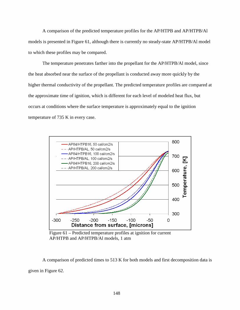
148
A comparison of the predicted temperature profiles for the AP/HTPB and AP/HTPB/Al
models is presented in Figure 61, although there is currently no steady-state AP/HTPB/Al model
to which these profiles may be compared.
The temperature penetrates farther into the propellant for the AP/HTPB/Al model, since
the heat absorbed near the surface of the propellant is conducted away more quickly by the
higher thermal conductivity of the propellant. The predicted temperature profiles are compared at
the approximate time of ignition, which is different for each level of modeled heat flux, but
occurs at conditions where the surface temperature is approximately equal to the ignition
temperature of 735 K in every case.
Figure 61 – Predicted temperature profiles at ignition for current AP/HTPB and AP/HTPB/Al models, 1 atm
A comparison of predicted times to 513 K for both models and first decomposition data is
given in Figure 62.

149
Figure 62 – Aluminum effects on current model of predicted time to first decomposition and data65, 1 atm
The predictions are quite similar to the data. If the assumptions of the current model are
valid, then it seems as if the AP/HTPB contribution to the thermal conductivity of the modeled
propellant might be too high due to the too-shallow slope of both predictions. This is consistent
with what was seen in the AP/HTPB model. The contribution of aluminum to the thermal
conductivity may also be too low, since the difference between the two predictions is smaller
than the spread in the data. Although, this possibility is difficult to determine because the
difference between the preidictions of the two models is probably due to both the increased
thermal conductivity and increased laser light reflection of the aluminized propellant. These two
trends in the predictions (slope too steep and difference between predictions for aluminized and
non-aluminized propellants) are consistent with what was presented in Figure 32, which
compared the thermal conductivity data from similarly formulated propellants to the
approximations used within the current models.

150
A comparison of predicted times to ignition for the AP/HTPB model and experimental
go/no-go points65 is quite different, as shown in Figure 63.
It is unclear exactly why there is such a large difference between this specific data set
(Atwood65, go/no-go) and the various others that were presented in Figure 60. The difference
between the AP/HTPB and AP/HTPB/Al predictions and the corresponding data is quite large,
not only in value but also in slope. Arguably, the majority of the difference between the
AP/HTPB/Al predictions and data can be attributed to the same cause of the difference between
the AP/HTPB model and data: the additional time required by the propellant’s decomposition
chemistry to reach a point at which the transition to steady-state combustion may be attained.
Figure 63 – Aluminum effects on current model of predicted time to ignition and data65, 1 atm
Another portion of this larger difference between the AP/HTPB/Al predictions and data
might come from the amount of time it takes the propellant to come to an augmented burning
rate, which is affected by the higher thermal conductivity of the aluminized propellant. Also,

151
prior to entering the gas-phase, aluminum acts primarily as a heat sink, and thus the need for
additional energy within the condensed-phase, and thus additional time is required for the
modeled propellant to be heated by the laser. The amount of aluminum that is uncovered as the
solid AP/HTPB propellant begins to decompose is also possibly playing a significant role.
Aluminum particles present near the surface during this span of time (between the first
decomposition of the propellant and the go/no-go time) may have the chance to agglomerate,
ignite, lift into the gas-phase domain, and increasingly scatter the laser light before it ever
reaches the surface of the propellant, if time scales are sufficient. All of these possible effects
will tend to increase the amount of time it takes for a modeled propellant to reach a go/no-go
condition as it inhibits the amount of heat that is applied to the surface of the propellant.
The variation of predicted time to ignition for given levels of defined backscatter within
the aluminum reflection sub-model is shown in Figure 64 with go/no-go data65.
Figure 64 – Aluminum reflection parameter variance within AP/HTPB/Al model and go/no-go data65

152
The predictions for the current model assume that 14% of the laser light incident upon the
aluminum particles will be back-scattered, while the remaining 86% will be forward-scattered.
The resultant spread of the predictions ranges between 60% and 120% across this range of heat
flux. The results at low heat fluxes for the maximum amount of back-scatter from the aluminum
particles nearly makes up the entire difference between the predictions and the data; however, it
is unlikely that the laser light back-scatters so perfectly (100%) from the aluminum particles,
since the dominant scattering angle at these particles sizes is near forward.
Mie scattering calculations show a cross-sectional increase of the aluminum particles
(over their geometric cross section) by approximately a factor of 2, varying slightly with the size
of the particle. When including these effects, the predicted times to ignition become an additional
10% longer. Although this is an important effect to consider for the reflection sub-model, the
laser-driven ignition predictions and experimental go/no-go times are still fairly far from one
another at these relatively high levels of heat flux. The difficulty in using comparisons such as
these for validation is that the aluminum reflection model becomes a very important parameter
for making ignition predictions of an AP/HTPB/Al propellant (resulting in predictions varying
by a total of 70 to 130%), but doesn’t affect cookoff predictions at all. In essence, without some
sort of separate validation, the reflection sub-model becomes a tuning parameter for ignition
predictions and doesn’t add anything of value to understanding or predicting cookoff. Earlier
validation of the AP/HTPB/Al model to ignition data in Figure 60 is thus the primary source of
validation for this level of the model.
The work completed for the AP/HTPB/Al ignition model that has been presented in
Chapter 5.3.1 is shown in Figure 65 within the validation structure first presented in Chapter 3.

153
Figure 65 – Validation structure including work on the current AP/HTPB/Al ignition model
5.3.2 COOKOFF RESULTS AND DISCUSSION
Cookoff systems typically include a sample of propellant or high explosive material that
has been confined within a given container. This container, and the enclosed propellant, are
heated by an external source (fire, oven, electric blanket) until an ignition event occurs. These
events can range from being relatively small (fast cookoff, high heat flux) where only a small
portion of the propellant is heated before the point of ignition, to explosively large (slow
cookoff, low heat flux) where a majority of the propellant is heated to a reactive temperature
before ignition.
The results from AP/HTPB/Al cookoff model were surprising on the whole and yet very
consistent with what had been seen during the prior validation of the propellant/ingredient
models. A comparison of the experimental data and model predictions for three different cookoff
scenarios is given in Figure 66 along with data114-116.
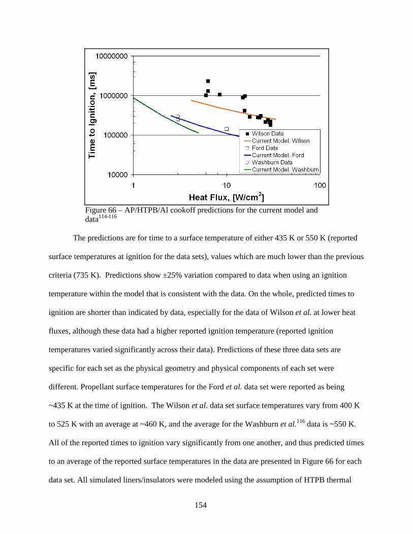
154
Figure 66 – AP/HTPB/Al cookoff predictions for the current model and data114-116
The predictions are for time to a surface temperature of either 435 K or 550 K (reported
surface temperatures at ignition for the data sets), values which are much lower than the previous
criteria (735 K). Predictions show ±25% variation compared to data when using an ignition
temperature within the model that is consistent with the data. On the whole, predicted times to
ignition are shorter than indicated by data, especially for the data of Wilson et al. at lower heat
fluxes, although these data had a higher reported ignition temperature (reported ignition
temperatures varied significantly across their data). Predictions of these three data sets are
specific for each set as the physical geometry and physical components of each set were
different. Propellant surface temperatures for the Ford et al. data set were reported as being
~435 K at the time of ignition. The Wilson et al. data set surface temperatures vary from 400 K
to 525 K with an average at ~460 K, and the average for the Washburn et al.116 data is ~550 K.
All of the reported times to ignition vary significantly from one another, and thus predicted times
to an average of the reported surface temperatures in the data are presented in Figure 66 for each
data set. All simulated liners/insulators were modeled using the assumption of HTPB thermal

155
properties, assuming no decomposition, due to a lack of pertinent data on the various materials
used in the experimental works.
The current AP/HTPB/Al model is based on the kinetic decomposition scheme of the
AP84/HTPB16 formulation of the AP/HTPB model, which is assumed to reach “ignition” when
the surface of the propellant has reached 735 K. The simulated propellant has no condensed-
phase decomposition prior to this temperature. This assumption was made both to keep the
propellant ignition models consistent with the steady-state models and to allow for convergence
of the ignition code. Two of the experimental data sets for cookoff reported the ignition event to
occur once the propellant surface had reached a temperature of ~435 K. This observation is
consistent with what has been observed in the past by others114,177
116
for cookoff systems that
included insulators and liners. The more recent findings of Washburn et al. have shown
ignition temperatures in the realm of ~550 K for a cookoff system that only included the
propellant and steel casing, which is more consistent with surface temperatures associated with
the bare ignition data of AP/HTPB propellants47,178
Temperatures at the inner steel surface of the cookoff system reported by Wilson et al.
.
115
and a comparison of the predicted propellant surface temperatures of the current model to data
are given in Figure 67.
It is likely that the reported low surface temperatures at ignition of Wilson et al.115 are
due to the thermal expansion of the steel container/article and opening of an air gap (added
resistance to heat flow) between the propellant/liner/insulator and the steel case. The size of the
air gap has been reported by Meredith and Beckstead3 as being a significant variable for
predicting time to ignition for cookoff systems. The size of any air gaps in the referenced
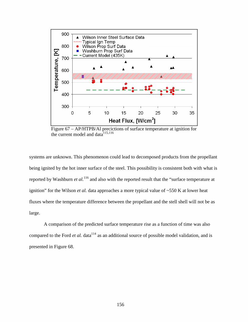
156
Figure 67 – AP/HTPB/Al precictions of surface temperature at ignition for the current model and data115,116
systems are unknown. This phenomenon could lead to decomposed products from the propellant
being ignited by the hot inner surface of the steel. This possibility is consistent both with what is
reported by Washburn et al.116 and also with the reported result that the “surface temperature at
ignition” for the Wilson et al. data approaches a more typical value of ~550 K at lower heat
fluxes where the temperature difference between the propellant and the stell shell will not be as
large.
A comparison of the predicted surface temperature rise as a function of time was also
compared to the Ford et al. data114 as an additional source of possible model validation, and is
presented in Figure 68.

157
Figure 68 – Predicted surface temperature of an AP/HTPB/Al cookoff simulation for two boundary-condition types and data114, 10 W/cm2
Properties for the liner, insulator, and steel shell used in this calculation were those
presented by Ford et al., except for those of the actual propellant, which were calculated by the
current model. Propellant property differences between those reported (measured) by Ford et al.
and those used in the current model were within ±30% of each other across the temperature
range of interest (298 to 435 K). Three different simulations are presented in Figure 68 for
comparison: one base case and two variants. The first variant included a new application of the
external heat flux (convective versus constant heat flux) and the second variant included a
change in the size of the air gap between the propellant and liner. The thermal expansion of a
cylindrical steel shell was calculated to grow to ~0.3 mm prior to the ignition point by
completing a simple thermal analysis of the steel using a thermal expansion coefficient of
1.1∙105/K. The predicted temperature profile of the base case at ignition using the current model
was nearly identical to the modeling efforts reported by Ford et al.

158
The base case was run with a constant external heat flux of 10 W/cm2 with an air gap of
0.5 mm. Comparison to the data is quite good early on, but the predictions rise significantly
higher than the data at longer times. This indicated that something had probably changed within
the experimental system that has not been accounted for in the model. A convective boundary
condition was also applied to the model that included a convective gas temperature of 1570 K
and heat transfer coefficient of 80 W/m2/K, as reported by Ford et al. Using this boundary
condition curtailed the divergence of the predictions from the data somewhat but not nearly
enough. Reducing the length of the air gap to 0.1 mm changed the results significantly, and
although varying the size of the air gap in this direction probably makes the simulation more
consistent with the experimental setup, it moves the predictions even further from the data.
A compliation of the ignition data, cookoff data, and predictions of the current model for
AP/HTPB/Al propellants is given in Figure 69.
Figure 69 – AP/HTPB/Al ignition and cookoff predictions with data65,114-116,175, 1 atm
159
At first glance, such a discrepancy between the location/trends of the cookoff and ignition
data/predictions seems odd. The difference, however, is one that has been addressed before by
Meredith and Beckstead3. They reported that it is the heat flux that reaches the surface of the
propellant, and not the heat flux applied to the outer casing, that is the important parameter when
considering cookoff data. This interfacial heat flux can be altered significantly in cookoff
systems by a number of factors, including: the properties of the liner(s), the metal casing, the
external conditions, the properties of the propellant, the length of the air gap, and others. It is
difficult to compare ignition events for these two configurations (ignition and cookoff) because
ignition data typically use precise heat flux control (quick ramp, followed by an overwhelming
majority of the time being spent at a constant applied heat flux), whereas cookoff systems
typically deliver a heat flux to the surface of the propellant that varies significantly.
One way of comparing these two disparate kinds of predictions is to determine the total
energy absorbed by the propellant by the time of ignition. This is made by integrating the heat
flux at the surface of the propellant with respect to time. Calculations for the AP/HTPB/Al
ignition data and current model predictions for the cookoff cases are presented in Figure 70. As
the necessary data (heat flux at the propellant surface) were not reported with the cookoff data,
the current model has been used to predict the total energy flux applied to the surface of the
propellant for these data sets using as assumed air gap of 0.5 mm.
160
Figure 70 – Total energy applied to ignited propellants at time of ignition, calculated from data65,114-116,175 using current model
Figure 70 is a representation of the total energy flux received by the propellant at the time
of ignition. The data points above should all lie along a similar line if the relationship between
time to ignition and energy flux received by the propellant is similar; a difference in a given data
set suggests that something is affecting the time to ignition. Predictions calculated from the
simulation of the Washburn et al. data presented in Figure 70 are much closer to extrapolations
of the bare propellant ignition data than that of either Wilson et al. or Ford et al. These sets of
predictions seem to imply that the cookoff propellants are probably igniting early when
compared to the bare-surface ignition data. Assumptions concerning the liners/insulators within
the cookoff model for representing each set of data are also probably affecting the results.
Additionally, the size of the air gap between the propellant and the steel case, the location of the
air gap, the transient growth of the air gap, and the increasing pressure of the system, are also
probably important factors, but have not been included in the current analysis. The temperature

161
of the steel shell at the time of ignition should probably also be taken into account, since the
decomposed products of the propellant will be in close proximity to it and could be leading to the
apparently early ignition of these systems.
5.3.3 SUMMARY
AP/HTPB/Al ignition predicitions bound nearly all of the pertinent data between
predicted time to first decomposition/light (at 513 K) and predicted melt temperature (735 K).
The remaining differences between predictions and go/no-go times probably arise from the
description of the condensed-phase propellant decomposition kinetics not accurately predicting
the pre-ignition regime, and the increased time associated with the effect of adding aluminum to
the simulated propellant.
AP/HTPB/Al cookoff predictions are within ±25% of the data, typically being low
(early). Remaining sources of variability may include: liner/insulator properties, accuracy of
propellant properties, transient thermal expansion of the steel shell, and possible early ignition
due to the proximity of decomposed gases to the heated steel shell of cookoff test articles.
The work completed for the AP/HTPB/Al ignition model that has been presented in
Chapter 5.3.1 is shown in within the validation structure first presented in Chapter 3. The
completion of this structure, starting with the steady-state predictions for AP combustion and
moving upward to this final configuration with the full propellant, has allowed for the final
predictions to be made with confidence regardless of the very small amount of data available for
validation purposes.

162
Figure 71 – Validation structure including work on the current AP/HTPB/Al cookoff model
163
There are those who would misteach us that to stick in a rut is consistency and a virtue, and that to climb out of the rut is inconsistency and a vice.
-- Mark Twain
CHAPTER 6: SUMMARY AND CONCLUSIONS
A significant amount of work has been accomplished toward improving two propellant
simulation codes and then seeking to understand at a foundational level solid propellant/
ingredient models and their application toward steady-state and transient ignition predictions.
The current work has made it a considerable point of focus to verify and validate the propellant
codes and models, build upon the knowledge gained during that process, and then apply that
knowledge toward making predictions in which confidence could be justified. A summary of
each effort previously presented will be given here, along with a brief opinion of the current state
of the work and suggestions as to where future consideration should be given.
6.1 CODE IMPROVEMENT WORK
A significant number of improvements have been made to the Phase3 and ignition code,
which allowed consistent predictions to be completed for three new propellant/ingredient
models.
Phase3 was improved to allow for the inclusion of phase transitions within the calculated
portion of the condensed-phase. The option to apply a penetrating/absorbing heat source (for
CO2 laser applications) was also developed.
Improvements to the ignition code included:
1) replacing the Chemkin software libraries with Cantera libraries;

164
2) translating the condensed-phase code from Fortran to C, making integration with
Cantera and further code development cleaner; 3) fixing inconsistencies in the definition of variables passed between the main program
and both internal subroutines and external libraries; 4) verifying the correct application of external software libraries to the code; 5) updating the condensed-phase equations and assumptions to be consistent with
Phase3, and changing the convergence criteria to an absolute basis; 6) adding the ability to transition between defined condensed-phase ingredients,
allowing each to be described by separate kinetic regimes; 7) adding a robust ramping scheme to handle decomposition kinetics within the
condensed-phase for decomposition reactions that increase rapidly at a given start temperature;
8) generalizing the code to allow for multiple ingredients to be modeled, instead of just
HMX; 9) adding two sub-models to the code for the application of aluminum to modeled
propellants; 10) including a multiple-step algorithm for solving the condensed-phase equations to
minimize their time-impact upon the overall simulation. The work accomplished has made a significant impact upon not only the behavior of the
ignition code but upon necessary calculation time as well. The original code would typically
diverge for the first several timesteps and had severe problems dealing with restart cases for
cookoff simulations that included more than one processor. In addition to these two issues being
resolved by the above changes, the improved code runs ~25-30% faster, diverges considerably
less often, and has been updated to integrate with a macro-centric Excel spreadsheet that was
developed and improved in parallel to the ignition code to graphically visualize the results of a
given simulation.

165
The culmination of the work associated with code development has resulted in a robust,
transient, CFD code that has the ability to model multiple propellants/ingredients with detailed
gas-phase kinetic mechanisms, moving melt interfaces, and ingredient transitions for describing
various phases and/or kinetic regimes of a given propellant/ingredient. The code can be used to
model either enclosed or bare-face propellants and their response to an externally-applied heat
source. It has no reliance upon the acquisition of any external software licenses or costs to use.
As it currently stands, the ignition code still has a few limitations that should be
addressed by future work. Gas-phase mechanisms that result in steep temperature profiles near
the surface require a high level of mesh refinement, which has been seen to be time prohibitive
due to the very small time step necessary to keep accuracy. The solution of the gas-phase
equations does not currently support an accurate approximation of the conservation equations for
a non-uniform mesh. It was also observed while working with the ignition code that cases
containing more than about 100 gas-phase nodes had significant convergence issues. The largest
problem, however, dealt with the very large wall-clock time necessary to complete simulations
that included the AP/HTPB and AP/HTPB/Al models (three to five times longer), since the
number of species in the gas-phase mechanisms of those models was much higher than the single
ingredient models.
A potential solution to a number of these issues would be to apply an operator-splitting
method, which employs a hybrid implicit-explicit approach to solve the individual conservation
equations using schemes that are particularly well-suited to each. Techniques such as those
proposed by Najm et al.179,180, Singe and Pope181 and Pope and Ren182
1) Advance the convection, energy, and a portion of the continuity equations by a half time step according to an explicit, predictor-corrector method;
that are based on Strang
splitting methods use a solution process for transient problems similar to the following:
166
2) Advance the species and remaining portion of the continuity equations by a full time step according to a semi-implicit, stiff-equation solution method, or table lookup;
3) Advance the convection, energy, and the same portion (as in step 1) of the continuity equations by a second half step according to the explicit, predictor-corrector method.
Making use of these methods would reduce the computational time necessary for overall
solution by decreasing the time spent using the time-expensive, implicit, non-linear methods that
are currently employed by the code for all conservation equations. Applying new solution
techniques such as these to the ignition code were not of primary concern during the current
work and would have required a relatively large amount of effort, yet the need for such a future
improvement of the ignition code, based upon the results of the current work, seems to be
justified.
6.2 STEADY-STATE WORK
The steady-state models associated with the current work included those for AP as a
monopropellant and AP/HTPB propellant. Since the AP/HTPB/Al propellant model was based
exclusively upon the AP/HTPB model, it will not be treated separately here.
6.2.1 AP MODEL
Several significant improvements were made to the AP model, which included reverting
to an older gas-phase mechanism and employing a newly-developed condensed-phase
mechanism based on the experimental observations and measurements of several sources. The
new AP model describes burning rate (± 10%), temperature sensitivity (within data scatter),
surface temperature (within data scatter), and melt-layer thickness (within the observed range) at
pressures ranging from 300 to 1200 psi, and also laser-augmented burning rate (± 50% for all
data and ± 20% for the most recent data) over an applied heat flux range of 20 to 400 cal/cm2/s.

167
There was significant improvement over the results of the original AP model, which were quite
different from the data in regard to the predicted melt-layer thickness (-95%) and laser-
augmented burning rate (+100%), and additionally over the updated version of the Gross AP
model, which additionally predicted a temperature sensitivity much higher than the data (+90%).
Improving the AP model in this way has allowed for confidence to be gained in both the steady-
state description of the results and the application of the AP model to the ignition code.
There is still a shortage of experimental data to help fully describe the necessary inputs of
the steady-state AP model (melt temperature, thermal properties above 513 K, temperature
variance of laser-absorption parameter), and so several reasonable assumptions were made,
based upon experimental observations where possible. Additional experimental data that would
be most helpful toward accurately describing the AP model in the future include an accurate
melting temperature for crystalline AP and an accurate thermal conductivity for temperatures
above the solid-phase transition temperature of 513 K. Additionally, having an idea of how the
absorptivity of crystalline AP might change with temperature would be of primary benefit to
further model development.
Validation of the AP model completed as part of this work has resulted in a model that
predicts a much larger data set than previous models and can now be confidently applied to both
steady-state deflagration and transient ignition simulations.
6.2.2 AP/HTPB MODEL
Relatively few changes were made to the AP/HTPB model as a whole. The model was
extended to include the AP84/HTPB16 formulation by extrapolation of the decomposition
reactions from the AP75/HTPB25 and AP80/HTPB20 formulations of the AP/HTPB model. The

168
changes to the AP/HTPB model comprised focusing the condensed-phase description to a
singular decomposition pathway and then altering the condensed-phase kinetics to accurately
predict burning rate while still accurately predicting final species fractions and final flame
temperature. Burning rate predictions for the current AP/HTPB model are accurate (± 50%) over
a pressure range of 50 to 300 psi, being low for lower pressures and high for higher pressures.
Deviations at high pressure are probably due to diffusion-flame appearance, with which this
research was not focused, and those at low pressure are assumed to be a result of the highly-
endothermic condensed-phase decomposition used in the current model. These are both
characteristics of the model that have been carried over from the previous version. Surface
temperature predictions are at the low end of the data scatter. Predicted temperature sensitivity
and laser-augmented burning rate are fairly poor, with predictions showing both low values and
shallow trends for each. Both of these characteristics are also consistent with the previous model.
Comparison of model results to experimental data suggested that the condensed-phase heat
release should be exothermic for fine AP/HTPB propellants, which the model was developed to
predict. Based on the results of the current AP model work, developing an AP/HTPB model with
exothermic condensed-phase decomposition should be able to allow for the accurate prediction
of the data sets that the current model fails to predict: temperature sensitivity, laser-augmented
burning rate, and low-pressure steady-state burning rate.
6.3 IGNITION WORK
Once the steady-state models were validated against experimental data, or deemed to be
sufficiently accurate for the purposes of the current work, the numerical inputs for the steady-
state models were applied to a transient ignition code to predict propellant/ingredient times to

169
ignition over a wide range of heat fluxes. This process was accomplished for both the AP and
AP/HTPB models for laser-driven ignition events, and for the AP/HTPB/Al model for both laser-
driven ignition and cookoff events.
The current AP model performed very well when applied to the ignition code in
predicting times to ignition (± 10%). Attempts to further validate the steady-state model using
the ignition modeling results were inconclusive due to the limited range of AP ignition data.
Thus, a range of possible values for three input variables within the AP model (melting
temperature, thermal conductivity above 513 K, and laser absorption parameter above 513 K)
was developed such that each set could result in the near-identical description of both steady-
state and ignition data. This set of input variables will allow for the model to be compared to
additional AP ignition data, as they become available. The assumption made regarding negligible
sub-melt decomposition within the AP model is consistent with AP ignition at the relatively high
heat fluxes to which the predictions were compared.
The current AP/HTPB and AP/HTPB/Al models described ignition data across a wide
range of fluxes, bounding the data for time to surface temperature of 513 K (assumed first
decomposition) and 735 K (assumed ignition), but were unable to predict the trends of go/no-go
times. Go/no-go predictions, however, are much more difficult to predict as they require a very
accurate representataion of the kinetics and heat release associated with the deflagration of the
propellant/ingredient. Predictions from the current AP/HTPB and AP/HTPB/Al propellant
models are based upon the current Phase3 assumption that no sub-melt decomposition occurs
prior to ignition.
An aluminum reflection model was applied to the AP/HTPB/Al propellant ignition
predictions based on a uniform scatter of reflective aluminum particles and calculations made by

170
a Mie particle code. The accuracy of the aluminum reflective model is unknown. A more
rigorous solution of the radiative transfer equation, as it pertains to the solid-phase distribution of
aluminum particles throughout the semi-transparent solid, would allow for the current model to
be evaluated, although such an effort was beyond the scope of the current work. The accuracy of
applying the Maxwell approximation of determining the effective thermal conductivity of
AP/HTPB/Al propellants is unknown but deemed sufficient. Modeling results suggest that the
modeled thermal conductivity of an AP/HTPB/Al propellant is too low, with the contribution of
the AP/HTPB being slightly too high and the effect of added aluminum being too small.
Additional experimental and/or theoretical work toward understanding the impact of aluminum
on the thermal properties of propellants to which it has been added would be helpful.
6.4 COOKOFF WORK
The results of the current AP/HTPB/Al cookoff work were very enlightening. Cookoff
predictions of AP/HTPB/Al propellants were good, with comparisons being slightly lower than
comparable experimental data (± 25%). Reported experimental ignition events occurred with
surface temperatures that were significantly lower than the assumed melt temperature of the
current model (735 K), and thus occurred before any condensed-phase decomposition within the
model. This emphasized the need for a significant change to the current AP/HTPB and
AP/HTPB/Al models, and also to the prior way of thinking when dealing with models for
propellants/ingredients such as these. Assumptions used for one propellant/ingredient are usually
not valid when modeling another propellant/ingredient and must instead be defined for each. The
assumption used in Phase3 that there is no significant sub-melt decomposition within the solid-
phase, an idea verified by observations for nitramines like RDX and HMX, does not seem to be

171
valid for AP/HTPB propellants. The progress necessary for determining a more valid
AP/HTPB/Al model for cookoff seems to be dependent upon the primary need for a model that is
better at first describing the steady-state data for non-aluminized AP/HTPB propellants, before it
can be applied to ignition/cookoff simulations.

172

173
APPENDICES APPENDIX A
The tables below are populated with the five descriptors of the condensed-phase portion
of the propellant/ingredient models used in the current work for the Design of Experiment. Input
parameters for the sub-studies included:
1) Pre-exponential of the condensed-phase decomposition reaction
2) Value of heat release(-)/absorption(+) due to condensed-phase decomposition
3) Value of heat flux at the surface of the propellant
Parameter 2 was varied using a sublimation decomposition reaction for the condensed
phase (Equation 27), and then varying the heat of formation of AP and/or HTPB so that the
calculated heat of reaction at the melt temperature (in Mathcad) was equal to the value of
Parameter 2 in the table. This process resulted in calculated heats of reaction that were close but
not identical to the defined levels of heat release, as Mathcad only used a single temperature to
calculate this value while Phase3 calculations occur over a range of temperature between the
melt temperature and the surface temperature.
The values selected for the three input parameters were chosen after several inital DoE
studies. In these initial studies, optimal solutions converged to points that were at the upper range
of the inputs. After widening the input ranges several times and shifting them according to the
results of each case, an optimal range of input parameters was arrived upon. Those ranges are
presented in the tables below.
174
Predictions of the condensed-phase portion of the model used as optimization parameters
in the sub-study included:
1) steady-state burning rate,
2) temperature sensitivity,
for model predictions at 68 atm (1000 psi). Temperature sensitivity calculations were
made between initial temperatures of 298 K and 323 K using Equation 29:
12
1
2ln
TTr
r
p −
=σ (29)
(Note: the impact of the gas-phase chemistry on the surface heat flux at 323 K is not taken into
account for these calculations (only the condensed-phase portion of the model was used to make
the calculations). Although this difference is probably small, the analysis detailed here can only
be considered as approximate due to this fact.
Table A1 – Setup for Design of Experiment of current AP model Run CP PreExp CP dHrxn SurfHeatFlux BurnRate TempSens
1 2.51∙1010 120 400 0.13667 5.791∙10-4 2 5.00∙1010 -120 5000 3.25285 1.227∙10-3 3 2.51∙1010 120 2700 0.84852 6.127∙10-4 4 1.00∙108 360 5000 0.79203 4.695∙10-3 5 1.00∙108 -120 5000 2.09567 7.644∙10-4 6 2.51∙1010 120 5000 1.52050 5.800∙10-4 7 1.00∙108 120 2700 0.70786 4.798∙10-4 8 2.51∙1010 -120 2700 1.81264 1.262∙10-3 9 2.51∙1010 360 2700 0.55695 4.069∙10-4
10 5.00∙1010 120 2700 0.86276 6.287∙10-4 11 5.00∙1010 360 400 0.08770 2.589∙10-4 12 5.00∙1010 360 5000 1.02249 3.990∙10-4 13 1.00∙108 360 400 0.08030 2.827∙10-4 14 1.00∙108 -120 400 0.24208 1.196∙10-3 15 2.51∙1010 120 2700 0.84852 6.127∙10-4 16 5.00∙1010 -120 400 0.33713 1.719∙10-3

175
Table A2 – DoE results for current AP model CP Pre-exp 1.76∙109 CP dHrxn 196.36
SHF 4080 BurnRate 0.83
TempSens 1.96∙10-3
Table A3 – Setup for Design of Experiment of current AP/HTPB model Run CP PreExp CP dHrxn SurfHeatFlux BurnRate TempSens
1 1.00∙1013 300 200 0.674 6.67∙10-3 2 1.00∙1013 100 200 0.247 2.57∙10-3 3 1.00∙1013 100 600 0.731 2.34∙10-3 4 5.05∙1012 300 400 1.259 6.07∙10-3 5 5.05∙1012 200 600 1.036 3.24∙10-3 6 1.00∙1011 300 600 1.130 3.29∙10-3 7 1.00∙1013 300 600 1.870 5.94∙10-3 8 1.00∙1011 300 200 0.494 4.36∙10-3 9 5.05∙1012 100 400 0.487 2.55∙10-3
10 5.05∙1012 200 200 0.359 3.78∙10-3 11 1.00∙1011 100 600 0.600 1.81∙10-3 12 1.00∙1011 100 200 0.228 2.19∙10-3 13 5.05∙1012 200 400 0.707 3.46∙10-3 14 1.00∙1013 200 400 0.715 3.61∙10-3 15 5.05∙1012 200 400 0.707 3.46∙10-3 16 1.00∙1011 200 400 0.562 2.69∙10-3
Table A4 – DoE results for current AP75/HTPB25 model CP Pre-exp 5.1∙1012 CP dHrxn -190.0
SHF 370.0 BurnRate 0.605
TempSens 3.50∙10-3

176

177
APPENDIX B
Proposed condensed-phase decomposition reactions used during development trials for
the steady-state AP model are listed in the following three tables. The first reaction listed in each
table (Trial #0) is Gross’s original condensed-phase decomposition reaction.
Table B1 – One condensed-phase reaction, original Gross17 gas-phase mechanism
Tria
l
AP
NO
N2O
N2
NO
2
NH
3
NH
2
O2
H2O
OH
HC
L
CLO
H
CL2
HC
LO4
CLO
4
CLO
3
CLO
2
CLO
CL
0 10 0 0 3 0 4 0 7 13 0 1 0 1 1 0 3 0 0 3 1 10 0 0 3 0 4 0 7 13 0 1 0 1 1 0 3 0 0 3 2 10 0 2 1 0 4 0 6 13 0 1 0 1 1 0 3 0 0 3 3 20 4 2 2 0 8 0 11 26 0 2 0 2 2 0 6 0 0 6 4 20 4 2 2 0 8 0 10 24 0 2 3 1 3 0 5 0 0 5 5 23 4 2 2 0 11 0 10 24 0 2 3 1 6 0 5 0 0 5 6 23 4 2 2 0 11 0 9 24 0 0 5 1 6 0 5 0 0 5 7 23 4 2 2 0 11 0 12 24 0 0 5 0 6 0 3 0 0 9 8 23 3 2 2 1 11 0 14 24 0 0 5 0 6 0 0 1 2 9 9 29 3 2 2 1 17 0 18 26 0 0 5 0 8 0 0 3 4 9
10 29 3 2 2 1 17 0 15 26 0 0 5 0 8 0 0 6 4 6 11 33 3 2 2 1 21 0 12 26 0 0 5 0 12 0 0 9 4 3 12 34 3 2 2 1 22 0 12 24 0 0 9 0 13 0 0 8 4 0 13 34 5 2 2 1 20 0 6 28 0 0 9 0 11 0 6 8 0 0 14 34 5 2 2 1 20 0 9 26 0 0 13 0 11 0 6 4 0 0 15 34 6 1 3 0 20 0 11 26 0 4 9 0 11 2 4 4 0 0 16 20 5 1 2 1 8 0 10 26 0 2 0 2 2 0 6 0 0 6 17 34 6 1 3 0 20 0 25 26 0 4 9 0 11 0 0 0 0 10 18 38 2 1 3 4 24 0 29 30 0 0 9 0 11 0 0 0 0 18 19 38 0 1 3 5 25 0 30 31 0 0 10 0 5 5 0 0 0 18 20 42 0 1 3 6 28 0 26 37 0 0 10 0 0 14 0 0 0 18 21 50 0 2 3 8 32 0 38 46 0 0 12 0 0 12 0 0 0 26 22 54 0 2 3 12 32 0 34 46 16 0 12 0 0 12 0 0 0 30 23 38 0 1 3 5 25 0 30 31 0 0 10 0 5 5 0 0 0 18 24 38 0 1 3 0 0 30 30 41 0 0 10 0 0 10 0 0 0 18 25 38 0 1 3 1 29 0 30 25 0 0 10 0 5 5 0 7 0 11 26 40 0 1 3 1 31 0 18 28 0 0 11 0 0 17 0 7 0 5 27 52 0 1 3 1 43 0 20 34 0 0 11 0 0 19 0 22 0 0 28 34 6 1 3 0 20 0 25 26 0 4 9 0 11 0 0 0 0 10 29 34 0 4 3 0 20 0 23 26 0 0 12 0 12 0 0 0 0 10 30 34 0 2 3 4 20 0 20 26 0 0 12 0 12 0 0 0 0 10

178
Table B2 – One condensed-phase reaction, updated Gross gas-phase mechanism Tr
ial
AP
NO
N2O
N2
NO
2
NH
3
NH
2
O2
H2O
OH
HC
L
CLO
H
CL2
HC
LO4
CLO
4
CLO
3
CLO
2
CLO
CL
0 10 0 0 3 0 4 0 7 13 0 1 0 1 1 0 3 0 0 3 1 34 0 2 3 5 19 0 9 27 0 0 9 0 16 0 0 3 0 6 2 37 0 2 3 6 21 0 8 30 0 0 6 0 19 0 0 3 0 9 3 41 0 2 3 6 25 0 12 32 0 0 8 0 17 0 0 9 0 7 4 41 1 2 3 6 24 0 9 30 0 0 11 0 21 0 0 3 0 6 5 39 2 2 3 4 23 0 12 29 0 0 11 0 18 0 0 4 0 6 6 39 4 2 3 2 23 0 13 29 0 0 11 3 18 0 0 4 0 0 7 36 6 2 3 0 20 0 13 27 0 1 11 3 18 0 0 0 0 0 8 35 6 2 3 0 19 0 14 26 0 4 10 2 17 0 0 0 0 0 9 34 5 2 3 1 18 0 14 25 0 6 10 1 16 0 0 0 0 0
10 34 5 2 3 1 18 0 14 25 0 6 10 1 16 0 0 0 0 0 11 38 9 2 3 1 18 0 6 30 0 10 5 0 23 0 0 0 0 0 12 46 14 2 3 0 22 0 6 36 0 16 0 0 30 0 0 0 0 0
Trials presented in Table B3 included two condensed-phase reactions, with 70% moving
through the sublimation pathway (Equation 4) and the remaining 30% being defined in Table B3,
while using the gas-phase mechanism proposed by Ermolin.
Table B3 – Two condensed-phase reactions, Ermolin35 gas-phase mechanism
Tria
l
AP
NO
N2O
N2
NO
2
NH
3
NH
2
HN
O
O2
H2O
OH
HC
L
CLO
H
CL2
HC
LO4
CLO
4
CLO
3
CLO
2
CLO
CL
0 10 0 0 3 0 4 0 0 7 13 0 1 0 1 1 0 3 0 0 3 1 10 0 0 3 0 4 0 0 8 13 0 0 2 1 0 0 3 0 0 3 2 10 2 2 0 0 4 0 0 6 13 0 0 2 1 0 0 3 0 0 3 3 8 1 2 0 1 2 0 0 5 12 0 0 2 1 0 0 1 0 0 3 4 6 2 2 0 0 0 0 0 3 10 0 0 4 1 0 0 0 0 0 0 5 6 4 1 0 0 0 0 0 2 9 0 0 6 0 0 0 0 0 0 0 6 10 4 1 0 0 4 0 0 8 9 0 0 10 0 0 0 0 0 0 0 7 10 4 1 0 0 2 0 2 4 11 2 0 8 0 0 0 0 2 0 0

179
APPENDIX C Ermolin’s gas-phase mechanism for AP combustion is printed below in Cantera’s “cti”
format, using units of cm, mol, sec, K, and activation energy in cal/mol, with kinetic parameters
listed in brackets: pre-exponential, temperature exponent, and activation energy, respectively.
Additionally, as the mechanism predicted inaccurate final products for NO, N2, and O2, Gross’s
gas-phase NO-elimination reaction was included into this version of Ermolin’s mechanism for
this work. Gross’s elimination reaction is the final reaction listed.
reaction( "CLO3 <=> CLO + O2", [1.70000E+10, 0.5, 0]) reaction( "OCLO + NO <=> CLO + NO2", [4.00000E+11, 0, 0]) reaction( "OCLO + CL <=> CLO + CLO", [5.00000E+13, 0, 6000]) three_body_reaction( "NOCL + M <=> NO + CL + M", [2.00000E+17, 0, 37700]) reaction( "CLO + CLO <=> CL2 + O2", [1.00000E+11, 0, 0]) reaction( "CLO + O <=> CL + O2", [6.60000E+13, 0, 440]) reaction( "CLO + NO <=> CL + NO2", [1.40000E+13, 0, 311]) reaction( "CLO + NH3 <=> NH2 + CLOH", [6.00000E+11, 0.5, 6400]) reaction( "CL + HO2 <=> HCL + O2", [1.80000E+13, 0, 0]) reaction( "HCL + O <=> OH + CL", [2.30000E+11, 0.64, 900]) reaction( "OH + HCL <=> H2O + CL", [5.00000E+11, 0, 750]) three_body_reaction( "CL + O2 + M <=> OCLO + M", [1.60000E+10, 0, 5200]) three_body_reaction( "CL + CL + M <=> CL2 + M", [7.20000E+14, 0, -1800]) reaction( "CLOH + O <=> HCL + O2", [1.20000E+14, 0, 0]) reaction( "O2 + HNO <=> NO2 + OH", [1.50000E+13, 0, 10000]) reaction( "NH2 + O2 <=> HNO + OH", [3.00000E+09, 0, 0])

180
reaction( "NO + HO2 <=> NO2 + OH", [2.10000E+12, 0, 480]) reaction( "O + NO2 <=> NO + O2", [1.00000E+13, 0, 600]) reaction( "HNO + HNO <=> H2O + N2O", [3.95000E+12, 0, 5000]) reaction( "O2 + HNO <=> NO + HO2", [8.00000E+09, 0.75, 3465]) reaction( "NH2 + NO <=> N2 + H2O", [6.20000E+15, -1.25, 0]) reaction( "CLOH + OH <=> CLO + H2O", [1.80000E+13, 0, 0]) reaction( "NH3 + CL <=> NH2 + HCL", [1.00000E+12, 0.5, 100]) reaction( "OH + HNO <=> H2O + NO", [1.20000E+11, 0.5, 2000]) reaction( "HCLO4 <=> OH + CLO3", [1.00000E+11, 0, 39100]) reaction( "NO + CL2 <=> CL + NOCL", [2.70000E+12, 0, 19900]) reaction( "CLOH + CLO <=> CL2 + HO2", [1.00000E+11, 0, 10000]) reaction( "HCLO4 + HNO <=> CLO3 + NO + H2O", [3.50000E+13, 0, 6000]) reaction( "NH2 + CLO <=> HNO + HCL", [2.50000E+12, 0, 0]) reaction( "NO2 + NO2 <=> O2 + NO + NO", [1.00000E+14, 0, 25000]) reaction( "N2O + CL <=> CLO + N2", [1.20000E+14, 0, 33500]) reaction( "N2 + HO2 <=> NO + HNO", [2.70000E+10, 0.5, 41800]) reaction( "NH3 + OH <=> NH2 + H2O", [1.00000E+11, 0.68, 1100]) reaction( "HCLO4 + HNO <=> OCLO + NO2 + H2O", [2.00000E+13, 0, 6000]) reaction( "OH + OH <=> H2O + O", [6.00000E+08, 1.3, 0]) reaction( "NH2 + NO2 <=> N2O + H2O", [4.50000E+11, 0, 0]) reaction( "NH2 + HNO <=> NH3 + NO", [5.00000E+11, 0.5, 1000]) reaction( "OH + N2O <=> N2 + HO2", [2.00000E+11, 0, 10000]) three_body_reaction( "N2O + M <=> N2 + O + M", [1.60000E+14, 0, 51600])
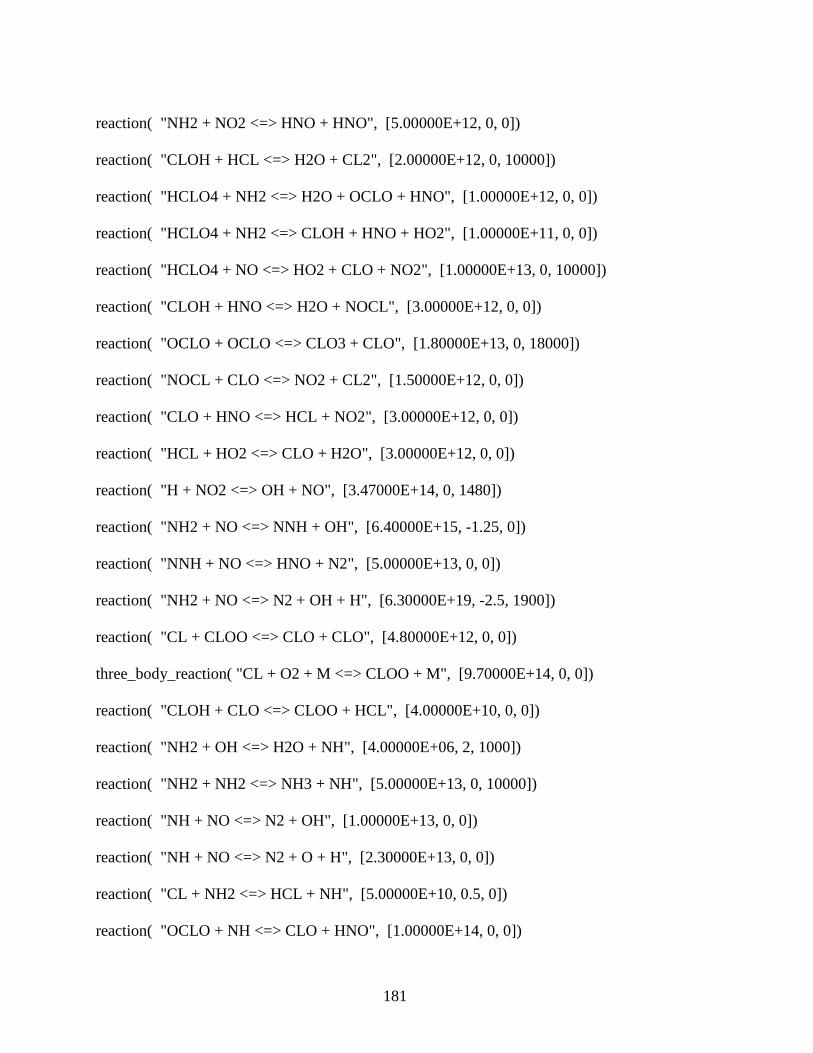
181
reaction( "NH2 + NO2 <=> HNO + HNO", [5.00000E+12, 0, 0]) reaction( "CLOH + HCL <=> H2O + CL2", [2.00000E+12, 0, 10000]) reaction( "HCLO4 + NH2 <=> H2O + OCLO + HNO", [1.00000E+12, 0, 0]) reaction( "HCLO4 + NH2 <=> CLOH + HNO + HO2", [1.00000E+11, 0, 0]) reaction( "HCLO4 + NO <=> HO2 + CLO + NO2", [1.00000E+13, 0, 10000]) reaction( "CLOH + HNO <=> H2O + NOCL", [3.00000E+12, 0, 0]) reaction( "OCLO + OCLO <=> CLO3 + CLO", [1.80000E+13, 0, 18000]) reaction( "NOCL + CLO <=> NO2 + CL2", [1.50000E+12, 0, 0]) reaction( "CLO + HNO <=> HCL + NO2", [3.00000E+12, 0, 0]) reaction( "HCL + HO2 <=> CLO + H2O", [3.00000E+12, 0, 0]) reaction( "H + NO2 <=> OH + NO", [3.47000E+14, 0, 1480]) reaction( "NH2 + NO <=> NNH + OH", [6.40000E+15, -1.25, 0]) reaction( "NNH + NO <=> HNO + N2", [5.00000E+13, 0, 0]) reaction( "NH2 + NO <=> N2 + OH + H", [6.30000E+19, -2.5, 1900]) reaction( "CL + CLOO <=> CLO + CLO", [4.80000E+12, 0, 0]) three_body_reaction( "CL + O2 + M <=> CLOO + M", [9.70000E+14, 0, 0]) reaction( "CLOH + CLO <=> CLOO + HCL", [4.00000E+10, 0, 0]) reaction( "NH2 + OH <=> H2O + NH", [4.00000E+06, 2, 1000]) reaction( "NH2 + NH2 <=> NH3 + NH", [5.00000E+13, 0, 10000]) reaction( "NH + NO <=> N2 + OH", [1.00000E+13, 0, 0]) reaction( "NH + NO <=> N2 + O + H", [2.30000E+13, 0, 0]) reaction( "CL + NH2 <=> HCL + NH", [5.00000E+10, 0.5, 0]) reaction( "OCLO + NH <=> CLO + HNO", [1.00000E+14, 0, 0])

182
reaction( "HCLO4 + NH <=> OH + OCLO + HNO", [1.00000E+14, 0, 0]) reaction( "OH + H2 <=> H2O + H", [1.17000E+09, 1.3, 3626]) reaction( "N + NO2 <=> NO + NO", [1.00000E+14, 0, 0]) reaction( "N + N2O <=> NO + N2", [5.00000E+13, 0, 0]) reaction( "NH + OH <=> N + H2O", [5.00000E+11, 0.5, 2000]) reaction( "NH + OH <=> NO + H2", [1.60000E+12, 0.6, 1500]) reaction( "NH + NH2 <=> NH3 + N", [1.00000E+13, 0, 2000]) reaction( "NH + NH2 <=> N2H2 + H", [5.00000E+13, 0, 0]) reaction( "NH2 + NH2 <=> N2H2 + H2", [5.00000E+11, 0, 0]) reaction( "HO2 + HO2 <=> H2O2 + O2", [2.00000E+12, 0, 0]) three_body_reaction( "H2O2 + M <=> OH + OH + M", [1.30000E+17, 0, 45500]) reaction( "H2O2 + OH <=> H2O + HO2", [1.00000E+13, 0, 1800]) reaction( "N2H2 + NO <=> N2O + NH2", [3.00000E+12, 0, 0]) reaction( "HCL + H <=> H2 + CL", [7.94000E+12, 0, 3400]) reaction( "CLOH + H <=> CLO + H2", [6.00000E+12, 0, 0]) reaction( "CLOH + NH <=> NOCL + H2", [1.00000E+13, 0, 0]) reaction( "HCLO4 + NH <=> CLO3 + N + H2O", [1.00000E+14, 0, 11000]) reaction( "NO + NO <=> N2 + O2", [5.00000E+20, 0, 75506])
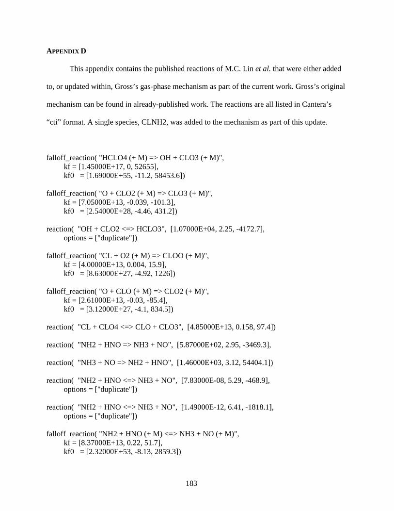
183
APPENDIX D
This appendix contains the published reactions of M.C. Lin et al. that were either added
to, or updated within, Gross’s gas-phase mechanism as part of the current work. Gross’s original
mechanism can be found in already-published work. The reactions are all listed in Cantera’s
“cti” format. A single species, CLNH2, was added to the mechanism as part of this update.
falloff_reaction( "HCLO4 (+ M) => OH + CLO3 (+ M)", kf = [1.45000E+17, 0, 52655], kf0 = [1.69000E+55, -11.2, 58453.6]) falloff_reaction( "O + CLO2 (+ M) => CLO3 (+ M)", kf = [7.05000E+13, -0.039, -101.3], kf0 = [2.54000E+28, -4.46, 431.2]) reaction( "OH + CLO2 <=> HCLO3", [1.07000E+04, 2.25, -4172.7], options = ["duplicate"]) falloff_reaction( "CL + O2 (+ M) => CLOO (+ M)", kf = [4.00000E+13, 0.004, 15.9], kf0 = [8.63000E+27, -4.92, 1226]) falloff_reaction( "O + CLO (+ M) => CLO2 (+ M)", kf = [2.61000E+13, -0.03, -85.4], kf0 = [3.12000E+27, -4.1, 834.5]) reaction( "CL + CLO4 <=> CLO + CLO3", [4.85000E+13, 0.158, 97.4]) reaction( "NH2 + HNO => NH3 + NO", [5.87000E+02, 2.95, -3469.3], reaction( "NH3 + NO => NH2 + HNO", [1.46000E+03, 3.12, 54404.1]) reaction( "NH2 + HNO <=> NH3 + NO", [7.83000E-08, 5.29, -468.9], options = ["duplicate"]) reaction( "NH2 + HNO <=> NH3 + NO", [1.49000E-12, 6.41, -1818.1], options = ["duplicate"]) falloff_reaction( "NH2 + HNO (+ M) <=> NH3 + NO (+ M)", kf = [8.37000E+13, 0.22, 51.7], kf0 = [2.32000E+53, -8.13, 2859.3])

184
reaction( "NH2 + HNO <=> H + H2NNO", [2.43000E+05, 2.15, 759]) reaction( "NH2 + HONO <=> OH + H2NNO", [5.33000E+03, 2.28, 7981.8]) reaction( "NH2 + HONO => NH3 + NO2", [3.17000E+02, 2.83, -3572.6], options = ["duplicate"]) reaction( "NH2 + HONO => NH3 + NO2", [2.96000E-09, 6, 2366.5], options = ["duplicate"]) reaction( "NH3 + NO2 => NH2 + HONO", [2.69000E-01, 4.02, 23247.9], options = ["duplicate"]) reaction( "NH3 + NO2 => NH2 + HONO", [4.24000E-10, 6.48, 27023.2], options = ["duplicate"]) falloff_reaction( "NH2 + HNO3 (+ M) <=> NH3 + NO3 (+ M)", kf = [3.03000E+14, -0.28, -536.5], kf0 = [4.13000E+37, -4.38, 993.5]) reaction( "NH2 + HNO3 => NH3 + NO3", [3.48000E+01, 3.2, -111.3]) reaction( "NH3 + NO3 => NH2 + HNO3", [4.06000E+00, 3.57, 1689]) reaction( "NH2 + HNO3 <=> H2NO + HONO", [8.85000E+01, 2.96, 24440.1], options = ["duplicate"]) reaction( "NH2 + HNO3 <=> H2NO + HONO", [1.73000E+08, 1.17, 29558.6], options = ["duplicate"]) reaction( "H + HCLO4 <=> H2 + CLO4", [6.44000E+06, 1.97, 14876.7]) reaction( "H + HCLO4 <=> OH + HCLO3", [3.66000E+07, 1.96, 15357.5]) reaction( "OH + HCLO4 <=> H2O + CLO4", [2.38000E+01, 3.3, 1847.9]) reaction( "CL + HCLO4 <=> HCL + CLO4", [1.05000E+08, 1.63, 22184.9]) reaction( "CL + HCLO4 <=> CLOH + CLO3", [8.01000E+11, 0.67, 19190.4]) reaction( "CLOH + CLO => CL2O + OH", [1.38000E+07, 1.77, 18650]) reaction( "CLOH + CLO2 <=> HCLO2 + CLO", [6.50000E+02, 2.48, 23180.3]) reaction( "CLOH + CLO3 <=> HCLO3 + CLO", [2.34000E-06, 5.45, 7683.7])

185
reaction( "CLOH + CLO4 <=> HCLO4 + CLO", [8.13000E+05, 1.73, -2020.8]) reaction( "CL2O + OH => CLOH + CLO", [3.89000E+08, 1.39, -824.6]) reaction( "CLOH + CLOH => CL2O + H2O", [6.80000E+01, 3.03, 23220.1], options = ["duplicate"]) reaction( "CLOH + CLOH <=> CL2O + H2O", [2.40000E+01, 3.06, 22397.5], options = ["duplicate"]) reaction( "CLOH + HONO <=> CLNO2 + H2O", [8.13000E+01, 2.86, 2791.7], options = ["duplicate"]) reaction( "CLOH + HONO <=> CLNO2 + H2O", [3.24000E+03, 2.56, 11727.3], options = ["duplicate"]) reaction( "CLOH + HNO <=> CL + NO + H2O", [3.48000E+02, 3.06, 6068.3]) reaction( "CL2O + H2O => CLOH + CLOH", [7.29000E+02, 2.82, 26228.4], options = ["duplicate"]) falloff_reaction( "CLONO2 (+ M) => CLO + NO2 (+ M)", kf = [4.59000E+23, -2.43, 26699.3], kf0 = [3.66000E+47, -6.54, 27446.4]) falloff_reaction( "CLO + NO2 (+ M) => CLONO2 (+ M)", kf = [2.01000E+17, -1.48, 35.8], kf0 = [1.16000E+31, -5.54, 763]) reaction( "CL + NO3 <=> CLO + NO2", [7.17000E+14, -0.6, -115.2]) reaction( "CLO + NO <=> CL + NO2", [8.61000E+14, -0.83, -182.8]) falloff_reaction( "CLNO2 (+ M) <=> CL + NO2 (+ M)", kf = [7.25000E+19, -1.89, 33530.6], kf0 = [1.51000E+62, -6.8, 36578.7]) reaction( "O + HCL <=> OH + CL", [5.58000E+00, 3.67, 2046.6]) reaction( "OH + CLO <=> HCLO2", [3.17000E+15, -1.03, 79.5]) reaction( "HO2 + CLO2 <=> HCLO4", [5.06000E+44, -13.5, 1249.8]) reaction( "HO2 + CLO2 => OH + CLO3", [8.43000E+09, 0.93, 29244.7])

186
falloff_reaction( "CLONO2 (+ M) => CLO + NO2 (+ M)", kf = [4.59000E+23, -2.43, 26699.3], kf0 = [3.66000E+47, -6.54, 27446.4]) falloff_reaction( "CL + NH2 (+ M) <=> CLNH2 (+ M)", kf = [7.22000E+13, 0.196, 32], kf0 = [1.28000E+31, -4.76, 1165])

187
REFERENCES
1 Creighton, J. R., "The Variation of the Ignition Temperature of Solid Explosives as a Function of Heating Rate,"JANNAF Propulsion Systems Hazards Subcommittee Meeting, CPIA No. 599, pgs. 473-482, (1993).
2 Raun, R.L., Butcher, A.G., Caldwell, D.J. and Beckstead, M.W., "An Approach for Predicting
Cookoff Reaction Time and Reaction Severity", 1992 JANNAF Propulsion Systems Hazards Meeting, Vol. I, CPIA No. 582, pgs. 407-504, (1992).
3 Meredith, K. V. and Beckstead M. W., "Fast Cookoff Modeling of HMX", 39th JANNAF
Combustion Meeting. Colorado Springs, CO, pgs. 1-22, (2003). 4 Kuo, K. K., and Lu, Y. C., “Modeling of Pysicochemical Processes of Burning RDX
Monopropellants,” 30th JANNAF Combustion Meeting, CPIA #606, Vol. 2, pgs. 235-257, (1993).
5 Hanson-Parr, D. M., and Parr, T. P., “RDX Laser Assisted Flame Structure,” Proceedings of
the 31st JANNAF Combustion Meeting, Vol. II, CPIA Publication 620, pgs. 407-423, (1994).
6 Melius, C. F., and Binkley, J. S., “Thermochemistry of the Decomposition of Nitramines in the
Gas Phase,” 21st Symposium (Int’l) on Comubstion, The Combustion Institute, pgs. 1953-1963, (1986).
7 Jeppson, M. B., Beckstead, M.W. and Jing, Q., "A Kinetic Model for the Premixed Combustion of a Fine AP/HTPB Composite Propellant", 35th JANNAF Combustion Meeting, (1998).
8 Washburn, E., and Beckstead, M. W., “Modeling Mutilphase Effects in the Combustion of HMX and RDX,” Journal of Propulsion and Power, Vol. 22, No. 5, pgs. 938-946, (2006).
9 Beckstead, M. W., Puduppakkam, K., Thakre, P., and Yang, V., “Modeling of combustion and
ingiitnio of solid-propellant ingredients,” Progress in Energy and combustion Science, Vol 33, pgs. 497-551, (2007).
10 Manelis, G.B. and Strunin, V.A., “The Mechanism of Ammonium Perchlorate Burning,”
Combustion and Flame, Vol. 17, pgs. 69-77, (1971).
188
11 Miller, M.S., “In Search of an Idealized Model of Homogeneous Solid Propellant Combustion,” Combustion and Flame, Vol. 46, pgs. 51-73, (1982).
12 Merzhanov, A.G., “The Theory of Stable Homogeneous Combustion of Condensed
Substances,” Combustion and Flame, Vol. 13, No. 2, pgs. 143-156, (1969). 13 Guirao, C. and Williams, F.A., “A Model for Ammonium Perchlorate Deflagration between 20
and 100 atm,” AIAA Journal, Vol. 9, No. 7, pgs. 1345-1356, (1971). 14 Beckstead, M.W., Derr, R.L., and Price, C.F., “The Combustion of Solid Monopropellants and
Composite Propellants,” Proceedings of the Combustion Institute, Vol. 13, pgs. 1047-1056, (1971).
15 Beckstead, M. W., and Puduppakkam, K. V., and Yang, V., “Modeling and Simulation of
Combustion of Solid Propellant Ingredients Using Detailed Chemical Kinetics,” 49th AIAA Joint Propulsion Conference and Exhibit, AIAA-2004-4036, (2004).
16 Davidson, J. E. and Beckstead, M. W., "A Three-Phase Model of HMX Combustion," 26th
Symposium (Int'l) on Combustion, pgs. 1989-1996, (1996). 17 Gross, M. L., Shurtz, R. C., Hawkins, M. G., Beckstead, M. W., and Hecker, W. C.,
“Development of an Updated Model for Monopropellant AP Combustion: Methodology and Results,” 41st JANNAF Combustion Meeting, pgs. 1-13, (2006).
18 Kee, R. J., Grcar, J. F., Smooke, M.D., and Miller, J. A., “A Fortran Program for Modeling
Steady Laminar One-Dimensional Premixed Flames, “ Sandia Report SAND85-8240, UC-401, Apr (1992).
19 Brown, P. N., Byrne, G. D., and Hindmarsh, A. C., "VODE: A Variable Coefficient ODE
Solver," SIAM J. Sci. Stat. Comput., 10, pgs. 1038-1051, (1989). 20 Vyazovkin, S., and Wight, C. A., “Kinetics of Thermal Decomposition of Cubic Ammonium
Perchlorate,” Chem. Mater., Vol. 11, No. 11, pgs. 3386–3393, (1999). 21 Lang, A. J., and Vyazovkin, S., “Effect of pressure and sample type on decomposition of
ammonium perchlorate,” Combustion and Flame, Vol 145, pgs. 779-790, (2006). 22 Galwey, A. K., and Mohamed, M. A., “The Low Temperature Thermal Decomposition of
Ammonium Perchlorate: Nitryl Perchlorate as the Reaction Intermediate,” Proceedings of the Royal Society of London, Series A, Mathematical and Physical Sciences, Vol. 296, No. 1811, pgs. 425-440, Dec (1984).
23 Boldyrev, V. V., “Thermal decomposition of ammonium perchlorate,” Thermochimica Acta,
Vol 443, pgs. 1-36, (2006).
189
24 Behrens, R., and Minier, L., “The Thermal Decomposition Behavior of Ammonium
Perchlorate and of an Ammonium-Perchlorate-Base Composite Propellant,” 33rd JANNAF Combustion Subcommittee Meeting, Monterey, CA, November (1996).
25 Kraeutle, K. J., “The Thermal Decomposition of Orthorhombic Ammonium Perchlorate Single
Crystals,” Journal of Physical Chemistry, Vol. 74, No. 6, pgs. 1350-1356, March (1970). 26 Kraeutle, K. J., Atwood, A. I., and Curran, P. O., “The Partial Decomposition and Sublimation
of Propellant Grade Ammonium Perchlorate: Effect of Temperature, Time, and Particle Size,” Propulsion Systems Hazards Meeting, CPIA 681, Vol. 1, pgs. 45-56, (1998).
27 Watt Jr., D. M., and Petersen, E. E., “Relationship between the Limiting Pressure and the Solid
Temperature for the Deflagration of Ammonium Perchlorate,” The Journal of Chemical Physics, Vol. 50, No. 5, pgs. 2196-2198, March (1969).
28 Boggs, T. L., “Deflagration Rate, Surface Structure, and Subsurface Profile of Self-
Deflagrating Single Crystals of Ammonium Perchlorate,” AIAA Journal, Vol. 8, No. 5, pgs. 867-873, (1970).
29 Atwood, A. I., Boggs, T. L., Curran, P. O., Parr, T. P., Hanson-Parr, D. M., Price, C. F., and
Wiknich, J., “Burning Rate of Solid Propellant Ingredients, Part 1: Pressure and Initial Temperature Effects,” Journal of Propulsion and Power, Vol. 15, No. 6, pgs. 740-747, Nov-Dec (1999).
30 Beckstead, M. W., and Hightower, J. D., “Surface Temperature of Deflagrating Ammonium
Perchlorate Crystals,” AIAA Journal, Vol. 5, No. 10, pgs. 1785-1790, Oct (1967). 31 Cordes, H. F., “An Estimate of the Melting Point of Ammonium Perchlorate,” AIAA Journal,
Vol. 7, No. 6, pgs. 1193-1195, June (1969). 32 Foltz, M. F., and Maienschein, J. L., “Ammonium perchlorate phase transitions to 256 GPa
and 700 K in a diamond anvil cell,” Materials Letters, Vol 24, Iss 6, pgs. 407-414, (1995).
33 Ermolin, N.E., Korobeinichev, O.P., Tereshchenko, A.G., and Fomin, V.M., “Measurement of
the Concentration Profiles of Reacting Components and Temperature in an Ammonium Perchlorate Flame,” Combustion, Explosion, and Shock Waves, Vol. 18, pgs. 36-38, (1982).
34 Korobeinichev, O. P., “Dynamic Flame Probe Mass Spectrometry and Condensed-System
Decomposition,” Combustion, Explosion, and Shockwave, Vol. 23, No. 5, pgs. 64-76, (1987).
190
35 Ermolin, N. E., Korobeinichev, O. P., Terechchenko, A. G., and Fomin, V. M., “Kinetic Calculations and Mechanism Determination from Chemical Reactions in an Ammonium Perchlorate Flame,” Combustion, Explosion, and Shockwave, Vol. 18, No. 2, pgs. 61-70, (1982).
36 Price, C., Boggs, T., and Derr, R., “Modeling of Solid Monopropellant Deflagration,” AIAA
16th Aerospace Sciences Meeting, Huntsville, AL, Jan 16th-18th, pgs. 1-12, (1978). 37 Price, C. F., Boggs, T. L., and Derr, R. L., “The Steady-State Combustion Behavior of
Ammonium Perchlorate and HMX,” 17th Aerospace Sciences Meeting, New Orleans, LA, Jan 15th-17th, pgs. 1-14, (1979).
38 Ermolin, N.E., Korobeinichev, O.P., Tereshchenko, A.G., and Fomin, V.M., “Kinetic
Calculations and Mechanism Definitions for Reactions in an Ammonium Perchlorate Flame,” Combustion, Explosion, and Shock Waves, Vol. 18, pgs. 180-188, (1982).
39 Nahari, H.K., Mukunda, H.S., and Jain, V.K. “A Model of Combustion Monopropellants (AP)
with Complex Gas Phase Kinetics,” Proceedings of the Combustion Institute, Vol. 20, pgs. 2073-2082, (1984).
40 Ermolin, N.E., “Model for Chemical Reaction Kinetics in Perchloric Acid – Ammonia
Flames,” Combustion, Explosion, and Shock Waves, Vol. 31, No. 5, pgs. 555-565, (1995).
41 Jing, Q., Beckstead, M. W., and Jeppson, M., “Influence of AP Solid Phase Decomposition of
Temperature Profile and Sensitivity,” AIAA 36th Aerospace Sciences Meeting & Exhibit, AIAA-98-0448, (1998).
42 Tanaka, M., and Beckstead, M. W., “A Three-Phase Model of Ammonium Perchlorate,” AIRR
96-2888, (1996). 43 Sheshadri, T. S., and Jain, V. K., “Propellant Gas Phase Chemical Kinetics,” Propellants,
Explosives, and Pyrotechnics, 14, pgs. 193-198, (1989). 44 Beckstead, M. W., Tanaka, M., Jing, Q., and Jeppson, M. B., “An Ammonium Perchlorate
Model Based on a Detail Kinetic Mechanism,” 33rd JANNAF Combustion Meeting, Monterey, CA, pgs. 1-14, (1996).
45 Ermolin, N. E., Korobeinichev, O. P., Tereshchenko, Al, G., and Fomin, V. M., “Kinetic
Calculations and Mechanism Definiton for Reaction in an Ammonium Perchlorate Flame,” Combustion, Explosion, and Shock Wave, Vol. 18, No. 2, pgs. 61-70, (1982).
191
46 Ermolin, N. E., Korobeinichev, O. P., Tereshchenko, A. G., and Fomin, V. M., “Simulation of Kinetics and Chemical Reaction Mechanism of Ammonium Perchlorate Burning,” Sov. J. Chem. Phys., Vol. 1, No. 12, pgs. 2872-2883, (1984).
47 Parr, T., and Hanson-Parr, D., “Thermal Properties Measurements of Solid Rocket Propellant
Oxidizers and Binder Materials as a Function of Temperature,” 34th JANNAF Combustion Meeting, Vol. III, CPIA #662, pgs. 379-404, (1997).
48 Shoemaker, R. L., Stark, J. A., and Taylor, R. E., “Thermophysical Properties of Propellants,”
High Temperatures-High Pressures, ETPC Proceedings, Vol. 17, pgs. 429-435, (1985). 49 Liau, Y. C., Yang, V., Lin M. C., and Park, J., “Analysis of Ammonium Dinitramide (ADN)
Combustion with Detailed Chemistry,” 35th JANNAF Combustion Meeting, CPIA No. 691, pgs. 13-30, (1999).
50 Korobeinichev, O. P., Bolshova, T. A., and Paletsky, A. A., “Modeling the Chemical Reaction
of Ammonium Dinitramide (ADN) in a Flame,” Combustion and Flame, Vol. 126, pgs. 1516-1523, (2001).
51 Ramakrishna, P. A., Paul, P. J., and Mukunda, H. S., “Revisiting the Modeling of Ammonium-
Perchlorate Combustion: Development of an Unsteady Model,” Journal of Propulsion and Power, Vol. 22, No. 3, pgs. 661-668, (2006).
52 Rahman, S., Giovangigli, V., and Borie, V., “Application of Continuation Techniques to
Pressure and Initial Temperature Sensitivity Coefficient Calculation in Ammonium Perchlorate Flames,” 46th AIAA/ASME/SAE/ASEE Joint Propulsion Conference & Exhibit, Nashville, TN, July (2010).
53 Beckstead, M. W., “An Overview of Combustion Mechanisms and Flame Structures of
Advanced Solid Propellants," AIAA 2000-3325, pgs. 267-286, (2000). 54 Ermolin, N. E., Korobeinichev, O. P., Fomin, V. M., and Chernov, A. A., “Study of Flame
Structure for Mixed Solid Fuels Based on Ammonium Perchlorate and Polybutadiene Rubber,” Combustion, Explosion, and Shockwave, Vol. 28, No. 4, pgs. 59-65, (1992).
55 Ermolin, N. E., “Kinetic Perameters of Overall Gas-Phase Reactions for Propellants Based on
Ammonium Perchlorate and Polybutadiene Binder,” Combustion, Explosion, and Shockwave, Vol. 29, No. 4, pgs. 97-104, (1993).
56 Chorpening, B. T., G. M. Knott, and M. Q. Brewster, "Flame Structure and Burning Rate of
Ammonium Perchlorate/Hydroxyl-Terminated Polybutadiene Propellant Sandwiches," Proceedings of The Combustion Institute, 28:1, pgs. 847-853, (2000).

192
57 Knott, G. M. and M. Q. Brewster, "Modeling the Combustion of Propellant Sandwiches," Combustion Science and Technology, 174, pgs. 61-90, (2002).
58 Meyer, R., “Explosives,” 3rd ed. VCH Publishers, New York, pg. 357, (1986). 59 Arisawa, H., and Brill, T. B., “Flash Pyrolysis of Hydroxyl-Terminated Polybutadiene (HTPB)
I: Analysis and Implications of the Gaseous Products,” Combustion and Flame, Vol. 106, pgs. 131-143, (1996).
60 Stephens, H. L., “Physical Constants of Poly(butadiene),” Polymer Handbook, 3rd Ed., John
Wiley & Sons, New York, (1989). 61 Foster, R. L., and Miller, R. R., “The Burn Rate Temperature Sensitivity of Aluminized and
Non-Aluminized HTPB Propellants,” 1980 JANNAF Propulsion Meeting, CPIA #315, Vol. 4, pgs. 667-693, (1981).
62 Tanner, M. W., “Multidimensional modeling of Solid Propellant Burning Rates and Aluminum
Agglomeration and One-Dimensional Modeling of RDX/GAP and AP/HTPB.” PhD Dissertation, Brigham Young University, (2008).
63 Foster, R. L., Condon, J. A., and Miller, R. R., “Low Exponent Technology,” Hercules Report,
AFRPL-TR-81-95, Hercules Inc., Air Force Rocket Propulsion Laboratory, Edwards AFB, CA, (1982).
64 JANNAF Thermochemical Tables, 3rd Edition, Journal of Physical and chemical Reference
Data, Vol. 14, (1985). 65 Atwood, A. I., Ford, K. P., Bui, D. T., Curran, P. O., and Lyle, T., “Radiant Ignition Studies of
Ammonium Perchlorate Based Propellants,” 2nd EUCASS, Brussels, Belgium, July (2007).
66 Hermance, C. E., "Solid-Propellant Ignition Theories and Experiments," Fundamentals of
Solid Propellant Combustion, Vol. 90, pgs. 239-304, (1984). 67 Vilyunov, V. N., and Zarko, V. E., Ignition of Solids, Vol. 60, Elsevier, (1989).
68 Vilyunov, V. N., Vorozhtsov, A. B., Borovskoi, I. G., and Shelupanov, A. A., "Ignition of Condensed Material," Combustion, Explosion & Shockwave, Vol. 24, No. 3, pgs. 39-41, (1988).
69 Dik, I. G., Zurer, A. B., and Knyazeva, A. G., "Ignition of Condensed Material by a Heat Flux
Pulse Across an Opaque Shield Having a High Thermal Conductivity," Combustion, Explosion & Shock Waves, Vol. 25, No. 6, pgs. 3-9, (1989).

193
70 Knyazeva, A. G. and Dik, I. G., "Ignition of a Hot Sheet of Condensed Material Through an Inert Shield," Combustion, Explosion & Shock Waves, Vol. 26, No. 2, pgs. 8-18, (1990).
71 Zarko, V. E., “Stability of Ignition of Condensed Substances,” Combustion, Explosion, and
Shockwave, Vol. 26, No. 6, pgs. 3-16, (1990). 72 Colombier, R., and Pollet, M., “Solid Rocket Motor Ignition Overpressure Prediction”, 27th
Joint Propulsion Conference, Sacramento, CA, (1991). 73 Wooldridge, R. C., and Netzer, D. W., “Ignition and Flammability Characteristics of Solid
Fuel Ramjets”, Journal of Propulsion, Vol. 7, No. 5, pgs. 846-848, (1991). 74 Gehris, R. D. and Price, C. F., "Ignition Modeling Program," 29th JANNAF Combustion
Meeting, Vol. IV, CPIA #595, pgs. 129-137, (1992). 75 Lee, L. S., and Borgardt, F. G., “Ignition Transietn Phenomenology – A Programmatic
Overview”, 29th JANNAF Combustion Meeting, CPIA #595, Vol. 4, pgs. 103-127, (1992). 76 Tsai, C. Y., Reneau, L. R., and Schulze, P. A., “Numerical Simulation of Ignition Transients in
Solid Rocket Motor”, 30th JANNAF Combustion Meeting, Monterey, CA, (1993). 77 Eagar, M. A., Luke, G. D., and Stockham, L. W., “Ignition Transient Modelling for the Space
Shuttle Advanced Solid Rocket Motor”, 29th Joint Propulsion Conference and Exhibit, Monterey, CA, (1993).
78 Dik, I. G., and Selikhovkin, A. M., “Calculation of Ignition Parameters and the Transition to
Compustion in a Heterogeneous System,” Combustion, Explosion, and Shockwave, Vol. 29, No. 3, pgs. 124-129, (1993).
79 Knyazeva, A. H., and Zarko, V. E., “Numerical Simulation of Transients in the Ignition of
Two-component Propellants by Intense Heat Fluxes,” Combustion, Explosion, and Shockwave, Vol. 29, No. 3, pgs. 16-20, (1993).
80 Zarko, V. E., and Knyazeva, A. H., “Simulation of Ignition Transients for Two-component
Solid Propellants under Irradiation, “ AIAA Journal, Paper 94-0790, (1993). 81 Huang, T. H., Thynell, S. T., and Kuo, K. K., "Partially Confined Hot Fragment Conductive
Ignition: Part I-Modeling," 30th JANNAF Combustion Mtg., Vol. I, CPIA No. 606, pgs. 387-400, (1993).
82 Yang, V. and Liau, Y. C., "A Time-Accurate Analysis of RDX Monopropellant Combustion
with Detailed Chemistry," 32nd JANNAF Combustion Mtg., Vol. I, CPIA No. 631, pgs. 57-68, (1995).

194
83 Liau, Y. C. and Yang, V., "Analysis of RDX Monopropellant Combustion with Two-Phase Subsurface Reactions," J. Propulsion & Power, Vol. 11, No. 4, pgs. 729-739, (1995).
84 Liau, Y. C., Kim, E. S., and Yang, V., "A Comprehensive Analysis of Laser-Induced Ignition
of RDX Monopropellant," Combustion and Flame, 126(3), pgs. 1680-1698, (2001). 85 Atwood, A. I., Curran, P. O., Price, C. F., and Wiknich, J., "Burning Rate, Radiant Ignition
and Global Kinetics of Cyclotrimethylene Trinitramine (RDX)," 32nd JANNAF Combustion Mtg. & Propellant Hazards Mtg, Vol. I, CPIA No. 638, pgs. 149-159, (1995).
86 Parr, T., and Hanson-Parr, D., “RDX Ignition Flame Structure,” 27th Symposium (Int’l) on
Combustion, The Combustion Institute, pgs. 2301-2308, (1998). 87 Atwood, A. I., Price, C. F., Boggs, T. L., Curran, P. O., and Zwierzchowski, N. G., “Ignition
and Combustion Properties of Ammonium Perchlorate,” 1990 JANNAF PSHS Meeting, Laurel, Maryland, March (1990).
88 Atwood, A. I., Price, C. F., and Boggs, T. L., “Ignitability Measurements of Solid
Propellants,” Proceedings of the 22nd Annual Conference of ICT, Karlsruhe, Germany, (1991).
89 Waeshe, R. H. W., and Wenograd, J., “Calculation of Solid-Propellant Burning Rates from
condensed-phase Decomposition Kinetics,” Combustion, Explosion, and Shock Waves, Vol. 36, No. 1, pgs. 138-148, (2000).
90 Jojic, I., and Brewster, M. Q., “Condensed-phase Chemical Interaction between Ammonium
Perchlorate and Hydroxy-terminated Polybutadiene,” Journal of Propulsion and Power, Vol. 14, No. 4, pgs. 575-576, (1998).
91 Shannon, L. J., “Composite Solid-Propellant Ignition by Radiant Energy,” AIAA Journal, Vol.
8, No. 2, pgs. 346-353, (1970). 92 Sofue, T., and Iwama, A., “Ignition of Composite Propellant at Sub-atmospheric Pressures by
means of a Carbon Dioxide Laser,” Propellants and Explosives, Vol. 4, pgs. 98-106, (1979).
93 Ahmad S. R., and Russell D. A., “Studies into Laser Ignition of Unconfined Propellants,”
Propellants, Explosives, Pyrotechnics, Vol. 26, pgs. 235-245, (2001). 94 Cain, J., and Brewster, M. Q., “Radiative Ignition of Fine-Ammonium Perchlorate Composite
Propellants,” Propellants, Explosives, Pyrotechnics, Vol. 31, No. 4, pgs. 278-284, (2006).

195
95 Meredith, K. V., and Beckstead, M. W., “Laser-Induced Ignition Modeling of HMX”, 2003 JANNAF Combustion Meeting, Boulder, CO, pgs. 1-22, (2003).
96 Brill, T. B., "Multiphase Chemistry Considerations at the Surface of Burning Nitramine
Monopropellants," J. Propulsion & Power, Vol. 11, No. 4, pgs. 740-751, (1995). 97 Kubota, N., "Survey of Rocket Propellant and Their Combustion Characteristics,"
Fundamentals of Solid-Propellant Combustion, Progress in Astronautics and Aeronautics, Vol. 90, pgs. 1-52, (1984).
98 Hall, P. G., "Thermal Decomposition and Phase Transitions in Solid NItramines,"
Transactions of the Faraday Society, Vol. 2, pgs. 79-102, (1971). 99 Isbell, R. A. and Brewster, M. Q., “Optical Properties of RDX and HMX,” Material Research
Society Symposium Proceedings, 418, edited by Brill, T. B. et al., pgs. 850-90, (1996). 100 Liau, Y. C. and Lyman, J. L., "Modeling Laser-Induced Ignition of Nitramine Propellants
with Condensed and Gas-Phase Absorption," Combust. Sci. and Tech. Vol. 174, No. 3, pgs. 141-171, (2002).
101 Erikson, W. W. and Beckstead, M. W., "Modeling Pressure and Heat Flux Responses of
Nitramine Monopropellants with Detailed Chemistry," Vol. AIAA 99-2498, (1999). 102 Balay, S., Gropp, W. D., McInnes, L. C., and Smith, B. F., "PETSc Home Page,"
http://www.mcs.anl.gov/petsc/petsc-as, (1998). 103 Kee, R. J., Rupley, F. M., and Miller, J. A., SAND87-8215B, Sandia National Laboratories,
(1992). 104 Ali, A. N., Son, S. F., Asay, B. W., Sander, R. K., and Brewster, M. Q., "Laser Ignition of
High Explosives," 36th JANNAF Combust. Subcomm. Mtg. Vol. I, CPIA No. 691, pgs. 51-67, (1999).
105 Creighton, J. R., "The Variation of the Ignition Temperature of Solid Explosives as a
Function of Heating Rate," JANNAF Propulsion Systems Hazards Subcommittee Meeting, CPIA No. 599, pgs. 473-482, (1993).
106 Hobbs, M. L., Baer, M. R., and Gross, R. J., "Modeling ignition chemistry," JANNAF Systems
Hazards Meeting, pgs. 1-10, (1993). 107 Baer, M. R., Gross, R. J., Gartling, D. K., and Hobbs, M. L., "Multidimensional Thermal-
Chemical Cookoff Modeling," 1994 JANNAF Propulsion Systems Hazards Meeting, CPIA No. 615, pgs. 323-332, (1994).

196
108 Erikson, W. W., and Schmitt, R. G., “Coupled Thermal-Chemical-Mechanical Modeling of Validation Cookoff Experiments”, 50th JANNAF Propulsion meeting, Salt Lake City, Utah, (2001).
109 Erikson, W. W., and Schmitt, R. G., “Pre- and Post-ignition Modeling of Validation Cookoff
Experiments”, 38th JANNAF CS, 26th APS, 20th PSHS, and 2nd MSS Joint Meeting, Destin, FL, (2002).
110 Erikson, W. W., and Schmitt, R. G., “Modeling Thermal Decomposition and Deflagration in
Small- and Munition-Scale Navy Coook-off Experiments”, 21st JANNAF PSHS Meeting, CD-ROM ONLY, (2003).
111 Atwood, A. I., Curran, P. O. Erikson, W. W., Heimdahl, O. E. R., McClelland, M. A., and
Rattanapote, M. K., “Full-Scale Cookoff Model Validation Experiments”, 21st JANNAF PSHS Meeting, CD-ROM ONLY, December (2003).
112 Beckstead, M. W. and Hendershot, R. J., "Calculated Conditions for Fast Cookoff," 36th
JANNAF Combustion Meeting, CPIA #691, Vol I, pgs. 123-132, (1999). 113 Ciro, W., Eddings, E. G., and Sarofim, A., "Thermal Behavior of a High-Energy Material
Immersed in a Fire," Proceedings of the Third Joint Meeting of the U.S. Sections of the Combustion Institute, Chicago, IL, (2003).
114 Ford, K. P, Davis, N. C., Farmer, A. D., Washburn, E. B., Atwood, A. I., Wilson, K. J.,
Abshire, J. P., Shewmaker, M. L., Goedert, Z. P., Wheeler, C. J., Curran, P. O., and Covino, J., “Subscale External Fire/Fast Cookoff Testing Results,” 2008 DDESB Seminar Proceedings, (2009).
115 Wilson, E., Gross, M., Washburn, E., et al., “Cookoff Results of Sub-scale Hazard Division
1.3 Propellant Samples,” 34th DoD Explosive Safety Board Seminar, Portland, Oregon, pgs. 1-46, (2010).
116 Washburn, E., Walpole, M., Ford, K., Wilson, E., Atwood, A., Bowman, H., Boggs, T.,
Homer, V., Sawyer, L., and Covino, J., “Ignition of Energetic materials from Heat Fluxes Found in Hazard Situations,” 33nd Explosives Safety Seminar, Palm Springs, CA, August 12-14, (2008).
117 Reaction Design, www.reactiondesign.com, (2003). 118 Goodwin, D. G., www.cantera.org, California Institute of Technology, (2006). 119 Behrens Jr., R., and Bulusu, S., “Thermal Decomposition of Energetic Materials. 3. Temporal
Behaviors of the Rates of Formation of the Gaseous Pyrolysis Products from Condensed-
197
Phase Decomposition of 1,3,5-Trinitrohexahydro-s-triazine,” Journal of Physical Chemistry, Vol. 96, pgs. 8877-8891, (1992).
120 Maxwell, J. C., “A Treatise on Electricity and Magnetism,” Vol. 1, 3rd ed., Oxford University
Press, (1904). 121 Bohren, C. F., and Huffman, D. R., “Absorption and Scattering of Light by Small Particles,”
John Wiley & Sons, Inc., (1983). 122 http://code.google.com/p/scatterlib, (2011)
123 Parr, T., and Hanson-Parr, D., “Thermal Properties Measurements of Solid Rocket Propellant Oxidizers and Binder Materials as a Function of Temperature,” 34th JANNAF Combustion Meeting, Vol. 3, CPIA #662, pgs. 379-404, (1997).
124 Zhu, R. S., and Lin, M. C., “Towards Reliable Prediction of Kinetics and Mechanisms for
Elementary Reactions: Key Combustion Initiation Processes of Ammonium Perchlorate”, Energetic Materials, Part 2, Detonation and Combustion, P. Politzer and J. S. Murray, eds. chp. 11, pgs. 373-443, Elsevier Science Pub., (2003).
125 Lin, M. C., http://chemistry.emory.edu/faculty/lin/pub.htm, Department of Chemistry, Emory
University, (2011). 126 Levy, J. B., and Friedman, R.,“Further Studies of Pure Ammonium Perchlorate Deflagration,”
International Symposium on Combustion, Vol. 8, No. 1, pgs. 663-672, (1961). 127 Hertzberg, M., “The Combustion of Pure and Composite Propellants. The Expansion and
Application of Laminar Flame Theory to Heterogeneous Solid Propellants,” Oxidation and Combustion Reviews, Vol. 5, pgs. 1-81, (1971).
128 Pellett, G. L., “Ammonium Perchlorate Gasification and Combustion at High Heating Rates
and Low Pressures,” International Symposium on Combustion, Vol. 14, Iss 1, pgs. 1317-1330, (1973).
129 Schroeder, T. B., and Brewster, M. Q., “Steady and Unsteady Laser Augmented Combustion
of Ammonium Perchlorate and Atmospheric Conditions,” 30th JANNAF Combustion Meeting, Vol. 1, CPIA No. 6, pgs. 327-336, (1993).
130 Tereshchenko, A. G., and Korobeinichev, O. P., “Correctness of Mass-Spectrometric Probe
Measurements when Investigating the Flame Structure of Condensed Systems,” Combustion, Explosion, and Shock Waves, Vol. 18, No. 6, pgs. 39-45, (1982).
131 Vyazovkin, S., and Wight, C. A., “Kinetics of Thermal Decomposition of Cubic Ammonium
Perchlorate,” Chemistry of Materials, Vol. 11, pgs. 3386-3393, (1999).
198
132 Brill, T. B., Brush, P. J., and Patil, D. G., “Thermal Decomposition of Energetic Materials 60.
Major Reaction Stages of a Simulated Burning Surface of NH4ClO4,” Combustion and Flame, Vol. 94, pgs. 70-76, (1993).
133 Korobeinichev, O. P., “Dynamic Flame Probe Mass Spectrometry and Condensed-System
Decomposition,” Combustion, Explosion, and Shock Waves, Vol. 23, No. 5, pgs. 64-76, (1987).
134 Ermolin, N. E., Korobeinichev, O. P., Tereshchenko, A. G., and Fomin, V. M., “Simulation of
Kinetics and Chemical Reaction Mechanism of Ammonium Perchlorate Burning,” Soviet Journal of Chemical Physics, Vol. 1, Iss. 12, pgs. 2872-2883, (1984).
135 JMP 9.0, <www.jmp.com>, SAS Institute Inc., (2009).
136 Zhu, R., and Lin M. C., “Mechansim and Kinetics for Ammonium Perchlorate Sublimation: A First Principles Study,” Journal of Physical Chemistry C, Vol 112, pgs. 14481-14485, (2008).
137 Longuet, B., and Gillard, P., “Experimental Investigation of the Heterogeneous Kinetic
Process of the Low Thermal Decomposition of Ammonium Perchlorate Particles,” Propellants, Explosives, and Pyrotechnics, Vol. 34, pgs. 59-71, (2009).
138 Ermolin, N. E., “Model for Chemical Reaction Kinetics in Perchloric Acid – Ammonia
Flames,” Combustion, Explosion, and Shock Waves, Vol. 31, No. 5, pgs. 555-565, (1995).
139 Powling, J., “Experiments Relating to the Combustion of Ammonium Perchlorate-Based
Propellants,” International Symposium on Combustion, Vol 11, pgs. 447-456, (1967). 140 Beckstead, M. W., and Hightower, J. D., “Surface Temperature of Deflagrating Ammonium
Perchlorate Crystals,” AIAA Journal, Vol. 5, No. 10, pgs. 1785-1790, (1967). 141 Bakhman, N. N., Kickin, YU. S., Kolyasov, S. M., and Fogelzang, A. E., “Investigation of the
Thermal Sturcture of the Burning Zone in Condensed Mixtures by Fine Thermocouples,” Combustion and Flame, Vol 26, pgs. 235-247, (1976).
142 Korobeinichev, O. P., Zenin, A. A., Tereshchenko, A. G., and Puchkov, V. M., “Investigation
of the Structure of the Combustion Wave of Mixed Systems Based on APC, PMMA, and a Catalyst using Mass-spectrometric and Thermocouple Methods,” Combustion, Explosion, and Shock Waves, Vol. 13, No. 3, pgs. 335-342, (1977).

199
143 McAlevy III, R. F., Cowan, P. L., Summerfield, M., “The Mechanism of Ignition of Composite Solid Propellants by Hot Gases,” Progress in Astronautics and Rocketry, Vol. 1, pgs. 623-652, (1960).
144 Isbell, R. A., and Brewster, M. Q., “Optical Properties of Energetic Materials: RDX, HMX,
AP, NC/NG, and HTPB,” Propellants, Explosives, Pyrotechnics, Vol 23., pgs. 218-224, (1998).
145 Loner, P. S., and Brewster, M. Q., “On the oscillatory laser-augmented combustion of HMX,”
Proceedings of the 34th JANNAF Combustion Subcommittee Meeting, Vol. 2, CPIA, Pub. 662, pgs. 47-60, (1997).
146 Hanson-Parr, D., and Parr, T., “RDX Laser-Assisted Flame Structure,” 31st JANNAF
combustion Meeting, Vol. 2, CPIA 620, pgs. 407-423, (1994). 147 Hanson-Parr, D., and Parr, T., “RDX Flame Structure,” 25th Symposium (International) on
Combustion, pgs. 1635-1643, (1994). 148 Korobeinichev, O. P., Chernox, A. A., Emel’yanov, I. D., Ermolin, N. E., and Trofimycheva,
T. V., “Investigation of the Kinetics and the Chemical reaction Mechanism in the Flame of a Mixed Compound, Based on Ammonium Perchlorate and Polybutadiene Rubber,” Combustion, Explosion, and Shock Waves, Vol. 26, No. 3, pgs. 292-300, (1989).
149 Godai, T. and Shimizu, M., “Pressure exponent of controllable solid rocket propellants,”
Proceedings of AIAA/SAE 8th Joint Propulsion Specialist Conference, AIAA Paper 72-1135, New Orleans, Louisiana, (1972).
150 Sutton, G. P., “Rocket Propulsion Elements, Sixth Edition,” John Wiley & Sons., 1992.
151 Kohga, M., “Burning Characteristics and Thermochemical Behavior of AP/HTPB Composite Propellant Using Coarse and Fine AP Particles,” Propellants, Explosives, and Pyrotechnics, Vol.36, pgs. 57-64, (2011).
152 Foster, R. L., Condon, J. A., and Miller R. R., “Low Exponent Technology,” Hercules Report,
AFRPL-TR-81-95, Hercules Inc., Air Force Rocket Propulsion Laboratory, Edwards AFB, CA, (1982).
153 Son, S. F., and Brewster, M. Q., “Radiation-Augmented Combustion of Homogeneous
Solids,” Combustion Science and Technology, Vol. 107, pgs. 127-154, (1995). 154 Fitzgerald, R. P., and Brewster, M. Q., “Flame and Surface Structure of Laminate Propellants
with Coarse and Fine Ammonium Perchlorate,” Combustion and Flame, Vol. 136, No. 3, pgs. 313-326, (2004).

200
155 Rasmussen, B., and Frederick, R. A. Jr., “Nonlinear Hereogeneous Model of Composite Solid-Propellant Combustion,” Journal of Propulsion and Power, Vol. 18, No. 5, pgs. 1086-1092, (2002).
156 Bellec, R., Duterque, J., and Lengelle, G., “Modeling of Aluminized Solid Propellants,”
ONERA, Technical Report RT 37/7128 EN, Palaiseau, France, (1996). 157 Cohen-Nir, E., “Temperature Sensitivity of the Burning Rate of Composite Solid
Propellants,” Combustion Science and Technology, Vol. 9, pgs. 183-194, (1974). 158 Foster, R.L. and R.R. Miller, “The Burn Rate Temperature Sensitivity of Aluminized and
Non-Aluminized HTPB Propellants,” 1980 JANNAF Propulsion Meeting, CPIA #315, Vol. IV, pgs. 667-693, (1981).
159 Kubota, N., and Miyazaki, S., “Temperature Sensitivity of Burning Rate of Ammonium
Perchlorate Propellants,” Propellants, Explosives, Pyrotechnics, Vol. 12, pgs. 183-187, (1987).
160 Korobeinichev, N. E., Ermolin, N. E., Chernov, A. A., and Emel’yanov I. D., “Flame
Structure, Kinetics and Mechanism of Chemical Reactions in Flames of Mixed Composition Based on Ammonium Perchlorate and Polybutadiene Rubber,” Combustion, Explosion, and Shock Waves, Vol. 28, No. 4, pgs. 366-371, (1992).
161 Atwood, A. I., personal communication, (2008).
162 Osman, M. B. S., Dakroury, A. Z., Dessouky, M. T., Kenawy, M. A., and El-Sharkawy, A. A., “Measurement of Thermophysical Properties of Ammonium Salts in the Solid and Molten States,” Journal of Thermal Analysis, Vol. 46, pgs. 1697-1703, (1996).
163 Atwood, A. I., Boggs, T. L., Curran, P. O., Parr, T. P., Hanson-Parr, D. M., Price, C. F., and
Wiknich, J., “Burning Rate of Solid Propellant Ingredients, Part 1: Pressure and Initial Temperature Effects,” Journal of Propulsion and Power, Vol. 15, No. 6, pgs. 740-747, Nov-Dec (1999).
164 Ross, S. D., “Forbidden Transitions in the Infrared Spectra of Some Tetrahedral Anions – I.
Perchlorates,” Spectrochimica Acta, Vol. 18, pgs. 225-228, (1962). 165 Maycock, J. N., Pai Vernecker, V. R., and Gorzynski Jr., C. S., “Electrical Conductivity of
Ammonium Perchlorate,” Solid State Communications, Vol. 5, pgs. 225-227, (1967). 166 Owen, G. P., Thomas, J. M., and Williams, J. O., “Electrical Conduction in Ammonium
Perchlorate,” Journal of the Chemical Society, Faraday Transactions 1, Vol. 68, pgs. 2356-2366, (1972).

201
167 Jacobs, P. W. M., Lovatt, F. E., and Ng, W. L., “Electrical Conductivity of Pure and Doped Ammonium Perchlorate Crystals,” Canadian Journal of Chemistry, Vol. 50, No. 19, pgs. 3154-3160, (1972).
168 Ivashchenko, Yu. S., Sadyrin, A. L., and Pavlenko, V. L., “Electrical Conductivity of the
Burning Surface of Ammonium Perchlorate, “ Combustion, Explosion, and Shock Waves, Vol, 2. No. 4, pgs. 414-416, (1986).
169 Yang, V., Brill, T. B., and Ren, W. Z., “Flash Pyrolysis of Ammonium Perchlorate-Hydroxyl-
Terminated-Polybutadiene Mixtures Including Selected Additives,” Solid Propellant Chemistry, Combustion, and Motor Interior Ballistics, Chapter 1.1, Progress in Astronautics and Aeronautics, Vol. 185, pgs. 3-32, (2000).
170 Beckstead, M. W., personal communication, (2011).
171 Eagar, M. A., Luke, G. D., and Stockham, L. W., “Ignition Transient Modeling for the Space Shuttle Advanced Solid Rocket Motor,” 29th Joint Propulsion Conference, AIAA 93-2062, Monterey, CA, pgs. 1-11, (1993).
172 Jojic, I., and Brewster, M. Q., “Condensed-Phase Chemical Interaction Between Ammonium
Perchlorate and Hydroxy-Terminated Polybutadiene,” Journal of Propulsion and Power, Vol. 14, No. 4, pgs. 575-576, (1998).
173 Ahmad, S. R., and Russell, D. A., “Studies into Laser Ignition of Unconfined Propellants,”
Propellants, Explosives, Pyrotechnics, Vol. 26, pgs. 235-245, (2001). 174 Kimura, E., and Oyumi, Y., “Shock ignitability test for azide polymer propellants,” Journal of
Energetic Materials, Vol. 16, pgs. 173–186, (1998). 175 Zanotti, C., and Galfetti L., “Experimental and Numerical Study of Ignition Transients of
Solid Propellants,” Flame structure (Ed. O.P. Korobeinichev), Novosibirst, Nauka, Vol. 2, pgs. 393-396, (1991).
176 Atwood, A. I., Price, C. F., and Boggs, T. L., “A Comparison of Radiant Ignition and Ballistic
Impact Chamber Results, “ 1992 JANNAF PSHS Mtg., pgs. 1-17, (1992). 177 Cocchiaro, J. E., “Subscale Fast Cookoff Testing and Modeling for the Hazard Assessment of
Large Rocket Motors,” Chemical Propulsion Information Agency, CPTR-72, (2001). 178 Lengelle, G., Bizot, A., Duterque, J., and Amiot, J., “Ignition of Solid Propellants,” Rech.
Aerosp., Vol. 2, pp. 1-20, (1991). 179 Najm, H. N., Wyckoff, P. S., and Knio, O. M., “A Semi-implicit Numerical Scheme for
Reacting Flow,” Journal of Computational Physics, Vol. 143, pgs. 381-402, (1998).

202
180 Najm, H. N., and Knio, O. M., “Modeling Low Mach Number Reacting Flow with Detailed
Chemistry and Transport,” Journal of Scientific Computing, Vol. 25, Nos. 1&2, pgs. 263-287, (2005).
181 Singer, M. A., and Pope, S. B., “Exploiting ISAT to solve the reaction-diffusion equation,”
Combustion Theory and Modeling, Vol. 8, pgs. 361-383, (2004). 182 Pope, S.B., and Ren, Z. “Efficient Implementation of Chemistry in Computational
Combustion,” Flow Turbulence Combustion, Vol. 82, pgs. 437-453, (2009).


![Solid Propellant Autonomous DE-Orbit System [SPADES]](https://img.dokumen.tips/doc/110x75/620280c02fda4a4c6d4aa41e/solid-propellant-autonomous-de-orbit-system-spades.jpg)


