Embed Size (px)
Citation preview

MODELING, SIMULATION, AND CONTROL OF
BIOTRICKLING FILTER FOR REMOVAL OF AIR POLLUTANTS
by
Wasim Ahmed
A Thesis Presented to the Faculty of the American University of Sharjah
College of Engineering in Partial Fulfillment of the Requirements
for the Degree of
Master of Science in Chemical Engineering
Sharjah, United Arab Emirates
June 2012

2
© 2012 Wasim Ahmed. All rights reserved.

3
Approval Signatures We, the undersigned, approve the Master’s Thesis of Wasim Ahmed. Thesis Title: Modeling, Simulation, and Control of Biotrickling Filter for Removal of Air
Pollutants Signature Date of Signature
___________________________ _______________ Dr. Zarook Shareefdeen Associate Professor, Department of Chemical Engineering Thesis Advisor ___________________________ _______________ Dr. Nabil Abdel Jabbar Professor, Department of Chemical Engineering Thesis Co-Advisor ___________________________ _______________ Dr. Rachid Chebbi Professor, Department of Chemical Engineering Thesis Committee Member ___________________________ _______________ Dr. Ahmed Aidan Lab Instructor, Department of Chemical Engineering Thesis Committee Member ___________________________ _______________ Dr. Abdul-Rahman Al-Ali Professor, Department of Computer Science and Engineering External Thesis Committee Member ___________________________ _______________ Dr. Dana Abouelnasr Head, Department of Chemical Engineering ___________________________ _______________ Dr. Hany El-Kadi Associate Dean, College of Engineering ___________________________ _______________ Dr. Yousef Al-Assaf Dean of College of Engineering ___________________________ _______________ Dr. Khaled Assaleh Director of Graduate Studies

4
Abstract
Stringent environmental regulations for control of pollutants have led to the use of
effective air pollution control strategies. Biotrickling filter, one of the biological reactors,
offers a great advantage of being a cost effective and environmental friendly technology. This
emerging technology has not yet received widespread application. Moreover, there is still a
need to develop an appropriate biotrickling filter model for general acceptance and equally
important to design an optimum control strategy before utilizing this technology on a large
scale. Hence, this thesis aims to develop a representative dynamic model for the biotrickling
filter based on the review of existing models, provide accurate analytical and numerical
solution of the model under different conditions, and also select an optimum control strategy
amongst the different control systems designed in this study. A theoretical model was
selected, validated and modified to account for continuous, larger biotrickling filter. The
modified model was solved using the pseudo-steady state assumption to reduce
computational effort and time. Based on sensitivity analysis of the modified model, it was
found that gas velocity and inlet concentration had strong effect on the outlet concentration of
biotrickling filter. To implement the control strategies, simple data driven models were
obtained using the data from simulation of the modified model. These data driven models
were needed since the modified model simulation would require considerable computational
effort and time. In particular, transfer function and neural network models were successfully
obtained with R2 values above 0.97. Five control strategies were designed, implemented and
analyzed through set-point and disturbance changes. Three of the five controllers were based
on transfer function biotrickling filter model while the rest used steady state neural networks
as the biotrickling filter plant model. Overall, it was found that the proportional-integral,
proportional-integral with feedforward and the transfer function based model predictive
controllers provided satisfactory system performance. In case of the neural network based
model predictive controller, excellent set-point tracking had been observed but an offset error
had been observed in case of disturbance change. While the addition of an integral controller
to the neural network based model predictive controller eliminated the offset errors, large
overshoots had been observed in response to both set-point and disturbance changes.
Search Terms: biotrickling filter, mathematical modeling, step response model, neural network
model, biotrickling filter control strategies, conventional control strategies, advanced control

5
Table of Contents
ABSTRACT ..........................................................................................................................4
LIST OF FIGURES .....................................................................................................................7
LIST OF TABLES ......................................................................................................................9
NOMENCLATURE ................................................................................................................. 10
CHAPTER 1. INTRODUCTION ................................................................................................ 14
1.1 BACKGROUND ......................................................................................................................................... 14 1.2 OVERVIEW OF BIOTRICKLING FILTER MODELING AND CONTROL......................................................................... 17 1.3 PROBLEM STATEMENT .............................................................................................................................. 18 1.4 THESIS ORGANIZATION .............................................................................................................................. 18
CHAPTER 2. MODELING AND SIMULATION OF BIOTRICKLING FILTER .................................... 20
2.1 REVIEW OF EXISTING BTF MODELS ............................................................................................................. 20 2.1.1 Model by Kim & Deshusses ......................................................................................................... 20 2.1.2 Model by Alonso et al. ................................................................................................................ 21 2.1.3 Model by Liao et al. ..................................................................................................................... 23 2.1.4 Model by Sharvelle et al. ............................................................................................................. 24 2.1.5 Model by Lee & Heber ................................................................................................................. 25 2.1.6 Summary of models reviewed ...................................................................................................... 26
2.2 BTF MODEL SELECTION ............................................................................................................................ 28 2.3 BTF MODEL FORMULATION ....................................................................................................................... 28
2.3.1 Model assumptions ...................................................................................................................... 28 2.3.2 Model equations .......................................................................................................................... 29 2.3.3 Modified BTF Model ..................................................................................................................... 32
2.4 MODEL SIMULATION ................................................................................................................................ 35 2.4.1 BTF process conditions and model parameters ........................................................................... 35 2.4.2 Solution Methodology ................................................................................................................. 38 2.4.3 Results and discussion ................................................................................................................. 39
2.4.3.1 Simulation and validity of original model ............................................................................................. 39 2.4.3.2 Simulation of the modified model ........................................................................................................ 40 2.4.3.3 Sensitivity analysis of the modified model ........................................................................................... 42

6
CHAPTER 3. BIOTRICKLING FILTER SYSTEM IDENTIFICATION AND CONTROL .......................... 47
3.1 BTF SYSTEM IDENTIFICATION ..................................................................................................................... 47 3.1.1 BTF input-output structure .......................................................................................................... 49 3.1.2 Open loop step response models ................................................................................................. 50 3.1.3 Neural network model ................................................................................................................. 51 3.1.4 Results and discussion ................................................................................................................. 54
3.1.4.1 Identified transfer function BTF models ............................................................................................... 54 3.1.4.2 BTF neural network model identification and simulation .................................................................... 58
3.2 BTF PROCESS CONTROL ............................................................................................................................ 62 3.2.1 General BTF control structure ...................................................................................................... 64 3.2.2 Conventional control strategies ................................................................................................... 65
3.2.2.1 Feedback PI control .............................................................................................................................. 65 3.2.2.2 Feedback-feedforward hybrid control .................................................................................................. 68
3.2.3 Advanced control strategies ........................................................................................................ 71 3.2.3.1 Model predictive control ...................................................................................................................... 71 3.2.3.2 NNMPC with FB integral control ........................................................................................................... 75
3.2.4 Results and discussion ................................................................................................................. 76 3.2.4.1 Analysis of feedback PI controller ......................................................................................................... 76 3.2.4.2 Analysis of FB-FF control system .......................................................................................................... 79 3.2.4.3 Analysis of transfer function MPC controller. ....................................................................................... 80 3.2.4.4 Analysis of neural network MPC controller .......................................................................................... 83 3.2.4.5 Analysis of combined NNMPC and integral control .............................................................................. 86 3.2.4.6 Comparison of BTF control strategies ................................................................................................... 89
CHAPTER 4. CONCLUSION .................................................................................................... 92
REFERENCES ........................................................................................................................ 95
APPENDIX ........................................................................................................................ 98

7
List of Figures Figure 1-1: Schematic of a biotrickling filter [3] ........................................................................... 15 Figure 2-1: Schematic of the BTF model concept proposed by Kim and Deshusses [5] .............. 21 Figure 2-2: Proposed models by Alonso et al. [10]: a) spheres based, b) parallel
pipes based, and c) parallel plates based .................................................................... 22 Figure 2-3: General model concept by Alonso et al. [10] .............................................................. 22 Figure 2-4: Schematic of the capillary tube model proposed by Liao et al. [11] ........................... 23 Figure 2-5: Schematic of the model structure proposed by Liao et. al [11]
under a) co-current and b) counter-current flows ...................................................... 24 Figure 2-6: Concentration gradient of hydrophobic compound without
liquid barrier in the model proposed by Lee and Heber ............................................. 25 Figure 2-7: Model structure proposed by Kim and Deshusses [5]. ................................................ 30 Figure 2-8: BTFs in series model structure .................................................................................... 34 Figure 2-9: Solution scheme for BTFs in series model ................................................................. 39 Figure 2-10: Comparisons between original model predictions and experimental data. ............... 40 Figure 2-11: Simulation of the proposed BTFs in series model at steady state ............................. 41 Figure 2-12: Dynamic simulation of the proposed BTFs in series model ..................................... 42 Figure 2-13: Effect of inlet concentration on BTF performance ................................................... 43 Figure 2-14: Effect of gas velocity on BTF performance .............................................................. 44 Figure 2-15: Effect of liquid-gas velocity ratio on BTF performance ........................................... 45 Figure 3-1: Input/output structure for system identification of the BTF process .......................... 49 Figure 3-2: General FNN structure [22] ........................................................................................ 53 Figure 3-3: (a) Output comparison between modified model data and fitted TF model for
(b) step changes in gas velocity (input 1) at base inlet concentration (ΔCg0 = 0) ....... 55 Figure 3-4: (a) Output comparison between modified model data and fitted TF model for
(b) step changes in inlet concentration (input 2) at base gas velocity (Δug = 0) ......... 56

8
Figure 3-5: (a) Output comparison between modified model data and NN model for (b) step change in gas velocity at base inlet concentration........................................ 59
Figure 3-6: (a) Output comparison between modified model data and NN model for
(b) step change in inlet concentration at base gas velocity......................................... 60 Figure 3-7: Feedback structure for BTF process control ............................................................... 65 Figure 3-8: Block flow diagram of a FB control system [18]. ....................................................... 66 Figure 3-9: Block flow diagram of a FB-FF control system .......................................................... 69 Figure 3-10: FB-FF control structure for BTF process .................................................................. 70 Figure 3-11: Basic concept of MPC [18] ....................................................................................... 72 Figure 3-12: Basic MPC structure [26] .......................................................................................... 72 Figure 3-13: Block flow diagram of NNMPC - FB integral control system.................................. 76 Figure 3-14: (a) Output and (b) input responses for set-point change in case of PI control .......... 77 Figure 3-15: (a) Output and (b) input responses for disturbance change in case of PI control ...... 78 Figure 3-16: (a) Output and (b) input responses for disturbance change in
case of FB-FF control ............................................................................................... 80 Figure 3-17: (a) Output and (b) input responses for set-point change in
case of transfer function MPC .................................................................................. 81 Figure 3-18: (a) Output and (b) input responses for disturbance change in
case of transfer function MPC .................................................................................. 82 Figure 3-19: (a) Output and (b) input responses for set-point change in case of NNMPC ............ 84 Figure 3-20: (a) Output and (b) input responses for disturbance change in case of NNMPC ....... 85 Figure 3-21: (a) Output and (b) input responses for set-point change in
case of NNMPC-integral control .............................................................................. 87 Figure 3-22: (a) Output and (b) input responses for disturbance change in
case of NNMPC-integral control .............................................................................. 88 Figure 3-23: Output responses of TF based controllers in case of step changes ........................... 90 Figure 3-24: Output responses of TF based controllers in case of disturbance change ................. 91

9
List of Tables
Table 2-1: Summary of Reviewed Models .................................................................................... 27 Table 2-2: BTF process properties and conditions ........................................................................ 36 Table 2-3: BTF model parameters ................................................................................................. 37 Table 2-4: Base conditions for BTF process .................................................................................. 37 Table 3-1: Results summary of fitted BTF transfer function models ............................................ 57 Table 3-2: Summary of fitted BTF neural network model ............................................................ 58 Table 3-3: Control valve and sensor/transmitter properties for PI control system ........................ 68 Table 3-4: Transfer function MPC controller settings ................................................................... 80 Table 3-5: Trained NN and NNMPC controller setting results ..................................................... 83 Table 3-6: NNMPC and integral controller properties .................................................................. 86

10
Nomenclature Anw - non-wetted area (m2)
Aw - wetted area (m2)
a - specific interfacial area (m-1)
aw - specific wetted area (m2/(m3 of packed bed))
C - H2S concentration (g m-3)
Cgi1 - gas phase concentration of H2S at gas-liquid interface (g m-3)
Cgi2 - gas phase concentration of H2S at gas-biofilm interface (g m-3)
CLi2 - liquid phase concentration of H2S at liquid-biofilm interface (g m-3)
Cwb - concentration of H2S in the wetted biofilm (g m-3)
Cnwb - concentration of H2S in the non-wetted biofilm (g m-3)
Dg - H2S diffusion coefficient in air (m2 h-1)
DL - diffusivity of H2S in trickling liquid (m2 h-1)
d - disturbance variable
EBRT - empty bed residence time, Bed heightug
(h or sec)
F - volumetric flow rate (m3h-1)
Fr - Froude number
FT - biofilm thickness (m)
∆FT - discretized biofilm thickness (m)
G - superficial mass velocity of gas (kgm-2h-1)
G(s) - transfer function
Gc - controller transfer function
Gd - disturbance transfer function
Gf - feedforward controller transfer function

11
Gm / Gt - sensor transfer function
Gp - process transfer function
Gv - control valve transfer function
gc - gravitational constant (mh-2)
H - Henry’s constant ( - )
i, j - index for finite elements in the dynamic model
K - gain
Kc - proportional gain
KIP - current to pressure transducer gain
Km - measurement gain
Ks - Michaelis-Menten constant (g m-3)
Kv - control valve gain
kg1 - mass transfer coefficient from gas to liquid (mh-1)
kg2 - mass transfer coefficient from gas to non-wetted biofilm (mh-1)
kL - mass transfer coefficient in liquid (mh-1)
L - superficial mass velocity of liquid (kgm-2h-1)
N - number of layer subdivisions
Re - Reynolds number
Rm - maximum reaction rate (gm-3h-1)
u - manipulated variable
U - input
UL/g - liquid-gas velocity ratio
V - volume (m3)
Vg/L - gas-liquid volume ratio
We - Weber number

12
WR - wetting ratio
X - test variable or data point
∆X - deviation variable
Y - output
Greek letters
∆ - deviation
𝜃 - time delay (s)
𝜇 - viscosity (kgm-1h-1)
𝜌 - density (kgm-3)
𝜎𝑝 - surface tension of packing (kg h-2)
𝜎 - surface tension of water (kg h-2)
𝜏 - time constant (s)
𝜏𝐷 - derivative time
𝜏𝐼 - integral time
Subscripts
g - gas phase
L - liquid phase
max - maximum
min - minimum
nm - nominal
sp - set-point

13
Superscript
n - normalized
Abbreviations
ANN - artificial neural network
BTF - biotrickling filter
ERN - external neural network
FB - feedback
FF - feedforward
FNN - feedforward neural network
LGVR - liquid-gas velocity ratio
MPC - model predictive control
NN - neural network
ODE - ordinary differential equation
PDE - partial differential equation
PUF - polyurethane foam
TF - transfer function
VOC - volatile organic compound

14
Chapter 1. Introduction
Stringent environmental regulations for control of pollutants have led to the use of
effective air pollution control strategies. Biotrickling filter (BTF), one of the biological
reactors, offers a great advantage of being a cost effective and environmental friendly
technology [1]. This emerging technology has not yet received widespread application.
However, in the future, environmental regulations will become more restricted, forcing
industries to implement such environmental friendly technologies. As mentioned by
Devinny and Ramesh [2], no single BTF model exists for general acceptance and most of
the models are specific to experiments under study. On the other hand, implementing any
industrial process without control is impossible by all respect and controlling treatment
processes is by itself a necessity to avoid release of pollutants above the legal limits.
Hence, accurate model prediction and effective control of a BTF is necessary to render
this prospective technology feasible for industrial application.
1.1 Background
Harmful pollutants such as volatile organic compounds and odorous compounds
released from several industries pose a serious threat to human health and environment
[1]. An even worse situation is the increasing release of these compounds as more
industries develop to cope with the increasing population. As a result, there is an
increasing demand to control such emissions for the well-being of humans and the
environment. Stringent environmental regulations for the emissions of such pollutants
have led industries to opt for effective air pollution control technologies to comply with
the governmental regulations as well as minimize costs for treatment [1]. Physical and
chemical treatment technologies are the conventional methods used in industries to treat
these pollutants. However, biological treatment technologies have increasingly become
popular due to some major advantages they offer in comparison to the conventional
methods. Biological reactors offer greater advantage of being cost-effective as well as
environmental friendly [1]. There are three main types of bioreactors: 1) biofilters, 2)
biotrickling filters, and 3) bioscrubbers. The basic removal mechanisms are somewhat

15
similar in all three bioreactors. A biotrickling filter (BTF), the bioreactor of interest,
consists of a packed-bed column through which there is continuous flow of liquid and
pollutant laden gas stream [3]. The continuous liquid stream (trickling liquid) consists of
an aqueous solution of nutrients to sustain micro-organisms immobilized on the inert
packing material. The reactor is operated either co-currently or counter-currently with
respect to the gas and liquid phases. A schematic diagram of the biotrickling trickling
filter is shown in Fig. 1-1.
Figure 1-1. Schematic of a biotrickling filter [3]
The mechanism of a BTF consists of absorption of pollutant from the gas phase
into the liquid phase and then into an aqueous biological layer known as biofilm. Once in
the biofilm, the pollutant diffuses and gets biodegraded along the depth of the biofilm.
Since the packing is inert, biotrickling filters need to be inoculated [3]. Some of the
factors affecting the performance of a biotrickling filter are as follows:

16
− Nutrient supply
In general, continuous nutrient supply is needed to support the microbial
community as well as control biological operating parameters such as pH, amount of
nutrients, etc [1]. Moreover, the liquid supply may also reduce clogging problems by
sloughing of biofilm [2]. However, excessive nutrient supply results in excessive biomass
formation and clogging of filter bed, typically in case of VOC control [4]. On the other
hand, in case of odor and H2S control, clogging does not occur since thin biofilms are
formed due to the inefficiency of the micro-organisms with respect to growth and
biomass formation.
− Mode of operation
For VOC control, co-current operation is preferred. In case of counter current
operation, stripping of the contaminant from the recycled liquid occurs at the gas outlet,
resulting in lower removal efficiency. For H2S and odor control, where such processes
are mass transfer limited due to the low solubility of the contaminants in the liquid,
counter current operation is preferred. [4]
− Trickling rate
The effect of trickling rate depends on the nature of process that limits the
pollutant removal. For treatment of acid producing pollutants such as H2S, pH control can
be achieved with the trickling liquid. For a low trickling rate, the rate of removal of acid
products will be low, causing inhibition of the process culture. However, high trickling
rate results in the formation of a thick liquid layer over the biofilm. A thick layer will
result in high mass transfer resistance, thereby reducing the removal efficiency.
− Oxygen content
Oxygen, needed by the micro-organisms, has a high value of Henry’s law
constant, implying that penetration depth of oxygen in biofilm will be lower than the
pollutant. Hence, limitation of oxygen occurs that might result in the development of
anaerobic zones. [4]

17
− Inoculation
As mentioned above, the inert packing requires inoculation since there are no
microbial populations on the inert packing initially. Inoculation is usually done using
activated sludge, compost extract, specialized enriched cultures, etc [4]. Initially, water
supply and purge through the BTF is reduced to avoid possible wash out and facilitate
attachment of micro-organisms onto the packing.
1.2 Overview of Biotrickling Filter Modeling and Control
To achieve an understanding and improvement of reactor performance, several
mathematical models have been developed for BTFs [2]. As mentioned earlier, a BTF
process consists of contaminants being transferred from gas phase to the trickling liquid
and then into the biofilm, where diffusion and biodegradation of contaminants take place.
Hence, the major concepts involved in the existing biotrickling filter models are: 1) mass
transfer, 2) biodegradation, and 3) biomass growth. In the gas phase, most models assume
plug flow conditions, neglecting axial dispersion effects [2]. However, there are few
models that have considered axial dispersion effects in cases where axial gradients are
significant. With regard to pollutant mass transfer through the liquid layer, the liquid
phase is usually neglected due to the assumption that a thin liquid layer offers less
resistance to mass flow [5]. However, there are some models that use Henry’s law
equilibrium at gas-liquid interface. In case of the biofilm phase, mass transfer has been
described by Fick’s law [2]. The most important process that limits the performance of
any bioreactor considered is biodegradation [2]. Most of the models incorporate Monod
type kinetics for biodegradation that considers contaminant as the only limiting substrate.
More realistic models have considered oxygen limitations and also inhibition effects
sometimes in addition to the substrate limitation by using the Michaelis-Menten
relationships and Haldane type kinetics. However, the major challenge in using such
kinetics is the accurate prediction of biokinetic parameters [2]. Finally, many models
have incorporated the effect of biomass growth since it affects the formation of biofilm
and hence, performance of the BTF. As biomass increases, biofilm gets thicker. In this
case, deeper portions of the biofilm will be deprived of oxygen and nutrients, resulting in
18
the formation of inactive zones [2]. Moreover, thickening of biofilm causes reduction of
pore size and increase in the pressure drop, thereby resulting in the clogging of the filter
bed. While some models have considered changes in biofilm thickness due to biomass
growth, other models usually assume constant biofilm thickness since there is constant
sloughing of biofilm by the trickling liquid. Despite the achievements made in BTF
modeling, there hasn’t been a generally accepted BTF model because most of the models
are specific to a particular application under study [2].
Apart from theoretical modeling, there are few studies that focused on using
simpler data driven or black-box models to predict the performance of a BTF [6], [7], [8].
While there have been major improvements in the model prediction of BTF performance,
there is a need to design an optimum control scheme for a BTF as well; a major field that
has not been quite addressed yet. Only one such research could be found where an
effective control system for a BTF treating hydrogen sulphide (H2S) was designed [9].
1.3 Problem Statement
Based on the overview presented in the previous section, it can be deduced that
there is a need to develop an appropriate BTF model for general acceptance and equally
important to design an optimum control strategy before utilizing this technology on a
large scale. Hence, this thesis aims to develop a representative dynamic model for the
biotrickling filter based on the review of existing models, provide accurate analytical and
numerical solution of the model under different conditions, and also select an optimum
control strategy amongst the different control systems designed in this study.
1.4 Thesis Organization Chapters 2 of this thesis pertains to screening of different biotrickling filter
models available in the literature, and then modify the most appropriate model to be
simulated and validated against literature experimental data. Next, simulation and
sensitivity analysis was performed on the proposed model quantifying the effect of
different operating conditions on process performance. Chapter 3 of the thesis will be

19
dedicated to control system design and system identification of the BTF process. Black-
box reduced-order models for the BTF were fitted with the data generated from the
rigorous model. The control system design was implemented on these identified models
via classical and advanced control algorithms outlined in Chapter 3. Finally, major
conclusions of this study and recommendations for future work are presented in
Chapter 4.

20
Chapter 2. Modeling and Simulation of Biotrickling Filter
In general, developing a rigorous model for any given process is essential to
achieve an accurate representation, prediction and understanding of its expected
outcomes in real world situations. Likewise, there have been several models proposed to
predict the performance of biotrickling filters. However, most of these models are only
specific to the pollutants under consideration and hence, there is still a need for a
generally accepted BTF model. This chapter focuses on the modeling aspect of the BTF
where some existing theoretical models will be reviewed and an appropriate model will
be selected, modified, and validated against process data. In addition, the developed
model will be simulated and analyzed for its sensitivity towards different process
parameters.
2.1 Review of Existing BTF Models
To select an appropriate BTF model, a review on existing literature models had
been performed. Five such literature models had been reviewed and analyzed namely the
models proposed by Kim & Deshusses [5], Alonso et al. [10], Liao et al. [11], Sharvelle
et al. [12], and Lee & Heber [13]. Prior to summarizing the model assumptions made in
these studies, a description of each model is provided in the following sections.
2.1.1 Model by Kim & Deshusses [5]. A transient model was developed for
biodegradation of H2S in a counter current biotrickling filter. Moreover, the model had
been successfully validated with experimental data obtained from a differential BTF in
batch mode. The dynamic model was developed from existing biotrickling filter models
with some improvements, mainly in the area of mass transfer effects since it was pointed
out that the biotrickling filtration of H2S and other reduced compounds is often a mass
transfer limited process. One of the main contributions made by this model was to
account for the presence of both wetted and non-wetted biofilm as a result of incomplete
biofilm wetting by the trickling liquid. This concept leads to removal of the pollutant by
both direct transfer to the biofilm from the gas stream and indirect transfer to the biofilm

21
from the gas stream with liquid film as the intermediate layer. Biodegradation in the
biofilm followed Michaelis-Menten relationship with H2S as the only limiting substrate.
The model also considered mass transfer resistances at gas-liquid, gas-biofilm, and
liquid-biofilm interfaces (Fig. 2-1) while assuming plug flow conditions in the gas
stream. Biodegradation of H2S and other reduced compounds usually result in thin
biofilms, thus the need to account for changes in biofilm thickness had been
neglected [5]. The resulting model equations consist of mass balances in each of the
phases considered (gas, liquid and biofilm layers). Mathematically, the equations contain
finite difference approximations for concentration changes along the packed bed height
and biofilm depth included in a system of ordinary differential equations for changes in
concentration with time.
Figure 2-1. Schematic of the BTF model concept proposed by Kim and Deshusses [5]
2.1.2 Model by Alonso et al. [10]. A dynamic model was developed to describe
physical and biological processes occurring in a co-current trickle-bed biofilter for
volatile organic compound (VOC) removal, with the focus being mainly on analyzing the
“relationship between biofilter performance, biomass accumulation in the reactor, and
mathematical description of the porous media” [10]. Three models were proposed with
respect to the description of the porous medium: (a) spheres based model, (b) parallel

22
pipes based model, and (c) parallel plates based model (Fig. 2-2). Each model was
compared with experimental data and it was concluded that the sphere and parallel pipes
models were in close agreement with experimental data.
Figure 2-2. Proposed models by Alonso et al. [10]: a) spheres based, b) parallel pipes based, and
c) parallel plates based
All the three proposed models assumed plug flow conditions in the gas phase
whereas mass transfer resistance occurred in the liquid phase (Fig. 2-3). However, in
addition to plug flow assumption, the parallel pipes based model considered a case where
axial dispersion (in the gas phase) across the cross-section of the BTF existed.
Biodegradation in the completely wetted biofilm followed Monod kinetics with VOC as
the only limiting substrate. Moreover, the effect of biomass accumulation had been
considered, thereby accounting for changes in biofilm thickness. The resulting equations
consist of a system of partial differential equations for mass balances in the three phases
and a dynamic model for biofilm thickness.
Figure 2-3. General model concept by Alonso et al. [10]

23
2.1.3 Model by Liao et al. [11]. A steady state model was developed describing
biodegradation of a low concentration VOC in a BTF. The proposed capillary tube model
considers packed bed as a series of straight capillary tubes with inner walls covered by
the biofilm, and where the inner region consists of liquid flowing downward and the
polluted gas flowing either co-currently or counter currently to the liquid flow (Fig. 2-4).
Figure 2-4. Schematic of the capillary tube model proposed by Liao et al. [11]
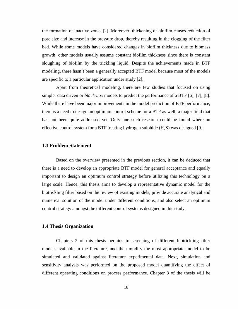
The model considers mass transfer effect at gas-liquid interface, mass transfer
resistance in the liquid phase, variation of liquid film thickness, and velocity distribution
in the liquid and gas regions (Fig. 2-5). Variation in liquid film thickness was considered
in response to the significant effect of mass transfer in liquid layer on VOC removal.
Although equations were derived for changes in liquid film thickness with the height of
the packed bed, the liquid film thickness was eventually concluded to be constant on
account of a fully developed gas flow. Over prediction was observed while comparing
theoretical results with experimental data. It was then proposed that the packing material
was not fully covered with the biofilm, implying that the original area of active biofilm
needed to be modified through a correction factor. With the modified area, the
experimental results were well predicted by the model. Biodegradation in the biofilm
followed Monod and Andrews type kinetics that considers oxygen limitation and
inhibition effects in addition to the substrate (VOC) limitation. The resulting equations
consist of steady state mass balance equations for both VOC and oxygen in the three
phases and momentum balance equations for derivation of the liquid film thickness
profile.
24
Figure 2-5. Schematic of the model structure proposed by Liao et. al [11] under a) co-current and
b) counter-current flows
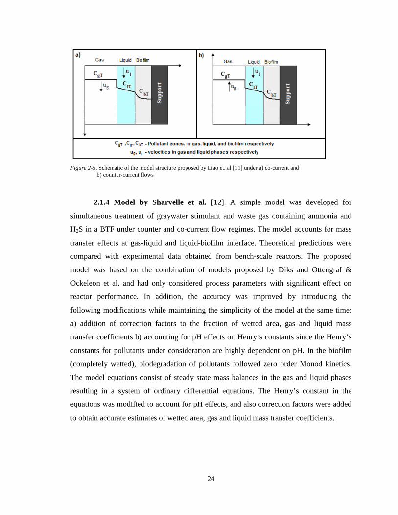
2.1.4 Model by Sharvelle et al. [12]. A simple model was developed for
simultaneous treatment of graywater stimulant and waste gas containing ammonia and
H2S in a BTF under counter and co-current flow regimes. The model accounts for mass
transfer effects at gas-liquid and liquid-biofilm interface. Theoretical predictions were
compared with experimental data obtained from bench-scale reactors. The proposed
model was based on the combination of models proposed by Diks and Ottengraf &
Ockeleon et al. and had only considered process parameters with significant effect on
reactor performance. In addition, the accuracy was improved by introducing the
following modifications while maintaining the simplicity of the model at the same time:
a) addition of correction factors to the fraction of wetted area, gas and liquid mass
transfer coefficients b) accounting for pH effects on Henry’s constants since the Henry’s
constants for pollutants under consideration are highly dependent on pH. In the biofilm
(completely wetted), biodegradation of pollutants followed zero order Monod kinetics.
The model equations consist of steady state mass balances in the gas and liquid phases
resulting in a system of ordinary differential equations. The Henry’s constant in the
equations was modified to account for pH effects, and also correction factors were added
to obtain accurate estimates of wetted area, gas and liquid mass transfer coefficients.

25
2.1.5 Model by Lee & Heber [13]. A genetic algorithm was implemented using a
dynamic model to obtain accurate estimates of process parameters for the removal of
ethylene in a co-current BTF. The model was based on the modified form of the model
proposed by Alonso et al. [10]. Experimental data were used to get optimum values of the
parameters that would result in the least mean square errors between model and
experimental results. Although the pollutant in the gas diffuses into the liquid layer and
then into the biofilm where biodegradation occurs, it was emphasized that the pollutant
transfer through the aqueous layers is affected by its hydrophilicity. A hydrophilic
compound has less resistance to mass flow through the liquid layer than a hydrophobic
compound. Large mass transfer resistance through a thick liquid film prevents transfer of
a hydrophobic compound to the biofilm, resulting in an inactive biofilm. Since the
pollutant under consideration (ethylene) is a hydrophobic compound, it was proposed that
the liquid film thickness could be minimized to the point of being almost non-existent
and that the pollutant in the gas phase is directly transferred to the biofilm (Fig. 2-6). On
the other hand, pollutant removal in the completely non-wetted biofilm is described by
first order Monod kinetics and that there are dynamic changes in biofilm thickness as
well.
Figure 2-6. Concentration gradient of hydrophobic compound without liquid
barrier in the model proposed by Lee and Heber [13]
The model equations consisted of partial differential equations (PDEs) describing
dynamic changes of pollutant concentrations in the gas and biofilm phases. The gas phase
concentration of pollutant varied with time and height of the BTF whereas the

26
concentration of pollutant in the biofilm varied with biofilm depth, height, and time. The
PDEs also included an equation for describing dynamic change in the biofilm thickness.
2.1.6 Summary of models reviewed. A summary of the models reviewed above
is shown in Table 2-1. As shown, there have been some remarkable achievements in the
field of BTF modeling. Most of the models reviewed are similar to each other with
respect to the processes occurring in each of the three phases. It has also been observed
that in most of the VOC removal BTF models, biomass accumulation effect on biofilm
thickness has been considered while for H2S removal process the accumulation effects
have been neglected. This observation has been supported by [5] as well, where it has
been stated that VOC degrading BTFs produce thicker biofilms than H2S degrading
BTFs. Regarding the biodegradation of pollutant in the biofilm, there has been a variation
in the type of kinetics used ranging from the simplest form of Monod kinetics to the more
realistic Andrews type kinetics. The main limitation observed in these models is their
specific applicability towards the pollutant being treated. Thus, there may be
uncertainties in applying a model, specific to one pollutant, over another pollutant [5].
Although coming up with a general BTF model would be a great achievement, this task is
quite challenging and would require considerable effort. One probable cause of facing
such difficulties may be the “difference in process biology” observed between treating
different types of pollutants [5].

27
Table 2-1 Summary of Reviewed Models
Kim & Deshusses [5]
Alonso et al. [10]
Liao et al. [11]
Sharvelle et al. [12]
Lee & Heber [13]
Gas Pollutant (s)
H2S VOC Low conc. VOC
Ammonia H2S
Ethylene
Model Dynamics
Dynamic
Dynamic Steady state Steady state Dynamic
Mode of Operation
Countercurrent Co-current Counter & Co-current
Counter & Co-current
Co-current
Phases Considered
Gas
Liquid
Wetted biofilm
Non-wetted biofilm
Gas
Liquid
Wetted biofilm
Gas
Liquid
Wetted biofilm
Gas
Liquid
Wetted biofilm
Gas
Non-wetted biofilm
Gas Phase Properties
Plug flow
Plug flow
Additional case of axial dispersion for parallel pipes based model
Plug flow Plug flow Plug flow
Biofilm Phase Characteristics
Michelis-Menten kinetics Constant biofilm depth
Monod kinetics Variation in biofilm depth
Monod and Andrews type kinetics Constant biofilm depth
Zero order Monod kinetics Constant biofilm depth
First order Monod kinetics Variation in biofilm depth
Other Characteristics
Conc. varies along bed height and biofilm depth Interfacial mass transfer resistances
Conc. varies along bed height and biofilm depth Three models proposed w.r.t. to packing geometry
Conc. varies along bed height and biofilm depth Considers change in liquid film thickness & incomplete coverage of packing by biofilm
Conc. varies along bed height Added correction factors to mass transfer parameters pH effects considered
Conc. varies along bed height and biofilm depth Considers non-existent liquid layer due to min. trickling liq. rate & hydrophobic pollutant
28
2.2 BTF Model Selection As mentioned earlier, selecting a BTF model is one of the main objectives of this
study. The main aim here was to select a model that would be simple in terms of getting a
mathematical solution while at the same time, it would account for most of the
phenomena occurring in a BTF process. Therefore, the model proposed by Kim &
Deshusses [5] met these objectives and was selected as the target model for performance
prediction and analysis of the BTF process. While the modeling achievements made by
other researchers are worth mentioning, the significant consideration of mass transfer
resistances and additional phase for non-wetted biofilm in the model by [5] is remarkable.
However, the only limitation lies in the type of pollutant being treated. As a result,
hydrogen sulphide (H2S), pollutant of interest in [5], is the target pollutant considered in
this study.
2.3 BTF Model Formulation This section focuses on listing the assumptions and equations used by [5] in
model formulation of H2S abatement in a BTF. Moreover, Kim & Deshusses’ model [5]
was modified to account for continuous and larger BTF system.
2.3.1 Model assumptions. The model had been developed based on the following
assumptions [5]:
1) There is complete coverage of the packing material by the biofilm, which has
uniform thickness. The assumption of a constant biofilm thickness has been
supported by the observation that H2S removing BTFs usually produce thin
biofilms [5].
2) There is presence of both wetted and non-wetted biofilm due to partial wetting of
the biofilm.
3) Dynamic changes in the wetting of the biofilm are not considered.
4) There is no adsorption of contaminant onto the support material

29
5) Plug flow conditions exist in the gas phase. There are no radial changes in
concentration or axial dispersion.
6) Interfacial mass fluxes are expressed by mass transfer coefficients.
7) Gas to liquid and gas to non-wetted biofilm mass transfer coefficients are equal to
each other
8) Gas-liquid, gas-biofilm, and liquid-biofilm interfaces are at equilibrium
9) Diffusion in the biofilm is described by Fick’s law
10) Biodegradation kinetics in the biofilm follow a Michelis-Menten relationship and
H2S is the only rate limiting substrate. Hence, there are no oxygen and nutrient
limitations. Moreover, the biokinetic parameters are same for the wetted and non-
wetted biofilm.
11) No reaction in the liquid phase since there is negligible amount of biomass in the
recycled trickling liquid used in [5].
12) pH effects are neglected since pH had been controlled in the experiment
conducted by [5].
13) Physical properties like temperature, pressure etc. are assumed to be constant.
2.3.2 Model equations. The dynamic model equations consist of mass balances in
each phase, where the height of the BTF and biofilm depth has been discretized into j
(numbered from bottom of the packed bed) and i (numbered from biofilm interface)
segments respectively. Hence, the equations contain finite difference approximations for
changes along the height and biofilm depth, resulting in a system of ordinary differential
equations. For finite differentiation, each subdivision is assumed to be ideally mixed. A
schematic of the resulting model structure is shown in Fig. 2-7.

30
Figure 2-7. Model structure proposed by Kim and Deshusses [5].
Note: Notations given in Nomenclature section
Based on the assumptions, the equations developed by Kim and Deshusses [5] are
as follows:
Gas phase
VgdCg[ j ]
dt= Fg�Cg[ j -1 ] - Cg [ j ]� - kgl Aw�Cg[ j ] – Cgi1[ j ]� - (2.1)
kg2 Anw�Cg[ j ] - Cgi2[ j ]�
Liquid phase
VLdCL[ j ]
dt= FL(CL[ j +1 ] - CL [ j ]) + kgl Aw�Cg[ j ] – Cgi1[ j ]� - (2.2)
kL Aw(CL[ j ] - CLi2[ j ])

31
Non-wetted biofilm phase
− For i =1 (biofilm interface),
dCwb[1 , j]dt
= 𝐷𝐿
�FT2� (CL[ j ] - 2Cwb[1 , j] + Cwb[ 2 , j]) -
Rmax Cwb[1 , j]Ks+ Cwb[1 , j]
(2.3)
− For i = 2 to N -1,
dCwb[i , j]dt
= 𝐷𝐿
�FT2� (Cwb[ i -1 , j] - 2Cwb[i , j]+ Cwb[ i+1 , j]) -
Rmax Cwb[i , j]Ks+ Cwb[i , j]
(2.4)
− For i = N (biofilm depth point),
dCwb[N , j]dt
= 𝐷𝐿
(∆𝐹𝑇)2 (Cwb[ N-1 , j] - Cwb[N , j]) - Rmax Cwb[N , j]Ks+ Cwb[N , j]
(2.5)
Wetted biofilm phase
− For i =1 (biofilm interface),
dCnwb[1 , j]dt
= 𝐷𝐿
(∆𝐹𝑇)2 �Cg[ j ]
H - 2Cnwb[1 , j] + Cnwb[ 2 , j]� -
Rmax Cnwb[1 , j]Ks+ Cnwb[1 , j]
(2.6)

32
− For i = 2 to N -1,
dCnwb[i , j]dt
= 𝐷𝐿
(∆𝐹𝑇)2 (Cnwb[ i -1 , j] – 2Cnwb[i , j]+ Cnwb[ i+1 , j]) (2.7)
- Rmax Cnwb[i , j]Ks+ Cnwb[i , j]
− For i = N (biofilm depth point),
dCnwb[N , j]dt
= 𝐷𝐿
(∆𝐹𝑇)2 (Cnwb[ N-1 , j] - Cnwb[N , j]) - Rmax Cnwb[N , j]Ks+ Cnwb[N , j]
(2.8)
Note: Variable notations have been provided in the Nomenclature section.
Initial conditions
Gas and liquid phases
Cg(1) = Cg0
CL(1) = Cg0H (Henry's law)
Cg(j) = CL(j) = 0, where j ≠1
Wetted and non-wetted biofilm phases
Cwb(1,1)= Cg0H
Cwb(i,j) = 0, where j ≠ 1
Cnwb(i,j) = 0, for all i and j
2.3.3 Modified BTF Model. In the modeling study conducted by [5], the
proposed model was validated with a differential BTF operated in batch mode. This was
done to ease the effort required in the determination of the biodegradation kinetics
parameters and also to reduce the mass transfer resistance in the gas film by operating at
higher gas flows than usual. The model equations for gas phase listed in the previous

33
section account for the gas outlet being continuously recycled to BTF column as the inlet.
In this case, the inlet concentration decreases and depends on the outlet concentration
whereas the inlet concentration to a continuous BTF is usually constant and independent
of outlet concentration. For the purpose of modeling the BTF process in continuous
mode, equation (2.1) was reconstructed as follows:
− For j = 1 (reactor inlet),
Cg(1) = Cg0 (2.9)
− For j = 2 to N (reactor outlet point),
Refer to equation (2.1)
Another issue that needs discussion is the size of the experimental reactor and the
estimated parameters used in the validation experiment conducted by [5]. A differential
reactor had been used and some of the model parameters were experimental. In
particular, the dynamic liquid hold-up (VL) appearing in equation (2.2) was calculated
based on an empirical equation and it is applicable only for the size of the packed bed
considered and not valid for extrapolation [5]. For the control objectives considered in
this study, using a differential BTF would be inappropriate. Moreover, if the BTF is
scaled up, there would be uncertainties in using some of the experiment based model
parameters provided in [5]. Also, determining these parameters using alternative methods
is quite difficult and in some cases impossible without an experiment. To solve this
problem, cascade of n-multistage batch reactors were proposed to represent the
continuous process in the limit as the number of stages goes to a large number n as shown
in Fig. 2-8.

34
Figure 2-8. BTFs in series model structure
With the proposed reactors in series model and in addition to the assumptions
listed earlier, it is assumed that the BTFs connected in series are identical to each other in
terms of size and performance as predicted by Kim & Deshusses’ [5] model. The
required changes in the model equations for the proposed model are as follows:
− For the first reactor, equation (2.9) applies in addition to equations (2.1) – (2.8)
since this represents the inlet point of the scaled-up reactor and has a constant H2S
feed concentration.
− For second to nth reactor, only equations (2.1) to (2.8) apply since the inlet
concentration to each of these reactors is changing. This is due to the fact that the
outlet of one reactor serves as an input to the other reactor that follows it in series
and the outlet concentration is changing with time.
35
2.4 Model Simulation This section provides a dynamic analysis of the BTF performance through
simulation of the model formulated in the previous sections. Both Kim and Deshusses’
original model [5] and the modified model proposed in this work will be simulated.
Sensitivity analysis of the important process parameters using steady state outlet
concentration of H2S as the BTF performance indicator has also been performed.
However, the dynamic analysis will be based on simulation of the modified model only.
Kim and Deshusses’ model will be simulated only for the purpose of comparing the
results with those obtained in [5] and also to verify its validity with experimental data.
All the required simulations were carried out using MATLAB R2009b numerical solver
for ODEs. MATLAB codes are given in the Appendix. Moreover, the simulations were
run on an Intel Core 2 Duo T5800 2.00 GHz processor.
2.4.1 BTF process conditions and model parameters. In the validation
experiment conducted by [5], the packed bed consisted of a single cube of open pore
polyurethane foam (PUF) with the gas and the trickling liquid being continuously
circulated through the differential BTF in batch mode. Further details about the
experiment can be found in [5]. The BTF system properties and conditions used for
model simulations and analyses are shown in Table 2-2. The height of the BTF required
for scale-up was fixed and determined according to the removal efficiency of the original
differential BTF in [5]. In other words, the height was adjusted until the removal
efficiency in the scaled-up BTF was approximately the same as that observed in the
differential BTF. Hence, according to the BTFs in series model, the resulting pilot scale
BTF required forty differential BTFs in series.
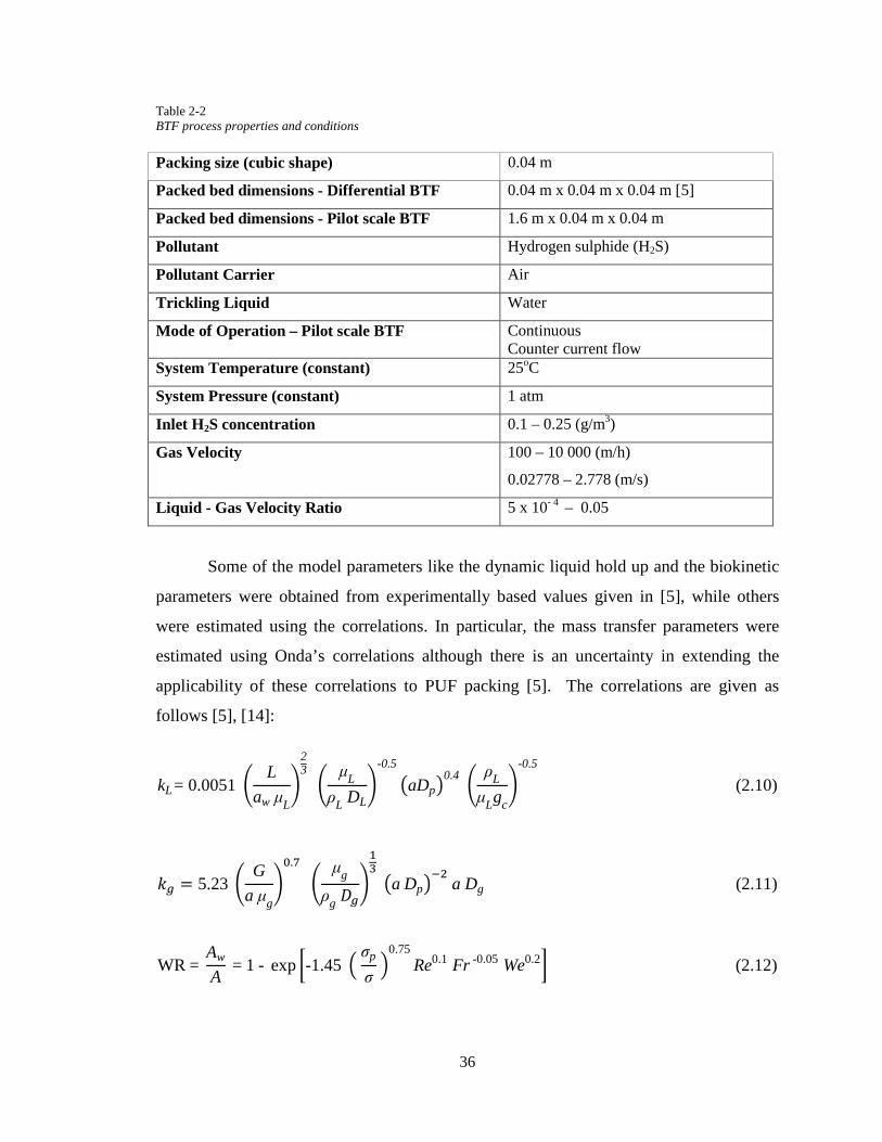
36
Table 2-2 BTF process properties and conditions Packing size (cubic shape) 0.04 m
Packed bed dimensions - Differential BTF 0.04 m x 0.04 m x 0.04 m [5]
Packed bed dimensions - Pilot scale BTF 1.6 m x 0.04 m x 0.04 m
Pollutant Hydrogen sulphide (H2S)
Pollutant Carrier Air
Trickling Liquid Water
Mode of Operation – Pilot scale BTF Continuous Counter current flow
System Temperature (constant) 25oC
System Pressure (constant) 1 atm
Inlet H2S concentration 0.1 – 0.25 (g/m3)
Gas Velocity 100 – 10 000 (m/h)
0.02778 – 2.778 (m/s)
Liquid - Gas Velocity Ratio 5 x 10- 4 – 0.05
Some of the model parameters like the dynamic liquid hold up and the biokinetic
parameters were obtained from experimentally based values given in [5], while others
were estimated using the correlations. In particular, the mass transfer parameters were
estimated using Onda’s correlations although there is an uncertainty in extending the
applicability of these correlations to PUF packing [5]. The correlations are given as
follows [5], [14]:
kL= 0.0051 �L
aw μL�
23
�μL
ρL DL�
-0.5
�aDp�0.4
�ρLμLgc
�-0.5
(2.10)
𝑘𝑔 = 5.23 �G
a μg�0.7
�μg
ρg 𝐷𝑔�
13
�a Dp�−2
a Dg (2.11)
WR = Aw
A = 1 - exp �-1.45 �
σp
σ �
0.75Re0.1 Fr -0.05 We0.2� (2.12)

37
A summary of the model parameters used excluding the system conditions is
shown in Table 2-3. Since the value of gas hold up had not been mentioned in [5], it was
estimated using a simple expression (shown in Table 2-3) involving an approximated gas-
liquid volume ratio and liquid hold up.
Table 2-3 BTF model parameters
Parameter Value/Equation Calculation Method/ Reference
kg (gas-liq. mass transfer coefficient) Equation (2.10) Onda’s correlation [5], [14]
kL (liq. -biofilm mass transfer coefficient) Equation (2.11) Onda’s correlation [5], [14]
FT (biofilm thickness) 23 μm [5]
Rm (maximum reaction rate) 58 400 g/(m3.h) Experiment based value [5]
KS (Michaelis-Menten constant) 0.0279 g/m3 Experiment based value [5]
H (Henry’s constant for H2S) 0.387 [5]
DL (diffusion coefficient of H2S in liq.) 5.796 x 10⁻⁶ m2/h [5]
Dg (diffusion coefficient of H2S in air) 1.6332 x 10⁻² m2/h Fuller correlation [15]
a (specific interfacial area) 600 m2/m3 [5]
VL (dynamic liquid holdup) (1 x 10⁻⁵)FL + (8 x 10⁻⁶) Experimental correlation [5]
Vg/L (gas-liquid volume ratio) 8.6 x 10⁴ Approximation based on experimental conditions in [5]
Vg (gas volume/gas hold up) Vg/L * VL Estimation
i,j (discretized segments along biofilm depth and BTF height respectively)
10 [5]
In [5], the model results were validated with experimental data at certain process
conditions. These conditions (shown in Table 2-4) have been considered as the base
conditions and the term will be used wherever the use of these conditions is required in
the upcoming discussions.
Table 2-4 Base conditions for BTF process
Variable Value
Inlet concentration of H2S (g/m3) 0.164
Gas velocity (m/h) 9 400
Liquid-gas velocity ratio 1.2553 x 10- 3
38
2.4.2 Solution Methodology. The simulation of the model required for analyses
was performed using MATLAB R2009b. The original Kim and Deshusses’ model [5]
involving system of stiff ordinary differential equations (ODEs) was solved using the
ode15s solver in MATLAB. The ode15s is a multistep solver based on numerical
differentiation formulae (NDF) and is used for solving stiff initial value problems for
ODEs [16]. In case of the proposed model, a different solution methodology was applied
before solving the model equations in MATLAB. Solving the ODEs for each of the forty
reactors in series in MATLAB would require tremendous computational effort and time,
making this solution methodology an unfeasible technique for simulation of the proposed
model. Hence, a pseudo-steady state assumption was applied while simulating the
proposed model where all the reactors in series except the first are simulated at steady
state. For the first reactor, the equations are solved using the ODE solver in MATLAB
similar to the solution of the original model. This numerical solution generates H2S
concentrations at each of the discretized time elements. At each discretized time, the
outlet concentrations are input as the inlet concentrations to the second reactor. In
addition, the model equations are solved assuming steady state condition at each
discretized time (Fig. 2-9). Finally, the steady state concentrations at all time elements are
compiled together to obtain a time dependent concentration profile for the second reactor.
This algorithm is repeated for all the remaining reactors to obtain the outlet concentration
profile for the pilot scale BTF overall. Hence, a program was created in MATLAB to
perform these computations for the proposed model scheme. In case of model sensitivity
analysis, the model equations for all the reactors were solved at steady state conditions
since the analyses had been performed based on the effect of process parameters on
steady state outlet concentration. The system of non-linear equations resulting from the
steady state assumption of the model equations was solved using the fsolve command
in MATLAB that uses the trust-region dogleg method of solution for non-linear
equations [17].

39
Figure 2-9. Solution scheme for BTFs in series model
2.4.3 Results and discussion 2.4.3.1 Simulation and validity of original model. The simulated concentration
profiles at the inlet of the differential BTF including the experimental data obtained
from [5] are shown in Fig. 2-10. The CPU time for this simulation was around
53 seconds. The original model was simulated at the base gas and liquid flows with
concentration profiles obtained at both high and low initial inlet H2S concentrations. As
expected, both the profiles show a non-linear decrease in inlet H2S concentration with
time since the pollutant (H2S) is continuously being removed by mass transfer and
biodegraded by the micro-organisms during circulation of the gas through the batch
reactor. At the end of the simulation time, approximately 94 percent H2S removal
efficiency had been achieved. The profiles in Fig. 2-10 also include the original model
solution by Kim and Deshusses [5]. It can be clearly seen that the original model profiles
from [5] have been successfully reproduced by the model solution in this work as both
the profiles are mostly close to each other. Overall, it can be observed that the model
agrees well with experimental data at high initial H2S concentration whereas over
prediction exists at lower concentration. Through sensitivity analysis of nine model
parameters and examination of concentration profiles in the biofilm at low H2S

40
concentration, [5] deduced that there had been mass transfer limitation in the biofilm
resulting in the formation of inactive biofilm zones. It was also observed that the
accuracy of model prediction at lower concentration improved after changing the value of
H2S diffusivity in liquid [5]. The exact justification for this behavior could not be figured
out, but was explained to be probably related to inaccuracies in model parameters [5].
Nevertheless, changes to the H2S diffusivity were unnecessary for this study since the
inlet H2S concentrations considered for simulations ranged from intermediate to high
levels. Hence, the model proves to be sufficiently reliable for the range of the inlet
concentrations considered without the need of modification to H2S diffusivity.
Figure 2-10. Comparisons between original model predictions and experimental data.
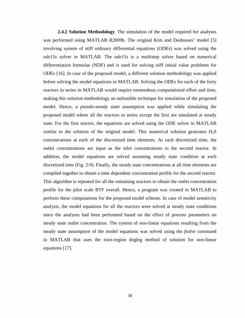
2.4.3.2 Simulation of the modified model. Analogous to the dynamic batch
concentration profiles in Fig. 2-10, the steady state concentration profile at the base
conditions along the length (or number of differential BTFs) of the continuous pilot scale
BTF is shown in Fig. 2-11. A similar non-linear behavior is observed where the steady
state H2S concentration continuously decreases as the gas flows through the length of the
BTF column. It can also be deduced that more H2S could be treated by increasing the
height of packed bed. Since the size of pilot scale BTF had been adjusted according to the
41
performance of the batch BTF in [5] at the base conditions, overall H2S removal
efficiency of approximately 94 % had been observed with the modified model simulation.
Figure 2-11. Simulation of the proposed BTFs in series model at steady state
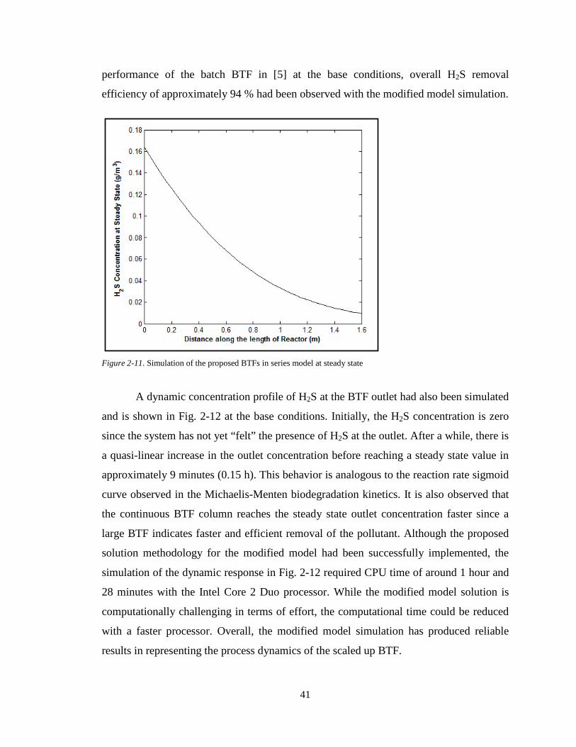
A dynamic concentration profile of H2S at the BTF outlet had also been simulated
and is shown in Fig. 2-12 at the base conditions. Initially, the H2S concentration is zero
since the system has not yet “felt” the presence of H2S at the outlet. After a while, there is
a quasi-linear increase in the outlet concentration before reaching a steady state value in
approximately 9 minutes (0.15 h). This behavior is analogous to the reaction rate sigmoid
curve observed in the Michaelis-Menten biodegradation kinetics. It is also observed that
the continuous BTF column reaches the steady state outlet concentration faster since a
large BTF indicates faster and efficient removal of the pollutant. Although the proposed
solution methodology for the modified model had been successfully implemented, the
simulation of the dynamic response in Fig. 2-12 required CPU time of around 1 hour and
28 minutes with the Intel Core 2 Duo processor. While the modified model solution is
computationally challenging in terms of effort, the computational time could be reduced
with a faster processor. Overall, the modified model simulation has produced reliable
results in representing the process dynamics of the scaled up BTF.
42
Figure 2-12. Dynamic simulation of the proposed BTFs in series model
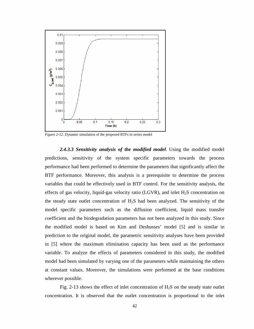
2.4.3.3 Sensitivity analysis of the modified model. Using the modified model
predictions, sensitivity of the system specific parameters towards the process
performance had been performed to determine the parameters that significantly affect the
BTF performance. Moreover, this analysis is a prerequisite to determine the process
variables that could be effectively used in BTF control. For the sensitivity analysis, the
effects of gas velocity, liquid-gas velocity ratio (LGVR), and inlet H2S concentration on
the steady state outlet concentration of H2S had been analyzed. The sensitivity of the
model specific parameters such as the diffusion coefficient, liquid mass transfer
coefficient and the biodegradation parameters has not been analyzed in this study. Since
the modified model is based on Kim and Deshusses’ model [5] and is similar in
prediction to the original model, the parametric sensitivity analyses have been provided
in [5] where the maximum elimination capacity has been used as the performance
variable. To analyze the effects of parameters considered in this study, the modified
model had been simulated by varying one of the parameters while maintaining the others
at constant values. Moreover, the simulations were performed at the base conditions
wherever possible.
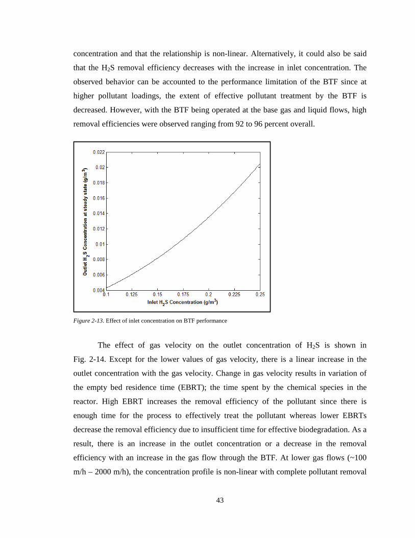
Fig. 2-13 shows the effect of inlet concentration of H2S on the steady state outlet
concentration. It is observed that the outlet concentration is proportional to the inlet
43
concentration and that the relationship is non-linear. Alternatively, it could also be said
that the H2S removal efficiency decreases with the increase in inlet concentration. The
observed behavior can be accounted to the performance limitation of the BTF since at
higher pollutant loadings, the extent of effective pollutant treatment by the BTF is
decreased. However, with the BTF being operated at the base gas and liquid flows, high
removal efficiencies were observed ranging from 92 to 96 percent overall.
Figure 2-13. Effect of inlet concentration on BTF performance
The effect of gas velocity on the outlet concentration of H2S is shown in
Fig. 2-14. Except for the lower values of gas velocity, there is a linear increase in the
outlet concentration with the gas velocity. Change in gas velocity results in variation of
the empty bed residence time (EBRT); the time spent by the chemical species in the
reactor. High EBRT increases the removal efficiency of the pollutant since there is
enough time for the process to effectively treat the pollutant whereas lower EBRTs
decrease the removal efficiency due to insufficient time for effective biodegradation. As a
result, there is an increase in the outlet concentration or a decrease in the removal
efficiency with an increase in the gas flow through the BTF. At lower gas flows (~100
m/h – 2000 m/h), the concentration profile is non-linear with complete pollutant removal

44
observed at very low gas flows (~ 100m/h – 500 m/h). Hence, the pollutant removal
efficiency of a BTF could be improved by decreasing the gas velocity, but only to a
certain extent since gas phase mass transfer resistances increase at lower gas flows.
Figure 2-14. Effect of gas velocity on BTF performance
Finally, the effect of liquid-gas velocity ratio (or the liquid velocity in other
words) at the base inlet concentration and gas velocity is shown in Fig. 2-15.
Interestingly, a parabolic relationship is observed between the steady state outlet
concentration and liquid-gas velocity ratio (LGVR) where the outlet concentration
initially increases with the LGVR until reaching a maximum value and decreasing with
further increase in LGVR. It can be observed that apart from the maximum point, two
LGVR values exist for the same outlet concentration. This behavior is indicative of the
mass transfer limitations in the liquid phase since a change in LGVR causes a change in
the liquid velocity which in turn affects the thickness of the liquid layer surrounding the
wetted biofilm. At very low values of LGVR (low liquid velocity), the removal efficiency
is high (low outlet concentration) since the hydrodynamic layer is almost non-existent
and offers very less resistance to mass flow of the pollutant to the biofilm. As the LGVR
increases, the addition of a liquid layer increases the mass transfer resistance resulting in
the increase of outlet concentration or decrease in removal efficiency. In fact, while

45
performing a trial simulation of the original model with the assumption of a completely
wetted biofilm, it had been observed that the removal efficiency at the end of the
simulation time (2 hours) was very low. The increase in the removal efficiency beyond
the minimum point (maximum point in case of outlet concentration) can be related to the
decrease in the hydrodynamic layer at higher LGVR values. In other words, the liquid
velocity is now sufficiently large to cause a decrease in the hydrodynamic layer and also
a decrease in the mass transfer resistance as a result. Looking at the trend of the
concentration profile, it is expected that beyond the maximum limit of the LGVR
considered in this study, the outlet concentration would eventually reach a constant value,
implying that the removal process is now limited to diffusion and biodegradation in the
biofilm and that the outlet concentration is no longer affected by higher values of LGVR.
In general, it can be deduced that BTFs can be operated at lower trickling liquid rates and
also, that the performance of a BTF is not strongly affected by the trickling liquid.
Figure 2-15. Effect of liquid-gas velocity ratio on BTF performance
Based on the sensitivity analysis of the physical process parameters, it can be
concluded that the inlet concentration of H2S and the gas velocity are the most significant
variables affecting the performance of the BTF and that the performance is only affected

46
at very small range of LGVR. Hence, the LGVR can be considered as a constant and
optimized to achieve an efficient performance overall. These conclusions would be
helpful in designing and implementing an efficient control strategy for the BTF; a major
part of this study that will discussed in the next chapter.

47
Chapter 3. Biotrickling Filter System Identification and Control
Designing an optimum control system is one of the most essential phases during
the implementation of any pollutant treatment process. Complying with environmental
regulations and meeting the legal pollutant release limits are the primary reasons of
designing efficient control systems for such processes. However, without accurate
understanding of the process dynamics, designing and effectively implementing control
strategies is impossible. Hence, it is essential that accurate and reliable model
identification of the process dynamics is obtained before implementing any control
strategy. Moreover, it is also important that simulation of the identified model requires
less computational effort and time. This chapter focuses on identifying the BTF process
with simpler and reliable data-driven models followed by proposition of some classical
and advanced control strategies. Through analyses of alternative control strategies
developed in this work, an optimum control strategy will also be determined. Although
the modified model proposed in section 2.3.3 could successfully represent the BTF
process, simulation still requires some computational effort and time. Hence, control
strategies have been based on data-driven models of the BTF. Nevertheless, these black
box models have been fitted with data generated from simulation of the modified model.
Two empirical models have been obtained for the BTF process: 1) step response model
and 2) neural network model.
3.1 BTF System Identification
In general, models developed for identification of process dynamics can be
classified into the following types [18]:
1) Theoretical models: these are first-principles models built upon fundamental laws
of science and simplifying assumptions [19]. Although they provide “physical
insight into process behavior”, they are time-consuming and require parameters that
may not be readily available [18].
2) Empirical or black-box models: these are experimentally-fitted models and are
more easily developed than theoretical models. Moreover, they require less

48
computational effort and time when compared to theoretical models. However, they
have higher certainties of being unreliable for extrapolation [18].
3) Semi-empirical models: these widely used models are combination of theoretical
and empirical models. They offer combined advantages of incorporating theory,
being safe in terms of their use for extrapolation, and requiring less development
effort [18].
In case of designing efficient control systems for complex processes, acquiring
empirical models is more feasible than theoretical models [18]. Several techniques for
experimental identification of process dynamics exist in literature ranging from simplest
models like linear and nonlinear autoregressive exogenous (ARX) models, step response
models to more advanced models like state space models, state estimators or soft sensors,
and the widely known artificial neural network (ANN) models [18], [19], [20]. While the
models are usually developed in continuous form, some of these models have been
developed in discrete form and are applied in cases when the sampling data exist in
discrete form.
Besides the presence of several theoretical BTF models in literature, some studies
have successfully developed empirical models specific to the experimental BTFs under
consideration. In a study conducted by [6], a simple second-order empirical model was
developed for an experimental anoxic BTF treating H2S in biogas. The model had been
successfully developed to predict BTF performance parameters namely H2S removal
efficiency and loading rate using H2S inlet concentration and biogas flow rate as the
inputs. In another study [8], ANN models were developed for three different fungal
bioreactors treating gas phase styrene. The models were developed for three different
bioreactor configurations: 1) biofilter, 2) continuous stirred tank reactor, and 3) monolith
bioreactor also commonly known as BTF [8]. In case of the monolith bioreactor, the
ANN model was used to predict styrene removal efficiency (performance parameter)
using inlet concentration of styrene, gas-liquid flow rate ratio, and pressure drop as the
inputs. Moreover, the ANN parameters were optimized to obtain an optimum value of the
regression coefficient (R2) between experimental and predicted results. Finally, ANN has
also been used in another study [7], where a back-propagation neural network (NN)
model had been successfully developed to predict the performance (elimination capacity

49
and removal efficiency) of a laboratory-scale BTF treating benzene, toluene, and xylene
compounds.
In this work, two data-driven BTF models have been developed prior to the
design and analyses of different control systems: 1) dynamic step response or transfer
function model and 2) steady state NN model. The models are based on data generated
from simulation of the modified model and will predict the outlet concentration of H2S,
selected as the BTF performance criterion, using the inputs discussed in the next section.
3.1.1 BTF input-output structure. In section 2.4.3.3, it had been concluded that
the inlet concentration of H2S and gas velocity were the most influential parameters
affecting BTF performance while LGVR effects were significant only for a small range.
These observations are necessary to list the sufficient number of inputs and outputs for
system identification of the process. In addition, these observations would aid in
proposing a control structure for the BTF process. Hence, the set of input-output
variables used in developing data-driven BTF models is shown in Fig. 3-1. For more
accurate identification of the BTF process with the NN model, LGVR and liquid velocity
have also been used as the inputs. It should also be noted that the liquid velocity input
depends on LGVR and gas velocity by the following relationship:
uL= UL/g . ug (3.1)
On the other hand, transfer function models of the BTF process will be based only
on the first two inputs shown in Fig. 3-1 while maintaining the LGVR at the base values.
Figure 3-1. Input/output structure for system identification of the BTF process

50
3.1.2 Open loop step response models. Fitting a model to step response data is
the most direct method of system identification of a process [20]. This method involves
creating a step change in one of the desired inputs and recording the corresponding output
behavior as a function of time [20]. Once the data has been collected, an appropriate
transfer function (TF) is fitted. Besides step function, the input change could also be in
the form of a pulse signal, sine wave, saw-toothed signal or any arbitrary shaped
signal [18]. Depending on the degree of accurate process representation, the fitted
functions, in Laplace domain, can be either first- or higher-order models. These models
are mainly represented by gain (K), time constant or lag time (𝜏), and sometimes time
delay (𝜃) parameters. Process gain represents ratio of steady state change in the output
over the step change in input whereas time constant provides an insight to the time taken
by the process to reach steady state [20]. Finally, some processes exhibit delays in
changes to output when disturbed by input changes. Hence, this behavior can be
represented in the TF models with time delay terms. Most of the chemical engineering
open loop processes are modeled with first order transfer function models having the
following general form [20]:
G(s) = 𝑌(𝑠)𝑈(𝑠)
= K e -θ s τs + 1 (3.2)
The parameters required for the TF models can be easily determined by graphical
or non-linear regression methods [18]. For the BTF process considered in this work, first
order TF models were obtained to predict the relationship between outlet concentration of
H2S and the two inputs: 1) inlet concentration of H2S, Cg0 and 2) gas velocity, ug. The
input-output dynamic data obtained from simulation of the modified model consisted of
two sets. First, the modified model was simulated to obtain dynamic response of the
outlet concentration at varying gas velocities while maintaining the other input (inlet
concentration) at the base condition. The simulation was repeated with the inlet
concentration being varied at the constant base gas velocity. The input changes were in
step form and were within the operating ranges shown in Table 2-2. While fitting the TF
models, the LGVR was maintained at the base value for the entire simulations. The
51
overall equation for predicting outlet concentration consists of two TF models that are
added together by the superposition principle stated as follows:
𝑌(s) = � GK(s)2
K = 1
UK(s) (3.3)
Each of the two terms in the overall equation represents relationship between
output (outlet concentration) and one of the inputs with no change in the other input. To
develop this equation, it was necessary to transform the data into deviation form given as
follows:
∆X = X - Xnm (3.4)
This transformation ensures that while fitting the model between output and one
of the inputs, the other input has a numeric value of zero. The required nominal values in
equation (3.4) for the inputs were defined at the base conditions whereas the nominal
value of the output was defined to be the steady state output resulting from modified
model simulation at the base conditions. The required parameters for fitting the two TF
models were obtained from the Design Tools Module in Loop Pro Trainer 5.1
software [21]. Each of the two sets of input-output data was entered in this software, a
suitable fitting model from the available models was selected and the final results were
obtained that includes plots, fitted parameters, and the resulting R2 values. The fitted TF
model output results from Loop Pro software were recorded and compared with the
modified model simulation using MATLAB.
3.1.3 Neural network model. Artificial neural network (ANN) models are non-
linear empirical models that have increasingly become important nowadays for modeling
environmental systems [22]. The ANN concept was based on the operation of the human
brain where substantial parallel computations are performed using “structural constituents
called neurons and the synaptic interconnections between them”, thereby creating a
neural network [18]. Likewise, NN computation structure consists of a network of
interconnected neurons organized in layers [18] and it involves using a series of
equations that “stimulate learning and memorization process” [8]. Fitting a neural
52
network model consists of two phases: 1) training phase where the model normally
requires large data sets to estimate the unknown fitting parameters 2) validation and
testing phase where the model uses another set of data to validate and test the trained
network [18]. NN models are useful in modeling non-linear complex processes and also
in replacing models that require significant computational effort and time [18]. Moreover,
ANNs have the advantages of being simple, noise and fault tolerant, and versatile to
process changes [8]. However, ANNs have some disadvantages as well: 1) they require
large data sets for process identification, 2) there is a possibility of over-fitness of the
model with the data, 3) determining network topology for the model by trial and error
can be an intensive task, and 5) the model needs to be re-trained whenever data set is
updated [8].
Depending on the nature of signal transmission between the neurons, NN models
are categorized into two types: 1) feed-forward neural network (FNN) and 2) recurrent
neural network (RNN) models [23]. RNN models consist of networks with both forward
and backward or feedback connections and they are particularly useful in modeling
dynamic systems [23]. FNNs or multilayer perceptrons (MLPs) [23], the model of
interest in this paper, is the commonly used model where signal is transmitted in the
forward direction. In this model, neurons, also known as processing elements (PEs), are
organized into three main layers: 1) an input layer, 2) one or more hidden layers, and 3)
an output layer [22]. At each PE in the hidden layer, inputs (xi) from the preceding layer
are weighted with adjustable connection weights (wij) , added to a threshold value (𝜃𝑗),
combined into an input signal ( Ij ) and finally converted to the output neurons through an
activation function ( f(Ij) ), as shown in Fig. 3-2. For optimization of the connection
weights, there are many training algorithms available in literature some of which include
the widely known back-propagation techniques like Levenberg-Marquardt, Shanno and
conjugate gradient algorithms and global techniques like annealing and genetic
algorithms [22]. In back-propagation FNN, input signals are transmitted in the forward
direction while the error (between measured and predicted values) signals are transmitted
backwards to re-adjust the connection weights accordingly [23]. This process continues
until a best fit NN model is obtained. The most common activation function used in the
FNNs is the logistic sigmoid function that has minimum and maximum values of 0 and 1

53
respectively [8]. Other activation functions include hyperbolic tangent, polynomial,
rational functions and Fourier series [8]. Due to the nature of the activation functions, the
measured data set needs to be normalized to fall within the range of these functions.
Finally, determining the network topology, i.e. the optimum number of neurons in each
layer, is the most important task that determines how well the model fits to the process
data. The number of neurons in the input and output layers is equal to the number of
process inputs and outputs. Although there are some heuristics that help in estimating the
number neurons in the hidden layer, this task is usually accomplished by trial and error.
Figure 3-2. General FNN structure [22]
For modeling the BTF process with NNs, four inputs and one output, shown in
Fig. 3-1, were used. A steady state NN model was obtained using the data from
simulation of the modified model at steady state. The NN model was obtained using the
Neural Network Fitting Tool in MATLAB R2009b. This tool uses two-layer FNN with
log sigmoid function for the hidden layer neurons and a linear function for the output
layer neurons. Moreover, this tool trains the network using Levenberg-Marquardt back-
propagation algorithm. Due to the limits of the activation function, the input data was
normalized using the following expression [8]:
Xn = X - Xmin
Xmax - Xmin (3.5)

54
Since the output data fall within the limits of the activation function, the output
data was not normalized. Moreover, the percentages of overall data used for training,
validating, and testing the NN model were 70, 20, and 10 respectively. The transformed
steady state input-output data from the modified model simulation were entered into the
NN fitting tool, an optimum network topology was determined through trial-and-error
and the resulting best fitted NN model was finally obtained. The overall results included
comparisons, error and R2 value between NN model predictions and data. As a final step,
the fitted NN model was simulated to analyze the output response with a step change in
gas velocity and inlet concentration. Moreover, the output results were compared with
those obtained from the modified model. The NN model obtained from the NN Fitting
Tool was embedded and simulated in Simulink; an add-on software in MATLAB used to
model, simulate, and analyze dynamic systems. The simulation results from Simulink
were recorded and compared with the modified model using MATLAB. The Simulink
block diagram for the NN model simulation is provided in the Appendix.
3.1.4 Results and discussion
3.1.4.1 Identified transfer function BTF models. The fitted TF model predictions
of outlet concentration in response to step changes in gas velocity are compared with the
modified model simulations and shown in Fig. 3-3. The input and output values represent
deviation from the nominal values i.e. the base conditions. Since the values of the input
and output in deviation form are considered to be zero at the base conditions, the negative
and positive values represent negative and positive deviations from the base conditions
respectively. In case of the output (outlet concentration), the base value represents the
outlet concentration resulting from modified model simulation at the base conditions.
Hence, the negative output values in Fig. 3-3 denote that the outlet concentration has
decreased relative to the base value meaning that the removal efficiency has increased
relative to the base removal efficiency (94%). Before commenting on the TF model
representation of the BTF, some observations can be made on dynamic response of the
output (outlet concentration) with respect to step changes in gas velocity. Almost all of
the step changes in gas velocity cause similar step changes in the output. This implies that
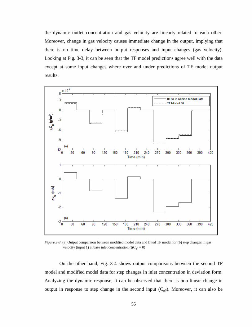
55
the dynamic outlet concentration and gas velocity are linearly related to each other.
Moreover, change in gas velocity causes immediate change in the output, implying that
there is no time delay between output responses and input changes (gas velocity).
Looking at Fig. 3-3, it can be seen that the TF model predictions agree well with the data
except at some input changes where over and under predictions of TF model output
results.
Figure 3-3. (a) Output comparison between modified model data and fitted TF model for (b) step changes in gas velocity (input 1) at base inlet concentration (𝚫Cg0 = 0)
On the other hand, Fig. 3-4 shows output comparisons between the second TF
model and modified model data for step changes in inlet concentration in deviation form.
Analyzing the dynamic response, it can be observed that there is non-linear change in
output in response to step change in the second input (Cg0). Moreover, it can also be
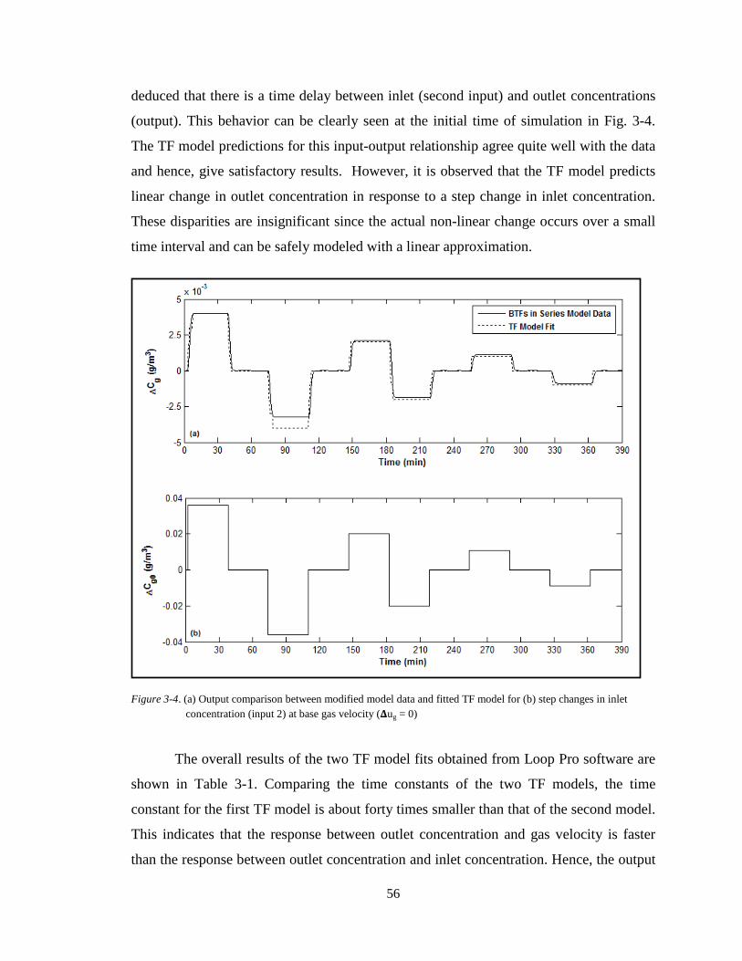
56
deduced that there is a time delay between inlet (second input) and outlet concentrations
(output). This behavior can be clearly seen at the initial time of simulation in Fig. 3-4.
The TF model predictions for this input-output relationship agree quite well with the data
and hence, give satisfactory results. However, it is observed that the TF model predicts
linear change in outlet concentration in response to a step change in inlet concentration.
These disparities are insignificant since the actual non-linear change occurs over a small
time interval and can be safely modeled with a linear approximation.
Figure 3-4. (a) Output comparison between modified model data and fitted TF model for (b) step changes in inlet concentration (input 2) at base gas velocity (𝚫ug = 0)
The overall results of the two TF model fits obtained from Loop Pro software are
shown in Table 3-1. Comparing the time constants of the two TF models, the time
constant for the first TF model is about forty times smaller than that of the second model.
This indicates that the response between outlet concentration and gas velocity is faster
than the response between outlet concentration and inlet concentration. Hence, the output

57
(outlet concentration) will reach a new steady state much faster with change in gas
velocity than the inlet concentration. Looking at the time delays, there is also an
approximately 1 minute time delay between output and input changes for the second
model whereas the first model has no time delay. These results indicate that the dynamic
behavior of the output in response to inlet concentration is quite slow and that changes in
inlet concentration will have a major effect on optimization of BTF process performance
and control. Finally, the values of R2 and sum of squares for error (SSE) prove that both
the TF models are collectively reliable in predicting the BTF performance overall. The
overall transfer function BTF model for predicting the outlet concentration can now be
formulated in deviation form as follows:
Δ𝐶𝑔 (s) = 4.388 x 10⁻³
(1.8s + 1) Δ𝑢𝑔 (s) + 0.1007 e-54s
(72.57s + 1) Δ𝐶𝑔0 (s) (3.6)
Table 3-1 Results summary of fitted BTF transfer function models
TF Model 1 G1 (s)
TF Model 2 G2 (s)
Input Δug (m/s) ΔCg0 (g/m3)
Output ΔCg (g/m3) ΔCg (g/m3)
Gain, K 4.388 x 10- 3 �g/m3
m/s� 0.1007 ( - )
Time constant, τ 1.8 s 72.57 s
Time delay, θ 0 54 s
R2 value 0.9824 0.9701
SSE 4.11 x 10⁻⁴ 1.28 x 10⁻⁴

58
3.1.4.2 BTF neural network model identification and simulation. Table 3-2
shows the overall summary of the fitted NN model obtained from NN Fitting Tool. The
optimum network topology was found to be 4 - 7 - 1. In other words, while the number of
neurons in the input and output layers were equal to the number of inputs and output used
for the BTF process, the optimum number of neurons in the hidden layer was found to be
seven through trial and error. As evident from the R2 and mean squared error (MSE)
values, perfect NN model fit of the BTF process had been obtained. Hence, the NN
model proves to be very reliable in predicting steady sate BTF performance. The ability
of the NN model to accurately represent the BTF process can also be attributed to
uncomplicated nature of the process itself where the simple relationships between inputs
and the output can be easily modeled.
Table 3-2 Summary of fitted BTF neural network model
Properties
Inputs
ugn
Cg0n
UL/g n
uLn
Output Cg (g/m3)
Total number of data samples 483
Number of training samples
Number of validation samples
Number of test samples
338
97
48
Results Network topology (Input - hidden - output)
4 - 7 - 1
MSEs
Training
Validation
Test
1.12 x 10⁻¹¹
1.24 x 10⁻¹¹
6.14 x 10⁻¹²
R2 values
Training
Validation
Test
1
1
1

59
The dynamic response of the NN and modified models for a 32 % step decrease in
gas velocity from base value is shown in Fig. 3-5. Although NN model is based on steady
state data, it is observed that the NN model predictions almost perfectly agree with the
modified model dynamic results. The NN model predictions are accurate because
according to the dynamic response shown in Fig. 3-3 earlier, the output (outlet
concentration) immediately reaches steady state value in response to a change in gas
velocity.
Figure 3-5. (a) Output comparison between modified model data and NN model for (b) step
change in gas velocity at base inlet concentration

60
In response to a 12 % step increase in the inlet concentration from the base value,
the dynamic output comparisons between the NN model and the modified model are
shown in Fig. 3-6. Since the steady state NN model does not account for time delay
between output and inlet concentration, a time delay term was included in the Simulink
block diagram. Comparing the predictions between the two models, it is clearly observed
that NN model does not capture the dynamic response observed in the modified model
output observed between 10 and 15 minutes. This discrepancy between the two models is
due to the fact that NN model was derived based on the steady state data. However, the
NN model was able to accurately capture the final steady state values of the modified
model responses.
Figure 3-6. (a) Output comparison between modified model data and NN model
for (b) step change in inlet concentration at base gas velocity

61
To sum up the discussion on system identification of the BTF process, TF and NN
model representations of the BTF were successfully obtained. Overall, the agreement of
dynamic responses from both the fitted models with the modified model data was
satisfactory. With the BTF system being adequately described using simpler
identification models obtained in this section, different control strategies based on these
models will be proposed and implemented in the upcoming sections.

62
3.2 BTF Process Control
With process control, the goal of safely and efficiently maintaining a process at
the desired conditions can be achieved [18]. For treatment processes, designing efficient
control systems is necessary to comply with environmental regulations. To develop an
effective control system, it is essential that the following characteristic process variables
are specified first [18]:
1) Controlled variables (CVs): these are the variables that require to be maintained at
the desired values or set points [18]. In chemical processes, typical control variables
include compositions, flow rates, levels, pressures and temperatures [20].
2) Manipulated variables (MVs): these are the variables adjusted to maintain the
control variables at their set points. Flow rates of entering or leaving streams are the
most common manipulated variables [20].
3) Disturbance variables (DVs): these variables affect the controlled variables and
cannot be freely manipulated [18] since they are usually dependent on the upstream
or downstream conditions of the plant [20]. An efficient control system must be
robust towards preventing process disturbances as much as possible.
In general, control system design has either traditional or model-based
approach [18]. In traditional approach, the control system is implemented only after
major part of the plant design has been completed [18]. The second approach involves
developing a process model first that would be helpful in: 1) forming a basis for model-
based control strategies, 2) being directly integrated into the control law, and 3) being
used in computer simulations for analyzing different control strategies and also in
determining preliminary controller settings, an activity more commonly known as
controller tuning [18]. For simple processes, traditional approach is adequate while the
control system design must be model-based in case of complex processes [18]. Finally,
several control strategies exist ranging from conventional to advanced control systems.
Conventional techniques are the widely implemented control systems and include
feedback controllers such as on-off, proportional (P), integral (I), derivative (D), or more
63
commonly combined PID controllers [18]. Other well known strategies include
feedforward and the hybrid feedback-feedforward control systems. More advanced
single-loop (single input-single output) strategies include cascade, inferential, selective
and override, adaptive and non-linear control systems like non-linear PID control and
fuzzy logic control [18]. Another important and widely known advanced control
technique that has been advantageous in multivariable control is the model predictive
control (MPC) [18]. Depending on the characteristic of data signal transmission, the
controllers could be either analog (for continuous signals) or digital (discontinuous
signals) [20].
Several achievements have been made in the field of BTF modeling, but research
in the design and analysis of control systems for BTF has not been performed much and
requires major focus to make the BTF technology viable for widespread application.
Only one research could be found that focused on the design of an automated control
system for the removal of H2S in a BTF [9]. A multi-loop control system was
implemented where five process variables were controlled: temperature of BTF bed, pH
of nutrient in circulation tank, concentration of accumulated sulphate ions, liquid level,
and outlet concentration of H2S. Using an advanced integrated controller and a two-
dimensional fuzzy PID controller, it was observed that the implemented control strategy
gave satisfactory results [9].
As a major contribution to the field of BTF control system design and analysis,
this work attempted to devise some control strategies and provide theoretical analysis on
the performance of different control strategies proposed in this work. Moreover, these
control systems were based on the data driven BTF models developed in section 3.1. The
control strategies considered include both conventional and advanced control systems and
are listed as follows:
1) Proportional-Integral (PI) feedback control
2) Hybrid feedback-feedforward control
3) Model predictive control (MPC) using TF models
4) Neural network model predictive control (NNMPC)
5) NNMPC with feedback integral control

64
3.2.1 General BTF control structure. As mentioned earlier in the previous
section, the process variables need to be identified before designing any control system.
For the BTF considered in this work, outlet concentration of H2S is clearly the controlled
variable since it is a performance variable that needs to be maintained at the desired value
for effective degradation of the pollutant to permissible concentration levels. The outlet
concentration will be maintained at the set point by manipulating the flow of the inlet gas
stream. The choice of gas velocity as the manipulated variable is an obvious choice since
it has direct and immediate effect on the outlet concentration, as observed from the
dynamic responses in Fig. 3-3. Usually, the concentration of H2S in the inlet gas stream is
dependent on the upstream conditions especially in case of treating waste gases from
municipal sewage treatment plants where the level of gas pollutants can fluctuate. There
have been some full-scale BTFs where the pollutant concentration levels in waste gases
generated from wastewater and solid waste treatment plants fluctuated during period of
operation and testing [24], [25]. Hence, inlet concentration of H2S can be considered as a
disturbance variable in BTF control systems. The general feedback control structure for
the BTF process is shown in Fig. 3-7. The proposed structure is a single-loop control
system which consists of a concentration sensor, controller and control valve as the final
control element. In general, the sensor measures the outlet concentration of H2S and
transmits this information in the form of an electric signal to the controller. Based on the
concentration measurement and the desired set point, the controller determines the
required change in the value of gas velocity and sends this information to the control
valve to adjust the gas flow. This structure has been applied to all the control strategies
proposed in this work except the feedback-feedforward (FB-FF) control. In FB-FF
control, an additional sensor will be used for the measurement of the inlet concentration
as well, more details of which will be given in section 3.2.2.2.

65
Figure 3-7. Feedback structure for BTF process control
3.2.2 Conventional control strategies 3.2.2.1 Feedback PI control. In general, feedback (FB) control systems are
classical strategies where the controlled variable is measured, compared with the set point
and the error between the two being fed to the controller which adjusts the manipulated
variable, forcing the controlled variable back towards the set point [20]. A basic FB
control loop consists of: 1) process under control, 2) sensor-transmitter device for
measuring the controlled variable and transmitting this information to the controller, 3)
feedback controller, 4) current-to-pressure transducer (I/P) that converts electric signal
from the controller to pneumatic signal in case of adjusting the manipulated variable
through a control valve, 5) final control element, most commonly a control valve, and 6)
signal transmission lines, electric and pneumatic, that connect the instruments with each
other [18]. The general block flow diagram of FB control system for a process with some
known disturbance and control valve as the final control element is shown in Fig. 3-8.
The blocks denote transfer function representations of different instruments and process,
being connected together with signal transmission lines. As shown, the process output

66
(Y) is a combination of the process TF (Gp) and disturbance TF (Gd) with the rest of the
TF blocks constituting control action elements.
Figure 3-8. Block flow diagram of a FB control system [18].
FB controllers initiate control action as soon as the controlled variable deviates
from the set point regardless of any disturbances [18]. Moreover, FB controllers do not
necessarily require a process model and are robust in case of PID controllers [18].
However, these controllers initiate control action only when the controlled variable has
deviated from its set point, and they cannot project control action for disturbance
compensation [18]. Also, FB controllers are unfeasible for processes with large time
delays or time constants and in situations where the controlled variable cannot
be measured [18]. The main objective of FB controller is to reduce the error between
measured control variable and set point. Basically, there are three modes of FB
control [18]:
1) Proportional control: this is the simplest control mode where the controller output
is proportionally adjusted according to the error using adjustable controller gain
(Kc). The main disadvantage of this control is that there is a steady state offset after
a set point change or disturbance. [18]
2) Integral control: in this mode, controller output is adjusted according to the integral
of the error over time with integral time (𝜏𝐼) as a tunable parameter. It offers a great
advantage of eliminating offset errors, but it usually gives oscillatory responses and
may affect the stability of the control system. [18]

67
3) Derivative control: it predicts future behavior of the error signal by determining rate
of change of the error and hence, manipulate the controller output accordingly using
adjustable derivative time (𝜏𝐷). While it improves the stability of the controlled
process, it can cause noise amplification in case of noisy measurement signals. [18]
Practically, most FB controllers exist as a combination of these control modes
with PI and PID being the widely used controllers [18]. Likewise, a feedback control
system was designed for the BTF in this work using a PI controller. Although several
forms of PID controllers exist, parallel form of the PI controller was used which is
defined by the following TF:
Gc(s) = Kc + Kc τIs
(3.7)
Following the FB block diagram in Fig. 3-8, the process and disturbance TFs are
defined by the first and second TF expressions in equation (3.6) respectively. On the
other hand, it has been assumed that control valve and concentration sensor have
negligible dynamics and that the TFs for these instruments are pure gains. The range or
span of electric signal, pneumatic signal, gas velocity, and H2S concentration required for
the calculation of control valve, current to pressure transducer, and concentration
sensor/transmitter gains is shown in Table 3-3 including the TF representations. It should
be noted that the concentration span is based on maximum and minimum concentrations
observed overall during the simulation of the modified model. Hence, the value of the
sensor gain (Km) is just an approximation and that the accurate value of this gain will
depend on characteristics of the actual measurement instrument. As a final note, the PI
control system uses controlled, manipulated, and disturbance variables in deviation form.

68
Table 3-3 Control valve and sensor/transmitter properties for PI control system
Electric signal range 4 – 20 mA
Pneumatic signal range 3 – 15 psig
Gas velocity span 0.278 – 3.056 m/s (1000 – 11000 m/h)
Concentration span 0 – 0.2 g/m3
Km* 351 � mA
g m3 ⁄ �
KI/P 0.75 � psig mA
�
Kv* 0.231 � m s ⁄
psig�
Gm* 351 � mA
g m3 ⁄ �
Gv* 0.231 � m s ⁄
psig�
* Calculations were performed based on deviation values of H2S concentration and gas velocity
The feedback PI control system was simulated using Simulink in MATLAB.
Although several methods exist for controller tuning, a built-in tuning feature of the PID
controller in Simulink was used to determine controller parameters. After tuning, the
system performance was analyzed by observing the ability of the controller to deal with
step changes in set point and disturbance separately. The resulting responses in deviation
form were converted back to the actual values and these conversions are included in the
Simulink simulation. The Simulink block diagram for this control system has been
provided in the Appendix.
3.2.2.2 Feedback-feedforward hybrid control. This control configuration
involves using a feedback control loop with a feedforward control loop. In a feedforward
(FF) control system, disturbances are measured and control action is initiated accordingly
to avoid process upsets [20]. Hence, FF control offers the advantage of reducing the
effects of measurable disturbances by initiating the control action as soon as any
disturbance is detected [18], [20]. However, FF control system requires a process model
and is unfeasible if online measurement of disturbances is not possible [18]. Moreover,

69
designing ideal FF controller for perfect control may be “physically unrealizable” [18].
Consequently, FF control is not used alone and is practically used in conjunction with a
FB control loop [18]. With the FB-FF control system, there are combined advantages of
dealing with model uncertainties, measurement errors, and measured and unmeasured
disturbances [18]. The block flow diagram of a FF-FB control is similar to a FB control
system configuration except for the addition of a FF control loop as shown in Fig. 3-9. As
shown, there is an addition of a FF controller and sensor for measuring disturbance. In
this configuration, the manipulated variable is adjusted by the combined efforts of FB and
FF controllers. Any change in controlled variable (Y) will be rectified by the FB
controller while changes in the measured disturbance (dm) will be identified and
compensated by the FF controller. For perfect control i.e. in situation where the
controlled variable is to be exactly maintained at the set point regardless of disturbance
changes, the TF for an ideal FF controller can be determined as follows [18]:
Gf (s) = - Gd
Gt 𝐾𝐼 𝑃⁄ GvGp (3.8)
Figure 3-9. Block flow diagram of a FB-FF control system [18]
The FB-FF control system is the second control strategy that had been
implemented for the BTF process in this work. For this control configuration, the PI
controller developed in section 3.2.2.2 and an ideal FF controller were used as FB and FF

70
controllers respectively. The basic BTF control structure in Fig. 3-7 needs to be modified
for the proposed FB-FF control system and is shown in Fig. 3-10. The control structure
now consists of an additional sensor that measures inlet concentration of H2S and relays
this information to the FF controller. The FF control signal is combined with the FB
control signal and the resulting signal is sent to the control valve for adjusting the gas
velocity. The TFs and gains developed in section 3.2.2.2 apply to the FB-FF control
system as well. The disturbance sensor/transmitter (Gt) has the same TF as the
sensor/transmitter for output measurement (Gm) since the disturbance and controlled
variables are both concentrations. Using equation (3.8), the resulting ideal FF controller
TF is given as follows:
Gf (s)= - 0.376 (1.8s + 1) e -54s
(72.57s + 1) (3.9)
As evident from equation (3.9), the ideal FF controller is physically realizable.
Finally, simulation and analysis of the FB-FF control system was performed using
Simulink.
Figure 3-10. FB-FF control structure for BTF process

71
3.2.3 Advanced control strategies
3.2.3.1 Model predictive control. In short, model predictive control (MPC)
represents a class of advanced control methods that explicitly use a process model to
determine the control signal through minimization of an objective function [26]. The
various forms of MPC differ from each other with respect to the type of process model
used and the form of cost function (objective function) minimized [26]. For simple
processes that could be approximated with a linear model, linear MPC is employed
whereas for highly nonlinear processes, nonlinear MPC should be employed [18]. MPC
has received widespread application in academics and industrial processes [26]. In
addition to applications in medical field, MPC has been applied in several processing
industries like the cement production industry, drying towers, distillation columns, PVC
plants, and steam generators [26]. MPC offers several advantages, some of which
include: 1) it can be applied to several types of processes; from simple to complex
processes, processes with large time delays, and unstable processes 2) it can offer
multivariable control 3) its features have a natural feedforward control element to deal
with measured disturbances 4) its control law can be easily implemented 5) it can
systematically consider input and output constraints [18], [26]. Nevertheless, MPC has
drawbacks like complex control law derivation and requirement of high computational
effort when considering constraints [26]. The most serious drawback of using MPC is its
requirement of a reliable process model that would provide accurate input-output
predictions while being easy to implement at the same time [26].
The basic concept of MPC is shown in Fig. 3-11. The methodology involves
predicting future outputs within a prediction horizon (P) at each sampling time instant
using the process model [26]. Moreover, the output prediction calculations are dependent
on past inputs, past actual outputs and future control signals (u) [26]. Next, the set of
future control moves is optimally obtained within a certain control horizon (M) through
minimization of the objective function so that the process is maintained at the desired set
point [26]. The objective function includes a term for errors between the predicted output
and set point. Usually, the objective function also includes control effort term [26].
Finally, from the set of M control moves, only the first control move is implemented
while the rest are rejected; the approach commonly known as receding horizon

72
concept [26]. These procedures are repeated until the predicted output reaches the set
point value. The block flow diagram for the implementation of these procedures is shown
in Fig. 3-12.
Figure 3-11. Basic concept of MPC [18]
Figure 3-12. Basic MPC structure [26]
73
As an important consideration in deriving MPC control law, objective or cost
functions have various forms. The objective function (J) should be formulated such that
the predicted future output ( 𝑦� ) within the prediction horizon (P) follows the set point
signal (w) while avoiding excessive control action (𝛥u) at the same time [26]. The
objective function with such properties is generally expressed as follows [26]:
𝐽 (𝑁1,𝑁2,𝑁𝑢) = � 𝑞(𝑘)[𝑦�(𝑡 + 𝑘) − 𝑤(𝑡 + 𝑘)]2𝑁2
𝑘= 𝑁1
(3.10)
+ �𝑟(𝑘)𝑀
𝑘=1
[𝛥𝑢(𝑡 + 𝑘 − 1)]2
Parameters N1, N2 are the minimum and maximum cost horizons while q(k) and
r(k) represent output and input change weighing coefficients respectively [26]. The MPC
optimization algorithm will determine the set of control actions (𝛥u) that would minimize
the cost function given in equation (3.10). Overall, for MPC design and tuning,
following parameters are required [18]:
1) Sampling time
2) Control horizon (M): increasing the control horizon results in aggressive control but
it increases the computational effort as well [18].
3) Prediction horizon (P): the prediction horizon should be selected such that adequate
time is given for the required input changes to reach steady state values. While
increasing the value of P results in aggressive controller, it is theoretically
advantageous to use larger values. [18]
4) Output and input weighing coefficients: input weighing coefficient determines the
degree of control move suppression. Increasing this coefficient results in smooth
input changes but can cause large deviation of the output response from the set
point. On the other hand, increasing output weighing coefficient results in tight
control. [18]

74
For the BTF in this work, two MPC systems were implemented:
1) Transfer function model predictive control. As the name suggests, this linear
control system involves using TF model as the prediction model for MPC. For the BTF
process, this control scheme was implemented using BTF transfer function model defined
in equation (3.6) as the prediction and plant model. The control system was simulated in
Simulink using MPC Toolbox in MATLAB for designing the controller. The tuning
parameters required by the toolbox to design the MPC controller were obtained by trial
and error. Moreover, constraints were defined in the toolbox so that the input (gas
velocity) and the output (outlet concentration) would not have negative values. The
toolbox also has an input port for measured disturbances where the inlet concentration
signal was connected. The resulting system was then analyzed for its performance
towards set point and disturbance changes. The Simulink block diagram for this system
has been provided in the Appendix. The results occurring in deviation form due to the TF
model were converted back to the actual values. These conversions have been shown in
the Simulink block diagram.
2) Neural network model predictive control (NNMPC). This is a nonlinear model
predictive control technique where NN is used as the nonlinear model. Generally, the
nonlinear MPC determines output predictions from solution of the analytical model [27].
The main drawback of this control strategy is that optimization of the objective function
requires repeated solution of the analytical model which may require immense
computational effort and time [27]. The controller may even be unfeasible for
complicated models. However, this scenario can be avoided by using NN as the nonlinear
model because of its advantages listed earlier in section 3.1.3. The NNMPC control
strategy was implemented on the BTF process and simulated in Simulink where the
controller was designed using the NN Predictive control block. Before controller tuning,
this control block requires NN training of the plant dynamics and it can only model single
input-single output relationship. In other words, multivariable control is not possible with
NNMPC. For the BTF plant model, modified model could not be used since it requires
considerable amount of computational effort and time. Hence, the steady state NN model
developed in section 3.1 was used as the BTF plant model. The NN Predictive controller
75
in Simulink offers the choice of training the NN model from input-output data or from
the plant model. The latter case was used to train the NN in the NNMPC controller. In
this case, the controller first obtains input-output training data automatically through
simulation of the plant model at random step changes of input and then fits a NN model
to these simulated data. After successful training of the NN model, the controller was
tuned by trial and error. Finally, the performance of the control system was analyzed
through set point and disturbance step changes. It should be noted that control was based
on normalized values of input and output since the BTF NN plant model was fitted with
normalized data. However, the results were converted back to the actual values and are
shown in the Simulink block diagram. Since there is single control loop, the LGVR input
to the BTF NN model was held constant while the inlet concentration was considered as a
disturbance.
3.2.3.2 NNMPC with FB integral control. An attempt was made to propose a
control strategy based on the combination of conventional FB and advanced model
predictive control. Hence, in this work, an NNMPC controller was used in conjunction
with an integral FB controller. The block diagram for this control system is shown in
Fig. 3-13. In this system, the set point and measured output signals are transmitted to both
the controllers, the corrective actions from the two controllers are combined and finally
transmitted to the process to maintain the output at the set point. The proposed control
system was simulated in Simulink and procedures for designing the two controllers are
same as the ones mentioned in the previous sections. Moreover, NN model developed in
section 3.1 was used as the process model with LGVR and inlet concentration being
constant and disturbance inputs respectively.

76
Figure 3-13. Block flow diagram of NNMPC - FB integral control system
3.2.4 Results and discussion. For all the proposed control strategies, the initial
outlet concentration set point was set at the value that represented base removal
efficiency of 94% (outlet concentration of 9.52 x 10⁻³ g/m3). Moreover, during the
analysis of the controller performance towards set point changes, the changes ranged
from values representing 94 – 99% (outlet concentration of 1.64 x 10⁻³ g/m3) removal
efficiency with respect to the base inlet concentration. For all the control systems that
had been analyzed with a single step change in set-point, the set-point was changed from
9.52 x 10⁻³ g/m3 to 3.28 x 10⁻³ g/m3. Moreover, single step change in the disturbance was
made that consisted of changing the inlet concentration from 0.164 g/m3 to 0.184 g/m3 at
the initial time (t = 0). The input-output responses obtained from the simulations were
recorded and plotted using MATLAB.
3.2.4.1 Analysis of feedback PI controller. The tuning parameters determined
from the PID controller block in Simulink are as follows:
Kc = 3.89
𝝉𝑰 = 0.6 s
Set-point change
Fig. 3-14 shows the output and input responses for a step change in set-point at
the base inlet concentration (no disturbance). It can be observed that within ten seconds

77
from the step change time instant, the PI controller has successfully driven the output to
the new set point value. The observed overshoot and slightly oscillatory response signify
characteristic behavior of proportional and integral control respectively. Due to
aggressive control, the output response results in an overshoot. However, the error
tracking ability of the integral action quickly forces the output to the set point. As
expected, the input response is proportional to the output response and shows a similar
pattern. This is evident from the fact that to decrease the outlet concentration of H2S, the
gas velocity has to be decreased so that enough time is available for higher
biodegradation of H2S by the micro-organisms.
Figure 3-14. (a) Output and (b) input responses for set-point change in case of PI control
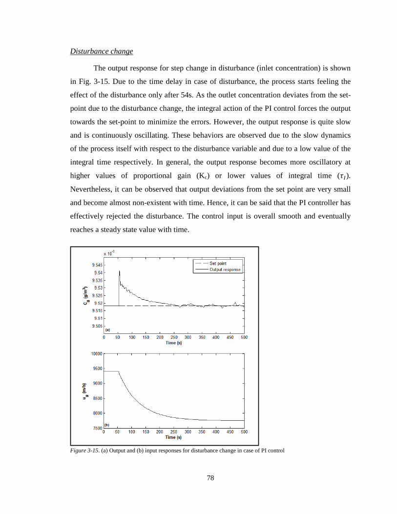
78
Disturbance change
The output response for step change in disturbance (inlet concentration) is shown
in Fig. 3-15. Due to the time delay in case of disturbance, the process starts feeling the
effect of the disturbance only after 54s. As the outlet concentration deviates from the set-
point due to the disturbance change, the integral action of the PI control forces the output
towards the set-point to minimize the errors. However, the output response is quite slow
and is continuously oscillating. These behaviors are observed due to the slow dynamics
of the process itself with respect to the disturbance variable and due to a low value of the
integral time respectively. In general, the output response becomes more oscillatory at
higher values of proportional gain (Kc) or lower values of integral time (𝜏𝐼).
Nevertheless, it can be observed that output deviations from the set point are very small
and become almost non-existent with time. Hence, it can be said that the PI controller has
effectively rejected the disturbance. The control input is overall smooth and eventually
reaches a steady state value with time.
Figure 3-15. (a) Output and (b) input responses for disturbance change in case of PI control

79
3.2.4.2 Analysis of FB-FF control system. The tuning parameters for the FB
controller are equal to parameter values listed in section 3.2.4.1 since adding a FF
controller has no effect on the performance of the PI controller. The transfer function for
the FF controller had already been determined in section 3.2.2.2.
Set-point change
The output response was the same as in Fig. 3-14 since the same PI controller was
used and the set-point change was made with no disturbance change. The behavior is
similar because the PI feedback controller deals with output deviations from the set-point
whereas the FF controller deals with the disturbance. Hence, when there are only set-
point changes (servo problem), the combined FB-FF corrective action has the entire
contribution from the PI controller.
Disturbance change
The output response for the step change in disturbance is shown in Fig. 3-16. It
can be clearly observed that the ideal FF controller has achieved almost perfect
disturbance rejection since the output is nearly close to the set-point throughout the
simulation time. Despite the oscillatory response, the controller performance is still
superior. The combined input response shows a smooth control action and is expected to
reach steady state condition eventually.
Overall, it had been observed that the FB-FF control system provided both good
set point tracking and nearly perfect disturbance rejection. Based on these responses, it
can be deduced that FB-FF control strategy offers superior performance when compared
with the conventional FB controller.
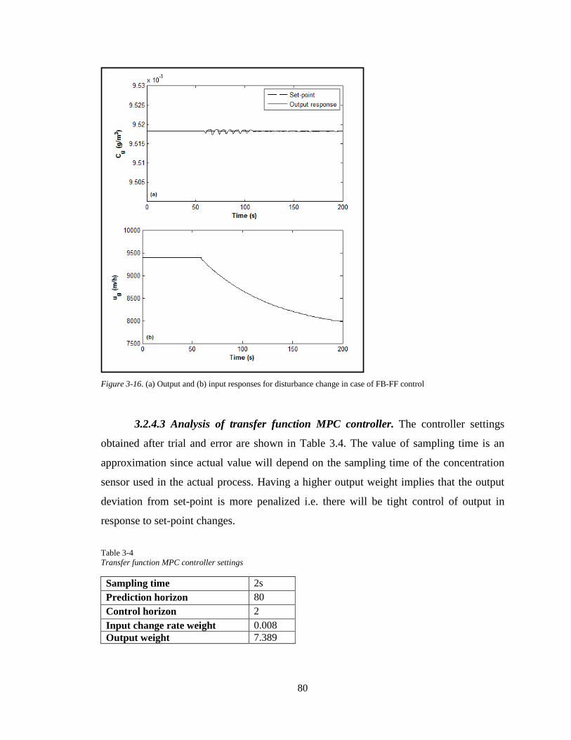
80
Figure 3-16. (a) Output and (b) input responses for disturbance change in case of FB-FF control
3.2.4.3 Analysis of transfer function MPC controller. The controller settings
obtained after trial and error are shown in Table 3.4. The value of sampling time is an
approximation since actual value will depend on the sampling time of the concentration
sensor used in the actual process. Having a higher output weight implies that the output
deviation from set-point is more penalized i.e. there will be tight control of output in
response to set-point changes.
Table 3-4 Transfer function MPC controller settings
Sampling time 2s Prediction horizon 80 Control horizon 2 Input change rate weight 0.008 Output weight 7.389
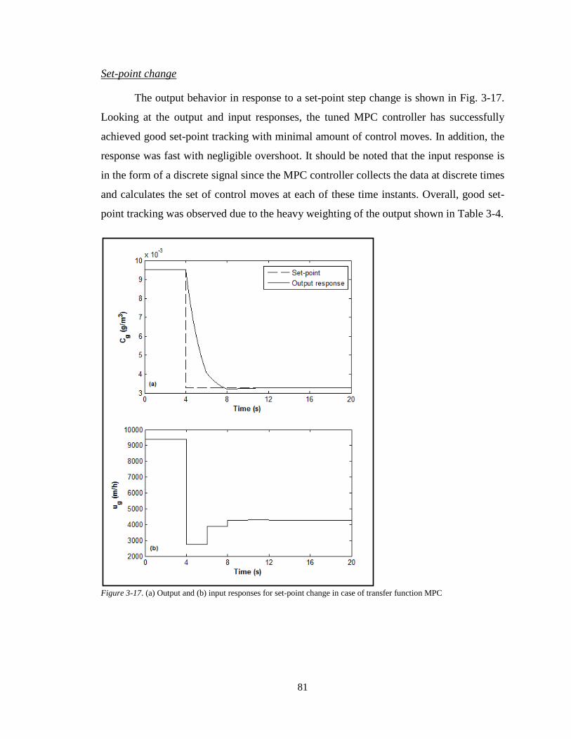
81
Set-point change
The output behavior in response to a set-point step change is shown in Fig. 3-17.
Looking at the output and input responses, the tuned MPC controller has successfully
achieved good set-point tracking with minimal amount of control moves. In addition, the
response was fast with negligible overshoot. It should be noted that the input response is
in the form of a discrete signal since the MPC controller collects the data at discrete times
and calculates the set of control moves at each of these time instants. Overall, good set-
point tracking was observed due to the heavy weighting of the output shown in Table 3-4.
Figure 3-17. (a) Output and (b) input responses for set-point change in case of transfer function MPC

82
Disturbance change
In case of step change in disturbance, the output response with MPC controller in
Fig. 3-18 is similar to the one with the FB controller in Fig. 3-15 except that the response
is smoother and less oscillatory. In response to the disturbance, a maximum output
deviation of 0.7% from the set-point is observed with the MPC controller. Although the
output response takes long time to reach the set-point value, the deviation errors are very
small. Hence, the MPC controller has successfully dealt with the disturbance effects.
Looking at the input response, the profile is continuous indicating excessive
implementation of control moves. This is because the deviation in the output response is
very small and to force the output back to the set-point very small changes in input are
required. Hence, the controller provides smooth and slow control action at the expense of
the control moves.
Figure 3-18. (a) Output and (b) input responses for disturbance change in case of transfer function MPC

83
3.2.4.4 Analysis of neural network MPC controller. The trained NN results and
the controller settings determined by trial-and-error are shown in Table 3-5. The MSE
and R2 values suggest that the NN model had been successfully trained. It can be seen
that the NNMPC controller requires a search parameter. This parameter is used for
controlling optimization performance of the controller [28].
Table 3-5 Trained NN and NNMPC controller setting results
NN Plant Identification results Total simulated data samples 1000
Sampling interval 2 s
Size of hidden layer 5
Validation MSE 2.81 x 10⁻⁸
Overall R2 value 0.998
Controller settings Maximum cost horizon (N2) 100
Control horizon 2
Control (input) weighting factor 1 x 10- 4
Search parameter 5 x 10⁻³
Set-point change
The output response for set-point change is shown in Fig. 3-19. It is observed that
the NNMPC controller provides excellent set-point tracking using less control moves.
However, there are time delays in the control actions of the controller. While training the
NN model in the NNMPC controller, the NNMPC control block in Simulink required
non-zero entry values for input and output delays so that the time variation of variables
could be accounted in the system. Hence, two delays on input and output were defined
for the NNMPC controller training that resulted in the response delays observed in
Fig. 3-19. Towards the end of the simulation time, it can be observed that there is a small
offset error between the new set-point value and the output response. Nevertheless, this
small discrepancy is eventually eliminated in the limit as time goes to infinity.
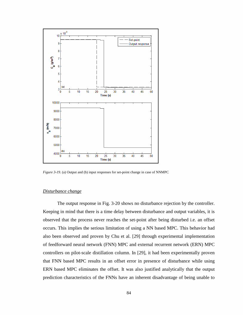
84
Figure 3-19. (a) Output and (b) input responses for set-point change in case of NNMPC
Disturbance change
The output response in Fig. 3-20 shows no disturbance rejection by the controller.
Keeping in mind that there is a time delay between disturbance and output variables, it is
observed that the process never reaches the set-point after being disturbed i.e. an offset
occurs. This implies the serious limitation of using a NN based MPC. This behavior had
also been observed and proven by Chu et al. [29] through experimental implementation
of feedforward neural network (FNN) MPC and external recurrent network (ERN) MPC
controllers on pilot-scale distillation column. In [29], it had been experimentally proven
that FNN based MPC results in an offset error in presence of disturbance while using
ERN based MPC eliminates the offset. It was also justified analytically that the output
prediction characteristics of the FNNs have an inherent disadvantage of being unable to

85
deal with model mismatch when the process is upset by a disturbance [29]. Based on the
justifications, Chu et al. claimed that using a FNN based MPC is unfeasible for practical
applications and that ERN based MPC should be used instead [29]. Since the NNMPC
controller in MATLAB uses a FNN model, it is clear that there will be an offset in case
of disturbance. Hence, based on the output responses observed towards set-point and
disturbance changes, it can be said that the NNMPC controller behaves like a
proportional only controller.
Figure 3-20. (a) Output and (b) input responses for disturbance change in case of NNMPC

86
3.2.4.5 Analysis of combined NNMPC and integral control. The design
properties of the controllers are shown in Table 3-6.
Table 3-6 NNMPC and integral controller properties
NNMPC Plant Identification results Total simulated data samples 1000
Sampling interval 2 s
Size of hidden layer 5
Validation MSE 3.48 x 10⁻¹⁰
Overall R2 value 0.999
Controller settings Maximum cost horizon (N2) 150
Control horizon 2
Control (input) weighting factor 1 x 10- 4
Search parameter 5 x 10⁻³
Integral gain (for integral controller) 8
Set-point change
The output response resulting from set-point change is shown in Fig. 3-21. It can
be seen that with the addition of an integral controller, the time delay that had been
observed for the NNMPC in Fig. 3-19 has been eliminated. Although, the combined
NNMPC-integral controller shows good set-point tracking, the output response has
overshoots. The overshoot occurs due to the combined control action of the two
controllers. In other words, the control signals from both the controllers add together,
resulting in a higher input value than the desired which causes the output to exceed the
set-point.

87
Figure 3-21. (a) Output and (b) input responses for set-point change in case of NNMPC-integral control
Disturbance change
It can be observed in Fig. 3-22 that the controller has managed to deal with
disturbance that had been initiated at the initial time. During the process upset (after the
time delay) by the disturbance, corrective action is initiated only by the integral controller
while the NNMPC becomes ineffective due to the reasons explained earlier in
section 3.2.4.4. Despite the disturbance rejection, there is a large overshoot where there is
141% deviation of the output from the desired set-point. The disadvantage of the additive
control action from the two controllers is the reason for the resulting overshoot. This
large overshoot is highly unacceptable in practical application since the outlet
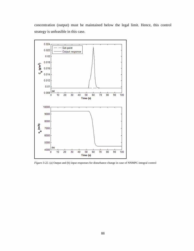
88
concentration (output) must be maintained below the legal limit. Hence, this control
strategy is unfeasible in this case.
Figure 3-22. (a) Output and (b) input responses for disturbance change in case of NNMPC-integral control

89
3.2.4.6 Comparison of BTF control strategies. Based on the analysis of the
control strategies in the previous sections, it can be deduced that three BTF control
strategies provided best control performance: 1) PI, 2) PI – FF, and 3) TF MPC based
control systems. To determine the optimum control strategy, these TF model based
control systems were qualitatively compared against each other for their performance
towards set-point and disturbance changes separately. The set-point changes consisted
of a set of random step changes ranging from 1.64 x 10⁻³ g/m3 (99% removal efficiency
with respect to base inlet concentration) to 9.518 x 10⁻³ g/m3 (base removal
efficiency of 94%). For analysis of disturbance rejection, a single disturbance step change
from base inlet concentration (0.164 g/m3) to a higher concentration (0.2 g/m3) at the
initial time was used. The results from all the controllers were compiled and plotted in the
same graph. The Simulink block diagram is provided in the Appendix.
Set-point changes
The output responses of the selected control strategies are shown in Fig. 3-23.
Overall, all the controllers showed excellent set-point tracking with TF MPC controller
showing the best control since there are no overshoots. In case of PI and PI-FF
controllers, there are overshoots which may be disadvantageous in situations where strict
control is needed. In case of a BTF process or any other environmental treatment
technology, this may be a serious consideration where safe pollutant release must be
below the legal limits. However, overshoots could be avoided by either decreasing
proportional gain or increasing the integral time at the expense of a sluggish response.
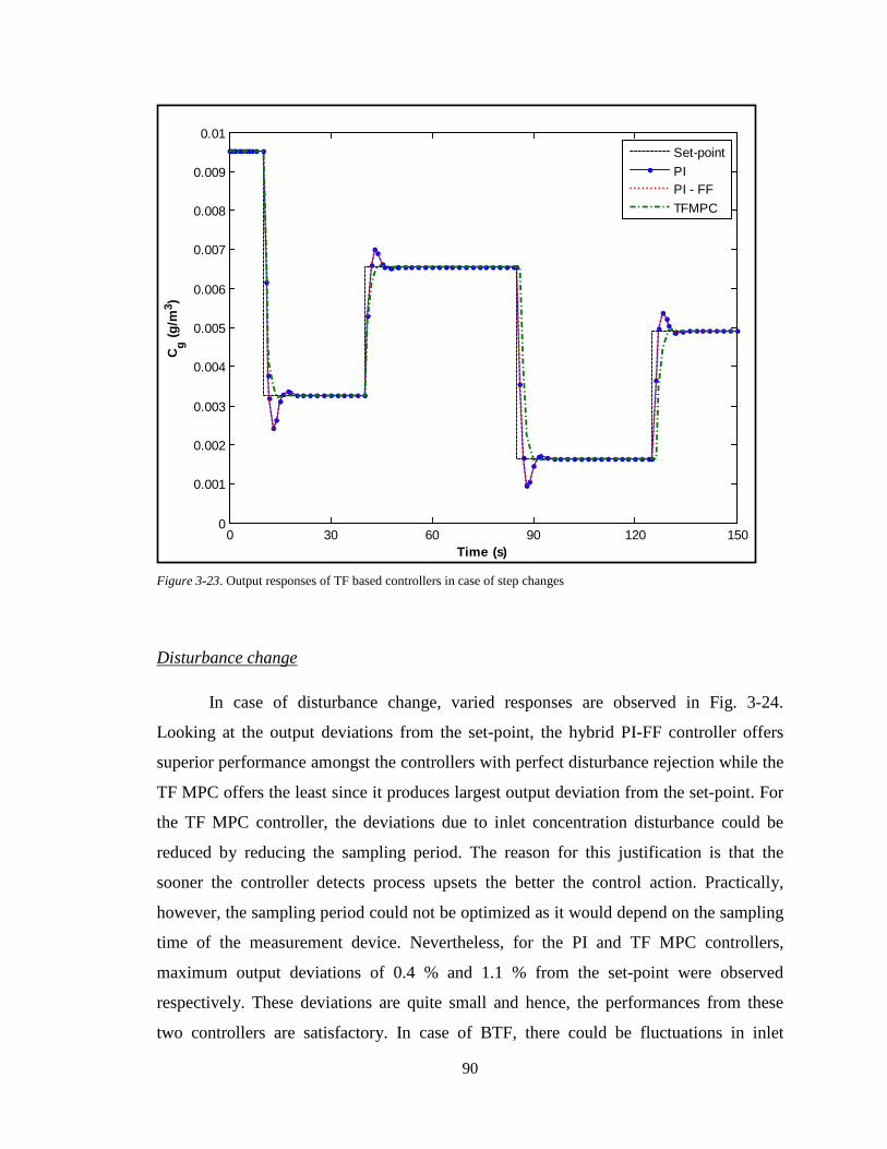
90
Figure 3-23. Output responses of TF based controllers in case of step changes
Disturbance change
In case of disturbance change, varied responses are observed in Fig. 3-24.
Looking at the output deviations from the set-point, the hybrid PI-FF controller offers
superior performance amongst the controllers with perfect disturbance rejection while the
TF MPC offers the least since it produces largest output deviation from the set-point. For
the TF MPC controller, the deviations due to inlet concentration disturbance could be
reduced by reducing the sampling period. The reason for this justification is that the
sooner the controller detects process upsets the better the control action. Practically,
however, the sampling period could not be optimized as it would depend on the sampling
time of the measurement device. Nevertheless, for the PI and TF MPC controllers,
maximum output deviations of 0.4 % and 1.1 % from the set-point were observed
respectively. These deviations are quite small and hence, the performances from these
two controllers are satisfactory. In case of BTF, there could be fluctuations in inlet
0 30 60 90 120 1500
0.001
0.002
0.003
0.004
0.005
0.006
0.007
0.008
0.009
0.01
Time (s)
C g (g/m
3 )
Set-pointPIPI - FFTFMPC
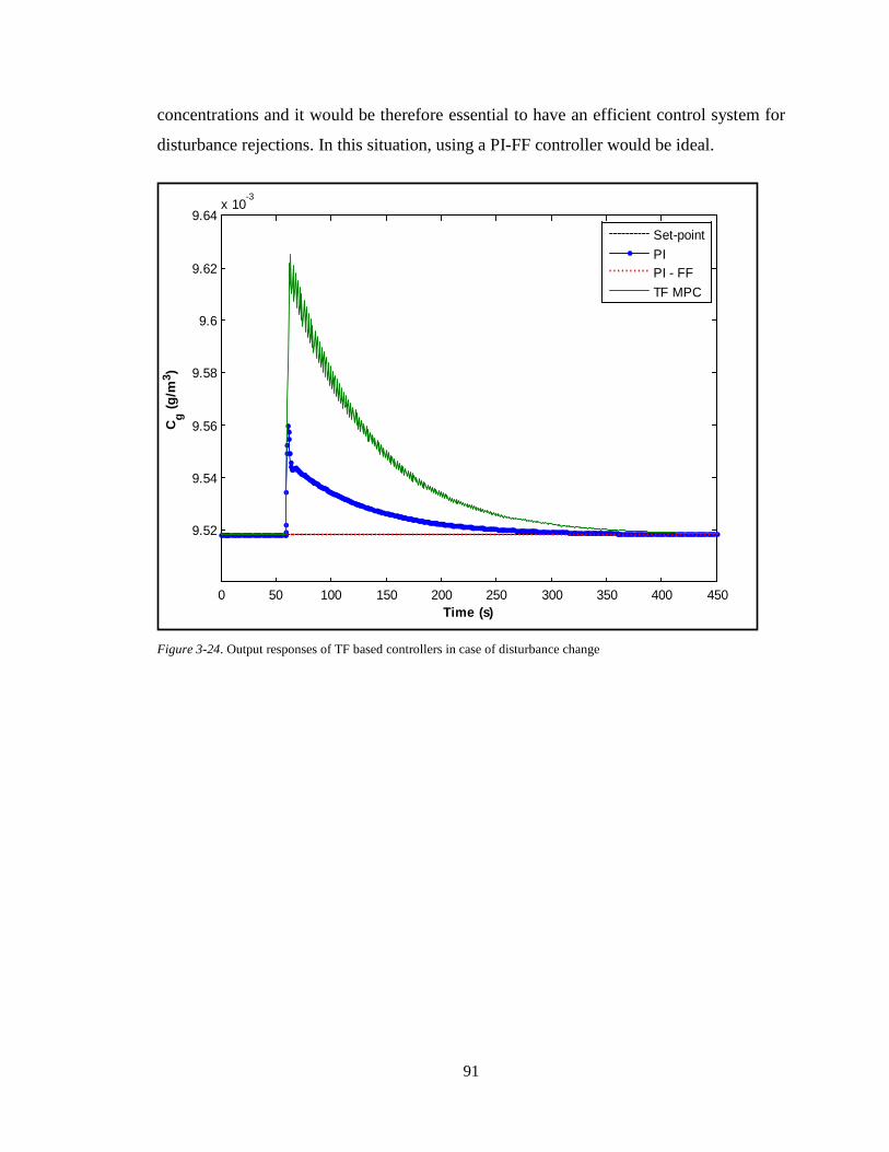
91
concentrations and it would be therefore essential to have an efficient control system for
disturbance rejections. In this situation, using a PI-FF controller would be ideal.
Figure 3-24. Output responses of TF based controllers in case of disturbance change
0 50 100 150 200 250 300 350 400 450
9.52
9.54
9.56
9.58
9.6
9.62
9.64x 10
-3
Time (s)
Cg (g
/m3 )
Set-pointPIPI - FFTF MPC

92
Chapter 4. Conclusion This work aimed to provide a theoretical aspect on the modeling and control of a
BTF for making it a viable air pollution treatment technology on a large-scale. The work
was focused on selecting an appropriate theoretical model from literature first that would
provide adequate insight into the dynamics and performance of a BTF in general. From
the review of five literature BTF models, it had been observed that the models were
mostly specific to the type of pollutants being treated. Although several achievements
were observed in these BTF models, there is still a need for an appropriate model that
could be universally used for practical applications. However, developing such model
may require a great deal of effort and time. Likewise, the theoretical analyses performed
in this work were based on a specific pollutant due to the specific nature of the selected
BTF model. Amongst the models reviewed, Kim and Deshusses’ model [5] was selected
as the target model with H2S being the target pollutant treated. The choice of the target
model selection was based on the simplicity of the mathematical model formulation while
at the same time capturing significant phenomena as well. Kim and Deshusses’ model [5]
had a simple model formulation which could be easily solved and also the model
captured many phenomena occurring in the BTF process. The most striking feature of the
model was its ability to simultaneously account for wetted and non-wetted biofilm due to
incomplete wetting of biofilm by the trickling liquid. However, the model was developed
for a differential BTF in batch mode and most of the model parameters were
experimental. For practical situations, a continuous operation of the BTF is required.
Moreover, there is also an issue on implementing and analyzing the performance of BTF
with the control strategies proposed in this work. Since the model parameters listed by
Kim and Deshusses [5] could not be used in case of a large continuous BTF, an
alternative strategy was used by considering cascaded n-batch BTFs in series. In this
configuration, the large BTF could be considered as a combination of differential BTFs
connected in series with each other. With the proposed configuration and some
modifications to the original model equations, the BTF reactor was scaled-up with
continuous mode of operation. Moreover, the need to determine new set of model
parameters for the large BTF was avoided. The original BTF model had been

93
successfully validated by Kim and Deshusses [5] with experimental data. Hence, it was
assumed that each of the differential BTFs in the proposed model structure behaved
exactly like the differential BTF in [5]. There could be an uncertainty in the reliability of
the proposed model to accurately represent the BTF dynamics in this case. Nevertheless,
the modified model was successfully simulated and analyzed for performance evaluation.
To solve the modified model where equations need to be solved for each reactor, a
pseudo steady state assumption was used. This strategy reduced the computational effort
and time required to solve the model. The performance was determined by analyzing the
effect of inlet concentration of H2S, gas velocity, and LGVR on the steady state outlet
concentration. The outlet concentration was directly related to inlet concentration and gas
velocity while a parabolic profile was observed in case of LGVR. This parabolic profile
indicated mass transfer effects occurring in the trickling liquid phase that affected the
removal efficiency of the pollutant. It had been observed that the inlet concentration and
gas velocity had strong affect on system performance while LGVR had effect only for a
small range.
For the implementation of control strategies on the BTF process, simple data
driven models were used. The modified model could not be used since it was still
computationally challenging in terms of effort and time. Moreover, controlling BTF
process based on the modified model would require continuous solution of the model
which is unfeasible. Hence, transfer function and neural network based models were
selected for identification of the BTF process. Assuming that the modified model
represents the actual BTF process, the TF and NN models were fitted with data from
simulation of the modified model. Gas velocity and inlet concentration were considered
as the main process inputs while outlet concentration was selected as the BTF
performance variable (output). The TF and NN models had been successfully obtained
with R2 values above 0.97 overall. For the NN model, the optimum size of the hidden
layer was 7 and the resulting NN model had a nearly perfect fit. However, the NN model
had been based on steady state data while the TF was fitted with dynamic step response
data. Hence, a TF model representation would be more accurate at this stage.
Finally, five control strategies were implemented namely PI, FB PI-FF, TF MPC,
NNMPC and NNMPC with integral control. The first three controllers were based on TF

94
model representation of BTF while the rest used NN model. For the control structure, gas
velocity, inlet concentration, and outlet concentration were selected as manipulated,
disturbance and controlled variables respectively. Through set-point and disturbance step
testing, it was found that the first three controllers provided satisfactory control
responses. While the NNMPC controller showed excellent set-point tracking, the
presence of a constant offset error in response to disturbance change was the main
limitation. The offset errors resulting from the use of NNMPC controller prove that using
FNN based model for MPC control is unfeasible and as suggested by [29], the use of
recurrent neural based models is recommended. Although the addition of an integral
controller to the NNMPC eliminated the offset error due to disturbance change, large
overshoots had been observed in response to set-point and disturbance changes. Since a
steady state NN model was used as the BTF plant model for the last two controllers
(NNMPC and NNMPC with integral controllers), it would be unjust to comment on the
performance of these controllers.
With regard to the theoretical model used for the BTF system, the modified Kim
and Deshusses’ model [5] could be more realistic by considering a change in biofilm
thickness due to biomass growth although it had been justified that H2S treating BTF
produce thin biofilms [5]. The effects of biomass growth can be easily implemented by
repeating the solution of the modified model with the pseudo steady state assumption at
different biofilm thickness. On the other hand, for practical implementation of the BTF
process, it would be essential to analyze the extent of BTF performance by considering
shock loading effects. For the BTF process, shock loading would refer to sudden large
change in the inlet concentration of the pollutant. It would be important to consider the
maximum shock loading as well to analyze the ability of the micro-organisms to
effectively remove the pollutant under extreme conditions and hence, investigate the
robustness of the BTF system. It is therefore recommended to consider shock loading
effects through experimental testing and model predictions. Finally, since the discussions
in this work are all based on theoretical analyses, it would be recommended to validate
the findings in this work with experimental testing.

95
References
[1] S. Mudlier et al., "Bioreactors for VOCs and odours - A review," Journal of Environmental Management, vol. 91, pp. 1039-1054, 2010.
[2] J. S. Devinny and J. Ramesh, "A phenomenological review of biofilter models," Chemical Engineering Journal, vol. 113, pp. 187-196, 2005.
[3] M. C. Delhomenie and M. Heitz, "Biofiltration of Air: A Review," Critical Reviews in Biotechnology, vol. 25, pp. 53-72, 2005.
[4] M. A. Deshusses and D. Gabriel, "Biotrickling Filter Technology," in Biotechnology for Odor and Air Pollution Control, Z. Shareefdeen and A. Singh, Eds., New York, Springer, 2005, pp. 147-166.
[5] S. Kim and M. A. Deshusses, "Development and Experimental Validation of a Conceptual Model for Biotrickling Filtration of H2S," Environmental Progress, vol. 22, no. 2, pp. 119-128, 2003.
[6] G. Soreanu et al., "Empirical modelling and dual-performance optimisation of a hydrogen sulphide removal process for biogas treatment," Bioresource Technology, vol. 101, pp. 9387-9390, 2010.
[7] E. R. Rene et al., "Back-propagation neural network for performance prediction in trickling bed air biofilter," International Journal of Environment and Pollution, vol. 28, no. 3-4, pp. 382-401, 2006. [Abstract].
[8] E. R. Rene et al., "Neural network models for biological waste-gas treatment systems," New Biotechnology, vol. 29, no. 1, pp. 56-73, December 2011.
[9] J. M. Yu et al., "Automatic control system for purifcation of H2S-contained waste gas with biotrickling filter," Journal of PLA University of Science and Technology (Natural Science Edition), vol. 9, no. 3, pp. 228-231, June 2008. [Abstract].
[10] C. Alonso et al., "Dynamic mathematical model for the Biodegradation of VOCs in a Biofilter: Biomass accumulation study," Environment Science & Technology, vol. 32, no. 20, pp. 3118-3123, 1998.
[11] Q. Liao et al., "Mathematical model for gas-liquid two-phase flow and biodegradation of a low concentration volatile organic (VOC) in a trickling biofilter," International Journal of Heat and Mass Transfer, vol. 51, pp. 1780-1792, 2008.

96
[12] S. Sharvelle et al., "Model Development for Biotrickling Filter Treatment of Graywater Simulant and Waste Gas. I," Journal of Environmental Engineering, vol. 134, no. 10, pp. 813-825, October 2008.
[13] S. Lee and A. J. Heber, "Ethylene removal using biotrickling filters: part II. Parameter estimation and mathematical simulation," Chemical Engineering Journal, vol. 158, pp. 89-99, 2010.
[14] B. I. Dvorak et al., "Evaluation of the Onda Correlations for Mass Transfer with Large Random Packings," Environmental Science & Technology, vol. 30, no. 3, pp. 945-953, 1996.
[15] J. R. Welty et al., Fundamentals of Momentum, Heat, and Mass Transfer, 5th ed., New Jersey: John Wiley & Sons, Inc., 2008.
[16] Matlab2R2009b2Help2Files, "ode23, ode45, ode113, ode15s, ode23s, ode23t, ode23tb," The Mathworks, Inc., 2009.
[17] MATLAB2R2009b2Help2Files, "fsolve," The Mathworks, Inc., 2009.
[18] D. E. Seborg et al., Process Dynamics and Control, 3rd ed., New Jersey: John Wiley & Sons, Inc., 2011.
[19] R. K. Pearson, "Nonlinear empirical modeling techniques," Computers and Chemical Engineering, vol. 30, p. 1514–1528, July 2006.
[20] W. L. Luyben, Process Modeling, Simulation, and Control for Chemical Engineers, 2nd ed., Boston: McGraw Hill, Inc., 1990.
[21] Loop-Pro TRAINER version 5.1, Tolland, Connecticut: Control Station, Inc., 2008.
[22] H. R. Maier and G. C. Dandy, "Neural Network Based Modelling of Environmental Variables: A Systematic Approach," Mathematical and Computer Modelling, vol. 33, pp. 669-682, 2001.
[23] H. Tang et al., Neural Networks: Computational Models and Applications, New York: Springer, 2007.
[24] O. J. Prado et al., "Retrofitting of an Industrial Chemical Scrubber into a Biotrickling Filter: Performance at a Gas Contact Time below 1 s," Journal of Environmental Engineering, vol. 135, no. 5, p. 359–366, May 2009.
[25] D. Gabriel et al., "Conversion of Full-Scale Wet Scrubbers to Biotrickling Filters for H2S Control at Publicly Owned Treatment Works," Journal of Environmental Engineering, vol. 130, no. 10, p. 1110–1117, October 2004.
97
[26] E. F. Camacho and C. Bordons, Model Predictive Control, London: Springer, 1999.
[27] Z. K. Nagy, "Model based control of a yeast fermentation bioreactor using optimally designed artificial neural networks," Chemical Engineering Journal, vol. 127, p. 95–109, 2007.
[28] B. ZareNezhad and A. Aminian, "Application of the Neural Network-Based Model Predictive Controllers In Nonlinear Industrial Systems. Case Study," Journal of the University of Chemical Technology and Metallurgy, vol. 46, no. 1, pp. 67-74, 2011.
[29] J. Chu et al., "Multistep Model Predictive Control Based on Artificial Neural Networks," Ind. Eng. Chem. Res., vol. 42, no. 21, pp. 5215-5228, 2003.

98
Appendix
MATLAB Codes for Biotrickling Filter Model Solutions
1. Kim & Deshusses’ [5] model solution
Function file for ODEs
function dC=gLbio_conc_profiles_lat(t,C,D,H,FT,N,kg,kL,r,A,Fg,FL,Vg,VL,Rm,Ks) a1=Fg/Vg; Aw=r*A; a2=(kg*Aw)/Vg; a3=(kg*Aw*((1-r)/r))/Vg; a4=FL/VL; a5=(kg*Aw)/VL; a6=(kL*Aw)/VL; a7=D/(FT^2); dCg(1)=-a2*(C(1)-H*C(N+1))-a3*(C(1)-H*C(12*N+1)); dCL(1)=a4*(C(2+N)-C(1+N))+a5*(C(1)-H*C(1+N))-a6*(C(1+N)-C(1+2*N)); for j=2:N-1 dCg(j)=a1*(C(j-1)-C(j))-a2*(C(j)-H*C(j+N))-a3*(C(j)-H*C(j+12*N)); dCL(j)=a4*(C(j+1+N)-C(j+N))+a5*(C(j)-H*C(j+N))-a6*(C(j+N)-C(j+2*N)); end dCg(N)=a1*(C(N-1)-C(N))-a2*(C(N)-H*C(N+N))-a3*(C(N)-H*C(N+12*N)); dCL(N)=a5*(C(N)-H*C(N+N))-a6*(C(N+N)-C(N+2*N)); for j=1:N dCwb_interface(j)=a7*(C(j+N)-2*C(j+2*N)+C(j+3*N))-((Rm*C(j+2*N))/(Ks+C(j+2*N))); dCnwb_interface(j)=a7*((C(j)/H)-2*C(j+12*N)+C(j+13*N))-((Rm*C(j+12*N))/(Ks+C(j+12*N))); dCwb_iN(j)=a7*(C(j+10*N)-C(j+11*N))-((Rm*C(j+11*N))/(Ks+C(j+11*N))); dCnwb_iN(j)=a7*(C(j+20*N)-C(j+21*N))-((Rm*C(j+21*N))/(Ks+C(j+21*N))); end for j=1:N dCwbi2(j)=a7*(C(2*N+j)-2*C((2+1)*N+j)+C((2+2)*N+j))-((Rm*C((2+1)*N+j))/(Ks+C((2+1)*N+j))); dCwbi3(j)=a7*(C(3*N+j)-2*C((3+1)*N+j)+C((3+2)*N+j))-((Rm*C((3+1)*N+j))/(Ks+C((3+1)*N+j))); dCwbi4(j)=a7*(C(4*N+j)-2*C((4+1)*N+j)+C((4+2)*N+j))-((Rm*C((4+1)*N+j))/(Ks+C((4+1)*N+j))); dCwbi5(j)=a7*(C(5*N+j)-2*C((5+1)*N+j)+C((5+2)*N+j))-((Rm*C((5+1)*N+j))/(Ks+C((5+1)*N+j))); dCwbi6(j)=a7*(C(6*N+j)-2*C((6+1)*N+j)+C((6+2)*N+j))-((Rm*C((6+1)*N+j))/(Ks+C((6+1)*N+j))); dCwbi7(j)=a7*(C(7*N+j)-2*C((7+1)*N+j)+C((7+2)*N+j))-((Rm*C((7+1)*N+j))/(Ks+C((7+1)*N+j)));

99
dCwbi8(j)=a7*(C(8*N+j)-2*C((8+1)*N+j)+C((8+2)*N+j))-((Rm*C((8+1)*N+j))/(Ks+C((8+1)*N+j))); dCwbi9(j)=a7*(C(9*N+j)-2*C((9+1)*N+j)+C((9+2)*N+j))-((Rm*C((9+1)*N+j))/(Ks+C((9+1)*N+j))); dCnwbi2(j)=a7*(C((2+10)*N+j)-2*C((2+1+10)*N+j)+C((2+2+10)*N+j))-((Rm*C((2+1+10)*N+j))/(Ks+C((2+1+10)*N+j))); dCnwbi3(j)=a7*(C((3+10)*N+j)-2*C((3+1+10)*N+j)+C((3+2+10)*N+j))-((Rm*C((3+1+10)*N+j))/(Ks+C((3+1+10)*N+j))); dCnwbi4(j)=a7*(C((4+10)*N+j)-2*C((4+1+10)*N+j)+C((4+2+10)*N+j))-((Rm*C((4+1+10)*N+j))/(Ks+C((4+1+10)*N+j))); dCnwbi5(j)=a7*(C((5+10)*N+j)-2*C((5+1+10)*N+j)+C((5+2+10)*N+j))-((Rm*C((5+1+10)*N+j))/(Ks+C((5+1+10)*N+j))); dCnwbi6(j)=a7*(C((6+10)*N+j)-2*C((6+1+10)*N+j)+C((6+2+10)*N+j))-((Rm*C((6+1+10)*N+j))/(Ks+C((6+1+10)*N+j))); dCnwbi7(j)=a7*(C((7+10)*N+j)-2*C((7+1+10)*N+j)+C((7+2+10)*N+j))-((Rm*C((7+1+10)*N+j))/(Ks+C((7+1+10)*N+j))); dCnwbi8(j)=a7*(C((8+10)*N+j)-2*C((8+1+10)*N+j)+C((8+2+10)*N+j))-((Rm*C((8+1+10)*N+j))/(Ks+C((8+1+10)*N+j))); dCnwbi9(j)=a7*(C((9+10)*N+j)-2*C((9+1+10)*N+j)+C((9+2+10)*N+j))-((Rm*C((9+1+10)*N+j))/(Ks+C((9+1+10)*N+j))); end dC=[dCg'; dCL'; dCwb_interface'; dCwbi2'; dCwbi3'; dCwbi4'; dCwbi5'; dCwbi6'; dCwbi7'; dCwbi8'; dCwbi9'; dCwb_iN'; dCnwb_interface'; dCnwbi2'; dCnwbi3'; dCnwbi4'; dCnwbi5'; dCnwbi6'; dCnwbi7'; dCnwbi8'; dCnwbi9'; dCnwb_iN']; M-file for solution
% Kim & Deshusses' Original Model Simulation (2003) uL=11.8; % Trickling rate (m3/m2.h) ug=9400; % Gas flow rate (m3/m2.h) N=10; % No of segments along the height of BTF/biofilm FT=(23e-6)/N; % Biofilm thickness (m) Rm=58400; % Max reaction rate (g.m3/h) Ks=0.0279; % Michaelis-Menten constant (g/m3)

100
H=0.387; % Henry's constant D=5.796e-6; % H2S Diffusion coefficient (m2/h) Dg=0.016332; % H2S diffusion in gas using Fuller correlation at 25C and 1 atm (m2/h) a=600; % Specific interfacial area (m2/m3) Dp=0.04; % Size of packing (m) rhoL=1007; % Density of water (trickling liquid) (kg/m3) rhog=1.1845; % Density of gas (kg/m3) mL=3600*0.0008904; % Viscosity of water at 25C (kg/m.h) mg=0.0678; % Viscosity of gas from HYSYS (kg/m.h) gc=1.271376e8; % Acc. due to gravity (m/h2) stw=933120; % Surface tension of water at room temperature (kg/h2) ab=Dp^2; % Cross-sectional area of bed (m2) FL=uL*ab; % Volumetric flow rate of liquid (m3/h) Fg=ug*ab; % Volumetric flow rate of gas (m3/h) L=uL*rhoL; % Superficial liq. mass velocity(kg/m2.h) G=ug*rhog; % Superficial gas mass velocity (kg/m2.h) V=Dp^3; % Volume of bed (m3) A=a*V; % Interfacial Area (m2) % Finding surface tension term in equation 13 rr=0.2298; % Wetting ratio at FL=0.01888 m3/h uLL=11.8; % Trickling rate (m3/m2.h) FLL=uLL*ab; % Volumetric flow rate of liquid (m3/h) LL=uLL*rhoL; % Superficial liq. mass velocity (kg/m2.h) Ree=LL/a/mL; % Reynolds number Frr=(a*LL^2)/gc/(rhoL^2); % Froude number Wee=(LL^2)/rhoL/stw/a; % Weber number STR=-log(1-rr)/(1.45*(Ree^0.1)*(Frr^(-0.05))*(Wee^0.2)); % Surface tension ratio term in equation 13 % Finding wetting ratio, wetted area and specific wetted area Re=L/a/mL; % Reynolds number Fr=(a*L^2)/gc/(rhoL^2); % Froude number We=(L^2)/rhoL/stw/a; % Weber number r=1-exp(-1.45*STR*(Re^0.1)*(Fr^(-0.05))*(We^0.2)); % Wetting ratio Aw=r*A; % Wetted area (m2) aw=Aw/V; % Specific wetted area (m2/m3) % Finding mass transfer coefficients kg=5.23*((G/(a*mg))^0.7)*((mg/(rhog*Dg))^(1/3))*((a*Dp)^(-2))*a*Dg; % Gas-Liq mass transfer coefficient (m/h) kL=0.0051*((L/(aw*mL))^(2/3))*((mL/(rhoL*D))^(-0.5))*((a*Dp)^0.4)*((rhoL/(mL*gc))^(-1/3)); % Liq-biofilm mass transfer coefficient (m/h) % Finding Gas and Liquid Volumes VL=(0.00001*FL)+0.0000008; % Dynamic holdup/liq. phase volume (m3)

101
Vol_ratio=8.6e4; % Gas/liquid Volume ratio Vg=Vol_ratio*VL; % Gas phase volume (m3) % Solution tspan=[0 2]; Cg0=0.164; % Initial concentration of H2S (g/m3) C0=zeros(22*N,1); C0(1,1)=Cg0; C0(N+1,1)=Cg0/H; C0(12*N+1,1)=Cg0/H; [t,C]=ode23s(@gLbio_conc_profiles_lat,tspan,C0,[],D,H,FT,N,kg,kL,r,A,Fg,FL,Vg,VL,Rm,Ks) Time1=[0 0.0132 0.046 0.0658 0.0921 0.112 0.138 0.164 0.1908 0.2171 0.25 0.283 0.322 0.349 0.388 0.428 0.474 0.513 0.566 0.632 0.704 0.803 0.941 1.059 1.257 1.368 1.533 1.717 1.967]; High_Conc_Exp=[0.1640 0.1633 0.1577 0.1542 0.15 0.1451 0.1408 0.1352 0.131 0.1261 0.1218 0.1169 0.112 0.1077 0.1035 0.0986 0.0944 0.0894 0.0845 0.0782 0.0725 0.0655 0.0549 0.0465 0.0345 0.0289 0.0225 0.0162 0.00986]; plot(t,C(:,1),Time1,High_Conc_Exp,'*') hold on % ------------- Low Inlet Concentration ------------------------------ Cg0=0.08592; % Initial concentration of H2S (g/m3) C0=zeros(22*N,1); C0(1,1)=Cg0; C0(N+1,1)=Cg0/H; C0(12*N+1,1)=Cg0/H; kL=0.0051*((L/(aw*mL))^(2/3))*((mL/(rhoL*D))^(-0.5))*((a*Dp)^0.4)*((rhoL/(mL*gc))^(-1/3)); % Liq-biofilm mass transfer coefficient (m/h) [tlow,C_low]=ode23s(@gLbio_conc_profiles_lat,tspan,C0,[],D,H,FT,N,kg,kL,r,A,Fg,FL,Vg,VL,Rm,Ks) Time2=[0 0.0395 0.0658 0.0789 0.1053 0.125 0.1579 0.1908 0.2171 0.2434 0.2763 0.3158 0.3421 0.3816 0.4211 0.4605 0.5132 0.5632 0.625 0.6974 0.7895 0.9342 1.0526]; Low_Conc_Exp=[0.08592 0.07958 0.07465 0.07183 0.06761 0.06408 0.05986 0.05634 0.05211 0.04930 0.04577 0.04225 0.03803 0.03521 0.03239 0.02958 0.02535 0.02254 0.01972 0.01620 0.01268 0.00845 0.00423]; plot(tlow,C_low(:,1),'-.',Time2,Low_Conc_Exp,'o') xlabel('\bfTime (h)') ylabel('\bfInlet H_2S Concentration (g/m^3)') legend('Model High Conc.','Exp. Data High Conc.','Model Low Conc.','Exp. Data Low Conc.') axis([-inf inf 0 0.18]) hold off
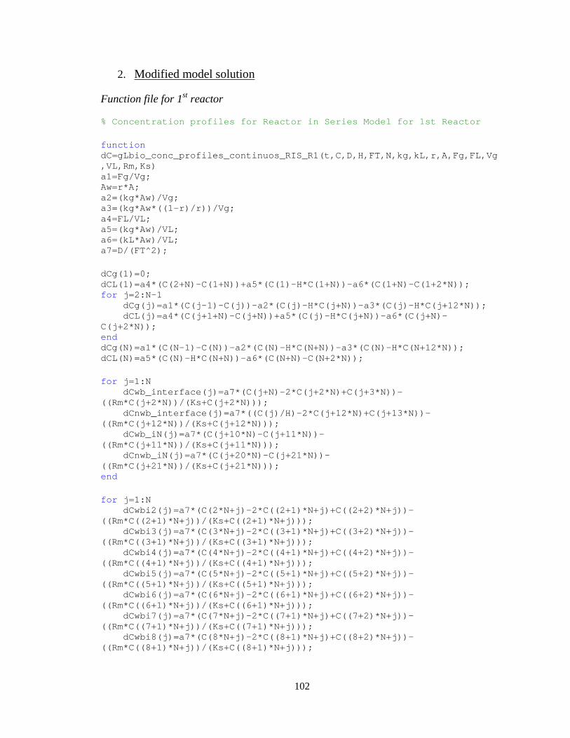
102
2. Modified model solution
Function file for 1st reactor
% Concentration profiles for Reactor in Series Model for 1st Reactor function dC=gLbio_conc_profiles_continuos_RIS_R1(t,C,D,H,FT,N,kg,kL,r,A,Fg,FL,Vg,VL,Rm,Ks) a1=Fg/Vg; Aw=r*A; a2=(kg*Aw)/Vg; a3=(kg*Aw*((1-r)/r))/Vg; a4=FL/VL; a5=(kg*Aw)/VL; a6=(kL*Aw)/VL; a7=D/(FT^2); dCg(1)=0; dCL(1)=a4*(C(2+N)-C(1+N))+a5*(C(1)-H*C(1+N))-a6*(C(1+N)-C(1+2*N)); for j=2:N-1 dCg(j)=a1*(C(j-1)-C(j))-a2*(C(j)-H*C(j+N))-a3*(C(j)-H*C(j+12*N)); dCL(j)=a4*(C(j+1+N)-C(j+N))+a5*(C(j)-H*C(j+N))-a6*(C(j+N)-C(j+2*N)); end dCg(N)=a1*(C(N-1)-C(N))-a2*(C(N)-H*C(N+N))-a3*(C(N)-H*C(N+12*N)); dCL(N)=a5*(C(N)-H*C(N+N))-a6*(C(N+N)-C(N+2*N)); for j=1:N dCwb_interface(j)=a7*(C(j+N)-2*C(j+2*N)+C(j+3*N))-((Rm*C(j+2*N))/(Ks+C(j+2*N))); dCnwb_interface(j)=a7*((C(j)/H)-2*C(j+12*N)+C(j+13*N))-((Rm*C(j+12*N))/(Ks+C(j+12*N))); dCwb_iN(j)=a7*(C(j+10*N)-C(j+11*N))-((Rm*C(j+11*N))/(Ks+C(j+11*N))); dCnwb_iN(j)=a7*(C(j+20*N)-C(j+21*N))-((Rm*C(j+21*N))/(Ks+C(j+21*N))); end for j=1:N dCwbi2(j)=a7*(C(2*N+j)-2*C((2+1)*N+j)+C((2+2)*N+j))-((Rm*C((2+1)*N+j))/(Ks+C((2+1)*N+j))); dCwbi3(j)=a7*(C(3*N+j)-2*C((3+1)*N+j)+C((3+2)*N+j))-((Rm*C((3+1)*N+j))/(Ks+C((3+1)*N+j))); dCwbi4(j)=a7*(C(4*N+j)-2*C((4+1)*N+j)+C((4+2)*N+j))-((Rm*C((4+1)*N+j))/(Ks+C((4+1)*N+j))); dCwbi5(j)=a7*(C(5*N+j)-2*C((5+1)*N+j)+C((5+2)*N+j))-((Rm*C((5+1)*N+j))/(Ks+C((5+1)*N+j))); dCwbi6(j)=a7*(C(6*N+j)-2*C((6+1)*N+j)+C((6+2)*N+j))-((Rm*C((6+1)*N+j))/(Ks+C((6+1)*N+j))); dCwbi7(j)=a7*(C(7*N+j)-2*C((7+1)*N+j)+C((7+2)*N+j))-((Rm*C((7+1)*N+j))/(Ks+C((7+1)*N+j))); dCwbi8(j)=a7*(C(8*N+j)-2*C((8+1)*N+j)+C((8+2)*N+j))-((Rm*C((8+1)*N+j))/(Ks+C((8+1)*N+j)));

103
dCwbi9(j)=a7*(C(9*N+j)-2*C((9+1)*N+j)+C((9+2)*N+j))-((Rm*C((9+1)*N+j))/(Ks+C((9+1)*N+j))); dCnwbi2(j)=a7*(C((2+10)*N+j)-2*C((2+1+10)*N+j)+C((2+2+10)*N+j))-((Rm*C((2+1+10)*N+j))/(Ks+C((2+1+10)*N+j))); dCnwbi3(j)=a7*(C((3+10)*N+j)-2*C((3+1+10)*N+j)+C((3+2+10)*N+j))-((Rm*C((3+1+10)*N+j))/(Ks+C((3+1+10)*N+j))); dCnwbi4(j)=a7*(C((4+10)*N+j)-2*C((4+1+10)*N+j)+C((4+2+10)*N+j))-((Rm*C((4+1+10)*N+j))/(Ks+C((4+1+10)*N+j))); dCnwbi5(j)=a7*(C((5+10)*N+j)-2*C((5+1+10)*N+j)+C((5+2+10)*N+j))-((Rm*C((5+1+10)*N+j))/(Ks+C((5+1+10)*N+j))); dCnwbi6(j)=a7*(C((6+10)*N+j)-2*C((6+1+10)*N+j)+C((6+2+10)*N+j))-((Rm*C((6+1+10)*N+j))/(Ks+C((6+1+10)*N+j))); dCnwbi7(j)=a7*(C((7+10)*N+j)-2*C((7+1+10)*N+j)+C((7+2+10)*N+j))-((Rm*C((7+1+10)*N+j))/(Ks+C((7+1+10)*N+j))); dCnwbi8(j)=a7*(C((8+10)*N+j)-2*C((8+1+10)*N+j)+C((8+2+10)*N+j))-((Rm*C((8+1+10)*N+j))/(Ks+C((8+1+10)*N+j))); dCnwbi9(j)=a7*(C((9+10)*N+j)-2*C((9+1+10)*N+j)+C((9+2+10)*N+j))-((Rm*C((9+1+10)*N+j))/(Ks+C((9+1+10)*N+j))); end dCnwb_interface(1)=0; dC=[dCg'; dCL'; dCwb_interface'; dCwbi2'; dCwbi3'; dCwbi4'; dCwbi5'; dCwbi6'; dCwbi7'; dCwbi8'; dCwbi9'; dCwb_iN'; dCnwb_interface'; dCnwbi2'; dCnwbi3'; dCnwbi4'; dCnwbi5'; dCnwbi6'; dCnwbi7'; dCnwbi8'; dCnwbi9'; dCnwb_iN'];
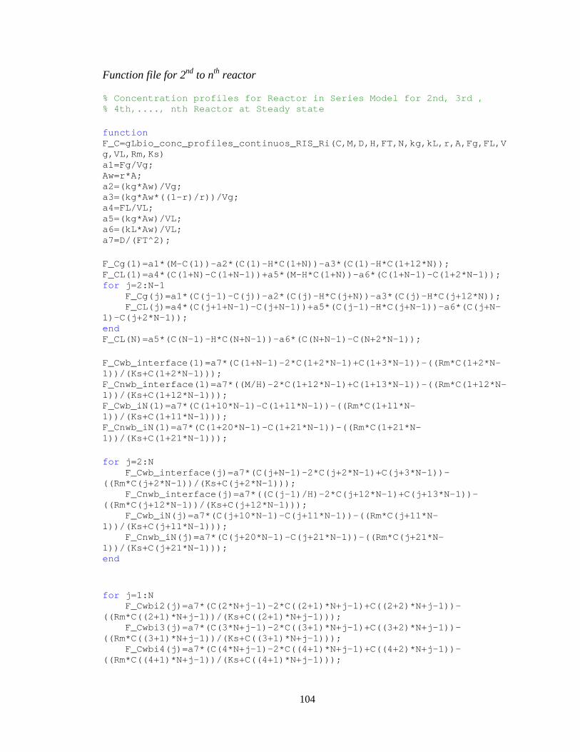
104
Function file for 2nd to nth reactor
% Concentration profiles for Reactor in Series Model for 2nd, 3rd , % 4th,...., nth Reactor at Steady state function F_C=gLbio_conc_profiles_continuos_RIS_Ri(C,M,D,H,FT,N,kg,kL,r,A,Fg,FL,Vg,VL,Rm,Ks) a1=Fg/Vg; Aw=r*A; a2=(kg*Aw)/Vg; a3=(kg*Aw*((1-r)/r))/Vg; a4=FL/VL; a5=(kg*Aw)/VL; a6=(kL*Aw)/VL; a7=D/(FT^2); F_Cg(1)=a1*(M-C(1))-a2*(C(1)-H*C(1+N))-a3*(C(1)-H*C(1+12*N)); F_CL(1)=a4*(C(1+N)-C(1+N-1))+a5*(M-H*C(1+N))-a6*(C(1+N-1)-C(1+2*N-1)); for j=2:N-1 F_Cg(j)=a1*(C(j-1)-C(j))-a2*(C(j)-H*C(j+N))-a3*(C(j)-H*C(j+12*N)); F_CL(j)=a4*(C(j+1+N-1)-C(j+N-1))+a5*(C(j-1)-H*C(j+N-1))-a6*(C(j+N-1)-C(j+2*N-1)); end F_CL(N)=a5*(C(N-1)-H*C(N+N-1))-a6*(C(N+N-1)-C(N+2*N-1)); F_Cwb_interface(1)=a7*(C(1+N-1)-2*C(1+2*N-1)+C(1+3*N-1))-((Rm*C(1+2*N-1))/(Ks+C(1+2*N-1))); F_Cnwb_interface(1)=a7*((M/H)-2*C(1+12*N-1)+C(1+13*N-1))-((Rm*C(1+12*N-1))/(Ks+C(1+12*N-1))); F_Cwb_iN(1)=a7*(C(1+10*N-1)-C(1+11*N-1))-((Rm*C(1+11*N-1))/(Ks+C(1+11*N-1))); F_Cnwb_iN(1)=a7*(C(1+20*N-1)-C(1+21*N-1))-((Rm*C(1+21*N-1))/(Ks+C(1+21*N-1))); for j=2:N F_Cwb_interface(j)=a7*(C(j+N-1)-2*C(j+2*N-1)+C(j+3*N-1))-((Rm*C(j+2*N-1))/(Ks+C(j+2*N-1))); F_Cnwb_interface(j)=a7*((C(j-1)/H)-2*C(j+12*N-1)+C(j+13*N-1))-((Rm*C(j+12*N-1))/(Ks+C(j+12*N-1))); F_Cwb_iN(j)=a7*(C(j+10*N-1)-C(j+11*N-1))-((Rm*C(j+11*N-1))/(Ks+C(j+11*N-1))); F_Cnwb_iN(j)=a7*(C(j+20*N-1)-C(j+21*N-1))-((Rm*C(j+21*N-1))/(Ks+C(j+21*N-1))); end for j=1:N F_Cwbi2(j)=a7*(C(2*N+j-1)-2*C((2+1)*N+j-1)+C((2+2)*N+j-1))-((Rm*C((2+1)*N+j-1))/(Ks+C((2+1)*N+j-1))); F_Cwbi3(j)=a7*(C(3*N+j-1)-2*C((3+1)*N+j-1)+C((3+2)*N+j-1))-((Rm*C((3+1)*N+j-1))/(Ks+C((3+1)*N+j-1))); F_Cwbi4(j)=a7*(C(4*N+j-1)-2*C((4+1)*N+j-1)+C((4+2)*N+j-1))-((Rm*C((4+1)*N+j-1))/(Ks+C((4+1)*N+j-1)));

105
F_Cwbi5(j)=a7*(C(5*N+j-1)-2*C((5+1)*N+j-1)+C((5+2)*N+j-1))-((Rm*C((5+1)*N+j-1))/(Ks+C((5+1)*N+j-1))); F_Cwbi6(j)=a7*(C(6*N+j-1)-2*C((6+1)*N+j-1)+C((6+2)*N+j-1))-((Rm*C((6+1)*N+j-1))/(Ks+C((6+1)*N+j-1))); F_Cwbi7(j)=a7*(C(7*N+j-1)-2*C((7+1)*N+j-1)+C((7+2)*N+j-1))-((Rm*C((7+1)*N+j-1))/(Ks+C((7+1)*N+j-1))); F_Cwbi8(j)=a7*(C(8*N+j-1)-2*C((8+1)*N+j-1)+C((8+2)*N+j-1))-((Rm*C((8+1)*N+j-1))/(Ks+C((8+1)*N+j-1))); F_Cwbi9(j)=a7*(C(9*N+j-1)-2*C((9+1)*N+j-1)+C((9+2)*N+j-1))-((Rm*C((9+1)*N+j-1))/(Ks+C((9+1)*N+j-1))); F_Cnwbi2(j)=a7*(C((2+10)*N+j-1)-2*C((2+1+10)*N+j-1)+C((2+2+10)*N+j-1))-((Rm*C((2+1+10)*N+j-1))/(Ks+C((2+1+10)*N+j-1))); F_Cnwbi3(j)=a7*(C((3+10)*N+j-1)-2*C((3+1+10)*N+j-1)+C((3+2+10)*N+j-1))-((Rm*C((3+1+10)*N+j-1))/(Ks+C((3+1+10)*N+j-1))); F_Cnwbi4(j)=a7*(C((4+10)*N+j-1)-2*C((4+1+10)*N+j-1)+C((4+2+10)*N+j-1))-((Rm*C((4+1+10)*N+j-1))/(Ks+C((4+1+10)*N+j-1))); F_Cnwbi5(j)=a7*(C((5+10)*N+j-1)-2*C((5+1+10)*N+j-1)+C((5+2+10)*N+j-1))-((Rm*C((5+1+10)*N+j-1))/(Ks+C((5+1+10)*N+j-1))); F_Cnwbi6(j)=a7*(C((6+10)*N+j-1)-2*C((6+1+10)*N+j-1)+C((6+2+10)*N+j-1))-((Rm*C((6+1+10)*N+j-1))/(Ks+C((6+1+10)*N+j-1))); F_Cnwbi7(j)=a7*(C((7+10)*N+j-1)-2*C((7+1+10)*N+j-1)+C((7+2+10)*N+j-1))-((Rm*C((7+1+10)*N+j-1))/(Ks+C((7+1+10)*N+j-1))); F_Cnwbi8(j)=a7*(C((8+10)*N+j-1)-2*C((8+1+10)*N+j-1)+C((8+2+10)*N+j-1))-((Rm*C((8+1+10)*N+j-1))/(Ks+C((8+1+10)*N+j-1))); F_Cnwbi9(j)=a7*(C((9+10)*N+j-1)-2*C((9+1+10)*N+j-1)+C((9+2+10)*N+j-1))-((Rm*C((9+1+10)*N+j-1))/(Ks+C((9+1+10)*N+j-1))); end F_C=[F_Cg'; F_CL'; F_Cwb_interface'; F_Cwbi2'; F_Cwbi3'; F_Cwbi4'; F_Cwbi5'; F_Cwbi6'; F_Cwbi7'; F_Cwbi8'; F_Cwbi9'; F_Cwb_iN'; F_Cnwb_interface'; F_Cnwbi2'; F_Cnwbi3'; F_Cnwbi4'; F_Cnwbi5'; F_Cnwbi6'; F_Cnwbi7'; F_Cnwbi8'; F_Cnwbi9'; F_Cnwb_iN'];

106
M-file for solution
% Kim & Deshusses Modified Model (2003) % CONTINUOS MODE OF OPERATION for Reactor in Series Model uL=11.8; % Trickling rate (m3/m2.h) ug=9400; % Gas flow rate (m3/m2.h) N=10; % No of segments along the height of BTF/biofilm FT=(23e-6)/N; % Biofilm thickness (m) Rm=58400; % Max reaction rate (g.m3/h) Ks=0.0279; % Michaelis-Menten constant (g/m3) H=0.387; % Henry's constant D=5.796e-6; % H2S Diffusion coefficient (m2/h) Dg=0.016332; % H2S diffusion in gas using Fuller correlation at 25C and 1 atm (m2/h) a=600; % Specific interfacial area (m2/m3) Dp=0.04; % Size of packing (m) rhoL=1007; % Density of water (trickling liquid) (kg/m3) rhog=1.1845; % Density of gas (kg/m3) mL=3600*0.0008904; % Viscosity of water at 25C (kg/m.h) mg=0.0678; % Viscosity of gas from HYSYS (kg/m.h) gc=1.271376e8; % Acc. due to gravity (m/h2) stw=933120; % Surface tension of water at room temperature (kg/h2) ab=Dp^2; % Cross-sectional area of bed (m2) FL=uL*ab; % Volumetric flow rate of liquid (m3/h) Fg=ug*ab; % Volumetric flow rate of gas (m3/h) L=uL*rhoL; % Superficial liq. mass velocity (kg/m2.h) G=ug*rhog; % Superficial gas mass velocity (kg/m2.h) V=Dp^3; % Volume of bed (m3) A=a*V; % Interfacial Area (m2) % Finding surface tension term in equation 13 rr=0.2298; % Wetting ratio at FL=0.01888 m3/h uLL=11.8; % Trickling rate (m3/m2.h) FLL=uLL*ab; % Volumetric flow rate of liquid (m3/h) LL=uLL*rhoL; % Superficial liq. mass velocity (kg/m2.h) Ree=LL/a/mL; % Reynolds number Frr=(a*LL^2)/gc/(rhoL^2); % Froude number Wee=(LL^2)/rhoL/stw/a; % Weber number STR=-log(1-rr)/(1.45*(Ree^0.1)*(Frr^(-0.05))*(Wee^0.2)); % Surface tension ratio term in equation 13 % Finding wetting ratio, wetted area and specific wetted area Re=L/a/mL; % Reynolds number Fr=(a*L^2)/gc/(rhoL^2); % Froude number We=(L^2)/rhoL/stw/a; % Weber number r=1-exp(-1.45*STR*(Re^0.1)*(Fr^(-0.05))*(We^0.2)); % Wetting ratio Aw=r*A; % Wetted area (m2) aw=Aw/V; % Specific wetted area (m2/m3)

107
% Finding mass transfer coefficients kg=5.23*((G/(a*mg))^0.7)*((mg/(rhog*Dg))^(1/3))*((a*Dp)^(-2))*a*Dg; % Gas-Liq mass transfer coefficient (m/h) kL=0.0051*((L/(aw*mL))^(2/3))*((mL/(rhoL*D))^(-0.5))*((a*Dp)^0.4)*((rhoL/(mL*gc))^(-1/3)); % Liq-biofilm mass transfer coefficient (m/h) % Finding Gas and Liquid Volumes VL=(0.00001*FL)+0.0000008; % Dynamic holdup/liq. phase volume (m3) Vol_ratio=8.6e4; % Gas/liquid Volume ratio Vg=Vol_ratio*VL; % Gas phase volume (m3) % Solution tspan=0:0.0014:0.3; Cg0(1)=0.164; % Inlet concentration to the first reactor (g/m3) C0=zeros(22*N,1); C0(1,1)=Cg0(1); C0(N+1,1)=Cg0(1)/H; C0(12*N+1,1)=Cg0(1)/H; [t,C]=ode15s(@gLbio_conc_profiles_continuos_RIS_R1,tspan,C0,[],D,H,FT,N,kg,kL,r,A,Fg,FL,Vg,VL,Rm,Ks); Ci_out=C(:,N); plot(t,Ci_out) hold on C_Out_SS(1)=C(length(t),N); n=40; for I=2:n ANS=[]; for i=1:length(Ci_out) M=Ci_out(i); Css0=zeros(22*N-1,1); Css=fsolve(@gLbio_conc_profiles_continuos_RIS_Ri,Css0,[],M,D,H,FT,N,kg,kL,r,A,Fg,FL,Vg,VL,Rm,Ks); CSS=[M;Css]; ANS=[ANS;M CSS(N)]; end Ci_out=ANS(:,2); C_Out_SS(I)=Ci_out(length(t)); plot(t,Ci_out) hold on end xlabel('\bfTime (h)') ylabel('\bfC_g_,_o_u_t (g/m^3)') title('\bfOutlet Concentration of H_2S for each reactor','FontSize',12) hold off figure (2) plot(t,Ci_out) xlabel('\bfTime (h)') ylabel('\bfC_g_,_o_u_t (g/m^3)') Z=0:n;

108
Cz_ss=[Cg0(1);C_Out_SS']; figure(3) plot(Z,Cz_ss) xlabel('\bfPosition along the length of Reactor') ylabel('\bfH_2S Concentration at Steady State (g/m^3)') figure(4) Lr=0.04*Z; % Length of reactor (m) plot(Lr,Cz_ss) xlabel('\bfDistance along the length of Reactor (m)') ylabel('\bfH_2S Concentration at Steady State (g/m^3)')

109
Simulink Block Flow Diagrams for Simulation of Data Driven BTF Models
1. BTF transfer function model simulation
Note: the transfer function models for process and disturbance were obtained from Loop Pro TRAINER 5.1

110
2. Steady state BTF NN model simulation
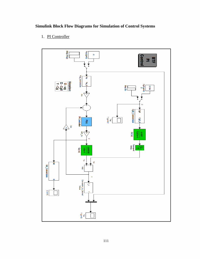
111
Simulink Block Flow Diagrams for Simulation of Control Systems
1. PI Controller

112
2. FB PI - FF Controller
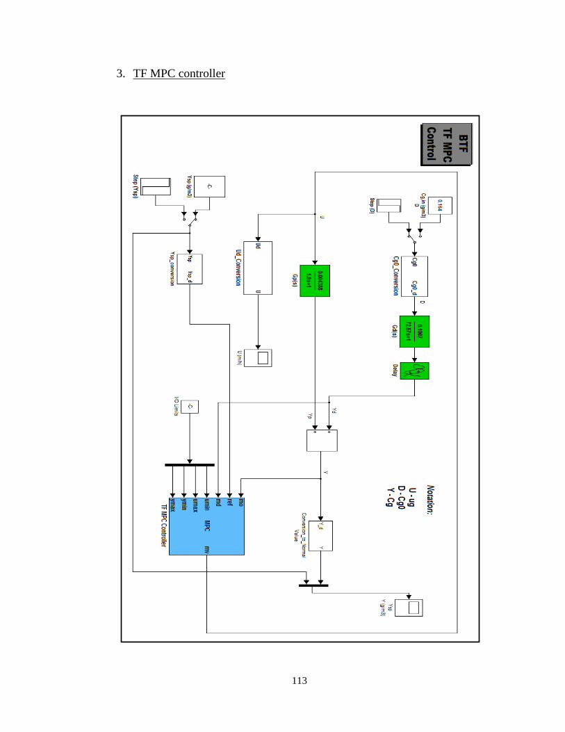
113
3. TF MPC controller
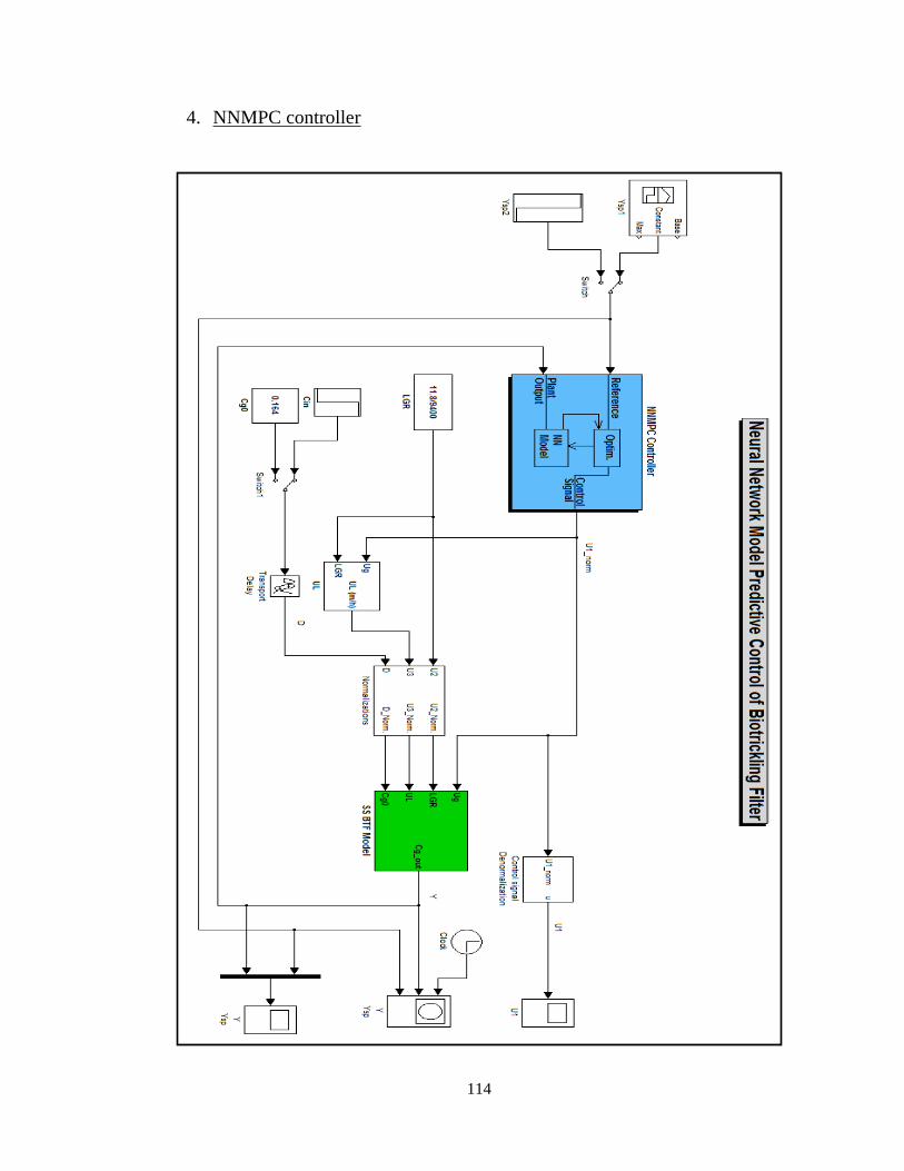
114
4. NNMPC controller
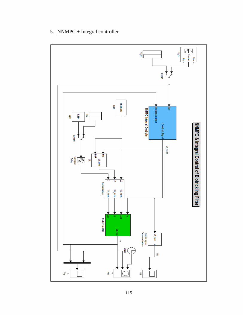
115
5. NNMPC + Integral controller
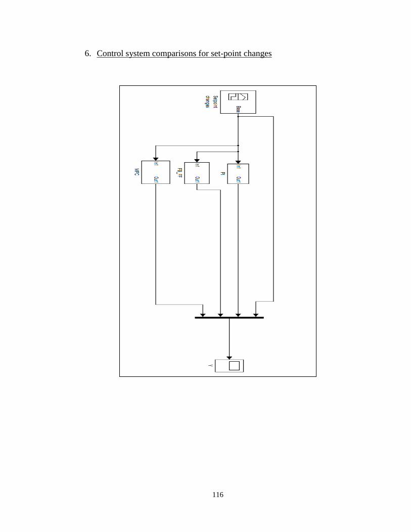
116
6. Control system comparisons for set-point changes
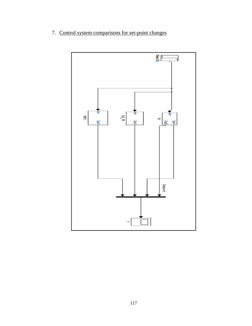
117
7. Control system comparisons for set-point changes

118
Vita
Originally from Pakistan, Wasim Ahmed Bashir was born on April 28, 1985, in
Dubai, United Arab Emirates. He started his primary education from an English school
with British Curriculum in Al Sadiq Islamic English School, conveniently located in the
city of Dubai. He successfully completed his O’ Level and graduated with top position in
2002. Aiming for further education, he enrolled in the English Medium School,
where he completed his A’ Level and graduated as a science student in 2005.
Mr Ahmed enrolled in American University of Sharjah and graduated cum laude
with a Bachelor of Science Degree in Chemical Engineering and a Minor in Engineering
Management in 2009. During his years as an undergraduate student, he received
academic scholarship and had been in the Dean’s list for four semesters. From his
undergraduate senior design collaborative project on biofilter process, he got to publish
two scholarly articles. In 2010, he continued to pursue his education by enrolling in a
Master’s program in Chemical Engineering at the American University of Sharjah. Under
the student assistantship program, he worked as a computer lab assistant at the university
for one year and then as a computer lab instructor for a computer methods undergraduate
course. He is expected to graduate in 2012.