MODELING PARTICLE FILTRATION AND CAKING IN FIBROUS …

Virginia Commonwealth University Virginia Commonwealth University

VCU Scholars Compass VCU Scholars Compass

Theses and Dissertations Graduate School

2011

MODELING PARTICLE FILTRATION AND CAKING IN FIBROUS MODELING PARTICLE FILTRATION AND CAKING IN FIBROUS

FILTER MEDIA FILTER MEDIA

Seyed Alireza Hosseini Virginia Commonwealth University

Follow this and additional works at: https://scholarscompass.vcu.edu/etd

Part of the Engineering Commons

© The Author

Downloaded from Downloaded from https://scholarscompass.vcu.edu/etd/2530

This Dissertation is brought to you for free and open access by the Graduate School at VCU Scholars Compass. It has been accepted for inclusion in Theses and Dissertations by an authorized administrator of VCU Scholars Compass. For more information, please contact [email protected].

http://www.vcu.edu/

http://www.vcu.edu/

https://scholarscompass.vcu.edu/

https://scholarscompass.vcu.edu/etd

https://scholarscompass.vcu.edu/gradschool

https://scholarscompass.vcu.edu/etd?utm_source=scholarscompass.vcu.edu%2Fetd%2F2530&utm_medium=PDF&utm_campaign=PDFCoverPages

http://network.bepress.com/hgg/discipline/217?utm_source=scholarscompass.vcu.edu%2Fetd%2F2530&utm_medium=PDF&utm_campaign=PDFCoverPages

https://scholarscompass.vcu.edu/etd/2530?utm_source=scholarscompass.vcu.edu%2Fetd%2F2530&utm_medium=PDF&utm_campaign=PDFCoverPages

mailto:[email protected]

http://www.graduate.vcu.edu/community/thesis.html School of Engineering

Virginia Commonwealth University

This is to certify that the dissertation prepared by Seyed Alireza Hosseini MODELING PARTICLE FILTRATION AND CAKING IN FIBROUS FILTER MEDIA has been

approved by his or her committee as satisfactory completion of the thesis or dissertation requirement for the degree of Doctor of Philosophy

Dr. Hooman Vahedi Tafreshi, School of Engineering Dr. Gary C. Tepper, School of Engineering Dr. P. Worth Longest, School of Engineering Dr. Vamsi K. Yadavalli, School of Engineering Dr. Rebecca Segal, College of Humanities and Sciences Dr. Gary C. Tepper, Chair of the Department of Mechanical and Nuclear Engineering Dr. Russell D. Jamison, Dean of the School of Engineering Dr. F. Douglas Boudinot, Dean of the School of Graduate Studies Jul. 11, 2011

2

© Seyed Alireza Hosseini 2011

All Rights Reserved

3

MODELING PARTICLE FILTRATION AND CAKING IN FIBROUS FILTER

MEDIA

A Dissertation submitted in partial fulfillment of the requirements for the degree of Doctor of Philosophy at Virginia Commonwealth University.

by

SEYED ALIREZA HOSSEINI MSc in Mechanical Engineering, Sharif University of Technology, Iran, 2008

BSc in Mechanical Engineering, University of Tehran, Iran, 2005

Director: HOOMAN VAHEDI TAFRESHI QIMONDA ASSISTANT PROFESSOR, DEPARTMENT OF MECHANICAL

ENGINEERING

Virginia Commonwealth University Richmond, Virginia

July 2011

iv

Acknowledgements

Foremost, I would like to express my sincere gratitude to my advisor Professor Hooman

Tafreshi for the continuous support of my Ph.D study and research, for his patience,

motivation, enthusiasm, and immense knowledge. His guidance helped me in all the time

of research. I could not have imagined having a better advisor and mentor for my Ph.D

study.

Besides my advisor, I would like to thank the rest of my thesis committee: Professor

Tepper, Professor Longest, Professor Segal, Professor Yadavalli, for their encouragement,

insightful comments, and hard questions.

This work has been supported by Virginia Commonwealth University and National

Science Foundation, CMMI NanoManufacturing Program (grant # 1029924).

My sincere thanks also go to Professor Edwards, for helping me about Analysis of

Variance part of my study. I also like to appreciate Professor Mossi for her efforts to

prepare a very friendly environment.

Last but not the least; I would like to thank my family: my parents, my wife, and my sister

for supporting me spiritually throughout my life. They always soften the life difficulties for

me. I owe all my achievements to them and I am happy to devote this work to them.

v

Table of Contents

Page

List of Tables ................................................................................................................... viii

List of Figures .................................................................................................................... ix

List of Symbols .............................................................................................................. xviii

Abstract ............................................................................................................................ xxi

Chapter

1 Introduction ....................................................................................................... 1

1.1 Background information ......................................................................... 1

1.2 Modeling Clean Filter Media ................................................................. 3

1.3 Single Fiber Loading ............................................................................ 17

1.4 Filter Clogging ...................................................................................... 24

2 Modeling Permeability of 3-D Nanofiber Media: Effects of Slip Flow ......... 33

2.1 Introduction .......................................................................................... 33

2.2 Virtual Nanofiber Media ...................................................................... 35

2.3 Flow Field Calculation ......................................................................... 36

2.4 Air Permeability of Nanofiber Media ................................................... 41

2.5 Conclusions .......................................................................................... 45

3 3-D Simulation of Particle Filtration in Electrospun Nanofibrous Filters Porous

Media .......................................................................................................... 50

3.1 Introduction .......................................................................................... 50

vi

3.2 Virtual Nanofiber Media .................................................................... 52

3.3 Flow Field Calculations ........................................................................ 53

3.4 Modeling Particle Capture in A Fibrous Medium ................................ 57

3.5 Results and Discussion ......................................................................... 60

3.6 Conclusions .......................................................................................... 64

4 Modeling Particle Filtration in Disordered 2-D Domains: A Comparison with

Cell Models ................................................................................................. 75

4.1 Introduction .......................................................................................... 75

4.2 Flow Field ............................................................................................. 77

4.3 Particle Flow and Capture .................................................................... 80

4.4 Results and Discussions ...................................................................... 84

4.5 Conclusions .......................................................................................... 89

5 On the Importance of Fibers’ Cross-Sectional Shape for Air Filters Operating in

the Slip Flow Regime .............................................................................. 105

5.1 Introduction ........................................................................................ 105

5.2 Governing Equations and Numerical Schemes .................................. 107

5.3 Results and Discussions ..................................................................... 111

5.4 Conclusions ........................................................................................ 116

6 Modeling Particle-Loaded Single Fiber Efficiency and Fiber Drag using Fluent

CFD Code ................................................................................................. 123

6.1 Introduction ........................................................................................ 123

6.2 Modeling Particle-Loaded Filter Media ............................................. 128

vii


6.4 Conclusions ........................................................................................ 141

7 Microscale 2-D Modeling of Instantaneous Dust Loading of Fibrous and

Pleated Filters ........................................................................................... 153

7.1 Introduction ........................................................................................ 153

7.2 Flow Field Calculations ...................................................................... 156

7.3 Modeling Dust Particle Deposition .................................................... 157


7.5 Modeling Instantaneous Pressure Drop of Pleated Filters .................. 167

7.6 Conclusions ....................................................................................... 171

8 Overall Conclusion ....................................................................................... 186

List of References ......................................................................................... 190

Curriculum vitae ........................................................................................... 198

viii

List of Tables Page

Table 3.1: Some of the existing single fiber efficacy expressions for particle capture due to

interception. 74


Brownian diffusion. 74


interception. 103


Brownian diffusion. 103


inertial impaction. 104

Table 7.1- Coefficients for equation 7.9. 184




ix

List of Figures Page

Figure 1.1- Interception capturing on a single fiber 31

Figure 1.2- Inertial impaction capturing on a single fiber 31

Figure 1.3- Inertial impaction capturing on a single fiber 31

Figure 1.4 – Collection efficiency of a filter due to different capturing regimes 31

Figure 1.5- Definition of cell model 32

Figure 1.6- Definition of interception efficiency 32

Figure 2.1: An example of our 3-D virtual nanofiber media with a fiber diameter of 100nm,

a thickness of 1.96 µm, and a SVF of 10% from two different views. 46

Figure 2.2: Simulation domain and the boundary conditions 47

Figure 2.3: Poiseuille flow in a 2-D duct 47

Figure 2.4: A comparison between the velocity profiles obtained for three different

Knudsen numbers of 0.001, 0.01, and 0.1 48

Figure 2.5: Effect of mesh density on our permeability calculations 48

Figure 2.6: Our numerical simulations with and without slip velocity boundary condition

are compared with the original and modified permeability expressions of Jackson and

James (1986) and Spielman and Goren (1968), as well as with the empirical correlation of

Ogorodnikov (1976), for a fiber diameter of a) 100 nm, b) 400 nm, c) 700 nm, and d) 1000

nm 49

Figure 3.1: An example of our 3-D virtual media with a fiber diameter of 100nm, a

thickness of 1.96 µm, and an SVF of 7.5%. 66

x

Figure 3.2: Simulation domain and boundary conditions are shown. Red spheres are placed

at the inlet to visualize the position at which the particles are injected. For the clarity of the

illustration only a few number of particles are shown. 67

Figure 3.3: Pressure drop as a function of mesh density around the circular perimeter of

fiber. The results are obtained for a medium with a fiber diameter of 400 nm and an SVF

of 4.95%. 68

Figure 3.4: An example of our particle concentration contour plots with 50pd nm= shown

in a plain slicing through a medium with a fiber diameter of 1000nm and an SVF of 7.5%.

Red to blue represents normalized particle concentration from 1 to 0. 68

Figure 3.5: a) an example of our particle trajectory tracking with 500pd nm= shown in a

plain slicing through a medium with a fiber diameter of 1000nm and an SVF of 7.5%, b)

magnified view of particle trajectory termination at a distance of / 2pd from the fibers.

Note that the spherical symbols in the figure do not represent the actual particle size and

are chosen for illustration only. 69

Figure 3.6: Pressure drop per unit thickness of different media with different SVFs and

fiber diameters are compared with the predictions of Davies (black lines) and Ogorodnikov

(red line) empirical correlations. Dashed-dotted line (-⋅-), long-dashed line (− −), solid line

(⎯), dotted line (⋅⋅⋅), dashed line (- -), and dashed-double-dotted line (-⋅⋅-), represent fiber

diameters of 1000 to 100 nanometers, respectively. 70

xi

Figure 3.7: Existing semi-empirical correlations for particle capture due to interception are

compared with one another and our simulation results for a filter with a fiber diameter of

100 nm and an SVF of 2.5. 71

Figure 3.8: Existing semi-empirical correlations for particle capture due to Brownian

diffusion are compared with one another and our simulation results for a filter with a fiber

diameter of 100 nm and an SVF of 2.5. 71

Figure 3.9: Total filter efficiency is calculated by adding our simulation results for particle

capture via Brownian diffusion and direct interception, and are compared with the

predictions of the expressions given by Liu and Rubow (1990), as an example. Note that

the SVFs of the results presented in this figure are approximate values with a 10% margin

of error from the stated values in the legend (i.e., 2.5%, 5.0%, and 7.5%). 72

Figure 3.10: Figure of merit is versus particle diameter for a) media with an SVF of 5.0%

but different fiber diameters, and b) media with a fiber diameter of 300nm but different

SVFs. 73

Figure 4.1: Flow chart of our disordered 2-D media generation algorithm. 90

Figure 4.2: An example of the simulation domains used for the simulations reported in this

work together with the boundary conditions. 91

Figure 4.3: Influence of mesh density on pressure drop calculations. The results are

obtained for a medium with a fiber diameter of 10µm and a volume fraction of 15%. 92

Figure 4.4: Influence of the domain size (number of fibers) on pressure drop calculations.

The results are obtained for a medium with a fiber diameter of 10µm and a volume fraction

of 15%. 92

xii

Figure 4.5: An example of our particle concentration contour plots with 50pd nm= shown

for a medium with a fiber diameter of 10µm and a volume fraction of 15%. Red to blue

represents normalized particle concentration from 1 to 0. 93

Figure 4.6: Mean square displacement calculated for an ensemble of particles having a

diameter of 100 nm suspended in quiescent air. 93

Figure 4.7: An example of our particle trajectory tracking with 50pd = nm shown for a

medium with a fiber diameter of 100 nm and a fiber volume fraction of 5%. Trajectories

are shown with (b) and without (a) the Brownian diffusion. 94

Figure 4.8: Influence of number of grid points around the perimeter of a fiber on collection

efficiency due to interception (a) and diffusion (b). The results are obtained for a fibrous

medium with a fiber diameter of 10µm and a fibers volume fraction of 15%. 95

Figure 4.9: Dimensionless pressure drop, ( )pf α , calculated for fibrous media having fiber

diameters of 10µm (a) and 100 nm (b) at different volume fractions of 5, 10, 15, and 20

percent. Predictions of the cell model of Kuwabara (1959), fiber array model of

Drummond and Tahir (1984), empirical correlations of Davies (1973), and Ogorodnikov

(1976), as well as the analytical expression of Jackson and James (1986) are also added for

comparison. A comparison is also made between the simulation results obtained with and

without the aerodynamic slip for the case shown in (b). 96

Figure 4.10: Diffusion Single Fiber Efficiency obtained from our CFD simulations are

compared with the predictions of existing semi-analytical correlations for media with a

xiii

fiber diameter of 10 µm but different fiber volume fractions of 5%, 10%, 15%, and 20%.

97

Figure 4.11: Interception Single Fiber Efficiency obtained from our CFD simulations is



98

Figure 4.12: Diffusion Single Fiber Efficiency obtained from our CFD simulations are


fiber volume fraction of 5% but different fiber diameters of 100, 400, 700, and 1000 nm,

respectively. 99

Figure 4.13: Interception Single Fiber Efficiency obtained from our CFD simulations is


fiber volume fraction of 5% but different fiber diameters of 100, 400, 700, and 1000 nm,

respectively. 100

Figure 4.14: Comparison between particle collection efficiency of aerosol filters modeled

using disordered 2-D and fibrous 3-D geometries. The fiber volume fraction is kept at 5%,

while the fiber diameter is varied from 100 nm to 1000 nm. 101

Figure 4.15: Comparison between single fiber efficiency due to inertial impaction obtained

from our disordered 2-D fibrous geometries and that of different expressions from

literature. Dashed line, solid line, and dashed-double-dot line represent expressions given

for low, medium, and high Stokes number regimes (Brown 1993). 102

xiv

Figure 5.1: Computational domain considered for modeling flow around square and

circular fibers. 118

Figure 5.2: Fiber drag in the no-slip and slip flow regimes are calculated for circular (a and

b), square (c and d), trilobal (e and f), and elliptical (g and h) fibers. For the case of circular

fibers, simulation results (symbols) are compared with the predictions of Equation (5.11)

(lines). Delta and solid line (—), square and dashed line (---), diamond and dash dotted line

(-.-), left triangle and dotted line (…), right triangle and long dashed line (– –), and

gradient and dash dot-dotted line (-..), represent solid volume fractions of 20%, 15%, 10%,

7.5%, 5%, and 2.5% , respectively. 119

Figure 5.3: Slip-to-no-slip fiber drag ratios are calculated for circular (a), square (b),

trilobal (c), and elliptical (d) fibers. For the case of circular fibers, simulation results

(symbols) are compared with the predictions of Equation (5.11) (lines). Delta and solid line

(—), square and dashed line (---), diamond and dash dotted line (-.-), left triangle and

dotted line (…), right triangle and long dashed line (– –), and gradient and dash dot-dotted

line (-..), represent solid volume fractions of 20%, 15%, 10%, 7.5%, 5%, and 2.5% ,

respectively. 120

Figure 5.4: Streamlines around circular (a and b), square (c and d), elliptical (e and f), and

trilobal (g and h) fibers in no-slip and slip flow regimes (i.e., microfiber and nanofibers,

respectively). Note how streamlines conform to the fiber’s perimeter in the slip flow

regime. 121

xv

Figure 5.5: Single fiber collection efficiency calculated for fibers with a diameter of 200

nm (a), 400 nm (b), 6 µm (c), and 8 µm (d), at a solid volume fraction of 10%. A

comparison is made between the efficiency of fibers with circular and square cross-

sections. 122

Figure 6.1: Simulation domain and the boundary conditions. 143

Figure 6.2: Flowchart of the particle loading subroutine (a) and the subroutine used for

resolving the spherical shape of the deposited particles (b). 145

Figure 6.3: Two particles with a diameter of 200 nm loaded on a fiber with a diameter of

1µm. The particles are made up of a group of cells marked using the procedure described

in Figure 6.2. Note that in generating this figure we have used a relatively fine mesh, for

better illustration. 146

Figure 6.4: Examples of particle dendrite formation of fibers with different diameters. a)

Dendrite formation in the interception-dominant regime (fiber and particle diameters are

4µm and 250nm, respectively, cell solidity is 5%), b) dendrite formation in the inertial

impaction regime (fiber and particle diameters are 20µm and 2000nm, respectively, cell

solidity is 3%), c) dendrite formation in the diffusion-dominant regime (fiber and particle

diameters are 1µm and 75nm, respectively, cell solidity is 5%) 147

Figure 6.5: Normalized single fiber efficiency during particle loading on a fiber with a

diameter of 1µm. Particle diameters are a) 75nm, b) 150nm, c) 250nm, and d) 500nm. 148

Figure 6.6: Normalized single fiber drag during particle loading on a fiber with a diameter

of 1µm. Particle diameters are a) 75nm, b) 150nm, c) 250nm, and d) 500nm. 149

xvi

Figure 6.7: An example of particle deposition in the inertial impaction regime. The fiber

and particle diameters are 20 and 2 microns, respectively, and the cell has a solidity of 3%.

a) Normalized single fiber efficiency, b) Normalized single fiber drag. 150

Figure 6.8: a) The b coefficient is plotted versus particle diameter. The values are taken

form the results shown in Figure 6.5. b) Clean fiber efficiency is plotted versus particle

diameters. Note the minimum clean fiber efficiency around a particle diameter of 75nm.

151

Figure 6.9: The h coefficient is plotted versus particle diameter. The values are taken from

the results shown in Figure 6.6. 152

Figure 7.1- An example of the simulation domains used for the simulations reported in this

work together with the boundary conditions. In this case 5fd mµ= , 7.5%SVF = . 173

Figure 7.2- Flow chart of particle loading in medium. 174

Figure 7.3- a) Streamlines passing through the loaded particles in medium have shown, b)

Particles are captured in flow domain as a collection of cells. 175

Figure 7.4- Loaded dendrites are shown in three different geometries all with 10fd mµ= :

a,b) depth & surface filtration ( 1pd mµ= , 2.5%SVF = ), c,d) depth & surface filtration

( 2pd mµ= , 2.5%SVF = ), e,f) depth & surface filtration ( 5pd mµ= , 7.5%SVF = ). 176

Figure 7.5- Effect of flow recalculation on results: a) normalized pressure drop b)

cumulative efficiency ( 5fd mµ= , 2pd mµ= , 2.5%SVF = ). 177

xvii

Figure 7.6- Increasing normalized pressure drop for variable SVFs: a,b) depth & surface

filtration compared with equations 7.9 and 7.10 respectively ( 10fd mµ= , 2pd mµ= ), c,d)

depth & surface filtration compared with equations 7.9 and 7.10 respectively ( 15fd mµ= ,

2pd mµ= ). 178

Figure 7.7- Increasing cumulative efficiency for variable SVFs compared with equation

7.11: a) 10fd mµ= , 2pd mµ= , b) 15fd mµ= , 2pd mµ= . 179

Figure 7.8: Dust cake deposition pattern and air streamlines inside rectangular and

triangular pleats with a) 4 pleats per inch, b) 20 pleats per inch, c) 15o pleat angle, and d) 4o

pleat angle. Particle diameter and flow velocity are 3µm and 0.2 m/s, respectively. 180

Figure 7.9: Pressure drop increase during particle loading with rectangular and triangular

pleats for particles with diameters of 3 and 10µm and air inlet velocities of 0.2 and 1m/s.

181

Figure 7.10: Dust cake deposition pattern and air streamlines inside filters with 15

rectangular or triangular pleats per inch loaded with particles having 3 and 10µm diameters

with air velocities of 0.2 and 1 m/s. 182

Figure 7.11: Comparison between the pressure drop increase for filters with 15 rectangular

and triangular pleats per inch loaded with particles having 3 and 10µm diameters with air

velocities of 0.2 and 1 m/s. 183

xviii

List of Symbols

a y-intercept of the line from curve fitting to normalized single fiber efficiency data b slope of the line from curve fitting to normalized single fiber efficiency data

rC Correction factor d pleat distance

fd Fiber diameter

md Collision diameter

pd Particle diameter D Diffusion coefficient E single fiber efficiency of loaded fiber or filter

0E single fiber efficiency of clean fiber or filter E∑ Total SFE

dE SFE due to Diffusion

RE SFE due to Interception f Dimensionless permeability

df Dimensionless pressure drop or (fiber drag)

lf Dimensionless force per unit fiber length

iG random number h Filter Thickness H Height of Poiseuille channel k Permeability

0K Modified 2nd kind Bessel functions of order zero

1K Modified 2nd kind Bessel functions of order one

fKn Fiber Knudsen number

gKn Gap Knudsen number

pKn Particle Knudsen number k Permeability

Davk Permeability correlation of Davies (1973) sJJk Modified permeability expression of Jackson & James (1986)

KCk Kozeny-Carman permeability

Ogok Permeability correlation of Ogorodnikov (1976) layIPk layered in-plane structure permeability layTPk layered through-plane structure permeability isok 3-D isotropic structure permeability

xix

Ku Kuwabara hydrodynamic factor l fiber length L Inlet region length or Pleat height M loaded mass per unit volume n Normal non-dimensional position vector

( )in t Brownian force per unit mass in the x-direction ( )jn t Brownian force per unit mass in the y-direction

N Particle concentration AN Avogadro’s number

P Penetration Pe Peclet number p Pressure p∆ pressure drop across the loaded filter

0p∆ pressure drop across the clean filter

nsp∆ No-slip pressure difference

sp∆ Slip pressure difference q curve fitting coefficient r Fiber radius R particle to fiber diameter ratio R Ideal gas constant Re p particle's Reynolds number S spectral intensity t Time T Temperature

inu inlet velocity of pleated filter u Average velocity in the x-direction

maxu Maximum velocity in the x-direction

wu Wall slip velocity U Filter’s face velocity

1U random numbers

2U random numbers u Fluid velocity in the x-direction

pu Particle velocity in the x-direction

wu Fluid velocity at the wall v Fluid velocity in the y-direction

iv relative field velocity vector

ipv relative particle velocity vector

xx

pv Particle velocity in the y-direction w Fluid velocity in the z-direction

pw Particle velocity in the z-direction α Solid Volume Fraction, Solidity, Or Packing density of filter β coefficient in normalized pressure drop equation δ coefficient for predicting filter efficiency ε porosity γ empirical collection efficiency raising factor θ half of the pleat angle λ Mean free path µ Viscosity ν kinematic viscosity

pρ particle density = 1000 kg/m3

σ Boltzman constant ( 122231038.1 −−−× Kkgsm )

vσ Tangential momentum accommodation coefficient

wτ Wall shear stress ξ coefficient for predicting filter efficiency

xxi

Abstract

MODELING PARTICLE FILTRATION AND CAKING IN FIBROUS FILTER MEDIA

By Seyed Alireza Hosseini, MSc

A Dissertation submitted in partial fulfillment of the requirements for the degree of Doctor of Philosophy at Virginia Commonwealth University.

Virginia Commonwealth University, 2011

Major Director: Dr. Hooman Vahedi Tafreshi Qimonda Assistant Professor, Department of Mechanical and Nuclear Engineering

This study is aimed at developing modeling methodologies for simulating the flow of air

and aerosol particles through fibrous filter media made up of micro- or nano-fibers. The

study also deals with modeling particle deposition (due to Brownian diffusion,

interception, and inertial impaction) and particle cake formation, on or inside fibrous

filters. By computing the air flow field and the trajectory of airborne particles in 3-D

virtual geometries that resemble the internal microstructure of fibrous filter media, pressure

drop and collection efficiency of micro- or nano-fiber filters are simulated and compared

with the available experimental studies. It was demonstrated that the simulations

conducted in 3-D disordered fibrous domains, unlike previously reported 2-D cell-model

simulations, do not need any empirical correction factors to closely predict experimental

xxii

observations. This study also reports on the importance of fibers’ cross-sectional shape for

filters operating in slip (nano-fiber filters) and no-slip (micro-fiber filters) flow regimes. In

particular, it was found that the more streamlined the fiber geometry, the lower the fiber

drag caused by a nanofiber relative to that generated by its micron-sized counterpart.

This work also presents a methodology for simulating pressure drop and collection

efficiency of a filter medium during instantaneous particle loading using the Fluent CFD

code, enhanced by using a series of in-house subroutines. These subroutines are developed

to allow one to track particles of different sizes, and simulate the formation of 2-D and 3-D

dendrite particle deposits in the presence of aerodynamic slip on the surface of the fibers.

The deposition of particles on a fiber and the previously deposited particles is made

possible by developing additional subroutines, which mark the cells located at the

deposition sites and modify their properties to so that they resemble solid or porous

particles. Our unsteady-state simulations, in qualitative agreement with the experimental

observations reported in the literature, predict the rate of increase of pressure drop and

collection efficiency of a filter medium as a function of the mass of the loaded particles.

1

CHAPTER 1. Introduction 1. Background Information

1.1 Filter Structure

The structure of filters is the most fundamental of their properties to be considered. The

principal filter types can be divided into membrane filters, granular filters, foam filters, and

fibrous filters. Using fibrous filters is the most common method of removing particles from

gas streams. Fibrous filters are divided into two main categories: nonwoven and woven

filtration media. This thesis’ aim is to study the nonwoven fibrous filter.

1.1.1- Nonwoven Filtration Media

A nonwoven material can be defined as, “a sheet, web, or mat of natural or manmade

fibers or filaments that have not been changed into yarns and that are bonded to each other

by any of several means” (INDA 1999).

Hutten has defined it as, “A nonwoven filter medium is a porous fabric composed of a

random array of fibers or filaments and whose specific function is to filter and/or separate

phases and components of a fluid being transported through the medium or to support the

medium that does the separation”(Hutten, 2007).

Nonwoven filters have different applications in Automotive, Food and Beverages, power

generation, transportation, electronic, water treatment, chemical, pulp and paper, toiletries

and cosmetic, mining and mineral, pharmaceutical, and biological industry. As an

example, HEPA (high efficiency particulate air) which is one of the high efficiency

nonwoven filters has been explained in next chapter.

2

1.1.2- HEPA Filters

HEPA filters are composed of a mat of randomly arranged fibers. The fibers are typically

composed of fiberglass and possess diameters between 0.5 and 2.0 micrometer. The

common assumption that a HEPA filter acts like a sieve where particles smaller than the

largest opening can pass through is incorrect. Unlike membrane filters where particles as

wide as the largest opening or distance between fibers cannot pass in between them at all,

HEPA filters are designed to target much smaller pollutants and particles. HEPA filters

have different applications. HEPA filters can be used to remove airborne bacterial and viral

organisms and, therefore, infection. Typically, medical-use HEPA filtration systems also

incorporate high-energy ultra-violet light units to kill off the live bacteria and viruses

trapped by the filter media. Some of the best-rated HEPA units have an efficiency rating of

99.995%, which assures a very high level of protection against airborne disease

transmission. HEPA filters are the last part of filtration in clean rooms. HEPA filter can be

used in vacuum cleaners as it traps the fine particles (such as pollen and dust mite feces)

which trigger allergy and asthma symptoms. HEPA filters also can be used as cabin air

filter in cars, planes, or trains. Modern airliners use HEPA filters to reduce the spread of

airborne pathogens in recirculated air. Test results showed that bacteria and fungi levels

measured in the airplane cabin are similar to or lower than those found in the common

home. These very low microbial contaminant levels are due to the complete exchange of

inside cabin air 10 to 15 times per hour and the high filtration capability of the

recirculation system.

3

1.1.3- Nonwoven Filter Parameters

Nonwoven filter parameters are fiber diameter, fd , Solid Volume Fraction, SVF , and

filter thickness, t . Fiber diameter in this study covers a wide range from nanofibers to

micro fibers. Thickness, t , of a filter depends on number of layers, but in this study it does

not pass 1mm due to simulation limitations. SVF or α , is the ratio of filter volume which

is filled up by fibers. SVF, in this study has a wide range from 2.5% to 15%.

1.2 Modeling Clean Filter Media

1.2.1 Evaluation of Filtration Performance

The major parameters in characterizing filtration performance are pressure drop and

collection efficiency. Collection efficiency is the fraction of particles that get trapped by a

filter and is defined as:

in out

in

N NEN−

= (1.1)

where N is the number of particles. Another useful term is penetration which means

fraction of particles that leave the media:

out

in

NPN

= (1.2)

These equations can also be defined in terms of concentration of the particles. Penetration

and efficiency are related to one another as:

1P E= − (1.3)

4

It is known that a filter's collection efficiency increases by increasing Solid Volume

Fraction or decreasing fiber diameter. This, unfortunately, leads to an increase in the

medium's pressure drop and makes it difficult to judge whether or not a filter has been

designed properly. To circumvent this problem, Figure of Merit (also referred to as Quality

Factor) is often used in industry:

ln PFOMp

= −∆

(1.4)

A good filter is one which has a high efficiency and a low pressure drop or simply a high

FOM.

1.2.2 Aerosol Filtration

Aerosol filtration refers to removal of solid and liquid particles from suspended air. There

are four basic mechanisms by which an aerosol particle can deposit on a neutral fiber in

aerosol filtration. These are interception, inertial impaction, Brownian diffusion, and

gravitational settling (negligible in the case of nanoparticles). Interception efficiency

means particle is intercepted by a fiber when the distance from the center of mass of the

particle to the fiber surface is equal or less than the radius of the particle. Figure 1.1 shows

an image of interception capturing on a single fiber.

In case of heavier particles, they will deviate from their original streamlines and touch the

fibers. According to (Hinds, 1999) as “a particle, because of its inertia, is unable to adjust

quickly enough to the abruptly changing streamlines near the fiber and crosses those

5

streamlines to hit the fiber”. Figure 1.2 shows an image of inertial impaction capturing on a

single fiber.

Brownian motion is the random movement of particles suspended in a fluid (i.e. a liquid

such as water or air). Efficiency calculated based on random Brownian motion is also

called diffusion efficiency. Diffusion efficiency is more important in the case of small

particles. Figure 1.3 shows an image of diffusion capturing on a single fiber

The collection efficiency of a fibrous fiber is defined as a ratio of trapped particle to all

entering particles. Figure 1.4 shows the related efficiencies due to different mentioned

procedures. It is obvious that diffusion is the governing regime for small particle

deposition and interception effects become important as the size of particle increases and

for the case of heavy big particles inertial impact is the governing regime. By adding these

effects the collection efficiency has a v- shape. The minimum of this curvature is called the

most penetrating size of the particle which shows that the filter has the lowest efficiency to

capture this special particle size.

1.2.3 Single Fiber Theory

Knowing how particles deposit on a single fiber, one can predict the performance of a

filter. Efficiency of a filter medium can be obtained in terms of its thickness, solid volume

fraction, and fiber diameter if the total Single Fiber Efficiency (SFE), E∑, is available.

Efficiency of a fibrous filter is given as (Brown, 1993):

41 exp( )

(1 )f

E tE

dα

π α∑−

= −−

(1.5)

6

The total SFE, E∑, is the sum of SFEs due to interception, inertial impaction, and Brownian

diffusion. Inertial impaction for low-speed submicron particles is relatively small and often

negligible. The total SFE is given as (Brown, 1993):

1 (1 )(1 )(1 )R d IE E E E∑ = − − − − (1.6)

where RE , dE , and IE are single fiber efficiency due to interception, Brownian diffusion,

and inertial impaction, respectively.

1.2.4 Cell Model

Cell model means a fiber of radius fR surrounded by an imaginary circle with the same

center. The circle radius b is defined in a way to give the true SVF.

2

2

fRSVF

b= (1.7)

The geometry has been shown in figure 1.5. The cell model method has a very simple

geometry of just one fiber in a finite space instead of an infinite space of isolated fiber

models. For this reason, the effects of other fibers are taken into account. Although it is a

very simplified version of real geometry; this suggested method by Kuwabara (1959) and

Happel (1959) gives us an acceptable prediction. It also assumes that all fibers in the filter

have the same flow field and they are perpendicular to main flow direction. As it was the

only approach for solving fluid flow; this result was used for decades after that by Davies

(1973), Lee and Liu (1982a), Brown (1984), Brown (1989), Brown (1998). By using this

geometry Kuwabara solved two dimensional viscous flow equations and obtained the

7

velocity profile around fiber. In Kuwabara cell model the stream function ψ can be

obtained by solving the biharmonic equation in cylindrical polar coordinate:

4 0ψ∇ = (1.8)

The simplest solution is:

3( ln )sinBAr Cr r Drr

ψ θ= + + + (1.9)

where A, B, C, D are constants, which will be specified by using boundary conditions. By

having streamlines from the Kuwabara model, predicting interception efficiency by

assuming the particle follows the same path as the streamline is possible. The interception

efficiency is the ratio of limiting streamlines of the flow to the fiber diameter as it is shown

in figure 1.6.

R

f

yR

η = (1.10)

For any point on the cell, we have vyψ = . So by substituting this in equation 1.10, the

interception efficiency is calculated as:

R

fvRψη = (1.11)

Let 2πθ = and f pr R R= + in the stream function, Kuwabara (1959) obtained:

2 21 12ln(1 ) 1 ( ) (1 ) (1 )2 1 2 2R

RE R RKu R

α αα+ ⎡ ⎤= + − + + − − +⎢ ⎥+⎣ ⎦ (1.12)

8

in which p

f

RR

R= , is a dimensionless number which is called interception parameter and

Ku is Kuwabara number which is defined as 225.075.0ln ααα −+−−=Ku and α is SVF. The

above equation is hard to calculate. A new equation calculated by Lee and Liu (1982a) by

using equivalent series of the above equation can be used. They actually considered the

first term of that series as:

21(1 )R

REKu Rα−

=+

(1.13)

Due to the complicated geometry of fibrous media, the above equation does not match with

experimental result so a new empirical coefficient should be added to make the formula

valid with experiments. By comparison with the experimental result a 0.6 coefficient is

added to this equation. More details about this comparison and the way that Liu and

Rubow (1990) modified equation 1.13 to reach equation 1.14 are given in the next chapter.

210.6(1 )R r

RE CKu Rα−

=+

(1.14)

Liu and Rubow (1990) modified this equation again by multiplying a new coefficient, rC ,

for considering the slip effect. rC is a function of fkn as following:

210.6(1 )

1.9961

R r

f

r

RE CKu R

knC

R

α−=

+

= +

(1.15)

9

1.2.5 Brownian Diffusion

Particles deviate from their streamlines due to Brownian motion. This can be quantified by

using the coefficient of diffusion. By using an average displacement of a particle from its

original location in any direction, the following equation is obtained by Einstein:

2 2x Dt= (1.16)

D is the coefficient of diffusion which is a linear function of temperature as:

/ (3 )c pD C T dσ πµ= (1.17)

in which 1.1/1 (1.257 0.4 )pKn

c pC Kn e−= + + is the empirical factor of Cunningham for slip

correction at the surface of nanoparticles and 23 2 2 11.38 10 ( )m kg s Kσ − − −= × is the

Boltzmann constant. T and µ are the air temperature and viscosity, respectively, while

Pd is the particle diameter.

For calculating filter efficiency analytically, the convective-diffusive equation for the

concentration of the small particles based on the Eulerian approach can be solved.

2 2 2

2 2 2( )N N N N N Nu v w D

x y z x y z∂ ∂ ∂ ∂ ∂ ∂

+ + = + +∂ ∂ ∂ ∂ ∂ ∂

(1.18)

Different solution methods for equation 1.18 have been suggested by scientists to calculate

diffusion efficiency. Natanson (1957) proposed a formula that is not a good approximation

because of neglecting effects of other neighboring fibers. Or in another words, they used an

isolated fiber method in infinite space.

Stechkina and Fuchs (1966) suggested a formula, which is calculated by the boundary

layer analysis, valid for Pe>100. This method does not cover virtual neighboring fibers,

10

but by assuming cell model and by using Kuwabara flow field it simplifies effects of other

neighboring fibers. Modified Stechkina formula also was suggested later with a smaller

multiplying coefficient.

Lee and Liu (1982a) solved a convective-diffusive equation for the concentration of the

particles based on the Eulerian approach in polar coordinates as follows:

2 2

2 2 2

1( )r

un n n n nu Dr r r r r r

θ

θ θ∂ ∂ ∂ ∂ ∂

+ = + +∂ ∂ ∂ ∂ ∂

(1.19)

The above equation is solved analytically by neglecting the last term. By including the

factor of 1 α− in the numerator and using the hydrodynamic factor which is proposed by

Kuwabara in the denominator, a new hydrodynamic factor was introduced as

(1 ) / Kuξ α= − . The results can be applied over a wider range of SVF by using this new

hydrodynamic factor instead of the older one, 1/ Kuξ = . Finally, the following formula

suggested by Lee and Liu (1982a) based on theoretical solution.

1/3

2 312.6DE PeKuα −−⎛ ⎞= ⎜ ⎟

⎝ ⎠ (1.20)

In which Pe is the Pecklet number /fPe U d D= . This equation does not match with the

experiment so the equation is modified by inserting the new coefficient. Lee and Liu

(1982a) could only measure total efficiency by neglecting inertial impaction efficiency in

the range of most penetrating particle sizes. So, the interception formula and the diffusion

formula added together with variable coefficients can be compared with experimental

results to obtain a new empirical formula. By using the new nondimensional parameters

11

instead of totE , / 1totE PeR R+ is compared to 13 1

31 / 1Pe R R

Kα−⎛ ⎞ +⎜ ⎟

⎝ ⎠ . By using this new

parameter, total efficiency effects are assigned to diffusion when it is smaller than 0.3 and

to interception when it is greater than 3. The middle range, fortunately, has both effects of

diffusion and interception so it can not be used to predict these coefficients. The following

equation suggested by Lee and Liu (1982a) for diffusion:

1/3

2 311.6DE PeKuα −−⎛ ⎞= ⎜ ⎟

⎝ ⎠ (1.21)

The experimental results which are used by equation 1.21 to modify analytical expressions

are based on a 11.0 mµ fiber diameter and SVFs of 0.0086, 0.0474, and 0.151 which are

far from nano scale fibers inspected in this study.

On the other hand equation 1.21 with no slip boundary condition underestimates the

diffusion efficiency of nanofibers. The modified Liu and Rubow equation (1990) accounts

for slip boundary condition by a slip correction factor, but the fiber diameter range does

not cover smaller than 100nm. Liu and Rubow (1990) suggested following equation:

1/3

2 3

,

13

11.6

(1 )1 0.388 ( )

d Liu d

d f

E Pe CKu

PeC KnKu

α

α

−−⎛ ⎞= ⎜ ⎟⎝ ⎠

−= +

(1.22)

Rao and Faghri suggested using numerical methods as it could separate the effects of

diffusion and interception in total efficiency, eliminating the difficulty of separating effects

of the two, as well as providing the capability of analyzing the effects separately. For

12

assuming the effects of other fibers, an in-line or staggered two dimensional tube bank is

assumed. The Navier-Stokes equations are solved first numerically by using the finite

volume method developed by patankar (1980) and then the equation 1.19 is solved for

diffusion. So there is still a lack of a real virtual model. Their results were compared by

Stechkina and Fuchs (1966), Kuwabara (1959), and Lee and Liu (1982 b) for R<0.5.

Finally, two different formulas are suggested depending on the Peclet range, one for Pe<50

and the other for 100<Pe<300. Also, another equation is suggested by Payet et al. (1991)

for slip flow.

1/3

2 3 '

,

,

11.6

11

d Payet d d

d

d Liu

E Pe C CKu

CE

α −−⎛ ⎞= ⎜ ⎟⎝ ⎠

=+

(1.23)

dC in equation 1.23 is the same as in equation 1.22.

1.2.6 Inertial Impaction

Inertial impaction happens because of deviation of particle from streamlines due to inertia.

Since a particle can not adjust its path due to streamline curvatures, it impacts the fiber due

to its inability to avoid it. By applying drag force on a particle, the particle motion equation

is:

3 p

dvm d vdt

πµ= − (1.24)

13

By solving this first order differential equation, the stopping time, sτ , the time required for

its velocity to drop by a factor of e, and its stopping distance, sd , the distance it travels

before coming to rest, are calculated as:

2

18p

s

d ρτ

µ= (1.25)

2

18p

s

vdd

ρµ

= (1.26)

The effect of inertial impaction has been studied by using the nondimensional Stokes (Stk)

number. By substituting u from v in equation 1.26, the parameter describing the behavior

of a particle suspended in an air stream is calculated. In order to have a nondimensional

number, sd is divided by the characteristic length of the fiber which is the fiber diameter.

2

18p

f

UdStk

dρ

µ= (1.27)

The inertial impaction regime can be divided into three different categories of low,

medium and high Stokes number. An expression for calculating the single fiber efficiency

of low Stokes number is calculated as:

24I

J StkEKu×

= (1.28)

In which J is defined as:

0.62 2.8(29.6 28 ) 27.5J R Rα= − − (1.29)

In the case of a high Stokes number, the particle stream lines will be straight and the

velocity of the particle will be equal to the initial velocity of the air. After modifying

14

equation 1.24, by substituting v u− instead of v , it can be solved easily. This is the first

order perturbation theory. Finally, the inertial impaction for the case of a high Stokes

number is:

1IEStkµ

= − (1.30)

where the constant µ equals 0.805 for a SVF of 5% by using Kuwabara field. In the case of

medium Stokes numbers curve fitting should be used which suggests:

3

3 20.77 0.22I

StkEStk Stk

=+ +

(1.31)

1.2.7 Air Permeability and Slipping Effect

Depending on the fiber diameter and gas thermal conditions, continuum flow regime

( 310fKn −< ), slip-flow regime ( 310 0.25fKn− < < ), transient regime ( 0.25 10fKn< < ), or

free molecule regime ( 10fKn > ) can prevail inside a fibrous medium. Here,

2 /f fKn dλ= is the fiber Knudson number where 2/ ( 2 )a mRT N d pλ π= is the mean free

path of gas molecules. Air flow around most electrospun nanofibers is typically in the slip

or transition flow regimes. Slip velocity is permitted to occur at the fiber surface, as is

expected for flows with non-zero Knudsen numbers. This has been done by defining the

wall shear stress using the Maxwell first order model (McNenly et al., 2005; Duggirala,

2008):

2 vw

wv

uun

σ λσ− ∂

=∂

(1.32)

15

To allow slip to occur, the above equation 1.32 can be used as the shear stress at the wall

using following equation:

2v

w w

v

uσµτλ σ

=−

(1.33)

The greater the slip velocity, the closer the streamlines are to the fiber surface (Maze et al.

2007). This means that the greater the slip velocity, the lesser the influence of the fibers on

the flow field. Therefore, it is expected (and experimentally observed) that permeability of

a nanofiber medium is greater than what traditional permeability models predict. In almost

all permeability models, permeability of a fibrous material is presented as a function of

fiber radius, r, and Solid Volume Fraction (SVF),α , of the medium. There are several

equations available for estimating permeability. For example, analytical expressions of

Jackson and James (1986), developed for 3-D isotropic fibrous structures, and that of

Spielman and Goren (1968), developed for through-plane permeability of layered 3-D

media, given, respectively, as:

23 [ ln( ) 0.931]20

rk αα

= − − (1.34)

and

( )( )

1

0

/1 5 13 6 4α/

K r kk+ =r K r k

(1.35)

In the above equation, 0K and 1K are the modified 2nd kind Bessel functions of orders zero

and one, respectively. Permeability (or pressure drop) models obtained using ordered 2-D

16

fiber arrangements are known for under-predicting the permeability of a fibrous medium

(Wang et al., 2006a; Zobel et al., 2007; and Jaganathan et al., 2008a).

Here, we define our correction factor as snsr ppC ∆∆= / to be used in modifying the original

permeability expressions of Jackson and James (1986), Spielman and Goren (1968), and/or

any other expression based on the no-slip boundary condition, in order to incorporate the

slip effect. For instance, the modified expression of Jackson and James (1986) can be

presented as:

23 [ ln( ) 0.931]20

s

JJ r

rk Cαα

= − − (1.36)

It is worth mentioning that our extensive literature search for an explicit expression

capable of predicting the permeability of nanofibrous media only resulted in an empirical

correlation obtained by Ogorodnikov in 1976. The correlation of Ogorodnikov (1976) was

obtained by fitting a curve into experimental data in the slip and transition regime.

2 4( 0.5 0.5ln 1.15 (1 ) )4

f

Ogo

r knk

α αα

− − + −= (1.37)

Another popular equation is the empirical correlation of Davies (1973):

( )( ) 12 3/2 364 1 56Dav fk d α α

−

= + (1.38)

Based on Darcy’s law ( / )k Ut pµ= ∆ , Permeability, k, can be used to find pressure drop.

So it seems useful to talk about pressure drop in this part as well. A filter’s pressure drop

depends on the air viscosity, filter thickness, flow face velocity (here 0.1m/s unless

otherwise stated), fiber diameter, and solid volume fraction, as:

17

2( )d

f

p Vft d

µα∆= (1.39)

Where dimensionless pressure drop, ( )df α , is only a function of solid volume fraction,

and has different forms based on different theories. For the Kuwabara cell model, ( )df α is

given as:

16( )df Kuαα = (1.40)

Drummond and Tahir (1984) proposed 2 1( ) 32 ( ln 1.476 2 1.774 )df α α α α α −= − − + − . Note

that the latter and Kuwabara expressions are derived for ordered 2-D fibrous geometries.

Ordered 2-D geometries tend to over-predict the pressure drop of a real (i.e., 3-D) fibrous

geometry (Natanson, 1957). Disordered 2-D fibrous geometries, however, tend to result in

pressure drop values somewhere between those of ordered 2-D and disordered 3-D media

like the Davies equation.

1.3 Single Fiber Loading

Existing theories of particle filtration are developed for clean filter media. These theories

are based on a solution of the flow field around a perfectly clean fiber and have resulted in

simple expressions for calculating the collection efficiency and pressure drop of filter

media (see Brown 1993 for a review). Obviously, filters do not remain clean during the

course of their operation. Particles deposit on the fibers and form dendrite structures with

complicated geometries. These deposited particles affect the flow field around the fiber

and render the abovementioned expressions inaccurate. The existing expressions are,

18

therefore, valid only for the early stages of a filter’s lifecycle. As a filter starts collecting

airborne particles, its performance begins to deviate from the models’ predictions. Despite

its industrial importance, filtration science has not yet sufficiently developed to provide

accurate predictions for the performance (pressure drop and collection efficiency) of

particle-loaded filter media.

There are different models for capturing particle efficiency via numerical methods. If we

start by assuming filter fibers uniformly get thicker as a rough estimation, we run into

problems. For example, by using available equations of clean fibrous material, the pressure

drop would approximately double if we assume the dust load has the same volume as the

fiber. However, the rate of pressure drop increase by loading the same mass in a real filter

is much higher than this. In some cases, by capturing 1% of solid volume fraction, the

pressure drop is doubled (Smissen, 1971).

A realistic model of loading process should capture the dendrite shape of the particle

deposits. The shape of a loaded fiber changes depending on the particle deposition regime.

If the deposition mechanism is mainly interception, the deposit pattern will be on the

fibers’ lateral sides. By increasing the Stokes number, the mode of particle deposition

changes to inertial impaction. In this case, the particle does not follow the streamlines

perfectly and instead travels on a straight path and so deposit on the fiber’s front side. Note

that particles which are deposited on the lateral sides cause a much higher pressure drop

than those deposited on the fiber front side. Particle deposition due to Brownian diffusion

19

is believed to form uniform deposits all around the fiber, as the inertial effects are

negligible.

Watson (1946) was the first to observe loading on a single fiber but he did not report any

quantitative experimental results. Billings in 1966 attempted to formulate loading on a

single fiber. By using SEM micrographs with constant loading time intervals, he counted

the number of loaded particles to suggest an empirical correlation in terms of /N S as a

parameter in which N is the number of loaded particle and S is the fiber surface area:

0 . NCS

η η= + (1.41)

Billing’s experiments were based on 0.1 0.35Stk = − and 0.13R ≈ . Payatakes and Tien

(1976) proposed a theoretical model based on the assumption that particle chains grow in

orderly patterns in a Kuwabara flow field (assuming no interaction occurs between the

dendrites) and a particle is only collected by interception. This model came nowhere close

to predicting true experimental results. Later on, Payatakes and Gradon (1980) modified

this model to capture diffusion and inertial impaction effects. A general theory was later

suggested by Tien et al. (1977). However, the theory of Tien et al. (1977) could not

produce any quantitative information. Barot (1980) predicted increased efficiency when a

number of particles are injected in the media for Stk numbers varying from 0.1 to 0.7.

Barot suggested predicting the efficiency based on the derivative of the number of particles

with respect to time as he obtained a concave upward curvature:

20

1

f

dNd LUC dt

η = (1.42)

in which 0/dN dNη = .

Kanaoka et al. (1980) proposed new single fiber efficiency formulas. By using Monte

Carlo simulations in Kuwabara’s cell model and calculating efficiency for different Stokes

numbers and interception parameters, the ratio of single fiber efficiency of loaded-to-clean

fiber was approximated with a linear function of trapped mass in a unit filter volume:

0

( ) 1m mη λη

= + (1.43)

where 0η is the efficiency of the bare fiber, λ is an empirical collection efficiency raising

factor, and m is the accumulated mass per filter volume in 3/kg m . In some studies m has

been assumed to be mass per unit fiber length. The Monte Carlo simulation technique was

used to express the growth of particle dendrites on a fiber in Kuwabara's cell (Kanaoka et

al., 1980). The simulation results were used to obtain a rough estimation ofλ , collection

efficiency raising factor, by using equation 1.43. Although this equation seems like an easy

linear equation, it is not very useful. The complexity of this equation is hidden inλ , as it is

too hard to find a unique equation for λ based on filtration nondimensional numbers like

Stk, R, and Pe. The coefficient of the linear function,λ , decreases as the Stokes number

and interception parameter increase. Kanaoka et al. (1980) used the analytical solution of

Kuwabara (1959) to calculate particle trajectories and simulate the efficiency of their

media. In their work, however, flow field was not updated during the particle deposit

21

formation, which could result in overestimation of collection efficiency. This is due to the

fact that the streamlines change in response to the changes in the filter’s morphology

caused by particle deposition. As will be discussed later in the current section, flow field

should be updated during the deposit formation as frequently as possible, to correctly

simulate the instantaneous flow field in a filter medium. In Kanaoka et al. (1980)

calculations, each deposited particle is considered by marking one cell of the medium so

that the same mesh cannot be used for different particle sizes. The qualitative shape of the

dendrite is fairly similar to the real model. There are a few other studies reported in

literature on modeling pressure drop and collection efficiency of particle loaded media,

each suffering from some simplifying assumptions.

Emi and Kanaoka (1984) conducted additional experiments to validate their suggested

theoretical equation 1.43. Their particles were large enough to limit the capture

mechanisms to inertial impaction and interception. In these experiments, they found

contradictory results in respect to their older published work in 1974, which found no

sensitivity in predicting efficiency by varying the interception parameter. However, the

collection raising factor was found to decrease from 10 to 0.1 3 /m kg , the same trend as

was reported in their older publication.

Renbor et al. (1999) investigated the single fiber efficiency at critical values of the Stokes

number. They considered the effect of adhesion efficiency. Their experimental results

show that the filtration velocity can not be increased to obtain higher efficiency. By

22

reaching a critical Stokes number the single fiber efficiency decrease substantially. In their

study, Stokes number varies in the range of 0.8-5.0. In this range the adhesion efficiency h

drops down to very low values and number of bounces off particles in the stream increases.

So by increasing velocity, efficiency increases until reaching a critical velocity, which

leads to a decrease in efficiency.

Karadimos et al. (2003) showed the effects of flow recalculation on the complete loading

process. The single fiber efficiency is proven to be greater than that of real filters when

flow recalculation has not been done. Flow had been recalculated after a special number of

particles were deposited. In their calculations the Re number could be greater than one,

whereas older studies were limited to the case of Re numbers smaller than one, a limitation

of using Kuwabara cell model equations. The diffusion effect and slip boundary condition

were neglected in their simulations. The exact shape of a deposited particle, however, was

not considered in their simulations. Karadimos et al. (2003) were unable to produce any

quantitative result other than stating the fact that flow recalculation in loading simulation

causes a decrease in the calculated capture efficiency.

Lehmann and Kasper (2005) recalculated flow field after particle deposition in their 2-D

simulations. For zeroing the flow velocity in the areas were particles were deposited, they

increased the viscosity of the cells occupied by the particles. It was shown that the shape

and packing density of the deposit, and therefore collection efficiency and pressure drop of

a single fiber, are strongly affected by the flow velocity. The more open structures formed

23

at a moderate Stokes number produced a significant increase in collection efficiency and

pressure drop whereas the collection efficiency at the higher Stokes number remained flat.

Both trends are contrary to those obtained by applying conventional “fiber thickness

models” to account for particle loading.

Maze et al. (2007) focused on nanofibers in a constant flow field. They assumed that the

streamlines do not significantly sense the fibers when the fiber diameter is close to the

mean free path of the gas molecules. In their work, the flow field was not recalculated after

particle deposition, for simplicity. These authors also discussed the effects of temperature,

and concluded that cakes made at high temperatures are less dense than those made at low

temperatures.

Kasper et. al. (2009) tried to modify equation 1.43 to include the sticking probability, since

not all particle collisions result in the particle being deposited. This effect is especially

important for the case of high Stokes numbers when some particles bounce back because

of high velocity or, in other words, the adhesion forces are not enough to absorb the

particle and avoid particle reflection. All suggested equations are usually based on

collision efficiency, assuming 100% sticking efficiency, which is true for low Stokes

numbers and deviates as Stokes number increases. In their experiments, it was shown that

the single fiber efficiency only began to decrease after a critical Stokes number was

reached. For considering this effect, the collision efficiency, ϕ and sticking probability,

h are related as suggested by Loffler (1968):

24

.hη ϕ= (1.44)

in which η is collection efficiency. As a result of their effort, a new modified equation was

suggested:

0

( ) 1 . cm b Mηη

= + (1.45)

where the coefficients b and c are obtained by a curve fitting method. Although their work

was valuable, their results were limited because of the small number of data points

produced by their experiments. Also, in their study the single isolated fiber and single fiber

in parallel arrays are compared.

Filtration loading study is not limited to single fiber loading. Filter loading studies can be

divided into three groups. First, experimental study which is based on running tests.

Second, developing models based on available equations for clean filter. In this case,

different methods are suggested to evaluate the effect of loaded particles on pressure drop

and efficiency. These models are based on theory, logic, or experiments. By today, none of

them are able to predict the filter performance. Third, running numerical methods in order

to predict the filter performance. The last part which is the focus of this study.

1.4 Filter Clogging

Classical theories of particle filtration are developed for clean fibrous media. These

theories have been based on an exact or numerical solution of the flow field around a

perfectly clean fiber placed normal to the flow direction in two-dimensional configurations

(Kuwabra, 1959). Classical filtration theories have resulted in a variety of easy-to-use

25

semi-empirical expressions for predicting the performance (i.e., collection efficiency and

pressure drop) of filter media. However, filters do not remain clean; particles deposit on

the fibers and form complicated dendrite structures. The deposited particles affect the flow

field around a fiber as the air streamlines change in response to the changes in the filter’s

morphology, and render the aforementioned expressions inaccurate. Therefore, existing

pressure drop and collection efficiency expressions are only valid for the early stages of a

filter’s lifecycle.

Davies (1973) was one of the first people who suggested modeling filtration clogging.

Based on experiments, he suggested that resistance is increasing exponentially as:

0

t

tW W eβ= (1.46)

In which /W p Q= ∆ and β is a constant. Q is volumetric flow rate. Davies (1973)

suggested an equation for penetration based on watching clogging of different filters as:

/2

0 exp[ ( 1) ln ]t

tP P eβ γ= − − (1.47)

γ is a dimensionless constant which is greater than unity and has a higher value for better

filters. By considering particle concentration as 0N at filter inlet, the deposition will be

uniform through the layer with thickness hδ . Then

0 (1 )t

UNdN Pdt hδ

= − (1.48)

By integrating equation 1.48 concentration can be calculated as:

_

0 0

0(1 ) (1 )

t

t

UN UN tN P dt Ph hδ δ

= − = −∫ (1.49)

26

In which _

P is:

_

0

1 t

tP P dtt

= ∫ (1.50)

There are some concerns about this way of modeling. First, the validation with

experiments can not be found in literature. Second, γ and β are found by experiment so it

does not suggest a predictive method. For example lnγ is 1 for a poor filter and 10 for a

good filter. Another issue is that P considered as a function of time and no dependency on

thickness has mentioned in equation 1.48.

Payatakes (1977) also developed a theoretical model in order to predict particle dendrite

growth in fibrous filter. However, no comparison with experimental result was made

probably because lack of appropriate data.

Kanaoka and Hiragi (1990) suggested a model based on definition of clean fiber drag as:

2

0 0 2f

D f

UF C D

ρ= (1.51)

The fiber drag of loaded filter has suggested as:

2

2f

m Dm fm

UF C D

ρ= (1.52)

In this way, mF can be calculated as:

0

0

fmDmm

D f

DCF FC D

= (1.53)

27

Kanaoka and Hiragi (1990) suggested calculating 0/ , /Dm D fm fC C D D by running

experiments. By defining dimensionless accumulated particle volume as 24

cp f

MV Dπρ= ,

they found three formulas for calculating increase of effective diameter, regardless of

collection mechanism, namely ‘no growth’ at very low cV , ‘rapid growth’ at intermediate

cV , which is defined as:

1fm

c

f

DaV

D= + (1.54)

And ‘damped growth’ which is appropriate for 5cV > , as:

fm

c

f

DbV c

D∝ + (1.55)

where constants , ,a b and c are calculated by experiments. The other unknown parameter,

0/Dm DC C , can be calculated as:

0

. fDm m

DO fm

DC pC p D

∆=∆

(1.56)

In equation 1.56 also the values of normalized drag coefficient can not be calculated

without having the values of 0/mp p∆ ∆ .Thus, Kanaoka and Hiragi (1990)’s model is not

able to predict fibrous filter performance.

By defining fL , and pL as the length of all fibers and particles per unit filter area,

respectively. The total length of the fiber is related to the filter thickness, Z, as:

2

4 f

f

f

ZL

dαπ

= (1.57)

28

In the same way for pL :

2

4 p

p

p

ZL

dαπ

= (1.58)

Bergman et al. (1978), assumed that filter pressure drop loaded with particles can be

calculated as superposition of the pressure drop due to fibers, fp∆ , and related to loaded

particles as, pp∆ .

f pp p p∆ = ∆ + ∆ (1.59)

However, Bergman et al. (1978) found out that increasing pressure drop is higher than this

summation. This effect can be related to interference of the particle dendrites and fibers.

Thus, the fiber and dendrite volume fraction increased by factors of ( ) /f p fL L L+ and

( ) /f p pL L L+ , respectively. Based on Davies empirical expression, the total pressure drop

may be written as:

1/2 1/2

016 f p f p

f f p p

f p

L L L Lp U L L

L Lπµ α α

⎛ ⎞⎛ ⎞ ⎛ ⎞+ +⎜ ⎟∆ = +⎜ ⎟ ⎜ ⎟⎜ ⎟ ⎜ ⎟⎜ ⎟⎝ ⎠ ⎝ ⎠⎝ ⎠

(1.60)

By substituting equations 1.57 and 1.58 in equation 1.60:

1/2

064 f p f p

f p f p

p U td d d dα α α α

µ⎛ ⎞⎛ ⎞

∆ = + +⎜ ⎟⎜ ⎟⎜ ⎟⎜ ⎟⎝ ⎠⎝ ⎠

(1.61)

Bergman et al. (1978)’s approach considers that particle deposition is uniform over the

whole filter thickness. Vendel et al. (1990), showed that particle distribution over whole

thickness of a filter is decreasing from surface layers to depth layers. Later, Vendel et al.

(1992) showed that even for most penetrating particle size, equation 1.61 underestimates

29

the pressure drop. Therefore, they suggest that models should consider penetration profile

of particles inside the filter. Thus, the variable filter structure changes should be considered

in the model.

Thomas et al. (2001) have done some experiments in order to study filter loading. The

evolution of pressure drop curve has been shown as two steps. Thomas et al. (2001)

modeled increasing pressure drop as two linear parts with lower slope at the first stage.

However, as increasing pressure drop is a continuous procedure, we suggest using an

exponential function in chapter 7 of this study. Their experiments prove that particle

concentration has no effect on increasing pressure drop. In this study, the constant inlet

velocity of 0.1 /m s has been considered as Thomas et al. (2001) showed that 0/p U∆

curves are independent of 0U . In order to predict cake porosity, Thomas et al. (2001) used

the equation of Novick et al. (1990) as following:

0 2 0p p k U M∆ = ∆ + (1.62)

In which 2k can be calculated as:

2

2 3(1 )k g

c p

h ak

Cαµα ρ

=−

(1.63)

kh is the Kozeny constant which is 5 for spherical particles. In above equation α is SVF

of loaded dendrite. Thomas et al. (2001) compared the slope of the line adjacent to second

part of increasing pressure with equation 1.47 in order to calculate α . In this way they

were able to suggest following equation for calculating cake SVF as:

30

0.58 1 exp( )0.53

pdα

−⎡ ⎤= −⎢ ⎥

⎣ ⎦ (1.64)

However, in this study the porosity of the cake suggested by Kasper et al. (2011) has been

used as it covers the same range of particles in this study.

0.36 0.44exp( 0.29 )p pdε ρ= + − (1.65)

Despite its obvious importance, filtration theories have not been sufficiently developed to

provide accurate predictions for the performance of particle-loaded filter media. As will be

discussed later in this study, a more realistic model of a particle loading process is the one

that captures the dendrite shape of the deposits and updates the flow field based on such

morphological changes.

31

Figure 1.1- Interception capturing on a single fiber

Figure 1.2- Inertial impaction capturing on a single fiber

Figure 1.3- Inertial impaction capturing on a single fiber

Figure 1.4 – Collection efficiency of a filter due to different capturing regimes

32

Fiber

Cell surface

Figure 1.5- Definition of cell model

Figure 1.6- Definition of interception efficiency

33

CHAPTER 2. Modeling Permeability of 3-D Nanofiber Media:

Effects of Slip Flow♣

2.1 – Introduction

Electrospun nanofiber materials are becoming an integral part of many recent applications

and products. Such materials are currently being used in advanced air and liquid filtration,

tissue engineering, chemical surface coating, catalysis, sensors, drug delivery, and many

others. The unique property of nanofiber materials is their enormous available surface area

per unit weight (the word “nanofiber” is commonly used in practice to refer to fibers with a

fiber diameter smaller than 500nm). The large surface area, however, can cause strong

resistance against fluid motion, which can be a problem in many applications. Permeability

of fibrous media is critically important in many applications, and it is not surprising that

during the past decades, there have been many pioneering studies dedicated to this subject.

Among these are the studies of Spielman and Goren (1968), Jackson and James (1986),

Higdon and Ford (1996), Clague and Phillips (1997), Dhaniyala and Liu (1999), Clague et

al. (2000), Tomadakis and Robertson (2005), Lehmann et al. (2005), Chen and

Papathanasiou (2006), Wang et al. (2006a), Zobel et al. (2007), Jaganathan et al. (2008a),

and Tafreshi et al. (2009). Nevertheless, the results of the above studies cannot be directly

used to predict the gas permeability of nanofiber media. This is because all the above ♣Content of this chapter is published in an article entitled “Modeling permeability of 3-D nanofiber media in slip flow regime” by Hosseini, S.A. and Tafreshi, H.V. in Chemical Engineering Science 65, 2249 (2010a).

34

studies were conducted assuming a no-slip boundary condition at the fiber surface. It is

well-documented that significant slip occurs when a gas flows around a nanofiber (Brown

1993). This is because when the fiber diameter is close to the mean free path of the gas

molecules (e.g., 65nm for air in Normal Temperatures and Pressures), the flow field

around the fiber can no longer be assumed to be in a continuum regime and the no-slip

boundary condition at the fiber surface is invalid. There are actually four different regimes

of flow around a fiber. Depending on the fiber diameter and the gas thermal conditions,

continuum flow regime ( 310fKn −< ), slip-flow regime ( 310 0.25fKn− < < ), transient

regime ( 0.25 10fKn< < ), or free molecule regime ( 10fKn > ) can prevail inside a fibrous

medium. Here, 2 /f fKn dλ= is the fiber Knudson number, where22 a m

RTN d p

λπ

= is the

mean free path of gas molecules. Air flow around most electrospun nanofibers is typically

in the slip or transition flow regimes.

In the context of air filtration, the 2-D analytical work of Kuwabara (1959) has long been

used for predicting the pressure drop (inversely proportional to permeability) across

fibrous filters. The work of Kuwabara (1959) has been modified by Brown (1993) to

develop an expression for predicting the pressure drop across filter media operating in the

slip flow regime. The problem with the modified Kuwabara’s model, as well as other 2-D

models consisting of fibers arranged in an ordered configuration, is that they underestimate

the permeability of a 3-D fibrous medium, and cannot be used for accurate predictions

(Rodman and Lessmann 1988, Dhaniyala and Liu 1999, Jaganathan et al. 2008a, and

35

Tafreshi et al. 2009, Tahir and Tafreshi 2009). Our hypothesis in this work is that the ratio

of the slip to no-slip pressure drops obtained from the oversimplified 2-D models may be

used to modify the more realistic, and so more accurate, existing 3-D permeability models

in such a way that they could be used to predict the permeability of nanofiber media. To

examine our hypothesis, we developed an algorithm for generating 3-D virtual nanofibrous

media (see section 2.2), and numerically solved the Stokes flow equations inside these

virtual structures (see section 2.3) with an appropriate slip boundary condition that we

developed for accounting the gas slip at fiber surface. Our results leading to development

of a correction factor for the available analytical permeability models of 3-D fibrous media

are presented in section 2.4. This is followed by our conclusions in section 2.5.

2.2 – Virtual Nanofiber Media

To generate 3-D fibrous geometries resembling the microstructure of a fibrous medium, a

C++ computer program is developed to produce fibrous structures of different fiber

diameters, porosities, thicknesses, and orientations. The media generation process is based

on the µ -randomness algorithm and has been fully described in our previous studies

(Wang et al. 2006a and Maze et al. 2007). To mimic the microstructure of electrospun

mats, we generated fibrous structures with fibers positioned in horizontal planes, and

stacked on top of one another to form a 3-D structure. Here, unlike our previous work, we

allowed the fibers to inter-penetrate, as this does not affect the permeability of the media as

long as the exact porosity is calculated correctly. The thickness of each layer is considered

36

to be an input parameter that can be used to, among other parameters, to control the SVF of

the media, and was set to 1.4 fd in the simulations reported here. Using polar coordinates

and having the centerline equation of each fiber, the length of the fiber confined in the

simulation box is obtained to be used in estimating the SVF of each layer. If the layer’s

SVF is below the desired SVF, another fiber is added. The procedure is repeated until it

reaches the vicinity of the targeted value. The same process is repeated for other layers

until the desired thickness is achieved. Figure 2.1 shows an example of a 3-D layered

fibrous structure with a fiber diameter of 100 nm, a thickness of 1.96 µm, and a SVF of

10%.

At the end of the generation process, the geometry is exported to Gambit software via a

script file. The exact SVF of the media is calculated in Gambit to be used in permeability

equations, and the structure is meshed for finite volume calculations conducted via the

Fluent code.

2.3 – Flow Field Calculation

In this section, we first describe the Stokes flow equations and the numerical scheme for

solving these equations using the fluid dynamics code from Fluent Inc. We then present

our slip velocity boundary condition and its validation. We also present our mesh-

independence study and discuss the influence of the domain size on the permeability

simulation.

2.3.1 – Governing Equations

37

A steady state, laminar, incompressible model has been adopted for the flow regime inside

our virtual media. We have previously shown that for the range of fiber size and flow

conditions considered here (Reynolds number smaller than unity), there is a linear

relationship between the flow velocity and pressure drop, indicating that the inertial effects

are negligible (Wang et al. 2007). The finite volume method (Patankar 1980) implemented

in The Fluent code is used to solve continuity and conservation of linear momentum in the

absence of inertial effects:

0=∂∂

+∂∂

+∂∂

zw

yv

xu (2.1)

⎟⎟⎠

⎞⎜⎜⎝

⎛

∂∂

+∂∂

+∂∂

=∂∂

2

2

2

2

2

2

zu

yu

xu

xp µ (2.2)

⎟⎟⎠

⎞⎜⎜⎝

⎛

∂∂

+∂∂

+∂∂

=∂∂

2

2

2

2

2

2

zv

yv

xv

yp µ (2.3)

⎟⎟⎠

⎞⎜⎜⎝

⎛

∂∂

+∂∂

+∂∂

=∂∂

2

2

2

2

2

2

zw

yw

xw

zp µ (2.4)

Gambit, a preprocessor for the Fluent code, is used in this work for meshing the

aforementioned fibrous structures. The coordinates of the cylindrical objects (fibers) are

exported to Gambit via a journal file. The journal file describes all the operations needed to

reconstruct a 3-D nonwoven structure in Gambit. The imported geometries are then

meshed using tetrahedral elements, refined close to the fiber surfaces. In an irregular

structure, such as nonwoven media, there are regions where fiber-to-fiber distance is very

small, at the crossovers for instance, and regions where fibers are relatively far from each

other. The grid size required to mesh the gap between two fibers around their crossover

38

point is often too small. The computational grid used for Computational Fluid Dynamics

(CFD) simulations needs to be fine enough to resolve the flow field in the narrow gaps

and, at the same time, coarse enough to cover the whole domain without requiring infinite

computational power.

The boundary conditions considered for the simulations are shown in Figure 2.2. Air is

assumed to flow into the simulation domain through a velocity-inlet, and leaves it from a

pressure-outlet boundary condition. Note that, in general, uniform flow inlet and outlet

boundary conditions should be placed far from the regions where strong velocity and/or

pressure gradients are expected. Here inlet boundary conditions here are placed at a

distance fdL 20= upstream of the media.

It is important to ensure that the sample size considered for the permeability simulations is

large enough that the pressure drop values are not dependent on the size of the simulation

box at a given SVF. Here, we used the Brinkman screening length criterion, which is given

by k , where k is permeability of the medium (Clague and Phillips 1997, Clague et al.

2000). According to Clague and Phillips (1997), a box size about 14 times larger than the

Brinkman’s length is sufficient to smooth out the local heterogeneities. To obtain an

estimate of the relevant sample size to begin with, the expression of Jackson and James

(1986) has been used.

As can be seen from Figure 2.2, we have used a symmetry boundary condition for the sides

of the computational box, even though there is no plane of symmetry in a disordered

fibrous structure. Note that if the sample size is large enough such a boundary condition

39

will not affect the simulation results, as the flow is mainly in the through-plane direction,

and lateral flows are negligible.

2.3.2 – Slip Flow Validation

Slip velocity is permitted to occur at the fiber surface, as expected for flows with non-zero

Knudsen numbers. To add this feature to the Fluent code, we developed a UDF that

enables Fluent to allow slip velocity at the fiber surface. The slip flow boundary condition,

especially, is a new concept which is not yet thoroughly investigated in the context of

external flows (flow over cylinders, for instance). Most available slip flow analytical

equations are developed for internal flows (Stone et al. 2004; Duggirala et al. 2008). Here,

to examine the accuracy of our slip velocity UDF, we considered the well-known

Poiseuille flow in a 2-D duct (see Figure 2.3). Barber and Emerson (2002) presented an

analytical formulation for the fully developed slip velocity in 2-D Poiseuille flows as:

2

2

2 2( ) 6 2 1 12v vg g

v v

y yu y u Kn KnH H

σ σσ σ

⎛ ⎞ ⎛ ⎞− −= − + +⎜ ⎟ ⎜ ⎟

⎝ ⎠ ⎝ ⎠ (2.5)

In the above equation, the Knudsen number is defined based on the gap distance,

HKng 2/λ= , and u is the mean velocity. vσ is the tangential momentum accommodation

coefficient, and should be taken as unity here (Duggirala et al. 2008). The maximum

velocity in the duct can be derived as:

max

3 2 21 8 1 122

v vg g

v v

u u Kn Knσ σσ σ

⎛ ⎞ ⎛ ⎞− −= + +⎜ ⎟ ⎜ ⎟

⎝ ⎠ ⎝ ⎠ (2.6)

40

For near-zero Knudsen numbers, 310−≤gKn , equation 2.6 reduces to uu 5.1max = which is

the familiar form for the maximum velocity in ducts with laminar flows in the absence of

slip velocity.

As can be seen in Figure 2.3, we considered 5/ =HL and used periodic boundary

conditions to achieve a fully developed flow in a small solution domain. We defined the

wall shear stress using the Maxwell first order model (McNenly et al. 2005):

nuu

v

vw ∂

∂−= λ

σσ2 (2.7)

Figure 2.4 shows a comparison between the velocity profiles obtained for three different

Knudsen numbers of 310− , 210− , and 110− . As the figure shows, our slip flow UDF has

resulted in velocity profiles that are perfectly matching with the analytical results of Barber

and Emerson (2002).

2.3.3 –Mesh Independence

To ensure that the results presented in this paper are independent of the number of grid

points considered for the simulations, we considered one of our fibrous structures and

meshed it with different mesh densities. This was done by adjusting the grid interval size

in such a way that it resulted in 6, 10, 13, 15, 20, and 25 grid points around the circular

cross-section of the fibers. The results of our mesh-independence study are presented in

Figure 2.5, where the permeability constant is plotted versus the number of grid points

around the circular cross-section of the fibers. It can be seen that by increasing the mesh

density, permeability decreases down to a value where no further decrease is observed

41

upon further increase in the grid density. In the simulations presented in this work, the

number of grid points on the circular cross-section of fibers was at least 15. The results

shown in Figure 2.5 are obtained for a medium with nmd f 400= , SVF=4.95%, and in the

absence of the slip effect.

2.4 – Air Permeability of Nanofiber Media

As discussed in our previous work, the greater the slip velocity, the closer the streamlines

to the fiber surface (Maze et al. 2007). This means that the greater the slip velocity, the

lesser the influence of the fibers on the flow field. Therefore, it is expected (and

experimentally observed) that permeability of a nanofiber medium is greater than what

traditional permeability models predict. Permeability of a fibrous material is often

presented as a function of fiber radius, r, and Solid Volume Fraction (SVF),α , of the

medium which can be expressed as:

)(2 αfrk= (2.8)

where )(αf is called dimensionless permeability (Jackson and James 1986; Tafreshi et al.

2009). Pressure drop, on the other hand, is often given as:

2)(f

d dUhfp µα=∆ (2.9)

where )(αdf is the dimensionless fiber drag, and is also referred to as dimensionless

pressure drop (Dhaniyala and Liu 1999; Wang et al. 2006a). Note that dimensionless force

42

per unit fiber length, )(αlf , has also been defined and used in the literature (e.g., Mattern

and Deen 2008, Clague and Philips 1997), where:

krfl απα

2

)( = (2.10)

Using Darcy’s law, one can easily show that,

)(4)(α

αf

fd = (2.11)

and

)()(

ααπα

ffl = (2.12)

Here, for simplicity, we present our results in terms of dimensionless permeability

(equation 2.8). However, one can easily convert the results to dimensionless pressure drop

or dimensionless force per unit fiber length using equation 2.11 or 2.12, respectively.

Here, we use the continuum regime analytical expressions of Jackson and James (1986),

developed for 3-D isotropic fibrous structures, and that of Spielman and Goren (1968),

developed for through-plane permeability of layered 3-D media, given respectively, as:

]931.0)ln([203 2

−−= αα

rk (2.13)

and

4α1

)/()/(

65

31

0

1 =krKkrK

rk+ (2.14)

In the above equation, 0K and 1K are the modified 2nd kind Bessel functions of orders zero

and one, respectively. As mentioned before, Brown (1993) has proposed an expression for

43

the pressure drop across a fibrous medium based on the 2-D cell model of Kuwabara with

the slip boundary condition:

2 2

4 (1 1.996 )( 1.996 ( 0.5ln 0.25 0.25 ))

f

s

f

hU Knp

r Ku Knµα

α α+

∆ =+ − − +

(2.15)

where 20.5ln 0.75 0.25Ku α α α= − − + − . As discussed earlier in the introduction,

permeability (or pressure drop) models obtained using ordered 2-D fiber arrangements are

known for under-predicting the permeability of a fibrous medium (Wang et al. 2006a,

Zobel et al. 2007, Jaganathan et al. 2008a, and Tahir and Tafreshi 2009). Our objective in

this paper, however, is to determine if a correction factor can be derived based on the

above 2-D expression, and used with the realistic expressions developed for realistic 3-D

fibrous structures. Moreover, equation 2.15 is proposed for 0.25fKn < , and we will try to

examine if the above correction factor can be also used when 0.25fKn > . From equation

2.15 we have for the case of no-slip boundary condition ( 0fKn = ):

KurhUpns 2

4µα=∆ (2.16)

Here, we define our correction factor as /r ns sC p p= ∆ ∆ , to be used in modifying the

original permeability expressions of Jackson and James (1986), Spielman and Goren

(1968), and/or any other expression based on the no-slip boundary condition, in order to

incorporate the slip effect. For instance, the modified expression of Jackson and James

(1986) can be presented as:

rsJJ Crk ]931.0)ln([

203 2

−−= αα

(2.17)

44

To examine the accuracy of our correction factor, we compared the predictions of the

modified permeability expressions of Jackson and James (1986) and Spielman and Goren

(1968) with the results of our numerical simulations in Figure 2.6. Good agreement can be

seen between the results of our modified expressions and the 3-D numerical simulations.

For completeness of study and revalidating our results, we also included the predictions of

the original permeability expressions and compared them with our CFD results in the

absence of our slip boundary condition UDF (User-Defined function). Again, good

agreement between the results is evident.

It is worth mentioning that our extensive literature search for an explicit expression

capable of predicting the permeability of nanofibrous media only resulted in an empirical

correlation obtained by Ogorodnikov in 1976. The correlation of Ogorodnikov (1976) was

obtained by fitting a curve into experimental data in the slip and transition regime.

ααα

4))1(15.1ln5.05.0( 42 −+−−

= fOgo

knrk (2.18)

We added this correlation to our results in Figure 2.6. The empirical correlation of

Ogorodnikov (1976) shows good agreement with our simulation data and the modified

permeability expressions only for a fiber diameter of about 200nm. At smaller and larger

fiber diameters, The correlation of Ogorodnikov (1976) tends to over-predict (Figure 2.6a)

and under-predict (Figure 2.6b,c,d) the media’s permeability, respectively.

45

We also compared our results with the predictions of the popular empirical correltaion of

Davies (1973), and observed good agreement only for fiber diameters about or greater than

1000nm (results are not shown for the sake of brevity).

132/32 ))561(64( −+= ααfDav dk (2.19)

Davies’ empirical correlation under-predicts the permeabilty of nanofiber media shown in

Figure 2.6.

2.5 – Conclusions

While there are many equations available for predicting the permeability of fibrous

materials made up of coarse fibers, there are no accurate “easy-to-use” permeability

expressions that can be used for nanofiber media. In this work, we used an existing

expression developed based on an ordered 2-D representation of fibrous media by

Kuwabara (1959) and later modified by Brown (1993) to establish a correction factor for

the more realistic, and therefore more accurate, permeability expressions for 3-D fibrous

structures. We examined the accuracy of the new correction factor against our numerical

simulations and observed good agreement. We also compared the results of our numerical

simulations and the modified expressions with the only empirical correlation that we could

find in the literature, the work of Ogorodnikov (1976). It was shown that the empirical

correlation of Ogorodnikov (1976) is only accurate for a certain range of fibers (about

200nm), and lacks the desired generality.

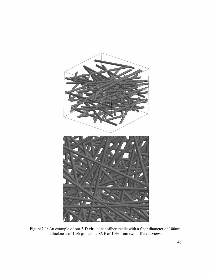
46

Figure 2.1: An example of our 3-D virtual nanofiber media with a fiber diameter of 100nm, a thickness of 1.96 µm, and a SVF of 10% from two different views.

47

Figure 2.2: Simulation domain and the boundary conditions

H

L

flow

Figure 2.3: Poiseuille flow in a 2-D duct

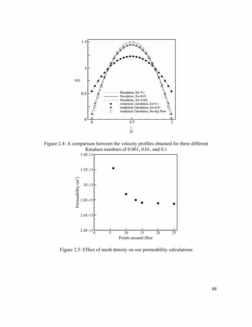
48

Figure 2.4: A comparison between the velocity profiles obtained for three different Knudsen numbers of 0.001, 0.01, and 0.1

Points around fiber

Perm

eabi

lity

(m2 )

0 5 10 15 20 252.4E-13

2.6E-13

2.8E-13

3E-13

3.2E-13

3.4E-13

Figure 2.5: Effect of mesh density on our permeability calculations

49

SVF

k/r2

0 0.02 0.04 0.06 0.08 0.1 0.120

1

2

3

4

5

6

7

8Jackson & James (1986)Modified Jackson & James (1986)Spielman & Goren (1968)Modified Spielman & Goren (1968)Current Simulation- No SlipCurrent Simulation- SlipOgorodnikov (1976)Fiber Diameter = 100 nm

a)

SVF

k/r2

0 0.02 0.04 0.06 0.08 0.1 0.120

1

2

3

4

5

6

7


c)

SVF

k/r2

0 0.02 0.04 0.06 0.08 0.1 0.120

1

2

3

4

5

6

7


d)

SVF

k/r2

0 0.02 0.04 0.06 0.08 0.1 0.120

1

2

3

4

5

6

7


b)

Figure 2.6: Our numerical simulations with and without slip velocity boundary condition are compared with the original and modified permeability expressions of Jackson and

James (1986) and Spielman and Goren (1968), as well as with the empirical correlation of Ogorodnikov (1976), for a fiber diameter of a) 100 nm, b) 400 nm, c) 700 nm, and d) 1000

nm

50

CHAPTER 3. 3-D Simulation of Particle Filtration in Electrospun Nanofibrous Filters♣


The adverse health effects and corresponding medical costs associated with particulate air

pollution are well-documented, and include increased risk of cancer, respiratory and

cardiovascular disease and decreased live expectancy. Fiber-based filters represent the

single largest mediator of particulate air pollution in commercial and residential

environments.

Recently, nanofiber filtration media have been produced by using a technique known as

electrospinning (the term “nanofiber” is often used in practice for fibers with a fiber

diameter smaller than about 500nm). It is well-documented that significant “slip” occurs

when a gas flows around a nanofiber (Brown 1993). This is because when the fiber

diameter is close to the mean free path of the gas molecules (e.g., 65nm for air in Normal

Temperatures and Pressures), flow field around the fiber can no longer be assumed to be in

a continuum regime, and the no-slip boundary condition at the fiber surface is invalid.

Because nanofibers can cause the so-called “slip effect”; they cause less resistance against

the air flow, leading to smaller pressure drop across the media. To the knowledge of the

♣ Content of this chapter is published in an article entitled “3-D Simulation of Particle Filtration in Electrospun Nanofibrous Filters” by Hosseini, S.A. and Tafreshi, H.V. in Powder Technology 201, 153-160 (2010b).

51

authors, there is no study in the literature devised to simulate the collection efficiency and

pressure drop of a nanofiber filter medium in realistic 3-D domains. As will be discussed

later in this paper, almost all existing models, starting with the work of (Kuwabara 1959),

are developed using oversimplified 2-D geometries wherein fibers are neatly placed in

square or hexagonal arrangements (e.g., Happel 1959, Stechkina and Fuchs 1965, Pich

1965 ,Pich 1966, Stechkina 1966, Lee and Liu 1982, Henry and Ariman 1983, Brown

1984, Rao and Faghri 1988, Liu and Rubow 1990, Payet 1991, Ramarao et al. 1994, Li and

Park 1997, Zhu et al. 2000, Brown 2001, Kirsh 2003). The predictions of such unrealistic

models were then corrected using variety of empirical coefficients, each valid for a given

range of fibers diameters, particle diameters, or flow hydrodynamic/thermal regimes. In a

previous work we simulated the performance of a fibrous filter medium using 3-D fibrous

geometries and with no empirical correction factors (Wang et al. 2006b). That work,

however, was limited to the case of microfiber media as the slip effect was not included in

the simulations. Moreover, particle capture via interception was neglected to ease the

calculations, which restricted our simulations to the filtration regimes with small particle-

to-fiber diameter ratios (i.e., particle diameters smaller than 500nm). In a recent work by

Maze et al. (2007), we simulated the deposition of nanoparticles on nanofiber media. In

this work, however, the air velocity field was assumed to be constant throughout the media

regardless of the presence of fibers, which can only be justified in the case of nanofibers

under reduced operating pressures, or elevated gas temperatures. In the current work, on

the other hand, there are no restrictions on the range of fiber diameters, particle diameters,

or hydrodynamic/thermal conditions of the gas. The simulation scheme presented here can

52

be used to model the collection efficiency and pressure drop of any fibrous media

challenged with any aerosol flows.

The next section presents our algorithm for generating virtual 3-D fibrous media. In

section 3.3, we describe the governing equations and the boundary conditions. In section

3.4, we describe the Lagrangian and Eulerian particle tracking methods together with our

C++ subroutines developed to enhance the capabilities of the CFD code from Fluent Inc.

Section 3.5 reports on our collection efficiency and pressure drop results obtained for

nanofibrous media, and it is followed by our conclusions presented in section 3.6.

3.2 – Virtual Nanofiber Media

To generate 3-D fibrous geometries resembling the microstructure of a fibrous medium, a

C++ computer program is developed to produce fibrous structures of different fiber

diameters, porosities, thicknesses, and orientations. The media generation process is based

on the µ -randomness algorithm and has been fully described elsewhere (Wang et al.

2006a, Maze et al. 2007). To mimic the microstructure of electrospun mats, we generated

fibrous structures with fibers positioned in horizontal planes and stacked on top of one

another to form a 3-D structure. Here, unlike our previous work, we allowed the fibers to

inter-penetrate, as this does not affect the pressure drop or collection efficiency of the

media, as long as the exact porosity is calculated correctly. The thickness of each layer is

considered to be an input parameter that can be used, among other parameters, to control

53

the SVF of the media, and was set to fd4.1 in the simulations reported here. Using polar

coordinates, and having the centerline equation of each fiber, the length of the fiber

confined in the simulation box is obtained to be used in estimating the SVF of each layer.

If the layer’s SVF is below the desired SVF, another fiber is added and the procedure is

repeated until it reaches the vicinity of the targeted value. The same process is repeated for

other layers until the desired thickness is achieved. Figure 3.1 shows an example of a 3-D

layered fibrous structure with a fiber diameter of 100 nm, a thickness of 1.96 µm and a

SVF of 7.5%. At the end of the generation process, the geometry is exported to Gambit

software (a preprocessor for Fluent code) via a script file. The exact SVF of the media is

calculated in Gambit and the structure is meshed for finite volume calculations conducted

via the Fluent code (see (Wang et al. 2006a, Wang et al. 2007) for more information on

meshing the fibrous structures).

3.3 – Flow Field Calculations

The air flow through our virtual fibrous media is assumed to be laminar and at steady state.

We have previously shown that for the range of fiber size and flow conditions considered

here (Reynolds number smaller than unity), there is a linear relationship between the flow

velocity and pressure drop, indicating that the inertial effects are negligible (Wang et al.

2007). The finite volume method (Patankar 1980) implemented in Fluent code is used to

solve the continuity and momentum equations in the absence of inertial effects:

0u v wx y z∂ ∂ ∂

+ + =∂ ∂ ∂

(3.1)

54

2 2 2

2 2 2

p u u ux x y z

µ⎛ ⎞∂ ∂ ∂ ∂

= + +⎜ ⎟∂ ∂ ∂ ∂⎝ ⎠ (3.2)

2 2 2

2 2 2

p v v vy x y z

µ⎛ ⎞∂ ∂ ∂ ∂

= + +⎜ ⎟∂ ∂ ∂ ∂⎝ ⎠ (3.3)

2 2 2

2 2 2

p w w wz x y z

µ⎛ ⎞∂ ∂ ∂ ∂

= + +⎜ ⎟∂ ∂ ∂ ∂⎝ ⎠ (3.4)


assumed to flow into the simulation domain through a velocity-inlet and leaves it from a

pressure-outlet boundary condition. Note that our uniform flow inlet and outlet boundary

conditions are placed far from the regions where strong velocity and/or pressure gradients

are expected. The inlet and outlet boundary conditions are placed at distance of fd20 , and

fd5 upstream and downstream of the media, respectively, where fd is the fiber diameter.

As it can be seen from Figure 3.2, we have used symmetry boundary conditions for the

sides of the computational box, even though there is no plane of symmetry in a disordered

medium. This is because if the in-plane size of the simulation domain is large, choice of

lateral boundary conditions will not affect the simulation results, as the flow is mainly in

the through-plane direction.

As the media generation process involves random processes, it is always necessary to

repeat each simulation a number of times and average the results. It is also important to

ensure that the domain size considered for the simulations is large enough so that the

results are not affected by any size-related artifact. Here, we used the Brinkman screening

55

length criterion which is given by k where k is the permeability of the medium being

simulated (Clague and Philips 1997, Clague et al. 2000). According to Clague and Phillips

(1997), a domain size about 14 times larger than the Brinkman’s length is sufficient to

smooth out statistical uncertainty of the results. The larger the domain size, the fewer the

number of repetitions that will be required. To obtain an estimate of the relevant domain

size to begin with, the expression of Davies (1973) has been used here.

Depending on the fiber diameter and the gas thermal conditions, continuum flow regime

( 310−<fKn ), slip-flow regime ( 25.010 3 <<−fKn ), transient regime ( 1025.0 << fKn ), or

free molecule regime ( 10>fKn ) can prevail inside a fibrous medium. Here ff dKn /2λ= is

the fiber Knudson number where )2/( 2 pdNTR maπλ = is the mean free path of gas

molecules. Air flow around most electrospun nanofibers is typically in the slip or transition

flow regimes. Slip velocity is permitted to occur at the fiber surface, as expected for flows

with non-zero Knudsen numbers. This has been done by defining the wall shear stress

using the Maxwell first order model (McNenly et al. 2005):

wv

vw n

uu∂∂−

= λσσ2 (3.5)

We have developed a C++ subroutine that works in Fluent environment and enables it to

handle the slip velocity at the fiber surface. To allow slip to occur, we modified the shear

stress at the wall using equation 3.5:

wv

vw u

σσ

λµτ

−=

2 (3.6)

56

Our virtual structures are meshed using tetrahedral elements, refined close to the fiber

surfaces. In an irregular structure, such as nonwoven media, there are regions where fiber-

to-fiber distance is very small, at the crossovers for instance, and regions where fibers are

relatively far from each other. The grid size required to mesh such a medium is often too

small. The computational grid used for Computational Fluid Dynamics (CFD) simulations

needs to be fine enough to resolve the flow field in the narrow gaps, and at the same time,

coarse enough to cover the whole domain without requiring infinite computational power.

To ensure that the results presented in this paper are independent of the number of grid

points considered for the simulations, we considered one of our fibrous structures and

meshed it with different mesh densities. This was done by adjusting the grid interval size

in such a way that it resulted in 6, 10, 13, 15, 20, and 25 grid points around the circular

cross-section of the fibers. The results of our mesh-independence study are presented in

Figure 3.3, where pressure drop is plotted versus the number of grid points around the

circular cross-section of the fibers. It can be seen that by increasing the mesh density,

pressure drop increases up to reach a plateau. In the simulations presented in this work, the

number of grid points on the circular cross-section of fibers was at least 15. The results

shown in Figure 3.3 are obtained for a medium with nmd f 400= , SVF=4.95%, and in the

absence of slip effect.

57

3.4 – Modeling Particle Capture in A Fibrous Medium

There are three basic mechanisms that lead to the capture of an aerosol particle in a neutral

filter medium. These are interception, inertial impaction, and Brownian diffusion.

Brownian diffusion is only important for small particles (about 200 nm or less).

Interception is important when the size of the particle and fiber are comparable, and

inertial impaction becomes considerable only when the particle’s momentum is not

negligible, either because of its large mass or high velocity. Note that van der Waals forces

are ignored in this study.

Here, we considered a convective-diffusive equation for the concentration of the small

particles based on the Eulerian approach (Friedlander 2000):

)( 2

2

2

2

2

2

zN

yN

xND

zNw

yNv

xNu

∂∂

+∂∂

+∂∂

=∂∂

+∂∂

+∂∂ (3.7)

To define equation 3.7 for the Fluent’s PDE solver, we developed a C++ subroutine that

was executed during the simulations. The diffusion coefficient in equation 3.7 is defined as

)3/( pc dTCD πµσ= in which )4.0257.1(1 /1.1 pKnpc eKnC −++= is the empirical factor of

Cunningham for slip correction at the surface of nanoparticles. It is assumed here that

particles that come in contact with the fibers will be captured and vanish from the domain.

Particle concentrations at the inlet and fiber surfaces are assumed to be 1=N and 0=N ,

respectively. At the outlet, we considered 0/ =∂∂ zN indicating that there is no change in

the nanoparticle concentration flux at the outlet (flow is in the z-direction).

58

Figure 3.4 is an example of our simulation results where the particle concentration contour

plots are shown in a plane slicing through a medium with a fiber diameter of 1000 nm and

an SVF of 7.5. In this figure, red to blue represent normalized particle concentration from 1

to zero (the blue color on the outlet plane is not part of the concentration contour plot and

is shown for better 3-D visualization only). Note that the particle concentration close to the

fibers is almost zero indicating particle deposition.

We also used the Lagrangian method, where each individual particle is tracked throughout

the solution domain, to calculate particle capture view interception and inertial impaction.

In the Lagrangian method, the force balance on a particle is integrated to obtain the particle

position in time. The dominant forces acting on a particle is the air drag force. For particle

Reynolds number smaller than unity, we have (Li and Ahmadi 1982):

( )2

18p

p

p p c

duu u

dt d Cµ

ρ= − (3.8)

( )pcpp

p vvCddt

dv−=

ρµ

218

(3.9)

( )pcpp

p wwCddt

dw−=

ρµ

218

(3.10)

where the subscript p denotes the particle properties. Particles in both Lagrangian and

Eulerian simulations were introduced to simulation domain from the inlet boundary

condition with uniform velocity and concentration profiles.

59

Standard Discrete Phase Model (DPM) in Fluent code treats the particles as point masses,

and therefore cannot calculate particle deposition due to interception. In this work, we

developed a C++ subroutine that modifies Fluent’s standard DPM module to include the

particle deposition via interception. This has been done by continuously monitoring the

distance between the particle’s center of mass and fibers’ surface during the trajectory

tracking in a loop. If a particle’s center of mass reaches a distance of one particle radius

from any fiber surface, our subroutine then eliminates it from the domain and considers it

as captured.

Figure 3.5 illustrates an example of the particle tracking exercise reported in this study. For

the sake of clarity, only a few particle trajectories are shown. For illustration purposes,

particles are released from 100 injection points located on the same plain as was shown in

Figure 3.4. To generate this figure, spherical objects are placed at the center of mass of

each particle as they travel through the medium. Size of the spherical symbols in the figure

is graphically chosen to be close to that of the actual particles (500nm) for illustration, i.e.,

the actual particle size is used only in the calculations, not in the graphical presentation. It

can be seen that our interception subroutine eliminates the trajectories that are intercepted

by fibers (see the magnified view of two intercepted trajectories in Figure 3.5b). Note that

particles do not interact with each other. Therefore, one can (and must) release a large

number of particles to correctly predict the particle capture.

60

3.5 – Results and Discussions

Kuwabara (1959) was the first to develop a mathematical theory (cell model) for predicting

the collection efficiency of fibrous filters in the continuum flow regime. Other researchers

later improved the work of Kuwabara by considering the so-called “fiber array” models

and obtained different expressions for pressure drop and particle collection efficiency of

fibrous media (see Spurny (1998) for a review). A filter’s pressure drop is a function of air

viscosity, filter thickness, face velocity, fiber diameter and material’s SVF, as:

2)(fdVf

hp µα=

∆ (3.10)

Here )(αf is a function of SVF only, and has different forms based on different theories.

The most popular correlation for calculating the pressure drop of a fibrous medium is the

empirical correlation of Davies (1973), given as:

)561(64)( 32/3 ααα +=Davf (3.11)

Our pressure drop per unit thickness results for fibrous media with fiber diameters ranging

from 100nm to 1000nm and different SVFs from 2.5% to 7.5% are shown in Figure 3.6. It

can be seen that pressure drop increases with increasing SVF, as expected. Predictions of

Davies equation are also added to this figure for comparison. It can be seen that Davies

correlation over-predicts the pressure drop of nanofiber media. This is because the media

used in Davies’ experiments comprised of fibers with a diameter ranging from 1.6µm to

80µm, and so his correlation is inaccurate in predicting the pressure drop of nanofiber

media where a significant slip takes place. Note that in our previous studies, we

61

demonstrated perfect agreement between the predictions of Davies correlation and our

CFD simulations conducted for microfiber media (Wang et al. 2006a, Jaganathan et al.

2008a, Jaganathan et al. 2008b, Tahir and Tafreshi, 2009).

In Figure 3.6, we have also included the predictions obtained via the empirical correlation

of Ogorodnikov (1976) obtained for slip and transition regime (Ogorodnikov 1976).

))1(15.1ln5.05.0(16)( 4αααα

−+−−=

fOgo kn

f (3.12)

It can be seen that very good agreement exists between our simulation results and the

empirical correlation of Ogorodnikov (1976), especially for fibers with very small

diameters. As the slip effect reduces for fibers with larger diameters (e.g., 1000nm),

Ogorodnikov (1976) loses its accuracy.

Efficiency of a filter medium can be obtained in terms of its thickness, SVF, and fiber

diameter if the total Single Fiber Efficiency (SFE), ∑E , is available. Efficiency of a fibrous

filter is given as (Hinds 1999):

))1(

4exp(1

απα

−−

−= ∑

fdtE

E (3.13)

The total SFE, ∑E , is the sum of SFEs due to interception, inertial impaction, and

Brownian diffusion (Hinds 1999). Inertial impaction for low-speed submicron particles is

quite negligible and will not be included in our discussion here. SFE is given as:

)1)(1(1 dR EEE −−−=∑ (3.14)

62

where RE and dE are single fiber efficiency due to interception a and Brownian diffusion,

respectively.

Different formulas are suggested for calculating the interception efficiency. Table 3.1

presents some commonly used SFE expression for particle capture due to interception. For

comparison purposes, we plotted efficiency of one of our virtual filter media due to

interception as predicted by these expressions in Figure 3.7. It can be observed that the

existing expressions do not perfectly agree with one another. This is simply because each

expression is empirically adjusted to for a given range of particles, fibers, and/or flow

regime, and so are not accurate for a wide range of parameters. Our particle capture results

due to interception are also shown in the figure for comparison.

There are also numerous different formulas suggested for calculating SFE due to diffusion.

Table 3.2 presents some commonly used SFE expressions for particle capture due to

Brownian diffusion. For comparison purposes, we plotted efficiency of one of our virtual

filter media due to Brownian diffusion as predicted by these expressions in Figure 3.8. It

again can be seen that the existing expressions do not perfectly agree with one another due

to their empirical nature. Our particle capture results due to Brownian diffusion are also

shown in the figure for comparison.

It is worth mentioning that unlike in a simulation, where particle capture via interception

can easily be decoupled from that due to Brownian diffusion, experimental data are always

63

the outcome of the combination of all the active collection mechanisms. It is therefore,

hard to find an empirical correction factor that is obtained purely based on interception or

diffusion data.

Figure 3.9 shows results of particle filtration simulation for media with different SVFs and

fiber diameters when challenged with particles having different diameters. We also added

the predictions of the expressions developed by (Liu and Rubow 1990) for diffusion and

interception to this figure. Note that the CFD results shown here are obtained by averaging

the results of similar simulations conducted for three statistically identical fibrous media. It

can be seen that, while the numerical values do not always perfectly match, our CFD

results are in close agreement with the predictions of the above semi-empirical

correlations. Note that unlike previous 2-D modeling studies in the literature (Lee and

Gieseke 1980), our modeling technique (and so the presented results) does not need any

empirical correction factors and is not limited to any special particle or fiber size range.

This modeling work builds a foundation for our future studies on particle loading and

filters lifecycle simulations.

It is known that a filter’s collection efficiency increases by increasing SVF or decreasing

fiber diameter. This, unfortunately, leads to an increase in the media’s pressure drop and

makes it difficult to judge whether or not the filter has been designed properly. To

circumvent this problem, Figure of Merit (also referred to as Quality Factor) is often used

in industry:

64

pPFOM

∆−=

)(ln (3.15)

Results of Figures 3.6 and 3.9 are used here to calculate the FOM of nanofiber media with

different SVFs and fiber diameters (see Figure 3.10). It can be seen that FOM increases by

decreasing the fiber diameter if the medium is challenged with particles generally larger

than about 500 nm. On the contrary, FOM decreases by decreasing the fiber diameter when

filter is exposed to particles with a diameter smaller than about 100 nm.

3.6 – Conclusions

Virtual 3-D geometries resembling the internal microstructure of electrospun fibrous

materials are generated in this work to simulate the pressure drop and collection efficiency

of nanofibrous media when challenged with aerosol particles. The numerical simulations

presented here are the most complete and realistic filter modeling published to date, and

unlike previous studies based on oversimplified 2-D geometries, do not need any empirical

correction factors. This modeling work strategy can be used to directly calculate the

pressure drop and collection efficiency of fibrous media with any fiber diameters when

challenged with aerosols of any particle sizes, and can be used study particle loading and

filters lifecycle simulations in future.

We, in particular, demonstrated that the existing empirical/semi-empirical correlations do

not agree with one another when deployed to predict collection efficiency of nanofiber

media. This is most probably due to the empirical nature of the correction factors used in

65

their development. Particle collection due to interception and Brownian diffusion, as well

as the slip effect at the surface of nanofibers, has been incorporated in our CFD

calculations by developing customized C++ subroutines that run in Fluent environment.

Our results show good general agreement with the existing correlations and can be used to

examine their accuracy. We also demonstrated that the popular correlation of Davies

(1973) fails to accurately predict the pressure drop of nanofiber media. Closer agreements

have been observed with the pressure drop correlation of Ogorodnikov (1976).

66

Figure 3.1: An example of our 3-D virtual media with a fiber diameter of 100nm, a thickness of 1.96 µm, and an SVF of 7.5%.

67

Figure 3.2: Simulation domain and boundary conditions are shown. Red spheres are placed at the inlet to visualize the position at which the particles are injected. For the clarity of the

illustration only a few number of particles are shown.

68

Points around fiber

Pres

sure

drop

(Pa)

0 5 10 15 20 2542

44

46

48

50

52

Figure 3.3: Pressure drop as a function of mesh density around the circular perimeter of fiber. The results are obtained for a medium with a fiber diameter of 400 nm and an SVF

of 4.95%.

Figure 3.4: An example of our particle concentration contour plots with nmd p 50= shown in a plain slicing through a medium with a fiber diameter of 1000nm and an SVF of 7.5%.

Red to blue represents normalized particle concentration from 1 to 0.

69

b)

a)

Figure 3.5: a) an example of our particle trajectory tracking with nmd p 500= shown in a plain slicing through a medium with a fiber diameter of 1000nm and an SVF of 7.5%, b) magnified view of particle trajectory termination at a distance of 2/pd from the fibers.

Note that the spherical symbols in the figure do not represent the actual particle size and are chosen for illustration only.

70

SVF

dp/t

(pa/

m)

2 4 6 8104

105

106

107

108

df = 100 nmdf = 200 nmdf = 300 nmdf = 400 nmdf = 700 nmdf = 1000 nm

Figure 3.6: Pressure drop per unit thickness of different media with different SVFs and

fiber diameters are compared with the predictions of Davies (black lines) and Ogorodnikov (red line) empirical correlations. Dashed-dotted line (-⋅-), long-dashed line (− −), solid line (⎯), dotted line (⋅⋅⋅), dashed line (- -), and dashed-double-dotted line (-⋅⋅-), represent fiber

diameters of 1000 to 100 nanometers, respectively.

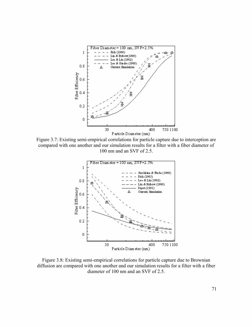
71

Figure 3.7: Existing semi-empirical correlations for particle capture due to interception are compared with one another and our simulation results for a filter with a fiber diameter of

100 nm and an SVF of 2.5.

Figure 3.8: Existing semi-empirical correlations for particle capture due to Brownian diffusion are compared with one another and our simulation results for a filter with a fiber

diameter of 100 nm and an SVF of 2.5.

72

Figure 3.9: Total filter efficiency is calculated by adding our simulation results for particle

capture via Brownian diffusion and direct interception, and are compared with the predictions of the expressions given by Liu and Rubow (1990), as an example. Note that

the SVFs of the results presented in this figure are approximate values with a 10% margin of error from the stated values in the legend (i.e., 2.5%, 5.0%, and 7.5%).

73

Figure 3.10: Figure of merit is versus particle diameter for a) media with an SVF of 5.0% but different fiber diameters, and b) media with a fiber diameter of 300nm but different

SVFs.

74

Investigator(s) SFE expressions for interception

Lee and Gieske (1980)

Pich (1966)

Liu and Rubow (1990)

Lee and Liu (1982)

)ln5.0(996.1)ln5.075.0(2)1ln()1)(996.11(2)1()1( 1

αα −−+−−+++++−+

=−

KnRRKnRRER

rR CR

RKu

E)1(

16.02

+⎟⎠⎞

⎜⎝⎛ −

=α

)1(16.0

2

RR

KuER +

−=

α

Rkn

C fr

996.11+=

))1(3/(2,)1(

1 2

αα−=

+−

= mR

RKu

E mR

Table 3.1: Some of the existing single fiber efficacy expressions for particle capture due to interception.

Investigator(s) SFE expressions for diffusion

Stechkina (1966)


Payet (1991)

Lee and Liu (1982)

Pich (1965)

1323/1 62.09.2 −−− += PePeKuED

323/116.1 −⎟

⎠⎞

⎜⎝⎛ −

= PeKu

EDα

dD CPeKu

E 323/116.1 −⎟

⎠⎞

⎜⎝⎛ −

=α 3

1

))1((388.01Ku

PeKnC fdα−

+=

'323/116.1 ddD CCPe

KuE −⎟

⎠⎞

⎜⎝⎛ −

=α

]12[&)(11

RubowLiuDd E

C+

=′

)62.01(27.2 3/13/1323/1 −−− += KuKnPePeKuED


Brownian diffusion.

75

CHAPTER 4. Modeling Particle Filtration in Disordered 2-D Domains: A Comparison with Cell Models♣


Fibrous filters are the single largest mediator of particulate air pollution in commercial and

residential environments. For the past fifty years, scientists around the globe have been

trying to develop mathematical formulations to predict the performance of fibrous filters

and improve their effectiveness. Starting with the work of Kuwabara (1959), existing

analytical/numerical studies that built the foundation of current filtration theory were

formulated using 2-D solution domains in which the fibers were arranged in either square

or staggered (i.e., ordered) positions (e.g., Lee and Gieseke 1980, Pich 1965, Pich 1966,

Liu and Rubow 1990, Lee and Liu 1982, Stechkina 1966, Payet 1991, Hinds 1999, Spurny

1998, Brown 1993, Henry et al. 1983, Rao and Faghri 1988, Li and Park 1997, Ramarao et

al. 1994, Brown 1984,Zhu et al. 2000, Kirsh 2003, Wang and Pui 2009, Jaganathan et al.

2008a, Fotovati et al. 2010). The air and particle flow field were then calculated in a unit

cell of such periodic geometries to find analytical expressions for the pressure drop and

particle capture efficiency of real fibrous filter media (in which fibers are randomly

distributed in 3-D space). Treating a filter medium as an ordered array of fibers in 2-D

♣Content of this chapter is published in an article entitled “Modeling Particle Filtration in Disordered 2-D Domains: A Comparison with Cell Models”, by Hosseini, S.A. and Tafreshi, H.V., in Separation and Purification Technology 74, 160-169 (2010c).

76

domains may help in obtaining rough estimations of the pressure drop and collection

efficiency of real filter media, but such expressions often need empirical correction factors

(each valid for a given range of fiber diameters, particle diameters, or flow

hydrodynamic/thermal regimes) to improve their accuracy. We have previously

demonstrated the advantages of generating virtual 3-D models that mimic the internal

microstructure of fibrous media for simulating the pressure drop and collection efficiency

(Wang et al. 2006b, Maze et al. 2007, Wang et al. 2007, Jaganathan et al. 2008c, Tahir and

Tafreshi 2009, Tafreshi et al. 2009, Hosseini and Tafreshi 2010a). Such 3-D models do not

necessarily need empirical correction factors, and their predictions can directly be used for

product design and development. The problem with 3-D models, however, is that they

require excessive computational power, which may prohibit extensive parameter studies,

especially in the presence of particle loading. In the current paper, we simulate the pressure

drop and particle collection efficiency of fibrous media in large, but 2-D, simulation

domains comprised of randomly distributed fibers. Our main objective in this paper is to

examine whether or not the simulations conducted in disordered 2-D fibrous geometries

can generate predictions comparable to those of 3-D simulations (or those obtained using

the semi-analytical correlations from the literature). We also investigate the influence of

aerodynamic slip on particle collection efficiency and pressure drop, and compare them

with the existing correlations in the literature.

77

In the next section, we first describe our algorithm for generating disordered 2-D

simulation domains comprised of randomly distributed fibers. We then discuss our

governing equations and their boundary conditions. In section 4.3, we present our particle

tracking methods and explain the subroutines that we developed to enhance performance of

Fluent CFD code. Our results and discussion are given in section 4.4, and they are

followed by our conclusions outlined in section 4.5.

4.2 – Flow Field

To generate 2-D random fibrous geometries, a C++ computer program is developed to

produce fibrous structures of different porosities. The media generation process is

explained in the flow chart shown in Figure 4.1. Fibers are treated as circles randomly

placed in a square domain. The media generation starts by sequentially adding the fibers

into a square domain with a given size. Distance between a new fiber and the existing ones

are continuously monitored to avoid fiber-fiber overlaps. Moreover, to ensure that a high-

quality mesh can be generated inside the domain, fibers were not permitted to touch one

another. To do this, a minimum gap of fd1.1 was enforced between the fibers’ center-to-

center distance (df is the fiber diameter). To generate periodic boundary conditions on the

lateral sides of the domain, any fiber touching the lower or upper boundaries were shifted

in the y-direction by a distance equal to the size of the simulation box. This procedure

continues until a desired porosity is reached. At the end of the media generation process,

the geometry is exported to Gambit software (a preprocessor for Fluent CFD code) via a

78

script file for meshing. The mesh files were then exported to Fluent for finite volume

calculations. Figure 4.2 shows an example of our 2-D random fibrous geometry with a

fiber diameter of 10 µm, a thickness of 400 µm, and a porosity of 85%.

Stokes flow is assumed to prevail in the filter media. We therefore solved the momentum

equations in the absence of inertial effects:

0=∂∂

+∂∂

yv

xu (4.1)

⎟⎟⎠

⎞⎜⎜⎝

⎛

∂∂

+∂∂

=∂∂

2

2

2

2

yu

xu

xp µ (4.2)

⎟⎟⎠

⎞⎜⎜⎝

⎛

∂∂

+∂∂

=∂∂

2

2

2

2

yv

xv

yp µ (4.3)


assumed to flow into the simulation domain through a velocity-inlet, and leaves it from a

pressure-outlet boundary condition. Note that our uniform flow inlet and outlet boundary

conditions are placed far from the regions where strong velocity and/or pressure gradients

are expected. The inlet and outlet boundary conditions are placed at a distance of

fd20 (upstream) and fd5 (downstream) of the media. As it can be seen from Figure 4.2, we

have used periodic boundary conditions for the sides of the computational box.

Nevertheless, choice of the lateral boundary conditions does not affect the simulation

results as the flow is mainly in the through-plane direction.

79

Our solution domains are meshed using uniformly distributed triangular elements (no

refining or coarsening). To ensure that our results are mesh-independent, we considered

one of our fibrous structures and meshed it with different number of cells. This was done

by adjusting the grid interval size in such a way that it resulted in 10 to 100 grid points

around the fibers. The results of our mesh independence study are presented in Figure 4.3,

where pressure drop per thickness is plotted versus the number of grid points on a fiber

perimeter. It can be seen that by increasing the mesh density, pressure drop increases to

reach a plateau. In the simulations presented in this work, the number of grid points on a

fiber perimeter was set to 50.

As the fibers are randomly distributed in the simulation domain, it is always necessary to

repeat each simulation a number of times, and average the results. It is also important to

ensure that the domain size considered for the simulations is large enough so that the

results are not affected by any size-related artifact. The larger the domain size, the fewer

the number of required repetitions. To ensure that the size of the simulation domain is

large enough, we studied the influence of number of fibers on the pressure drop per unit

thickness of the media, as shown in Figure 4.4. It can be seen that at a porosity of 85%,

pressure drop per unit thickness is independent of the domain size, if number of fibers is

more than about 300. We used 300 fibers in the simulations reported in this paper. Note

that statistical uncertainty of the results normally increases as porosity increases. We

therefore, increased the number of repetitions when the porosity was higher than 85%.

80

4.3 – Particle Flow and Capture


filter medium. These are interception, inertial impaction, and Brownian diffusion. Here, we

considered a convective-diffusive equation for the concentration of the small particles

(smaller than 500nm) based on the Eulerian approach, and in the absence of any external

forces (Friedlandar 2000):

)( 2

2

2

2

yN

xND

yNv

xNu

∂∂

+∂∂

=∂∂

+∂∂ (4.4)

To define equation 4.4 for the Fluent’s PDE solver, we developed a C++ subroutine that

was executed during the simulations. The diffusion coefficient in equation 4.4 is defined as

)3/( pc dTCD πµσ= in which )4.0257.1(1 /1.1 pKnpc eKnC −++= is the empirical factor of

Cunningham for slip correction at the surface of nanoparticles (Hinds 1999). It is assumed

here that particles that come in contact with the fibers will be captured, and vanish from

the domain. Particle concentrations at the inlet and fiber surfaces are assumed to be 1=N

and 0=N , respectively. At the outlet, we considered 0/ =∂∂ xN indicating that there is no

change in the nanoparticle concentration flux at the outlet.

Figure 4.5 is an example of our simulation results, where the particle concentration contour

plots are shown in a medium with a porosity of 85%. In this figure, red to blue represent

normalized particle concentration from 1 to zero. Note that the particle concentration close

81

to the fibers is almost zero, indicating that the particles are deposited and their

concentration is almost zero.

We also used the Lagrangian method, where each particle is individually tracked

throughout the solution domain, to calculate particle capture via interception and inertial

impaction. In the Lagrangian method, the force balance on a particle is integrated to obtain

the particle position in time. The dominant forces acting on a particle are the air drag force

and the Brownian forces. For particle Reynolds number smaller than unity, we have

(Friedlander 2000):

( ) )(182 tnuu

Cddtdu

ipcpp

p +−=ρµ (4.5)

( ) )(182 tnvv

Cddtdv

jpcpp

p +−=ρµ (4.6)

where the subscript p denotes properties associated with the particle. The first term on the

right hand side of this equation is the drag term, whereas the second term, )(tni , is the

Brownian force per unit mass defined as (Li and Ahmadi, 1992):

tSGtn ii ∆

= 0)( π (4.7)

where 0S is the corresponding spectral intensity of the noise given by (Li and Ahmadi,

1992):

cpp CSdkTS

2520216ρπ

ν= (4.8)

82

and iG is a random number chosen from a normal distribution with a zero mean and a unit

variance. Particles in both Lagrangian and Eulerian simulations were introduced to the

simulation domain from the inlet boundary condition with uniform velocity and

concentration profiles.

The standard Discrete Phase Model (DPM) implemented in Fluent code treats the particles

as point masses, and therefore can only calculate particle deposition due to inertial

impaction (but not interception). In this work, we developed a C++ subroutine that

modifies Fluent’s standard DPM module to include the particle deposition via interception.

This has been done by continuously monitoring the distance between the particle’s center

of mass and fibers’ surface during the trajectory tracking in a loop. If a particle’s center of

mass reaches a distance of one particle radius from any fiber surface, our subroutine then

eliminates it from the domain, and assume it is captured. The Fluent’s DPM also fails to

correctly predict the particle trajectories when the Brownian motion is not negligible. We

therefore, developed another subroutine to redefine equations 4.7 and 4.8 for Fluent. To

ensure that our Brownian diffusion subroutine has been correctly implemented in Fluent,

we considered a square simulation domain with no air velocity (figure not shown for the

sake of brevity). Series of particles with given diameters were injected in the middle of the

square domain and their mean square displacement were calculated. Figure 4.6 shows an

example of such calculations. According to the Einstein equation, one half of the slope of

83

this curve is expected to be the particle diffusion

coefficient, ( ) ( )2t

2

t(0))(

21lim(0))(

21lim yty

txtx

tD −=−=

→∞→∞.

Figure 4.7a and b show examples of the particle trajectory calculations with and without

Brownian diffusion. For illustration purposes, particles are released from a limited number

of injection points. It can be seen that our interception subroutine eliminates the trajectories

that are intercepted by fibers. Note that particles do not interact with each other. Therefore,

one can (and must) release a large number of particles to correctly predict the particle

capture. To further investigate the influence of number of injections on the particle capture

predictions, we released different numbers of particles at the inlet, and studied the

interception efficiency of a given medium. To increase the number of injections at the

inlet, one needs to increase the number of cells at the inlet. Since we used uniform mesh

distribution (no mesh stretching), increasing the number of grid points on a fiber’s

perimeter results in an increase in the number cells at the inlet. Figure 4.8a presents the

effect of mesh density (number of injection at the inlet) on the interception capture

efficiency. It can be seen that for the mesh density considered in this work (50 mesh count

per fiber), the number of particle injections has no influence on the outcomes of our

Lagrangian particle capture predictions. We also studied the effect of mesh density on the

diffusion capture efficiency conducted via the Eulerian approach. It can be seen that the

diffusion capture is less sensitive to the mesh density (see Figure 4.8b).

84


Kuwabara (1959) was the first to develop a mathematical theory (cell model) for predicting

collection efficiency of fibrous filters. Other researchers later improved the work of

Kuwabara by considering the so-called “fiber array” models, and obtained different

expressions for pressure drop and particle collection efficiency of fibrous media (see

Spurny 1998, and Brown 1993 for a review). A filter’s pressure drop depends on the air

viscosity, filter thickness, flow face velocity (here 0.1m/s unless otherwise stated), fiber

diameter, and fibers volume fraction, as:

2)(f

d dVf

tp µα=

∆ (4.9)

where dimensionless pressure drop, )(αdf , is only a function of fibers volume fraction,

and has different forms based on different theories. For the Kuwabara’s cell model, )(αdf

is given as:

Kufd

αα 16)( = (4.10)

in which 44

32

ln 2ααα−+−−=Ku is the Kuwabara’s hydrodynamic coefficient (Kuwabara

1959). Our pressure drop per unit thickness results for fibrous media with different

porosity from 80% to 95% are shown in Figure 4.9. It can be seen that pressure drop

increases with increasing fibers’ volume fraction, as expected. Predictions of the

expression derived by Kuwabara (1959) and that proposed by Drummond and Tahir

(1984), 12 )774.12476.1ln(32)( −−+−−= αααααdf , are also added to this figure for

85

comparison. Note that these two expressions are derived for ordered 2-D fibrous

geometries. We have previously shown that ordered 2-D geometries tend to over-predict

the pressure drop of a real (i.e., 3-D) fibrous geometry (see (Tahir and Tafreshi 2009) and

references there). Disordered 2-D fibrous geometries, however, tend to result in pressure

drop values somewhere between those of ordered 2-D and disordered 3-D media. This has

been shown here by adding the well known empirical equation of Davies (1973),

)561(64)( 32/3 ααα +=df , and Jackson and James (1986), ])931.0)ln([3/(80)( −−= αααdf , to

Figure 4.9a.

To investigate the effects of aerodynamic slip on the pressure drop, we simulated a series

of media having a fiber diameter of 100 nm but different fibers volume fractions (see

Figure 4.9b). We also calculated pressure drop of these media without including the

aerodynamic slip in the calculations, for comparison purposes only. It can be seen that

aerodynamic slip significantly reduces the pressure drop of a filter medium. As explained

in a previous work (Hosseini and Tafreshi 2010a), none of the existing empirical or

analytical expressions in the literature are accurate in predicting the pressure drop of

fibrous medium in the slip flow regime. The only available empirical correlation is the

work of Ogorodnikov (1976), ))1(15.1ln5.05.0/(16)( 4αααα −+−−= fd knf , which is

obtained for media with a fiber diameter in the range of 200 nm. As expected, simulation

results obtained from disordered 2-D fibrous domains are again higher than those of 3-D

fibrous geometries (e.g., real media) (see Hosseini and Tafreshi 2010a).

86

Efficiency of a filter medium can be obtained in terms of its thickness, fibers volume

fraction, and fiber diameter if the total Single Fiber Efficiency (SFE), ∑E , is available.

Efficiency of a fibrous filter is given as (Brown 1993):

))1(

4exp(1

απα

−−

−= ∑

fdtE

E (4.11)

The total SFE, ∑E , is the sum of SFEs due to interception, inertial impaction, and

Brownian diffusion (Spurny 1998, Brown 1993). Inertial impaction for low-speed

submicron particles is relatively small and often negligible. The total SFE is given as

(Brown 1993):

)1)(1(1 dR EEE −−−=∑ (4.12)

where RE and dE are single fiber efficiency due to interception a and Brownian diffusion,

respectively. Different formulas are suggested for calculating the interception (Table 4.1)

and diffusion (Table 4.2) efficiencies. In Figure 4.10 and 4.11, we compare the single fiber

efficiency obtained from our simulations with those given in these tables. The horizontal

axis in these figures is Peclet number, defined as DVdPe f /= . Results shown in these two

figures are obtained for different fibrous media having a fiber diameter of 10µm (slip

effect not included). It can be seen that there is good agreement between the predictions of

our disordered media and those of the existing semi-analytical models. Note that the CFD

results shown here are obtained by averaging the results of similar simulations conducted

for several statistically identical fibrous media. Note also that we have removed the

87

contribution of inertial impaction (even though quite small) from the Lagrangian particle

tracking results shown in Figure 4.11.

To further explore the accuracy of our modeling work and compare it with the existing

semi-analytical expressions, we simulated filters with different fiber diameters ranging

from 100 to 1000 nanometers. For such small fiber diameters, significant slip is expected

to occur on the fibers’ surface. We therefore developed another subroutine to define the

wall shear stress for the Fluent code, using the Maxwell first order model (see Hosseini

and Tafreshi 2010a, for more information):

nuu

v

vw ∂

∂−= λ

σσ2 (4.13)

In Figure 4.12 and 4.13, we present the single fiber efficiency due to Brownian diffusion

and interception, respectively, for media with a porosity of 95% but different fiber

diameters. The results are presented with and without the slip effect. It can be seen that

aerodynamic slip tends to improve the collection efficiency of a fibrous medium. It can

again be seen that there is good agreement between the predictions of our disordered media

and those of the existing semi-analytical models. In Figure 4.12, we also compared our

single fiber efficiencies obtained via both Lagrangian and Eulerian methods. Good

agreement between these values validates our implementation of these methods in Fluent

code.

88

Here, we also compare our results obtained from disordered 2-D filter simulations with

those we previously reported using their more sophisticated (and computationally more

demanding) 3-D fibrous geometries (see Figure 4.14) (Friedlander, 2000). It can be seen

that disordered 2-D models tend to slightly under-predict a filter’s collection efficiency at

low Peclet numbers, but slightly over-predict them at high Peclet values.

From Figures 4.9 to 4.14, one can conclude that both disordered 2-D and disordered 3-D

filter models seem to have good agreement with the predictions of the existing empirically-

modified cell or array models in literature. This is an important conclusion, as it indicates

that one may be able to estimate the pressure drop and collection efficiency of a fibrous

filter purely computationally, which is, of course, more economical.

For the completeness of the study, here we also add a series of simulations in which

inertial impaction is not negligible. In these simulations, the fiber diameter and volume

fraction are kept constant at 1µm and 5%, respectively. The air face velocity and particle

diameters, however, are changed to obtain a range of Stk numbers between almost 0 and 5

( fcpp dVCdStk ηρ 18/2= ). Our simulation results are compared with three different

expressions obtained for low, moderate, and high values of Stokes numbers from the book

of Brown (see Table 4.3) (Brown 1993).

89

4.5 – Conclusions

Existing semi-analytical aerosol collection efficiency expressions that have been developed

over the past fifty years are based on modeling the disordered 3-D structure of a fibrous

filter by 2-D periodic geometries in which the fibers are packed in square or staggered

configurations. In this paper, we use disordered 2-D fibrous geometries for pressure drop

and collection efficiency calculation in both slip and no-slip flow regimes (i.e., micro- and

nanofiber media). Particle collection due to interception and Brownian diffusion

(Lagrangian and Eulerian methods) as well as the aerodynamic slip boundary condition on

the fibers surface have been included in our CFD calculations by developing customized

C++ subroutines that run in Fluent environment. The results of our simulations are

compared with those of the previously developed ordered 2-D semi-analytical models, and

our previous 3-D simulations, to report reasonably good agreement. Our results indicate

that cost-effective 2-D simulations conducted in domains comprised of disordered fiber

arrangement can be considered for obtaining good estimates of the collection efficiency

and pressure drop of fibrous filters.

Our simulations of fibrous filters operating at filtration regimes with considerable inertial

impaction revealed reasonable agreement with the existing expressions that have been

developed over the past decades.

90

create a random position for the center of a new fiber

move the fiber down (or up)

by one box height

fiber touching the upper (or lower)

boundary

check for overlaps

add the fiber to the domain and update the SVF

reachedThe desired

SVF

Finish

Figure 4.1: Flow chart of our disordered 2-D media generation algorithm.

91

Vel

ocity

Inle

t

Periodic

Periodic

Pressure OutletV

eloc

ity In

let

Periodic

Periodic

Pressure Outlet

20df 5df

Vel

ocity

Inle

t

Periodic

Periodic

Pressure OutletV

eloc

ity In

let

Periodic

Periodic

Pressure OutletV

eloc

ity In

let

Periodic

Periodic

Pressure OutletV

eloc

ity In

let

Periodic

Periodic

Pressure Outlet

20df 5df

Figure 4.2: An example of the simulation domains used for the simulations reported in this work together with the boundary conditions.

92

Number of Meshes per Fiber

Pres

sure

Dro

ppe

rThi

ckne

ss(P

a/m

)

0 20 40 60 80 100

85000

90000

95000

100000

105000

110000

115000SVF = 15%

Figure 4.3: Influence of mesh density on pressure drop calculations. The results are obtained for a medium with a fiber diameter of 10µm and a volume fraction of 15%.

Number of Fibers in Domain

Pres

sure

Dro

ppe

rThi

ckne

ss(p

a/m

)

0 200 400 600

80000

100000

120000

140000 SVF = 15%

Figure 4.4: Influence of the domain size (number of fibers) on pressure drop calculations. The results are obtained for a medium with a fiber diameter of 10µm and a volume fraction

of 15%.

93

Figure 4.5: An example of our particle concentration contour plots with nmd p 50= shown for a medium with a fiber diameter of 10µm and a volume fraction of 15%. Red to blue

represents normalized particle concentration from 1 to 0.

Time (s)

<x

2>

0 1E-05 2E-05 3E-05 4E-050

1E-14

2E-14

3E-14

4E-14

5E-14

6E-14

< x 2 > = 2Dtd p = 100 nm

Figure 4.6: Mean square displacement calculated for an ensemble of particles having a diameter of 100 nm suspended in quiescent air.

94

a)

b)

Figure 4.7: An example of our particle trajectory tracking with 50=pd nm shown for a medium with a fiber diameter of 100 nm and a fiber volume fraction of 5%. Trajectories

are shown with (b) and without (a) the Brownian diffusion.

95

dp (nm)

Inte

rcep

tion

Effic

ienc

y

0 500 10000

0.1

0.2

0.3

0.4

0.5 Mesh Count per Fiber = 20Mesh Count per Fiber = 25Mesh Count per Fiber = 30Mesh Count per Fiber = 50Mesh Count per Fiber = 75

dp (nm)

Diff

usio

nEf

ficie

ncy

0 100 200 300 400 5000

0.1

0.2

0.3

0.4

0.5

0.6

0.7

Mesh Count per Fiber = 20Mesh Count per Fiber = 25Mesh Count per Fiber = 30Mesh Count per Fiber = 50Mesh Count per Fiber = 75

a)

b)

Figure 4.8: Influence of number of grid points around the perimeter of a fiber on collection efficiency due to interception (a) and diffusion (b). The results are obtained for a fibrous

medium with a fiber diameter of 10µm and a fibers volume fraction of 15%.

96

df=100nm

Fiber Volume Fraction

fd

5 10 15 20

2

4

6

8

10

12

14Kuwabara (1959)Drummond & Tahir (1984)Davis (1973)Jackson & James (1986)Ogorodnikov (1976)No Slip BCSlip BC

df=10µm

Fiber Volume Fraction

fd

5 10 15 20

2

4

6

8

10

12

14Kuwabara (1959)Drummond & Tahir (1984)Davis (1973)Jackson & James (1986)No Slip BC

Figure 4.9: Dimensionless pressure drop, )(αpf , calculated for fibrous media having fiber diameters of 10µm (a) and 100 nm (b) at different volume fractions of 5, 10, 15, and 20

percent. Predictions of the cell model of Kuwabara (1959), fiber array model of Drummond and Tahir (1984), empirical correlations of Davies (1973), and Ogorodnikov

(1976), as well as the analytical expression of Jackson and James (1986) are also added for comparison. A comparison is also made between the simulation results obtained with and

without the aerodynamic slip for the case shown in (b).

97

Pe

Sing

leFi

berE

ffic

ienc

y

102 103 104

0

0.02

0.04

0.06

0.08

0.1

0.12 Current SimulationStechkina (1966)Liu and Rubow (1990)Payet (1991)Lee and Liu (1982)Pich (1965)

SVF = 5%

PeSi

ngle

Fibe

rEff

icie

ncy

102 103 104

0

0.02

0.04

0.06

0.08

0.1

0.12

0.14

Current SimulationStechkina (1966)Liu and Rubow (1990)Payet (1991)Lee and Liu (1982)Pich (1965)

SVF = 10%

Pe

Sing

leFi

berE

ffic

ienc

y

102 103 1040

0.02

0.04

0.06

0.08

0.1

0.12


SVF = 15%

Pe

Sing

leFi

berE

ffic

ienc

y

102 103 1040

0.02

0.04

0.06

0.08

0.1

0.12

0.14

0.16


SVF = 20%

Figure 4.10: Diffusion Single Fiber Efficiency obtained from our CFD simulations are compared with the predictions of existing semi-analytical correlations for media with a


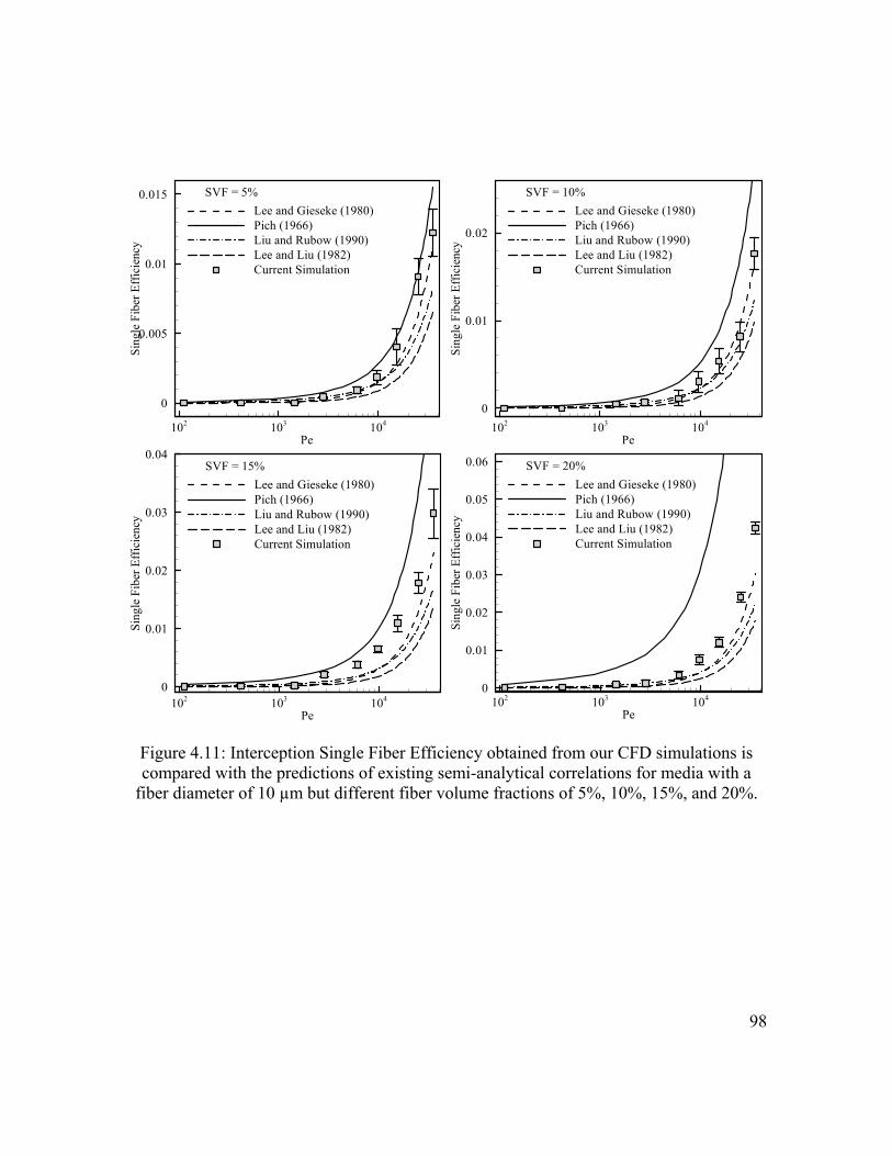
98

Pe

Sing

leFi

berE

ffic

ienc

y

102 103 104

0

0.005

0.01

0.015Lee and Gieseke (1980)Pich (1966)Liu and Rubow (1990)Lee and Liu (1982)Current Simulation

SVF = 5%

PeSi

ngle

Fibe

rEff

icie

ncy

102 103 104

0

0.01

0.02

Lee and Gieseke (1980)Pich (1966)Liu and Rubow (1990)Lee and Liu (1982)Current Simulation

SVF = 10%

Pe

Sing

leFi

berE

ffic

ienc

y

102 103 1040

0.01

0.02

0.03

0.04


SVF = 15%

Pe

Sing

leFi

berE

ffic

ienc

y

102 103 1040

0.01

0.02

0.03

0.04

0.05

0.06


SVF = 20%

Figure 4.11: Interception Single Fiber Efficiency obtained from our CFD simulations is compared with the predictions of existing semi-analytical correlations for media with a


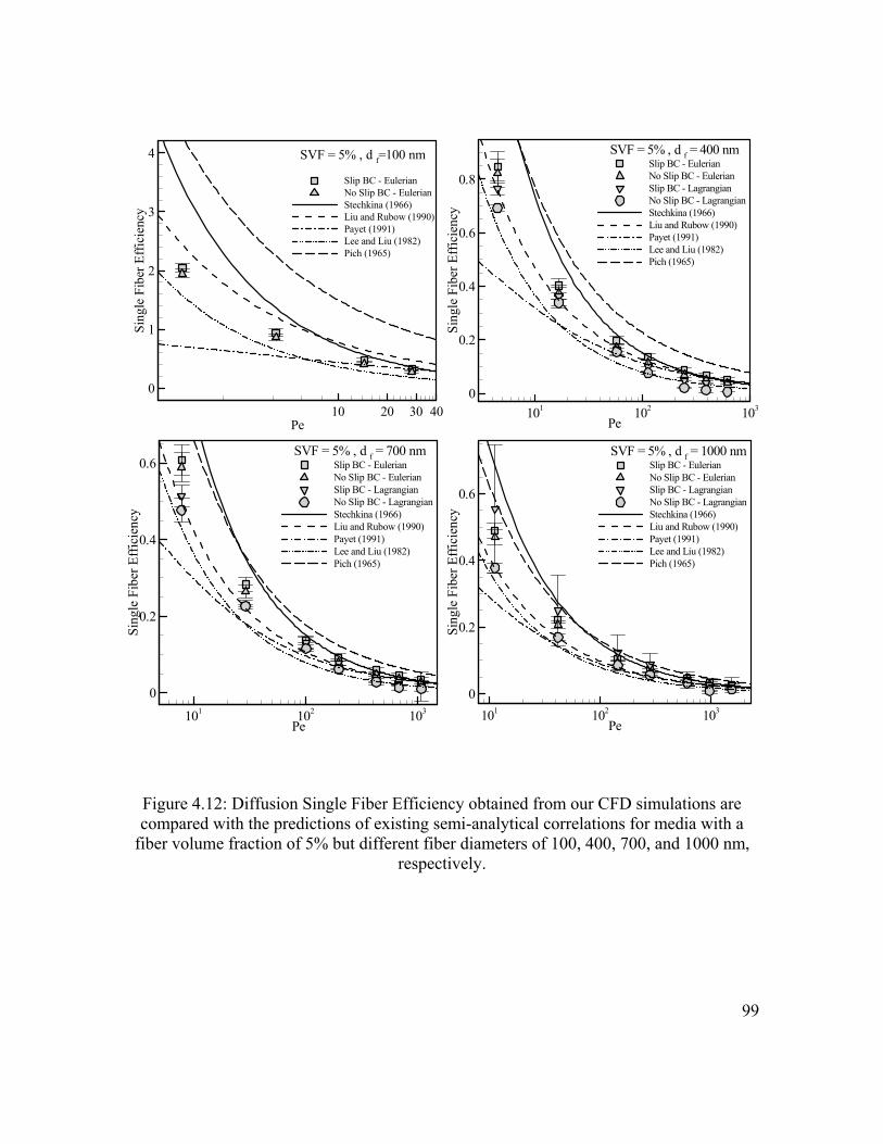
99

Pe

Sing

leFi

berE

ffic

ienc

y

10 20 30 40

0

1

2

3

4

Slip BC - EulerianNo Slip BC - EulerianStechkina (1966)Liu and Rubow (1990)Payet (1991)Lee and Liu (1982)Pich (1965)

SVF = 5% , d f=100 nm

Pe

Sing

leFi

berE

ffic

ienc

y

101 102 1030

0.2

0.4

0.6

0.8Slip BC - EulerianNo Slip BC - EulerianSlip BC - LagrangianNo Slip BC - LagrangianStechkina (1966)Liu and Rubow (1990)Payet (1991)Lee and Liu (1982)Pich (1965)

SVF = 5% , d f = 400 nm

Pe

Sing

leFi

berE

ffic

ienc

y

101 102 103

0

0.2

0.4

0.6 Slip BC - EulerianNo Slip BC - EulerianSlip BC - LagrangianNo Slip BC - LagrangianStechkina (1966)Liu and Rubow (1990)Payet (1991)Lee and Liu (1982)Pich (1965)

SVF = 5% , d f = 700 nm

Pe

Sing

leFi

berE

ffic

ienc

y

101 102 103

0

0.2

0.4

0.6

Slip BC - EulerianNo Slip BC - EulerianSlip BC - LagrangianNo Slip BC - LagrangianStechkina (1966)Liu and Rubow (1990)Payet (1991)Lee and Liu (1982)Pich (1965)

SVF = 5% , d f = 1000 nm

Figure 4.12: Diffusion Single Fiber Efficiency obtained from our CFD simulations are compared with the predictions of existing semi-analytical correlations for media with a

fiber volume fraction of 5% but different fiber diameters of 100, 400, 700, and 1000 nm, respectively.

100

Pe

Sing

leFi

berE

ffic

ienc

y

10 20 30 400

1

2Slip BCNo slip BCLee and Gieseke (1980)Pich (1966)Liu and Rubow (1990)Lee and Liu (1982)

SVF = 5% , d f = 100 nm

PeSi

ngle

Fibe

rEff

icie

ncy

101 102 1030

0.2

0.4

0.6

0.8

1Slip BCNo slip BCLee and Gieseke (1980)Pich (1966)Liu and Rubow (1990)Lee and Liu (1982)

SVF = 5% , d f = 400 nm

Pe

Sing

leFi

berE

ffic

ienc

y

101 102 103

0

0.1

0.2

0.3

0.4 Slip BCNo slip BCLee and Gieseke (1980)Pich (1966)Liu and Rubow (1990)Lee and Liu (1982)

SVF = 5% , d f = 700 nm

Pe

Sing

leFi

berE

ffic

ienc

y

101 102 103

0

0.05

0.1

0.15

0.2

0.25

Slip BCNo slip BCLee and Gieseke (1980)Pich (1966)Liu and Rubow (1990)Lee and Liu (1982)

SVF = 5% , d f = 1000 nm

Figure 4.13: Interception Single Fiber Efficiency obtained from our CFD simulations is compared with the predictions of existing semi-analytical correlations for media with a

fiber volume fraction of 5% but different fiber diameters of 100, 400, 700, and 1000 nm, respectively.

101

Pe

Sing

leFi

berE

ffic

ienc

y

10-1 100 101 102 1030

0.2

0.4

0.6

0.8

1

1.2

Current 2-D Simulation - Slip BC3-D Simulation - Slip BC

SVF = 5 % , d f = 400 nm

Pe10-1 100 101 102 103

0

0.2

0.4

0.6

0.8

1 Current 2-D Simulation - Slip BC3-D Simulation - Slip BC

SVF = 5 % , d f = 400 nm

Pe

Sing

leFi

berE

ffic

ienc

y

10-1 100 101 102 1030

0.1

0.2

0.3

0.4

0.5

0.6 Current 2-D Simulation - Slip BC3-D Simulation - Slip BC

SVF = 5 % , d f = 1000 nm

Pe

gy

10-1 100 101 102 103

0

0.05

0.1

0.15

0.2

0.25

Current 2-D Simulation - Slip BC3-D Simulation - Slip BC

SVF = 5 % , d f = 1000 nm

Figure 4.14: Comparison between particle collection efficiency of aerosol filters modeled using disordered 2-D and fibrous 3-D geometries. The fiber volume fraction is kept at 5%,

while the fiber diameter is varied from 100 nm to 1000 nm.

102

Stk

Sing

leFi

berE

ffic

ienc

y

0 1 2 3 4 5 60

0.2

0.4

0.6

0.8

1

Current Simulation - Slip BCLow Stokes NumberMedium Stokes NumberHigh Stokes Number

SVF = 5% , d f = 1000 nm

Figure 4.15: Comparison between single fiber efficiency due to inertial impaction obtained from our disordered 2-D fibrous geometries and that of different expressions from

literature. Dashed line, solid line, and dashed-double-dot line represent expressions given for low, medium, and high Stokes number regimes (Brown 1993).

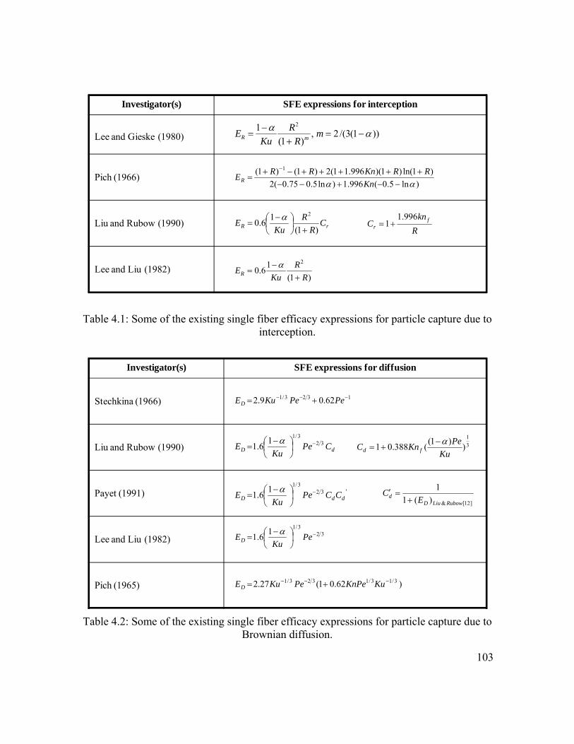
103

Investigator(s) SFE expressions for interception

Lee and Gieske (1980)

Pich (1966)


Lee and Liu (1982)

)ln5.0(996.1)ln5.075.0(2)1ln()1)(996.11(2)1()1( 1

αα −−+−−+++++−+

=−

KnRRKnRRER

rR CR

RKu

E)1(

16.02

+⎟⎠⎞

⎜⎝⎛ −

=α

)1(16.0

2

RR

KuER +

−=

α

Rkn

C fr

996.11+=

))1(3/(2,)1(

1 2

αα−=

+−

= mR

RKu

E mR

Table 4.1: Some of the existing single fiber efficacy expressions for particle capture due to interception.

Investigator(s) SFE expressions for diffusion

Stechkina (1966)


Payet (1991)

Lee and Liu (1982)

Pich (1965)

1323/1 62.09.2 −−− += PePeKuED

323/116.1 −⎟

⎠⎞

⎜⎝⎛ −

= PeKu

EDα

dD CPeKu

E 323/116.1 −⎟

⎠⎞

⎜⎝⎛ −

=α 3

1

))1((388.01Ku

PeKnC fdα−

+=

'323/116.1 ddD CCPe

KuE −⎟

⎠⎞

⎜⎝⎛ −

=α

]12[&)(11

RubowLiuDd E

C+

=′

)62.01(27.2 3/13/1323/1 −−− += KuKnPePeKuED


Brownian diffusion.

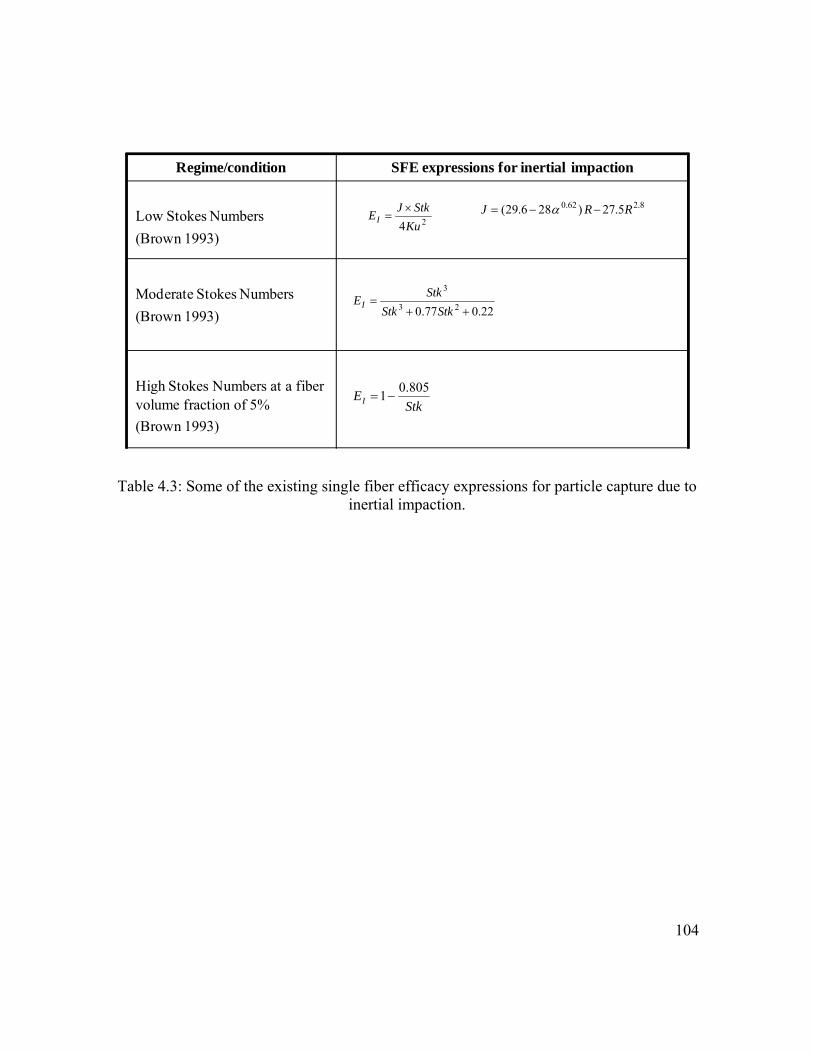
104

Regime/condition SFE expressions for inertial impaction

Low Stokes Numbers (Brown 1993)

Moderate Stokes Numbers(Brown 1993)

High Stokes Numbers at a fiber volume fraction of 5%(Brown 1993)

24KuStkJEI

×=

8.262.0 5.27)286.29( RRJ −−= α

StkEI

805.01−=

22.077.0 23

3

++=

StkStkStkEI

Table 4.3: Some of the existing single fiber efficacy expressions for particle capture due to inertial impaction.

105

CHAPTER 5. On the Importance of Fibers’ Cross-Sectional Shape for Air Filters Operating in the Slip Flow Regime♣

5.1. Introduction

With the recent advancements in electrospinning and melt-blowing processes, the

production of nanofibers is becoming increasingly viable (even though the term nanofiber

should in principle be used for fibers with a diameter smaller than 100 nanometers, it is a

common practice in the filtration community to use this term for fibers smaller than one

micrometer, and for the sake of convenience, we follow this convention here). Nanofibers

can significantly improve the performance of an ordinary air filter thanks to their minute

dimensions, which promote a phenomenon called aerodynamic slip. In a fibrous filter,

aerodynamic slip takes place when the fiber diameter is comparable to the mean free path

of the gas molecules (e.g., 65nm for air at normal temperatures and pressures). In such

conditions, collisions between the gas molecules and the fibers become so infrequent that

the gas can no longer be considered a continuum phase with respect to the fibers.

Aerodynamic slip results in a significant decrease in the drag force exerted on a fiber. This

leads to a lower pressure drop caused by a filter comprised of nanofibers when compared

to another filter with the same collection efficiency, but made up of microfibers.

• ♣Content of this chapter is published in an article entitled “On the Importance of Fibers’ Cross-

Sectional Shape for Air Filters Operating in the Slip Flow Regime” by Hosseini, S.A. and Tafreshi, H.V., Powder Technology 212 (3), 425-431 (2011).

106

The permeability and particle collection efficiency of nanofiber filter media have been

vastly studied in recent literature. Such studies include, but are not limited to, numerical

simulations of Maze et al. (2007), Hosseini and Tafreshi (2010,a,b,c), Wang and Pui

(2009), Wang et al. (2008), Zhao and Povitsky (2009); Przekop and Gradon (2008) as well

as the experimental work of Podgorski et al. (2006), Wang et al. (2008), and Shin and

Chase (2004). Since the infancy of filtration theory about fifty years ago, fibers have

always been assumed to be circular. There are many analytical, numerical, and empirical

correlations that have been developed for filters made up of circular fibers. There are also a

few studies dealing with non-circular microfibers (i.e., fibers with diameters greater than a

few micrometers), such as the work of Lamb and Costanze (1980), and Sanches et al.

(2007), Raynor (2008), Fotovati et al. (2011a), Cheung et al. (2005), Dhaniyala and Liu

(1999). However, despite the abundant number of studies dealing with microfibers, no

work has been dedicated to exploring the performance of media made of non-circular

nanofibers. Our hypothesis in this work is that a fiber’s cross-sectional geometry becomes

significantly more important when the air is in the slip flow regime, as the streamlines tend

to better conform to the actual shape of the fiber in the presence of aerodynamic slip. Our

objective in this work is to highlight the importance of a fiber’s cross-sectional shape in

calculating a filter’s pressure drop and collection efficiency in slip and no-slip flow

regimes. We examine our hypothesis using numerical simulations, and we validate our

simulation results with published studies in the literature, if available. In the next section,

we briefly describe our governing equations, boundary conditions, and numerical schemes

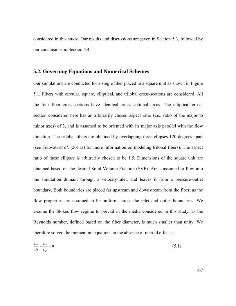
107

considered in this study. Our results and discussions are given in Section 5.3, followed by

our conclusions in Section 5.4.

5.2. Governing Equations and Numerical Schemes

Our simulations are conducted for a single fiber placed in a square unit as shown in Figure

5.1. Fibers with circular, square, elliptical, and trilobal cross-sections are considered. All

the four fiber cross-sections have identical cross-sectional areas. The elliptical cross-

section considered here has an arbitrarily chosen aspect ratio (i.e., ratio of the major to

minor axes) of 3, and is assumed to be oriented with its major axis parallel with the flow

direction. The trilobal fibers are obtained by overlapping three ellipses 120 degrees apart

(see Fotovati et al. (2011a) for more information on modeling trilobal fibers). The aspect

ratio of these ellipses is arbitrarily chosen to be 1.5. Dimensions of the square unit are

obtained based on the desired Solid Volume Fraction (SVF). Air is assumed to flow into

the simulation domain through a velocity-inlet, and leaves it from a pressure-outlet

boundary. Both boundaries are placed far upstream and downstream from the fiber, as the

flow properties are assumed to be uniform across the inlet and outlet boundaries. We

assume the Stokes flow regime to prevail in the media considered in this study, as the

Reynolds number, defined based on the fiber diameter, is much smaller than unity. We

therefore solved the momentum equations in the absence of inertial effects:

0=∂∂

+∂∂

yv

xu (5.1)

108

⎟⎟⎠

⎞⎜⎜⎝

⎛∂∂

+∂∂

=∂∂

2

2

2

2

yu

xu

xp µ (5.2)

⎟⎟⎠

⎞⎜⎜⎝

⎛∂∂

+∂∂

=∂∂

2

2

2

2

yv

xv

yp µ (5.3)

Our solution domains are meshed using uniformly distributed triangular elements. The

optimum mesh density, leading to mesh-independent simulation results (for both pressure

drop and collection efficiency results) for geometries such as those shown in Figure 5.1,

was obtained in our previous works (Hosseini and Tafreshi 2010c, Fotovati et al. 2011a).

A slip boundary condition has been considered in our calculations by enhancing the Fluent

CFD code with an additional C++ subroutine (User Defined Function, UDF). We used

Maxwell’s equation for the air velocity at the wall boundaries, as it relates the slip velocity

to the normal velocity gradient:

nuu

v

vw ∂

∂−= λ

σσ2 (5.4)

wherepdN

TR

ma22 π

λ = is the mean free path of gas molecules. In a previous publication, we

have demonstrated the accuracy of our implementation of the Maxell’s equation (see

Hosseini and Tafreshi 2010a).

We have used a Lagrangian particle tracking method in which the particle’s force balance

is integrated to obtain its position in time. The dominant forces acting on a particle are the

109

air drag force and the Brownian forces. For a particle Reynolds number smaller than unity,

we have (Li and Ahmadi 1992, Longest and Jinxiang 2007):

( ) )(182 tnuu

Cddtdu

ipcpp

p +−=ρµ (5.5)

( ) )(182 tnvv

Cddtdv

jpcpp

p +−=ρµ (5.6)

where the subscript p denotes properties associated with the particle. The first term on the

right hand side of this equation is the drag term, whereas the second term, )(tni , is the

Brownian force per unit mass defined as (Li and Ahmadi 1992, Longest and Jinxiang

2007):

tSGtn ii ∆

= 0)( π (5.7)

where 0S is the corresponding spectral intensity of the noise, given by (Li and Ahmadi

1992, Longest and Jinxiang 2007):

cpp CSdkTS 2520

216ρπ

ν= (5.8)

and iG is made by using the Muller-box method from two randomly chosen numbers

1U and 2U selected from a uniform distribution (Box and Muller 1958):

)2cos(ln2 21 UUGi π−= (5.9)

Fluent’s Discrete Phase Model (DPM) cannot correctly predict the particle trajectories

when the Brownian motion is included (Longest and Jinxiang 2007). We therefore

developed a UDF to redefine Equations (5.7) and (5.8) for the Fluent solver, and validated

110

our implementation in a previous work (Hosseini and Tafreshi 2010c). The Fluent’s DPM

also fails to recognize the actual size of a particle, and treats it as a point mass. We

therefore have also developed another UDF to include the actual dimensions of the

particles in detecting contacts between particles and wall boundaries (i.e., fibers), as they

are needed in the interception calculations (Hosseini and Tafreshi 2010 a,b).

Note that single fiber efficiency is the ratio of the number of particles captured by a fiber to

those injected from the projected area of the fiber at the inlet. In the absence of Brownian

forces (deterministic particle tracking), one can obtain the single fiber efficiency by

directly injecting particles from the above-mentioned projected area. With the Brownian

forces included, a different simulation strategy is needed. Particles that are captured by a

fiber due to Brownian diffusion are not necessarily those whose streamlines pass through

the projected area of the fiber at the inlet. In other words, particles from streamlines other

than those passing through the fiber’s projected area may diffuse into the volume that will

be swept by the fiber and get deposited. Similarly, particles originally passing through the

fiber’s projected area may change streamline, and penetrate through the filter. For this

reason, to calculate the fiber’s collection efficiency due to Brownian diffusion, we injected

particles from the entire inlet area, but counted only a fraction of the particles that were

injected from the inlet. This fraction is proportional to the ratio of the fiber’s projected area

to the total inlet area.

111

5.3. Results and Discussions

In this section, we present results of our fiber drag calculations conducted for square and

circular fibers with and without aerodynamic slip. We have also calculated the efficiency

of these fibers and compared them with one another, as will be seen later in this section.

5.3.1 Pressure Drop

Micro and nanofibers with different cross-sectional shapes but identical cross-sectional

areas are considered in this section. Figure 5.2 shows our fiber drag calculations for

nanofibers and microfibers (i.e., with and without the aerodynamic slip at the fiber surface,

respectively). The equation for fiber drag is given as:

2

( ) fdf p

Uhα

µ= ∆ (5.10)

The results shown in Figure 5.2a and 5.2b are obtained for circular fibers, and are also

compared with the predictions of an expression given by Brown (1993) for the drag force

on a fiber in a medium modeled with the 2-D cell model of Kuwabara (1959):

2

16 (1 1.996 )( , )

( 1.996 ( 0.5ln 0.25 0.25 ))f

ff

Knf Kn

Ku Knα

αα α

+=

+ − − + (5.11)

where 225.075.0ln5.0 ααα −+−−=Ku is the Kuwabara hydrodynamic factor, and

2 /f fKn dλ= is the fiber Knudson number. In Figure 5.2, delta and solid line (—), square

and dashed line (---), diamond and dash dotted line (-.-), left triangle and dotted line (…),

right triangle and long dashed line (– –), and gradient and dash dot-dotted line (-..)

represent solid volume fractions of 20%, 15%, 10%, 7.5%, 5%, and 2.5% , respectively.

112

Excellent agreement can be seen between our simulation results and Equation (5.11) with

and without slip effect. Note that significantly smaller fiber drag is obtained in presence of

aerodynamic slip.

Figure 5.2c and 5.2d, show the fiber drag exerted on square fibers. Note that, due to the

absence of any analytical or empirical correlations, these figures contain only the results of

our numerical simulations. It can again be seen that fiber drag is significantly reduced

when the slip effect takes place. It is interesting to note that fiber drag values increase with

increasing fiber diameter in the slip flow regime (Figure 5.2d). This is because Knudsen

number decreases with increasing fiber diameter, and the aerodynamic slip therefore

becomes increasingly less effective. Obviously, in the absence of the slip effect, fiber drag

is a constant value, only a function of SVF. Similar trends can be seen in Figures 5.2e

through 2h for fibers with trilobal and elliptical cross-sections.

The fiber drags in the slip flow regime (nanofibers) are normalized using their

corresponding fiber drag values obtained from microfiber simulations (no-slip flow

regime) /S NSf f for better comparison (see Figure 5.3). Note that NSf values are constant

for each fiber cross-sections. For the case of circular fibers, we have also added the

predictions of Equation (5.11) for validation purposes. Similar to Figure 5.2, delta and

solid line (—), square and dashed line (---), diamond and dash dotted line (-.-), left triangle

and dotted line (…), right triangle and long dashed line (– –), and gradient and dash dot-

dotted line (-..), represent solid volume fractions of 20%, 15%, 10%, 7.5%, 5%, and 2.5% ,

113

respectively. In Figure 5.3, note that the aerodynamic slip has a stronger influence on the

fiber drag at higher SVFs. This is due to the fact that, at higher SVFs, a greater portion of

the flow domain is influenced by the boundary layers formed around the fibers. Comparing

Figures 5.3a through 5.3d, it can be seen that aerodynamic slip more favorably influences

the pressure drop caused by the elliptical fibers. The cross-section least benefited by the

aerodynamic slip is the square geometry. This indicates that cross-sections which are more

streamlined with respect to the flow direction can better benefit from the favorable effects

of aerodynamic slip. In other words, in cross-sections where there is a large stagnation

region in front of the fiber (e.g., square or trilobal geometry), being in the slip flow regime

does not lead to significant drag reduction. To better demonstrate how streamlines come in

close vicinity of the fibers and conform to them in the slip flow regime, we have plotted

the streamlines around different nano- and microfibers in Figure 5.4. All nano- and

microfibers shown in this figure have an identical cross-sectional area, and are placed in a

cell with a SVF of 10.0%.

It is worth mentioning that we have also calculated /S NSf f in domains comprised of

more than 200 randomly distributed fibers similar to those reported by Hosseini and

Tafreshi (2010c) or Fotovati et al. (2011a) to ensure that the reported values are not valid

only for simulations conducted with one single fiber (results not shown). The /S NSf f

values obtained from multi-fiber simulations deviate less than 6% on average from those

114

reported in Figure 5.3, indicating that the simulations reported in this paper can correctly

represent the flow field in more realistic fibrous domains.

5.3.2 Collection Efficiency


filter medium. These are interception, inertial impaction, and Brownian diffusion. There

are different semi-empirical correlations that have been developed by different researchers

over the past fifty years to estimate the collection efficiency of fibrous filters with different

mean fiber diameters (Spurny 1998, Brown 1984). We have previously reported a

comprehensive comparison between predictions of these correlations along with those of

our 2-D and 3-D simulations (Hosseini and Tafreshi 2010c). Correlations of Liu and

Rubow (1990) are used in this study as they cover both slip and no-slip flow regimes and

are fairly accurate. Equations of Liu and Rubow (1990) for different capture mechanisms

are as follows:

rR CR

RKu

E)1(

16.02

+⎟⎠⎞

⎜⎝⎛ −

=α (5.12)

dD CPeKu

E 323/116.1 −⎟

⎠⎞

⎜⎝⎛ −

=α (5.13)

where fp ddR /= and Peclet number DVdPe f /= . The correction factors rC and dC are

defined as follows:

1.9961 f

r

KnC

R= + (5.14)

115

31

))1((388.01Ku

PeKnC fdα−

+= (5.15)

The total Single Fiber Efficiency is given as (Hinds 1999):

)1)(1(1 dR EEE −−−=∑ (5.16)

Our collection efficiency results are shown in Figure 5.5a through 5.5d for circular and

square fibers. The fibers in Figure 5.5a and 5.5b are nanofibers, whereas those in Figure

5.5c and 5.5d are microfibers. Predictions obtained from correlations of Liu and Rubow

(1990) are also added to these figures for comparison. It can be seen that our results are in

good agreement with the existing correlations developed for media made up of circular

fibers. More importantly, note that the difference between the collection efficiencies

obtained using square and circular nanofibers (see Figure 5.5a and 5.5b) are negligibly

small. This is because the fibers and the particles (25 to 500 nm) are close to each other in

size, and the minute differences between the streamline patterns around the circular and

square fibers cannot significantly influence the particle collection rate which is

predominantly due to interception. Our collection efficiency results for the case of

microfibers (Figure 5.5c and 5.5d) also indicate that the particle collection efficiency is

only weakly dependent on the fiber shape. The only noticeable difference between the

performances of these fibers is for the case of Brownian particles. This can be explained by

considering the fact that surface area (perimeter in 2-D) of the square fibers is about 12%

greater than those of the circular fibers, and therefore, the capture efficiency of square

fibers against Brownian particles should be slightly higher.

116

We did not try to simulate the collection efficeincy of microfibers with elliptical or trilobal

cross-section as such studies have been perfromed and reported in the litrature previoulsy

(Wang and Pui 2008, Raynor 2008, and Fotovati et al. 2011a). Obviously, collection

efficiency of a circular microfiber is quite different from that of an elliptical or trilobal

fiber with high aspect ratios, as they possess very different projected frontal areas.

However, as long as the projected frontal areas of the fibers are not severely different from

one anther, the collection efficiency values are in close proximity of one another (see

Fotovati et al. (2011a) for more discussions). For the case of nanofibers with elliptical or

trilobal cross-sections, as discussed earlier, since the nanofibers are close in diameter to

aerosol particles of concern (25 to 500 nm), and the minute differences between the

streamline patterns around these fibers cannot significantly influence the particle collection

rate, which is chiefly due to interception.

5.4. Conclusions

Numerical simulation has been used in this study to compare the importance of fibers’

cross-sectional shapes on the performance of a fibrous filter in the slip and no-slip flow

regimes. The slip and no-slip flow regimes are those expected to prevail in fibrous media

made up of nanofibers (fibers with submicron diameters) and microfibers (fibers having a

diameter greater than few micrometers), respectively. In particular, we compared fibers

with square, circular, trilobal, and elliptical cross-sections at micro- and nanoscales to

conclude that the cross-sectional shape of the fibers has a more pronounced effect on a

117

filter operates in the slip flow regime (made up of nanofibers) and the fibers have more a

streamlined shape. The fiber geometry was found to be more important in pressure drop

prediction rather than capture efficiency estimation.

118

inle

tin

let

inle

tin

let

outle

tou

tlet

outle

tou

tlet

symmetry

symmetry

Figure 5.1: Computational domain considered for modeling flow around square and circular fibers.

119

df (µm)

f cirN

S

2 3 4 5 6 7 8

0

5

10

15

df (µm)

f sqNS

2 3 4 5 6 7 8

0

5

10

15

df (nm)

f ellS

200 300 400 500 600 700 800

0

2

4

6

8

df (nm)

f triS

200 400 600 8000

5

10

15

20

df (nm)

f cirS

200 300 400 500 600 700 800

0

5

10

15

df (nm)

f sqS

200 400 600 800

0

5

10

15

df (µm)

f triNS

2 3 4 5 6 7 80

5

10

15

20

a) b)

c) d)

df (µm)

f ellN

S

2 3 4 5 6 7 8

0

2

4

6

8

e) f)

g) h)

Figure 5.2: Fiber drag in the no-slip and slip flow regimes are calculated for circular (a and b), square (c and d), trilobal (e and f), and elliptical (g and h) fibers. For the case of circular fibers, simulation results (symbols) are compared with the predictions of Equation (5.11) (lines). Delta

and solid line (—), square and dashed line (---), diamond and dash dotted line (-.-), left triangle and dotted line (…), right triangle and long dashed line (– –), and gradient and dash dot-dotted line (-..),

represent solid volume fractions of 20%, 15%, 10%, 7.5%, 5%, and 2.5% , respectively.

120

df (nm)

f ellS /f el

lNS

200 400 600 8000.5

0.6

0.7

0.8

0.9

1df (nm)

f sqS /f sqNS

200 400 600 8000.5

0.6

0.7

0.8

0.9

1a) b)

c) d)

df (nm)

f cirS /f ci

rNS

200 400 600 8000.5

0.6

0.7

0.8

0.9

1

df (nm)

f triS /f triNS

200 400 600 8000.5

0.6

0.7

0.8

0.9

1

Figure 5.3: Slip-to-no-slip fiber drag ratios are calculated for circular (a), square (b), trilobal (c), and elliptical (d) fibers. For the case of circular fibers, simulation results

(symbols) are compared with the predictions of Equation (5.11) (lines). Delta and solid line (—), square and dashed line (---), diamond and dash dotted line (-.-), left triangle and

dotted line (…), right triangle and long dashed line (– –), and gradient and dash dot-dotted line (-..), represent solid volume fractions of 20%, 15%, 10%, 7.5%, 5%, and 2.5% ,

respectively.

121

10 µm 100 nm

b)a)

d)c)

f)e)

h)g)

Figure 5.4: Streamlines around circular (a and b), square (c and d), elliptical (e and f), and trilobal (g and h) fibers in no-slip and slip flow regimes (i.e., microfiber and nanofibers,

respectively). Note how streamlines conform to the fiber’s perimeter in the slip flow regime.

122

dp (nm)

Sing

leFi

berE

ffic

ienc

y

100 300 500 7000

0.05

0.1

0.15

0.2

0.25Circular fiber (no-slip flow)Square fiber (no-slip flow)Liu & Rubow (1990)

df = 6 micron

SVF=10%

dp (nm)

Sing

leFi

berE

ffic

ienc

y

100 300 500 7000

0.05

0.1

0.15

0.2

0.25Circular fiber (no-slip flow)Square fiber (no-slip flow)Liu & Rubow (1990)

df = 8 micron

SVF=10%

dp (nm)

Sing

leFi

berE

ffic

ienc

y

100 300 500 700

0.5

1

1.5

2

2.5Square fiber (slip flow)Circular fiber (slip flow)Liu & Rubow (1990)

df = 200 nm

SVF=10%

dp (nm)

Sing

leFi

berE

ffic

ienc

y

100 300 500 700

0.5

1

1.5

2

2.5Square fiber (slip flow)Circular fiber (slip flow)Liu & Rubow (1990)

df = 400 nm

SVF=10%

a)

c)

b)

d)

Figure 5.5: Single fiber collection efficiency calculated for fibers with a diameter of 200 nm (a), 400 nm (b), 6 µm (c), and 8 µm (d), at a solid volume fraction of 10%. A

comparison is made between the efficiency of fibers with circular and square cross-sections.

123

CHAPTER 6. Modeling Particle-Loaded Single Fiber Efficiency

and Fiber Drag using Fluent CFD Code♣

6.1- Introduction Classical theories of particle filtration via fibrous filters have been developed for clean

media. These theories have been based on an exact or numerical solution of the flow field

around a perfectly clean fiber placed normal to the flow direction in a two-dimensional

configurations (Brown 1993, Spurny 1998). Classical filtration theories have resulted in a

variety of easy-to-use semi-empirical expressions for predicting the performance (i.e.,

collection efficiency and pressure drop) of filter media (see Brown 1993, Spurny 1998 for

comprehensive reviews). However, filters do not remain clean during the course of their

operation. Particles deposit on the fibers and form complicated dendrite structures. The

deposited particles affect the flow field around a fiber as the air streamlines change in

response to the changes in the filter’s morphology, and render the aforementioned

expressions inaccurate. Therefore, existing pressure drop and collection efficiency

expressions are only valid for the early stages of a filter’s lifecycle.


provide accurate predictions for the performance of particle-loaded filter media. The most

♣Content of this chapter is submitted for publication by Hosseini, S.A. and Tafreshi, H.V. in an article entitled “Modeling Particle-Loaded Single Fiber Efficiency and Fiber Drag using Fluent CFD Code”.

124

computationally-affordable approach to account for the changes in a filter’s internal

structure is to assume that the deposited particles form a 2-D homogenous porous coating

with a given porosity and particle size around the fibers, and to allow this coating to grow

according to some simple mathematical rules. However, such an approach comes at the

expense of neglecting the microstructure of particle deposits, which can lead to

considerable errors in predicting the flow streamlines, and therefore collection efficiency

and pressure drop, especially for the particles captured via interception or inertial

impaction mechanisms (e.g., Giuliani and Vafai 1999, Steffens and Coury 2007, Dunnett

and Clement 2009). As will be discussed later in this paper, a more realistic model of a

particle loading process is one that captures the dendrite shape of the deposits and updates

the flow field based on such morphological changes.

The shape of a loaded fiber changes depending on the particle deposition regime. If the

deposition mechanism is mainly interception, the deposit pattern will be on the fibers’

lateral sides. By increasing the Stokes number ( fcpp dVCdStk ηρ 18/2= ), the mode of

particle deposition changes to inertial impaction. In this case, the particle does not follow

the streamlines perfectly, and instead travels on a straight path, depositing on the fiber’s

front side. Note that particles which are deposited on the lateral sides of a fiber cause a

much higher pressure drop than those deposited on the fiber’s front side. Particle

deposition due to Brownian diffusion is believed to form uniform deposits all around the

fiber, as the inertial effects are negligible.

125

Most filtration theories are developed using a so-called Single Fiber Efficiency (SFE)

which describes the efficiency of a single fiber in collecting particles from a particle-

loaded stream. SFE can be calculated by placing a fiber perpendicular to the flow inside a

cell that resembles the influence the neighboring fibers. The size of the cell with respect to

the fiber can resemble Solid Volume Fraction (SVF) of the filter. Although, it is a very

simplified version of filter flow; This suggested method by Kuwabara (1959) gives us an

acceptable prediction. Some of its limitations are: All fibers in the filter have the same flow

field and they are perpendicular to main flow direction. By using this geometry Kuwabara

solved two dimensional viscous flow equations and obtained the velocity profile around

fiber. In Kuwabara cell model, the stream function ψ can be obtained by solving the

biharmonic equation in cylindrical polar coordinate.

With the SFE information and cell dimensions, one can estimate the collection efficiency

of a filter medium using the expression given in the literature (see Brown 1993, Spurny

1998). Similarly, the pressure drop caused by a filter medium can be obtained if the drag

force exerted by the flow on a single fiber, i.e., fiber drag, is known. In a pioneering work,

Payatakes and Tien (1976) simulated chain-like dendrite growth on fibers orderly placed

within a Kuwabara cell. For simplicity, they considered interception to be the only particle

collection mechanism. They also chose the size of their computational grids to be equal to

the diameter of the particles, which could have affected the accuracy of their results, as

will be discussed later in this paper. Later on, Payatakes and Gradon (1980) modified this

126

model to also include particle capture via diffusion and inertial impaction mechanisms.

Utilizing the Monte Carlo technique in a Kuwabara cell, Kanaoka et al. (1980) calculated

the SFE for particles in the inertial and interception regimes. They simulated the growth of

particle dendrites on a fiber to propose new formulas for predicting the loaded-to-clean

SFE using a linear relationship:

0

1E ME

γ− = (6.1)

Kanaoka et al. (2001) and Cheung et al. (2005) reported on case studies in which particle

deposition on electret fibers placed in constant flow fields were numerically simulated.

Nevertheless, in neither of the above studies (i.e., Payatakes and Tien 1976, Payatakes and

Gradon 1980, Kanaoka et al. 2001, and Cheung et al. 2005) was the air flow field

recalculated during the particle deposition process, leading to an overestimation of the

fiber’s collection efficiency, as demonstrated by Filippova and Hanel (1997), who

developed a Lattice-Boltzmann model of flow around two (and three) crossing fibers. As

will be discussed later in this paper, the air flow field should be updated during the deposit

formation as frequently as possible to correctly simulate the instantaneous flow field and

consequently the growth of the dendrite structures. Przekop et al. (2003) also used the

Lattice-Boltzmann method to simulate particle deposition on a fiber. These authors

recalculated the flow field around the fiber after particle deposition. However, their

simulations were conducted in 2-D domains which significantly affected accuracy of their

pressure drop and collection efficiency calculations. The work of Filippova and Hanel

(1997) was later extended to simulate deposition of nanoparticles under an electrostatic

127

field by Lantermann and Hanel (2007). Unlike the work of Kanaoka et al. (1980,2001),

flow field recalculation was considered in the work of Filippova and Hanel (1997) and

Lantermann and Hanel (2007) for improving accuracy. Filippova and Hanel (1997) and

Lantermann and Hanel (2007), however, did not propose any correlations like that given in

Equation 6.1.

Among different numerical techniques, the Discrete Element Method (DEM) has also been

used for modeling particle deposition on a fiber’s surface. In a recent study, Li and

Marshall (2007) modeled particle loading in 3-D domains using DEM in a constant flow

field to demonstrate their model’s capabilities. These authors, however, neither reported

any pressure drop data nor discussed the morphology of their simulated particle dendrites.

With the recent progress made in the field of Computational Fluid Dynamics (CFD) and

the availability of fast and reliable general-purpose commercial CFD packages, it is now

more plausible to take advantage of the current state of the art in CFD modeling rather than

developing an in-house code for each and every fluid flow problem. Such commercial

packages, however, may need additional subroutines to enhance their capabilities and

customize their features for a given specific modeling task. The goal of the current paper is

to present a methodology for predicting the fiber drag and SFE during the particle loading

process using the Fluent CFD code (as mentioned, earlier a filter’s pressure drop and

collection efficiency can be obtained from fiber drag and SFE). We describe and

demonstrate our in-house subroutines that allow one to track particles of different sizes,

128

and simulate formation of 3-D dendrite particle deposits on the surface of a fiber(s). Our

simulation techniques and in-house subroutines are discussed in the next section. A series

of simulations demonstrating the growth of particle dendrites and their influence on fiber

drag and SFE is given in Section 6.3, followed by our conclusions in Section 6.4.

6.2. Modeling Particle-Loaded Filter Media In this section, we first discuss how the air flow field around a fiber is modeled in our

simulations. We then discuss our techniques for simulating particle flow though the

domain, and eventually present our algorithm for simulating particle deposition and

dendrite formation.

6.2.1. Flow Field Calculations

In this study, a single fiber is placed on the center of a square cell with the boundary

conditions shown in Figure 6.1. The size of the cell is chosen according to the targeted

SVF. An inlet region with a length of 20 fd is considered upstream of the fiber to ensure

that the assumption of uniform flow field at the inlet is accurate. The air flow throughout

the domain is assumed to be laminar as the Reynolds number, defined based on the fiber

diameter, is smaller than unity. The finite volume method implemented in the Fluent code

is used to solve the continuity and momentum equations in the absence of inertial effects:

0u v wx y z∂ ∂ ∂

+ + =∂ ∂ ∂

(6.2)

129

2 2 2

2 2 2p u u ux x y z

µ⎛ ⎞∂ ∂ ∂ ∂

= + +⎜ ⎟∂ ∂ ∂ ∂⎝ ⎠

(6.3)

2 2 2

2 2 2p v v vy x y z

µ⎛ ⎞∂ ∂ ∂ ∂

= + +⎜ ⎟∂ ∂ ∂ ∂⎝ ⎠

(6.4)

2 2 2

2 2 2p w w wz x y z

µ⎛ ⎞∂ ∂ ∂ ∂

= + +⎜ ⎟∂ ∂ ∂ ∂⎝ ⎠

(6.5)

Air enters the domain with a constant velocity and leaves it with constant pressure. The

symmetry boundary condition is assumed for the sides of the domain. The slip boundary

condition is considered on the fiber's surface. Aerodynamic slip is known to take place

when the fiber diameter is comparable in size to the mean free path of the molecules in the

surrounding gas. Slip flow is often characterized by calculating the Knudsen

number, 2 /f fKn dλ= , where 2/ ( 2 )a mRT N d pλ π= is the mean free path of gas molecules.

A continuum flow regime is assumed to prevail in a fibrous medium when 310fKn −< .

When 310fKn −> , the no-slip boundary condition no longer applies to the fiber’s surface.

For the most practical range of fiber diameters at the normal atmospheric conditions,

Knudsen number falls in range of ( 3 110 2.5 10fKn− −< < × ), which corresponds to the so-

called slip-flow regime (Brown 1993, Spurny 1998).

Using the Maxwell’s first order model, we have developed a C++ User-Defined Function

(UDF) that runs in the Fluent environment and modifies the wall shear stress for

130

simulations conducted under a slip-flow regime (McNenly et al. 2005, Duggirala et al.

2008)

2 vw

v w

uun

σλ

σ− ∂

=∂

(6.6)

By using equation 6.6 and the definition of wall shear stress; the slip velocity has been

defined as:

2 vw w

vu σλτ

µ σ−

= (6.7)

Gambit, a preprocessor for the Fluent code, is utilized to mesh the flow domain using

tetrahedral elements, refined close to the fiber surfaces. The mesh size has been chosen in a

way that volume of each particle is covered by some 8-12 cells in the domain. For

example, for a particle diameter of 8µm, a mesh size of about 3µm or smaller has been

used for accuracy. Obviously, accuracy of the simulations can be further improved by

using smaller mesh sizes. However, since the focus of the current paper is mostly on the

methodology rather than absolute numerical values of fiber drag or SFE, we did not

attempt to assess the influence of mesh density on the results presented here. Nevertheless,

we believe that the mesh sizes used in this study are good enough to produce reliable

quantitative conclusions such as those presented in Sections 6.3.1 and 6.3.2. In a previous

study we showed that 25 grid points around the circular perimeter of a fiber can be

sufficient for simulating pressure drop and collection efficiency of a clean filter with

reasonable accuracy (Hosseini and Tafreshi 2010b). Therefore, attention has been paid to

131

ensure that the choice of mesh size results in more 25 grid points on the fiber circular

perimeter in the simulations reported here (see also Hosseini and Tafreshi 2010c, Fotovati

et al. 2010, Hosseini and Tafreshi 2010a, Tahir and Tafreshi 2009 for more information).

6.2.2. Modeling Particle Capture and Deposition on Fibers

Particle trajectory calculations have been conducted via the Lagrangian method. The SFE

is defined as the ratio of the number of particles captured by a fiber to that injected from

the projected area of the fiber at the inlet. In our simulations, groups of particles have been

injected from random points within the projected image of the fiber on the inlet boundary.

Random particle injection is important in generating realistic dendrite shapes because

injecting particles from the same injection sites results in formation of unrealistic chain-

like particle dendrites (similar to those of Payatakes and Tien 1976).

It is important to note that in the case of Brownian particles (particles smaller than 500nm)

a different simulation strategy is needed. Particles that are captured by a fiber due to

Brownian diffusion are not necessarily those whose streamlines pass through the projected

area of the fiber at the inlet. In other words, particles from streamlines other than those

passing through the fiber’s projected area may diffuse into the volume that will be swept

by the fiber, and get deposited. Similarly, particles originally passing through the fiber’s

projected area may change streamline, and penetrate through the filter. For this reason, to

calculate the SFE due to Brownian diffusion, we injected particles from the entire inlet

132

area, but counted only a fraction these particles, with the fraction being the ratio of the

fiber’s projected area to the total inlet area.

The particle trajectories have been calculated by integrating the force balance on the

particle. There are two types of forces applied to the particle, drag force and Brownian

force, together represented by:

( )218 ( )p

p ip p c

duu u n t

dt d Cµ

ρ= − + (6.8)

( )218 ( )p

p jp p c

dvv v n t

dt d Cµ

ρ= − + (6.9)

( )218 ( )p

p kp p c

dww w n t

dt d Cµ

ρ= − + (6.10)

Brownian force per mass is defined by ( )in t in equation (6.8-6.10). It is a function of time

step, temperature, particle diameter and material and fluid viscosity which is (Longest and

Xi 2007, Li and Ahmadi 1992):

0( )i iSn t Gt

π=

∆ (6.11)

where iG has a zero mean and a unit variance chosen from a normal distribution, and 0S is

the corresponding spectral intensity of the noise given by (Longest and Xi 2007, Li and

Ahmadi 1992):

0 2 5 2216

p p c

TSd S Cνσ

π ρ= (6.12)

133

The above equations are programmed in the form of a UDF to introduce a correct

Brownian diffusion to Fluent’s discrete phase module. The validation of this work is

presented in our previous publications (Hosseini and Tafreshi 2010c).

The Fluent code models a particle as a point mass, and is unable to detect a collision

between a fiber and a particle unless the particle’s center of mass touches the fiber. While

this approximation may be accurate for defining a contact between a particle and a

macroscopically large object, it is not appropriate for calculating particle capture via

interception with a fiber. Similarly, Fluent’s discrete phase module cannot detect a

collision between a particle and previously deposited particles. To do this, one needs to

record the coordinates of the particles that have already been deposited. When the distance

between a particle and the fiber or the surface of another already deposited particle is

smaller than particle radius, particle velocity should be set equal to zero, i.e., particle

position should be fixed. For modeling a deposited particle, it should be saved as part of

the solid structure to so that it can be reused for flow field recalculation and forming

particle dendrite.

In our study, two User Defined Memories (UDMs), hereon called UDM0 and UDM1, have

been defined for the Fluent code to be used in simulating the dendrite stricture created by

particle deposition. We start by assigning a zero to the UDM0 value of any computational

cell that does not contain any particle. If the cell becomes filled with a deposited particle,

we then change its UDM0 value to unity. We call this procedure “cell marking”. Cell

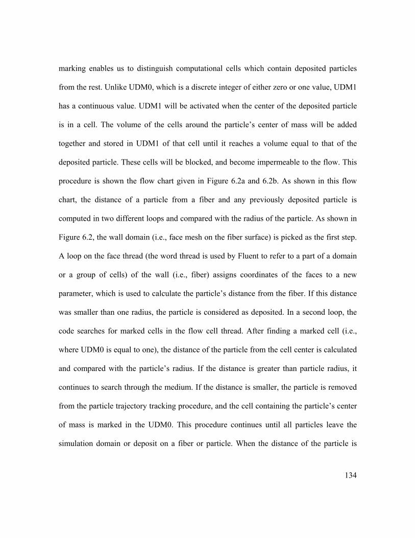
134

marking enables us to distinguish computational cells which contain deposited particles

from the rest. Unlike UDM0, which is a discrete integer of either zero or one value, UDM1

has a continuous value. UDM1 will be activated when the center of the deposited particle

is in a cell. The volume of the cells around the particle’s center of mass will be added

together and stored in UDM1 of that cell until it reaches a volume equal to that of the

deposited particle. These cells will be blocked, and become impermeable to the flow. This

procedure is shown the flow chart given in Figure 6.2a and 6.2b. As shown in this flow

chart, the distance of a particle from a fiber and any previously deposited particle is

computed in two different loops and compared with the radius of the particle. As shown in

Figure 6.2, the wall domain (i.e., face mesh on the fiber surface) is picked as the first step.

A loop on the face thread (the word thread is used by Fluent to refer to a part of a domain

or a group of cells) of the wall (i.e., fiber) assigns coordinates of the faces to a new

parameter, which is used to calculate the particle’s distance from the fiber. If this distance

was smaller than one radius, the particle is considered as deposited. In a second loop, the

code searches for marked cells in the flow cell thread. After finding a marked cell (i.e.,

where UDM0 is equal to one), the distance of the particle from the cell center is calculated

and compared with the particle’s radius. If the distance is greater than particle radius, it

continues to search through the medium. If the distance is smaller, the particle is removed

from the particle trajectory tracking procedure, and the cell containing the particle’s center

of mass is marked in the UDM0. This procedure continues until all particles leave the

simulation domain or deposit on a fiber or particle. When the distance of the particle is

135

smaller than the radius, the particle’s center of mass is exported to a file for further

analysis.

A method is developed to capture the spherical shape of the particle. This technique is used

as a subroutine block in Figure 6.2a and the detailed explanation is given in Figure 6.2b.

Centered on the cell containing the particle’s center of mass, we consider a sphere with a

diameter of 0.3 pd , and grow it to cover as many neighboring cells as needed to make up a

volume equal to that of the deposited particle. In this process, we allow the sphere to grow

with an increment of 0.05 pd in radius (see Figure 6.3). Note that this is made possible by

considering cells smaller than the particles. In order to resolve the spherical shape of a

particle, we first change the UDM1 value of the cell that contains the particle’s center of

mass to the cell’s volume. We then add the volumes of the neighboring cells to the volume

of the specified cell (i.e., its UDM1) which contained the particle’s center. In this

procedure, our UDF searches for unused cells having a UDM0 value of zero. Thus, we

increase the UDM1 value of that cell by adding the volume of the unmarked surrounding

cells until it reaches the same volume as the particle. After this procedure is completed, the

UDM0 value of the cells associated with the particle should be changed to one to specify

them as “filled”. This process is required due to the non-uniform mesh size across the

medium. Note that this algorithm enables us to have different particle sizes without

needing to re-mesh the geometry, unlike in the work of Kanaoka et al. (1980). With this

136

procedure, one can use a very fine mesh size to perfectly capture the spherical shape of the

deposited particles.

After marking the cells occupied by the deposited particles in the flow domain, we increase

the cells’ viscosity by two orders of magnitudes and set their flow velocity equal to zero.

Note that a sudden increase in the viscosity of neighboring cells can cause numerical

instability or divergence. To help with stabilizing the simulations, we enforced a maximum

allowable fluid velocity equal to 20 times the velocity at the inlet. The cell blocking

procedure was executed after deposition of each batch of particles. A C++ subroutine was

written to change the viscosity and limit the maximum velocity in these cells.

In our simulations, the flow field has been recalculated before the total volume of

deposited particles reaches 5% of the volume of the fiber. As we cannot control the number

of loaded particles due to both the random motion and random injection of the particles,

this was controlled instead by limiting the number of particles at injection by trial and

error.


6.3.1. Particle Dendrite Formation

The shape of particle dendrites changes depending upon the flow and particle regimes.

There are three major mechanisms for particle capture: Brownian diffusion, inertial

impaction, and interception. When the dominant capture mechanism is interception,

137

particles tend to deposit on the sides of the fiber with respect to the stagnation point. In the

interception-dominant regime, deposition of each single particle can affect the filter’s

pressure drop as the growth of dendrites tend to rapidly increase the fiber’s cross-sectional

area normal to the flow direction. This is somewhat in contrast to the way particle

dendrites grow when inertial impaction is the dominant capture mechanism. In that case,

particles tend to deposit around the stagnation point. This is because inertial particles do

not follow their streamlines perfectly at the turns and instead tend to travel on a straight

path to deposit on the fiber’s front side. In the inertial impaction regime, growth of particle

dendrites does not significantly influence the fiber’s cross-sectional area normal to the flow

direction, and consequently, the rate of increase of pressure drop in this regime is expected

to be minimal. Note that the rate of increase in collection efficiency is also minimal in this

regime for the same reason.

Figure 6.4a shows an example of when the dominant capture mechanism is interception.

The fiber shown in this figure has a diameter of 4fd mµ= and is loaded with particles

having a diameter of 250pd nm= . The fiber is placed in a cell with a solidity of 5%.

Similarly, Figure 6.4b shows an example of when the dominant capture mechanism is

inertial impaction with a fiber having a diameter of 20fd mµ= loaded with particles with a

diameter of 2000pd nm= and placed in a cell with a solidity of 3%. Our results, shown in

Figure 6.4a and 6.4b, are in good qualitative agreement with the observations of Kasper et

al. (2009,2010) who conducted a series of experiments to study the structure of particle

138

dendrites made up of particles with diameters in the range of 1.3-5.2 µm (i.e., relatively

large particles).

Particle deposition due purely to Brownian diffusion is believed to form uniform deposits

all around the fiber, as the inertial, geometrical, and hydrodynamic effects are negligible

when particles are extremely small (a few nanometers in diameter). Particle dendrites

formed because of Brownian diffusion often have many branches distributed in the radial

direction. If the particles are small enough to exhibit Brownian diffusion, but at the same

time sufficiently large to be affected by the flow field (e.g., 50 nm), then the shape of the

particle deposit will look like a combination of the dendrites expected from purely

Brownian particles and those caused by pure interception. An example of a situation like

this is shown in Figure 6.4c, where particles with a diameter of 75pd nm= are deposited on

a fiber having a diameter of 1fd mµ= in a cell with a solidity of 5%.

6.3.2. Fiber Drag and Collection Efficiency of Particle-Loaded Fibers

In this section, we discuss the rate of change of pressure drop and collection efficiency of a

single fiber during loading. Figure 6.5 shows the average single fiber efficiency E

normalized by the efficiency of the clean fiber. The average efficiency was calculated by

dividing the number of loaded particles by the total number of particles injected into the

domain. The x-axis in the plots shown in Figure 6.5 is the mass of loaded particles in

kilograms divided by the volume of the cell (see equation 6.1):

139

3 3

2 2

2 23 3

p p pp

f f

N d NdM

d l d lαρ π

αρπ

= = (6.13)

Our results indicate that the normalized efficiency increases with increasing mass of the

loaded particles M. However, the rate of increase of efficiency is not always constant, as

expected from the expression proposed by Kanaoka et al. (1980), i.e., Equation 6.1. Our

results indicate that the rate of increase of normalized efficiency decreases with increasing

M until it becomes constant, resulting in a linear relationship, as expected from Equation

6.1. The reason for this seems to be the fact that the growth of a fiber’s normal cross-

section (normal to the flow direction) relative to its original value is faster at the initial

stages of the particle loading process. Of course, the onset of the linear region depends on

the flow, fiber, and particle properties. A similar effect has also been observed in the

experiments of Kasper et al. (2009, 2010) with larger particles. In our analysis, we only

used the linear portion of the plots shown in Figure 6.5 for curve fitting. The line equation

is presented as:

01E a bM

E− = + (6.14)

where the a and b (in m3/kg) values are shown in Figure 6.5 for each case.

In Figure 6.6, normalized fiber drag is plotted versus mass of the loaded particles for the

same fibers and particles discussed in Figure 6.5. It can be seen that fiber drag increases

exponentially with increasing deposited mass. The increase in the fiber drag is because of

the increase in the size and change in shape of the fibers with respect to their neighboring

fibers (i.e., the unit cell). Note that when plotted against the mass of deposited particles,

140

the rate of increase in fiber drag is higher for smaller particles. This is simply because

more particles are needed to form a dendrite with a given mass when the particle diameter

is smaller. Therefore, a dendrite made up of small particles is much larger than one with

the same mass, composed of larger particles. Note also that a dendrite produced in the

interception regime can cause a greater pressure drop than a dendrite made due to inertial

impaction, as the latter is better streamlined. The general exponential format is considered

for normalized fiber drag as:

0 ehMd

d

f qf

= (6.15)

Values of q and h are obtained via curve fitting and are shown in Figure 6.6. To better

simulate the loading of particles on a fiber under inertial impaction, we considered a fiber

with a diameter of 20µm in a cell with a solidity of 5% challenged with particles having a

diameter of 2µm (see Figure 6.7). As can be seen in Figure 6.7a, normalized fiber drag

increases almost linearly with increasing mass of loaded particles. This effect can be due to

the fact that the loaded particles are mostly deposited on the front side of the fiber, and so

they do not significantly increase the fiber’s cross-section normal to the flow direction.

Figure 6.7b shows that in this case, the fiber’s collection efficiency remains almost

invariant with time (mass of the deposit). This is again due to the fact that the particle

dendrites in the inertial regime tend to remain within the projected frontal area of the fiber.

Figure 6.8 presents the slope of the linear portion of the normalized single fiber efficiency

plots shown in Figure 6.5. It can be seen that the slope decreases with increasing particle

141

diameter. As mentioned earlier, for a given mass of deposited particles, dendrites made up

of small particles are larger and cause more resistance to air flow. In Figure 6.8, it can also

be noted that the rate of single fiber efficiency increase in the case of particles having a

diameter of 50 nm is less than that of particles with a diameter of 75 nm. This effect is

believed to be attributed to the fact that the clean fiber efficiency 0E (see Figure 6.8b) is

smaller for particles with a diameter of 75nm, leading to higher normalized single fiber

efficiency 0/E E . Similar trends have also been reported by Myojo et al. (1984) and Kasper

et al. (2009,2010).

In Figure 6.9, we present the coefficient b of the exponential functions used for curve

fitting into the fiber drag plots shown in Figure 6.6. It can be seen that this coefficient

decreases with increasing particle diameter when the mass of the particle deposit is kept

constant, as discussed earlier.

6.4. Conclusions

This study was devised to demonstrate how one can enhance the capabilities of a

commercially available CFD code to simulate the challenging problem of unsteady-state

filter loading (aging), and predict the rate of change of pressure drop and collection

efficiency of the filter in the presence of aerodynamic slip. To accomplish this, a series of

in-house subroutines (UDFs) were developed in C++ and coupled with Fluent’s core

solver. In particular, simulation of particle collection due to interception and Brownian

142

diffusion, as well as dendrite formation on a fiber or any previously deposited particle, is

made possible by enhancing the capabilities of the Fluent code. Aerodynamic slip on the

fiber surface is also introduced to the simulations using another in-house subroutine for the

case of small fibers.

Considering a fiber with a diameter of 1µm exposed to flowing aerosol particles with

diameters ranging from 50 to 500 nm, we predicted series of correlations for the rate of

change of fiber collection efficiency and fiber drag as function of mass of loaded particles.

This study clearly shows that the rate of increase of collection efficiency and pressure drop

is higher for filters loaded with smaller particles, if the mass of the loaded particles is kept

constant. On the contrary, simulating a fiber having a diameter of 20µm loaded with

particles with a diameter of 2µm (where the capture mechanism is inertial impaction), we

observed almost no increase in the rate of particle collection efficiency, and a less

pronounced rate of pressure drop increase.

143

Inlet Symmetry Outlet

Cell

Figure 6.1: Simulation domain and the boundary conditions.

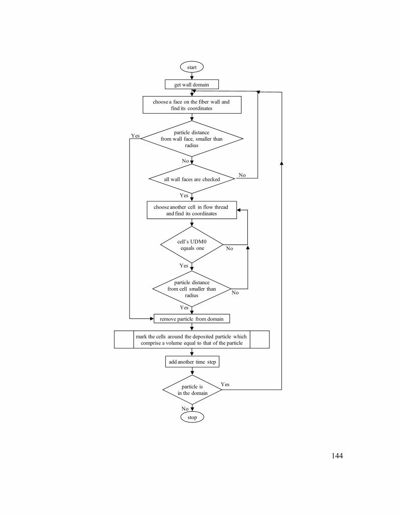
144

get wall domain

choose a face on the fiber wall and find its coordinates

particle distancefrom wall face, smaller than

radius

choose another cell in flow thread and find its coordinates

remove particle from domain

all wall faces are checked

start

add another time step

particle isin the domain

stop

No

Yes

Yes

Nocell’s UDM0

equals one

No

particle distancefrom cell smaller than

radius

Yes

No

mark the cells around the deposited particle which comprise a volume equal to that of the particle

Yes

No

Yes

145

replace the value of UDM1 with the volumeof the cell containing particle’s center

add volume of the cell to UDM1

UDM1 value is biggerthan particle volume

block the related cell which particle is in it by changing the value of UDM0 to 1

start

save the coordinates of deposited particle

search for another cell in criterion sphere

UDM0 value is zero

change the value of UDM0 to 1

stop

Yes

Yes

No

No

hasall cells in

criterion sphere counted?

increase the criteria sphere size

by 0.05dp

Yes

No

enter criterion sphere size (default is 0.3dp)

Figure 6.2: Flowchart of the particle loading subroutine (a) and the subroutine used for resolving the spherical shape of the deposited particles (b).

146

Figure 6.3: Two particles with a diameter of 200 nm loaded on a fiber with a diameter of 1µm. The particles are made up of a group of cells marked using the procedure described in Figure 6.2. Note that in generating this figure we have used a relatively fine mesh, for

better illustration.

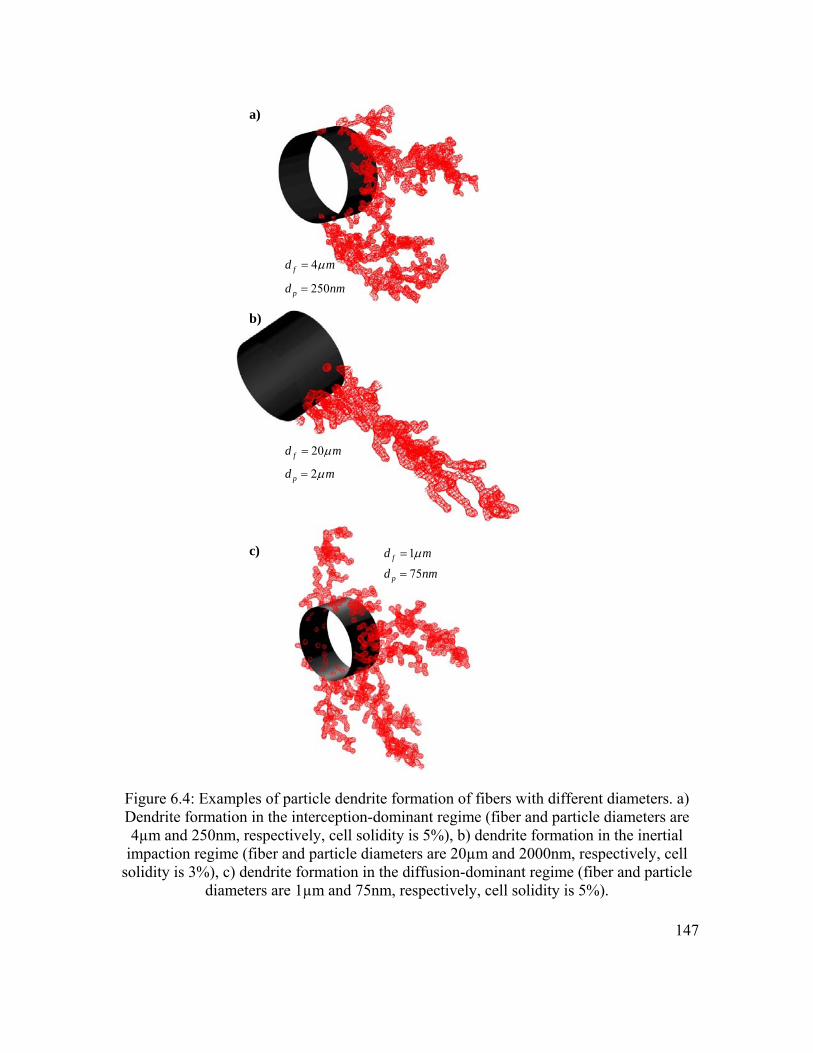
147

Figure 6.4: Examples of particle dendrite formation of fibers with different diameters. a) Dendrite formation in the interception-dominant regime (fiber and particle diameters are 4µm and 250nm, respectively, cell solidity is 5%), b) dendrite formation in the inertial

impaction regime (fiber and particle diameters are 20µm and 2000nm, respectively, cell solidity is 3%), c) dendrite formation in the diffusion-dominant regime (fiber and particle

diameters are 1µm and 75nm, respectively, cell solidity is 5%).

250pd nm=

4fd mµ=

75pd nm=

1fd mµ=

a)

b)

c)

2pd mµ=

20fd mµ=

148

M (kg/m3)

E/E 0-1

0 10 20 30 40 50 600

0.5

1

1.5

2

2.5

3

3.5

E/E0-1= 0 .053x+0.3738

M (kg/m3)

E/E 0-1

0 10 20 30 40 500

0.5

1

1.5

2

2.5

3

3.5

4

E/E0-1= 0 .0584x+0.94

a)

c)

b)

M (kg/m3)

E/E 0-

-1

0 5 10 15 200

0.5

1

1.5

2

2.5

3

3.5

E/E0-1 = 0 .1126x+0.2468

247.0112.01/ 0 +=− MEE

M (kg/m3)

E/E 0-1

0 20 40 60 80 100 120 1400

0.5

1

1.5

2E/E0-1 = 0 .0031x+1.43

430.1031.01/ 0 +=− MEE

d)

1fd mµ=

75pd nm= 150pd nm=

250pd nm=

1fd mµ=

1fd mµ= 1fd mµ=

247.0112.0

==

ba

940.0058.0

==

ba

374.0053.0

==

ba

500pd nm=

430.1031.0

==

ba

Figure 6.5: Normalized single fiber efficiency during particle loading on a fiber with a diameter of 1µm. Particle diameters are a) 75nm, b) 150nm, c) 250nm, and d) 500nm.

149

M (kg/m3)

f d/fd0

0 20 40 60 80 100 120 1400

2

4

6

y = 1.00 e 0.0154x

M (kg/m3)f d/f

d0

0 10 20 30 40 500

2

4

6

8

10

12

14

16

y = 1.11 e 0.0531x

M (kg/m3)

f d/fd0

0 5 10 15 20 250

10

20

30

40

50

y = 1.0075 e 0.1461x

M (kg/m3)

f d/fd0

0 10 20 30 40 50 600

1

2

3

4

5

6

7

y = 1.0705 e 0.0315x

a)

c)

b)

d)

1fd mµ=

75pd nm=150pd nm=

250pd nm=

500pd nm=

1fd mµ=

1fd mµ=

1fd mµ=

1.00q =

0.146h =

1.11q =

0.053h =

1.00q =

0.015h =

1.07q =

0.031h =

Figure 6.6: Normalized single fiber drag during particle loading on a fiber with a diameter of 1µm. Particle diameters are a) 75nm, b) 150nm, c) 250nm, and d) 500nm.

150

M (kg/m3)

f d/fd0

0 2 4 60

0.5

1

1.5

y = 1.00 e 0.0708xa)

b)

M (kg/m3)

E/E 0-1

0 2 4 6-1

-0.5

0

0.5

1

2pd mµ=

20fd mµ=

2pd mµ=

20fd mµ=

1.00q =

0.071h =

Figure 6.7: An example of particle deposition in the inertial impaction regime. The fiber and particle diameters are 20 and 2 microns, respectively, and the cell has a solidity of 3%.

a) Normalized single fiber efficiency, b) Normalized single fiber drag.

151

dp (nm)

b(m

3 /kg)

0 100 200 300 400 5000

0.05

0.1

0.15

0.2

dp (nm)

E 0

0 100 200 300 400 5000

0.05

0.1

0.15

0.2

0.25

0.3

0.35

0.4

0.45

a)

b)

Figure 6.8: a) The b coefficient is plotted versus particle diameter. The values are taken form the results shown in Figure 6.5. b) Clean fiber efficiency is plotted versus particle diameters. Note the minimum clean fiber efficiency around a particle diameter of 75nm.

152

dp (nm)

h(m

3 /kg)

0 100 200 300 400 5000

0.05

0.1

0.15

0.2

Figure 6.9: The h coefficient is plotted versus particle diameter. The values are taken from the results shown in Figure 6.6.

153

CHAPTER 7. Modeling Instantaneous Pressure Drop and Collection Efficiency of Fibrous Filters♣

7.1- Introduction

Classical theories of particle filtration are developed for clean fibrous media. These

theories have been based on an exact or numerical solution of the flow field around a

perfectly clean fiber placed normal to the flow direction in two-dimensional configurations

(Brown 1993, Spurny 1998). Classical filtration theories have resulted in a variety of easy-

to-use semi-empirical expressions for predicting the performance (i.e., collection efficiency

and pressure drop) of filter media (see Brown 1993, Spurny 1998 for comprehensive

reviews). However, filters do not remain clean; particles deposit on the fibers and form

complicated dendrite structures. The deposited particles affect the flow field around a fiber

as the air streamlines change in response to the changes in the filter’s morphology, and

render the aforementioned expressions inaccurate. Therefore, existing pressure drop and

collection efficiency expressions are only valid for the early stages of a filter’s lifecycle.


provide accurate predictions for the performance of particle-loaded filter media. The most

♣Part of this chapter is published in paper entitled “Modeling Instantaneous Pressure Drop of Pleated Thin Filter Media during Dust Loading”, by Fotovati, S., Hosseini, S.A., Tafreshi, H.V., and Pourdeyhimi, B. in Chemical Engineering Science, 66, 4036-4046 (2011). Remaining of the chapter is expected to be submitted for publication in an article entitled “Microscale 2-D Modeling of Instantaneous Dust Loading of Fibrous Filters”, by Hosseini, S.A. and Tafreshi, H.V.

154

computationally-affordable approach to account for the changes in a filter’s internal

structure is to assume that the deposited particles form a homogenous circular porous

coating around the fibers, and to allow this coating to grow in the radial according to some

simple mathematical rules. However, such an approach comes at the expense of neglecting

the microstructure of particle deposits, which can lead to considerable errors in predicting

the flow streamlines, and therefore collection efficiency and pressure drop, especially for

particles captured via interception or inertial impaction mechanisms (e.g., Giuliani and

Vafai 1999, Steffens and Coury 2007, Dunnett and Clement 2009). As will be discussed

later in this paper, a more realistic model of a particle loading process is the one that

captures the dendrite shape of the deposits and updates the flow field based on such

morphological changes.

Most filtration theories are developed using a so called Single Fiber Efficiency (SFE)

which describes the efficiency of a single fiber in collecting particles from a particle-

loaded stream. SFE can be calculated by placing a fiber perpendicular to the flow inside a

cell that resembles the influence the neighboring fibers. With the SFE information and cell

dimensions, one can estimate the collection efficiency of a filter medium using the

expression given in the literature (see Brown 1993, Spurny 1998). Similarly, the pressure

drop caused by a filter medium can be obtained if the drag force exerted by the flow on a

single fiber, i.e., fiber drag, is known. However, calculations conducted using SFE are only

valid for the early stages of particle loading in which dendrite dimensions are small

155

compared to the dimensions of the cell around the fiber––no particle-bridge between

neighboring fibers can be simulated, for instance.

We have previously demonstrated the advantages of generating virtual 3-D models that

mimic the internal microstructure of fibrous media for simulating the pressure drop and

collection efficiency of clean filters (Wang et al. 2006b, Maze et al. 2007, Hosseini and

Tafreshi 2010b). Such 3-D models do not necessarily need empirical correction factors,

and their predictions can directly be used for product design and development. The

problem with 3-D models, however, is that they require excessive computational power,

which may prohibit extensive parameter studies, especially in the presence of particle

loading. In a recent study by Hosseini and Tafreshi (2010c), we modeled the pressure drop

and particle collection efficiency of clean fibrous media in 2-D simulation domains

comprised of randomly distributed fibers. In that work we demonstrated that disordered 2-

D fibrous geometries can be used to perform cost-effective computations for predicting the

performance of clean fibrous media with accuracy comparable to that of 3-D simulations

(or semi-empirical correlations) as long as the fibers are larger in diameter than the

particles. The cost-effectiveness and reasonable accuracy of simulations conducted in 2-D

disordered fibrous domain, is utilized in the current work to study the instantaneous rate of

change of pressure drop and collection efficiency increase in fibrous media challenged

with dust particles.

156

In the next section, we first describe our algorithm for generating disordered 2-D

simulation domains comprised of randomly distributed fibers. We then discuss our

governing equations and their boundary conditions. In section 7.3, we present our particle

tracking methods and explain the subroutines that we developed to enhance performance of

ANSYS CFD code. Our results and discussion are given in section 7.4, and they are

followed by our conclusions outlined in section 7.5.

7.2. Flow Field Calculations

Our 2-D disordered fibrous media were developed using an in-house C++ code as reported

previously by Hosseini and Tafreshi (2010c). This code generates a script file which

instructs GAMBIT software to create a computational domain with given boundary

conditions and mesh it with a given grid interval. The fibers are not allowed to have

overlapped or be placed too close to one another (center-to-center distance greater

than1.1 fd ) to avoid difficulties involved in meshing the void space between the fibers.

Simulation domains were meshed with a uniform size distribution. The grid interval was

chosen to be less than 0.5 mµ for the simulations reported here. Number of fibers in the

domain is obtained based on the desired solid volume fraction. As shown in Figure 7.1, an

entrance region of 30 fd is considered in the simulation domain upstream of the filter to

avoid artifacts associated with the location from which particles are released (see Hosseini

and Tafreshi 2010c, for more information).

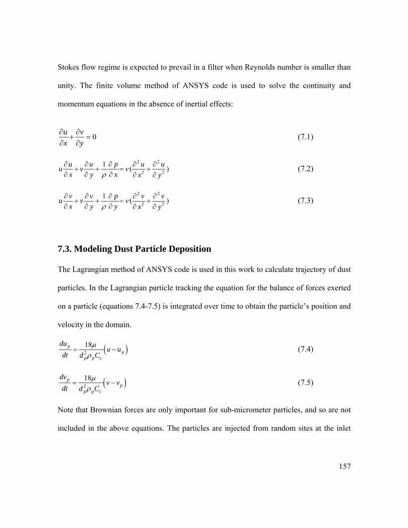
157

Stokes flow regime is expected to prevail in a filter when Reynolds number is smaller than

unity. The finite volume method of ANSYS code is used to solve the continuity and

momentum equations in the absence of inertial effects:

0u vx y∂ ∂

+ =∂ ∂

(7.1)

2 2

2 21 ( )u u p u uu v

x y x x yν

ρ∂ ∂ ∂ ∂ ∂

+ + = +∂ ∂ ∂ ∂ ∂

(7.2)

2 2

2 21 ( )v v p v vu v

x y y x yν

ρ∂ ∂ ∂ ∂ ∂

+ + = +∂ ∂ ∂ ∂ ∂

(7.3)

7.3. Modeling Dust Particle Deposition

The Lagrangian method of ANSYS code is used in this work to calculate trajectory of dust

particles. In the Lagrangian particle tracking the equation for the balance of forces exerted

on a particle (equations 7.4-7.5) is integrated over time to obtain the particle’s position and

velocity in the domain.

( )218p

pp p c

duu u

dt d Cµ

ρ= − (7.4)

( )218p

pp p c

dvv v

dt d Cµ

ρ= − (7.5)

Note that Brownian forces are only important for sub-micrometer particles, and so are not

included in the above equations. The particles are injected from random sites at the inlet

158

boundary because otherwise it leads to formation of unrealistic chain-like particle dendrites

similar to those reported by Payatakes and Tien, (1976).

As mentioned earlier, 3-D microscale simulation of dust loading process in a filter (not a

single fiber) is computationally very expensive. An alternative approach for conducing

such simulations is modeling the filter media in 2-D. However, flow through particle

dendrites is intrinsically three-dimensional, as particles are not 2-D objects. Modeling

particle loading in 2-D geometries lead to unrealistically high pressure drop and collection

efficiencies, as the out of plane component of the velocity field is set to zero in a 2-D

simulation. To overcome this problem, particles (or particle dendrites) can be modeled as

porous particles (or lumped porous deposits) permeable to air but not particles. This

greatly improves the flow field prediction, and consequently reduces the artifacts of a 2-D

model. Nevertheless, one should bear in mind that 2-D simulation of particle loading is

only an approximation.

There a few available studies in which relevant SVF values are reported for dust cakes on a

filter medium (Thomas et al. 2001, Song et al. 2006, Hoffman and Finkers 1995). In our

work, SVF values are obtained from the expression suggested by Kasper et al. (2011) and

assigned to the cells occupied by deposited dust.

0.36 0.44exp( 0.29 )p pdε ρ= + − (7.6)

159

where pd is the particle diameter in micrometer. Note that the porous particles need to be

larger than their solid (impermeable) counterparts. For example, for a cake SVF of 33.3%,

the equivalent porous area will be three times of that of the solid-particle dendrite

( / ( 1 )porous solidp pd d ε= − ). Permeability of the porous area is estimated using the Kozney-

Carman equation (Dullien, 1991).

3 2

2

(1 )180

pKC

dk

αα

−= (7.7)

ANSYS code models a particle as a point mass, and is unable to detect a collision between

a fiber and a particle unless the particle’s center of mass touches the fiber. While this

approximation may be accurate for defining a contact between a particle and a

macroscopically large object, it is not appropriate for calculating particle capture via

interception with a fiber. Similarly, ANSYS’s discrete phase module cannot detect a

collision between a particle and previously deposited particles. To do this, one needs to

record the coordinates of the particles that have already been deposited. When the distance

between a particle and the fiber or the surface of another already deposited particle is

smaller than particle radius, particle velocity should be set equal to zero, i.e., particle

position should be fixed. For modeling a deposited particle, it should be marked as a

porous material so that it can be reused for flow field recalculation and forming particle

dendrite.

160

In our study, two User Defined Memories (UDMs), hereon called UDM0 and UDM1, have

been defined for the ANSYS code to be used in simulating the dendrite structure created

by particle deposition. We start by assigning a zero to the UDM0 value of any

computational cell that does not contain any particle. If the cell becomes filled with a

deposited particle, we then change its UDM0 value to unity. We call this procedure “cell

marking”. Cell marking enables us to distinguish computational cells which contain

deposited particles from the rest. Unlike UDM0, which is a discrete integer of either zero

or one value, UDM1 has a continuous value. UDM1 will be activated when the center of

the deposited particle is in a cell. The area of the cells around the particle’s center of mass

will be added together and stored in UDM1 of that cell until it reaches to equivalent area of

the deposited particle. These cells will be turned into a porous zone with given properties

(equation 7.6). After marking cells containing deposited particles, permeability of the cells

will be changed according to equation (7.7). This procedure is shown in flow chart given in

Figure 7.2. As shown in this flow chart, the distance of a particle from a fiber and any

previously deposited particle is computed in two different loops and compared with the

radius of the particle. As shown in Figure 7.2, the wall domain (i.e., face mesh on the fiber

surface) is picked as the first step. A loop on the face thread (the word thread is used by

ANSYS to refer to a part of a domain or a group of cells) of the wall (i.e., fiber) assigns

coordinates of the faces to a new parameter, which is used to calculate the particle’s

distance from the fiber. If this distance was smaller than one radius, the particle is

considered as deposited. In a second loop, the code searches for marked cells in the flow

cell thread. After finding a marked cell (i.e., where UDM0 is equal to one), the distance of

161

the particle from the cell center is calculated and compared with the particle’s radius. If the

distance is greater than particle radius, it moves through the medium. If the distance is

smaller, the particle is removed from the particle trajectory tracking procedure, and the cell

containing the particle’s center of mass is marked in the UDM0. This procedure continues

until all particles leave the simulation domain or deposit on a fiber or particle. When the

distance of the particle is smaller than the radius, the particle’s center of mass is exported

to a file for further analysis.

A method is developed to capture the circular shape of the particle. Centered on the cell

containing the particle’s center of mass, we consider a circle with a diameter of 0.3 pd , and

grow it to cover as many neighboring cells as needed to make up an area equivalent to that

of the deposited particle. In this process, we allow the circle to grow with an increment of

0.05 pd in radius (see Figure 7.3). Note that this is made possible by considering cells

smaller than the particles. In order to resolve the circular shape of a particle, we first

change the UDM1 value of the cell that contains the particle’s center of mass to the cell’s

area. We then add the areas of the neighboring cells to the area of the specified cell (i.e., its

UDM1) which contained the particle’s center. In this procedure, our UDF searches for

unused cells having a UDM0 value of zero. Thus, we increase the UDM1 value of that cell

by adding the area of the unmarked surrounding cells until it reaches the equivalent area as

the particle. After this procedure is completed, the UDM0 value of the cells associated with

the particle should be changed to one to specify them as porous material. Note that this

162

algorithm enables us to have different particle sizes without needing to re-mesh the

geometry, unlike the work of Kanaoka et al. (1980). With this procedure, one can use a

very fine mesh size to perfectly capture the circular shape of the deposited particles.

In our simulations, the flow field has been recalculated before the total area of deposited

particles reaches 2% of the area of the filter. As we cannot control the number of loaded

particles due to both the random motion and random injection of the particles, this was

controlled instead by limiting the number of particles at injection by trial and error.

7.4. Results and Discussions

To demonstrate capabilities of the numerical scheme developed in this study, we simulated

a series of fibrous filters challenged with dust particles with a diameter of 1 to 5 µm. For

the sake of brevity, we only considered a relevant range of fiber diameters (5 to 15 µm)

and solid volume fractions (2.5 to 7.5%) for the filters simulated.

Figure 7.4 shows examples of particle deposition simulations. The filter shown in Figure

7.4a-d has a fiber diameter of 10µm and an SVF of 2.5% and is exposed to dust particles

with diameters of 1µm, Figure 7.4a and b, and 2µm, Figure 7.4c and d, respectively. The

filter shown in Figure 7.4e-d has a fiber diameter of 10µm and an SVF of 7.5%, and is

exposed to dust particles with a diameter of 5µm. As can be seen in these figures, dust

deposition regime changes quickly from depth filtration (left column), where particles can

penetrate deep into the filter, to surface filtration pattern (right column), in which particles

mostly deposit on the existing particles on the first or second row of the fibers. This

163

transition takes place faster for filters with smaller fiber diameter or higher SVF, when all

other parameters are kept constant. Furthermore, for a given mass of deposited particles,

transition occurs faster when particles are smaller. This is simply because a given mass of

deposit is comprised of more number of small particles than large particles, which in turn

leads to a faster growth of dendrites made up of such particles.

A series of simulations are conducted in this study to produce statistical correlations for

predicting the instantaneous pressure drop and cumulative collection efficiency of fibrous

media under loading condition. The simulation results presented here are repeated at least

two times to improve the statistical errors associated with the randomness of the fibrous

geometries or the particle injection into the domain. The average pressure drop and

collection efficiency values are then used for our correlation development.

To obtain accurate predictions of the instantaneous pressure drop and cumulative

efficiency calculations during the dust load formation, one should update the velocity and

pressure field as frequent as possible by solving the Stokes equations throughout the

domain containing particle deposits. In practice, the number of times one needs to

recalculate the flow field can be obtained by monitoring the effects of flow recalculation

on the pressure drop and collection efficiency. In Figure 7.5, we show how pressure and

cumulative collection efficiency of a filter with a fiber diameter of 5 µm and a solid

volume fraction of 2.5% changes with the frequency of flow recalculation when loaded

with particles having a diameter of 2 µm. As can be seen, the changes in the pressure drop

164

and efficiency predictions become negligible small if the flow field is updated after a mass

of about 2.5µg or less is deposited. Note that this value is only valid for a filter-and-

particle system with dimensions close to those considered in simulations reported in Figure

7.5. For instance, when the dust particles are smaller than 2 µm, it may be necessary

recalculate the flow field more frequently. Therefore, the investigator has to pay close

attention to the rate at which pressure drop and collection efficiency change from one

update to another to ensure an appropriate frequency is adopted. A similar attention should

also be paid to the effects of mesh density on the simulation results. As mentioned earlier,

we used a mesh size of 0.5µm as it was found to be an appropriate optimum size when

considering the trade off between accuracy and CPU time.

7.4.1 Instantaneous Pressure Drop Increase

As mentioned earlier, dust deposition regime changes quickly from depth filtration to

surface filtration. Here we intend to distinguish the two regimes by providing different

expressions for the rate of pressure drop increase in depth and surface filtration regimes.

We normalize the instantaneous pressure drop using the pressure drop of clean media 0p∆ .

In the absence of a better criterion, we assumed transition from depth regime to surface

filtration regime start when the filter’s loaded-to-clean pressure drop ratio increases to a

value of about 3.5. In the depth filtration regime, one can expect that the rate of filter’s

pressure drop increase depends on both the microstructure of the filter and the size of the

particles. On the contrary, in the surface filtration regime, it can be conjectured that the

influence of the filter’s microstructure becomes increasingly less important.

165

Examples of our pressure drop calculations are shown in Figure 7.6 for filters with

different SVFs of 2.5%, 5%, and 7.5%, having two different fiber diameters of 10µm

(Figure 7.6a-b) and 15µm (Figure 7.6c-d). The left column in Figure 7.6, shows the depth

filtration regime while the right column presents both depth and surface filtration regime

(dominated by the surface filtration regime). Here we assumed that the loaded-to-clean

filter pressure ratio varies exponentially with the mass of the deposited particles, and used

Analysis of Variance (ANOVA) to find appropriate exponents β for different filtration

regimes.

0exp( )p M

pβ∆

=∆

(7.8)

Our ANOVA performed for the early stages of the loading process (Figure 7.6a and c)

indicated that, among many other factors, 21 / pd , fd , and α are the most important

parameters influencing the above pressure drop ratio. Therefore, we considered the

following correlation for the exponent β,

10 2 32 f

p

ddλβ λ λ λ α= + + + (7.9)

where pd and fd are in micrometer, and coefficients 0λ , 1λ , 2λ , and 3λ are given in Table

7.1. Similar ANOVA performed for entire loading process, dominated by surface filtration,

(Figure 7.6b and d) indicated that 21 / pd is the most important parameter influencing the

pressure drop ratio. Therefore, we considered

166

10 2

pdωβ ω= + (7.10)

where coefficients 0ω , and 1ω are given in Table 7.2. It is interesting to note that according

to equation (7.10), larger particles lead to smaller β coefficients, indicating slower rate of

pressure drop increase, as expected. As mentioned earlier, for the same mass, smaller

particles form larger dendrite structures causing higher pressure drops. This effect has also

been observed in our previous study conducted for a single fiber (Hosseini and Tafreshi,

2011a).

7.4.2 Instantaneous Cumulative Collection Efficiency

Examples of our cumulative efficiency calculations are shown in Figure 7.7 for the same

filters discussed in section 4.1 (Figure 7.6). Our results reveal that cumulative collection

efficiency does not increase as a linear function as was stated by Kanaoka (1980). As can

be seen, cumulative collection efficiency increases very rapidly in the beginning of loading

process, but it slows down as the dust load grows and surface filtration starts. Our ANOVA

performed for the data shown in Figure 7.7 indicated a large group of parameters

influencing the cumulative collection efficiency of the 27 filters simulated in this study.

Here we developed a correlation for the instantaneous collection efficiency in the

following form.

0E E M δζ= + (7.11)

The ζ and δ parameters that result in the best 2R values have been found to be

167

10 2 3 4 5 6 7 5 8

9 6 0 10 11 5 0 10

1( )( ) ( )( )

1( )( ) ( )( )

p Pf f

f

d dd d

E Ed

ζζ ζ ζ ζ α ζ α ζ ζ ζ α ζ ζ

ζ ζ ζ ζ α ζ ζ

= + + + + + + + + +

+ + + + + + (7.12)

310 2 4 5 6

7 5 8 9 8 6

1( )( )

1 1 1( )( ) ( )( )

p pf f

pf

d dd d

dd

δδδ δ δ δ δ δα

δ δ δ δ δ δα α

= + + + + + +

+ + + + + + (7.13)

The constant coefficients in equation 7.12 and 7.13 are given in Table 7.3 and 7.4,

respectively.

7.5. Modeling Instantaneous Pressure Drop of Pleated Filters

The methodology described in this section can also be modified and used in simulating

dust load deposition on the surface of pleated filter media. To do so, we assume the fibrous

media to be highly efficient like those used in HEPA filters. Such media usually have a

layered microstructure with relatively low permeability. Normally, dust particles (i.e., large

particles with a diameter greater than 2-3 microns) cannot penetrate through such filters.

Consequentially, most of the particles deposit on the surface of the fibrous media leading

to the formation of a surface cake. We performed a series of simulations to model filters

having rectangular (U-shaped) or triangular (V-shaped) pleats with different widths or

angles, respectively.

Spielman and Goren (1968) proposed the following expressions for the in-plane and

through-plane permeability of layered media:

168

1

0

( / )1 1 34 4 4 ( / )

lay layIP IP

layIP

k K r kr K r kα

= + (7.14)

1

0

( / )1 14 2 ( / )

lay layTP TP

layTP

k K r kr K r kα

= + (7.15)

where 0K and 1K are zeroth and first order Bessel functions of the second kind, whereas

layTPk and lay

IPk are permeability constants in the through-plane and in-plane directions,

respectively. In these equations, α is the solid volume fraction of the media and r is the

fiber radius. This information is fed into the Fluent CFD code for simulating the pressure

drop across pleated media. Due to the inherent symmetry of the pleated geometries, we

only considered one pair of pleats bounded by symmetry boundary conditions.

We assumed a constant pleat height of 25.4 mm (1 in.), and the medium thickness of 0.38

mm. For the rectangular and triangular pleats, we considered pleat counts of 3, 4, 5, 7, 10,

15 and 20 pleats per inch and pleat angles of 2, 4, 5, 8, 10, 15 and 20 degrees, respectively.

We also used two inlet velocities of 0.2 m/s and 1.0 m/s, and two dust particle diameters of

3µm and 10µm. To simulate deposition of dust particles, batches of particles were injected

from the inlet over the course of several “time steps”. Aerosol concentration was assumed

to be 132 10× particles per cubic meter. Flow field throughout the domain was recalculated

after deposition of each batch of particles (each time step), and pressure drop was recorded.

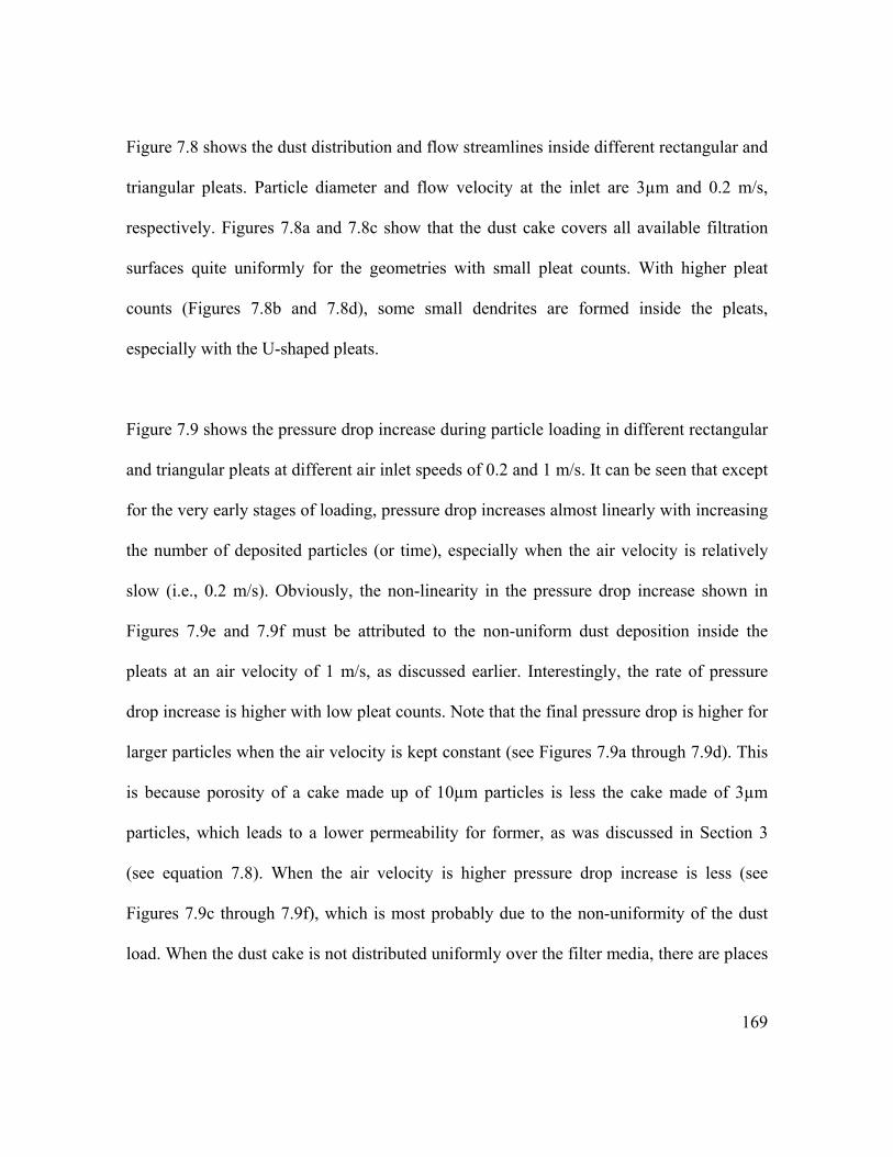
169

Figure 7.8 shows the dust distribution and flow streamlines inside different rectangular and

triangular pleats. Particle diameter and flow velocity at the inlet are 3µm and 0.2 m/s,

respectively. Figures 7.8a and 7.8c show that the dust cake covers all available filtration

surfaces quite uniformly for the geometries with small pleat counts. With higher pleat

counts (Figures 7.8b and 7.8d), some small dendrites are formed inside the pleats,

especially with the U-shaped pleats.

Figure 7.9 shows the pressure drop increase during particle loading in different rectangular

and triangular pleats at different air inlet speeds of 0.2 and 1 m/s. It can be seen that except

for the very early stages of loading, pressure drop increases almost linearly with increasing

the number of deposited particles (or time), especially when the air velocity is relatively

slow (i.e., 0.2 m/s). Obviously, the non-linearity in the pressure drop increase shown in

Figures 7.9e and 7.9f must be attributed to the non-uniform dust deposition inside the

pleats at an air velocity of 1 m/s, as discussed earlier. Interestingly, the rate of pressure

drop increase is higher with low pleat counts. Note that the final pressure drop is higher for

larger particles when the air velocity is kept constant (see Figures 7.9a through 7.9d). This

is because porosity of a cake made up of 10µm particles is less the cake made of 3µm

particles, which leads to a lower permeability for former, as was discussed in Section 3

(see equation 7.8). When the air velocity is higher pressure drop increase is less (see

Figures 7.9c through 7.9f), which is most probably due to the non-uniformity of the dust

load. When the dust cake is not distributed uniformly over the filter media, there are places

170

where cake thickness is very thin or there is no dust at all. This allows air to find the path

of minimum resistance and flow through the filter with minimum pressure drop.

We also compared filters having rectangular and triangular pleats with identical pleat

counts. Here we compare performance of a filter with 15 rectangular pleats per inch with

that of a filter with 15 triangular pleats per inch (pleat angle of 4o). Since both geometries

have the same pleat width, d, hence each injected batch of particles in their corresponding

simulation domains includes the same number of particles. Note that even though both

geometries have the same pleat count, the U-shaped geometry has a slightly more filtration

surface area. The dust distribution and air streamlines inside the above rectangular and

triangular pleats are shown in Figure 7.10 for different air flow velocities of 0.2 and 1 m/s

and different particle diameters of 3 and 10 µm. As can be seen, a uniform dust deposition

covers almost the entire filter surface when the particles are small and the air flow is

relatively slow. As we increase the particle size, non-uniform dendrites begin growing

inside the rectangular pleat (see Figure 7.10b). Eventually, with the large particles and fast

air flow, particles travel deeper inside the channel leaving part of the filtration surface near

the pleat entrance almost clean. This effect is more pronounced with the rectangular pleats.

Results of Figures 7.10 clearly show that dust deposition is more uniform in triangular

pleats.

Figure 7.11 shows pressure drop increase for U-shaped and V-shaped pleats for different

air flow velocities of 0.2 and 1 m/s, and different particle diameters of 3 and 10 µm. These

171

results indicate that a dust-loaded filter with rectangular pleats generate significantly

higher pressure drops when compared to its counterpart having triangular pleats, if the

particles are small and air flow is relatively slow (see Figure 7.11a). As the dust particle

diameter increases from 3µm to 10µm, the difference between the above pressure drop

values starts to vanish (see Figure 7.11b). This is believed to be due to the non-uniform

dust distribution in the rectangular pleats as discussed earlier. Surprisingly, by increasing

the air velocity to 1 m/s, an effect opposite of that shown in Figure 7.11a is observed (see

Figure 7.11c). For the high air velocity of 1m/s and the larger particles (10µm), our

simulations indicate a greater rate of pressure drop increase for the triangular pleats.

7.6. Conclusions

A 2-D approach was considered in this study to simulate the unsteady-state increase of the

pressure drop and cumulative collection efficiency in fibrous media, both at micro- and

macro-scales. Flow field calculations and particle tracking have been performed using the

Fluent CFD code enhanced with in-house C++ subroutines. The additional subroutines

were developed to enable the code to simulate particle deposition on fibers, or previously

deposited particles, and to assign appropriate permeability values to the cells occupied by

the dust cake. A series of microscale simulations has been conducted to demonstrate that

the rate of increase of pressure drop in the depth filtration regime depends on particle

diameter, fiber diameter, and filter porosity, but it becomes almost independent of the

filter’s microstructural parameters when surface filtration regime prevails. Cumulative

172

collection efficiency of the filters has also computed and used to develop an empirical

correlation in terms of filter’s microstructure and particle diameter.

Our macroscale loading simulations were aimed at modeling the effects of dust-load on

pressure drop of pleated filters. Our results indicate that the rate of increase of pressure

drop decreases with increasing the pleat count. We demonstrated that a higher pleat count

results in a higher flow velocity inside the pleat channels causing more non-uniformity in

the dust deposition across the pleat. This effect is observed to be less pronounced when the

pleats have a triangular shape. By comparing filters having 15 pleats per inch, we observed

that rectangular pleats are preferred over the triangular pleats when the particles are highly

inertial, i.e., filtering high-speed large particles.

173

30 fd 5 fd

Inlet

Outlet

Periodic

Figure 7.1- An example of the simulation domains used for the simulations reported in this work together with the boundary conditions. In this case 5fd mµ= , 7.5%SVF = .

174

the particle distance from all fiber

walls are smaller than particleradius

Particle takes another time step

start

particle isin the domain

stop

No

Change the equivalent area as the particle to porous medium

Change the resistivity of marked cells by assigning 1/k

Yes

the particle distance from all marked cells smaller than particle

radius

No

Yes

Yes

No

Add neighboring cells area until UDM1 value reaches the equivalent area

Mark the used cell by changing the value of UDM0 to 1

Figure 7.2- Flow chart of particle loading in medium.

175

(a)

(b)

Figure 7.3- a) Streamlines passing through the loaded particles in medium have shown, b) Particles are captured in flow domain as a collection of cells.

176

2

2.5%pd mµ

α

=

=

c)

2

2.5%pd mµ

α

=

=

d)

5

7.5%pd mµ

α

=

=

e)

5

7.5%pd mµ

α

=

=

f)

1

2.5%pd mµ

α

=

=

a)

depth filtration

1

2.5%pd mµ

α

=

=

b)

surface filtration10fd mµ= 10fd mµ=

Figure 7.4- Loaded dendrites are shown in three different geometries all with 10fd mµ= : a,b) depth & surface filtration ( 1pd mµ= , 2.5%SVF = ), c,d) depth & surface filtration

( 2pd mµ= , 2.5%SVF = ), e,f) depth & surface filtration ( 5pd mµ= , 7.5%SVF = ).

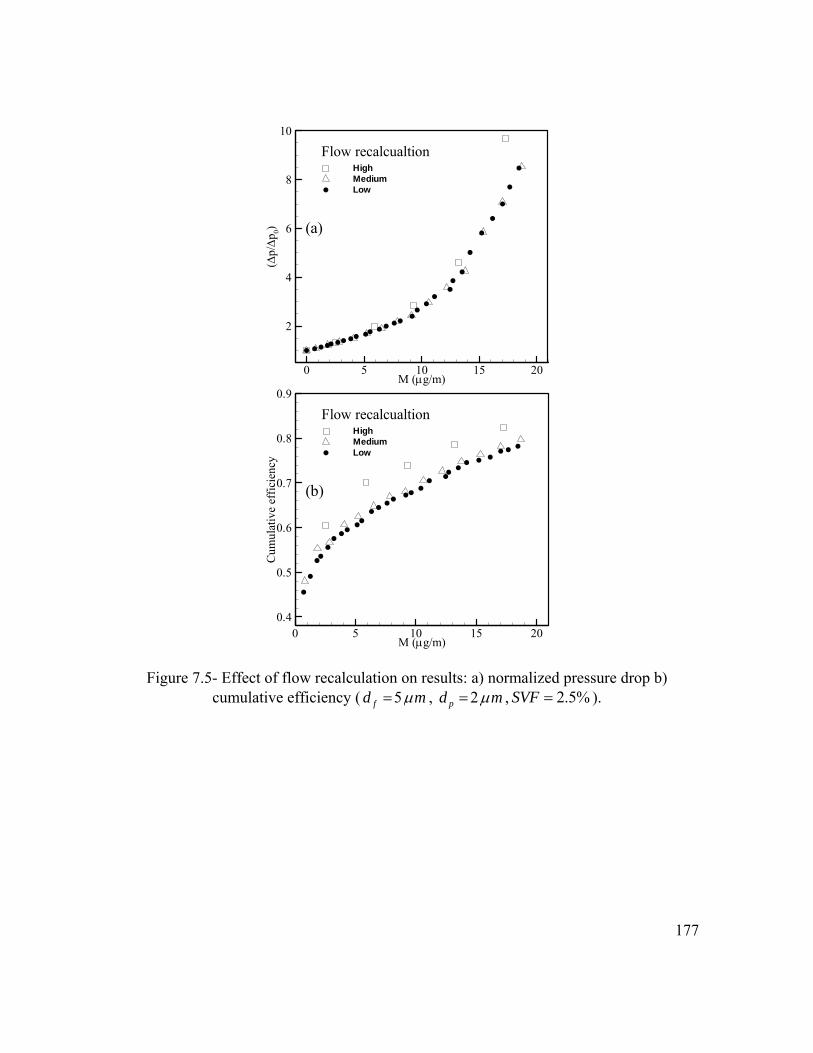
177

M (µg/m)

Cum

ulat

ive

effic

ienc

y

0 5 10 15 200.4

0.5

0.6

0.7

0.8

0.9

HighMediumLow

Flow recalcualtion

M (µg/m)

(∆p/∆p

0)

0 5 10 15 20

2

4

6

8

10

HighMediumLow

Flow recalcualtion

(a)

(b)

Figure 7.5- Effect of flow recalculation on results: a) normalized pressure drop b) cumulative efficiency ( 5fd mµ= , 2pd mµ= , 2.5%SVF = ).

178

M (µg/m)

∆p/∆

p 0

0 5 10

1

2

3

SVF 2.5% (Sim.)SVF 5.0% (Sim.)SVF 7.5% (Sim.)SVF 2.5% (Eq. 9)SVF 5.0% (Eq. 9)SVF 7.5% (Eq. 9)

df=10 µm, dp=2 µm

M (µg/m)

∆p/∆

p 0

0 5 10

1

2

3

SVF 2.5% (Sim.)SVF 5.0% (Sim.)SVF 7.5% (Sim.)SVF 2.5% (Eq. 9)SVF 5.0% (Eq. 9)SVF 7.5% (Eq. 9)

df=15 µm, dp=2 µm

M (µg/m)

∆p/∆

p 0

0 5 10 15 20 25

1

6

11

16

21

SVF 2.5% (Sim.)SVF 5.0% (Sim.)SVF 7.5% (Sim.)(Eq. 10)

df=15 µm, dp=2 µm

M (µg/m)

∆p/∆

p 0

0 5 10 15 20 25

1

6

11

16

21

26

31

SVF 2.5% (Sim.)SVF 5.0% (Sim.)SVF 7.5% (Sim.)(Eq. 10)

df=10 µm, dp=2 µm

(a) (b)

(c) (d)

Figure 7.6- Increasing normalized pressure drop for variable SVFs: a,b) depth & surface filtration compared with equations 7.9 and 7.10 respectively ( 10fd mµ= , 2pd mµ= ), c,d) depth & surface filtration compared with equations 7.9 and 7.10 respectively ( 15fd mµ= ,

2pd mµ= ).

179

M (µg/m)

Cum

ulat

ive

Effic

ienc

y

0 5 10 15 20 250

0.2

0.4

0.6

0.8

1

1.2SVF 2.5% (Sim.)SVF 5.0% (Sim.)SVF 7.5% (Sim.)SVF 2.5% (Eq. 11)SVF 5.0% (Eq. 11)SVF 7.5% (Eq. 11)

df=10 µm, dp=2 µm

M (µg/m)

Cum

ulat

ive

Effic

ienc

y

0 5 10 15 20 25

0

0.2

0.4

0.6

0.8SVF 2.5% (Sim.)SVF 5.0% (Sim.)SVF 7.5% (Sim.)SVF 2.5% (Eq. 11)SVF 5.0% (Eq. 11)SVF 7.5% (Eq. 11)

df=15 µm, dp=2 µm

(a)

(b)

Figure 7.7- Increasing cumulative efficiency for variable SVFs compared with equation 7.11: a) 10fd mµ= , 2pd mµ= , b) 15fd mµ= , 2pd mµ= .

180

a) pleat count =4 plt/in

b) pleat count =20 plt/in

c) pleat count =6 plt/in (2θ =15o)

d) pleat count =15 plt/in (2θ =4o)

Figure 7.8: Dust cake deposition pattern and air streamlines inside rectangular and triangular pleats with a) 4 pleats per inch, b) 20 pleats per inch, c) 15o pleat angle, and d) 4o

pleat angle. Particle diameter and flow velocity are 3µm and 0.2 m/s, respectively.

181

- - - - - --

- - - - - - - - - - - - - - - - - - - - - - - - - - - - - - - - - -

+ + + + + + + + + + + + + + + + + + + + + + + + + + + + + + + + + + + + + + + + +

Number of time steps

∆p/∆

p 0

0 50 100 150

2

4

6

8 15o pleat angle10o pleat angle8o pleat angle5o pleat angle4o pleat angle3o pleat angle

-

+

V-shapeddp= 3 µm

b)

uin=0.2 m/s

- - - - --

- - - - - - - - - - - - - - - - - - - - - - - - - - - - - - - - - - -

+ + + + + + + + + + + + + + + + + + + + + + + + + + + + + + + + + + + + + + + + +


∆p/∆

p 0

0 50 100 1500

10

20 4 pleat/in5 pleat/in7 pleat/in10 pleat/in15 pleat/in20 pleat/in

-

+

U-shapeddp= 3 µm

a)

uin=0.2 m/s

- - - - - - - - - - - - - - - - - - - - - - - - - - - - - - - - - - - - - -- -

-

+ + + + + + + + + + + + + + + + + + + + + + + + + + + + + + + + + + + + + + + + +


∆p/∆

p 0

0 50 100 1500

10

20


-

+

U-shapeddp= 10 µm

c)

uin=0.2 m/s

- - - - - - -- - - - - - - - - - - - - - - - - - - - - - - - - - - - - - - - - -

+ + + + + + + + + + + + + + + + + + + + + + + + + + + + + + + + + + + + + + + + +


∆p/∆

p 0

0 50 100 1500

5

10

15o pleat angle10o pleat angle8o pleat angle5o pleat angle4o pleat angle3o pleat angle

-

+

V-shapeddp= 10 µm

d)

uin=0.2 m/s

- - - - - - - - - - - - - - - - - - - - - - - - - - - - - - - - - - - - - - - - -

+ + + + + + + + + + + + + + + + + + + + + + + + + + + + + + + + + + + + + + + + +


∆p/∆

p 0

0 50 100 150

2

4

6


-

+

U-shapeddp= 10 µm

e)

uin=0.2 m/s

- - - - - --

--

--

- -- - - - - - - - - - - - - - - - - - - - - - - - - - - -

+ + + + + + + + + + + + + + + + + + + + + + + + + + + + + + + + + + + + + + + + +


∆p/∆

p 0

0 50 100 150

1

2

3

15o pleat angle10o pleat angle8o pleat angle5o pleat angle4o pleat angle3o pleat angle

-

+

V-shapeddp= 10 µm

f)

uin=0.2 m/s

Figure 7.9: Pressure drop increase during particle loading with rectangular and triangular pleats for particles with diameters of 3 and 10µm and air inlet velocities of 0.2 and 1m/s.

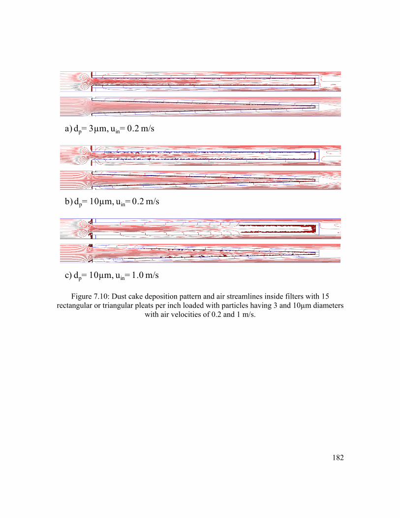
182

b) dp= 10µm, uin= 0.2 m/s

c) dp= 10µm, uin= 1.0 m/s

a) dp= 3µm, uin= 0.2 m/s

Figure 7.10: Dust cake deposition pattern and air streamlines inside filters with 15 rectangular or triangular pleats per inch loaded with particles having 3 and 10µm diameters

with air velocities of 0.2 and 1 m/s.

183


∆p/∆

p 0

0 50 100 1501

2

3

4

5U-shaped, 15 pleat/inV-shaped, 4o pleat angle

dp= 3 µmuin= 0.2 m/s

a)


∆p/∆

p 0

0 50 100 1501

2

3

4

5U-shaped, 15 pleat/inV-shaped, 4o pleat angle


b)


∆p/∆

p 0

0 50 100 150

1

1.2

1.4

1.6 U-shaped, 15 pleat/inV-shaped, 4o pleat angle


c)

Figure 7.11: Comparison between the pressure drop increase for filters with 15 rectangular and triangular pleats per inch loaded with particles having 3 and 10µm diameters with air

velocities of 0.2 and 1 m/s.

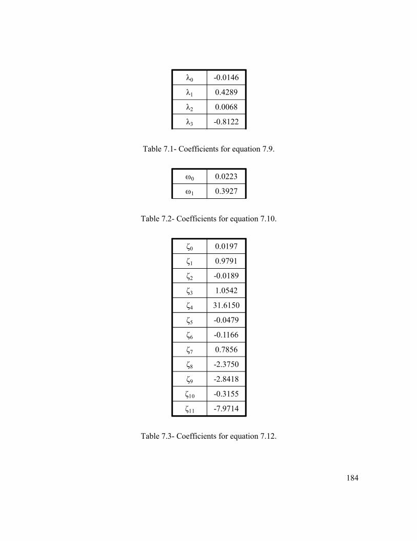
184

λ0 -0.0146

λ1 0.4289

λ2 0.0068

λ3 -0.8122

Table 7.1- Coefficients for equation 7.9.

ω0 0.0223

ω1 0.3927


ζ0 0.0197

ζ1 0.9791

ζ2 -0.0189

ζ3 1.0542

ζ4 31.6150

ζ5 -0.0479

ζ6 -0.1166

ζ7 0.7856

ζ8 -2.3750

ζ9 -2.8418

ζ10 -0.3155

ζ11 -7.9714


185

δ0 0.7893

δ1 -2.5626

δ2 -0.0748

δ3 0.0061

δ4 -0.6058

δ5 -0.1166

δ6 -2.3750

δ7 0.0442

δ8 -25.5555

δ9 0.0049


186

CHAPTER 8. Overall Conclusion

Over the past decades, numerous analytical and/or numerical expressions have been

developed for predicting the permeability of a fibrous medium. These expressions,

however, are not accurate in predicting the permeability of media that operate in the slip

flow regime––nanofiber media. Generating a large series of 3-D virtual geometries that

resemble the microstructure of a nanofiber filter medium, the influence of fiber diameter

and Solid Volume Fraction (SVF) on the media’s permeability is studied here, and used to

establish a correction factor for the existing permeability expressions when used for

nanofiber media (see equation 2.16). These virtual 3-D geometries are also used to predict

collection efficiency of nanofibrous media when challenged with aerosol particles in the

size range of 25 to 1000 nanometers (see Chapter 3). Particle collection efficiency of the

above fibrous media are calculated and compared with the analytical/empirical results from

the literature. The numerical simulations conducted in this work are believed to be the

most complete and realistic filter modeling published to date. Our simulation technique,

unlike previous studies based on oversimplified 2-D geometries, do not need any empirical

correction factors, and can be used to directly simulate efficiency of any fibrous media.

The effects of fibers’ cross-sectional shape on the performance of fibrous filters in the slip

and no-slip flow regimes is investigated to conclude that while collection efficiency is only

weakly affected by the cross-sectional shape of nanofibers, the fiber drag (i.e., permeability

of the media) can be considerably influenced by the fiber’s shape (see Chapter 5).

187

Simulating flow field around nano- and microfibers with circular, square, trilobal, and

elliptical cross-sections, it was found that, the more streamlined the fiber geometry, the

lower the fiber drag caused by a nanofiber relative to that generated by its micron-sized

counterpart.

In Chapter 4, results of a series of simulations conducted in 2-D disordered geometries

comprised of randomly distributed fibers are discussed in comparison with our 3-D

simulations and those obtained from the existing cell-model-type (ordered 2-D models)

semi-analytical correlations. Our results revealed that disordered 2-D fiber arrangements

can be utilized to predict performance of fibrous filters with reasonable accuracy and CPU

time. Collection efficiencies obtained from our 2-D models seem to be marginally lower

than those of 3-D simulations, for nanoparticles, and slightly higher, for larger particles.

Pressure drop predictions of disordered 2-D media are found to be lower than that of

ordered 2-D models, but higher than that of 3-D fibrous models. The later is found to be in

very good agreement with experiment.

In Chapter 6, a methodology is presented for simulating pressure drop and collection

efficiency of a filter medium during instantaneous particle loading using the Fluent CFD

code enhanced using in-house subroutines. A series of in-house subroutines are developed,

and described in detail which allow one to track particles of different sizes and simulate

formation of 3-D dendrite particle deposits. The deposition of particles on a fiber and the

188

previously deposited particles is made possible by developing two additional subroutines,

which mark the cells located at the deposition sites and modify their properties to so that

they resemble solid particles. Fiber drag and single fiber collection efficiencies are

obtained from simulations for fibers and particles of different diameters for demonstration

purposes. Effects of particle capture mechanisms on a filter’s pressure drop and collection

efficiency are presented and discussed with respect to the studies reported in the literature.

More specifically, two fiber diameters of 1 and 20µm are used to demonstrate that the

normalized single fiber collection efficiency increases with increasing mass of the loaded

particles on the fibers (i.e., time) if the particle capture mechanism is interception or

diffusion, but stays almost invariant if the capture mechanism is inertial impaction. Fiber

drag (resembling the filter’s pressure drop) seems to increase because of particle deposition

but with different rates for different particle capture regimes.

In Chapter 7, a 2-D approach was developed to simulate the unsteady-state increase of the

pressure drop and cumulative collection efficiency in fibrous media, both at micro- and

macro-scales. Our microscale simulations demonstrated that the rate of increase of pressure

drop in the depth filtration regime depends on particle diameter, fiber diameter, and filter

porosity, but it becomes almost independent of the filter’s microstructural parameters when

surface filtration regime prevails. Our macroscale loading simulations were aimed at

modeling the effects of dust-load on pressure drop of pleated filters. These results indicated

that the rate of increase of pressure drop decreases with increasing the pleat count. We

demonstrated that a higher pleat count results in a higher flow velocity inside the pleat

189

channels causing more non-uniformity in the dust deposition across the pleat. Comparing

filters having 15 pleats per inch, we observed that rectangular pleats are preferred over the

triangular pleats when the particles are highly inertial, i.e., filtering high-speed large

particles.

190

List of References

Barber, R.W., Emerson, D.R., 2002. The Influence of Knudsen Number on the Hydrodynamic Development Length within Parallel Plate Micro-channels. Advances in Fluid Mechanics IV, pp. 207-216. Box, G. E. P., Muller, M.E., 1958. A Note on the Generation of Random Normal Deviates, The Annals of Mathematical Statistics 29 (2), 610–611. Brown, R.C., 1993. Air Filtration. Pergamon Press. Brown, R.C., 1984. Many-fiber model of airflow through a fibrous filter. Journal of Aerosol Science 15 (1984) 583-593. R.C. Brown, Thorpe, A., 2001. Glass-fiber filters with bimodal fiber size distributions, Powder Technology 118, 3-9. Chen, X., Papathanasiou, T.D., 2006. On The Variability of the Kozeny Constant For Saturated Flow Across Unidirectional Disordered Fiber Array. Composite Part A 37, 836-834. Cheung, C.S., Cao, Y.H., Yan, Z.D., 2005. Numerical model for particle deposition and loading in electret filter with rectangular split-type fibers. Computational Mechanics 35(6), 449-458. Clague, D.S., Phillips, R.J., 1997. A Numerical Calculation of the Hydraulic Permeability of Three-Dimensional Disordered Fibrous Media. Physics of Fluids 9, 1562. Clague, D.S., Kandhai, D.B., Zhang, R., 2000. Hydraulic Permeability of (Un)bounded Fibrous Media Using Lattice Boltzmann Method. Physical Review E 61(1), 616-625. Davies, C.N. ,1973. Air Filtration. Academic Press, London. Dhaniyala, S., Liu, B.Y.H., 1999. An Asymmetrical, Three-Dimensional Model for Fibrous Filters. Aerosol Science and Technology 30 (4), 333-348. Drummond, J.E., Tahir, M.I., 1984. Laminar viscous flow through regular arrays of parallel solid cylinders. International Journal of Multiphase Flow 10, 515-540. Duggirala, K.R., Roy, J.C., Saeidi, M.S., Khodadadi, M.J., Cahela, R.D., Tatarchuk, J.B., 2008. Pressure Drop Prediction in Micro-Fibrous Materials Using Computational Fluid Dynamics. ASME Journal of Fluid Engineering (130), 071302-1 to 071302-13.

191

Dullien, F.A.L., 1991. Porous Media, Fluid Transport and Pore Structure. Academic Press Inc. 2nd edition. Dunnett, S.J., Clement C.F., 2009. A numerical model of fibrous filters containing deposit. Eng Analysis Boundary Elements 33(5), 601-610. Filippova, O., Hanel, D., 1997. Lattice-Boltzmann simulation of gas-particle flow in filters. Computers & Fluids 26(7), 697-712. Fotovati, S., Tafreshi, H.V., Ashari, A., Hosseini, S.A., Pourdeyhimi, B., 2010. Analytical Expressions for Predicting Capture Efficiency of Bimodal Fibrous Filters, Journal of Aerosol Science 41, 295. Fotovati, S., Tafreshi, H.V., Pourdeyhimi, B., 2011a. Analytical expressions for predicting performance of aerosol filtration media made up of trilobal fibers, Journal of Hazardous Materials 186(2-3), 1503-1512. Fotovati, S., Hosseini, S.A., Tafreshi, H.V., and Pourdeyhimi, B., 2011b. Modeling Instantaneous Pressure Drop of Pleated Thin Filter Media during Dust Loading”, Chemical Engineering Science, in press. Friedlander, S.K., 2000. Smoke, Dust, and Haze: Fundamentals of Aerosol Dynamics, 2nd edition Oxford University Press. Happel, J., 1959. Viscous flow relative to arrays of cylinders, AIChE Journal 5(2) 174-177. Hosseini, S.A., Tafreshi, H.V., 2010a. Modeling Permeability of 3-D Nanofiber Media in slip flow regime. Chemical Engineering Science 65, 2249- 2254. Hosseini, S.A., Tafreshi, H.V., 2010b. 3-D Simulation of Particle Filtration in Electrospun Nanofibrous Filters. Powder Technology 201, 153-160. Hosseini, S.A., Tafreshi, H.V., 2010c. Modeling particle filtration in disordered 2-D domains: A comparison with cell models. Separation and Purification Technology 74, 160–169. Hosseini, S.A., Tafreshi, H.V., 2011a. On the Importance of Fibers’ Cross-Sectional Shape for Air Filters Operating in the Slip Flow Regime. Powder Technology, 212 (3), 425-431 (2011).. Hosseini, S.A., Tafreshi, H.V., 2011b. Modeling Particle-Loaded Single Fiber Efficiency and Fiber Drag using Fluent CFD Code. Under review in Computers and Fluids.

192

Hosseini, S.A., Tafreshi, H.V., 2011c. Microscale 2-D Modeling of Instantaneous Dust Loading of Fibrous Filters, To be submitted. Henry, F. S., Ariman, T., 1983. Particulate Science & Technology 1, 1-20. Higdon, J.J.L., Ford, G.D., 1996. Permeability of Three-Dimensional Models of Fibrous Porous Media, Journal of Fluid Mechanics 308, 341-361. Hinds, W.C., 1999. Aerosol technology: properties, behavior, and measurement of airborne particles, 2nd edn, Wiley, New York. Hoffmann, A.C., Finkers, H.J., 1995. A relation for the void fraction of randomly packed particle Beds, Powder Technology, 82, 197-203. Jackson , G., James, D., 1986. The Permeability of Fibrous Porous Media. The Canadian Journal of Chemical Engineering 64, 364. Jaganathan, S., Tafreshi, H.V., Pourdeyhimi, B., 2008a. A Realistic Approach for Modeling Permeability of Fibrous Media: 3-D Imaging Coupled with CFD Simulation. Chemical Engineering Science 63, 244. Jaganathan, S., Tafreshi, H.V., Pourdeyhimi, B., 2008b. A Case Study of Realistic Two-Scale Modeling of Water Permeability in Fibrous Media, Separation Science& Technology 43, 1901. Jaganathan, S., Tafreshi, H.V., Pourdeyhimi, B., 2008c. On the Pressure Drop Prediction of Filter Media with Bimodal Fiber Diameter. Powder Technology 181, 89. Kanaoka, C., Emi, H., Myojo, T., 1980. Simulation of the growing process of a particle dendrite and evaluation of a single fibre collection efficiency with dust load. Journal of Aerosol Science 11, 377–389. Kanaoka, C., Hiragi, S., Tanthapanichakoon, W., 2001. Stochastic simulation of the agglomerative deposition process of aerosol particles on an electret fiber. Powder Technology 118, 97-106. Karadimos, A., Raffaella, O., 2003. The effect of the flow field recalculation on fibrous filter loading: a numerical simulation. Powder Technology 137, 109- 119. Kasper, G., Schollmeier, 1., Meyer, J., Hoferer, J., 2009. The collection efficiency of a particle-loaded single filter fiber. Journal of Aerosol Science 40, 993–1009.

193

Kasper, G., Schollmeier, S., Meyer, J., 2010. Structure and density of deposits formed on filter fibers by inertial particle deposition and bounce. Journal of Aerosol Science 41(12), 1167-1182. Kirsh, V.A., 2003. Deposition of aerosol nanoparticles in fibrous filters, Colloid Journal 65(6), 726-732. Kuwabara, S., 1959. The Forces Experienced by Randomly Distributed Parallel Circular Cylinders of Spheres in a Viscous Flow at Small Reynolds Number. Journal of the Physical Society of Japan 14 (4), 527-532. Lamb, G.E.R., Costanza, P.A., 1980. Influences of Fiber Geometry on the Performance of Non-Woven Air Filters: 3. Cross-Sectional Shape, Textile Res. Journal 50 (6), 362-370. Lantermann, U., Hanel, D., 2007. Particle Monte Carlo and lattice-Boltzmann methods for simulations of gas-particle flows. Computers Fluids 36(2), 407-422. Lehmann, M. J., Hardy, E.H., Meyer, J., Kasper, G., 2005. Fibrous Filters: Non-Invasive Determination of Local 3D Fiber Structure by MRI. Filtration 5(2), 62-67. Lee, K.W. , Liu, B.Y.H., 1982. Theoretical study of aerosol filtration by fibrous filters, Aerosol Sci. Technol 1, 147-161. Lee, K.W., Gieseke, J.A., 1980. Note on the approximation of interceptional collection efficiencies J. Aerosol Sci. 11, 335-341. Li, S.Q., Marshall, J.S., 2007. Discrete element simulation of micro-particle deposition on a cylindrical fiber in an array. Journal of Aerosol Science 38(10), 1031-1046. Li, Y., Park, C., 1997. Deposition of Brownian particles on cylindrical collectors in a periodic array, Journal of Colloid and Interface Science 185 (1), 49. Li, A., Ahmadi, G., 1992. Dispersion and deposition of spherical-particles from point sources in a turbulent chemical flow, Aerosol Sci. Tech. 16, 209-226. Liu, B.Y.H., Rubow, K.L., 1990. Efficiency, pressure drop and figure of merit of high efficiency fibrous and membrane filter media, in: Proceedings of the Fifth world filtration congress, Nice. Longest, P.W., Jinxiang, X., 2007. Effectiveness of Direct Lagrangian Tracking Models for Simulating Nanoparticle Deposition in the Upper Airways. Aerosol Science and Technology, 41, 380–397.

194

Mattern, K.J., Deen, W.M., 2007. “Mixing Rules” for Estimating the Hydraulic Permeability of Fiber Mixtures. AIChE Journal 54(1), 32-41. Maze, B., Tafreshi, H.V., Wang, Q., Pourdeyhimi, B., 2007. Unsteady-State Simulation of Nanoparticle Aerosol Filtration via Nanofiber Electrospun Filters at Reduced Pressures. Journal of Aerosol Science, 38, 550 . McNenly, J.M., Gallis A.M., Boyd D.I., 2005. Empirical Slip and Viscosity Model Performance for Micro-Scale Gas Flow. International Journal for Numerical Method in Fluids (49), pp. 1169-1191. Myojo, T., Kanaoka, C., Emi, H., 1984. Experimental observation of collection efficiency of a dust-loaded fiber. Journal of Aerosol Science 15, 483- 489. Ogorodnikov, B.I., 1976. Pressure-Drop Across FP Fiber Filters Under Gas Slip-Flow and in Transition Regime. Colloid Journal of the USSR, 38, 1, 168-172. Payatakes, A.C., Tien, C., 1976. Particle deposition in fibrous media with dendrite-like pattern: A preliminary model. Journal of Aerosol Science 7, 85-100. Payatakes, A.C., Gradon, L., 1980. Dendritic Deposition of aerosols by convective Brownian diffusion for small, intermediate and high particle Knudsen numbers. AICHE Journal 26 (3), 443-454. Payet, S., 1991. Filtration stationnaire et dynamique des aerosols liquids submicroniques, These de l’universite Paris ХІІ4 oct. 150 p., rapport CEA-R-5589. Patankar, S.V., 1980. Numerical Heat Transfer and Fluid Flow, Hemisphere Pub. Washington. Pich, J., 1965. The filtration theory of highly dispersed aerosols. Staub Reinhalt. Luft, 5, 16-23 (in English). Pich, J., 1966. The effectiveness of the barrier effect in fiber filters at small Knudsen numbers, Staub Reinhalt. Luft. 26, 1-4. Podgorski, A., Balazy, A., Gradon, L., 2006. Application of nanofibers to improve the filtration efficiency of the most penetrating aerosol particles in fibrous filters. Chemical Engineering Science 61 (20), 6804-6815. Przekop, R., Moskal, A., Gradon, L., 2003. Lattice-Boltzmann approach for description of the structure of deposited particulate matter in fibrous filters. Journal of Aerosol Science 34(2), 133-147.

195

Przekop, R., Gradon, L., 2008. Deposition and filtration of nanoparticles in the composites of nano- and microsized fibers. Aerosol Science and Technology 42 (6), 483-493. Ramarao, B.V., Tien, Chi , Mohan, S., 1994. Calculation of single fiber efficiencies for interception and impaction with superposed Brownian motion, Journal of Aerosol Science 25 (2), 295-313. Rao, N., Faghri, M., 1988. Computer modeling of aerosol filtration by fibrous filters, Aerosol Science and Technology 8 (2), 133-56. Raynor, P.C., 2008. Single-fiber interception efficiency for elliptical fibers. Aerosol Science and Technology 42, 357-368. Rodman, C.A., Lessmann, R.C., 1988. Automotive Nonwoven Filter Media: Their Constructions and Filter Mechanism. Tappi Journal 71, 161-168. Sanchez, J.R., Rodriguez, J.M., Alvaro, A., Estevez, A.M., 2007. The capture of fly ash particles using circular and noncircular cross-section fabric filters, Environ. Prog. 26 (1) 50-58. Shin, C., Chase, G.G., 2004. Water-in-oil coalescence in micro-nanofiber composite filters, AICHE Journal 50 (2), 343-350. Song, C.B., Park, H.S., Lee, K.W., 2006. Experimental study of filter clogging with monodisperse PSL particles. Powder Technology 163, 152–159. Spielman , L., Goren, S.L., 1968. Model for Predicting Pressure Drop and Filtration Efficiency in Fibrous Media. Environmental Science and Technology 2, 279. Spurny, K.R., 1998. Advanced aerosol filtration, Lewis publishers. Stechkina, I.B., Fuchs, N.A., 1965. Studies on fibrous aerosol filters-I. Calculation of diffusional deposition of aerosols in fibrous filters. Annual of Occupational Hygiene 9, 59-64. Stechkina, I.B., 1966. Diffusion precipitation of aerosols in fiber filters, Dokl. Acad. Nauk. SSSR 167, 1327. Steffens, J., Coury, J.R., 2007. Collection efficiency of fiber filters operating on the removal of nano-sized aerosol particles - II. Heterogeneous fibers. Separation Purification Technology 58(1), 106-112.

196

Stone, H.A., Strook, A.D., Ajdari, A., 2004. Engineering Flows in Small Devices: Micro Fluidics toward a Lab-on-a-chip. Ann. Rev. Fluid Mechanics (36), pp. 381-411. Tafreshi , H.V., Rahman, M.S., Jaganathan, S., Wang, Q., Pourdeyhimi, B, 2009. Analytical Expressions for Predicting Permeability of Bimodal Fibrous Porous Media. Chemical Engineering Science 64:6, 1154-1159. Tahir, M.A., Tafreshi, H.V., 2009. A Study on the Influence of Fiber Orientation on the In-Plane Permeability of Fibrous Media, Physics of Fluids 21, 083604. Tomadakis, M.M., Robertson, J. T., 2005.Viscous Permeability of Random Fiber Structures: Comparison of Electrical and Diffusional Estimates with Experimental and Analytical results. Journal of Composite Materials 39(2), 163-188. Thomas, D., Penicot, P., Contal, P., Leclerc, D., Vendel, J., 2001. Clogging of fibrous filters by solid aerosol particles experimental and modeling study, Chemical Engineering Science 56, 3549–3561. Wang, Q., Maze, B., Tafreshi, H.V., Pourdeyhimi, B., 2006a. A Note on Permeability Simulation of Multifilament Woven Fabrics. Chemical Engineering Science 61, 8085. Wang , Q., Maze, B., Tafreshi, H.V., Pourdeyhimi, B., 2006b. A Case Study of Simulating Submicron Aerosol Filtration via Spun-bonded Filter Media. Chemical Engineering Science 61, 4871. Wang, Q., Maze, B., Tafreshi, H.V., Pourdeyhimi, B., 2007. Simulating Through-plane Permeability of Fibrous Materials Having Different Fiber Lengths. Modeling & Simulation in Materials Science and Engineering, 15, 855-868. Wang, J., Kim, S.C., Pui, D.Y., 2008. Investigation of the figure of merit for filters with a single nanofiber layer on a substrate, Journal of Aerosol Science 39 (4), 323-334. Wang, J., Pui, D.Y.H., 2009. Filtration of aerosol particles by elliptical fibers: a numerical study, J. Nanopart. Res. 11, 185-196. Zhao, S., Povitsky, A., 2009. Method of fundamental solutions for partial-slip fibrous filtration flows, International Journal For Numerical Methods in Fluids, 61 (3), 255-274. Zhu, C., Lin, C.H., Cheung, C.S., 2000. Inertial impaction-dominated fibrous filtration with rectangular or cylindrical fibers, Powder Technology 112(1-2), 149-162.

197

Zobel, S., Maze, B., Tafreshi, H.V., Wang, Q., Pourdeyhimi, B., 2007. Simulating Permeability of 3-D Calendered Fibrous Structures. Chemical Engineering Science 62, 6285.

198

Seyed Alireza Hosseini Home address: 244 Donna Avenue Morgantown, WV 26505 Tel: 804-677-0430

Email: [email protected]

Education:

Ph.D. Candidate, Mechanical Engineering Aug. 2011 Virginia Commonwealth University, Virginia (GPA: 4.0 out of 4.0)

Dissertation: Modeling Particle Filtration and Caking in Fibrous Filter Media

M.Sc., Mechanical Engineering 2008 Sharif University of Technology, Tehran, Iran (GPA: 16.42 out of 20) Dissertation: Numerical Modeling of Oil Reservoir

B.Sc., Mechanical Engineering (Fluid Mechanics) 2005 University of Tehran, Tehran, Iran (GPA: 16.16 out of 20) Dissertation: Modeling Slip Flow and Heat Transfer in Microchannels

Journal Publications:

• S.A. Hosseini and H.V. Tafreshi, Microscale 2-D Modeling of Instantaneous Dust Loading of Fibrous Filters (To be submitted)

• S.A. Hosseini and H.V. Tafreshi, Modeling Particle-Loaded Single Fiber Efficiency and

Fiber Drag using Fluent CFD Code (Under review). • S. Fotovati, S.A. Hosseini, and H.V. Tafreshi. Modeling Instantaneous Pressure Drop of

Pleated Thin Filter Media During Dust Loading, Chemical Engineering Science 66, 4036-4046 (2011).

• S.A. Hosseini and H.V. Tafreshi, On the Importance of Fibers’ Cross-Sectional Shape for

Air Filters Operating in the Slip Flow Regime, Powder Technology 212 (3), 425-431 (2011).

• R. Arambakam, S.A. Hosseini, H.V. Tafreshi, and B. Pourdeyhimi. A Monte Carlo

Simulation of Radiative Heat through Fibrous Media: Effects of Boundary Conditions and Microstructural Parameters, International Journal of Thermal Sciences 50(6), 935-941 (2011).

• M.A. Tahir, H.V. Tafreshi, S.A. Hosseini, and B. Pourdeyhimi, Modeling the Role of

Microstructural Parameters in Radiative Heat Transfer through Disordered Fibrous Media,

199

International Journal of Heat & Mass Transfer 53, 4629-4637 (2010). • S.A. Hosseini and H.V. Tafreshi, Modeling Particle Filtration in Disordered 2-D Domains:

A Comparison with Cell Models, Separation and Purification Technology 74, 160-169 (2010).

• S.A. Hosseini and H.V. Tafreshi, 3-D Simulation of Particle Filtration in Electrospun

Nanofibrous Filters, Powder Technology 201, 153-160 (2010). • S.A. Hosseini and H.V. Tafreshi, Modeling Permeability of 3-D Nanofiber Media: Effects

of Slip Flow, Chemical Engineering Science 65, 2249 (2010). • S. Fotovati, H.V. Tafreshi, A. Ashari, S.A. Hosseini, and B. Pourdeyhimi, Analytical

Expressions for Predicting Capture Efficiency of Bimodal Fibrous Filters, Journal of Aerosol Science 41, 295 (2010).

Selected Conference Proceedings:

• S.A. Hosseini and H.V. Tafreshi, On the Drag Force and Collection Efficiency of Circular and Non-Circular, Clean and Loaded Submicron Fibers, American Filtration & Separation (AFS) Annual Conference, May 9-12 (2011), Louisville, KY.

• S.A. Hosseini and H.V. Tafreshi, Transient Modeling Filtration Efficiency of Nanofiber

Filters: 3-D Domains vs. 2-D Domains, American Filtration & Separation (AFS) Annual Conference, May 9-12 (2011), Louisville, KY.

• S.A. Hosseini and H.V. Tafreshi, Modeling filtration efficiency of Electrospun

Nanofibrous filters, Nanofibers for the 3rd Millennium, August 30- September 1 (2010), Raleigh, NC.

• S.A. Hosseini and H.V. Tafreshi, Modeling Particle Loading in Fibrous Filter Media,

American Filtration & Separation (AFS) Annual Conference, March 22-25 (2010), San Antonio, TX.

• S.A. Hosseini and H.V. Tafreshi, Modeling Particle Filtration in 3-D Electrospun

Nanofibrous Filters, , American Filtration & Separation (AFS) Annual Conference, March 22-25 (2010), San Antonio, TX.

• S.A. Hosseini and H.V. Tafreshi, Three-dimensional Simulation of Particle Filtration in

Electrospun Nanofibrous Filters, American Filtration & Separation (AFS) Annual Conference, May 4-7 (2009), Minneapolis, MN.

200

Computational Skills:

• Experienced with CFD packages like Fluent (User Defined Functions), Gambit, GeoDict • Proficient programming skills in C++, Fortran, MATLAB, QuickBASIC • Experienced with PDMS (Petrochemical Piping Design Software), Ceazar II(Stress

Analysis) • Experienced with SolidWorks, AutoCAD, Tecplot • Familiar with ANSYS, DASYLab, statistical software R, JMP and Festo Pneumatic

software

Honors and Awards:

• Selected and honored as the Best Graduate Student of Engineering School at VCU, 2010-2011.

• Graduate Fellowship from the National Science Foundation, 2010. • Ranked 13th among approximately 10,000 participants in the national wide entrance

examination held in Iran every year for admission into M.Sc. degree of Mechanical Engineering, 2005.

• Highest GPA among students at University of Tehran, 2003. • Ranked 210 among approximately 600,000 participants in the national wide entrance

examination held in Iran every year for admission into the universities, 2000. • The only person in Iran who passed the first level of the four Olympiad exams in

Mathematics, Computer, Physics, and chemistry, 1999. •

Employment History:

• Modeling Air Filtration in Fibrous Filters (Jan. 2009- Jun. 2011) Porous Media & Multiphase Flow Laboratory, Richmond, VA (www.vcu.edu) o Developed different models for predicting clean and loaded filter performance o Optimized pleated filters by studying unsteady state particle loading o Developed user defined functions (UDFs) and C++ codes to model filter media

• Piping Design Engineer and Piping Supervisor (Jan. 2008- Dec. 2008)

Sazeh Consultants, Tehran, Iran (www.sazeh.com) o Routed piping of about 400 lines in PDMS, and Autoplant, added piping supports o Good exposure to piping stress analysis (using CAESAR II) o Prepared piping plans, isometrics, MTO, Technical specification

201

• Compilation of IPS (Iranian Petroleum Standards) (Dec. 2006- Dec. 2007) National Iranian Oil Refining & Distribution Company, Tehran, Iran

(www.en.niordc.ir) o Updated Iranian Petroleum Standard based on requested questions

• Lecturer (Jul. 2006- Dec. 2008)

Payame Noor University, Tehran, Iran (www. en.pnu.ac.ir) Islamic Azad University, Tehran, Iran (www.iau.ac.ir/indexen.htm) o As a lecturer, taught different mechanical engineering courses in undergraduate level such

as Engineering Mathematics, Heat Transfer, Fluid Mechanics, Thermodynamics, and Static at IAU, PNU, and VCU.

o Teaching Assistant of Engineering Mathematics and Heat Transfer courses in undergraduate level during PhD education for duration of one semester at VCU.

• Design Engineer using SolidWorks (Jul. 2006- Dec. 2006)

EIED (Energy, Industries, Engineering and Design), Tehran, Iran (www.eied.com) o Designed automated parts and assembly using SolidWorks o Fabricating and revising designs o Work with different teams of electrical engineers, PLC programmers, and contractor

• Technical Supervisor (Nov. 2005- Jun. 2006)

Technical Office of Arya Sasoul Petrochemical Refinery, Asaluyeh, Iran (www.aryasasol.com)

o Inspected piping and equipments and other field verification

• Internship (Jul. 2002- Jul. 2003) Mega Motors, Assembly Section of Nissan Engines, Tehran, Iran

(www.megamotor.ir)

Documents

MODELING PARTICLE FILTRATION AND CAKING IN FIBROUS …