Embed Size (px)
Citation preview

Ordinal data tutorial 1
Modeling Ordinal Categorical Data
Alan Agresti
Prof. Emeritus, Dept. of Statistics, University of Florida
Visiting Prof., Statistics Dept., Harvard University
Presented for Harvard University Statistics Department
October 23, 2010
These notes: www.stat.ufl.edu/∼aa/ordinal/ord.html

2
Ordinal categorical responses
• Patient recovery, quality of life (excellent, good, fair, poor)
• Pain (none, little, considerable, severe)
• Diagnostic evaluation (definitely normal, probably normal,
equivocal, probably abnormal, definitely abnormal)
• Political philosophy (very liberal, slightly liberal, moderate,
slightly conservative, very conservative)
• Government spending (too low, about right, too high)
• Categorization of an inherently continuous variable, such as
body mass index, BMI = weight(kg)/[height(m)]2,
measured as (< 18.5, 18.5-25, 25-30, > 30)
for (underweight, normal weight, overweight, obese)
For ordinal response variable y with c categories, our focus is on
modeling how
P (y = j), j = 1, 2, . . . , c,
depends on explanatory variables x (categorical and/or
quantitative).
The models treat observations on y at fixed x as multinomial.

3
Outline
Section 1: Logistic Regression Models Using Cumulative Logits
(“Proportional odds” and extensions)
Section 2: Other Ordinal Response Models
(adjacent-categories and continuation-ratio logits, stereotype
model, cumulative probit, log-log links, count data responses)
Section 3 on software summary and Section 4 summarizing
research work on ordinal modeling included for your reference but
not covered in these lectures
This is a shortened version of a 1-day short course for JSM 2010,
based on Analysis of Ordinal Categorical Data (2nd ed., Wiley,
2010), referred to in notes by OrdCDA.

4
Focus of tutorial
– Survey of approaches to modeling ordinal categorical responses
– Emphasis on concepts, examples of use, complicating issues,
rather than theory, derivations, or technical details
– Examples of how to conduct methods using SAS, but output
provided to enhance interpretation of methods, not to teach
SAS. For R (and S-Plus) and Stata, we list functions and give
references for details in Section 3; e.g., detailed tutorial by
Laura Thompson shows how to use R for nearly all models in
this tutorial (link at www.stat.ufl.edu/∼aa/cda/software.html).
Joe Lang (Univ. of Iowa) R function mph.fit fits some
nonstandard models we consider (link at
www.stat.ufl.edu/∼aa/ordinal/ord.html).
– We assume familiarity with basic categorical data methods
(e.g., logistic regression, likelihood-based inference).

5
But first, .... , why not just assign scores to the ordered categories
and use ordinary regression methods?
• With categorical data, there is nonconstant variance, so
ordinary least squares (OLS) is not optimal.
• In iterative fitting process for ML or WLS assuming multinomial
data, at some settings of explanatory variables, estimated
mean may fall below lowest score or above highest score and
fitting fails.
For binary response, this approach simplifies to linear
probability model, P (y = 1) = α + β′x, (i.e., response
scores 1, 0), which rarely works with multiple explanatory
variables.
• With categorical data, we may want estimates of conditional
probabilities rather than conditional means.
• Regardless of fitting method or distributional assumption,
ceiling effects and floor effects can cause bias in results.

6
Example: Floor effect (Sec. 1.3 of OrdCDA)
For underlying continuous variable y∗, suppose
y∗ = 20.0 + 0.6x − 40z + ε
with x ∼ uniform(0, 100), P (z = 0) = P (z = 1) = 0.50,
ε ∼ N(0, 102).
For a random sample of size n = 100, suppose
y = 1 if y∗ ≤ 20, y = 2 if 20 < y
∗ ≤ 40, y = 3 if 40 < y∗ ≤ 60,
y = 4 if 60 < y∗ ≤ 80, y = 5 if y
∗
> 80.
When x < 50 with z = 1, there is a very high probability that
observations fall in the lowest category of y.
As a consequence, least squares line when z = 1 has only half
the slope of least squares line when z = 0 (and interaction is
statistically and practically significant).

7
o
o
o
o
o
o
o
o
o
o
o
o
o
o
o
o
o
o
o
oo
o
o
o
o
o
o
o
o
o
o
o
o
o
o
o
o
o
o
o
oo
o
o
o
oo
o
0 20 40 60 80 100
−2
00
20
40
60
80
x
y*
1
1
1
1
1
1
1
1
1
1
1
1
1
1
1
11
1
11
11
1
11
1
1
1
1
11
1
11
1
1
1
1
1
1
1
1
11
1
1
1
11
1
1
1
o1
z=0z=1
oo
o
o
o
o
oo o
o
o
o
o o
o
o
o
o o
oo
o
o
o
o
o
o
o
o o
o
oo
o
o
o o
o
oo o
o
oo o
o o
o
0 20 40 60 80 100
01
23
45
x
y
11
1
111 11 111 1
1
1
1 11
1
11 11 1
1 1
1
1111 1 1
11
1
11
1 1
1
1 11 11
1
1 11
1
1
1

8
1 Logistic Regression Models Using
Cumulative Logits
Ordinal Associations in Contingency Tables(Section 2.2 of OrdCDA)
Notation: nij = count in row i, column j of r × c table cross
classifying row variable x and column variable y
pij = nij/n, where n = total sample size (joint)
When y response and x explanatory, conditional
pj|i = nij/ni+, where ni+ = total count in row i.
Then,∑
j pj|i = 1 for each i.
Sample conditional cumulative proportions,
Fj|i = p1|i + · · · + pj|i, j = 1, 2, . . . , c,
recognize ordering of categories of y.
Denote population conditional probabilities in row i by
πj|i = P (y = j | x = i), j = 1, 2, . . . , c,
or (π1, π2, . . . , πc) when suppress explanatory variables

9
Ordinal odds ratios: (text Figure 2.2, p. 20, OrdCDA)
• For 2×2 table, sample odds ratio is
θ =p1|1/p2|1
p1|2/p2|2=
p11p22
p12p21=
n11n22
n12n21
For r × c tables, (r − 1)(c − 1) ordinal odds ratios include:
• Local odds ratios
θLij =
nijni+1,j+1
ni,j+1ni+1,j
• Global odds ratios
θGij =
(∑
a≤i
∑
b≤j nab)(∑
a>i
∑
b>j nab)
(∑
a≤i
∑
b>j nab)(∑
a>i
∑
b≤j nab)
• Cumulative odds ratios
θCij =
(∑
b≤j nib)(∑
b>j ni+1,b)
(∑
b>j nib)(∑
b≤j ni+1,b)=
Fj|i/(1 − Fj|i)
Fj|i+1/(1 − Fj|i+1)

10
Corresponding population ordinal odds ratios:
• Local odds ratios
θLij =
P (x = i, y = j)P (x = i + 1, y = j + 1)
P (x = i, y = j + 1)P (x = i + 1, y = j)
• Global odds ratios
θGij =
P (x ≤ i, y ≤ j)P (x > i, y > j)
P (x ≤ i, y > j)P (x > i, y ≤ j)
• Cumulative odds ratios
θCij =
P (y ≤ j | x = i)/P (y > j | x = i)
P (y ≤ j | x = i + 1)/P (y > j | x = i + 1)
• Another ordinal odds ratio, used for “sequential” processes
such as survival, is the continuation odds ratio,
θCOij =
P (y = j | x = i)/P (y > j | x = i)
P (y = j | x = i + 1)/P (y > j | x = i + 1)

11
For a given ordinal odds ratio, association is called
positive when all log odds ratios are positive,
negative when all log odds ratios are negative.
• If all log θLij > 0, then all log θC
ij > 0
• If all log θCij > 0, then all log θG
ij > 0.
• Ordinal odds ratios are natural parameters for ordinal logit
models (e.g., effects in the cumulative logit model presented
next are summarized by cumulative odds ratios).
• Alternative ways to summarize r × c tables include summary
measures of association such as
(1) extensions of Kendall’s tau that summarize relative
numbers of concordant (C) and discordant (D) pairs:
gamma = γ = (C − D)/(C + D) (Sec. 7.1 of OrdCDA)
stochastic superiority measure for 2×c tables
P (y1 > y2) + 12P (y1 = y2) (Sec. 2.1 of OrdCDA)
(2) correlation measures for fixed or rank scores (Sec. 7.2)

12
Cumulative Logit Model with Proportional Odds(Sec. 3.2–3.5 of OrdCDA)
y an ordinal response (c categories), x an explanatory variable
Model P (y ≤ j), j = 1, 2, · · · , c − 1, using logits
logit[P (y ≤ j)] = log[P (y ≤ j)/P (y > j)]
= αj + βx, j = 1, . . . , c − 1
This is called a cumulative logit model
As in ordinary logistic regression, effects described by odds ratios
(comparing odds of being below vs. above any point on the scale,
so cumulative odds ratios are natural)
For fixed j, looks like ordinary logistic regression for binary
response (below j, above j)

13
(Figure 3.1 from OrdCDA, p. 47)
Model satisfies
log
[
P (y ≤ j | x1)/P (y > j | x1)
P (y ≤ j | x2)/P (y > j | x2)
]
= β(x1 − x2)
for all j (Proportional odds property)
• Model assumes effect β identical for every “cutpoint,”
j = 1, · · · , c − 1
• β = cumulative log odds ratio for 1-unit increase in predictor
• For r × c table with scores (1, 2, . . . , r) for rows, eβ is
assumed uniform value for cumulative odds ratio.

14
• Model extends to multiple explanatory variables,
logit[P (y ≤ j)] = αj + β1x1 + · · · + βkxk
that can be qualitative or quantitative
(use indicator variables for qualitative explanatory var’s)
• For subject i, estimated conditional distribution function is
P (yi ≤ j) =exp(αj + β
′xi)
1 + exp(αj + β′xi)
Estimated probability of outcome j is
P (yi = j) = P (yi ≤ j) − P (yi ≤ j − 1)
• Logistic regression is special case c = 2
• Uses ordinality of y without assigning category scores
• Can motivate proportional odds structure with regression
model for underlying continuous latent variable
(Anderson and Philips 1981, related probit model – Aitchison
and Silvey 1957, McKelvey and Zavoina 1975)

15
y = observed ordinal response
y∗ = underlying continuous latent variable,
cdf G(y∗ − η) with η = η(x) = β′x
thresholds (cutpoints) −∞ = α0 < α1 < . . . < αc = ∞ such
that
y = j if αj−1 < y∗ ≤ αj
Ex. earlier in notes, p. 6. Then (Figure 3.4, p. 54 of OrdCDA)
P (y ≤ j | x) = P (y∗ ≤ αj | x) = G(αj − β′x)
→ Model G−1[P (y ≤ j | x)] = αj − β′x
Get cumulative logit model when G = logistic cdf (G−1 = logit).
So, cumulative logit model fits well when regression model holds for
underlying logistic response.
Note: Model often expressed as
logit[P (y ≤ j)] = αj − β′x.
Then, βj > 0 has usual interpretation of ‘positive’ effect
(Software may use either. Same fit, estimates except for sign)

16
Other properties of cumulative logit models
• Can use similar model with alternative “cumulative link”
link[P (yi ≤ j)] = αj − β′xi
of cumulative prob.’s (McCullagh 1980); e.g., cumulative probit
model (link = inverse of standard normal cdf) applies naturally
when underlying regression model has normal y∗.
• Effects β invariant to choice and number of response
categories (If model holds for given response categories, holds
with same β when response scale collapsed in any way).
• For subject i, let (yi1, . . . , yic) be binary indicators of the
response, where yij = 1 when response in category j. For
independent multinomial observations at values xi of the
explanatory variables for subject i, the likelihood function is
nY
i=1
cY
j=1
»
P (Yi = j | xi)
–yijff
=
nY
i=1
cY
j=1
»
P (Yi ≤ j | xi) − P (Yi ≤ j − 1 | xi)
–yijff
=
nY
i=1
cY
j=1
»
exp(αj + β′xi)
1 + exp(αj + β′xi)
−exp(αj−1 + β′
xi)
1 + exp(αj−1 + β′xi)
–yijff

17
• Model fitting requires iterative methods. Log likelihood is
concave (Pratt 1981). To get standard errors,
Newton-Raphson inverts observed information matrix
−∂2L(β)/∂βa∂βb (e.g., SAS PROC GENMOD)
Fisher scoring inverts expected information matrix
E(−∂2L(β)/∂βa∂βb) (e.g., SAS PROC LOGISTIC).
• McCullagh (1980) provided Fisher scoring algorithm for
cumulative link models and described more general model also
having dispersion effects.
• Inference uses standard methods for testing H0: βj = 0
(likelihood-ratio, Wald, score tests) and inverting tests of H0:
βj = βj0 to get confidence intervals for βj .
(Wald z =βj−βj0
SE , or z2 ∼ χ2 poorest method for small n)
• Software for ML fitting includes PROC LOGISTIC and
GENMOD in SAS, the polr function (proportional odds logistic
regression) in MASS library distributed with R (or S-Plus), the
oglm program in Stata, and the plum program in SPSS.

18
Checking goodness of fit
• With nonsparse contingency table data, can check goodness of
fit using Pearson X2, deviance G2 comparing observed cell
counts to expected frequency estimates.
• At setting xi of predictors with ni =∑c
j=1 nij multinomial
observations, expected frequency estimates equal
µij = niP (y = j), j = 1, . . . , c.
• Pearson test statistic is
X2 =∑
i,j
(nij − µij)2
µij.
Deviance (likelihood-ratio test statistic for testing that model
holds against unrestricted alternative) is
G2 = 2∑
i,j
nij log
(
nij
µij
)
.
df = No. multinomial parameters − no. model parameters
• With sparse data, continuous predictors, can use such
measures to compare nested models.

19
Example: Detecting trend in dose response
Effect of intravenous medication doses on patients with
subarachnoid hemorrhage trauma (p. 207, OrdCDA)
Glasgow Outcome Scale (y)
Treatment Veget. Major Minor Good
Group (x) Death State Disab. Disab. Recov.
Placebo 59 25 46 48 32
Low dose 48 21 44 47 30
Med dose 44 14 54 64 31
High dose 43 4 49 58 41
Model with linear effect of dose (scores x = 1, 2, 3, 4) on
cumulative logits for outcome,
logit[P (y ≤ j)] = αj + βx
has ML estimate β = −0.176 (SE = 0.056)
Likelihood-ratio test of H0 β = 0 has test stat. = 9.6 (df = 1, P =
0.002), based on twice difference in maximized log likelihoods
compared to simpler model with β = 0.

20
SAS for modeling dose-response data
data trauma;
input dose outcome count @@;
datalines;
1 1 59 1 2 25 1 3 46 1 4 48 1 5 32
2 1 48 2 2 21 2 3 44 2 4 47 2 5 30
3 1 44 3 2 14 3 3 54 3 4 64 3 5 31
4 1 43 4 2 4 4 3 49 4 4 58 4 5 41
;
proc logistic; freq count; * proportional odds cumulative logit model;
model outcome = dose / aggregate scale=none;
run;
----------------------------------------------------------------------
Deviance and Pearson Goodness-of-Fit Statistics
Criterion Value DF Value/DF Pr > ChiSq
Deviance 18.1825 11 1.6530 0.0774
Pearson 15.8472 11 1.4407 0.1469
Testing Global Null Hypothesis: BETA=0
Test Chi-Square DF Pr > ChiSq
Likelihood Ratio 9.6124 1 0.0019
Score 9.4288 1 0.0021
Wald 9.7079 1 0.0018
Analysis of Maximum Likelihood Estimates
Standard Wald
Parameter DF Estimate Error Chi-Square Pr > ChiSq
Intercept 1 1 -0.7192 0.1588 20.5080 <.0001
Intercept 2 1 -0.3186 0.1564 4.1490 0.0417
Intercept 3 1 0.6916 0.1579 19.1795 <.0001
Intercept 4 1 2.0570 0.1737 140.2518 <.0001
dose 1 -0.1755 0.0563 9.7079 0.0018

21
Goodness of fit statistics: X2 = 15.8 and G2 = 18.2 (df = 16 − 5
= 11), P -values = 0.15 and 0.18.
Odds ratio interpretation: For dose i + 1, estimated odds of
outcome ≥ y (instead of < y) equal exp(0.176) = 1.19 times
estimated odds for dose i, with 95% confidence interval
e0.176±1.96(0.056) = (1.07, 1.33).
• Odds ratio for dose levels (rows) 1 and 4 equals
e(4−1)0.176 = 1.69
• Any equally-spaced scores (e.g. 0, 10, 20, 30) for dose provide
same fitted values and same test statistics (different β, SE).
• Unequally-spaced scores more natural in many cases (e.g.,
doses may be 0, 125, 250, 500). “Sensitivity analysis” usually
shows substantive results don’t depend much on that choice,
unless data highly unbalanced (e.g., Graubard and Korn 1987).
• Alternative analysis treats dose as factor, using indicator
variables. Deviance reduces only 0.12, df = 2. With β1 = 0:
β2 = −0.12, β3 = −0.32, β4 = −0.52 (SE = 0.18 each)
Testing H0: β1 = β2 = β3 = β4 gives LR stat. = 9.8 (df =
3, P = 0.02).
Using ordinality often increases power (focused on df = 1).

22
For simplicity of showing data, our examples use contingency table
data, but in general the data file may have both categorical and
quantitative explanatory variables.
Example: SAS modeling of mental health
y = mental impairment
(1=well, 2=mild impairment, 3=moderate impairment, 4=impaired)
x1 = number of “life events”
x2 = socioeconomic status (1 = high, 0 = low)
Subj Mental SES Life Subj Mental SES Life
1 Well 1 1 21 Mild 1 9
2 Well 1 9 22 Mild 0 3
3 Well 1 4 23 Mild 1 3
4 Well 1 3 24 Mild 1 1
5 Well 0 2 25 Moderate 0 0
6 Well 1 0 26 Moderate 1 4
7 Well 0 1 27 Moderate 0 3
8 Well 1 3 28 Moderate 0 9
9 Well 1 3 29 Moderate 1 6
10 Well 1 7 30 Moderate 0 4
11 Well 0 1 31 Moderate 0 3
12 Well 0 2 32 Impaired 1 8
13 Mild 1 5 33 Impaired 1 2
14 Mild 0 6 34 Impaired 1 7
15 Mild 1 3 35 Impaired 0 5
16 Mild 0 1 36 Impaired 0 4
17 Mild 1 8 37 Impaired 0 4
18 Mild 1 2 38 Impaired 1 8
19 Mild 0 5 39 Impaired 0 8
20 Mild 1 5 40 Impaired 0 9

23
data impair;
input mental ses life;
datalines;
1 1 1
1 1 9
1 1 4
...
4 0 8
4 0 9
;
proc logistic;
model mental = life ses ;
run;
proc genmod;
model mental = life ses / dist=multinomial link=clogit lrci type3;
run;
OUTPUT FROM PROC GENMOD
Analysis Of Parameter Estimates
Likelihood Ratio
Standard 95% Confidence Chi-
Parameter DF Estimate Error Limits Square
Intercept1 1 -0.2819 0.6423 -1.5615 0.9839 0.19
Intercept2 1 1.2128 0.6607 -0.0507 2.5656 3.37
Intercept3 1 2.2094 0.7210 0.8590 3.7123 9.39
life 1 -0.3189 0.1210 -0.5718 -0.0920 6.95
ses 1 1.1112 0.6109 -0.0641 2.3471 3.31
LR Statistics For Type 3 Analysis
Source DF Chi-Square Pr > ChiSq
life 1 7.78 0.0053
ses 1 3.43 0.0641
e.g., 95% likelihood-ratio confidence interval for the cumulative odds ratio for SES is (e−0.064, e2.347 ) = (0.94, 10.45);
the odds of mental impairment below any particular point could be as much as 10.45 times as high for those with high SES compared
to those with low SES, for a given level of life events

24
Alternative ways of summarizing effects
• Some researchers find odds ratios difficult to interpret.
• Can compare probabilities or cumulative prob’s for y directly,
such as comparing P (y = 1) or P (y = c) at maximum and
minimum values of a predictor (at means of other predictors).
ex.: At mean life events of 4.3, P (y = 1) = 0.37 at high SES
and P (y = 1) = 0.16 at low SES.
For high SES, P (y = 1) = 0.70 at x1 = min = 0 and
P (y = 1) = 0.12 at x1 = max = 9.
For low SES, P (y = 1) = 0.43 at x1 = min and
P (y = 1) = 0.04 at x1 = max.
• Summary measures of predictive power include
(1) concordance index (prob. that observations with different
outcomes are concordant with predictions)
(2) correlation between y and estimated mean of conditional
dist. of y from model fit, based on scores vj for y
(mimics multiple correlation, Sec. 3.4.6 of OrdCDA).

25
Checking fit and selecting a model
• Lack of fit may result from omitted predictors (e.g., interaction
between predictors), violation of proportional odds assumption,
wrong link function, dispersion as well as location effects.
• Some software (e.g., PROC LOGISTIC) provides score test of
proportional odds assumption, by comparing model to more
general “non-proportional odds model” with effects βj. This
test applicable also when X2, G2 don’t apply, but is liberal
(i.e., P(Type I error) too high) and more general model can
have cumulative prob’s out-of-order.
• Can check particular aspects of fit using (1) likelihood-ratio test
to compare to more complex models (test statistic = change in
deviance), (2) standardized cell residuals such as
rij =(nij − µij)
SEor
(∑j
k=1 nik) − (∑j
k=1 µik)
SE
• Even if proportional odds model has lack of fit, it may usefully
summarize “first-order effects” and have good power for testing
H0: no effect, because of its parsimony (e.g., p. 30 example).

26
• Other criteria besides significance tests can help select a good
model, such as by minimizing
AIC = −2(log likelihood — number of parameters in model)
which penalizes a model for having many parameters. This
attempts to find model for which fit is “closest” to reality, and
overfitting (too many parameters) can hurt this.
• Advantages of utilizing ordinality of response include:
No interval-scale assumption about distances between
response categories (i.e., no scores needed for y)
Greater variety of models, including ones that are more
parsimonious than models that ignore ordering (such as
baseline-category logit models)
Greater statistical power for testing effects (compared to
treating categories as nominal), because of focusing effect on
smaller df .

27
Improved power using ordinality
Consider r × c table with ordered rows, columns.
H0: independence between x and y
Pearson X2 =∑ (nij−µij)
2
µijwith µij = (ni+n+j)/n
ignores orderings, df = (r − 1)(c − 1).
How does power compare to testing H0: β = 0 against Ha:
β 6= 0 in cumulative logit model, logit[P (y ≤ j)] = αj + βxi,
with scores xi = i for rows (i.e., using orderings, df = 1)?
(Could use LR test, score test, or Wald test)
Powers when underlying bivariate normal, correlation 0.20, uniform
row and column prob’s, n = 100, significance level 0.05:
r × c Pearson X2 Ordinal test
2×3 0.23 0.31
4×4 0.16 0.42
6×6 0.12 0.48
10×10 0.09 0.51
Note: Inference for single parameter also less susceptible to
problems (e.g., infinite estimates) due to sparseness of data

28
Sample size for comparing two groups(Sec. 3.7.2 of OrdCDA)
Want power 1 − β in α-level test for effect of size β0 (in
proportional odds model). Let πj = marginal probabilities for y.
For two-sided test with equal group sample sizes, need
approximately (Whitehead 1993)
n = 12(zα/2 + zβ)2/[β20(1 −
∑
j
π3j )],
Setting πj = 1/c provides lower bound for n. Then, sample
size n(c) needed for c categories satisfies
n(c)/n(2) = 0.75/[1 − 1/c2].
Relative to continuous response (c = ∞), using c categories has
efficiency (1 − 1/c2).
Substantial loss of information from collapsing to binary response,
but little gain with c more than about 5. In medical research,
continuous variables often converted to binary, which introduces
measurement error and loss of power.

29
Cumulative logit models without proportional odds(Sec. 3.6 of OrdCDA)
Generalized model permits effects of explanatory variables to differ
for different cumulative logits,
logit[P (yi ≤ j)] = αj + β′
jxi, j = 1, . . . , c − 1.
Each predictor has c − 1 parameters, allowing different effects for
logit[P (yi ≤ 1), logit[P (yi ≤ 2)], . . . , logit[P (yi ≤ c − 1)].
Even if this model fits better, for reasons of parsimony a simple
model with proportional odds structure is sometimes preferable.
• Effects of explanatory variables easier to summarize and
interpret.
• With large n, small P -value in test of proportional odds may
reflect statistical significance, not practical significance.
• Effect estimators using simple model are biased but may have
smaller MSE than estimators from more complex model, and
tests may have greater power, especially when more complex
model has many more parameters.
• Is variability in effects great enough to make it worthwhile to
use more complex model?

30
Example: Religious fundamentalism by region (2006 GSS data)
y = Religious Beliefs
x = Region Fundamentalist Moderate Liberal
Northeast 92 (14%) 352 (52%) 234 (34%)
Midwest 274 (27%) 399 (40%) 326 (33%)
South 739 (44%) 536 (32%) 412 (24%)
West/Mountain 192 (20%) 423 (44%) 355 (37%)
Create indicator variables ri for region and consider model
logit[P (y ≤ j)] = αj + β1r1 + β2r2 + β3r3
Score test of proportional odds assumption compares with model
having separate βi for each logit, that is, 3 extra parameters:
-----------------------------------------------------------------------
Score Test for the Proportional Odds Assumption
Chi-Square DF Pr > ChiSq
93.0162 3 <.0001
-----------------------------------------------------------------------

31
SAS for GSS religion and region data
data religion;
input region fund count;
datalines;
1 1 92
1 2 352
1 3 234
2 1 274
2 2 399
2 3 326
3 1 739
3 2 536
3 3 412
4 1 192
4 2 423
4 3 355
;
proc genmod; weight count; class region;
model fund = region / dist=multinomial link=clogit lrci type3 ;
run;
proc logistic; weight count; class region / param=ref;
model fund = region / aggregate scale=none;
run;
------------------------------------------------------------------
GENMOD output:
Analysis Of Parameter Estimates
Likelihood Ratio
Standard 95% Confidence Chi-
Parameter DF Estimate Error Limits Square
Intercept1 1 -1.2618 0.0632 -1.3863 -1.1383 398.10
Intercept2 1 0.4729 0.0603 0.3548 0.5910 61.56
region 1 1 -0.0698 0.0901 -0.2466 0.1068 0.60
region 2 1 0.2688 0.0830 0.1061 0.4316 10.48
region 3 1 0.8897 0.0758 0.7414 1.0385 137.89
region 4 0 0.0000 0.0000 0.0000 0.0000 .

32
Model assuming proportional odds has (with β4 = 0)
(β1, β2, β3) = (−0.07, 0.27, 0.89)
For more general model,
(β1, β2, β3) = (−0.45, 0.43, 1.15) for logit[P (Y ≤ 1)]
(β1, β2, β3) = (0.09, 0.18, 0.58) for logit[P (Y ≤ 2)].
Change in sign of β1 reflects lack of stochastic ordering of first and
fourth regions
Compared to resident of West, a Northeast resident is less likely to
be fundamentalist (see β1 = −0.45 < 0 for logit[P (Y ≤ 1)])
but slightly more likely to be fundamentalist or moderate and slightly
less likely to be liberal (see β1 = 0.09 > 0 for logit[P (Y ≤ 2)]).
Peterson and Harrell (1990) proposed partial proportional odds
model falling between proportional odds model and more general
model (Sec. 3.6.4 of OrdCDA),
logit[P (yi ≤ j)] = αj + β′
xi + γ′
jui, j = 1, . . . , c − 1.
An alternative possible model adds dispersion effects
(McCullagh 1980, Sec. 5.4 of OrdCDA)
logit[P (y ≤ j)] =αj − β′
x
exp(γ′x).

33
Example: Smoking Status and Degree of Heart Disease
Smoking Degree of Heart Disease
status 1 2 3 4 5
Smoker 350 (23%) 307 (20%) 345 (22%) 481 (31%) 67 (4%)
Non-smoker 334 (45%) 99 (13%) 117 (16%) 159 (22%) 30 (4%)
y ordinal: 1 = No disease, ..., 5 = Very severe disease
x binary: 1 = smoker, 0 = non-smoker
Sample cumulative log odds ratios:
−1.04, −0.65, −0.46, −0.07.
Consider model letting effect of x depend on j,
logit[P (Y ≤ j)] = αj + β1x + (j − 1)β2x.
Cumulative log odds ratios are
log θC11 = β1, log θ
C12 = β1 + β2, log θ
C13 = β1 + 2β2, log θ
C14 = β1 + 3β2.
Model fits well (G2 = 3.43, df = 2, P -value = 0.18)
Obtained using Joe Lang’s mph.fit function in R
(analysis 2 at www.stat.ufl.edu/∼aa/ordinal/mph.html).
ML estimates
β1 = −1.017 (SE = 0.094), β2 = 0.298 (SE = 0.047)
give estimated cumulative log odds ratios
log θC11 = −1.02, log θ
C12 = −0.72, log θ
C13 = −0.42, log θ
C14 = −0.12.

34
Some Models that Lang’s mph.fit R Function Can Fit by ML:
• mph stands for multinomial Poisson homogeneous models,
which have general form
L(µ) = Xβ
for probabilities or expected frequencies µ in a contingency
table, where L is a general link function (Lang 2005).
• Important special case is generalized loglinear model
C log(Aµ) = Xβ
for matrices C and A and vector of parameters β.
• This includes ordinal logit models, such as cumulative logit;
e.g., A forms cumulative prob’s and their complements at each
setting of explanatory var’s (each row has 0’s and 1’s), and C
forms contrasts of log prob’s to generate logits (each row
contains 1, −1, and otherwise 0’s).
• Includes models for ordinal odds ratios, such as model where
all global log odds ratios take common value β.
(OrdCDA, Sec. 6.6)
• Another special case has form Aµ = Xβ, which includes
multinomial mean response model that mimics ordinary
regression (scores in each row of A). (OrdCDA, Sec. 5.6)

35
2 Other Ordinal Response Models
a. Models using adjacent-category logits (ACL)(Sec. 4.1 of OrdCDA)
log[P (yi = j)/P (yi = j + 1)] = αj + β′xi
• Odds ratio uses adjacent categories, whereas in cumulative
logit model it uses entire response scale (so, interpretations
use local odds ratios instead of cumulative odds ratios)
• Model also has proportional odds structure, for these logits
(effect β same for each cutpoint j)
• Corresponding model for category probabilities is
P (yi = j) =exp(αj + β
′
xi)
1 +∑c−1
k=1 exp(αk + β′
xi), j = 1, . . . , c−1

36
• Anderson (1984) noted that if
(x | y = j) ∼ N(µj ,Σ)
then
log
[
P (y = j | x)
P (y = j + 1 | x)
]
= αj + β′
jx
with
βj = Σ−1(µj − µj+1)
Equally-spaced means imply ACL model holds with same
effects for each logit.
• ACL and cumulative logit models with proportional odds
structure fit well in similar situations and provide similar
substantive results (both imply stochastic orderings of
conditional distributions of y at different predictor values)
• Which to use? Cumulative logit extends inference to underlying
continuum and is invariant with respect to choice of response
categories. ACL gives effects in terms of fixed categories,
which is preferable when want to provide interpretations for
given categories rather than underlying continuum. ACL effects
are estimable with retrospective studies (e.g., case-control).

37
Connection with baseline-category logit models
Baseline-category logits (BCL) with baseline c are
log
(
π1
πc
)
, log
(
π2
πc
)
, . . . , log
(
πc−1
πc
)
.
Since
log
(
πj
πc
)
= log
(
πj
πj+1
)
+log
(
πj+1
πj+2
)
+· · ·+log
(
πc−1
πc
)
,
ACL model
log
[
πj(x)
πj+1(x)
]
= αj + β′x
can be fitted with software for BCL model
log
[
πj(x)
πc(x)
]
=
c−1∑
k=j
αk + β′(c − j)x
= α∗j + β′
uj
with adjusted predictor uj = (c − j)x.

38
Example: Stem Cell Research and Religious Fundamentalism
Stem Cell Research
Religious Definitely Probably Probably Definitely
Gender Beliefs Fund Fund Not Fund Not Fund
Female Fundamentalist 34 (22%) 67 (43%) 30 (19%) 25 (16%)
Moderate 41 (25%) 83 (52%) 23 (14%) 14 (9%)
Liberal 58 (39%) 63 (43%) 15 (10%) 12 (8%)
Male Fundamentalist 21 (19%) 52 (46%) 24 (21%) 15 (13%)
Moderate 30 (27%) 52 (47%) 18 (16%) 11 (10%)
Liberal 64 (45%) 50 (36%) 16 (11%) 11 (8%)
For gender g (1 = females, 0 = males) and religious beliefs treated
quantitatively with x = (1, 2, 3), ACL model
log(πj/πj+1) = αj + β1x + β2g
is equivalent to BCL model
log(πj/π4) = α∗j + β1(4 − j)x + β2(4 − j)g

39
We set first predictor equal to 3x in equation for log(π1/π4), 2x
in equation for log(π2/π4), and x in equation for log(π3/π4);
e.g., for those liberal on religion (x = 3), values in model matrix for
religion predictor are 9, 6, 3 for each gender.
Values in model matrix for gender are 3, 2, 1 for females and 0, 0, 0
for males.
data stemcell;
input religion scresrch gender count;
datalines;
1 1 0 21
1 1 1 34
1 2 0 52
1 2 1 67
...
3 4 1 12
;
proc catmod order=data; weight count; population religion gender;
model scresrch = (1 0 0 3 0, 0 1 0 2 0, 0 0 1 1 0,
1 0 0 3 3, 0 1 0 2 2, 0 0 1 1 1,
1 0 0 6 0, 0 1 0 4 0, 0 0 1 2 0,
1 0 0 6 3, 0 1 0 4 2, 0 0 1 2 1,
1 0 0 9 0, 0 1 0 6 0, 0 0 1 3 0,
1 0 0 9 3, 0 1 0 6 2, 0 0 1 3 1) / ML NOGLS;
----------------------------------------------------------------------
Maximum Likelihood Analysis of Variance
Source DF Chi-Square Pr > ChiSq
--------------------------------------------------
Model|Mean 4 135.66 <.0001
Likelihood Ratio 13 12.00 0.5279
Effect Parameter Estimate Std. Error Chi-Square Pr > ChiSq
-----------------------------------------------------------------------
Model 1 -0.5001 0.3305 2.29 0.1302
2 0.4508 0.2243 4.04 0.0444
3 -0.1066 0.1647 0.42 0.5178
(RELIGION) 4 0.2668 0.0479 31.07 <.0001
(GENDER) 5 -0.0141 0.0767 0.03 0.8539
-------------------------------------------------------------------------

40
• For moderates, estimated odds of (definitely fund) vs. (probably
fund) are exp(0.2668) = 1.31 times estimated odds for
fundamentalists, whereas estimated odds of (definitely fund)
vs. (definitely not fund) are exp[3(0.2668)] = 2.23 times the
estimated odds for fundamentalists, for each gender.
• Ordinal models with trend in location display strongest
association with most extreme categories. e.g., for liberals,
estimated odds of (definitely fund) vs. (definitely not) are
exp[2(3)(0.2668)] = 4.96 times estimated odds for
fundamentalists, for each gender.
• Model describes 18 multinomial probabilities (3 for each
religion×gender combination) using 5 parameters. Deviance
G2 = 12.00, df = 18 − 5 = 13 (P -value = 0.53).
• Similar substantive results with cumulative logit model.
Religious beliefs effect larger (β1 = 0.488, SE = 0.080),
since refers to entire response scale. However, statistical
significance similar, with (β1/SE) > 5 for each model.
41
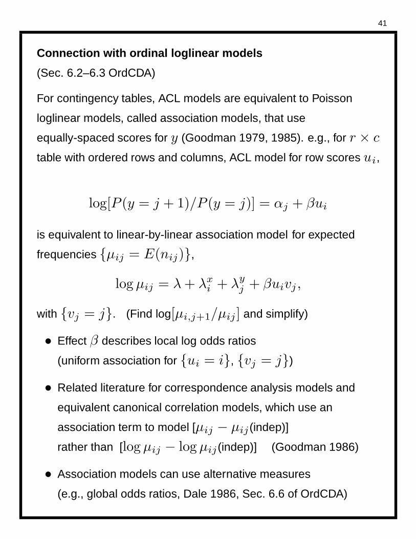
Connection with ordinal loglinear models
(Sec. 6.2–6.3 OrdCDA)
For contingency tables, ACL models are equivalent to Poisson
loglinear models, called association models, that use
equally-spaced scores for y (Goodman 1979, 1985). e.g., for r × c
table with ordered rows and columns, ACL model for row scores ui,
log[P (y = j + 1)/P (y = j)] = αj + βui
is equivalent to linear-by-linear association model for expected
frequencies µij = E(nij),
log µij = λ + λxi + λy
j + βuivj ,
with vj = j. (Find log[µi,j+1/µij ] and simplify)
• Effect β describes local log odds ratios
(uniform association for ui = i, vj = j)
• Related literature for correspondence analysis models and
equivalent canonical correlation models, which use an
association term to model [µij − µij (indep)]
rather than [log µij − log µij (indep)] (Goodman 1986)
• Association models can use alternative measures
(e.g., global odds ratios, Dale 1986, Sec. 6.6 of OrdCDA)

42
b. Models using continuation-ratio logits(Sec. 4.2 of OrdCDA)
log[P (yi = j)/P (yi ≥ j + 1)], j = 1, ..., c − 1, or
log[P (yi = j + 1)/P (yi ≤ j)], j = 1, ..., c − 1
Let ωj = P (y = j | y ≥ j) =πj
πj+···+πc
Then
log
(
πj
πj+1 + · · · + πc
)
= log[ωj/(1 − ωj)],
• Of interest when a sequential mechanism determines the
response outcome (Tutz 1991) or for grouped survival data
(Prentice and Gloeckler 1978)
• Simple model with proportional odds structure is
logit[ωj(x)] = αj + β′
x, j = 1, . . . , c − 1,
• More general model logit[ωj(x)] = αj + β′
jx
has fit equivalent to fit of c − 1 separate binary logit models,
because multinomial factors into binomials,
p(yi1, . . . , yic) = p(yi1)p(yi2 | yi1) · · · p(yic | yi1, . . . , yi,c−1) =
bin[1, yi1; ω1(xi)] · · · bin[1 − yi1 − · · · − yi,c−2, yi,c−1; ωc−1(xi)].

43
Example: Tonsil Size and Streptococcus
Tonsil Size
Carrier Not enlarged Enlarged Greatly Enlarged
Yes 19 (26%) 29 (40%) 24 (33%)
No 497 (37%) 560 (42%) 269 (20%)
Let x = whether carrier of Streptococcus pyogenes (1 = yes, 0 = no)
Continuation-ratio logit model fits well (deviance 0.01, df = 1):
log
[
π1
π2 + π3
]
= α1 + βx, log
[
π2
π3
]
= α2 + βx
has β = −0.528 (SE = 0.196). Model estimates an assumed
common value exp(−0.528) = 0.59 for cumulative odds ratio
from first part of model and for local odds ratio from second part.
e.g., given that tonsils were enlarged, for carriers, estimated odds
of response enlarged rather than greatly enlarged were 0.59 times
estimated odds for non-carriers.
By contrast, cumulative logit model estimates
exp(−0.6025) = 0.55 for each cumulative odds ratio, and ACL
model estimates exp(−0.429) = 0.65 for each local odds ratio.
(Both these models also fit well: Deviances 0.30, 0.24, df = 1.)

44
-------------------------------------------------------------------------------
data tonsils; * look at data as indep. binomials;
input stratum carrier success failure;
n = success + failure;
datalines;
1 1 19 53
1 0 497 829
2 1 29 24
2 0 560 269
;
proc genmod data=tonsils; class stratum;
model success/n = stratum carrier / dist=binomial link=logit lrci type3;
run;
-----------------------------------------------------------------------
Analysis Of Parameter Estimates
Likelihood Ratio
Standard 95% Confidence Chi-
Parameter DF Estimate Error Limits Square
Intercept 1 0.7322 0.0729 0.5905 0.8762 100.99
stratum 1 1 -1.2432 0.0907 -1.4220 -1.0662 187.69
stratum 2 0 0.0000 0.0000 0.0000 0.0000 .
carrier 1 -0.5285 0.1979 -0.9218 -0.1444 7.13
LR Statistics For Type 3 Analysis
Chi-
Source DF Square Pr > ChiSq
carrier 1 7.32 0.0068

45
Adjacent Categories Logit and Continuation Ratio Logit
Models with Nonproportional Odds
• As in cumulative logit case, model of proportional odds form fits
poorly when there are substantive dispersion effects
• Each model has a more general non-proportional odds form,
the ACL version being
log[P (yi = j)/P (yi = j + 1)] = αj + β′jxi
• Unlike cumulative logit model, these models do not have
structural problem of out-of-order cumulative probabilities
• Models lose ordinal advantage of parsimony, but effects still
have ordinal nature, unlike BCL models
• Can fit general ACL model with software for BCL model,
converting its β∗j estimates to βj = β∗
j − β∗j+1, since
log
(
πj
πj+1
)
= log
(
πj
πc
)
− log
(
πj+1
πc
)
.

46
c. Stereotype model: Multiplicative paired-categorylogits(Sec. 4.3 of OrdCDA)
ACL model with separate effects for each pair of adjacent
categories is equivalent to standard BCL model
log
[
πj
πc
]
= αj + β′
jx, j = 1, . . . , c − 1.
• Disadvantage: lack of parsimony (treats response as nominal)
• c − 1 parameters for each predictor instead of a single
parameter
• No. parameters large when either c or no. of predictors large
Anderson (1984) proposed alternative model nested between ACL
model with proportional odds structure and the general ACL or BCL
model with separate effects βj for each logit.

47
Stereotype model :
log
[
πj
πc
]
= αj + φjβ′
x, j = 1, . . . , c − 1.
• For predictor xk , φjβk represents log odds ratio for
categories j and c for a unit increase in xk . By contrast,
general BCL model has log odds ratio βjk for this effect, which
requires many more parameters
• φj are parameters, treated as “scores” for categories of y.
• Like proportional odds models, stereotype model has
advantage of single parameter βk for effect of predictor xk
(for given scores φj).
• Stereotype model achieves parsimony by using same scores
for each predictor, which may or may not be realistic.
• Identifiability requires location and scale constraints on φj,
such as (φ1 = 1, φc = 0) or (φ1 = 0, φc = 1).
• Corresponding model for category probabilities is
P (yi = j) =exp(αj + φjβ
′
xi)
1 +∑c−1
k=1 exp(αk + φkβ′
xi)
• Model is multiplicative in parameters, which makes model
fitting awkward
(gnm add-on function to R fits this and other nonlinear models).

48
d. Cumulative Probit Models (Sec. 5.2 of OrdCDA)
Denote cdf of standard normal by Φ.
Cumulative probit model is
Φ−1[P (y ≤ j)] = αj + β′x, j = 1, . . . , c − 1
e.g., P (y ≤ j) = 1/2 when αj + β′x = 0
since Φ(0) = 1/2 = P (standard normal r.v. < 0)
As in proportional odds models (logit link), effect β is same for
each cumulative probability.
(Here, not appropriate to call this a “proportional odds” model,
because interpretations do not apply to odds or odds ratios.)

49
Properties
• Motivated by underlying normal regression model for latent
variable y∗ with constant σ (WLOG, can set σ = 1).
• Then, coefficient βk of xk has interpretation that a unit
increase in xk corresponds to change in E(y∗) of βk (change
of βk standard deviation, when σ 6= 1), keeping fixed other
predictor values.
• Logistic and normal cdfs having same mean and standard
deviation look similar, so cumulative probit models and
cumulative logit models fit well in similar situations.
• Standard logistic distribution G(y) = ey/(1 + ey) has mean
0 and standard deviation π/√
3 = 1.8. ML estimates from
cumulative logit models tend to be about 1.6 to 1.8 times ML
estimates from cumulative probit models.
• Quality of fit and statistical significance essentially same for
cumulative probit and cumulative logit models. Both imply
stochastic orderings at different x levels and are designed to
detect location rather than dispersion effects.

50
Example: Religious fundamentalism by highest educational
degree (GSS data from 1972 to 2006, huge n)
Religious Beliefs
Highest Degree Fundamentalist Moderate Liberal
Less than high school 4913 (43%) 4684 (41%) 1905 (17%)
High school 8189 (32%) 11196 (44%) 6045 (24%)
Junior college 728 (29%) 1072 (43%) 679 (27%)
Bachelor 1304 (20%) 2800 (43%) 2464 (38%)
Graduate 495 (16%) 1193 (39%) 1369 (45%)
For cumulative link model
link[P (y ≤ j)] = αj + βxi
using scores xi = i for highest degree,
β = −0.206 (SE = 0.0045) for probit link
β = −0.345 (SE = 0.0075) for logit link

51
-----------------------------------------------------------------------
data religion;
input degree religion count;
datalines;
0 1 4913
0 2 4684
0 3 1905
1 1 8189
1 2 11196
1 3 6045
...
4 3 1369
;
proc logistic; weight count;
model religion = degree / link=probit aggregate scale=none;
----------------------------------------------------------------------
Score Test for the Equal Slopes Assumption
Chi-Square DF Pr > ChiSq
0.2452 1 0.6205
Deviance and Pearson Goodness-of-Fit Statistics
Criterion Value DF Value/DF Pr > ChiSq
Deviance 48.7072 7 6.9582 <.0001
Pearson 48.9704 7 6.9958 <.0001
Model Fit Statistics
Intercept
Intercept and
Criterion Only Covariates
AIC 105532.77 103395.09
SC 105534.19 103397.21
-2 Log L 105528.77 103389.09
Standard Wald
Parameter DF Estimate Error Chi-Square Pr > ChiSq
Intercept 1 1 -0.2240 0.00799 785.6659 <.0001
Intercept 2 1 0.9400 0.00868 11736.5822 <.0001
degree 1 -0.2059 0.00447 2120.0908 <.0001
-----------------------------------------------------------------------

52
• From probit β = −0.206, for category increase in highest
degree, mean of underlying response on religious beliefs
estimated to decrease by 0.21 standard deviations.
• From logit β = −0.345, estimated odds of response in
fundamentalist rather than liberal direction multiply by
exp(−0.345) = 0.71 for each category increase in degree.
e.g., estimated odds of fundamentalist rather than moderate or
liberal for those with less high school education are
1/ exp[4(−0.345)] = 4.0 times estimated odds for those
with graduate degree.
For each category increase in highest degree, mean of
underlying response on religious beliefs estimated to decrease
by 0.345/(π/√
3) = 0.19 standard deviations.
Goodness of fit?
Cumulative probit: Deviance = 48.7 (df = 7)
Cumulative logit: Deviance = 45.4 (df = 7)
Either link treating education as factor passes goodness-of-fit test,
but fit not practically different than with simpler linear trend model.
e.g., Probit deviance = 5.2, logit deviance = 2.4 (df = 4)
Probit β1 = 0.83, β2 = 0.56, β3 = 0.46, β4 = 0.17, β5 = 0

53
e. Cumulative Log-Log Links (Sec. 5.3 of OrdCDA)
Logit and probit links have symmetric S shape, in sense that
P (y ≤ j) approaches 1.0 at same rate as it approaches 0.0.
Model with complementary log-log link
log− log[1 − P (y ≤ j)] = αj + β′x
approaches 1.0 at faster rate than approaches 0.0. It and
corresponding log-log link,
log− log[P (y ≤ j)],
based on underlying skewed distributions (extreme value) with cdf
of form G(y) = exp− exp[−(y − a)/b].
• Model with complementary log-log link has interpretation that
P (y > j | x with xk = x+1) = P (y > j | x with xk = x)exp(βk)
• Most software provides complementary log-log link, but can fit
model with log-log link by reversing order of categories and
using complementary log-log link.

54
Example: Life table for gender and race (percent)
Males Females
Life Length White Black White Black
0-20 1.3 2.6 0.9 1.8
20-40 2.8 4.9 1.3 2.4
40-50 3.2 5.6 1.9 3.7
50-65 12.2 20.1 8.0 12.9
Over 65 80.5 66.8 87.9 79.2
Source: 2008 Statistical Abstract of the United States
For gender g (1 = female; 0 = male), race r (1 = black; 0 = white),
and life length y, consider model
log− log[1 − P (y ≤ j)] = αj + β1g + β2r
Good fit with this model or a cumulative logit model or a cumulative
probit model

55
data lifetab;
input sex $ race $ age count;
datalines;
m w 20 13
f w 20 9
m b 20 26
f b 20 18
m w 40 28
f w 40 13
m b 40 49
f b 40 24
m w 50 32
f w 50 19
m b 50 56
f b 50 37
m w 65 122
f w 65 80
m b 65 201
f b 65 129
m w 100 805
f w 100 879
m b 100 668
f b 100 792
;
proc logistic; weight count; class sex race / param=ref;
model age = sex race / link=cloglog aggregate scale=none;
run;
proc genmod; weight count; class sex race;
model age = sex race / dist=multinomial link=CCLL lrci type3 obstats;
run;
-----------------------------------------------------------------------------
The GENMOD Procedure
Analysis Of Parameter Estimates
Likelihood Ratio
Standard 95% Confidence Chi-
Parameter DF Estimate Error Limits Square
Intercept1 1 -4.2127 0.1338 -4.4840 -3.9587 991.04
Intercept2 1 -3.1922 0.0911 -3.3741 -3.0168 1226.85
Intercept3 1 -2.5821 0.0764 -2.7340 -2.4347 1143.60
Intercept4 1 -1.5216 0.0623 -1.6458 -1.4015 596.43
sex f 1 -0.5383 0.0703 -0.6769 -0.4011 58.57
sex m 0 0.0000 0.0000 0.0000 0.0000 .
race b 1 0.6107 0.0709 0.4725 0.7506 74.20
race w 0 0.0000 0.0000 0.0000 0.0000 .

56
β1 = −0.538, β2 = 0.611
Gender effect:
P (y > j | g = 0, r) = [P (y > j | g = 1, r)]exp(0.538)
Given race, proportion of men living longer than a fixed time equals
proportion for women raised to exp(0.538) = 1.71 power.
Given gender, proportion of blacks living longer than a fixed time
equals proportion for whites raised to exp(0.611) = 1.84 power.
Cumulative logit model has gender effect = −0.604, race effect =
0.685.
If Ω denotes odds of living longer than some fixed time for white
women, then estimated odds of living longer than that time are
exp(−0.604)Ω = 0.55Ω for white men
exp(−0.685)Ω = 0.50Ω for black women
exp(−0.604 − 0.685)Ω = 0.28Ω for black men

57
f. Modeling Non-Standard Count Data
• Count responses often have zero inflation
e.g., number of medical appointments a subject had in past
year; some subjects have 0 observation as result of chance,
others because of doctor-avoidance phobia or (in U.S.) cost
and/or lack of medical insurance.
• Models for clustered zero-inflated count data include
(a) hurdle model that uses logistic regression to model whether
an observation is zero or positive and a separate loglinear
model with a truncated distribution for the positive counts
(b) a zero-inflated Poisson model that for each observation
uses a mixture of a Poisson loglinear model and a degenerate
distribution at 0
(c) a zero-inflated negative binomial model that allows
overdispersion relative to the zero-inflated Poisson model.
• Model (a) requires separate parameters for the effects of
explanatory variables in the logistic model and in the loglinear
model.
• Models (b) and (c) require separate parameters for the effects
of explanatory variables on the mixture probability and in the
loglinear model.

58
• The models can encounter fitting difficulties if there is
zero-deflation at any settings of explanatory variables.
• When Yt has relatively few distinct count outcomes, simple
alternative approach applies a cumulative logit random effects
model to the count data (Min and Agresti 2005).
• The first category is the zero outcome and each other count
outcome is a separate category
• When large number of count values recorded, collapse into
ordered categories (at least 4 categories to avoid power loss)
• This approach has advantage of single set of parameters for
describing effects. Those parameters describe effects overall,
rather than conditional on a response being positive.

59
Modeling Repeated Measures of Zero-Inflated Data
ex. Pharmaceutical study comparing two treatments for a disease
with 118 patients, half randomly allocated to each treatment.
Response = number of episodes of a certain side effect, with this
count observed at six times.
Side Effect Frequencies for Treatment A and Treatment B
Frequencies
Treatment 0 1 2 3 4 5 6
A 312 30 11 0 1 0 0
B 278 39 20 6 7 2 2
Total 590 69 31 6 8 2 2
Complete data and SAS code for various analyses at
www.stat.ufl.edu/∼aa/ordinal/ord.html
Other explanatory variable: time elasped since previous
observation.
Min and Agresti showed strong evidence of zero inflation for
standard models for counts, such as Poisson model with a random
intercept.

60
For ordinal approach, group Yt into (0, 1, 2, 3, 4, > 4)
Random effects model: For subject i,
logit[P (Yit ≤ j)] = ui+αj+β1tr+β2 log(time), j = 0, . . . , 4,
where tr is indicator for whether the subject uses treatment A.
From analysis discussed in text (p. 292) with independent random
effects ui ∼ N(0, σ2) integrated out to get likelihood,
β1 = 0.977 has SE = 0.431
At each observation time and for a fixed time elapsed since
previous observation, estimated odds that number of side effects
falls below any fixed level with treatment A are
exp(0.977) = 2.66 times estimated odds for treatment B.
Estimate σu = 1.73 (with SE = 0.25) of variability among uisuggests considerable within-subject positive correlation among
the repeated responses.

61
Bayesian Ordinal Data Analysis(Chapter 11 of OrdCDA)
Recall the posterior density function is proportional to the product
of the prior density function with the likelihood function.
Some highlights:
• For multinomial data, Dirichlet distribution serves as conjugate
prior over (π1, . . . , πc) probability simplex. Useful for
smoothing contingency tables (Lindley 1964, Good 1965).
• For 2 × c ordinal table with two independent Dirichlet priors,
Altham (1969) derived expression for posterior probability that
one distribution is stochastically larger than the other. (p. 336
OrdCDA)
• Logistic-normal prior (multivariate normal for vector of logits)
adapts better to ordinality and is more flexible, through, e.g.,
Corr[logit(πa), logit(πb)] = ρ|a−b|
(Leonard 1973, smoothing a histogram)

62
Bayesian Approaches with Ordinal Models
• For modeling, in which parameters β are real-valued, using a
multivariate normal prior provides broad scope. Prior is
non-informative when prior σ values large (e.g., 1000).
• Posterior distributions approximated using MCMC methods
(e.g., with software such as WinBUGS), most simply using
methods for normal responses based on latent variable
connections (Albert and Chib 1993, P. Hoff 2009 First Course
in Bayesian Statistical Methods, Ch. 12)
• SAS ver. 9.2 has BAYES option in PROC GENMOD, for
univariate Y (e.g., binomial, Poisson, normal) but not
multinomial. (Sec. 11.3.5, 11.3.6 of OrdCDA)
Can fit (1) continuation-ratio logit model using connection
between multinomial and a product of binomials , (2)
adjacent-categories logit model using connection with Poisson
loglinear model.
• Priors for cumulative logit models should recognize constraint
α1 < α2 < · · · < αc−1. Sec. 11.3.4 of OrdCDA shows ex.,
also summarizing by posterior P (β > 0), P (β < 0). Table
A.8 (p. 353) shows PROC MCMC for Bayesian analysis.

63
Example: Tonsil Size and Streptococcus
Tonsil Size
Carrier Not enlarged Enlarged Greatly Enlarged
Yes 19 (26%) 29 (40%) 24 (33%)
No 497 (37%) 560 (42%) 269 (20%)
Continuation-ratio logit model
log
[
π1
π2 + π3
]
= α1 + βx, log
[
π2
π3
]
= α2 + βx
where x = whether carrier of Streptococcus pyogenes
β is a cumulative log odds ratio for the 2×2 table comparing
column 1 to columns 2 and 3 combined (first logit) and a local log
odds ratio for the 2×2 table consisting of columns 2 and 3 (second
logit).
Use normal priors for model parameters with means of 0.
For x, let 0.5 = yes, −0.5 = no (instead of 1 = yes and 0 = no), so
the logit has the same prior variability for each logit.

64
-------------------------------------------------------------------------------
data tonsils; * look at data as indep. binomials;
input stratum carrier success failure;
n = success + failure; carrier2 = carrier - 0.5; * symmetrize prior
datalines;
1 1 19 53
1 0 497 829
2 1 29 24
2 0 560 269
;
proc genmod data=tonsils; class stratum; * frequentist analysis;
model success/n = stratum carrier / dist=binomial link=logit lrci type3;
proc genmod data=tonsils; class stratum; * Bayesian analysis;
model success/n = stratum carrier2 / dist=binomial link=logit;
bayes coeffprior=normal initialmle diagnostics=mcerror nmc=2000000;
run; * noninformative, takes prior std dev = 1000 for all parameters;
proc genmod data=tonsils; class stratum; * Bayesian analysis;
model success/n = stratum carrier2 / dist=binomial link=logit;
bayes coeffprior=normal (var=1.0) initialmle diagnostics=mcerror nmc=2000000;
run; *informative, takes prior std dev = 1 for all parameters;
-------------------------------------------------------------------------------
Posterior Estimates of β. Results in ML row are ML estimate, SE, and
95% profile likelihood confidence interval.
Prior Distribution Mean Std Dev 95% Credible Interval
Normal (σ = 1000) −0.533 0.199 (−0.926, −0.146)
Normal (σ = 1.0) −0.518 0.194 (−0.902, −0.141)
ML −0.5285 0.198 (−0.922, −0.144)
Note: HPD credible interval ok for β model parameters, but not sensible for
odds ratios eβ .

65
Summary
• Logistic regression for binary responses extends in various
ways to handle ordinal responses: Use logits for cumulative
probabilities, adjacent-response categories, continuation ratios.
Stereotype model can treat baseline-category logits ordinally.
• Other ordinal multinomial models include cumulative link
models (probit, complementary-log-log), and it can be useful to
handle count data with a multinomial model.
• Which model to use? Apart from certain types of data in which
grouped response models are invalid (e.g., cumulative logits
with case-control data), we may consider (1) how we want to
summarize effects (e.g., cumulative prob’s with cumulative
logit, individual category prob’s with ACL) and (2) do we want a
connection with an underlying latent variable model (natural
with cumulative logit and other cumulative link models)?
• Models extend to multivariate responses using marginal
models and mixed models with random effects (Chap. 8-10).
• Other methods require assigning fixed or midrank scores to
response categories, such as extensions of nonparametric
methods to allow for the ties that occur with ordinal data.

66
3 Software for Ordinal Modeling
See OrdCDA appendix for details, and also some details for SPSS
(not covered here).
SAS
• PROC FREQ provides large-sample and small-sample tests of
independence in two-way tables, measures of association and
their estimated SEs, and generalized CMH tests of conditional
independence.
• PROC GENMOD fits multinomial cumulative link models and
Poisson loglinear models , and it can perform GEE analyses for
marginal models as well as Bayesian model fitting for binomial
and Poisson data.
• PROC LOGISTIC fits cumulative link models.
• PROC NLMIXED fits models with random effects and
generalized nonlinear models (e.g., stereotype model).
• PROC CATMOD can fit baseline-category logit models by ML,
and hence adjacent-category logit models.

67
R (and S-Plus)
• A detailed discussion of the use of R for models for categorical
data is available on-line in the free manual prepared by Laura
Thompson to accompany Agresti (2002). A link to this manual
is at www.stat.ufl.edu/∼aa/cda/software.html.
• Specialized R functions available from various R libraries. Prof.
Thomas Yee at Univ. of Auckland provides VGAM for vector
generalized linear and additive models
(www.stat.auckland.ac.nz/∼yee/VGAM).
• In VGAM, the vglm function fits wide variety of models.
Possible models include the cumulative logit model (family
function cumulative) with proportional odds or partial
proportional odds or nonproportional odds, cumulative link
models (family function cumulative) with or without common
effects for each cutpoint, adjacent-categories logit models
(family function acat), and continuation-ratio logit models
(family functions cratio and sratio).

68
• Many other R functions can fit cumulative logit and other
cumulative link models. Thompson’s manual (p. 121) describes
the polr function from the MASS library. The syntax is simple,
such aslibrary(MASS)
fit.cum <- polr(y ˜ x, data=tab3.1, method=‘‘probit’’)
summary(fit.cum)
• The package gee contains a function gee for ordinal GEE
analyses. The package geepack contains a function ordgee for
ordinal GEE analyses.
• The package glmmAK contains a function cumlogitRE for using
MCMC to fit cumulative logit models with random effects.
• Can fit nonlinear models such as stereotype model using gnm
add-on function to R by Firth and Turner:
www2.warwick.ac.uk/fac/sci/statistics/staff/research/turner/gnm/
• R function mph.fit prepared by Joe Lang at Univ. of Iowa can fit
many models for contingency tables that are difficult to fit with
ML, such as mean response models, global odds ratio models,
marginal models.

69
Stata
• The ologit program (www.stata.com/help.cgi?ologit) fits
cumulative logit models.
• The oprobit program (www.stata.com/help.cgi?oprobit) fits
cumulative probit models.
• Continuation-ratio logit models can be fitted with the ocratio
module (www.stata.com/search.cgi?query=ocratio) and with
the seqlogit module
• The stereotype model can be fitted with the slogit program
(www.stata.com/help.cgi?slogit).
• The GLLAMM module (www.gllamm.org) can fit a very wide
variety of models, including cumulative logit models with
random effects. See www.stata.com/search.cgi?query=gllamm.

70
4 Other Work on Modelling Ordinal
Responses
No attempt to be complete; see text notes at end of each chapter of
OrdCDA for more references.
Modelling Association
Association models – Anderson and Vermunt (2000), Becker (1989),
Becker and Clogg (1989), Gilula, Krieger and Ritov (1988), Goodman
(1985), Haberman (1981), Kateri, Ahmad, and Papaioannou (1998),
Rom and Sarkar (1992)
Square contingency tables and extensions – Agresti (1993), Agresti and
Lang (1993), Becker (1990), Dale (1986), Ekholm et al. (2003), Kateri
and Agresti (1997), Kateri and Papaioannou (1997), Sarkar (1989),
Williamson, Kim, and Lipsitz (1995)
Correspondence analysis, correlation models – Beh (1997), Gilula
(1986), Gilula and Ritov (1990), Goodman (1986), Goodman (1996),
Ritov and Gilula (1993)
Modelling Agreement
Latent trait models – e.g., Uebersax and Grove (1993), Yang and Becker
(1997)
Loglinear and association models – Agresti (1988), Becker (1989, 1990),

71
Becker and Agresti (1992), Schuster and von Eye (2001), Valet,
Guinot, and Mary (2007)
Random effects – Williamson and Manatunga (1997)
ROC and related methods – Toledano and Gatsonis (1996), Ishwaran
and Gatsonis (2000)
Measures of agreement – Banerjee et al. (1999), Roberts and McNamee
(2005)
Multivariate Models
Marginal models – Heagerty and Zeger (1996), Lipsitz, Kim, and Zhao
(1994), Molenberghs and Lesaffre (1994, 1999), Lang, McDonald, and
Smith (1999), Lumley (1996), Stram, Wei, and Ware (1988), Ten Have,
Landis, and Hartzel (1998)
Random effects models – Ezzet and Whitehead (1991), Hartzel, Agresti,
and Caffo (2001), Hedeker and Gibbons (1994), Tutz and Hennevogl
(1996), Liu and Hedeker (2006), Ten Have et al. (2000), Xie, Simpson,
and Carroll (2000)
Multilevel models – Fielding and Lang (2005), Gibbons and Hedeker
(1997), Grilli and Rampichini (2003, 2007), Steele and Goldstein
(2006), Zaslavsky and Bradlow (1999)
Nonparametric sorts of inference
Inference using rank statistics – Akritas and Brunner (1997), Bathke and

72
Brunner (2003), Brunner and Puri (2001, 2002), Rayner and Best
(2001)
Nonparametric random effects – Hartzel, Agresti, and Caffo (2001)
Bayesian Inference
Modelling an ordinal response – Lang (1999), Johnson and Albert (1999),
Hoff (2009, Ch. 12)
Multivariate ordinal responses, hierarchical models – Albert and Chib
(1993, 2001), Bradlow and Zaslavsky (1999), Cowles et al. (1996),
Kaciroti et al. (2006), Qu and Tan (1998)
Association models – Iliopoulos, Kateri, and Ntzoufras (2007), Kateri,
Nicolaou, and Ntzoufras (2005)
Case-control analyses with an ordinal response – Mukherjee et al. (2007,
2008), Mukherjee and Liu (2008)
Small-Sample Inference
Exact tests of independence and conditional independence for ordinal
variables – Agresti, Mehta and Patel (1990 and linear-by-linear option
in StatXact), Kim and Agresti (1997), Agresti and Coull (1998)
Improved tests from a decision-theoretic perspective – Cohen and
Sackrowitz (1991), Berger and Sackrowitz (1997)
Higher-order approximations such as the saddlepoint essentially exact for
single-parameter inference – Pierce and Peters (1992), Agresti, Lang,

73
and Mehta (1993)
Goodness of Fit
Chi-squared statistics inappropriate with continuous predictors or highly
sparse data
Generalization of Hosmer-Lemeshow statistic – Lipsitz, Fitzmaurice,
Molenberghs (1996)
For cumulative logit models, can test proportional odds assumption –
Brant (1990), Peterson and Harrell (1990)
Goodness-of-link testing – Genter and Farewell (1985)
Missing Data
Accounting for drop out – Molenberghs, Kenward, and Lesaffre (1997),
Ten Have et al. (2000)
Score test of independence in two-way tables with ordered categories
and extensions for stratified data – Lipsitz and Fitzmaurice (1996)
Comparison of likelihood-based and GEE methods for repeated ordinal
responses – Mark and Gail (1994), Kenward, Lesaffre, and
Molenberghs (1994)
Order-Restricted Inference
Estimate cell proportions (and conduct tests) assuming solely that a type
of ordinal log odds ratio is uniformly nonnegative

74
Local odds ratios – Patefield (1982), Dykstra et al. (1995), Agresti and
Coull (1998)
Cumulative odds ratios – Grove (1980), Robertson and Wright (1981),
Cohen and Sackrowitz (1996), Evans et al. (1997)
Order restrictions on parameters in association models – Agresti, Chuang
and Kezouh (1987), Galindo-Garre and Vermunt (2004), Iliopoulos,
Kateri, and Ntzoufras (2007), Ritov and Gilula (1991, 1993)
Marginal modeling – Bartolucci et al. (2001), Bartolucci and Forcina
(2002), Colombi and Forcina (2001)
Detailed references are in Bibliography of OrdCDA.
Other areas not discussed here include other model diagnostics,
smoothing ordinal data (e.g., generalized additive models), paired
preference modeling, survival modeling. Can find some info by looking up
the topic in Subject Index of OrdCDA.

75
Partial Bibliography: Analysis of Ordinal Categorical Data
Some Books
Agresti, A. 2010. Analysis of Ordinal Categorical Data, Wiley, 2nd ed.
Clogg and Shihadeh (1994). Statistical Models for Ordinal Variables, Sage.
Fahrmeir, L., and G. Tutz. 2001. Multivariate Statist. Modelling based on Generalized Linear Models, 2nd ed. Springer-Verlag.
Johnson, V. E., and J. H. Albert 1999. Ordinal Data Modeling. Springer.
McCullagh, P., and J. A. Nelder. 1983, 2nd edn. 1989. Generalized Linear Models. London: Chapman and Hall.
Some Survey Articles
Agresti, A. 1999. Modelling ordered categorical data: Recent advances and future challenges. Statist. Medic. 18: 2191–2207.
Agresti, A., and R. Natarajan. 2001. Modeling clustered ordered categorical data: A survey. Intern. Statist. Rev., 69: 345-371.
Anderson, J. A. 1984. Regression and ordered categorical variables. J. Roy. Statist. Soc. B 46: 1–30.
Chuang-Stein, C. and A. Agresti. 1997. A review of tests for detecting a monotone dose-response relationship with ordinal
responses data. Statist. Medic. 16: 2599–2618.
Goodman, L. A. 1979. Simple models for the analysis of association in cross-classifications having ordered categories. J. Amer.
Statist. Assoc. 74: 537–552.
Goodman, L. A. 1985. The analysis of cross-classified data having ordered and/or unordered categories: Association models,
correlation models, and asymmetry models for contingency tables with or without missing entries. Ann. Statist. 13: 10–69.
Landis, J. R., E. R. Heyman, and G. G. Koch. 1978. Average partial association in three-way contingency tables: A review and
discussion of alternative tests. Internat. Statist. Rev. 46: 237–254.
Liu, I., and A. Agresti. 2005. The analysis of ordered categorical data: An overview and a survey of recent developments (with
discussion). Test 14: 1–73.
McCullagh, P. 1980. Regression models for ordinal data. 42: J. Royal. Stat. Society, B, 109–142.