Embed Size (px)
Citation preview

Master of Science Thesis
Modeling of Subcooled Nucleate Boiling with OpenFOAM
Edouard Michta
Supervisors:Henryk AnglartKristian Angele
Division of Nuclear Reactor TechnologyRoyal Institute of Technology
Stockholm, Sweden, February 2011
TRITA-FYS 2011:11 ISSN 0280-316X ISRN KTH/FYS/–11:10–SE

ii

ABSTRACT
Within the course of this master thesis project, subcooled nucleate boiling in a vertical pipe has been modeledusing CFD. The modeling has been carried out within the OpenFOAM framework and a two-phase Eulerianapproach has been chosen. The code can be used to predict the distribution of the local flow parameters, i.e.the void fraction, the bubble diameter, the velocity of both liquid and gas, the turbulent intensity as well asthe liquid temperature. Special attention has been devoted to the phenomena which govern the void fractiondistribution in the radial direction. Two different solvers have been implemented and the simulations havebeen performed in two dimensions.
Firstly, isothermal turbulent bubbly flow is mechanistically modeled in a solver named myTwoPhaseEulerFoa-mAdiabatic. The conservation equations of mass and momentum are solved for the two phases, taking specialcare in the modeling of the interfacial forces. The turbulence phenomena are described by a classical k-εmodel in combination with standard wall functions for the near-wall treatment. Furthermore, an interfacialarea concentration equation is solved and two different models for its sink- and source terms (correspondingto bubble coalesence and bubble breakup) have been investigated.
Secondly, a solver named myTwoPhaseEulerFoamBoiling has been developed based on the first solver in orderto model a heated wall leading to subcooled nucleate boiling and subsequent condensation in the subcooledliquid. Additional terms accounting for the phase change have been included in the mass and momentumconservation equations as well as in the interfacial area equation. Assuming the gas phase being at saturationconditions, only one energy equation for the liquid phase needs to be solved.
The adiabatic solver has been validated against the DEDALE experiment and the simulation results showedsatisfactory agreement with the measured data. The predictions obtained from myTwoPhaseEulerFoam-Boiling have been compared to the DEBORA experimental data base. They are qualitatively similar butrather high quantitative discrepancies exist. Grid dependence tests revealed that the latter solver dependson the near-wall grid resolution, a yet unresolved issue related to the application of the wall heat flux asthe boundary condition. However, the results were shown to be insensitive to small variations in the appliedinlet conditions.
iii

iv

ACKNOWLEDGEMENTS
Summarising a 18-month experience in one single page is impossible. There are too many people I wouldlike to thank for having helped me in my work or shared very nice moments with. Long story short...
First of all, I would like to thank Henryk Anglart for having continuously helped and guided me throughoutthis thesis. I am also very grateful to all the colleagues at the Nuclear Reactor Technology department for thenice atmosphere I discovered there, as well as the interesting discussions we could have during our bi-weeklymeeting. Vielen Dank especially to Roman for having standed me coming to his office every hour to ask himsilly questions rearding OpenFOAM or Linux, but also for these great pingis nights I will miss so much andfor the camels...
Furthermore, I am indebted to Vattenfall for the financial support but also for having welcomed me sowarmly at their facility in Alvkarleby. Particularly, I would like to express my gratitude to Kristian Angelefor his constant availability and for having given me valuable input or feedback in my work. The friendlyand respectful relation we have had is probably one of the main reasons of the successfull outcome of thisproject.
In addition, I had a great year living almost 24/7 with Herve, Marc, Mathias and Pauline (who by the waysaved us from eating a Paneng every day...) and with whom I did so many memorable trips and organisedan unforgettable corridor party! Also I must mention all the nukes for the year and a half we have spenttogether at Albanova, so Fredrik, Luca, Marti, Paul and all the others, I hope to see you soon again! Aswell I want to thank all my friends at Supaero, and I would like to recall this unique experience we sharedwith a few of them on a boat to Tallinn... A big Thank ya! to the 9BD crew, notably to Bastien, Bastien,JB, Alexane and Marc, for all the amazing nights quite often ending at Max... Besides, I am also very gladhaving been a team member of Los Cachondos, so thanks guys for the games, the beers and my first title inSweden! Still about football, I will always remember this match with PE, Val and Alexandre played around4 am, I am pretty sure you will never forget it neither... I am also very glad I got to know Eline better inthe last months of my stay in Sweden, she will certainly remain a friend for long. There are still too manypeople I have not cited: my awesome roomie Johan of course but also Marta-Linn, Ludvig, Julia, Josefineand all the others I cannot mention for brevity reasons.
Finally, I want above all to thank my family, who has always supported my choices and has given me thisunique opportunity to discover such a beautiful country that is Sweden and that I fell in love with.
v

vi

CONTENTS
1 Introduction 1
1.1 Background . . . . . . . . . . . . . . . . . . . . . . . . . . . . . . . . . . . . . . . . . . . . . . 1
1.2 Subcooled nucleate boiling . . . . . . . . . . . . . . . . . . . . . . . . . . . . . . . . . . . . . . 1
1.3 Computational fluid dynamics (CFD) . . . . . . . . . . . . . . . . . . . . . . . . . . . . . . . 2
1.4 Objectives of the work . . . . . . . . . . . . . . . . . . . . . . . . . . . . . . . . . . . . . . . . 3
2 Mathematical model description 5
2.1 Governing flow equations . . . . . . . . . . . . . . . . . . . . . . . . . . . . . . . . . . . . . . 5
2.2 Interfacial forces . . . . . . . . . . . . . . . . . . . . . . . . . . . . . . . . . . . . . . . . . . . 6
2.2.1 Drag force . . . . . . . . . . . . . . . . . . . . . . . . . . . . . . . . . . . . . . . . . . . 6
2.2.2 Lift force . . . . . . . . . . . . . . . . . . . . . . . . . . . . . . . . . . . . . . . . . . . 7
2.2.3 Wall lubrication force . . . . . . . . . . . . . . . . . . . . . . . . . . . . . . . . . . . . 8
2.2.4 Turbulent dispersion force . . . . . . . . . . . . . . . . . . . . . . . . . . . . . . . . . . 8
2.2.5 Virtual mass force . . . . . . . . . . . . . . . . . . . . . . . . . . . . . . . . . . . . . . 9
2.3 Boiling model . . . . . . . . . . . . . . . . . . . . . . . . . . . . . . . . . . . . . . . . . . . . . 9
2.3.1 Wall heat flux partitioning . . . . . . . . . . . . . . . . . . . . . . . . . . . . . . . . . 9
2.3.2 Nucleation site density . . . . . . . . . . . . . . . . . . . . . . . . . . . . . . . . . . . . 10
2.3.3 Detachment frequency . . . . . . . . . . . . . . . . . . . . . . . . . . . . . . . . . . . . 10
2.3.4 Bubble detachment diameter . . . . . . . . . . . . . . . . . . . . . . . . . . . . . . . . 11
2.3.5 Wall superheat . . . . . . . . . . . . . . . . . . . . . . . . . . . . . . . . . . . . . . . . 12
2.4 Interfacial mass transfer . . . . . . . . . . . . . . . . . . . . . . . . . . . . . . . . . . . . . . . 12
2.4.1 Evaporation rate . . . . . . . . . . . . . . . . . . . . . . . . . . . . . . . . . . . . . . . 12
2.4.2 Condensation rate . . . . . . . . . . . . . . . . . . . . . . . . . . . . . . . . . . . . . . 12
2.5 Interfacial area concentration transport equation . . . . . . . . . . . . . . . . . . . . . . . . . 12
2.6 Turbulence modeling . . . . . . . . . . . . . . . . . . . . . . . . . . . . . . . . . . . . . . . . . 13
2.6.1 Turbulence of the liquid phase . . . . . . . . . . . . . . . . . . . . . . . . . . . . . . . 13
2.6.2 Turbulence of the gas phase . . . . . . . . . . . . . . . . . . . . . . . . . . . . . . . . . 14
2.6.3 Near-wall treatment: wall functions . . . . . . . . . . . . . . . . . . . . . . . . . . . . 14
2.7 Summary . . . . . . . . . . . . . . . . . . . . . . . . . . . . . . . . . . . . . . . . . . . . . . . 15
vii
viii CONTENTS
3 Method 17
3.1 Brief presentation of OpenFOAM . . . . . . . . . . . . . . . . . . . . . . . . . . . . . . . . . . 17
3.1.1 Overview . . . . . . . . . . . . . . . . . . . . . . . . . . . . . . . . . . . . . . . . . . . 17
3.1.2 Solvers . . . . . . . . . . . . . . . . . . . . . . . . . . . . . . . . . . . . . . . . . . . . . 18
3.1.3 Cases . . . . . . . . . . . . . . . . . . . . . . . . . . . . . . . . . . . . . . . . . . . . . 18
3.2 The solvers code explained . . . . . . . . . . . . . . . . . . . . . . . . . . . . . . . . . . . . . . 19
3.2.1 condensationModel.H . . . . . . . . . . . . . . . . . . . . . . . . . . . . . . . . . . . . 19
3.2.2 evaporationModel.H . . . . . . . . . . . . . . . . . . . . . . . . . . . . . . . . . . . . . 21
3.2.3 alphaEqn.H . . . . . . . . . . . . . . . . . . . . . . . . . . . . . . . . . . . . . . . . . . 23
3.2.4 IACEqn.H . . . . . . . . . . . . . . . . . . . . . . . . . . . . . . . . . . . . . . . . . . . 23
3.2.5 interMomentumForces.H . . . . . . . . . . . . . . . . . . . . . . . . . . . . . . . . . . . 24
3.2.6 UEqns.H . . . . . . . . . . . . . . . . . . . . . . . . . . . . . . . . . . . . . . . . . . . 25
3.2.7 pEqn.H . . . . . . . . . . . . . . . . . . . . . . . . . . . . . . . . . . . . . . . . . . . . 26
3.2.8 HEqn.H . . . . . . . . . . . . . . . . . . . . . . . . . . . . . . . . . . . . . . . . . . . . 27
3.2.9 kEpsilon.H . . . . . . . . . . . . . . . . . . . . . . . . . . . . . . . . . . . . . . . . . . 28
3.3 Test cases . . . . . . . . . . . . . . . . . . . . . . . . . . . . . . . . . . . . . . . . . . . . . . . 29
3.3.1 The DEDALE experiment . . . . . . . . . . . . . . . . . . . . . . . . . . . . . . . . . . 29
3.3.2 The DEBORA experiment . . . . . . . . . . . . . . . . . . . . . . . . . . . . . . . . . 30
4 Results 35
4.1 Results from myTwoPhaseEulerFoamAdiabatic on the DEDALE cases . . . . . . . . . . . . . 35
4.1.1 Validation on DEDALE1101 . . . . . . . . . . . . . . . . . . . . . . . . . . . . . . . . 35
4.1.2 Validation on DEDALE1103 . . . . . . . . . . . . . . . . . . . . . . . . . . . . . . . . 38
4.2 Results from myTwoPhaseEulerFoamBoiling on the DEBORA cases . . . . . . . . . . . . . . 39
4.2.1 Validation on the selected DEBORA cases . . . . . . . . . . . . . . . . . . . . . . . . . 39
4.2.2 Sensitivity tests: influence of the grid resolution . . . . . . . . . . . . . . . . . . . . . 40
4.2.3 Sensitivity tests: influence of the inlet gas velocity and interfacial area concentration . 41
5 Discussion 49
5.1 On the myTwoPhaseEulerFoamAdiabatic solver . . . . . . . . . . . . . . . . . . . . . . . . . . 49
5.2 On the myTwoPhaseEulerFoamBoiling solver . . . . . . . . . . . . . . . . . . . . . . . . . . . 49
6 Conclusions 51
Appendix A Installation guidelines 57
Appendix B Source code: main program 59
Appendix C Source code: Ishii-Zuber drag 63
Appendix D Source code: Tomiyama lift 67
Appendix E Source code: Tomiyama wall lubrication 71
Appendix F Source code: Gosman turbulent dispersion 75
CONTENTS ix
Appendix G Source code: Zuber virtual mass 79
Appendix H Source code: Hibiki-Ishii coalescence model 81
Appendix I Source code: Hibiki-Ishii breakup model 83
Appendix J Source code: Yao-Morel coalescence model 85
Appendix K Source code: Yao-Morel coalescence model 89
Appendix L Source code: Fortran code implemented by KTH-NRT in CFX 93

x CONTENTS
NOMENCLATURE
Symbol Dimensions Description
Latin Symbols
ai m−1 Interfacial area concentrationAq - Quenching wall area ratio
A′′′
w m−1 Contact area with the wall per unit volumeCD - Drag coefficientCf - Fanning friction factor Cf = τ
12ρlU
2l
Ch - Stanton number Ch = NuRePr
CL - Lift coefficientCt - Turbulence response coefficientcp J/kg/K = m2/s2/K Specific heat capacityCWL - Wall lubrication coefficientD m Pipe diameterDS m Bubble Sauter mean diameterdw m Bubble departure diameter
Eo - Eotvos number Eo =g(ρl−ρg)D2
s
σf Hz = s−1 Detachment frequency~g m/s2 GravityG kg/m/s3 Buoyant production of turbulent kinetic energy per
unit volumehc W/m2/K = kg/s3/K Heat transfer coefficient for single-phase convectionhli W/m2/K = kg/s3/K Heat transfer coefficient for condensationi J/kg Specific enthalpy¯I - Identity tensorifg J/kg = m2/s2 Latent heatk m2/s2 Turbulent kinetic energy~M N/m3 = kg/m2/s2 Interfacial forces per unit volume~nr - Wall normal vector
N′′
m−2 Nucleation site densityp Pa PressurePr - Prandtl number Pr =
cpµλ
~q W/m2 = kg/s3 Conductive heat flux density
q′′
w W/m2 = kg/s3 Wall heat flux density¯R N/m2 = kg/m/s2 Stress tensor
Reb - Bubble Reynolds number Reb =‖~Ug−~Ul‖DS
νlt s TimeT K or ◦C Temperature~U m/s Velocity
Continued on next page
xi

xii CONTENTS
Continued from previous page
Symbol Dimensions Description
U′
m/s Root mean square of velocity fluctuations
U+ - Dimensionless velocity U+ = Ul√τwρl
We - Weber number We =ρlU′lDSσ
x m Distance from the wall
x+ m Dimensionless distance from the wall x+ =x√τwρl
νly/D - Elevation to pipe diameter ratio
Greek Symbols
α - Phase volume fractionΓgl kg/m3/s Evaporation rate per unit volumeΓlg kg/m3/s Condensation rate per unit volumeε m2/s3 Turbulent energy dissipationκ - von Karman constant κ = 0.42λ W/m/K = kg ·m/s3/K Thermal conductivityµ Pa · s = kg/m/s Dynamic viscosityµ∗ - Dimensionless dynamic viscosityν m2/s Kinematic viscosityρ kg/m3 Densityσ kg/s2 Surface tensionτ N/m2 = kg/m/s2 Shear stressφ m−3 Source/sink of bubble number density
Subscripts
cr Critical
g Gas
i Interface
l Liquid
m Mixture
max Maximum
sat Saturation
w Wall
Superscripts
BK Breakupbulk Bulkc ConvectionCO CoalescenceD Drage Evaporationk−ε From the k-ε modelL LiftNUC Nucleationq Quenchingt TurbulentT TranposeTD Turbulent dispersionVM Virtual massWL Wall lubrication
LIST OF FIGURES
1.1 Flow patterns and heat transfer regimes in a heated channel, from Anglart [1] . . . . . . . . . 2
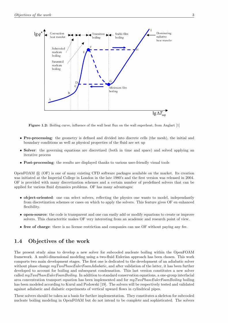
1.2 Boiling curve, influence of the wall heat flux on the wall superheat, from Anglart [1] . . . . . 3
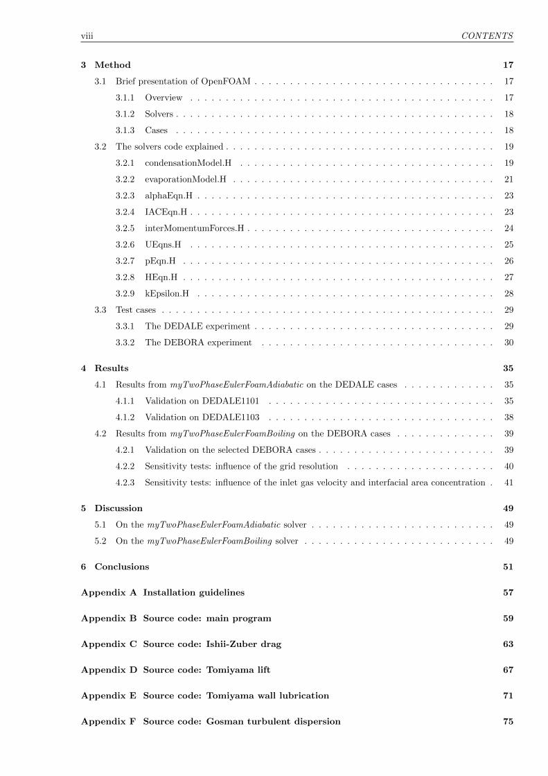
2.1 Influence of the bubble diameter on the Tomiyama lift coefficient for water at atmosphericpressure . . . . . . . . . . . . . . . . . . . . . . . . . . . . . . . . . . . . . . . . . . . . . . . . 8
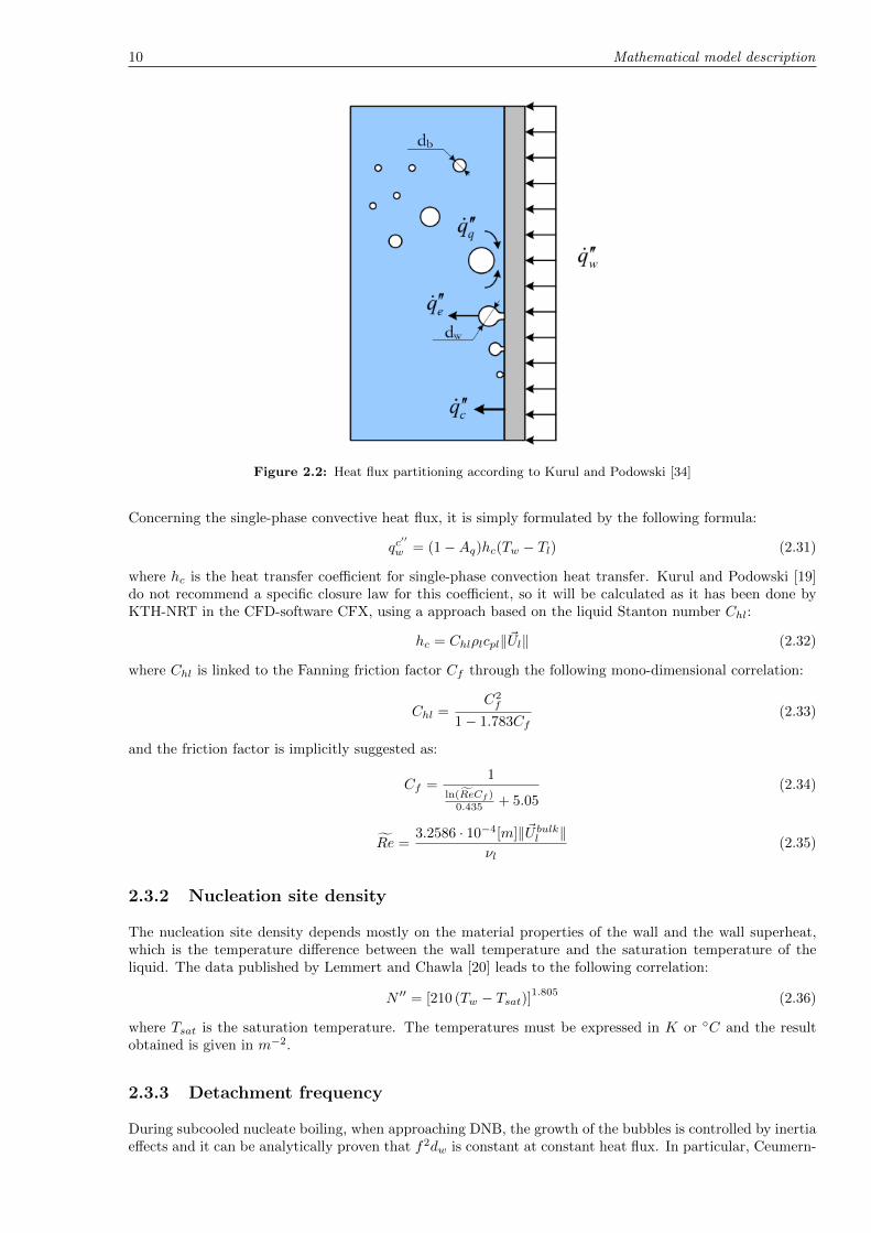
2.2 Heat flux partitioning according to Kurul and Podowski [34] . . . . . . . . . . . . . . . . . . . 10
2.3 Different behaviors occuring in the near-wall region [29] . . . . . . . . . . . . . . . . . . . . . 15
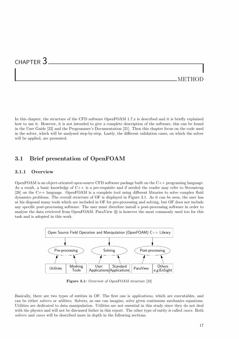
3.1 Overview of OpenFOAM structure [22] . . . . . . . . . . . . . . . . . . . . . . . . . . . . . . . 17
3.2 Directory structure for a solver [22] . . . . . . . . . . . . . . . . . . . . . . . . . . . . . . . . . 18
3.3 Graphical representation of the solution procedure adopted for myTwoPhaseEulerFoamBoiling(inspired from Thiele [30]) . . . . . . . . . . . . . . . . . . . . . . . . . . . . . . . . . . . . . . 20
3.4 Zoom on the grid used for the DEDALE simulations . . . . . . . . . . . . . . . . . . . . . . . 30
4.1 Comparison for DEDALE1101 between the results obtained in OpenFOAM with myTwoPhaseEuler-FoamAdiabatic, the experimental data and the results obtained by Yao and Morel with CATHARE 36
4.1 (continued) . . . . . . . . . . . . . . . . . . . . . . . . . . . . . . . . . . . . . . . . . . . . . . 37
4.2 3D view of DEDALE1101 when the Hibiki and Ishii models are selected . . . . . . . . . . . . 37
4.3 3D view of DEDALE1101 when the Yao and Morel models are selected . . . . . . . . . . . . . 38
4.4 Comparison for DEDALE1103 between the results obtained in OpenFOAM with myTwoPhaseEuler-FoamAdiabatic, the experimental data and the results obtained by Yao and Morel with CATHARE 38
4.4 (continued) . . . . . . . . . . . . . . . . . . . . . . . . . . . . . . . . . . . . . . . . . . . . . . 39
4.5 Comparison of the void fraction profiles at the end of the heated section between the resultsobtained in OpenFOAM with myTwoPhaseEulerFoamBoiling, the experimental data and theresults obtained by Yao and Morel with CATHARE for the selected DEBORA cases . . . . . 40
4.6 3D view of the liquid subcooling for the DEB5 case when the Yao and Morel model is used . 41
4.7 Comparison of the liquid temperature profiles at the end of the heated section between theresults obtained in OpenFOAM with myTwoPhaseEulerFoamBoiling, the experimental dataand the results obtained by Yao and Morel with CATHARE for the selected DEBORA cases 42
4.8 Comparison of the bubble diameter profiles at the end of the heated section between the resultsobtained in OpenFOAM with myTwoPhaseEulerFoamBoiling, the experimental data and theresults obtained by Yao and Morel with CATHARE for the selected DEBORA cases . . . . . 43
xiii
xiv List of Figures
4.9 Comparison of the interfacial area concentration profiles at the end of the heated sectionbetween the results obtained in OpenFOAM with myTwoPhaseEulerFoamBoiling, the exper-imental data and the results obtained by Yao and Morel with CATHARE for the selectedDEBORA cases . . . . . . . . . . . . . . . . . . . . . . . . . . . . . . . . . . . . . . . . . . . . 44
4.10 Comparison of the results obtained from myTwoPhaseEulerFoamBoiling at the end of theheated section for DEB5 with variying number of radial cells for the grid . . . . . . . . . . . . 45
4.11 Map of the field A′′′
w introducing a grid-dependency in the solvers . . . . . . . . . . . . . . . . 45
4.12 Comparison of the results obtained from myTwoPhaseEulerFoamBoiling at the end of theheated section for DEB5 with varying inlet gas velocity . . . . . . . . . . . . . . . . . . . . . 46
4.13 Comparison of the results obtained from myTwoPhaseEulerFoamBoiling at the end of theheated section for DEB5 with varying inlet interfacial area concentration . . . . . . . . . . . . 47
LIST OF TABLES
3.1 Transport properties of water and air in the DEDALE experiment . . . . . . . . . . . . . . . 29
3.2 DEDALE1101 and DEDALE1103 measured inlet conditions . . . . . . . . . . . . . . . . . . . 30
3.3 Initial and boundary conditions applied in OpenFOAM for DEDALE1101 . . . . . . . . . . . 30
3.4 Initial and boundary conditions applied in OpenFOAM for DEDALE1103 . . . . . . . . . . . 31
3.5 Properties of Inconel 600 used as pipe material in the DEBORA experiment . . . . . . . . . . 31
3.6 DEBORA selected cases and their experimental conditions . . . . . . . . . . . . . . . . . . . . 31
3.7 Transport properties of R12 in the selected DEBORA cases . . . . . . . . . . . . . . . . . . . 32
3.8 Initial and boundary conditions used in OpenFOAM for DEB5 . . . . . . . . . . . . . . . . . 32
3.9 Initial and boundary conditions used in OpenFOAM for DEB6 . . . . . . . . . . . . . . . . . 32
3.10 Initial and boundary conditions used in OpenFOAM for DEB10 . . . . . . . . . . . . . . . . . 32
3.11 Initial and boundary conditions used in OpenFOAM for DEB13 . . . . . . . . . . . . . . . . . 33
xv

xvi List of Tables
CHAPTER 1
INTRODUCTION
1.1 Background
The increasing world population requires to augment the global energy production. That has become oneof the biggest challenges in today’s society. In the context of fossil fuel shortage and global warming, theneed of sustainable, economical and safe technology has arisen. Renewable technologies such as wind power,photovoltaic cells or geothermal energy for example are of interest but some of them have to be furtherdeveloped. Nuclear power appears to be one of the most mature solutions in order to fulfill the abovecriteria.
Even though nuclear power sometimes still faces the public opinion’s reluctancy, most countries have admittedthat it will represent an important share also in tomorrow’s energy supply and they want to take part to whatis by some experts called “the nuclear renaissance ”. For instance, Sweden revised a previous law forbiddingnew build and a planned complete phase-out by 2010 and authorized the replacement of current reactorswith new reactors.
Among the existing types of reactors, Light Water Reactors (LWR) are the most commonly used, particularlyBoiling Water Reactors (BWR) and Pressurized Water Reactors (PWR). A basic knowledge concerning thesedesigns is a pre-requisite for this work but out of purpose in this report.
1.2 Subcooled nucleate boiling
Convective boiling in vertical heated channels has many industrial applications, including the core of LWRwhere heat is supplied by the nuclear reactions in the fuel. This is a very complex phenomenon which canbe divided into several regimes, depending on the local flow conditions, as shown in Figure 1.1. In the caseof a LWR, where water is subcooled at the inlet,the first stage in the boiling process is called subcoolednucleate boiling. Before subcooled nucleate boiling occurs, the heat transfer is governed by single-phaseforced convection. Subcooled nucleate boiling designates the evaporation of liquid in micro-cavities adjacentto the heated wall, also called nucleation sites, while the bulk liquid remains subcooled. When the walltemperature exceeds sufficiently the local saturation temperature, liquid evaporates and bubbles are formedat the nucleation sites. They grow until they reach a critical size and then detach from the heated wall.The bubbles migrate to the bulk of the fluid, which is subcooled, and condensate, heating the liquid phase.Subcooled boiling is said to be partial if the nucleation sites cover only a part of the heated wall. As thewall temperature increases, the area where single-phase convection occurs decreases and the area coveredby nucleation sites increases. When nucleation sites cover the whole surface, the regime is said to be fully-developed.
Modeling of subcooled nucleate boiling is a first attempt towards handling simulations of the boiling crisis,also known as Critical Heat Flux (CHF). At a heat flux equal to the CHF, there is a very sudden deteriorationof the heat transfer coefficient, leading to a sharp increase of the wall temperature since the heat flux imposedby fission reactions in the fuel remains unchanged. Therefore, the fuel rods structure may be damaged andradioactive material may be released to the primary system, which constitutes a serious infringement to the
1

2 Introduction
Figure 1.1: Flow patterns and heat transfer regimes in a heated channel, from Anglart [1]
defense-in-depth principle. At low thermodynamic equilibrium qualities, which is the in a PWR core or thelower part of a BWR core, the CHF occurs when the boiling mechanism evolves from nucleate boiling to filmboiling which is referred to as Departure from Nucleate Boiling (DNB), and represented by the point C inFigure 1.2. DNB sets an upper limit to the power that can be generated by the fuel.
In the case of PWR, even if this limit seems of no concern during normal operation, it is essential to ensurethat safety margins will also be respected in case of transients, incidents or accidents. Indeed, subcooledboiling can even occur in the higher part of a PWR core, and it would generate a lithium borate depositionwhich affects significantly the power distribution. This phenomenon is called axial offset anomaly (AOA). Thenuclear safety analysis of BWR is also influenced by the system reactivity. Subcooled nucleate boiling causesa highly inhomogeneous void fraction distribution in the axial direction (along the flow) since the channelis heated, but also in the cross-sectional direction due to the migration of steam bubbles. The presence ofbubbles and their distribution induces a non-negligible reactivity feedback. Consequently, it is crucial to beable to predict the void fraction distribution if one wants to couple thermal-hydraulics and neutronics. Thecodes used today for this purpose are still old system level codes with a quasi one-dimensional representationof the flow and heat transfer in the core. Clearly there is a need for advanced models of the complex physics.
1.3 Computational fluid dynamics (CFD)
Reproducing the flow conditions of a power plant in an experimental facility is very difficult and expensive.The development of Computational Fluid Dynamics (CFD) together with the evolution of modern powerfulcomputers the last decades has been a huge breakthrough within the industrial community. One can nowadayssimulate many (but not all!) non-trivial fluid dynamics problems through the modeling of heat transfer,turbulence or chemical reactions at a varying degree of accuracy. Still, such models always need to bevalidated against experimental data. Any CFD software consists of three parts :
Objectives of the work 3
Figure 1.2: Boiling curve, influence of the wall heat flux on the wall superheat, from Anglart [1]
• Pre-processing: the geometry is defined and divided into discrete cells (the mesh), the initial andboundary conditions as well as physical properties of the fluid are set up
• Solver: the governing equations are discretized (both in time and space) and solved applying aniterative process
• Post-processing: the results are displayed thanks to various user-friendly visual tools
OpenFOAM R© (OF) is one of many existing CFD software packages available on the market. Its creationwas initiated at the Imperial College in London in the late 1980’s and the first version was released in 2004.OF is provided with many discretization schemes and a certain number of predefined solvers that can beapplied for various fluid dynamics problems. OF has many advantages:
• object-oriented: one can select solvers, reflecting the physics one wants to model, independantlyfrom discretization schemes or cases on which to apply the solvers. This feature gives OF en enhancedflexibility.
• open-source: the code is transparent and one can easily add or modify equations to create or improvesolvers. This characteritic makes OF very interesting from an academic and research point of view.
• free of charge: there is no license restriction and companies can use OF without paying any fee.
1.4 Objectives of the work
The present study aims to develop a new solver for subcooled nucleate boiling within the OpenFOAMframework. A multi-dimensional modeling using a two-fluid Eulerian approach has been chosen. This workcomports two main development stages. The first one is dedicated to the development of an adiabatic solverwithout phase change myTwoPhaseEulerFoamAdiabatic, and after validation of the latter, it has been furtherdeveloped to account for boiling and subsequent condensation. This last version constitutes a new solvercalled myTwoPhaseEulerFoamBoiling. In addition to standard conservation equations, a one-group interfacialarea concentration transport equation has been implemented and for myTwoPhaseEulerFoamBoiling boilinghas been modeled according to Kurul and Podowski [19]. The solvers will be respectively tested and validatedagainst adiabatic and diabatic experiments of vertical upward flows in cylindrical pipes.
These solvers should be taken as a basis for further implementation. They constitutes a skeleton for subcoolednucleate boiling modeling in OpenFOAM but do not intend to be complete and sophisticated. The solvers
4 Introduction
are based on several assumptions, notably of incompressible phases, saturated gas phase, sphericalbubbles and no bubble-sliding. The closure relations present here, even if widely used in many softwarepackages, remain perfectible. But since OF is an open-source code, more complex and accurate models couldbe easily implemented at a later stage.
Regarding the structure of this report, Chapter 2 describes the mathematical model. Chapter 3 presentsbriefly how OF works and describes its structure and then finally the code is described as well as the detailsof the tested cases. Chapter 4 deals with the results and the validation of the solvers. In Chapter 5, adiscussion about possible future improvements is conducted. Last, in Chapter 5, the conclusions of this workare presented.
CHAPTER 2
MATHEMATICAL MODEL DESCRIPTION
This chapter is dedicated to a thorough description of the equations used in the solver. It begins with generalconservation equations valid for a two-phase Eulerian modeling, and continues with the successive additionalequations neccesary for the closure of the mathematical system of equations.
2.1 Governing flow equations
The code solves successively the different conservation equations (mass, momentum, energy), assuming in-compressibility of each of the phases. In this study, the continuous phase is liquid and the dispersed phaseis gaseous. The continuity equation can be written as:
∂αk∂t
+∇ ·(αk ~Uk
)=
Γki − Γikρk
(2.1)
where k denotes the phase and can be either l or g (liquid or gas) and i is the non-k phase. α, ρ and ~Urepresent the phase volume fraction, density and velocity respectively. The notation Γgl corresponds to theevaporation rate per unit volume, which within the scope of this study is due to nucleation at the wall, whereasΓlg is the condensation rate per unit volume, which is the only possible phase change at a phase interfacesince water remains subcooled and gas is saturated. This equation may be surprising because physically,condensation and evaporation can not occur at the exact same location. But in numerical calculations, it ispossible to have a near-wall cell which contains the two phases and in which could occur both condensationof the gas and evaporation of a part of the liquid phase.
One can also observe that it is not required to solve the continuity equation for both phases. It is sufficientto solve one of them, for example for the gas phase, and calculate the liquid fraction according to:
αl = 1− α (2.2)
where α = αg.
The momentum equation for phase k is given by:
∂αk ~Uk∂t
+∇ ·(αk ~Uk ~Uk
)= −∇ ·
(αk
(¯Rk + ¯R
t
k
))− αkρk
~∇p+ αk~g +~Mk
ρk+
Γki~Ui − Γik ~Ukρk
(2.3)
In Eq.2.3, the first term of the right hand side (RHS) is the combined (or effective) viscous and Reynolds(or so-called turbulent) stress. The second term of the RHS corresponds to the pressure drop in the channel.The third term of the RHS is gravity. The fourth term is the interfacial force per unit volume and will be theobject of a specific modeling. Finally, the last term represents the gain or loss of momentum due to phasechange. Incidentally, the latter has been seen too many times wrongly derived in the litterature in the formof various extravagant combinations of phase change rates and velocities.
5
6 Mathematical model description
According to Boussinesq [6], the turbulent stress tensor is analogous to that of Newtonian fluids and theresulting effective stress appears as a function of fluid properties and velocity:
¯Reffk = ¯Rk + ¯Rt
k = −(νk + νtk
)(∇~Uk +
(∇~Uk
)T− 2
3¯I∇ · ~Uk
)+
2
3¯Ikk (2.4)
where the identity tensor is identified as ¯I. kk designates the turbulent kinetic energy of phase k and νt itsturbulent kinematic viscosity. The calculation of turbulent parameters will be explained later.
The last conservation equation concerns energy. As mentioned previously, one of the assumptions is thatthe gas is always at saturated conditions. It would be irrelevant to solve an energy equation for the gaseousphase. Only one energy equation is required for the liquid phase. In comparison with heat flux densitiesconsidered, potential and kinetic energies of the interface can be neglected. Also, for bubbly two-phase flows,the only possible heat transfer from the gas to the liquid is by condensation. These assumptions are justifiedby Kurul and Podowski [19]. Then, the energy conservation equation written in terms of specific enthalpytakes the following form:
∂ ((1− α) il)
∂t+∇·
((1− α) il ~Ul
)= − 1
ρl∇·[(1− α)
(~ql + ~qtl
)]+
(1− α)
ρl
Dp
Dt+
Γlgig,sat − Γglilρl
+q′′
wA′′′
w
ρl(2.5)
where ~ql and ~qtl denote respectively the molecular and turbulent heat fluxes inside phase l. Here, the notationDDt represents the total derivative. The third term is due to phase change and the last one represents the
heat from the wall where q′′
w is the wall heat flux density and A′′′
w refers to the contact area with the wall perunit volume.
Now, if one uses Fourier’s law of conduction inside phase l, the molecular heat flux can be tramsformed to:
~ql = − λlcpl
~∇il (2.6)
where λ and cp are the thermal conductivity and the specific heat respectively.
A similar expression can be written for the turbulent energy exchange if one uses a mixing length model :
~qtl = − λtl
cpl~∇il (2.7)
where λt is the turbulent thermal conductivity obtained as:
λtl =cplν
tl
ρlPrtl(2.8)
where Prtl is the turbulent Prandtl number of phase l. There are several empirical correlations and analyticalrelations to determine it [19], [17], but it is always in the same range in the frame of this work, slightly below1. A constant value of 0.9 has been chosen for Prtl .
2.2 Interfacial forces
The interfacial forces acting on a bubble are caused by the liquid which surrounds it. So, in agreement withthe third of Newton’s law of motion, it can be written:
~Mg = − ~Ml (2.9)
It is very important to select adequate models describing this force. Very often, this force is assumed to bethe sum of different contributions, each one of them corresponding to a separate physical phenomenon:
~Mg = ~MDg + ~ML
g + ~MWLg + ~MTD
g + ~MVMg (2.10)
2.2.1 Drag force
The first term ~MDg is the drag force. This force represents the resistance opposed to the motion of a bubble
in the fluid. Its direction is therefore the opposite of the bubble’s relative velocity. The drag depends, as one
Interfacial forces 7
could expect, on the bubble’s shape and size. Several formulations exist but the Ishii-Zuber correlation [2]has been chosen here, since it is valid for densely distributed fluid particles, such as bubbles:
~MDg = −3
4
CDDS
ρlα‖~Ug − ~Ul‖(~Ug − ~Ul
)(2.11)
where DS is the Sauter diameter, equal to the actual bubble diameter since bubbles are assumed to besphericle within this work, and CD defined as:
CD = max
(24
1 + 0.15Re0.687bm
Rebm, 0.44
)(2.12)
Rebm =ρl‖~Ug − ~Ul‖DS
µm(2.13)
µm = µl
(1− α
αmax
)−2.5αmaxµ∗(2.14)
Here, αmax is the void fraction at maximum packing equal to 0.52 and µ∗ is the dimensionless dynamicalviscosity:
µ∗ =µg + 0.4µlµg + µl
(2.15)
The Ishii-Zuber drag model presented above is valid for densely distributed sphericle fluid particles, with avoid fraction α < 0.52 and at the condition that 0.2 < Reb < 100000
2.2.2 Lift force
The second term ~MLg is the lift force which must be treated carefully since it plays an important role and
has a large effect on the radial distribution of bubbles. The following general formulation was proposed byDrew and Lahey ([10]):
~MLg = CLρlα
(~Ug − ~Ul
)∧(∇∧ ~Ul
)(2.16)
where CL is the lift coefficient which has been investigated by many authors. Here the Tomiyama model waschosen:
CL =
min [0.288 tanh (0.121Reb) , f (Eod)] if Eod < 4f (Eod) if 4 ≤ Eod ≤ 10−0.27 if Eod > 10
(2.17)
f (Eod) = 0.001509Eo3d − 0.0159Eo2d − 0.0204Eod + 0.474 (2.18)
The involved quantities are the bubble Reynolds number Reb and a modified Eotvos number (describing theratio between buoyancy forces and those from surface tension ) Eod for the maximum horizontal dimensionof the bubble dh, that is calculated using a correlation developed by Wellek et al. [36]:
Reb =‖~Ug − ~Ul‖DS
νl(2.19)
dh = Ds
(1 + 0.163Eo0.757
)1/3(2.20)
Eo =g (ρl − ρg)D2
s
σ(2.21)
Eod =g (ρl − ρg) d2h
σ(2.22)
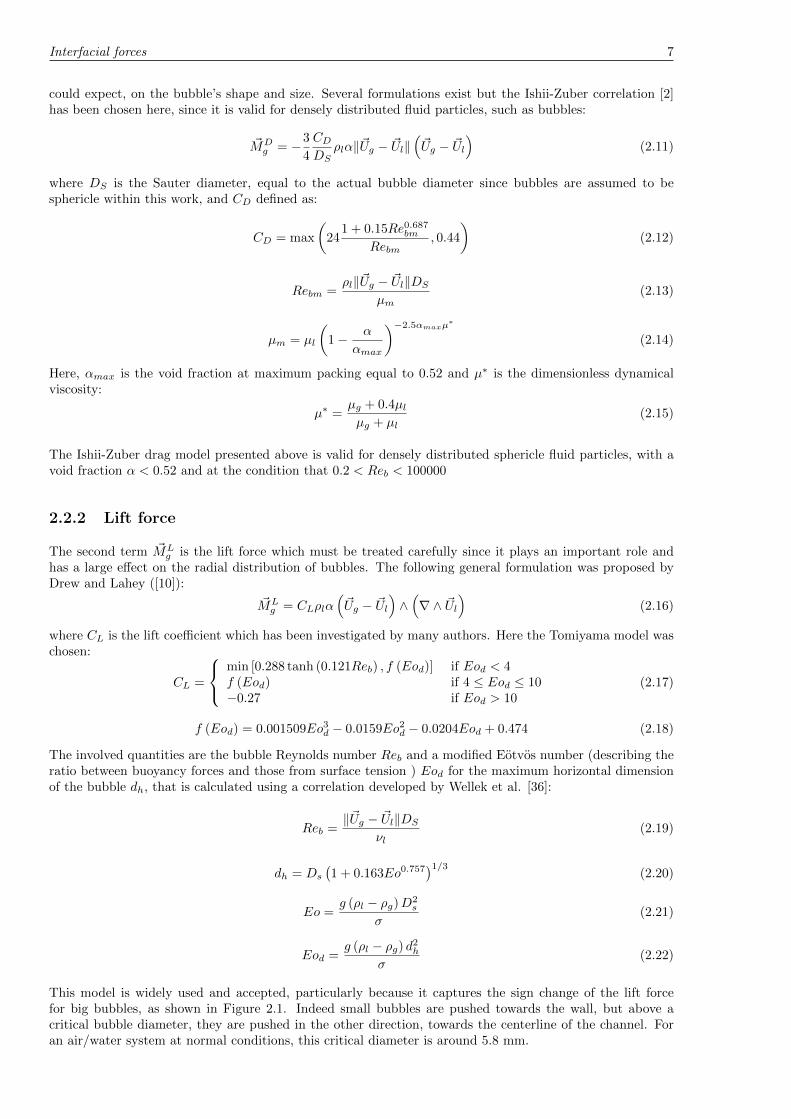
This model is widely used and accepted, particularly because it captures the sign change of the lift forcefor big bubbles, as shown in Figure 2.1. Indeed small bubbles are pushed towards the wall, but above acritical bubble diameter, they are pushed in the other direction, towards the centerline of the channel. Foran air/water system at normal conditions, this critical diameter is around 5.8 mm.

8 Mathematical model description
0 0.001 0.002 0.003 0.004 0.005 0.006 0.007 0.008 0.009 0.01−0.4
−0.3
−0.2
−0.1
0
0.1
0.2
0.3
Bubble Diameter [m]
Lift
Co
eff
icie
nt
CL
Figure 2.1: Influence of the bubble diameter on the Tomiyama lift coefficient for water at atmospheric pressure
2.2.3 Wall lubrication force
Furthermore, experiments on adiabatic two-phase flow showed evidence of the existence of a repulsive forcepushing bubbles away from the wall. If bubbles were concentrated close to the wall, they were never adjacentto it. The force which is responsible for this wall peaking phenomenon is the so-called wall lubrication force,denoted by ~MW
g in Eq. 2.10. Antal [3] was the first to derive an analytical expression of the wall lubricationforce. Tomiyama improved this model for pipe geometries [33], using a correlation whose constants are basedon glycerol/air flow experiments. However the model turned out to be valid for other two-phase systems suchas air/water:
~MWLg =
1
2CWLρlαDS
(1
x2− 1
(D − x)2
)‖(~Ug − ~Ul) · ~y‖2~nr (2.23)
CWL =
0.47 if Eo < 1e−0.933Eo+0.179 if 1 ≤ Eo ≤ 50.00599Eo− 0.0187 if 5 < Eo < 330.179 if 33 < Eo
(2.24)
where CW is the wall lubrication force coefficient, D the pipe diameter, x the distance to the wall, ~y theaxial direction and ~nr the normal to the wall pointing towards the fluid. This model is however geometry-dependent and limited to pipes. Frank [11] developed a more general formulation based on Tomiyama walllubrication force coefficient and a damping function independent of the geometry, but this improved modelis not considered in the solver.
2.2.4 Turbulent dispersion force
The fourth component in in Eq. 2.10 is the turbulent dispersion force, referred to as ~MTDg . The turbulent
dispersion force accounts for the turbulent fluctuations of liquid velocity and the effect that has on the gasbubbles. Gosman et al. [12] proposed the following relation:
~MTDg = −3
4
CDDS
νtlPrtl
ρl‖(~Ug − ~Ul)‖ ~∇α (2.25)
The turbulent dispersion plays a major role in the radial void fraction distribution. For small bubbles inadiabatic flow, one can observe the so-called wall-peaking phenomenon where most of the bubbles agglomerateclose to the wall but not in contact with it. The turbulent dispersion force strongly influences the sharpness

Boiling model 9
of this void wall peak, meaning its extent in the x-direction. For big bubbles whose lift force push themtowards the centerline, the turbulent dispersion is the only force to limit the so-called core voiding whichdesignates the agglomeration of bubbles around the centerline of the channel.
2.2.5 Virtual mass force
Finally the last force component in Eq. 2.10 is the virtual mass force, or added mass force, ~MVMg . The
virtual mass force takes its origin from the relative acceleration of one phase to the other. Therefore, thisforce is often neglected when running steady state calculations. It is considered in this study even though itscontribution vanishes fast. According to Zuber ([40]), the virtual mass force for spherical bubbles is equalto:
~MVMg = −1
2ρl
1 + 2α
1− αα
(D~UgDt− D~Ul
Dt
)(2.26)
This force has been implemented in our solver so that the user can possibly use it. However, it has beenfound to be the origin of many instabilities and has therefore been neglected in Eq.2.10.
2.3 Boiling model
2.3.1 Wall heat flux partitioning
Over the past 50 years, different subcooled nucleate boiling models have been developed. On the one hand,one-dimensional empirical correlations, based on experiments, connect the wall heat flux and the wall super-heat as a function of global parameters like pressure. One can for example refer to Jens-Lottes [16] or Thomet al. [31] correlations. Yet, these approaches do not lend themselves to CFD applications since they do notallow the calculation local parameters such as the evaporation rate and the bubble departure diameter.
On the other hand, mechanistic models based on local parameters (temperature, void fraction or for exampleturbulence intensity) could be used without any difficulty in CFD. One of them was presented by Kurul andPodowki [19] and it is the model applied in this solver. The basic idea in the model is that the heat transferoriginates from three different mechanisms between the heated wall and the liquid phase:
q′′
w = qc′′
w + qe′′
w + qq′′
w (2.27)
where qc′′
w , qe′′
w and qq′′
w denote respectively single-phase convective heat flux density, evaporation heat fluxdensity and quenching heat flux density. A schematic view of the boiling process is shown in Figure 2.2. Atthe heated wall, bubbles are formed at the nucleation sites due to evaporation of liquid at the wall and onetherefore assumes that part of the wall heat flux density is directly used to transform the liquid into vapor.Bubbles grow and reach a critical size at which they detach from the wall. Once a bubble leaves the wall,the volume previously occupied by it is filled with cooler liquid, which will receive heat from the wall. Theheat transfer to this cooler liquid is called quenching. The ratio of the wall influenced by quenching Aq isthus closely depending on the evaporation and the bubble lift-off size. Finally, the rest of the wall 1−Aq isgoverned by single-phase convection.
The evaporation heat flux can easily be calculated as a function of other key parameters: the nucleation sitedensity N
′′, the detachment frequency f and the bubble detachment (or departure or lift-off) diameter dw.
It is given by:
qe′′
w =π
6d3wρvfN
′′(ig,sat − il) (2.28)
DelValle and Kenning [9] derived an analytical solution for the quenching heat flux, assuming a transientheat transfer in a liquid cylinder with a diameter equal to dw. They showed, if one makes the hypothesisthat the growth time is much shorter than the time between two subsequent nucleations, that:
Aq = πN ′′d2w (2.29)
qq′′
w = Aq2λl(Tw − Tl)√
πf
λlρlcpl
(2.30)
10 Mathematical model description
Figure 2.2: Heat flux partitioning according to Kurul and Podowski [34]
Concerning the single-phase convective heat flux, it is simply formulated by the following formula:
qc′′
w = (1−Aq)hc(Tw − Tl) (2.31)
where hc is the heat transfer coefficient for single-phase convection heat transfer. Kurul and Podowski [19]do not recommend a specific closure law for this coefficient, so it will be calculated as it has been done byKTH-NRT in the CFD-software CFX, using a approach based on the liquid Stanton number Chl:
hc = Chlρlcpl‖~Ul‖ (2.32)
where Chl is linked to the Fanning friction factor Cf through the following mono-dimensional correlation:
Chl =C2f
1− 1.783Cf(2.33)
and the friction factor is implicitly suggested as:
Cf =1
ln(ReCf )0.435 + 5.05
(2.34)
Re =3.2586 · 10−4[m]‖~U bulkl ‖
νl(2.35)
2.3.2 Nucleation site density
The nucleation site density depends mostly on the material properties of the wall and the wall superheat,which is the temperature difference between the wall temperature and the saturation temperature of theliquid. The data published by Lemmert and Chawla [20] leads to the following correlation:
N ′′ = [210 (Tw − Tsat)]1.805 (2.36)
where Tsat is the saturation temperature. The temperatures must be expressed in K or ◦C and the resultobtained is given in m−2.
2.3.3 Detachment frequency
During subcooled nucleate boiling, when approaching DNB, the growth of the bubbles is controlled by inertiaeffects and it can be analytically proven that f2dw is constant at constant heat flux. In particular, Ceumern-

Boiling model 11
Lindenstjerna [7] came to the result:
f =
√3
4
(ρl − ρg)gρldw
(2.37)
2.3.4 Bubble detachment diameter
The determination of the bubble detachment diameter is doubtlessly a key characteristic in modeling ofsubcooled nucleate boiling. Performing an energy balance for a bubble growing at a heated surface, andfitting some constants to experimental water data, Unal [35] expressed the bubble detachment diameter as:
dw =2.42 · 10−5p0.705a√
bΦ(2.38)
where:
a =(Tw − Tl)λlγ
2ρgifg√π λlρlcpl
(2.39)
where ifg is the latent heat and:
γ =
√λwρwcpwλlρlcpl
(2.40)
b =Tsat − Tl
2(
1− ρgρl
) (2.41)
Φ =
{ (vbulkl
0.61
)0.47if vbulkl > 0.61
1 if vbulkl < 0.61(2.42)
and vbulkl represents the axial component of the liquid phase in the bulk. In the Unal correlation, allparameters must be given in the S.I, meaning that the pressure must be given in Pa, the velocity in m/sand the returned result for the bubble diameter is expressed in m.
But specific care must be taken while using this correlation since its range of validity is the following:0.1 < p < 17.7Mpa0.47 < qw < 10.64MW/m2
0.08 < vbulkl < 9.15m/s3.0 < Tsat − Tl < 86K0.08 < dw < 1.24mm
(2.43)
For low subcooling, other correlations must be used. At very low subcooling, below 2K, one must switchto the Tolubinsky and Kostanchuk expression [32] which predicts an exponential decrease of the detachmentdiameter with the subcooling:
dw = 1.4 · 10−3 exp
(−Tsat − Tl
45
)(2.44)
Here again, all units are those from the S.I.
If the subcooling is between 2 K and 3 K, then the detachment diamater is calculated using a linear inter-polation. In order to be able to use the same correlation for the whole range of subcooling, Boree et al.[5] modified the parameter b of the Unal correlation and defined it as a function of the Stanton number.However this improvement has not been taken into account in the present solver. It must also be recalledthat the Unal correlation was established for water/vapor system only, but Manon [24] demonstrated thatthe results given by this correlation were in agreement with the experiments even when Freon 12 (R12) isused as coolant.
12 Mathematical model description
2.3.5 Wall superheat
Having a look a the boiling model that has been explained in the previous subsections, all variables onlydepend on physical properties and local parameters (velocity, temperature for both phases, pressure) whichcan be retrieved from the CFD software and the wall superheat, which is so far the only unknown in thisboiling model.
The wall superheat is solved using a Newton-type iterative method. An initial guess is made for the wallsuperheat Tw − Tsat and the different heat flux contributions are calculated, then the wall superheat isadjusted if Eq.2.27 is not fulfilled.
2.4 Interfacial mass transfer
2.4.1 Evaporation rate
Evaporation occurs at the heated wall only and can be deduced easily since the evaporation heat fluxcontribution is known from the previous section. The evaporation rate per unit volume is expressed as:
Γgl =qe′′
w
ig,sat − ilA′′′
w =π
6d3wρvfN
′′A′′′
w (2.45)
2.4.2 Condensation rate
Once bubbles are created and moves towards the centerline, they are surrounded by subcooled water andcondense. In the case of subcooled nucleate boiling, condensation is indeed the only possible physical phasechange at the interface for cells which are not in contact with the wall. The interfacial mass transfer relatedto condensation of vapor bubbles in the bulk coolant is found as:
Γlg =hli(Tsat − Tl)ai
ifg(2.46)
where ai represents the interfacial area concentration and hli the heat transfer coefficient for condensationat the interface described by Wolfert et al. [37], assuming that bubbles are at saturated conditions as:
hli = ρlcpl
√π
4
‖~Ug − ~Ul‖DS
λlρlcpl
1
1 + λtl/λl(2.47)
2.5 Interfacial area concentration transport equation
The interfacial area concentration (IAC) corresponds to the area of the gas bubbles per unit volume. Forspherical bubbles, due to geometrical reasons, it is directly proportional to the void fraction and inverselyproportional to the bubble diameter:
ai = 6α
DS(2.48)
The IAC is influenced by many different phenomena. It can increase or decrease due to sudden phase change(condensation in the bulk or nucleation at the wall). Coalescence and breakup mechanisms also affect theIAC. Coalescence consists of several bubbles joining together to form a larger bubble, decreasing the areafor the same volume of void so that the IAC decreases. This is provoked by collisions driven by turbulence.The opposite phenomenon is breakup of bubbles which results from the interaction between bubbles andturbulent eddies. In the case of breakup, one bubble splits into two or several smaller bubbles and the IACincreases as the consequence.
There is a spatial and temporal evolution of the IAC, which has to be described by an additional equation.Since most of the interfacial forces are functions of the bubble diameter, and indirectly of the IAC, this extraequation must be modeled accordingly. Yao and Morel ([39]) derived an analytical form:
∂ai∂t
+∇ ·(ai~Ug
)= −2
3
aiα
Γlg +36π
3
(α
ai
)2 (φCOn + φBKn
)+ πd2wφ
NUCn (2.49)
Turbulence modeling 13
where φCOn and φBKn are a bubble sink term by coalescence and a bubble source term by breakup respectivelyand φNUCn is the source term by nucleation at the wall, equal to:
φNUCn = fN′′A′′′
w (2.50)
Many people have investigated these parameters. Wu et al. [38] and Ishii and Kim [14] derived expressionsfor these two terms and also introduced another term in Eq.2.49 reflecting the wake entrainment, meaningthe acceleration of the following bubble in the wake of the preceding bubble. The Yao and Morel model [39]was chosen in the NEPTUNE code which has been implemented in the frame of a collaboration between themain french nuclear authorities and companies (CEA, Areva, EDF, IRSN). For a good description of thedifferences between the different models referred to here, see Delhaye [8]. In the present work, the Hibiki andIshii model [13] is considered as the standard model in the present solvers. According to Hibiki and Ishii,the coalescence and breakup terms are found to be:
φCOn = −ΓCα2ε
1/3l
D11/3S (αmax − α)
exp
(−KC
D11/3S ρ
1/2l ε
1/3l
σ1/2
)(2.51)
where: {ΓC = 0.005KC = 1.29
(2.52)
and,
φBKn = ΓBα(1− α)ε
1/3l
D11/3S (αmax − α)
exp
(−KB
σ
D5/3S ρlε
2/3l
)(2.53)
where: {ΓB = 0.007KB = 1.37
(2.54)
However, the Yao and Morel model has also been created and can be selected if required by the user instead ofthe standard Hibiki and Ishii formulation. Yao and Morel derived the following expressions for the coalescenceand breakup terms:
φCOn = −KC1α2ε
1/3l
D11/3S
1
α1/3max−α1/3
α1/3max
+KC2α√
WeWecr
exp
(−KC3
We
Wecr
)(2.55)
where: KC1 = 2.86KC2 = 1.922KC3 = 1.017Wecr = 1.24
(2.56)
and,
φBKn = KB1α (1− α) ε
1/3l
D11/3S
1
1 +KB2 (1− α)√
WeWecr
exp
(−WecrWe
)(2.57)
where: {KB1 = 1.6KB2 = 0.42
(2.58)
2.6 Turbulence modeling
2.6.1 Turbulence of the liquid phase
The effective viscosity of the liquid phase is the sum of a molecular and a turbulent viscosity.
νeffl = νl + νtl (2.59)
The turbulent behavior of the liquid phase is in turn decomposed in two different contributions:

14 Mathematical model description
• an inherent shear-induced turbulence modeled as a classical single-phase k − ε expression:
νt,k−εl = Cµk2lεl
(2.60)
where the typical value of the constant Cµ is 0.09
• a bubble-induced turbulence described by Sato et al. [27]:
νt,bl =1
2CµbDSα‖~Ug − ~Ul‖ (2.61)
where the value of the constant Cµb is 1.2.
To summarize, the turbulent viscosity of the liquid phase is given by:
νtl = Cµk2lεl
+1
2CµbDSα‖~Ug − ~Ul‖ (2.62)
2.6.2 Turbulence of the gas phase
The turbulence of the gas phase is assumed to be dependant on the liquid phase turbulence and a turbulenceresponce coefficient Ct, defined as the ratio of the root mean square values of dispersed phase velocityfluctuations to those of the continuous phase, given by:
Ct =U′
g
U′l
(2.63)
This approach described by Rusche [26] presents the advantage not to introduce any extra differential equa-tion. The effective viscosity of the gas phase is simply expressed as:
νeffg = νg + C2t ν
tl (2.64)
Various authors have derived expressions to calculate Ct as a function of local parameters such as the voidfraction, but in the present solvers, a constant value is set by the user. By default, the value used for thesimulations is set to zero, and no turbulence is affected to the gas phase.
2.6.3 Near-wall treatment: wall functions
It is well known that even for turbulent flows, there is very close to the wall a viscous sub-layer where theflow is quasi-laminar. Further away from the wall, in the outer parts of the near-wall region, the flow isturbulent. Between these two zones, there is a transition called the buffer region. The velocity profile andthe extent of the different regions is shown in Figure 2.3. It has to be pointed out that within the frame ofthis work, ~x and ~y denote respectively the wall normal direction and the axial direction.
Thus, if one wants to capture the behaviour of the velocity in CFD, the near-wall region needs a specificattention and must be treated carefully. One option is to refine the mesh in the vicinity of the wall so that thenear-wall region is resolved. But for flows at high Reynolds number, this solution can be very computationallyexpensive. Therefore, another approach is to model the flow based on wall functions as described below.
The k-equation is solved in the whole domain, even for near-wall cells, which is not the case for the ε-equation.Instead ε is found close to the wall from:
εl =C
3/4µ k
3/2l
κx(2.65)
where κ is the von Karman constant equal to 0.42.
Once k is known, it is possible to derive the dimensionless distance to the wall x+ from the relation:
x+ =C
1/4µ k
1/2l
νl· x (2.66)

Summary 15
Figure 2.3: Different behaviors occuring in the near-wall region [29]
Depending on the value which is obtained, one will know in which layer the near-wall cells are and how tohandle them. For x+ > 11.6, it is assumed that the flow is in the turbulent region. Then the shear-inducedturbulent viscosity of the liquid phase and the buoyant production term appearing in the k-ε equation are:
νt,k−εl = νl
(yκ
ln(Ex+)− 1
)(2.67)
Gt,k−εl =νt,k−εl ‖∂~Ul∂x ‖C
1/4µ k
1/2l
κx(2.68)
where E is a constant equal to 9.793.
On the opposite, if x+ < 11.6, viscous effects dominate (viscous sub-layer) and it is assumed that there is noshear-induced turbulence:
νt,k−εl = Gt,k−εl = 0 (2.69)
Updating the fields for near-wall cells as detailed previously will implicitly apply the standard law of the wallfor the velocity field of the liquid phase:{
U+ = x+ if x+ < 11.6U+ = 1
κ ln(Ex+) if x+ > 11.6(2.70)
2.7 Summary
The presented mathematical models contains 8 independent equations :
• 2 mass conservation equations for the liquid and gas phases
• 2 momentum conservation equations for the liquid and gas phases
• 1 energy conservation equation for the liquid phase
• 1 interfacial area concentration transport equation
• 2 additional partial derivative equations for the turbulence of the liquid phase
Using various closures laws, all the parameters appearing in these equations have been expressed as a functionof 8 independent variables:
• the void fraction α
• the gas velocity ~Ug

16 Mathematical model description
• the liquid velocity ~Ul
• the specific enthalpy of the liquid phase il
• the interfacial are concentration ai
• the turbulent kinetic energy of the liquid phase kl
• the turbulent dissipation rate of the liquid phase εl
• the pressure p
The mathematical system of equations is properly defined and can be solved numerically.
CHAPTER 3
METHOD
In this chapter, the structure of the CFD software OpenFOAM 1.7.x is described and it is briefly explainedhow to use it. However, it is not intended to give a complete description of the software, this can be foundin the User Guide [22] and the Programmer’s Documentation [21]. Then this chapter focus on the code usedin the solver, which will be analysed step-by-step. Lastly, the different validation cases, on which the solverwill be applied, are presented.
3.1 Brief presentation of OpenFOAM
3.1.1 Overview
OpenFOAM is an object-oriented open-source CFD software package built on the C++ programing language.As a result, a basic knowledge of C++ is a pre-requisite and if needed the reader may refer to Stroustrup[28] on the C++ language. OpenFOAM is a complete tool using different libraries to solve complex fluiddynamics problems. The overall structure of OF is displayed in Figure 3.1. As it can be seen, the user hasat his disposal many tools which are included in OF for pre-processing and solving, but OF does not includeany specific post-processing software. The user must therefore install a post-processing software in order toanalyse the data retrieved from OpenFOAM. ParaView R© is however the most commonly used too for thistask and is adopted in this work.
Figure 3.1: Overview of OpenFOAM structure [22]
Basically, there are two types of entities in OF. The first one is applications, which are executables, andcan be either solvers or utilities. Solvers, as one can imagine, solve given continuum mechanics equations.Utilities are dedicated to data manipulation. Utilities are not essential in this study since they do not dealwith the physics and will not be discussed futher in this report. The other type of entity is called cases. Bothsolvers and cases will be described more in depth in the following sections.
17

18 Method
3.1.2 Solvers
Each solver represents a specific continuum mechanics problem to solve in which the governing equations areimplemented. The source file of the solver must have the .C -extension and be placed, by convention, in afolder wearing the same name as the source file. This folder can also contain other files with the .H -extensionwhich are ”used” or referred to by the main source code. It is for example quite useful when the code islarge, since it allows to separate the main code into several parts, which is of huge interest while debuggingthe code. Files with the .H -extension can also designate an already existing class used in the main sourcecode. The last type of file included in the solver folder is another folder named Make which is essential forthe compilation. Make is composed of two files: files and options which incorporate paths to the differentfiles that must be compiled and the paths to the necessary libraries. For example, a solver called newAppcould have the following structure:
Figure 3.2: Directory structure for a solver [22]
As explained earlier, a solver contains the different equations to be solved. One of OpenFOAM’s strengths isits equation representation, whose syntax is realy similar to the mathematical one. Considering for examplethe following transport equation for a field T :
∂T
∂t+∇ ·
(T ~U)−∇ ·
(ν ~∇T
)= 0 (3.1)
would be written:
solve(
fvm::ddt(T)+ fvm::div(phi, T)- fvm::laplacian(nu, T)
);
After the physical problem is properly put into equations in the solver, the latter must be compiled. Thisprocess is done very easily. In the Linux environment, one has only to open a terminal, go to the solver’sdirectory and type in the command wmake. This will create the executable file that can be applied on cases.
3.1.3 Cases
If a solver contains the universal aspects of a physical problem, meaning the equations, a case on the contraryrefers to the specificities of a problem (geometry, physical properties, computational schemes, etc). A case isa folder that is based on three main directories : system, constant and 0.
The system directory usually contains three different files. The first file is controlDict and is used to set upfor example the starting time of the simulation, the write interval, the end time, the time step as well ascalculating the output data. The second file fvSchemes is for setting up the numerical discretisation schemeswhich are used for time and spatial derivatives. The third and last file is called fvSolution, it containsinformation associated with the solution procedure i.e. solvers to be used for the given equations, solutionalgorithm structure, relaxation and tolerances.
The constant directory is composed of one folder called polyMesh and several other files. The polyMeshfolder includes the definition of the geometry. How to create a geometry will not be described in details
The solvers code explained 19
here but the user may refer to [22]. Among the other files located in the constant, one finds for example thetransportProperties file (which contains mostly physical properties of the two phases, pressure and constants),the environmentalProperties (including the wall heat flux and wall material properties), the g file (in whichthe gravity field is defined), the interfacialProperties file (for setting up the models chosen for the interfacialforces) and the turbulenceProperties (where the turbulence model and the associated constants are defined).Of course, the number of files and their nature depends on the case since the required information variesfrom one application to another, but the files described here are those normally used in the two-phase flowsimulations considered here.
The 0 directory contains the initial and boundary conditions of all fields that have to be solved. There arefew pre-defined initial or boundary conditions in OF that are quite often sufficient in common applications.They are described in the OpenFOAM User Guide [22].
Then, in order to run an specific solver (which must have been compiled before) on a case in the Linuxenvironment, one has to open a terminal, go into the case folder and type the name of the compiled solver.This will run the code and additional directories containing the calculated fields will be created in the casedirectory. Their names are the time at which the results are written.
3.2 The solvers code explained
In this work, two different solvers have been implemented: one for adiabatic flows, myTwoPhaseEulerFoa-mAdiabatic, and one for heated flows, myTwoPhaseEulerFoamBoiling.
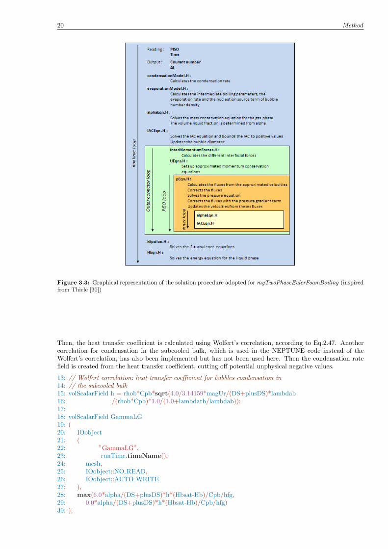
The solvers are improved versions of the twoPhaseEulerFoam solver which is already included in OF. Certainfiles have been removed because they were unnecessary for subcooled boiling, such as the kinetic theory model,but many others have been created or modified. For instance, the phaseModel class has been modified andmany other interfacial forces have been implemented in the interfacialModels class (not only drag models as itwas done so far). An energy equation written in terms of enthalpy has been introduced as well. The algorithmprocedure is the so-called Pressure-Implicit with Splitting of Operatos (PISO) which is adapted for transientcalculations. A graphical representation of the solution procedure used in myTwoPhaseEulerFoamBoilingcan be seen in Figure 3.3.
These two solvers that have been created have a similar structure. myTwoPhaseEulerFoamAdiabatic differsfrom myTwoPhaseEulerFoamBoiling only through the headers condensationModel.H, evaporationModel.Hand HEqn.H which are not present. The other headers are absolutely identical, except the fact that inmyTwoPhaseEulerFoamAdiabatic, the phase change terms have been removed from the equations.
As can be noticed from Figure 3.3, all equations are set up in different header files with the .H -extension.The code of each of these files constituting myTwoPhaseEulerFoamBoiling will be described shortly withinthe following subsections. The line numbers appearing to the left side correspond to the number of the linesin the source code files, as they appear in the appendices.
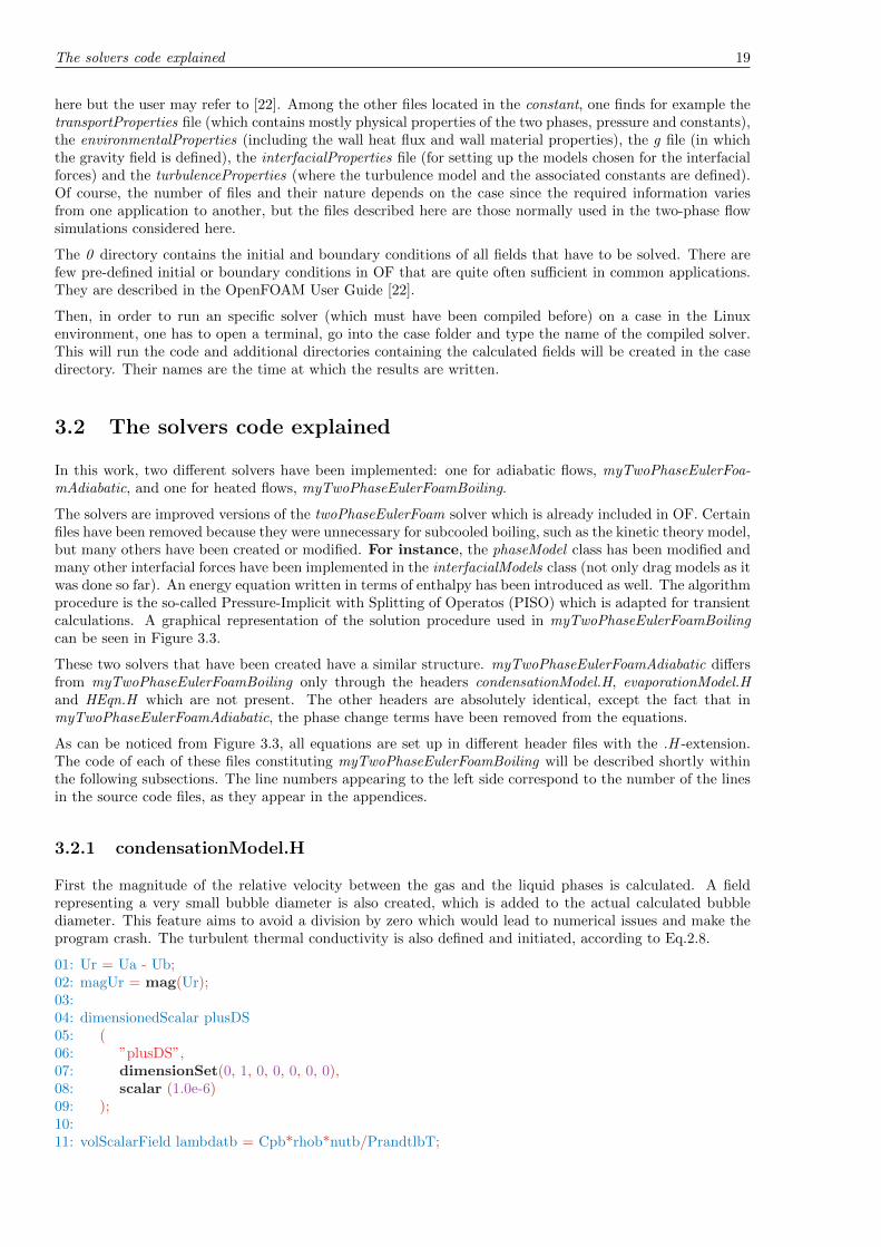
3.2.1 condensationModel.H
First the magnitude of the relative velocity between the gas and the liquid phases is calculated. A fieldrepresenting a very small bubble diameter is also created, which is added to the actual calculated bubblediameter. This feature aims to avoid a division by zero which would lead to numerical issues and make theprogram crash. The turbulent thermal conductivity is also defined and initiated, according to Eq.2.8.
01: Ur = Ua - Ub;02: magUr = mag(Ur);03:04: dimensionedScalar plusDS05: (06: ”plusDS”,07: dimensionSet(0, 1, 0, 0, 0, 0, 0),08: scalar (1.0e-6)09: );10:11: volScalarField lambdatb = Cpb*rhob*nutb/PrandtlbT;
20 Method
Figure 3.3: Graphical representation of the solution procedure adopted for myTwoPhaseEulerFoamBoiling (inspiredfrom Thiele [30])
Then, the heat transfer coefficient is calculated using Wolfert’s correlation, according to Eq.2.47. Anothercorrelation for condensation in the subcooled bulk, which is used in the NEPTUNE code instead of theWolfert’s correlation, has also been implemented but has not been used here. Then the condensation ratefield is created from the heat transfer coefficient, cutting off potential unphysical negative values.
13: // Wolfert correlation: heat transfer coefficient for bubbles condensation in14: // the subcooled bulk15: volScalarField h = rhob*Cpb*sqrt(4.0/3.14159*magUr/(DS+plusDS)*lambdab16: /(rhob*Cpb)*1.0/(1.0+lambdatb/lambdab));17:18: volScalarField GammaLG19: (20: IOobject21: (22: ”GammaLG”,23: runTime.timeName(),24: mesh,25: IOobject::NO READ,26: IOobject::AUTO WRITE27: ),28: max(6.0*alpha/(DS+plusDS)*h*(Hbsat-Hb)/Cpb/hfg,29: 0.0*alpha/(DS+plusDS)*h*(Hbsat-Hb)/Cpb/hfg)30: );

The solvers code explained 21
3.2.2 evaporationModel.H
The evaporationModel.H leads to the determination of the wall heat flux partition and the evaporation ratecan be calculated.
Even though all quantities are defined as volScalarField in the whole geometry, it is obvious that evaporationonly occurs in near-wall cells. Therefore, a first step is to localize them and also the cell located at the sameaxial position in the bulk. For simplicity’s sake, the bulk is assumed to be at the centerline. This is done inthe following lines:
348: forAll(thePatchItselfWall,iFace)349: {350:351: label iCell = thePatchItselfWall.faceCells()[iFace];352: vector iCellCentre = mesh.cellCentres()[iCell];353:354: //Point located at the center line but on the same axial position355: vector bulkPoint(0,iCellCentre.y(),iCellCentre.z());356: label bulkCell = mesh.findCell(bulkPoint);
Once the near-wall cells are localized, it is useful to calculate their dimensions. It is done in the followinglines:
358: // Needed to take the cell dimensions in order to check that the bubble are359: // are not too large for the mesh at the wall360: const cell & cc = mesh.cells()[iCell];361: labelList pLabels(cc.labels(ff));362: pointField pLocal(pLabels.size(), vector::zero);363:364: forAll (pLabels, pointi)365: {366: pLocal[pointi] = pp[pLabels[pointi]];367: }368:369: scalar xDim = Foam::max(pLocal & vector(1,0,0)) - Foam::min(pLocal & vector(1,0,0));370: scalar yDim = Foam::max(pLocal & vector(0,1,0)) - Foam::min(pLocal & vector(0,1,0));371: scalar zDim = Foam::max(pLocal & vector(0,0,1)) - Foam::min(pLocal & vector(0,0,1));372:
After that, an initial guess must be made for the wall superheat. This is done by assuming that the total heatflux density will be dedicated to single phase convection. However, the real heat transfer coefficient for singlephase convection is not know yet since it is calculated from the Kurul and Podowski partitioning. Therefore,the first step is to calculate the Fanning friction factor according to a given correlation, and from factorto derive the Stanton number according to another correlation. These correlations are those implementedin the Fortan code developed by KTH-NRT in CFX R©. The original Fortran code can be found in theappendix. Using the definition of the Stanton number, one can finally calculate the heat transfer coefficient.This procedure to calculate an initial guess of the wall superheat is implemented as:
376: for (int i=0; i<10; i++)377: {378: Cf[iCell] = 1.0/(Foam::log(Reyno.value()*Cf[iCell])/0.435+5.05);379: }380:381: // Stanton number382: Ch[iCell] = Cf[iCell]*Cf[iCell]/(1.0-1.783*Cf[iCell]);383:384: // Single-phase heat transfer coefficient385: H1F[iCell] = Ch[iCell]*rhob.value()*Cpb.value()*mag(Ub[bulkCell]);386:387: // Guess wall superheat388: Tsup[iCell] = qw.value()/H1F[iCell] - Tsub[iCell];
22 Method
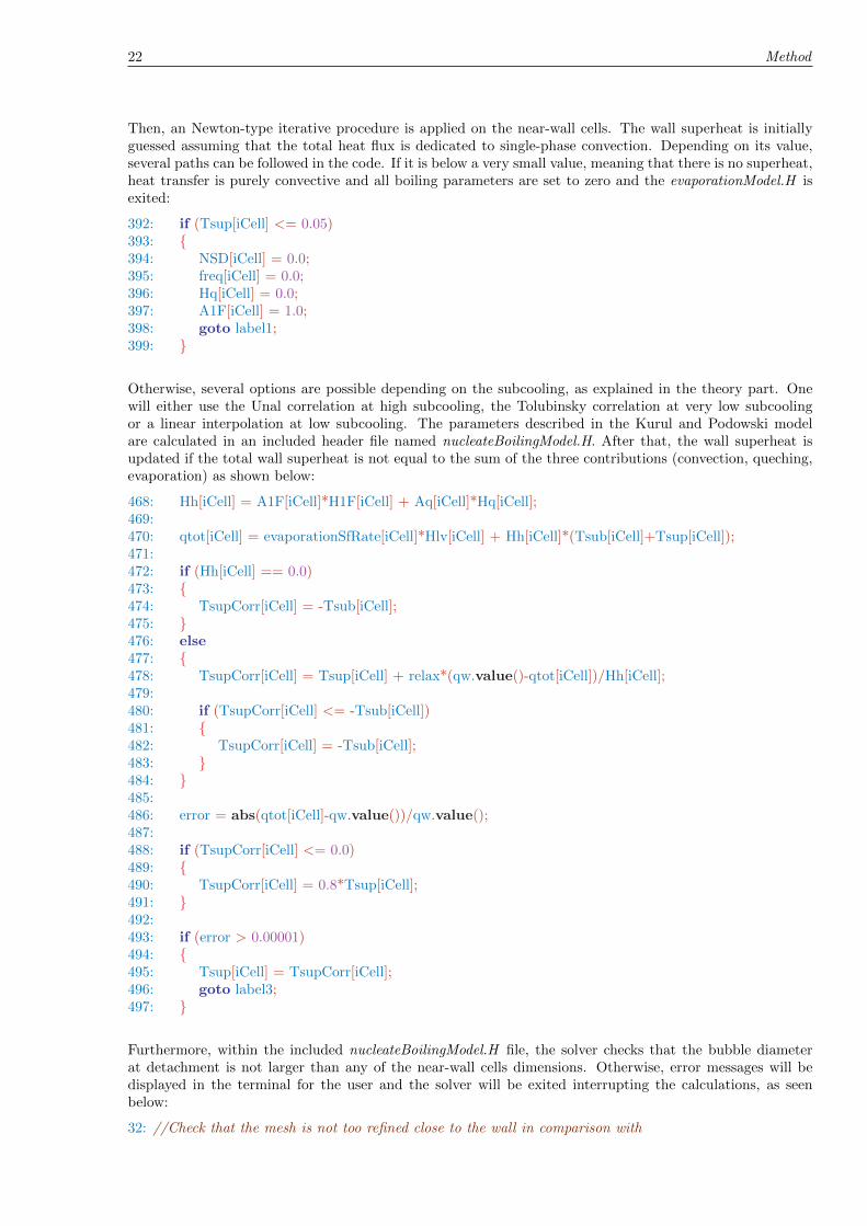
Then, an Newton-type iterative procedure is applied on the near-wall cells. The wall superheat is initiallyguessed assuming that the total heat flux is dedicated to single-phase convection. Depending on its value,several paths can be followed in the code. If it is below a very small value, meaning that there is no superheat,heat transfer is purely convective and all boiling parameters are set to zero and the evaporationModel.H isexited:
392: if (Tsup[iCell] <= 0.05)393: {394: NSD[iCell] = 0.0;395: freq[iCell] = 0.0;396: Hq[iCell] = 0.0;397: A1F[iCell] = 1.0;398: goto label1;399: }
Otherwise, several options are possible depending on the subcooling, as explained in the theory part. Onewill either use the Unal correlation at high subcooling, the Tolubinsky correlation at very low subcoolingor a linear interpolation at low subcooling. The parameters described in the Kurul and Podowski modelare calculated in an included header file named nucleateBoilingModel.H. After that, the wall superheat isupdated if the total wall superheat is not equal to the sum of the three contributions (convection, queching,evaporation) as shown below:
468: Hh[iCell] = A1F[iCell]*H1F[iCell] + Aq[iCell]*Hq[iCell];469:470: qtot[iCell] = evaporationSfRate[iCell]*Hlv[iCell] + Hh[iCell]*(Tsub[iCell]+Tsup[iCell]);471:472: if (Hh[iCell] == 0.0)473: {474: TsupCorr[iCell] = -Tsub[iCell];475: }476: else477: {478: TsupCorr[iCell] = Tsup[iCell] + relax*(qw.value()-qtot[iCell])/Hh[iCell];479:480: if (TsupCorr[iCell] <= -Tsub[iCell])481: {482: TsupCorr[iCell] = -Tsub[iCell];483: }484: }485:486: error = abs(qtot[iCell]-qw.value())/qw.value();487:488: if (TsupCorr[iCell] <= 0.0)489: {490: TsupCorr[iCell] = 0.8*Tsup[iCell];491: }492:493: if (error > 0.00001)494: {495: Tsup[iCell] = TsupCorr[iCell];496: goto label3;497: }
Furthermore, within the included nucleateBoilingModel.H file, the solver checks that the bubble diameterat detachment is not larger than any of the near-wall cells dimensions. Otherwise, error messages will bedisplayed in the terminal for the user and the solver will be exited interrupting the calculations, as seenbelow:
32: //Check that the mesh is not too refined close to the wall in comparison with

The solvers code explained 23
33: //bubbles size at departure34: if ( (dm.value()>xDim) || (dm.value()>yDim) || (dm.value()>zDim) )35: {36: Info<< ”ERROR : The mesh is too refined in comparison with the bubble size at departure”<< nl<< endl;37: Info<< ”IMPOSSIBLE to put all the energy of the created bubble in the near-wall cell ”<< nl <<endl;38:39: return 1;40: }
3.2.3 alphaEqn.H
Once the phase change rates are known, one can solve conservation equations, starting with the continuityequation for the gas phase. For numerical reasons, the form implemented is slightly different from what isshown in Eq.2.1 but the equation remains the same. Here, the conservation equation was divided by the voidfraction and a mixture flux phic as well as a relative flux are present in the equation. The continuous phasefraction is last deduced from the dispersed one by substracting the former to one.
10: fvScalarMatrix alphaEqn11: (12: fvm::ddt(alpha)13: + fvm::div(phic, alpha, scheme)14: + fvm::div(-fvc::flux(-phir, beta, schemer), alpha, schemer)15: ==16: (GammaGL-GammaLG)/rhoa17: );18:19: alphaEqn.relax();20: alphaEqn.solve();21:22: alpha = max(1.0e-8,alpha);23:24: beta = scalar(1) - alpha;
This loop can be repeated a predefined number of correction iterations, set in the fvSolution directory of thecase by the user.
3.2.4 IACEqn.H
The next step treats the interfacial area concentration (IAC) transport equation, which is essential in orderto determine the bubble diameter and the resulting interfacial forces. It begins with retrieving the sourcesterms by coalescence and breakup, respectively coalescenceSource and breakupSource, within the includedheader file breakupAndCoalescence.H. Then a field is created with a minimum value for the IAC to bound itto positive values:
01: # include ”breakupAndCoalescence.H”02:03: surfaceScalarField phiMix = phi;04: surfaceScalarField phiRel = phia - phib;05:06: dimensionedScalar smallIAC07: (08: ”smallIAC”,09: dimensionSet(0, -1, 0, 0, 0, 0, 0),10: scalar (1.0)11: );
24 Method
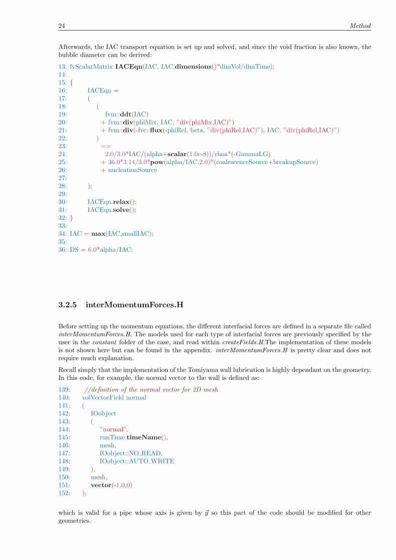
Afterwards, the IAC transport equation is set up and solved, and since the void fraction is also known, thebubble diameter can be derived:
13: fvScalarMatrix IACEqn(IAC, IAC.dimensions()*dimVol/dimTime);14:15: {16: IACEqn =17: (18: (19: fvm::ddt(IAC)20: + fvm::div(phiMix, IAC, ”div(phiMix,IAC)”)21: + fvm::div(-fvc::flux(-phiRel, beta, ”div(phiRel,IAC)”), IAC, ”div(phiRel,IAC)”)22: )23: ==24: 2.0/3.0*IAC/(alpha+scalar(1.0e-8))/rhoa*(-GammaLG)25: + 36.0*3.14/3.0*pow(alpha/IAC,2.0)*(coalescenceSource+breakupSource)26: + nucleationSource27:28: );29:30: IACEqn.relax();31: IACEqn.solve();32: }33:34: IAC = max(IAC,smallIAC);35:36: DS = 6.0*alpha/IAC;
3.2.5 interMomentumForces.H
Before setting up the momentum equations, the different interfacial forces are defined in a separate file calledinterMomentumForces.H. The models used for each type of interfacial forces are previously specified by theuser in the constant folder of the case, and read within createFields.H.The implementation of these modelsis not shown here but can be found in the appendix. interMomentumForces.H is pretty clear and does notrequire much explanation.
Recall simply that the implementation of the Tomiyama wall lubrication is highly dependant on the geometry.In this code, for example, the normal vector to the wall is defined as:
139: //definition of the normal vector for 2D mesh140: volVectorField normal141: (142: IOobject143: (144: ”normal”,145: runTime.timeName(),146: mesh,147: IOobject::NO READ,148: IOobject::AUTO WRITE149: ),150: mesh,151: vector(-1,0,0)152: );
which is valid for a pipe whose axis is given by ~y so this part of the code should be modified for othergeometries.
The solvers code explained 25
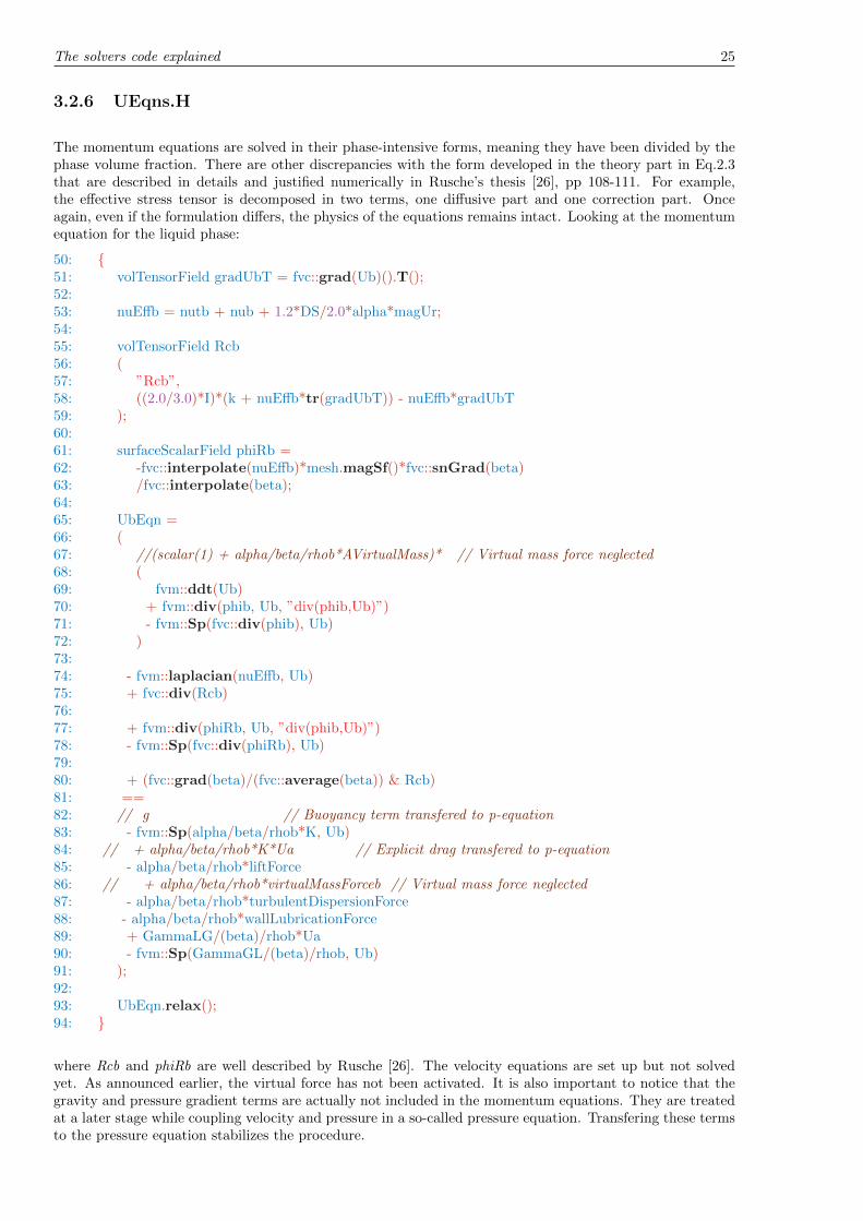
3.2.6 UEqns.H
The momentum equations are solved in their phase-intensive forms, meaning they have been divided by thephase volume fraction. There are other discrepancies with the form developed in the theory part in Eq.2.3that are described in details and justified numerically in Rusche’s thesis [26], pp 108-111. For example,the effective stress tensor is decomposed in two terms, one diffusive part and one correction part. Onceagain, even if the formulation differs, the physics of the equations remains intact. Looking at the momentumequation for the liquid phase:
50: {51: volTensorField gradUbT = fvc::grad(Ub)().T();52:53: nuEffb = nutb + nub + 1.2*DS/2.0*alpha*magUr;54:55: volTensorField Rcb56: (57: ”Rcb”,58: ((2.0/3.0)*I)*(k + nuEffb*tr(gradUbT)) - nuEffb*gradUbT59: );60:61: surfaceScalarField phiRb =62: -fvc::interpolate(nuEffb)*mesh.magSf()*fvc::snGrad(beta)63: /fvc::interpolate(beta);64:65: UbEqn =66: (67: //(scalar(1) + alpha/beta/rhob*AVirtualMass)* // Virtual mass force neglected68: (69: fvm::ddt(Ub)70: + fvm::div(phib, Ub, ”div(phib,Ub)”)71: - fvm::Sp(fvc::div(phib), Ub)72: )73:74: - fvm::laplacian(nuEffb, Ub)75: + fvc::div(Rcb)76:77: + fvm::div(phiRb, Ub, ”div(phib,Ub)”)78: - fvm::Sp(fvc::div(phiRb), Ub)79:80: + (fvc::grad(beta)/(fvc::average(beta)) & Rcb)81: ==82: // g // Buoyancy term transfered to p-equation83: - fvm::Sp(alpha/beta/rhob*K, Ub)84: // + alpha/beta/rhob*K*Ua // Explicit drag transfered to p-equation85: - alpha/beta/rhob*liftForce86: // + alpha/beta/rhob*virtualMassForceb // Virtual mass force neglected87: - alpha/beta/rhob*turbulentDispersionForce88: - alpha/beta/rhob*wallLubricationForce89: + GammaLG/(beta)/rhob*Ua90: - fvm::Sp(GammaGL/(beta)/rhob, Ub)91: );92:93: UbEqn.relax();94: }
where Rcb and phiRb are well described by Rusche [26]. The velocity equations are set up but not solvedyet. As announced earlier, the virtual force has not been activated. It is also important to notice that thegravity and pressure gradient terms are actually not included in the momentum equations. They are treatedat a later stage while coupling velocity and pressure in a so-called pressure equation. Transfering these termsto the pressure equation stabilizes the procedure.
26 Method
3.2.7 pEqn.H
As explained before, the velocity equations are set up but the velocity fields not calculated yet when the codeenters the pressure equation. The first step consists of predicting velocity fields from the matrices defined inUEqns.H. These predictions are not very accurate yet since they do not take pressure gradient nor gravityinto account. This is achieved in the following lines:
02: surfaceScalarField alphaf = fvc::interpolate(alpha);03: surfaceScalarField betaf = scalar(1) - alphaf;04:05: volScalarField rUaA = 1.0/UaEqn.A();06: volScalarField rUbA = 1.0/UbEqn.A();07:08: phia == (fvc::interpolate(Ua) & mesh.Sf());09: phib == (fvc::interpolate(Ub) & mesh.Sf());10:11: surfaceScalarField rUaAf = fvc::interpolate(rUaA);12: surfaceScalarField rUbAf = fvc::interpolate(rUbA);13:14: Ua = rUaA*UaEqn.H();15: Ub = rUbA*UbEqn.H();
Lines 5 and 6 retrieve and invert the central coefficients of the matrices defining the momentum equations.Multiplying these terms by the operation source from the same matrices in lines 14 and 15 yields to approx-imated velocity fields.
Interpolating these velocities at the cell face would yield to approximate fluxes. Then, corrections are appliedto the mass fluxes:
38: phia = (fvc::interpolate(Ua) & mesh.Sf()) + fvc::ddtPhiCorr(rUaA, Ua, phia)39: + phiDraga;40:41: phib = (fvc::interpolate(Ub) & mesh.Sf()) + fvc::ddtPhiCorr(rUbA, Ub, phib)42: + phiDragb;43:44: phi = alphaf*phia + betaf*phib;
where fvc::ddtPhiCorr introduces a correction due to the difference between the flux due to the interpolatedvelocities at the cell face and the real flux due to velocity, while phiDraga and phiDragb bring correctionsresulting from gravity. The latter are defined as:
38: phia = (fvc::interpolate(Ua) & mesh.Sf()) + fvc::ddtPhiCorr(rUaA, Ua, phia)39: + phiDraga;40:41: phib = (fvc::interpolate(Ub) & mesh.Sf()) + fvc::ddtPhiCorr(rUbA, Ub, phib)42: + phiDragb;43:44: phi = alphaf*phia + betaf*phib;
Then, the pressure equation is set-up and solved. This equation corresponds to a recasted version of thecontinuity equation expressed at cell faces, as explained by Rusche [26], pp. 112-113. This is done within afor-loop and several iterations may be necessary, if the mesh is non-orthogonal. Finally, the flux is completedby adding the pressure term. The obtained flux contains all physical contributions that occur in reality.Then, the phase fluxes are updated, as well as the velocities.
46: surfaceScalarField Dp(”(rho*(1|A(U)))”, alphaf*rUaAf/rhoa + betaf*rUbAf/rhob);47:48: for(int nonOrth=0; nonOrth<=nNonOrthCorr; nonOrth++)49: {50: fvScalarMatrix pEqn51: (

The solvers code explained 27
52: fvm::laplacian(Dp, p) == fvc::div(phi)53: );54:55: pEqn.setReference(pRefCell, pRefValue);56: pEqn.solve();57:58: if (nonOrth == nNonOrthCorr)59: {60: surfaceScalarField SfGradp = pEqn.flux()/Dp;61:62: phia -= rUaAf*SfGradp/rhoa;63: phib -= rUbAf*SfGradp/rhob;64: phi = alphaf*phia + betaf*phib;65:66: p.relax();67: SfGradp = pEqn.flux()/Dp;68:69: Ua += fvc::reconstruct(phiDraga - rUaAf*SfGradp/rhoa);70: Ua.correctBoundaryConditions();71:72: Ub += fvc::reconstruct(phiDragb - rUbAf*SfGradp/rhob);73: Ub.correctBoundaryConditions();74:75: U = alpha*Ua + beta*Ub;76: }77: }
3.2.8 HEqn.H
At this stage, the energy equation can be implemented according to Eq.2.5 in analogy with the liquid velocityequation. Once again, a phase intensive formulation has been chosen.
04: {05: volVectorField gradHb = fvc::grad(Hb);06:07: volScalarField AlphaEffb = nutb/PrandtlbT + lambdab/(rhob*Cpb);08:09: volVectorField Qcb10: (11: ”Qcb”,12: - AlphaEffb*gradHb13: );14:15: HbEqn =16: (17: (18: fvm::ddt(Hb)19: + fvm::div(phib, Hb, ”div(phib,Hb)”)20: - fvm::Sp(fvc::div(phib), Hb)21: )22:23: - fvm::laplacian(AlphaEffb, Hb)24: + (fvc::grad(beta)/(fvc::average(beta)) & Qcb)25:26: ==27:28: DpDt/rhob29: + GammaLG/(scalar(1.0)-alpha)/rhob*(Ha)30: - fvm::Sp(GammaGL/(beta)/rhob, Hb)
28 Method
31: + qw*SfPerVol/beta/rhob32: );33:34: HbEqn.relax();35: HbEqn.solve();36: }
where AlphaEffb and Qcb denote respectively the effective thermal diffusivity and the effective heat transferwithin the liquid phase. Lines 60 to 63 are the material derivative of the enthalpy. The first term on the RHSof the enthalpy equation is the energy gain by condensation, the second term is the energy loss by evaporationand the last one is the heat received from the heated wall. Recall that thanks to the field SfPerVol, this lastterm is non-zero only for near-wall cells.
3.2.9 kEpsilon.H
Lastly, the turbulent parameters are calculated as explained in the theory part. A classical k − ε model incombination with wall functions are used for the turbulence of the liquid phase if the turbulence is switched onby the user in the turbulenceProperties of the case. It starts with accumulating the wall contributions to theturbulent energy dissipation ε and to the buoyant production term G in the included header wallFunctions.H.Then the ε-equation is set. Before solving it, the terms of the ε-equation matrix that correspond to near-wallcells are removed because, as explained in the theory part, the ε-equation is not used in this region. This isperformed within wallDissipation.H. After this step, the ε-equation is solved.
12: #include ”wallFunctions.H”13:14: // Dissipation equation15: fvScalarMatrix epsEqn16: (17: fvm::ddt(beta, epsilon)18: + fvm::div(phib, epsilon)19: - fvm::laplacian20: (21: alphaEps*nuEffb, epsilon,22: ”laplacian(DepsilonEff,epsilon)”23: )24: ==25: C1*beta*G*epsilon/k26: - fvm::Sp(C2*beta*epsilon/k, epsilon)27: );28:29: #include ”wallDissipation.H”30:31: epsEqn.relax();32: epsEqn.solve();
Next, the k-equation is set and solved. Further on, the turbulent viscosity is calculating either directly or inwallViscosity.H for the near-wall cells.
37: // Turbulent kinetic energy equation38: fvScalarMatrix kEqn39: (40: fvm::ddt(beta, k)41: + fvm::div(phib, k)42: - fvm::laplacian43: (44: alphak*nuEffb, k,45: ”laplacian(DkEff,k)”46: )47: ==

Test cases 29
48: beta*G49: - fvm::Sp(beta*epsilon/k, k)50: );51: kEqn.relax();52: kEqn.solve();53:54: k.max(dimensionedScalar(”zero”, k.dimensions(), 1.0e-8));55:56: //- Re-calculate turbulence viscosity57: nutb = Cmu*sqr(k)/epsilon ;58:59: #include ”wallViscosity.H”
At the end, the effective viscosities of both phases are also updated.
62: nuEffb = nutb + nub + 1.2*DS/2.0*alpha*magUr;63: nuEffa = rhob/rhoa*nuEffb;
3.3 Test cases
3.3.1 The DEDALE experiment
The DEDALE experiment was carried out at EDF in 1995. One of its aims was to build up an importantdatabase for the validation of the NEPTUNE code, especially regarding the models used for interfacial forces,coalescence and breakup source terms and turbulence. It consists of an adiabatic vertical pipe of upwardsbubbly flows with an air/water system at atmospheric pressure (at the outlet) and a temperature of 30◦C(at the inlet). The transport properties of air and water under these conditions are shown in Table 3.1. Themethacrylate pipe is 6 m long and has an inner diameter of 0.0381 m. Air is injected at the periphery of thewater flow in 80 identical holes with an inner diameter of 0.6 mm.
Table 3.1: Transport properties of water and air in the DEDALE experiment
Property Value
p 1.0 barρl 995.65 kg/m3
ρg 1.165 kg/m3
λl 0.616 W/m/Kλg 0.026 W/m/Kcpl 4179.8 J/kg/Kcpg 1006.5 J/kg/Kνl 8.00·10−7 m2/sνg 1.60·10−5 m2/sσ 0.071 N/m
Measurements are realised at three different axial locations: y/D = 8, 55 and 155. At y/D = 8, the flowconditions are assumed to be the inlet ones. Void fraction, interfacial area concentration, bubble size andmean axial velocity, as well as mean and root mean square values of the liquid axial velocity are measuredlocally along the diameter at the three axial locations. A thorough description of the measurement deviceswill not be done here but one can refer to Bestion and Peturaud [4].
Of course, several tests were simulated with various combinations of inlet mass flux of air and water andwe have kept two of them to validate our code. These tests are DEDALE1101 and DEDALE1103 and theparameters measured at the inlet are presented in Table 3.2.
In OpenFOAM, an equivalent 2D-channel has been modeled, instead of a real 3D-pipe, in order to limit thecomputational needs and the time of the simulations. For the same reasons and using the axial symmetry ofthe channel, only one half of the channel is considered. The mesh is homogeneous and composed respectivelyof 20 cells and 200 cells in the radial and axial directions, what sets the first cell node at a distance of

30 Method
Table 3.2: DEDALE1101 and DEDALE1103 measured inlet conditions
Property DEDALE1101 DEDALE1103
Liquid superficial velocity Jl 0.877 m/s 0.877 m/sGas superficial velocity Jg 0.0588 m/s 0.1851 m/s
α 0.048 0.152kl 4.23·10−3 m2/s2 1.78·10−2 m2/s2
ai 97 m−1 269 m−1
x+ ∼ 20. A view of the mesh and its radial decomposition is shown in Figure 3.4.
Figure 3.4: Zoom on the grid used for the DEDALE simulations
Initial and boundary conditions that have been applied are resumed in Table 3.3 and 3.4. The solverdeals with real phase velocities and not superficial phase velocities which are the parameters given from themeasurements. The former are thus calculated from the latter using a drift-flux model, whose distributionfactor has been fixed so that the void fraction derived from the drift-flux model fits the void fraction measuredat the inlet in the experiment. Another remark is that the boundary conditions at the inlet are taken uniform,what is of course not exact, since the inlet of the simulation refers in reality to the axial position y/D = 8where the flow is developed. This choice for the simulations origins from the lack of data regarding the radialprofile at y/D = 8 where only mean values are given. It must also be noted that the pressure p is set to 0.The real value of the pressure is used through an additional field pReal read from the transportPropertiesfile, and it is added to the calculated pressure field p, which indeed only refers to the deviation from thereference value pReal.
Table 3.3: Initial and boundary conditions applied in OpenFOAM for DEDALE1101
Field Initial Inlet Outlet Wall Centerline
Ul [m/s] 0.916 0.916 zeroGradient 0 symmetryPlaneUg [m/s] 1.365 1.365 zeroGradient 0 symmetryPlane
α 0.048 0.048 zeroGradient zeroGradient symmetryPlanep 0 zeroGradient 0 zeroGradient symmetryPlane
ai [m−1] 97 97 zeroGradient zeroGradient symmetryPlanek [m2/s2] 4.23·10−3 4.23·10−3 zeroGradient zeroGradient symmetryPlaneε [m2/s3] 1.695·10−2 1.695·10−2 zeroGradient zeroGradient symmetryPlane
3.3.2 The DEBORA experiment
The DEBORA experiment was carried out in 2000 by the CEA. This experiment differs from DEDALE sinceit aims to analyse upwards bubbly two-phase flows with phase change (both nucleation at the wall andcondensation in the bulk). Its main goal was to provide a large data set covering for boiling in PWR up toDNB. However, it is both complex and costly to set up experimental facility at high pressure. Therefore,the choice has been made to use R12 which behaves at low pressure in a same manner as water under PWRconditions. The liquid-vapor density ratio in these experiments corresponds to that of water-steam at 95-150bar.

Test cases 31
Table 3.4: Initial and boundary conditions applied in OpenFOAM for DEDALE1103
Field Initial Inlet Outlet Wall Centerline
Ul [m/s] 1.0157 1.0157 zeroGradient 0 symmetryPlaneUg [m/s] 1.355 1.355 zeroGradient 0 symmetryPlane
α 0.152 0.152 zeroGradient zeroGradient symmetryPlanep 0 zeroGradient 0 zeroGradient symmetryPlane
ai [m−1] 269 269 zeroGradient zeroGradient symmetryPlanek [m2/s2] 1.78·10−2 1.78·10−2 zeroGradient zeroGradient symmetryPlaneε [m2/s3] 1.695·10−2 1.695·10−2 zeroGradient zeroGradient symmetryPlane
DEBORA consists of a vertical pipe made of Inconel 600, whose physical properties can be seen in Table3.5, with an inner diameter equal to 19.2 mm. Axially, it is divided into three parts: the adiabatic inletsection (1 m length), the heated section (3.5 m length) and the adiabatic outlet section (0.5 m). Theintermediate section is heated with an electric heating system imposing a unifrom or non-uniform heat fluxdensity. Subcooled R12 is fed at the bottom of the pipe, vapor bubbles are formed at the heated wall andmigrate to the bulk where they condensate.
Table 3.5: Properties of Inconel 600 used as pipe material in the DEBORA experiment
Property Value
ρw 8430 kg/m3
λw 15.0 W/m/Kcpw 444 J/kg/K
The measurements of radial distributions are performed at one axial location only, at the end of the heatedsection, but for 20 different radial positions. The radial profiles of void fraction and bubble diameters aremeasured by means of an optical probe. Besides, the liquid temperature radial profile is obtained by meansof thermocouples.
Here as well, various experiments have been performed, combining different input parameters. The caseswhich are used for the validation of the present solver were all uniformly heated, and their experimentalconditions are presented in Table 3.6 and the transport properties of R12 under these conditions are shownin Table 3.7.
Table 3.6: DEBORA selected cases and their experimental conditions
Case Pressure Mass flow rate Wall heat flux density Inlet temperature[bar] [kg/m2/s] [kW/m2] [◦C]
DEB5 26.15 1986 73.89 68.52DEB6 26.15 1984.9 73.89 70.53DEB10 14.59 2027.8 76.24 34.91DEB13 26.17 2980.9 109.42 69.20
In OpenFOAM, the geometry created is again a simplified version: half of a 2D-pipe is created to modelthis experiment. Furthermore, one will only simulate the 3.5 m long heated part, neglecting the adiabaticinlet section. Once again, the grid is homogeneous with 20 cells in the radial direction and 250 cells in theaxial direction, as it has been done by Lopez De Bertodano and Prabhudharwadkar [23]. Near-wall cells arethus located at a distance x+ ∼ 60. Finally, the initial and boundary conditions used in OpenFOAM aresummarised in Table 3.8, 3.9, 3.10 and 3.11. The same comment on the field p can be made: it representsindeed the deviation from a reference pressure. It must be observed that the initial and inlet values takenfor Ug and ai, while α is null, will not affect the final results after convergence of the code, but it might benecessary to chose them rather close to their final values for stability’s sake.

32 Method
Table 3.7: Transport properties of R12 in the selected DEBORA cases
Property DEB5,DEB6 DEB10 DEB13
ρl [kg/m3] 1017.1 1177.2 1016.8ρg [kg/m3] 172.06 84.91 172.24λl [W/m/K] 4.57·10−2 5.58·10−2 4.57·10−2
λg [W/m/K] 1.76·10−2 4.65·10−2 1.76·10−2
cpl [J/kg/K] 1419.8 1111.50 1420.7cpg [J/kg/K] 1290.8 861.71 1292.0νl [m2/s] 8.80·10−8 1.12·10−7 8.80·10−8
νg [m2/s] 9.13·10−8 1.55·10−7 9.13·10−8
σ [N/m] 1.77·10−3 4.65·10−3 1.77·10−3
Tsat [◦C] 86.64 58.15 86.64il,sat [J/kg/K] 292530.0 258450.0 292590.0ilg [J/kg/K] 86070.0 116100.0 86010.0
Table 3.8: Initial and boundary conditions used in OpenFOAM for DEB5
Field Initial Inlet Outlet Wall Centerline
Ul [m/s] 1.744 1.744 zeroGradient 0 symmetryPlaneUg [m/s] 1.9 1.9 zeroGradient 0 symmetryPlane
α 0 0 zeroGradient zeroGradient symmetryPlanep 0 zeroGradient 0 zeroGradient symmetryPlane
ai [m−1] 5000 5000 zeroGradient zeroGradient symmetryPlanek [m2/s2] 1.14·10−2 1.14·10−2 zeroGradient zeroGradient symmetryPlaneε [m2/s3] 1.49·10−1 1.49·10−1 zeroGradient zeroGradient symmetryPlaneil [J/kg] 269740.0 269740.0 zeroGradient zeroGradient symmetryPlane
Table 3.9: Initial and boundary conditions used in OpenFOAM for DEB6
Field Initial Inlet Outlet Wall Centerline
Ul [m/s] 1.76 1.76 zeroGradient 0 symmetryPlaneUg [m/s] 1.9 1.9 zeroGradient 0 symmetryPlane
α 0 0 zeroGradient zeroGradient symmetryPlanep 0 zeroGradient 0 zeroGradient symmetryPlane
ai [m−1] 2000 2000 zeroGradient zeroGradient symmetryPlanek [m2/s2] 1.16·10−2 1.16·10−2 zeroGradient zeroGradient symmetryPlaneε [m2/s3] 1.53·10−1 1.53·10−1 zeroGradient zeroGradient symmetryPlaneil [J/kg] 272060.0 272060.0 zeroGradient zeroGradient symmetryPlane
Table 3.10: Initial and boundary conditions used in OpenFOAM for DEB10
Field Initial Inlet Outlet Wall Centerline
Ul [m/s] 1.586 1.586 zeroGradient 0 symmetryPlaneUg [m/s] 1.8 1.8 zeroGradient 0 symmetryPlane
α 0 0 zeroGradient zeroGradient symmetryPlanep 0 zeroGradient 0 zeroGradient symmetryPlane
ai [m−1] 2000 2000 zeroGradient zeroGradient symmetryPlanek [m2/s2] 9.43·10−3 9.43·10−3 zeroGradient zeroGradient symmetryPlaneε [m2/s3] 1.12·10−1 1.12·10−1 zeroGradient zeroGradient symmetryPlaneil [J/kg] 234030.0 234030.0 zeroGradient zeroGradient symmetryPlane

Test cases 33
Table 3.11: Initial and boundary conditions used in OpenFOAM for DEB13
Field Initial Inlet Outlet Wall Centerline
Ul [m/s] 2.626 2.626 zeroGradient 0 symmetryPlaneUg [m/s] 2.9 2.9 zeroGradient 0 symmetryPlane
α 0 0 zeroGradient zeroGradient symmetryPlanep 0 zeroGradient 0 zeroGradient symmetryPlane
ai [m−1] 2000 2000 zeroGradient zeroGradient symmetryPlanek [m2/s2] 2.59·10−2 2.59·10−2 zeroGradient zeroGradient symmetryPlaneε [m2/s3] 5.08·10−1 5.08·10−1 zeroGradient zeroGradient symmetryPlaneil [J/kg] 270520.0 270520.0 zeroGradient zeroGradient symmetryPlane
34 Method
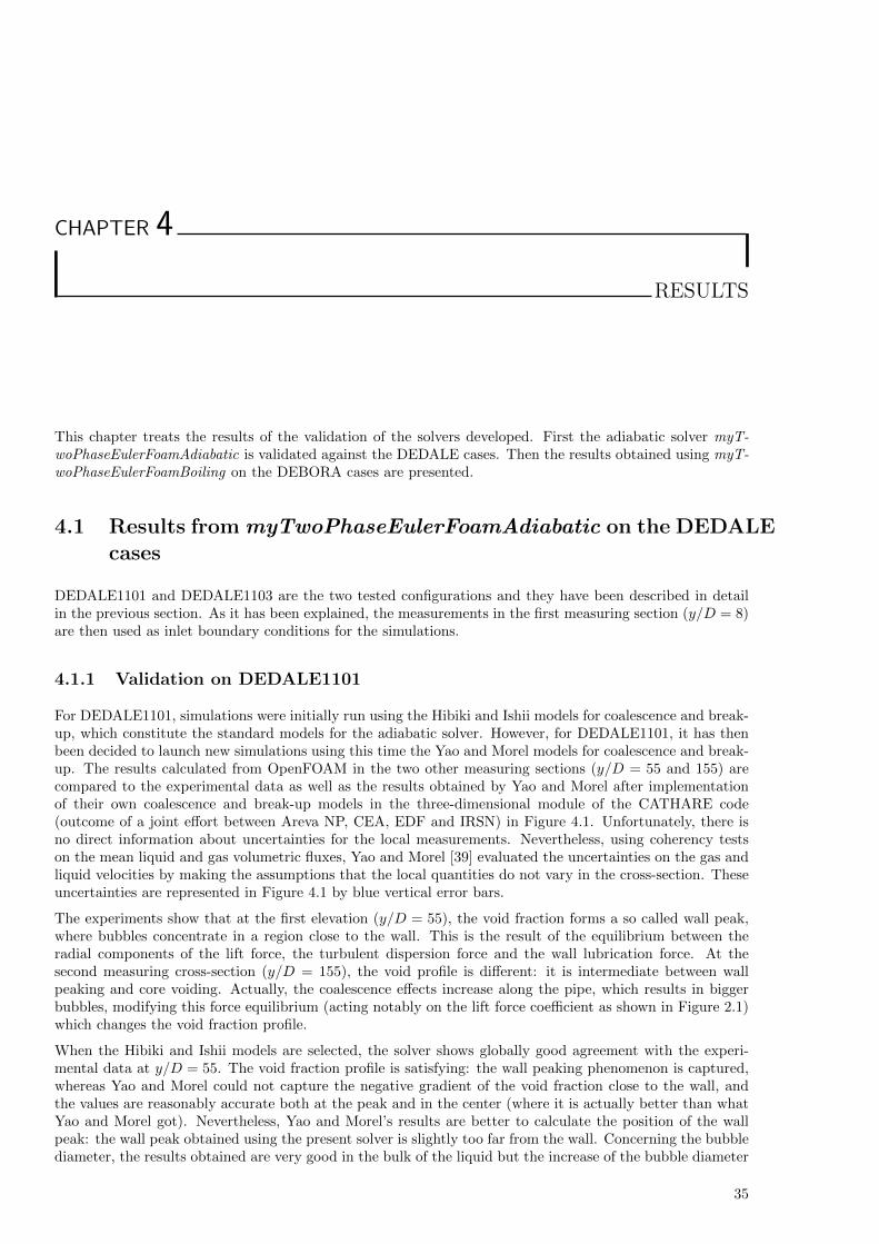
CHAPTER 4
RESULTS
This chapter treats the results of the validation of the solvers developed. First the adiabatic solver myT-woPhaseEulerFoamAdiabatic is validated against the DEDALE cases. Then the results obtained using myT-woPhaseEulerFoamBoiling on the DEBORA cases are presented.
4.1 Results from myTwoPhaseEulerFoamAdiabatic on the DEDALEcases
DEDALE1101 and DEDALE1103 are the two tested configurations and they have been described in detailin the previous section. As it has been explained, the measurements in the first measuring section (y/D = 8)are then used as inlet boundary conditions for the simulations.
4.1.1 Validation on DEDALE1101
For DEDALE1101, simulations were initially run using the Hibiki and Ishii models for coalescence and break-up, which constitute the standard models for the adiabatic solver. However, for DEDALE1101, it has thenbeen decided to launch new simulations using this time the Yao and Morel models for coalescence and break-up. The results calculated from OpenFOAM in the two other measuring sections (y/D = 55 and 155) arecompared to the experimental data as well as the results obtained by Yao and Morel after implementationof their own coalescence and break-up models in the three-dimensional module of the CATHARE code(outcome of a joint effort between Areva NP, CEA, EDF and IRSN) in Figure 4.1. Unfortunately, there isno direct information about uncertainties for the local measurements. Nevertheless, using coherency testson the mean liquid and gas volumetric fluxes, Yao and Morel [39] evaluated the uncertainties on the gas andliquid velocities by making the assumptions that the local quantities do not vary in the cross-section. Theseuncertainties are represented in Figure 4.1 by blue vertical error bars.
The experiments show that at the first elevation (y/D = 55), the void fraction forms a so called wall peak,where bubbles concentrate in a region close to the wall. This is the result of the equilibrium between theradial components of the lift force, the turbulent dispersion force and the wall lubrication force. At thesecond measuring cross-section (y/D = 155), the void profile is different: it is intermediate between wallpeaking and core voiding. Actually, the coalescence effects increase along the pipe, which results in biggerbubbles, modifying this force equilibrium (acting notably on the lift force coefficient as shown in Figure 2.1)which changes the void fraction profile.
When the Hibiki and Ishii models are selected, the solver shows globally good agreement with the experi-mental data at y/D = 55. The void fraction profile is satisfying: the wall peaking phenomenon is captured,whereas Yao and Morel could not capture the negative gradient of the void fraction close to the wall, andthe values are reasonably accurate both at the peak and in the center (where it is actually better than whatYao and Morel got). Nevertheless, Yao and Morel’s results are better to calculate the position of the wallpeak: the wall peak obtained using the present solver is slightly too far from the wall. Concerning the bubblediameter, the results obtained are very good in the bulk of the liquid but the increase of the bubble diameter
35
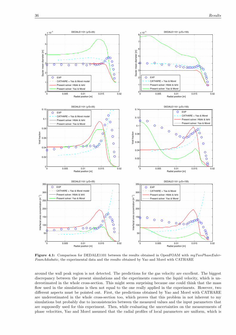
36 Results
0 0.005 0.01 0.015 0.020
1
2
3
4
5
6x 10
−3
Saute
r m
ean d
iam
ete
r [m
]
DEDALE1101 (y/D=55)
Radial position [m]
EXP
CATHARE + Yao & Morel model
Present solver: Hibiki & Ishii
Present solver: Yao & Morel
0 0.005 0.01 0.015 0.020
1
2
3
4
5
6
7
8x 10
−3
Saute
r m
ean d
iam
ete
r [m
]
DEDALE1101 (y/D=155)
Radial position [m]
EXP
CATHARE + Yao & Morel
Present solver: Hibiki & Ishii
Present solver: Yao & Morel
0 0.005 0.01 0.015 0.020
0.02
0.04
0.06
0.08
0.1
0.12
Void
fra
ction
DEDALE1101 (y/D=55)
Radial position [m]
EXP
CATHARE + Yao & Morel model
Present solver: Hibiki & Ishii
Present solver: Yao & Morel
0 0.005 0.01 0.015 0.020
0.02
0.04
0.06
0.08
0.1
0.12
0.14
Void
fra
ction
DEDALE1101 (y/D=155)
Radial position [m]
EXP
CATHARE + Yao & Morel
Present solver: Hibiki & Ishii
Present solver: Yao & Morel
0 0.005 0.01 0.015 0.020
50
100
150
200
250
300
350
Inte
rfacia
l are
a c
oncentr
ation [m
−1]
DEDALE1101 (y/D=55)
Radial position [m]
EXP
CATHARE + Yao & Morel model
Present solver: Hibiki & Ishii
Present solver: Yao & Morel
0 0.005 0.01 0.015 0.020
50
100
150
200
250
300
350
Inte
rfacia
l are
a c
oncentr
ation [m
−1]
DEDALE1101 (y/D=155)
Radial position [m]
EXP
CATHARE + Yao & Morel
Present solver: Hibiki & Ishii
Present solver: Yao & Morel
Figure 4.1: Comparison for DEDALE1101 between the results obtained in OpenFOAM with myTwoPhaseEuler-FoamAdiabatic, the experimental data and the results obtained by Yao and Morel with CATHARE
around the wall peak region is not detected. The predictions for the gas velocity are excellent. The biggestdiscrepancy between the present simulations and the experiments concern the liquid velocity, which is un-derestimated in the whole cross-section. This might seem surprising because one could think that the massflow used in the simulations is then not equal to the one really applied in the experiments. However, twodifferent aspects must be pointed out. First, the predictions obtained by Yao and Morel with CATHAREare underestimated in the whole cross-section too, which proves that this problem in not inherent to mysimulations but probably due to inconsistencies between the measured values and the input parameters thatare supposedly used for this experiment. Then, while evaluating the uncertainties on the measurements ofphase velocities, Yao and Morel assumed that the radial profiles of local parameters are uniform, which is
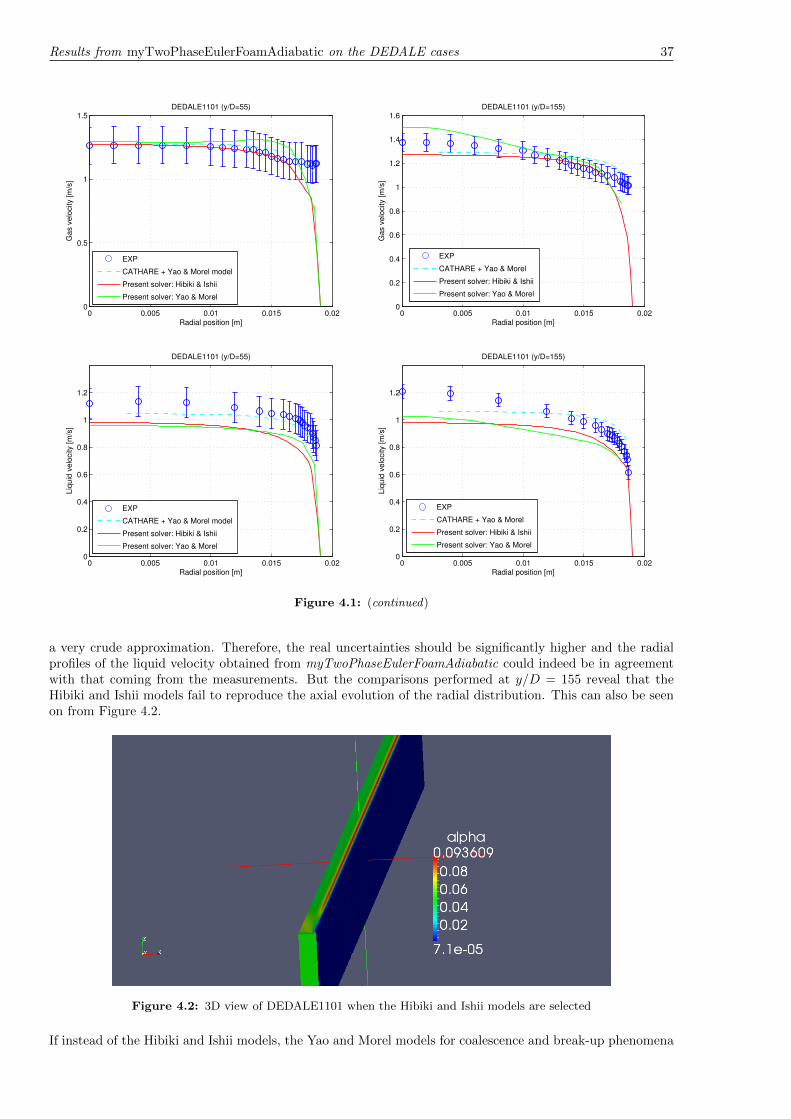
Results from myTwoPhaseEulerFoamAdiabatic on the DEDALE cases 37
0 0.005 0.01 0.015 0.020
0.5
1
1.5
Gas v
elo
city [m
/s]
DEDALE1101 (y/D=55)
Radial position [m]
EXP
CATHARE + Yao & Morel model
Present solver: Hibiki & Ishii
Present solver: Yao & Morel
0 0.005 0.01 0.015 0.020
0.2
0.4
0.6
0.8
1
1.2
1.4
1.6
Gas v
elo
city [m
/s]
DEDALE1101 (y/D=155)
Radial position [m]
EXP
CATHARE + Yao & Morel
Present solver: Hibiki & Ishii
Present solver: Yao & Morel
0 0.005 0.01 0.015 0.020
0.2
0.4
0.6
0.8
1
1.2
Liq
uid
velo
city [m
/s]
DEDALE1101 (y/D=55)
Radial position [m]
EXP
CATHARE + Yao & Morel model
Present solver: Hibiki & Ishii
Present solver: Yao & Morel
0 0.005 0.01 0.015 0.020
0.2
0.4
0.6
0.8
1
1.2
Liq
uid
velo
city [m
/s]
DEDALE1101 (y/D=155)
Radial position [m]
EXP
CATHARE + Yao & Morel
Present solver: Hibiki & Ishii
Present solver: Yao & Morel
Figure 4.1: (continued)
a very crude approximation. Therefore, the real uncertainties should be significantly higher and the radialprofiles of the liquid velocity obtained from myTwoPhaseEulerFoamAdiabatic could indeed be in agreementwith that coming from the measurements. But the comparisons performed at y/D = 155 reveal that theHibiki and Ishii models fail to reproduce the axial evolution of the radial distribution. This can also be seenon from Figure 4.2.
Figure 4.2: 3D view of DEDALE1101 when the Hibiki and Ishii models are selected
If instead of the Hibiki and Ishii models, the Yao and Morel models for coalescence and break-up phenomena
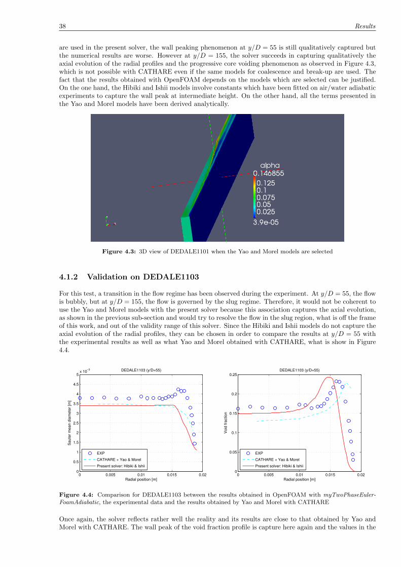
38 Results
are used in the present solver, the wall peaking phenomenon at y/D = 55 is still qualitatively captured butthe numerical results are worse. However at y/D = 155, the solver succeeds in capturing qualitatively theaxial evolution of the radial profiles and the progressive core voiding phenomenon as observed in Figure 4.3,which is not possible with CATHARE even if the same models for coalescence and break-up are used. Thefact that the results obtained with OpenFOAM depends on the models which are selected can be justified.On the one hand, the Hibiki and Ishii models involve constants which have been fitted on air/water adiabaticexperiments to capture the wall peak at intermediate height. On the other hand, all the terms presented inthe Yao and Morel models have been derived analytically.
Figure 4.3: 3D view of DEDALE1101 when the Yao and Morel models are selected
4.1.2 Validation on DEDALE1103
For this test, a transition in the flow regime has been observed during the experiment. At y/D = 55, the flowis bubbly, but at y/D = 155, the flow is governed by the slug regime. Therefore, it would not be coherent touse the Yao and Morel models with the present solver because this association captures the axial evolution,as shown in the previous sub-section and would try to resolve the flow in the slug region, what is off the frameof this work, and out of the validity range of this solver. Since the Hibiki and Ishii models do not capture theaxial evolution of the radial profiles, they can be chosen in order to compare the results at y/D = 55 withthe experimental results as well as what Yao and Morel obtained with CATHARE, what is show in Figure4.4.
0 0.005 0.01 0.015 0.020
0.5
1
1.5
2
2.5
3
3.5
4
4.5
5x 10
−3
Saute
r m
ean d
iam
ete
r [m
]
DEDALE1103 (y/D=55)
Radial position [m]
EXP
CATHARE + Yao & Morel
Present solver: Hibiki & Ishii
0 0.005 0.01 0.015 0.020
0.05
0.1
0.15
0.2
0.25
Void
fra
ction
DEDALE1103 (y/D=55)
Radial position [m]
EXP
CATHARE + Yao & Morel
Present solver: Hibiki & Ishii
Figure 4.4: Comparison for DEDALE1103 between the results obtained in OpenFOAM with myTwoPhaseEuler-FoamAdiabatic, the experimental data and the results obtained by Yao and Morel with CATHARE
Once again, the solver reflects rather well the reality and its results are close to that obtained by Yao andMorel with CATHARE. The wall peak of the void fraction profile is capture here again and the values in the
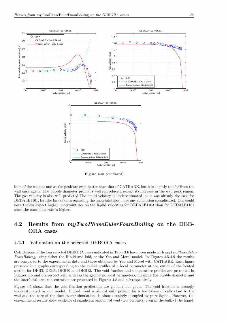
Results from myTwoPhaseEulerFoamBoiling on the DEBORA cases 39
0 0.005 0.01 0.015 0.020
100
200
300
400
500
600
700
Inte
rfacia
l are
a c
oncentr
ation [m
−1]
DEDALE1103 (y/D=55)
Radial position [m]
EXP
CATHARE + Yao & Morel
Present solver: Hibiki & Ishii
0 0.005 0.01 0.015 0.020
0.2
0.4
0.6
0.8
1
1.2
1.4
1.6
Gas v
elo
city [m
/s]
DEDALE1103 (y/D=55)
Radial position [m]
EXP
CATHARE + Yao & Morel
Present solver: Hibiki & Ishii
0 0.005 0.01 0.015 0.020
0.5
1
1.5
Liq
uid
velo
city [m
/s]
DEDALE1103 (y/D=55)
Radial position [m]
EXP
CATHARE + Yao & Morel
Present solver: Hibiki & Ishii
Figure 4.4: (continued)
bulk of the coolant and at the peak are even better than that of CATHARE, but it is slightly too far from thewall once again. The bubble diameter profile is well reproduced, except its increase in the wall peak region.The gas velocity is also well predicted.The liquid velocity is underestimated, as it was already the case forDEDALE1101, but the lack of data regarding the uncertaintities make any conclusion complicated. One couldnevertheless expect higher uncertaintities on the liquid velocities for DEDALE1103 than for DEDALE1101since the mass flow rate is higher.
4.2 Results from myTwoPhaseEulerFoamBoiling on the DEB-ORA cases
4.2.1 Validation on the selected DEBORA cases
Calculations of the four selected DEBORA cases indicated in Table 3.6 have been made with myTwoPhaseEuler-FoamBoiling, using either the Hibiki and Ishi, or the Yao and Morel model. In Figures 4.5-4.9 the resultsare compared to the experimental data and those obtained by Yao and Morel with CATHARE. Each figurepresents four graphs corresponding to the radial profiles of a local parameter at the outlet of the heatedsection for DEB5, DEB6, DEB10 and DEB13. The void fraction and temperature profiles are presented inFigures 4.5 and 4.7 respectively whereas the geometric local parameters, meaning the bubble diameter andthe interfacial area concentration are presented in Figures 4.8 and 4.9 respectively.
Figure 4.5 shows that the void fraction predictions are globally not good. The void fraction is stronglyunderestimated by our model. Indeed, void is almost only present for a few layers of cells close to thewall and the core of the duct in our simulations is almost entirely occupied by pure liquid. However, theexperimental results show evidence of significant amount of void (few percents) even in the bulk of the liquid.
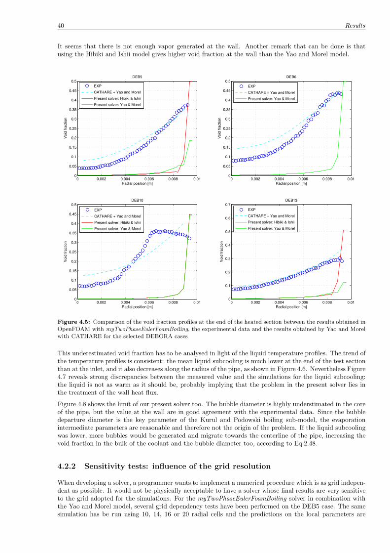
40 Results
It seems that there is not enough vapor generated at the wall. Another remark that can be done is thatusing the Hibiki and Ishii model gives higher void fraction at the wall than the Yao and Morel model.
0 0.002 0.004 0.006 0.008 0.010
0.05
0.1
0.15
0.2
0.25
0.3
0.35
0.4
0.45
0.5
Void
fra
ction
DEB5
Radial position [m]
EXP
CATHARE + Yao and Morel
Present solver: Hibiki & Ishii
Present solver: Yao & Morel
0 0.002 0.004 0.006 0.008 0.010
0.05
0.1
0.15
0.2
0.25
0.3
0.35
0.4
0.45
0.5
Void
fra
ction
DEB6
Radial position [m]
EXP
CATHARE + Yao and Morel
Present solver: Yao & Morel
0 0.002 0.004 0.006 0.008 0.010
0.05
0.1
0.15
0.2
0.25
0.3
0.35
0.4
0.45
0.5
Void
fra
ction
Radial position [m]
DEB10
EXP
CATHARE + Yao and Morel
Present solver: Hibiki & Ishii
Present solver: Yao & Morel
0 0.002 0.004 0.006 0.008 0.010
0.1
0.2
0.3
0.4
0.5
0.6
0.7
Void
fra
ction
Radial position [m]
DEB13
EXP
CATHARE + Yao and Morel
Present solver: Hibiki & Ishii
Present solver: Yao & Morel
Figure 4.5: Comparison of the void fraction profiles at the end of the heated section between the results obtained inOpenFOAM with myTwoPhaseEulerFoamBoiling, the experimental data and the results obtained by Yao and Morelwith CATHARE for the selected DEBORA cases
This underestimated void fraction has to be analysed in light of the liquid temperature profiles. The trend ofthe temperature profiles is consistent: the mean liquid subcooling is much lower at the end of the test sectionthan at the inlet, and it also decreases along the radius of the pipe, as shown in Figure 4.6. Nevertheless Figure4.7 reveals strong discrepancies between the measured value and the simulations for the liquid subcooling:the liquid is not as warm as it should be, probably implying that the problem in the present solver lies inthe treatment of the wall heat flux.
Figure 4.8 shows the limit of our present solver too. The bubble diameter is highly understimated in the coreof the pipe, but the value at the wall are in good agreement with the experimental data. Since the bubbledeparture diameter is the key parameter of the Kurul and Podowski boiling sub-model, the evaporationintermediate parameters are reasonable and therefore not the origin of the problem. If the liquid subcoolingwas lower, more bubbles would be generated and migrate towards the centerline of the pipe, increasing thevoid fraction in the bulk of the coolant and the bubble diameter too, according to Eq.2.48.
4.2.2 Sensitivity tests: influence of the grid resolution
When developing a solver, a programmer wants to implement a numerical procedure which is as grid indepen-dent as possible. It would not be physically acceptable to have a solver whose final results are very sensitiveto the grid adopted for the simulations. For the myTwoPhaseEulerFoamBoiling solver in combination withthe Yao and Morel model, several grid dependency tests have been performed on the DEB5 case. The samesimulation has be run using 10, 14, 16 or 20 radial cells and the predictions on the local parameters are
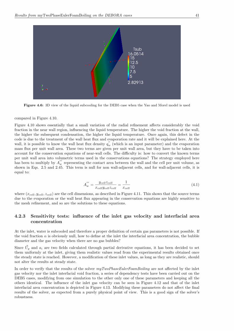
Results from myTwoPhaseEulerFoamBoiling on the DEBORA cases 41
Figure 4.6: 3D view of the liquid subcooling for the DEB5 case when the Yao and Morel model is used
compared in Figure 4.10.
Figure 4.10 shows essentially that a small variation of the radial refinement affects considerably the voidfraction in the near wall region, influencing the liquid temperature. The higher the void fraction at the wall,the higher the subsequent condensation, the higher the liquid temperature. Once again, this defect in thecode is due to the treatment of the wall heat flux and evaporation rate and it will be explained here. At thewall, it is possible to know the wall heat flux density q
′′
w (which is an input parameter) and the evaporationmass flux per unit wall area. These two terms are given per unit wall area, but they have to be taken intoaccount for the conservation equations of near-wall cells. The difficulty is: how to convert the known termsper unit wall area into volumetric terms used in the conservations equations? The strategy employed herehas been to multiply by A
′′′
w representing the contact area between the wall and the cell per unit volume, asshown in Eqs. 2.5 and 2.45. This term is null for non wall-adjacent cells, and for wall-adjacent cells, it isequal to:
A′′′
w =ycellzcell
xcellycellzcell=
1
xcell(4.1)
where (xcell, ycell, zcell) are the cell dimensions, as described in Figure 4.11. This shows that the source termsdue to the evaporation or the wall heat flux appearing in the conservation equations are highly sensitive tothe mesh refinement, and so are the solutions to these equations.
4.2.3 Sensitivity tests: influence of the inlet gas velocity and interfacial areaconcentration
At the inlet, water is subcooled and therefore a proper definition of certain gas parameters is not possible. Ifthe void fraction α is obviously null, how to define at the inlet the interfacial area concentration, the bubblediameter and the gas velocity when there are no gas bubbles?
Since ~Ug and ai are two fields calculated through partial derivative equations, it has been decided to setthem uniformly at the inlet, giving them realistic values read from the experimental results obtained oncethe steady state is reached. However, a modification of these inlet values, as long as they are realistic, shouldnot alter the results at steady state.
In order to verify that the results of the solver myTwoPhaseEulerFoamBoiling are not affected by the inletgas velocity nor the inlet interfacial void fraction, a series of dependency tests have been carried out on theDEB5 cases, modifying from one simulation to the other only one of these parameters and keeping all theothers identical. The influence of the inlet gas velocity can be seen in Figure 4.12 and that of the inletinterfacial area concentration is depicted in Figure 4.13. Modifying these parameters do not affect the finalresults of the solver, as expected from a purely physical point of view. This is a good sign of the solver’srobustness.

42 Results
0 0.002 0.004 0.006 0.008 0.0178
79
80
81
82
83
84
85
86
87
88
Liq
uid
tem
pera
ture
[°C
]
DEB5
Radial position [m]
EXP
CATHARE + Yao and Morel
Present solver: Hibiki & Ishii
Present solver: Yao & Morel
Tsat
0 0.002 0.004 0.006 0.008 0.0179
80
81
82
83
84
85
86
87
88
Liq
uid
tem
pera
ture
[°C
]
DEB6
Radial position [m]
EXP
CATHARE + Yao and Morel
Present solver: Yao & Morel
Tsat
0 0.002 0.004 0.006 0.008 0.0145
50
55
60
Liq
uid
tem
pera
ture
[°C
]
Radial position [m]
DEB10
CATHARE + Yao and Morel
Present solver: Hibiki & Ishii
Present solver: Yao & Morel
Tsat
0 0.002 0.004 0.006 0.008 0.0178
79
80
81
82
83
84
85
86
87
88
Liq
uid
tem
pera
ture
[°C
]
Radial position [m]
DEB13
CATHARE + Yao and Morel
Present solver: Hibiki & Ishii
Present solver: Yao & Morel
Tsat
Figure 4.7: Comparison of the liquid temperature profiles at the end of the heated section between the resultsobtained in OpenFOAM with myTwoPhaseEulerFoamBoiling, the experimental data and the results obtained by Yaoand Morel with CATHARE for the selected DEBORA cases

Results from myTwoPhaseEulerFoamBoiling on the DEBORA cases 43
0 0.002 0.004 0.006 0.008 0.010
1
2
3
4
5
6x 10
−4
Saute
r m
ean d
iam
ete
r [m
]
DEB5
Radial position [m]
EXP
CATHARE + Yao and Morel
Present solver: Hibiki & Ishii
Present solver: Yao & Morel
0 0.002 0.004 0.006 0.008 0.010
1
2
3
4
5
6x 10
−4
Saute
r m
ean d
iam
ete
r [m
]
DEB6
Radial position [m]
EXP
CATHARE + Yao and Morel
Present solver: Yao & Morel
0 0.002 0.004 0.006 0.008 0.010
0.2
0.4
0.6
0.8
1
1.2x 10
−3
Saute
r m
ean d
iam
ete
r [m
]
Radial position [m]
DEB10
EXP
CATHARE + Yao and Morel
Present solver: Hibiki & Ishii
Present solver: Yao & Morel
0 0.002 0.004 0.006 0.008 0.010
0.5
1
1.5
2
2.5
3
3.5
4
4.5x 10
−4
Saute
r m
ean d
iam
ete
r [m
]
Radial position [m]
DEB13
EXP
CATHARE + Yao and Morel
Present solver: Hibiki & Ishii
Present solver: Yao & Morel
Figure 4.8: Comparison of the bubble diameter profiles at the end of the heated section between the results obtainedin OpenFOAM with myTwoPhaseEulerFoamBoiling, the experimental data and the results obtained by Yao and Morelwith CATHARE for the selected DEBORA cases

44 Results
0 0.002 0.004 0.006 0.008 0.010
2000
4000
6000
8000
10000
12000
14000
16000
Inte
rfacia
l are
a c
oncentr
ation [m
−1]
DEB5
Radial position [m]
EXP
CATHARE + Yao and Morel
Present solver: Hibiki & Ishii
Present solver: Yao & Morel
0 0.002 0.004 0.006 0.008 0.010
0.5
1
1.5
2
2.5x 10
4
Inte
rfacia
l are
a c
oncentr
ation [m
−1]
DEB6
Radial position [m]
EXP
CATHARE + Yao and Morel
Present solver: Yao & Morel
0 0.002 0.004 0.006 0.008 0.010
1000
2000
3000
4000
5000
6000
7000
8000
9000
10000
Inte
rfacia
l are
a c
oncentr
ation [m
−1]
Radial position [m]
DEB10
EXP
CATHARE + Yao and Morel
Present solver: Hibiki & Ishii
Present solver: Yao & Morel
0 0.002 0.004 0.006 0.008 0.010
0.5
1
1.5
2
2.5
3x 10
4
Inte
rfacia
l are
a c
oncentr
ation [m
−1]
Radial position [m]
DEB13
EXP
CATHARE + Yao and Morel
Present solver: Hibiki & Ishii
Present solver: Yao & Morel
Figure 4.9: Comparison of the interfacial area concentration profiles at the end of the heated section between theresults obtained in OpenFOAM with myTwoPhaseEulerFoamBoiling, the experimental data and the results obtainedby Yao and Morel with CATHARE for the selected DEBORA cases
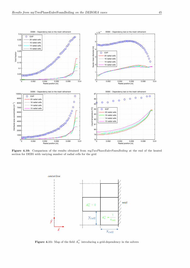
Results from myTwoPhaseEulerFoamBoiling on the DEBORA cases 45
0 0.002 0.004 0.006 0.008 0.010
0.05
0.1
0.15
0.2
0.25
0.3
0.35
0.4
Void
fra
ction
DEB5 − Dependency test on the mesh refinement
Radial position [m]
EXP
20 radial cells
16 radial cells
14 radial cells
10 radial cells
0 0.002 0.004 0.006 0.008 0.010
1
2
3
4
5
6x 10
−4
Saute
r m
ean d
iam
ete
r [m
]
DEB5 − Dependency test on the mesh refinement
Radial position [m]
EXP
20 radial cells
16 radial cells
14 radial cells
10 radial cells
0 0.002 0.004 0.006 0.008 0.010
1000
2000
3000
4000
5000
6000
7000
8000
9000
10000
Inte
rfacia
l are
a c
oncentr
ation [m
−1]
DEB5 − Dependency test on the mesh refinement
Radial position [m]
EXP
20 radial cells
16 radial cells
14 radial cells
10 radial cells
0 0.002 0.004 0.006 0.008 0.0178
79
80
81
82
83
84
85
86
87
Liq
uid
tem
pera
ture
[°C
]DEB5 − Dependency test on the mesh refinement
Radial position [m]
EXP
20 radial cells
16 radial cells
14 radial cells
10 radial cells
Figure 4.10: Comparison of the results obtained from myTwoPhaseEulerFoamBoiling at the end of the heatedsection for DEB5 with variying number of radial cells for the grid
Figure 4.11: Map of the field A′′′w introducing a grid-dependency in the solvers

46 Results
0 0.002 0.004 0.006 0.008 0.010
0.05
0.1
0.15
0.2
0.25
0.3
0.35
0.4
Void
fra
ction
DEB5 − Dependency test on the inlet value of the gas velocity
Radial position [m]
EXP
Present solver: Uain
=1.9 m/s
Present solver: Uain
=2.3 m/s
Present solver: Uain
=2.7 m/s
Present solver: Uain
=3 m/s
0 0.002 0.004 0.006 0.008 0.010
1
2
3
4
5
6x 10
−4
Saute
r m
ean d
iam
ete
r [m
]
DEB5 − Dependency test on the inlet value of the gas velocity
Radial position [m]
EXP
Present solver: Uain
=1.9 m/s
Present solver: Uain
=2.3 m/s
Present solver: Uain
=2.7 m/s
Present solver: Uain
=3 m/s
0 0.002 0.004 0.006 0.008 0.010
1000
2000
3000
4000
5000
6000
7000
8000
9000
10000
Inte
rfacia
l are
a c
oncentr
ation [m
−1]
DEB5 − Dependency test on the inlet value of the gas velocity
Radial position [m]
EXP
Present solver: Uain
=1.9 m/s
Present solver: Uain
=2.3 m/s
Present solver: Uain
=2.7 m/s
Present solver: Uain
=3 m/s
0 0.002 0.004 0.006 0.008 0.0178
79
80
81
82
83
84
85
86
87
Liq
uid
tem
pera
ture
[°C
]
DEB5 − Dependency test on the inlet value of the gas velocity
Radial position [m]
EXP
Present solver: Uain
=1.9 m/s
Present solver: Uain
=2.3 m/s
Present solver: Uain
=2.7 m/s
Present solver: Uain
=3 m/s
Figure 4.12: Comparison of the results obtained from myTwoPhaseEulerFoamBoiling at the end of the heatedsection for DEB5 with varying inlet gas velocity
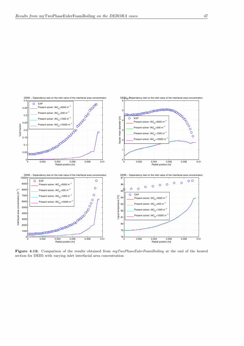
Results from myTwoPhaseEulerFoamBoiling on the DEBORA cases 47
0 0.002 0.004 0.006 0.008 0.010
0.05
0.1
0.15
0.2
0.25
0.3
0.35
0.4
Void
fra
ction
DEB5 − Dependency test on the inlet value of the interfacial area concentration
Radial position [m]
EXP
Present solver: IACin
=5000 m−1
Present solver: IACin
=200 m−1
Present solver: IACin
=1000 m−1
Present solver: IACin
=10000 m−1
0 0.002 0.004 0.006 0.008 0.010
1
2
3
4
5
6x 10
−4
Saute
r m
ean d
iam
ete
r [m
]
DEB5 − Dependency test on the inlet value of the interfacial area concentration
Radial position [m]
EXP
Present solver: IACin
=5000 m−1
Present solver: IACin
=200 m−1
Present solver: IACin
=1000 m−1
Present solver: IACin
=10000 m−1
0 0.002 0.004 0.006 0.008 0.010
1000
2000
3000
4000
5000
6000
7000
8000
9000
10000
Inte
rfacia
l are
a c
oncentr
ation [m
−1]
DEB5 − Dependency test on the inlet value of the interfacial area concentration
Radial position [m]
EXP
Present solver: IACin
=5000 m−1
Present solver: IACin
=200 m−1
Present solver: IACin
=1000 m−1
Present solver: IACin
=10000 m−1
0 0.002 0.004 0.006 0.008 0.0178
79
80
81
82
83
84
85
86
87
Liq
uid
tem
pera
ture
[°C
]
DEB5 − Dependency test on the inlet value of the interfacial area concentration
Radial position [m]
EXP
Present solver: IACin
=5000 m−1
Present solver: IACin
=200 m−1
Present solver: IACin
=1000 m−1
Present solver: IACin
=10000 m−1
Figure 4.13: Comparison of the results obtained from myTwoPhaseEulerFoamBoiling at the end of the heatedsection for DEB5 with varying inlet interfacial area concentration
48 Results
CHAPTER 5
DISCUSSION
5.1 On the myTwoPhaseEulerFoamAdiabatic solver
Even if the results given by this solver are satisfactory, it should be validated on a much wider range ofexperimental data with various flow conditions and using various geometries such as annulus, which wouldfirst require a new modeling of the wall lubrication force since the Tomiyama model only applies to pipe.In addition, one should also make sure that the results remain consistant when the solver is applied tothree-dimensional simulations.
The models used for the interfacial forces could be improved. The wall lubrication force model accordingto Tomiyama has two main inconveniencies: it is only applicable to pipes and it depends on their diameter.An option would be to implement the Frank model [11] in order to have a formulation with a wider rangeof applicability which would in the same time only depend on the distance to the wall. The virtual massforce has been implemented in this work but not activated in the momentum equation because it turned outto unstabilise the solver. This issue should be investigated too. However, it is acceptable not to considerthe virtual mass force since it reflects the influence of the accelerating fluid around a bubble and thereforevanishes when the steady-state is reached.
In order to better reproduce the intermediate void fraction profile, as the one observed at the higher measuringsection in DEDALE1101 (y/D = 155), one shoud probably adopt another approach for the interfacial areaconcentration. The present model is based on the assumption that there is only one possible size for bubbles ata given location in the pipe. Further research has been conducted on so called Multiple-Size-Group (MUSIG)approaches that allow to have different bubble sizes and therefore having as many transport equations asconsidered bubble sizes. With only two groups, Ishii and Kim [15] obtained encouraging results compared tothe present approach.
Other possible improvements concern the turbulence modeling. Instead of combining the Sato model with aclassic single phase k-ε turbulence model, one could follow the method described by Morel [25] and implementa modified k-ε model taking into account the turbulence caused by the bubbles on the liquid phase throughadditional source terms.
5.2 On the myTwoPhaseEulerFoamBoiling solver
As explained earlier, a great challenge and an issue which still remain to be resolved in this solver is howto properly model the heat flux density received by the liquid from the wall and implement it in a grid-independent manner. Imposing a uniform heat flux density may seem like a very simple problem in CFDbecause in most of the CFD software packages, the user just has to select the corresponding feature withouthaving to think about the way it is solved numerically.
A way to overcome this problem related to the treatment of the wall heat flux density could be to implementa dimensionless temperature wall function. Instead of adding a source term accounting for the wall heat inthe energy equation for near-wall cells, one may calculate the temperature in the node of the near-wall cells
49

50 Discussion
through a dimensionless temperature wall function, which would depend on the wall heat flux density. Apossible formulation is given by Kader [18]. This would at least solve the very high sensitivity of the solverto the grid resolution.
A related issue is how the boundary condition for the liquid enthalpy at the wall should be applied properly.The choice of a zeroGradient used in the simulations is questionable. In OpenFOAM, it might be commonto impose a uniform enthalpy gradient at the wall, according to the Fourier law, implying that conduction isthe main heat transfer mechanism between the wall and the liquid. But this in not valid in our case since theheat transfer phenomenon is governed by other mechanisms, as can be seen from the heat flux partitioning.However, tests have been performed imposing a non-zero uniform gradient at the wall and the results werealmost identical.
CHAPTER 6
CONCLUSIONS
According to many experts, nuclear power will play an important role in tomorrow’s energy supply. Thisopinion is essentially motivated by global warming and the depletion of fossil resources. However, thistechnology still faces sometimes the public opinion’s reluctancy based mostly on safety issues and storage ofnuclear waste. A few safety issues in the nuclear industry are related to subcooled nucleate boiling. Thisphenomenon designates the first boiling regime: liquid evaporates at a heated wall, generating bubbles whichthen migrate to the subcooled liquid and condensate, heating the latter up. This regime normally occursin the lower part of BWR fuel bundles and could also occur at the highest part of a PWR core. For aheat flux equal to the Critical Heat Flux (CHF), one leaves the nucleate boing regime. This transition iscalled Departure From Nucleate boiling and marks a very sudden increase in the fuel clad temperature thatmay lead to structural damage and consequently to infringement to the defence-in-depth principle. Anotherreason why one would like to be able to predict this phenomenon more accurately is that the void generatedin a BWR core will affect the reactivity of the reactor, and in a PWR it leads to a so-called axial offsetanomaly due to the deposition of lithium borate. Therefore, accurate models of subcooled nucleate boilingare of major interest. So far, the codes used for this purpose are old system level codes and there is a crucialneed of improved three-dimensional models in CFD.
In this study, subcooled nucleate boiling in vertical pipes has been modeled within the OpenFOAM frame-work. OpenFOAM is a relatively new CFD software package, quite different from the most common com-mercial codes. Its user-friendliness is limited since it does not contain any graphical interface. Besides, thenumber of existing models that comes with it is limited. However, this code has a huge potential. Theimplementation of equations is transparent and the source code is rather easily understandable, and as itopen source, the code is modifiable, allowing the user to implement customised models. Therefore, this codecan continuously be improved by the users community and does not rely on any release by a company.
The modelling of subcooled nucleate boiling has been carried out in two steps. In the first step, a solvernamed myTwoPhaseEulerFoamAdiabatic has been implemented to simulate adiabatic bubbly flow using aEulerian-Eulerian approach. In this solver, the mass and momentum conservation equations are solved forboth phases and an interfacial area transport equation has been implemented. Additionally, the turbulencehas been neglected in the gas phase, and modeled for the liquid phase using a classic k-ε model in combinationwith standard wall functions. A bubble induced turbulent viscosity has been implemented according to theproposed model by Sato. Special care has been taken for the interfacial forces and the following modelshave been chosen: the Ishii-Zuber drag, the Tomiyama lift, the Tomiyama wall lubrication and the Gosmanturbulent dispersion forces. The Zuber virtual mass force has been implemented but it was not activatedwhile solving the momentum equations in the present studies. Furthermore, two different models, namelythe Hibiki and Ishii model as well as the Yao and Morel model, have been implemented for the coalescenceand breakup source terms appearing in the interfacial area concentration transport equation. Either one orthe other can be selected by the user.
Then, a solver called myTwoPhaseEulerFoamBoiling has been developed based on the previous one. In orderto take into account nucleation at the heated pipe wall and condensation in the subcooled liquid, whileassuming that the gas remains at the saturated conditions, only one energy conservation equation has beenincluded - the one for the liquid phase. Furthermore phase change terms have been introduced in the mass-and momentum conservation equations, as well as in the interfacial area concentration transport equation.
51

52 Conclusions
The turbulence modeling has not been modified.
The solver myTwoPhaseEulerFoamAdiabatic has been tested and validated again two data sets extractedfrom the DEDALE experimental database. The results are satisfactory since the void fraction wall peakobserved experimentally is captured and the predicted values both at the peak and in the core of the pipe arereasonably accurate. The calculated position of the peak could however be improved. It is currently slightlytoo far from the wall but this might be related to the profiles applied at the inlet. In the simulations, theyhave been chosen uniform because there is a lack of information concerning the radial profiles at the inletand only cross-section average values could be found in the literature. However in reality, the flow will bepartially developed. The results also show that the Hibiki and Ishii model for the coalescence and breakupterms appearing in the interfacial area equation leads to more accurate results than the Yao and Morel modelat intermediate channel heights but it cannot capture the axial evolution of the radial profiles. It is believedthat this is related to the fact that the numerical constants used by Yao and Morel were derived analitycally,whereas those used by Hibiki and Ishii were fitted on experimental data.
With regards to the comparison between the results obtained from the myTwoPhaseEulerFoamBoiling solverand those from the experiment, one must admit that some further improvements have to be done. The trendsof the distributions of many parameters are physically reasonable, as for example, the temperature increasesaxially and decreases radially away fromm the wall, but the results are too inaccurate. The boiling sub-model is believed to be properly implemented because the key parameter, the bubble detachment diameter,is predicted with a relatively good precision. It has also been tested (but not shown in this report) to removethe condensation rate but the void fraction predictions were still far too low. Therefore, it is quite plausiblethat the reason for these discrepancies lies in the energy equation. This hypothesis is strengthened by lookingat the void fraction and liquid temperature predictions, which are highly underestimated. Since the rise inkinetic energy of the fluid between the inlet and the outlet is not so important, this implies that part of theenergy flux from the wall is lost. This issue regarding the proper treatment of the wall heat flux density fornear-wall cells is the origin of the grid sensitivity which has been noticed. However, the work which has beendone on myTwoPhaseEulerFoamBoiling remains valuable. The solvers code is stable, the solution procedureis well defined and its architecture properly constructed with different classes for different physical entitiessuch as interfacial forces or coalescence and breakup mechanisms. Besides, its robustness has been provenby investigating its insensitivity to the inlet gas velocity and the inlet interfacial area concentration, whichdo not have any physical significance when water is subcooled.
There are several aspects that need to be addressed in future work on this topic. In order to improve themyTwoPhaseEulerFoamAdiabatic solver, one could first focus on the interfacial forces. Using the Frank[11] wall lubrication model would make this force valid for other geometries than pipes and make thisforce geometry-independent. Then considering a Multi-Size-Group (MUSIG), as was done by Ishii andKim [15] for the modeling of the bubble transport phenomena instead of the one-group interfacial areaconcentration equation would perhaps capture the axial evolution of the parameters radial profiles and givebetter predictions of the bubbly-to-slug transition. Finally, modified k-ε equations dedicated to two-phaseflows could be implemented, as for instance the one described by Morel [25].
Regarding myTwoPhaseEulerFoamBoiling, whose results are not as satisfactory, the challenge is most cer-tainly how to properly implement the heat flux applied to the near-wall cells in a grid-independent manner.The approach described by Kader [18] based on using a temperature wall function for near wall cells couldbe a solution. Therefore the heat flux should probably be removed from the enthalpy equation and this tem-perature wall function used for the calculation of the liquid enthalpy in the near-wall cells instead. Besidesone should investigate the boundary condition to apply to the enthalpy at the wall.
BIBLIOGRAPHY
[1] H. Anglart. Thermal-Hydraulics in Nuclear Systems (KTH, Stockholm, 2008).
[2] Inc. ANSYS. ANSYS CFX-Solver Theory Guide, 12.1 edn., November 2009.
[3] S.P. Antal et al. Analysis of phase distribution in fully developed laminar bubbly two-phase flow. Inter-national Journal of Multiphase Flow, 7:pp. 635–652, 1991.
[4] D. Bestion and P. Peturaud. Deliverable D2.2.1: Review of the existing data basis for the validation ofmodels for CHF. 6th EURATOM framework programme, NURESIM-SP2-TH, 2006.
[5] J. Boree et al. Ecoulements diphasiques eau-vapeur avec changement de phase. Tech. rep., Rapportintermediaire IMFT- Interface, 1995.
[6] J. Boussinesq. Theorie de l’ecoulement tourbillonnant et tumultueux des liquides dans les lits rectilignesa grandes sections (Gauthier-Villars, Paris, 1897).
[7] W.C. Ceumern-Lindenstjerna. Bubble departure diameter and release frequencies during nucleate poolboiling of water and aqueous nacl solutions. Heat Transfer in boiling, 1977.
[8] J.M. Delhaye. Some issues related to the modelling of interfacial areas in gas–liquid flows, part ii:modelling the source terms for dispersed flows. C. R. Acad. Sci. Paris, t. 329(Serie II b):pp. p. 473–486,2001.
[9] M. DelValle and D.B.R Kenning. Subcooled flow boiling at high heat flux. International Journal of Heatand Mass Transfer, 28:pp. 1907–1920, 1985.
[10] D.A. Drew and R.T. Lahey. The virtual mass and lift force on a sphere in rotating and straining inviscidflow. International Journal of Multiphase Flow, 13:pp. 113–121, 1987.
[11] Th. Frank. Advances in computational fluid dynamics (cfd) of 3-dimensional gas–liquid multiphase flows.In NAFEMS Seminar ”Simulation of Complex Flows (CFD)”, pp. 1–18 (Wiesbaden, Germany, 2005).
[12] A.D. Gosman et al. Multidimensional modeling of turbulent two-phase flow in stirred vessels. AIChEJournal, 38:pp. 1946–1956, 1992.
[13] T. Hibiki and M. Ishii. Development of one-group interfacial area transport equation in bubbly flowsystems. International Journal of Heat and Mass Transfer, 45:pp. 2351–2372, 2002.
[14] M. Ishii and S. Kim. Micro four-sensor probe measurement of interfacial area transport for bubbly flowin round pipes. Nuclear Engineering and Design, 205:pp. 2711–2726, 2001.
[15] M. Ishii and S. Kim. Development of one-group and two- group interfacial area transport equation.Nuclear Science and Engineering, 3:pp. 257–273, 2004.
[16] W.H. Jens and P.A. Lottes. Analysis of heat transfer burnout, pressure drop, and density data forhigh-pressure water. Tech. rep., Argonne National Laboratories, 1951.
53
54 Bibliography
[17] M. Jischa and H.B. Rieke. About the prediction of turbulent prandtl and schmidt numbers from modeledtransport equations. International Journal of Heat and Mass Transfer, 22(11):pp. 1547–1555, 1979. ISSN0017-9310. doi:DOI:10.1016/0017-9310(79)90134-0.
[18] B.A. Kader. Temperature and concentration profiles in fully turbulent boundary layers. InternationalJournal of Heat and Mass Transfer, 24:pp. 1541–1544, 1981.
[19] N. Kurul and M.Z. Podowski. On the modeling of multidimensional effects in boiling channels. Proceed-ings of the 27th National Heat Transfer Conference, June 1991.
[20] M. Lemmert and J.M Chawla. Influence of flow velocity on surface boiling heat transfer coefficient. HeatTransfer in Boiling, pp. 237–247, 1977.
[21] OpenCFD Limited. OpenFOAM Programmer’s C++ Documentation.http://foam.sourceforge.net/doc/Doxygen/html/, 2011.
[22] OpenCFD Limited. OpenFOAM User Guide. http://www.openfoam.com/docs/user/, 2011.
[23] M. Lopez De Bertodano and D. Prabhudharwadkar. Computational fluid dynamics, pp. 420–444. CFDTwo Fluid Model for Adiabatic and Boiling Bubbly Flows in Ducts (InTech, 2010).
[24] E. Manon. Contribution a lanalyse et a la modelisation des ecoulements bouillants sous-satures dansles conditions des Reacteurs a Eau sous Pression en presence d’ebullition. Ph.D. thesis, Ecole CentraleParis, 2000.
[25] C. Morel. An order of magnitude analysis of the two-phase k–e model. International Journal of FluidMechanics Research, 22:pp. 21–44, 1995.
[26] H. Rusche. Computational fluid dynamics of dispersed two-phase flows at high phase fractions. Ph.D.thesis, Imperial College, London, 2002.
[27] Y. Sato et al. Momentum and heat transfer in two-phase bubbly flow. International Journal of MultiphaseFlow, 7:pp. 167–178, 1981.
[28] B. Stroustrup. The C++ programming language (Addison-Wesley, 1991), second edition edn. ISBN0-201-53992-6.
[29] X. Pedruelo Tapia. Modeling of wind flow over complex terrain using OpenFOAM. Master’s thesis,University of Gavle, Sweden, 2009.
[30] R. Thiele. Direct Contact Condensation with OpenFOAM. Master’s thesis, KTH, Stockholm, 2010.
[31] J.R.S. Thom et al. Boiling in subcooled water during flow up heated tubes or annuli. In Symposiumon Boiling Heat Transfer in Steam Generating Units and Heat Exchangers (Institute of MechanicalEngineers, London, 1965).
[32] V.I. Tolubinsky and D.M. Kostanchuk. Vapor bubble growth rate and heat transfer intensity at subcooledwater boiling. In 4th International Heat Transfer Conference (1970).
[33] A. Tomiyama. Struggle with computational bubble dynamics. Third International Conference on Multi-phase Flow, 1998.
[34] T.Salnikova. TWO-PHASE CFD ANALYSES IN FUEL ASSEMBLY SUB-CHANNELS OF PRES-SURIZED WATER REACTORS UNDER SWIRL CONDITIONS. Ph.D. thesis, Technische UniversitatDresden, 2008.
[35] H.C. Unal. Maximum bubble diameter, maximum bubble-growth rate during the sub- cooled nucleate flowboiling of water up to 17.7 mn/m2. International Journal of Heat and Mass Transfer, 19:pp. 643–649,1976.
[36] R.M. Wellek et al. Shapes of liquid drops moving in liquid media. AIChE Journal, 12:pp. 854–860, 1966.
[37] K. Wolfert. Non-equilibrium mass transfer between liquid and vapor phases during depressurizationprocesses in transient two-phase flow. In Proc. 2nd CSNI Specialists meeting, vol. 2, pp. 1377–1387(Paris, 1978).
[38] Q. Wu et al. One-group interfacial area transport in vertical bubble flow. International Journal of Heatand Mass Transfer, 41:pp. 1103–1112, 1998.

Bibliography 55
[39] W. Yao and C. Morel. Volumetric interfacial area prediction in upward bubbly two-phase flow. Interna-tional Journal of Heat and Mass Transfer, 47:pp. 307–328, 2004.
[40] N. Zuber. On the dispersed two-phase flow in the laminar flow regime. Chemical Engineering Science,19(11):pp. 897–917, 1964. ISSN 0009-2509. doi:DOI:10.1016/0009-2509(64)85067-3.

56 Bibliography
APPENDIX A
INSTALLATION GUIDELINES
Here are a few guidelines which will help you to install the new solvers myTwoPhaseEulerFoamAdiabaticand myTwoPhaseEulerFoamBoiling and use them on the provided cases. These guidelines are given formyTwoPhaseEulerFoamAdiabatic but the procedure is identical for myTwoPhaseEulerFoamBoiling
1) Copying the cases
• Enter the folder run included on the attached DVD
• Copy the folder myTwoPhaseEulerFoamAdiabatic (which contains the different cases on which thesolver can be tested) and paste it in the run directory of your local workspace (in my case for instance:/home/michta/OpenFOAM/michta-1.7.x/run). If this run directory does not exist yet, create it.
2) Copying the solver
• Enter the folder solvers included on the attached DVD
• Copy the folder myTwoPhaseEulerFoamAdiabatic (which contains the solver) and paste it in thesolvers directory of your local workspace (in my case for instance: /home/michta/OpenFOAM/michta-1.7.x/applications/solvers). If this solvers directory does not exist yet, create it.
3) Libraries linking and compiling
• Open a terminal that you will use from now on
• Go into the myTwoPhaseEulerFoamAdiabatic solver folder of your local workspace (in my case :/home/michta/OpenFOAM/michta-1.7.x/applications/myTwoPhaseEulerFoamAdiabatic) and performsuccessively the following steps:
– Go into the phaseModel folder and compile it using the command wmake libso (it is essential tocompile this submodel first!)
– Go into the breakupAndCoalescenceModels folder and compile it using the command wmake libso
– Go into the interfacialModels folder and compile it using the command wmake libso
• Being located in your myTwoPhaseEulerFoamAdiabatic solver folder, compile it by using the commandwmake.
4) Running a case
• Still using the terminal, locate the folder of the case you want to run
• Then simply type the name of the solver you want to use for this case in the terminal. Here we willjust use the command myTwoPhaseEulerFoamAdiabatic.
57
58 Installation guidelines
5) Postprocessing
• In order to postprocess your simulation, using ParaView, you must first be located (still using theterminal) in the folder of the case you want to postprocess
• Then simply use the command paraFoam.
APPENDIX B
SOURCE CODE: MAIN PROGRAM
001: /*--–-–-–-–-–-–-–-–-–-–-–-–-–-–-–-–-–-–-–-–-–-–-–-–--*\002: ========= |003: \\ / F ield | OpenFOAM: The Open Source CFD Toolbox004: \\ / O peration |005: \\ / A nd | Copyright (C) 1991-2010 OpenCFD Ltd.006: \\/ M anipulation |007: --–-–-–-–-–-–-–-–-–-–-–-–-–-–-–-–-–-–-–-–-–-–-–-–-–-–008: License009: This file is part of OpenFOAM.010:011: OpenFOAM is free software: you can redistribute it and/or modify it012: under the terms of the GNU General Public License as published by013: the Free Software Foundation, either version 3 of the License, or014: (at your option) any later version.015:016: OpenFOAM is distributed in the hope that it will be useful, but WITHOUT017: ANY WARRANTY; without even the implied warranty of MERCHANTABILITY or018: FITNESS FOR A PARTICULAR PURPOSE. See the GNU General Public License019: for more details.020:021: You should have received a copy of the GNU General Public License022: along with OpenFOAM. If not, see <http://www.gnu.org/licenses/>.023:024: Application025: myTwoPhaseEulerFoamBoiling026:027: Author028: Edouard Michta029: [email protected]:031: Description032: Solver for modeling of subcooled nucleate boiling033:034: Solver based on twoPhaseEulerFoam, accounting for phase change due to035: nucleation at a heated wall and subsequent condensation in the bulk liquid036:037: Equations solved:038: - mass and momentum conservation equation for both phases039: - energy equation for the liquid phase040: - one-group interfacial area concentration transport equation041: - if ””turbulence”” is switched on: RANS classic k-epsilon model + standard
59

60 Source code: main program
042: wall functions043:044: \*--–-–-–-–-–-–-–-–-–-–-–-–-–-–-–-–-–-–-–-–-–-–-–-–--*/045:046: #include ”fvCFD.H”047: #include ”nearWallDist.H”048: #include ”wallFvPatch.H”049: #include ”Switch.H”050:051: #include ”IFstream.H”052: #include ”OFstream.H”053:054: #include ”phaseModel.H”055: #include ”dragModel.H”056: #include ”liftModel.H”057: #include ”virtualMassModel.H”058: #include ”turbulentDispersionModel.H”059: #include ”wallLubricationModel.H”060: #include ”breakupModel.H”061: #include ”coalescenceModel.H”062:063: // * * * * * * * * * * * * * * * * * * * * * * * * * * * * * * * * * * * * * //064:065: int main(int argc, char *argv[])066: {067: #include ”setRootCase.H”068:069: #include ”createTime.H”070: #include ”createMesh.H”071: #include ”readGravitationalAcceleration.H”072: #include ”readEnvironmentalProperties.H”073: #include ”createFields.H”074: #include ”initContinuityErrs.H”075: #include ”readTimeControls.H”076: #include ”CourantNo.H”077: #include ”setInitialDeltaT.H”078:079: // * * * * * * * * * * * * * * * * * * * * * * * * * * * * * * * * * * * //080:081: Info<< ”\nStarting time loop\n” << endl;082:083: while (runTime.run())084: {085: #include ”readTwoPhaseEulerFoamControls.H”086: #include ”CourantNos.H”087: #include ”setDeltaT.H”088:089: runTime++;090: Info<< ”Time = ” << runTime.timeName() << nl << endl;091:092: #include ”condensationModel.H”093: #include ”evaporationModel.H”094: #include ”alphaEqn.H”095: #include ”IACEqn.H”096:097: // --- Outer-corrector loop098: for (int oCorr=0; oCorr<nCorr; oCorr++)099: {100:101: #include ”interMomentumForces.H”

61
102: #include ”UEqns.H”103:104: // --- PISO loop105: for (int corr=0; corr<nCorr; corr++)106: {107: #include ”pEqn.H”108: if (correctAlpha && corr<nCorr-1)109: {110: #include ”alphaEqn.H”111: #include ”IACEqn.H”112: }113: }114:115: #include ”DDtU.H”116: #include ”kEpsilon.H”117: #include ”HEqns.H”118: }119:120: #include ”write.H”121:122: Info<< ”ExecutionTime = ” << runTime.elapsedCpuTime() << ” s”123: << ” ClockTime = ” << runTime.elapsedClockTime() << ” s”124: << nl << endl;125: }126:127: Info<< ”End\n” << endl;128:129: return 0;130: }131:132:133: // ************************************************************************* //134:

62 Source code: main program
APPENDIX C
SOURCE CODE: ISHII-ZUBER DRAG
001: /*--–-–-–-–-–-–-–-–-–-–-–-–-–-–-–-–-–-–-–-–-–-–-–-–--*\002: ========= |003: \\ / F ield | OpenFOAM: The Open Source CFD Toolbox004: \\ / O peration |005: \\ / A nd | Copyright (C) 1991-2007 OpenCFD Ltd.006: \\/ M anipulation |007: --–-–-–-–-–-–-–-–-–-–-–-–-–-–-–-–-–-–-–-–-–-–-–-–-–-–008: License009: This file is part of OpenFOAM.010:011: OpenFOAM is free software; you can redistribute it and/or modify it012: under the terms of the GNU General Public License as published by the013: Free Software Foundation; either version 2 of the License, or (at your014: option) any later version.015:016: OpenFOAM is distributed in the hope that it will be useful, but WITHOUT017: ANY WARRANTY; without even the implied warranty of MERCHANTABILITY or018: FITNESS FOR A PARTICULAR PURPOSE. See the GNU General Public License019: for more details.020:021: You should have received a copy of the GNU General Public License022: along with OpenFOAM; if not, write to the Free Software Foundation,023: Inc., 59 Temple Place, Suite 330, Boston, MA 02111-1307 USA024:025: \*--–-–-–-–-–-–-–-–-–-–-–-–-–-–-–-–-–-–-–-–-–-–-–-–--*/026:027: #include ”Ishii.H”028: #include ”addToRunTimeSelectionTable.H”029:030: // * * * * * * * * * * * * * * Static Data Members * * * * * * * * * * * * * //031:032: namespace Foam033: {034: defineTypeNameAndDebug(Ishii, 0);035:036: addToRunTimeSelectionTable037: (038: dragModel,039: Ishii,040: dictionary041: );
63

64 Source code: Ishii-Zuber drag
042: }043:044:045: // * * * * * * * * * * * * * * * * Constructors * * * * * * * * * * * * * * //046:047: Foam::Ishii::Ishii048: (049: const dictionary& interfaceDict,050: const volScalarField& alpha,051: const phaseModel& phasea,052: const phaseModel& phaseb053: )054: :055: dragModel(interfaceDict, alpha, phasea, phaseb)056: {}057:058:059: // * * * * * * * * * * * * * * * * Destructor * * * * * * * * * * * * * * * //060:061: Foam::Ishii::˜Ishii()062: {}063:064:065: // * * * * * * * * * * * * * * * Member Functions * * * * * * * * * * * * * //066:067: Foam::tmp<Foam::volScalarField> Foam::Ishii::AD068: (069: const volScalarField& Ur,070: const volScalarField& DS071:072: ) const073: {074:075: dimensionedScalar plusDS076: (077: ”plusDS”,078: dimensionSet(0, 1, 0, 0, 0, 0, 0),079: scalar (1.0e-6)080: );081:082: scalar alphaMax = 0.52;083:084: dimensionedScalar muStar = (phasea .rho()*phasea .nu()+0.4*phaseb .rho()085: *phaseb .nu())/(phasea .rho()*phasea .nu()+phaseb .rho()*phaseb .nu());086: volScalarField nuMix = phaseb .nu()*pow((scalar(1.0)-alpha /alphaMax),087: -2.5*alphaMax*muStar);088: volScalarField ReMix = max(Ur*DS/nuMix, scalar(1.0e-3));089: volScalarField Cd = 24.0*(scalar(1) + 0.15*pow(ReMix, 0.687))/(ReMix+0.001);090:091: forAll(ReMix, celli)092: {093: if(ReMix[celli] > 1000.0)094: {095: Cd[celli] = 0.44;096: }097: }098:099: return 0.75*Cd*phaseb .rho()*Ur/(DS+plusDS);100: }101:

65
102:103: // ************************************************************************* //104:

66 Source code: Ishii-Zuber drag
APPENDIXD
SOURCE CODE: TOMIYAMA LIFT
001: /*--–-–-–-–-–-–-–-–-–-–-–-–-–-–-–-–-–-–-–-–-–-–-–-–--*\002: ========= |003: \\ / F ield | OpenFOAM: The Open Source CFD Toolbox004: \\ / O peration |005: \\ / A nd | Copyright (C) 1991-2007 OpenCFD Ltd.006: \\/ M anipulation |007: --–-–-–-–-–-–-–-–-–-–-–-–-–-–-–-–-–-–-–-–-–-–-–-–-–-–008: License009: This file is part of OpenFOAM.010:011: OpenFOAM is free software; you can redistribute it and/or modify it012: under the terms of the GNU General Public License as published by the013: Free Software Foundation; either version 2 of the License, or (at your014: option) any later version.015:016: OpenFOAM is distributed in the hope that it will be useful, but WITHOUT017: ANY WARRANTY; without even the implied warranty of MERCHANTABILITY or018: FITNESS FOR A PARTICULAR PURPOSE. See the GNU General Public License019: for more details.020:021: You should have received a copy of the GNU General Public License022: along with OpenFOAM; if not, write to the Free Software Foundation,023: Inc., 59 Temple Place, Suite 330, Boston, MA 02111-1307 USA024:025: \*--–-–-–-–-–-–-–-–-–-–-–-–-–-–-–-–-–-–-–-–-–-–-–-–--*/026:027: #include ”liftTomiyama.H”028: #include ”addToRunTimeSelectionTable.H”029:030: // * * * * * * * * * * * * * * Static Data Members * * * * * * * * * * * * * //031:032: namespace Foam033: {034: defineTypeNameAndDebug(liftTomiyama, 0);035:036: addToRunTimeSelectionTable037: (038: liftModel,039: liftTomiyama,040: dictionary041: );
67
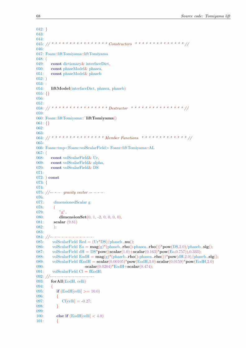
68 Source code: Tomiyama lift
042: }043:044:045: // * * * * * * * * * * * * * * * * Constructors * * * * * * * * * * * * * * //046:047: Foam::liftTomiyama::liftTomiyama048: (049: const dictionary& interfaceDict,050: const phaseModel& phasea,051: const phaseModel& phaseb052: )053: :054: liftModel(interfaceDict, phasea, phaseb)055: {}056:057:058: // * * * * * * * * * * * * * * * * Destructor * * * * * * * * * * * * * * * //059:060: Foam::liftTomiyama::˜liftTomiyama()061: {}062:063:064: // * * * * * * * * * * * * * * * Member Functions * * * * * * * * * * * * * //065:066: Foam::tmp<Foam::volScalarField> Foam::liftTomiyama::AL067: (068: const volScalarField& Ur,069: const volScalarField& alpha,070: const volScalarField& DS071:072: ) const073: {074:075: //--–-–-– gravity vector --–-–-–-–076:077: dimensionedScalar g078: (079: ”g”,080: dimensionSet(0, 1, -2, 0, 0, 0, 0),081: scalar (9.81)082: );083:084: //--–-–-–-–-–-–-–-–-–-–-–-–085: volScalarField Red = (Ur*DS)/phaseb .nu();086: volScalarField Eo = mag(g)*(phaseb .rho()-phasea .rho())*pow(DS,2.0)/phaseb .sig();087: volScalarField dH = DS*pow((scalar(1.0)+scalar(0.163)*pow(Eo,0.757)),0.333);088: volScalarField EodH = mag(g)*(phaseb .rho()-phasea .rho())*pow(dH,2.0)/phaseb .sig();089: volScalarField fEodH = scalar(0.00105)*pow(EodH,3.0)-scalar(0.0159)*pow(EodH,2.0)090: -scalar(0.0204)*EodH+scalar(0.474);091: volScalarField Cl = fEodH;092: //--–-–-–-–-–-–-–-–-–-–-–-–093: forAll(EodH, celli)094: {095: if (EodH[celli] >= 10.0)096: {097: Cl[celli] = -0.27;098: }099:100: else if (EodH[celli] < 4.0)101: {

69
102: Cl[celli] = min(scalar(0.288)*tanh((scalar(0.121)*Red[celli])),fEodH[celli]);103: }104: }105:106: return Cl*phaseb .rho();107:108: }109:110: // ************************************************************************* //111:

70 Source code: Tomiyama lift
APPENDIX E
SOURCE CODE: TOMIYAMA WALL LUBRICATION
001: /*--–-–-–-–-–-–-–-–-–-–-–-–-–-–-–-–-–-–-–-–-–-–-–-–--*\002: ========= |003: \\ / F ield | OpenFOAM: The Open Source CFD Toolbox004: \\ / O peration |005: \\ / A nd | Copyright (C) 1991-2007 OpenCFD Ltd.006: \\/ M anipulation |007: --–-–-–-–-–-–-–-–-–-–-–-–-–-–-–-–-–-–-–-–-–-–-–-–-–-–008: License009: This file is part of OpenFOAM.010:011: OpenFOAM is free software; you can redistribute it and/or modify it012: under the terms of the GNU General Public License as published by the013: Free Software Foundation; either version 2 of the License, or (at your014: option) any later version.015:016: OpenFOAM is distributed in the hope that it will be useful, but WITHOUT017: ANY WARRANTY; without even the implied warranty of MERCHANTABILITY or018: FITNESS FOR A PARTICULAR PURPOSE. See the GNU General Public License019: for more details.020:021: You should have received a copy of the GNU General Public License022: along with OpenFOAM; if not, write to the Free Software Foundation,023: Inc., 59 Temple Place, Suite 330, Boston, MA 02111-1307 USA024:025: \*--–-–-–-–-–-–-–-–-–-–-–-–-–-–-–-–-–-–-–-–-–-–-–-–--*/026:027: #include ”wallLubricationTomiyama.H”028: #include ”addToRunTimeSelectionTable.H”029:030: // * * * * * * * * * * * * * * Static Data Members * * * * * * * * * * * * * //031:032: namespace Foam033: {034: defineTypeNameAndDebug(wallLubricationTomiyama, 0);035:036: addToRunTimeSelectionTable037: (038: wallLubricationModel,039: wallLubricationTomiyama,040: dictionary041: );
71
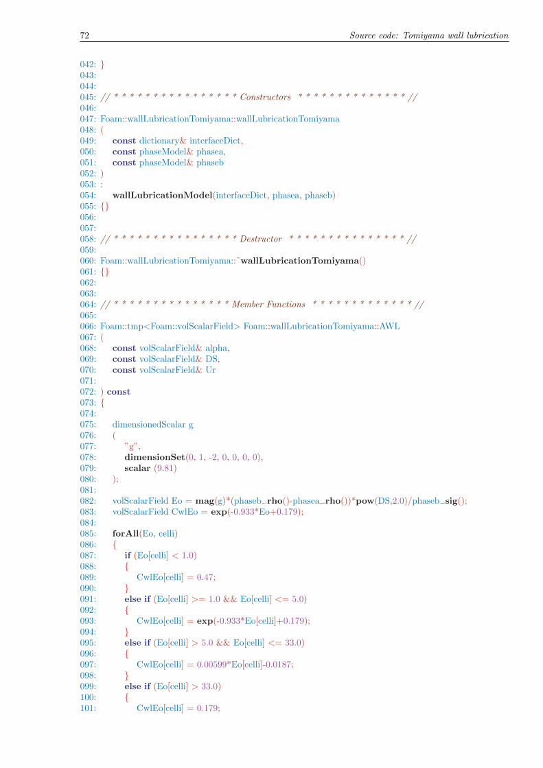
72 Source code: Tomiyama wall lubrication
042: }043:044:045: // * * * * * * * * * * * * * * * * Constructors * * * * * * * * * * * * * * //046:047: Foam::wallLubricationTomiyama::wallLubricationTomiyama048: (049: const dictionary& interfaceDict,050: const phaseModel& phasea,051: const phaseModel& phaseb052: )053: :054: wallLubricationModel(interfaceDict, phasea, phaseb)055: {}056:057:058: // * * * * * * * * * * * * * * * * Destructor * * * * * * * * * * * * * * * //059:060: Foam::wallLubricationTomiyama::˜wallLubricationTomiyama()061: {}062:063:064: // * * * * * * * * * * * * * * * Member Functions * * * * * * * * * * * * * //065:066: Foam::tmp<Foam::volScalarField> Foam::wallLubricationTomiyama::AWL067: (068: const volScalarField& alpha,069: const volScalarField& DS,070: const volScalarField& Ur071:072: ) const073: {074:075: dimensionedScalar g076: (077: ”g”,078: dimensionSet(0, 1, -2, 0, 0, 0, 0),079: scalar (9.81)080: );081:082: volScalarField Eo = mag(g)*(phaseb .rho()-phasea .rho())*pow(DS,2.0)/phaseb .sig();083: volScalarField CwlEo = exp(-0.933*Eo+0.179);084:085: forAll(Eo, celli)086: {087: if (Eo[celli] < 1.0)088: {089: CwlEo[celli] = 0.47;090: }091: else if (Eo[celli] >= 1.0 && Eo[celli] <= 5.0)092: {093: CwlEo[celli] = exp(-0.933*Eo[celli]+0.179);094: }095: else if (Eo[celli] > 5.0 && Eo[celli] <= 33.0)096: {097: CwlEo[celli] = 0.00599*Eo[celli]-0.0187;098: }099: else if (Eo[celli] > 33.0)100: {101: CwlEo[celli] = 0.179;

73
102: }103:104: }105:106: return 0.5*CwlEo*phaseb .rho()*pow(Ur,2.0)*DS;107: //*pos(alpha-scalar(0.0001));108: }109:110:111: // ************************************************************************* //112:
74 Source code: Tomiyama wall lubrication
APPENDIX F
SOURCE CODE: GOSMAN TURBULENT DISPERSION
001: /*--–-–-–-–-–-–-–-–-–-–-–-–-–-–-–-–-–-–-–-–-–-–-–-–--*\002: ========= |003: \\ / F ield | OpenFOAM: The Open Source CFD Toolbox004: \\ / O peration |005: \\ / A nd | Copyright (C) 1991-2007 OpenCFD Ltd.006: \\/ M anipulation |007: --–-–-–-–-–-–-–-–-–-–-–-–-–-–-–-–-–-–-–-–-–-–-–-–-–-–008: License009: This file is part of OpenFOAM.010:011: OpenFOAM is free software; you can redistribute it and/or modify it012: under the terms of the GNU General Public License as published by the013: Free Software Foundation; either version 2 of the License, or (at your014: option) any later version.015:016: OpenFOAM is distributed in the hope that it will be useful, but WITHOUT017: ANY WARRANTY; without even the implied warranty of MERCHANTABILITY or018: FITNESS FOR A PARTICULAR PURPOSE. See the GNU General Public License019: for more details.020:021: You should have received a copy of the GNU General Public License022: along with OpenFOAM; if not, write to the Free Software Foundation,023: Inc., 59 Temple Place, Suite 330, Boston, MA 02111-1307 USA024:025: \*--–-–-–-–-–-–-–-–-–-–-–-–-–-–-–-–-–-–-–-–-–-–-–-–--*/026:027: #include ”Gosman.H”028: #include ”addToRunTimeSelectionTable.H”029:030: // * * * * * * * * * * * * * * Static Data Members * * * * * * * * * * * * * //031:032: namespace Foam033: {034: defineTypeNameAndDebug(Gosman, 0);035:036: addToRunTimeSelectionTable037: (038: turbulentDispersionModel,039: Gosman,040: dictionary041: );
75

76 Source code: Gosman turbulent dispersion
042: }043:044:045: // * * * * * * * * * * * * * * * * Constructors * * * * * * * * * * * * * * //046:047: Foam::Gosman::Gosman048: (049: const dictionary& interfaceDict,050: const phaseModel& phasea,051: const phaseModel& phaseb052: )053: :054: turbulentDispersionModel(interfaceDict, phasea, phaseb)055: {}056:057:058: // * * * * * * * * * * * * * * * * Destructor * * * * * * * * * * * * * * * //059:060: Foam::Gosman::˜Gosman()061: {}062:063:064: // * * * * * * * * * * * * * * * Member Functions * * * * * * * * * * * * * //065:066: Foam::tmp<Foam::volScalarField> Foam::Gosman::ATD067: (068: const volScalarField& Ur,069: const volScalarField& nutb,070: const volScalarField& DS,071: const volScalarField& alpha072:073: ) const074: {075:076: scalar sigmat = 0.9;077:078: dimensionedScalar plusDS079: (080: ”plusDS”,081: dimensionSet(0, 1, 0, 0, 0, 0, 0),082: scalar (1.0e-6)083: );084:085: scalar alphaMax = 0.52;086:087: //If calculated from Ishii drag088:089: dimensionedScalar muStar = (phasea .rho()*phasea .nu()+0.4*phaseb .rho()*phaseb .nu())090: /(phasea .rho()*phasea .nu()+phaseb .rho()*phaseb .nu());091: volScalarField nuMix = phaseb .nu()*pow((scalar(1.0)-alpha/alphaMax),092: -2.5*alphaMax*muStar);093: volScalarField ReMix = max(Ur*DS/nuMix, scalar(1.0e-3));094: volScalarField Cd = 24.0*(scalar(1) + 0.15*pow(ReMix, 0.687))/(ReMix+0.001);095:096: forAll(ReMix, celli)097: {098: if(ReMix[celli] > 1000.0)099: {100: Cd[celli] = 0.44;101: }
77
102: }103:104:105: return scalar(0.75)*Cd/(DS+plusDS)*phaseb .rho()*nutb/sigmat*Ur;106:107: }108:109:110:111: // ************************************************************************* //112:
78 Source code: Gosman turbulent dispersion

APPENDIX G
SOURCE CODE: ZUBER VIRTUAL MASS
01: /*--–-–-–-–-–-–-–-–-–-–-–-–-–-–-–-–-–-–-–-–-–-–-–-–--*\02: ========= |03: \\ / F ield | OpenFOAM: The Open Source CFD Toolbox04: \\ / O peration |05: \\ / A nd | Copyright (C) 1991-2007 OpenCFD Ltd.06: \\/ M anipulation |07: --–-–-–-–-–-–-–-–-–-–-–-–-–-–-–-–-–-–-–-–-–-–-–-–-–-–08: License09: This file is part of OpenFOAM.10:11: OpenFOAM is free software; you can redistribute it and/or modify it12: under the terms of the GNU General Public License as published by the13: Free Software Foundation; either version 2 of the License, or (at your14: option) any later version.15:16: OpenFOAM is distributed in the hope that it will be useful, but WITHOUT17: ANY WARRANTY; without even the implied warranty of MERCHANTABILITY or18: FITNESS FOR A PARTICULAR PURPOSE. See the GNU General Public License19: for more details.20:21: You should have received a copy of the GNU General Public License22: along with OpenFOAM; if not, write to the Free Software Foundation,23: Inc., 59 Temple Place, Suite 330, Boston, MA 02111-1307 USA24:25: \*--–-–-–-–-–-–-–-–-–-–-–-–-–-–-–-–-–-–-–-–-–-–-–-–--*/26:27: #include ”Zuber.H”28: #include ”addToRunTimeSelectionTable.H”29:30: // * * * * * * * * * * * * * * Static Data Members * * * * * * * * * * * * * //31:32: namespace Foam33: {34: defineTypeNameAndDebug(Zuber, 0);35:36: addToRunTimeSelectionTable37: (38: virtualMassModel,39: Zuber,40: dictionary41: );
79
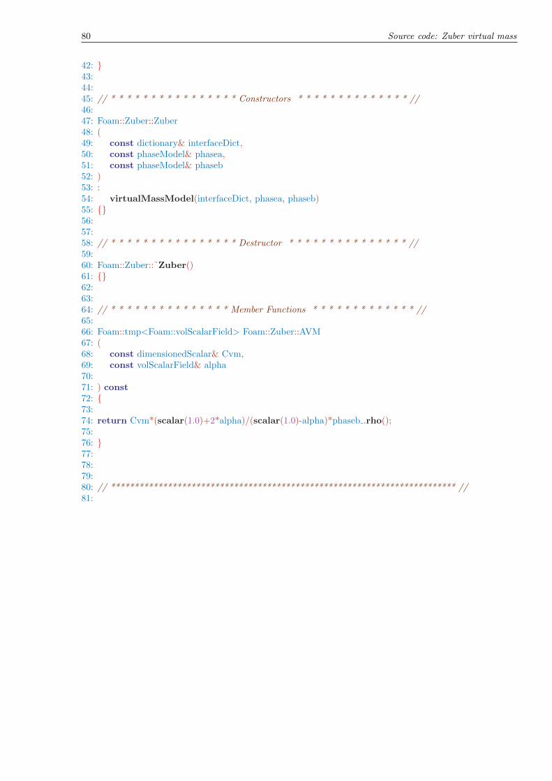
80 Source code: Zuber virtual mass
42: }43:44:45: // * * * * * * * * * * * * * * * * Constructors * * * * * * * * * * * * * * //46:47: Foam::Zuber::Zuber48: (49: const dictionary& interfaceDict,50: const phaseModel& phasea,51: const phaseModel& phaseb52: )53: :54: virtualMassModel(interfaceDict, phasea, phaseb)55: {}56:57:58: // * * * * * * * * * * * * * * * * Destructor * * * * * * * * * * * * * * * //59:60: Foam::Zuber::˜Zuber()61: {}62:63:64: // * * * * * * * * * * * * * * * Member Functions * * * * * * * * * * * * * //65:66: Foam::tmp<Foam::volScalarField> Foam::Zuber::AVM67: (68: const dimensionedScalar& Cvm,69: const volScalarField& alpha70:71: ) const72: {73:74: return Cvm*(scalar(1.0)+2*alpha)/(scalar(1.0)-alpha)*phaseb .rho();75:76: }77:78:79:80: // ************************************************************************* //81:

APPENDIXH
SOURCE CODE: HIBIKI-ISHII COALESCENCE MODEL
001: /*--–-–-–-–-–-–-–-–-–-–-–-–-–-–-–-–-–-–-–-–-–-–-–-–--*\002: ========= |003: \\ / F ield | OpenFOAM: The Open Source CFD Toolbox004: \\ / O peration |005: \\ / A nd | Copyright (C) 1991-2007 OpenCFD Ltd.006: \\/ M anipulation |007: --–-–-–-–-–-–-–-–-–-–-–-–-–-–-–-–-–-–-–-–-–-–-–-–-–-–008: License009: This file is part of OpenFOAM.010:011: OpenFOAM is free software; you can redistribute it and/or modify it012: under the terms of the GNU General Public License as published by the013: Free Software Foundation; either version 2 of the License, or (at your014: option) any later version.015:016: OpenFOAM is distributed in the hope that it will be useful, but WITHOUT017: ANY WARRANTY; without even the implied warranty of MERCHANTABILITY or018: FITNESS FOR A PARTICULAR PURPOSE. See the GNU General Public License019: for more details.020:021: You should have received a copy of the GNU General Public License022: along with OpenFOAM; if not, write to the Free Software Foundation,023: Inc., 59 Temple Place, Suite 330, Boston, MA 02111-1307 USA024:025: \*--–-–-–-–-–-–-–-–-–-–-–-–-–-–-–-–-–-–-–-–-–-–-–-–--*/026:027: #include ”HibikiIshiiC.H”028: #include ”addToRunTimeSelectionTable.H”029:030: // * * * * * * * * * * * * * * Static Data Members * * * * * * * * * * * * * //031:032: namespace Foam033: {034: defineTypeNameAndDebug(HibikiIshiiC, 0);035:036: addToRunTimeSelectionTable037: (038: coalescenceModel,039: HibikiIshiiC,040: dictionary041: );
81
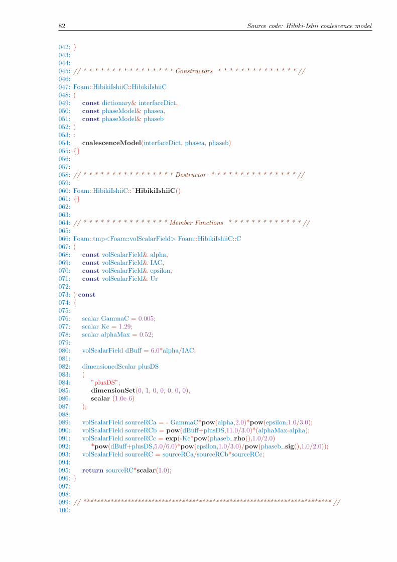
82 Source code: Hibiki-Ishii coalescence model
042: }043:044:045: // * * * * * * * * * * * * * * * * Constructors * * * * * * * * * * * * * * //046:047: Foam::HibikiIshiiC::HibikiIshiiC048: (049: const dictionary& interfaceDict,050: const phaseModel& phasea,051: const phaseModel& phaseb052: )053: :054: coalescenceModel(interfaceDict, phasea, phaseb)055: {}056:057:058: // * * * * * * * * * * * * * * * * Destructor * * * * * * * * * * * * * * * //059:060: Foam::HibikiIshiiC::˜HibikiIshiiC()061: {}062:063:064: // * * * * * * * * * * * * * * * Member Functions * * * * * * * * * * * * * //065:066: Foam::tmp<Foam::volScalarField> Foam::HibikiIshiiC::C067: (068: const volScalarField& alpha,069: const volScalarField& IAC,070: const volScalarField& epsilon,071: const volScalarField& Ur072:073: ) const074: {075:076: scalar GammaC = 0.005;077: scalar Kc = 1.29;078: scalar alphaMax = 0.52;079:080: volScalarField dBuff = 6.0*alpha/IAC;081:082: dimensionedScalar plusDS083: (084: ”plusDS”,085: dimensionSet(0, 1, 0, 0, 0, 0, 0),086: scalar (1.0e-6)087: );088:089: volScalarField sourceRCa = - GammaC*pow(alpha,2.0)*pow(epsilon,1.0/3.0);090: volScalarField sourceRCb = pow(dBuff+plusDS,11.0/3.0)*(alphaMax-alpha);091: volScalarField sourceRCc = exp(-Kc*pow(phaseb .rho(),1.0/2.0)092: *pow(dBuff+plusDS,5.0/6.0)*pow(epsilon,1.0/3.0)/pow(phaseb .sig(),1.0/2.0));093: volScalarField sourceRC = sourceRCa/sourceRCb*sourceRCc;094:095: return sourceRC*scalar(1.0);096: }097:098:099: // ************************************************************************* //100:

APPENDIX I
SOURCE CODE: HIBIKI-ISHII BREAKUP MODEL
001: /*--–-–-–-–-–-–-–-–-–-–-–-–-–-–-–-–-–-–-–-–-–-–-–-–--*\002: ========= |003: \\ / F ield | OpenFOAM: The Open Source CFD Toolbox004: \\ / O peration |005: \\ / A nd | Copyright (C) 1991-2007 OpenCFD Ltd.006: \\/ M anipulation |007: --–-–-–-–-–-–-–-–-–-–-–-–-–-–-–-–-–-–-–-–-–-–-–-–-–-–008: License009: This file is part of OpenFOAM.010:011: OpenFOAM is free software; you can redistribute it and/or modify it012: under the terms of the GNU General Public License as published by the013: Free Software Foundation; either version 2 of the License, or (at your014: option) any later version.015:016: OpenFOAM is distributed in the hope that it will be useful, but WITHOUT017: ANY WARRANTY; without even the implied warranty of MERCHANTABILITY or018: FITNESS FOR A PARTICULAR PURPOSE. See the GNU General Public License019: for more details.020:021: You should have received a copy of the GNU General Public License022: along with OpenFOAM; if not, write to the Free Software Foundation,023: Inc., 59 Temple Place, Suite 330, Boston, MA 02111-1307 USA024:025: \*--–-–-–-–-–-–-–-–-–-–-–-–-–-–-–-–-–-–-–-–-–-–-–-–--*/026:027: #include ”HibikiIshii.H”028: #include ”addToRunTimeSelectionTable.H”029:030: // * * * * * * * * * * * * * * Static Data Members * * * * * * * * * * * * * //031:032: namespace Foam033: {034: defineTypeNameAndDebug(HibikiIshii, 0);035:036: addToRunTimeSelectionTable037: (038: breakupModel,039: HibikiIshii,040: dictionary041: );
83

84 Source code: Hibiki-Ishii breakup model
042: }043:044:045: // * * * * * * * * * * * * * * * * Constructors * * * * * * * * * * * * * * //046:047: Foam::HibikiIshii::HibikiIshii048: (049: const dictionary& interfaceDict,050: const phaseModel& phasea,051: const phaseModel& phaseb052: )053: :054: breakupModel(interfaceDict, phasea, phaseb)055: {}056:057:058: // * * * * * * * * * * * * * * * * Destructor * * * * * * * * * * * * * * * //059:060: Foam::HibikiIshii::˜HibikiIshii()061: {}062:063:064: // * * * * * * * * * * * * * * * Member Functions * * * * * * * * * * * * * //065:066: Foam::tmp<Foam::volScalarField> Foam::HibikiIshii::B067: (068: const volScalarField& alpha,069: const volScalarField& IAC,070: const volScalarField& epsilon,071: const volScalarField& Ur072:073: ) const074: {075:076: scalar GammaB = 0.005;077: scalar Kb = 1.37;078: scalar alphaMax = 0.52;079:080: volScalarField dBuff = 6.0*alpha/IAC;081:082: dimensionedScalar plusDS083: (084: ”plusDS”,085: dimensionSet(0, 1, 0, 0, 0, 0, 0),086: scalar (1.0e-6)087: );088:089: volScalarField sourceTIa = GammaB*alpha*(1.0-alpha)*pow(epsilon,1.0/3.0);090: volScalarField sourceTIb = pow(dBuff+plusDS,11.0/3.0)*(alphaMax-alpha);091: volScalarField sourceTIc = exp(-Kb*phaseb .sig()/phaseb .rho()092: /pow(dBuff+plusDS,5.0/3.0)/pow(epsilon,2.0/3.0));093: volScalarField sourceTI = sourceTIa/sourceTIb*sourceTIc;094:095:096: return sourceTI*scalar(1.0);097: }098:099:100: // ************************************************************************* //101:

APPENDIX J
SOURCE CODE: YAO-MOREL COALESCENCE MODEL
001: /*--–-–-–-–-–-–-–-–-–-–-–-–-–-–-–-–-–-–-–-–-–-–-–-–--*\002: ========= |003: \\ / F ield | OpenFOAM: The Open Source CFD Toolbox004: \\ / O peration |005: \\ / A nd | Copyright (C) 1991-2007 OpenCFD Ltd.006: \\/ M anipulation |007: --–-–-–-–-–-–-–-–-–-–-–-–-–-–-–-–-–-–-–-–-–-–-–-–-–-–008: License009: This file is part of OpenFOAM.010:011: OpenFOAM is free software; you can redistribute it and/or modify it012: under the terms of the GNU General Public License as published by the013: Free Software Foundation; either version 2 of the License, or (at your014: option) any later version.015:016: OpenFOAM is distributed in the hope that it will be useful, but WITHOUT017: ANY WARRANTY; without even the implied warranty of MERCHANTABILITY or018: FITNESS FOR A PARTICULAR PURPOSE. See the GNU General Public License019: for more details.020:021: You should have received a copy of the GNU General Public License022: along with OpenFOAM; if not, write to the Free Software Foundation,023: Inc., 59 Temple Place, Suite 330, Boston, MA 02111-1307 USA024:025: \*--–-–-–-–-–-–-–-–-–-–-–-–-–-–-–-–-–-–-–-–-–-–-–-–--*/026:027: #include ”YaoMorelC.H”028: #include ”addToRunTimeSelectionTable.H”029:030: // * * * * * * * * * * * * * * Static Data Members * * * * * * * * * * * * * //031:032: namespace Foam033: {034: defineTypeNameAndDebug(YaoMorelC, 0);035:036: addToRunTimeSelectionTable037: (038: coalescenceModel,039: YaoMorelC,040: dictionary041: );
85
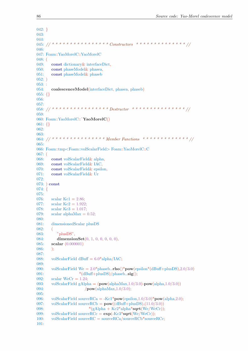
86 Source code: Yao-Morel coalescence model
042: }043:044:045: // * * * * * * * * * * * * * * * * Constructors * * * * * * * * * * * * * * //046:047: Foam::YaoMorelC::YaoMorelC048: (049: const dictionary& interfaceDict,050: const phaseModel& phasea,051: const phaseModel& phaseb052: )053: :054: coalescenceModel(interfaceDict, phasea, phaseb)055: {}056:057:058: // * * * * * * * * * * * * * * * * Destructor * * * * * * * * * * * * * * * //059:060: Foam::YaoMorelC::˜YaoMorelC()061: {}062:063:064: // * * * * * * * * * * * * * * * Member Functions * * * * * * * * * * * * * //065:066: Foam::tmp<Foam::volScalarField> Foam::YaoMorelC::C067: (068: const volScalarField& alpha,069: const volScalarField& IAC,070: const volScalarField& epsilon,071: const volScalarField& Ur072:073: ) const074: {075:076: scalar Kc1 = 2.86;077: scalar Kc2 = 1.922;078: scalar Kc3 = 1.017;079: scalar alphaMax = 0.52;080:081: dimensionedScalar plusDS082: (083: ”plusDS”,084: dimensionSet(0, 1, 0, 0, 0, 0, 0),085: scalar (0.000001)086: );087:088: volScalarField dBuff = 6.0*alpha/IAC;089:090: volScalarField We = 2.0*phaseb .rho()*pow(epsilon*(dBuff+plusDS),2.0/3.0)091: *(dBuff+plusDS)/phaseb .sig();092: scalar WeCr = 1.24;093: volScalarField gAlpha = (pow(alphaMax,1.0/3.0)-pow(alpha,1.0/3.0))094: /pow(alphaMax,1.0/3.0);095:096: volScalarField sourceRCa = -Kc1*pow(epsilon,1.0/3.0)*pow(alpha,2.0);097: volScalarField sourceRCb = pow((dBuff+plusDS),(11.0/3.0))098: *(gAlpha + Kc2*alpha*sqrt(We/WeCr));099: volScalarField sourceRCc = exp(-Kc3*sqrt(We/WeCr));100: volScalarField sourceRC = sourceRCa/sourceRCb*sourceRCc;101:

87
102: return sourceRC*scalar(1.0);103: }104:105:106: // ************************************************************************* //107:

88 Source code: Yao-Morel coalescence model
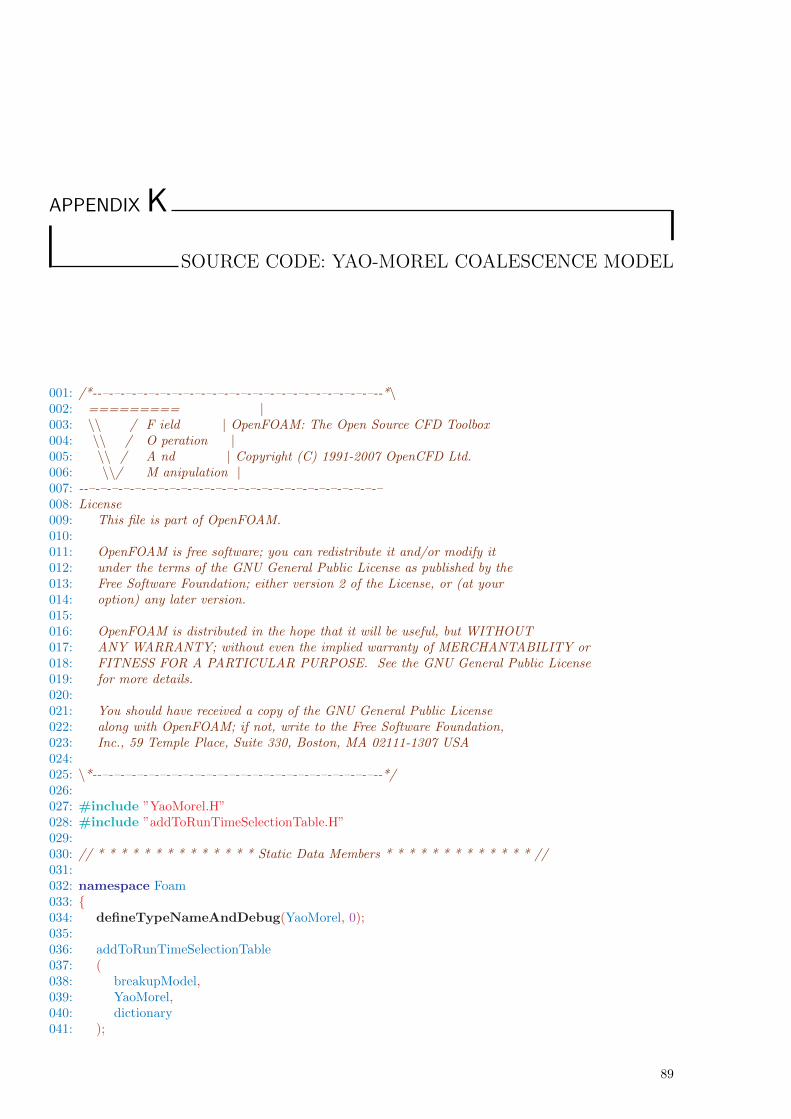
APPENDIXK
SOURCE CODE: YAO-MOREL COALESCENCE MODEL
001: /*--–-–-–-–-–-–-–-–-–-–-–-–-–-–-–-–-–-–-–-–-–-–-–-–--*\002: ========= |003: \\ / F ield | OpenFOAM: The Open Source CFD Toolbox004: \\ / O peration |005: \\ / A nd | Copyright (C) 1991-2007 OpenCFD Ltd.006: \\/ M anipulation |007: --–-–-–-–-–-–-–-–-–-–-–-–-–-–-–-–-–-–-–-–-–-–-–-–-–-–008: License009: This file is part of OpenFOAM.010:011: OpenFOAM is free software; you can redistribute it and/or modify it012: under the terms of the GNU General Public License as published by the013: Free Software Foundation; either version 2 of the License, or (at your014: option) any later version.015:016: OpenFOAM is distributed in the hope that it will be useful, but WITHOUT017: ANY WARRANTY; without even the implied warranty of MERCHANTABILITY or018: FITNESS FOR A PARTICULAR PURPOSE. See the GNU General Public License019: for more details.020:021: You should have received a copy of the GNU General Public License022: along with OpenFOAM; if not, write to the Free Software Foundation,023: Inc., 59 Temple Place, Suite 330, Boston, MA 02111-1307 USA024:025: \*--–-–-–-–-–-–-–-–-–-–-–-–-–-–-–-–-–-–-–-–-–-–-–-–--*/026:027: #include ”YaoMorel.H”028: #include ”addToRunTimeSelectionTable.H”029:030: // * * * * * * * * * * * * * * Static Data Members * * * * * * * * * * * * * //031:032: namespace Foam033: {034: defineTypeNameAndDebug(YaoMorel, 0);035:036: addToRunTimeSelectionTable037: (038: breakupModel,039: YaoMorel,040: dictionary041: );
89

90 Source code: Yao-Morel coalescence model
042: }043:044:045: // * * * * * * * * * * * * * * * * Constructors * * * * * * * * * * * * * * //046:047: Foam::YaoMorel::YaoMorel048: (049: const dictionary& interfaceDict,050: const phaseModel& phasea,051: const phaseModel& phaseb052: )053: :054: breakupModel(interfaceDict, phasea, phaseb)055: {}056:057:058: // * * * * * * * * * * * * * * * * Destructor * * * * * * * * * * * * * * * //059:060: Foam::YaoMorel::˜YaoMorel()061: {}062:063:064: // * * * * * * * * * * * * * * * Member Functions * * * * * * * * * * * * * //065:066: Foam::tmp<Foam::volScalarField> Foam::YaoMorel::B067: (068: const volScalarField& alpha,069: const volScalarField& IAC,070: const volScalarField& epsilon,071: const volScalarField& Ur072:073: ) const074: {075:076: scalar Kb1 = 1.6;077: scalar Kb2 = 0.42;078: scalar alphaMax = 0.52;079:080: dimensionedScalar plusDS081: (082: ”plusDS”,083: dimensionSet(0, 1, 0, 0, 0, 0, 0),084: scalar (0.000001)085: );086:087: volScalarField dBuff = 6.0*alpha/IAC;088:089: volScalarField We = 2.0*phaseb .rho()*pow(epsilon*(dBuff+plusDS),2.0/3.0)090: *(dBuff+plusDS)/phaseb .sig();091: scalar WeCr = 1.24;092:093: volScalarField gAlpha = (pow(alphaMax,1.0/3.0)-pow(alpha,1.0/3.0))094: /pow(alphaMax,1.0/3.0);095:096: volScalarField sourceTIa = Kb1*pow(epsilon,1.0/3.0)*alpha*(1.0-alpha);097: volScalarField sourceTIb = pow((dBuff+plusDS),(11.0/3.0))*(1.0+Kb2*(1.0-alpha)098: *sqrt(We/WeCr));099: volScalarField sourceTIc = exp(-WeCr/We);100: volScalarField sourceTI = sourceTIa/sourceTIb*sourceTIc;101:
91
102: return sourceTI*scalar(1.0);103: }104:105:106: // ************************************************************************* //107:

92 Source code: Yao-Morel coalescence model
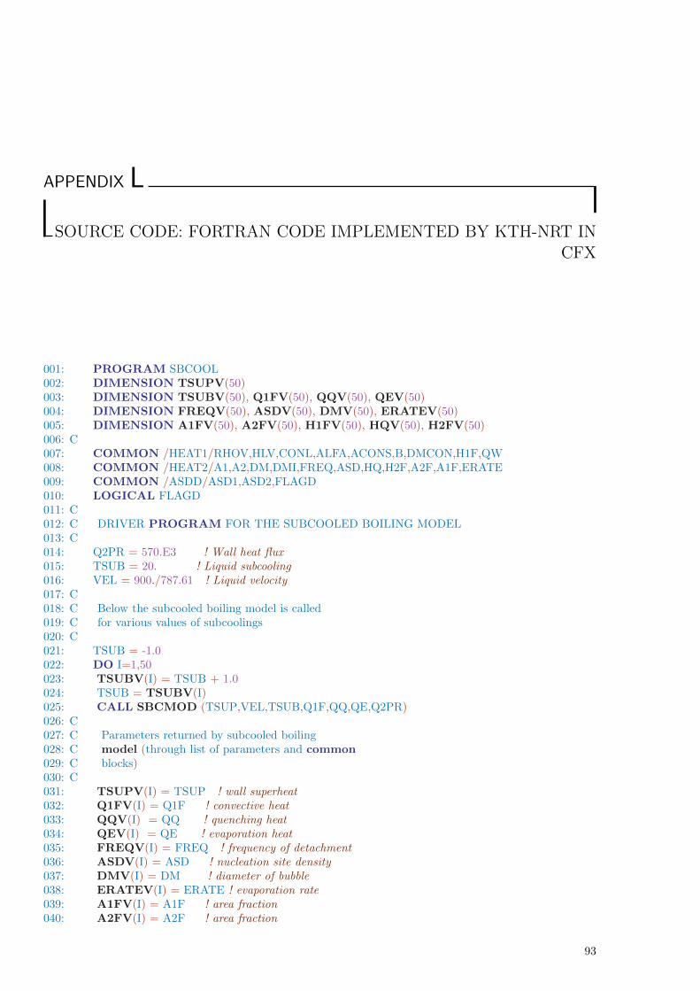
APPENDIX L
SOURCE CODE: FORTRAN CODE IMPLEMENTED BY KTH-NRT INCFX
001: PROGRAM SBCOOL002: DIMENSION TSUPV(50)003: DIMENSION TSUBV(50), Q1FV(50), QQV(50), QEV(50)004: DIMENSION FREQV(50), ASDV(50), DMV(50), ERATEV(50)005: DIMENSION A1FV(50), A2FV(50), H1FV(50), HQV(50), H2FV(50)006: C007: COMMON /HEAT1/RHOV,HLV,CONL,ALFA,ACONS,B,DMCON,H1F,QW008: COMMON /HEAT2/A1,A2,DM,DMI,FREQ,ASD,HQ,H2F,A2F,A1F,ERATE009: COMMON /ASDD/ASD1,ASD2,FLAGD010: LOGICAL FLAGD011: C012: C DRIVER PROGRAM FOR THE SUBCOOLED BOILING MODEL013: C014: Q2PR = 570.E3 ! Wall heat flux015: TSUB = 20. ! Liquid subcooling016: VEL = 900./787.61 ! Liquid velocity017: C018: C Below the subcooled boiling model is called019: C for various values of subcoolings020: C021: TSUB = -1.0022: DO I=1,50023: TSUBV(I) = TSUB + 1.0024: TSUB = TSUBV(I)025: CALL SBCMOD (TSUP,VEL,TSUB,Q1F,QQ,QE,Q2PR)026: C027: C Parameters returned by subcooled boiling028: C model (through list of parameters and common029: C blocks)030: C031: TSUPV(I) = TSUP ! wall superheat032: Q1FV(I) = Q1F ! convective heat033: QQV(I) = QQ ! quenching heat034: QEV(I) = QE ! evaporation heat035: FREQV(I) = FREQ ! frequency of detachment036: ASDV(I) = ASD ! nucleation site density037: DMV(I) = DM ! diameter of bubble038: ERATEV(I) = ERATE ! evaporation rate039: A1FV(I) = A1F ! area fraction040: A2FV(I) = A2F ! area fraction
93
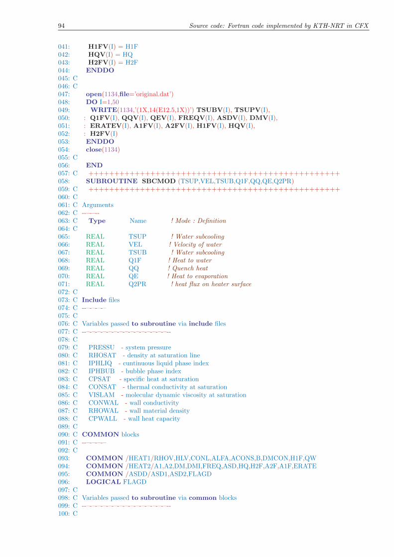
94 Source code: Fortran code implemented by KTH-NRT in CFX
041: H1FV(I) = H1F042: HQV(I) = HQ043: H2FV(I) = H2F044: ENDDO045: C046: C047: open(1134,file=’original.dat’)048: DO I=1,50049: WRITE(1134,’(1X,14(E12.5,1X))’) TSUBV(I), TSUPV(I),050: : Q1FV(I), QQV(I), QEV(I), FREQV(I), ASDV(I), DMV(I),051: : ERATEV(I), A1FV(I), A2FV(I), H1FV(I), HQV(I),052: : H2FV(I)053: ENDDO054: close(1134)055: C056: END057: C +++++++++++++++++++++++++++++++++++++++++++++++++058: SUBROUTINE SBCMOD (TSUP,VEL,TSUB,Q1F,QQ,QE,Q2PR)059: C +++++++++++++++++++++++++++++++++++++++++++++++++060: C061: C Arguments062: C --–-–--063: C Type Name ! Mode : Definition064: C065: REAL TSUP ! Water subcooling066: REAL VEL ! Velocity of water067: REAL TSUB ! Water subcooling068: REAL Q1F ! Heat to water069: REAL QQ ! Quench heat070: REAL QE ! Heat to evaporation071: REAL Q2PR ! heat flux on heater surface072: C073: C Include files074: C --–-–-–-–075: C076: C Variables passed to subroutine via include files077: C --–-–-–-–-–-–-–-–-–-–-–-–-–-–-–--078: C079: C PRESSU - system pressure080: C RHOSAT - density at saturation line081: C IPHLIQ - cuntinuous liquid phase index082: C IPHBUB - bubble phase index083: C CPSAT - specific heat at saturation084: C CONSAT - thermal conductivity at saturation085: C VISLAM - molecular dynamic viscosity at saturation086: C CONWAL - wall conductivity087: C RHOWAL - wall material density088: C CPWALL - wall heat capacity089: C090: C COMMON blocks091: C --–-–-–-–092: C093: COMMON /HEAT1/RHOV,HLV,CONL,ALFA,ACONS,B,DMCON,H1F,QW094: COMMON /HEAT2/A1,A2,DM,DMI,FREQ,ASD,HQ,H2F,A2F,A1F,ERATE095: COMMON /ASDD/ASD1,ASD2,FLAGD096: LOGICAL FLAGD097: C098: C Variables passed to subroutine via common blocks099: C --–-–-–-–-–-–-–-–-–-–-–-–-–-–-–--100: C

95
101: C102: C Locals103: C --–--104: C Type Name ! Definition105: C106: C Set initial values for locals107: C --–-–-–-–-–-–-–-–-–-108: C109: C Save locals110: C --–-–-–-–111: C SBCMOD--–-–-–-–-–-–-–-–-–-–-–-–-–-–-–-–-END-OF-HEADING112: C113: C INITIALIZE114: C115: A1 = 0.E0116: A2 = 0.E0117: DM = 0.E0118: DMI = 0.E0119: FREQ = 0.E0120: ASD = 0.E0121: HQ = 0.E0122: H2F = 0.E0123: A2F = 0.E0124: A1F = 0.E0125: ERATE= 0.E0126: TW = 0.E0127: Q1F = 0.E0128: QQ = 0.E0129: QE = 0.E0130: QW = Q2PR131: C132: C ==========================================================133: C PROPERTIES AT P=45 BAR134: PRES = 45.e5135: RHOL = 787.61136: RHOV = 22.70137: CPL = 4949.18138: CONL = 0.6088139: VISK = 1.305127e-7140: CONW = 19.0141: RHOW = 7865.0142: CPW = 400.0143: SIGMA = 0.02429144: HFG = 1675854.0145: C CALCULATED PROPERTIES146: VISD = VISK*RHOL147: PRL = VISD*CPL/CONL148: ALFA = CONL/RHOL/CPL149: C150: HLV = HFG + CPL*TSUB151: C152: C ==========================================================153: C154: GAMA = SQRT(CONW*RHOW*CPW/CONL/RHOL/CPL)155: A1 = SQRT((RHOL-RHOV)*9.81E0/SIGMA)/(HFG*VISD)156: A2 = 0.5E0*SQRT(ALFA/3.14159E0)*0.013E0*PRL**1.7E0*GAMA157: C158: BCONS = 1.E0/2.E0/(1.E0-RHOV/RHOL)159: DMCON = 2.42E-5*PRES**0.709E0160: C
96 Source code: Fortran code implemented by KTH-NRT in CFX
161: C ==========================================================162: C163: C delta = 0.0001925164: C165: REYNO = VEL*3.2586E-4/VISK166: C167: CF = 0.062E0168: DO I = 1,10169: CF = 1.E0/( ALOG(REYNO*CF)/0.435E0 + 5.05E0 )170: END DO171: C172: C CF = sqrt (actual Cf/2)173: C Ch = s/(1+12.8(Prˆ0.68 - 1) sqrt(s))174: C175: H1F = CF*CF/(1.E0- 1.783E0*CF)176: H1F = H1F*RHOL*CPL*VEL177: C178: C ==============================================================179: C GUESS TSUP180: TSUP = QW/H1F-TSUB181: C IS IT ALREADY IN SINGLE PHASE ?182: FLAGD = .FALSE.183: IF (TSUP.LE.0.05E0) THEN184: DM = 0.E0185: ASD = 0.E0186: FREQ = 0.E0187: HQ = 0.E0188: A1F = 1.E0189: GO TO 130190: END IF191: C192: IF (TSUB.GT.2.E0) THEN193: B = TSUB*BCONS194: ELSE195: TMAX = QW/H1F-0.001E0196: IF (TMAX.GT.3) TMAX = 3.E0197: IF (TMAX.LT.2) THEN198: FLAGD = .TRUE.199: WRITE (*,*) ’ SWITCHED TO TOLUBINSKY DIAM.’200: GO TO 25201: END IF202: C203: B2 = 2.E0*BCONS204: B3 = TMAX*BCONS205: C206: AA2 = (A1*(QW - H1F*2.E0))**0.33333E0*A2207: AA3 = (A1*(QW - H1F*TMAX))**0.33333E0*A2208: IF (VEL.LT.0.61E0) FI=1.E0209: IF (VEL.GE.0.61E0) FI=(VEL/0.61E0)**0.47E0210: DM2 = DMCON*AA2/SQRT(B2*FI)211: DM3 = DMCON*AA3/SQRT(B3*FI)212: DMI = DM2 + (DM3-DM2)*(TSUB-2.E0)/(TMAX-2.E0)213: C214: END IF215: 25 CONTINUE216: C --–-–-–-–-–-–-–-–-–-–-–-–-–-–-– START ITERATION217: C218: ITLIM=100219: RELAX =0.5E0220: 110 ITER =0

97
221: 120 ITER = ITER+1222: IF (ITER.GT.ITLIM) THEN223: ITLIM=ITLIM+50224: RELAX=0.6E0*RELAX225: IF (RELAX.LT.0.005E0) THEN226: WRITE (*,*) ’TSUB = ’,TSUB,’ VEL = ’,VEL227: WRITE (*,*) ’COULD NOT FIND WALL TEMP.’228: TSUP = -TSUB229: RETURN230: END IF231: GO TO 120232: END IF233: C234: CALL SBHEAT(TSUP,TSUB,VEL)235: HH = A1F*H1F + A2F*HQ236: QTOT = ERATE*HLV + HH*(TSUB+TSUP)237: IF (HH.EQ.0.E0) THEN238: TSUP1 = -TSUB239: ELSE240: TSUP1 = TSUP + RELAX*(QW-QTOT)/HH241: IF (TSUP1.LE.-TSUB) TSUP1=-TSUB242: END IF243: C244: ERR = ABS((QTOT-QW)/QW)245: IF (TSUP1.LE.0.E0) TSUP1 = 0.8E0*TSUP246: TSUP = TSUP1247: IF (ERR.GT.1.E-5) GO TO 120248: C249: 130 CONTINUE250: C251: Q1F = A1F*H1F*(TSUP+TSUB)252: QQ = A2F*HQ*(TSUP+TSUB)253: QE = ERATE*HLV254: C255: RETURN256: END257: C ++++++++++++++++++++++++++++++++++++258: SUBROUTINE SBHEAT (TSUP, TSUB, VEL)259: C ++++++++++++++++++++++++++++++++++++260: C261: C Arguments262: C --–-–--263: C Type Name ! Mode : Definition264: C265: REAL TSUP ! Wall superheat (Twall-Tsat)266: REAL TSUB ! Water subcooling (Tsat-Tliq)267: REAL VEL ! Water velocity268: C269: C Include files270: C --–-–-–-–271: C272: C COMMON blocks273: C --–-–-–-–274: C275: COMMON /HEAT1/RHOV,HLV,CONL,ALFA,ACONS,B,DMCON,H1F,QW276: COMMON /HEAT2/A1,A2,DM,DMI,FREQ,ASD,HQ,H2F,A2F,A1F,ERATE277: COMMON /ASDD/ASD1,ASD2,FLAGD278: LOGICAL FLAGD279: C280: C Variables passed to subroutine via common blocks
98 Source code: Fortran code implemented by KTH-NRT in CFX
281: C --–-–-–-–-–-–-–-–-–-–-–-–-–-–-–--282: C283: C SBHEAT--–-–-–-–-–-–-–-–-–-–-–-–-–-–-–-–-END-OF-HEADING284: C285: ASD = 0.0286: C287: IF (TSUB.GT.2.E0) THEN288: A = (A1*(QW - H1F*TSUB))**0.33333E0*A2289: IF (VEL.LT.0.61E0) FI=1.E0290: IF (VEL.GE.0.61E0) FI=(VEL/0.61E0)**0.47E0291: DM = DMCON*A/SQRT(B*FI)292: ELSE293: IF (FLAGD) THEN294: DM = 0.0014E0*EXP(-TSUB/45.E0)295: ELSE296: DM = DMI297: END IF298: END IF299: FREQ = 3.546E0/SQRT(DM)300: IF (TSUP.LE.0.0001E0) TSUP=0.0001E0301: ASD = (210.E0*TSUP)**1.805E0302: C write(*,*) ’DM,FREQ,ASD=’,DM,FREQ,ASD303: C304: C305: ATOT = 1.E0306: A2F = 3.1415E0*DM*DM*ASD307: A1F = ATOT - A2F308: C309: IF (A1F.LE.1.E-4) THEN310: A2F = ATOT311: A1F = 1.E-4312: ASD = 1.E0/3.1415E0/DM/DM313: END IF314: C315: ERATE = 3.14159E0*DM*DM*DM/6.E0*ASD*FREQ*RHOV316: EMAX = QW/HLV317: IF (ERATE.GT.EMAX) ERATE = EMAX318: C319: HQ = 2.E0*CONL/SQRT(3.14159E0*ALFA/FREQ)320: C321: RETURN322: END323: