General rights Copyright and moral rights for the publications made accessible in the public portal are retained by the authors and/or other copyright owners and it is a condition of accessing publications that users recognise and abide by the legal requirements associated with these rights.

Users may download and print one copy of any publication from the public portal for the purpose of private study or research.

You may not further distribute the material or use it for any profit-making activity or commercial gain

You may freely distribute the URL identifying the publication in the public portal If you believe that this document breaches copyright please contact us providing details, and we will remove access to the work immediately and investigate your claim.

Downloaded from orbit.dtu.dk on: Apr 20, 2020

Modeling of Salinity Effects on Waterflooding of Petroleum Reservoirs

Alexeev, Artem

Publication date:2015

Document VersionPeer reviewed version

Link back to DTU Orbit

Citation (APA):Alexeev, A. (2015). Modeling of Salinity Effects on Waterflooding of Petroleum Reservoirs. Kgs. Lyngby:Technical University of Denmark.

Artem Alexeev Ph.D. Thesis December 2015

Modeling of Salinity Effects on Water-flooding of Petroleum Reservoirs

Center for Energy Resources Engineering

Department of Chemical and

Biochemical Engineering

Technical University of Denmark

Søltofts Plads, Building 229

DK-2800 Kgs. Lyngby

Tlf. +45 4525 2800

Fax +45 4525 4588

www.cere.dtu.dk

Modeling of Salinity Effects on W

aterflooding of Petroleum Reservoirs

Artem

Alexeev

Modeling of Salinity Effects on Waterflooding of Petroleum Reservoirs

Modeling of Salinity Effects on

Waterflooding of Petroleum Reservoirs

Artem Alexeev

PhD Thesis

December 2015

Center for Energy Resources Engineering

Department of Chemical and Biochemical Engineering

Technical University of Denmark

Kongens Lyngby, Denmark

Technical University of Denmark

Department of Chemical and Biochemical Engineering

Building 229, DK-2800 Kongens Lyngby, Denmark

Phone: +45 4525 2800

Fax: +45 4525 4588

Web: www.cere.dtu.dk

Copyright © Artem Alexeev, 2016

Printed by GraphicCo A/S, Denmark

Preface

This thesis is submitted as partial fulfillment of the requirement for the Ph.D. degree at

Technical University of Denmark (DTU). The work has been carried out at the Department

of Chemical and Biochemical Engineering and Center for Energy Resources Engineering

(CERE) from September 2012 to November 2015 under the supervision of Associate

Professor Alexander Shapiro as the main supervisor and Associate Professor Kaj Thomsen

as the co-supervisor. The project was supported by DONG Energy, Mærsk Oil, and the

Danish EUDP program (a program for development and demonstration of energy

technology) under the Danish Energy Agency, and by the Danish research councils.

First and foremost, I wish to express my deepest gratitude to Alexander Shapiro for his

guidance on my research. I admire your profound knowledge in many different fields of

science and beyond which you have been sharing with me during our numerous discussions.

Your encouragement, patience, and support were extremely valuable to me. I am also grateful

to Kaj Thomsen and all members of the SmartWater project for collaboration, useful

discussions, and suggestions.

During the course of the study, I had a chance to spend 3 month at the Australian School of

Petroleum (ASP), University of Adelaide, South Australia. Special thanks to Professor Pavel

Bedrikovetsky for kindly hosting my visit and making me feel a part of ASP. Thanks to my

friends at ASP, and especially Sara Borazjani for the interesting collaboration.

I would especially like to acknowledge my friend and colleague Tina Katika, who provided

me with a lot of help and support. Thank you for our chitchats during coffee breaks at DTU

and numerous profound scientific discussions held in Copenhagen bars.

I am also grateful to my dear colleagues at CERE for providing a comfortable and stimulating

research environment.

Kongens Lyngby, December 2015

Artem Alexeev

iv

Summary

Smart Water flooding is an enhanced oil recovery (EOR) technique that is based on the

injection of chemistry-optimized water with changed ionic composition and salinity into

petroleum reservoirs. Extensive research that has been carried out over the past two decades

has clearly demonstrated that smart water flooding can improve the ultimate oil recovery

both in carbonate and sandstone reservoirs. A number of different physicochemical

mechanisms of action were proposed to explain the smart water effects, but none of them has

commonly been accepted as a determining mechanism.

Most of the experimental studies concerning the smart water effects recognize importance of

the chemistry of reservoir rocks that manifests itself in dissolution and precipitation of rock

minerals and adsorption of specific ions on the rock surface. The brine-rock interactions may

affect the wetting state of the rock and in some cases result in mobilization of the trapped oil.

In this thesis, we set up a generic model for the reactive transport in porous media to

investigate how different mechanisms influence the oil recovery, pressure distribution and

composition of the brine during forced displacement. We consider several phenomena related

to the smart water effects, such as mineral dissolution, adsorption of potential determining

ions in carbonate rocks, and mechanisms that influence mobilization of the trapped oil and

its transport.

Dissolution of minerals occurs due to the different compositions of the injected brine and the

formation water that is initially in equilibrium with the reservoir rock. We consider a

displacement process in one dimension with dissolution affecting both the

porosity/permeability of the rock and the density of the brine. Extending previous studies, we

account for the different individual volumes of mineral in solid and in solution, which is

found to affect slightly the velocity of the displacement front.

The rate of dissolution is found to have a significant influence on the evolution of the rock

properties. At low reaction rates, dissolution occurs across the entire region between the

injection and production sites resulting in heterogeneous porosity and permeability fields.

Fast dissolution resembles formation of wormholes with a significant change in porosity and

permeability close to the injection site.

Further, we study the mechanisms that can govern the mobilization of residual oil and its

flow in porous media. The oil trapped in the swept zones after conventional flooding is

present in a form of disconnected oil drops, or oil ganglia. While the macroscopic theory of

multiphase flow assumes that fluid phases flow in their own pore networks and do not

vi Summary

influence each other, the flow of disconnected oil ganglia requires an alternative description.

We address this problem by considering a micromodel for the two-phase flow in a single

angular pore-body.

On the micro-level, both fluids can be present in a single pore body and interact during the

flow. Considering water-wet systems, we find that presence of the water on the surface of the

rock and in the corner filaments of pore bodies results in a larger velocity of the viscous flow

of the oil phase due to the increased area of the moving oil-water interface. Moreover, the

flow of oil may be induced solely by the action of viscous forces at the oil-water interface,

which appears to be a new mechanism for the transport of disconnected oil ganglia in porous

media. We derive correlations that allow calculating the flow velocities of fluid phases in

single pore bodies based on the pore fluid saturations.

Based on the microscale considerations, we develop a macroscopic model of displacement

accounting for the effects associated with oil ganglia. The model is based on the assumption

that wettability alteration toward increased water-wetness caused by the presence of active

species in the injected brine results in formation of the wetting films on the surface of the

rock. Oil ganglia are mobilized and carried by the slow flow of wetting films. Considering

simplistic pore-network model, we derive the macroscopic system of equations involving

description of the transport of oil ganglia. As a result of numerical modeling of the tertiary

recovery process, it is found that production of oil ganglia may continue for a long time of

injection of around 10 to 20 PVI.

Unlike the conventional models of chemical flooding, where mobilized oil bank travels ahead

of the concentration front, the oil ganglia model predicts that the mobilized oil is produced

after the active species reaches the effluent. Further extension of the model is achieved by

introduction of the non-equilibrium alteration of wettability and non-instantaneous oil

mobilization. Such modifications may explain the delay observed in some experiments,

where mobilized oil is produced during a long time after several pore volumes of injection.

One of the possible chemical mechanisms through which the mobilization of the residual oil

may occur in carbonates is alteration of the electrostatic potential of the surface. Reduction

of the surface charge due to adsorption of the potential determining ions results in the

decrease in oil affinity towards the surface of the rock. We establish a mathematical model

that takes into account adsorption of the potential determining ions: calcium, magnesium,

and sulfate, on the chalk surface, to investigate how the composition of the injected brine

affects the equilibrium surface composition and how adsorption process affects the

composition of the produced brine. We use experimental data on the produced brine

composition from the flow-through experiments to estimate the parameters of the adsorption

model. The computations suggest that there is no evidence of usually assumed stronger

adsorption of magnesium ion compared to calcium at high temperatures. In order to

investigate the effect of surface composition on the flooding efficiency, we combine the

adsorption model with the Buckley-Leverett model and perform simulations of the

experiments concerning flooding in the water-wet outcrop chalk. Computations of the

vii

equilibrium surface composition demonstrate a correlation between the concentration of the

adsorbed sulfate and the ultimate recovery observed in the experiments indicating that a more

negatively charged surface of chalk could be a factor that affects the recovery efficiency

without wettability modification.

viii Summary

Resume på dansk

”Smart water flooding” er en forbedret olieindvindings (EOR) teknik, der er baseret på

injektion af vand med kemisk optimeret saltindhold i olie reservoirer. Omfattende forskning,

der er udført i løbet af de seneste to årtier har tydeligt vist, at smart water flooding kan

forbedre den ultimative olieindvindingsgrad både i carbonat- og i sandstens- reservoirer. Der

er blevet foreslået en række forskellige fysisk-kemiske mekanismer til at forklare smart water

effekten, men ingen af dem har været almindeligt accepteret som den dominerende

mekanisme.

De fleste af de eksperimentelle undersøgelser vedrørende smart water effekter anerkender

betydningen af den kemiske interaktion mellem reservoir-klippe og den gennemstrømmende

saltopløsning, der manifesterer sig ved opløsning og udfældning af klippe-mineraler og

adsorption af specifikke ioner på klippens overflade. Interaktionen med saltopløsningen kan

påvirke klippens befugtningstilstand og i nogle tilfælde resultere i mobilisering af blokeret

olie.

I denne afhandling, opstiller vi en generel model for reaktiv transport i porøse medier for at

undersøge, hvordan forskellige mekanismer påvirker olieindvinding, trykfordeling og

sammensætning af saltopløsninger under tvungen gennemstrømning. Vi behandler flere

fænomener i relation til smart water effekten, såsom opløsning af mineraler, adsorption af

potentielt vigtige ioner i kalksten, og mekanismer, der har indflydelse på mobilisering af den

blokerede olie og transporten af denne.

Opløsning af mineraler finder sted på grund af de forskellige sammensætninger af den

injicerede saltopløsning og formationsvandet, der oprindeligt var i ligevægt med reservoiret.

Vi betragter en gennemstrømningsproces i en enkelt dimension hvor opløsning af mineralsk

materiale påvirker både porøsitet/permeabilitet af reservoiret og densiteten af

saltopløsningen. Vi videreudvikler tidligere undersøgelser ved at redegøre for de forskellige

individuelle mængder af mineral i fast form og i opløsning, som har vist sig at have en svag

effekt på hastigheden af gennemstrømningsfronten.

Hastigheden for mineralers opløsning viser sig at have en betydelig indflydelse på

udviklingen af reservoirets egenskaber. Ved lave reaktionshastigheder forekommer

opløsning i hele området mellem injektions- og produktionssteder og resulterer i heterogene

porøsitet og permeabilitet områder. Hurtig opløsning ligner dannelsen af ormehuller som

fører til en betydelig ændring i porøsitet og permeabilitet tæt på injektionsstedet.

x Resume på dansk

Endvidere studerer vi de mekanismer, der kan kontrollere mobiliseringen af resterende olie

og dens flow i porøse medier. Den olie der er tilbage i de bestrøgne zoner efter konventionelle

udvindinger er til stede i form af separate oliedråber eller olie ganglia. Den makroskopiske

teori om flerfasestrømning forudsætter, at fluide faser strømmer i deres egne pore netværk

uden at påvirke hinanden. Strømmen af sparate olie ganglia kræver en alternativ beskrivelse.

Vi løser dette problem ved at overveje en micromodel for tofaset strømning i et enkelvinklet

porevolumen.

På mikro-niveau, kan begge væsker være til stede i et enkelt pore volumen og interagere

mens væsken strømmer. For water-wet systemer, finder vi, at tilstedeværelsen af vand på

overfladen af reservoirmaterialet resulterer i en større hastighed i den viskøse strømning af

oliefasen på grund af det øgede grænsefladeareal mellem olie og vand. Desuden kan

oliestrømmen sættes i bevægelse udelukkende induceret af virkningen af viskøse kræfter ved

olie-vand-grænsefladen. Dette lader til at være en ny mekanisme til transport af olie afbrudt

ganglier i porøse medier. Vi udleder sammenhænge, som tillader beregning af

strømningshastigheder af væskefaser i individuelle porer baseret på mætningsgraden af

porens væske.

Baseret på de mikroskala betragtninger, udvikler vi en makroskopisk model for strømning i

porer, der indberegner de virkninger, der er forbundet med olie ganglia. Modellen er baseret

på den antagelse, at befugtningsændring mod øget water-wetness forårsaget af

tilstedeværelsen af aktive ioner i det injicerede saltvand resulterer i dannelse af en fugt-film

på overfladen af reservoirmaterialet. Olie ganglia mobiliseres og føres frem af den

langsomme strøm af fugt-film. I betragtning af denne simplistiske pore-netværksmodel,

udleder vi det makroskopiske ligningsystem, der involverer beskrivelse af transport af olie

ganglia. Som et resultat af numerisk modellering af den tertiære indvindingsproces, er det

konstateret, at produktionen af olie ganglia kan fortsætte i lang tid under injektionen, op til

10 til 20 PVI.

I modsætning til de traditionelle modeller for kemiske udskylninger, hvor en mobiliseret olie

front bevæger foran koncentrationfronten, forudsiger olie ganglia modellen at den

mobiliserede olie produceres efter de aktive ioner når frem. Yderligere udvidelse af modellen

er opnået ved indføring af non-equilibrium ændring af befugtning og forsinket olie

mobilisering. Sådanne modifikationer kan forklare forsinkelsen observeret i nogle

eksperimenter, hvor mobiliseret olie produceres i lang tid efter flere porevolumener er

injiceret.

En af de mulige kemiske mekanismer der mobiliserer resterende olie i kalk reservoirer er

ændring af det elektrostatiske potentiale af overfladen. Reduktion af overfladeladningen som

følge af adsorption af de potential bestemmende ioner resulterer i et fald i oliens affinitet for

reservoiroverfladen. Vi etablere en matematisk model, der tager højde for adsorption af

potential bestemmelse ioner: calcium, magnesium og sulfat på kalk overflader for at

undersøge, hvordan sammensætningen af den injicerede saltopløsning påvirker ligevægten

med overfladen, og hvordan adsorptionsprocessens påvirker sammensætningen af det

xi

producerede saltvand. Vi bruger eksperimentelle data målt på saltvand produceret ved

gennemstrømning af reservoirkerne. Beregningerne tyder på, at der ikke er tegn på en

stærkere adsorption af magnesium ion sammenlignet med calcium ion ved høje temperaturer,

som det ellers ofte antages.

For at undersøge overfladesammensætningens effekt på gennemstrømningens effektivitet,

kombinerer vi adsorption modellen med Buckley-Leverett modellen og udfører simuleringer

af forsøgene vedrørende gennemstrømninger i water-wet outcrop kridt. Beregninger af

overfladesammensætningen ved ligevægt demonstrerer en korrelation mellem

koncentrationen af den adsorberede sulfat og den opnåede olieindvinding observeret i

forsøgene. Dette viser at en mere negativt ladet kridtoverflade kunne være en faktor, der

påvirker olieproduktionens effektivitet uden at ændre wettability.

xii Resume på dansk

Contents

Preface iii

Summary v

Resume på dansk ix

1 Introduction 1

1.1 Enhanced Oil Recovery by Smart Water Flooding .............................................. 2 1.1.1 Seawater Flooding in Carbonates .................................................................... 2 1.1.2 Recovery Mechanisms ..................................................................................... 7

1.2 Low Salinity Waterflooding (LSW) in Sandstones .............................................. 9 1.2.1 Conditions for the Low Salinity Effects........................................................... 9 1.2.2 Mechanisms of LSW...................................................................................... 10

1.3 Modeling of the Smart Water Effects ................................................................. 11 1.4 Objectives ........................................................................................................... 13 1.5 Outline ................................................................................................................ 13 1.6 Publications ........................................................................................................ 14

2 Theory 15

2.1 Wettability .......................................................................................................... 15 2.1.1 Capillary pressure .......................................................................................... 16 2.1.2 Wettability Characterization .......................................................................... 17 2.1.3 Effect on Displacement .................................................................................. 19 2.1.4 Change of Wettability .................................................................................... 20

2.2 Crude Oil/Brine/Rock Interactions ..................................................................... 20 2.2.1 Dissolution and Precipitation ......................................................................... 21 2.2.2 Sorption .......................................................................................................... 24 2.2.3 Surface Complexation .................................................................................... 27

2.3 The Buckley-Leverett Model ............................................................................. 29 2.3.1 Basics ............................................................................................................. 29 2.3.2 Relative Permeabilities .................................................................................. 30 2.3.3 Transport of Chemicals .................................................................................. 32 2.3.4 Analytical Solutions for Linear Waterflooding .............................................. 32

2.4 Conclusions ........................................................................................................ 39

xiv Contents

3 Numerical Model 41

3.1 General System of Conservation Laws .............................................................. 41 3.1.1 Accumulation Term ....................................................................................... 42 3.1.2 Primitive Variables ........................................................................................ 42 3.1.3 Flux Term ...................................................................................................... 43 3.1.4 Source Terms ................................................................................................. 44 3.1.5 Initial and Boundary Conditions .................................................................... 46 3.1.6 Pressure Equation .......................................................................................... 47

3.2 Spatial Discretization ......................................................................................... 48 3.2.1 Finite Volume Approach ................................................................................ 49 3.2.2 Calculation of Transmissibilities ................................................................... 52

3.3 Solution Procedure ............................................................................................. 54 3.3.1 Temporal Integration ..................................................................................... 55 3.3.2 Coupling Approach ........................................................................................ 57 3.3.3 Splitting Approach ......................................................................................... 58

3.4 Shock Capturing Numerical Scheme.................................................................. 59 3.4.1 Flow in One Dimension ................................................................................. 59 3.4.2 MUSCL-Hancock Scheme ............................................................................. 59

3.5 Conclusions ........................................................................................................ 62

4 Modeling of Dissolution Effects on Waterflooding 63

4.1 Introduction ........................................................................................................ 63 4.2 Model Description .............................................................................................. 64

4.2.1 Mineral Dissolution and Precipitation Reactions ........................................... 64 4.2.2 Fluid Properties .............................................................................................. 65 4.2.3 Rock Properties .............................................................................................. 67 4.2.4 Closed System of Material Balance Equations .............................................. 68 4.2.5 Bringing the Equations to a Dimensionless Form .......................................... 70

4.3 Numerical Model ............................................................................................... 72 4.3.1 Solution Procedure ......................................................................................... 72

4.4 Simulation Results ............................................................................................. 72 4.5 Conclusions ........................................................................................................ 76

5 Micromodel for Two-Phase Flow in Porous Media 79

5.1 Introduction ........................................................................................................ 79 5.2 Two-Phase Configurations in Triangular Pores ................................................. 80

5.2.1 Characteristics of a Capillary ......................................................................... 80 5.2.2 Fluid Distribution ........................................................................................... 81

5.3 Flow Equations in a Capillary ............................................................................ 82 5.4 Single-Phase Flow .............................................................................................. 85 5.5 Two Phase Flow ................................................................................................. 86

5.5.1 Flow in the Corner Filaments. Immobile Ganglia.......................................... 86

Contents xv

5.5.2 Flow of Water and Active Oil ........................................................................ 88 5.5.3 Flow of Water and Mobile Oil Ganglia ......................................................... 92

5.6 Conclusions ........................................................................................................ 95

6 Tertiary Recovery Model with Mobilization of Oil Ganglia 97

6.1 Introduction ........................................................................................................ 97 6.2 Trapping of Oil ................................................................................................... 98 6.3 Mechanisms of Residual Oil Mobilization ......................................................... 99 6.4 Macroscopic Model Formulation ..................................................................... 101

6.4.1 Features and Limitations of the Model ........................................................ 105 6.5 Macroscopic Saturations and Permeabilities .................................................... 105 6.6 Sample Computations ...................................................................................... 111 6.7 Conclusions ...................................................................................................... 115

7 Analysis of Smart Waterflooding Experiments in Carbonates 117

7.1 Introduction ...................................................................................................... 117 7.2 Summary of Experimental Data ....................................................................... 118

7.2.1 Fast Single-Phase Flow Experiments ........................................................... 118 7.2.2 Comparison of Fast and Slow Flow-Through Experiments ......................... 122 7.2.3 Two-phase Flow Experiments ..................................................................... 123 7.2.4 Discussion of the Experimental Data ........................................................... 124

7.3 Model Formulation ........................................................................................... 126 7.3.1 Surface Chemistry ........................................................................................ 126 7.3.2 The Transport Model ................................................................................... 130 7.3.3 Numerical Model ......................................................................................... 131

7.4 Numerical Modeling of the Single Phase Experiments .................................... 132 7.5 Numerical Modeling of Water Flooding in Oil Saturated Core ....................... 138 7.6 Conclusions ...................................................................................................... 141

8 Conclusions and Future Work 143

Suggestions for Future Work ........................................................................................ 144

Nomenclature 147

Bibliography 153

xvi Contents

1

1 Introduction

Waterflooding of petroleum reservoirs was introduced more than a century ago and since

then it is one of the most widely applied oil recovery techniques. It is applied for two

particular purposes: give pressure support and displace oil by pressure and viscous forces.

The key factors that make implementation of waterflooding attractive are: (1) water is readily

available in large quantities; (2) injection of water is efficient for displacing oil and (3) it is

relatively inexpensive so that operational costs are low. Nowadays, waterflooding is almost

a synonym with the secondary recovery.

The tertiary recovery techniques are developed in order to improve the recovery that is

available by means of waterflooding and are commonly named as an Enhanced Oil Recovery

(EOR). EOR is targeting at the hydrocarbons that remain in the formation due to either low

sweep efficiency or trapping of oil in the swept zones. The three conventional EOR

techniques include (1) chemical flooding (polymer, foam, surfactant); (2) thermal flooding

(steam, in situ combustion, how water) and (3) gas injection.

Traditionally, the composition of the injected water was not considered to play a significant

role in industrial applications as a potential to increase recovery. Indeed, if the composition

of the injected water is similar to the formation water, one should not expect any changes in

the crude oil/brine/rock interactions. If, however, the injected water differs significantly from

the formation water in composition, it may disturb the established chemical equilibrium in

the reservoir. Extensive studies performed for different crude oil/brine/rock systems during

the last 20 years clearly demonstrated that when a new equilibrium is established it may

change the wetting properties of the fluids and result in a number of other effects leading to

enhanced recovery. Injection of water with a composition deliberately altered to improve

recovery, and different from the formation water, is named Smart Water flooding (SWF).

The approaches that have been developed with regard to SWF so far include the modified

seawater flooding in carbonate reservoirs and Low Salinity Waterflooding (LSW) in

sandstone reservoirs. Recently LSW found its application in carbonates as well.

In this chapter, we will review the major progress in the smart water studies, established

features, proposed mechanisms and modeling attempts. A major attention is paid to flooding

and imbibition in carbonate rocks while we feel important that low salinity effects are also

discussed.

2 Introduction

1.1 Enhanced Oil Recovery by Smart Water Flooding

1.1.1 Seawater Flooding in Carbonates

A success of seawater flooding may be illustrated by its application in the Ekofisk field [1].

The initial estimated recovery of 17% of original oil in place (OOIP) was increased to 46%

taking into account the potential of the seawater flooding that started in 1983. Current

estimation of the ultimate recovery constitutes 55% OOIP, and it is speculated that additional

10% can be recovered by optimizing the seawater composition [2].

Due to the exceptional performance of the seawater injection into the Ekofisk chalk

formation, Austad and co-workers initiated a series of studies on seawater-chalk interactions

and their influence on the recovery. These studies were mainly focused on spontaneous

imbibition experiments [3, 4], flow-through experiments [5, 6] and several core flooding

experiments [7]. In the recent years, a growing number of studies on chalk, dolomite and

limestone outcrop and reservoir cores have demonstrated improved oil recovery in coreflood

[8-10] and spontaneous imbibition [11, 12] experiments. Below we present a brief overview

of the consistent patterns observed in these experiments.

1.1.1.1 Effect of composition

Multivalent ions, such as SO42− , Ca2+ and Mg2+ are readily present in the seawater and are

reactive towards the chalk surface. These ions are called the potential determining ions due

to their ability to adsorb on the carbonate rock changing the surface charge that is suggested

to affect the interaction between the oil and the rock surface [3]. Therefore, the potential

determining ions are considered to play an important role in the smart water effects in

carbonates.

Strand et al. [13] found that presence of the sulfate ion in addition to a cationic surfactant

improves the recovery by spontaneous imbibition. It was suggested that sulfate is adsorbed

on the surface and acts as a catalyst for the reaction between the catalytic agent and carboxylic

material in oil. It was further demonstrated that sulfate ions can improve recovery in the

absence of a surfactant: Zhang and Austad [14] observed improved recovery during

spontaneous imbibition in the Stevns Klint outcrop chalk as concentration of sulfate in the

imbibing brine was increased. A significant increase in recovery of around 40% OOIP and

more was observed as the sulfate concentration varied from zero to four times the

concentration in seawater. No increase in recovery was reportedly observed in the

spontaneous imbibition experiments, in the cases where divalent cations Ca2+ and Mg2+ were

not present in the imbibing brine.

Zahid et al. [8] observed improvement of the oil recovery during the waterflooding in outcrop

chalk cores when applying brines with different concentrations of the sulfate. Incremental

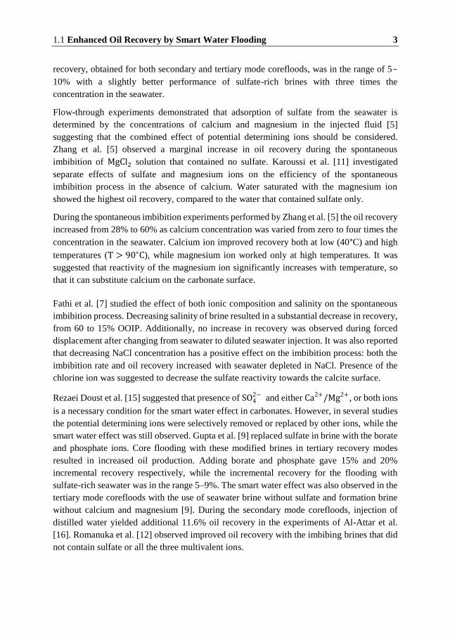
1.1 Enhanced Oil Recovery by Smart Water Flooding 3

recovery, obtained for both secondary and tertiary mode corefloods, was in the range of 5-

10% with a slightly better performance of sulfate-rich brines with three times the

concentration in the seawater.

Flow-through experiments demonstrated that adsorption of sulfate from the seawater is

determined by the concentrations of calcium and magnesium in the injected fluid [5]

suggesting that the combined effect of potential determining ions should be considered.

Zhang et al. [5] observed a marginal increase in oil recovery during the spontaneous

imbibition of MgCl2 solution that contained no sulfate. Karoussi et al. [11] investigated

separate effects of sulfate and magnesium ions on the efficiency of the spontaneous

imbibition process in the absence of calcium. Water saturated with the magnesium ion

showed the highest oil recovery, compared to the water that contained sulfate only.

During the spontaneous imbibition experiments performed by Zhang et al. [5] the oil recovery

increased from 28% to 60% as calcium concentration was varied from zero to four times the

concentration in the seawater. Calcium ion improved recovery both at low (40°C) and high

temperatures (T > 90∘C), while magnesium ion worked only at high temperatures. It was

suggested that reactivity of the magnesium ion significantly increases with temperature, so

that it can substitute calcium on the carbonate surface.

Fathi et al. [7] studied the effect of both ionic composition and salinity on the spontaneous

imbibition process. Decreasing salinity of brine resulted in a substantial decrease in recovery,

from 60 to 15% OOIP. Additionally, no increase in recovery was observed during forced

displacement after changing from seawater to diluted seawater injection. It was also reported

that decreasing NaCl concentration has a positive effect on the imbibition process: both the

imbibition rate and oil recovery increased with seawater depleted in NaCl. Presence of the

chlorine ion was suggested to decrease the sulfate reactivity towards the calcite surface.

Rezaei Doust et al. [15] suggested that presence of SO42− and either Ca2+/Mg2+, or both ions

is a necessary condition for the smart water effect in carbonates. However, in several studies

the potential determining ions were selectively removed or replaced by other ions, while the

smart water effect was still observed. Gupta et al. [9] replaced sulfate in brine with the borate

and phosphate ions. Core flooding with these modified brines in tertiary recovery modes

resulted in increased oil production. Adding borate and phosphate gave 15% and 20%

incremental recovery respectively, while the incremental recovery for the flooding with

sulfate-rich seawater was in the range 5–9%. The smart water effect was also observed in the

tertiary mode corefloods with the use of seawater brine without sulfate and formation brine

without calcium and magnesium [9]. During the secondary mode corefloods, injection of

distilled water yielded additional 11.6% oil recovery in the experiments of Al-Attar et al.

[16]. Romanuka et al. [12] observed improved oil recovery with the imbibing brines that did

not contain sulfate or all the three multivalent ions.

4 Introduction

1.1.1.2 Effect of temperature

Temperature is an important parameter when considering most of the water-based EOR

techniques. The smart water effects in carbonates have been observed at temperatures below

90°C in spontaneous imbibition experiments [5, 17, 18]. However, increasing temperature

always resulted in a significant improvement in recovery [14, 19, 20]. Meanwhile, in the core

flood experiments temperature has a much less definite effect; some secondary and tertiary

core flood experiments showed no or only slight increase in recovery with temperature [8,

21].

It is also suggested that water-wetness of carbonate rocks increases with temperature [22].

Yu et al. [23] observed contact angle shifting from intermediate-wet to water-wet, as

temperature increased from 20 to 130°C, with seawater and seawater with four times more

sulfate. Zhang et al. [5] observed increased adsorption of sulfate from seawater in the flow-

through experiments on the outcrop chalk under increasing temperatures. Larger adsorption

of sulfate lowers the surface charge of the carbonate rock increasing its water-wetness.

1.1.1.3 Effect of low salinity

The low salinity water (LSW) was not considered as a possibility for EOR in carbonate rocks

for a long time. According to the explanation given by Lager et al. [24], LSW was proved to

be successful in sandstones with high clay content and, therefore, low salinity effects were

not expected to be observed in carbonates due to typically minimal presence of the clay

material. Recent studies, however, contradict this assessment.

Yousef et al. [25] performed flooding experiments on the composite limestone core plugs.

They applied a number of brines obtained by diluting the seawater and demonstrated that

sequential injection of diluted brine resulted in the recovery increase, after recovery plateau

was reached with the previously injected brine. Lowering the solution salinity had an effect

on the pressure in the core: an increase in pressure drop was observed when using low salinity

brines, which was explained by probable migration of fines.

Zahid et al. [21] performed coreflood experiments on both reservoir and outcrop chalk using

diluted seawater at high temperature. The overall efficiency of the seawater flooding of

Middle East reservoir chalk was relatively low with a recovery factor of around 30%.

Subsequent injection of the two and ten times diluted seawater yielded production of

additional 5-10% OOIP. Similar to the previous study, the pressure drop increased on the

injection of diluted brines. Meanwhile, increase of recovery was not observed for the outrcrop

chalk cores.

Romanuka et al. [12] carried out a series of spontaneous imbibition experiments using chalk,

limestone and dolomite core plugs. Application of brines with modified salinity demonstrated

significant variance in the magnitude of incremental recovery. Overall, it was concluded that

brines with a lower ionic strength promote recovery. It was observed that the chalk core plugs

1.1 Enhanced Oil Recovery by Smart Water Flooding 5

produce more oil in response to increasing sulfate concentration at high ionic strength, in

contrast to the behavior of limestone and dolomite.

1.1.1.4 Effect of oil properties

Strand et al. [4] used two different types of oil to study the impact of the oil acid number.

Increase in the acid number (AN) from 0.70 to 1.9 mg of KOH/g resulted in decrease of the

ultimate oil recovery by spontaneous imbibition from 30 to 10% OOIP. However, it was not

proved that ultimate recovery for the forced displacement is affected by the AN and

temperature, as most of the experiments were stopped before the recovery plateau was

reached. A larger increment in oil recovery with the use of oil with low AN was also observed

in several spontaneous imbibition experiments that were not directly addressing the

properties of oil [14].

Fathi et al. [26] studied the interaction of oil with the surface of chalk using two artificially

prepared oils different in the acid numbers (AN = 1.5 and 1.8 mg of KOH/g). During the

spontaneous imbibition, both the rate and the ultimate recovery were higher for the cores

saturated with oil depleted in the water soluble acids (low AN). It was concluded that oil

properties affect the wetting state of carbonate rocks mainly due to the presence of the

carboxyl groups in oil.

Zahid et al. [27] studied the interaction between the brine and Latin American oil and

observed a decrease in oil viscosity in contact with brine as the sulfate concentration was

increased. A possible explanation of this phenomena is a specific interaction of ions in the

solution with heavy components in oil (aromatics, asphaltenes) so that brine was acting like

a polymer. However, a particular mechanism that might explain the interaction of sulfate ions

with the crude oil was not identified. Additionally, formation of a new phase, probably an

emulsion, was observed during a similar experiment with the Middle East crude oil. The

conditions for formation of a stable emulsion were reported to be high temperature (110°C),

pressure (300 bars), and high concentration of sulfate.

Chakravarty et al. [28] conducted experiments to study a possibility and conditions for

emulsion formation between an oil and an aqueous solution. The mixtures of oil and brine

were stirred and left isolated for 18 hours to attain equilibrium. After an incubation period,

emulsions could be visually observed if the oil initially contained polar components. It was

suggested that heavier oil components participate in the formation of the emulsion.

Meanwhile, in the recent Master thesis of Jakub Benicek [29] it was demonstrated that it is

light oil components that participate in the formation of the emulsions. The problem needs

further study.

6 Introduction

1.1.1.5 Effect of rock material

Different mineralogical properties of carbonate rocks may affect the magnitude of response

to mechanisms underlying the smart water effects. The outcrop rocks are often used as

reservoir rock analogs. However, significant differences between them and the reservoir

rocks have been observed in several studies under the same experimental conditions.

Therefore, one should be careful when extending conclusions applicable to one rock type to

another.

Zahid et al. [30] performed coreflooding experiments on the North Sea reservoir and Stevns

Klint outcrop chalks. It was observed that the temperature increase did not have a significant

effect on the recovery from the reservoir rocks while flooding in the outcrop chalk was

strongly affected as the temperature was increased from 40 to 120°C. It was also reported

that increasing the sulfate concentration three times compared to the concentration in

seawater resulted in an increase of only 0.7 and 1.2% OOIP from the reservoir core, compared

to the recovery achieved the with sulfate free brine.

Spontaneous imbibition experiments performed by Fjelde et al. [31] on the two core plugs

from the fractured chalk field demonstrated an insignificant incremental recovery after

switching from sulfate-free formation brine to seawater, which was incomparable to the

apparent improvement observed in the Stevns Klint outcrop chalk. Fernø et al. [11] studied

the effect of sulfate concentration on the oil recovery during spontaneous imbibition in

Stevens Klint, Rørdal, and Niobrara outcrop chalks. Effect of increasing the sulfate

concentration was different for the three cores in study: no effect was observed in Rørdal and

Niobrara plugs, while in the Stevns Klint chalk the incremental recovery was smaller

compared to previously reported in other studies.

1.1.1.6 Summary

Available evidence suggests that potential determining ions have a strong effect on the

recovery from the carbonate rocks. Most of the published experimental data associate the

smart water effect with the wettability alteration towards increased water-wetness for

intermediate- and oil-wet carbonates. High temperature (T > 90∘C) strengthens the

magnitude of the smart water effect, especially in the spontaneous imbibition experiments.

Nevertheless, high temperature is not the necessary condition, since improved recovery with

seawater injection/imbibition has also been observed under low temperatures. Oil properties

affect the wetting state of the rock; large acid number of oil indicates a stronger interaction

between the polar oil components and the carbonate surface. A positive effect on recovery

by seawater flooding and imbibition has been observed both in chalk, limestone and dolomite

reservoir and outcrop chalk. However, in several experiments behavior of reservoir and

outcrop cores was much different, and there is yet no explanation for the observed deviating

behavior.

1.1 Enhanced Oil Recovery by Smart Water Flooding 7

1.1.2 Recovery Mechanisms

1.1.2.1 Multi-ion exchange

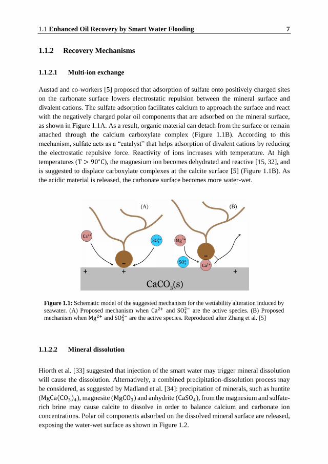
Austad and co-workers [5] proposed that adsorption of sulfate onto positively charged sites

on the carbonate surface lowers electrostatic repulsion between the mineral surface and

divalent cations. The sulfate adsorption facilitates calcium to approach the surface and react

with the negatively charged polar oil components that are adsorbed on the mineral surface,

as shown in Figure 1.1A. As a result, organic material can detach from the surface or remain

attached through the calcium carboxylate complex (Figure 1.1B). According to this

mechanism, sulfate acts as a “catalyst” that helps adsorption of divalent cations by reducing

the electrostatic repulsive force. Reactivity of ions increases with temperature. At high

temperatures (T > 90∘C), the magnesium ion becomes dehydrated and reactive [15, 32], and

is suggested to displace carboxylate complexes at the calcite surface [5] (Figure 1.1B). As

the acidic material is released, the carbonate surface becomes more water-wet.

1.1.2.2 Mineral dissolution

Hiorth et al. [33] suggested that injection of the smart water may trigger mineral dissolution

will cause the dissolution. Alternatively, a combined precipitation-dissolution process may

be considered, as suggested by Madland et al. [34]: precipitation of minerals, such as huntite

(MgCa(CO3)4), magnesite (MgCO3) and anhydrite (CaSO4), from the magnesium and sulfate-

rich brine may cause calcite to dissolve in order to balance calcium and carbonate ion

concentrations. Polar oil components adsorbed on the dissolved mineral surface are released,

exposing the water-wet surface as shown in Figure 1.2.

Figure 1.1: Schematic model of the suggested mechanism for the wettability alteration induced by

seawater. (A) Proposed mechanism when Ca2+ and SO42− are the active species. (B) Proposed

mechanism when Mg2+ and SO42− are the active species. Reproduced after Zhang et al. [5]

SO

(A) (B)

Ca

-

Mg

CaCO3(s)

+ + + Ca

SO

-

8 Introduction

1.1.2.3 Mineral fines migration

Tang and Morrow [35] observed the fines migration and stripping of oil-wetted particles from

rock surfaces in sandstones during LSW. The release of these particles has a double effect;

first, it improves the water-wetness of the rock and, second, the mineral fines flowing along

an established flow path plug pore throats, increasing the sweep efficiency. Rezaei Doust et

al. [15] suggested that diversion of the original flow paths is more important than wettability

modification by the fines release. Blocking the pore throats decreases the permeability that

can be observed by increasing pressure drop [21, 36, 37].

Possible sources of mineral particles are precipitation of solids from the saturated solution

and detachment of the minerals from the rock. Chakravarty et al. [38] suggested that the ion

substitution of calcium by magnesium on the carbonate surface can result in significant

increase of Ca2+ concentration in the brine and trigger precipitation of anhydrite forming

mineral fines. Chakravarty et al. [28] speculated that fines interact with crude oil polar

components, which results in a formation of the water-soluble stable oil emulsion.

1.1.2.4 Double layer expansion

This mechanism was suggested by Ligthelm et al. [39]. The thickness of the electric double

layer between the rock surface and the formation brine is reduced during injection/imbibition

of the seawater in a core. This is due to typically large ionic strength of the formation brines

resulting in compaction of the counter-ions in the diffuse layer. When the electrolyte

concentration in brine is reduced, the screening potential from the ions is lowered, which

causes the electrical double layers surrounding the mineral surface and oil droplets to expand.

The repulsion force between the surface and droplets increases, which provokes liberation of

the oil droplets. The effect is expected to be more pronounced during the LSW.

Figure 1.2: Top: A section of the pore space before any dissolution reaction. The surface is rough,

and oil is attached where there is a large curvature and the water film is broken. Bottom:

Dissolution of the chalk surface has taken place where the oil was attached, and new water-wet

rock surface has been created. Reproduced after Hiorth et al. [33]

Oil

Aqueous phase

Dissolution

Rock Surface

Water wet

1.2 Low Salinity Waterflooding (LSW) in Sandstones 9

1.2 Low Salinity Waterflooding (LSW) in Sandstones

The effect of water salinity on the recovery from the clay-bearing sandstone rocks was first

reported in the 1960s [40]. However, this effect has not received proper attention in the

subsequent years. The effect was later rediscovered by Morrow and co-workers [41-43],

whose experiments demonstrated that oil recovery is influenced by the composition of the

injected water. Further research in this area revealed the strong effect of brine salinity on the

oil recovery [35, 44]. The interest in the low salinity waterflooding has increased drastically

in the recent decades, resulting in a significant number of publications.

1.2.1 Conditions for the Low Salinity Effects

Based on the systematic experimental work of the different research groups, Rezaei Doust et

al. [15] formulated the following conditions necessary for the low salinity effects in

sandstones:

Porous medium

― Clay must be present in the formation. A type of the clay may also

influence the effect.

Oil

― Oil must contain polar components (acid or base). No effects have been

observed in experiments with the refined oil.

Water

― Initial formation water (FW) must be present.

― The formation water must contain divalent cations such as Ca2+ and Mg2+.

― Salinity of the injected fluid should be in the range of 1000–2000 ppm.

― Ionic composition of the injected fluid is important (Ca2+ vs Mg2+).

Production/migration of fines

― In some cases, fines were produced during the LSW, but the effect of LSW

was also demonstrated in the cases where no fines were observed.

Permeability decrease

― Pressure drop increased in the most experiments, which may be related to

the migration of fines or formation of emulsions.

Temperature

― Temperature does not seem to play any clear role. However, the

experiments were performed mostly at temperatures below 100°C.

Low salinity effects have been observed both in the secondary and the tertiary recovery

modes. The oil recoveries from the two schemes are in general comparable.

10 Introduction

1.2.2 Mechanisms of LSW

Though a large amount of experimental data is available to judge on the possible mechanisms

behind the low salinity effects in sandstones the full understanding of the process has not

been achieved yet. As a result, a large number of possible explanations have been proposed,

but none of them has commonly been accepted. Probably, the reason is that the different

mechanisms work and interact, and the contribution of each mechanism depends on a

particular choice of the crude oil/brine/rock system. Thus, a dominant mechanism may vary

from one experiment to another. Below we provide a brief overview on some of the proposed

mechanisms.

1.2.2.1 Migration of fines

It was suggested by Tang and Morrow [35] that the decreased salinity of the injected water

may affect stability of clays, which may disintegrate due to swelling. Release of clay

fragments (fines) will produce the two important effects. First, release of oil-wet fines from

the surface will increase its wetness; secondly, fines can migrate and block pore throats,

damaging the permeability and diverting the flow.

1.2.2.2 IFT reduction

McGuire et al. [45] proposed that low salinity mechanism may work similarly to alkaline

flooding, resulting in the increased pH and reduced interfacial tension (IFT). This is

especially valid under high pH conditions, as organic acids in crude oil react to produce in

situ surfactant, lowering the IFT. Such conditions are favorable for formation of oil/water or

water/oil emulsion, which may improve the sweep efficiency.

1.2.2.3 Multicomponent ion exchange (MIE)

The mechanism of multicomponent ion exchange is based on an assumption that wetting

properties of rocks are controlled by the ions that are adsorbed in the core on the clay patches.

Lager et al. [24] proposed that divalent cations play a significant role in the interaction

between the polar components in the oil and the clay minerals. In the proposed model Ca2+

acts as a ”bridge” between the negatively charged clay surface and the carboxylic material.

Due to injection of the low salinity water Ca2+–carboxyl complexes gain an ability to desorb

from the surface.

1.2.2.4 The salting-in mechanism

This mechanism is an opposite to the known salting-out effect, according to which solubility

of the organic material in the presence of salt decreases. Rezaei Doust et al. [15] proposed

1.3 Modeling of the Smart Water Effects 11

that removing salt from the water may have an opposite effect. Therefore, decreasing salinity

below a critical ionic strength increases solubility of the organic material in the brine, so that

oil recovery is improved.

1.3 Modeling of the Smart Water Effects

The progress in the experimental investigation of the smart water effects demanded a

development of an appropriate mathematical model to reproduce the experimental

observations and to propose a quantitative description of these effects.

One of the first approaches was developed by Jerauld et al. [46] to describe the low salinity

effect. Using the injected brine salinity as a governing parameter, Jerauld et al. performed an

interpolation of the relative permeability and the capillary pressure curves as a weighted

average of their values for high salinity (HS) and low salinity (LS) waterflooding. The

weighting function was calculated according to

LSorw orwHS LSorw orw

S S

S S (1.1)

where 𝑆𝑜𝑟𝑤 is the residual oil saturation for a given salinity, which in turn was linearly

interpolated between the low salinity and the high salinity residual oil saturations.

Mahani et al. [47] used a similar approach based on the interpolation of the relative

permeabilities. The main difference comes from the shape of the interpolation function; it

was suggested that wettability changed abruptly as a threshold value of the mixing factor is

achieved. The threshold mixing factor 𝑓 was defined according to

*FW

FW LS

TDS TDSfTDS TDS

(1.2)

Where 𝑇𝐷𝑆𝐹𝑊 and 𝑇𝐷𝑆𝐿𝑆 are the salinities of the formation (high salinity) brine and the

injected (low salinity) brine, while 𝑇𝐷𝑆∗ is the threshold salinity. The estimated value for 𝑓

was above 0.9 meaning that very high dilution of the HS formation water was required to

induce the wettability alteration. The model was partly capable of reproducing the history of

production.

Omekeh et al. [48, 49] introduced the effect of the multicomponent ion exchange to model

the low salinity flooding in clay-bearing sandstone rocks. The model accounted for the

adsorbed cationic surface species that were in equilibrium with the ions in the bulk solution.

Omekeh et al. performed an interpolation of relative permeabilities based on the change in

composition of the surface using the weight function 𝐻 defined as follows:

12 Introduction

,

1( , )

1 max( ,0)Ca Mg I

i ii Ca Mg

Hr

(1.3)

where 𝑟 is the constant determining the shape of the interpolating function, and 𝛽𝑖 are the

equivalent fractions of the adsorbed species. The model was applied in order to confirm the

MIE mechanism and could reproduce some of the experimnetal data.

Dang et al. [50, 51] implemented multicomponent ion exchange in the compositional

simulator GEM™, which also included various geochemical interactions and aqueous

chemistry, together with the possibility to model the WAG displacement.

Hiorth et al. [52, 53] developed a mathematical model of the calcite surface in equilibrium

with an aqueous solution. The model incorporated surface complexation and bulk chemistry.

It was demonstrated that the model can be used to predict the surface charge of calcite in

brine and the sulfate adsorption on calcite by modeling of the zeta potential data [14] and

adsorption data [54]. The simulation results also indicated that variation of the surface charge

could not explain the observed oil recovery increase with temperature, as observed under

spontaneous seawater imbibition [5, 14], while the correlation between oil recovery and the

chalk dissolution demonstrated a good agreement.

Brady et al. [55] developed a surface complexation model to study the equilibrium between

a modeled oil, calcite surface and aqueous solution as a function of temperature and brine

composition. Based on the performed modeling, it was concluded that the divalent potential

determining ions: SO42−, Ca2+, and Mg2+ reduce electrostatic complexation between the

negatively charged carboxyl groups present in the oil and the positively charged surface sites.

The study focused on surface complexation and did not consider dissolution and precipitation

processes. Nonetheless, the authors claimed a reasonable success in correlating their

predictions of complexation to the recovery trends observed in the available body of

spontaneous imbibition experiments.

Zaretskiy [56] developed a mathematical model of calcite in equilibrium with an aqueous

solution, following the approach introduced by Hiorth et al. [52]. The main difference came

from incorporation of a 1D single-phase flow model, which allowed to consider rate-

dependent effects. The study successfully reproduced some of the coreflood experiments [5,

32, 57] and showed that both rock dissolution and ion adsorption should be considered in

modeling the spontaneous imbibition experiments. Presence of the oil phase was not

considered in this study.

1.4 Objectives 13

1.4 Objectives

The overall objective of this work is to investigate how different mechanisms influence the

oil recovery, pressure distribution and composition of the brine during the smart water

flooding in oil saturated rocks. Based on the overview of the experimental work, it may be

concluded that yet there is no complete understanding of the mechanisms underlying the

smart water effects.

A general approach, used for the modeling of EOR processes, involves interpolation of the

relative permeability functions and capillary pressure curves based on a governing parameter.

A challenge in modeling of the smart water phenomena is that such parameters are difficult

to identify, unlike in the conventional chemical waterflooding. As suggested by the different

works on the smart water effect in carbonates, both surface complexation and mineral

dissolution models could be successfully applied to the same experimental data. Therefore,

it is necessary to consider not only ultimate recovery, but also other available experimental

data, such as pressure distribution and ion concentrations in the effluent brine. Analysis of

the produced brine composition should be performed in order to improve our knowledge of

the thermodynamic parameters used to describe the crude oil/brine/rock interactions as in

general there is a large uncertainty in such data.

An additional challenge comes from considering the tertiary flooding. It is known that oil

trapped in the swept zones inside porous media is present in a form of disconnected oil drops,

or oil ganglia. Therefore, the general modeling approach based on interpolation of relative

permeability curves should be avoided or used with caution. Considering oil ganglia, it is

important to understand the mechanisms that can cause their mobilization and the

mechanisms that govern their transport in porous media. The macroscopic theory of

multiphase flow assumes that fluid phases flow in their own pore networks and do not

influence each other. It is doubtful that the same assumption may be applied for a flow of a

single oil ganglion surrounded by water in the pore space. Therefore, an alternative

description should be developed.

1.5 Outline

This rest of the thesis is structured as follows. Chapter 2 provides theory necessary for the

development of the models of macroscopic multiphase flow in porous media accounting for

the geochemical interactions. A specific attention is paid to the surface chemistry of chalks.

Description of the numerical methods applied for modeling is given in Chapter 3. We stick

to a general formulation of the system of conservation laws and flow equations for the

reactive multiphase multicomponent transport applicable in multiple dimensions and

describe numerical approaches that are implemented in our modeling. In Chapter 4 we

present a study of the mineral dissolution and its possible effects on the waterflooding. The

14 Introduction

study focuses on the porosity/permeability alteration due to dissolution and effects of mass

transfer on pressure distribution. Chapter 5 presents the development of a micromodel for the

two-phase flow on a level of the single pore represented by an angular capillary. In Chapter

6, we present a new formalism to take into account effects that might arise during tertiary

waterflooding. We develop a description of the flow of the oil phase consisting of separate

oil ganglia that can be mobilized and flow due to wettability alteration. We conclude the

Chapter with numerical modeling of a tertiary recovery process to investigate the possible

outcomes of the model. In Chapter 7 we revise available experimental data on the single- and

two-phase flooding in chalk to understand what physicochemical effect(s) can explain these

measurements. We develop a mathematical model that takes into account interaction between

carbonate surface and the aqueous solution and perform numerical modeling to of the smart

water flooding experiments. The Conclusions and Suggestions for Future Work are given in

Chapter 8.

1.6 Publications

The work performed during this Ph.D. study has led to a two publications so far. The work

presented in Chapter 4 on the modeling of dissolution effect on waterflooding resulted in the

following article:

Artem Alexeev, Alexander Shapiro, and Kaj Thomsen. Modeling of dissolution

effects on waterflooding. Transport in Porous Media, 106(3):545–562, 2015.

Part of the work presented in Chapter 5 on the microscopic model for the two-phase flow and

Chapter 6 on the mobility of oil ganglia led to a publication of the following article:

Artem Alexeev, Alexander Shapiro, and Kaj Thomsen. Mathematical Model for

Tertiary Recovery by Mobilization of Oil Ganglia. (Submitted to Transport in

Porous Media)

2

2 Theory

This chapter covers the standard theory regarding two-phase flow in porous media. The

structure of this Chapter is the following. In Section 2.1, we introduce basic concepts that

describe crude oil/brine/rock (CBR) system. Next, in Section 2.2, we describe the most

important geochemical interactions, relevant to the smart water flooding. In Section 2.3, we

describe the Buckley-Leverett model for linear flooding and give an overview on some of

the known analytical solutions.

2.1 Wettability

Wettability is defined as a tendency of one fluid to adhere to a solid surface in the presence

of other immiscible fluids. As applied to the petroleum industry, it describes a preference of

the reservoir rock to be in contact with either water, or oil, or both. This is illustrated in Figure

2.1. It is important to note that wettability only determines the wetting preference of the rock,

but does not directly refer to the fluid that is in contact with the rock. Specific crude

oil/brine/rock interactions may result in wettability ranging from strongly water-wet to

strongly oil-wet. Intermediate (or neutral) wettability corresponds to a case when rock has no

strong preference to any of the fluids.

Due to complex nature of the reservoir rocks, they can also develop fractional wettability.

The internal surface of the rock is composed of many minerals with different chemical and

adsorption properties. Thus, adsorption of crude oil components on some areas of the rock

may result in heterogeneous or spotted wettability. Mixed wettability, as introduced by

Salathiel [58], is a special case of the fractional wettability in which the oil-wet surfaces form

continuous paths through larger pores. It is assumed that in mixed-wet rocks water has a

tendency to occupy small pores, which remain water wet while oil occupies larger pores [59].

Wettability is one of the major factors that affects flow and distribution of fluids in porous

media. Therefore, it is important to be able to ”measure” wettability and understand the

mechanisms that may alter the wetting state of the rock.

A measure of wettability is the contact angle 𝜃, which arises because of the action of the

interfacial tension on the interphase boundaries, as illustrated in Figure 2.1b. General

characterization of the rock wettability according to Anderson [59] is the following: for a

water-wet rock 𝜃 < 75∘, for an oil-wet rock 𝜃 > 105∘, while the range 75∘ < 𝜃 < 105∘

corresponds to neutral wet rocks. However, several factors limit the application of contact

16 Theory

angle measurements to characterize wettability. First, the measurements are usually

performed on a smooth surface, and cannot take into account roughness, heterogeneity and

complex geometry of the reservoir rocks [60]. Second, the contact angle provides no

information about the presence of permanently attached organic material on reservoir rocks.

For the mentioned reasons, characterization of wettability of the core with the contact angles

is not complete, and other techniques are to be considered.

2.1.1 Capillary pressure

The action of interfacial tension on the interface of the two immiscible liquids results in the

pressure difference in the liquids, known as capillary pressure. The capillary pressure is

calculated according to the Laplace equation:

1 2

1 1c non wetting wetting owP P P

r r (2.1)

where 𝛾𝑜𝑤 is the surface tension, and 𝑟1, 𝑟2 are the principal radii of the surface curvature.

For a meniscus inside a cylindrical capillary, which may be considered as a representation of

single pore, the capillary pressure is calculated according to the Young-Laplace equation

2 cosowcP r

(2.2)

where r is the capillary radius.

Considering the capillary pressure difference arising in porous media, one need to take into

account the pore size distribution, interfacial tension, wetting conditions, and saturation.

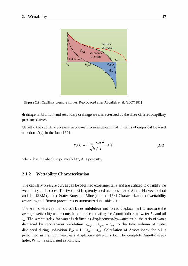
However, it turns out that capillary pressure is also determined by the saturation history [59].

This principle is illustrated in Figure 2.2: the three different displacement processes: primary

Figure 2.1: Examples of different wettability conditions: a) strongly water-wet; b) water-wet; c)

strongly oil-wet. Reproduced after Abdallah et al. [61]

𝛾 𝑤

𝛾 𝑜

𝛾𝑜𝑤

Oil

Rock

Watera) b) c)

2.1 Wettability 17

drainage, imbibition, and secondary drainage are characterized by the three different capillary

pressure curves.

Usually, the capillary pressure in porous media is determined in terms of empirical Leverett

function ( )J s in the form [62]:

cos( ) ( )

/ow

cP s J sk

(2.3)

where 𝑘 is the absolute permeability, 𝜙 is porosity.

2.1.2 Wettability Characterization

The capillary pressure curves can be obtained experimentally and are utilized to quantify the

wettability of the cores. The two most frequently used methods are the Amott-Harvey method

and the USBM (United States Bureau of Mines) method [63]. Characterization of wettability

according to different procedures is summarized in Table 2.1.

The Ammot-Harvey method combines imbibition and forced displacement to measure the

average wettability of the core. It requires calculating the Amott indices of water 𝐼𝑤 and oil

𝐼𝑜. The Amott index for water is defined as displacement-by-water ratio: the ratio of water

displaced by spontaneous imbibition 𝑉𝑤 𝑝 = 𝑠 𝑝𝑤 − 𝑠𝑤𝑖 to the total volume of water

displaced during imbibition 𝑉𝑤𝑡 = 1 − 𝑠𝑜𝑟 − 𝑠𝑤𝑖 . Calculation of Amott index for oil is

performed in a similar way, as a displacement-by-oil ratio. The complete Amott-Harvey

index WI𝐴𝐻 is calculated as follows:

Figure 2.2: Capillary pressure curves. Reproduced after Abdallah et al. (2007) [61].

𝑠𝑤𝑖

𝑠𝑜𝑟

Primary drainage

Secondary drainage

Imbibition

𝑠 𝑝𝑤 𝑠 𝑝𝑜

𝑤

𝑜

18 Theory

WI

,1 1

AH w o

spw wi or spow o

or wi or wi

I I

s s s sI I

s s s s

(2.4)

where 𝑠 𝑝𝑤 is the water saturation for zero capillary pressure during the imbibition process,

and 𝑠 𝑝𝑜 is the oil saturation for a zero capillary pressure during the secondary drainage, as

shown in Figure 2.2. The Amott-Harvey index changes between +1 for strongly water-wet

rocks and -1 for strongly oil-wet rocks. The main shortcoming of this method is its

insensitivity close to neural wetting conditions [64]. In addition, there is no standard time

allowing spontaneous imbibition to occur (it may proceed for several months) and if the

imbibition is stopped after a short period of time, the resulting wettability index will

underestimate the water or the oil-wetness of the rock.

Calculation of the USBM index is based on the work required to displace the non-wetting

phase. It has been shown that this work is proportional to the area under the capillary pressure

curves corresponding to imbibition and drainage [59]. These areas Aw and Ao are marked in

Figure 2.2 for a combined Amott/USBM method. According to the procedure, the USBM

index WI𝑈𝑆𝐵𝑀 is calculated as

WI ln( / )USBM w oA A (2.5)

The USBM wettability index is not bounded and can take any value between −∞ and +∞.

Practically, WI𝑈𝑆𝐵𝑀 is around 0 for neutral wet cores, and ±1 for strongly water-wet and oil-

wet cores correspondingly. The main advantage of the USBM test is its sensitivity near

neutral wettability; however, it cannot determine whether a system has a fractional or mixed

wettability, while the Amott test is sometimes sensitive to that [59].

Recently Strand et al. [54] proposed a new method to calculate the wettability index of

carbonates based on chromatographic separation between sulfate and thiocyanate (SCN−).

Due to adsorption of sulfate on the surface of calcite, production of sulfate in the effluent is

delayed compared to SCN−. This adsorption takes place only on the water-wet pore surface

and the fraction area covered by water is assumed to represent the new wettability index:

Wett

Heptane

WINewA

A (2.6)

where AWett and AHeptane are the calculated areas between the SO42− and SCN− effluent

concentration curves for a core in study and a reference core containing heptane, which is

assumed to be completely water-wet. The range of this wetting index is from 0 for a

completely oil-wet core to 1 for a completely water-wet core. An advantage of this method

is good sensitivity of the wetting index in the total wetting range, and, in particular, its

2.1 Wettability 19

sensitivity close to neutral wetting conditions. Additionally, the method is robust as it does

not involve long-term imbibition tests.

2.1.3 Effect on Displacement

According to the description given by Craig [66], in a strongly water-wet rock, water

occupies smaller pores and forms a thin film covering the entire surface. Oil fills centers of

the larger pores. During flooding, oil is displaced from the centers of some pores while in

other pores it finds its way along the surface of the rock (e.g. corner filaments). This may

result in considerable trapping, by a mechanism known as snap-off [67]. Consider water

traveling around the exterior of a pore and bypassing the non-wetting oil phase in the center.

On reaching the exit throat of the pore, capillary instability may result in cutting (snapping

off) the oil connection in that pore throat. The trapped oil will remain immobile due to the

action of capillary forces. The disconnected residual oil is present in the two different forms:

(1) small oil drops in the centers of larger pores and (2) larger patches of oil extending over

several pores, but disconnected from the effluent [68]. Thus, in strongly water-wet rocks,

trapping is controlled by the capillary forces, and most of the trapping occurs immediately

after passage of a displacement front. As a result, a large fraction of oil is produced before

the water breakthrough, while very little additional oil is produced after the breakthrough

[69].

In an oil-wet rock, oil covers the rock surface. During flooding, water flows through the

larger pores bypassing the smaller ones. This displacement pattern results in an earlier

breakthrough compared to the water-wet rock. Since oil phase remains connected, it can be

displaced from the reservoir for a long time. However, efficiency of such displacement is

low, since it is required to inject large amounts of water to reach a reasonable recovery. This

makes waterflooding in the oil-wet systems less efficient than waterflooding in the water-wet

systems [65].

Recovery both from water-wet and oil-wet rocks is challenging, and it is sometimes assumed

that intermediate-wet conditions are more favorable for the waterflooding. The neutral

wettability is expected to result in less trapping, compared to water-wet conditions and reduce

Table 2.1: Approximate relationships between wettability, contact angle and the USBM and Amott-

Harvey wettability indexes [65].

Water-wet Neutral wet Oil-wet

𝜃 0 75 75 105 105 180

WI𝐴𝐻 WI3 .0. 1 0 WI0 3 0.. 3 WI 00 .1 3.

WI𝑈𝑆𝐵𝑀 ≈ 1 ≈ 0 ≈ −1

WI𝑁𝑒𝑤 ≈ 1 ≈ 1/2 ≈ 0

20 Theory

the tendency of water to bypass oil through large pores compared to oil-wet conditions.

However, the real pattern is more complicated and as pointed out by Anderson [69] in some

experiments the residual oil saturation was insensitive to the wetting conditions while in other

strong water wet conditions resulted in lower residual oil saturation.

2.1.4 Change of Wettability

Most of the clean sedimentary rocks are strongly water-wet. For that reason, historically, it

was assumed that water films prevent oil from touching the surface of the reservoir rock [59].

This turned out not to be true, as strong water-wetness can be altered by the adsorption of

polar compounds from oil and deposition of organic matter. The surface active agents in oil

contain both polar and hydrocarbon ends. When the polar compound is adsorbed, the

hydrocarbon end is exposed, making the surface more oil-wet. The adsorption of polar

compounds occurs preferentially on the surface of the opposite polarity: acidic compounds

are adsorbed on the positively charged surface while basic compounds are adsorbed on the

negatively charged surfaces.

Adsorption of polar compounds, which are sufficiently soluble in water, can occur through

water films on the surface. Presence of wetting film may reduce but not completely inhibit

this adsorption process [59]. Reduction of the water film thickness eventually results in the

film rupture allowing oil to contact the rock. The water film is stabilized by the electric forces

arising from the electric double layer at the oil/water and water/rock interfaces. Therefore,

brine chemistry also affects the wettability of the rock. All the factors, inducing brine pH,

salinity, and ionic composition have an effect on the properties of the electric double layer

and are expected to affect the adsorption of polar compounds from oil. Specific ions from

brine can also adsorb on the surface of the rock. These ions are called the potential

determining ions due to their ability to change the surface potential. The potential

determining ions for the carbonate surface are SO42−, Ca2+ and Mg2+ [3].

To account for the possible change of wettability during waterflooding, it is important to

understand what crude oil/brine/rock interactions occur in the system and what are their

potential effects on the waterflooding process on the whole.

2.2 Crude Oil/Brine/Rock Interactions

As it was previously stated, the main difference between conventional flooding and the smart

water flooding is that the latter is accompanied by various geochemical and fluid-fluid

interactions, including intra-aqueous reactions, mineral dissolution and precipitation,

adsorption of ions from the aqueous solution and polar components from oil on the surface

of the rock.

2.2 Crude Oil/Brine/Rock Interactions 21

2.2.1 Dissolution and Precipitation

Dissolution and precipitation processes are of major importance when considering the brine

composition both in the smart water (high/low salinity) and conventional floodings. Even

before smart waterflooding was introduced, the quality of water was analyzed in the industry.

Precipitation could cause a risk of formation damage and scaling [70].

The effect of dissolution and precipitation was mostly studied in connection with changes of

porosity, permeability and mechanical properties of the rock. For smart waterflooding,

dissolution and precipitation may also be considered as an internal source/sink for the ions

that contribute to the smart water effect.

Primary minerals comprising carbonate rocks are calcite and dolomite. Other important

minerals are gypsum (at low temperatures) and anhydrite (at high temperatures), because

Ca2+ and SO42− are readily present in seawater.

2.2.1.1 Calcite

Calcite can dissolve according to the following dissolution equilibrium reaction

2 23 3CaCO Ca CO (2.7)

This equation describes the dissolution process in distilled water in the absence of carbon

dioxide. However, a complete picture of calcite dissolution is more complicated, since one

need to account for proper aqueous chemistry. The overall dissolution reaction, in this case,

can be represented by

2 23 2 2 3CaCO H O+CO (g) Ca 2HCO (2.8)

Equation (2.8) reflects the relation between the carbon dioxide and the calcite dissolution.

Plummer et al. [71] developed a rate model for calcite dissolution based on three mechanisms

of the dissolution reaction:

21 2 2 3 3 2 4 3[H ] [H CO ] [H O] [Ca ][HCO ]

f b

calcite

r r

r k k k k (2.9)

where 𝑟𝑐𝑎𝑙𝑐𝑖𝑡𝑒 is the specific rate of calcite dissolution, [… ] represent the activities of aqueous

species and 𝑘𝑖 = 𝑘𝑖(𝑇), are the rate constants fitted to experimental data. The effect of the

first term is significant only at pH values lower than 3.5. While 𝑘1, 𝑘3 do not vary

significantly is the range of temperatures used for smart water experiments, 𝑘2 and 𝑘4

increase significantly with temperature [72], and the corresponding terms in the kinetic

equations are the most important in determining the rate of dissolution. The value [H2CO3]

represents the activity of CO2(𝑎𝑞) and is related to the carbon dioxide pressure. Thus, carbon

22 Theory

dioxide controls the calcite equilibria. Pokrovsky et al. [73], proposed the following

polynomial empirical relation to estimate the calcite dissolution rate:

2 2

2CO COlog ( )fr A B P C P (2.10)

where 𝑃CO is the carbon dioxide pressure and A, B and C are the temperature dependent

parameters calculated from fitting the experimental data.

2.2.1.2 Dolomite

The following reaction describes the dissolution of dolomite in water:

2 23 2 2 2 3CaMg(CO ) 2CO ( ) 2H O Ca Mg 4HCOg (2.11)

Similarly to calcite, the pressure of carbon dioxide controls the process of dolomite

dissolution. The dissolution rate of dolomite is an order of magnitude lower than the

dissolution rate of calcite [72] and it is not expected to have any influence on the short-lasting

waterflooding experiments.

2.2.1.3 Anhydrite

As mentioned earlier, formation of anhydrite may occur under seawater injection into a

reservoir, especially at elevated temperatures. The reason is that solubility of anhydrite

drastically decreases with temperature, as shown in Figure 2.3. The following reaction

describes the anhydrite dissolution/precipitation process:

2 24 4CaSO Ca SO (2.12)

One should expect that increasing the temperature may result in anhydrite precipitation that

will lower the concentrations of Ca2+ and SO42−. Vice versa, during injection of a low salinity

brine, one should expect anhydrite dissolution to occur and increase the concentrations of

Ca2+ and SO42−.

The rate of anhydrite precipitation is a difficult parameter to determine. A primary difference

between calcite and anhydrite is their distribution within the porous media. Calcite is

abundant, whereas anhydrite is not always present. Formation of a crystal starts with a

nucleation, which is delayed by the so-called induction time dependent on the

thermodynamic conditions [74]. Thus, concerning precipitation of anhydrite in a core or a

reservoir it is hard to determine when and where it will start.

2.2 Crude Oil/Brine/Rock Interactions 23

2.2.1.4 Rates of Non-Equilibrium Reactions

The following expression is usually applied to calculate the rate of mineral dissolution and

precipitation reactions [75]:

(1 SI)ˆ nrr k A (2.13)

Here 𝑘 is the rate constant, is the reactive specific surface area, SI is the saturation index

SI = 𝐼 𝑃/𝐾 𝑝 , 𝐼 𝑃 stands for the ion activity product and 𝐾 𝑝 is the solubility product, 𝑛

is the parameter that is fitted in order to match the observed rates. These parameters are not

unique as they indirectly include the effects of surface heterogeneity and competition

between the convective and diffusive transport [75].

Alternatively, the rate law for the mineral dissolution/precipitation reaction may be

determined in the same way as it was introduced for the calcite dissolution in (2.9):

( )ˆ nf br k IAP k IAA P (2.14)

Where 𝑘𝑓 and 𝑘𝑏 are the forward and backward reaction rate constants respectively. Consider

the mineral reaction represented by

1

X 0spn

a aa

(2.15)

Figure 2.3: Solubility of CaSO4 as a function of temperature at pressure of 30 bar (black) and 300

bar (red) according to Extended UNIQUAC model.

0

500

1000

1500

2000

2500

3000

30 50 70 90 110 130

Ca

SO

4p

pm

Temperature C

30 bar

300 barCaSO4·2H2O

CaSO4

24 Theory

where 𝜈𝑎 are the stoichiometric coefficients for the species X𝑎. The stoichiometric

coefficients are such that 𝜈𝑎 < 0 for the reactants, and 𝜈𝑎 > 0 for the products. Then the ion

activity products are calculated as follows:

0 0

[X ] , [X ]

/

sp sp

a a

a a

n n

a aIAP IAP

IAP IAP IAP

(2.16)

The rate constant 𝑘 used in equations (2.13) and 𝑘𝑓 in equation (2.15) are not necessarily the

same. In fact, the parameters used in (2.13), (2.15) may not be considered as tabulated

constants. Most of the studies on the mineral dissolution rates are performed using the bulk

powder experiments, and a large variation in the rate constants is observed in different

experiments, especially where the different measurement techniques are applied [76].

2.2.2 Sorption

It is important to consider sorption of aqueous species on the surface of the rock. Due to large

surface area and, usually, high reactivity of the surface, it can adsorb considerable amounts

of the substances [77]. Below we consider several important models of sorption and ion

exchange that find its application in the modeling of the smart water flooding.

2.2.2.1 Henry adsorption isotherm

The linear Henry adsorption isotherm is one of the most widely applied models in

environmental geochemistry to predict sorption. It is also known as the distribution

coefficient approach [75]. This sorption model is based on the assumption that the ratio of

the sorbed to the dissolved mass of the component is determined by the Henry adsorption

constant (or the distribution coefficient):

/dK c c (2.17)

where 𝑐∗ is the concentration per bulk volume in mol/l(core), 𝑐 is the concentration in

solution in mol/l(fluid), the distribution coefficient 𝐾𝑑 is dimensionless.

The main disadvantage of this model is that it does not take into account the limited number

of sorbing sites on the surface. This allows the solute to adsorb without limits and without

being affected by the sorption of other species. For the mentioned reasons, the approach is

broadly recognized to describe poorly the behavior of ionic species [78] and is mainly used

for uncharged, weakly sorbing molecules [79]. Equation (2.17) is conventionally written in

the form:

dc K c (2.18)

2.2 Crude Oil/Brine/Rock Interactions 25

2.2.2.2 Langmuir isotherms

The Langmuir model provides an improvement over the Henry model by maintaining the

mole balance on the sorbing sites [80]. Since the number of sites in this model is limited, the

species cannot adsorb in the infinite amounts. A model known as the competitive Langmuir

sorption accounts for the competition of different species if more than one species can adsorb

on the same surface sites.

Two parameters required by the Langmuir model are the equilibrium constants 𝐾 and the

sorption capacity (or exchange capacity) 𝑇 , which is the maximum number of moles of

adsorbed species per unit surface. Consider an equilibrium sorption reaction of the form

X A XA (2.19)

where X stands for the surface site, A for the aqueous species, and XA for the occupied site.

The mass action law reads

[XA]

[X][A]K (2.20)

The sorption capacity is equal to the sum of surface species concentrations 𝜎 in mol/m2:

s X AT (2.21)

where we write 𝜎𝐴 instead of 𝜎𝑋𝐴. The activity coefficients for the surface species are equal

to one so that [X] = 𝜎𝑋, [XA] = 𝜎𝐴. Combining (2.20) and (2.21) one obtain the Langmuir

adsorption isotherm in the form:

[A]

1 [A]A s

KT

K (2.22)

Surface fractions 𝛽 = 𝜎/𝑇 may be used instead of the surface concentrations. For the

competitive Langmuir adsorption, equation (2.22) is generalized according to:

[A ]

1 [A ]A a a

A ss a a

a

K

T K

(2.23)

where the summation is performed over all species that can adsorb on the same surface sites.

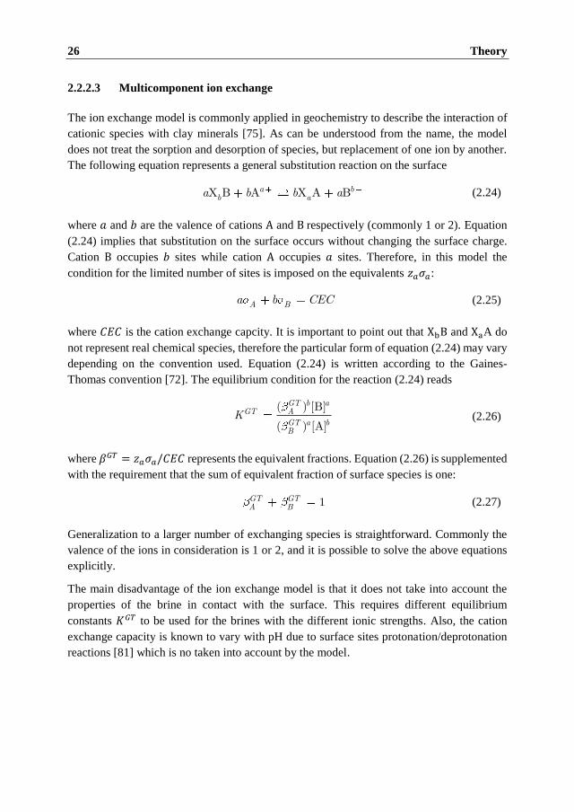
26 Theory

2.2.2.3 Multicomponent ion exchange

The ion exchange model is commonly applied in geochemistry to describe the interaction of

cationic species with clay minerals [75]. As can be understood from the name, the model

does not treat the sorption and desorption of species, but replacement of one ion by another.

The following equation represents a general substitution reaction on the surface

X B A X A Ba bb aa b b a (2.24)

where 𝑎 and 𝑏 are the valence of cations A and B respectively (commonly 1 or 2). Equation

(2.24) implies that substitution on the surface occurs without changing the surface charge.

Cation B occupies 𝑏 sites while cation A occupies 𝑎 sites. Therefore, in this model the

condition for the limited number of sites is imposed on the equivalents 𝑧𝑎𝜎𝑎:

A Ba b CEC (2.25)

where 𝐶𝐸𝐶 is the cation exchange capcity. It is important to point out that XbB and XaA do

not represent real chemical species, therefore the particular form of equation (2.24) may vary

depending on the convention used. Equation (2.24) is written according to the Gaines-

Thomas convention [72]. The equilibrium condition for the reaction (2.24) reads

( ) [B]

( ) [A]

GT b aGT A

GT a bB

K (2.26)

where 𝛽𝐺𝑇 = 𝑧𝑎𝜎𝑎/𝐶𝐸𝐶 represents the equivalent fractions. Equation (2.26) is supplemented

with the requirement that the sum of equivalent fraction of surface species is one:

1GT GTA B (2.27)

Generalization to a larger number of exchanging species is straightforward. Commonly the

valence of the ions in consideration is 1 or 2, and it is possible to solve the above equations

explicitly.

The main disadvantage of the ion exchange model is that it does not take into account the

properties of the brine in contact with the surface. This requires different equilibrium

constants 𝐾𝐺𝑇 to be used for the brines with the different ionic strengths. Also, the cation

exchange capacity is known to vary with pH due to surface sites protonation/deprotonation

reactions [81] which is no taken into account by the model.

2.2 Crude Oil/Brine/Rock Interactions 27

2.2.3 Surface Complexation

The adsorption models described above may be too simplistic to mimic the interaction

between the aqueous solution and the surface. The main disadvantage is that none of them

takes into account the electric state of the surface, which is known to vary considerably with

pH, ionic strength and ionic composition [82]. The application of the above models requires

determining the equilibrium constants for specific conditions, unique for a given combination

of rock and a fluid. A more general approach allowing to overcome these limitations is

introduced by the surface complexation models [79, 80]. These models consider adsorption

on the surface together with the formation of the electric double layer (EDL) [83], which is

briefly introduced below.

At the interface between a charged surface and a solution electric potential is developed. The

theory of double layer [79, 82] refers to two parallel layers surrounding the surface as

illustrated in Figure 2.4. The first layer, known as the Stern layer, is comprised of the ions

that are adsorbed on the surface and are fixed. In this layer, with a typical thickness of 1 nm,

the major part of the potential drop occurs [84]. The second layer, a diffuse layer, has a

thickness between 1 to 500 nm depending on the surface charge and the ionic strength of the

solution. The ions in this layer are attracted to the surface via the Coulomb force. They are

loosely associated with the surface and can move in the fluid under the influence of thermal

motion and electric attraction. The ions with the charge of the opposite sign to those of the

surface are attracted to the surface while the ions with the similar charge are repelled. This

results in the screening of the surface charge. The diffuse layer is split into two separate

regions based on the ability of ions to move (slip) along the surface:

(I) The region between the Stern plane and slipping plane. Ions are not affected by the

tangential stress arising due to the flow of water along the surface.

(II) The region between slipping plane and the bulk fluid. Ions can move under the

influence of tangential stress, meaning the flow of water affects the distribution of

ions in this layer.

Figure 2.4: Illustration of the EDL structure and electric potential for a positively charged surface.

+

+

+

+

+

Stern layerNegatively charged

diffuse layer Bulk fluid

( I ) ( II )

Zeta potential

Stern potential

Surface potential

slipping plane

Stern plane

𝑑

Distance

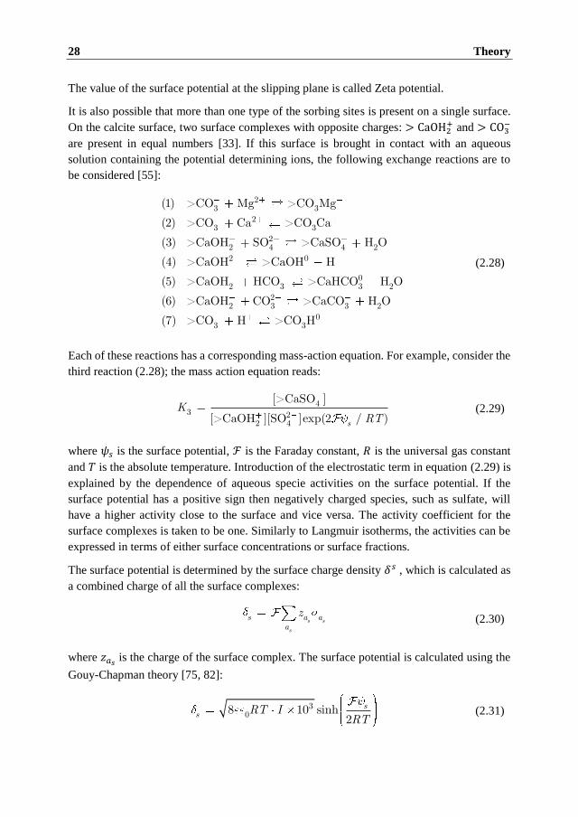
28 Theory

The value of the surface potential at the slipping plane is called Zeta potential.

It is also possible that more than one type of the sorbing sites is present on a single surface.

On the calcite surface, two surface complexes with opposite charges: > CaOH2+ and > CO3

−

are present in equal numbers [33]. If this surface is brought in contact with an aqueous

solution containing the potential determining ions, the following exchange reactions are to

be considered [55]:

23 3

23 3

22 4 4 22 0

02 3 3 2

22 3 3 2

03 3

(1) >CO Mg >CO Mg

(2) >CO Ca >CO Ca

(3) >CaOH SO >CaSO H O

(4) >CaOH >CaOH H

(5) >CaOH HCO >CaHCO H O

(6) >CaOH CO >CaCO H O

(7) >CO H >CO H

(2.28)

Each of these reactions has a corresponding mass-action equation. For example, consider the

third reaction (2.28); the mass action equation reads:

4

3 22 4

[>CaSO ]

[>CaOH ][SO ]exp(2 / )s

KRT

(2.29)

where is the surface potential, ℱ is the Faraday constant, 𝑅 is the universal gas constant

and 𝑇 is the absolute temperature. Introduction of the electrostatic term in equation (2.29) is

explained by the dependence of aqueous specie activities on the surface potential. If the

surface potential has a positive sign then negatively charged species, such as sulfate, will

have a higher activity close to the surface and vice versa. The activity coefficient for the

surface complexes is taken to be one. Similarly to Langmuir isotherms, the activities can be

expressed in terms of either surface concentrations or surface fractions.

The surface potential is determined by the surface charge density 𝛿 , which is calculated as

a combined charge of all the surface complexes:

s s

s

s a aa

z (2.30)

where 𝑧𝑎𝑠 is the charge of the surface complex. The surface potential is calculated using the

Gouy-Chapman theory [75, 82]:

3

08 10 sinh2

ss RT I

RT (2.31)

2.3 The Buckley-Leverett Model 29

where 휀 is the dielectric constant of water, 휀0 is the permittivity of free space and 𝐼 is the

(molal) ionic strength. Equation (2.31) is approximate as it was originally derived for a single

symmetrical electrolyte, rather than for a mixed solution. A more accurate calculation of the

surface potential can be performed with the Grahame equation [82].

The main advantage of the surface complexation model is its ability to account for:

Electrostatic interaction between the aqueous ions and charged surface by

introducing the electrostatic term 𝜒 = exp (ℱ /𝑅𝑇).

Variation of the ionic strength, due to the dependence of surface potential on surface

charge and ionic strength according to the equation (2.31).

Variation of pH due to reactions (4) and (7) in (2.28).

Surface complexation models provide a bridge between the macro-scale surface charging,

sorption properties of carbonate minerals, and the chemical structure of the surface sites.

However, the double layer models suffer from uncertainties and data limitations. Values

reported for the equilibrium constants and site densities can vary over a relatively broad range

[33, 73].

As it was already discussed above, the wetting state of the rock depends on the presence and

stability of the water films that prevent polar compounds in oil to adsorb on the surface. The

stability and properties of the water films are related to the structure of the EDL. Therefore,

surface complexation models can be used to provide a description of the change of the

wetting properties of rocks during the smart water flooding.

2.3 The Buckley-Leverett Model

The Buckley-Leverett model was originally introduced to describe two-phase immiscible

displacement in porous media [85]. It serves as a basis for the development of a mathematical

model for any kind of liquid-liquid displacement in porous media. The original model was

later extended and widely applied for the various types of waterflooding of petroleum

reservoirs, including polymer flooding, carbonated waterflooding, miscible flooding, steam

flooding, and various type of surfactant flooding (see [86] and references therein).

2.3.1 Basics

Consider the flow of immiscible fluids in porous media. The Buckley-Leverett approach is

based on the macroscopic approximation of the mechanics of continuous medium, according

to which fluid phases: water (subscript 𝑤) and oil (𝑜), together with porous matrix, are all

situated at the same macroscopic representative elementary volume (r.e.v.). From the

microscopic point of view, each r.e.v. contains a large number of pores and should in general

be characterized by complex pore geometry and different fluid distributions within it. The

30 Theory

state of each macroscopic point (volume element) is characterized by amounts of each phase,

expressed in volumetric fractions. The volumetric fraction of the space accessible for fluids

is porosity 𝜙, the fractions of the pore space occupied by water and oil are saturations: 𝑠𝑤 =

𝑠 and 𝑠𝑜 = 1 − 𝑠 respectively.

The superficial flow velocities of the phases are introduced as the rates of flow per unit

surface area. The velocities of water and oil are denoted by �� 𝑤 and �� 𝑜 respectively. The total

flow velocity �� 𝑡 is the sum of the phase flow velocities:

t w ou u u (2.32)

The following equations express the mass conservation laws for the phases:

) )( ( 0t w w w wus (2.33)

) )( ( 0t o o o ous (2.34)

where 𝜌𝑤 and 𝜌𝑜 are the densities of water and oil phases, respectively.

2.3.2 Relative Permeabilities

In the macroscopic theory, it is assumed that each phase occupies its own pore system, and

thus the flow of one fluid does not affect another. It may also be interpreted as if the viscous

friction forces act only between the fluid phase and the porous matrix, but not between two

fluid phases. Generalized Darcy laws relate the phase velocities �� 𝑤, �� 𝑜 and the forces driving

the flow of the phasess by means of relative phase permeabilities 𝑘𝑟𝑤(𝑠) and 𝑘𝑟𝑜(𝑠).

( )( )rw

w ww

w

k k su P g (2.35)

( )( )ro

o oo

o

k k su P g (2.36)

where 𝑘 is the absolute permeability, 𝜇𝑤 and 𝜇𝑜 are the oil and water viscosities, 𝑃𝑤 and 𝑃𝑜

are the pressures in the phases and 𝑔 is the gravitational acceleration. The form of equations

(2.35), (2.36) assumes the isotropy of the absolute permeability. In a more general case, the

scalar absolute permeability should be replaced with the permeability tensor 𝐤. It is also

convenient to introduce phase mobilities:

, ,rk w o (2.37)

Using the concept of phase mobilities, equations (2.35), (2.36) assume the form

2.3 The Buckley-Leverett Model 31

),( ,u k P g w o (2.38)

There is no general way to calculate the phase relative permeabilities without conducting

core flood experiments. Moreover, experiments on steady two-phase flow, required for the

direct measurement of phase relative permeabilities, are laborious. In case direct

measurements cannot be carried out, suitable approximations determine the relative

permeability functions. One of the most widely applied models for the relative permeability

functions is the Corey exponent representation [70, 87, 88]:

where 𝑠𝑤𝑖 and 𝑠𝑜𝑟 are the irreducible water saturation and residual oil saturation respectively,

𝑘𝑟𝑜𝑤𝑖 and 𝑘𝑟𝑤𝑜𝑟 are the end point permeabilities and 𝑛𝑤, 𝑛𝑜 are the Corey exponents. These

parameters can be recovered by indirect experimental procedures such as Welge’s or JBN

methods [89, 90], involving certain manipulations with the experimental data from the

flooding experiments. The typical shapes of the relative permeability curves corresponding

to water-wet and oil-wet rocks are shown in Figure 2.5. The rule of thumb for the

characteristic values of Corey parameters for a water-wet system is [91]:

Endpoint saturations: 𝑠𝑜𝑟 around 0.3 and higher; 𝑠𝑤𝑖 around 0.1.

Corey exponents: 𝑛𝑜 around 2 to 3; 𝑛𝑤 around 4 to 6.

End point relative permeabilities: 𝑘𝑟𝑜𝑤𝑖 around 0.6 to 0.8; 𝑘𝑟𝑤𝑜𝑟 around 0.1 to 0.4.

1

wnwi

rw rworwi or

s sk k

s s (2.39)

1

1

onor

ro rowiwi or

s sk k

s s (2.40)

Figure 2.5: Typical oil/water relative permeability curves: (Left) strongly water-wet rock, (Right)

strongly oil-wet rock. Reproduced after Craig [66].

32 Theory

For an oil-wet system, water and oil exchange places. The residual oil saturation of an oil-

wet rock may be very low, however, due to high value of the Corey exponent (𝑛𝑜 around 4

to 6) the relative permeability of oil diminishes quickly with increasing water saturation.

A central concept for the Buckley-Leverett model is the fractional flow function 𝑓𝑤(𝑠) which

is equal to the ratio of the mobility of water to the sum of the mobilities of water and oil:

/

/ /w rw w

ww o rw w ro o

kf

k k (2.41)

The physical meaning of the fractional flow function is the volumetric fraction of water in

the flow.

2.3.3 Transport of Chemicals

The scheme presented above is extended to describe displacement of oil by an aqueous

chemical solution. A chemical substance such as a polymer or a surfactant is added to the

injected water to improve the flooding efficiency. It is usually assumed that concentration of

the chemical is relatively low and does not affect the densities [92].

The material balance equation for transport of the chemical is given by [93]

) )( ( wt w tcuc cs cD (2.42)

where c is the concentration of the chemical in the solution, 𝐃𝑤 is the diffusion/dispersion

tensor, and the term in the right hand side of the equation represents the loss of chemical due

to brine-rock interactions. The asterisk (*) is used to denote the difference between the

aqueous concentrations 𝑐 in mol/l(water) and losses 𝑐∗ in mol/l(core).

2.3.4 Analytical Solutions for Linear Waterflooding

Below we present the original Buckley-Leverett solution, as well as the two important cases

of the chemical flooding. These cases include secondary and tertiary waterflooding, to

illustrate the general features of these classical solutions. The 1D Buckley-Leverett problem

is usually associated with a displacement of oil by water from a horizontal reservoir

developed by parallel lines of injection and production wells. The major assumptions behind

the considered models are [86]:

One dimensional flow in homogeneous, isotropic, isothermal porous medium.

Fluids are incompressible.

Gravity and capillary forces are negligible.

The initial distribution of fluids is uniform.

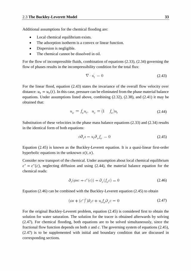
2.3 The Buckley-Leverett Model 33

Additional assumptions for the chemical flooding are:

Local chemical equilibrium exists.

The adsorption isotherm is a convex or linear function.

Dispersion is negligible.

The chemical cannot be dissolved in oil.

For the flow of incompressible fluids, combination of equations (2.33), (2.34) governing the

flow of phases results in the incompressibility condition for the total flux:

0tu (2.43)

For the linear flood, equation (2.43) states the invariance of the overall flow velocity over

distance: 𝑢𝑡 = 𝑢𝑡(𝑡). In this case, pressure can be eliminated from the phase material balance

equations. Under assumptions listed above, combining (2.32), (2.38), and (2.41) it may be

obtained that:

, (1 )w w t o w tu f u u f u (2.44)

Substitution of these velocities in the phase mass balance equations (2.33) and (2.34) results

in the identical form of both equations:

0t t x ws u f (2.45)

Equation (2.45) is known as the Buckley-Leverett equation. It is a quasi-linear first-order

hyperbolic equations in the unknown 𝑠(𝑡, 𝑥).

Consider now transport of the chemical. Under assumption about local chemical equilibrium

𝑐∗ = 𝑐∗(𝑐), neglecting diffusion and using (2.44), the material balance equation for the

chemical reads:

( ( )) ( ) 0t x wsc c c f c (2.46)

Equation (2.46) can be combined with the Buckley-Leverett equation (2.45) to obtain

( ( ) ) 0t t w xs c c u f c (2.47)

For the original Buckley-Leverett problem, equation (2.45) is considered first to obtain the

solution for water saturation. The solution for the tracer is obtained afterwards by solving

(2.47). For chemical flooding, both equations are to be solved simultaneously, since the

fractional flow function depends on both 𝑠 and 𝑐. The governing system of equations (2.45),

(2.47) is to be supplemented with initial and boundary condition that are discussed in

corresponding sections.

34 Theory

The following transformation of variables is conventionally applied to bring the equations

(2.45), (2.47) to dimensionless form

0

1, ( )

t

D D tx

x t u dL L

(2.48)

where 𝑈(𝜏) is the linear velocity corresponding to a given injection rate. The newly defined

time 𝑡𝐷 correspond to the amount of pore volumes injected. Substitution in (2.45), (2.47)

results in the following dimensionless system of equations:

0D Dt x ws f (2.49)

1( ( ) ) 0D Dt w xs c c f c (2.50)

2.3.4.1 The Buckley-Leverett solution

The conventional Buckley-Leverett solution is obtained for the problem of 1D waterflooding,

which is described by a single equation (2.49). The boundary and initial conditions

correspond to the injection of water in porous medium at irreducible water saturation:

(0, ) , ( ,0) 1D wi D ors x s s t s (2.51)

The chemical is assumed not to participate in any interactions, and 0c . Therefore, the

chemical is considered to be a tracer that is present only in the injected water with the molar

concentration 𝑐𝐽. The corresponding initial and boundary conditions assume the form:

(0, ) 0, ( ,0) JD Dc x c t c (2.52)

The Buckley-Leverett solution for the problem (2.49) to (2.52) is shown in Figure 2.6. It

consists of the three main parts [88, 92]:

1. Displacement front (𝑥 = 𝑥𝑤𝑓). Saturation at the displacement front changes

jumpwise from initial water saturation 𝑠𝑤𝑖 to 𝑠𝑓. The position of the displacement

front can be determined from 𝑥𝑤𝑓 = 𝜉𝑓𝑡𝐷 , where 𝜉𝑓 is the front velocity.

2. A region ahead of the displacement front (𝑥 > 𝑥𝑤𝑓). Saturation is equal to the

irreducible water saturation 𝑠 = 𝑠𝑤𝑖 , and only oil is mobile.

3. A region behind the displacement front (𝑥 < 𝑥𝑤𝑓). Both oil and water are mobile.

The saturation is determined according to the following equation [92]:

( ) , /w D Df s x t (2.53)

2.3 The Buckley-Leverett Model 35

The velocity of the displacement front is determined using the Rankine-Hugoniot condition

[94]:

[ ] [[ ][ ] ]fw wf s (2.54)

where ⟦𝑠⟧ = 𝑠+ − 𝑠− represent a jump in the value at the front. In order to determine the

velocity of the displacement front, condition (2.54) is combined with (2.53) to obtain

( )( ) w fw f

f wi

f sf s

s s (2.55)

The above equation allows to determine saturation at the front 𝑠𝑓, which is then used to

calculate the displacement front velocity according to equation (2.54). Equations (2.54) and

(2.55) allow a simple geometric interpretation on the plane of variables (𝑠, 𝑓): velocity of the

displacement front is determined by the tangent line to the fractional flow curve drawn from

the point (𝑠𝑤𝑖; 0) as shown in Figure 2.6b. More generally, a part of the solution

corresponding to a shock is represented by a line on the (𝑠, 𝑓) plane connecting two points

(𝑠0, 𝑓0) and (𝑠1, 𝑓1). The velocity of the corresponding shock is determined by the Rankine-

Hugoniot condition:

0 1

120 1

[ ]]

[ ]

[

[ ]

f f

s s

f

s (2.56)

Figure 2.6: a) Saturation profile for the original Buckley-Leverett solution and concentration

profile for the tracer. b) Fractional flow function.

Injected

water

Connate water

𝑥𝐷

𝑠𝑤

𝑠𝑓

1 − 𝑠𝑜𝑟

𝑥𝑤𝑓

𝑠𝑤𝑖

𝑐𝐽

𝑥𝑐𝑓

𝑐 𝑥𝐷

𝜉𝑓

𝜉𝑐𝑓

𝑠𝑐𝑓

a)

𝑠𝑤𝑖 1 − 𝑠𝑜𝑟

𝑓𝑤

1

𝑠𝑤

(𝑠𝑓; 𝑓𝑤𝑓)

(𝑠𝑐𝑓; 𝑓𝑐𝑓)

b)

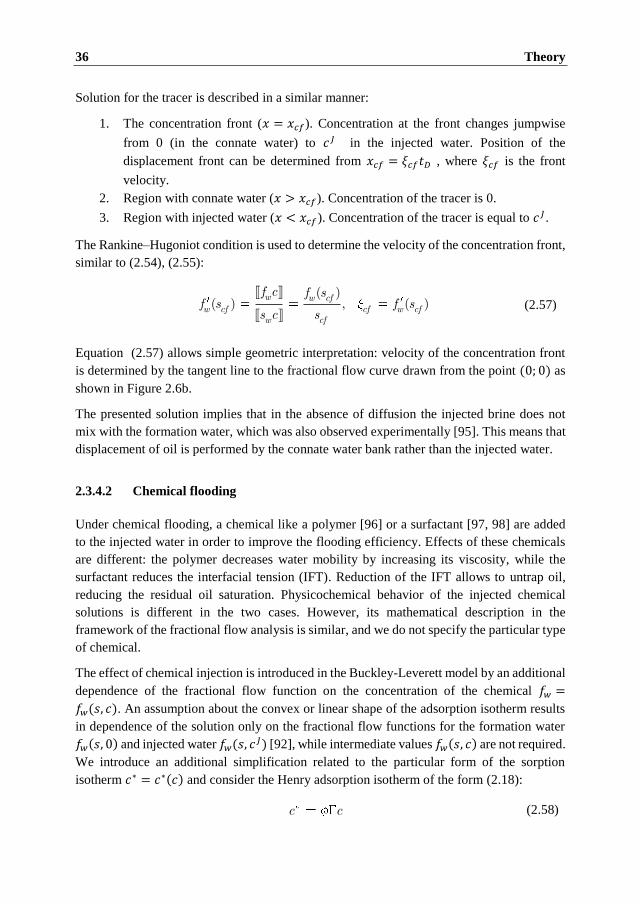
36 Theory

Solution for the tracer is described in a similar manner:

1. The concentration front (𝑥 = 𝑥𝑐𝑓). Concentration at the front changes jumpwise

from 0 (in the connate water) to 𝑐𝐽 in the injected water. Position of the

displacement front can be determined from 𝑥𝑐𝑓 = 𝜉𝑐𝑓𝑡𝐷 , where 𝜉𝑐𝑓 is the front

velocity.

2. Region with connate water (𝑥 > 𝑥𝑐𝑓). Concentration of the tracer is 0.

3. Region with injected water (𝑥 < 𝑥𝑐𝑓). Concentration of the tracer is equal to 𝑐𝐽.

The Rankine–Hugoniot condition is used to determine the velocity of the concentration front,

similar to (2.54), (2.55):

[ ]]

[ ]]

[ ( )( ) , ( )

[ww cf

w cf cfw

w cfcf

f sf s f s

s

f c

s c (2.57)

Equation (2.57) allows simple geometric interpretation: velocity of the concentration front

is determined by the tangent line to the fractional flow curve drawn from the point (0; 0) as

shown in Figure 2.6b.

The presented solution implies that in the absence of diffusion the injected brine does not

mix with the formation water, which was also observed experimentally [95]. This means that

displacement of oil is performed by the connate water bank rather than the injected water.

2.3.4.2 Chemical flooding

Under chemical flooding, a chemical like a polymer [96] or a surfactant [97, 98] are added

to the injected water in order to improve the flooding efficiency. Effects of these chemicals

are different: the polymer decreases water mobility by increasing its viscosity, while the

surfactant reduces the interfacial tension (IFT). Reduction of the IFT allows to untrap oil,

reducing the residual oil saturation. Physicochemical behavior of the injected chemical

solutions is different in the two cases. However, its mathematical description in the

framework of the fractional flow analysis is similar, and we do not specify the particular type

of chemical.

The effect of chemical injection is introduced in the Buckley-Leverett model by an additional

dependence of the fractional flow function on the concentration of the chemical 𝑓𝑤 =

𝑓𝑤(𝑠, 𝑐). An assumption about the convex or linear shape of the adsorption isotherm results

in dependence of the solution only on the fractional flow functions for the formation water

𝑓𝑤(𝑠, 0) and injected water 𝑓𝑤(𝑠, 𝑐𝐽) [92], while intermediate values 𝑓𝑤(𝑠, 𝑐) are not required.

We introduce an additional simplification related to the particular form of the sorption

isotherm 𝑐∗ = 𝑐∗(𝑐) and consider the Henry adsorption isotherm of the form (2.18):

c c (2.58)

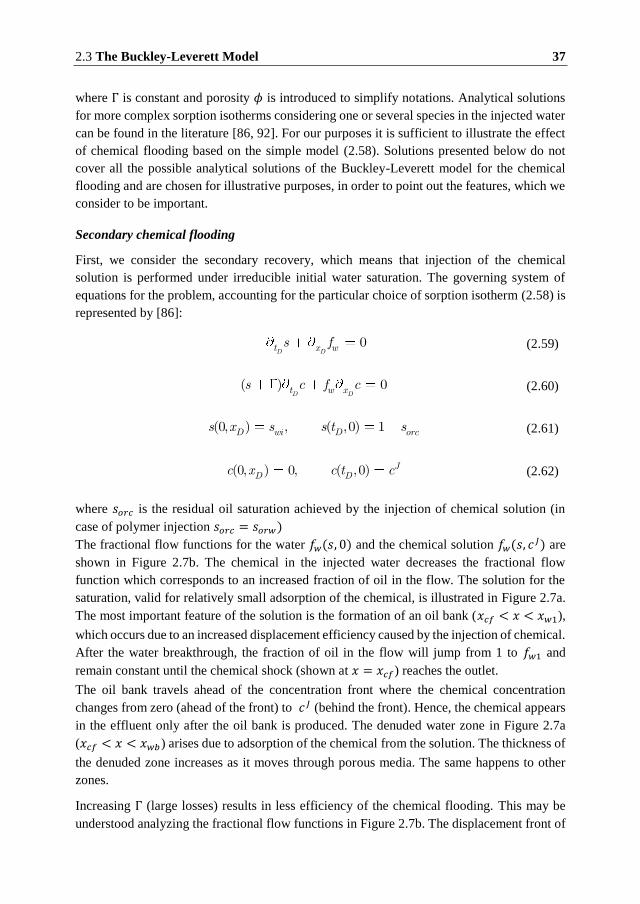
2.3 The Buckley-Leverett Model 37

where Γ is constant and porosity 𝜙 is introduced to simplify notations. Analytical solutions

for more complex sorption isotherms considering one or several species in the injected water

can be found in the literature [86, 92]. For our purposes it is sufficient to illustrate the effect

of chemical flooding based on the simple model (2.58). Solutions presented below do not

cover all the possible analytical solutions of the Buckley-Leverett model for the chemical

flooding and are chosen for illustrative purposes, in order to point out the features, which we

consider to be important.

Secondary chemical flooding

First, we consider the secondary recovery, which means that injection of the chemical

solution is performed under irreducible initial water saturation. The governing system of

equations for the problem, accounting for the particular choice of sorption isotherm (2.58) is

represented by [86]:

0D Dt x ws f (2.59)

( ) 0D Dt w xs c f c (2.60)

(0, ) , ( ,0) 1D wi D orcs x s s t s (2.61)

(0, ) 0 ( ,0), JD Dc x c t c (2.62)

where 𝑠𝑜𝑟𝑐 is the residual oil saturation achieved by the injection of chemical solution (in

case of polymer injection 𝑠𝑜𝑟𝑐 = 𝑠𝑜𝑟𝑤)

The fractional flow functions for the water 𝑓𝑤(𝑠, 0) and the chemical solution 𝑓𝑤(𝑠, 𝑐𝐽) are

shown in Figure 2.7b. The chemical in the injected water decreases the fractional flow

function which corresponds to an increased fraction of oil in the flow. The solution for the

saturation, valid for relatively small adsorption of the chemical, is illustrated in Figure 2.7a.

The most important feature of the solution is the formation of an oil bank (𝑥𝑐𝑓 < 𝑥 < 𝑥𝑤1),

which occurs due to an increased displacement efficiency caused by the injection of chemical.

After the water breakthrough, the fraction of oil in the flow will jump from 1 to 𝑓𝑤1 and

remain constant until the chemical shock (shown at 𝑥 = 𝑥𝑐𝑓) reaches the outlet.

The oil bank travels ahead of the concentration front where the chemical concentration

changes from zero (ahead of the front) to 𝑐𝐽 (behind the front). Hence, the chemical appears

in the effluent only after the oil bank is produced. The denuded water zone in Figure 2.7a

(𝑥𝑐𝑓 < 𝑥 < 𝑥𝑤𝑏) arises due to adsorption of the chemical from the solution. The thickness of

the denuded zone increases as it moves through porous media. The same happens to other

zones.

Increasing Γ (large losses) results in less efficiency of the chemical flooding. This may be

understood analyzing the fractional flow functions in Figure 2.7b. The displacement front of

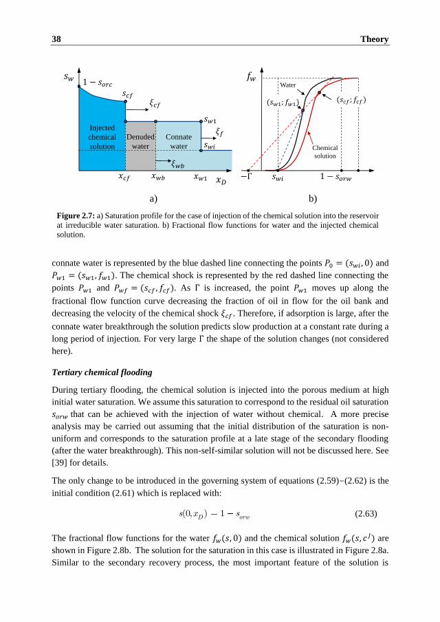
38 Theory

connate water is represented by the blue dashed line connecting the points 𝑃0 = (𝑠𝑤𝑖 , 0) and

𝑃𝑤1 = (𝑠𝑤1, 𝑓𝑤1). The chemical shock is represented by the red dashed line connecting the

points 𝑃𝑤1 and 𝑃𝑤𝑓 = (𝑠𝑐𝑓 , 𝑓𝑐𝑓). As Γ is increased, the point 𝑃𝑤1 moves up along the

fractional flow function curve decreasing the fraction of oil in flow for the oil bank and

decreasing the velocity of the chemical shock 𝜉𝑐𝑓. Therefore, if adsorption is large, after the

connate water breakthrough the solution predicts slow production at a constant rate during a

long period of injection. For very large Γ the shape of the solution changes (not considered

here).

Tertiary chemical flooding

During tertiary flooding, the chemical solution is injected into the porous medium at high

initial water saturation. We assume this saturation to correspond to the residual oil saturation

𝑠𝑜𝑟𝑤 that can be achieved with the injection of water without chemical. A more precise

analysis may be carried out assuming that the initial distribution of the saturation is non-

uniform and corresponds to the saturation profile at a late stage of the secondary flooding

(after the water breakthrough). This non-self-similar solution will not be discussed here. See

[39] for details.

The only change to be introduced in the governing system of equations (2.59)-(2.62) is the

initial condition (2.61) which is replaced with:

(0, ) 1D orws x s (2.63)

The fractional flow functions for the water 𝑓𝑤(𝑠, 0) and the chemical solution 𝑓𝑤(𝑠, 𝑐𝐽) are

shown in Figure 2.8b. The solution for the saturation in this case is illustrated in Figure 2.8a.

Similar to the secondary recovery process, the most important feature of the solution is

Figure 2.7: a) Saturation profile for the case of injection of the chemical solution into the reservoir

at irreducible water saturation. b) Fractional flow functions for water and the injected chemical

solution.

Denuded

water

Injected

chemical

solution

Connate

water

𝑥𝐷

𝑠𝑤

𝑠𝑤1

1 − 𝑠𝑜𝑟𝑐

𝑥𝑤𝑏𝑥𝑐𝑓

𝑠𝑤𝑖

𝜉𝑓

𝜉𝑐𝑓

𝜉𝑤𝑏

𝑠𝑐𝑓

a)

𝑥𝑤1 𝑠𝑤𝑖 1 − 𝑠𝑜𝑟𝑤

𝑓𝑤

b)

(𝑠𝑤1; 𝑓𝑤1)(𝑠𝑐𝑓; 𝑓𝑐𝑓)

−Γ

Chemical

solution

Water

2.4 Conclusions 39

formation of an oil bank (𝑥𝑐𝑓 < 𝑥 < 𝑥𝑤1). This oil bank is formed by the mobilized oil; ahead

of the oil bank (𝑥 > 𝑥𝑤1) oil is immobile. Solution for the concentration of the chemical is

similar to that in the secondary flooding. Adsorption from the solution results in the

occurrence of the denuded zone free of chemical. The oil bank travels ahead of the

concentration front of the chemical.

Increasing Γ results in less efficiency of the chemical flooding. This may be understood by

analyzing the fractional flow curves in Figure 2.8b. As Γ is increased, the point 𝑃𝑤1 =

(𝑠𝑤1, 𝑓𝑤1) moves up along the fractional flow function curve decreasing the fraction of oil in

the flow for the oil bank and decreasing the velocities of the forward and the backward fronts

of the oil bank 𝜉𝑜𝑏 and 𝜉𝑐𝑓 respectively. Therefore, if retention of the chemical in the porous

medium is large, the oil bank is produced after a long period of injection.

2.4 Conclusions

The effect of the smart water flooding is usually related to the change of the wetting state of

the rock. To develop a macroscopic model that can account for the wettability alteration, it

is necessary to relate wettability to the physicochemical processes on the rock surface. This

can be achieved by considering adsorption of potential determining ions. Adsorption of the

ions is expected to change the charge and, hence, the surface potential of the rock. Simple

adsorption models cannot provide an accurate description of the sorption process. The main

reason is that they do not account for the electrostatic interaction between ions in the solution

and the surface. Therefore, more advanced surface complexation models are to be considered.

Figure 2.8: a) Saturation profile for the case of injection of the chemical solution into reservoir at

large initial water saturation 𝑠𝑜𝑟𝑤. b) Fractional flow functions for water and the injected chemical

solution.

Denuded

water

Injected

chemical

solution

Connate

water

𝑥𝐷

𝑠𝑤

𝑠𝑐𝑓

1 − 𝑠𝑜𝑟𝑐

𝑥𝑤𝑏𝑥𝑐𝑓

𝑠𝑤1

1 − 𝑠𝑜𝑟𝑤𝜉𝑐𝑓

𝜉𝑤𝑏

𝜉𝑜𝑏

a)

𝑥𝑤1 −Γ 1 − 𝑠𝑜𝑟𝑤 𝑠𝑤

1 − 𝑠𝑜𝑟𝑐

𝑠𝑤𝑖

𝑓𝑤

b)

(𝑠𝑤1; 𝑓𝑤1) (𝑠𝑐𝑓; 𝑓𝑐𝑓)

Chemical

solution

Water

40 Theory

Change of the wetting state of the rock may affect transport properties of the fluids, resulting

in increased efficiency of the flooding. The macroscopic model for the two-phase flow in

porous media has been described in the literature, and analytical solutions are well known. It

is important to introduce the described surface chemistry in the macroscopic models.

One of the difficulties is that there is no common knowledge of how exactly the transport

properties will change by action of the surface effects, as there is no general way to evaluate

the relative permeability functions. One should be especially careful when considering

tertiary recovery. The extended Buckley-Leverett solution assumes that the ganglia of the

trapped oil join the continuous phase and flow with it when mobilized. It is possible, however,

that other mechanisms govern the flow of oil in this case.

3

3 Numerical Model

In this chapter, we describe the approach that was used to obtain the numerical scheme for

the reactive two-phase flow in porous media. In Section 3.1, we introduce notations and

general formalism based on the conservation laws. In Section 3.2, we explain an approach

used to calculate the spatial differential operators and fluxes. Section 3.3 describes the

integration of the discretized system of equations. The approach used to obtain discretization

scheme of the second order of accuracy is described in the Section 3.4.

3.1 General System of Conservation Laws

We consider a spatial domain Ω ⊂ ℝ3 representing porous medium, which can be a

petroleum reservoir or a core plug. The boundary of the spatial domain is 𝜕Ω ⊂ ℝ3. Latin

indices 𝑖, 𝑗 are reserved to denote the discrete grid cells.

The bulk phases considered are water (subscript w), oil (subscript o) and solid (subscript s).

For a number of problems it is also important to consider surface phases that are indexed with

subscript 𝛼 . The phases are denoted with subscript 𝛼 ∈ {𝑤, 𝑜, 𝑠, 𝛼 }. Chemical species are

indexed with the subscript 𝑎 ∈ Β 𝑝 = {1,… , 𝑛 𝑝}. The subset Β 𝑝𝛼 ⊂ Β 𝑝 represents species

that belong to phase 𝛼. We also use Β 𝑝𝑏𝑢𝑙𝑘 ⊂ Β 𝑝 which is a subset of the indices of the

species in the bulk phases and Β 𝑝 𝑢𝑟𝑓

∈ Β 𝑝 is a subset of the indices of the surface species.

If the two species represent the same chemical substance occurring in different phases it may

be convenient to denote such species with two indexes: {𝑏, 𝛼}, 𝑏 for the chemical substance

and 𝛼 for the phase in which it occurs.

We consider a set of material balance equations in the form

tU F Q S (3.1)

where 𝐔 is the accumulation term, 𝐅 is the flux. The source term 𝐐 in the right hand side of

(3.1) corresponds to injection/production of the phases and species, while the source term 𝐒

corresponds to material transfer due to physicochemical interactions in the system. Variables

introduced in equation (3.1) are explained below.

42 Numerical Model

3.1.1 Accumulation Term

Let 𝑈𝛼 = 𝑈𝛼(𝑡, 𝑥 ), 𝛼 = {𝑤, 𝑜, 𝑠} be the mass concentrations of water, oil and solid phases

per unit volume of the porous medium as functions of time t and position 𝑥 ∈ Ω. According

to this definition:

, , ,U w o s (3.2)

where 𝜌𝛼 is the phase density and 𝛼 is the volumetric fraction of the porous medium

occupied by the phase 𝛼. The volumetric fractions are determined by the porosity and fluid

saturations:

, (1 ), 1o sw s s (3.3)

In a similar manner, we introduce the global concentrations (concentrations per unit volume

of the porous medium) of the chemical species 𝑈𝑎 in the bulk phases:

, , , ,, spa a w oU c as (3.4)

and on the surface:

ˆ ,s

sa a spU A a (3.5)

where 𝑐𝑎 is the molar concentration of species per unit volume of corresponding phase, 𝛼𝑠

is the specific surface area and 𝜎𝑎 is the surface molar concentration.

We now introduce a vector variable 𝐔 representing the accumulation term, such that:

, , , , 1,..., sp

a

Uw o s a n

UU (3.6)

This is not the only possible choice of the accumulation term. Arbitrary linear transformations

may be applied to the system (3.1) resulting in different forms of conservation laws for the

same problem. Such transformations are usually applied to provide a form of conservation

laws convenient for numerical modeling.

3.1.2 Primitive Variables

Variables 𝐔 are associated with the accumulation term. Even though this term identifies the

state of the system, it is not always convenient for calculation of other parameters. The reason

is that most of the closure relations determining densities, relative permeabilities, and rates

of chemical reactions, used in the model, are not described in terms of conservative variables

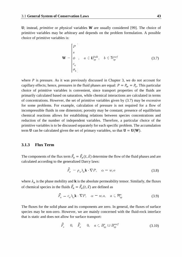
3.1 General System of Conservation Laws 43

𝐔; instead, primitive or physical variables 𝐖 are usually considered [99]. The choice of

primitive variables may be arbitrary and depends on the problem formulation. A possible

choice of primitive variables is:

, ,bulk surfsp p

a

s

b

P

s

a b

c

W (3.7)

where 𝑃 is pressure. As it was previously discussed in Chapter 3, we do not account for

capillary effects; hence, pressures in the fluid phases are equal: 𝑃 = 𝑃𝑤 = 𝑃𝑜. This particular

choice of primitive variables is convenient, since transport properties of the fluids are

primarily calculated based on saturation, while chemical interactions are calculated in terms

of concentrations. However, the set of primitive variables given by (3.7) may be excessive

for some problems. For example, calculation of pressure is not required for a flow of

incompressible fluids in one dimension; porosity may be constant; presence of equilibrium

chemical reactions allows for establishing relations between species concentrations and

reduction of the number of independent variables. Therefore, a particular choice of the

primitive variables is to be discussed separately for each specific problem. The accumulation

term 𝐔 can be calculated given the set of primary variables, so that 𝐔 = 𝐔(𝐖).

3.1.3 Flux Term

The components of the flux term 𝐹 𝛼 = 𝐹 𝛼(𝑡, 𝑥 ) determine the flow of the fluid phases and are

calculated according to the generalized Darcy laws:

, ,oF P wk (3.8)

where 𝜆𝛼 is the phase mobility and 𝐤 is the absolute permeability tensor. Similarly, the fluxes

of chemical species in the fluids 𝐹 𝑎 = 𝐹 𝑎(𝑡, 𝑥 ) are defined as

, , , sa a pP w o aF c k (3.9)

The fluxes for the solid phase and its components are zero. In general, the fluxes of surface

species may be non-zero. However, we are mainly concerned with the fluid-rock interface

that is static and does not allow for surface transport:

0, 0, s surfsp ss a pF F a B B (3.10)

44 Numerical Model

The components of the flux term are calculated based on primitive variables 𝐖. We now

introduce an array of fluxes 𝐅 = 𝐅 (𝐖) such that

, , , , 1,..., spa

Fw o s a n

FF (3.11)

3.1.4 Source Terms

The source term Q arises in the reservoir modeling, where injection and production is

performed through injection and production wells that are located inside the domain Ω. For

the numerical model of a laboratory experiment, the domain Ω is a cylinder representing a

core plug. In this case, injection and production of fluids are performed at the core plug facets

and are expressed by appropriate boundary conditions.

The reactive source term S arises due to physicochemical interactions in the system (e.g.

chemical reactions, sorption). It is responsible for mass transfer between phases and

transformation of species. Similarly to the previously introduced variables, the source term

has the form:

, , , , 1,..., sp

a

Sw o s a n

SS (3.12)

The source term for the phases is related to the chemical species source terms via:

sp

a aa

S M S (3.13)

where 𝑀𝑎 is the molar weight of component. Equation (3.13) states that the change of the

phase mass is due to the change of species concentrations.

The source term for the species 𝑆𝑎 is calculated based on reaction rates and the matrix of

stoichiometric coefficients 𝜈𝑎𝑛, where superscript 𝑛 is used to denote the reaction. For a

system containing 𝑛 𝑝 species undergoing 𝑛𝑟𝑒𝑎𝑐𝑡 reactions, the stoichiometric matrix has the

size of 𝑛𝑟𝑒𝑎𝑐𝑡 × 𝑛 𝑝 and defines reactions according to

1

X 0, 1,...,spn

na a react

a

n n (3.14)

where X𝑎 denotes chemical species. The stoichiometric coefficients are determined in the

following manner: 𝜈𝑎𝑛 > 0 for the products, and 𝜈𝑎

𝑛 < 0 for reactiants. Given the reaction rate

��𝑛 for each of the reactions, the source term 𝑆𝑎 is calculated according to

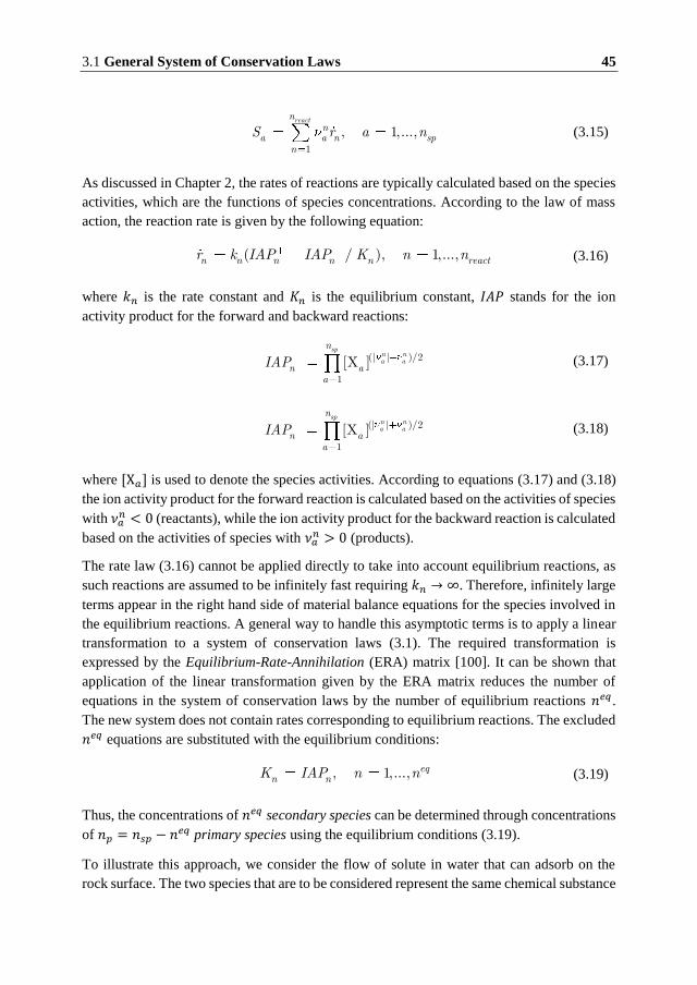
3.1 General System of Conservation Laws 45

1

, 1,...,reactn

na a n sp

n

S r a n (3.15)

As discussed in Chapter 2, the rates of reactions are typically calculated based on the species

activities, which are the functions of species concentrations. According to the law of mass

action, the reaction rate is given by the following equation:

( / ), 1,...,n n n n n reactr k IAP IAP K n n (3.16)

where 𝑘𝑛 is the rate constant and 𝐾𝑛 is the equilibrium constant, 𝐼 𝑃 stands for the ion

activity product for the forward and backward reactions:

(| | )/2

1

[X ]n na a

spn

n aa

IAP (3.17)

(| | )/2

1

[X ]n na a

spn

n aa

IAP (3.18)

where [X𝑎] is used to denote the species activities. According to equations (3.17) and (3.18)

the ion activity product for the forward reaction is calculated based on the activities of species

with 𝜈𝑎𝑛 < 0 (reactants), while the ion activity product for the backward reaction is calculated

based on the activities of species with 𝜈𝑎𝑛 > 0 (products).

The rate law (3.16) cannot be applied directly to take into account equilibrium reactions, as

such reactions are assumed to be infinitely fast requiring 𝑘𝑛 → ∞. Therefore, infinitely large

terms appear in the right hand side of material balance equations for the species involved in

the equilibrium reactions. A general way to handle this asymptotic terms is to apply a linear

transformation to a system of conservation laws (3.1). The required transformation is

expressed by the Equilibrium-Rate-Annihilation (ERA) matrix [100]. It can be shown that

application of the linear transformation given by the ERA matrix reduces the number of

equations in the system of conservation laws by the number of equilibrium reactions 𝑛𝑒𝑞 .

The new system does not contain rates corresponding to equilibrium reactions. The excluded

𝑛𝑒𝑞 equations are substituted with the equilibrium conditions:

, 1,...,neq

nK nAPI n (3.19)

Thus, the concentrations of 𝑛𝑒𝑞 secondary species can be determined through concentrations

of 𝑛𝑝 = 𝑛 𝑝 − 𝑛𝑒𝑞 primary species using the equilibrium conditions (3.19).

To illustrate this approach, we consider the flow of solute in water that can adsorb on the

rock surface. The two species that are to be considered represent the same chemical substance

46 Numerical Model

and, therefore, can be introduced as X1,𝑤 and X1, 𝑢𝑟𝑓 (instead of X1 and X2). According to

(3.14) the adsorption reaction is expressed as

1, 1,X X 0w surf (3.20)

with 𝜈 = [−1; 1] (if no other reactions take place). According to the description introduced

above, the conservation laws for the solute in water and for the surface species in the absence

of convective sources are:

1,1,t w sorw bF rU (3.21)

1,t surf sorbrU (3.22)

The linear transformation matrix, in this case, is E = [1, 1], which corresponds to the

summation of the two equations resulting in

1, 1,1,( 0)t w surf wFU U (3.23)

In terms of primitive variables 𝑐1,𝑤 and 𝜎1, 𝑢𝑟𝑓, the material balance becomes

1, 1, 1,( )ˆ ( ) 0t w ssurf wurf ws A u cc (3.24)

In the case of equilibrium sorption, the material balance for the surface species (3.22) is to

be substituted by the equilibrium condition �� 𝑜𝑟𝑏 = 0. This consideration demonstrates that

in many cases it is easy to determine in which way material balance equations should be

combined in order to eliminate the rates of chemical reactions. For the problems where

species participate in multiple chemical reactions, the general approach that involves the

ERA matrix may be more practical.

A similar transformation can be applied to eliminate the kinetic reaction rates on the right-

hand side of equation (3.1). This transformation does not decrease the order of the governing

system of equations. However, it makes it possible to obtain a form of conservation laws that

can be conveniently solved by the splitting approach introduced in Section 3.3.

3.1.5 Initial and Boundary Conditions

Assuming that all the closure relations required to calculate accumulation term, fluxes and

reactive source term are given, it is only necessary to formulate initial and boundary

conditions to close the system of conservation laws (3.1). The initial conditions are set by an

appropriate choice of primitive variables at the initial time moment 𝐖(0, 𝑥 ). A typical choice

of the initial conditions representing a laboratory water flood experiment is homogeneous

initial saturation, pressure and concentrations of species

3.1 General System of Conservation Laws 47

(0)(0, )xW W (3.25)

The boundary conditions are specified at the boundary 𝜕Ω. For a laboratory flood domain Ω

has a cylindrical shape, such that one facet corresponds to the injection surface (inlet) 𝜕Ω𝑖𝑛 ,

while another corresponds to the production surface (outlet) 𝜕Ω𝑜𝑢𝑡 . The side surface 𝜕Ω𝑛𝑓 is

impermeable. The boundary conditions at the inlet and the side surface read

( ( )) /in

iin

njn t A xF q (3.26)

nfxF 0 (3.27)

where �� is the outward normal vector to the surface 𝜕Ω𝑖𝑛 and 𝐪𝑖𝑛𝑗 = [𝐪𝛼 , 𝐪𝑎]𝑇 is the

specified injection rate with the following components:

, , ,

0,

, ,

0,

, ,

,

inj

sinj inj

spas surf

a sp sp

a

q q w o

q

q c q w o a

q B Ba

(3.28)

𝑞𝛼𝑖𝑛𝑗= 𝑞𝛼

𝑖𝑛𝑗(𝑡) is the variable volumetric injection rate of fluids, and 𝑐𝑎

𝑖𝑛𝑗= 𝑐𝑎

𝑖𝑛𝑗(𝑡) is the

injected fluid composition.

The boundary condition at the outlet 𝜕Ω𝑜𝑢𝑡 is usually given by the outlet pressure:

( , ) ( )out outP t x P t x (3.29)

This is sufficient to calculate the outgoing flux and to close the system (3.1), (3.25), (3.26),

(3.27), provided that all necessary closure relations are given.

3.1.6 Pressure Equation

A general form of the pressure equation is obtained by combining the material balance

equations for the bulk phases

1 1 1 1t FU Q S (3.30)

Taking into account (3.2) and volumetric constraint 1 one obtains

48 Numerical Model

1 1 1 1t Q SF (3.31)

In many applications (like immiscible flooding by a compressible fluid), the fluid density is

considered to be a function of pressure only. Therefore, equation (3.31) contains only

pressure under the time derivative, which explains the reason to call it the pressure equation

and to consider separately. In the cases where density also depends on fluid composition 𝑐𝑎,

the time derivative of concentration will arise on the left-hand side of the equation. This will

affect the choice of the solution scheme, as discussed later.

Another feature of equation (3.31) is that the last term on the right-hand side ∑ 𝜌𝛼−1𝑆𝛼𝛼 may

be non-zero. The combined mass of the phases cannot change due to reactions between them

(assuming that the surface mass transfer is negligible) and ∑ 𝑆𝛼𝛼 = 0. However, ∑ 𝜌𝛼−1𝑆𝛼𝛼

is not equal to zero, which means that there is no volumetric balance associated with the

interphase mass transfer. Therefore, a considerable mass transfer is expected to have an effect

on pressure in the system.

3.2 Spatial Discretization

Below we describe the numerical representation of the spatial derivative operators in the

general system of conservation laws (3.1). Different approaches may be used for this purpose.

Most of them are variations and combinations of the three basic methods: the finite difference

method (FDM), the finite volume method (FVM) and the finite element method (FEM) [101-

103].

In our work FVM has been chosen for the spatial discretization. It is based on the control

volume formulation. This method is extensively used in fluid mechanics, heat and mass

transfer, and the associated problems of chemical and petroleum engineering [102]. The FVM

can be applied for arbitrary geometries and both structured and unstructured grids. A physical

domain is represented as an union of smaller domains called control volumes. The solution

is approximated on an element by the cell average at the center of each element. The flux

term is reduced to a surface integral by using the divergence theorem, which results in the

conservative scheme. Computation of the boundary fluxes is usually performed using the

two-point flux approximation (TPFA) [104], which is of the first order of accuracy in space.

Higher order schemes based on multi-point flux approximations (MPFA) are not easy to

obtain in the case of complex geometries; additionally, they also experience stability issues

in cases where shocks are present in the solutions. One of the possibilities to overcome this

difficulty is to use the flux limiters [99, 101]. The main idea behind this approach is to use

linear piece-wise approximations of variables at the cell boundaries. In this approach, the

accuracy of discretization degrades to the first order in the neighborhood of the shock but

tends to the second order over smooth parts of the solution.

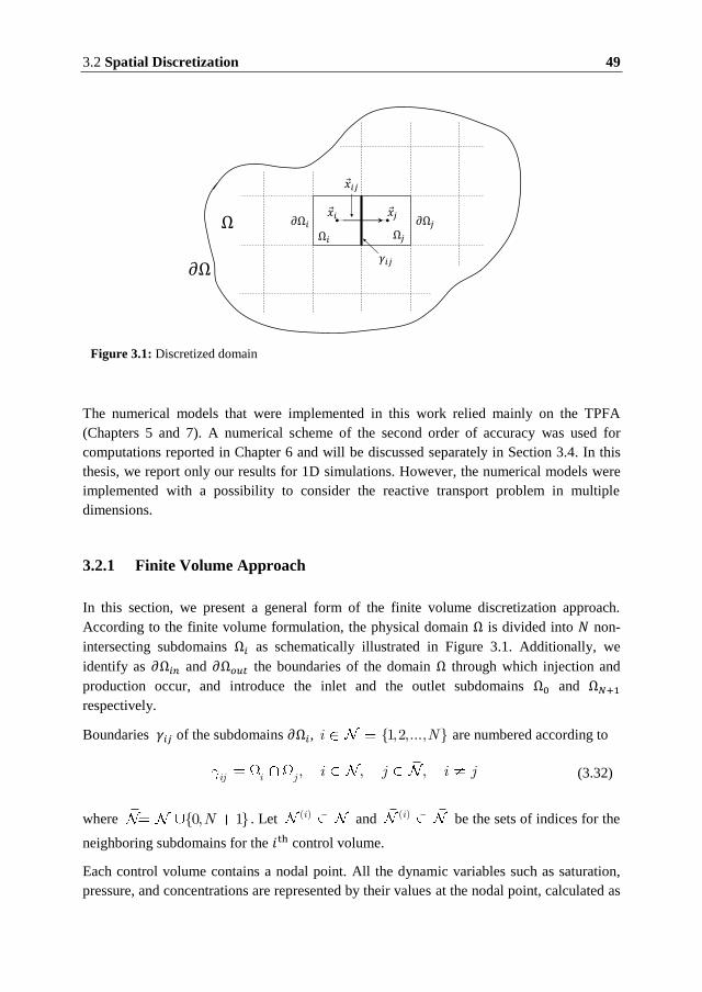
3.2 Spatial Discretization 49

The numerical models that were implemented in this work relied mainly on the TPFA

(Chapters 5 and 7). A numerical scheme of the second order of accuracy was used for

computations reported in Chapter 6 and will be discussed separately in Section 3.4. In this

thesis, we report only our results for 1D simulations. However, the numerical models were

implemented with a possibility to consider the reactive transport problem in multiple

dimensions.

3.2.1 Finite Volume Approach

In this section, we present a general form of the finite volume discretization approach.

According to the finite volume formulation, the physical domain Ω is divided into 𝑁 non-

intersecting subdomains Ω𝑖 as schematically illustrated in Figure 3.1. Additionally, we

identify as 𝜕Ω𝑖𝑛 and 𝜕Ω𝑜𝑢𝑡 the boundaries of the domain Ω through which injection and

production occur, and introduce the inlet and the outlet subdomains Ω0 and Ω𝑁+1

respectively.

Boundaries 𝛾𝑖𝑗 of the subdomains 𝜕Ω𝑖, {1,2,..., }i N are numbered according to

, ,,ij i j i j i j (3.32)

where {0, 1}N . Let ( )i and ( )i be the sets of indices for the

neighboring subdomains for the 𝑖th control volume.

Each control volume contains a nodal point. All the dynamic variables such as saturation,

pressure, and concentrations are represented by their values at the nodal point, calculated as

Figure 3.1: Discretized domain

Ω𝑖 Ω𝑗

𝛾𝑖𝑗

𝜕Ω𝑖𝑥 𝑖 𝑥 𝑗

𝜕Ω𝑗

𝑥 𝑖𝑗

Ω

𝜕Ω

50 Numerical Model

the averages over the corresponding control volume. The location of the 𝑖th control volume

is denoted by 𝑥 𝑖, and we define the internode connection vector

( ), , ,| |iji

ij i j ijx ix x x x j (3.33)

For all the discretized variables used below, designation 𝑢𝑖 means that the value of 𝑢 is

evaluated at the nodal point 𝑥 𝑖 , while 𝑢𝑖𝑗 means that this value is evaluated at the interface

𝛾𝑖𝑗. The volume of the 𝑖th control element is denoted by 𝑉𝑖 .

Consider a general advection-reaction equation (3.1). The discretized equation is obtained by

performing integration of (3.1) over the control volume Ω𝑖

( ) ,i i i

t dV dV idVU Q SF (3.34)

The volume integral of the accumulation term is discretized using the average value of 𝐔

over the control volume:

( ) ,i

idV V iU U (3.35)

Similarly, the volume integral of the source terms on the right-hand side is substituted by

( ) (( ) ) ,i

idV V iQ S Q S (3.36)

The volume integral of the convective flux divergence is transformed into surface integral

using the Gauss’ divergence theorem:

( )

,i iii j

i ij

n dS n dS iF FF (3.37)

where �� 𝑖 is the outward normal vector to the subdomain boundary 𝜕Ω𝑖. An approximation of

the integral over the cell boundary 𝛾𝑖𝑗 is obtained using the midpoint rule:

( )( ) , ,iji ij

in dS n A i jF F (3.38)

where �� 𝑖𝑗 is the normal vector of interface 𝛾𝑖𝑗, 𝐅 𝑖𝑗 is the flux across interface, and 𝑖𝑗 is the

interface area. Substitution of the discrete representations of the volume integrals (3.35),

(3.36) and (3.38) into (3.34) gives the discrete system of conservation laws in the form:

( )

( ) ( )i

di i ij i i idt

j

V n A V iU F Q S (3.39)

3.2 Spatial Discretization 51

For the phase mass transport and transport of the chemical species, the fluxes between two

subdomains are given by the following expressions:

,

( )(( ) ) , , , ,ij iii

jj u P i j w oF k (3.40)

( ), ( ) ) , , ; , ;( i

a ij ia spa ij jc u P i j o ac wF k (3.41)

Due to apparent similarity of equations (3.40) and (3.41), we perform transformations only

with the phase flux while the result for the flux of chemical species is obtained by analogy.

Substitution of (3.40) into (3.38) yields

( )( ) ( ) ( ) , ,ij ij ii

j ij ijP in A n A jF k (3.42)

For the TPFA a first order approximation of the pressure gradient ijP is used:

( ), , i

ij ijij ij

P x PP e i j

x x x (3.43)

Where Δ𝑃𝑖𝑗 = 𝑃𝑗 − 𝑃𝑖 , 𝑒 𝑖𝑗 = 𝑥 𝑖𝑗/Δ𝑥𝑖𝑗 is the unit vector along the internode connection.

Substitution of (3.43) in (3.42) yields

( )( ) ( ) , ,ij ij ij ij ij

ij

iPA

e inx

jn Ak

F (3.44)

The transmissibility is usually introduced according to [105, 106]

),

( )

(

( ) ,

0,

i

i

ijijij

An e j

x i

j

k (3.45)

Transmissibilities for the component fluxes are obtained by substituting 𝜌𝛼 with 𝑐𝑎 in

equation (3.45). More details are given in the next subsection.

Using the transmissibility one may write

( )

( )) (i

ij ijjj

n A iPF (3.46)

For the subdomains in contact with the inlet and outlet subdomains equation (3.39) contains

additional terms corresponding to the flux through the external boundary 𝜕Ω. According to

the formulated boundary conditions, injection flux is specified at the inlet according to (3.26)

, and pressure is specified at the outlet according to (3.29). The external boundary fluxes are

then calculated as follows

52 Numerical Model

,0

(,

00

)( ) ,i

inji in dS n A iF F (3.47)

, 1,

( 1)1( ) ,

i Ni

Ni Nn dS iPF (3.48)

where 𝑃𝑁+1 = 𝑃𝑜𝑢𝑡.

To simplify the notations we define

0

(0)

( 1),

, 1

( ) ,

( ) ( ) ,

0, otherwise

inji

BCi i N

N

n A i

V P i

F

Q (3.49)

Substituting relations (3.46) and (3.49) in the discrete system of conservation laws (3.39)

yields

( ) ( ) ,BCdi i ij i i i idt

j

V P V iU Q Q S (3.50)

The discrete formulation of the system of conservation laws makes it possible to account for

the boundary conditions by introducing an additional source term 𝐐𝑖𝐵𝐶 defined according to

equation (3.49). The form of conservation laws represented by equation (3.39) is more

general than those given by equation (3.50) as, in general, different approaches may be used

to calculate boundary fluxes.

3.2.2 Calculation of Transmissibilities

A common approach to calculate transmissibility is to consider it as a product of the

geometric and the fluid parts [105]. The first term in the brackets in equation (3.45) represents

the geometric part Γ𝑖𝑗 which depends only on reservoir properties and the grid:

( ),,ii

jij

An e i j

xk (3.51)

The fluid part 𝐻𝛼,𝑖𝑗 is determined by the fluid density 𝜌𝛼 and mobility 𝜆𝛼

( ), ( ) , ,ij i

ijH ji (3.52)

Calculation of the geometric part of the transmissibility is not straightforward for a

heterogeneous porous medium in the case of arbitrary grid geometry, especially if the cell

boundaries are not coincident [107]. In this work we apply the Cartesian grids and the

3.2 Spatial Discretization 53

diagonal permeability tensor 𝐤 = 𝑑𝑖𝑎𝑔(𝑘𝑥𝑥 , 𝑘𝑦𝑦, 𝑘𝑧𝑧). For the Cartesian grid, the normal

vector at the cell interface is codirected with the internode vector 𝑒 𝑖𝑗 = �� 𝑖𝑗. Therefore, the

product �� ∙ 𝐤 ∙ 𝑒 is equal to 𝑘𝑥𝑥, 𝑘𝑦𝑦 or 𝑘𝑧𝑧 depending on the location of a neighboring cell.

A subdomain with a lower permeability controls the flow between the adjacent subdomains,

and the transmissibility is calculated as a harmonic average [106]. For example, if 𝑖 and 𝑗 are

the neighbors in 𝑥 direction, calculation of the geometric part Γ𝑖𝑗 is performed according to

( ), i

ij xxij

jA

k ix

(3.53)

, ,

( )/ /

ijxx ij

i xx i j xx j

xk

x k x k (3.54)

where Δ𝑥𝑖 is the distance between the nodal center 𝑥 𝑖 and the boundary 𝛾𝑖𝑗, so that Δ𝑥𝑖𝑗 =

Δ𝑥𝑖 + Δ𝑥𝑗. In the case of uniform grid spacing such that Δ𝑥𝑖 = Δ𝑥𝑗, ∀𝑖, 𝑗 , the average (3.54)

becomes

( ) ( )( )

( ) ( )xx i xx j

xx ijxx i xx j

k kk

k k (3.55)

For the calculation of the geometric part at an interface between the domain and the outlet

Γ𝑖,𝑁+1, it is assumed that the flow is determined only by permeability inside the domain and

that 𝐤𝑖,𝑁+1 = 𝐤𝑖.

The fluid part of transmissibility is calculated using the single point upwind (SPU) scheme

[101]. In the absence of gravity, diffusion, and capillary pressure difference, the direction of

flow at the interface is determined only by the pressure difference:

,

( )( ) 0

( ),

0i ij

ijj ij

iP

PjH i (3.56)

One of the reasons to split the transmissibility into the geometric and fluid parts is that for

inert porous medium, where porosity and absolute permeability are constant, calculation of

the geometric part is performed once at the initialization step. For the simulations where

properties of porous medium vary with time, calculation of both geometric and fluid parts is

performed at each time instant.

54 Numerical Model

3.3 Solution Procedure

A proper method should be chosen in order to solve the discrete system of conservation laws

for the reactive transport described by system (3.39). There are essentially two different

approaches that might be used. The first approach is to preserve coupling between advection

and reaction terms, which means no modifications to be introduced in the system of the

conservation laws. This approach was used for our computations presented in Chapter 4,

where equations were strongly coupled. Another approach is to split the system (3.39) into

the pure advection problem, where only convective terms are considered, and the source

problem, where only reactive source terms are considered [99]. A main advantage of splitting

is that independent methods may be applied to solve each of the subproblems separately. The

computations performed in Chapters 6 and 7 were based on the splitting approach.

Equation (3.39) can be rewritten in the following form:

( , ) ( ) ( , ), ,advectdi i j i j i jdt

t t i jU f W S W f W (3.57)

( )

1 ( ) ,i

advecti i ij i

j

V n A if F Q (3.58)

where 𝐟𝑖𝑎𝑑𝑣𝑒𝑐𝑡 is the convective term that combines the surface fluxes and the convective

sources. According to the coupling approach, the solution is obtained by integrating the full

system of equations (3.57). Splitting of the problem (3.57) is performed in the following way.

For each time interval 𝑡 ∈ [𝑡𝑛, 𝑡𝑛+1], the solution of the problem is obtained by the successive

integration of the following advection problem

1, , ][ ,,adv n nectd

i idti t ttU f (3.59)

and the source problem

1,, [ , ]n ndi idt

ti ttU S (3.60)

Each of the equations (3.57), (3.59), (3.60) represents a system of ordinary differential

equations which can be solved using common integration techniques. In our work, we make

use of explicit and implicit Euler methods. A particular integration scheme may vary

depending on, what variables 𝐖 are treated implicitly and what are treated explicitly. The

commonly applied approaches are [108]: the fully explicit method; implicit pressure, explicit

saturations and explicit compositions (IMPESC) method; the fully implicit method (FIM).

These approaches are explained below.

3.3 Solution Procedure 55

3.3.1 Temporal Integration

In our computations, we used explicit and implicit Euler methods to carry out the time

integration of the ordinary differential equations representing the conservation laws. Both

methods are first order accurate in time. The forward (or explicit) Euler method can be

numerically unstable, especially in the case of stiff equations, which may result in unlimited

growth of the numerical solution and oscillatory behavior [109].

Consider an ordinary differential equation for a vector variable 𝐰 of the form

( ) ( , )ddt

tu w f w (3.61)

Variable 𝐰 may represent the cell average values of a single primitive variable 𝑊 or of a set

of primitive variables. We assume that 𝐰 has 𝑚 components, the same number as the vector

functions 𝐮: ℝ𝑚 → ℝ𝑚 and 𝐟: ℝ𝑚 → ℝ𝑚. Integration of equation (3.61) over time between

the time instants 𝑡 = 𝑡𝑛 and 𝑡 = 𝑡𝑛+1 = 𝑡𝑛 + Δ𝑡 results in

1

1 ( ( ), )n

n

tn n

tt t dtu u f w (3.62)

where 𝐮𝑛 = 𝐮(𝐰𝑛), 𝐰𝑛 = 𝐰(𝑡𝑛).

3.3.1.1 Explicit Euler method

According to the forward, or the explicit Euler method, calculation of the time integral on the

right-hand side of equation (3.62) is performed using the value of the vector function 𝐟 at a

time instant 𝑡 = 𝑡𝑛:

1 ( , )n n n nt tu u f w (3.63)

The value of the primitive variable 𝐰 at the time instant 𝑡 = 𝑡𝑛+1 can then be determined

from the set of algebraic equations

1 1( )n nu w u (3.64)

The forward Euler method should be applied with precautions. In the cases where the right-

hand side of equation (3.63) is large, the value of 𝐮𝑛+1 may change significantly and go

beyond the physical limits. In order to prevent this behavior, it is required to decrease the

time step Δ𝑡. This may limit the application of the explicit Euler method, as it becomes

computationally ineffective if the time step is too small.

56 Numerical Model

3.3.1.2 Implicit Euler method

According to the backward, or the implicit Euler method, calculation of the time integral on

the right hand side of equation (3.62) is performed using the value of the vector function 𝐟 at

a time instant 𝑡 = 𝑡𝑛+1:

1 1 1( ) ( , )n n n nt tu w u f w (3.65)

In general, (3.65) represents a system of non-linear algebraic equations for the variable 𝐰𝑛+1.

Solution for the system (3.65) can be obtained using an iterative procedure. In our

computations presented in Chapter 4 we implemented the multivariate Newton’s method

[110] to solve the governing system of equations that had the form of (3.65) (see description

in the next subsection). A main advantage of the implicit Euler method is its stability.

However, it is characterized by high numerical diffusion [109]. For this reason, even for fine

grids the resulting solution does not reproduce sharp saturation and concentration fronts.

Multivariate Newton method

The multivariate Newton method is a generalization of the Newton-Raphson method onto

multiple dimensions. In order to solve system (3.65), the residual function 𝐠: ℝ𝑚 → ℝ𝑚 is

introduced:

1( ) ( ) ( , ) 0n nt tw u w u wg f (3.66)

The solution of the system (3.66) is obtained recursively. In our computations, the seed value

𝐰[0] was given by 𝐰𝑛 which is the value of variable at the time instant 𝑡 = 𝑡𝑛. The solution

approximation 𝐰[𝑘+1] at iteration 𝑘 is obtained using

[ 1] [ ] 1 [ ]( )k k kg ww w J (3.67)

The iterations are repeated until the convergence criterion ‖𝐰[𝑘+1] −𝐰[𝑘]‖ < 휀𝑡𝑜𝑡 is

fulfilled. The Jacobian matrix J of function 𝐠(𝐰) is defined as

( )( ) , , 1,...,

kll

kgJ k l mw

ww (3.68)

Calculation of the Jacobian J can be performed numerically. This is time costly, but allows

more flexibility, so that numerical method can be applied to different problems without

modification. Computation of the numeric Jacobian is performed according to

( ) ( )( ) k l

ll

kk

ggJ

w e ww (3.69)

3.3 Solution Procedure 57

where 𝐞𝑙 is the vector that introduces a small perturbation of the variables 𝐰 such that the 𝑙th

component of 𝐞𝑙 equal to 𝜖𝑙 and the rest are zero.

3.3.1.3 IMPESC method

The IMPES (and IMPESC) method is motivated by the observation that pressure waves travel

much faster than saturation or concentration waves. The equation governing the evolution of

pressure is elliptic or parabolic, and pressure propagates almost instantaneously through the

domain. In the limiting case of incompressible fluids, the pressure wave travels with infinite

velocity. Equations governing transport of fluids and species are hyperbolic, and

corresponding saturation and concentration waves travel with finite velocities.

According to the IMPESC method, saturation and compositions are considered constant

within the time step. Under this assumption, the material balance equations for the bulk

phases are combined to obtain the pressure equation (3.30) that is used to compute pressure

implicitly. The solution for the pressure is then used to calculate fluxes and perform an

explicit update of the saturation and species concentrations.

3.3.2 Coupling Approach

In this section, we consider the coupling approach that was used for computations in Chapter

4. The system of discretized equations for the coupled reactive transport is given by (3.57).

Simulations of the flow of compressible fluids in porous media, which properties vary in time

and space, were performed in one dimension. The densities of the phases were considered to

be functions of pressure and composition. Additionally, the compositions of the phases were

affected by the undergoing chemical kinetic reactions with sufficiently high reaction rates.

The best performance was achieved using the FIM.

Integration of the system (3.57) was performed using the backward Euler method, so that all

the physical variables: pressure, saturation and compositions were updated implicitly. The

matrix variable 𝐖𝑖 of the size 𝑛𝐖 × 𝑁 (𝑁 is the number of grid cells and 𝑛𝐖 is the number

of primitive variables) was transformed into the vector variable 𝐰 with 𝑚 = 𝑛𝐖 ∙

𝑁 components by reordering:

{( 1) 1,..., } , 1,...,ii n i n i NW Ww W (3.70)

The same applies to the matrix functions 𝐔𝑖 and 𝐟𝑖. As a result, the matrix equation (3.57) is

transformed into a vector equation that has the form of (3.65) and is solved using the

multivariate Newton’s iterations.

The size of the Jacobian J is 𝑚2 = 𝑛𝐖2 ∙ 𝑁2. Most of the computations are performed during

Newton’s iterations, in order to calculate the inverse of the Jacobian. This limits direct

58 Numerical Model

application of the backward Euler method in the case of a large number of variables and fine

grids.

3.3.3 Splitting Approach

A motivation behind splitting, represented by equations (3.59), (3.60), is a possibility for

optimal application of the developed integration schemes for each of the subproblems.

Consider the reaction-advection problem on a time interval 𝑡 ∈ [𝑡𝑛, 𝑡𝑛+1]. The sequential

approach can be illustrated as follows. First, a pure advection problem is considered and an

intermediate solution ��𝑖𝑛 is obtained:

1( )

( )

( ) ( )advectdi n n

ij i jdt

in ni i

tt

W WW W

U W f W (3.71)

The initial condition for the advection problem is given by the values of primitive variables

at the time instant 𝑡 = 𝑡𝑛. The numerical solution for the advection problem is commonly

obtained using the FIM, IMPESC or the fully explicit method. The fully explicit method can

only be applied if calculation of the pressure is not required: for example, in the case of flow

of incompressible fluids in one dimension.

As a second step, the source problem is considered and the solution 𝐖𝑛+1 is obtained:

1

( )

( ) ( )nin n

di j i jdt

i it

U WW

S

W

W

W (3.72)

The intermediate solution ��𝑖𝑛 for the advection problem is used as the new initial condition

for problem (3.72). Computation of the reaction step represented by (3.72) can be performed

using the explicit or the implicit method. The choice depends on the intensity of

physicochemical interactions. For reactions characterized by slow reaction rates, the explicit

method can be used, while for fast reactions one should choose the implicit method. In our

computations, we have used the implicit method by means of Matlab® fsolve function

(Chapter 6) and a solver from the Fortran minpack library [111] (Chapter 7).

A main drawback of the splitting approach is that even though it is possible to construct high

order schemes, the method does not guarantee convergence to the exact solution [99].

However, the benefits of the methods prevail, so that it is widely applied in the reactive

transport modeling.

3.4 Shock Capturing Numerical Scheme 59

3.4 Shock Capturing Numerical Scheme

In this section, we describe the second order accurate scheme that was used for the numerical

modeling in Chapter 6. Below we consider for demonstration the flow of the incompressible

fluids in one dimension.

3.4.1 Flow in One Dimension

The two-phase flow in one dimension represents a special case of the formalism introduced

in Section 3.2. Each subdomain (cell) Ω𝑖 is connected to the two neighboring cells Ω𝑖−1 and

Ω𝑖+1. Injection is performed into cell Ω1 and production occurs from cell Ω𝑁. We assume

that all the cell boundaries are coincident and 𝑖𝑗 = 𝑐𝑜𝑛𝑠𝑡. In the 1D case it is convenient to

denote the boundary values 𝑢𝑖,𝑖±1 as 𝑢𝑖±1/2. The advection-reaction problem reads:

( ) ( )t xU W FW S (3.73)

Discretized system of conservation laws (3.39) assumes the form

1/2 1/2

,i ii

ii

di

dt x

F FUS (3.74)

where 𝐅1/2 is the external flux to the first cell, and 𝐅𝑁+1/2 is the outgoing flux from the last

cell. For the flow of incompressible fluids in one dimension, the linear flow velocity 𝑢𝑡 is

constant and phase velocities are determined in terms of the fractional flow function:

t a a tu f u u c f u (3.75)

Pressure can be eliminated from the set primitive variables and 𝐖 = [𝑠, 𝑐𝑎, 𝜎𝑏]𝑇 , 𝑎 ∈ Β 𝑝

𝑤 ,

𝑏 ∈ Β 𝑝 𝑢𝑟𝑓

.

3.4.2 MUSCL-Hancock Scheme

Construction of the high-order accurate schemes for the conservation laws is a subject of

numerous books and publications [99, 101] and we cannot fully cover its application.

Therefore, we briefly introduce the numerical technique applied in this work without going

deeply into details. It is required to split the reactive transport model represented by (3.73)

into pure advection problem:

( ) ( ) 0t xU W FW (3.76)

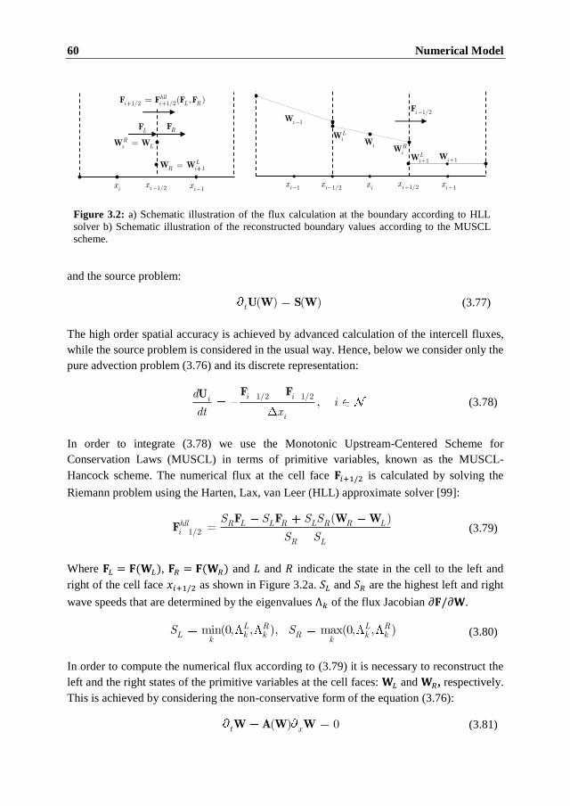
60 Numerical Model

and the source problem:

( ) ( )tU W S W (3.77)

The high order spatial accuracy is achieved by advanced calculation of the intercell fluxes,

while the source problem is considered in the usual way. Hence, below we consider only the

pure advection problem (3.76) and its discrete representation:

1/2 1/2

,i ii

i

di

dt x

F FU (3.78)

In order to integrate (3.78) we use the Monotonic Upstream-Centered Scheme for

Conservation Laws (MUSCL) in terms of primitive variables, known as the MUSCL-

Hancock scheme. The numerical flux at the cell face 𝐅𝑖+1/2 is calculated by solving the

Riemann problem using the Harten, Lax, van Leer (HLL) approximate solver [99]:

1/2

( )R L L R L R R Lhlli

R L

S S S S

S S

F F W WF (3.79)

Where 𝐅𝐿 = 𝐅(𝐖𝐿), 𝐅𝑅 = 𝐅(𝐖𝑅) and 𝐿 and 𝑅 indicate the state in the cell to the left and

right of the cell face 𝑥𝑖+1/2 as shown in Figure 3.2a. 𝑆𝐿 and 𝑆𝑅 are the highest left and right

wave speeds that are determined by the eigenvalues Λ𝑘 of the flux Jacobian 𝜕𝐅/𝜕𝐖.

min(0, , ), max(0, , )L R L RL k k R k k

k kS S (3.80)

In order to compute the numerical flux according to (3.79) it is necessary to reconstruct the

left and the right states of the primitive variables at the cell faces: 𝐖𝐿 and 𝐖𝑅, respectively.

This is achieved by considering the non-conservative form of the equation (3.76):

( ) 0t xW AW W (3.81)

Figure 3.2: a) Schematic illustration of the flux calculation at the boundary according to HLL

solver b) Schematic illustration of the reconstructed boundary values according to the MUSCL

scheme.

ix

Ri LW W

1L

R iW W

RFLF

1/2 1/2( , )hlli i L RF F F F

1ix1/2ix ix

iWLiW

RiW

1LiW 1iW

1iW1/2iF

1ix 1/2ix 1/2ix 1ix

3.4 Shock Capturing Numerical Scheme 61

where 𝐀(𝐖) = (∂𝐔/ ∂𝐖)−𝟏(∂𝐅/ ∂𝐖). Computation of 𝐖𝐿 and 𝐖𝑅 is performed in two

steps:

Step I: Data reconstruction. The values of primitive variables 𝐖 are linearly

extrapolated to the cell faces using limited slopes Δ𝑖:

1 12 , 2L n R ni i i ii iW W W W (3.82)

where Δ𝑖 is the slope vector of 𝐖𝑖(𝑥) in cell 𝑖, and 𝐖𝑖𝐿 and 𝐖𝑖

𝑅 are the values of the

primary variables at the left and right faces of the cell (Figure 3.2b). The slope

limiter Δ𝑖 can be calculated using different slope limiter functions (e.g. minmod,

superbee, van Leer) [99]. Its value is determined by the ratio of the successive

gradients 𝐫𝑖:

1

1

n ni i

i n ni i

W Wr

W W (3.83)

Step II: Evolution. For each cell, the boundary extrapolated values are explicitly

evolved by the time 2−1Δ𝑡 according to the non-conservative equation (3.81)

1( )[ ]

21

( )[ ]2

L L n L Ri i i i i

R R n L Ri i i i i

t

xt

x

W W A W W W

W W A W W W (3.84)

Algebraic manipulations allow combining Step I and Step II and write the left and the right

states as follows [112]:

1 1 1

1[ ( )]

21[ ( )]

2

R n nL i i i i

L n nR i i i i

t

xt

x

W W W I A W

W W W I A W (3.85)

where 𝐈 is the identity matrix. These values are used to calculate the wave speeds 𝑆𝐿, 𝑆𝑅, and

the numerical flux at the cell face according to equation (3.79). Finally, the fluxes 𝐅𝑖+1/2ℎ𝑙𝑙 are

used to update the conserved variables 𝐔𝑖 explicitly according to equation (3.78). It should

be pointed out that, although primitive variables are used in the reconstruction and evolution

steps (steps I and II), the final update is performed with the conservative variables, so that

the resulting scheme is conservative.

We demonstrate the application of the MUSCL-Hancock scheme to the two test problems

related to chemical flooding; continuous injection of chemical, and the slug injection.

Comparison between the analytical solution for continuous injection (Chapter 2) and the two

numerical solutions obtained using the upwind first order scheme and the MUSCL scheme

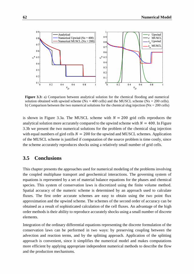
62 Numerical Model

is shown in Figure 3.3a. The MUSCL scheme with 𝑁 = 200 grid cells reproduces the

analytical solution more accurately compared to the upwind scheme with 𝑁 = 400. In Figure

3.3b we present the two numerical solutions for the problem of the chemical slug injection

with equal numbers of gird cells 𝑁 = 200 for the upwind and MUSCL schemes. Application

of the MUSCL scheme is justified if computation of the source problem is time costly, since

the scheme accurately reproduces shocks using a relatively small number of grid cells.

3.5 Conclusions

This chapter presents the approaches used for numerical modeling of the problems involving

the coupled multiphase transport and geochemical interactions. The governing system of

equations is represented by a set of material balance equations for the phases and chemical

species. This system of conservation laws is discretized using the finite volume method.

Spatial accuracy of the numeric scheme is determined by an approach used to calculate

fluxes. The first order accurate schemes are easy to obtain using the two point flux

approximation and the upwind scheme. The schemes of the second order of accuracy can be

obtained as a result of sophisticated calculation of the cell fluxes. An advantage of the high

order methods is their ability to reproduce accurately shocks using a small number of discrete

elements.

Integration of the ordinary differential equations representing the discrete formulation of the

conservation laws can be performed in two ways: by preserving coupling between the

advection and reaction terms, and by the splitting approach. Application of the splitting

approach is convenient, since it simplifies the numerical model and makes computations

more efficient by applying appropriate independent numerical methods to describe the flow

and the production mechanisms.

Figure 3.3: a) Comparison between analytical solution for the chemical flooding and numerical

solution obtained with upwind scheme (Nx = 400 cells) and the MUSCL scheme (Nx = 200 cells).

b) Comparison between the two numerical solutions for the chemical slug injection (Nx = 200 cells)

4

4 Modeling of Dissolution Effects on

Waterflooding

4.1 Introduction

Analysis of coupling of flow and chemical reactions between fluids and porous medium is

an area of interest for many scientific, industrial and engineering processes. A considerable

research is currently focused around injection of the chemistry optimized water by tuning the

salinity and ionic composition in order to increase the recovery [5, 113, 114]. This process

involves a large number of physicochemical interactions, which were partially covered in

Chapter 2. Among others, dissolution and precipitation are two important processes affecting

brine chemistry as they can significantly modify the physical and chemical properties of

porous media [115-118]. Some of the experimental data [36, 119] support the fact that

mineral dissolution takes place during smart water floods and, therefore, its effect should be

quantified.

Similar studies have previously been carried out under the assumption that the fluid was

incompressible [120]. The compressibility of the crude oil-brine-rock system might,

however, be of importance. Both pressure and brine composition (salinity) affect the brine

density. The compositional compressibility may be larger than pressure compressibility. At

the same time, the dissolution may occur under the condition of volumetric disbalance (the

individual volumes of dissolved species will be different from those in the solid state). Thus,

dissolution of a mineral is accompanied by a volume change and a corresponding pressure

adjustment. These changes are probably small, but they may play some role in a confined

space. To account for this effect an equation of state for brine is required. It can be obtained

from the experimental data on the density of electrolyte solutions, available for the specific

ion content of the brine [121, 122].

In this Chapter, a 1D numerical model for two-phase compressible flows with chemical

reactions is presented. An example of such a process is an injection of a weak acid or

carbonated water in a reservoir. A key feature of the model is its capacity to account for the

strong coupling between the fluid flow and mineral reactions that cannot be analyzed

separately. It has turned out that volumetric non-additivity and considerable mass transfer

between phases represent a problem for numerical simulations. Only a fully implicit scheme

seems to be capable of accounting for this effect in the full scale. Therefore, this study was

64 Modeling of Dissolution Effects on Waterflooding

an important step for us to establish a reliable numeric scheme for further applications in our

research.

The structure of this Chapter is as follows. In the first section, we formulate the modifications

that were introduced to the general model for reactive transport described in Chapter 3 and

present the closed system of governing equations. The second section is devoted to the

numerical model and its implementation. In the third section, we describe the results of

numerical simulations. We analyze the changes in reservoir properties introduced by

dissolution, together with the composition of produced water, pressure distribution, and

saturation profiles.

4.2 Model Description

The approach applied in this work is based on the macroscopic approximation of mechanics

of continuous medium, as described in Chapter 2. We consider porous medium initially

saturated with oil and connate water in thermodynamic equilibrium. The rock may be

composed of a number of minerals, which are sensitive to the injected brine composition.

Injection of brine is performed to displace oil, which disturbs the thermodynamic

equilibrium. Namely, the presence of active components in brine causes dissolution and/or

precipitation of minerals. If these processes are intense, they are expected to influence both

flow and reservoir parameters, such as porosity, absolute permeability, residual oil saturation

and, possibly, relative permeability curves. An important difference from similar approaches

used in other studies (e.g. Aharonov et al. [120]) is that we consider a two-phase flow of

compressible fluids. Below we describe the modifications that were introduced in the general

reactive transport model, based on the system of conservation laws presented in Chapter 3.

4.2.1 Mineral Dissolution and Precipitation Reactions

We study non-equilibrium mineral dissolution and precipitation reactions that take place at

the interface between the water and mineral surface. According to classification introduced

by Rubin [123] these reactions are referred as “insufficiently fast” heterogeneous surface

reactions. The general form of dissolution/precipitation reactions of mineral 𝑚 is represented

by:

1

X X 1,...,aqn mm a a ma

m n (4.1)

Variations of molar amounts of aqueous species are related to the mineral reaction rate ��𝑚

via the matrix of the stoichiometric coefficients 𝜈𝑎𝑚:

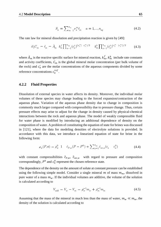
4.2 Model Description 65

1

1,...,mn ma a m aqmS r a n (4.2)

The rate law for mineral dissolution and precipitation reaction is given by [49]:

(| | ( | |)/21

) 21

/ˆ ( ) ( )m m m m

aq aqa a a an nf b

t m m m m a m aa aC r A k c k c (4.3)

where 𝑚 is the reactive specific surface for mineral reaction, 𝑘𝑚𝑓

, 𝑘𝑚𝑏 include rate constants

and activity coefficients, 𝐶𝑚 is the global mineral molar concentration (per bulk volume of

the rock) and 𝑐𝑎′ are the molar concentrations of the aqueous components divided by some

reference concentrations 𝑐𝑎𝑟𝑒𝑓

.

4.2.2 Fluid Properties

Dissolution of external species in water affects its density. Moreover, the individual molar

volumes of these species may change leading to the forced expansion/contraction of the

aqueous phase. Variation of the aqueous phase density due to change in composition is

commonly much larger compared with compressibility due to pressure change. Thus, certain

pressure effects may arise to adjust for the change in density caused by physical-chemical

interactions between the rock and aqueous phase. The model of weakly compressible fluid

for water phase is modified by introducing an additional dependence of density on the

composition of water. A problem of constituting the equation of state for brines was discussed

in [121], where the data for modeling densities of electrolyte solutions is provided. In

accordance with this data, we introduce a linearized equation of state for brine in the

following form:

, 1

0,

0 0ˆ ˆ( )( , ) 1 ( )aqnP w wc aaw w a aP cc P P c cc (4.4)

with constant compressibilities ��𝑃,𝑤, ��𝑤𝑐,𝑎 with regard to pressure and composition

correspondingly, 𝑃0 and 𝑐𝑎0 represent the chosen reference state.

The dependence of the density on the amount of solute at constant pressure can be established

using the following simple model. Consider a single mineral 𝑚 of mass 𝑚𝑚, dissolved in

pure water of a mass 𝑚𝑤. If the individual volumes are additive, the volume of the solution

is calculated according to

1 1add w m w w m mV V V m m (4.5)

Assuming that the mass of the mineral in much less than the mass of water, 𝑚𝑤 ≪ 𝑚𝑤, the

density of the solution is calculated according to

66 Modeling of Dissolution Effects on Waterflooding

00 0

0

1 /1 (1 )

1 ( ) / ( )m w m w w m

add w wadd m ww m m w

m m m m m

V mm m (4.6)

Non-additivity of individual volumes may be accounted via parameter 𝛾 reflecting the change

of the volume of mineral in dissolution: when volume 𝑉𝑚 gets dissolved it becomes 𝑉𝑚(𝑎𝑞) =

(1 + 𝛾)𝑉𝑚. Thus, 𝛾 < 0 corresponds to overall decrease and 𝛾 > 0 to an increase in the

volume of the mixture compared to the sums of initial volumes:

non add add mV V V (4.7)

00 1 (1 (1 ) )m w w m

non add wnon add m w

m m m

V m (4.8)

This simple consideration shows that for small concentrations of solute, compressibility due

to change in composition of the brine can be successfully calculated by the following

dependence

,ˆ 1 (1 ) /wc a m w mc (4.9)

where coefficient 𝛾𝑚 is the relative change in molar volume on the dissolution of mineral 𝑚.

Figure 4.1: Comparison of densities of brine with dissolved CaCO3 (red), MgCO3 (black) and

CaSO4 (blue) calculated from correlations [122], additive mixing and linearized EOS (4.4)

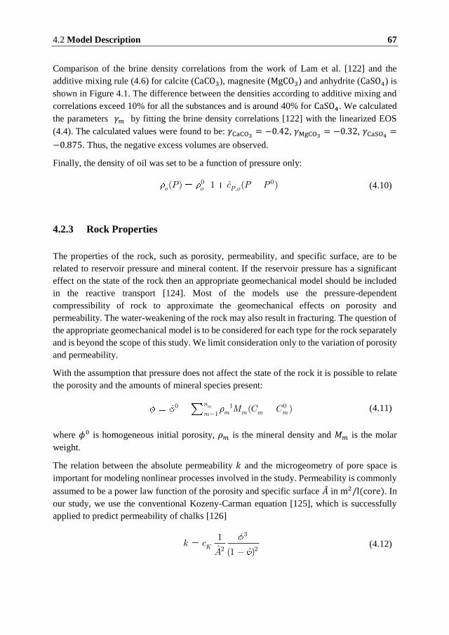
4.2 Model Description 67

Comparison of the brine density correlations from the work of Lam et al. [122] and the

additive mixing rule (4.6) for calcite (CaCO3), magnesite (MgCO3) and anhydrite (CaSO4) is

shown in Figure 4.1. The difference between the densities according to additive mixing and

correlations exceed 10% for all the substances and is around 40% for CaSO4. We calculated

the parameters 𝛾𝑚 by fitting the brine density correlations [122] with the linearized EOS

(4.4). The calculated values were found to be: 𝛾CaCO3 = −0.42, 𝛾MgCO3 = −0.32, 𝛾CaSO =

−0.875. Thus, the negative excess volumes are observed.

Finally, the density of oil was set to be a function of pressure only:

0 0,ˆ( ) 1 ( )Po o o P PcP (4.10)

4.2.3 Rock Properties

The properties of the rock, such as porosity, permeability, and specific surface, are to be

related to reservoir pressure and mineral content. If the reservoir pressure has a significant

effect on the state of the rock then an appropriate geomechanical model should be included

in the reactive transport [124]. Most of the models use the pressure-dependent

compressibility of rock to approximate the geomechanical effects on porosity and

permeability. The water-weakening of the rock may also result in fracturing. The question of

the appropriate geomechanical model is to be considered for each type for the rock separately

and is beyond the scope of this study. We limit consideration only to the variation of porosity

and permeability.

With the assumption that pressure does not affect the state of the rock it is possible to relate

the porosity and the amounts of mineral species present:

0 1 01

( )mnm m m mmM C C (4.11)

where 𝜙0 is homogeneous initial porosity, 𝜌𝑚 is the mineral density and 𝑀𝑚 is the molar

weight.

The relation between the absolute permeability 𝑘 and the microgeometry of pore space is

important for modeling nonlinear processes involved in the study. Permeability is commonly

assumed to be a power law function of the porosity and specific surface in m2/l(core). In

our study, we use the conventional Kozeny-Carman equation [125], which is successfully

applied to predict permeability of chalks [126]

3

2 2

1ˆ (1 )

Kk cA

(4.12)

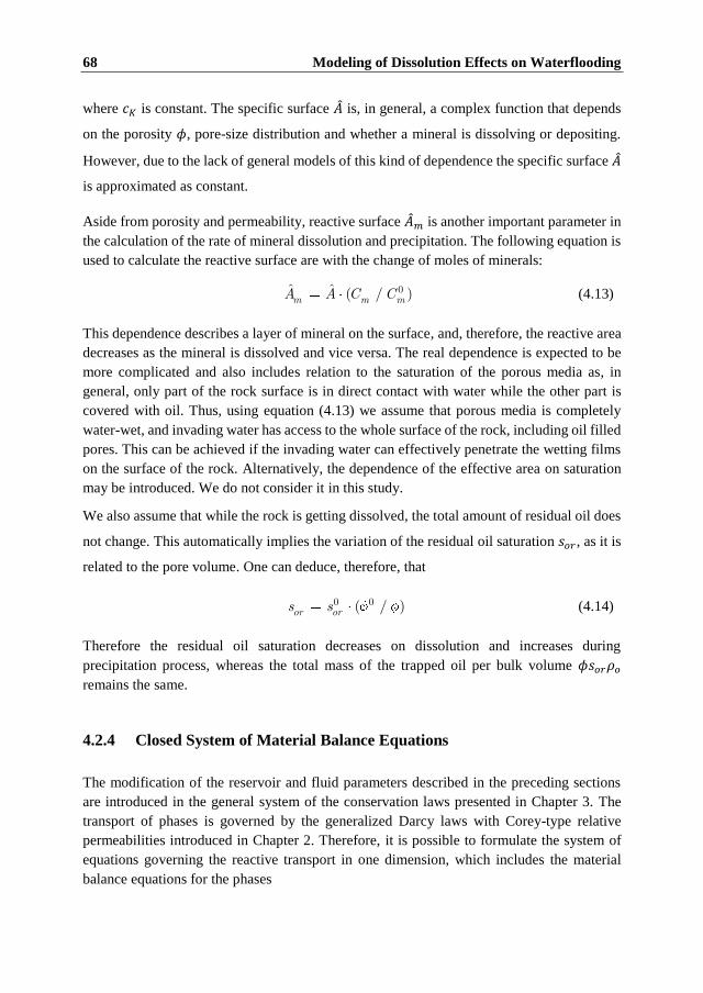
68 Modeling of Dissolution Effects on Waterflooding

where 𝑐𝐾 is constant. The specific surface is, in general, a complex function that depends

on the porosity 𝜙, pore-size distribution and whether a mineral is dissolving or depositing.

However, due to the lack of general models of this kind of dependence the specific surface

is approximated as constant.

Aside from porosity and permeability, reactive surface 𝑚 is another important parameter in

the calculation of the rate of mineral dissolution and precipitation. The following equation is

used to calculate the reactive surface are with the change of moles of minerals:

0ˆ ˆ ( / )m m mA A C C (4.13)

This dependence describes a layer of mineral on the surface, and, therefore, the reactive area

decreases as the mineral is dissolved and vice versa. The real dependence is expected to be

more complicated and also includes relation to the saturation of the porous media as, in

general, only part of the rock surface is in direct contact with water while the other part is

covered with oil. Thus, using equation (4.13) we assume that porous media is completely

water-wet, and invading water has access to the whole surface of the rock, including oil filled

pores. This can be achieved if the invading water can effectively penetrate the wetting films

on the surface of the rock. Alternatively, the dependence of the effective area on saturation

may be introduced. We do not consider it in this study.

We also assume that while the rock is getting dissolved, the total amount of residual oil does

not change. This automatically implies the variation of the residual oil saturation 𝑠𝑜𝑟 , as it is

related to the pore volume. One can deduce, therefore, that

0 0( / )or ors s (4.14)

Therefore the residual oil saturation decreases on dissolution and increases during

precipitation process, whereas the total mass of the trapped oil per bulk volume 𝜙𝑠𝑜𝑟𝜌𝑜

remains the same.

4.2.4 Closed System of Material Balance Equations

The modification of the reservoir and fluid parameters described in the preceding sections

are introduced in the general system of the conservation laws presented in Chapter 3. The

transport of phases is governed by the generalized Darcy laws with Corey-type relative

permeabilities introduced in Chapter 2. Therefore, it is possible to formulate the system of

equations governing the reactive transport in one dimension, which includes the material

balance equations for the phases

4.2 Model Description 69

water: 1

( ( )) aq

t w x wn

w x a aaP M Ss k , (4.15)

oil: ( (1 ) ) ) 0(t o x o o xs k P , (4.16)

rock: 1

((1 ) ) m

t sn

m mmM r , (4.17)

aqueous species:

( ) 1,...) ,( a w x a aqt a x kc P S a nsc , (4.18)

and mineral species:

1,...,t m m mC r m n . (4.19)

where 𝜆𝛼 = 𝑘𝑟𝛼/𝜇𝛼 are the phase mobilities relating the pressure gradient and the linear flow

velocity according to the following equation

( )t w o xu k P (4.20)

Material balance equation for the rock (4.17) may be omitted, due to the fact that porosity is

uniquely related to mineral concentrations via the equation (4.11). Thus, the set of primary

variables includes pressure 𝑃, saturation 𝑠, concentrations of aqueous and mineral species 𝑐𝑎

and 𝐶𝑚 respectively. Equations (4.15)–(4.19) are combined with the closure relations

obtained in preceding sections, namely (4.2) and (4.3) for the mass transfer rates, (4.4) and

(4.10) for densities of the brine and oil, equation (4.11) for porosity and equation (4.12) for

absolute permeability. Finally, the mobilities 𝜆𝛼 are determined through Corey-type relative

permeability functions that account for the change in residual oil saturation according to the

equation (4.14).

The system of material balance equations is to be supplemented with the initial and boundary

conditions. We assume initially homogeneous porous medium saturated with oil at formation

water (FW) at irreducible water saturation, so that initial values of primary variables are:

0( 0, ) , ( 0, )wis t x s P t x P , (4.21)

( 0, ) 1,...,FWa a aqc t x c a n , (4.22)

0( 0, ) 1,...,m m mC t x C m n (4.23)

Our choice of boundary conditions at the inlet corresponds to the injection of brine with fixed

composition at a constant injection rate:

70 Modeling of Dissolution Effects on Waterflooding

0( , 0)t tu t x u , (4.24)

( , 0) 1,...,INJa a aqc t x c a n , (4.25)

while at the outlet it is sufficient to specify pressure

0( , )P t L P (4.26)

4.2.5 Bringing the Equations to a Dimensionless Form

In order to obtain a dimensionless form of the system, we introduce the characteristic length

of between the inlet and outlet 𝐿. The characteristic pressure drop is determined via the

approximate Darcy law:Δ𝑃 = 𝜇𝑤𝑢𝑡0𝐿/𝑘0. The dimensionless variables are defined as

follows:

0

0,D Dx U

x t tL L

(4.27)

0, ,a m

a mrefa m

c CPP c C

P c C (4.28)

0 0 0

( ), , ,

( )ww

kk

k (4.29)

1,...,

ˆm

m mfm

rr m n

Ak (4.30)

The reference values for the molality of aqueous components are usually taken to be 1

mol/kg(H2O) which is approximately the same as refc = 1 mol/l. We use this value for all

the aqueous components. The dimensionless time Dt is measured in multiples of pore

volumes injected, determined with regard to the initial pore volume, as the pore volume will

change with dissolution/precipitation.

The resulting dimensionless system of equations to be solved assumes the form:

1) a( ( ) Dm

DD D

nw x m m mmt w x w P C rs k , (4.31)

4.2 Model Description 71

( (1 ) ) 0) (D D Dt o x o o xs k P , (4.32)

0

1( ) Da( )

D D

m

D

n wa w x mt a x am m mm ref

a m

sc k c P C rc M

, (4.33)

0 0

01,.. ,Da .

D

wmt m mm

m mmC

M CC r m n . (4.34)

where Da𝑚 is the Damköhler number, a dimensionless control parameter for the advection-

reaction problem which we define as

0

0 0Da 1 ..,

ˆ,.m m

m mw

m

t

ALk Mm n

u (4.35)

There are different ways in the literature to define the Damköhler number [120]. However,

the introduced value has a similar physical meaning: it compares the characteristic times of

the convective flow and the chemical equilibration. This ratio is useful to determine whether

the advection rates or reaction rates determine the distribution of aqueous components in the

system. For very small Damköhler numbers (Da ≪ 1), advection occurs much faster than

reaction and thus the distribution of components is very similar with the distribution of inert

tracer in water. At very high Damköhler numbers (Da ≫ 1) the reaction in almost

instantaneous, the equilibrium concentrations are achieved before the flux redistributes the

components. The intermediate values of Damköhler number are of particular interest, as they

represent the behavior of non-idealized systems. It should also be noted that for intermediate

values of Da the reaction terms on the right-hand side of the material balance equation for

water cannot be neglected.

Comparing the Damköhler number for the same reaction taking place during reservoir

flooding and core flood experiments in a similar rock, it can be seen from the equation (4.35)

that the only parameters to change are the length and the linear flow velocity. Applying the

characteristic values we obtain:

,

54

6

0

0,

100 [m] 10 [m/s]10

0.1 [m] 10 [m/s

Da

D ]a

m t labres res

m lab t reslab

uL

L u (4.36)

This simple estimation indicates that at reservoir conditions reactions will exhibit behavior

more similar to equilibrium chemical reactions while under laboratory conditions chemical

kinetics is usually to be taken into account.

72 Modeling of Dissolution Effects on Waterflooding

4.3 Numerical Model

In order to establish a numerical scheme for the presented model, we use the finite volume

formulation as it was described in Chapter 3. The flux between the two neighboring elements

is computed using the two point flux approximation (TPFA). In this case, it is required to

compute geometric parts of the transmissibilities at each time step due to changing absolute

permeability.

4.3.1 Solution Procedure

Initially, our approach was based on the usage of the fully explicit method. Masses of phases

and components were updated at the first step, and the subsequent step was to calculate the

pressure and saturation using the constraint that the sum of all phase volumetric fractions

should be equal to one. However, this approach demanded an extremely small time step, in

order to avoid large changes in pressure. We also tried several other ways of discretization,

making the different variables or their combinations implicit. However, only the fully implicit

scheme seems to really work and produce stable results. This method is computationally

costly per unit step. However, due to better stability it allows for significantly larger time

stepping, making time integration more efficient. We believe that the conventionally used

operator splitting method allowing splitting the integration of the equations into two steps is

not applicable because of the dependence of density on both pressure and composition.

One of the disadvantages of the fully explicit method is the high numerical diffusion. For this

reason, even for fine grids the resulting solution does not reproduce sharp saturation and

concentration fronts. For this study, we considered 300 finite volume cells, which produced

sufficient resolution for comparison between simulations with different parameters.

4.4 Simulation Results

The described model was used to study waterflooding with mineral dissolution. In this

simulation dissolution of a single mineral component and two aqueous components were

considered. The two aqueous components represent the active solute X𝑆 in the water, causing

the dissolution, and a complex X𝐶 which is a combined excess of dissolution reaction so that

stoichiometry of the reaction can be represented by

X X Xm S C (4.37)

The necessary fluid properties are listed in table Table 4.1.

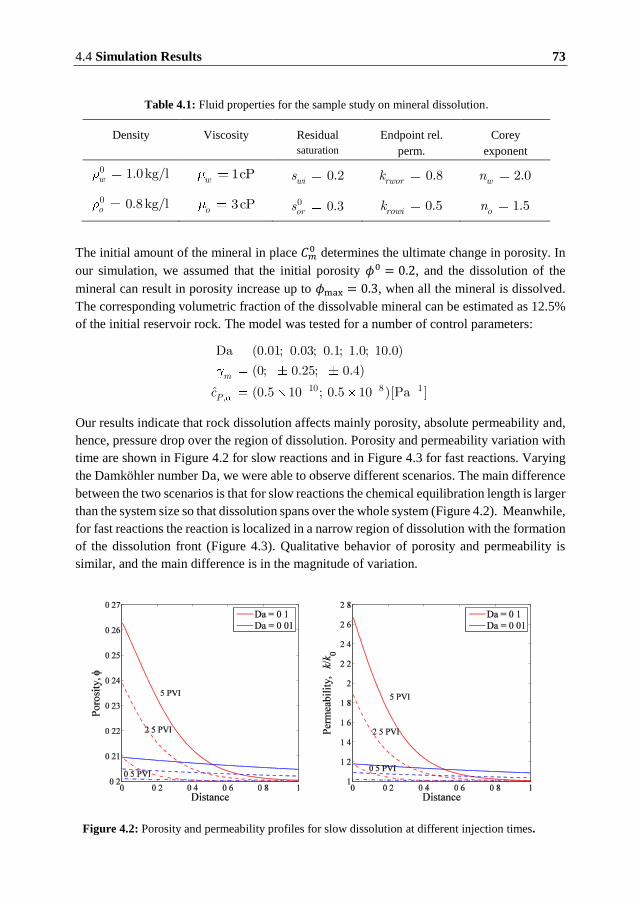
4.4 Simulation Results 73

The initial amount of the mineral in place 𝐶𝑚0 determines the ultimate change in porosity. In

our simulation, we assumed that the initial porosity 𝜙0 = 0.2, and the dissolution of the

mineral can result in porosity increase up to 𝜙max = 0.3, when all the mineral is dissolved.

The corresponding volumetric fraction of the dissolvable mineral can be estimated as 12.5%

of the initial reservoir rock. The model was tested for a number of control parameters:

,10 8 1

0.25;

Da (0.01;

0.4)

ˆ

0.03; 0.1; 1.0; 10.0)

(0;

(0.5 10 ; 0.5 10 )[Pa ]m

Pc

Our results indicate that rock dissolution affects mainly porosity, absolute permeability and,

hence, pressure drop over the region of dissolution. Porosity and permeability variation with

time are shown in Figure 4.2 for slow reactions and in Figure 4.3 for fast reactions. Varying

the Damköhler number Da, we were able to observe different scenarios. The main difference

between the two scenarios is that for slow reactions the chemical equilibration length is larger

than the system size so that dissolution spans over the whole system (Figure 4.2). Meanwhile,

for fast reactions the reaction is localized in a narrow region of dissolution with the formation

of the dissolution front (Figure 4.3). Qualitative behavior of porosity and permeability is

similar, and the main difference is in the magnitude of variation.

Table 4.1: Fluid properties for the sample study on mineral dissolution.

Density Viscosity Residual

saturation

Endpoint rel.

perm.

Corey

exponent

0 1.0kg/lw 1cPw 0.2wis 0.8rwork 2.0wn

0 0.8kg/lo 3cPo 0 0.3ors 0.5rowik 1.5on

Figure 4.2: Porosity and permeability profiles for slow dissolution at different injection times.

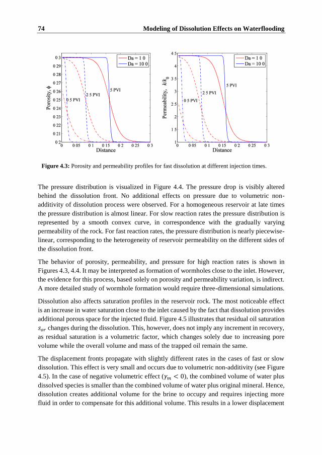
74 Modeling of Dissolution Effects on Waterflooding

The pressure distribution is visualized in Figure 4.4. The pressure drop is visibly altered

behind the dissolution front. No additional effects on pressure due to volumetric non-

additivity of dissolution process were observed. For a homogeneous reservoir at late times

the pressure distribution is almost linear. For slow reaction rates the pressure distribution is

represented by a smooth convex curve, in correspondence with the gradually varying

permeability of the rock. For fast reaction rates, the pressure distribution is nearly piecewise-

linear, corresponding to the heterogeneity of reservoir permeability on the different sides of

the dissolution front.

The behavior of porosity, permeability, and pressure for high reaction rates is shown in

Figures 4.3, 4.4. It may be interpreted as formation of wormholes close to the inlet. However,

the evidence for this process, based solely on porosity and permeability variation, is indirect.

A more detailed study of wormhole formation would require three-dimensional simulations.

Dissolution also affects saturation profiles in the reservoir rock. The most noticeable effect

is an increase in water saturation close to the inlet caused by the fact that dissolution provides

additional porous space for the injected fluid. Figure 4.5 illustrates that residual oil saturation

𝑠𝑜𝑟 changes during the dissolution. This, however, does not imply any increment in recovery,

as residual saturation is a volumetric factor, which changes solely due to increasing pore

volume while the overall volume and mass of the trapped oil remain the same.

The displacement fronts propagate with slightly different rates in the cases of fast or slow

dissolution. This effect is very small and occurs due to volumetric non-additivity (see Figure

4.5). In the case of negative volumetric effect (𝛾𝑚 < 0), the combined volume of water plus

dissolved species is smaller than the combined volume of water plus original mineral. Hence,

dissolution creates additional volume for the brine to occupy and requires injecting more

fluid in order to compensate for this additional volume. This results in a lower displacement

Figure 4.3: Porosity and permeability profiles for fast dissolution at different injection times.

4.4 Simulation Results 75

front velocity. In the opposite case (𝛾𝑚 > 0) velocity of the displacement front slightly

increases.

Propagation of concentration fronts of aqueous components is shown in Figures 4.6, 4.7. The

solute is gradually consumed as it propagates through the porous medium. Depending on the

rates of this consumption, determined by the Damköhler number, the effluent concentration

at the component breakthrough (the time when the components in the injected water will

reach the effluent) will vary as illustrated in Figure 4.8. For higher reaction rates, the solute

will be retarded at the effluent and produced only after many pore volumes of injection

(Figure 4.6c, d). It will not be able to penetrate far from the inlet until complete dissolution

of the mineral. Thus, almost all the injected solute is consumed during the dissolution.

Figure 4.4: Pressure profiles in case of fast and slow dissolution reactions at different injection

times.

Figure 4.5: Saturation profiles in case of fast dissolution with positive and negative volumetric

effects at different injection times.

76 Modeling of Dissolution Effects on Waterflooding

Figure 4.7 illustrates how the complex is produced and washed away by the injected water.

Similarly to the solute, the concentration of complex at the effluent will be determined by the

value of the Damköhler number. Due to the absence of diffusion and other possible

interactions, the sum of the two concentrations is equal to 1. At large Da we can also observe

that the entire available mineral was dissolved in a region close to the inlet after 5 PVI of

injection. The effluent concentrations of the solute for low Da are illustrated in Figure 4.8.

For larger Da, the effluent concentration will be identical, showing itself in a rapid increase

from 0 to 1 at the component breakthrough.

4.5 Conclusions

We developed a 1D numerical model for two-phase multicomponent flow in porous media

accounting for non-equilibrium dissolution and pressure-compositional compressibility of

Figure 4.6: Active solute concentration profiles for different Damköhler numbers.

Figure 4.7: Complex concentration profiles for different Damköhler numbers.

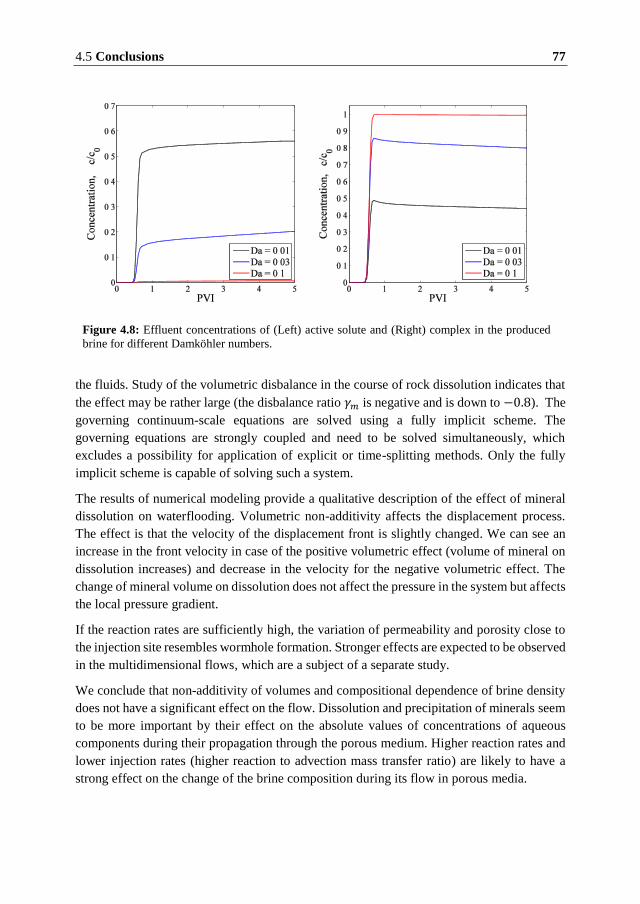
4.5 Conclusions 77

the fluids. Study of the volumetric disbalance in the course of rock dissolution indicates that

the effect may be rather large (the disbalance ratio 𝛾𝑚 is negative and is down to −0.8). The

governing continuum-scale equations are solved using a fully implicit scheme. The

governing equations are strongly coupled and need to be solved simultaneously, which

excludes a possibility for application of explicit or time-splitting methods. Only the fully

implicit scheme is capable of solving such a system.

The results of numerical modeling provide a qualitative description of the effect of mineral

dissolution on waterflooding. Volumetric non-additivity affects the displacement process.

The effect is that the velocity of the displacement front is slightly changed. We can see an

increase in the front velocity in case of the positive volumetric effect (volume of mineral on

dissolution increases) and decrease in the velocity for the negative volumetric effect. The

change of mineral volume on dissolution does not affect the pressure in the system but affects

the local pressure gradient.

If the reaction rates are sufficiently high, the variation of permeability and porosity close to

the injection site resembles wormhole formation. Stronger effects are expected to be observed

in the multidimensional flows, which are a subject of a separate study.

We conclude that non-additivity of volumes and compositional dependence of brine density

does not have a significant effect on the flow. Dissolution and precipitation of minerals seem

to be more important by their effect on the absolute values of concentrations of aqueous

components during their propagation through the porous medium. Higher reaction rates and

lower injection rates (higher reaction to advection mass transfer ratio) are likely to have a

strong effect on the change of the brine composition during its flow in porous media.

Figure 4.8: Effluent concentrations of (Left) active solute and (Right) complex in the produced

brine for different Damköhler numbers.

78 Modeling of Dissolution Effects on Waterflooding

5

5 Micromodel for Two-Phase Flow in

Porous Media

5.1 Introduction

In this Chapter, we address the micromodel for simultaneous flow of water and oil on the

pore scale. The pore space of the rock is characterized by a complex geometry. In order to

take into account its effect on the flow of fluids in porous media, pore-network models may

be used [127]. According to this approach, the porous medium can be effectively represented

as a disordered 3D network constructed of pore bodies.

Pore-network models may be considered as a bridge between the flow at the microscale and

macroscopic displacement. These models take into account the geometry of the pore space

and flow patterns obtained for separate pore bodies depending on the different fluid

configurations [128, 129]. Based on this data pore-network models allow predicting the

transport properties of the rocks and retaining relative permeability curves [130]. The

obtained relative permeability curves can then be applied to describe two-phase flow on the

macroscale. This scheme is, of course, idealized. However, we think that establishing

relations between micro- and macroscale phenomena is important to improve our

understanding of flow in porous media.

In this study, we consider two-phase flow in angular capillaries. This choice of the shape

allows both fluids to be present simultaneously in a capillary [131]. Therefore, it is expected

that the fluids will mutually influence each other during the flow. We consider several

governing parameters to see its effect on the flow; among them are the ratio of fluid

viscosities, boundary conditions at the interphase boundary, and different pressure gradients

in the fluids driving the flow. Of particular interest is the possibility for the flow of one fluid

to induce the flow of another due to action of viscous forces at the interface between the

phases. For a strongly water-wet system, it is also possible that a water film is formed on the

surface of the pore body, and its effect on the flow should also be estimated.

The structure of this Chapter is as follows. In the next section, we present the general

description of triangular capillary and possible fluid configurations. In Section 5.3 we present

the equations governing the two-phase flow in the capillary. Section 5.4 describes the

solution for a single phase problem. In Section 5.5 we consider different possible

configurations of the two-phase flow obtained by different choice of boundary conditions

80 Micromodel for Two-Phase Flow in Porous Media

and different pressure gradients in the fluids. The effect of appearance of the wetting films is

also considered. We present the results by establishing correlation between the flow

velocities of the fluids and wetting fluid saturation. Conclusions and key findings of the study

are presented in Section 0.

5.2 Two-Phase Configurations in Triangular Pores

We consider a two-phase flow in a single triangular capillary. If the non-wetting fluid is

introduced in such a capillary, filaments of the wetting phase (corner films) are formed along

its corners. These filaments are separated from the non-wetting fluid by the arc-menisci

[131]. In this study we assume that the rock is water wet; therefore, oil (non-wetting phase)

occupies the center of the angular capillary, while water resides in the corners. It is also

possible that oil is completely detached from the surface of the rock due to formation of the

water films spreading over entire pore surface.

5.2.1 Characteristics of a Capillary

The geometry of an angular capillary is determined by its length 𝑙, two corner half-angles 𝛽1,

𝛽2, and the hydraulic radius 𝑟ℎ defined as ratio between the capillary cross section area

and its perimeter Π:

hr (5.1)

For a triangular capillary, the hydraulic radius is equal to the half of the radius of inscribed

circle 𝑟0. A schematic representation of a triangular pore cross-section is shown in Figure

5.1. For a pore of a more complex shape, defining the corner half-angles may be problematic,

and its shape is generally characterized in terms of the dimensionless shape factor 𝐺 [132]:

2 20

2 4hr r

G (5.2)

For a triangular pore shape factor may be related to its actual shape according to

13

1

1cot

4 iiG (5.3)

The typical values of the shape factor are the following. The shape factor for a circle 𝐺𝑐𝑖𝑟𝑐 =

1/4𝜋 ≈ 0.079, for a square 𝐺 𝑞 = 0.0625, while for triangles it can take values between

𝐺𝑚𝑎𝑥 = √3/36 ≈ 0.048 for equilateral triangles and 𝐺𝑚𝑖𝑛 = 0 for a slit-like pores.

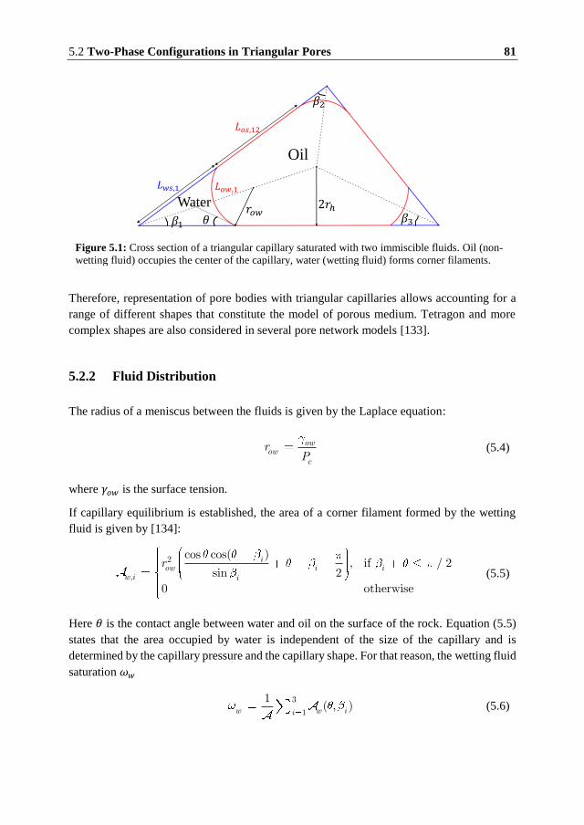
5.2 Two-Phase Configurations in Triangular Pores 81

Therefore, representation of pore bodies with triangular capillaries allows accounting for a

range of different shapes that constitute the model of porous medium. Tetragon and more

complex shapes are also considered in several pore network models [133].

5.2.2 Fluid Distribution

The radius of a meniscus between the fluids is given by the Laplace equation:

owow

c

rP

(5.4)

where 𝛾𝑜𝑤 is the surface tension.

If capillary equilibrium is established, the area of a corner filament formed by the wetting

fluid is given by [134]:

2

,

cos cos( ), if / 2

sin 20 otherwise

iow i i

w i i

r (5.5)

Here 𝜃 is the contact angle between water and oil on the surface of the rock. Equation (5.5)

states that the area occupied by water is independent of the size of the capillary and is

determined by the capillary pressure and the capillary shape. For that reason, the wetting fluid

saturation 𝜔𝑤

3

1

1( , )w w ii

(5.6)

Figure 5.1: Cross section of a triangular capillary saturated with two immiscible fluids. Oil (non-

wetting fluid) occupies the center of the capillary, water (wetting fluid) forms corner filaments.

𝛽1

𝛽2

𝛽3𝜃

2𝑟ℎ𝑟𝑜𝑤

Oil

Water

𝐿𝑤 ,1

𝐿𝑜 ,12

𝐿𝑜𝑤,1

82 Micromodel for Two-Phase Flow in Porous Media

is lower for large pores as it is inversely proportional to the full cross-section area . The

total area of the interface between phases (water-oil, water-solid, oil-solid) is proportional to

the length of the interphase boundary in the cross section and capillary length 𝑙. The lengths

of the interphase boundaries are determined from elementary geometry [134]:

3 3

,1 12

2ow ow i ow ii iL L r (5.7)

3 3,1 1

cos( )2 2

sini

ws ws i owi ii

L L r (5.8)

2h

os ws

rL L

G (5.9)

Equations (5.5), (5.7), and (5.8) are combined to relate the area occupied by water and the

length of the oil-water interface:

2, 2

, , 1

cos cos( )1 ( , )

( ) sin ( 2( ))ow i i

w i ow i ii i

LL S (5.10)

The function 𝑆1(𝜃, 𝛽) increases monotonically with increasing 𝜃. Thus, equation (5.10) states

that the area of the interface between oil and water is higher for low values of the contact

angle.

Equations (5.4) to (5.6) indicate that saturation of water in the capillary is dependent on the

capillary pressure. This saturation is very small at the initial stage of injection, where the

capillary pressure is large. Further, when the capillary pressure decreases, the filaments swell.

At some threshold capillary pressure, the configuration inside the capillary becomes unstable,

resulting in the displacement of oil from the center of the capillary. It is possible, however,

that water already invaded all the surrounding pores, which prevents penetration of oil into

them. If the contact angle changes due to change of wettability towards increased water-

wetness, a thin water film is formed over the entire surface of the capillary, disjoining oil

from the rock surface (Figure 5.2b). Then the oil drops, surrounded by continuous water,

acquire a possibility to move together with the water flow.

5.3 Flow Equations in a Capillary

The flow of the two liquids in a capillary is described as creeping isothermal flow of

incompressible Newtonian fluids with constant viscosities. The flow equations to determine

the velocity field in the cross section of a capillary are the continuity and the Stokes

equations:

5.3 Flow Equations in a Capillary 83

, in , ,v P w o (5.11)

where 𝜇𝛼 is viscosity, 𝑣𝛼 is the fluid velocity, ∇𝑃 is the pressure gradient. We assume that a

constant pressure gradient exists within the fluids ∇𝑃𝛼 = −Δ𝑃𝛼/𝑙 with 𝑧 axis directed along

the length of capillary. Δ𝑣 = 𝜕𝑥2𝑣 + 𝜕𝑦

2𝑣; 𝑥 and 𝑦 represent coordinates in the cross-section

of the capillary. The domain occupied by the phase 𝛼 is denoted with Ω𝛼 , as shown in Figure

5.2.

The no-slip boundary conditions are imposed along the walls of the capillary:

BC0: 0, on , ,sv w o (5.12)

We shall consider two different boundary conditions along the water-oil interface Γ𝑜𝑤. The

first boundary condition requires infinite surface shear viscosity and corresponds to the case

of immobile non-wetting phase:

BC1: 0, on owv (5.13)

The second boundary condition describes the simultaneous flow of two immiscible liquids

separated by an interface, with no momentum transfer across it, as expressed by continuity

in velocity and shear stress:

BC2: , on w w o

owo o

w o

w v n

v v

v n (5.14)

where �� 𝛼 is the unit outward normal vector along Γ𝑜𝑤.

Figure 5.2: Cross section of a triangular capillary saturated with two immiscible fluids. a) Water-

wet with no wetting film present b) Completely water-wet with thin wetting film.

H

O

Γ𝑤

Γ𝑜𝑤Γ 𝑦𝑚,2

Ω𝑤

Ω𝑜

O

Γ𝑤 Γ𝑜

Γ𝑜𝑤

Γ 𝑦𝑚,2

Ω𝑜

Ω𝑤

a) b)

84 Micromodel for Two-Phase Flow in Porous Media

Solving the flow equations (5.11), together with the formulated boundary conditions makes

it possible to calculate average fluid velocities:

1,v v d w o (5.15)

Hydraulic conductances 𝑔𝛼𝛽 are introduced as the proportionality coefficients between the

volumetric flow rate 𝑞𝛼 of the phase and the pressure gradient zP , according to

,

, ,w o

q v d g ov w (5.16)

The form of (5.16) implies that the cross terms are also taken into account for the transport

within the capillary [135, 136].

We consider a dimensionless form of the problem by scaling the spatial coordinates:

20 0 0

, , w

w

vx yx y v

r r r (5.17)

Substitution into (5.11) results in the following system of equations:

0, ,v w o (5.18)

1, , 1,o

w ow

ow o

w

(5.19)

The solution of this dimensionless problem depends only on viscosity ratio ��𝑜, the ratio of

the pressure gradients o , the geometry of the water menisci determined by 𝜃 and 𝑃𝑐, and

the choice of the boundary conditions (BC0 and BC1, or BC0 and BC2). Using the

dimensionless variables, it possible to rewrite equation (5.16) in the form:

4 40 0

,

, ,4 4 w ow

w

w

w v wr r

q gG

oG

(5.20)

where vq is the dimensionless volumetric flux.

As mentioned above, the solution of the flow equations depends on the shape of the capillary.

We limit our study to capillaries which cross-sections are equilateral triangles. Symmetry of

an equilateral triangle allows narrowing the domain by imposing boundary conditions across

the lines of symmetry (Figure 5.2):

5.4 Single-Phase Flow 85

BCs: ,1 ,20, on ,sym symv n (5.21)

The driving force (pressure gradient) of the flow can differ for the two phases. If the oil is

connected to the oil phase at the capillary faces, then we assume that the pressure drops are

equal in the phases. In this case oil in the pore body is a part of an oil cluster and we refer to

it as “active oil”. Another possibility is that oil is disconnected from the oil cluster if

neighboring pores do not contain oil. For such a system oil is present in the pore bodies in a

form of disjoint drops, which we will refer to as “oil ganglia”. The action of capillary forces

at the ends of the capillary can compensate the pressure drop in the oil drop, making ganglia

immobile. However, in the case of a strongly wet surface, formation of wetting films on the

surface of the pore may result in mobilization of oil the drops, so that their flow is driven by

the viscous forces on the oil-water interface.

In order to calculate hydraulic conductances according to equation (5.20), we implemented a

numerical code for the flows in an equilateral triangle into the FlexPDE software [137]. Only

strongly water-wet conditions were investigated (𝜃 < 60∘). According to equation (5.5),

water is always present in the corner filaments. We study several important cases, as

described below.

5.4 Single-Phase Flow

For the single-phase problem, the domain Ω𝑤 fills up the whole capillary. This case is

described by a single equation (5.18) for water with the no-slip boundary condition BC0

(5.12) (We do not mention the symmetry boundary conditions (5.21) hereinafter in the text

as they are just a useful tool to simplify the solution procedure):

0 n

,

o

1

,w

w ws

v

v (5.22)

The resulting average dimensionless velocity is

03

20wv v (5.23)

The volumetric flux calculated according to equation (5.20) is given by

2

5

3w

w

w

qG

(5.24)

Equation (5.23) is generalized for the flow of a fluid with arbitrary viscosity as follows:

86 Micromodel for Two-Phase Flow in Porous Media

0vv (5.25)

This result is in agreement with the single-phase conductance calculated by Patzek and Silin

[132]. Their study supports the conclusion that dependence (5.24) provides a good

approximation for the capillary conductance of triangular capillaries with arbitrary shape

factors 𝐺.

5.5 Two Phase Flow

In this Section, we present the results for several flow configurations in pore bodies occupied

by the two phases. Flow equations (5.18) and no-slip boundary condition on the surface of

the rock BC0 (5.12) are valid for each configuration. The cases differ from each other by the

choice of boundary condition at the oil-water interface: either BC1 (5.13) or BC2 (5.14); and

by the different pressure gradient across the oil phase: either Ξ𝑜 = 0 or Ξ𝑜 = 1. This results

in four different problems. We do not consider a combination of BC1 and Ξ𝑜 = 1 since this

implies that both phases are mobile and can flow, while the boundary between them remain

immobile, which is an obvious contradiction. The rest three cases are discussed below. As

above, we will refer to an oil phase as “active oil” in the cases where the pressure drops in

both fluids are equal, and as “ganglia”, in the cases where the pressure drop in oil is zero.

5.5.1 Flow in the Corner Filaments. Immobile Ganglia

Consider the case of immobile oil phase with the corner flow of the wetting fluid (Figure

5.2a), this may occur due to action of the capillary forces acting at the inlet and outlet of the

capillary. No flow occurs in Ω𝑜 and ��𝑜 = 0. Thus, properties of the oil do not have any

influence on the flow in the corner filaments, and the average water velocity ⟨��𝑤⟩ may only

depend on 𝜃 and 𝑃𝑐. The formulated problem is described by the following system of

equations:

1,

0 on ,

in

,w

w

w

ws ow

v

v (5.26)

Varying the contact angle 𝜃 in the range between 0° and 60°, and 𝜔𝑤 from 0.05 to 𝜔𝑤max

(determined by the highest radius of interface when water menisci do not intersect), we obtain

a correlation for average dimensionless velocity for the flow in corner filaments, shown in

Figure 5.3. The maxiumum wetting fluid saturation 𝜔𝑤max depends on the contact angle 𝜃 and

may be understood by the following consideration. If we fix the endpoints of the meniscus

5.5 Two Phase Flow 87

in the corner and start increasing contact angle 𝜃 the area occupied by the water w will also

increase. The limiting position of menisci, where they meet, is the middle point of the side

of the triangle, the same for all contact angles 𝜃. Hence, the capillary saturation 𝜔𝑤max(𝜃) is

higher for larger values of the contact angle.

It can be seen from Figure 5.3 that a linear dependence can be established between the

average flow velocity ⟨��𝑤⟩ and wetting fluid saturation 𝜔𝑤 for each given value of the contact

angle 𝜃:

1( )w wv C (5.27)

The average flow velocity is slightly lower if the system is more water-wet. This is explained

by a larger length of the oil-water interface according to equation (5.10). A larger immobile

boundary results in enlarged flow resistance, as illustrated in Figure 5.4.

We apply the average value of 𝐶1 to relate the flow velocity to the water saturation, which

does not introduce a significant error:

1w wv C (5.28)

Figure 5.3: Average flow velocity of water in the corner in the case of no-slip boundary condition

at the interface between two fluids for different values of contact angle 𝜃.

Table 5.1: Proportionality coefficients for an average velocity of wetting films and ganglia for the

case of mobile ganglia

𝜃 0° 10° 20° 30° 40° 50° 59° average

𝐶1(𝜃) 0.039 0.040 0.042 0.044 0.046 0.048 0.050 0.046

88 Micromodel for Two-Phase Flow in Porous Media

The average value 𝐶1 = 0.046 was calculated based on all the simulation data presented in

Figure 5.3. The error introduced by averaging in equation (5.28) is admissible, for the three

main reasons:

1. We consider only one possible shape of the triangle.

2. The triangular shape is only an approximation to the real pore shapes.

3. Surface roughness is expected to have an effect on the shape of the corner

filaments.

Similar considerations apply to the rest of the presented results.

5.5.2 Flow of Water and Active Oil

The following calculation represents the case when both water and oil can flow subjected to

equal pressure gradients. The flow of water in the corner filaments is expected to have an

influence on the flow of oil and vice versa. For very viscous oil ��𝑜 ≫ 1, the result should be

similar to the calculated corner flow of water in contact with immobile oil. The governing

system of equations is given by:

0, on ,

, on

1, in ,

1, in ,

, on

,

w

s

w

o o

w o

o

w w o o o

ow

o w

v

v

v v

v

v n v n

(5.29)

Figure 5.4: Dimensionless velocity profiles for corner flow in contact with immobile oil phase for

contact angle of (A) 0° and (B) 50°. Saturation of the wetting phase is equal to 0.35 in both cases.

5.5 Two Phase Flow 89

The contact angle in the computations varied between 0° and 60°. Figure 5.5 shows the

average velocities of fluids; different markers are used for the different contact angles. It can

be seen that variation of the contact angle has stronger effect on the velocity of oil in the case

of high viscosity ratios (Figure 5.5B).

The velocity of the oil phase increases faster with saturation at low values of contact angle.

This is again an effect of the length of the oil-water interface area, which is higher for low

contact angles. As saturation increases, oil is substituted by water in the corners, which can

flow much easier due to lower viscosity. The flow of water facilitates the flow of oil by

increasing the flow velocity at the oil-water interface.

Data shown in Figure 5.5 can be approximated with polynomials:

0

( , ) ( )n

kn o w k o w

k

v P a (5.30)

The second-order polynomial approximation provides a sufficient accuracy:

2

1 2

0 21 2

w ww w w

o oo w w

o

v a a

vv a a

(5.31)

The second equation in (5.31) accounts for the fact that in the case of fully oil saturated pore

the flow velocity is determined by the solution for the single phase problem (5.25).

Correlations (5.31) are plotted in Figure 5.5. The polynomial coefficients based on the

Figure 5.5: Average flow velocity of (A) water and (B) active oil for different viscosity ratios. Solid

lines represent proposed approximations, markers represent simulation data: (plus) 𝜃 = 0∘, (star)

𝜃 = 10∘, (circle) 𝜃 = 20∘, (cross) 𝜃 = 30∘, (square) 𝜃 = 40∘, (diamond) 𝜃 = 50∘, (triangle) 𝜃 =59∘.

90 Micromodel for Two-Phase Flow in Porous Media

simulation data for four different viscosity ratios ��𝑜 = 1, 2, 4, 8 are given in Table 5.2. It can

be seen from the table that deviation from linear behavior for the velocity of water is

relatively low (𝑎2𝑤 ≪ 𝑎1

𝑤) and is observed only at high saturations. The dependence of the oil

flow velocity is more complicated. For the considered viscosity ratios ��𝑜 = 2, 4, 8 , the

effects of increasing wetting fluid saturation are similar (as 𝑎2𝑜 has similar values) and comes

mostly from the second term in the approximation (5.31).

The dependences of the polynomial coefficients 𝑎𝑘𝛼 on the viscosity ratio were established by

applying approximation based on rational functions:

0

0

n kk ok

m kk ok

Qa

R (5.32)

The results of this fitting are presented in Table 5.3. They allow calculating the polynomial

coefficients for the phase flow velocity in the range of viscosity ratios from 1 to 8.

The average velocity of the oil phase may exceed its average velocity in the single-phase

case. The reason is that the corner water occupies the regions where velocity is low due to

proximity to the surface of the capillary. Thus, calculation of the average velocity of oil

includes integration over smaller domains with higher velocities resulting in increased

average velocity.

Table 5.2: Coefficients ka for the polynomial approximation of the average velocity of the corner

flow of water and active oil

��𝑜 = 1 ��𝑜 = 2 ��𝑜 = 4 ��𝑜 = 8

𝑎1𝑤 0.193 0.152 0.107 0.084

𝑎2𝑤 -0.060 -0.026 0.0084 0.0125

𝑎1𝑜 0.138 0.077 0.038 0.017

𝑎2𝑜 0.0032 0.136 0.163 0.134

Table 5.3: Coefficients for the rational function approximation of ka as function of viscosity

𝑄0 𝑄1 𝑄2 𝑄3 𝑅0 𝑅1 𝑅2 𝑅3

𝑎1𝑤 0.312 0.041 - - 1.0 0.835 - -

𝑎2𝑤 -0.086 0.026 - - 1.0 - - 0.0175

𝑎1𝑜 0.557 -0.019 - - 1.0 2.89 - -

𝑎2𝑜 - - - 0.0016 1.0 0.811 0.179 -

5.5 Two Phase Flow 91

To illustrate the effect of the wetting films on the flow of oil we present the calculated

dimensionless flux of oil. Figure 5.6 illustrates the effect. It can be seen that the volumetric

flux of oil decreases only at low viscosity ratios. At high viscosity ratios, it remains the same

or can even increase, as explained above. In Figure 5.7 this effect is illustrated by the plot of

the velocity field in the capillary cross-section.

Figure 5.6: Change of dimensionless volumetric flux of active oil with varying wetting fluid

saturation for different viscosity ratios.

Figure 5.7: Flow velocity profile for water and active oil with increasing water saturation. Oil is

accelerated by the moving oil-water interface (black arc). Contact angle 𝜃 = 50∘, viscosity ratio

𝜇𝑜 = 4.

92 Micromodel for Two-Phase Flow in Porous Media

5.5.3 Flow of Water and Mobile Oil Ganglia

The following calculation represents the case of an oil ganglion, with no pressure drop across

the oil phase. The ganglion may flow carried by the flow of water in the corner filaments due

to continuity of velocity and shear stress at the oil-water interface. The formulated problem

is described by the following system of equations:

0, on ,

1, in ,

0, in ,

,

, o

on

n

,

,

w

s

w o ow

o

w

o o o

w w o o ow

v

v n v n

v

v

v v

(5.33)

As discussed above, the flow may occur when the system is strongly water wet and there are

water films, which cover the whole surface of the pore body as illustrated in Figure 5.2b.

Therefore, we consider a single contact angle 𝜃 = 0∘ and infinitesimally thin wetting film on

the rock surface. The computed average velocities of phases are shown in Figure 5.8.

For this case we make use of the following approximations, which are also illustrated in

Figure 5.8:

1

22

ww w

oo w

v c

v c (5.34)

Figure 5.8: Average flow velocity of (A) water and (B) mobile ganglia oil for 𝜃 = 0∘ and different

viscosity ratios. Markers represent simulation data, solid lines represent proposed approximations

5.5 Two Phase Flow 93

The values of the coefficients 𝑐𝑘𝛼 for different viscosity ratios, and approximation of these

coefficients by rational functions (5.32) as functions of viscosity are given in Tables 5.4, 5.5

respectively. As the viscosity ratio ��𝑜 tends to infinity, 𝑐2𝑤 approaches 𝐶1(0), calculated for

immobile ganglia and 𝑐2𝑜 tends to zero, which is in accordance with the physical nature of

the system.

According to equation (5.34), it is possible to establish a relation between the dimensionless

volumetric flux of oil and water according to

2

21

1( / )(1 )o wo w w

ww w

q c c

q

q

c (5.35)

An important result is that the flux of oil is proportional to the volumetric flux of water and

the area of capillary occupied with oil.

5.5.3.1 Effect of the wetting films on the flow of mobile oil ganglia

We further study the effect of the presence of the wetting films on the surface of the rock, as

illustrated in Figure 5.2b. The thickness of the wetting films in our simulations varied in the

range ℎ = 0 to 0.2 (a fraction of the radius of the inscribed circle 𝑟0). It should be pointed

out that presence of a wetting film does not allow the saturation to fall below a certain limit

that can be calculated according to:

min 21 (1 )w h (5.36)

Table 5.4: Coefficients 𝑐𝑘𝛼 for the polynomial approximation of the average velocity of the corner

flow of water and mobile oil ganglia for 𝜃 = 0∘.

��𝑜 = 1 ��𝑜 = 2 ��𝑜 = 4 ��𝑜 = 8

𝑐1𝑤 0.071 0.064 0.058 0.052

𝑐2𝑜 0.133 0.111 0.086 0.062

Table 5.5: Coefficients for the rational function approximation (𝑄0 +𝑄1𝜇𝑜)/(𝑅0 + 𝑅1𝜇𝑜) of the

coefficients 𝑐𝑘𝛼 as functions of viscosity.

𝑄0 𝑄1 𝑅0 𝑅1

𝑐1𝑤 0.082 0.016 1.0 0.390

𝑐2𝑜 0.157 - 1.0 0.198

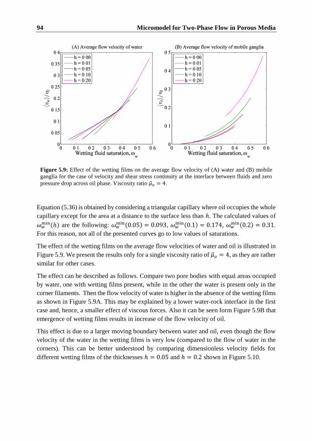
94 Micromodel for Two-Phase Flow in Porous Media

Equation (5.36) is obtained by considering a triangular capillary where oil occupies the whole

capillary except for the area at a distance to the surface less than ℎ. The calculated values of

𝜔𝑤min(ℎ) are the following: 𝜔𝑤

min(0.05) = 0.093, 𝜔𝑤min(0.1) = 0.174, 𝜔𝑤

min(0.2) = 0.31.

For this reason, not all of the presented curves go to low values of saturations.

The effect of the wetting films on the average flow velocities of water and oil is illustrated in

Figure 5.9. We present the results only for a single viscosity ratio of ��𝑜 = 4, as they are rather

similar for other cases.

The effect can be described as follows. Compare two pore bodies with equal areas occupied

by water, one with wetting films present, while in the other the water is present only in the

corner filaments. Then the flow velocity of water is higher in the absence of the wetting films

as shown in Figure 5.9A. This may be explained by a lower water-rock interface in the first

case and, hence, a smaller effect of viscous forces. Also it can be seen form Figure 5.9B that

emergence of wetting films results in increase of the flow velocity of oil.

This effect is due to a larger moving boundary between water and oil, even though the flow

velocity of the water in the wetting films is very low (compared to the flow of water in the

corners). This can be better understood by comparing dimensionless velocity fields for

different wetting films of the thicknesses ℎ = 0.05 and ℎ = 0.2 shown in Figure 5.10.

Figure 5.9: Effect of the wetting films on the average flow velocity of (A) water and (B) mobile

ganglia for the case of velocity and shear stress continuity at the interface between fluids and zero

pressure drop across oil phase. Viscosity ratio 𝜇𝑜 = 4.

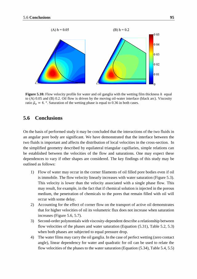
5.6 Conclusions 95

5.6 Conclusions

On the basis of performed study it may be concluded that the interactions of the two fluids in

an angular pore body are significant. We have demonstrated that the interface between the

two fluids is important and affects the distribution of local velocities in the cross-section. In

the simplified geometry described by equilateral triangular capillaries, simple relations can

be established between the velocities of the flow and saturations. One may expect these

dependences to vary if other shapes are considered. The key findings of this study may be

outlined as follows:

1) Flow of water may occur in the corner filaments of oil filled pore bodies even if oil

is immobile. The flow velocity linearly increases with water saturation (Figure 5.3).

This velocity is lower than the velocity associated with a single phase flow. This

may result, for example, in the fact that if chemical solution is injected in the porous

medium, the penetration of chemicals to the pores that remain filled with oil will

occur with some delay.

2) Accounting for the effect of corner flow on the transport of active oil demonstrates

that for higher velocities of oil its volumetric flux does not increase when saturation

increases (Figure 5.6, 5.7).

3) Second-order polynomials with viscosity-dependent describe a relationship between

flow velocities of the phases and water saturation (Equation (5.31), Table 5.2, 5.3)

when both phases are subjected to equal pressure drop.

4) The water films may carry the oil ganglia. In the case of perfect wetting (zero contact

angle), linear dependency for water and quadratic for oil can be used to relate the

flow velocities of the phases to the water saturation (Equation (5.34), Table 5.4, 5.5)

Figure 5.10: Flow velocity profile for water and oil ganglia with the wetting film thickness ℎ equal

to (A) 0.05 and (B) 0.2. Oil flow is driven by the moving oil-water interface (black arc). Viscosity

ratio 𝜇𝑜 = 4. °. Saturation of the wetting phase is equal to 0.36 in both cases.

96 Micromodel for Two-Phase Flow in Porous Media

5) Formation of the wetting films on the surface of the pore bodies results in an

increased flow velocity of oil. The velocity increases more for a larger thickness of

the wetting film. (Figure 5.9B, Figure 5.10)

6) The volumetric flux of mobile oil ganglia is proportional to the volumetric flux of

water in the corner filaments and oil ganglia saturation (Equation (5.35)).

6

6 Tertiary Recovery Model with

Mobilization of Oil Ganglia

6.1 Introduction

Injection of water to displace oil from porous media always results in trapping considerable

amounts of oil in the swept zones. Oil may flow when it forms a continuous phase connected

to the production side (“outlet”). When the oil saturation decreases, more oil drops separate

from the continuous oil cluster. The oil drops (ganglia) are trapped inside the swept zone,

and it is usually assumed that they cannot flow.

In this study, we consider oil displacement by a fluid that contains an agent changing the

wettability, referred to as the active species. Changing of the wettability of the rock results

in mobilization of a part of the residual oil, which is included in the flow. Mobilization may

occur due to the different mechanisms depending on an injected fluid and a type of the rock.

We do not specify or study any specific mechanism. The common idea is that mobilized oil

simply joins the continuous oil phase [92]. One of the core ideas of this chapter is that we

assume a separate transport mechanism for the flow of the mobilized oil in a form of

disconnected oil ganglia. This is a new point of the present work: while the macroscopic

description of flow of the two continuous phases is well established, there is a lack of a model

to describe the flow of a discontinuous phase within porous media [138, 139]. Meanwhile,

as follows from the results of the previous Chapter, such a flow may occur on micro-level.

We develop a mathematical model to describe macroscopic two-phase flow in porous media

accounting for mobile oil ganglia. The system of the flow equations is formulated and solved

numerically. It involves the flows of continuous (“active”) water and oil phases, as well as

of the water films and oil ganglia. The constituting relations for the model (relative

permeabilities and saturations of the different phases) are evaluated by analysis of the flows

in a single capillary and in a capillary network consisting of equal capillaries. This

representation of the porous medium is probably oversimplified, but it gives qualitatively

correct and relatively simple analytical dependencies for the functions required in the model.

The model incorporates analysis of the possible patterns of microscopic two-phase flow in a

separate capillary, presented in Chapter 5, with successive upscaling to obtain macroscopic

flow parameters.

98 Tertiary Recovery Model with Mobilization of Oil Ganglia

The structure of this Chapter is as follows. In the next Section we discuss the mechanisms

that may improve the recovery due to modification of the chemistry of the injected water and,

in particular, explain the mechanism of ganglia mobilization that will be studied in this work.

Section 6.4 contains a formulation of the macroscopic flow model and discussion of its

limitations. In Section 6.5 we describe the way to obtain macroscopic model parameters

based on the pore-scale investigation performed in Chapter 5. We verify the model

predictions by numerical simulation of a tertiary recovery process in Section 6.6.

6.2 Trapping of Oil

Modification of the injected water for enhanced oil recovery may affect the oil production in

two ways. During the secondary water injection starting from low water saturation, an active

substance added to water may affect trapping of the oil ganglia and formation of the

discontinuous oil phase separated from the production site. Since such a discontinuous phase

is difficult to mobilize and produce, the goal at this stage is to decrease the amount of trapped

oil.

Laboratory studies performed on the rock samples after waterflooding experiments support

the fact that prevailing amount of trapped oil is present in a form of oil drops with typical

sizes from one to several pore diameters [68]. Different factors, such as pore geometry,

wettability and injection rate, determine the magnitude of the residual oil and its microscopic

distribution within porous media [140]. Reduction of the residual oil saturation is one of the

most important tasks in the petroleum industry. Different enhanced oil recovery (EOR)

techniques are designed in order to achieve this goal. Among them, the chemical methods

mostly include surfactant-polymer-micellar flooding [140]. Recent studies also address

microbial injection [141, 142] and the smart water flooding [15, 27, 143], which was

discussed in details in Chapter 1.

Numerous experimental and theoretical studies addressed the mechanism controlling

trapping in porous media [68, 144-146]. The instability of two-phase configurations in a thin

throat connecting two oil-filled pores results in a collapse of water films, so that the throat

becomes filled with water. This process is usually referred to as snap-off [67]. As a result,

the connectivity in the oil phase decreases and if snap-off occurs in all the throats surrounding

the oil-filled pore it is completely detached from the oil cluster.

A significant progress in this area of research has been achieved by means of pore-network

simulations. These studies demonstrate that snap-off is a very frequent event among other

possible displacement processes [130] and is strongly dependent on the pore to throat size

ratio and rock wettability. Considering a single pore in a pore-network realization depending

on the externally controlled capillary pressure, it is possible to predict the mechanism by

which this specific pore is filled. This is achieved by means of the method by Mayer, Stowe,

and Princen (MS-P) [147]. Simulated drainage or imbibition processes were used to predict

6.3 Mechanisms of Residual Oil Mobilization 99

quantitatively such important parameters as residual saturations, relative permeabilities, and

phase distribution within the pore-network [128, 148].

The intensity of snap-off is related to the rock wettability. Studies suggest that strongly water-

wet conditions are not favorable for the waterflooding process [149-151]. This is in good

agreement with the findings from the pore-network models [148]. However, the contact angle

measurements on calcite surface demonstrated that for the smart water fluids contact angle

reduces [19, 152]. A possible explanation for this inconsistency in between theoretical

predictions and experiment is that trapping is not affected by the composition of the injected

brine at early stages, since a bank of connate water is formed ahead of the injection brine

[95]. Moreover, if the change of contact angle is not instantaneous and requires a considerable

amount of time, then the effect of wettability alteration will not be seen immediately. Thus,

a transition to a very strong water wet conditions does not result in increased trapping when

performing smart water flooding as a secondary recovery process.

EOR is usually performed not as a secondary, but as a tertiary recovery process. This means

that the residual oil saturation is already formed, and the target for recovery is mostly the

disconnected oil phase. For the tertiary recovery, the mechanism of entrapment of the oil

ganglia is not relevant anymore. The most important problem is what physical mechanisms

may mobilize the discontinuous oil phase and make it moving towards the production site.

6.3 Mechanisms of Residual Oil Mobilization

On the later stage, when the brine saturation is sufficiently large, most of the oil is already in

the form of the oil ganglia. Struggling with trapping cannot produce much at this stage.

Instead, the goal is to mobilize the discontinuous oil phase.

A reason why the discontinuous oil clusters cannot flow is the action of the capillary forces

(the so-called “Jamin effect” [140]. Consider a drop of oil in a capillary surrounded by the

flowing water (Figure 6.1a). A moving force for this drop is the pressure difference in the

water flowing around it. However, instead of being displaced, the oil drop adjusts the

curvatures of menisci in such a way that the difference of capillary pressures compensates

the pressure difference around the drop. The pressure inside the drop remains constant, so

that it does not move. Simple order-of-magnitude estimates show that this capillary effect is

impossible to overcome unless the drop becomes of a macroscopic size or the “global”

pressure difference becomes extremely large.

These considerations are true provided that the drops of oil are attached to the walls of the

capillary. In fact, by analysis of the force balance at the liquid-liquid-solid contact it may be

demonstrated that it is the adhesion forces between liquids and solid (or, the oil-solid and

water-solid surface tensions) that keep the drop attached to the surface.

Consider now the case where water is an absolutely wetting phase, that is, it spreads over the

surface. In such cases, a water film is formed, and it separates the oil from the walls of the

100 Tertiary Recovery Model with Mobilization of Oil Ganglia

pores. If this film flows, the oil drops may slide on its surface (Figure 6.1b). The Jamin effect

does not act anymore.

Assume that during the tertiary recovery stage, an agent changing the reservoir wettability

towards absolutely water wet is injected. Ideally, this may result in formation of moving

water films, disconnection of the oil phase from the surface and additional production of the

discontinuous residual oil. As an example, injection of the brine of a different salinity has

been considered as a possible way to change wettability of the rock [7, 27, 153]. Adsorption

of ions on the calcite or silica surface may also result in changing wettability. Another

possibility is an injection of surfactants [154, 155] or enzymes [156, 157].

An assumption that mobilized oil joins the continuous phase cannot explain multiple

experimental observations, according to which additional oil in e.g. smart flooding

experiments is produced after injection of many porous volumes injected [27, 158-160].

Experimental observations also show that this additional oil may come in the form of

separate drops [161], although this might be explained by the small porous volumes and the

interaction of the oil and the outlet tubing. The velocity of a separate oil drop sliding over the

moving water film will be equal to the surface velocity of this film. Evidently, such velocity

is much lower than the velocities of the continuous oil and water phases. Additionally,

formation of the films may take a while, so that the discontinuous oil flow appears with a

delay. As a result, the additional oil will be produced slowly, after many porous volumes

have been injected.

Absolute wettability is not required for mobilization of, at least, some oil drops. This is only

a condition for rather large pores. For smaller pores, change of wettability may result in a

formation of water films before zero contact angle is achieved. This may explain the relation

between the variation of the contact angle and the expected additional recovery [162].

In this study, we concentrate on the mechanism of the drop mobilization under the tertiary

oil recovery. The model developed below is only applicable to describe this mechanism. For

description of the trapping mechanism additional investigation is required, for example, an

extension of the formalism proposed by P. Bedrikovetsky [139].

Figure 6.1: An oil drop surrounded by water in a capillary. a) Situation of the not completely water

wet rock: origin of the Jamin effect; b) Absolutely water wet rock. Slide of an oil drop over the water

film.

O

Equilibrium menisci

Nonquilibrium menisci

1P 2Pl

OilWater Water

a)

O

1P 2P

OilWater Water

Water film

b)

6.4 Macroscopic Model Formulation 101

6.4 Macroscopic Model Formulation

In order to simulate the effect of presence and mobilization of oil ganglia on waterflooding

of petroleum reservoirs, we apply the traditional approach based on mechanics of continuous

medium. A similar approach was used for the water-alternate-gas injection [163]. Consider a

one-dimensional problem of oil displacement by water containing a chemical. The water

(subscript w) flows as a continuous “active” phase (subscript 𝑎) or as a film (subscript 𝑓).

Oil (subscript o) may also flow as a continuous phase (𝑎) or as ganglia (𝑔). The scheme of

partitioning for the pore space is shown in Figure 6.2. The chemical substance flows with the

injected water and can penetrate the water films in the corners of the oil filled pores and

change the wetting state. When wettability changes significantly, the water films are formed

and the oil ganglia are mobilized. This provides an additional transport mechanism for the

oil phase, contributing to the relative permeability curves.

The mass conservation laws describing the transport of phases that were introduced in

Chapter 2 should be modified in order to account for different transport mechanisms inherent

to each phase:

Water: ( ) 0t x wa wfs u u (6.1)

Oil: ( ) ( ) 0t oa og x oa ogs s u u (6.2)

Species: ( ) ( ) 0t wa wf f x wa fa a w fs c s c u c u c (6.3)

where 𝜙 is porosity, 𝑠 = 𝑠𝑤𝑎 + 𝑠𝑤𝑓 + 𝑠𝑤𝑖 is the overall water saturation, 𝑢 are the velocities

of the different phases (depending on the subscript), 𝑐𝑎 is the molar concentration of the

active species in the water, 𝑐𝑓 is its molar concentration in the water films. The values of 𝑐𝑎

and 𝑐𝑓 may be different. If, for example, the chemical is adsorbed on the surface of the rock,

its concentration close to the surface should be higher than in the bulk. As discussed earlier,

a considerable amount of time may be required for a chemical in order to accumulate in the

water films and to start acting as a wettability modifier; thus, we introduce the kinetic

description of the evolution of 𝑐𝑓:

( ( ) )t f f a fc c c c (6.4)

where 𝜅 is the deposition rate in s-1, and 𝑐��(𝑐𝑎) is the concentration in the water films in

equilibrium with the given bulk concentration 𝑐𝑎, which we will regard as a sorption

isotherm. The velocities are determined via the generalized Darcy laws, for the water phase:

, rwfrwa

wa x w wf x ww w

kkkku P u P , (6.5)

102 Tertiary Recovery Model with Mobilization of Oil Ganglia

( ) rw

w wa wf rwa rwf x w x ww w

kkku u u k k P P , (6.6)

and for the oil phase:

( )roa oa

oa x oo

kk su P , (6.7)

( , )mob

rog ogmobog og wf og x w

w

kk s su u s P (6.8)

rogroao oa og x o x w

o w

kkkku u u P P (6.9)

In these equations, 𝑘 is the absolute rock permeability, 𝜇𝑤 and 𝜇𝑜 are the fluid viscosities,

𝑘𝑟𝛼 are corresponding relative permeabilities, 𝑃𝑤 and 𝑃𝑜 are the pressures in the water and

oil phase respectively. Equation (6.8) assumes that the flow rate of oil ganglia is proportional

to the saturation of mobile oil ganglia 𝑠𝑜𝑔𝑚𝑜𝑏 and the average velocity of water films 𝑢𝑤𝑓

carrying the ganglia, with the proportionality coefficient ( , , )og og o ws that may also

depend on saturation. This coefficient reflects the fact that the average velocity of a film

differs from the velocity of its surface. The corresponding relative permeability is

mobrog og rwf ogk k s . Derivation of equation (6.8) is presented in Section 6.5, based on the

calculation of capillary conductances carried out in Chapter 5. It is important to point out that

Figure 6.2: Structure of the filling of the pore space.

Active oil𝑠𝑜𝑎

Active water𝑠𝑤𝑎

Oil ganglia

𝑠𝑜𝑔Mobile ganglia

𝑠𝑜𝑔𝑚𝑜𝑏

Trapped oil, 𝑠𝑜𝑟

Waterfilms𝑠𝑤𝑓

Oil, 𝑠𝑜Water, 𝑠𝑤𝑠𝑤𝑖

Irreduciblewater

Trapping

6.4 Macroscopic Model Formulation 103

the resulting flow velocity of the oil phase contains a term proportional to the pressure drop

in the water phase, which arises due to the interaction between the two phases.

We neglect the capillary pressure difference, as usual for the Buckley-Leverett scheme [92].

Then the fractional flow function is introduced, determining the amount of water in the flow:

( )( , , )

( ) ( ) ( , )

mob rww oa og

mobwrw ro oa rog og

o

k sf s s s

k s k s k s s

(6.10)

Evolution of oil ganglia saturation is illustrated in Figure 6.3. As the water saturation

gradually increases, starting from 𝑠𝑤𝑖 , the trapping starts. Most of the trapping occurs as

saturation approaches 1 − 𝑠𝑜𝑟0 (where 𝑠𝑜𝑟

0 is the residual oil saturation for “pure”

waterflooding). At the point where water saturation is equal to 1 − 𝑠𝑜𝑟0 , all the oil is in the

form of immobile oil ganglia. Injection of chemical solution will result in the release of part

of the trapped oil and formation of mobile oil ganglia. Further, the flow of mobilized ganglia

will eventually decrease the saturation of trapped oil to 𝑠𝑜𝑟1 . It is also possible that mobile oil

ganglia form an oil bank. As shown in Figure 6.3, the same value of the water saturation may

correspond to the two different oil ganglia saturations, which does not allow to use a closure

relation of the form 𝑠𝑜𝑔 = 𝑠𝑜𝑔(𝑠). This problem will also be discussed in the section devoted

to the limitations of the model.

Equations (6.1) to (6.3), (6.5) to (6.6), (6.10) are combined to obtain

( ) 0t x t ws u f (6.11)

( ( )) ( ) 0rwft wf x t w

rw

ksc s c c c u f

k (6.12)

Figure 6.3: Change of oil ganglia saturation during waterflooding.

𝑠𝑤𝑖 1 − 𝑠𝑜𝑟0

Δ𝑠𝑜𝑟1) Trapping

2) Mobilization

𝑠𝑜𝑔𝑚𝑜𝑏

1 − 𝑠𝑜𝑟1

𝑠𝑤

𝑠𝑜𝑟1

𝑠𝑜𝑟0

𝑠𝑜𝑔

104 Tertiary Recovery Model with Mobilization of Oil Ganglia

where 𝑢𝑡(𝑡) = 𝑢𝑤𝑎 + 𝑢𝑤𝑓 + 𝑢𝑜𝑎 + 𝑢𝑜𝑔 is the overall linear flow velocity determined by the

injection rate. We bring system (6.11), (6.12) to dimensionless form in an ordinary way [92]:

, t

D D

uxx t t

L L (6.13)

/ , /J Ja a f fc c c c c c (6.14)

where 𝑐𝐽 is the molar concentration of chemical in the injected water. Substitution of (6.13)

, (6.14) into (6.4), (6.11) and (6.12) results in

0D Dt x ws f (6.15)

( ( )) ( ) 0

D D

rwft a wf f a x a f a w

rw

ksc s c c c c c f

k (6.16)

1( ) /

D

Jt f f a fc c c c c (6.17)

The initial and boundary conditions assume the form of

0(0, ) 1 , (0, ) 0D or Ds x s c x (6.18)

( ,0) 1, ( ,0) 1w D Df t c t (6.19)

The dimensionless time 𝜏 = 𝜅𝑢𝑡/𝜙𝐿 in Eq. (6.17) is the ratio of the relaxation and

propagation times. As 𝜏 tends to zero (instant relaxation to equilibrium) the species

concentration in the film is determined from the equilibrium relationship

( )f f ac c c (6.20)

The simplest form of dependence (6.20) is the Henry sorption isotherm:

f ac c (6.21)

In the non-equilibrium case, the dimensionless relaxation time 𝜏 is inversely proportional to

the overall length 𝐿. While 𝜏 is finite under laboratory conditions, it becomes very small on

the reservoir scale. Thus, the equilibrium model with the usage of (6.20) instead of (6.17)

should be applied to describe the displacement in the reservoir, while the kinetic model with

(6.17) is to be applied for modeling the laboratory experiments. In Section 6.6 we present

sample calculations for the both cases of sorption and discuss the differences between them.

6.5 Macroscopic Saturations and Permeabilities 105

6.4.1 Features and Limitations of the Model

The most important limitation of the proposed model is that it may only be used for the

description of the tertiary, but not secondary recovery processes. In order for it to be valid, it

is necessary that the oil saturation is close to its residual value. There are the two reasons for

that.

One reason is the assumption of the model that the oil may travel in the form of separate

ganglia. If the oil saturation sufficiently differs from the residual value, such ganglia are

likely to join the continuous oil phase. The percolation theory argues that most of the sites

join the infinite cluster already for the probabilities slightly different from the threshold value

[164]. At a current stage of development, the model cannot include both active oil and mobile

ganglia. This is the main reason to consider tertiary recovery processes in this study.

Another reason for restricted applicability of the model is that it does not account for the

process of trapping/snap off, as discussed above. While the described mechanism requires

that the active substance makes the rock surface more water wet, efficiency of trapping is

related to wettability in a more complex way. A separate model for dynamic trapping is

required.

The proposed model is a two-velocity model for oil movement with the non-instantaneous

release of the second oil “phase”. This release is supposed to be determined by the wettability

conditions; however, this is not important limitation. Any mechanism for non-instantaneous

release of a fraction of the oil phase with a possibility of its slow propagation would result in

a similar model.

A strong limitation of the presented approach is the necessity for additional constituting

dependencies: relative permeabilities 𝑘𝑟𝑤𝑓 , 𝑘𝑟𝑜𝑎 , 𝑘𝑟𝑜𝑔 and fraction 𝑠𝑤𝑓. They should be

expressed in terms of the overall saturation 𝑠, saturation of mobile ganglia 𝑠𝑜𝑔𝑚𝑜𝑏 and

concentrations of the additive on the surface and in the solution. In the next section, we

discuss a relatively simple model making it possible to determine the corresponding

dependencies.

6.5 Macroscopic Saturations and Permeabilities

In this section, we derive the relations for the macroscopic saturation and permeabilities

based on the microscopic consideration of a two-phase flow presented in Chapter 1. The

derived correlations for flow velocities of water and oil (5.31), (5.34) were obtained for a

single capillary and cannot be directly used as the macroscopic permeabilities. An

appropriate upscaling technique is required for that. Generally, this model should be based

on a certain pore-network model, with successive statistical averaging over all the possible

configurations [165]. Here we prefer a simplified treatment, which results in the analytical

formula for relative permeabilities, apparently, without loss of the most important physical

106 Tertiary Recovery Model with Mobilization of Oil Ganglia

effects. In this calculation, we consider porous medium saturated with water and mobile oil

ganglia. The active oil cluster is not present, which corresponds to a large overall water

saturation of porous medium and may be treated as the model for the flow during tertiary

recovery.

A proper upscaling of microscopic conductances should include an ensemble description of

a pore-network. We employ a simplified description, to gain insight into typical relations

between flow parameters and phase distribution within the system. We consider a cross-

section orthogonal to the direction of flow. The average number of capillaries crossing the

unit cross-section area is 𝑛. Its part 𝑦𝑤𝑎 = 𝑛𝑤𝑎/𝑛 is filled with water and belongs to the

infinite water cluster. The rest pores are filled with oil, which is disconnected and forms the

oil ganglia. Their total oil fraction is 𝑦𝑜𝑔 = 𝑛𝑜𝑔/𝑛. The water films are present in the corners

of the oil filled pores; hence, 𝑦𝑤𝑓 = 𝑦𝑜𝑔 = 1 − 𝑦𝑤𝑎. Under the assumption that the system is

translationally invariant, the saturation and the volumetric flow calculated over a given cross-

section will be the same as for the whole system.

The wetting fluid fraction in a capillary is 𝜔𝑤 = 𝜔𝑤(𝜃, 𝑃𝑐). It is assumed that 𝜃 is constant

throughout the system, and that there is a one-to-one correspondence between overall water

saturation 𝑠 and capillary pressure 𝑃𝑐, so that 𝜔𝑤 = 𝜔𝑤(𝑠). The capillary saturation functions

𝜔𝛼, are defined as:

( )

1 )

1

(wf w

o w

a

g

w

s

s

(6.22)

The overall saturations 𝑠𝛼 = 𝜔𝛼𝑦𝛼 for the whole system may then be calculated as follows:

,

(1 ) ,

(1 ) (1 )(1 )

wa wa

wf wf w wa w

og og w wa w

s y

s y s

s y s

(6.23)

The linear velocity 𝑢𝛼 is calculated as the net volumetric flux over the unit cross-section area,

using equation (5.20):

24, ,x

w

Gu n q ny v P wa wf og (6.24)

where 𝑞𝛼 is the volumetric flux of the fluid in a capillary, is the capillary cross-section

area and 𝐺 is the shape factor of the capillary cross-section, ⟨��𝛼⟩ is the dimensionless velocity

in the capillary. The absolute permeability 𝑘 is determined by the volumetric flux calculated

for the single phase problem (5.24):

6.5 Macroscopic Saturations and Permeabilities 107

23

5k nG (6.25)

The relative permeability is calculated as

0

, ,wr

x

u vk y wa wf og

k P v (6.26)

Using the correlations for the phase velocities (5.23) and (5.34) we obtain

rwa wak s (6.27)

1 20 1 ( )w

rwf o wf wk v c y (6.28)

1 20 2( ) (1 )o

rog o og w wk v c y (6.29)

Combining (6.23) together with equations (6.28), (6.29) makes it possible to eliminate 𝜔𝑤,

resulting in

( )rwa wak s s (6.30)

2

1

0

( ) ( )( ) ( ) , ( )

1 ( )

wwf o

rwf rwf o rwf owa

s s ck s C C

s s v (6.31)

2

1

( )( , ) ( ) ( ), ( )

1 ( ) ( )

oog o

rog og rog o rwf rog o wwa o

s ck s s C k s C

s s c (6.32)

where ��𝑜 = 𝜇𝑜/𝜇𝑤 is the viscosity ratio. Equation (6.32) implies that the flow of the oil

ganglia is proportional to the flow of the water films and to the saturation of the oil ganglia,

similarly to (5.35). 𝐶𝑟𝑤𝑓, 𝐶𝑟𝑜𝑔 are constants that depend on viscosity. The values of these

constants may be estimated from equations (5.32), (5.34) with coefficients listed in Tables

5.4, 5.5. The calculated values of these constants for different viscosity ratios are illustrated

in Figure 6.4. Alternatively, 𝐶𝑟𝑤𝑓, 𝐶𝑟𝑜𝑔 may be treated as adjustable parameters.

In order to use the relative permeability function given by equations (6.30) to (6.32), it is

required to specify the water film saturation 𝑠𝑤𝑓(𝑠), active water saturation 𝑠𝑤𝑎(𝑠) and 𝑠𝑜𝑔𝑚𝑜𝑏 .

These dependencies are non-trivial and, as discussed earlier, in general, 𝑠𝑜𝑔𝑚𝑜𝑏 cannot be

introduced as a function of saturation. However, if the active oil phase is not involved, the

overall oil saturation is equal to a sum of the mobile ganglia and residual oil saturations:

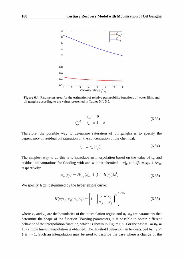
108 Tertiary Recovery Model with Mobilization of Oil Ganglia

0

1oa

mobog or

s

s s s (6.33)

Therefore, the possible way to determine saturation of oil ganglia is to specify the

dependency of residual oil saturation on the concentration of the chemical:

( )or or fs s c (6.34)

The simplest way to do this is to introduce an interpolation based on the value of 𝑐𝑎 and

residual oil saturations for flooding with and without chemical - 𝑠𝑜𝑟1 and 𝑠𝑜𝑟

0 = 𝑠𝑜𝑟1 + Δ𝑠𝑜𝑟

respectively:

0 1( ) ( ) (1 )) (or f f or orfs c H c s H c s (6.35)

We specify 𝐻(x) determined by the hyper ellipse curve:

21

1/

1 2

x x(x;x , x ; , ) 1

x x

nn

LL R

R L

H n n (6.36)

where x𝐿 and x𝑅 are the boundaries of the interpolation region and 𝑛1, 𝑛2 are parameters that

determine the shape of the function. Varying parameters, it is possible to obtain different

behavior of the interpolation function, which is shown in Figure 6.5. For the case 𝑛1 = 𝑛2 =

1, a simple linear interpolation is obtained. The threshold behavior can be described by 𝑛1 ≫

1, 𝑛2 ≈ 1. Such an interpolation may be used to describe the case where a change of the

Figure 6.4: Parameters used for the estimation of relative permeability functions of water films and

oil ganglia according to the values presented in Tables 5.4, 5.5.

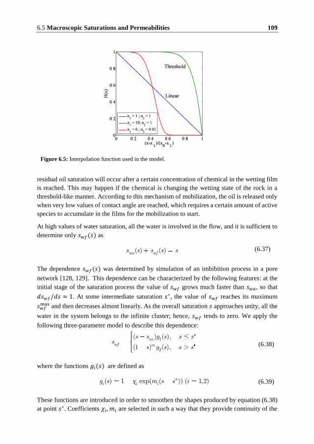
6.5 Macroscopic Saturations and Permeabilities 109

residual oil saturation will occur after a certain concentration of chemical in the wetting film

is reached. This may happen if the chemical is changing the wetting state of the rock in a

threshold-like manner. According to this mechanism of mobilization, the oil is released only

when very low values of contact angle are reached, which requires a certain amount of active

species to accumulate in the films for the mobilization to start.

At high values of water saturation, all the water is involved in the flow, and it is sufficient to

determine only 𝑠𝑤𝑓(𝑠) as

The dependence 𝑠𝑤𝑓(𝑠) was determined by simulation of an imbibition process in a pore

network [128, 129]. This dependence can be characterized by the following features: at the

initial stage of the saturation process the value of 𝑠𝑤𝑓 grows much faster than 𝑠𝑤𝑎, so that

𝑑𝑠𝑤𝑓/𝑑𝑠 ≈ 1. At some intermediate saturation 𝑠∗, the value of 𝑠𝑤𝑓 reaches its maximum

𝑠𝑤𝑓max and then decreases almost linearly. As the overall saturation 𝑠 approaches unity, all the

water in the system belongs to the infinite cluster; hence, 𝑠𝑤𝑓 tends to zero. We apply the

following three-parameter model to describe this dependence:

1

2

( ) ( ),

(1 ) ( ),wi

wf m

s s g s s ss

s g s s s (6.38)

where the functions 𝑔𝑖(𝑠) are defined as

( ) 1 exp( ( )) ( 1,2)i i ig s m s s i (6.39)

These functions are introduced in order to smoothen the shapes produced by equation (6.38)

at point 𝑠∗. Coefficients 𝜒𝑖 , 𝑚𝑖 are selected in such a way that they provide continuity of the

Figure 6.5: Interpolation function used in the model.

( ) ( )wa wfs s s s s (6.37)

110 Tertiary Recovery Model with Mobilization of Oil Ganglia

function and its first derivative. These dependencies contain the three specified parameters:

the pair (𝑠∗; 𝑠𝑤𝑓max) corresponding to the point of the maximum water film saturation, and

parameter 𝑚, which indicates how rapidly saturation of the films decreases after reaching its

maximum value. Comparison between simulated saturations of the wetting films and model

equation (6.38) is presented in Figure 6.6.

Pore network simulations make it possible to establish a relation between the saturation of

oil ganglia and the overall water saturation. Even though it is not used in our model, we

present these results, since they may hopefully be used for future modeling. The behavior of

the oil ganglia saturation function is known from the percolation theory [164, 166]. At low

water saturations, trapping is insignificant. It starts when water saturation reaches some

intermediate value 𝑠∗∗. Further increase in overall saturation results in higher trapping, and

finally, as saturation reaches 1 − 𝑠𝑜𝑟 , all the oil in the system is in the form of ganglia. Further

mobilization of ganglia results in a linear decrease of the saturation of the trapped oil phase.

Simple two-parametric power-law dependence may be used to describe this behavior:

(1 ) , 1( ) 1

1 , 1 ,

l

or orog or

or

s ss s s

s s s ss s s

(6.40)

This equation is valid if no mobile ganglia are present and the local saturation increases with

time: 𝜕𝑡𝑠 > 0. If saturation of water decreases again, this does not necessarily result in

complete mobilization of the previously trapped oil, and equation (6.41) cannot be applied.

The two free parameters in this dependence are 𝑠∗∗, a value of saturation at which trapping

becomes noticeable, and 𝑙 which determines the rate of trapping. The comparison between

simulated saturations of oil ganglia and model equation (6.40) is presented in Figure 6.7.

Figure 6.6: Saturation of water films (A) Pore-network simulation; (B) Model equation (6.38)

6.6 Sample Computations 111

The relative permeability functions of water films and mobile oil ganglia, calculated

according to (6.31), (6.32) are shown in Figure 6.8 with the use of different parameters.

6.6 Sample Computations

The macroscopic displacement problem described by equations (6.15) to (6.19) combined

with relative permeability function given by equations (6.30)-(6.32) and partial saturations

determined according to (6.33), (6.37), (6.38) was solved using the second order accurate

MUSCL-Hancock with 200 finite volume cells.

Figure 6.7: Saturation of oil ganglia (A) Pore-network simulation; (B) Model equation (6.40).

Figure 6.8: Relative permeability functions for (A) water films; (B) mobile oil ganglia.

𝑠𝑤𝑖 = 0.1; 𝑠𝑜𝑟0 = 0.4; Δ𝑠𝑜𝑟 = 0.2; Red: 𝑠∗ = 0.2; 𝑠𝑤𝑓

𝑚𝑎𝑥 = 0.10; Blue: 𝑠∗ = 0.3; 𝑠𝑤𝑓𝑚𝑎𝑥 = 0.15.

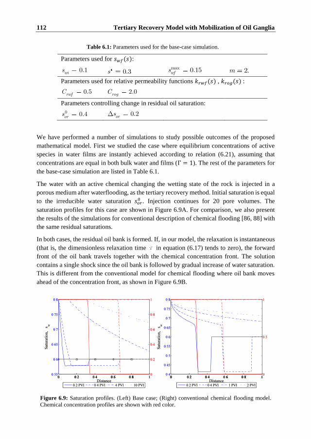
112 Tertiary Recovery Model with Mobilization of Oil Ganglia

We have performed a number of simulations to study possible outcomes of the proposed

mathematical model. First we studied the case where equilibrium concentrations of active

species in water films are instantly achieved according to relation (6.21), assuming that

concentrations are equal in both bulk water and films (Γ = 1). The rest of the parameters for

the base-case simulation are listed in Table 6.1.

The water with an active chemical changing the wetting state of the rock is injected in a

porous medium after waterflooding, as the tertiary recovery method. Initial saturation is equal

to the irreducible water saturation 𝑠𝑜𝑟0 . Injection continues for 20 pore volumes. The

saturation profiles for this case are shown in Figure 6.9A. For comparison, we also present

the results of the simulations for conventional description of chemical flooding [86, 88] with

the same residual saturations.

In both cases, the residual oil bank is formed. If, in our model, the relaxation is instantaneous

(that is, the dimensionless relaxation time in equation (6.17) tends to zero), the forward

front of the oil bank travels together with the chemical concentration front. The solution

contains a single shock since the oil bank is followed by gradual increase of water saturation.

This is different from the conventional model for chemical flooding where oil bank moves

ahead of the concentration front, as shown in Figure 6.9B.

Table 6.1: Parameters used for the base-case simulation.

Parameters used for 𝑠𝑤𝑓(𝑠):

0.1wis 0.3s max 0.15wfs 2.m

Parameters used for relative permeability functions 𝑘𝑟𝑤𝑓(𝑠) , 𝑘𝑟𝑜𝑔(𝑠) :

0.5rwfC 2.0rogC

Parameters controlling change in residual oil saturation:

0 0.4ors 0.2ors

Figure 6.9: Saturation profiles. (Left) Base case; (Right) conventional chemical flooding model.

Chemical concentration profiles are shown with red color.

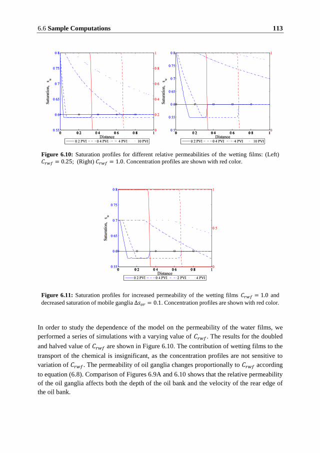
6.6 Sample Computations 113

In order to study the dependence of the model on the permeability of the water films, we

performed a series of simulations with a varying value of 𝐶𝑟𝑤𝑓. The results for the doubled

and halved value of 𝐶𝑟𝑤𝑓 are shown in Figure 6.10. The contribution of wetting films to the

transport of the chemical is insignificant, as the concentration profiles are not sensitive to

variation of 𝐶𝑟𝑤𝑓. The permeability of oil ganglia changes proportionally to 𝐶𝑟𝑤𝑓 according

to equation (6.8). Comparison of Figures 6.9A and 6.10 shows that the relative permeability

of the oil ganglia affects both the depth of the oil bank and the velocity of the rear edge of

the oil bank.

Figure 6.10: Saturation profiles for different relative permeabilities of the wetting films: (Left)

𝐶𝑟𝑤𝑓 = 0.25; (Right) 𝐶𝑟𝑤𝑓 = 1.0. Concentration profiles are shown with red color.

Figure 6.11: Saturation profiles for increased permeability of the wetting films 𝐶𝑟𝑤𝑓 = 1.0 and

decreased saturation of mobile ganglia Δ𝑠𝑜𝑟 = 0.1. Concentration profiles are shown with red color.

114 Tertiary Recovery Model with Mobilization of Oil Ganglia

Variation of the value of Δ𝑠𝑜𝑟 (the maxiumum amount of oil to be mobilized by the chemical)

demonstrated similar results. Increasing permeability of wetting films by increasing 𝐶𝑟𝑤𝑓

twice and reducing Δ𝑠𝑜𝑟 by half almost reproduced the base case curves (Figure 6.11).

The difference may be observed when comparing the incremental recovery curves, shown in

Figure 6.12. It illustrates that increased permeability of wetting films allows achieving final

recovery faster. Meanwhile, decreasing Δ𝑠𝑜𝑟 allows producing all the mobile oil faster at the

same permeability (Figure 6.12B).

Introduction of the non-equilibrium sorption may result in a significant delay of the forward

front of the disconnected oil. There are essentially two parameters, which effects should be

studied. The first parameter is the dimensionless relaxation time 𝜏, which determines the rate

of chemical deposition. The value of 𝜏 equal to one corresponds to the deposition rate of

2500 s−1 at a typical laboratory conditions 𝐿 = 10 cm, 𝑢𝑡 = 10−5 m/s, 𝜙 = 0.25. The

second parameter is the shape of the interpolation function 𝐻, which indirectly determines

the rate of oil mobilization. For a linear interpolation function, the rate of oil mobilization is

determined by the deposition rate of the chemical; for a non-linear interpolation function the

rate of oil mobilization additionally depends on the amount of the active species accumulated

in the film.

First, we studied the effect of the sorption kinetics, using the linear interpolation function for

the residual oil saturation. In this case, the release of oil starts immediately as chemical starts

to accumulate in the water films. The results of simulations with different relaxation times 𝜏

are illustrated by the recovery curves in Figure 6.13A. The non-equilibrium kinetics, in this

case, does not affect the arrival of the oil bank. The non-instantaneous release of oil ganglia

results in a decreased depth of the oil bank as less oil is involved in the flow. This can be

seen by a slower increase in recovery after the arrival of the oil bank.

Figure 6.12: Incremental recovery. (Left) Varying the relative permeability of wetting films; (Right)

Varying the amount of the mobile oil ganglia.

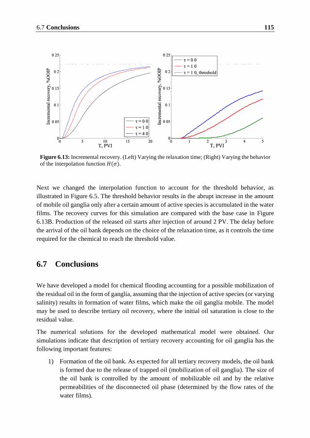
6.7 Conclusions 115

Next we changed the interpolation function to account for the threshold behavior, as

illustrated in Figure 6.5. The threshold behavior results in the abrupt increase in the amount

of mobile oil ganglia only after a certain amount of active species is accumulated in the water

films. The recovery curves for this simulation are compared with the base case in Figure

6.13B. Production of the released oil starts after injection of around 2 PV. The delay before

the arrival of the oil bank depends on the choice of the relaxation time, as it controls the time

required for the chemical to reach the threshold value.

6.7 Conclusions

We have developed a model for chemical flooding accounting for a possible mobilization of

the residual oil in the form of ganglia, assuming that the injection of active species (or varying

salinity) results in formation of water films, which make the oil ganglia mobile. The model

may be used to describe tertiary oil recovery, where the initial oil saturation is close to the

residual value.

The numerical solutions for the developed mathematical model were obtained. Our

simulations indicate that description of tertiary recovery accounting for oil ganglia has the

following important features:

1) Formation of the oil bank. As expected for all tertiary recovery models, the oil bank

is formed due to the release of trapped oil (mobilization of oil ganglia). The size of

the oil bank is controlled by the amount of mobilizable oil and by the relative

permeabilities of the disconnected oil phase (determined by the flow rates of the

water films).

Figure 6.13: Incremental recovery. (Left) Varying the relaxation time; (Right) Varying the behavior

of the interpolation function 𝐻(𝜎).

116 Tertiary Recovery Model with Mobilization of Oil Ganglia

2) The velocity of the forward front of the oil bank is controlled by the concentration

front of active solute. If the chemical equilibrium between the bulk and the water

films is achieved instantaneously, the velocity of the forward front is equal to the

propagation rate of the chemical. This result is different from the conventional

model of chemical flooding, where the concentration front controls the rear front of

the oil bank.

3) Introduction of the non-equilibrium sorption of the active species in the water films

will result in a slower increase in recovery with no additional delay of the oil bank.

4) Accounting for threshold behavior of ganglia mobilization may result in additional

delay of the arrival of the residual oil bank. The delay may be up to several pore

volumes injected (depending on the equilibration time)

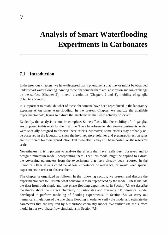
7

7 Analysis of Smart Waterflooding

Experiments in Carbonates

7.1 Introduction

In the previous chapters, we have discussed many phenomena that may or might be observed

under smart water flooding. Among these phenomena there are: adsorption and ion exchange

on the surface (Chapter 2), mineral dissolution (Chapters 2 and 4), mobility of ganglia

(Chapters 5 and 6).

It is important to establish, what of these phenomena have been reproduced in the laboratory

experiments on smart waterflooding. In the present Chapter, we analyze the available

experimental data, trying to extract the mechanisms that were actually observed.

Evidently, this analysis cannot be complete. Some effects, like the mobility of oil ganglia,

are proposed in this work for the first time. There have been no laboratory experiments, which

were specially designed to observe these effects. Moreover, some effects may probably not

be observed in the laboratory, since the involved pore volumes and pressures/injection rates

are insufficient for their reproduction. But these effects may still be important on the reservoir

scale.

Nevertheless, it is important to analyze the effects that have really been observed and to

design a minimum model incorporating them. Then this model might be applied to extract

the governing parameters from the experiments that have already been reported in the

literature. Other effects could be of less importance or relevance, or would need special

experiments in order to observe them.

The chapter is organized as follows. In the following section, we present and discuss the

experimental data to illustrate what behavior is to be reproduced by the model. These include

the data from both single and two-phase flooding experiments. In Section 7.3 we describe

the theory about the surface chemistry of carbonates and present a 1D numerical model

developed to perform modeling of flooding experiments. In Section 7.4 we carry out

numerical simulations of the one phase flooding in order to verify the model and estimate the

parameters that are required by our surface chemistry model. We further use the surface

model in our two-phase flow simulations in Section 7.5.

118 Analysis of Smart Waterflooding Experiments in Carbonates

7.2 Summary of Experimental Data

In order to study the surface chemistry, it is important to have experimental data on the single-

phase and two-phase flows on the same rock, with measurements of the concentrations of the

potential determining ions in the effluent. It is important that fluid injection in the two-phase

experiments is fast so that viscous forces dominate or play an important role. Slow

experiments on spontaneous imbibition may provide additional information. Also, the fast

two-phase experiments should be compared to fast single-phase flow-through experiments

for the same rock, where the concentrations of the ions in the effluent are measured.

The necessity to distinguish between fast and slow flows arises since (as we discuss below)

there may be two mechanisms that are responsible for ion exchange with the surface.

Adsorption of the ions is relatively fast and reversible. Meanwhile, under longer times the

irreversible chemical reactions of dissolution-precipitation of the rock become prevailing.

Comparison of fast and slow flow-through experiments demonstrates qualitatively different

pictures of ion production (see comparison below). That is why fast and slow experiments

should be considered separately.

We have selected the experimental data with the flow rates exceeding 5PV per day, or,

approximately, 0.1 ml/min. The sets of experiments that have been selected for the present

work have been carried out with Stevns Klint rock samples. To the best of our knowledge,

the experiments discussed at the present Chapter are the only sets of such experiments that

have reported all the necessary parameters, at least, in comparison with each other. We

compare single-phase and two-phase such experiments. Separately, we compare fast and

slow flow-through experiments and discuss the qualitative difference between the observed

distributions of the ions in the produced effluent.

7.2.1 Fast Single-Phase Flow Experiments

An extensive study on the on the wetting properties of carbonates was carried out by Austad

and co-workers [5-7, 14, 26, 32, 167]. These experiments were mainly performed with the

Stevns Klint outcrop chalk, which is characterized by relatively low permeability of 2 −

4 mD, porosity 𝜙 of 45 − 50% , and weight surface area 𝑤 of 2 m2/g [168]. The amount

of impurities is usually low. In most experiments, that we will review, an approximate pore

volume of the core plugs was around 40 ml.

A study performed by Strand et al. [32] included spontaneous imbibition tests and

chromatographic analysis of the ions in the effluent. The last analysis is important for

recovering the simulation parameters for our model and, therefore, will be discussed in detail.

The cores were initially 100% saturated with the seawater-like brine containing no sulfate.

The brine injected in the core contained sulfate together with thiocyanate (SCN−) in equal

amounts. It is suggested that thiocyanate does not interact with the surface of carbonate, and,

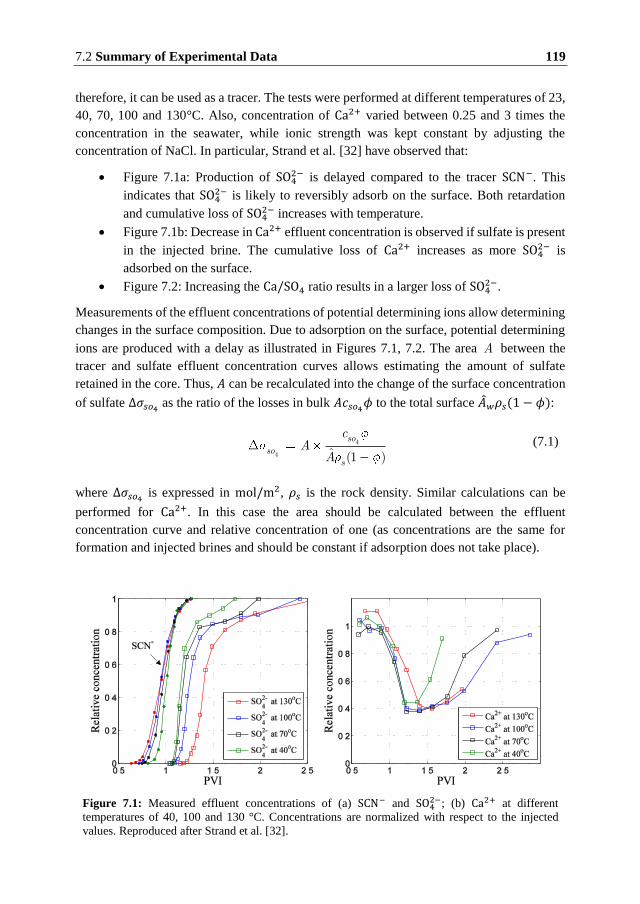
7.2 Summary of Experimental Data 119

therefore, it can be used as a tracer. The tests were performed at different temperatures of 23,

40, 70, 100 and 130°C. Also, concentration of Ca2+ varied between 0.25 and 3 times the

concentration in the seawater, while ionic strength was kept constant by adjusting the

concentration of NaCl. In particular, Strand et al. [32] have observed that:

Figure 7.1a: Production of SO42− is delayed compared to the tracer SCN−. This

indicates that SO42− is likely to reversibly adsorb on the surface. Both retardation

and cumulative loss of SO42− increases with temperature.

Figure 7.1b: Decrease in Ca2+ effluent concentration is observed if sulfate is present

in the injected brine. The cumulative loss of Ca2+ increases as more SO42− is

adsorbed on the surface.

Figure 7.2: Increasing the Ca/SO4 ratio results in a larger loss of SO42−.

Measurements of the effluent concentrations of potential determining ions allow determining

changes in the surface composition. Due to adsorption on the surface, potential determining

ions are produced with a delay as illustrated in Figures 7.1, 7.2. The area A between the

tracer and sulfate effluent concentration curves allows estimating the amount of sulfate

retained in the core. Thus, can be recalculated into the change of the surface concentration

of sulfate Δ𝜎 𝑜 as the ratio of the losses in bulk 𝑐 𝑜 𝜙 to the total surface 𝑤𝜌 (1 − 𝜙):

4

4 (1ˆ )

soso

sA

cA (7.1)

where Δ𝜎 𝑜 is expressed in mol/m2, 𝜌 is the rock density. Similar calculations can be

performed for Ca2+. In this case the area should be calculated between the effluent

concentration curve and relative concentration of one (as concentrations are the same for

formation and injected brines and should be constant if adsorption does not take place).

Figure 7.1: Measured effluent concentrations of (a) SCN− and SO42−; (b) Ca2+ at different

temperatures of 40, 100 and 130 °C. Concentrations are normalized with respect to the injected

values. Reproduced after Strand et al. [32].

120 Analysis of Smart Waterflooding Experiments in Carbonates

In order to understand the interplay between the two cations we consider the studies of Zhang

et al. [5] and Strand et al. [6]. Though different lithology of the rocks may result in different

properties, we believe that it is important that more experimental data is presented for further

discussion. In the first work affinities of Ca2+and Mg2+ towards the surface of the Stevns

Klint chalk were studied at 23°C and 130°C. The core plugs were initially saturated with

0.573M NaCl brine and flooded with the CF-M brine (see Table 7.1) with equal

concentrations of Ca2+and Mg2+, while SO42− was not present.

The study of Zhang et al. [5] on the sorption of cations demonstrates the following:

Figure 7.3a: At 23°C more Ca2+ is adsorbed on the surface.

Figure 7.3b: At 130°C delay in production of both cations is almost equal. Further

increase in Ca2+ concentration indicates that Mg2+can substitute Ca2+ on the

surface.

Figure 7.2: Measured effluent concentrations of SO42− awith varied concentration of Ca2+ in the

brines. (a) 130°C; (b) 70°C. Concentrations are normalized with respect to the injected values.

Reproduced after Strand et al. [32].

Table 7.1: Brine composition for the studies of Strand et al. [32], Zhang et al. [5], Zahid et al. [8]

Ion SW SW-U SW-M SW1/2Ca SW2Ca CF-M ZP SW1S SW0S SW3S

Na+ 0.560 0.510 0.484 0.472 0.435 0.504 0.573 0.368 0.378 0.348

Mg2+ 0.045 0.045 0.045 0.045 0.045 0.013 0.000 0.045 0.045 0.045

Ca2+ 0.013 0.013 0.013 0.006 0.026 0.013 0.000 0.013 0.013 0.013

Cl− 0.525 0.623 0.525 0.524 0.526 0.556 0.573 0.434 0.492 0.317

SO42− 0.024 0.000 0.024 0.024 0.024 0.000 0.000 0.024 0.000 0.072

HCO3− 0.002 0.002 0.002 0.002 0.002 0.002 0.000 0.002 0.002 0.002

SCN− 0.000 0.000 0.024 0.024 0.024 0.013 0.000 - - -

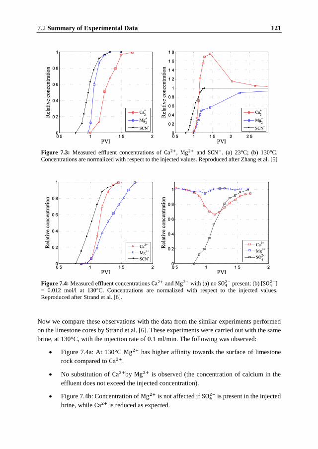
7.2 Summary of Experimental Data 121

Now we compare these observations with the data from the similar experiments performed

on the limestone cores by Strand et al. [6]. These experiments were carried out with the same

brine, at 130°C, with the injection rate of 0.1 ml/min. The following was observed:

Figure 7.4a: At 130°C Mg2+ has higher affinity towards the surface of limestone

rock compared to Ca2+.

No substitution of Ca2+by Mg2+ is observed (the concentration of calcium in the

effluent does not exceed the injected concentration).

Figure 7.4b: Concentration of Mg2+ is not affected if SO42− is present in the injected

brine, while Ca2+ is reduced as expected.

Figure 7.3: Measured effluent concentrations of Ca2+, Mg2+ and SCN−. (a) 23°C; (b) 130°C.

Concentrations are normalized with respect to the injected values. Reproduced after Zhang et al. [5]

Figure 7.4: Measured effluent concentrations Ca2+ and Mg2+ with (a) no SO42− present; (b) [SO4

2−]

= 0.012 mol/l at 130°C. Concentrations are normalized with respect to the injected values.

Reproduced after Strand et al. [6].

122 Analysis of Smart Waterflooding Experiments in Carbonates

We believe that these observations are not fully consistent with each other, at least, if the ion

substitution on the surface is a trusted mechanism. In the absence of sulfate, the magnesium

ions are definitely preferred by the surface (Figure 7.4a). Presence of sulfate would reduce

the positive surface charges and, therefore, increase this preference. Meanwhile, almost no

adsorption of magnesium is observed in the presence of sulfate, while calcium still gets

adsorbed (Figure 7.4b). Further discussion of this effect may be found below.

7.2.2 Comparison of Fast and Slow Flow-Through Experiments

Other studies address primarily slow injection of the modified seawater [57, 169]. During

slow injection, composition of the brine produced in the effluent is much stronger affected

by the mineral dissolution and precipitation reactions, as observed in some of the experiments

[5, 57]. Similar to the results described in Chapter 4, presence of mineral reactions will result

in the steady-state distribution of the concentrations in the brine between the inlet and outlet

[170]. We will list the observations from these studies that are important for further

discussion:

At low injection rates of approximately 0.01 ml/min and high temperatures, increase

in Ca2+ and an almost equal decrease in Mg2+ is observed in the effluent. This may

be an indication of calcite dissolution accompanied by the formation of a

magnesium-bearing mineral [33].

SO42− can be released from the surface if distilled water is injected [169].

As illustrated by the experimental data, Mg2+ can substitute Ca2+ both at low and high

injection rates. In particular, the two different ways for such substitution should be

distinguished. First, the substitution is possible on the sorption sites of the calcite surface due

to higher affinity of this surface to the cations. This substitution is expected to increase

concentration of Ca2+ (at low temperatures) for a short while. However, at high temperatures

in several studies [6, 57, 167] a long-lasting substitution of calcium by magnesium was

observed: during more than 5 pore volumes of injection, experimentally observed effluent

concentrations of both cations were different from their injected values. The changes in cation

concentrations were close by absolute value but opposite. Hiorth et al. [33] suggested that

this substitution is likely to occur through combined dissolution/precipitation mechanism:

dissolution of calcite and subsequent precipitation of magnesium-bearing mineral (e.g.

huntite (Mg3Ca(CO3)4 as suggested by Madland et al. [34]). This process is observed only

at low injection rates and, therefore, should not influence concentrations of Ca2+ and Mg2+

in the experiments performed under high injection rates.

Sorption is considered to be a fast process, and, therefore, governs the fluid-rock interactions

at high injection rates and early stages of flooding. On the contrary, mineral dissolution and

precipitation processes are generally characterized by much lower rates [71, 72]. The

magnitude of the effect of dissolution and precipitation on the concentrations in brine is

determined by the ratios of the reaction rates to the convective flow rates (as expressed by

7.2 Summary of Experimental Data 123

the Damköhler numbers). It depends on the rates of reactions, flow velocity and the distance

between the inlet and outlet. The reaction rates of the brines with the carbonates may vary

several orders of magnitude [76]. Therefore, exact determination of the Damköhler numbers

is impossible. However, the results of the considered experiments look like the slow-rate

experiments are carried out with the Damköhler numbers of the order of unity while the fast

experiments correspond to the numbers much less than one. Forced core flood experiments

are usually performed with high injection rates 𝑞𝑖𝑛𝑗 > 0.1 ml/min on the core plugs with a

typical length of 10 cm. For such experiments it is likely that mineral reactions are slow

compared to convective transport and have only minor effect on ion concentrations. It is

additionally confirmed by the discussed experiments. In all of them concentrations of the

potential determining ions were reaching their injected values after at least 3 pore volumes

of injection (Figures 6.1-6.4), while in cases of irreversible chemical reactions this would

never happen. For that reason, mineral reactions are not considered in our model for fast

experiments.

7.2.3 Two-phase Flow Experiments

We consider now the two-phase flooding experiments performed by Zahid et al. [8]. One of

the reasons for this particular choice is that these experiments were also performed on the

Stevns Klint outcrop chalk. Other studies were performed on the carbonate reservoir and

outcrop cores [21, 30] and demonstrated that potential of the smart water flooding is also

dependent on a rock material.

In the experiments conducted by Zahid et al. [8] the core plugs were completely saturated

with oil and flooded at different temperatures of 40, 90, 110 and 130°C, with the injection

rate of 5 PV/day (approximately 0.1 ml/min). The brines used in these experiments were

similar to the ones used in the chromatographic studies, with a slightly lower ionic strength

(see Table 7.1).

No aging was performed after core saturation and, therefore, the rock could be considered to

be completely water wet, as some amount of water was possibly still present in the rock in a

form of the wetting films. Most tests were performed with the Latin American (LA) oil

(density 0.846 g/cm3, viscosity 13.3 cP, AN = 0.163 mg KOH/g, BN = 0.563 mg KOH/g).

Only four tests were carried out with the North Sea (NS) and the Middle East (ME) oils.

These oils are different mainly by acid and base numbers: for North Sea oil: AN =

0.095 mg KOH/g, BN = 2. 442 mg KOH/g; for Middle East oil: AN = 0.093 mg KOH/g,

BN = 0.644 mg KOH/g. Table 7.2 summarizes the data on the oil recovery for these

experiments. Some of the recovery curves are also presented in Figure 7.5.

We will briefly summarize the observations for the experiments involving the Latin

American and the Middle East oils:

124 Analysis of Smart Waterflooding Experiments in Carbonates

Final recovery achieved by seawater without sulfate (SW0S) remains similar at all

the temperatures. Perhaps, a small increase is observed at higher temperatures.

Injection of seawater (SW1S) and seawater reach in sulfate (SW3S) after SW0S

brine in all cases resulted in additional recovery.

Under equal temperatures, the effect SW3S injection was more pronounced

compared to the injection of SW1S brine.

Recovery for the injection of both SW1S and SW3S brines increased with

temperature.

Additional oil was produced within approximately 1 PV of injection.

An increase of recovery with temperature for the injection of SW0S brine may be partially

explained by a more favorable mobility ratio. Viscosity of oil at low temperatures is relatively

high and is expected to decrease when the temperature is raised.

Secondary flooding experiments demonstrated similar oil recoveries for all types of oil used

in the study. Meanwhile, the increase in recovery with SW3S brine during tertiary flooding

was negligible in Test 10, performed with the North Sea oil. It is not clear what factor caused

the difference. One of the influencing factors is, perhaps, a much higher base number of the

North Sea oil. However, we believe that the number of experiments with the North Sea oil is

not sufficient to make far going conclusions.

Similar increases in recovery were observed in the secondary and the tertiary recovery modes,

which indicates that history of flooding does not influence the final state of the rock surface.

As under secondary flooding, the additional recovery was observed within approximately 1

PV of injection. The oil banks seem to come before or simultaneously with the concentration

fronts. There is no reason to assume the action of the ganglia mechanism that was modeled

in Chapter 6. Therefore, modeling of the available experimental data may be carried out

within the standard models of two-phase flow with the convection-dispersion mechanism of

the propagation of the ions, and accounting for adsorption of these ions on the rock surface.

There is no seeming reason to go for a more complex model, at least, based on the available

experimental data.

7.2.4 Discussion of the Experimental Data

Probably, the most controversial data are presented in Figures 6.3 and 6.4. First of all, the

calculated area 𝑐𝑎 between the tracer and Ca2+ effluent concentration curve (Figure 7.3) is

−0.535. Negative value of 𝑐𝑎 indicates that Ca2+ is not accumulated in the core due to

adsorption; instead, the produced amount of Ca2+ is larger than injected. The formation brine

(ZP) does not contain any Ca2+ and, therefore, there are the two possibilities: 1) a sufficient

amount of Ca2+ was initially adsorbed on the surface, but for some reasons could not desorb

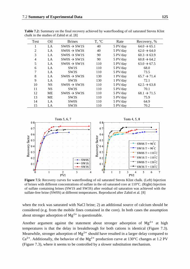
7.2 Summary of Experimental Data 125

when the rock was saturated with NaCl brine; 2) an additional source of calcium should be

considered (e.g. from the mobile fines contained in the core). In both cases the assumption

about stronger adsorption of Mg2+ is questionable.

Another argument against the statement about stronger adsorption of Mg2+ at high

temperatures is that the delay in breakthrough for both cations is identical (Figure 7.3).

Meanwhile, stronger adsorption of Mg2+ should have resulted in a larger delay compared to

Ca2+. Additionally, the behavior of the Mg2+ production curve at 130°C changes at 1.2 PV

(Figure 7.3), where it seems to be controlled by a slower substitution mechanism.

Table 7.2: Summary on the final recovery achieved by waterflooding of oil saturated Stevns Klint

chalk in the studies of Zahid et al. [8]

Test Oil Brines T, °C Rate Recovery, %

1 LA SW0S → SW1S 40 5 PV/day 64.0 → 65.1

2 LA SW0S → SW3S 40 5 PV/day 62.0 → 64.0

3 LA SW0S → SW1S 90 5 PV/day 60.3 → 63.9

4 LA SW0S → SW1S 90 5 PV/day 60.8 → 64.2

5 LA SW0S → SW1S 110 5 PV/day 63.0 → 67.5

6 LA SW1S 110 5 PV/day 68.0

7 LA SW3S 110 5 PV/day 73.5

8 LA SW0S → SW3S 130 1 PV/day 65.7 → 71.4

9 LA SW3S 130 1 PV/day 72.1

10 NS SW0S → SW3S 110 5 PV/day 62.5 → 63.8

11 NS SW3S 110 5 PV/day 70.1

12 ME SW0S → SW3S 110 5 PV/day 68.1 → 71.5

13 ME SW3S 110 5 PV/day 75.9

14 LA SW0S 110 5 PV/day 64.9

15 LA SW3S 110 5 PV/day 70.2

Figure 7.5: Recovery curves for waterflooding of oil saturated Stevns Klint chalk. (Left) Injection

of brines with different concentrations of sulfate in the oil saturated core at 110°C. (Right) Injection

of sulfate containing brines (SW1S and SW3S) after residual oil saturation was achieved with the

sulfate-free brine (SW0S) at different temperatures. Reproduced after Zahid et al. [8]

126 Analysis of Smart Waterflooding Experiments in Carbonates

It is important to mention that substitution of Ca2+ by Mg2+ was not observed in experiments

performed on the limestone cores (Figure 7.4a). Mg2+ was still slightly stronger adsorbed on

the surface in the absence of sulfate. This implies that on the injection of seawater in the core,

the variation of the Mg2+ concentration should be greater than that of Ca2+. The results of

the corresponding experiment, shown in Figure 7.4b, do not confirm the expected behavior:

only substantial decrease of Ca2+ concentration is observed while concertation of Mg2+

remains unchanged.

Finally, there is a question of the repeatability of the experimental data. Most of the presented

experiments were performed once, and the range of variation in the measured effluent

concentration curves is not known.

If we compare observations from the flow-through experiments and two-phase displacement

experiments, there is an indication that increase in recovery corresponds to a change in the

surface composition. The analysis of the experimental data indicates that

Conditions favorable for recovery: increased temperature and larger concentration

of sulfate in the injected brine, correspond to an increased concentration of sulfate

on the surface.

Adsorption of sulfate has an effect on adsorption of calcium and magnesium through

the change of the surface charge.

Hence, a minimum model fitting reasonably reproducible results of the experiments should

include consideration of the surface composition. Adsorption of all of the potential

determining ions should be considered simultaneously and the surface charge should be

introduced as a parameter governing the adsorption process.

7.3 Model Formulation

In this section, we describe the mathematical model to account for the adsorption of potential

determining ions on the surface of the rock and its effects on the flooding efficiency. This is

achieved by combining the surface chemistry model with a 1D Buckley-Leverett model

presented in Chapter 2. The single phase flow is described as a special case with water

saturation equal to unity. For the two-phase flow, the parameters determining the relative

permeability curves are assumed to be dependent on the surface concentrations of adsorbed

ions. This approach is similar to the one used in modeling of the low salinity effects on

waterflooding [171].

7.3.1 Surface Chemistry

A model for description of the surface chemistry should take in account that adsorption of

the different ions takes place on the charged surface of calcite. This charge changes the

7.3 Model Formulation 127

affinity of ions towards the surface. A relevant description is provided by the surface

complexation model of carbonate surface developed in [5, 6, 33, 55, 172]. Analysis of these

studies reveals a certain variation in parameters that are used for modeling of fluid-rock

interactions.

According to the model, adsorption of potential determining ions takes place on two different

surface complexes: > CO3− and > CaOH2

+. Exchange reactions between surface sites and

aqueous species, that were presented in Chapter 2, result in the following possible

configurations of surface complexes (species): > CO3−, > CO3H

0, > CO3Ca+, > CO3Mg

+, >

CaOH0, > CaOH2+, > CaSO4

−, > CaCO3−. Several studies [33, 55] on thermodynamic

equilibria of carbonate surface in contact with seawater-like brines claim that at pH from 7

to 9, and low bicarbonate concentrations the most abundant surface species are: > CO3−, >

CO3Ca+, > CO3Mg

+, > CaOH2+, > CaSO4

−. Therefore, it is sufficient to account only for the

following adsorption reactions:

23 3>CO Mg >CO Mg (7.2)

23 3>CO Ca >CO Ca (7.3)

22 4 4 2>CaOH SO >CaSO H O (7.4)

Presence of charged complexes on the surface results in non-zero surface charge density 𝛿

which is calculated according to:

s s

s

s a aa

z (7.5)

where summation is performed over all charged surface species; 𝜎𝑎𝑠 represents the surface

concentration of the species in [mol/m2]; and ℱ is the Faraday constant, ℱ = 96485 C/mol.

An important parameter that influences the sorption capacity of the surface is the site density

𝑑 , which for carbonate rocks is estimated to be between 2 and 5 sites/nm2 [33, 55] and

equal for both > CO3− and > CaOH2

+. The site density can be recalculated into sorption

capacity: 𝑇 = 𝑑 /𝑁𝐴 = 3.32 to 8.85 μmol/m2. We estimate the number of moles of

aqueous species per unit surface of the rock to be around 1.85 μmol/m2 for 0.01M solution.

A large value of 𝑇 indicates that the surface can accommodate large amounts of adsorbed

species and has strong influence on the brine composition. It is also convenient to describe

composition of the surface in terms of the surface mole fractions:

/s sa a sT (7.6)

Applying eq. (7.6) one can express the surface charge density in terms of surface mole

fractions of the potential determining ions:

128 Analysis of Smart Waterflooding Experiments in Carbonates

4

2 ( )s s ca mg soT (7.7)

The surface charge density determines the surface potential , which affects activities of

ions close to the surface. The surface potential is calculated using the Gouy-Chapman theory

[75, 82]:

3

08 10 sinh2

ss RT I

RT (7.8)

where 휀 is the dielectric constant of water, 휀0 is the permittivity of the free space, 휀0 =

8.854 × 10−12 C2/(m ⋅ J), 𝑅 is the universal gas constant, 𝑇 is the absolute temperature, 𝐼 is

the ionic strength (molal).

The equilibrium conditions for the surface reactions (7.2)-(7.4) are described by the mass

action equations:

3 2

1 23

[>CO Mg ]=

[>CO ][Mg ]K (7.9)

3 2

2 23

[>CO Ca ]=

[>CO ][Ca ]K (7.10)

4 2 2

3 22 4

[>CaSO ][H O]=

[>CaOH ][SO ]K (7.11)

exp /s RT (7.12)

where [X] denotes the activity of a species X; 𝐾1, 𝐾2 and 𝐾3 are equilibrium constants

dependent on temperature. Additional exponential term 𝜒 accounts for the interactions of the

ions with the charged surface. It decreases the activities of ions with the charge of the same

sign as that of the surface, and increases the activities of species with opposite charge.

The activities of the surface species are taken to be equal to their mole fractions 𝛽𝑎𝑠 [72]. The

activities of species in the aqueous solution are related to molar concentrations: 𝑎𝑎 =

𝛾𝑎𝑐𝑎/𝑐𝑎⊖

, where 𝑐𝑎⊖

is the reference concentration. The activity coefficients 𝛾𝑎 can be

calculated with the Davis equation:

210log 0.3

1a a

IAz I

I (7.13)

7.3 Model Formulation 129

where A is the temperature dependent constant and 𝑧𝑎 is the valence of the species. In our

model we account also for complexation between potential determining ions: CaSO4(𝑎𝑞) and

MgSO4(𝑎𝑞). Formation of complexes is more pronounced at high temperatures and can

significantly affect the activity of Mg2+. In order to take this into account we performed the

PHREEQC simulations [173] for the seawater (SW and SW1S in Table 7.1) varying the

concentration of SO42−, and computed the activity coefficients for Ca2+, Mg2+ and SO4

2− as

functions of 𝑐 𝑜 . For a given temperature these dependences were used to calculate the

activity coefficients of the potential determining ions.

The surface mole fractions for complexes > CO3− and > CaOH2

+ are 𝛽𝑋 = 1 − 𝛽𝑐𝑎 − 𝛽𝑚𝑔 and

𝛽𝑌 = 1 − 𝛽 𝑜 respectively. Based on equations (7.9)-(7.11), the equilibrium surface mole

fractions can be expressed in the form:

21

2 21 21

mgmg

mg ca

K a

K a K a (7.14)

22

2 21 21

caca

mg ca

K a

K a K a (7.15)

4

4

4

23

231

soso

so

K a

K a (7.16)

It should be noted that apparent similarity of sorption isotherms (7.14)-(7.16) with Langmuir

sorption isotherms is misleading. The electrostatic exponential term 𝜒 is dependent on ��𝑎𝑠 ,

and therefore the equilibrium surface composition cannot be calculated explicitly.

Dielectric permittivity of water appears in equation (7.8) and is known to vary with

temperature and ionic strength of brine [174, 175]. The variation with temperature is from 80

at 23°C to 50 at 130°C. We applied the correlation for the permittivity suggested in [25].

Ionic strength in the discussed experiments was kept around the same level, hence, we assume

휀 to be constant. However, we believe that effect of ionic strength may be pronounced when

salinity of the brine varies significantly (e.g. low salinity flooding).

The input parameters, that are required by this surface chemistry model are:

Equilibrium constants for adsorption reactions 𝐾1, 𝐾2, 𝐾3.

Site density 𝑑 (we apply 𝑑 = 5 sites/nm2).

Specific surface area of the rock.

130 Analysis of Smart Waterflooding Experiments in Carbonates

7.3.2 The Transport Model

Below we present the 1D transport model for a two-phase flow of water (w) and oil (o). It is

based on the Buckley-Leverett model for incompressible fluids [92]. It was described in

details in Chapter 2; here we will briefly outline the major points. The equations for the

single-phase flow are a special case of the derived system with the water saturation equal to

unity.

The flow of phases is determined according to the generalized Darcy law:

,xu k P w o (7.17)

where 𝑘 is the absolute permeability, 𝜆𝛼 is the phase mobility, 𝑃 is the pressure. Additional

dependence on the molar fractions of adsorbed species is introduced in the phase mobilities

𝜆𝛼. This is done in Section 7.5 by correlating observed experimental oil recovery with the

predicted equilibrium surface composition for different brines and temperatures.

We assume that initially present formation brine is in equilibrium with the surface of the

rock, corresponding to the composition 𝛽𝑎0 of the adsorbed species. As saturation increases,

part of the surface 𝛼𝑟 is put in contact with the injected water, while the rest is in contact with

the formation water. Therefore, adsorption process takes place only on the fraction 𝛼𝑟 of the

surface, and composition 𝛽𝑎0 remains unchanged on the fraction 1 − 𝛼𝑟 of the surface. The

global concentrations of adsorbed species (per unit volume of the porous medium) are given

by:

0ˆ ( (1 ) )a s r a r ac AT (7.18)

where is the specific surface area in m2/l(core). Porosity and absolute permeability are

considered to be constant and fluids are assumed to be incompressible. This results in

constancy of the linear flow velocity 𝑢𝑡:

( )t w o w o xu u u k P (7.19)

Therefore, we can use the fractional flow formulation and disregard pressure from the

computations. The system of material balance equations for the components is obtained in

accordance with the description given in Chapter 3:

0t w t x ws u f (7.20)

0ˆ( ( (1 ) )) ( ) 0t w a s a a t x a ws c AT u c f (7.21)

04

ˆ( ( (1 ) )) Ca,Mg,SOsorbt s r a r a aAT r a (7.22)

7.3 Model Formulation 131

where ��𝑎 𝑜𝑟𝑏 is the sorption rate, which we is defined as follows:

4

ˆ ( / ) Ca,Mg,SOazssorba r

orba aAk I Pr AP IA K a (7.23)

where 𝐼 𝑃+ and 𝐼 𝑃− are the ion activity products for a forward and backward reactions, as

defined in (7.2)-(7.4), and 𝐾𝑎′ includes the electrostatic term 𝜒. For the reaction of

magnesium sorption the rate law (7.23) reads:

21

ˆ ( / ( ))sorbmg mg X m

sorbm gg rAk a Kr (7.24)

Sorption rates for the rest of the reactions (7.3), (7.4) are calculated correspondingly. This

approach allows calculating both equilibrium and non-equilibrium surface reactions by

tuning the reaction rate constants. The limiting case of the infinite rate constants corresponds

to the equilibrium sorption [92].

The fraction of the reactive surface in contact with brine 𝛼𝑟 ∈ [0,1] should be related to

saturation. It increases with saturation between zero, for a fully oil saturated core, and one,

for a fully water saturated core. The simplest model is

r ws (7.25)

The effect of pore-size distribution and presence of wetting films are likely to modify this

dependence. At this stage of the model development, the actual dependence on the saturation

was found not to play an important role and we use equation (7.25) without any

modifications.

7.3.3 Numerical Model

The numerical methods used in our studies were covered in Chapter 3. We used the finite

volume formulation with discretized domain consisting of 80 cells. The ratio of the time step

to the space step was 1/10. With this choice, the numerical diffusion was of the same order

of magnitude as the typical values of the convective diffusion in a porous medium. The match

was assessed by comparison of the tracer effluent concentration curves in experiments and

model calculations since dispersion is the only mechanism affecting the wash-out of the

tracer production curves.

The advection and reaction terms were treated separately. According to this approach, each

time step is split into advection and reaction sub-steps. During the advection sub-step, only

transport terms are considered in equations (7.20), (7.21) and solution for saturation and new

aqueous concentrations is updated using forward Euler method. During the reactions step

only equations containing reaction terms (7.22) are considered. The reaction step was treated

implicitly. The solution of the system of non-linear equations representing (7.22) was

obtained using the solver from the Fortran minpack library [111].

132 Analysis of Smart Waterflooding Experiments in Carbonates

7.4 Numerical Modeling of the Single Phase Experiments

All the simulations presented in this work were performed with the constant sorption rate

constants 𝑘𝑎 𝑜𝑟𝑏. The choice of significantly large rate constants results in contracted

transition zone of species concentrations between injection and formation values compared

to the experimental curves. Usage of significantly small rate constants results in earlier

breakthrough and broad transitions zone with intermediate concentrations. We found that the

choice 𝑘 𝑜𝑟𝑏 = {300,300, 600} mol ∙ s−1/m3(core) resembled the width of the transition

zone observed in the experiments relatively well.

As a first step, we performed modeling of the co-adsorption of Ca2+ and SO42− and compared

it with the experimental data from the study of Strand et al. [32]. As concentration of Mg2+

is not reported in the study, there is an ambiguity in determining the equilibrium constants

𝐾𝑎 and different sets of 𝐾𝑎 can give a reasonable fit. The values used in our simulations were

obtained using a trial and error method. We also compared the equilibrium constants with the

rest of our simulations, requiring that all equilibrium constants 𝐾𝑎 are of the same order of

magnitude as reported in [33, 55]. Table 7.3 summarizes the equilibrium constants used in

our simulations. Simulation results for these experiments are shown in Figures 7.6, 7.7.

At low temperatures of 40°C and 70°C the model captures the qualitative behavior reasonably

well (Figure 7.6). It clearly demonstrates that adsorption of sulfate on the surface will result

in additional adsorption of Ca2+ from the solution, as observed by the decreased effluent

concentration. Same is true for the simulations performed at high temperatures (Figure 7.7).

In this case, the discrepancy with experimental data is more significant for the concentration

of Ca2+, while the effluent concentration of SO42− is reproduced relatively well. The main

inconsistency is that our model does not predict a long-term decrease in calcium

concentration. According to model formulation, adsorption of sulfate results in the co-

adsorption of cations, therefore, variation of concentrations should be observed at the effluent

during a similar time.

Table 7.3: Summary on the equilibrium constants used in simulations

Description T, °C 𝐾1 𝐾2 𝐾3 Figure

ZP → CF-M 23°C 20 50 - 7.10

SW-U → SW-M 23°C 20 50 30 7.6

SW-U → SW-M 40°C 20 70 35 7.6

SW-U → SW-M 70°C 30 80 40 7.8

SW-U → SW-M (xCa) 70°C 15 120 45 7.9

SW-U → SW-M 100°C 60 120 60 7.7

ZP → CF-M 130°C 1000 200 - 7.11, 7.12

SW-U → SW-M 130°C 100 200 110 7.7, 7.8

SW-U → SW-M (xCa) 130°C 55 300 120 7.9

7.4 Numerical Modeling of the Single Phase Experiments 133

Figure 7.6: Modeled and experimentally measured effluent concentrations of Ca2+and SO42− at low

temperatures: (Upper) 23°C (𝐾1 = 20,𝐾2 = 50,𝐾3 = 30); (Lower) 40°C (𝐾1 = 20, 𝐾2 = 70,𝐾3 =35). SW-M brine is injected in the chalk core initially saturated with SW-U brine.

Figure 7.7: Modeled and experimentally measured effluent concentrations of Ca2+and SO42− at high

temperatures: (Upper) 110°C (𝐾1 = 60,𝐾2 = 120,𝐾3 = 60); (Lower) 130°C (𝐾1 = 100,𝐾2 =200,𝐾3 = 110). SW-M brine is injected in the chalk core initially saturated with SW-U brine.

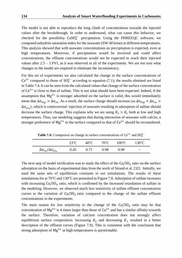
134 Analysis of Smart Waterflooding Experiments in Carbonates

The model is not able to reproduce the long climb of concentrations towards the injected

values after the breakthrough. In order to understand, what can cause this behavior, we

checked for the possibility CaSO42− precipitation. Using the PHREEQC software, we

computed anhydrite saturation index for the seawater (SW-M brine) at different temperatures.

This analysis showed that with seawater concentrations no precipitation is expected, even at

high temperatures. Moreover, if precipitation would be involved and could affect

concentrations, the effluent concentrations would not be expected to reach their injected

values after 2.5 – 3 PVI, as it was observed in all of the experiments. We are not sure what

changes in the model are required to eliminate the inconsistency.

For this set of experiments we also calculated the change in the surface concentrations of

Ca2+ compared to those of SO42− according to equation (7.1); the results obtained are listed

in Table 7.4. It can be seen from the calculated values that change of the surface concentration

of Ca2+ is close to that of sulfate. This is not what should have been expected. Indeed, if the

assumption that Mg2+ is stronger adsorbed on the surface is valid, this would immediately

mean that Δσ𝑚𝑔 > Δ𝜎𝑐𝑎. As a result, the surface charge should increase (as Δσ𝑚𝑔 + Δ𝜎𝑐𝑎 >

Δ𝜎 𝑜 ), which is controversial: injection of seawater resulting in adsorption of sulfate should

decrease the surface charge. This explains why we are using 𝐾2 > 𝐾1 both at low and high

temperatures. Thus, our modeling suggests that during interaction of seawater with calcite, a

stronger preference of Mg2+ to the surface compared to that of Ca2+ should be reconsidered.

The next step of model verification was to study the effect of the Ca/SO4 ratio on the surface

adsorption on the basis of experimental data from the work of Strand et al. [32]. Initially, we

used the same sets of equilibrium constants in our simulations. The results of these

simulations for at 70°C and 130°C are presented in Figure 7.8. Adsorption of sulfate increases

with increasing Ca/SO4 ratio, which is confirmed by the increased retardation of sulfate in

the modeling. However, we observed much less sensitivity of sulfate effluent concentration

curves to the variation of Ca/SO4 ratio compared to the change of the sulfate effluent

concentrations in the experiments.

The main reason for low sensitivity to the change of the Ca/SO4 ratio may be that

concentration of Mg2+ is 4 times larger than those of Ca2+ and has a similar affinity towards

the surface. Therefore, variation of calcium concentration does not strongly affect

equilibrium surface composition. Increasing 𝐾2 and decreasing 𝐾1 resulted in a better

description of the effluent curves (Figure 7.9). This is consistent with the conclusion that

strong adsorption of Mg2+ at high temperatures is questionable.

Table 7.4: Comaprison on change in surface concentrations of Ca2+ and SO42−

23°C 40°C 70°C 100°C 130°C

Δ𝜎𝑐𝑎/Δ𝜎 𝑜 0.45 0.71 0.98 0.90 -

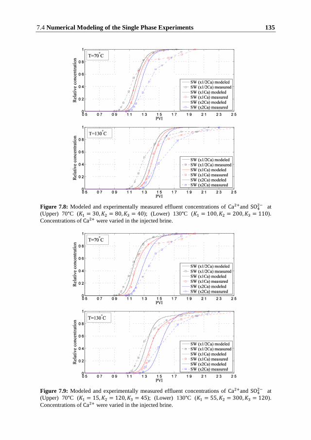
7.4 Numerical Modeling of the Single Phase Experiments 135

Figure 7.8: Modeled and experimentally measured effluent concentrations of Ca2+and SO42− at

(Upper) 70°C (𝐾1 = 30,𝐾2 = 80,𝐾3 = 40); (Lower) 130°C (𝐾1 = 100,𝐾2 = 200,𝐾3 = 110).

Concentrations of Ca2+ were varied in the injected brine.

Figure 7.9: Modeled and experimentally measured effluent concentrations of Ca2+and SO42− at

(Upper) 70°C (𝐾1 = 15,𝐾2 = 120,𝐾3 = 45); (Lower) 130°C (𝐾1 = 55,𝐾2 = 300,𝐾3 = 120).

Concentrations of Ca2+ were varied in the injected brine.

136 Analysis of Smart Waterflooding Experiments in Carbonates

Finally, we performed simulations to study competitive sorption of Ca2+and Mg2+ on the

surface in the absence of sulfate (experimental data of Zhang et al. [5]). Modeling of

competitive sorption of cations at 23°C is illustrated in Figure 7.10 and was performed with

𝐾1 = 20, 𝐾2 = 50. Our results indicate that a higher affinity of Ca2+ (𝐾2 > 𝐾1) should result

in an increase of the effluent concentration of Mg2+, which was not observed in the

experiment. This increase is not significant and is around 5-10% with our choice of

equilibrium constants.

Results of simulation for a similar experiment performed at 130°C are shown in Figure 7.11.

To achieve a significant increase in Ca2+ concentration we had to increase the ratio of the

equilibrium constants 𝐾1/𝐾2 to 5. Still, the discrepancy between model predictions and

experiment is high. Our results indicate that stronger adsorption of one of the cations in our

model will always result in an increase in the effluent concentration of the second cation. The

magnitude of this increase is proportional to the ratio of equilibrium constants.

Figure 7.10: Modeled and experimentally measured effluent concentrations of Ca2+, Mg2+ and

SCN− at 23°C. CF-M brine is injected in the chalk core initially saturated with ZP brine. 𝐾1 = 20,

𝐾2 = 50

Figure 7.11: Modeled and experimentally measured effluent concentrations of Ca2+, Mg2+ and

SCN− for 130°C . CF-M brine is injected in the chalk core initially saturated with ZP brine. 𝐾1 =1000, 𝐾2 = 200.

7.4 Numerical Modeling of the Single Phase Experiments 137

Results of simulation for a similar experiment performed at 130°C are shown in Figure 7.11.

In order to achieve a significant increase in Ca2+ concentration we had to increase the ratio

between equilibrium constants to 𝐾1/𝐾2 = 5. Still, the discrepancy between model

predictions and experiment is high. Our results indicate that stronger adsorption of one of the

cations in our model will always result in an increase of the effluent concentration of the

second cation. The magnitude of this increase is proportional to the ratio of equilibrium

constants.

In the discussion section, we pointed out that in this particular experiment Ca2+ is produced

from the core. In order to achieve this, it is required that the adsorbed Ca2+is initially present

on the surface. We accounted for this possibility by setting a low value of Ca2+ in the ZP

brine (0.573M NaCl): 𝑐𝑐𝑎 = 0.001 mol/l and a negative initial surface charge (to allow for

more calcium on the surface). In this case the increase in the effluent concentration of Ca2+

was more similar to the one observed in the experiments (Figure 7.12). However, the delay

between Ca2+ and Mg2+ breakthrough also significantly increased.

One of the possible explanations for inaccurate reproduction of these experimental data is the

simplifications introduced in the model by neglecting some of the surface complexes. In the

absence of sulfate, the complex > CaCO3− that we do not consider in this study would affect

the adsorption of calcium and magnesium. Because concentration of HCO3− in the injected

brines is low 𝑐𝐻𝐶𝑂3 = 0.002 mol/l, it is possible that equilibrium concentrations are achieved

after sufficient amount of brine is injected which is observed on the experimental curves

(Figure 7.11). Probably, full surface complexation model of carbonate surface described in

Chapter 3 should be used in order to provide a better match for this experiment.

The results presented in this section indicate that our model can qualitatively reproduce the

interaction between brines and the chalk surface. The match, however, is not accurate. In

order to improve the reliability of modeling, it is important to assess the repeatability of the

experiments, to know how broad the variation in the effluent concentrations curves is. Such

Figure 7.12: Modeled and experimentally measured effluent concentrations of Ca2+, Mg2+ and

SCN− for 130°C. CF-M brine is injected in the chalk core initially saturated with ZP brine with 𝑐𝑐𝑎 =

0.001 mol/l. 𝐾1 = 1000, 𝐾2 = 200.

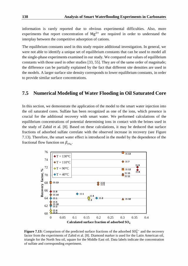
138 Analysis of Smart Waterflooding Experiments in Carbonates

information is rarely reported due to obvious experimental difficulties. Also, more

experiments that report concentration of Mg2+ are required in order to understand the

interplay between the competitive adsorption of cations.

The equilibrium constants used in this study require additional investigation. In general, we

were not able to identify a unique set of equilibrium constants that can be used to model all

the single-phase experiments examined in our study. We compared our values of equilibrium

constants with those used in other studies [33, 55]. They are of the same order of magnitude;

the difference can be partially explained by the fact that different site densities are used in

the models. A larger surface site density corresponds to lower equilibrium constants, in order

to provide similar surface concentrations.

7.5 Numerical Modeling of Water Flooding in Oil Saturated Core

In this section, we demonstrate the application of the model to the smart water injection into

the oil saturated cores. Sulfate has been recognized as one of the ions, which presence is

crucial for the additional recovery with smart water. We performed calculations of the

equilibrium concentrations of potential determining ions in contact with the brines used in

the study of Zahid et al. [8]. Based on these calculations, it may be deduced that surface

fractions of adsorbed sulfate correlate with the observed increase in recovery (see Figure

7.13). Therefore, the smart water effect is introduced in the model by the dependence of the

fractional flow function on 𝛽 𝑜 .

Figure 7.13: Comparison of the predicted surface fractions of the adsorbed SO42− and the recovery

factor from the experiments of Zahid et al. [8]. Diamond marker is used for the Latin American oil,

triangle for the North Sea oil, square for the Middle East oil. Data labels indicate the concentration

of sulfate and corresponding experiment.

3S 8

3S 9

0S 8

3S 15

3S 7

1S 61S 5

0S 14

0S 5

1S 4

1S 3

0S 40S 3

1S 2

1S 1

0S 2

0S 1

0S 10

3S 10

3S 11

0S 13

3S 12

3S 13

60

62

64

66

68

70

72

74

76

0 0.05 0.1 0.15 0.2 0.25 0.3 0.35 0.4

Rec

ov

ery

fa

cto

r, %

Calculated surface fraction of adsorbed SO4

T = 130°C

T = 110°C

T = 90°C

T = 40°C

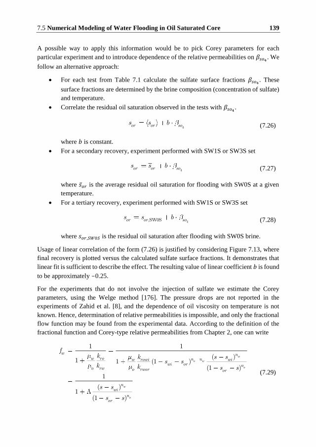
7.5 Numerical Modeling of Water Flooding in Oil Saturated Core 139

A possible way to apply this information would be to pick Corey parameters for each

particular experiment and to introduce dependence of the relative permeabilities on 𝛽 𝑜 . We

follow an alternative approach:

For each test from Table 7.1 calculate the sulfate surface fractions 𝛽 𝑜 . These

surface fractions are determined by the brine composition (concentration of sulfate)

and temperature.

Correlate the residual oil saturation observed in the tests with 𝛽 𝑜 .

4or or sos bs (7.26)

where 𝑏 is constant.

For a secondary recovery, experiment performed with SW1S or SW3S set

4or or sos s b (7.27)

where ��𝑜𝑟 is the average residual oil saturation for flooding with SW0S at a given

temperature.

For a tertiary recovery, experiment performed with SW1S or SW3S set

4,SW0Sor or sos s b (7.28)

where 𝑠𝑜𝑟,𝑆𝑊0𝑆 is the residual oil saturation after flooding with SW0S brine.

Usage of linear correlation of the form (7.26) is justified by considering Figure 7.13, where

final recovery is plotted versus the calculated sulfate surface fractions. It demonstrates that

linear fit is sufficient to describe the effect. The resulting value of linear coefficient 𝑏 is found

to be approximately -0.25.

For the experiments that do not involve the injection of sulfate we estimate the Corey

parameters, using the Welge method [176]. The pressure drops are not reported in the

experiments of Zahid et al. [8], and the dependence of oil viscosity on temperature is not

known. Hence, determination of relative permeabilities is impossible, and only the fractional

flow function may be found from the experimental data. According to the definition of the

fractional function and Corey-type relative permeabilities from Chapter 2, one can write

1 1

( )1 1 (1 )(1 )

1

( )1

(1 )

w

o w

o

w

o

w nw ro n nw rowi wi

wi or no rw o rwor or

nwi

nor

fk k s s

s sk k s s

s s

s s

(7.29)

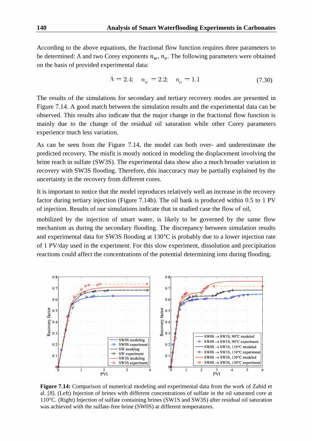
140 Analysis of Smart Waterflooding Experiments in Carbonates

According to the above equations, the fractional flow function requires three parameters to

be determined: Λ and two Corey exponents 𝑛𝑤, 𝑛𝑜. The following parameters were obtained

on the basis of provided experimental data:

2.4; 2.2; 1.1w on n (7.30)

The results of the simulations for secondary and tertiary recovery modes are presented in

Figure 7.14. A good match between the simulation results and the experimental data can be

observed. This results also indicate that the major change in the fractional flow function is

mainly due to the change of the residual oil saturation while other Corey parameters

experience much less variation.

As can be seen from the Figure 7.14, the model can both over- and underestimate the

predicted recovery. The misfit is mostly noticed in modeling the displacement involving the

brine reach in sulfate (SW3S). The experimental data show also a much broader variation in

recovery with SW3S flooding. Therefore, this inaccuracy may be partially explained by the

uncertainty in the recovery from different cores.

It is important to notice that the model reproduces relatively well an increase in the recovery

factor during tertiary injection (Figure 7.14b). The oil bank is produced within 0.5 to 1 PV

of injection. Results of our simulations indicate that in studied case the flow of oil,

mobilized by the injection of smart water, is likely to be governed by the same flow

mechanism as during the secondary flooding. The discrepancy between simulation results

and experimental data for SW3S flooding at 130°C is probably due to a lower injection rate

of 1 PV/day used in the experiment. For this slow experiment, dissolution and precipitation

reactions could affect the concentrations of the potential determining ions during flooding.

Figure 7.14: Comparison of numerical modeling and experimental data from the work of Zahid et

al. [8]. (Left) Injection of brines with different concentrations of sulfate in the oil saturated core at

110°C. (Right) Injection of sulfate containing brines (SW1S and SW3S) after residual oil saturation

was achieved with the sulfate-free brine (SW0S) at different temperatures.

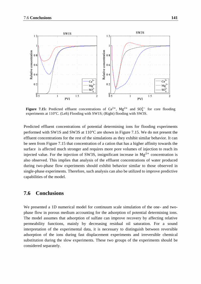
7.6 Conclusions 141

Predicted effluent concentrations of potential determining ions for flooding experiments

performed with SW1S and SW3S at 110°C are shown in Figure 7.15. We do not present the

effluent concentrations for the rest of the simulations as they exhibit similar behavior. It can

be seen from Figure 7.15 that concentration of a cation that has a higher affinity towards the

surface is affected much stronger and requires more pore volumes of injection to reach its

injected value. For the injection of SW3S, insignificant increase in Mg2+ concentration is

also observed. This implies that analysis of the effluent concentrations of water produced

during two-phase flow experiments should exhibit behavior similar to those observed in

single-phase experiments. Therefore, such analysis can also be utilized to improve predictive

capabilities of the model.

7.6 Conclusions

We presented a 1D numerical model for continuum scale simulation of the one- and two-

phase flow in porous medium accounting for the adsorption of potential determining ions.

The model assumes that adsorption of sulfate can improve recovery by affecting relative

permeability functions, mainly by decreasing residual oil saturation. For a sound

interpretation of the experimental data, it is necessary to distinguish between reversible

adsorption of the ions during fast displacement experiments and irreversible chemical

substitution during the slow experiments. These two groups of the experiments should be

considered separately.

Figure 7.15: Predicted effluent concentrations of Ca2+, Mg2+ and SO42− for core flooding

experiments at 110°C. (Left) Flooding with SW1S; (Right) flooding with SW3S.

142 Analysis of Smart Waterflooding Experiments in Carbonates

By comparison of the simulation results with the experimental data, we conclude that the

model is able to qualitatively reproduce single phase flow experiments. However, the

accuracy of data matching is low and further development of the model is required here.

Application of the model to the displacement of the oil by smart water predicts the increase

in oil recovery with a good match with the experimental data. The recovery is well correlated

with the presence of the sulfate ions. This indicates that the proposed simplified model

incorporates the recovery mechanisms that have been observed in the experiments. Further

development of the model is required in order to transfer the results onto the reservoir scale,

where slow chemical mechanisms may play a higher role.

The main conclusions that we draw from this study are:

1) The relative affinity of Ca2+ and Mg2+ changes with temperature. Some of the

experimental data suggest that Mg2+ will substitute Ca2+ on the surface at high

temperatures, while other data probably indicate that Mg2+ is inert towards the

surface. The results of the modeling suggest that adsorption of Ca2+ should be

stronger at high temperatures if sulfate is present.

2) At high temperatures, the model is not able to catch long-term decrease in Ca2+

concentration. The results of the modeling suggest that this should not be related to

the slower mechanisms of adsorption on the surface.

3) Concentrations of the potential determining ions in the water produced during two-

phase flow should exhibit behavior similar to those of the single-phase flow.

Therefore, we suggest that presenting data on the composition of the produced water

is essential for all the kinds of smart water flooding experiments.

4) Modeling of the two-phase flow flooding experiments indicates that incremental

recovery can be correlated to the change of the surface concentration of sulfate.

8 Conclusions and Future Work

Understanding of the factors that control the enhanced oil recovery during the smart

waterflooding in carbonate rocks is essential, since a considerable part of the hydrocarbon

reserves is contained in carbonate reservoirs. To improve this understanding, we addressed

several phenomena related to the smart water flooding, such as mineral dissolution, surface

chemistry of the carbonate rocks, and mechanisms that influence mobilization of trapped oil

and its transport. More specifically,

In Chapter 4 we presented a reactive transport model for the displacement problem

accounting for the fluid compressibility. Dissolution of the rock material was

affecting both the porosity/permeability of the rock and the density of the brine. It

was demonstrated that the velocity of the displacement front was slightly affected

by the non-additivity of the volumes under dissolution: the difference of individual

volumes of the mineral in solid and in solution. Contrary to our expectations, no

significant effect of non-additivity on the pressure was observed. We studied the

effect of the dissolution rate and observed that fast dissolution resembles formation

of wormholes with a significant change in porosity and permeability close to the

injection site. However, modeling in multiple dimensions is required to investigate

these effects more thoroughly.

In Chapter 5 we presented a micromodel for the two-phase flow in a single pore

body represented by an angular capillary. We performed numerical simulations to

study the effect of mutual presence and flow of the two fluids. The results of the

study indicate that presence of the water on the surface of the rock and in the corner

filaments of angular capillaries increases the velocity of the viscous flow of the oil

phase. We explain this phenomenon by the increased area of the moving boundary

of the oil-water interface. In the case of zero pressure drop in the oil phase, the flow

of oil may be induced by the action of viscous forces at the oil-water interface, which

appears to be a new mechanism for the transport of disconnected oil ganglia in

porous media. We found that the flow velocity of the oil ganglion is proportional to

the average flow velocity of the water present in the corner filaments.

In Chapter 6 we develop a macroscopic model to take into account the effects

associated with oil trapping and mobilization. We suggest that mobilization of

trapped oil ganglia may occur due to increasing wetness of the rock caused by the

presence of an active substance in the injected brine. According to the results of

Chapter 5, the flow of oil ganglia is slow as it is determined by the flow of the water

films. Results of numerical modeling of the tertiary recovery process indicate that

144 Conclusions and Future Work

production of oil ganglia may continue for a long time of injection of around 10 to

20 PVI. An important finding is that with the ganglia mobilization mechanism, the

oil bank travels behind the concentration front of the active substance. This result is

different from the predictions of the conventional model of chemical flooding,

where production of mobilized oil starts earlier than production of a chemical in the

effluent. Introduction of the non-equilibrium alteration of wettability and non-

instantaneous oil mobilization may be used to explain the delay observed in some

experiments, where mobilized oil is produced after several pore volumes of the

smart water injection.

In Chapter 7 we established a model to describe the interaction between an aqueous

solution and chalk during fast flooding experiments. Analysis of the available flow-

through experiments indicates that during flooding at high injection rates the brine-

rock interactions are determined by adsorption of the potential determining ions,

while both adsorption of ions and mineral reactions should be considered at low

injection rates and in spontaneous imbibition experiments. We estimated the

parameters that are used for the adsorption model by fitting the effluent

concentrations observed in the flow-through experiments. The computations

suggest that there is no evidence of usually assumed stronger adsorption of

magnesium ion compared to calcium at high temperatures. We combined the

adsorption model with the Buckley-Leverett model to perform simulations of the

two-phase flow experiments performed on the water-wet outcrop chalk [8].

Computation of the equilibrium surface composition demonstrated a correlation

between the concentration of the adsorbed sulfate and the ultimate recovery

observed in the experiments. Therefore, it might be suggested that a more

negatively charged surface of carbonate can be a factor that affects the recovery

efficiency without wettability modification.

Suggestions for Future Work

Considering the work and results presented in this thesis, it is clear that there are still major

uncertainties associated with the smart water flooding phenomena. The directions in which

the work can be extended include the following:

Oil-water and oil-rock interactions. More generally, this direction may be described

as the chemical theory of wettability in carbonates. Surface complexation models

[55] of the carbonate and the oil surfaces can be used to study the link between the

brine composition, concentrations of surface species and the polar oil components.

This will require introducing a number of poorly determined parameters, such as

equilibrium constants for the adsorption reactions at the oil-water interface and the

area of the interface. These constants are to be found in more refined experiments,

e.g. with the oil adhesion on the surface of calcite.

Conclusions and Future Work 145

A more realistic description of transport of the oil ganglia. We suggest that further

improvement of the oil ganglia model is required. The model should be extended to

account for the following possible processes: ganglia coalescence, retrapping and

transport in a pore network with varying capillary sizes. In order to make further

conclusions about the applicability of the model, it is also necessary to take into

account the end effects at the core facets.

The effect of mineral dissolution and solid precipitation on the concentrations of the

potential determining ions should be considered. The dissolution and precipitation

reactions play an important role at lower injection rates. Considering displacement

on the reservoir scale, both ion exchange on the surface and geochemical reactions

should be taken in account.

Inclusion of the capillary effects. Flooding in fractured carbonate reservoirs requires

accounting for both the viscous flow in the fractures and spontaneous imbibition in

the oil-wet porous matrix. For that reason, description of flooding in a core and in a

heterogeneous reservoir may be significantly different. Due to the slowness of

spontaneous imbibition process, this would require to consider the mineral

dissolution and precipitation reactions as suggested above.

Involvement of the migration of fines. It has been suggested that the fine migration

can be a reason for the smart water effects during injection of low salinity brine in

the sandstone and carbonate rocks. The effect of fines is associated with pore throat

blocking and diversion of the flow paths. The effect of fines migration cannot be

described adequately using only the macroscopic approach. However, it may be

studied within the framework of the deep bed filtration theory, which should

incorporate a physicochemical model of the interaction between the diluted aqueous

solution and the surface of the rock.

Geometry of the pore space should be described in more detail. It was observed that

smart water flooding in outcrop and reservoir cores can produce different results. If

the mineralogy of the rocks is similar, another reason that may cause the difference

should be found. One of the possibilities is to introduce the effect of the pore size

distribution, through a mesoscopic model based on the ensemble of pores [177].

This approach can be applied to describe a number of phenomena related to the

smart water effect and petrophysical experimental procedures including fines

migration, heterogeneous wettability and its alteration, the NMR measurements.

146 Conclusions and Future Work

Nomenclature

Abbreviation Description

AN Acid number

BC Boundary conditions

BN Base number

CBR Crude oil/brine/rock

EDL Electric double layer

EOR Enhanced oil recovery

ERA Equilibrium-rate-annihilation

FDM Finite difference method

FEM Finite element method

FIM Fully implicit method

FVM Finite volume method

FW Formation water

HS High salinity

HLL Harten, Lax, van Leer

IAP Ion activity product

IC Initial conditions

IFT Interfacial tension

IMPESC Implicit pressure, explicit saturations and compositions

LS Low salinity

LSW Low salinity waterflooding

MIE Multicomponent ion exchange

MPFA Multi-point flux approximation

MUSCL Monotonic upstream-centered scheme for conservation laws

OOIP Original oil in place

PVI Pore volumes injected

SI Saturation index

SPU Single-point upwind

SW Seawater

SWF Smart water flooding

TPFA Two-point flux approximation

USBM U.S. Bureau of Mines

WI Wettability index

148 Nomenclature

WAG Water alternating gas

Nomenclature Description

𝑖𝑗 Interface area between adjacent gridblocks, [m2]

Specific surface area of rock, [m2/l(core)]

Area of the capillary cross-section, [m2]

Area of the capillary cross-section occupied by phase 𝛼, [m2]

𝐶𝑚 Molar concentration of mineral species, [m2/l(core)]

𝑐𝑎 Molar concentration of species in phase, [m2/l]

𝑐∗ Molar concentration per bulk volume, [m2/l(core)]

��𝑃,𝛼 Compressibility of phase 𝛼 with regard to pressure

��𝑤𝑐,𝑎 Compressibility of brine with regard to composition

𝐶𝐸𝐶 Cation exchange capacity, [eq/m2]

𝐃𝑤 Diffusion tensor in water

Da Damköhler number

𝑑 Surface site density, [sites/nm2]

𝑓𝑤 Fractional flow function of water

ℱ Faraday’s constant, ℱ = 96485.3 𝐶/𝑚𝑜𝑙

𝐅 Flux term

𝐺 Shape factor

g Gravitational acceleration, 𝑔 = 9.81 m/s2

𝐻 Interpolation function

𝐻𝛼,𝑖𝑗 Fluid part of transmissibility for phase 𝛼 between adjacent gridblocks

ℎ Dimensionless thickness of the wetting film

𝐼 Ionic strength, [mol/l]

I Identity matrix

J Jacobian matrix

𝐾𝑛 Equilibrium constant for reaction 𝑛

𝑘 Scalar absolute permeability, [mDa]

𝐤 Absolute permeability tensor, [mDa]

𝑘𝑛 Rate constant for reaction 𝑛, [mol/m2/s]

𝑘𝑛𝑓, 𝑘𝑛𝑏 Forward and backward rate constant for reaction 𝑛, [mol/m2/s]

𝑘𝑟𝛼 Relative permeability of phase 𝛼

𝑘𝑟𝑤𝑜𝑟 , 𝑘𝑟𝑜𝑤𝑖 End point relative permeabilities for water and oil

𝐿 Distance between injection and production sites, [m]

l Length of capillary, [m]

𝑀𝑎 Molar weight, [kg/mol]

Nomenclature 149

�� Normal vector

𝑛 𝑝 Number of species

𝑛𝑟𝑒𝑎𝑐𝑡 Number of reactions

𝑁 Number of gridblocks

𝑛𝑤, 𝑛𝑜 Corey exponents

𝑃 Pressure, [Pa]

��𝑛 Rate of reaction 𝑛, [mol/m3/s]

𝑟ℎ Hydraulic radius, [m]

Q Convection source term

𝐪𝑖𝑛𝑗 Injection rate

𝑞𝛼 Volumetric flux of phase 𝛼 in capillary, [m3/s]

𝑅 Gas constant, 𝑅 = 8.31 J/K/mol

𝐒 Reactive source term

𝑠, 𝑠𝑤 Saturation of water

𝑠𝛼 Saturation of phase 𝛼

𝑠𝑜𝑟 Residual oil saturation

𝑠𝑤𝑖 Irreducible water saturation

𝑇 Absolute temperature, [K]

𝑇 Sorption capacity, [mol/m2]

𝑡 Time, [s]

𝑡𝐷 Dimensionless time

𝐔 Accumulation term

𝑢𝑡 Total flow velocity, [m/s]

𝑢𝛼 Flow velocity of phase 𝛼, [m/s]

𝑉𝑖 Volume of the gridblock, [𝑚3]

𝑣𝛼 Flow velocity of phase in capillary, [m/s]

𝐖 Primary variables

X𝑎 Chemical species

𝑥 Horizontal coordinate, [m]

𝑥𝐷 Dimensionless horizontal coordinate

𝑥 Spatial vector

𝑥 𝑖 Gridblock node vector

𝑥 𝑖𝑗 Internode vector

𝑦 Coordinate

𝑧 Coordinate along the capillary

𝑧𝑎 Charge of the species 𝑎

𝛼𝑟 Water-wet fraction of surface area

𝛽𝑎 Molar fractions of surface species

𝛽𝑎𝐺𝑇 Equivalent fractions of surface species

𝛽𝑖 Corner half-angles

Γ Henry adsorption constant

150 Nomenclature

Γ𝑖𝑗 Geometric part of transmissibility between adjacent gridblocks

Γ𝛼𝛽 Interface between phases 𝛼 and 𝛽 in capillary cross-section

𝛾𝑎 Activity coefficient of aqueous species

𝛾𝑚

𝛾𝑜𝑤 Interfacial tension between water and oil, [mN/m]

Δ𝑖 Limited slopes for the gridblock 𝑖

𝛿 Surface charge, [C/m2]

휀 Dielectric constant of water

휀0 Permittivity of free space, 휀0 = 8.854 × 10−12 F/m

𝜖𝑡𝑜𝑙 Tolerance

𝛼 Volumetric fraction of the porous medium occupied by phase 𝛼

𝜃 Contact angle

𝜅 Deposition rate, [s−1]

Mobility of the phase 𝛼

Λ𝑘 Eigenvalues of the matrix

𝜇𝛼 Viscosity of phase 𝛼, [cP]

𝜈𝑎𝑛 Stoichiometric coefficient for species 𝑎 in reaction 𝑛

Pressure gradient in phase 𝛼, [Pa/m]

Π Perimeter of capillary cross-section, [m]

𝜌𝛼 Density of phase 𝛼, [kg/m3]

𝜎𝑎 Surface molar concentration of species 𝑎, [mol/m2]

𝜏 Relaxation time

Υ𝑖𝑗 Transmissibility between adjacent gridblocks

𝜙 Porosity

𝜒 Electrostatic term

Surface potential, [V]

Ω𝑖 Gridblock

𝜕Ω𝑖 Boundary of the gridblock

𝜔𝑤 Wetting fluid saturation in capillary

Indexes

𝑎 Index for chemical species

𝑖, 𝑗 Indexes for gridblock

𝑖𝑛𝑗, J Index indicating injection

𝑚 Index for mineral species

𝑛 Index for time step

𝑜 Index for oil

𝑜𝑎 Index for oil cluster (“active” oil)

𝑜𝑔 Index for oil ganglia

Nomenclature 151

𝑜𝑢𝑡 Index indicating location at the outlet

𝑠 Index for solid phase

𝑤 Index for water

𝑤𝑎 Index for water cluster (“active” water)

𝑤𝑓 Index for water films

𝛼 Index for phases

𝛼 Index for surface species

0, I Index indicating the initial state

Bibliography

[1] H. Hermansen, G. Landa, J. Sylte, and L. Thomas, “Experiences after 10 years of

waterflooding the Ekofisk Field, Norway,” Journal of Petroleum Science and

Engineering, vol. 26, no. 1, pp. 11–18, 2000.

[2] T. Puntervold, S. Strand, R. Ellouz, T. Austad, et al., “Why is it Possible to Produce

Oil from the Ekofisk Field for Another 40 Years?,” in International Petroleum

Technology Conference, International Petroleum Technology Conference, 2014.

[3] T. Austad, S. Strand, E. Høgnesen, P. Zhang, et al., “Seawater as IOR fluid in

fractured chalk,” in SPE International Symposium on Oilfield Chemistry, Society of

Petroleum Engineers, 2005.

[4] S. Strand, T. Puntervold, and T. Austad, “Effect of temperature on enhanced oil

recovery from mixed-wet chalk cores by spontaneous imbibition and forced

displacement using seawater,” Energy & Fuels, vol. 22, no. 5, pp. 3222–3225, 2008.

[5] P. Zhang, M. T. Tweheyo, and T. Austad, “Wettability alteration and improved oil

recovery by spontaneous imbibition of seawater into chalk: Impact of the potential

determining ions Ca2+, Mg2+, and SO42-,” Colloids and Surfaces A: Physicochemical

and Engineering Aspects, vol. 301, no. 1, pp. 199–208, 2007.

[6] S. Strand, T. Austad, T. Puntervold, E. J. Høgnesen, M. Olsen, and S. M. F. Barstad,

““Smart water” for oil recovery from fractured limestone: a preliminary study,”

Energy & fuels, vol. 22, no. 5, pp. 3126–3133, 2008.

[7] S. J. Fathi, T. Austad, and S. Strand, ““Smart Water” as a Wettability Modifier in

Chalk: The Effect of Salinity and Ionic Composition,” Energy & fuels, vol. 24, no. 4,

pp. 2514–2519, 2010.

[8] A. Zahid, E. H. Stenby, A. A. Shapiro, et al., “Improved Oil Recovery in Chalk:

Wettability Alteration or Something Else?,” in SPE EUROPEC/EAGE Annual

Conference and Exhibition, Society of Petroleum Engineers, 2010.

[9] R. Gupta, G. G. Smith, L. Hu, T. Willingham, M. Lo Cascio, J. J. Shyeh, C. R.

Harris, et al., “Enhanced waterflood for carbonate reservoirs-impact of injection

water composition,” in SPE Middle East Oil and Gas Show and Conference, Society

of Petroleum Engineers, 2011.

[10] A. A. Yousef, S. H. Al-Saleh, A. Al-Kaabi, M. S. Al-Jawfi, et al., “Laboratory

investigation of the impact of injection-water salinity and ionic content on oil

recovery from carbonate reservoirs,” SPE Reservoir Evaluation & Engineering,

vol. 14, no. 05, pp. 578–593, 2011.

[11] O. Karoussi and A. A. Hamouda, “Imbibition of sulfate and magnesium ions into

carbonate rocks at elevated temperatures and their influence on wettability alteration

and oil recovery,” Energy & fuels, vol. 21, no. 4, pp. 2138–2146, 2007.

154 Bibliography

[12] J. Romanuka, J. Hofman, D. J. Ligthelm, B. Suijkerbuijk, F. Marcelis, S. Oedai,

N. Brussee, H. van der Linde, H. Aksulu, T. Austad, et al., “Low salinity eor in

carbonates,” in SPE Improved Oil Recovery Symposium, Society of Petroleum

Engineers, 2012.

[13] S. Strand, D. C. Standnes, and T. Austad, “Spontaneous imbibition of aqueous

surfactant solutions into neutral to oil-wet carbonate cores: Effects of brine salinity

and composition,” Energy & fuels, vol. 17, no. 5, pp. 1133–1144, 2003.

[14] P. Zhang, M. T. Tweheyo, and T. Austad, “Wettability alteration and improved oil

recovery in chalk: The effect of calcium in the presence of sulfate,” Energy & fuels,

vol. 20, no. 5, pp. 2056–2062, 2006.

[15] A. RezaeiDoust, T. Puntervold, S. Strand, and T. Austad, “Smart water as wettability

modifier in carbonate and sandstone: A discussion of similarities/differences in the

chemical mechanisms,” Energy & fuels, vol. 23, no. 9, pp. 4479–4485, 2009.

[16] H. H. Al-Attar, M. Y. Mahmoud, A. Y. Zekri, R. Almehaideb, and M. Ghannam,

“Low-salinity flooding in a selected carbonate reservoir: experimental approach,”

Journal of Petroleum Exploration and Production Technology, vol. 3, no. 2,

pp. 139–149, 2013.

[17] E. J. Hognesen, S. Strand, T. Austad, et al., “Waterflooding of preferential oil-wet

carbonates: Oil recovery related to reservoir temperature and brine composition,” in

SPE Europec/EAGE Annual Conference, Society of Petroleum Engineers, 2005.

[18] T. Puntervold, S. Strand, and T. Austad, “Water flooding of carbonate reservoirs:

Effects of a model base and natural crude oil bases on chalk wettability,” Energy &

fuels, vol. 21, no. 3, pp. 1606–1616, 2007.

[19] M. T. Tweheyo, P. Zhang, T. Austad, et al., “The effects of temperature and

potential determining ions present in seawater on oil recovery from fractured

carbonates,” in SPE/DOE Symposium on Improved Oil Recovery, Society of

Petroleum Engineers, 2006.

[20] S. J. Fathi, T. Austad, and S. Strand, “Water-based enhanced oil recovery (EOR) by

“smart water”: Optimal ionic composition for EOR in carbonates,” Energy & fuels,

vol. 25, no. 11, pp. 5173–5179, 2011.

[21] A. Zahid, A. A. Shapiro, A. Skauge, et al., “Experimental Studies of Low Salinity

Water Flooding Carbonate: A New Promising Approach,” in SPE EOR Conference

at Oil and Gas West Asia, Society of Petroleum Engineers, 2012.

[22] H. S. Al-Hadhrami, M. J. Blunt, et al., “Thermally induced wettability alteration to

improve oil recovery in fractured reservoirs,” in SPE/DOE Improved Oil Recovery

Symposium, Society of Petroleum Engineers, 2000.

[23] L. Yu, D. C. Standnes, and S. M. Skjæveland, “Wettability alteration of chalk by

sulphate containing water, monitored by contact angle measurement,” in SCA2007-

01, presented at the International Symposium of the Society of Core Analysis,

Calgary, 2007.

[24] A. Lager, K. Webb, C. Black, M. Singleton, K. Sorbie, et al., “Low Salinity Oil

Recovery-An Experimental Investigation,” Petrophysics, vol. 49, no. 01, 2008.

[25] A. A. Yousef, S. Al-Saleh, M. S. Al-Jawfi, et al., “Improved/enhanced oil recovery

from carbonate reservoirs by tuning injection water salinity and ionic content,” in

SPE Improved Oil Recovery Symposium, Society of Petroleum Engineers, 2012.

Bibliography 155

[26] S. J. Fathi, T. Austad, S. Strand, and T. Puntervold, “Wettability alteration in

carbonates: The effect of water-soluble carboxylic acids in crude oil,” Energy &

Fuels, vol. 24, no. 5, pp. 2974–2979, 2010.

[27] A. Zahid, Smart Waterflooding in Carbonate Reservoirs. PhD thesis, Technical

University of Denmark, 2012.

[28] K. H. Chakravarty, P. L. Fosbøl, K. Thomsen, et al., “Brine Crude Oil Interactions

at the Oil-Water Interface,,” in SPE International Symposium on Oilfield Chemistry,

Society of Petroleum Engineers, 2015.

[29] J. Benicek, “Application of Emulsion Formed Enzymes for Enhanced Oil

Recovery,” Master’s thesis, Technical University of Denmark, 2015.

[30] A. Zahid, A. Shapiro, E. H. Stenby, and W. Yan, “Managing injected water

composition to improve oil recovery: A case study of North Sea chalk reservoirs,”

Energy & Fuels, vol. 26, no. 6, pp. 3407–3415, 2012.

[31] I. Fjelde and S. Aasen, “Improved spontaneous imbibition of water in reservoir

chalks,” in IOR 2009-15th European Symposium on Improved Oil Recovery, 2009.

[32] S. Strand, E. J. Høgnesen, and T. Austad, “Wettability alteration of carbonates—

Effects of potential determining ions (Ca2+ and SO42-) and temperature,” Colloids

and Surfaces A: Physicochemical and Engineering Aspects, vol. 275, no. 1, pp. 1–

10, 2006.

[33] A. Hiorth, L. Cathles, and M. Madland, “The impact of pore water chemistry on

carbonate surface charge and oil wettability,” Transport in porous media, vol. 85,

no. 1, pp. 1–21, 2010.

[34] M. Madland, B. Zangiabadi, R. Korsnes, S. Evje, L. Cathles, T. Kristiansen, and

A. Hiorth, “Rock Fluid Interactions in Chalk with MgCl2 and Na2Cl4 Brines with

Equal Ionic Strength,” in 15th European Symposium on Improved Oil Recovery,

2009.

[35] G.-Q. Tang and N. R. Morrow, “Influence of brine composition and fines migration

on crude oil/brine/rock interactions and oil recovery,” Journal of Petroleum Science

and Engineering, vol. 24, no. 2, pp. 99–111, 1999.

[36] H. Pu, X. Xie, P. Yin, N. R. Morrow, et al., “Low-salinity waterflooding and mineral

dissolution,” in SPE Annual Technical Conference and Exhibition, Society of

Petroleum Engineers, 2010.

[37] W. Winoto, N. Loahardjo, S. X. Xie, P. Yin, N. R. Morrow, et al., “Secondary and

tertiary recovery of crude oil from outcrop and reservoir rocks by low salinity

waterflooding,” in SPE Improved Oil Recovery Symposium, Society of Petroleum

Engineers, 2012.

[38] K. H. Chakravarty, P. L. Fosbøl, K. Thomsen, et al., “Importance of Fines in Smart

Water Enhanced Oil Recovery (SmW-EOR) for Chalk Outcrops,” in EUROPEC

2015, Society of Petroleum Engineers, 2015.

[39] D. J. Ligthelm, J. Gronsveld, J. Hofman, N. Brussee, F. Marcelis, H. van der Linde,

et al., “Novel waterflooding strategy by manipulation of injection brine

composition.,” in EUROPEC/EAGE Conference and Exhibition, Society of

Petroleum Engineers, 2009.

[40] G. G. Bernard et al., “Effect of floodwater salinity on recovery of oil from cores

containing clays,” in SPE California Regional Meeting, Society of Petroleum

Engineers, 1967.

156 Bibliography

[41] P. P. Jadhunandan, Effects of brine composition, crude oil, and aging conditions on

wettability and oil recovery. Department of Petroleum Engineering, New Mexico

Institute of Mining & Technology, 1990.

[42] P. Jadhunandan and N. Morrow, “Spontaneous imbibition of water by crude

oil/brine/rock systems,” In Situ;(United States), vol. 15, no. 4, 1991.

[43] P. Jadhunandan, N. R. Morrow, et al., “Effect of wettability on waterflood recovery

for crude-oil/brine/rock systems,” SPE reservoir engineering, vol. 10, no. 01,

pp. 40–46, 1995.

[44] G. Tang, N. R. Morrow, et al., “Salinity, temperature, oil composition, and oil

recovery by waterflooding,” SPE Reservoir Engineering, vol. 12, no. 04, pp. 269–

276, 1997.

[45] P. McGuire, J. Chatham, F. Paskvan, D. Sommer, F. Carini, et al., “Low salinity oil

recovery: An exciting new EOR opportunity for Alaska’s North Slope,” in SPE

Western Regional Meeting, Society of Petroleum Engineers, 2005.

[46] G. R. Jerauld, K. J. Webb, C.-Y. Lin, J. C. Seccombe, et al., “Modeling low-salinity

waterflooding,” SPE Reservoir Evaluation & Engineering, vol. 11, no. 06, pp. 1–

000, 2008.

[47] H. Mahani, T. Sorop, D. J. Ligthelm, D. Brooks, P. Vledder, F. Mozahem, Y. Ali,

et al., “Analysis of field responses to low-salinity waterflooding in secondary and

tertiary mode in Syria,” in SPE EUROPEC/EAGE Annual Conference and

Exhibition, Society of Petroleum Engineers, 2011.

[48] A. Omekeh, S. Evje, I. Fjelde, and H. A. Friis, “Experimental and modeling

investigation of ion exchange during low salinity waterflooding,” in SCA 2011-038

presented at the International Symposium of the Society of Core Analysts, Austin,

Texas, USA, pp. 18–21, 2011.

[49] A. V. Omekeh, A, S. Evje, S., and H. A. Friis, H. A.Riis, “Modeling of low salinity

effects in sandstone oil rocks,” International Journal of Numerical Analysis and

Modelling, vol. 1, no. 1, pp. 1–18, 2012.

[50] C. T. Q. Dang, L. X. Nghiem, Z. J. Chen, Q. P. Nguyen, et al., “Modeling low

salinity waterflooding: ion exchange, geochemistry and wettability alteration,” in

SPE Annual Technical Conference and Exhibition, Society of Petroleum Engineers,

2013.

[51] C. T. Dang, L. X. Nghiem, Z. Chen, Q. P. Nguyen, N. T. Nguyen, et al., “State-of-

the art low salinity waterflooding for enhanced oil recovery,” in SPE Asia Pacific

Oil and Gas Conference and Exhibition, Society of Petroleum Engineers, 2013.

[52] A. Hiorth, E. Jettestuen, L. M. Cathles, R. I. Korsnes, and M. V. Madland, “A fully

Coupled Geochemical Model with a Pore Scale Lattice Boltzmann Simulator-

Principles and First Results,” SCA, 2010.

[53] S. Evje and A. Hiorth, “A mathematical model for dynamic wettability alteration

controlled by water-rock chemistry,” NHM, vol. 5, no. 2, pp. 217–256, 2010.

[54] S. Strand, D. Standnes, and T. Austad, “New wettability test for chalk based on

chromatographic separation of SCN- and SO42-,” Journal of Petroleum Science and

Engineering, vol. 52, no. 1, pp. 187–197, 2006.

[55] P. V. Brady, J. L. Krumhansl, P. E. Mariner, et al., “Surface complexation modeling

for improved oil recovery,” in SPE Improved Oil Recovery Symposium, Society of

Petroleum Engineers, 2012.

Bibliography 157

[56] Y. Zaretskiy, Towards modelling physical and chemical effects during wettability

alteration in carbonates at pore and continuum scales. PhD thesis, Heriot-Watt

University, 2012.

[57] M. Madland, A. Hiorth, E. Omdal, M. Megawati, T. Hildebrand-Habel, R. Korsnes,

S. Evje, and L. Cathles, “Chemical alterations induced by rock–fluid interactions

when injecting brines in high porosity chalks,” Transport in porous media, vol. 87,

no. 3, pp. 679–702, 2011.

[58] R. Salathiel et al., “Oil recovery by surface film drainage in mixed-wettability

rocks,” Journal of Petroleum Technology, vol. 25, no. 10, pp. 1–216, 1973.

[59] W. G. Anderson, “Wettability literature survey-Part 1: Rock/oil/brine interactions

and the effects of core handling on wettability,” J. Pet. Technol.;(United States),

vol. 38, no. 11, 1986.

[60] R. Johnson and R. Dettre, “Wettability and contact angles,” Surface and colloid

science, vol. 2, pp. 85–153, 1969.

[61] W. Abdallah, J. S. Buckley, A. Carnegie, J. Edwards, B. Herold, E. Fordham,

A. Graue, T. Habashy, N. Seleznev, C. Signer, H. Hussain, B. Montaron, and

M. Ziauddin, “Fundamentals of wettability,” Oilfield Review, 2007.

[62] M. Leverett et al., “Capillary behavior in porous solids,” Transactions of the AIME,

vol. 142, no. 01, pp. 152–169, 1941.

[63] E. C. Donaldson, R. D. Thomas, P. B. Lorenz, et al., “Wettability determination and

its effect on recovery efficiency,” Society of Petroleum Engineers Journal, vol. 9,

no. 01, pp. 13–20, 1969.

[64] N. R. Morrow, Interfacial phenomena in petroleum recovery. CRC Press, 1990.

[65] W. Anderson et al., “Wettability literature survey-part 2: Wettability measurement,”

Journal of Petroleum Technology, vol. 38, no. 11, pp. 1–246, 1986.

[66] F. F. Craig, The reservoir engineering aspects of waterflooding. Richardson, TX:

Henry L. Doherty Memorial Fund of AIME, Society of Petroleum Engineers, 1993.

[67] J. Roof et al., “Snap-off of oil droplets in water-wet pores,” Society of Petroleum

Engineers Journal, vol. 10, no. 01, pp. 85–90, 1970.

[68] I. Chatzis, N. R. Morrow, H. T. Lim, et al., “Magnitude and detailed structure of

residual oil saturation,” Society of Petroleum Engineers Journal, vol. 23, no. 02,

pp. 311–326, 1983.

[69] W. G. Anderson et al., “Wettability literature survey-part 6: the effects of wettability

on waterflooding,” Journal of Petroleum Technology, vol. 39, no. 12, pp. 1–605,

1987.

[70] L. P. Dake, Fundamentals of reservoir engineering. Elsevier, 1983.

[71] L. Plummer, T. Wigley, and D. Parkhurst, “The kinetics of calcite dissolution in

CO2-water systems at 5 degrees to 60 degrees C and 0.0 to 1.0 atm CO2,” American

Journal of Science, vol. 278, no. 2, pp. 179–216, 1978.

[72] C. A. J. Appelo and D. Postma, Geochemistry, groundwater and pollution. CRC

press, 2005.

[73] O. S. Pokrovsky, S. V. Golubev, J. Schott, and A. Castillo, “Calcite, dolomite and

magnesite dissolution kinetics in aqueous solutions at acid to circumneutral pH, 25

to 150 C and 1 to 55 atm pCO2: new constraints on CO2 sequestration in sedimentary

basins,” Chemical geology, vol. 265, no. 1, pp. 20–32, 2009.

158 Bibliography

[74] D. Hasson and J. Zahavi, “Mechanism of calcium sulfate scale deposition on heat

transfer surfaces,” Industrial & Engineering Chemistry Fundamentals, vol. 9, no. 1,

pp. 1–10, 1970.

[75] C. M. Bethke, Geochemical and biogeochemical reaction modeling. Cambridge

University Press, 2007.

[76] R. S. Arvidson, I. E. Ertan, J. E. Amonette, and A. Luttge, “Variation in calcite

dissolution rates:: A fundamental problem?,” Geochimica et cosmochimica acta,

vol. 67, no. 9, pp. 1623–1634, 2003.

[77] J. A. Davis and D. Kent, “Surface complexation modeling in aqueous

geochemistry,” Reviews in Mineralogy and Geochemistry, vol. 23, no. 1, pp. 177–

260, 1990.

[78] P. A. Domenico and F. W. Schwartz, Physical and chemical hydrogeology, vol. 44.

Wiley New York, 1998.

[79] A. W. Adamson, A. P. Gast, et al., Physical chemistry of surfaces. Interscience

publishers New York, 1967.

[80] W. Stumm and J. Morgan, “Aquatic chemistry, chemical equilibra and rates in

natural waters,” Environmental Science and Technology Series, 1996.

[81] G. Sposito, The chemistry of soils. Oxford university press, 2008.

[82] J. N. Israelachvili, Intermolecular and surface forces: revised third edition.

Academic press, 2011.

[83] D. A. Dzombak and F. M. Morel, Surface complexation modeling: hydrous ferric

oxide. John Wiley & Sons, 1990.

[84] D. C. Grahame, “The electrical double layer and the theory of electrocapillarity,”

Chemical reviews, vol. 41, no. 3, pp. 441–501, 1947.

[85] S. E. Buckley, M. Leverett, et al., “Mechanism of fluid displacement in sands,”

Transactions of the AIME, vol. 146, no. 01, pp. 107–116, 1942.

[86] G. A. Pope et al., “The application of fractional flow theory to enhanced oil

recovery,” Society of Petroleum Engineers Journal, vol. 20, no. 03, pp. 191–205,

1980.

[87] R. Brooks and T. Corey, “Hydraulic properties of porous media,” 1964.

[88] L. W. Lake, Enhanced oil recovery. Old Tappan, NJ; Prentice Hall Inc., 1989.

[89] H. J. Welge et al., “A simplified method for computing oil recovery by gas or water

drive,” Journal of Petroleum Technology, vol. 4, no. 04, pp. 91–98, 1952.

[90] J. S. Archer and C. G. Wall, Petroleum engineering: principles and practice.

Springer Science & Business Media, 2012.

[91] P. Donnez, Essentials of reservoir engineering, vol. 2. TECHNIP OPHRYS

EDITIONS, 2012.

[92] P. Bedrikovetsky, Mathematical theory of oil and gas recovery: with applications

to ex-USSR oil and gas fields, vol. 4. Springer Science & Business Media, 1993.

[93] J. Sheng, Modern chemical enhanced oil recovery: theory and practice. Gulf

Professional Publishing, 2010.

[94] R. Courant and K. O. Friedrichs, Supersonic flow and shock waves, vol. 21. Springer

Science & Business Media, 1999.

Bibliography 159

[95] U. Korsbech, H. Aage, K. Hedegaard, B. L. Andersen, N. Springer, et al.,

“Measuring and modeling the displacement of connate water in chalk core plugs

during water injection,” SPE Reservoir Evaluation & Engineering, vol. 9, no. 03,

pp. 259–265, 2006.

[96] J. Patton, K. Coats, G. Colegrove, et al., “Prediction of polymer flood performance,”

Society of Petroleum Engineers Journal, vol. 11, no. 01, pp. 72–84, 1971.

[97] W. Foster et al., “A low-tension waterflooding process,” Journal of Petroleum

Technology, vol. 25, no. 02, pp. 205–210, 1973.

[98] R. Larson et al., “Analysis of the physical mechanisms in surfactant flooding,”

Society of Petroleum Engineers Journal, vol. 18, no. 01, pp. 42–58, 1978.

[99] E. F. Toro, Riemann solvers and numerical methods for fluid dynamics: a practical

introduction. Springer Science & Business Media, 2009.

[100] L. Nghiem, P. Sammon, J. Grabenstetter, H. Ohkuma, et al., “Modeling CO2 storage

in aquifers with a fully-coupled geochemical EOS compositional simulator,” in

SPE/DOE symposium on improved oil recovery, Society of Petroleum Engineers,

2004.

[101] C. Hirsch, Numerical Computation of Internal and External Flows: The

Fundamentals of Computational Fluid Dynamics, vol. 1. Butterworth-Heinemann,

2007.

[102] Z. Chen, Reservoir simulation: mathematical techniques in oil recovery, vol. 77.

SIAM, 2007.

[103] R. J. LeVeque, Finite difference methods for ordinary and partial differential

equations: steady-state and time-dependent problems, vol. 98. Siam, 2007.

[104] H. K. Versteeg and W. Malalasekera, An introduction to computational fluid

dynamics: the finite volume method. Pearson Education, 2007.

[105] K. Aziz and A. Settari, Petroleum reservoir simulation. Chapman & Hall, 1979.

[106] J. H. Abou-Kassem, S. Farouq-Ali, and M. R. Islam, Petroleum Reservoir

Simulations. Elsevier, 2013.

[107] J. Cordazzo, C. R. Maliska, and A. Silva, “Interblock transmissibility calculation

analysis for petroleum reservoir simulation,” in 2nd Meeting on Reservoir

Simulation, Universidad Argentina de la Empresa, Buenos Aires, Argentina,

November, pp. 5–6, 2002.

[108] G. L. Chierici, Principles of petroleum reservoir engineering, vol. 2. Springer

Science & Business Media, 2012.

[109] L. F. Shampine, Numerical solution of ordinary differential equations, vol. 4. CRC

Press, 1994.

[110] J. M. Ortega and W. C. Rheinboldt, Iterative solution of nonlinear equations in

several variables, vol. 30. Siam, 1970.

[111] J. J. Moré, B. S. Garbow, and K. E. Hillstrom, “User guide for MINPACK-1,” tech.

rep., CM-P00068642, 1980.

[112] D. E. van Odyck, S. Lovett, F. Monmont, and N. Nikiforakis, “An efficient shock

capturing scheme for multicomponent multiphase thermal flow in porous media,”

in Proceedings of the Royal Society of London A: Mathematical, Physical and

Engineering Sciences, p. rspa20120152, The Royal Society, 2012.

160 Bibliography

[113] M. B. Alotaibi, H. A. Nasr-El-Din, et al., “Chemistry of injection water and its

impact on oil recovery in carbonate and clastics formations,” in SPE international

symposium on oilfield chemistry, Society of Petroleum Engineers, 2009.

[114] T. Austad, S. Shariatpanahi, S. Strand, C. Black, and K. Webb, “Conditions for a

low-salinity enhanced oil recovery (EOR) effect in carbonate oil reservoirs,” Energy

& fuels, vol. 26, no. 1, pp. 569–575, 2011.

[115] A. C. Lasaga, “Chemical kinetics of water-rock interactions,” Journal of

Geophysical Research: Solid Earth (1978–2012), vol. 89, no. B6, pp. 4009–4025,

1984.

[116] O. Singurindy and B. Berkowitz, “Evolution of hydraulic conductivity by

precipitation and dissolution in carbonate rock,” Water Resources Research, vol. 39,

no. 1, 2003.

[117] P. G. Bedrikovetsky, E. J. Mackay, R. M. Silva, F. M. Patricio, and F. F. Rosário,

“Produced water re-injection with seawater treated by sulphate reduction plant:

Injectivity decline, analytical model,” Journal of Petroleum Science and

Engineering, vol. 68, no. 1, pp. 19–28, 2009.

[118] P. Bedrikovetsky, R. M. Silva, J. S. Daher, J. A. Gomes, and V. C. Amorim, “Well-

data-based prediction of productivity decline due to sulphate scaling,” Journal of

Petroleum Science and Engineering, vol. 68, no. 1, pp. 60–70, 2009.

[119] S. Houston, B. Yardley, P. Smalley, and I. Collins, “Precipitation and dissolution of

minerals during waterflooding of a North Sea oil field,” paper SPE, vol. 100603,

2006.

[120] E. Aharonov, M. Spiegelman, and P. Kelemen, “Three-dimensional flow and

reaction in porous media: Implications for the Earth’s mantle and sedimentary

basins,” JOURNAL OF GEOPHYSICAL RESEARCH-ALL SERIES-, vol. 102,

pp. 14–821, 1997.

[121] J. Spivey, W. McCain Jr, R. North, et al., “Estimating density, formation volume

factor, compressibility, methane solubility, and viscosity for oilfield brines at

temperatures from 0 to 275C, pressures to 200 MPa, and salinities to 5.7 mole/kg,”

Journal of Canadian Petroleum Technology, vol. 43, no. 07, 2004.

[122] E. J. Lam, M. N. Alvarez, M. E. Galvez, and E. B. Alvarez, “A model for calculating

the density of aqueous multicomponent electrolyte solutions,” Journal of the

Chilean Chemical Society, vol. 53, no. 1, pp. 1393–1398, 2008.

[123] J. Rubin, “Transport of reacting solutes in porous media: Relation between

mathematical nature of problem formulation and chemical nature of reactions,”

Water resources research, vol. 19, no. 5, pp. 1231–1252, 1983.

[124] A. Settari, F. Mourits, et al., “A coupled reservoir and geomechanical simulation

system,” Spe Journal, vol. 3, no. 03, pp. 219–226, 1998.

[125] R. P. Chapuis and M. Aubertin, Predicting the coefficient of permeability of soils

using the Kozeny-Carman equation. École polytechnique de Montréal, 2003.

[126] M. M. Alam, I. L. Fabricius, and M. Prasad, “Permeability prediction in chalks,”

AAPG bulletin, vol. 95, no. 11, pp. 1991–2014, 2011.

[127] M. J. Blunt, “Flow in porous media—pore-network models and multiphase flow,”

Current opinion in colloid & interface science, vol. 6, no. 3, pp. 197–207, 2001.

Bibliography 161

[128] P. H. Valvatne, Predictive pore-scale modelling of multiphase flow. PhD thesis,

Imperial College London, 2004.

[129] P. H. Valvatne, M. Piri, X. Lopez, and M. J. Blunt, “Predictive pore-scale modeling

of single and multiphase flow,” in Upscaling Multiphase Flow in Porous Media,

pp. 23–41, Springer, 2005.

[130] T. W. Patzek et al., “Verification of a complete pore network simulator of drainage

and imbibition,” in SPE/DOE Improved Oil Recovery Symposium, Society of

Petroleum Engineers, 2000.

[131] T. Patzek and J. Kristensen, “Shape factor correlations of hydraulic conductance in

noncircular capillaries: II. Two-phase creeping flow,” Journal of colloid and

interface science, vol. 236, no. 2, pp. 305–317, 2001.

[132] T. Patzek and D. Silin, “Shape factor and hydraulic conductance in noncircular

capillaries: I. One-phase creeping flow,” Journal of colloid and interface science,

vol. 236, no. 2, pp. 295–304, 2001.

[133] A. Ryazanov, M. Van Dijke, and K. Sorbie, “Two-phase pore-network modelling:

existence of oil layers during water invasion,” Transport in Porous Media, vol. 80,

no. 1, pp. 79–99, 2009.

[134] P.-E. Oren, S. Bakke, O. J. Arntzen, et al., “Extending predictive capabilities to

network models,” SPE Journal, vol. 3, no. 04, pp. 324–336, 1998.

[135] W. Rose, “Coupling coefficients for two-phase flow in pore spaces of simple

geometry,” Transport in Porous Media, vol. 5, no. 1, pp. 97–102, 1990.

[136] A. A. Shapiro, “Two-Phase Immiscible Flows in Porous Media: The Mesocopic

Maxwell–Stefan Approach,” Transport in Porous Media, vol. 107, no. 2, pp. 335–

363, 2015.

[137] F. U. Guide, Version 5.0, PDE Solutions, 2005.

[138] A. Payatakes, “Dynamics of oil ganglia during immiscible displacement in water-

wet porous media,” Annual Review of Fluid Mechanics, vol. 14, no. 1, pp. 365–393,

1982.

[139] P. Bedrikovetsky et al., “A new mathematical model for EOR displacements

honouring oil ganglia,” in SPE Annual Technical Conference and Exhibition,

Society of Petroleum Engineers, 1997.

[140] D. W. Green, Enhanced oil recovery. 1998.

[141] M. Gray, A. Yeung, J. Foght, H. W. Yarranton, et al., “Potential microbial enhanced

oil recovery processes: a critical analysis,” in SPE Annual Technical Conference

and Exhibition, Society of Petroleum Engineers, 2008.

[142] A. Halim, A. Shapiro, A. E. Lantz, and S. M. Nielsen, “Experimental study of

bacterial penetration into chalk rock: mechanisms and effect on permeability,”

Transport in porous media, vol. 101, no. 1, pp. 1–15, 2014.

[143] T. Austad, “Water-Based EOR in Carbonates and Sandstones: New Chemical

Understanding of the EOR Potential Using Smart Water,” Enhanced Oil Recovery

Field Case Studies, pp. 301–335, 2013.

[144] R. Lenormand, C. Zarcone, and A. Sarr, “Mechanisms of the displacement of one

fluid by another in a network of capillary ducts,” Journal of Fluid Mechanics,

vol. 135, pp. 337–353, 1983.

162 Bibliography

[145] E. J. Spiteri, R. Juanes, M. J. Blunt, F. M. Orr, et al., “A new model of trapping and

relative permeability hysteresis for all wettability characteristics,” Spe Journal,

vol. 13, no. 03, pp. 277–288, 2008.

[146] C. H. Pentland, E. Itsekiri, S. Al-Mansoori, S. Iglauer, B. Bijeljic, M. J. Blunt, et al.,

“Measurement of nonwetting-phase trapping in sandpacks,” Spe Journal, vol. 15,

no. 02, pp. 274–281, 2010.

[147] H. Princen, “Capillary phenomena in assemblies of parallel cylinders: II. Capillary

rise in systems with more than two cylinders,” Journal of Colloid and Interface

Science, vol. 30, no. 3, pp. 359–371, 1969.

[148] A. V. Ryazanov, M. I. van Dijke, K. S. Sorbie, et al., “Pore-network prediction of

residual oil saturation based on oil layer drainage in mixed-wet systems,” in SPE

Improved Oil Recovery Symposium, Society of Petroleum Engineers, 2010.

[149] N. R. Morrow et al., “Wettability and its effect on oil recovery,” Journal of

Petroleum Technology, vol. 42, no. 12, pp. 1–476, 1990.

[150] X. Zhao, M. J. Blunt, and J. Yao, “Pore-scale modeling: Effects of wettability on

waterflood oil recovery,” Journal of Petroleum Science and Engineering, vol. 71,

no. 3, pp. 169–178, 2010.

[151] K. P. Abeysinghe, I. Fjelde, A. Lohne, et al., “Dependency of Remaining Oil

Saturation on Wettability and Capillary Number,” in SPE Saudi Arabia Section

Technical Symposium and Exhibition, Society of Petroleum Engineers, 2012.

[152] K. A. Rezaei Gomari, O. Karoussi, A. A. Hamouda, et al., “Mechanistic study of

interaction between water and carbonate rocks for enhancing oil recovery,” in SPE

Europec/EAGE Annual Conference and Exhibition, Society of Petroleum

Engineers, 2006.

[153] M. B. Alotaibi, R. Azmy, H. A. Nasr-El-Din, et al., “Wettability challenges in

carbonate reservoirs,” in SPE Improved Oil Recovery Symposium, Society of

Petroleum Engineers, 2010.

[154] A. Seethepalli, B. Adibhatla, K. Mohanty, et al., “Wettability alteration during

surfactant flooding of carbonate reservoirs,” in SPE/DOE Symposium on Improved

Oil Recovery, Society of Petroleum Engineers, 2004.

[155] D. C. Standnes and T. Austad, “Wettability alteration in chalk: 2. Mechanism for

wettability alteration from oil-wet to water-wet using surfactants,” Journal of

Petroleum Science and Engineering, vol. 28, no. 3, pp. 123–143, 2000.

[156] H. Nasiri, K. Spildo, and A. Skauge, “Use of enzymes to improve waterflood

Performance,” in International Symposium of the Society of Core Analysts, pp. 27–

30, 2009.

[157] R. Sen, “Biotechnology in petroleum recovery: the microbial EOR,” Progress in

Energy and Combustion Science, vol. 34, no. 6, pp. 714–724, 2008.

[158] B. Soraya, C. Malick, C. Philippe, H. J. Bertin, G. Hamon, et al., “Oil recovery by

low-salinity brine injection: Laboratory results on outcrop and reservoir cores,” in

SPE Annual Technical Conference and Exhibition, Society of Petroleum Engineers,

2009.

[159] N. Hadia, H. H. Lehne, K. G. Kumar, K. A. Selboe, F. Å. Stensen, O. Torsater, et al.,

“Laboratory Investigation of Low Salinity Waterflooding on Reservoir Rock

Samples from the Froy Field,” in SPE Middle East Oil and Gas Show and

Conference, Society of Petroleum Engineers, 2011.

Bibliography 163

[160] C. Callegaro, M. Bartosek, F. Masserano, M. Nobili, P. Parracello, V. Parasiliti,

C. S. Pizzinelli, A. Caschili, et al., “Opportunity of Enhanced Oil Recovery Low

Salinity Water Injection: From Experimental Work to Simulation Study up to Field

Proposal,” in EAGE Annual Conference & Exhibition incorporating SPE Europec,

Society of Petroleum Engineers, 2013.

[161] A. Y. Halim, S. M. Nielsen, A. E. Lantz, V. S. Suicmez, N. Lindeloff, and

A. Shapiro, “Investigation of spore forming bacterial flooding for enhanced oil

recovery in a North Sea chalk reservoir,” Journal of Petroleum Science and

Engineering, vol. 133, pp. 444–454, 2015.

[162] K. S. Sorbie, I. Collins, et al., “A proposed pore-scale mechanism for how low

salinity waterflooding works,” in SPE Improved Oil Recovery Symposium, Society

of Petroleum Engineers, 2010.

[163] P. Bedrikovetsky, “WAG displacements of oil-condensates accounting for

hydrocarbon ganglia,” Transport in porous media, vol. 52, no. 2, pp. 229–266, 2003.

[164] A. Hunt, R. Ewing, and B. Ghanbarian, Percolation theory for flow in porous media,

vol. 880. Springer, 2014.

[165] E. M. Schlueter, “Predicting the transport properties of sedimentary rocks from

microstructure,” tech. rep., Lawrence Livermore National Lab., CA (United States),

1995.

[166] R. Larson, L. Scriven, and H. Davis, “Percolation theory of two phase flow in porous

media,” Chemical Engineering Science, vol. 36, no. 1, pp. 57–73, 1981.

[167] P. Zhang and T. Austad, “Wettability and oil recovery from carbonates: Effects of

temperature and potential determining ions,” Colloids and Surfaces A:

Physicochemical and Engineering Aspects, vol. 279, no. 1, pp. 179–187, 2006.

[168] P. Frykman, “Spatial variability in petrophysical properties in Upper Maastrichtian

chalk outcrops at Stevns Klint, Denmark,” Marine and Petroleum Geology, vol. 18,

no. 10, pp. 1041–1062, 2001.

[169] M. Megawati, A. Hiorth, and M. Madland, “The impact of surface charge on the

mechanical behavior of high-porosity chalk,” Rock mechanics and rock

engineering, vol. 46, no. 5, pp. 1073–1090, 2013.

[170] S. Evje, A. Hiorth, M. V. Madland, and R. I. Korsnes, “A mathematical model

relevant for weakening of chalk reservoirs due to chemical reactions,” NHM, vol. 4,

no. 4, pp. 755–788, 2009.

[171] A. V. Omekeh, H. A. Friis, I. Fjelde, S. Evje, et al., “Modeling of ion-exchange and

solubility in low salinity water flooding,” in SPE improved oil recovery symposium,

Society of Petroleum Engineers, 2012.

[172] O. Pokrovsky and J. Schott, “Surface chemistry and dissolution kinetics of divalent

metal carbonates,” Environmental science & technology, vol. 36, no. 3, pp. 426–

432, 2002.

[173] D. L. Parkhurst, C. Appelo, et al., User’s guide to PHREEQC (Version 2): A

computer program for speciation, batch-reaction, one-dimensional transport, and

inverse geochemical calculations, 1999.

[174] A. Stogryn, “Equations for calculating the dielectric constant of saline water

(correspondence),” IEEE transactions on microwave theory and Techniques,

pp. 733–736, 1971.

164 Bibliography

[175] M. Uematsu and E. Frank, “Static dielectric constant of water and steam,” Journal

of Physical and Chemical Reference Data, vol. 9, no. 4, pp. 1291–1306, 1980.

[176] J. R. Fanchi, Principles of applied reservoir simulation. Gulf Professional

Publishing, 2005.

[177] O. Y. Dinariev and D. Mikhailov, “Modeling of isothermal processes in porous

materials on the basis of the concept of an ensemble of pores,” Fluid Dynamics,

vol. 42, no. 5, pp. 784–797, 2007.

Artem Alexeev Ph.D. Thesis December 2015

Modeling of Salinity Effects on Water-flooding of Petroleum Reservoirs

Center for Energy Resources Engineering

Department of Chemical and

Biochemical Engineering

Technical University of Denmark

Søltofts Plads, Building 229

DK-2800 Kgs. Lyngby

Tlf. +45 4525 2800

Fax +45 4525 4588

www.cere.dtu.dk

Modeling of Salinity Effects on W

aterflooding of Petroleum Reservoirs

Artem

Alexeev