Modeling of rainfall in Addis Ababa (Ethiopia) using a

MAUSAM, 69, 4 (October 2018), 571-576

551.577 : 551.553.21 (630.21)

(571)

Modeling of rainfall in Addis Ababa (Ethiopia) using a SARIMA model

MOHAMMED OMER

College of Natural Sciences, Department of Statistics, Addis Ababa University, Ethiopia

(Received 2 May 2018, Accepted 24 September 2018)

e mail : [email protected]

सार – यह पत्र अदीस अबाबा वेधशाला की वर्ाा को मॉडललिंग के ललए एक पद्धति पेश करने का प्रयास करिा है। बहुववकल्पीय मौसमी एआरआईएमए के रूप में जाना जाने वाला रैखिक स्टोकास्स्टक मॉडल 18 साल िक मालसक वर्ाा डेटा मॉडल करने के ललए उपयोग ककया जािा था। किट मॉडल का उपयोग कर अनमुातनि डेटा की िलुना डेटा के साथ की गई थी। निीजे से पिा चला कक अनमुातनि डेटा वास्िववक डेटा का प्रतितनधधत्व करिा है।

ABSTRACT. This paper attempts to present a methodology for modeling the rainfall of Addis Ababa observatory.

Linear stochastic model known as multiplicative seasonal ARIMA was used to model the monthly rainfall data for 18

years. The predicted data using the fitted model was compared to the observed data. The result showed that the predicted data represent the actual data well.

Key words – Time series, Rainfall data, Modeling, ARIMA, SARIMA.

1. Introduction

The measurements or numerical values of any

variable that changes with time constitute a time series. In

many instances, the pattern of changes can be ascribed to

an obvious cause and is readily understood and explained,

but if there are several causes for variation in the time

series values, it becomes difficult to identify the several

individual effects. The definition of the function of this

needs very careful consideration and may not be possible.

The remaining hidden feature of the series is the random

stochastic component which represents an irregular but

continuing variation within the measured values and may

have some persistence. It may be due to instrumental of

observational sampling errors or it may come from random

unexplainable fluctuations in a natural physical process.

A time series is said to be a random or stochastic

process if it contains a stochastic component. Therefore,

most hydrologic time series such as rainfall may be

thought of as stochastic processes since they contain both

deterministic and stochastic components. If a time series

contains only random/stochastic component it is said to be

a purely random or stochastic process.

Rediat (2012) carried out a statistical analysis of

rainfall pattern in Dire Dawa, Eastern Ethiopia. He used

descriptive analysis, spectrum analysis and univariate

Box-Jenkins method. He established a time series model

that he used to forecast two years monthly rainfall.

Results showed a rainfall extreme event occurs every 2.5

years in Dire Dawa region. Amha and Sharma (2011)

attempted to build a seasonal model of monthly rainfall

data of Mekele station of Tigray region (Ethiopia) using

Univariate Box-Jenkins’s methodology. The method of

estimation and diagnostic analysis results revealed that the

model was adequately fitted to the historical data.

However, from the literature, no SARIMA model

has been used in modeling rainfall data in Addis Ababa,

the capital city, in particular in and around the Addis

Ababa Observatory. Therefore it will be interesting to use

ARIMA in modeling the rainfall data around this

observatory.

2. Materials and method

The station selected for this study is the Addis Ababa

Observatory and whose location is 9° 00" N latitude;

38° 45" E longitude and at altitude of 2408 m in Addis

Ababa city. The major source of groundwater and dams

around the city for tap water and irrigation are rainfall.

Obviously rainfall amounts vary within the area from

month to month. Average annual rainfall level was 1185.0

mm. In order to analyze time series for rainfall, linear

stochastic models known as either Box-Jenkins or

ARIMA was used. The MIDROC (Mohammed

International Development Research and Organization

Companies), Ethiopia, is the responsible organization for

the collection and publishing of meteorological data. The

monthly rainfall data from the period January 1987 -

December 2004 of Addis Ababa from the main

observatory compiled and posted on the internet were

taken from (MIDROC) (see the Appendix). In this study,

MINITB and SPSS software packages are employed for

the statistical data analysis.

572 MAUSAM, 69, 4 (October 2018)

The Box - Jenkins methodology (Box and Jenkins

(1976)) assumes that the time series is stationary

and serially correlated. Thus, before modeling

process, it is important to check whether the

data under study meets these assumptions or not.

Let X1, X2, X3, ... , Xt-1, Xt, Xt+1, . . . , Xt be a discrete

time series measured at equal time intervals. A

seasonal ARIMA model for wt is written as

(Vandaele, 1983)

ϕ(B) Φ(Bs)wt = θ(B)Θ(B

s)at (1)

where,

ϕ(B) = 1 - ϕ1B - ϕ2B2 -…- ϕp B

p

Φ(Bs) = 1 - ΦB

s - ΦB

2s- …- ΦB

Ps

θ(B) = 1 - θB - θB2-… - θq B

q

Θ(Bs)= 1 - ΘB

s - ΘB

2s -… -ΘB

Qs

wt = (1 - B)d(1 - B

s)

D Xt

Xt is an observation at a time t; t is discrete time;

s is seasonal length, equal to 12; μ is mean level

of the process, usually taken as the average of

the wt series (if D + d > 0 often μ ≡ 0); at

normally and independently distributed white noise

residual with mean 0 and variance (written as NID

(0, );

ϕ(B) non seasonal autoregressive (AR) operator

or polynomial of order p such that the roots

of the characteristic equation (B) = 0 lie outside

the unit circle for non seasonal stationarity and

the , i = 1, 2, . . . , p are the non seasonal AR

parameters;

(1−B)d

non seasonal differencing operator of order d

to produce non seasonal staionarity of the dth

difference,

usually d = 0, 1, or 2;

Φ(Bs) seasonal AR operator or order p such that the

roots of Φ(Bs) = 0 lie outside the unit circle for seasonal

stationarity and Φi, i = 1, 2, … , p are the seasonal AR

parameters;

(1–B

s)

D seasonal differencing operator of order D to

produce seasonal stationarity of the Dth

differenced data,

usually D = 0, 1, or 2;

wt = (1−B)d(1–B

s)

DXt stationary series formed by

differencing Xt series n = N – d – s is the number of terms

in the wt series) and s is the seasonal length;

θ(B) non seasonal moving average (MA) operator or

polynomial of order q such that roots of (B) = 0 lie

outside the unit circle for invertibility and i, i = 1, 2, …, q;

Θ(Bs) seasonal MA operator of order Q such that the

roots of (Bs) = 0 and Bs lie outside the unit circle for

invertibility and i, i = 1, 2, . . . , Q are the seasonal MA

parameters.

The notation (p, d, q) × (P, D, Q)s is used to

represent the SARIMA model (1). The first set of brackets

contains the order of the nonseasonal operators & second

pair of brackets has the orders of the seasonal operators.

For example, a stochastic seasonal noise model of the form

(2, 1, 0) × (0, 1, 1)12 is written as

(1- ϕ1B- ϕ2B2) w t = (1- ΘB

12) at

If the model is non seasonal or an ARIMA, only the

notation (p, d, q) is needed because the seasonal operators

are not present.

3. An approach to model building

Box and Jenkins (1976) recommended that the

model development consist of three stages (identification,

estimation and diagnostic check) when an ARIMA model

is applied to a particular problem.

(i) The identification stage is intended to determine the

differencing required to produce stationarity and also the

order of both the seasonal and nonseasonal autoregressive

(AR) and moving average (MA) operators for a given

series. By plotting original series (monthly series),

seasonality and nonstationarity can be revealed.

Many time series processes may be stationary or

nonstationary. Nonstationary time series can occur in

many different ways. In stochastic modeling studies in

particular nonstationarity is a fundamental problem.

Therefore a time series that has nonstationarity should be

converted into a stationary time series. A nonstationary

time series may be transformed into a stationary time

series by using a linear difference equation. Therefore,

nonstationarity is the first fundamental statistical property

tested for in time series analysis. Autocorrelation function

(ACF) and partial autocorrelation function (PACF) should

be used to gather information about the seasonal and

nonseasonal AR and MA operators for the monthly series

(Vandaele, 1983). ACF measures the amount of linear

dependence between observations in a time series.

In general, for an MA(0, d, q) process, the

autocorrelation coefficient (rk) with the order of k cuts off

OMER : MODELING OF RAINFALL IN ADDIS ABABA (ETHIOPIA) - SARIMA MODEL 573

Fig. 1. Time series plot for rainfall data

Fig. 2. Time series plot of differenced series of rainfall

Fig. 3. ACF for rainfall data

and is not significantly different from zero after lag q. If rk

tails off and does not truncate, this suggests that an AR

term is needed to model the time series. When the process

is a SARIMA (0, d, q) * (0, D, Q), rk truncates and is not

significantly different from zero after lag q + sQ. If rk

attenuates at lags that are multiples of s, this implies the

presence of a seasonal AR component. For an AR (p, d, 0)

process, the PACF (ϕkk)with the order of k truncates and is

not significantly different from zero after lag p. If ϕkk tails

off, this implies that an MA term is required. When the

Fig. 4. ACF for the differenced series

Fig. 5. Partial autocorrelation function for the differenced series

process is a SARIMA (p, d, 0)*(P, D, 0), ϕkk cuts off and

is not significantly different from zero after lag p + sP. If

ϕkk damps out at lags that are multiples of s, this suggests

the incorporation of a seasonal MA component into the

model.

(ii) The estimation stage consists of using the data to

estimate and to make inferences about values of the

parameter estimates conditional on the tentatively

identified model. In an ARIMA model, the residuals (at)

are assumed to be independent, homoscedastic and usually

normally distributed. However, if the constant variance

and normality assumptions are not true, they are often

made to meet these requirements when the observations

are transformed by a Box-Cox transformation [Wei, 1990

cited by Kadri and Ahmet (2004)].

Box and Jenkins (1976) stated that the model should

be parsimonious. Therefore, they recommended the use of

as few model parameters as possible so that the model

fulfils all the diagnostic checks. Akaike (1974) cited by

Kadri and Ahmet (2004) suggested a mathematical

formulation of the parsimony criterion of model building,

the Akaike Information Criterion (AIC) for the purpose of

selecting an optimal model fit to given data if there are

competing models.


TABLE 1

Estimates of Parameters for the tentative model

Type Coef SE Coef T P

AR 1 0.1006 0.0703 1.43 0.154

AR 2 0.1323 0.0703 1.88 0.061

SMA 12 0.9298 0.0396 23.50 0.000

Constant -0.2267 0.4003 -0.57 0.572

TABLE 2

Estimates of Parameters for the final model

Type Coef SE Coef T P

AR 1 0.1012 0.0701 1.44 0.150

AR 2 0.1329 0.0702 1.89 0.060

SMA 12 0.9297 0.0395 23.56 0.000

(iii) The diagnostic check stage determines whether

residuals are independent, homoscedastic and normally

distributed. The residual autocorrelation function (RACF)

should be obtained to determine whether residuals are

white noise. There are two useful applications related to

RACF for the independence of residuals. The first is the

ACF drawn by plotting rk(a) against lag k. If some of the

RACFs are significantly different from zero, this may

mean that the present model is inadequate. The second is

the Q(k) statistic suggested by Ljung and Box (1978) cited

by Kadri and Ahmet (2004). A test of this hypothesis can

be done for the model adequacy by choosing a level of

significance and then comparing the value of the

calculated χ2 to the actual χ

2value from the table. If the

calculated value is less than the actual χ2 value, the present

model is considered adequate on the basis of the available

data. The Q(k) statistic is calculated by

Q(k) = n(n + 2)Σ(n − k)-1

rk(a)2 (2)

where,

rk(a) = autocorrelation of residuals at lag k;

k = the lag number; and

n = number of observations or data.

There are many standard tests available to check

whether the residuals are normally distributed. Chow et al.

(1988) cited by Kadri and Ahmet (2004) stated that if

historical data are normally distributed, the graph of the

cumulative distribution for the data should appear as a

straight line when plotted on normal probability paper.

TABLE 3

Modified Box-Pierce (Ljung-Box) Chi-Square statistic

Type Chi-Square statistic

Lag 12 24 36 48

Chi-Square 12.1 25.6 39.1 50.0

DF 8 20 32 44

P-Value 0.146 0.179 0.180 0.246

The purpose of a stochastic model is to represent

important statistical properties of one or more time series.

Indeed, different types of stochastic models are often

studied in terms of the statistical properties of time series

they generate. Examples of these properties include: trend,

serial correlation, covariance, cross-correlation, etc. If the

statistics of the sample (mean, variance, covariance, etc.)

are not functions of the timing or the length of the sample,

then the time series is said to be weekly stationary, or

stationary in the broad sense. If the values of the statistics

of the sample (mean, variance, covariance, etc.) are

dependent on the timing or the length of the sample, that

is, if a definite trend is observable in the series, then it is a

non-stationary series. Similarly, periodicity in a series

means that it is non-stationary. For a stationary time

series, if the process is purely random and stochastically

independent, the time series is called a white noise series.

Records of rainfall form suitable data sequences that

can be studied by the methods of time series analysis. The

tools of stochastic modeling provide valuable assistance to

statisticians in solving problems involving the frequency

of occurrences of major hydrological events. In particular,

when only a relatively short data record is available, the

formulation of a time series model of those data can

enable long sequences of comparable data to be generated

to provide the basis for better estimates of hydrological

behavior. In addition, the time series analysis of rainfall

and other sequential records of hydrological variables can

assist in the evaluation of any irregularities in those

records.

Basic to stochastic analysis is the assumption that the

process is stationary. The modeling of a time series is

much easier if it is stationary, so identification,

quantification and removal of any non-stationary

components in a data series is under-taken, leaving a

stationary series to be modeled. In most annual series of

data, there is no cyclical variation in the annual

observations, but in the sequences of monthly data distinct

periodic seasonal effects are at once apparent. The

existence of periodic components may be investigated

quantitatively by autocorrelation analysis among others.


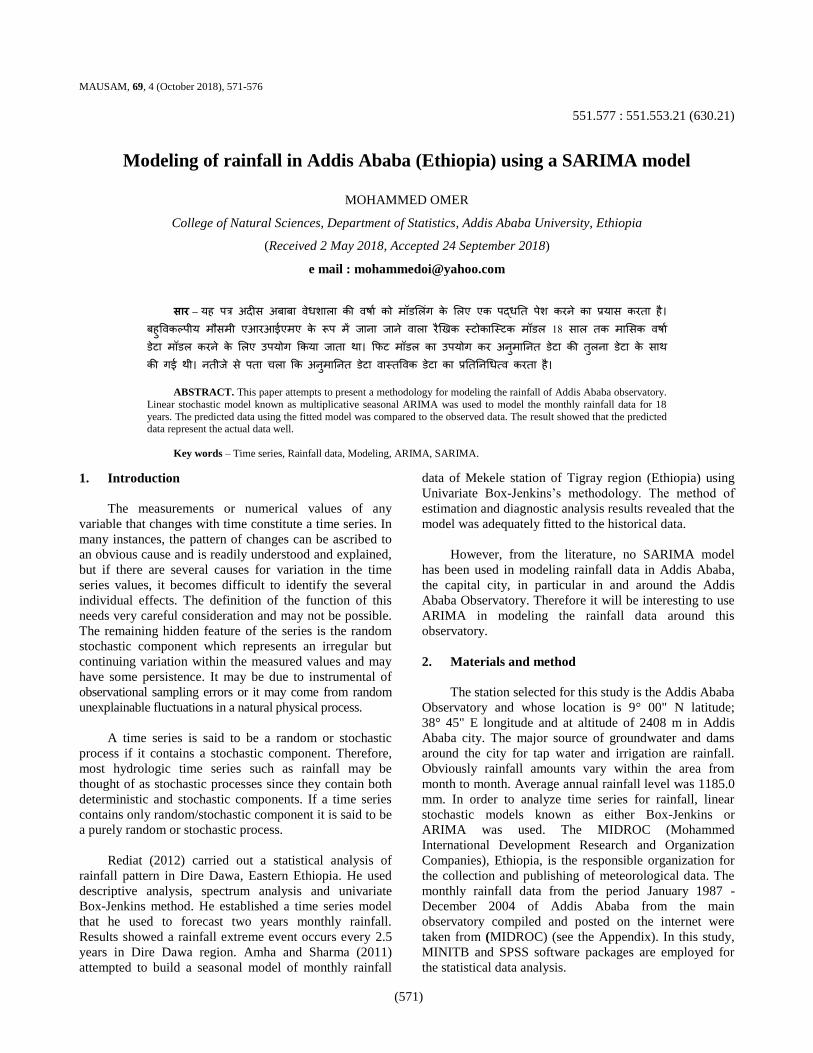
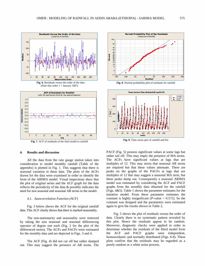
Fig. 6. Residuals versus the order of the data

(Note that order 1 = January 1987)

Fig. 7. ACF of residuals of the final model to rainfall

4. Results and discussion

All the data from the rain gauge station taken into

consideration to model monthly rainfall (Table of the

appendix) is plotted in Fig. 1. This suggests that there is

seasonal variation in these data. The plots of the ACFs

drawn for the data were examined in order to identify the

form of the ARIMA model. Visual inspections show that

the plot of original series and the ACF graph for the data

reflects the periodicity of the data & possibly indicates the

need for non seasonal and seasonal AR terms in the model.

4.1. Autocorrelation Function (ACF)

Fig. 3 below shows the ACF for the original rainfall

data. This ACF clearly shows that there is marked seasonality.

The non-stationarity and seasonality were removed

by taking the non seasonal and seasonal differencing

operator of degree one each (Fig. 2 for the plot of the

differenced series). The ACFs and PACFs were estimated

for the monthly data and are depicted in Figs. 3 and 4.

The ACF (Fig. 4) did not cut off but rather damped

out. This may suggest the presence of AR terms. The

Fig. 8. Normal probability plot of residuals for rainfall

Fig. 9. Time series plot of rainfall and fits

PACF (Fig. 5) possess significant values at some lags but

rather tail off. This may imply the presence of MA terms.

The ACFs have significant values at lags that are

multiples of 12. This may stress that seasonal AR terms

are required but that these values attenuate. There are

peaks on the graphs of the PACFs at lags that are

multiples of 12 that may suggest a seasonal MA term, but

these peaks damp out. Consequently a seasonal ARIMA

model was estimated by considering the ACF and PACF

graphs from the monthly data obtained for the rainfall

(Figs. 4&5). Table 1 shows the parameter estimates for the

tentative model. From these parameter estimates the

constant is highly insignificant (P-value = 0.572). So the

constant was dropped and the parameters were estimated

again to give the results shown in Table 2.

Fig. 5 shows the plot of residuals versus the order of

data. Clearly there is no systematic pattern revealed by

this plot. Hence the residuals appear to be random.

Moreover, diagnostic checks were applied in order to

determine whether the residuals of the fitted model from

the ACF and PACF graphs were independent,

homoscedastic and normally distributed (Figs. 6-8). These

plots confirm that the residuals may be regarded as a

purely random or a white noise process.


Additional to this, the Ljung-Box Q statistics were

estimated for lags 12, 24, 36, and 48 (Table 3). The Q(k)

statistics at these lags were obtained using equation (2)

and are found out to be insignificant (the P-values are

greater than 0.14 for all of them). This shows that the

fitted model is adequate to model the rainfall in and

around the station. Therefore, they emphasize that the

ACFs obtained from the monthly data sequences are not

different from zero. Since the residuals from the model are

normally distributed and homoscedastic, a Box-Cox

transformation of the monthly data was not necessary.

In addition, Fig. 9 shows the relationships between

the observed data for 18-years & the predicted data for the

same years from the model for rainfall. This shows that

the predicted data follow the observed data very closely.

5. Conclusions

Based on the analysis to model rainfall by the seasonal

multiplicative ARIMA model the following conclusions were

drawn: ARIMA model application to the rainfall showed that

predicted data preserved the basic statistical properties of the

observed series. The ARIMA model equation for the rainfall

obtained above may be used for forecasting of rainfall in

A.A. in and around the main observatory.

Acknowledgements

I would like to thank Prof. M. K. Sharma for his

unreserved comments for improvement of the paper and

for suggesting your journal for publication.

The contents and views expressed in this research

paper/ article are the views of the author and do not

necessarily reflect the views of the organizations they

belong to.

References

Akaike, H., 1974, “A Look at the Statistical Model Identification”, IEEE,

Transactions on Automatic Control, AC-19, 716-723.

Amha, G. and Sharma, M. K., 2011, “Modeling and forecasting of

rainfall data of Mekele for Tigray region (Ethiopia)”, Statistics

and Applications, 9, 1&2, (New Series), 31-53.

Box, G. E. P. and Jenkins, G. M., 1976, “Time Series Analysis Forecasting and Control”, Holden-Day, San Francisco.

Chow, V. T., Maidment, D. R. and Mays, L. W., 1988, “Applied Hydrology”, McGraw-Hill Book Company, New York.

Kadri, Y. and Ahmet, K., 2004, “Simulation of Drought Periods Using Stochastic Models”, Turkish J. Eng. Env. Sci., 28, 181-190.

Retrieved on March 31, 2015 from http://journals.tubitak.gov.

tr/engineering/issues/muh-04-28-3/muh-28-3-4-0311-2.pdf.

Ljung, G. M. and Box, G. E. P., 1978, “On a Measure of Lack of Fit in

Time Series Models”, Biometrika, 65, 297-303.

Rediat, T., 2012, “Statistical analysis of rainfall pattern in Dire Dawa,

Eastern Ethiopia using descriptive analysis, cross spectral analysis and univariate Box-Jenkins method”, M. Sc. thesis

submitted to the Department of statistics, University of Addis

Ababa, Ethiopia.

Vandaele, W., 1983, “Applied Time Series and Box-Jenkins Models”,

Academic Press, San Diego.

Wei, W. W. S., 1990, “Time Series Analysis”, Addison-Wesley

Publishing Company Inc. New York.

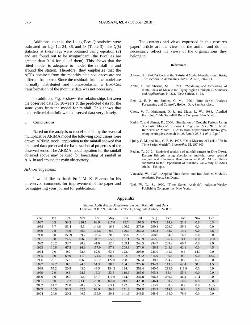
Appendix

Station: Addis Ababa Observatory Element: Rainfall (mm) Data

Location : 9°00" N, Latitude : 38°45" E, Longitude Altitude : 2408 m

Year Jan Feb Mar Apr May Jun Jul Aug Sep Oct Nov Dec

1987 0.5 53.5 236.5 98.9 217.0 99.7 197.5 170.3 114.9 21.8 0.8 0.3

1988 9.7 53.4 5.3 144.6 16.6 106.2 277.9 299.3 229.7 59.9 0.0 0.0

1989 0.8 75.9 76.5 153.6 0.5 120.9 357.2 325.3 188.7 14.5 0.0 7.6

1990 0.8 155.9 59.2 106.4 20.0 88.8 218.7 268.6 184.0 16.2 6.0 0.0

1991 0.0 74.5 106.6 34.7 55.3 191.1 248.9 262.6 126.4 3.4 0.0 50.0

1992 20.2 33.7 20.2 41.0 52.0 109.1 248.5 294.7 209.4 69.7 0.0 2.9

1993 10.8 67.2 16.1 157.9 97.2 208.8 274.0 426.5 243.3 62.1 0.0 4.5

1994 0.0 0.0 82.4 82.6 63.3 123.4 308.9 225.0 141.3 0.5 14.7 0.0

1995 0.0 69.0 41.5 174.4 68.2 102.9 190.2 314.9 136.1 0.0 0.0 48.4

1996 28.1 5.2 106.5 128.2 122.0 258.5 266.4 338.7 294.2 0.2 0.2 0.0

1997 39.2 0.0 24.5 51.3 38.5 104.0 272.6 194.3 113.8 62.4 50.3 1.5

1998 55.2 20.5 43.0 48.5 154.2 124.4 258.4 260.0 213.6 116.9 0.0 0.0

1999 2.9 0.3 28.8 16.3 23.8 119.6 268.6 305.3 88.4 55.4 0.0 0.0

2000 0.0 0.0 2.4 58.7 110.0 144.5 244.8 306.2 250.6 46.4 21.1 0.0

2001 0.0 12.2 213.5 25.0 168.0 213.5 428.0 246.4 130.7 14.6 0.0 0.0

2002 14.7 21.0 90.2 56.5 63.1 172.5 255.2 215.9 108.8 0.2 0.0 16.5

2003 10.5 53.3 62.6 99.9 20.2 151.8 291.8 233.3 214.1 0.8 1.5 54.9

2004 24.8 20.3 49.5 139.9 30.1 141.9 248.5 268.6 164.0 76.9 0.0 0.0

http://journals.tubitak.gov/


Documents

Modeling of rainfall in Addis Ababa (Ethiopia) using a