Embed Size (px)
Citation preview

The Pennsylvania State University
The Graduate School
Department of Engineering Science and Mechanics
MODELING OF PIEZOELECTRIC SMART STRUCTURES FOR
ACTIVE VIBRATION AND NOISE CONTROL APPLICATIONS
A Thesis in
Engineering Science and Mechanics
by
Senthil V Gopinathan
2001 Senthil Gopinathan
Submitted in Partial Fulfillment of the Requirements
for the Degree of
Doctor of Philosophy
August 2001

We approve the thesis of Senthil V Gopinathan.
Date of Signature
Vasundara V Varadan Distinguished Professor of Engineering Science and Mechanics Thesis advisor Co-Chair of Committee
Vijay K Varadan Distinguished Alumni Professor of Engineering Science and Mechanics and Electrical Engineering Co-Chair of Committee
Sabih I Hayek University Distinguished Professor of Engineering Mechanics
Eduard S. Ventsel Professor of Engineering Science and Mechanics
Stephen A. Hambric Assistant Professor of Acoustics
R. P. McNitt Professor of Engineering Science and Mechanics Head of the Department of Engineering Science and Mechanics

iii
ABSTRACT
Active vibration control and active structural acoustic control using piezoelectric
sensors and actuators have recently emerged as a practical and promising technology.
Efficient and accurate modeling of these structures bonded to or embedded with actuators
and sensors is needed for efficient design of smart structures. This dissertation addresses
the modeling of these structures and the associated control system design technique.
Modeling of structures with both laminated and discrete type of actuators and sensors are
addressed.
For piezoelectric laminates the governing equations of motion are derived using
First Order Shear Deformation Theory (FSDT) and for the first time the dynamic
response fields inside the laminate are obtained and compared with full elasticity
solutions. This comparison brought out the effect of assumptions made with respect to the
electric and mechanical fields using FSDT and Classical Laminate Theory (CLT) in
previous work. It is expected that this analysis and the interior field estimations would
help designers to understand the shortcomings of FSDT in modeling piezoelectric
laminates, and help them to adopt this theory properly for use in FE or other numerical
models.
For surface bonded discrete patch type actuators/sensors, the governing dynamic
equation of motion for a plate is derived. The solution to this equation is obtained using a
Fourier series method and the effect of passive stiffness and mass on the natural
frequency is studied. The studies showed that ignoring the mass and the passive stiffness

iv
of actuators/sensors leads to large errors in estimating the vibration characteristics of the
smart plate. A Rayleigh-Ritz (RR) approach is then presented for studying the active
vibration and transmitted noise control of a smart plate with discrete piezoelectric
patches. Classical laminated plate theory is used to model the composite plate and electro
elastic theory is used model the piezoelectric patches. The dynamic equations of motion
for the coupled smart panel-cavity system are derived using Hamilton’s principle. Close
agreement between the present approach and the finite element and experimental results
confirmed the validity of the approach. The RR approach is thus presented as a simple,
computationally inexpensive approach when compared to the finite element method. The
RR method also proved to be powerful method for modeling the adjacent acoustic
medium and for the associated control system design.
A finite element approach for the integrated design of a structure and its control
system for suppressing vibration and the radiated noise are presented. A finite element
model for a smart plate with surface bonded piezoelectric patches is developed using
shell, brick and transition elements. The free and forced vibration characteristics of the
plate are studied with and without closed loop feedback control. An optimal (multi-input
multi-output) MIMO controller design for the vibration suppression of a clamped plate
using the FE model is proposed. Numerical simulation showed that an optimal controller
designed for controlling the smart plate vibration also reduces the transmitted noise to 20
dB for the first mode and to 40 dB for the second mode of plate.
The RR approach accurately models rigid walled acoustic cavities, but flexible

v
elastic boundaries or sound absorbing walls cannot be modeled using this approach. To
model such acoustic domains, a novel hybrid Rayleigh-Ritz/Boundary Element solution
method is proposed. This method would enable designers to model the panel with
piezoelectric actuators and sensors and the adjacent acoustic medium with the presence of
passive absorbers at the interface. The predicted sound pressure attenuation for three
different thicknesses of passive absorber in the frequency range of 200 to 1200 Hz is
calculated and an optimal thickness value of for the absorber for the smart panel is
calculated. The attenuation in sound pressure levels due to an active control system in
the presence of passive absorber is also computed. The system matrices resulting from
this method are very smaller in size when compared to the FE models, which makes this
approach most suitable for optimization studies. This new approach can be further
extended to model the more complicated acoustic enclosures with complex interface
conditions.

vi
Table Of Contents
LIST OF FIGURES .......................................................................................................... x
LIST OF TABLES ......................................................................................................... xiv
ACKNOWLEDGEMENT .............................................................................................. xv
CHAPTER 1 INTRODUCTION ..................................................................................... 1
1.1 BACKGROUND...................................................................................................... 1
1.2 ACTIVE STRUCTURAL ACOUSTIC CONTROL ......................................................... 3
1.3 ACTUATION AND SENSING MATERIALS ............................................................... 6
1.4 SMART STRUCTURE MODELING ISSUES................................................................ 9
1.5 OBJECTIVES OF THE PRESENT RESEARCH .......................................................... 10
1.6 SCOPE OF THESIS ............................................................................................... 12
CHAPTER 2 RESEARCH BACKGROUND............................................................... 14
2.1 INTRODUCTION................................................................................................... 14
2.2 MODELS FOR PIEZOELECTRIC LAMINATES ......................................................... 14
2.3 MODELS FOR SMART STRUCTURES WITH DISCRETE PIEZOELECTRIC PATCHES .. 18
2.4 MODELS FOR VIBROACOUSTIC SYSTEMS WITH SMART STRUCTURES................. 20
2.5 CLOSURE............................................................................................................ 22
CHAPTER 3 FIRST ORDER SHEAR DEFORMATION THEORY FOR
PIEZOELECTRIC LAMINATES ................................................................................ 23
3.1 INTRODUCTION................................................................................................... 23
3.2 FIRST ORDER SHEAR DEFORMATION LAMINATE THEORY .................................. 23

vii
3.2.1 Sensor Problem ......................................................................................... 26
3.2.2 Actuator Problem ...................................................................................... 31
3.3 METHOD OF SOLUTION ...................................................................................... 34
3.3.1 Sensor Solution.......................................................................................... 35
3.3.2 Actuator Solution....................................................................................... 36
3.4 ELASTICITY SOLUTION....................................................................................... 38
3.5 RESULTS AND DISCUSSION ................................................................................ 44
3.6 SUMMARY .......................................................................................................... 50
CHAPTER 4 MODELING OF VIBRATION AND NOISE CONTROL USING
DISCRETE PIEZOELECTRIC ACTUATORS/SENSORS
-A) FOURIER SERIES METHOD B) RAYLEIGH-RITZ APPROACH 80
4.1 INTRODUCTION................................................................................................... 80
4.2 PIEZOELECTRIC PATCHES: MODELING AND FORMULATION............................... 83
4.2.1 Actuator Patch Model ............................................................................... 86
4.2.2 Sensor Patch Model .................................................................................. 87
4.3 SMART PLATE MODEL........................................................................................ 88
4.4 SOLUTION METHOD ........................................................................................... 91
4.5 RESULTS AND DISCUSSION ................................................................................ 93
4.6 ACTIVE ENCLOSURE NOISE CONTROL USING RAYLEIGH-RITZ METHOD............ 96
4.7 POTENTIAL AND KINETIC ENERGIES OF THE SYSTEM ....................................... 97
4.7.1 Composite Plate ........................................................................................ 97

viii
4.7.2 Piezoelectric Patches ................................................................................ 98
4.7.3 Acoustic Cavity.......................................................................................... 99
4.8 DYNAMIC EQUATION OF MOTION: SMART PANEL-CAVITY SYSTEM.................. 99
4.9 RESULTS AND DISCUSSION .............................................................................. 102
4.10 SUMMARY ........................................................................................................ 110
CHAPTER 5 FINITE ELEMENT SIMULATION OF SMART PANELS FOR
VIBRATION AND NOISE CONTROL APPLICATIONS ...................................... 112
5.1 INTRODUCTION................................................................................................. 112
5.2 FORMULATION ................................................................................................. 116
5.2.1 Finite Element Model Of The Panel Structure........................................ 116
5.2.2 Condensation of System Matrices ........................................................... 120
5.3 CONTROL MECHANISM .................................................................................... 121
5.3.1 Direct Charge Approach......................................................................... 122
5.3.2 Direct Voltage Approach ........................................................................ 123
5.4 EIGENVALUE ANALYSIS ................................................................................... 124
5.4.1 Modal Analysis........................................................................................ 125
5.5 OUTPUT FEEDBACK OPTIMAL CONTROL .......................................................... 126
5.6 RADIATED SOUND FIELD INSIDE A RECTANGULAR ENCLOSURE ...................... 129
5.7 NUMERICAL SIMULATIONS OF THE CLAMPED PLATE ....................................... 131
5.8 SUMMARY ........................................................................................................ 141
CHAPTER 6 DEVELOPMENT OF A RAYLEIGH-RITZ/BOUNDARY
ELEMENT MODELING APPROACH FOR ACTIVE/PASSIVE CONTROL .... 143

ix
6.1 INTRODUCTION................................................................................................. 143
6.2 BOUNDARY ELEMENT MODEL FOR ACOUSTIC ENCLOSURE............................. 145
6.2.1 Dual Reciprocity Method ........................................................................ 145
6.3 FLUID-STRUCTURE COUPLING ......................................................................... 149
6.4 PLATE-CAVITY INTERFACE .............................................................................. 151
6.5 RESULTS AND DISCUSSION............................................................................... 153
6.6 SUMMARY ........................................................................................................ 158
CHAPTER 7 CONCLUSIONS AND FUTURE WORK........................................... 159
7.1 INTRODUCTION................................................................................................. 159
7.2 CONCLUSIONS AND FUTURE WORK ................................................................. 159
REFERENCES.............................................................................................................. 163
APPENDIX A CONSTITUTIVE RELATIONS FOR A PIEZOELECTRIC
MEDIUM ....................................................................................................................... 176
APPENDIX B BE FORMULATION FOR THE ACOUSTIC DOMAIN .............. 178

x
List Of Figures
Figure 1.1The sound pressure level spectrum inside the helicopter cabin.......................... 2
Figure 1.2 Piezoelectric laminate with Feedback circuit .................................................... 7
Figure 3.1 Undeformed and deformed configuration of the piezoelectric laminate ......... 24
Figure 3.2 Configuration of the piezoelectric laminate..................................................... 27
Figure 3.3 Axial Displacement (v) for Sensor Case (l/h = 20) ......................................... 53
Figure 3.4 Transverse Displacement (w) for Sensor Case (l/h = 20)................................ 53
Figure 3.5 Electric Potential (φ) for Sensor case (l/h = 20) ............................................. 54
Figure 3.6 Bending Stress (σy) for Sensor case (l/h = 20) ................................................ 54
Figure 3.7 Transverse Normal Stress for Sensor Case (l/h = 20)...................................... 55
Figure 3.8 Shear Stress for Sensor case (l/h = 20) ............................................................ 55
Figure 3.9 Bending strain for Sensor case (l/h = 20) ........................................................ 56
Figure 3.10 Transverse normal strain for Sensor case (l/h = 20) ..................................... 56
Figure 3.11 Shear strain for Sensor case (l/h = 20)........................................................... 57
Figure 3.12 y Component of the Electric Field for Sensor Case (l/h = 20)...................... 57
Figure 3.13 z Component Electric Field for Sensor Case (l/h = 20) ................................. 58
Figure 3.14 y component Electric Displacement for Sensor Case (l/h = 20) .................... 58
Figure 3.15 z component Electric Displacement for Sensor Case (l/h =20) ..................... 59
Figure 3.16 Axial Displacement for Actuator case (l/h = 20)........................................... 60
Figure 3.17 Transverse Displacement for Actuator Case (l/h = 20) ................................. 60
Figure 3.18 Electric Potential Actuator case (l/h = 20)..................................................... 61
Figure 3.19 Bending Stress for Actuator case (l/h = 20)................................................... 61
Figure 3.20 Transverse Normal Stress Actuator Case (l/h = 20) ...................................... 62
Figure 3.21 Shear Stress for Actuator case (l/h = 20) ....................................................... 62
Figure 3.22 Bending strain for Actuator case (l/h = 20) ................................................... 63
Figure 3.23 Transverse normal strain for Actuator case (l/h = 20) ................................... 63
Figure 3.24 Shear strain for Actuator case (l/h = 20)........................................................ 64

xi
Figure 3.25 y Component Electric Field for Actuator case (l/h = 20)............................... 64
Figure 3.26 z Component Electric Field for Actuator case (l/h = 20)............................... 65
Figure 3.27 y component of the Electric Displacement for Actuator case (l/h = 20)........ 65
Figure 3.28 z Component Electric Displacement for Actuator case (l/h = 20) ................. 66
Figure 3.29 Axial Displacement for Sensor case (l/h = 50) .............................................. 66
Figure 3.30 Transverse Displacement for Sensor Case (l/h = 50) .................................... 67
Figure 3.31 Electric Potential for Sensor case (l/h = 50) ................................................. 68
Figure 3.32 Bending Stress for Sensor case (l/h = 50)...................................................... 68
Figure 3.33 Bending strain for Sensor case (l/h = 50) ...................................................... 69
Figure 3.34 Shear Stress for Sensor case (l/h = 50) .......................................................... 69
Figure 3.35 Transverse Normal Stress for Sensor Case (l/h = 50).................................... 70
Figure 3.36 Transverse normal strain for Sensor case (l/h = 50) ...................................... 70
Figure 3.37 Shear strain for Sensor case (l/h = 50)........................................................... 71
Figure 3.38 y Component Electric Field for Sensor case (l/h = 50).................................. 71
Figure 3.39 z Component Electric Field for Sensor case (l/h = 50) .................................. 72
Figure 3.40 y component Electric Displacement for Sensor case (l/h = 50)..................... 72
Figure 3.41 z Component Electric Displacement for Sensor case (l/h = 50) .................... 73
Figure 3.42 Axial Displacement for Actuator case (l/h = 50)........................................... 73
Figure 3.43 Transverse Displacement for Actuator Case (l/h = 50) ................................. 74
Figure 3.44 Electric Potential for Actuator case (l/h = 20) ............................................... 74
Figure 3.45 Bending Stress for Actuator case (l/h = 50)................................................... 75
Figure 3.46 Transverse Normal Stress for Actuator Case (l/h = 50)................................. 75
Figure 3.47 Shear Stress for Actuator case (l/h = 50) ....................................................... 76
Figure 3.48 Bending strain for Actuator case (l/h = 50) ................................................... 76
Figure 3.49 Transverse normal strain for Actuator case (l/h = 50) ................................... 77
Figure 3.50 Shear strain for Actuator case (l/h = 50)........................................................ 77
Figure 3.51 y Component Electric Field for Actuator case (l/h = 50)............................... 78
Figure 3.52 z Component Electric Field for Actuator case (l/h = 50)............................... 78
Figure 3.53 y component Electric Displacement for Actuator case (l/h = 50).................. 79

xii
Figure 3.54 z Component Electric Displacement for Actuator case (l/h = 50) ................. 79
Figure 4.1 Configuration of the surface bonded piezoelectric patch ............................... 83
Figure 4.2 Convergence of the frequencies....................................................................... 94
Figure 4.3 Variation of the resonant frequencies with patch size for
PVDF/Plexiglas/PVDF.................................................................................... 95
Figure 4.4 Variation of the resonant frequencies with patch size for PZT/Al/PZT.......... 95
Figure 4.5 Cavity with smart panel and acoustic excitation ........................................... 104
Figure 4.6 Amplification function for mode 1 ................................................................ 107
Figure 4.7 Amplification function for mode 2 ................................................................ 107
Figure 4.8 Amplification function for mode 3 ................................................................ 108
Figure 4.9 Amplification function for mode 4 ................................................................ 108
Figure 4.10 Experimental Setup For Noise Control Measurement................................. 109
Figure 4.11 The pressure and the amplitude measured by the accelerometer and the
Microphone ................................................................................................. 109
Figure 5.1 An elastic continuum with piezoelectric elements and external forces ......... 118
Figure 5.2 Aluminum panel with five surface bonded collocated piezoelectric
actuators/sensors and Schematic diagram of two loading cases ................... 132
Figure 5.3 Modeling of a geometrical transition with several types of finite
element. .......................................................................................................... 132
Figure 5.4 Finite element model with piezoelectric sensors and actuators..................... 133
Figure 5.5 Mode shapes of the clamped plate containing piezoelectric patches............. 134
Figure 5.6 Root locus plot of the optimal closed loop system for various ri .................. 135
Figure 5.7 Frequency spectrum at point A when harmonic excitation is applied at
point A. (with optimal feedback gain for case I)............................................ 136
Figure 5.8 Time history plot at point A when a unit step excitation is applied at
point A............................................................................................................ 136
Figure 5.9 Response of the clamped plate at point F due to three arbitrary
harmonic forces (No control) ........................................................................ 137

xiii
Figure 5.10 Time history plot of the effect of the optimal gain at point F...................... 138
Figure 5.11 Acoustic field in (vertical plane of the cavity) enclosure when first
mode of panel is excited............................................................................... 140
Figure 5.12 Acoustic field in vertical plane of the cavity enclosure when fourth
mode is excited............................................................................................. 140
Figure 6.1 Acoustic cavity with smart panel and absorber ............................................. 149
Figure 6.2 Structural and fluid velocities at fluid-structure interface ............................. 150
Figure 6.3 Boundary element mesh for the cavity .......................................................... 153
Figure 6.4 Excitation flux on the top surface of the cavity ............................................. 154
Figure 6.5 Time History of the flux at midpoint of the bottom face............................... 155
Figure 6.6 Real part value curves of the admittance for the different thickness
Of foamed aluminum .................................................................................... 156
Figure 6.7 Predicted sound pressure attenuation for different thickness of foam........... 157
xiv
List Of Tables
Table 1.1 Comparison of solid-state actuation materials provide significant
Actuation ............................................................................................................ 8
Table 3.1 Material Properties For the three-layer laminate beam..................................... 45
Table 3.2 Natural Frequencies for single and three layered laminate beams.................... 46
Table 4.1 Material Properties for the plate and piezoelectric patches .............................. 93
Table 4.2 Natural frequencies of the smart plate .............................................................. 94
Table 4.3 Material and geometric properties of smart panel-Cavity system .................. 103
Table 4.4 Uncoupled resonant frequencies (RR method) and comparison with FE
Solution ........................................................................................................... 104
Table 4.5 Coupled frequencies of the smart panel-cavity............................................... 105
Table 4.6 Transmitted noise inside the cavity (RR method)........................................... 105
Table 6.1 The resonant frequencies of the cavity............................................................ 153
Table 6.2 Coupled resonant frequencies of the cavity .................................................... 157

xv
ACKNOWLEDGMENTS
I would like to express my sincere gratitude to my advisor, Professor Vasundara
V. Varadan for giving me the opportunity to work with her, and for her valuable and
insightful guidance throughout this work. Her support and encouragement, in academic
as well as non-academic matters, during my graduate studies at Penn State made the
whole experience highly supportive and educational. Also, I wish to express my sincere
thanks to my co advisor, Professor Vijay K. Varadan for his valuable inputs, and critical
suggestions at various points of this work, which made this thesis stronger. Also the
financial support from the Center for the Engineering of Electronic and Acoustic
materials and devices is gratefully acknowledged.
I am grateful to members of my doctoral committee, Dr. Sabih I Hayek, Dr.
Eduard Ventsel and Dr. Stephen Hambric for their careful review and advice during the
course of research.
Special thanks to all the members of the research center, for their continuous
encouragement and support. Especially, I would like to thank Dr. Jose, Dr. Sharma, Dr.
Lim and all my fellow graduate students. My thanks to all my friends Sunil, Iyer, Kartik,
Vinoy, Anil, Nikhil, CV and Sanjay who made my stay very pleasant at State College.
I am indebted to my parents and my parents in law for supporting and
encouraging me throughout my graduate studies. This work would not have been possible
without their motivation and support.

xvi
This work and its associated accomplishments would not have been possible
without the affection and sacrifice of my family; Vanathi, Navaneeth and Shakthi Sharan.
This study is dedicated to them.

1
Chapter 1 INTRODUCTION
1.1 Background
During the last two decades there has been an accelerating level of interest in the
control of sound by active techniques. Many of the physical principles involved have
long been established, but the technological means for the successful implementation of
active noise control have only recently become feasible. Noise radiation and sound
transmission from vibrating structures e.g., automobile bodies, aircraft fuselages and
cabins, industrial machinery, etc., are common problems in noise control practices. Two
such areas of application are the control of propeller noise in the passenger cabins of
aircraft, and the control of low frequency engine-induced noise inside cars.
High acoustic levels are present within these enclosures (Von Flotow and
Mercadel, 1995), typically caused by propellers or engine fan spool speed imbalances
transmitted via the wing structure, or periodic pressures exerted on the cabin from
passing propeller blades. Early noise control strategies for aircraft cabins were based on
field cancellation techniques, employing microphone sensors, and speakers as acoustic
actuators. These techniques are most effective at low frequencies and easier to implement
for periodic sound fields than for random sound fields. For example the sound pressure
level inside the passenger cabin of helicopters shows (Figure 1.1) (Wilby 1996) strong
components at 15 to 20 Hz, which correspond to the Blade Passing Frequency (BPF) of

2
the main rotor. Although this noise component is below the lower frequency limit of
hearing, prolonged exposure will decrease the comfort of the passengers.
The primary contributions to the noise spectrum in a helicopter are the main rotor,
tail rotor and turbines, which operate at frequencies ranging from 50 to 500 Hz and the
gear mechanisms in the main transmission, which operate at frequencies above 500 Hz.
Likewise, the sound pressure spectrum inside the passenger compartments of a propeller
aircraft contains strong tonal components at harmonics of the BPF of the propellers,
which are difficult to attenuate the using passive absorption (Metzger, 1981; Wilby et al.,
1980). The noise cancellation technique typically demonstrated 10 to 15 dB reductions in
Figure 1.1 The sound pressure level spectrum inside the helicopter cabin (G. Niesl, E. Laudien)

3
sound pressure levels over the first several harmonics of the propeller blade passage
frequency. However, reductions were highly spatial, and required many sources (up to
32) for achieving control for small turboprop aircraft (Elliott, 1989). These numbers are
required due to the spatial mismatch between the primary acoustic field and the field
produced by the interior sources (speakers), creating an interior acoustic field that is more
broadband in nature. More details can be obtained on the practical active control system
operating in the passenger cabin from references Elliott et al (1989a) and Silcox (1990).
Apart from having to track the excitation frequency, the noise control task inside
the car cabin is less extensive than in the aircraft case since the volume of the enclosure is
smaller, and fewer loudspeakers and microphones need to be used. At the lowest
frequency, only a single loudspeaker and microphone would be needed, which could
control a single dominant acoustic mode (Oswald 1984).
1.2 Active Structural Acoustic Control
A more direct approach for noise control makes use of the fact that the acoustic
field must pass through the structure. The control of radiated noise is achieved via
controlling the vibration of flexible walls and other radiating structures. The methods for
suppressing the vibration and the radiated noise from structural members or mechanical
components are identified as “Structural Acoustic Control” (SAC), and are classified into
two major categories, namely passive and active control methods. The underlying
technique in these methods is to alter the vibration characteristics of the radiating
structural members and thereby minimize the radiated sound field. Some examples of
these radiating structural members are airplane fuselage panels, helicopter cabin panels,

4
and compressor housings. The first method involves altering the vibration characteristics
of structures passively by tailoring their material properties. The second strategy involves
altering the vibration characteristics by placing actuators at pre-selected points on the
structures and driving these actuators to a predetermined force amplitude and phase.
Traditional means for the control of undesired sound and vibration are often referred to as
passive methods since no power source is required for the control system. The noise
reduction is achieved by either insulating the enclosure walls or by covering them with
porous sound absorbers. These passive control methods are quite effective at high
frequencies or in narrow frequency bands. The thickness requirement for a passive
absorber at lower frequencies is impractical. For example, at low frequency near 200 Hz,
the wavelength of the sound is approximately 1.7 meters and efficiently designed passive
absorbers for the enclosure wall would be more than a meter in thickness to absorb the
sound energy. So the active control method is an attractive alternative to passive methods
at these low frequencies.
The active control of vibration and structurally radiated noise also known as
Active Structural Acoustic Control (ASAC) using active materials has emerged as a
viable technology in recent years. The past decade has seen great advances towards
integrating actuators and sensors with electro-active materials into devices and structures.
The new design paradigms focus on constructing smaller, more precise systems with
emphasis on improving performance and efficiency while meeting increasingly stringent
weight, size, and power requirements. This has led to the development of various systems
using piezoelectrics, electrostrictors, and shape memory ceramics, and other active

5
materials (Crawley 1987). A material, which can sense and respond to one or more
external stimuli such as pressure, temperature, voltage, electric and magnetic fields,
chemicals etc., can be called as an active material. Active materials (also sometimes
called smart materials) and structures integrated with these materials have gained
worldwide attention in the past few years because of their application in every branch of
engineering. Actuators and sensors are becoming integral parts of the structures, which
are making the host structures more ‘adaptive’ or ‘smart’. These piezoelectric transducers
are used to control beam (Varadan V.K et al, 1990), truss (V. V. Varadan et al, 1993),
plates (V.V. Varadan et al, 1991) and shell structures (Tzou et al 1993b). Varadan V. V.
et al (1991) showed that the active control of vibration and radiated noise using
piezoelectric sensors and actuators is a practical and feasible approach for plate
structures. In this work authors have observed that when using an analog controller, the
experimentally measured radiated noise showed a maximum reduction of 20 dB. In
another experimental investigation of active control of transmitted sound through a plate
into a cubic sound enclosure, Xiaoqi Bao et al (1995) showed that one actuator/sensor
control system successfully reduced the sound level at the first three resonance
frequencies by 15-22 dB. Vibration suppression of the fuselage structure has been studied
using both point force devices (shakers) and in-plane bonded piezoceramics as actuators
(Silcox et al., 1993; Fuller et al., 1992), illustrating reductions in interior noise levels
similar to those obtained with speaker sources. More importantly, these reductions can be
broadband in nature, are global throughout the structure, and can be achieved with far
few actuator sources. Several full-scale demonstrations have also shown that
6
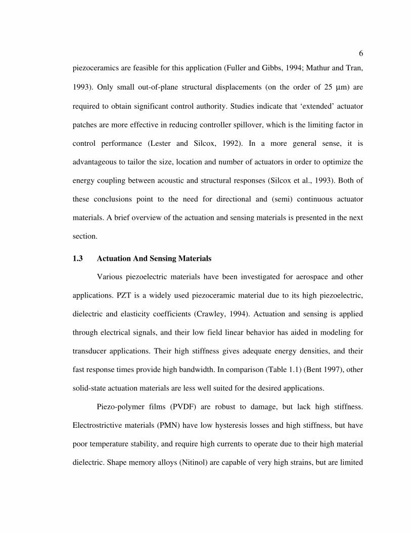
piezoceramics are feasible for this application (Fuller and Gibbs, 1994; Mathur and Tran,
1993). Only small out-of-plane structural displacements (on the order of 25 µm) are
required to obtain significant control authority. Studies indicate that ‘extended’ actuator
patches are more effective in reducing controller spillover, which is the limiting factor in
control performance (Lester and Silcox, 1992). In a more general sense, it is
advantageous to tailor the size, location and number of actuators in order to optimize the
energy coupling between acoustic and structural responses (Silcox et al., 1993). Both of
these conclusions point to the need for directional and (semi) continuous actuator
materials. A brief overview of the actuation and sensing materials is presented in the next
section.
1.3 Actuation And Sensing Materials
Various piezoelectric materials have been investigated for aerospace and other
applications. PZT is a widely used piezoceramic material due to its high piezoelectric,
dielectric and elasticity coefficients (Crawley, 1994). Actuation and sensing is applied
through electrical signals, and their low field linear behavior has aided in modeling for
transducer applications. Their high stiffness gives adequate energy densities, and their
fast response times provide high bandwidth. In comparison (Table 1.1) (Bent 1997), other
solid-state actuation materials are less well suited for the desired applications.
Piezo-polymer films (PVDF) are robust to damage, but lack high stiffness.
Electrostrictive materials (PMN) have low hysteresis losses and high stiffness, but have
poor temperature stability, and require high currents to operate due to their high material
dielectric. Shape memory alloys (Nitinol) are capable of very high strains, but are limited

7
to ultra-low bandwidth applications (< 5 Hz) due to the time needed for thermal
dissipation/heating. Finally, magnetostrictive actuators (Terfenol-D) have similar
actuation energy density and bandwidth as piezoceramics, but are very heavy when the
coils and flux path materials are accounted for. The actuators and sensors are
incorporated into the host structures in many different forms depending upon the
environmental and operating requirements of the host structure. Beams, truss structures,
plate and shell-like structures are frequently used host structures for piezoelectric sensors
and actuators for vibration and noise control applications. Several have been conceived
experimentally such as for vibration control (for plates Bayer et al, 1991, Ghidella and
Steven 1994; for beams—Bailey and Hubbard 1985), shape control (Koconis et al 1994),
and buckling control (Thompson and Loughlan 1995). The actuators and sensors could
either be surface bonded or embedded inside the layers in the form of lamina or fibers
(Bent 1997) of the host laminate. A piezoelectric laminate with feedback control circuit is
shown in Figure 1.1.
Figure 1.2 Piezoelectric laminate with Feedback circuit
1 , 3 Piezoelectric layer 2 Non-piezoelectric layer
G 1
2
3

8
Because of its very stiff and brittle nature, the fabrication of laminates containing
PZT layers will be a challenge. Also PZT cannot be subjected to very high temperatures
when fabricating the laminates, to prevent depoling and loss of piezoelectric properties.
Again, for the surface bonded actuators and sensors the size and shape of these
actuators/sensors vary depending on the application for which it is designed
Table 1.1 Comparison of solid-state actuation materials that provide significant actuation
Rectangular or circular patches are the most common form for actuators and
sensors in noise and vibration control applications. Development of simple and accurate
models, analysis methods, and a reliable controller design for the structures bonded with
the piezoelectric layers or patches are interesting areas of research.
This dissertation deals with modeling of both patch type and film type
actuators/sensors for vibration and noise control purposes. There are numerous other
aerospace and related field applications that can or do utilize active materials to achieve
improved performance: structural health monitoring, damage mitigation, and de-icing, to
name a few. The models and analysis approaches developed in the present work can be
PZT5H PVDF PMN Terfenol D Nitinol Actuation
Mechanism Piezoceramic Piezofilm
Electro-strictive
Magneto-strictive
Shape memory
Max strain 0.13% 0.07% 0.1% 0.2% 2% -8%
Modulus (GPA) 60.6 2 64.5 29.7 75(hi-tem)- 28(lo-temp)
Density (Kg/m3) 7500 1780 7800 9250 7100
Temp Range -20 to 200oC Low 0 to
40oC High -
Useful frequency range
0-100 MHz 0-10 MHz 100 kHz <10 kHz <5 Hz
Actuation Energy density
(J/Kg) 6.83 0.28 4.13 6.42 252-4032

9
used or extended without any difficulty for these applications.
1.4 Smart Structure Modeling Issues
In order to achieve low weight, smaller size and cost-effective design of smart
structures using strain sensing and actuation properties of piezoelectric materials, we
need accurate and reliable models for analysis and design. To develop such models, the
interaction between the structure and the actuators/sensors must be well understood.
There have been many theories and models proposed for analysis of laminated composite
beams and plates containing active and passive piezoelectric layers. Early research in the
design and analysis of smart structures for various applications used simplified theories
and models for various types of structures. Classical (closed form solutions), numerical
(such as finite difference), and physical modeling (such as finite element and boundary
element) approaches have been extensively used to predict and analyze characteristics of
the structures and machinery. However, the continuous demand for more precise systems
has forced researchers and engineers to search for more accurate and efficient models to
investigate the dynamics of structures with attached (or embedded) smart devices.
Some of the earliest models (Crawley and de Luis 1987, Bailey and Hubbard
1985, Robbins and Reddy 1991) used the induced strain by the piezoelectric actuators as
an applied strain that contributed to the total strain of the non-active structure, similar to a
thermal strain contribution. However, for complex intelligent structures with a significant
amount of sensors and actuators distributed in the structure, the electro-mechanical
coupling within the piezoelectric material as well as the coupling with the substrate must

10
be more fully integrated into the formulation. To find analytical solutions, electrical and
mechanical equilibrium or governing field equations have to be solved for a set of
boundary conditions (e.g. for plates—Heyliger 1997). The coupling of the electrical and
mechanical constitutive equations will lead to the coupling of some boundary conditions.
Hence, applying mechanical boundary conditions in the conventional way may not
always be correct due to the coupling with electrical boundary conditions. In addition,
analytical solutions often assume the solution with a certain series form and establish
coefficients using the governing equations of mechanics. Since the assumed solution
depends on the geometry of the structure, a set of solutions derived for rectangular plates
would not be applicable to a circular plate structure or any other type of geometry. An
alternative to solving exact analytical equations is to use finite element analysis (FEA). A
truly sophisticated smart or intelligent structure is a composite of active and non-active
materials and thus all coupling between actuators, substrate and sensors must be included
in the model. This requirement is effectively facilitated by the Hamilton variational
principle or energy methods. The variational principle based FE formulation is an
effective method for complex structures because mechanical and electrical equilibrium
equations do not need to be solved explicitly. The physics of the entire structure has been
fully accounted for in the energy integrals and there is no need to derive equations based
on forces and moments
1.5 Objectives Of the Present Research
As we have seen from the overview of the previous research carried out in this

11
area the modeling approach and analysis techniques differ considerably between the
laminated type smart structures and smart structures bonded with the discrete type active
materials. The objective of this thesis is to present a linear modeling approach and
analysis method for analyzing smart structures. There are five major components to the
work being presented here.
1. First order Shear deformation model for piezoelectric laminates.
2. Classical laminated plate model for smart plates incorporating patch type
actuators/sensors.
3. Finite element modeling and demonstration of closed loop feedback
control for vibration and radiated noise control application.
4. Demonstration of Rayleigh-Ritz analysis method using the model
developed for smart structures.
5. A novel and efficient method of coupling the Rayleigh-Ritz approach for
the smart panel with the Boundary Element formulation for the cavity.
The first two models would contribute to the smart structure design and analysis
community to use more accurate models for analysis and better understanding of the
behavior of these electromechanical materials when used as an actuators or sensors in
aerospace structures. The third and fourth models are aimed at the development of closed
loop active radiated noise control analysis techniques using the finite element and
Rayleigh Ritz approaches. These methods are applied for the first time for noise control
applications using closed loop feedback techniques.

12
1.6 Scope Of Thesis
The objective of the present thesis work is to develop the linear modeling
techniques for electromechanically coupled material to the extent which would permit
analysis of structures incorporating active materials.
The review of the previous research related to this dissertation is presented in
chapter 2. The various models and analysis methods developed for the analysis of smart
structures for various applications are reviewed and their merits and drawbacks are
discussed.
The development of the First Order Shear Deformation Theory (FSDT) for
piezoelectric laminates is presented in Chapter 3. The electric and mechanical fields
obtained using this FSDT model is compared with fields obtained using full electroelastic
models for the laminate.
This is followed by the development of an electroelastic model for plates with
surface bonded discrete piezoelectric patches presented in chapter 4. Two methods of
solution approaches are attempted. Firstly, a Fourier series method is presented to solve
the dynamic equations resulting from this model. Secondly, using the analytical model
developed for the smart structure a vibroacoustic system with a smart panel is studied
using the Rayleigh-Ritz approach and active control of noise transmitted into a
rectangular enclosure is demonstrated.
Chapter 5 is dedicated to the formulation of the linear finite element model for the
closed loop vibration and radiated noise. The smart structure is modeled using the flat
shell and brick elements and the acoustic cavity is modeled using the rigid walled cavity

13
modes.
Chapter 6 presents an elegant approach for the active noise control problems by
coupling the Rayleigh-Ritz model of the host structure and the dual reciprocity boundary
element model of the acoustic cavity.
Chapter 7 closes the thesis with a summary of the contributions and
recommendations for future work in the modeling of smart structures for active vibration
and radiated noise control applications.
.

14
Chapter 2
RESEARCH BACKGROUND
2.1 Introduction
The references listed in this chapter are grouped under three major categories.
Group I consists of references that are related to the previous models developed for
analysis of piezoelectric laminates. Previous works on both analytical and finite element
models are presented in this section. Group II references are related to the models
developed for the smart structure attached with patch type actuators/sensor. In group III,
previous research carried out on developing vibroacoustic models, which include smart
materials and on the control system design for smart structures are discussed.
2.2 Models for Piezoelectric Laminates
The development of smart composites offers great potential for advanced
aerospace structural applications. Piezopolymeric and piezoceramic are employed as both
actuators and sensors in the development of these structures by taking advantage of direct
and converse piezoelectric effects. The modeling of piezoelectric laminates can be
enhanced in two ways; more accurate mechanics models to address the characteristics of
composite laminates and more accurate electroelastic models which addresses the
coupling effects between the electrical and mechanical fields inside the actuators and
sensors.

15
The fundamental work of Tiersten (1969) gave much of the necessary theoretical
development for the static and dynamic behavior of a single-layer piezoelectric plate. Lee
and Moon (1989), and Lee (1990) used the assumptions of Classical (Kirchoff’s)
Laminated Plate Theory (CLPT) to derive a simple theory for piezoelectric laminates,
used primarily for the design of piezoelectric laminates for bending and torsional control.
Many researchers (Lam et al 1999, Chandrashekhara et al 1993 and Hwang et al 1993)
used this model and variations of this model for designing piezoelectric laminates for
various applications. They have adopted the CLPT model in both analytical and
numerical methods for analysis and design purposes. These models use simplifying
approximations in characterizing the induced strain field and electric fields generated due
to an external load or applied voltage. The kinematic approximations made on the
mechanical fields by the laminate theories impose restrictions on choosing the electrical
field variables, which affects the accuracy of estimating the electromechanical
characteristics of the laminate structure. Therefore, it is necessary to understand the effect
of applied load or voltage on the induced field distribution inside the layers to validate
the range of these assumptions. No attempt has been made to study the effect of these
CLPT assumptions or to study the electromechanical field distributions inside these
laminates until now. The fields inside layers of a piezoelectric laminate are previously
examined by Ray et al (1993), Roh et al (1996) and Heyliger (1997) using full elasticity
theories, without any approximations and assumptions on the mechanical and electrical
fields. The exact solution obtained using this exact elasticity theory indicated that the
electric and elastic field distributions are often poorly modeled using simplified theories

16
(Heyliger et al 95). They showed that the electric field inside the sensor layers is not zero
and both the electrical and mechanical field distributions are evidently affected by the
relative values of the dielectric constants of the layers in a three layered cross-ply PVDF
laminate. To increase the order of variation of electrical and mechanical fields inside the
layers, higher order theories are to be employed in the laminate models. Bisegna et al
(1996), showed that when the thickness to width ratio of the plate (AR) is less than or
equal to 51 , First Order Shear Deformation Theory, (FSDT) provides results which differ
from the exact solution by 20% for displacements, electric potential and the in-plane
stress components. More recently Yang (1999) included higher order (quadratic) electric
potential variation through the thickness of the actuators and obtained two-dimensional
equations for the bending motion of elastic plates with partially electroded piezoelectric
actuators attached to the top and bottom surfaces of a thick plate. Although negligible for
thin actuators, this effect needs to be considered for thick actuators. Tiersten (1993)
derived the approximate equations for extensional and flexural motion of a thin
piezoelectric plate subjected to large electric fields. Up to cubic order terms are included
in the expansion of electric potential across the plate thickness to describe the higher
order electrical behavior, and showed that for a very thin plate, the quadratic and cubic
terms in the expansion can be ignored. Using a variational formulation, Krommer and
Irschik (1998) observed that for a Timoshenko type smart piezoelectric beam, the
potential inside the smart beam could be expressed as a quadratic function in the
thickness coordinate. The sensor signal derived using this expansion for closed electrode

17
conditions leads to the one obtained by Lee et al (1990).
Both two and three-dimensional models were developed to study the dynamic
behavior of the piezoelectric laminate. Most of the two-dimensional FE analysis for plate
and shell like smart structure are again based on the classical plate or laminated theories
in which the in-plane displacement fields are linear through the thickness. More accurate
theories, namely discrete layer theories (Mitchell and Reddy 1995), and layerwise
theories (Saravanos et al 1997) are developed for the static and dynamic analysis of
piezoelectric laminates. Again in most of the corresponding finite element modeling
(Lam et al 1997, Hwang et al 1993, and Chandrashekhara et al 1993) using CLPT, the
electric field inside the actuator is assumed to be constant and the sensor signal is
obtained using the approach shown by Lee et al (1990).
In the case of layerwise theory (Saravanos et al 1997), for the piezoelectric
laminates the mechanical displacements and the electric potential are assumed to be
piecewise continuous across the thickness of the laminate. These theories provide a much
more kinematically correct representation of cross sectional warping and capturing
nonlinear variation of electric potential through the thickness associated with thick
laminates. The developments of layerwise laminate theory for a laminate with embedded
piezoelectric sensors and actuators are presented in the above-mentioned reference.
Comparisons of the predicted free vibration results from the developed layerwise theory
with the exact solutions for a simply supported piezoelectric laminate brings out the
improved accuracy and robustness of the layerwise theory over the Classical (Kirchoff’s)

18
Laminated Plate Theory (CLT) or First Order Shear Deformation Theory (FSDT)
(Gopinathan et al, 2000) for piezoelectric laminates.
Therefore, it is necessary to know the electrical and mechanical field distributions
inside the piezoelectric laminates when modeled using CLPT to validate the assumptions
of the CLPT on both fields. To the author’s knowledge no comparison has been
attempted of the electromechanical fields inside the layers of a piezoelectric laminate
modeled using the first order shear deformation theory (FSDT) and a more exact
elasticity theory to bring out the effects and validity of the approximations made in
FSDT. In the next chapter, using FSDT, the equations of motion for three-layered
piezoelectric laminate are formulated and the electromechanical field response inside the
layers due to an applied mechanical load or electric potential is estimated. The results
obtained from this theory are compared with those obtained using the two-dimensional
electroelasticity solution approach.
2.3 Models for Smart Structures with Discrete Piezoelectric Patches
Alternatively, discrete monolithic pieces of piezoelectric material can also be used
for sensing and control purposes, instead of covering the entire surface in the form of
layers due to weight and difficulty in fabrication considerations. The discrete patches can
either be attached to the substrate surface as shown by Crawley and Lazarus (1991),
Thomson and Loughlan (1995), Ha, Keilers and Chang (1992), Valey and Rao (1994), or
embedded within the substrate as in the work of Crawley and deLuis (1987). In all these
previous models the usual assumption is that unless an electric field is applied the

19
presence of the piezoelectric material on or in the substrate does not alter the overall
structural properties significantly. It is also assumed that the thickness of the bonding
adhesive layer is negligible and causes negligible property changes.
The analysis to determine the induced strain actuation for a composite laminated
plate was developed by Wang and Rogers (1991) using CLPT. Induced strain due to
discrete piezoelectric actuators contributed to the total strain and the distribution of these
actuators throughout the laminate were accounted for by using the Heaviside function.
Tzou et al (1994a,b) investigated the distributed sensing and controlling of a simply
supported plate structure using discrete piezoelectric patches. In this work the modal
sensing and control of the plate is derived using the modal expansion method and
equivalent line control moments are derived in the modal domain. Authors used classical
plate theory and mass and passive stiffness effects of the patch are neglected in
estimating the dynamic characteristics of the plate. Many researchers have used this
analytical model for various applications where piezoelectric patches are used for
controlling beams, plates and shells.
For discrete piezoelectric patches embedded or bonded on beam and plate
structures, researchers have mostly used numerical methods like the finite element
method. Obtaining exact solutions is difficult for these types of structures so the finite
element method is the best-suited method for the static and dynamic analysis of such
structures. Ha and Keilers (1992) developed a three-dimensional brick element to study
the dynamic as well as the static response of plates containing distributed piezoelectric
ceramics. However, they adopted some special techniques to overcome the disadvantages

20
and inaccuracy of modeling a plate with three-dimensional elements. Kim et al (1997)
developed a transition element to connect the three-dimensional solid elements in the
piezoelectric region to the flat-shell elements used for the plate. This approach has merits
in terms of accuracy in modeling the piezoelectric patches and computational economy
for the plate structure. The use of shell elements is preferred for the structure since brick
elements unless chosen properly, lead to unnatural stiffening of the plate and artificially
high natural frequencies. Hwang and Park (1993) used a four-nodded quadrilateral
element and Chandrashekhara and Agarwal (1993) developed a nine-nodded shear
flexible finite element to study the dynamics of the laminated plate with actuators and
sensors.
2.4 Models for Vibroacoustic Systems with Smart Structures
Application of discrete sensors and actuators mounted to structures for active
radiated noise control via controlling the panel (ASAC) vibration is demonstrated by
many researchers. A theoretical analysis by Fuller et al (1990) showed the feasibility of
actively controlling the sound transmission/radiation with a few actuators applying forces
to the plate. Hong et al (1993) showed that a few discretely located small actuators can be
effectively used to control the vibrations and radiated sound from relatively large
structures. In Hong’s work, in an experiment considering an automobile fuel tank as an
acoustic enclosure they have achieved a considerable reduction in the noise levels inside
the tank just by using two disc shaped piezoelectric actuators mounted on the tank wall.
In an experiment using a cubic enclosure, Xiaoqi Bao et al (1995) also showed that the

21
one pair of discrete piezoelectric patches with closed loop feedback control showed
significant reductions of 15-22 dB in the enclosure pressure field. Howarth et al (1991)
used a 1-3 piezocomposite for absorbing the incident acoustic energy, thereby acting as a
non-reflective surface coating. The absorbed acoustic energy is dissipated as heat from
electrical networks to which this actuator is connected. A model for a two-dimensional
acoustic cavity with a flexible boundary (beam) controlled via piezoceramic patches
producing bending moments in the beam is considered in a work carried out by Banks et
al (1991). Feedback control of these actuators demonstrated the noise reduction inside the
cavity. In a work carried out by Lester et al (1993), analytical models for piezoelectric
actuators, adapted from flat plate concepts, are developed for noise and vibration control
applications associated with vibrating circular cylinders. The loadings applied to the
cylinder by the piezoelectric actuators for the bending and in-plane force models are
approximated by line moment and line force distributions, respectively, acting on the
perimeter of the actuator patch area. Coupling between the cylinder and interior acoustic
cavity is examined by studying the modal spectra, particularly for the low-order cylinder
modes that couple efficiently with the cavity at low frequencies. Using a similar type of
analytical model for the actuator/sensor mounted panel, in a recent study by
Balachandran et al (1996), local noise reductions of 30 to 40 dB were achieved in a three-
dimensional enclosure using microphone sensors and piezoelectric actuators. As far as
the acoustic cavity is considered, there are many possible theoretical models of enclosed
sound fields, using, for example, modes, images or rays, or numerical methods using, for
example, finite element and boundary element methods. Many researchers prefer the

22
modal models, which are simple and can be used for rectangular and cylindrical type
cavities without any difficulty.
Though the simple analytical models serve the purpose of modeling the smart
walls and panels of simple rectangular and circular shapes, more powerful numerical
models like finite element models are needed for modeling complex shaped smart panels
or boundary conditions other than the simply supported case. Using a detailed finite
element model, Jaehwan Kim et al (1995) carried out the optimization of the geometry
and the excitation voltage applied to a piezoelectric actuator bonded on a plate to reduce
the sound radiation from the host plate. In chapter 4 a closed loop feedback system with a
P-D controller is employed to control the vibration amplitudes of the wall with collocated
actuators/sensors. A detailed finite element model was used in modeling the panels with
actuators/sensors and a simple modal model was used to represent the pressure field
inside the cavity. The pressure at any point inside the enclosure is expressed as the sum
of acoustic mode shapes of the rigid walled cavity.
2.5 Closure
In this chapter, many relevant earlier research works were reviewed and their
merits and drawbacks are discussed. The models derived in forthcoming chapters for
piezoelectric laminates and laminates with the discrete piezoelectric patches for vibration
and radiated noise control applications have better approximations over these models
discussed in this chapter and a more detailed discussions on the improvements are
discussed during the development of the models.

23
Chapter 3 FIRST ORDER SHEAR DEFORMATION THEORY FOR PIEZOELECTRIC LAMINATES
3.1 Introduction
There are many finite element models developed for laminates using CLPT with
various assumptions and approximations on the electrical and mechanical fields. While
the consequences of approximations made on mechanical fields are understood no study
has been carried out until now to understand the effect of approximations made on the
electrical fields. No comparison has been attempted of the behavior of the
electromechanical fields inside the layers of a piezoelectric laminate using the CLT or
FSDT and a more exact elasticity theory to delineate the effects and validity of the
approximations made in CLPT or FSDT. In this chapter, using FSDT, the equations of
motion for three-layered piezoelectric laminate is formulated and the electromechanical
response field inside the layers due to an applied mechanical load or electric potential are
estimated. The results obtained from this theory are compared with those obtained using
the two-dimensional electroelasticity solution approach.
3.2 First order Shear Deformation Laminate Theory
In this section the response of a piezoelectric laminated beam is estimated
using first order shear deformation laminated plate theory (FSDT). The frequencies and
the field distributions are estimated for the sensor and actuator type piezoelectric

24
laminates. The fields estimated from this theory are then compared with those obtained
from the exact solution method described in the next section. The governing equations of
fully coupled linear piezoelectricity and the constitutive relations for a thickness
polarized (poled in z- direction) transversely isotropic (with 6mm symmetry) are given in
Appendix A.
In classical lamination theory, the displacements for the bending vibrations of a
thin beam are assumed as
( ) ti
ti
eyzyvv
eyww
ω
ω
ψ )()(
)(
0 −=
= (3.1)
where v and w are the axial and transverse displacements of the beam and ψ is the shear
deformation angle (Fig. 3.1).
The shear deformation angle ψ is assumed to be independent of the transverse
displacement w. We assume that the displacements, stresses, electric potential and
electric displacement are continuous across the layer interface. Also from the plate theory
Figure 3.1 Undeformed and deformed configuration of the piezoelectric laminate (a) Initial undeformed configuration (b) Deformed configuaration
v0
z
y zD
A
B
A
B
z
zDψ
y D
D ψ
w
v

25
assumption the transverse normal stress σzz is zero. The equations of motion are
wyz
vzy
yzz
yzy
ρ∂
∂τ∂∂σ
ρ∂
∂τ∂
∂σ
=+
=+ and ,
(3.2)
where σy is the bending stress, τyz is the transverse shear stress and ρ is the density of the
layer material. Neglecting the y component of electric displacement (Dy), the charge
equation (refer equation A.1 of appendix A) reduces to
0=dz
dDz . (3.3)
The assumption Dy = 0 imposes a condition which relates the y component of the
electric field Ey and the shear strain γyz. Using this and the constitutive equation (refer to
equation A.4) for the y component of electric displacement, we find that the shear strain
inside a piezoelectric layer is related to Ey as
yzy
eE γ
22
24
∈= . (3.4)
Alternatively one can assume the y component of the electric field to be zero (Ey =
0) instead. In this case, the charge equation reduces to
0333224 =∈−+dz
dE
ze
ye zyyz
∂∂ε
∂∂γ
. (3.5)
Firstly we consider the Dy = 0 assumption and the Ey = 0 assumption is considered later
in this chapter.
The first order approximations to the strains are

26
,
and ,)1(00
ψ∂∂
∂∂γ
εεψ∂∂ε
−=+=
−=−==
dy
dw
y
w
z
v
zdy
dz
dy
dv
y
v
yz
yyy
(3.6)
where dy
d
dy
dvyy
ψεε == )1(00 and .
The constitutive equations for each layer are
.
and ,)(
,
3332
22
224
44
3222
zyz
yzyz
zyy
EeD
eC
EeC
∈−=
∈+=
+=
ε
γτ
εσ
(3.7)
From the charge equation we see that the assumption of linear variation of the
electric potential inside the piezoelectric layers would result in the bending strain )1(yε
being zero everywhere inside the layers. This is not physically possible, therefore to
avoid this the potential inside the upper and lower piezoelectric layers is assumed to be a
quadratic function of z.
3.2.1 Sensor Problem
A three-layered laminate shown in figure 3.2 is considered for the present
numerical study. The superscripts u, m and l denote the parameters corresponding to top,
middle and bottom layers. The potential distributions inside the upper and lower
piezoelectric layers are assumed to be
. 1layerfor
and 3,layerfor
22
10
22
10
llll
uuuu
zz
zz
φφφφφφφφ
++=
++= (3.8)

27
Now using the charge equation we get
)1(
33
322 2 yu
uu e εφ
∈= . (3.9)
Here the top and bottom layers are modeled as sensor layers. The electrodes at the
interfaces are assumed to be at zero potential. Substituting the assumed displacements
and the potential in the constitutive equation, and using the boundary condition Dz |z=z3 = -
Dz |z=z3 for the top sensor layer we obtain
2)1(
33
322)0(
33
320 for
2zz
ez
zeyu
u
yu
uuu >
∈+
∈+= εεφφ . (3.10)
Similarly for the bottom layer;
1)1(
33
322)0(
33
320 for
2zz
ez
zeyl
l
yl
lll <
∈+
∈+= εεφφ . (3.11)
The electric field inside the piezoelectric layers are given by
Figure 3.2 Configuration of the piezoelectric laminate 1, 3-Piezoelectric layers, 2- Non piezoelectric host layer
z Either ϕ is specified (Actuator Case) or σzz is specified (Sensor Case)
33Z0
Z1
Z2
Z3 1
2
3
hu
hl
hm
ϕ is specified (Actuator)
y
l

28
. for2
and, for
1)1(
33
32)0(
33
32
2)1(
33
32)0(
33
32
zzeze
E
zzeze
E
yl
l
yl
llz
yu
u
yu
uuz
<∈
+∈
=
>∈
+∈
=
εε
εε (3.12)
To satisfy the reduced form of the charge equation the electric displacement field
should not vary in the thickness direction. This condition, together with the electrical
boundary condition on the surface of the piezoelectric layers forces the z component of
the electric displacement to be zero everywhere inside the piezoelectric layer. Thus the
CLT and the FSDT force the electric displacement to be zero everywhere inside the
sensor layers. If higher order terms are included in the assumed expansion for the
potential, then it is possible to estimate the electric displacement field inside the sensor
layers. This is possible only if higher order terms are also present in the assumed
expansion for the axial displacement component. In other words, a higher order laminate
theory would predict a better distribution of electric displacement inside the sensor
layers. The potential difference between the electrodes of the piezoelectric layers can be
found from eqns. (3.10) and (3.11) and are given by
.layer bottom thefor2
)(||
and layer, topthefor2
)(||
)1(01)0(
33
320
)1(32)0(
33
320
10
23
++
∈=−=
++
∈=−=
==
==
yyl
ll
zzu
zzll
yyu
uu
zzu
zzuu
zzehV
zzehV
εεφφ
εεφφ (3.13)
If the piezoelectric sensor is viewed as a capacitor, the equivalent charges that
will appear on the electrodes corresponding to the voltage generated on each layer are
given by

29
layer.thebottomfor2
)(
and layer, topthefor 2
)(
)1(01)0(32
033
)1(32)0(32
033
dyzz
eh
dAV
q
dyzz
eh
dAV
q
l
yyl
lA
ll
l
l
yyu
uA
uu
u
l
u
∫∫
∫∫
++=
∈=
++=
∈=
εε
εε (3.14)
We observe that the above equations are similar to the corresponding charge
equations derived in (Lee et al, 1990) for laminated plates, where Ez is forced to be zero
by external circuitry. This external enforcement is not required and the effect of the z
component electric field is already considered in equation (3.14). Now the bending
stresses and the electric displacement vector inside the layers are found to be
( )layer.bottomfor the
)()(and
layer,middle thefor
layertop thefor)()(
)1(
33
232
22)0(
33
232
22
)1()0(22
)1(
33
232
22)0(
33
232
22
yl
ll
yl
lll
y
yymm
y
yu
uu
yu
uuu
y
eCz
eC
zC
eCz
eC
εεσ
εεσ
εεσ
∈
++
∈
+=
+=
∈
++
∈
+=
(3.15)
Multiplying the first equation of (3.2) by z and integrating over the thickness of
the laminate with respect to z we get
, )1(220
21 yvQ
dy
dM εωρωρ +=− (3.16)
where dzQdzzMz
z yz
z
z y ∫∫ == 3
0
3
0
andmoment bending theis τσ is the shear force along the
length of the beam. Substituting the values for the axial stress and shear stress in the
definition of the bending moment and shear force, we get the expressions for these as

30
),(
and ,
3
)1(2
)0(1
ψ
εε
−=
+=
dy
dwYQ
YYM yy
(3.17)
where
, )(
, 3
)(
3
)(
3
)(
, 2
)(
2
)(
2
)(
3
32
33
31
32
30
31
2
22
23
21
22
20
21
1
uml
uml
uml
hY
zzzzzzY
zzzzzzY
ααακ
βββ
βββ
++=
−+
−+
−=
−+
−+
−=
(318)
and
. ,
, )(
,)(
, )(
,)(
4422
22
224
4433
232
22
22
224
4433
232
22
mmmm
l
lll
u
lll
u
uuu
u
uuu
CC
eC
eC
eC
eC
==
∈
+=
∈
+=
∈
+=
∈
+=
αβ
αβ
αβ
(3.19)
In the expression for the shear force the parameter hκ is called the reduced section
and it is computed from classical beam theory. The factor κ is equal to 6
5 for beams of
rectangular cross section and 175.1
1 for beams of circular cross section. From the above
equations we observe that for the estimation of bending and shear rigidities, the stiffness
coefficients C22 and C44 for piezoelectric layers are replaced by the parameters β and α of
the layers (Tiersten 93). Integrating the second equation of (3.2) with respect to z we
obtain

31
. )( 23 wyq
dy
dQ ωρ=− (3.20)
In the above expressions the density parameters ρ1, ρ2 and ρ3 are given by
[ ][ ][ ] .
and , )()()(3
1
, )()()(2
1
3
32
33
31
32
30
312
22
23
21
22
20
211
uummll
uml
uml
hhh
zzzzzz
zzzzzz
ρρρρ
ρρρρ
ρρρρ
++=
−+−+−=
−+−+−=
(3.21)
Combining eqns. (3.16) and (3.20), we obtain the final equation of motion for the
piezoelectric laminate:
. )(
3
23
23
423
02
2
1
220
2
2
12
22
2
2
3
34
4
wYYY
vYY
yq
dy
vd
Y
Y
dy
wd
YYdy
wd
−−−=−
++ ωρωρρωρωρρ
(3.22)
The boundary conditions for a simply supported beam are w(0) = w(l) = M(0) =
M(l) = 0. The bending angle ψ can be derived from eqn. (3.17) as
. )(
13
3
222
3
3
2223
+
++
−=
dy
dq
dy
dwY
Y
Y
dy
wdY
Y
ωρωρ
ψ (3.23)
The above equation of motion is solved for v and w and the potential distribution inside
the sensor layer can be determined from eqns. (3.10) and (3.11).
3.2.2 Actuator Problem
The three-layered laminate shown in Fig. 3.2 is also considered for this
study. The assumed fields for the displacements and the potential are the same as in the
above case. The potentials at the top and bottom surfaces of the laminate are equal to the
externally applied voltages and the electrodes on the interfaces are assumed to be at zero

32
potential, so the boundary conditions are:
.andat 0
and , at )(
, at )(
12
00
30
zzzz
zzeyV
zzeyVti
ti
====−=
=+=ω
ωφ (3.24)
The potential distributions inside the upper and lower piezoelectric layer are
assumed as
. 1layer thefor and
and ,3layer thefor
22
10
22
10
llll
uuuu
zz
zz
φφφφφφφφ
++=
++= (3.25)
Applying the electric field boundary conditions and using the charge equation, the
potential distributions for the top and bottom layers can be written as
[ ]
[ ] 1.layer thefor2
))(()(
and 3,layer thefor2
))(()(
)1(
33
3201
01
)1(
33
3232
02
yl
ll
yu
uu
ezzzz
h
Vzz
ezzzz
h
Vzz
εφ
εφ
∈−−+−=
∈−−+−=
(3.26)
Now using the constitutive equation we get bending stresses inside the layers as
( )layerbottomfor the
2
)()(
)()(
and layer,middlefor the
layer,topfor the2
)()(
)()(
0
0
32)1(
33
232
10)1(
33
232
22)0(
33
232
22
)1()0(22
32)1(
33
232
32)1(
33
232
22)0(
33
232
22
h
eezz
eCz
eC
zC
h
eezz
eCz
eC
lV
yl
l
yl
ll
yl
lll
y
yymm
y
uV
yu
u
yu
uu
yu
uuu
y
−∈
+−
∈
++
∈
+=
+=
+∈
+−
∈
++
∈
+=
εεεσ
εεσ
εεεσ
(3.27)
The bending moment and the shear force are derived from the axial stress
resultants and are given by

33
)(
and ,
3
04)1(’
2)0(
1
ψ
εε
−=
++=
dy
dwYQ
VYYYM yy
(3.28)
where
. 2
)(
2
)( and
,2
)()(
2
)()(
3
)(
3
)(
3
)(
322332104
33
232
232
33
232
210
32
33
31
32
30
31’
2
ul
u
uu
l
ll
uml
ezzezzY
ezzhezzhzzzzzzY
+−+=
∈++
∈+−
−+
−+
−=
βββ
(3.29)
The electric field and the charge density inside the piezoelectric layers are given
by the following equations:
[ ]
[ ]
( )
( ).for
2
and , for2
, for2
)(2
, for2
)(2
033)1(32
01)0(32
033)1(32
32)0(32
)1(
33
3201
0
)1(
33
3232
0
l
l
yl
yll
z
u
u
yu
yuu
z
lyl
llz
uyu
uuz
zzh
Ve
zzeD
zzh
Ve
zzeD
zze
zzzh
VE
zze
zzzh
VE
<∈+++−=
>∈−++−=
<∈
+−+=
>∈
+−+=
εε
εε
ε
ε
(3.30)
From the expressions obtained for the electric fields inside the piezoelectric layers
we can see that the electric field inside the layers are not constant, but vary linearly
through the thickness of the actuator layer. The electric field inside the layers can be
approximated to h
V0 if 33
)1(32
2
∈yhe ε
is small when compared to the term h
V0 . For thin
actuators the induced strain field inside the actuators is small when compared to the h
V0

34
term and the second term can be ignored. But when the actuator layer is subjected to a
large deformation or large strain field, this term becomes comparable to the first one. As
in the sensor case, we see that the reduced form of the charge equation forces the electric
displacement to be constant across the thickness of the piezoelectric layer. The electric
displacement is non-zero for this case and is proportional to the sum of the mid-plane
bending and membrane strains and the applied voltage on the electrode surface of the
layer. Once again, as in the sensor case, the governing equation of motion for the
laminate is obtained from the equations of equilibrium. The equation of motion for the
laminate, which includes actuator layers, is
. )(
’2
23
’23
423
02
’2
1’
220
2
’2
420
2
’2
12
22
’2
2
3
34
4
wYYY
vYY
yq
dy
Vd
Y
Y
dy
vd
Y
Y
dy
wd
YYdy
wd
−−−=−−
++ ωρωρρωρωρρ
(3.31)
The boundary conditions are w(0) = w(l) = M(0) = M(l) = 0. Using eqn. (3.28), the
boundary condition on the moment further reduces to )0(1
)1(’204 )( yy YYyVY εε −= at y = 0 and
y = 1. The above equation is solved for v and w from which the variation of bending
stress and strain and the potential inside the layers are determined.
3.3 Method Of Solution
The solution for the equations of motion is obtained for a laminated beam
undergoing pure bending vibration when there are no axial vibration modes present. In
this case, eqns. (3.22) and (3.31) contain only w displacement and the neutral layer axial
displacement v0 is taken to be zero. Also for free vibration, the external surface load q(y)

35
is zero.
3.3.1 Sensor Solution
The solution can obtained by assuming the displacement to be
)( exp )/( exp),( tilyatyw ωλ= . (3.32)
Substituting this assumed displacement in the eqn. (3.31) yields the eigenvalue problem
0)( 224 =Ω+Ω−+Ω+ ηχλχηλ (3.33)
23
22
3
2
2
43
2
and,, wherelY
Y
lY
l ===Ω ηρρχρω
. The roots of this quadratic equation in λ2 are
2
4)()( 222 Ω+−Ω±+Ω−=
χηχηλ . (3.34)
The eigenvalue eqn. (3.33) has one positive and one negative root under the
condition Ωηχ < 1 or ρ2ω2 < Y3. So, for low frequencies where the contributions from the
shear and rotary inertia are small, the roots may be put in the form ± iλ1, ± λ2 which are
functions of ω and the general solutions takes the form
+
+
+
l
y
l
y
l
y
l
y 24
23
12
11 cosha sinha cosa sina=w(y)
λλλλ . (3.35)
Applying the boundary conditions at y = 0 and l for the simply supported beam,
we get for a non-trivial solution sinλ = 0. The roots of this equation are λ = nπ, n =
1,2...∝. Substituting this in eqn. (3.33) we obtain the characteristic equation
0]1)[( 44222 =+++Ω−Ω ππχηηχ nn . (3.36)
Solution of the above equation yields the frequency parameter Ω from which the

36
natural frequency of the laminate beam ωn can be determined. If rotary inertia and shear
effects are neglected (i.e. χ = η = 0), the above solution reduces to that of the Euler-
Bernoulli beam theory. After estimating the natural frequencies, the response produced
by a distributed harmonic force applied on the laminate surface can be estimated using
the normal mode method (Timoshenko 1990).
3.3.2 Actuator Solution
In the closed (or short circuit) condition, the applied voltages on the top and
bottom surfaces of the laminate are assumed to be zero. The frequency of vibration of the
beam is estimated as described above. It is found that the eqn. (3.34) can also be used for
estimating the frequencies of the laminate for closed or short circuited condition except
that the parameter 2
3
’2
lY
Y=η . When the applied voltage on the laminate surfaces are not
zero, the moment boundary conditions along with the w = 0 conditions can be written at y
= 0,l as
endMtlyVY
Y
dy
tlywd
Y
w
dy
wd
dy
d ==−===+= );,0();,0(
0’2
42
2
3
23
2
2 ωρψ . (3.37)
So we see that the boundary conditions for the actuator are equivalent to those of
a piezoelectric laminate beam with a concentrated moment Mend acting on the ends,
where Mend is proportional to the applied voltage (refer sec. 10.5 of Miu (1993)). For the
actuator case, the response of the laminate due to this harmonic moment applied at the
ends of the beam can be estimated using the normal mode method.
The effect of the other assumption (Ey = 0) poses some difficulty in obtaining the

37
solution for the vibration analysis of smart beams. The Ey0 assumption imposes the
potential inside the piezoelectric layers to be independent of y. So the coefficients φ0,φ1
and φ2 used in the expansion of the potential are constants and are not functions of y.
From the constitutive equations we can write Dy = e24γyz and Dz = e32εy∈33Ez. Now
substituting these constitutive equations in the charge equation we obtain the relation
23332242
2
24 2)( φψ ∈=−−dy
dee
dy
wde .
The solution to the vibration of a piezoelectric sandwich beam can be obtained in
a similar way to that used for the case of the Dy0 assumption, and the displacement (w)
and the bending angle (ψ) can be determined. The potential that will appear on the sensor
electrodes can be determined using the above equation. So from the solution obtained for
w and ψ, we observe that the coefficient φ2 cannot be a constant and is a function of y,
which violates the Ey0 assumption. For the case of a thin beam or a beam with no
external transverse load and no inertia force then we have the 0=dy
dDy condition. The
solution for this case is the same as that obtained for the Dy0 assumption case. Here the
coefficient φ2 is found to be proportional to the strain εy(1) which is a function of y. This
again violates the assumption of Ey0. This discussion holds for both sensor and actuator
layers, and in both cases the coefficient φ2 is a function of the derivatives of w and ψ
(refer to equations (3.10), (3.11) and (3.26)). So finding a solution using the FSDT for the

38
forced vibration analysis of piezoelectric laminated beams with the assumption Ey0 is
not possible.
3.4 Elasticity Solution
The main objective here is to study the effect of the applied potential or normal
load on the induced mechanical and electrical field distribution inside the layers when the
laminate vibrates at resonance and off resonance conditions. Elasticity solutions for the
composite laminates were first attempted by Pagano (1969) to determine the stress and
displacement fields inside each layer. This approach was then extended to piezoelectric
laminates by Ray et al (1993) and Heyliger (1997) to find the field distribution inside the
layers either to estimate the fields for static loading condition or to estimate normal mode
field distributions. No study has been done on estimating the response fields inside a
piezoelectric laminate due to harmonic force or voltage excitation. In this section, using a
three-dimensional electroelasticity approach, we investigate the nature of the electric and
stress fields inside the layers due to an applied harmonic normal load or the potential on
the surface of the laminate, which are then used for comparing with the FSDT solution.
The linearised field equation for the dynamic motion of each lamina is given in
equation (3.2). The conservation of charge equation in terms of electric displacement
components Di is given by 0=∂∂
+∂∂
z
D
y
Dzy
. If each layer is orthotropic with the material
symmetry axes coinciding with the coordinate axes, the linear constitutive equations for
the stress σij and the electric displacement Di, in terms of strain tensor components εj, are

39
given by
,
and ,
mkmjkjk
kkijiji
EeD
EeC
∈+=
−=
εεσ
(3.38)
where Cij are the elastic stiffness coefficients, eki are the piezoelectric coefficients and Ek
are the components of the electric field. The electric field strength Ei is the gradient of the
electric potential φ,
mm x
E∂∂−= φ
. (3.39)
The strain-displacement relations are given by
∂∂
+∂∂
=i
j
j
iij x
u
x
u
2
1ε , (3.40)
where u1 = u , u2 = v and u3 = w. Since we assume the plane deformations in the yz plane,
the in-plane components of the displacements field, u2, u3 and the electric potential φ, are
functions of y and z only and the out of displacement field u1 is constant rigid body
translation. Substituting these assumptions in the charge equation and strain displacement
equations, we can see that Ex = 0 and Syx = Szx = Sxx =0. Substitution of these into the
constitutive relations results in σyx=σzx=Dx=0. Substituting equations (3.38), (3.39), (3.40)
in the dynamic equation of motion and charge equation, we obtain the equations of
motion for a lamina in terms the displacement components and the electric potential as

40
.0
and ,
,
2
2
33
2
2
2
242
2
22
2
322
2
33
2
2
2
2
33
2
2
2
442
2
24
2
232
2
33
2
22
24
2
2
2
44
2
32
2
232
2
22
=∂∂−
∂∂
∂+∂∂+
∂∂−
∂∂∂+
∂∂
∂∂=
∂∂+
∂∂
∂+∂∂+
∂∂+
∂∂∂+
∂∂
∂∂=
∂∂∂+
∂∂
∂+∂∂+
∂∂∂+
∂∂∂+
∂∂
zzy
v
y
we
yzy
ve
z
we
t
w
ze
zy
v
y
wC
ye
zy
vC
z
wC
t
v
zye
zy
w
z
vC
zye
zy
wC
y
vC
φεφε
ρφφ
ρφφ
(3.45)
These are the governing equations for each layer inside the laminate and are
associated with the mechanical and electric boundary conditions. For a laminated beam
simply supported at both ends, the boundary conditions are given by σy(0,z) = σy(L,z)=0 ,
w(0,z) = w(L,z) = 0 and φ(0,z) = φ(L,z) = 0.
The displacement components, electric potential and the applied load can be
expressed in the Fourier series form as
, sin),(
and , sin),(
, cos),(
1
1
1
tjmz
nn
tjmz
nn
tjmz
nn
eel
ynzy
eel
ynWzyw
eel
ynVzyv
ω
ω
ω
πφ
π
π
Φ=
=
=
∑
∑
∑
∞
=
∞
=
∞
=
(3.46)
where 1−=j , m is the unknown parameter and ω is the frequency of the vibration.
Using the constitutive equations the stress and the electric displacement for any
piezoelectric layer can now be expressed in a Fourier series using the assumed series for
displacement and electric potential.
The Fourier series can be truncated at some order depending upon the number of
terms to be included for the response study. Substitution of assumed displacement

41
components and the electric potential into the equation of motion and the conservation of
charge equations results in a set of homogenous linear algebraic equations
=
Φ
−−+−−−+−+−++−+−
0
0
0
)(
)(
)()(
233
224
224
2332432
224
233
2244
2332344
2432442322
222
44
n
n
n
W
V
mppemeeepm
pemejcpCsCCCpm
eepmCCpmjcpCmC
εεωρω
ωρω
(3.47)
for n = 1,2, …∞.
The necessary condition for a non-trivial solution for Vn, Wn and Φn is that the
determinant of the coefficient matrix in the above equation be zero for all values of ‘n’.
Setting the determinant to be zero yields all six roots for the unknown parameter m in
terms of ω. For orthotropic materials the above condition yields six distinct roots, with
some roots being complex conjugate pairs. The six roots are the eigenvalues and each of
these are associated with eigenvectors Vnk, Wn
k, and Φnk for k = 1,2, …6. The general
solution for u, w, and φ can be expressed in Fourier series form as
, sin),(
and , sin),(
, cos),(
1
6
1
1
6
1
1
6
1
∑∑
∑∑
∑∑
∞
= =
∞
= =
∞
= =
Φ=
=
=
n
tjzm
k
kn
kn
n
tjzm
k
kn
kn
n
tjzm
k
kn
kn
eel
ynzy
eel
ynWzyw
eel
ynVzyv
nk
nk
nk
ω
ω
ω
παφ
πα
πα
(3.48)
where αnk, are the scalar constants. It is to be noted that the roots mn
k, Vnk , Wn
k, and Φnk, are
functions of ω. The Fourier series can be truncated at some order depending upon the
number of terms to be included for the response study. After obtaining the roots and the
eigenvectors, the stress and electric displacement components are obtained using the

42
constitutive relation and the strain displacement equations for each layer and are:
, )sin()(
and , )(cos)(
, )(cos)(
, )(sin)(
, )(sin)(
13333
6
132
124
6
124
124
6
144
13333
6
123
13223
6
122
tjtj
nn
knn
knnk
kn
knz
tjtj
nn
knn
kn
kn
knnky
tjtj
nn
knn
kn
kn
knnkyz
tjtj
nn
knnkn
knnk
kn
knz
tjtj
nn
knnkn
knnk
kn
kny
epyemWmeVpeD
epyepWpVmeD
epyepeWpVmC
epyemeWmCVpC
epyemeWmCVpC
ωω
ωω
ωω
ωω
ωω
ααα
ααα
ααατ
ααασ
ααασ
∑∑
∑∑
∑∑
∑∑
∑∑
∞
= =
∞
= =
∞
= =
∞
= =
∞
= =
Φ∈−+−=
Φ∈−+=
Φ++=
Φ++−=
Φ++−=
(3.49)
where p = (nπy/l).
For a piezoelectric layer, the elastic and the electric fields decouple and the stress
fields are expressed with the four roots for the elastic solution. There are six unknown
constants (αnk) in the case of piezoelectric layers and four unknowns in the case of
nonpiezoelectric layers.
At the interfaces at each of the lamina the continuity conditions of displacement,
stress, potential and the normal electric displacement must be enforced. If a layer is non
piezoelectric, there are no interface conditions on the electric potential and the electric
displacement. For the system shown in Figure (3.1), the interface conditions for any
interface between nth and n+1th piezoelectric layers are

43
. 2
,2
,
and , 2
,2
,
, 2
,2
,
, 2
,2
,
, 2
,2
,
, 2
,2
,
1)1()(
1)1()(
1)1()(
1)1()(
1)1()(
1)1()(
=
−
=
−
=
−
=
−
=
−
=
−
++
++
++
++
++
++
nnz
nnz
nnnn
nnnn
nnnn
nnyz
nnyz
nnz
nnz
hyD
hyD
hy
hy
hyw
hyw
hyv
hyv
hy
hy
hy
hy
φφ
ττ
σσ
(3.50)
If a layer is not piezoelectric the electric and elastic fields decouple and there are
no interface conditions on the electric potential and the electric displacement. There are
still six unknown constants for the piezoelectric layers and four unknown constants for
non-piezoelectric layers left to be determined for each value of n. The continuity
conditions at the interfaces and the boundary conditions at the top and bottom surfaces of
the laminate (at 2
min atelahz ±= ) are expressed in terms of the unknown coefficients αn in
matrix form as shown below:
[ ] ∞== ,..,1 for nnnn PB , (3.51)
where vector αn contains the unknown constants, and matrix Bn contains the coefficients
mnk, Vn
k, Wnk, and Φn
k (which are functions of ω). The right hand side vector Pn contains
the applied force or the applied potential values on the surface of the laminate and zero
for the free vibration case. The natural frequencies of the laminate can be found by

44
finding the value of ωn for which the determinant of the B matrix to zero. The mechanical
and electrical fields inside the laminate can be computed once the coefficients αn are
determined.
The harmonic driving potential or the traction can be expressed as a Fourier series
in y as given below.
.sin4
|
and , sin4
|
..5,3,1
0
2
..5,3,1
0
2
min
min
tj
nh
zz
tj
nh
z
el
yn
n
el
yn
n
atela
atela
ω
ω
ππσσ
ππφφ
=
=
∑
∑∞
=±=
∞
=±= (3.52)
To find the response of the laminate for applied traction or potential at some value
close to its natural frequency ωn, the above system of equations is solved for the unknown
constants αnk after substituting the value of ωn in the coefficients of the Bn matrix. The
mechanical and electrical fields inside the laminate are completely determined once these
coefficients are determined.
3.5 Results And Discussion
In this section, the application of FSDT to a three layered composite laminate is
carried out and the electromechanical fields inside the layers of this laminate are
estimated and compared with the fields obtained using the three-dimensional elasticity
approach described in previous section. A composite orthotropic lamina is sandwiched
between two piezoelectric layers. Two different aspect ratios of thickness to width (l/h)
are considered for the numerical studies.
One value of the aspect ratio is 50 (very thin plate), which is well within the

45
assumptions of CLT and FSDT, and the second value of 20 (moderately thick plate) is at
the limits of the assumptions of CLT and FSDT.
The thickness of the piezoelectric laminate is 10 mm. The properties of the
laminate used for this analysis are given in Table 3.1.
Table 3.1 Material Properties For The Three Layer Laminate Beam
The piezoelectric laminate beam under study is shown in fig.3.2. Before solving
for the response of the laminate, the free vibration study of the laminate is performed by
making the applied load/potential vector zero and the first five resonance frequencies of
Property Piezoelectric layers Structural layer
C11 (GPa) 81.3 10.756
C22 81.3 132.38
C33 64.5 10.756
C12 0.329 0.24
C13 0.432 0.49
C23 0.432 0.24
C44 25.6 3.606
C55 25.6 5.6537
C66 30.6 5.6537
e24 (C/m2) 12.72 0.0
e31 -5.2 0.0
e32 -5.2 0.0
e33 15.08 0.0
∈33/∈0 1300 3.0
∈33/∈0 1475 3.5
ρ (Kg/m2) 7500 2750
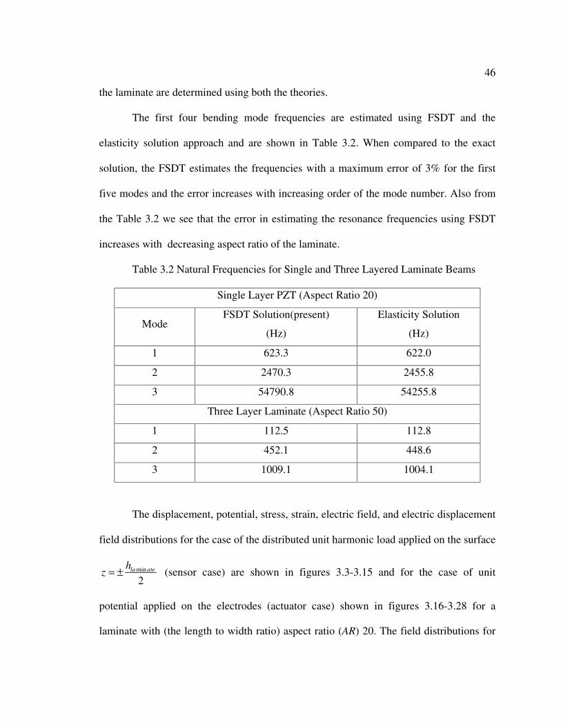
46
the laminate are determined using both the theories.
The first four bending mode frequencies are estimated using FSDT and the
elasticity solution approach and are shown in Table 3.2. When compared to the exact
solution, the FSDT estimates the frequencies with a maximum error of 3% for the first
five modes and the error increases with increasing order of the mode number. Also from
the Table 3.2 we see that the error in estimating the resonance frequencies using FSDT
increases with decreasing aspect ratio of the laminate.
Table 3.2 Natural Frequencies for Single and Three Layered Laminate Beams
Single Layer PZT (Aspect Ratio 20)
Mode FSDT Solution(present)
(Hz)
Elasticity Solution
(Hz)
1 623.3 622.0
2 2470.3 2455.8
3 54790.8 54255.8
Three Layer Laminate (Aspect Ratio 50)
1 112.5 112.8
2 452.1 448.6
3 1009.1 1004.1
The displacement, potential, stress, strain, electric field, and electric displacement
field distributions for the case of the distributed unit harmonic load applied on the surface
2min atelah
z ±= (sensor case) are shown in figures 3.3-3.15 and for the case of unit
potential applied on the electrodes (actuator case) shown in figures 3.16-3.28 for a
laminate with (the length to width ratio) aspect ratio (AR) 20. The field distributions for
47
the actuator case and sensor case for the laminate with aspect ratio of 50 are shown in
figures 3.29-3.54. The in-plane displacement, shear stress, shear strain, y component of
electric field and the y component of electric displacement shown in the figures 3.3–3.54
correspond to the edges of the beam, while the remaining fields are estimated at the mid-
span of the beam. The excitation frequency is 90% of the first resonance frequency for
both mechanical and electrical loading. The convergence of the Fourier series expansion
is checked before estimating fields.
From figures 3.3 to 3.4 we see that for AR = 20, FSDT predicts the in-plane
displacements and the transverse displacements with an error of 45 and 25 percent. The
error in estimating the potential (Fig. 3.5) is nearly 42 percent. The variation of potential
through the thickness is almost linear inside the sensor layer as estimated by the full
electroelasticity theory. The error in estimating the bending stress is 45 percent. The
FSDT estimates zero transverse normal stress, which is not true as shown by the elasticity
solution in figure 3.7. From figure 3.8, we see that the shear stress is constant inside the
layers in contrast to the nonlinear variation predicted by elasticity theory. The error in
estimating the bending strains using FSDT is the same as that in estimating the in-plane
displacement. Figure 3.12 and 3.13, shows the variation of y and z component of the
electric fields inside the layers. There is a large difference in the y component electric
field predicted by FSDT and elasticity theory. The zero y component electric
displacement and the constant shear strain assumption in the FSDT leads to a large error
in estimating the y component electric field inside the piezoelectric layers. Elasticity
theory predicts almost a zero y component electric field inside the layers which one

48
would have obtained if the Ey = 0 assumption is used instead of the Dy = 0 assumption.
There is a large error even in predicting the z component electric field inside a sensor by
FSDT for thick laminates, which is shown in figure 3.13. Both the y and z component of
the D field are not zero inside the sensor layers but have a very small value predicted by
elasticity theory in contrast to the zero y and z component D field predicted by FSDT.
Figures 3.16-3.28 show the electromechanical fields inside the laminate for
AR = 20 when a unit harmonic potential is applied on the outer surface electrodes of the
actuator layers. For this case also the fields estimated by the FSDT do not agree well with
those predicted by elasticity theory except for the potential and z component of the
electric field. This is because the first term in eqns (3.26) and (3.30) for electric potential
and electric fields inside the actuator layer is large when compared to the second term,
which results in a linear variation of potential through the thickness and constant Ez field
inside the actuator layers. The difference between the two estimates of in-plane and w
displacement by FSDT and elasticity theory is approximately 45 percent. There is a large
difference in the estimation of bending stress and bending strain values inside the layers
between the two theories. Figure 3.20 shows that even in the absence of an external
transverse load for the actuator case, the transverse normal stress inside the laminate is
nonzero which cannot be predicted by FSDT. As in the sensor case, the FSDT predicts a
nonzero Ey field inside the piezoelectric layers in contrast to the zero Ey value estimated
by elasticity theory. Elasticity theory predicts a nonzero Dy field inside the actuator layer.
For lower aspect ratio beams, AR=20 or less, from figures 3.3 through 3.28, we
see that FSDT cannot estimate the electromechanical fields accurately and the errors

49
involved in estimating the electrical fields are higher than the errors involved in the
mechanical fields.
Figures 3.29 through 3.54 show the variation of electromechanical fields for the
sensor and actuator cases inside the three layer laminate for AR= 50. For slender beams
the fields predicted by FSDT and elasticity theory agree well. In figures 3.31 and 3.39,
FSDT estimates the potential and Ez field inside the sensor layers with 30-35 percent
error even for the case of very thin laminates. The difference between the two estimates
of shear and transverse normal stresses and strains are due to the kinematic assumptions
made in FSDT. As in the previous case, the estimation of Ey by FSDT differs
considerably (fig. 3.38) from the values given by elasticity theory. This is due to the
constant shear strain assumption through the thickness of the laminate in FSDT and
neglecting Dy. Both mechanical and electrical fields inside a thin laminate estimated by
FSDT agree very well with that predicted by elasticity theory when a unit harmonic
potential is applied on the outer electrode surfaces of the actuator layers except for the Ey
field. The field distributions for the laminate with AR= 50 when a unit potential is applied
on the laminate surfaces (actuator case) are shown in figures 3.42-3.54. Here also the
FSDT is able to predict the fields inside the material and actuator layers accurately except
for Ey, Dy,, normal stress and strain fields due to assumptions made in FSDT as explained
before. Unlike the sensor case, for the actuator case, the FSDT is able to predict the
electrical potential and Ez field more accurately. If the actuator or sensor layers are thick
then we expect a quadratic variation of potential and linear variation of Ez field inside the
layers as suggested in (Yang, 1999).

50
3.6 Summary
The FSDT for the piezoelectric laminates is presented. The governing equations
for a piezoelectric laminate are derived using first order shear deformation laminated
beam theory and the solutions for the free and forced vibration problems of a simply
supported piezoelectric laminated beam are obtained using the derived formulations. For
the first time, the dynamic response fields inside the laminate obtained using FSDT are
compared with the corresponding fields obtained using three-dimensional elasticity
theory to bring out the effect of the kinematic and other assumptions made in FSDT. A
Fourier series solution method is employed to calculate the field distributions inside the
layers for the elasticity solution approach. For a thin laminate or a laminate with high
aspect ratio (AR=50), the electromechanical fields predicted by FSDT agree well with the
elasticity solution approach. But for the sensor case, the FSDT could not predict the
potential distribution inside the sensor layers accurately though it predicts the mechanical
fields with good accuracy. The assumption that Dy = 0, along with the constant shear
strain approximation introduces a large error in estimating the y component of the electric
field inside the piezoelectric layers. It is observed that the FSDT estimates a constant
electric displacement field inside the piezoelectric layer. This together with the reduced
charge equation and sensor boundary condition on the sensor electrodes forces the z
component of the electric displacement field to be zero everywhere inside the sensor
layer. For a better estimation of the electric displacement field, higher order laminated
theories without approximations to the charge equation are needed. This is needed
particularly when the strains induced in the piezoelectric layers are large. Though only a

51
three-layered symmetric laminate is considered for numerical calculations in the present
study, the approach presented here can be applied to a nonsymmetrical laminate with
multiple embedded piezoelectric layers.
When using FSDT to model a structure, careful consideration must be given not
only to the aspect ratio of the layers but also to the type of loads applied to the structure.
In active vibration and noise control, it is important to control the dominant modes of
vibration of the structure. It is seen from the present study that errors resulting from the
use of FSDT are magnified at such frequencies. In addition, one must also consider the
practicality of using piezoelectric layers that cover the entire structure. PVDF is the only
polymeric piezoelectric material in common use. However, it is not very efficient as an
actuator, particularly for the control of metallic plates. PZT is an efficient actuator
material, however it is very stiff and brittle and fabrication of laminates containing PZT
layers will be a challenge. Since both materials are poled, they cannot be subjected to
very high temperatures when fabricating the laminates to prevent depoling and loss of
piezoelectric properties. The originally designed structure will be changed drastically
after embedding the piezoelectric layers with respect to resonance frequencies and
dynamic response. For these reasons, laminates appear to be impractical for real
structures. The many research publications on piezoelectric laminates are a natural
extension of FSDT for composite laminates. However, the coupling of the electro-
mechanical fields result in large errors if thin plate theories are used. There appears to be
no simple analytical way to use FSDT for the case of discrete piezoelectric patches
applied to plate structures except as proposed by Kim and Varadan (Kim et al 1996).

52
They have proposed a finite element approach with transition elements to connect the
piezoelectric patch regions to the plate regions. It is hoped that the detailed analysis and
plots of all components of the mechanical and electric fields in the sensor and actuator
layers will be of use to researchers in this field.

53
-0.005
-0.004
-0.003
-0.002
-0.001
0.000
0.001
0.002
0.003
0.004
0.005
-1.500E-09 -1.000E-09 -5.000E-10 0.000E+00 5.000E-10 1.000E-09 1.500E-09
v Displacement (m)
z C
oo
rdin
ate
(m
)
3-D Elasticity
FSDT
-0.005
-0.004
-0.003
-0.002
-0.001
0.000
0.001
0.002
0.003
0.004
0.005
0.00E+00 2.00E-09 4.00E-09 6.00E-09 8.00E-09 1.00E-08 1.20E-08 1.40E-08
w displacement (m)
z c
oo
rdin
ate
(m
)
3-D Elasticity
FSDT
Figure 3.3 Axial Displacement (v) for Sensor Case (l/h = 20)
Figure 3.4 Transverse Displacement (w) for Sensor Case (l/h = 20)

54
-0.005
-0.004
-0.003
-0.002
-0.001
0.000
0.001
0.002
0.003
0.004
0.005
-2000 -1500 -1000 -500 0 500 1000 1500 2000
Bending Stress (pa)
z C
oo
rdin
ate
(m
)
3-D Elasticity
FSDT
-0.005
-0.004
-0.003
-0.002
-0.001
0.000
0.001
0.002
0.003
0.004
0.005
-0.007 -0.006 -0.005 -0.004 -0.003 -0.002 -0.001 0.000 0.001
Electr ic P otential (V)
z C
oo
rdin
ate
(m
)
3-D E las ticity
F S DT
Figure 3.6 Bending Stress (σy) for Sensor case (l/h = 20)
Figure 3.5 Electric Potential (φ) for Sensor case (l/h = 20)

55
-0.005
-0.004
-0.003
-0.002
-0.001
0.000
0.001
0.002
0.003
0.004
0.005
-0.60 -0.40 -0.20 0.00 0.20 0.40 0.60 0.80 1.00 1.20 1.40 1.60
Normal Stress (Pa)
z C
oo
rdin
ate
(m
)
3-D Elasticity
FSDT
-0.005
-0.004
-0.003
-0.002
-0.001
0.000
0.001
0.002
0.003
0.004
0.005
-50 0 50 100 150 200 250
Shear Stress (pa)
z C
oo
rdin
ate
(m
)
3-D Elasticity
FSDT
Figure 3.8 Shear Stress for Sensor case (l/h = 20)
Figure 3.7 Transverse Normal Stress for Sensor Case (l/h = 20)

56
-0 .005
-0 .004
-0 .003
-0 .002
-0 .001
0 .000
0 .001
0 .002
0 .003
0 .004
0 .005
-1 .0E-09 -8 .0E-10 -6 .0E-10 -4 .0E-10 -2 .0E-10 0 .0E+00 2 .0E-10 4.0E-10 6 .0E-10 8 .0E-10 1 .0E-09
Tra nsve rse no rm a l stra in
z C
oo
rdin
ate
(m
)
3-D E la stic ity
FSD T
-0.005
-0.004
-0.003
-0.002
-0.001
0.000
0.001
0.002
0.003
0.004
0.005
-2.0E-08 -1.5E-08 -1.0E-08 -5.0E-09 0.0E+00 5.0E-09 1.0E-08 1.5E-08 2.0E-08
Bending strain
z C
oo
rdin
ate
(m
)
3-D Elasticity
FSDT
Figure 3.10 Transverse normal strain for Sensor case (l/h = 20)
Figure 3.9 Bending strain for Sensor case (l/h = 20)

57
-0.005
-0.004
-0.003
-0.002
-0.001
0.000
0.001
0.002
0.003
0.004
0.005
-1.0 0.0 1.0 2.0 3.0 4.0 5.0 6.0 7.0
y Com ponent Electric Field (V/m)
z C
oo
rdin
ate
(m
)
3-D Elasticity
FSDT
-0.005
-0.004
-0.003
-0.002
-0.001
0.000
0.001
0.002
0.003
0.004
0.005
-2.0E-09 -1.0E-09 0.0E+00 1.0E-09 2.0E-09 3.0E-09 4.0E-09 5.0E-09 6.0E-09 7.0E-09
Shear strain
z C
oo
rdin
ate
(m
)
3-D Elasticity
FSDT
Figure 3.11 Shear strain for Sensor case (l/h = 20)
Figure 3.12 y Component of the Electric Field for Sensor Case (l/h = 20)
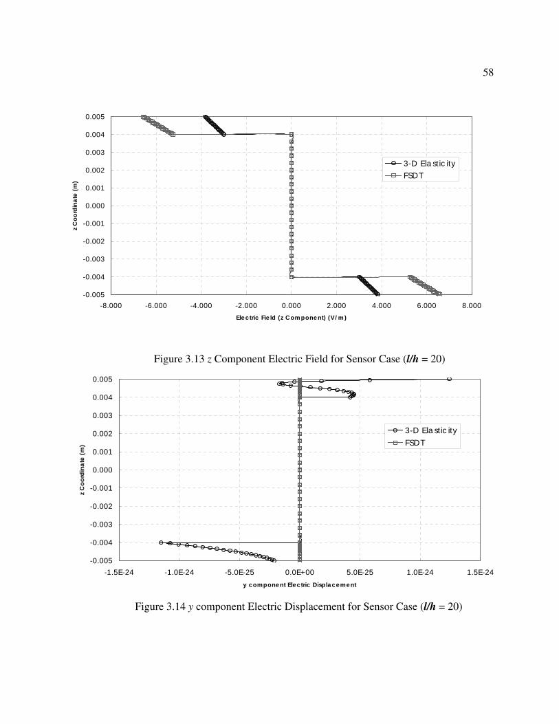
58
-0.005
-0.004
-0.003
-0.002
-0.001
0.000
0.001
0.002
0.003
0.004
0.005
-1.5E-24 -1.0E-24 -5.0E-25 0.0E+00 5.0E-25 1.0E-24 1.5E-24
y component Electric Displacement
z C
oo
rdin
ate
(m
)
3-D Elasticity
FSDT
-0.005
-0.004
-0.003
-0.002
-0.001
0.000
0.001
0.002
0.003
0.004
0.005
-8.000 -6.000 -4.000 -2.000 0.000 2.000 4.000 6.000 8.000
Electric Field (z Component) (V/m)
z C
oo
rdin
ate
(m
)
3-D Elasticity
FSDT
Figure 3.13 z Component Electric Field for Sensor Case (l/h = 20)
Figure 3.14 y component Electric Displacement for Sensor Case (l/h = 20)

59
-0.005
-0.004
-0.003
-0.002
-0.001
0.000
0.001
0.002
0.003
0.004
0.005
-8.0E-11 -6.0E-11 -4.0E-11 -2.0E-11 0.0E+00 2.0E-11 4.0E-11 6.0E-11 8.0E-11
z Component Electric Displacem ent (C/m ^2)
z C
oo
rdin
ate
(m
)
3-D Elasticity
FSDT
Figure 3.15 z component Electric Displacement for Sensor Case (l/h =20)

60
-0.005
-0.004
-0.003
-0.002
-0.001
0.000
0.001
0.002
0.003
0.004
0.005
-1.500E-08 -1.000E-08 -5.000E-09 0.000E+00 5.000E-09 1.000E-08 1.500E-08
v Displacement (m)
z C
oo
rdin
ate
(m
)
3-D Elasticity
FSDT
-0.005
-0.004
-0.003
-0.002
-0.001
0.000
0.001
0.002
0.003
0.004
0.005
0.00E+00 2.00E-08 4.00E-08 6.00E-08 8.00E-08 1.00E-07 1.20E-07 1.40E-07 1.60E-07
w displacement (m)
z c
oo
rdin
ate
(m
)
3-D Elasticity
FSDT
Figure 3.16 Axial Displacement for Actuator case (l/h = 20)
Figure 3.17 Transverse Displacement for Actuator Case (l/h = 20)

61
-0.005
-0.004
-0.003
-0.002
-0.001
0.000
0.001
0.002
0.003
0.004
0.005
-25000 -20000 -15000 -10000 -5000 0 5000 10000 15000 20000 25000
Bending Stress (pa)
z C
oo
rdin
ate
(m
)
3-D Elasticity
FSDT
-0.005
-0.004
-0.003
-0.002
-0.001
0.000
0.001
0.002
0.003
0.004
0.005
-1.200 -1.000 -0.800 -0.600 -0.400 -0.200 0.000 0.200
Electric Potential (V)
z C
oo
rdin
ate
(m
)
3-D Elasticity
FSDT
Figure 3.18 Electric Potential Actuator case (l/h = 20)
Figure 3.19 Bending Stress for Actuator case (l/h = 20)

62
-0.005
-0.004
-0.003
-0.002
-0.001
0.000
0.001
0.002
0.003
0.004
0.005
-15.00 -10.00 -5.00 0.00 5.00 10.00 15.00
Normal Stress (Pa)
z C
oo
rdin
ate
(m
)
3-D Elasticity
FSDT
-0.005
-0.004
-0.003
-0.002
-0.001
0.000
0.001
0.002
0.003
0.004
0.005
-500 -450 -400 -350 -300 -250 -200 -150 -100 -50 0 50
Shear Stress (pa)
z C
oo
rdin
ate
(m
)
3-D Elastic ity
FSDT
Figure 3.20 Transverse Normal Stress Actuator Case (l/h = 20)
Figure 3.21 Shear Stress for Actuator case (l/h = 20)

63
-0.005
-0.004
-0.003
-0.002
-0.001
0.000
0.001
0.002
0.003
0.004
0.005
-2.0E-07 -1.5E-07 -1.0E-07 -5.0E-08 0.0E+00 5.0E-08 1.0E-07 1.5E-07 2.0E-07
Bending strain
z C
oo
rdin
ate
(m
)
3-D Elasticity
FSDT
-0.005
-0.004
-0.003
-0.002
-0.001
0.000
0.001
0.002
0.003
0.004
0.005
-3.0E-07 -2.0E-07 -1.0E-07 0.0E+00 1.0E-07 2.0E-07 3.0E-07
Transverse normal strain
z C
oo
rdin
ate
(m
)
3-D Elasticity
FSDT
Figure 3.22 Bending strain for Actuator case (l/h = 20)
Figure 3.23 Transverse normal strain for Actuator case (l/h = 20)

64
-0.005
-0.004
-0.003
-0.002
-0.001
0.000
0.001
0.002
0.003
0.004
0.005
-14.0 -12.0 -10.0 -8.0 -6.0 -4.0 -2.0 0.0 2.0
y Component Electric Field (V/m)
z C
oo
rdin
ate
(m
)
3-D Elasticity
FSDT
-0.005
-0.004
-0.003
-0.002
-0.001
0.000
0.001
0.002
0.003
0.004
0.005
-3.0E-07 -2.0E-07 -1.0E-07 0.0E+00 1.0E-07 2.0E-07 3.0E-07
Shear strain
z C
oo
rdin
ate
(m
)
3-D Elasticity
FSDT
Figure 3.24 Shear strain for Actuator case (l/h = 20)
Figure 3.25 y Component Electric Field for Actuator case (l/h = 20)

65
-0.005
-0.004
-0.003
-0.002
-0.001
0.000
0.001
0.002
0.003
0.004
0.005
-5.E-19 -5.E-19 -4.E-19 -4.E-19 -3.E-19 -3.E-19 -2.E-19 -2.E-19 -1.E-19 -5.E-20 0.E+00 5.E-20
y component Electric Displacement
z C
oo
rdin
ate
(m
)
3-D Elasticity
FSDT
-0.005
-0.004
-0.003
-0.002
-0.001
0.000
0.001
0.002
0.003
0.004
0.005
-1500.000 -1000.000 -500 .000 0.000 500.000 1000.000 1500.000
Electric Fie ld (z C om ponent) (V /m )
z C
oo
rdin
ate
(m
) 3-D E la stic ity
FSD T
Figure 3.26 z Component Electric Field for Actuator case (l/h = 20)
Figure 3.27 y component of the Electric Displacement for Actuator case (l/h = 20)

66
-0.005
-0.004
-0.003
-0.002
-0.001
0.000
0.001
0.002
0.003
0.004
0.005
-2.0E-05 -1.5E-05 -1.0E-05 -5.0E-06 0.0E+00 5.0E-06 1.0E-05 1.5E-05 2.0E-05
z C om ponent E lectric D isp lacem ent (C /m ^2)
z C
oo
rdin
ate
(m
)
3-D E la stic ity
FSD T
-0.005
-0.004
-0.003
-0.002
-0.001
0.000
0.001
0.002
0.003
0.004
0.005
-2.000E-08 -1.500E-08 -1.000E-08 -5.000E-09 0.000E+00 5.000E-09 1.000E-08 1.500E-08 2.000E-08
v Displacement (m)
z C
oo
rdin
ate
(m
) 3-D Elasticity
FSDT
Figure 3.28 z Component Electric Displacement for Actuator case (l/h = 20)
Figure 3.29 Axial Displacement for Sensor case (l/h = 50)

67
-0.005
-0.004
-0.003
-0.002
-0.001
0.000
0.001
0.002
0.003
0.004
0.005
4.74E-07 4.75E-07 4.76E-07 4.77E-07 4.78E-07 4.79E-07 4.80E-07 4.81E-07 4.82E-07
w displacement (m)
z c
oo
rdin
ate
(m
)
3-D Elasticity
FSDT
Figure 3.30 Transverse Displacement for Sensor Case (l/h = 50)

68
-0.005
-0.004
-0.003
-0.002
-0.001
0.000
0.001
0.002
0.003
0.004
0.005
-15000 -10000 -5000 0 5000 10000 15000
Bending Stress (pa)
z C
oo
rdin
ate
(m
)
3-D Elasticity
FSDT
-0.005
-0.004
-0.003
-0.002
-0.001
0.000
0.001
0.002
0.003
0.004
0.005
-0.005 0.000 0.005 0.010 0.015 0.020 0.025 0.030 0.035 0.040
Electric Potentia l (V)
z C
oo
rdin
ate
(m
)
3-D Elastic ity
FSDT
Figure 3.31 Electric Potential for Sensor case (l/h = 50)
Figure 3.32 Bending Stress for Sensor case (l/h = 50)

69
-0.005
-0.004
-0.003
-0.002
-0.001
0.000
0.001
0.002
0.003
0.004
0.005
-1.5E-07 -1.0E-07 -5.0E-08 0.0E+00 5.0E-08 1.0E-07 1.5E-07
Bending strain
z C
oo
rdin
ate
(m
)
3-D Elasticity
FSDT
-0 .0 0 5
-0 .0 0 4
-0 .0 0 3
-0 .0 0 2
-0 .0 0 1
0 .0 0 0
0 .0 0 1
0 .0 0 2
0 .0 0 3
0 .0 0 4
0 .0 0 5
-1 0 0 0 1 0 0 2 0 0 3 0 0 4 0 0 5 0 0 6 0 0 7 0 0
Sh e a r S tre ss (p a )
z C
oo
rdin
ate
(m
)
3 -D E la st ic ity
FSD T
Figure 3.33 Bending strain for Sensor case (l/h = 50)
Figure 3.34 Shear Stress for Sensor case (l/h = 50)

70
-0 .0 0 5
-0 .0 0 4
-0 .0 0 3
-0 .0 0 2
-0 .0 0 1
0 .0 0 0
0 .0 0 1
0 .0 0 2
0 .0 0 3
0 .0 0 4
0 .0 0 5
-2 .0 0 -1 .5 0 -1 .0 0 -0 .5 0 0 .0 0 0 .5 0 1 .0 0
N o rm a l S tre s s (P a )
z C
oo
rdin
ate
(m
)
3 -D E la s t ic ity
F S D T
-0.005
-0.004
-0.003
-0.002
-0.001
0.000
0.001
0.002
0.003
0.004
0.005
-8.0E-09 -6.0E-09 -4.0E-09 -2.0E-09 0.0E+00 2.0E-09 4.0E-09 6.0E-09 8.0E-09
Transverse normal strain
z C
oo
rdin
ate
(m
)
3-D Elasticity
FSDT
Figure 3.35 Transverse Normal Stress for Sensor Case (l/h = 50)
Figure 3.36 Transverse normal strain for Sensor case (l/h = 50)

71
-0 .005
-0.004
-0.003
-0.002
-0.001
0.000
0.001
0.002
0.003
0.004
0.005
-2.0 0.0 2.0 4 .0 6.0 8.0 10.0 12.0 14.0 16.0
y C om ponent E lec tric F ie ld (V/m )
z C
oo
rdin
ate
(m
)
3-D E la stic ity
FSD T
-0.005
-0.004
-0.003
-0.002
-0.001
0.000
0.001
0.002
0.003
0.004
0.005
-1.0E-08 -5.0E-09 0.0E+00 5.0E-09 1.0E-08 1.5E-08 2.0E-08
Shear strain
z C
oo
rdin
ate
(m
)
3-D Elasticity
FSDT
Figure 3.37 Shear strain for Sensor case (l/h = 50)
Figure 3.38 y Component Electric Field for Sensor case (l/h = 50)

72
-0.005
-0.004
-0.003
-0.002
-0.001
0.000
0.001
0.002
0.003
0.004
0.005
-5.0E-09 0.0E+00 5.0E-09 1.0E-08 1.5E-08 2.0E-08 2.5E-08 3.0E-08
y com ponent E lectric D isp lacem ent
z C
oo
rdin
ate
(m
)
3-D E la stic ity
FSD T
-0.005
-0.004
-0.003
-0.002
-0.001
0.000
0.001
0.002
0.003
0.004
0.005
-50.000 -40.000 -30.000 -20.000 -10.000 0.000 10.000 20.000 30.000 40.000 50.000
Electric Field (z Component) (V/m)
z C
oo
rdin
ate
(m
)
3-D Elasticity
FSDT
Figure 3.39 z Component Electric Field for Sensor case (l/h = 50)
Figure 3.40 y component Electric Displacement for Sensor case (l/h = 50)

73
-0.005
-0.004
-0.003
-0.002
-0.001
0.000
0.001
0.002
0.003
0.004
0.005
-1.E-10 -8.E-11 -6.E-11 -4.E-11 -2.E-11 0.E+00 2.E-11 4.E-11 6.E-11 8.E-11 1.E-10
z Component Electric Displacement (C/m^2)
z C
oo
rdin
ate
(m
)
3-D Elasticity
FSDT
-0.005
-0.004
-0.003
-0.002
-0.001
0.000
0.001
0.002
0.003
0.004
0.005
-4.000E-08 -3.000E-08 -2.000E-08 -1.000E-08 0.000E+00 1.000E-08 2.000E-08 3.000E-08 4.000E-08
v Displacement (m)
z C
oo
rdin
ate
(m
)
3-D Elasticity
FSDT
Figure 3.41 z Component Electric Displacement for Sensor case (l/h = 50)
Figure 3.42 Axial Displacement for Actuator case (l/h = 50)

74
-0.005
-0.004
-0.003
-0.002
-0.001
0.000
0.001
0.002
0.003
0.004
0.005
8.90E-07 8.91E-07 8.92E-07 8.93E-07 8.94E-07 8.95E-07 8.96E-07 8.97E-07 8.98E-07 8.99E-07 9.00E-07 9.01E-07
w displacement (m)
z c
oo
rdin
ate
(m
)
3-D Elasticity
FSDT
-0.005
-0.004
-0.003
-0.002
-0.001
0.000
0.001
0.002
0.003
0.004
0.005
-0.200 0.000 0.200 0.400 0.600 0.800 1.000 1.200
Electric Potential (V)
z C
oo
rdin
ate
(m
)
3-D Elasticity
FSDT
Figure 3.44 Electric Potential for Actuator case (l/h = 20)
Figure 3.43 Transverse Displacement for Actuator Case (l/h = 50)

75
-0.005
-0.004
-0.003
-0.002
-0.001
0.000
0.001
0.002
0.003
0.004
0.005
-20000 -15000 -10000 -5000 0 5000 10000 15000 20000
Bending Stress (pa)
z C
oo
rdin
ate
(m
) 3-D Elasticity
FSDT
-0.005
-0.004
-0.003
-0.002
-0.001
0.000
0.001
0.002
0.003
0.004
0.005
-3.00 -2 .00 -1 .00 0.00 1.00 2.00 3.00 4.00
N orm al Stress (Pa)
z C
oo
rdin
ate
(m
)
3-D E la stic ity
FSD T
Figure 3.45 Bending Stress for Actuator case (l/h = 50)
Figure 3.46 Transverse Normal Stress for Actuator Case (l/h = 50)

76
-0.005
-0.004
-0.003
-0.002
-0.001
0.000
0.001
0.002
0.003
0.004
0.005
-2.0E-07 -1.5E-07 -1.0E-07 -5.0E-08 0.0E+00 5.0E-08 1.0E-07 1.5E-07 2.0E-07
Bending strain
z C
oo
rdin
ate
(m
)
3-D Elasticity
FSDT
-0.005
-0.004
-0.003
-0.002
-0.001
0.000
0.001
0.002
0.003
0.004
0.005
-1000 -500 0 500 1000 1500
Shear Stress (pa)
z C
oo
rdin
ate
(m
)
3-D Elasticity
FSDT
Figure 3.47 Shear Stress for Actuator case (l/h = 50)
Figure 3.48 Bending strain for Actuator case (l/h = 50)

77
-0.005
-0.004
-0.003
-0.002
-0.001
0.000
0.001
0.002
0.003
0.004
0.005
-3.0E-07 -2.0E-07 -1.0E-07 0.0E+00 1.0E-07 2.0E-07 3.0E-07
Transverse normal strain
z C
oo
rdin
ate
(m
)
3-D Elasticity
FSDT
-0.005
-0.004
-0.003
-0.002
-0.001
0.000
0.001
0.002
0.003
0.004
0.005
-3.0E-07 -2.0E-07 -1.0E-07 0.0E+00 1.0E-07 2.0E-07 3.0E-07
Shear strain
z C
oo
rdin
ate
(m
)
3-D Elasticity
FSDT
Figure 3.49 Transverse normal strain for Actuator case (l/h = 50)
Figure 3.50 Shear strain for Actuator case (l/h = 50)

78
-0.005
-0.004
-0.003
-0.002
-0.001
0.000
0.001
0.002
0.003
0.004
0.005
-1800.0 -1600.0 -1400.0 -1200.0 -1000.0 -800.0 -600.0 -400.0 -200.0 0.0 200.0
y Component Electric Field (V/m)
z C
oo
rdin
ate
(m
) 3-D Elasticity
FSDT
-0.005
-0.004
-0.003
-0.002
-0.001
0.000
0.001
0.002
0.003
0.004
0.005
-1500.000 -1000.000 -500.000 0.000 500.000 1000.000 1500.000
Electric Field (z Component) (V/m)
z C
oo
rdin
ate
(m
)
3-D Elasticity
FSDT
Figure 3.51 y Component Electric Field for Actuator case (l/h = 50)
Figure 3.52 z Component Electric Field for Actuator case (l/h = 50)

79
-0.005
-0.004
-0.003
-0.002
-0.001
0.000
0.001
0.002
0.003
0.004
0.005
-5.E-06 0.E+00 5.E-06 1.E-05 2.E-05 2.E-05 3.E-05 3.E-05 4.E-05
y component Electric Displacement
z C
oo
rdin
ate
(m
)
3-D Elasticity
FSDT
-0.005
-0.004
-0.003
-0.002
-0.001
0.000
0.001
0.002
0.003
0.004
0.005
-2.0E-05 -1.5E-05 -1.0E-05 -5.0E-06 0.0E+00 5.0E-06 1.0E-05 1.5E-05 2.0E-05
z Component Electric Displacement (C/m^2)
z C
oo
rdin
ate
(m
) 3-D Elasticity
FSDT
Figure 3.53 y component Electric Displacement for Actuator case (l/h = 50)
Figure 3.54 z Component Electric Displacement for Actuator case (l/h = 50)

80
Chapter 4 MODELING OF VIBRATION AND NOISE CONTROL USING DISCRETE PIEZOELECTRIC ACTUATORS/SENSORS -a) Fourier series method b) Rayleigh-Ritz approach
4.1 Introduction
Surface bonded discrete piezoelectric patches for plates and shell structures have
proven to be an efficient and simple approach to actively control vibration and radiated
noise. By proper placement, distributed sensors can be used to sense membrane response
or bending response or both. The sensing and actuation effects of distributed piezoelectric
sensors and actuators depend on their shape, thickness, material properties, placement,
spatial shaping and spatial distribution. When a single piece fully distributed piezoelectric
sensor/actuator is used there are observability and controllability deficiencies in
monitoring and control of plates and shells (Tzou 1993). Spatial shaping of distributed
sensors and actuators, for example by segmenting them into a number of smaller pieces,
can improve the controllability and observability. The effectiveness of distributed
piezoelectric sensors and actuators, in the form of rectangular patches, bonded on simply
supported rectangular thin composite plates and circular cylindrical shell panels have
been investigated by Tzou and Fu (1994a,b). When the piezoelectric patches are surface
bonded to the plate structure, the presence of a patch can affect the dynamic
characteristics of the host structure in two ways (Banks et al 1995). The fact that the
patch has a definite thickness and material properties, the contribution of the patch
stiffness and mass to the host structures stiffness and mass changes the global dynamic

81
behavior of the smart plate. This leads to additional terms in the force and moment
resultant of the host plate that must be estimated accurately in order to predict the
dynamic characteristics of the smart plate like frequencies and mode shapes. The other
contribution is due to the application of voltages (active stiffness) on the electrodes of the
actuator, which generates the moments and forces which appear as forcing functions in
the final dynamic equations of motion. In all earlier models the mass and stiffness
contributions from sensor and actuator patches were neglected for estimating the natural
frequencies of the smart plate. Also the thickness direction electric fields and strain fields
inside the patches are assumed to be constant over the entire area of the patch. The
validity of these assumptions depends on the size and relative stiffness of the patches and
has not been investigated before. In this section, the Classical (Kirchoff’s) Plate Theory
(CPT) is used to estimate the natural frequencies of a plate structure with surface bonded
piezoelectric patches without the above-mentioned assumptions. A detailed modeling of
the patches is developed by expressing the electric potential inside the patch as a
quadratic function of the thickness coordinate. The equations of motion are derived for a
generally isotropic plate with surface bonded discrete patches. The solution to the
dynamic equations of motion is obtained using a Fourier series method for a plate with
collocated piezoelectric actuator/sensor patches. The effect of the passive stiffness of the
surface bonded actuator and sensor patches on the dynamic characteristics of host plate
structure is investigated.
In the present formulation the piezoelectric patch model is refined using the
electroelastic theory and by satisfying the charge equation. Also the contributions from

82
the discrete patches to a host plate are added and the effect of these contributions on the
dynamic characteristics of the smart plate is studied. Though the model development is
based on CPT this can be easily extended to FSDT and higher order plate theories
depending on geometric and material properties. This is one of the powerful features of
this formulation and also can be extended to shells.
Using the CPT model developed, a vibroacoustic model for studying the active
control of noise transmitted into a rectangular enclosure using discrete piezoelectric
patches is developed using the Rayleigh-Ritz (RR) method. The enclosure has five rigid
walls and a flexible smart plate, which is embedded with discrete piezoelectric actuators
and sensors. Eigenfunctions of a clamped-clamped beam are used as the Ritz functions
for the panel and the rigid-walled cavity modes are used to model the acoustic cavity. The
dynamic equations of motion for the coupled smart panel-cavity system are derived using
Hamilton’s principle. The forcing term due to the acoustic pressure in the cavity is
determined by using virtual work considerations. For the present study, five collocated
pairs of actuator/sensor are attached to the plate at predetermined positions. The results
obtained using the Rayleigh-Ritz procedure for a smart aluminum panel-cubic cavity is
compared with finite element (FE) and experimental results. Close agreement between
the present approach and the FE and experimental results confirms the validity of the
results. The RR method is suggested for the modeling of laboratory smart structures as an
alternative to the FE method because it provides the same accuracy with significant
reduction in computational size and time.

83
4.2 Piezoelectric Patches: Modeling And Formulation
Figure 4.1 shows a rectangular laminate on which piezoelectric patches are
bonded. The length and width of the each patch are ‘a’ and ‘b’. Lx and Ly are the
dimensions of the laminate.
The piezoelectric patches are polarized in the thickness direction and the major
surfaces are covered with electrodes of negligible thickness. The laminate is assumed to
lie on the z = 0 plane. The classical laminated plate theory, which is an extension of
Kirchoff’s (classical) plate theory to laminated composite plates assume the following
displacement fields:
Figure 4.1 Configuration of surface bonded piezoelectric patch
y
x
z
Lx
Ly
y2
b
x2
x1
y1
a h

84
, ),,(),,,(
and , ),,(),,,(
, ),,(),,,(
0
00
00
tyxwtzyxw
y
wztyxvtzyxv
x
wztyxutzyxu
=∂∂−=
∂∂−=
(4.1)
where u, v, w are the displacements along the x, y, z coordinate directions, respectively, of
a point on the midplane (i.e., z = 0). Kirchoff’s assumption amounts to neglecting both
transverse shear and transverse normal effects, i.e., deformation is entirely due to bending
and in-plane stretching. This leads to zero transverse strain components ),,( yzxzxx γγε .
Thus for small strains and moderate rotations the strain-displacement relations take the
form
, 2
and ,
,
02
00
20
20
20
20
yx
wz
x
v
y
u
y
wz
y
v
x
wz
x
u
x
y
x
∂∂∂−
∂∂+
∂∂=
∂∂−
∂∂=
∂∂−
∂∂=
γ
ε
ε
(4.2)
or shortly )1()0( εεε z+= ,
where
∂∂+
∂∂
∂∂∂∂
=
=
x
v
y
uy
vx
u
xy
xx
xx
00
0
0
)0(
)0(
)0(
)0(
γεε
ε and
∂∂∂−
∂∂−
∂∂−
=
=
yx
wy
wx
w
xy
xx
xx
02
20
2
20
2
)1(
)1(
)1(
)1(
2γεε
ε .
The linear constitutive relations for the host laminate in the principal material directions

85
are
)()(
662616
262221
161211
)( k
xy
yy
xx
kk
xy
yy
xx
QQQ
QQQ
QQQ
=
γεε
τσσ
,
where )(k
ijQ are the transformed stiffness coefficients. The linear constitutive relations
written in terms of nonzero stress and strain components for the attached piezoelectric
patches are
,
00
00
00
0
000
000
and ,
000
00
00
00
0
0
)(),(
)(),(33
)(),(22
)(),(11
)(),(
)(),(23
)(),(13
)(),(
)(),(
)(),(23
)(),(13
)(),(
)(),(66
)(),(22
)(),(12
)(),(12
)(),(11
)(),(
sa
z
y
x
sa
sa
sasa
xy
yy
xx
sasa
sa
z
y
x
sa
z
y
x
sa
sasa
xy
yy
xx
sa
sasa
sasasa
xy
yy
xx
E
E
E
eeD
D
D
E
E
E
e
e
C
CC
CC
∈∈
∈+
=
−
=
γεε
γεε
τσσ
(4.3)
where )(),( saijC , )(),( sa
ije and )(),( saii∈ are the stiffness coefficients at constant electric field,
piezoelectric constants and dielectric permittivities at constant state of stress of the
actuator and sensor patches. σi and Di are the stress and electric displacement
components. The superscripts (a) and (s) refer to the actuator and sensor patches. Apart
from satisfying the equilibrium equations the piezoelectric patch regions should satisfy
the charge equation 0=∇ • D . If the patches are thin, we can assume that the x and y
component electric displacement fields are constant along x and y directions within the
patch so that the charge equation reduces to 0=dz
dDz .

86
4.2.1 Actuator Patch Model
The electric potential inside the actuator patch (φa) is assumed to vary
quadratically along the thickness direction as:
aaaa zz 22
10 φφφφ ++= . (4.4)
It is assumed, that for the actuator patches the electrodes located at the laminate
patch interface (i.e., @ z=z1) are always grounded and a potential of Va is applied at the
other electrode surface (i.e., @ z=z0). Using these conditions in equation (4.4) we obtain
amaa
aa h
h
V21 2 φφ −= (4.5)
where ha = (z0- z1) is the thickness of the actuator patch and 2
)z +(z = h 10a
m is the distance
of the actuator middle surface from the laminate middle surface. Using the constitutive
equation and the reduced charge equation we obtain
( ) )()1()1(
33
312 2
a
yyxxa e εεφ +
∈−= . (4.6)
From equations (4.4), (4.5) and (4.6) the electric potential and electric field inside
the actuator patch is:
( ) )()1()1(
3331
a
yyxx
am
a
aaaz
hze
h
V
dz
dE εεφ +
∈−+−=−= . (4.7)
Substituting equation (4.7) into equation (4.3a) we obtain the stress-strain relation
for the actuator patches:

87
( )( )( )( )
.
and ,
,
)(66
)()1()1(
33
23131
2212
)()1()1(
33
23131
1211
axy
axy
a
yyxx
am
a
aayy
aaxx
aayy
a
yyxx
am
a
aayy
aaxx
aaxx
C
hze
h
VeCC
hze
h
VeCC
γτ
εεεεσ
εεεεσ
=
+∈−+++=
+∈−+++=
(4.8)
The above constitutive relations are valid only inside the actuator patches.
4.2.2 Sensor Patch Model
From the reduced charge equation, we observe that the z component electric
displacement should be constant along the thickness (z) direction of the sensor patch.
Also for the sensor there is no external supply of charge into the patch, so the total charge
that appears on the sensor patch electrode surfaces should be zero. This condition for the
present case can be written as 1+==
−=nn zzzzzz DD . This condition along with the reduced
charge equation forces Dz to be zero everywhere inside the patch. So from equation
(4.3b) we find
( ) ( ) ( ) )()1()1()()0()0(
33
31)(
33
31 s
yyxx
s
yyxxs
yyxxsz z
eeE εεεεεε +++
∈−=+
∈−= . (4.9)
If the electric potential inside the sensor patch is also assumed to vary
quadratically with z then we write:
ssss zz 22
10 φφφφ ++= . (4.10)
The electric field inside the patch is then obtained as
sss
sz z
dz
dE 21 2 φφφ −−=−= . (4.11)
Comparing equations (4.9) and (4.11) we obtain

88
( ) ( ))1()1(
33
312
)0()0(
33
311 2
; yyxxs
yyxxs ee εεφεεφ +
∈−=+
∈−= .
The average sensor potential (i.e., the voltage that appears between the sensor
electrodes is
( ) ( ) ∫∫ +−+∈
=
−=== As syyxx
smyyxx
s
s
Aszz
s
zz
s
s
s dAhA
ehdA
AV )1()1()0()0(
33
31
23
1 εεεεφφ (4.12)
where hs = (zn+1- zn) is the thickness of the sensor patch and 2
) +(h n1+ns
m
zz= is the
distance of the sensor patch middle surface from the laminate middle surface.
Substituting equation (4.11) in (4.3a) the stress-strain relation for the sensor patch is
obtained as:
.
and ,
,
66
33
2
2233
2
21
33
2
1233
2
11
3131
3131
sxy
sxy
syy
sxx
syy
syy
sxx
sxx
C
eC
eC
eC
eC
γτ
εεσ
εεσ
=
∈
−+
∈
−=
∈
−+
∈
−=
(4.13)
4.3 Smart Plate Model
The equilibrium equations for the plate with actuator and sensor patches bonded
on the surface are given as:

89
, ),,(2
and ,
,
2
2
2
22
2
2
2
2
2
2
tyxqt
wh
y
M
yx
M
x
M
t
vh
y
N
x
N
t
uh
y
N
x
N
yxyx
yxy
xyx
−=++
=+
=+
∂∂ρ
∂∂
∂∂∂
∂∂
∂∂ρ
∂∂
∂∂
∂∂ρ
∂∂
∂∂
(4.14)
where
dzRdzRdz
N
N
Nn
nn
z
zsxy
syy
sxx
z
zaxy
ayy
axx
z
zExy
Eyy
Exx
xy
y
x
∫∫∫ +
+
+
=
10
1
1
τσσ
τσσ
τσσ
(4.15)
are the membrane force resultants. Here Eiiσ are the stress components for the host plate
and R is the location function defined as
, elsewhere,0
and , ,,1
, )]()()][()([),(
=≤≤−≤≤−=
+−−+−−=bybaxa
ayHayHaxHaxHyxR
(4.16)
in which H is Heaviside function. The moment resultants Mi are defined as
dzzRdzzRdzz
M
M
Mn
nn
z
zsxy
syy
sxx
z
zaxy
ayy
axx
z
zExy
Eyy
Exx
xy
y
x
∫∫∫ +
+
+
=
10
1
1
τσσ
τσσ
τσσ
. (4.17)
The local mass density function ρ is defined as Rhhh aaaaEE )( )()()()( ρρρρ ++= ,
where )()( and sa ρρ are the mass densities of the sensor and actuator patch materials and
Eρ is the density of the host plate. Here q is the distributed harmonic load acting on the
plate surface. Substituting the stress-strain relations for the plate, actuator and sensor

90
patches from equations (4.8), (4.13) and (4.15) into the force and moment resultant
equations we obtain
[ ] [ ] [ ] [ ] [ ] [ ] [ ]
[ ] [ ] [ ] [ ] [ ] [ ] [ ] and ,I
, I
31)1()0()1()0()1()0(
31)1()0()1()0()1()0(
am
as
ss
sa
aa
a
as
ss
sa
aa
a
hVe
Ve
++++++=
++++++=
εεεεεε
εεεεεε
DBDBDBM
BABABAN
(4.18)
. ))((3
1;)(
3
1;)()(
and , )(;;)()(2
1
, )(;);()( where
31
3
33
2313
133
13
1
33
2312
12
1
33
231
11
Rzze
CDRzzCDzzQD
Rhhe
CBRhhCBzzQB
Rhe
CARhCAzzQA
aasij
sijaa
aij
aijkk
n
kkijij
sm
ssij
sij
am
aaij
aijkk
n
kkijij
ssij
sij
aaij
aijkk
n
kkijij
−−−=
−=
−=
−∈
+=−=−=
∈+==−=
∈+==−=
∑
∑
∑
and [I] is the identity matrix. Substituting the force and moment resultants (4.18) into the
plate equilibrium equation (4.14) we obtain the equation of motion for the smart plate.
For a square isotropic plate with collocated actuator/sensor patches the general equation
of motion reduces to
)2(])()([
)1(2
22
)(2
2
2
2)(
33
31
2
2
2
2
2
2
2
2
2
3
3
2
3
2
3
3
3
)(),(4
4
22
4
4
4
2
24
xyyyxxss
ms
s
sm
am
s
xy
i
yy
i
xx
i
y
i
x
ii
sai
i
RRRy
w
x
wh
y
v
x
uhhhe
Ryx
wR
y
w
x
wR
y
w
x
w
Ry
w
yx
wR
yx
w
x
wR
y
w
yx
w
x
wD
t
wwD
++∂∂+
∂∂+
∂∂+
∂∂
∈+
∂∂
∂−+
∂∂+
∂∂+
∂∂+
∂∂+
∂∂+
∂∂∂+
∂∂
∂+∂∂+
∂∂+
∂∂∂+
∂∂+
∂∂=∇−
∑=
G
ννν
ρ
(4.19)

91
whereyx
RR
y
RR
x
RR
y
RR
x
RR xyyyxxyx ∂∂
∂=∂∂=
∂∂=
∂∂=
∂∂=
2
2
2
2
2
and ,,,, . The first derivatives of R
correspond to the delta functions ( ii i
RR δ=
∂∂= ) in x and y directions and these exist
inside the integrals.
It should be noted that while deriving the above equation of motion for the plate
no assumptions are made on the strain fields other than the basic assumptions of CPT.
The terms inside the curly braces on the RHS of the above equations are due to the
passive stiffnesses of the actuator and sensor patches. If the strains are assumed to be
constant inside the patches then all these terms will vanish (B T Wang et al 1991, Tzou et
al 1994a, 1994b). In equation (4.19) the actuator voltage Va is replaced by feedback
voltage G Vs, where G is the feedback gain and Vs is the sensor output signal that is fed
back to the actuator.
4.4 Solution Method
To obtain the natural frequency of the smart plate the feedback gain is considered
to be zero. The solution for the equation (4.19) can be obtained by expanding the
displacement in a Fourier series. Assuming a double Fourier sine series for the lateral
displacement ‘w’ as ∑∑=m n
ti
yxmn e
l
yns
l
xmsAw ωππ
)(in)(in the equation of motion for the
smart plate reduces to

92
; )(in)(in
)(os)(cos)1(2
))cos()(in)(sin)(os(2
)(in)(sin)(
)),(( )),((
2
)),((6
)),((54
32)),((
1
∑∑ ∑ ∑
∑∑ ∑
∑∑ ∑
∑∑ ∑
= =
=
=
=
+−=
−−
++
−−+−
m n sai yxmn
sai
iii
m n yxmn
ixy
sai
i
m n sai yxmn
iy
i
ymn
x
ix
i
m n yxmn
iyy
iixx
ii
sai
i
l
yns
l
xmsARhh
l
ync
l
xmARI
l
yn
l
xmsARI
l
ynA
l
xmcRI
l
yns
l
xmARIRIRII
ππρρω
ππν
ππππ
ππ
(4.20)
where
222
+
=
yx l
n
l
mDI
ππ, ,,
22
2
222
1
+
=
+
=
yx
ii
yx
ii
l
n
l
mDI
l
n
l
mDI
πνπππ
. and ,
, ,
2
6
3
2
32
5
2
323
4
22
3
=
+
=
+
=
+
=
yx
ii
yyx
ii
yxx
ii
yx
ii
ll
mnDI
l
n
ll
nmDI
ll
mn
l
mDI
l
n
l
mDI
πππ
ππππν
The natural frequencies and the mode shapes of the plate cannot be obtained
directly from the above equation. So the modal method is used to estimate the
frequencies of the plate. Multiplying both sides of equation (4.20) by
)(in)(sinyx l
yqs
l
xp ππwhere p = 1,2, … r and q = 1,2, … s and integrating over the area of
the plate we can generate a system of equations for the various values of p and q.
Truncating the series at some values of m and n, we can write the system of equations in

93
matrix form as
[ ] [ ] AMAK 2ω−= . (4.21)
Solution to the above Eigenvalue problem gives the natural frequency pqω and
the coefficients Amn. The accuracy of the solution can be improved by considering more
terms in the series.
4.5 Results And Discussion
An aluminum plate with one pair of collocated piezoelectric sensor/actuator
patches (case I) and a Plexiglas plate with a one pair of PVDF patches (case II) are
considered for the present study. The properties of the plate and the piezoelectric patches
are given in Table 4.1.
Table 4.1 Material Properties for the plate and piezoelectric patches
Properties Host Plate PZT Host Plate PVDF
Youngs Modulus (E) N/m2 12.6e10 12.6e10 3.10e3 2.0e9
Density (ρ) Kg/m3 2800 7500 1190 1800
Thickness (h) m 1.0e-3 0.8e-3 1.6e-3 0.5e-3
Poission’s Ratio (ν) 0.3 0.2 0.35 0.2
Piezoelectric Constant (e31) N/Vm
- -0.52 - -0.13
Size m × m 0.305 × 0.305 Variable 0.2 × 0.2 Variable
The convergence of each natural frequency value is confirmed by considering
more terms in the series. Figure 4.2 shows the convergence of the first four natural

94
frequencies for a single pair of actuator/sensor for case I (patch size = 0.1 × 0.1 m) with
number of terms in the series. Table 4.2 shows the difference between the estimated
frequencies of the host plate alone and the plate with the collocated actuator/sensor
patches.
Table 4.2 Natural frequencies of the smart plate Case I (Hz) Case II (Hz)
Mode Plate Plate
With Patch Difference Plate
Plate With Patch
Difference
(1,1) 62.51 62.80 (0.5 %) 40.57 41.58 (4.0 %)
(1,2) 156.26 156.51 (0.3 %) 101.42 104.52 (3.9 %)
(1,3) 312.54 312.84 (0.1 %) 202.84 207.92 (2.5 %)
0
200
400
600
800
1000
1200
1400
0 20 40 60 80 100 120 140 160 180 200Total Number of Terms in the Fourier Series
Freq
uenc
y (H
z)
mode (1,1)
mode (1,2)
mode (1,3)
mode (1,4)
Figure 4.2 Convergence of the frequencies

95
0
1 0 0
2 0 0
3 0 0
4 0 0
5 0 0
6 0 0
0 .0 0 0 .0 3 0 .0 6 0 .0 9 0 .1 2 0 .1 5 0 .1 8 0 .2 1
S iz e o f th e P a tc h ( 2 a o r 2 b ) ( m )
Res
onan
t Fre
quen
cies
(H
z)
M o d e ( 1 ,1 )M o d e ( 1 ,2 )M o d e ( 2 ,2 )M o d e ( 2 ,3 )M o d e ( 3 ,3 )
Figure 4.3 Variation of the resonant frequencies with patch size for PVDF/Plexiglas/PVDF
Figure 4.4 Variation of the resonant frequencies with patch size for PZT/Al/PZT
0
2 0 0
4 0 0
6 0 0
8 0 0
1 0 0 0
1 2 0 0
1 4 0 0
0 .0 1 0 .0 4 0 .0 6 0 .0 9 0 .1 1 0 .1 4 0 .1 6 0 .1 9 0 .2 1 0 .2 4 0 .2 6 0 .2 9
S ize o f th e ac tu a to r/S en so r p a tch (’2 a ’ o r ’2 b ’) (m )
Res
onan
t Fre
quen
cies
(H
z)
M o d e (1 ,1 )
M o d e (2 ,2 )
M o d e (2 ,3 )
M o d e (3 ,3 )

96
The patch covers 10% of the host plate area. From Table 4.2, we observe that the
error due to neglecting the passive stiffness and mass of the patch is more pronounced for
a smart plate with PZT patch on aluminum plate than a PVDF patch on Plexiglas. The
stiffness and mass ratios of the host plate to patch materials; piezoelectric coupling
coefficient and size of the patches are the important factors, which decide the amount of
shift in the resonant frequencies of the host plate.
The effect of the patch size on the resonant frequencies can be seen from figures
4.3 and 4.4. Solving equation (4.20) with the active stiffness (i.e. due to either voltage
excitation or closed loop feedback) is extremely difficult, because of the non-orthogonal
nature of the assumed solution in the patch region (-a<x<a,-b<y<b).
4.6 Active Enclosure Noise Control using Rayleigh-Ritz Method
From the previous section we noticed, though we could derive the equation of
motion for surface bonded discrete actuators and sensors, it is nearly impossible to obtain
a solution for the forced vibration or feedback case. So a more powerful numerical
method should be considered for solving this problem.
A significant amount of scientific literature has been published on modeling the
smart panel systems using analytical and finite element methods. Although these earlier
FE models predict the behavior of the structural panel and the fluid-structure interaction
(in the case of active noise control system designs) accurately at low frequencies, at high
frequencies the size of the model increases resulting in very long computational time.
Furthermore, optimal actuator/sensor placement studies involve repeated and time-

97
consuming FE remeshing during the iterations. Thus, a closed form solution approach is
preferred over the FE method. In the following sections an energy approach based on the
Rayleigh-Ritz approach is presented. The formulation is presented for a smart panel
backed cavity to demonstrate the fact that this approach is not just for smart structures,
but could also be used for vibroacoustic systems with smart walls.
4.7 Potential And Kinetic Energies Of The System
4.7.1 Composite Plate
Using classical thin plate theory, the bending strain energy for a symmetrically
layered composite panel is given by
∫ ∫ ∫−=lx ly h
h
tplatew dzdydxU
0 0
2/
2/2
1. (4.22)
Substituting the expressions for the stresses and strains we obtain the strain
energy for the plate as
, 422
662
2
2
2
22
0 0 2
2
2
2
2
2
2
2
122
2
2
2
11
dydxyx
w
yx
wD
y
w
y
wD
x
w
y
w
y
w
x
wD
x
w
x
wDU
lx lyplatew
∂∂
∂∂∂
∂+
∂∂
∂∂+
∂∂
∂∂+
∂∂
∂∂+
∂∂
∂∂= ∫ ∫
(4.23)
where )()(3
1 31
3
1−
=
−= ∑ kk
n
kkijij zzQD .
The kinetic energy for the plate is given by
dydxt
whT
lx lyplatew
2
0 02
1
∂∂= ∫ ∫ ρ . (4.24)

98
4.7.2 Piezoelectric Patches
The strain energy stored in a piezoelectric patch is estimated in the same way and
is given by
∑ ∫ ∫ ∫+
=
=NsNa
i
ix
ix
iy
iy
z
z
twpz dzdydxU
1
2
1
2
1
3
22
1, (4.25)
where Na and Ns are the total number of actuator and sensor patches bonded on the
surface and x1i, x2i, y1i, y2i are the positions of the edges of the patches from origin.
Substituting the expressions for stresses and strains we obtain
, 422
662
2
2
2
22
1
2
1
2
1 2
2
2
2
2
2
2
2
122
2
2
2
11
dydxyx
w
yx
wD
y
w
y
wD
x
w
y
w
y
w
x
wD
x
w
x
wDU
ii
NsNa
i
ix
ix
iy
iy
iipiezow
∂∂
∂∂∂
∂+
∂∂
∂∂+
∂∂
∂∂+
∂∂
∂∂+
∂∂
∂∂= ∑ ∫ ∫
+
=(4.26)
where ( ) ( ) . ))((3
1 and )(
3
1 30
31
33
2313
233 zz
eCDzzCD s
ijs
ijaij
aij −
∈−=−=
Apart from strain energy, the potential energy stored in the piezoelectric patches
has one more component called electrical energy due to the presence of electric and
electric displacement fields in the piezoelectric material.
The electric energy stored in a piezoelectric material is expressed as
. 2
1
2
1
1
2
1
2
1
3
2 33
1
2
1
2
1
3
2
∑∫ ∫ ∫
∑∫ ∫ ∫
=
=Φ
=
=
Na
i
ix
ix
iy
iy
z
z
Na
i
ix
ix
iy
iy
z
z
tpiezo
dzdydxED
dzdydxU DE
(4.27)
Due to the assumption that the D field is zero inside the sensors there is no
electric energy stored in the sensors. Substituting the expressions for the electric

99
displacement and electric field from eqns, (4.3b) and (4.7) we obtain the electric energy
stored in the actuators as
( ).
2
1
))((
))(()(2
1
1
2
1
2
1
2
3331
)1()1(
33
31
1
2
1
2
1
3
2
)1()1(313331
∑∫ ∫
∑∫ ∫ ∫
=
=Φ
∈++−=
+−∈
+−
+−+∈−+=
Na
i
ix
ix
iy
iy a
aaa
yyaxx
aa
ayyxx
ama
a
a
a
Na
i
ix
ix
iy
iy
z
z
ayyxx
am
aa
aaa
yyaxx
apiezo
dydxh
V)(Ve
dzdydxhze
h
V
hzeh
VeU
εε
εεεε
(4.28)
The total kinetic energy for the patches is
∑ ∫ ∫+
=
∂∂=
NsNa
i
ix
ix
iy
iy
iipiezow dydx
t
whT
1
22
1
2
12
1 ρ . (4.29)
4.7.3 Acoustic Cavity
The potential energy associated with the acoustic cavity is given by
dzdydxpc
ppUlx ly lz
aco )1
.(2
1 2
0 0 0 2∫ ∫ ∫ −∇∇= (4.30)
and the work done by the flexible walls is given by
∫ ∫∫ ∫ −=∂∂−=
lx lylx ly
pr dydxwpdydxn
ppQ
0 0 00 0.. ρ , where ρ0 is the density of air in the
cavity and c is the sound velocity.
4.8 Dynamic Equation of Motion: Smart Panel-Cavity System
After estimating all the energies associated in the host composite plate and
attached piezoelectric patches, the dynamic equations of motion are obtained using
Hamilton’s principle. Hamilton’s principle for the smart plate can be stated as

100
∫ =+−2
1
0)(t
t
dtWUTδ , (4.31)
where T and U are the total kinetic and strain energies for the plate and patches and W is
the work done by the external forces on the smart plate. The total kinetic and strain
energies for the present smart plate are given by piezop TTT += and
epiezo
wpiezo
wp UUUU ++= . Before applying Hamilton’s principle we assume a series solution
for the transverse displacement w containing approximation functions fij(x,y) multiplied
by the modal coordinates Wij(t). In view of rectangular geometry and clamped boundary
conditions of the panel, the eigenfunctions of a beam with clamped ends is a good choice
for fij(x,y). The transverse displacement w can be written as
WFTm
i
n
j
m
i
n
j
tWyYxXtWyxw === ∑∑∑∑= == = 1
ij1
ji1
ij1
ij )()()()(),(f (4.32)
where miforxxxxxX iiiiii ,...,2,1)cos(coshsinhsin)( =−+−= λλαλλ ,
and njforyyyyyY jjjjjj ,...,2,1)cos(coshsinhsin)( =−+−= ββαββ
in which λi, and βj are the roots of the characteristic equations
01coscos,01coscos =+=+ yiyixixi llll ββλλ and xixi
xixii ll
ll
λλλλα
coscosh
sinsinh
++= .
Substituting the expressions derived for the kinetic and strain energies in
Hamilton’s equation and taking the variation with respect to the generalized coordinates
Wmn, we obtain the equation of motion for the smart plate as
( ) mpapz
wpzww
pzww QQKWKKWMM +=Φ++++ Φ
T)()( , (4.33)

101
where
, 0 0∫ ∫= x yl l T
w dydxh FFM ρ ∑∫ ∫∑∫ ∫==
+=Ns
j
x
x
y
y
Tjj
Na
i
x
x
y
y
Tii
pzw
j
j
j
j
i
i
i
i
dydxhdydxh1
2
1
2
11
2
1
2
1FFFFM ρρ ,
, 42
, 42
22
662
2
2
2
221
2
1
2
1 2
2
2
2
122
2
2
2
11
22
662
2
2
2
220 0 2
2
2
2
122
2
2
2
11
dydxyxyx
Dyy
Dyx
Dxx
D
dydxyxyx
Dyy
Dyx
Dxx
D
Ti
Ti
NsNa
i
x
x
y
y
Ti
Tipz
w
TTlx ly
TT
w
i
i
i
i
∂∂
∂∂∂
∂+
∂∂
∂∂+
∂∂
∂∂+
∂∂
∂∂=
∂∂
∂∂∂
∂+
∂∂
∂∂+
∂∂
∂∂+
∂∂
∂∂=
∑ ∫ ∫
∫ ∫+
=
FFFFFFFFK
FFFFFFFFK
dydxyx
eNa
i
x
x
y
y
TTipz
w
i
i
i
i∑∫ ∫=
Φ
∂∂+
∂∂=
1
2
1
2
1 2
2
2
2
312
1 FFK ,
dydxfdydxplx ly
f
lx ly
pr ∫ ∫∫ ∫ ==0 0’0 0
’and, FQFQ .
where ( ) ( ) , ))((3
1,)(
3
1 30
31
33
2313
233 zz
eCDzzCD s
ijs
ijaij
aij −
∈−=−= and )()(
3
1 31
3
1−
=
−= ∑ kk
n
kkijij zzQD .
Qpr is the work done by the cavity acoustic pressure on the vibrating panel and p
is the cavity pressure and f’ are the external forces (i.e., point forces or distributed forces
like incident noise etc.,) acting on the top surface of the panel. The sensor voltage can be
obtained from equation (4.33) and the matrix form of this equation is WKV wvs
s = ,
where
∑ ∫ ∫=
Φ
∂∂+
∂∂
∈−=
Ns
i
ix
ix
iy
iy
TT
i
sm
ssw dydx
yxA
ehh
1
2
1
2
1 2233
31 FFK . (4.34)
For the acoustic cavity, the cavity pressure is expressed as a sum of a finite
number of rigid walled cavity modes
PTNx
l
Ny
m
Nz
nlmnlmn
c tPzyxp ==∑∑∑= = =
)(),,(1 1 1
ψ , (4.35)
102
where
=
zyxlmn l
zn
l
ym
l
xlzyx
πππψ coscoscos),,( are the rigid walled cavity modes.
The plate cavity coupling occurs via the force vector Qpr. Substituting the function
expression assumed for the cavity pressure in the force vector term we obtain
PKQ pwpr = , where dydxyxlx ly T
pw ∫ ∫=0 0
)0,,( FK . Substituting the assumed function for
the pressure in the energy expression for the cavity and applying Hamilton’s equation and
taking the variation with respect to the generalized pressure Plmn(t), we obtain the
governing equation for the panel backed cavity as
0=++ WKPKPM pwpp , (4.36)
where and , 1
0 0 02dzdydx
cTlx ly lz
p ΨΨ= ∫ ∫ ∫M
dzdydxzzyyxx
TTlx ly lz
T
p ∂Ψ∂
∂Ψ∂+
∂Ψ∂
∂Ψ∂+
∂Ψ∂
∂Ψ∂= ∫ ∫ ∫0 0 0
K .
Combining eqns. (4.33) and (4.36), we obtain the coupled equations for the smart
panel backed cavity as
+
Φ
=
++
+ Φ
00
KP
W
K0
KKK
P
WMK
0MM extaaw
p
pwpzww
ppw
pzww QT
(4.37)
with the sensor equation WK sw
sΦ=Φ .
4.9 Results And Discussion
To validate the RR method, the resonant frequencies of an aluminum panel
structure with five sensor/actuator patches bonded to its surface are estimated using

103
NASTRAN and the Center for the Engineering of Electronic and Acoustic Materials
(CEEAM) developed FE analysis code for smart structures. The details of the CEEAM
FE model are given in chapter 5. The cavity with the smart panel and the acoustic
excitation are shown in Fig. 4.5. The geometric and material properties of this smart
panel are given in Table 4.3 (also refer Fig. 4.1).
Table 4.3 Material and geometric properties of Smart Panel-Cavity system
Properties Host Plate
(Al) PZT AIR
Young’s Modulus ‘E’ (N/m2) 68.0e+09 12.6e10
Density ‘ρ’ (Kg/m3) 2800 7500 1.293
Thickness ‘h’ (m) 0.8e-3 1.0e-3
Poisson’s Ratio ‘ν’ 0.32 0.2
Piezoelectric Constant ‘e31’ (N/Vm) - -6.5
Size (m × m) 0.305 × 0.305 variable
Velocity of sound ‘C’ (m/sec) 330.0
The uncoupled resonance frequencies of the smart plate and cubic cavity
estimated using the FE method and the RR method are shown in Table 4.4. Once the
structural model for the panel is developed then it is coupled with the cavity and the
coupled frequencies of the system are determined using equation (4.37). In the
NASTRAN FE analysis, 36 shell elements and 512 acoustic elements are used to model
the panel-cavity system. The actuators and sensors are modeled with the 10 non-
piezoelectric brick elements.
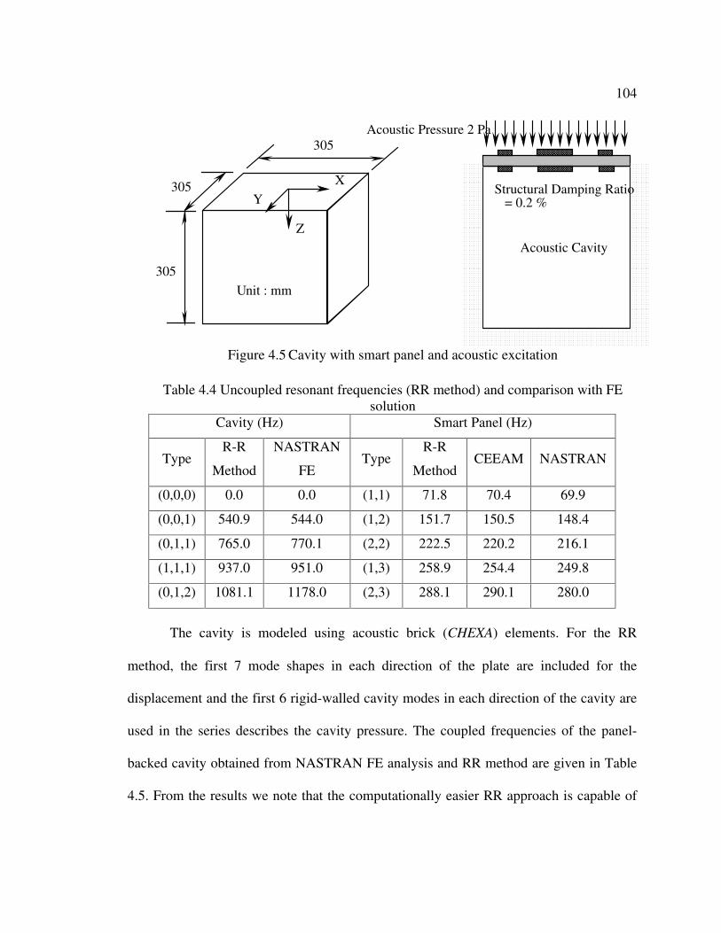
104
Table 4.4 Uncoupled resonant frequencies (RR method) and comparison with FE solution
Cavity (Hz) Smart Panel (Hz)
Type R-R
Method
NASTRAN
FE Type
R-R
Method CEEAM NASTRAN
(0,0,0) 0.0 0.0 (1,1) 71.8 70.4 69.9
(0,0,1) 540.9 544.0 (1,2) 151.7 150.5 148.4
(0,1,1) 765.0 770.1 (2,2) 222.5 220.2 216.1
(1,1,1) 937.0 951.0 (1,3) 258.9 254.4 249.8
(0,1,2) 1081.1 1178.0 (2,3) 288.1 290.1 280.0
The cavity is modeled using acoustic brick (CHEXA) elements. For the RR
method, the first 7 mode shapes in each direction of the plate are included for the
displacement and the first 6 rigid-walled cavity modes in each direction of the cavity are
used in the series describes the cavity pressure. The coupled frequencies of the panel-
backed cavity obtained from NASTRAN FE analysis and RR method are given in Table
4.5. From the results we note that the computationally easier RR approach is capable of
Acoustic Cavity
X
Y
Z
305
305
305
Unit : mm
Structural Damping Ratio = 0.2 %
Acoustic Pressure 2 Pa
Figure 4.5 Cavity with smart panel and acoustic excitation

105
predicting the dynamics of the smart panel-cavity system accurately when compared with
the FE results.
Table 4.5 Coupled frequencies of the smart panel-cavity R-R Method
(Hz)
NASTRAN/FE
(Hz)
Experiment
(Hz)
0.0 0.0 -
84.5 85.3 85.7
155.7 151.9 -
252.8 249.8 256.0
315.4 304.3 -
The size of the system matrices resulting from the RR method for the present case is
265×265 and the FE system matrices have size of 800×800. This difference will
considerably increase for higher frequencies. For noise control studies, a uniform
harmonic pressure load of 2.0 Pa, which excites the panel at its first two resonant
frequencies, is applied on the panel surface. The pressure at the center of the cavity
2
,2
,2
zyx lll is computed with and without velocity feedback control and is given in
Table. 4.6
Table 4.6 Transmitted noise inside the cavity (RR method) Pressure at the center of the
Cavity (dB) Excitation
Frequency
(Hz) Without
Feedback
With velocity
Feedback
84.5 108 94
252.8 92 73

106
A simple velocity feedback control law sa gain VIV ××−= is used in which gain
is the feedback gain value and I (5×5) is an identity matrix. From Table 4.6, we observe
that the velocity feedback control using discrete sensor/actuator patches reduces the
transmitted pressure by 14 dB for the first mode excitation and by 19 dB for the second
mode excitation. We also see from equation (4.33), that the voltages induced in the
sensors and the actuation forces supplied by the actuators are multiplied by the term
dydxyx
TT
∫ ∫
∂∂+
∂∂
22
FF, which is a function of the displacement of the plate. This
particular function, hereafter called amplification function, is plotted over the area of the
plate in Fig.4.6 to Fig. 4.9 for the first four resonant modes of the plate. From the figures
we observe that the peak values of the amplification function for any specific mode
indicates the optimal positions of the sensors and actuators for controlling that particular
mode. The long white dash dot lines represent the nodal lines (zero magnitude lines);
over which if the sensor/actuators were placed would become ineffective. These
amplification functions mapped, using either the mode shapes or the total response, can
be used for rectangular plates to identify the optimal positions of the actuators and
sensors.

107
Figure 4.7 Amplification function for mode 2
Figure 4.6 Amplification function for mode 1

108
Figure 4.8 Amplification function for mode 3
Figure 4.9 Amplification function for mode 4
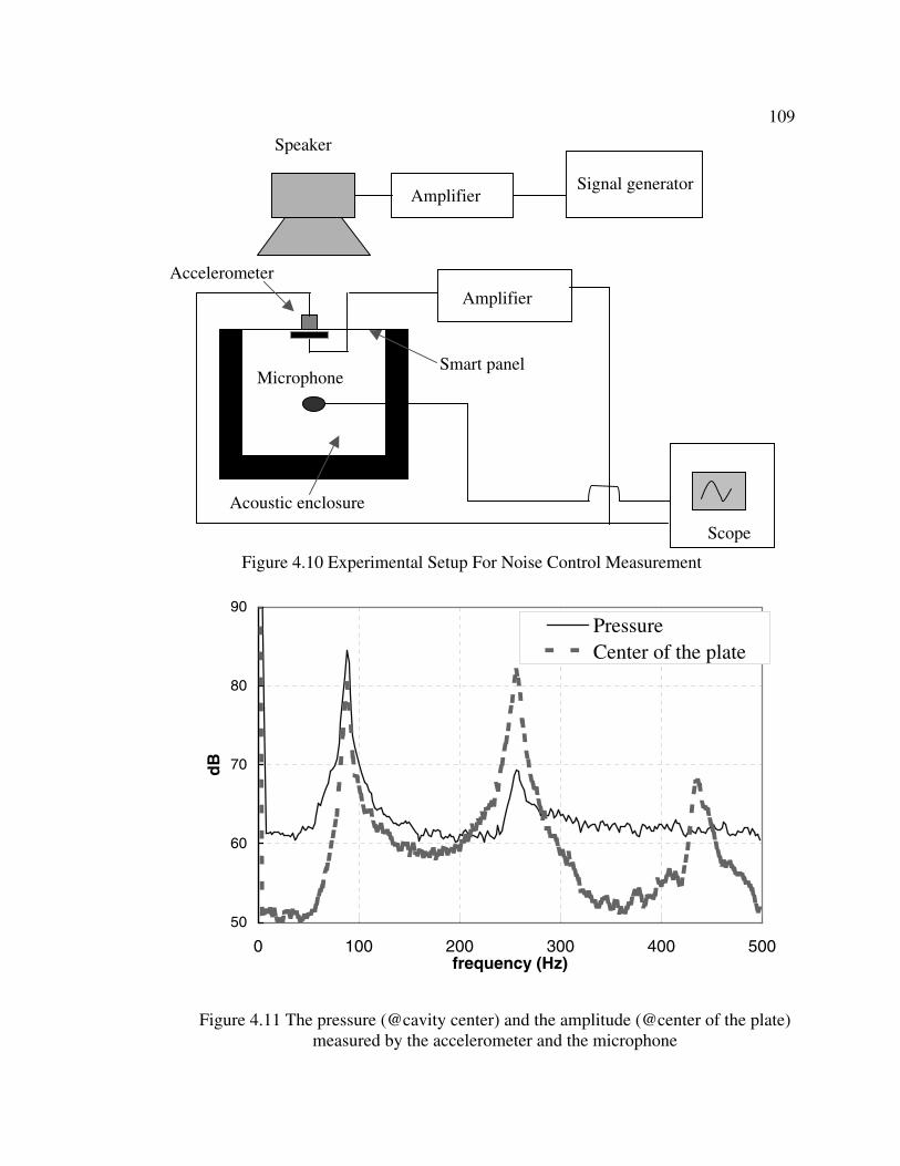
109
50
60
70
80
90
0 100 200 300 400 500frequency (Hz)
dB
PressureCenter of the plate
Figure 4.11 The pressure (@cavity center) and the amplitude (@center of the plate) measured by the accelerometer and the microphone
Figure 4.10 Experimental Setup For Noise Control Measurement
Accelerometer
Amplifier Signal generator
Smart panel
Speaker
Amplifier
Acoustic enclosure
Scope
Microphone

110
Figure 4.10 shows the schematic diagram of the experimental setup used to
determine the resonant frequencies for validating the RR model. The accelerometer
senses the vibration levels at the center of the panel and a microphone inside the cabin
senses the sound pressure levels. A B&K signal generator generates a chirp signal with a
frequency range of 40 Hz to 500 Hz. This signal is then fed to a speaker, which generates
a pressure field on the top surface of the smart panel thus simulating an external
disturbance for the cavity-panel system. Figure 4.11 shows the frequency response of the
accelerometer bonded at the center of the plate and the microphone placed at the center of
the cavity. From the plot we observe that the responses are maximum at the resonant
frequencies of the coupled system, which are shown in Table 4.5. The accelerometer and
the microphone sensed only the symmetric modes because of the nature of the noise
loading and their position on the plate and inside the cavity.
4.10 Summary
The analytical model for a smart plate bonded with discrete piezoelectric patches
is developed without any assumptions on the strains inside the patches. The classical
plate theory and the electroelastic theory are used in deriving the dynamic equations of
motion for the smart plate. Though the examples used here includes only one pair of
collocated sensor/actuator patches the solution can be obtained for any number of
sensor/actuator pairs bonded to the host plate. The effect of the passive stiffnesses on the
dynamic behavior of a host isotropic plate structure is studied. We observed that the
presence of the patch changes the natural frequency considerably for of a smart plate with

111
surface bonded PZT piezoelectric patches. So the effects of passive stiffness cannot be
neglected particularly for the Micro Electro Mechanical Systems (MEMS) applications
where precise estimation of the frequencies is mandatory. For such applications the
present analytical model can be used to estimate the dynamic characteristics of the smart
plate. The effect of active stiffness and damping provided by the patch due to a closed
loop system using the present modeling approach is presently difficult to obtain and
should be attempted in the future. Alternatively, the Rayleigh-Ritz method is developed
for modeling the plates with surface bonded discrete type actuators and sensors and
extended for an active noise control system using this smart panel. A smart aluminum
plate backed cavity is studied using this method and the results are compared with FE
analysis and experimental results. From the results we conclude that the RR approach is
quite accurate in predicting the dynamic behavior of the vibroacoustic system with an
active noise control system. Results of studies showed that the RR model, which can
predict the first few frequencies at the same level of accuracy, could execute four times
faster than the corresponding FE model. At high frequencies, the FE method requires
larger matrices, which are computationally expensive. Controller design and optimal
placement of actuator/sensor pairs using the RR approach is preferred over the FE
method due its simplicity and smaller computational size. For problems involving
irregular boundaries and complicated boundary conditions, it is not possible to define a
global shape function. In such cases, the RR approach loses some of its advantages over
the FE method. Though the method developed here is used to study an isotropic panel,
the approach is applicable to a general orthotropic smart panel-cavity system.

112
CHAPTER 5
FINITE ELEMENT SIMULATION OF SMART PANELS FOR
VIBRATION AND NOISE CONTROL APPLICATIONS
5.1 Introduction
The design of efficient structural systems is of fundamental interest to
both structural and control engineers. Systematic methodologies for both structural and
active control system syntheses are well known and are receiving increased application in
the design environment. Control system design for large flexible structures is an
important and difficult problem because of the interaction between a structure and a
control system in active vibration control. A number of important practical considerations
such as the discretization of continuum models, total number of actuators and sensors
used and their placement, and controller design must be taken into account before real
implementation of active control can be put into action. The modeling and analysis of
adaptive piezoelectric structures represents a high level of sophistication and complexity.
Thus, the development of admissible mechanics for the numerical model as well as a
sophisticated control algorithm for smart structures poses a great challenge. For given
piezoelectric materials, structure, and control domain, an optimum procedure should be
investigated for controlling the vibrations of the system.
There are two major experimental approaches to structural vibration control. One

113
uses distributed sensors and actuators in the form of piezoelectric polymer films (PVDF)
that cover the entire structure and the electrodes deposited on these films are often shaped
to shape the electric field to achieve the desired control. These sensors and actuators are
called mode shape sensors and actuators because they respond and control only particular
modes of vibration. The difficulty with this approach is that it is impractical and
expensive to cover the whole structure or a large part of the structure with piezoelectric
films. This changes the structural response of the system completely and there are major
manufacturing difficulties. The optimal size, thickness and location of a single
piezoelectric actuator on a flat plate for reducing the radiated sound are studied by Kim et
al (1995), who have observed that for an optimal configuration of the patch type actuator,
the voltage requirement is low.
Like the previous one this chapter also focuses on piezoelectric actuator
and sensor patches that occupy a relatively small area of structures. It is unreasonable to
use one sensor to obtain the vibration information of all points of the structure. Also, it is
difficult to use one single actuator to control the vibration of structure. Most structures
need multiple sensors and actuators to accurately observe and to effectively control the
fundamental modes that dominate the structural vibration. The system thus becomes a
multi-input-multi-output (MIMO) structure. Piezoelectric transducers made of PZT are
also relatively thicker and smaller in size compared to the structure and are spatially
distributed in many practical applications. Therefore, discrete sensors and actuators are
preferred over distributed piezoelectric films for the multimode control of structures.
The fundamental problem of actively controlling flexible systems is to control a

114
very large dimensional system with a much smaller dimensional controller. The selection
of appropriate feedback gains thus presents the difficulties for large-scale structures that
require an infinite number of vibration modes to describe their dynamic behavior.
Moreover, because of economical reasons and the limitations of on-board computer
capability, the number of sensors and actuators available are restricted. To overcome
these difficulties, output feedback controllers are preferred. An output feedback system
applies control gains directly to sensor outputs, and these signals are fed back to the
control actuators. Thus, this method is favorable for the application of discrete
piezoelectric sensors and actuators to control the large-scale structures. This control
hierarchy provides many advantages over the existing state feedback control. No state
estimator is involved in this approach and, consequently, this greatly simplifies the
internal complexity of the controller and reduces the on-board computer requirement.
Since large-scale structures involve a large number of degrees of freedom, modal
reduction techniques are normally used to reduce the system model for controller designs
instead of physical coordinates. This can be achieved by eigenvector assignment using
output feedback control. Consequently, active control is reduced to a few low
fundamental modes in control of structures in which the high frequency residual modes
are truncated. The optimal control simulation of piezoelectric smart structures has been
successfully investigated in modal space by using the finite element method (Rao and
Sunar 1993, Chen et al 1997). Many earlier researchers adopted the state feedback
control and assume a perfect knowledge about the space, even though the state has to be
reconstructed from the sensor signals by the observer in the actual situation. In most

115
applications, particularly in those involving flexible large structures, the plate state
(modal coordinates) cannot be physically measured or resolved without employing
elaborate and model dependent state estimators. Under these conditions, the
implementation of the control algorithm may encounter significant difficulties. Also, this
approach cannot provide a natural and logical mechanism for implementing the discrete
multiple-input-multiple-output control methodologies.
To overcome the drawbacks of state feedback, the optimal control objective to be
achieved by modal output feedback computes the gain matrix to increase the modal
damping ratios and natural frequencies of the selected fundamental vibration modes.
However, it is not always possible to design the controller to be as stable as necessary
since structural vibration reduction is not always guaranteed. This limitation usually
comes when the number of sensors and actuators are a lot smaller than the number of
vibration modes to be controlled. If there are enough pairs of sensors and actuators, then
the output feedback control will show performance similar to state feedback control. The
optimal output feedback problem is thus a significant extension of the optimal full state
feedback problem.
In this chapter, five collocated sensors and actuators are used to effectively
control ten modes of the flexible smart panel at different locations. It is well known that
collocated sensors and actuators are advantageous from the viewpoint of stability. Also,
controllability and observability matrices are full rank, so it is possible to assign virtually
arbitrary stability to the controller. This present work demonstrates a detail description of
the integrated finite element capability using output feedback for a controller based on

116
Linear Quadratic optimal control. For a numerical example, a hybrid approach using a
finite element formulation for the radiating walls of an enclosure is also presented.
Interior noise control in a cabin enclosure using active vibration control of the walls of
the enclosure with discrete modeling technique is demonstrated. Though the control
forces depend only on the state of the system, namely displacement and velocity, the
reduction in the sound pressure level is achieved through actively controlling the modes
of vibration, which contribute to the radiated pressure inside the enclosure.
5.2 Formulation
The finite element formulation of the structure is considered first. The modeling
approach for the acoustic cavity is shown in subsequent sections. Finally the coupling of
both models and the design of an optimal controller are discussed.
5.2.1 Finite Element Model Of The Panel Structure
The variational principle can be used to derive the finite element equations for
coupled electro-elastic continuum. The approach used here to derive the dynamic
equations of motion is based on the work carried out by Allik and Hughes (1970). The
linear constitutive equations relating the elastic field and electric field can be written as
,
,
EbhSD
EhSCTs
TE
+=−=
(5.1)
where
T = Stress Tensor, D = Electric Displacement,
S = Strain tensor, h = Piezoelectric coupling coefficient,

117
E = Electric Field, bs = Dielectric constant at constant strain, and
CE = Elastic stiffness tensor evaluated at constant E field.
Dynamic equations of a piezoelectric continuum can be derived using Hamilton’s
principle,
02
1
=∫ dtt
t
Lδ , (5.2)
where the operator δ denotes the first order variation and t1 and t2 define the time interval,
and all variations must vanish at t = t1 and t = t2. The Lagrangian L is determined by the
energies available in the piezoelectric medium:
WEEL skin +−= , (5.3)
where the kinetic energy Ekin is given by VuE dkin ∫= 2
2
1ρ and the elastic and dielectric
energy ( ) VDETSE TT dS 2
1∫ −= . Here ρ is the mass density and u is the velocity vector
and V is the volume of the piezoelectric medium. The energy W stored in the medium
due to the external mechanical and electrical excitation is defined as
∫ ∑∫ ∫ ∑ +−++=21
2
s
cs
V s
cT
sT
bT qdSqfudSfdfW φφuVu , (5.4)
where fb is the body force, fs is the surface force, fc is the concentrated force and qs is the
surface charge, qc is the point charge and S1 is the area where mechanical forces are
applied and S2 is the area where electrical charges are applied.

118
Substituting the equations (5.3) and (5.4) into equation (5.2) and taking the first
variation on L, and integrating by parts, we get
. 0
21
21
=+−+−
−+−−−
∫∫
∫
ccT
s
s
s
sT
bTT
V
qfdqdf
df
δφδδφδ
δρδδδδδ
uSSu
VuuuEbEhSEEhSSCS STTTTET
(5.5)
Now the electroelastic continuum is discretized with finite elements and the
displacement u and the electric potential φ are expressed in terms of nodal values via
interpolation functions
,
,
i
iuu
Φ==
φφ N
Nu (5.6)
where Nu and Nφ are the interpolation functions for the field variables for u and φ and ui
and φi are the nodal point values.
fs S1
S2
qs fc qc
S
V
Figure 5.1 An elastic continuum with piezoelectric elements and external forces

119
It is to be noted that the linear shape functions for φ are identical to those for the
displacement vector u. The shape functions Nφ and their derivatives are defined for the
conventional isoparametric element.
The mechanical strains S are related to the nodal displacements through the
derivative of the shape function Bu
iuuBS = , (5.7)
where Bu is the strain-displacement matrix. Similarly the electric field E is related to the
nodal potential by
iΦ−=−∇=∇= φφφφ BNE , (5.8)
where Bφ is the electric field-displacement matrix.
Substituting equations (5.6)-(5.8) into equation (5.5) results in, for all values of
virtual displacements, the two equilibrium equations:
[ ] [ ] [ ] [ ] [ ] ,
and ,
QKuK
FKuKuM
=Φ+
=Φ++
φφφ
φφ
Tu
uuuu (5.9)
where
[ ] dVuTuuu NNM ∫= ρ is the mass matrix,
[ ] dVu
T
uuu BCBK ∫= is the elastic stiffness matrix,
[ ] dVTT
uu φφ BhBK ∫= is the piezoelectric coupling matrix,
[ ] dVsT
φϕφφ BbBK ∫−= is the dielectric stiffness matrix,

120
cTu
S
sTs
V
bTb fdSfdVf NNNF ++= ∫∫ 1
1
1 is the mechanical force, and
cT
s
S
Ts dSq qNNQ φ−−= ∫ 22
2
2 is the electrical charge.
The above matrix equations are written in partitioned form to reflect coupling
between the elastic and electric fields. The structural linear viscous damping term
uC ][ uu can be added in the first matrix equation (5.9) where [ ] [ ] [ ]uuuu KMC λη += uu is
the system damping matrix in which η and λ are called Rayleigh coefficients.
The electric field boundary condition requires that the electrode surface is an
equipotential one and the summation of the nodal electric charges on it should be zero on
the sensor electrodes since they are in ‘open circuit’ conditions:
Constant...1 ==Φ=Φ +ii and ( ) 0=∑ sensoriQ . (5.10)
5.2.2 Condensation of System Matrices
The external charge applied on the actuator surface needs to be properly provided
to produce the desired control forces. The external charge applied on the actuator surface
needs to be properly modeled and cannot be neglected in order to produce the desired
control forces. Equation (5.9) can be condensed to write the sensor potential in terms of
the sensor displacement as
[ ] [ ] uKK
u
−
=
− Tu
I
φφφφ 1 . (5.11)
After assembling all element matrices, and substituting the foregoing
transformation matrix into eqn. (5.9), the system dynamic equation is written as

121
[ ] [ ] cacextuu FFFuKuM ++=+ * , (5.12)
Where
[ ] [ ] [ ][ ] [ ] [ ][ ] .
and , 1
1*
QKKF
KKKKK−
−
=
−=
φφφ
φφφφ
uc
Tuuuu
extF and cF are the external mechanical force acting on the structure and the
electrical force, respectively. The electric force is contributed directly by the external
applied electric charge Q . Ha (1992) considers that the voltage is the only form of
electrical input to the actuator. He did not consider the effect of charge. However,
external electric charge will play a very important role in vibration control applications.
The force vector acF is due to the pressure loads acting on the structure when the
structure is in contact with the fluid in the cavity.
The electrical potential can be recovered from
[ ] [ ][ ]uKQK 1 T
uφφφ −=Φ −. (5.13)
Note that Q is zero in the sensor. Thus, the sensor equation is
[ ] [ ]( )uKK 1 T
us φφφ −=Φ −. (5.14)
5.3 Control Mechanism
The sensor generates voltage outputs when the structure is oscillating. The signal
can be amplified and fed back into the actuator using an appropriate controller. The
feedback signal to the actuator is represented as
svsda Φ+Φ=Φ GG , (5.15)

122
where the subscript a is for the actuator and s is for the sensor. The quantities sΦ and
sΦ are obtained from the sensor equation (5.14). Gd and Gv represent respectively the
displacement feedback control gain and the velocity feedback gain. As the gains are
constant with respect to time and frequency, this controller is known as a constant gain
feedback controller. The direct effect in the piezoelectric actuator is negligible because
the feedback voltage is much higher than the self-generated voltage.
5.3.1 Direct Charge Approach
When piezoelectric materials are used for actuation, an electric charge Q is
usually applied to the distributed piezoelectric actuator, and this charge is responsible for
the potential difference that appears between two electrodes of the actuator. The electrical
charge Q and electric potential can be related by
[ ] aCQ = , (5.16)
where [C] is the capacitance of the piezoelectric actuator, and a is an external voltage
applied on the piezoelectric actuator. The voltage output resulting from the distributed
sensors is amplified and fedback into the distributed actuators as feedback voltages. Thus
multiplying equation (5.15) by the capacitance of the actuator, one can derive the
feedback charge injected into the actuator as
( )svsd GGC Φ+Φ= Q . (5.16)
The piezoelectric capacitance of the actuator modeled as a parallel plate capacitor
can be defined as pzttC /33Aε= , where ∈33 is the z-directional permittivity of

123
piezoceramics, A is the actuator area and tpzt is the actuator thickness.
Substituting the feedback charge into equation (5.9) and utilizing the sensor
output signal, the feedback force can be reformulated in matrix form as follows:
[ ][ ] [ ][ ] [ ] [ ][ ] [ ][ ] [ ][ ] [ ] ,
1111
uCuK
uKKGKKuKKGKKF
ctrlctrl
Tuvu
Tuduc
−=
−−= −−−−φφφφφφφφφφφφ (5.17)
where [ ] [ ][ ] [ ][ ] [ ]φφφφφφ
Tuvuctrl KKGKKC 11 −−= is the active damping matrix for charge
control and [ ] [ ][ ] [ ][ ] [ ]Tuductrl φφφφφφ KKGKKK 11 −−= is the active stiffness matrix for charge
control, [ ]dG and [ ]vG are the displacement feedback gain matrix and the velocity
feedback matrix, respectively. [ ]ijd ,G and [ ]ijv ,G
have the meaning that sensed voltage of
the jth piezoelectric element is fed back to control the ith piezoelectric element. The
feedback control forces should be applied to piezoelectric actuators depending upon the
information of velocity and displacement gain components.
Substituting this feedback force into the system equation (5.15) gives the
governing equation of motion as
[ ] [ ] [ ][ ] [ ][ ] [ ] [ ] [ ][ ] [ ][ ] [ ] . 11*
11
FuKKGKKK
uKKGKKCuM
=++
++−−
−−
Tudu
Tuvuuuuu
φφφφφφ
φφφφφφ
(5.18)
5.3.2 Direct Voltage Approach
If voltage is applied directly on the electrodes of the actuators then in equation
(5.15) we substitute directly the voltage magnified by gain into the actuator voltage a
degrees of freedom, equation (5.9) can be rewritten as

124
[ ] [ ]
=
ΦΦ+Φ=Φ
++
0
Q
Fu
KK
KKuCuM
s
svsdaTu
uuuuuuu GG
φφφ
φ , (5.19)
where the electrical potential vector Φ can be divided into two groups, a the
potential vector at the actuator nodes and s the potential vector at the sensor nodes. Q
contains the unknown nodal forces related to the actuator electrical potential, which may
be derived from sensor equation (5.14). Therefore, charge can be found later after
substitution of unknown degrees of freedom, and we can directly solve the above
equation.
5.4 Eigenvalue Analysis
Before solving the equation of motion of a structure with the piezoelectric
devices, the mode shapes and the resonant frequencies of the undamped system are
obtained using Eigenvalue analysis. Solution of the Eigenvalue problems may use the full
assembled matrices or the reduced matrix system obtained by matrix condensation of
structural and potential degrees of freedom. Free vibration implies that
0 and 0 == QF in equation (5.9). Unspecified potentials are then condensed out of the
matrices reducing the equations (5.9) to
[ ] [ ] 0UMK* =− uu2ω , (5.20)
where ω is the natural frequency. The new stiffness matrix [K*] indicates that the
structure is electromechanically stiffened.

125
5.4.1 Modal Analysis
The system equation of motion shown in equation (5.18) is not suitable for
system analysis because the order of degrees of freedom of the system u is usually too
large in finite element method. Therefore, the equation has to be transformed into a set of
properly chosen modal coordinates with much smaller and manageable degrees of
freedom to supply great computer efficiency. The modal analysis is based on the
orthogonality of natural modes and expansion theorem.
The modal extended displacement u is represented by
[ ]qU=u , (5.21)
where [U] is the modal matrix, and q are referred to as modal coordinates.
The modal matrix [U] is simply a square matrix in which the columns
corresponding to eigenvectors of the system, satisfying an eigenvalue problem shown in
equation (5.20). Substituting equation (5.21) into equation (5.18) and multiplying two
sides of equation (5.18) by [UT] gives
[ ][ ][ ] [ ][ ][ ] [ ][ ][ ] [ ][ ][ ] [ ] FUUKUUKUUCUUMU Tctrl
TTctrl
Tuu
T qqqq =+++ * (5.22)
Considering the orthogonality property, the above equation can be written as
[ ] [ ][ ][ ] [ ] [ ][ ][ ]( ) [ ] FUUKUIUCUI Tctrl
Tctrl
T qqq =+−++ 2ω
(5.23)
Equation (5.23) is recognized as a closed-loop equation of motion. The process of
using the above equation to control the system is known as modal control. Note that the
rate feedback modifies the damping matrix of the system, and the displacement feedback
modifies the stiffness matrix of the system. Before the behavior of the closed-loop system

126
can be established, it is necessary to determine the control gain.
5.5 Output Feedback Optimal Control
The Linear Quadratic Regulator (LQR) controller based on the modal space
model is proposed and the explicit solutions are used for the corresponding Riccati
equations of the output feedback optimal controller. In the most general case some of the
piezoelectric patches act as actuators and others as sensors, and it is therefore necessary
to partition the electrical potential Φ to extract actuator and sensor contributions. By
using transformation matrices Ta and Ts respectively, for the vectors of the voltages at the
actuators and at the sensors, the equation of motion (5.23) and the sensor output equation
(5.14) in terms of a modal coordinate can be expressed as
[ ] [ ] [ ] [ ] [ ] [ ][ ] [ ][ ][ ] [ ][ ]q,UKKT
TKKUFUqqqT
φφφ
φφφωςω
u1
1u
2 and , =2+−
−
−=Φ
Φ−+
ss
aaTTI
(5.24)
Ta is an m× n actuator location matrix for the actuator degrees of freedom and Ts is an
n×m sensor location matrix for the sensor degrees of freedom
Here m is the number of total electrical potential degrees of freedom and n is the
number of sensors and actuators. The columns of Ta matrix respectively consist of the
piezoelectric capacitance values of actuators corresponding to the actuator degrees of
freedom, where the rows of the Ts matrix contain unit values at the sensor degrees of
freedom. The control forces are provided by n number of actuators and the sensor
voltages are also measured by n number of sensors.
The governing equations can be written in modal state space form to provide a

127
standard mathematical basis for control studies. The linear time-invariant equations of
motion which include the effects of piezoelectric control forces and external disturbance
force are expressed as follows
FBB+xA=x da +Φ
aq
q=
, xC=Φ s , (5.25)
where
[ ] [ ]
−=
ζωω 2
2
IA
0,
[ ] [ ][ ] [ ]
− −a
T TKKU
Ba 1
u φφφ
0= ,
[ ][ ] [ ][ ][ ]UKKTC Tφφφ u
10 −−= s , and [ ]
TU
Bd
0= ,
where A, Bd, Bu and C are the corresponding state, disturbance, control and sensor
matrices. The transfer functions matrices in terms of these state-space matrices are
.)()(
and ,)()(1
1
dd
aa
ss
ss
BAICP
BAICP−
−
−=
−= (5.26)
In direct output feedback, control forces are calculated directly from the
multiplication of output measurements by constant feedback gains, expressed as
( )svsd GGC Φ+Φ= Q , (5.27)
where G is the time-invariant output feedback gain matrix to be determined by the design
procedure. Control forces are just some combinations of output measurements, which in
turn are combinations of system states. Based on this representation, the optimal
controller can be formulated by calculating the applied voltage to minimize a linear
quadratic performance.

128
dtJ aTa
T )(0
RQxx∫∞
+= , (5.28)
where Q (positive semi definite) and R (positive definite) are weighting matrices to be
selected by the designer. The optimal solution is found from the procedure of (Levine and
Athans 1970) that minimizes the expected value of performance index
)(tr PX=J where )0()0( TE xxX = , (5.29)
where P satisfies the Ricatti equation
0TTT =+++ QRGCGCPAPA cc . (5.30)
By applying optimality conditions for the above problem, the optimal control gain
matrix G can be obtained by solving the following coupled nonlinear algebraic matrix
equations simultaneously with equation (5.30):
0XSASA Tcc =++ , and (5.31)
1TTT1 )(CSCPSCBRG −−= . (5.32)
Note that P, S and G are matrices to be determined from the above three equations. Ac
denotes the closed loop system matrix
BGCAAc −= . (5.33)
There exist several numerical approaches to solving equations (5.30-5.32). In this
study, the effective iterative solution algorithm proposed by Moerder and Calise (1985) is
adopted. The weighting matrix Q for the modal space quadratic performance index is
usually assumed to be diagonal and takes the form (Meirovitch et al 1983)
)1...1...(diag 221 nωω=Q . (5.34)

129
However, there are no general guidelines for the choice of R , the weighting matrix for
control forces. A diagonal R , as assumed in most applications, may be written as
)...(diag 21 nrrr=R . (5.35)
5.6 Radiated Sound Field Inside a Rectangular Enclosure
Although there are many possible theoretical models for the enclosed sound
fields, the modal model, which is more appropriate for low frequency applications, is
used here. In the low frequency range the modal model of an enclosed sound field
requires relatively few parameters for an adequate description of the spatial and
frequency dependency of the field. In this model the pressure at any point inside the
enclosure is expressed as the sum of acoustic mode shapes of the cavity. These mode
shapes correspond to the eigenfunctions of the homogenous Helmholtz equation with the
rigid wall boundary condition.
The modal representation of the acoustic pressure can be written as
))cos()cos()(cos(c
zn
b
yl
a
xlAAp lmnlmnlmn
πππΣ=ΨΣ= , (5.36)
where Almn are the unknown modal weighting coefficients and l, m, n are the cavity mode
numbers.
The inhomogeneous Helmholtz equation for the cavity pressure field, generated
due to the vibration of walls is given as
nupc
p 202
22 ωρω =
+∇ , (5.37)
where un is the normal structural displacement and can be written in terms of the shape

130
functions (Ns) and the nodal displacements (us) of the structural finite element as
ssnu uN= . (5.38)
Substituting the assumed pressure field in equation (5.37) and using the
orthogonality property of the modes, we find modal weights Almn as
lmn
lmnss
lmn
c
n
b
m
a
l
c
dsuN
A
Λ
+
+
−
−=
∫2222
02 )(
πππω
ψρωS , (5.39)
where dxdydzc
zn
b
ym
a
xla b c
lmn )(cos)(cos)(cos 22
0 0 0
2 πππ∫ ∫ ∫=Λ .
The force exerted on the plate structure by the pressure field inside the cavity is
calculated as
ss slmnlmns sfluid udsNAdspNF ∫∑∫ −=== H2ωψ , (5.40)
where
( )dSN
c
n
b
m
a
l
c
dsN
slmnS
lmn
S
lmns
Ψ
Λ
+
+
−
Ψ−=∑∫
∫2222
0
πππω
ρH .
The finite element equation of motion for the smart plate structure is rewritten by
including this force term along with the other external forces acting on the plate structure.
The final coupled fluid-structure finite element equation of motion is written as
[ ] [ ] [ ][ ] FUKKCHM =+++−− ctrlctrluu i *2 ωω . (5.41)
The above equation can be solved for the displacements and weighting
coefficients Almn, from which the pressure at any point inside the cavity can be

131
determined from the equation (5.37).
5.7 Numerical Simulations of the Clamped Plate
To utilize the advantages of piezoelectric transducers, it is necessary to select
appropriate positions of the transducers and to select the sensor signals that are to be fed
back to the actuators. The problem of selecting the locations of transducers is a complete
problem in itself. In this research, the actuator/sensor pairs are pre selected and held at a
fixed location during an optimization search for control gain. The modal order and the
corresponding mode shape function provide a significant insight of the best actuator
locations on vibration control. Effective sensing and control depend on the locations of
sensors and actuators. The actuator locations are studied in order to maximize actuator
effectiveness. The positions of the plate at which the mechanical strain is highest are the
best locations for sensors and actuators. Therefore, the objective of the multimode control
is to place all of the actuators in regions of high average strain and away from areas of
zero strain (anti-nodal line). One advantage of using this prediction guarantees the fewest
number of sensors and actuators, the least power and the least coverage of structural area.
This method is derived from a structural mechanics standpoint and is relatively simple.
The analysis of active vibration control is performed for the clamped plate. The size of
the aluminum plate is 0.305m × 0.305m and the thickness is 0.8 mm. The five
piezoelectric patches made of PZT-5H are used as collocated sensors and actuators over

132
Transition element
3-D Solid elements
Shell element
(a) 20 node solid element (b) 13 node transition element (c) 9 node shell element
A91.25
76.25
Unit : mm
Case I
Harmonic force excitation :
t (sec)
F (N)
-0.1
Unit step excitation :
79.5
67.92
142.3
125.5
111.6
58.5
43.9
43.9
C
D
F
E
Unit : mm
Harmonic force excitation for arbitray points:
Fc= -0.1 sin(50t) Fd= 0.3 cos(40t) Fe= 0.5 sin(60t)
: Control Activate
Case II
F = 0.1 e− iω t N
Figure 5.2 Aluminum panel with five surface bonded collocated piezoelectric actuators/sensors and schematic diagram of two loading cases
Figure 5.3 Modeling of a geometrical transition with several types of finite element.

133
the upper and lower surfaces for multimode control of vibration of the plates (Fig. 5.2).
Figure 5.3 and 5.4 show the elements used and the finite element mesh for the smart
plate.
Twenty-four 20-node solid elements are used for modeling the solid piezoelectric
patches and the part of the plate beneath the piezoelectric patch. Around the piezoelectric
patch, twenty-four 13-node transition elements are used to connect the solid elements to
the remaining part of the plate that is modeled by 9 node flat-shell elements. A total of
136 nine node flat-shell elements are used to model the plate. The upper piezoelectric
elements are used as actuators and the lower ones as sensors. The first 10 modes of the
proposed finite element model are calculated using eigenvalue analysis. The mode shapes
upon activation of the embedded collocated piezoelectric patches for the pure plate are
shown in Fig. 5.5.
From previous chapters we found that the center of the plate is an appropriate
Figure 5.4 Finite element model with piezoelectric sensors and actuators
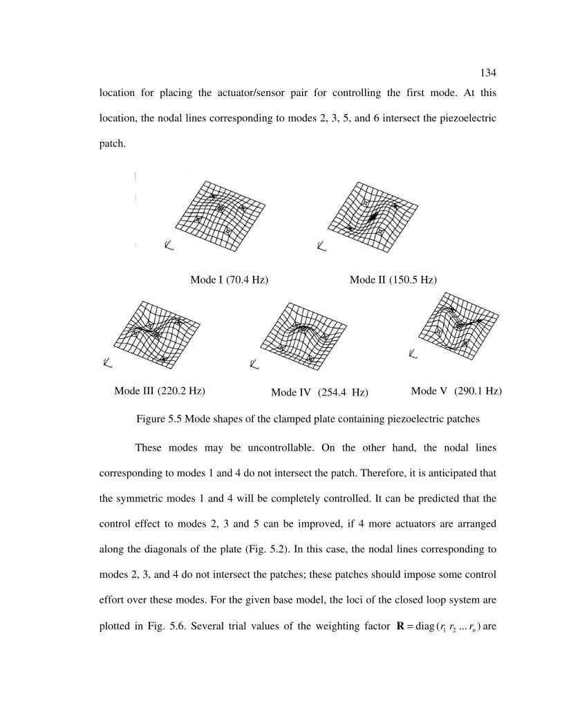
134
location for placing the actuator/sensor pair for controlling the first mode. At this
location, the nodal lines corresponding to modes 2, 3, 5, and 6 intersect the piezoelectric
patch.
These modes may be uncontrollable. On the other hand, the nodal lines
corresponding to modes 1 and 4 do not intersect the patch. Therefore, it is anticipated that
the symmetric modes 1 and 4 will be completely controlled. It can be predicted that the
control effect to modes 2, 3 and 5 can be improved, if 4 more actuators are arranged
along the diagonals of the plate (Fig. 5.2). In this case, the nodal lines corresponding to
modes 2, 3, and 4 do not intersect the patches; these patches should impose some control
effort over these modes. For the given base model, the loci of the closed loop system are
plotted in Fig. 5.6. Several trial values of the weighting factor )...(diag 21 nrrr=R are
Mode I(70.4 Hz) Mode II(150.5 Hz)
Mode III(220.2 Hz) Mode IV (254.4 Hz) Mode V (290.1 Hz)
Figure 5.5 Mode shapes of the clamped plate containing piezoelectric patches
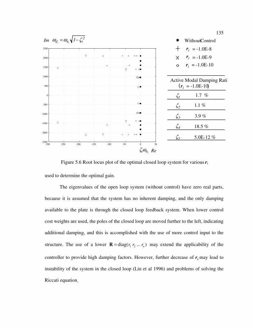
135
used to determine the optimal gain.
The eigenvalues of the open loop system (without control) have zero real parts,
because it is assumed that the system has no inherent damping, and the only damping
available to the plate is through the closed loop feedback system. When lower control
cost weights are used, the poles of the closed loop are moved further to the left, indicating
additional damping, and this is accomplished with the use of more control input to the
structure. The use of a lower )...diag( 21 nrrr=R may extend the applicability of the
controller to provide high damping factors. However, further decrease of rI may lead to
instability of the system in the closed loop (Lin et al 1996) and problems of solving the
Riccati equation.
-300 -250 -200 -150 -100 -50 0 50-2500
-2000
-1500
-1000
-500
0
500
1000
1500
2000
2500
Without Control
= -1.0E-8
= -1.0E-9
= -1.0E-10
Re
Im
Active Modal Damping Rati
1.7 %
1.1 %
3.9 %
18.5 %
5.0E-12 %
ωdi=ωni
1−ζi2
ζiωni
ri
ri
ri
ζ1
ζ2
ζ3
ζ4
ζ5
= -1.0E-10ri( )
Figure 5.6 Root locus plot of the optimal closed loop system for various ri
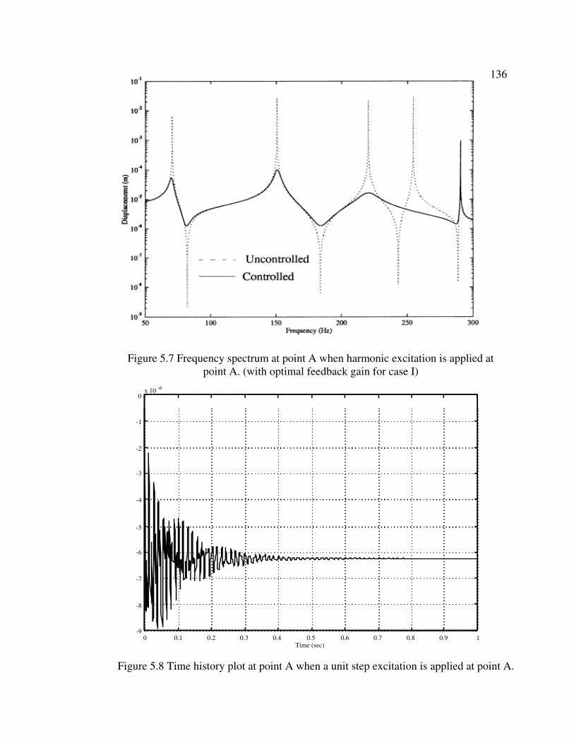
136
Figure 5.7 Frequency spectrum at point A when harmonic excitation is applied at point A. (with optimal feedback gain for case I)
0 0.1 0.2 0.3 0.4 0.5 0.6 0.7 0.8 0.9 1 -9
-8
-7
-6
-5
-4
-3
-2
-1
0 x 10 -6
Time (sec)
Figure 5.8 Time history plot at point A when a unit step excitation is applied at point A.

137
The weighting value for the optimal control is therefore chosen to be 10100.1 −× .
All structural modes are not controlled in applying the output feedback optimal control.
The control input is directed to modes that dominate the response. The active damping
values for the closed loop system are also listed in Figure 5.6. The first four modes are
significantly damped. However, for the fifth mode, the damping ratio has hardly been
affected by this control strategy because the nodal lines corresponding to this mode
intersect all piezoelectric patches as seen in Fig. 5.5.
Figure 5.2 also shows the disturbance source and the response measurement
0 0.5 1 1.5-1.5
-1
-0.5
0
0.5
1
1.5x 10
-5
Time (sec)
Dis
plac
emem
t (m
)
Figure 5.9 Response of the clamped plate at point F due to three arbitrary harmonic forces
(No control)

138
position for two analysis cases. A harmonic force tieF ω1.0= N is applied at point A for
the frequency response analysis. The response due to this force is estimated without
feedback control (i.e., uncontrolled) and with closed loop optimal feedback control. Time
domain response is also analyzed when a unit step force 0.1 N is applied at point A.
Structural damping is not taken into account to show clearly the effects of active
damping. All of the piezoelectric patches are used at the same time to allow the
possibility of controlling all structural modes simultaneously. The optimal control gain
values are simultaneously applied to five co-located piezoelectric patches under the same
harmonic and unit step force excitation.
For Case I, figure 5.7 shows the frequency spectrum measured at point A due to a
harmonic force applied at point A with and without active control system.
0 0.5 1 1.5-1.5
-1
-0.5
0
0.5
1
1.5x 10
-5
Time (sec)
Dis
plac
emem
t (m
)
Figure 5.10 Time history plot of the effect of the optimal gain at point F

139
Using only five piezoelectric actuators, the amplitude reduction is achieved for all
modes with the except for mode 5. The result also shows that the largest vibration
reduction can be achieved with optimal control. From above results, it can be concluded
that the use of an array of appropriately positioned actuators is necessary to provide good
controllability of the structure. This means only spatially discrete actuators are needed to
implement multimode control.
This cannot be done if the actuator is distributed over the entire surface of the
plate. This increased effectiveness is attributed to the actuators being in the best possible
position for control of all structural modes. It is shown in Fig. 5.8 that transient noise
phenomenon affected by the superposition of antisymmetric modes at an initial time
interval disappears as time increases. It is possible to estimate that the four control
channels that are arranged along the diagonals of the plate have significant practical
advantage for noise control. This is due to the fact that these actuator arrangements were
tailored for antisymmetric modes. Therefore the higher overall damping and noise
suppression efficiency are obtained by optimal feedback control.

140
-0.15-0.1-0.0500.050.1
0
0.05
0.1
0.15
0.2
0.25
0.3
X AXIS OF THE BOX (m)-0.100.1
0
0.05
0.1
0.15
0.2
0.25
0.3
X AXIS OF THE BOX (m)
30
40
50
60
70
80
90
100
Z A
XIS
OF
TH
E C
AV
ITY
(m
)
Z A
XIS
OF
TH
E C
AV
ITY
(m
)
-0.15-0.1-0.0500.050.1
0
0.05
0.1
0.15
0.2
0.25
0.3
X AXIS OF THE BOX (m)-0.100.1
0
0.05
0.1
0.15
0.2
0.25
0.3
X AXIS OF THE BOX (m)
20
30
40
50
60
70
80
90
100
Z A
XIS
OF
TH
E C
AV
ITY
(m
)
Z A
XIS
OF
TH
E C
AV
ITY
(m
)
Figure 5.11 Acoustic field in (vertical plane of the cavity) enclosure when first mode of panel is excited.
Figure 5.12 Acoustic field in vertical plane of the cavity enclosure when fourth mode is excited.
dB
dB
without control with control

141
Figure 5.9 depicts the uncontrolled plate response in Case II when three different
harmonic forces are respectively excited at arbitrary locations. Figure 5.10 shows the
closed-loop (controlled) system with optimal gain. The plate vibration is significantly
attenuated when the control circuit is on.
The cavity used in the previous chapter for the RR method (Figure. 4.3) is now
considered to show the effects of control on the cavity pressures. A uniform harmonic
pressure load, which excites the panel at its resonance frequencies, is applied on the panel
surface. The pressure inside the cavity due to this excitation is computed by solving eqns.
(5.41), (5.39) and (5.36).
The two-dimensional pressure field in the horizontal and vertical planes of the
cavity with and without control is plotted in Figures (5.11) and (5.12). From the
distribution we observe that, when optimal control gain values are used for the vibration
control of the panel the reduction in the radiated sound pressure field is nearly 20 dB for
the first mode and 40 dB for the second mode. The reduction in the radiated sound
pressure level for the fourth mode is more than the first mode, because of the fact that the
fourth mode has the highest amplitude reduction among the first five modes which is
shown in Fig. (5.7).
5.8 Summary
This chapter is concerned with the numerical modeling of discrete piezoelectric
sensors and actuators for active modal control of a flexible clamped square plate
structure. To avoid difficulty in modeling plate structures with piezoelectric transducers,

142
a three-dimensional solid element is used for piezoelectric materials and some parts of
the structure with the combination of flat shell and transition elements. Various
algorithms for dynamic simulation and active controls are studied. For a large structural
system, it is suggested that the model superposition method be used, together with the α-
method for time integration, to improve the computational efficiency.
The actuator/sensor arrangement used for this simulation is geared
towards control of the first six-modes control. In order to find out the capabilities of this
kind of discrete control, the possibility of multimode control is carefully explored. From
numerical results, it is possible to surmise that the active control effect can be achieved
using a few discrete actuators at carefully selected positions separated from each other
over the area of clamped plate. It is shown through finite element simulation that
employing the proposed control schemes significantly reduces the undesirable vibration
due to external disturbance. As a result, it has implications for material savings and
reduced power requirements in applications as compared to truly distributed methods.
The study also shows that the radiated sound pressure levels inside an enclosure
generated by the vibration of a part of the enclosure wall can be reduced by optimally
controlling the modes of the plate.
The problem of selecting appropriate feedback gains is equally important
for selecting transducer positions. Therefore, further study of optimal design methods is
needed to select optimal gains and placements of actuators by using output feedback
control methods. Consideration of other design variables such as the sizes of the sensors,
actuators and the number of piezoelectric patches are still need to be studied.

143
Chapter 6 DEVELOPMENT OF A RAYLEIGH-RITZ/BOUNDARY ELEMENT MODELING APPROACH FOR ACTIVE/PASSIVE CONTROL
6.1 Introduction
From previous chapters, we observed that successful noise reductions could be
achieved at low frequencies by employing the active structural acoustic control methods.
To expand the noise suppression capability at off-resonance and broadband frequencies,
particularly higher frequencies one has to opt for the passive methods of noise reduction
(Guigou and Fuller 1998). Sound absorbing materials such as sponges and glass fibers
have been widely used in noise control engineering. Foamed aluminum has been being
used recently because of its robustness against dispersion and moisture and its excellent
performance even in high temperature compared to sponges and glass fibers. More
recently the hybrid approaches that use both active and passive methods of controlling
transmitted noise have been successfully used in the control of interior cabin noises in
aircrafts and helicopters (Gentry et al, 1997, Fuller at al, 1994a and Kim et al, 1999).
Gentry et al (1997) used smart foams (or adaptive foams), which use polyurethane foam
for high frequency noise reduction and PVDF actuators with a feedback control
mechanism for low frequency noise suppression. However, radiation control of more
complex structures using these foams and increasing the control authority in such active
foams is still under research. In this thesis a new approach for the active-passive method
of using the discrete piezoelectric patches with feedback control and a passive absorber
covering the interior of the panel is proposed. The primary contributions of this proposed

144
work are the formulation of the problem using effective numerical methods for the smart
panel structure with sound absorbing foam and for the acoustic cavity. For the smart
panel considered in the previous chapter we noticed that the Rayleigh-Ritz solution
approach is more efficient than the FE methods because of its high degree of accuracy
and smaller size of the system matrices. For the acoustic cavity, the RR method has a
serious drawback in that the rigid walled cavity modes cannot be used for more
complicated boundary conditions like the sound absorbing boundaries or pressure release
(p = 0) conditions. So in this chapter a novel method of combining the RR method for the
smart panel is combined with the boundary element (BE) formulation of the acoustic
cavity. This approach enables us to design an active-passive noise control system for
enclosures with any type of boundary conditions. For acoustic domains the boundary
element approach is preferred over the finite element approach since this method reduces
the size of the problem by a large magnitude. In the BE approach only the surface of the
acoustic enclosure or the cavity needs to be meshed with boundary elements as compared
to the FE method where the whole domain needs to be subdivided into elements. The
number of finite elements required to model the acoustic domain increases with
decreasing wavelength (or increasing frequency), so at high frequencies BE is the
practical solution approach to acoustic analysis. In this chapter first the dual reciprocity
method boundary element formulation is presented for the acoustic cavity then the
coupling of the RR model of the smart panel with the BE model is presented in
subsequent sections.

145
6.2 Boundary Element Model For Acoustic Enclosure
The Finite Difference (FD) and Finite Element (FE) methods fall within the group
of the so-called domain methods. In these methods, the discretization of the whole
domain is necessary. On the other hand, the Boundary Element (BE) method expresses
the solution of the problem in terms of the integral equation and these are integrals are to
be integrated only along the radiating surface. Only the boundary surface needs to be
discretized and the radiated field into the enclosure or exterior domain is obtained using
the solution obtained at the boundary points (or nodes). The main disadvantage of the
finite element method is handling large quantities of data that results due to the
discretization of full domain, particularly for three-dimensional problems.
6.2.1 Dual Reciprocity Method
The direct application for the BE method to many engineering problems which
are governed by the Poisson’s and wave equation frequently results in formulations with
integral equations containing domain as well as the boundary integrals. The domain
integral results from the inertia force present in these governing differential equations.
Because of the presence of the domain integral, the discretization is no longer restricted
to the boundary alone and the domain also to be discretized (Brebbia et al 1979). The
domain integral appearing in these equations can be transformed into its equivalent
boundary form using any one of the following methods.
Analytical integration of the domain integrals: This method produces accurate
results but it is applicable to a limited number of cases where the analytical integration of

146
the domain integral is possible.
Fourier Expansion method: This method is not straightforward and the
calculation of matrix coefficients becomes cumbersome.
Multiple reciprocity method: This technique uses the higher order fundamental
solution recursively and transforms the domain integrals into a series of boundary
integrals. Though this method is efficient for eigenvalue analysis, it is not suited for time
domain analysis.
Dual Reciprocity Method: This is a generalized way of constructing the
particular integrals and most suitable for the coupled problem. The boundary element
equation resulting from this method is in the same form as finite element equations for
the structure. Also the formulated BE equations can be used for both time domain and
frequency domain analysis.
The dual reciprocity method is a technique in which the domain integrals resulting
from the inertia forces are transformed into a boundary integral form first proposed by
Nardini and Brebbia (1982).
Consider the transient scalar wave equation
pc
p 2
2 1=∇ . (6.1)
The solution of the wave equation can be decomposed into two parts:
),(),(),( txptxptxp Ic += , (6.2)
where pc (x, t) is the complimentary function satisfying the homogenous equation
02 =∇ cp (6.3)

147
and pI (x, t) is the particular integral which satisfies the following equation
pc
p I 2
2 1=∇ . (6.4)
The integral form of the Laplace equation ( 02 =∇ p ) is shown in appendix B.
After the standard boundary element discretization (refer to appendix B) the equation
(6.3) can be reformulated into the boundary element equation as
0=− cc GQPH . (6.5)
Substituting the eqn. (6.2) into the above equation results in
0)( =−−− II GQPHGQPH . (6.6)
The dual reciprocity method uses a series of particular solutions φj instead of a
single particular solution. The number of terms in the series is equal to the total number
of nodes in the problem. Then the following approximation for the inertia force is
proposed
)()(1
tpn
iii∑
=
= αλ x , (6.7)
in which λi are a set of known shape functions, and αi is a set of time dependent functions
to be determined. Thus, the solution of eqn (6.4) may be written as
, )()(
and , )()(
1
1
tq
tp
n
iii
I
n
iii
I
∑
∑
=
=
=
=
αψ
αφ
x
x
(6.8)
where n
pq
∂∂= and φj satisfy the Poisson’s equation

148
ii cλφ
22 1=∇ , (6.9)
and n
ii ∂
∂=
φψ . There is no restriction imposed on choosing the functions fi and the
following type of functions are usually suggested:
polynomials constructed from the Pascal triangle,
trigonometric functions, or
the distance function r used in the definition of the fundamental solution.
From eqns (6.7), (6.8) and (6.9), we have
,
and ,
,
1
1
pq
pp
p
−
−
ΨΛ=
ΦΛ=Λ=
I
I
α (6.10)
where
.)),(()(
and , ))(()(
, )(
, )(
nxnji
jnxmij
nxni
jnxmij
ni
ni
q
p
xx
x
q
p
φ
λ
=Φ=Φ
=Λ=Λ
==
Therefore, eqn (6.6) can be rewritten in the form
0GQHPPM =−+ , (6.11)
where
1) −ΛΨ+Φ−= II GH(M , (6.12)
which is similar to the mass matrix in the FE equation.

149
6.3 Fluid-Structure Coupling
The boundary element equations of the acoustic domain can be rewritten as
=
−−−−
+
+
0
0
B
I
BBBI
IBI
B
I
BBBI
IBI
B
I
BBBI
IBI
Q
Q
GG
GGP
P
HH
HH
P
P
MM
MM
. (6.13)
The subscript I denotes the quantities on the structure-fluid interface, which
should be coupled with the finite element equation of the structure. The subscript B
denotes the functions at all other boundary locations.
Impedance boundary conditions can be applied on the fluid-absorber-structure
boundary. The specific acoustic impedance is defined as the ratio of the transformed
acoustic pressure, p, to the transformed particle velocity, in the direction (refer to fig. 6.2)
and is given by
X
a
b
h
Z
Absorber
Piezoelectric Transducers
G
Noise Loading
Acoustic Enclosure
boundary ‘B’
Figure 6.1 Acoustic cavity with smart panel and absorber

150
rnZ
up
= . (6.14)
where ru is the relative fluid particle velocity with respect to the structural surface and
can be written as
uuu −= ar , (6.15)
where au is the true particle velocity and u is the normal vibration velocity of the
structure. The relation between the true particle velocity and the fluid pressure at the
boundary can be written as
tn
a
∂∂ρ
∂∂ up
0−= . (6.16)
Combining eqns (6.14), (6.15) and (6.16), we get the relation between the
pressure and the structural vibration velocity at the boundary as
Figure 6.2 Structural and fluid velocities at fluid-structure interface
uac
u
Structure Absorber
ur
Acoustic cavity

151
+−=
tZtn ∂∂
∂∂ρ
∂∂ pup 1
0
. (6.17)
The impedance of the absorber Z is generally a complex function whose value
changes with frequency and the geometry of the absorber. In accordance with current
terminology, the surface with large acoustic impedance (|Z| → ∞) is identified as
acoustically hard, in which case 2
2
0 t
u
n ∂∂ρ
∂∂ −=p
, and the surface with small impedance
(|Z| → 0) as acoustically soft, in which case p = 0 ("pressure release"). On the structurally
rigid boundaries where no absorber material is used 0=n∂
∂p.
6.4 Plate-Cavity Interface
Coupling the acoustic boundary element model with the Rayleigh Ritz model of
the smart panel at the interface is easier in BE/RR method than the classical BE/FE
approach. Since in FE/BE methods generally the structure is meshed in such a way that
the finite element nodes exactly match with the acoustic nodes of the boundary acoustic
elements. If these two meshes do not match then complicated interpolation schemes are
to be used. In the case of the RR method we do not have this constraint because it is
possible to obtain a displacement value at any point on the surface of the panel and we
can always choose those points according to the boundary element mesh. For such a
meshing scheme eqn. (6.17) can be written in terms of the acoustic pressure and flux
vectors and the structural displacement vectors as
[ ] [ ] 0 III PYuRQ +−= , (6.18)

152
where [Y] is the admittance matrix.
The force vector on the right hand side of eqn (4.33) contains the pressure loading
due to the acoustic pressure inside the cavity. This force can be related to the nodal
pressure values of the boundary elements by using force vector defined in eqn (4.33) and
using eqn (A.7). Using these two equations we obtain the acoustic pressure-loading
vector as
3
3
3dSi
Tp
s
Tsiac pNFf ∫= . (6.19)
As mentioned earlier, the vector Fs3 contains the characteristic functions estimated
at the boundary element node positions. Estimating this force matrix for all the boundary
elements at the interface and properly assembling these matrices we obtain the total force
vector at the interface as
[ ] IpiTp
s
Tsiacac dS PKpNFfF =
== ∑ ∫∑ 3
3
3. (6.20)
Using the above equation for acoustic loading on the structure and combining the
boundary element eqn (6.13) with the Rayleigh-Ritz equation of the smart plate structure
given by eqn (4.33), we have a coupled RR/BE equation for the smart paneled cavity as
[ ][ ][ ][ ]
[ ][ ][ ][ ]
( ),
0
0
0
0
0
00
00
00000
T*
0
0
a
pzw
BBB
IIB
ext
B
I
BBI
IBI
P
B
I
IB
I
B
I
BBIIB
IBII
uu
K
QG
QG
F
P
P
u
HH
HH
KK
P
P
u
YG
YG
P
P
u
MMRG
MMRG
M
+
=
+
−−+
Φ
(6.21)

153
where ( ) ( )pzww
pzwwuu KKKMMM +=+= * and .
6.5 Results and Discussion
The BE formulation should be validated before coupling the cavity with the smart
panel. For this validation we consider the same cubic cavity (0.305m×0.305m×0.305m)
considered before. The resonance frequencies of the cavity for the rigid wall boundary
conditions ( 0=∂∂n
p) are estimated using eqn. (6.11). These values are then compared with
the exact solutions in Table 6.1. The BE model consists of 96 quadratic elements with
386 surface nodes and the mesh is shown in Figure 6.1.
Table 6.1 The resonant frequencies of the cavity Resonant frequencies of the cavity (Hz)
Type Dual reciprocity
BE Method Exact
Solution NASTRAN
(FE) (0,0,0) 6.2×10⁻¹² 0.0 0.0
(0,0,1) 546.1 540.9 544.0
(0,1,1) 769.3 765.0 770.1
(1,1,1) 938.4 937.0 951.0
(0,1,2) 1094.5 1081.1 1178.0
Figure 6.3 Boundary element mesh for the cavity (96 elements, 386 nodes) x
y
z

154
The estimated frequencies agree well with the exact and FE solutions. In our next
example a 6.0m×6.0m×6.0m acoustic domain is excited by a uniform harmonic flux of 50
N/m-3 on the upper face. The lower face has a prescribed pressure p = 0 and lateral faces
have prescribed flux 0=∂∂n
p. The time history of the excitation flux is shown in fig. (6.4).
The wave propagation velocity inside the cavity is c = 100 m/s. The response flux at the
bottom face of the cavity due to this exciting flux is calculated by solving the BE
dynamic equation (6.11) and is plotted in fig. (6.5). From fig. (6.5) we observe that the
response is converging to the static solution of 8.33 N/m3.
To demonstrate the effect of passive control using the RR/BE approach, the top
surface of a cubic cavity (0.305m×0.305m×0.305m) is assumed to have an aluminum
0
10
20
30
40
50
60
0 0.01 0.02 0.03 0.04 0.05
TIME (Sec)
Flux
on
the
top
face
of
the
cavi
ty (
N/m
3 )
FORCING FLUX
Figure 6.4 Excitation flux on the top surface of the cavity

155
-30.0
20.0
70.0
120.0
170.0
220.0
270.0
320.0
370.0
0 50 100 150 200 250 300 350 400
TIME (Sec) (*0.005)
Flux
at N
ode
20
Response at the bottomface
foam absorber at the cavity/plate interface. The complex admittance values for the
aluminum foam are obtained from reference Jae-Eung OH et al (1999) for different
frequencies and thickness of the absorber.
The aluminum foam shows the best absorption performance in the range of 500
Hz to 1300 Hz. Since the acoustic enclosure considered throughout this study has the
coupled system natural frequencies below this range, it is expected that the foamed
aluminum absorber should provide the best absorption performances in the frequency
range of interest. Figure 6.6 shows the real part of the admittance curves for the foam for
the thickness of 20 mm, 24 mm and 30 mm. The optimal thickness of the absorber can be
Figure 6.5 Time history of the flux at midpoint of the bottom face
Static solution (flux = 8.33N/m3)

156
determined by using the complex admittance values. The peak value of the admittance
curve increases and moves towards lower frequencies as thickness increases. The
predicted sound attenuation at different frequencies of the cavity is computed by solving
eqn. (6.21). Before solving eqn. (6.21) with the admittance values the coupled system
frequencies are estimated and shown in Table 6.2.The coupled system frequencies match
very well with the earlier predictions using the NASTRAN/FE and RR/RR
methods.
0
0.1
0.2
0.3
0.4
0.5
0.6
200 400 600 800 1000 1200 1400 1600
Frequency (Hz)
Adm
ittan
ce (
Rea
l)
12 mm thick
20 mm thick
24 mm thick
Figure 6.6 Real part value curves of the admittance for the different thickness of foamed aluminum

157
Table 6.2 Coupled resonant frequencies of the plate-cavity system
RR/BE Method
(Hz)
R-R Method
(Hz)
NASTRAN/FE
(Hz)
0.0 0.0 0.0
83.5 84.5 85.3
152.9 155.7 151.9
243.6 252.8 249.8
295.7 315.4 304.3
The predicted sound pressure attenuation for three different thickness of absorber
in the frequency range of 200 to 1200 Hz is calculated and displayed in fig. 6.7. The 12
mm thick absorber has the effective performance around 1300 Hz, the 20 mm absorber at
1000 Hz, and 24 mm absorber at 700 Hz.
Figure 6.7 Predicted sound pressure attenuation for different thickness of foam
0
5
10
15
20
25
200 400 600 800 1000 1200 1400 1600 1800Frequency (Hz)
Atte
nuat
ion
(dB
)
24 mm (only passive)20 mm (only passive)12 mm (only passive)24 mm (active+passive)20 mm (active+passive)12 mm (active+passive)

158
From the Figure 6.7 we observe that for each frequency there exists an optimal
thickness for which foam provides best possible passive attenuation. The dotted line in
Figure 6.7 represents the attenuation due to active and passive control. Here the feedback
gain is the optimal value determined using the procedure shown in Chapter 5. The
attenuation due to optimal feedback control is not significant in this frequency range
when compared to the attenuation due to passive absorbers.
6.6 Summary
The major drawback of using the RR approach is its inability to model the
complicated interface conditions that exist at cavity-panel interface. Particularly, when
the walls are covered with some absorber materials then it is difficult to find a function to
express the cavity pressure that satisfies this interface condition. Also it is very difficult
to model arbitrarily shaped cavities with the RR method. To avoid these difficulties the
cavity is modeled using boundary elements and is coupled with the RR model of the
smart panel. This coupled system has smaller system matrices when compared to FE
models for the vibroacoustic systems with smart walls. The present approach can be
extended to cavities with complicated geometries. The challenge then would be finding a
suitable Ritz functions for the enclosure walls.

159
Chapter 7
CONCLUSIONS AND FUTURE WORK
7.1 Introduction
The goal of this thesis is twofold. First, to understand the mechanics and develop
simple and powerful new modeling methods for structures bonded with piezoelectric
materials and secondly to develop solution methods, which enable us to efficiently
analyze and design these structures for vibration and radiated noise control purposes.
These models will be helpful for designers and researchers who work on the real
aerospace structures in designing the active vibration and noise control systems. In this
thesis the numerical models were developed and the results were obtained to prove the
theory and to validate the models. Though the modeling of real life structures has not
been attempted here, modeling these structures should be feasible and straightforward.
7.2 Conclusions And Future Work
In chapter 3 the FSDT model for piezoelectric laminate is developed in such a
way that the formulation facilitates the determination of fields inside the layers of the
laminate. Also for the first time the response of a piezoelectric laminate is estimated
using a Fourier series approach for uniformly distributed mechanical load and potential.
The results obtained using FSDT are then compared with the more accurate elasticity
solution with no assumptions on the electric and mechanical fields. This comparison

160
showed that though FSDT is capable of predicting the frequencies of the laminate, it fails
to estimate fields inside the layers, particularly electrical fields. It is concluded in this
study that to obtain more accurate fields one needs to use higher order plate theories. But
at the same time the use of higher order theories pose computational difficulties. The
future research in this area would be in formulating the higher order theories for the
piezoelectric laminates and solving the vibration problem analytically. This would really
give researchers a powerful and accurate alternate to the large sized finite element (FE)
formulation for the smart laminates.
Chapter 4 presents the Rayleigh-Ritz (RR) solution method for the acoustic
enclosures surrounded by walls bonded with piezoelectric actuators and sensors. This is a
powerful and simple analytical method for enclosure noise control studies using
piezoelectric materials when compared to the finite element method. The resulting system
matrices that arise from this method are much smaller than those of the FE method and
this method is more suitable for optimization studies for the active vibration/noise control
systems. Also for noise control studies for an enclosure at high frequencies where the
modal density is high, the RR method is a better solution approach than any other
presently available numerical methods. Future research in the RR method can be pursued
in two major directions. Firstly, the possibilities of using simple polynomials or
functions, which makes the computation of system matrices easier and faster, should be
explored. Secondly, extending the approach to the other kinds of enclosures, like
cylinders (for modeling the airplane fuselage) and walls with the absorbers should be
attempted. The challenge in formulating this model would be finding the suitable

161
functions for the cavity and the surrounding shell structure.
Chapter 5 presented the finite element/analytical approach for the enclosure noise
control problem. The smart panel is modeled with the shell elements and the piezoelectric
actuators and sensors are modeled using the three dimensional brick elements. The brick
elements are then connected to the base shell structure using transition elements. An
analytical model was developed using rigid walled cavity modes then combined with the
FE model for estimating the pressure inside the cavity. An optimal controller design for
the smart panel is also presented. The reduction in the transmitted pressure due to the
active control of the panel using this optimal controller inside the cavity is calculated for
the first time using the elaborate model for the smart panel.
A powerful but simple model is developed for the smart panel-cavity system in
chapter 6. The Rayleigh-Ritz approach is used to model the panel with surface bonded
discrete piezoelectric patches and the acoustic cavity. Since the Rayleigh-Ritz approach
works for any conservative system this approach can be extended to more arbitrary
shaped panels. The challenge then would be finding the proper Ritz functions for more
complicated shapes of the panel. As far as the acoustic cavity is considered if we are able
to find rigid wall cavity functions for arbitrary shaped cavities then the cavity model can
be easily interfaced with the smart panel. This method can also easily be extended to
curved geometries like cylindrical and spherical cavities by proper choice of Ritz
functions.
Even though the RR approach can be used for modeling cavities with different
geometries, it is nearly impossible to model a cavity in this approach if we have more

162
complicated boundary conditions. One of the examples for such boundary conditions are
impedance boundary conditions. In the case of passive noise control systems a sound
absorber material is placed at the flexible panel/cavity interface to absorb the transmitted
sound radiation through the panel. On such boundaries or interfaces the impedance
boundary conditions are to be imposed which is not possible if one intend to use the Ritz
approach using rigid wall cavity functions. A need for a better model for the acoustic
cavity is developed using a dual reciprocity boundary element method. The boundary
element (BE) method is a more suitable method for modeling acoustic domains due to the
smaller system matrices when compared to available FE methods for the acoustics. Also
this model can be used for more arbitrary shaped cavities. A novel method of combining
the RR model of the panel with the BE model of the cavity is presented in Chapter 6.
This approach yields excellent accuracy and incredibly small system matrices when
compared to FE/FE type approaches. This model can be used efficiently for designing
active noise control systems for acoustic enclosures of various shapes and having any
kind of boundary conditions in a short time, particularly at high frequencies.

163
References
Aaron Alton Bent, 1997 ‘Active Fiber Composites for Structural Actuation’, PhD Thesis,
MIT.
Allik, H., and T.J.R. Hughes, 1970, ‘Finite Element Method for Piezoelectric Vibration,
International Journal for Numerical Methods in Engineering, 2, pp 151-157.
Auld, B. A. 1973 Acoustic Fields and Waves in Solids, Vol. 1 and 2 (New York: Wiley-
International Publication)
Bailey T and Hubbard J E 1985 “Distributed piezoelectric-polymer active vibration
control of a cantilever beam”, J. Guidance, Control Dyn, 8, pp. 605–611.
Balachandran B, Sampath A and Park J 1996 “Active control of interior noise in a three-
dimensional enclosure” Smart Mater. Struct., 5, pp. 89-97.
Banks, H. T.; Fang, W.; Smith, R. C. 1991 “Active noise control: Piezoceramic actuators
in fluid/structure interaction models”, Proceedings of the IEEE Conference on
Decision and Control, 3, pp 2328-2333.
Banks, H. T., Smith, R. C. and Yun Wang, 1995, "The Modeling of Piezoelectric Patch
Interactions with Shells, Plates, and Beams", Quarterly of Applied Mathematics,
53(2), pp. 353-381.
Batra, R. C. and Liang, X. Q., 1997 “The vibration of a rectangular laminated elastic
plate with embedded piezoelectric sensors and actuators” Comput. Struct. 63, pp.
203–216
Bayer, Janice I, Varadan, V. V. and Varadan V. K. 1991 “Discrete piezoelectric sensors
and actuators for active control of two-dimensional spacecraft components”,
Proc. of SPIE, 1480, pp. 102-114.
Baz, A. 1993 "Active Constrained Layer Damping", Proc. Of damping Conference, 93,
San Fransico, California.
Bent, A A., Hagood, Nesbitt W. 1997 Piezoelectric fiber composites with interdigitated

164
electrodes, Journal of Intelligent Material Systems and Structures, 8(11) pp. 903-
919.
Berlincourt, D., 1964, J. Acoust. Soc Am., 36, pp. 515-520.
Bisegna P and Maceri F 1996 “An exact three-dimensional solution for simply supported
rectangular piezoelectric plate”, ASME J. Appl. Mech., 63, pp. 628–38.
Bor-Tseun Wang and Craig. Rogers, 1991, "Laminated Plate Theory for Spatially
Distributed Induced Strain Actuators", Journal of Composite Materials, 25, pp.
433-452.
Brebbia, C. A. 1978 The Boundary Element method for Engineers", Pentech Press,
London, 1978.
Brebbia, C. A., and Walker, S. 1979 The Boundary Element Technique in Engineering,
Newnes-Butterworths, London.
Cady W G 1964 Piezoelectricity vol. 1 (New York: Dover)
Cerrolaza, M and Alarcón, E 1989, “Bi-cubic transformation for the numerical evaluation
of the cauchy principle value integrals in boundary methods”, International
Journal of Numerical Methods in Engineering, 28(5), pp. 987-999.
Chandra R and Chopra I 1993 Structural modeling of composite beams with induced-
strain actuators AIAA J., 31, pp.1692–1701.
Chandrashekhara K and Agarwal A 1993 “Active vibration control of laminated
composite plates using piezoelectric device: a finite element approach”, J. Intell.
Mater. Syst. Struct. 4, pp.496–508.
Chandrashekhara K and Donthireddy P 1997 “Vibration suppression of composite beams
with piezoelectric devices using a higher order theory”, Euro. J. Mech. A 16, pp.
709–21.
Chang, W., Ramanathan, K., Varadan, V.V., and Varadan, V.K., 1999 “Robust, compact
and inexpensive analog controllers for cabin noise control” Proc. of SPIE, 3667,

165
pp. 543-552.
Chen S H, Wang Z D and Liu X H 1997 Active vibration control and suppression for
intelligent structures J. Sound Vibr., 200, pp. 167–77.
Chen, C-Q, and Shen Y-P 1997 “Optimal Control of Active Structures with Piezoelectric
Modal Sensors and Actuators”, Smart Materials and Structures, 6, No. 4, pp. 403-
409.
Cook, R.D., and W.C. Young 1985 ‘Advanced Mechanics of Materials’, Macmillan
Publishing Company, New York, NY.
Craggs A., 1971 “The transient response of a coupled plate–acoustic system using plate
and acoustic finite elements”, J. Sound Vib., 15, pp. 509–28.
Crawley E F 1994 “Intelligent structures for aerospace: a technology overview and
assessment”, AIAA J. 32 1689–99.
Crawley E F and de Luis J 1987 Use of piezoelectric actuators as elements of intelligent
structures AIAA J. 25 1373–85
Crawley E F and Lazarus K B 1991 Induced strain actuation of isotropic and anisotropic
plates AIAA J. 29 944–51
Crawley, E. F. and Luis, D. J. 1987, “Use of Piezoelectric Actuator as Elements of
Intelligent Structures”, AIAA Journal, 25, pp. 1373-1385.
Crawley, E. F., 1994, ‘Intelligent Structures for Aerospace: A Technology Overview and
Assessment’, AIAA Journal, 32(8), pp 1689-1699, August 1994.
Crawley, E. F., J. DeLuis, 1987, “Use of Piezoelectric Actuators as Elements of
Intelligent Structures”, AIAA Journal, 25 (10), pp. 1373-1385.
Cudney H. H, Inman D J and Oshman Y 1990 Distributed structural control using multi-
layered piezoelectric actuators—Part I: analysis 31st AIAA/ASME/ASCE/AHS
Structures, Structural Dynamics and Materials Conf. (Long Beach, CA, April 2–4,
1990) part 4 (of 4) pp. 2257–64.

166
Dowell E. H, G. F. Gorman, and D. A. Smith, 1977 “Acoustoelasticity: General theory,
acoustic natural modes and forced response to sinusoidal excitation, including
comparisons with experiment,” J. of Sound and Vib. 52(4), pp. 519-542.
Ehlers, S. M. and T. A. Weisshaar 1992 ‘Effect of Adaptive Material Properties on Static
Aeroelastic Control,’ AIAA Paper No. 92-2526, Proceedings of the 33rd AIAA
Structures, Structural Dynamics, and Materials Conference, Dallas, TX.
Elliott, S.J. et al., 1989, ‘Preliminary Results of an In-flight Experiment on the Active
Control of Propeller-Induced Cabin Noise’, Journal of Sound and Vibration,
128(2), pp. 355-357.
Fuller C R 1990 “Active control of sound transmission/radiation from elastic plates by
vibrational inputs 1: Analysis”, Journal of Sound and Vibration, 192(2), pp. 1-15.
Fuller, C. R., Bronzel, M. Z., Gentry C. A. and Whittington, D. E., 1994 “Control of
Sound Radiation/Reflection with Adaptive Foams”, Proc. Of Noise-Con 94, Ft.
Lauderdale, Florida, pp. 429-436.
Fuller, C.R., and Gibbs, G.P., 1994 ‘Active Control of Interior Noise in a Business Jet
Using Piezoceramic Actuators’, Noise-Con 94, Ft. Lauderdale, FL, May 1-4, pp.
389-94.
Fuller, C.R., Snyder, S.D., Hansen, C.H., and R.J. Silcox, 1992, ‘Active Control of
Interior Noise in Model Aircraft Fuselages Using Piezoceramic Actuators’, AIAA
Journal, 30(11), November, pp. 2613-17.
Gaudenzi, P., and K.J. Bathe, 1993 ‘An Iterative Finite Element Procedure for the
analysis of Electroelastic Materials’, Proceedings of the Fourth International
Conference on Adaptive Structures, Paper No 93-04-06, Cologne, FRG.
Gentry, C. A., Guigou, C. and Fuller, C. R., 1998 “Smart Foam For Applications in
Passive-Active Noise Radiation Control”, J. Acoust. Soc. Am., 101 (4), pp. 1771-
1778.

167
Gerhold C H and Rocha R 1989 Active control of flexural vibrations in beams J.
Aerospace Eng. 2 141–54
Gopinathan, S. V., Varadan, V. V. and Varadan, V. K. 1998 "Detailed Study of
Electromechanical Fields in Piezolaminates", SPIE Proc., Vol. 3667, pp. 438-448,
1998.
Gopinathan, S. V., Varadan, V. V. and Varadan, V. K. 2000 "A Review and Critique of
Theories for Piezoelectric Laminates", Smart Materials and Structures, 9(1) pp.
24-48.
Guigou, C. and Fuller, C. R 1998 “Adaptive Feed-forward and Feedback methods For
Active/Passive Sound Radiation Control Using Smart Foam”, J. Acoust. Soc.
Am., 104 (1), pp. 226-231.
Guy, R. W. 1964 "The results of a cavity-backed panel to external airborne excitation: A
General analysis", J. Acoust. Soc. Am., 65, pp. 719-731.
Ha, S. K., Keilers C., and Chang Fu-Kuo 1992 "Finite Element Analysis of Composite
Structures Containinig Distributed Piezoceramic Sensors and Actuators", AIAA
Journal, 30(3), pp. 772-780.
Han, Guo-Ming, mang, Herbert A. and Li, Hong-Bao. 1985 “New method for evaluating
singular integrals in stress analysis of solids by the direct boundary element
method”, International Journal of Numerical Methods in Engineering, 21(11), pp.
2071-2098.
Heyliger P 1997 “Exact solutions for simply supported laminated piezoelectric plates”, J.
Appl. Mech. Trans. ASME, 64 pp. 299–306.
Hong S. Y., Varadan, V. V. and Varadan, V. K. 1993 “Active control of sound radiation
from vibrating structures”, ASME, Aerospace Division (Publication) AD, 35 Nov
28-Dec 3. pp. 355-361
Huang, D. 1999 “Approximate analytical solutions for vibration control of smart

168
composite beams”, Master’s Dissertation, Peninsula Technikon, South Africa.
Hwang, Woo-Seok Park, Hyun Chul 1993 “Finite element modeling of piezoelectric
sensors and actuators”, AIAA Journal, 31(5), pp. 930-937
IEEE Std 176-1978, 1978 IEEE Standard on Piezoelectricity, The Institute of Electrical
and Electronics Engineers.
Im S and Atluri S N 1989 Effects of a Piezo-actuator on a finitely deformed beam
subjected to general lading AIAA J. 27 pp.1801–1807.
Jae-Eung OH. and Sang-Hun Kim 1999 "Interior and Exterior Noise Reduction of a
Rectangular Enclosure According to the Determination of Suitable Thickness of
the Foamed Aluminum Sheet Absorber", JSME Int. Journal, Series C., 42(1), pp.
24-42.
Jaehwan Kim, Vasundara V Varadan and Vijay K Varadan, 1995 “Finite element-
optimization methods for the active control of radiated sound from plate
structure”, Smart Mater. Struct. 4, pp. 318–326.
Jones, R.M., 1975 Mechanics of Composite Materials, Hemisphere Publishing
Corporation, New York.
Kim, J., Varadan, V. V. and Varadan, V. K., 1997 "Finite Element Modeling of structures
including Piezoelectric active devices", Int. J. Num. Meth. Eng., 40, pp. 817-832.
Kim Jaehwan, Bumjin Ko, Joong-Keun Lee and Chae-Cheon Cheong, 1999 “Finite
element modeling of a piezoelectric smart structure for the cabin noise problem”,
Smart Mater. Struct. 8, pp. 380–389.
Krommer M and Irschik H 1998 “On the influence of the electric field on free transverse
vibrations of smart beams”, Proc. of SPIE 3323, pp. 180–189.
Lachat, J. C., and Watson, J. O. 1976, “Effective numerical treatment of boundary
integral equations: A formulation for three-dimensional elastostatics”,
International Journal of Numerical Methods in Engineering, 10(5), pp. 991-1005.

169
Lam K Y, Peng X Q, Liu G R and Reddy J N 1997 “A finite element model for
piezoelectric composite laminates”, Smart Mater. Struct. 6 pp. 583–591
Lam, K.Y. and Ng, T.Y. 1999 “Active control of composite plates with integrated
piezoelectric sensors and actuators under various dynamic loading conditions”
Smart Materials and Structures, 8(2), pp. 223-237.
Lazarus, K.B., Crawley, E.F., and J.D. Bohlman, 1991 ‘Static Aeroelastic Control Using
Strain Actuated Adaptive Structures’, Journal of Intelligent Material Systems and
Structures, 2(3), pp 386-410
Lee C K 1990 Theory of laminated piezoelectric plates for the design of distributed
sensors/actuators. Part I: governing equations and reciprocal relationships J.
Acoust. Soc. Am. 87, pp. 1144–1158.
Lee, C.–K., and Moon, F. C., 1989 “Laminated piezopolymer plates for torsion and
bending sensors and actuators”, J. Acoust. Soc. Am. 85, pp. 2432–2439.
Lee C K, O’Sullivan T C and Chiang W. W., 1991 “Piezoelectric strain sensor and
actuator design for active vibration control”, Proc. AIAA/ASMA/ASCE/AHS 32nd
Structures, Structural Dynamics and Materials Conf. (Washington, DC: AIAA).
Lester, Harold C; Lefebvre, Sylvie, 1993 “Piezoelectric actuator models for active sound
and vibration control of cylinders”, Journal of Intelligent Material Systems and
Structures, 4(3) pp. 295-306
Lester, H.C., and R.J. Silcox 1992 “Active Control of Interior Noise in a Large Scale
Cylinder Using Piezoelectric Actuators”, NASA/SAE/DLR 4th Aircraft Interior
Noise Workshop, Germany, May 19-20, pp. 173-190.
Levine, W. S. and Athans, M. 1970 “On the Determination of the Optimal Constant
Output Feedback Gains for Linear Multivariable Systems”, IEEE Trans. Automat.
Contr., AC-15, No. 1, pp. 44-48.
Lewis F L 1995 Optimal control, New York: Wiley.

170
Lim, Y-H., Gopinathan, S. V., Varadan, V. V. and Varadan, V. K. 1999 "Vibration and
Noise Control using Optimal Feedback Controller", SPIE Proc., 3667, pp. 34-44.
Lim, Y-H., Gopinathan, S. V., Varadan, V. V. and Varadan, V. K., 1999 "Finite Element
Simulation of Smart Structures using an Optimal Output Feedback Controller for
Vibration and Noise Control", Smart Materials and Structures, 8, pp. 324-337.
Lim, Y-H., Varadan, V. V. and Varadan, V. K. 1997 "Close Loop Finite Element
Modeling of the active control in Frequency Domain", Smart Materials and
Structures, 6, pp. 161-168.
Lin Y-H and Chu C L 1996 “Active flutter control of a cantilever tube conveying fluid
using piezoelectric actuators”, Journal of sound and Vibration, 196, pp 97-105.
Mazen I. Qaisi, 1988 “Free Vibrations of a Rectangular plate-Cavity System”, Applied
Acoustics, 24, pp. 49-61.
Mason, W.P. 1955 J. Acoust. Soc. Am., No. 27, pp. 73-85.
Mathur, G., and B. Tran 1993 ‘Aircraft Cabin Noise reduction Using Active Structural
Acoustic Control’, AIAA Paper 93-4437.
Meirovitch, L., Baruh, H, and Oz, H. 1983 “Comparison of Control Techniques for Large
Flexible Systems”, Journal of Guidance and Control, 6, No. 4, pp. 302-310.
Metcalf, V.L. Fuller, C.R. Silcox, R.J. Brown, D.E. 1992 “Active control of sound
transmission/radiation from elastic plates by vibration inputs, II: experiments”
Journal of Sound and Vibration, 153(3), pp. 387-402
Metzger, F. B. 1981, “Strategies for reducing propeller aircraft cabin noise”, Automotive
Engineering, 89, 107-113.
Mindlin R D 1965 Influence of rotary inertia and shear on flexural motions of isotropic,
elastic plates J. Appl. Mech. 18 31–8
Mitchell J A and Reddy J N 1995 A refined hybrid plate theory for composite laminates

171
with piezoelectric laminae Int. J. Solids Struct. 32, pp. 2345–2367.
Moerder, D. D., and Calise, A. J. 1985 “Convergence of a Numerical Algorithm for
Calculating Optimal Output Feedback Gain”, IEEE Trans Automat Contr, AC-30,
No. 9, pp. 900-903.
Nardini, D., and Brebbia, C. A. 1982 “A New Approach for free Vibration Analysis using
Boundary Elements”, Boundary Element Methods in Engineering, Edited by C.
A. Brebbia, Springer-Verlag.
Oswald, L. J. 1984 “Reduction of diesel engine noise inside passenger compartments
using active, adaptive noise control”, Proc. of Inter-Noise ’84, Honolulu, pp. 483-
88.
Pagano, N. J., 1969 “Exact solutions for composites under cylindrical bending", J. Comp.
Matr., 3, pp. 398-411.
Patridge, P. W., Brebbia, C. A. and Wrobel, L. C. 1992 "The Dual Reciprocity Method",
Computational Mechanics Publications, Ashurst, Southampton, U.K.
Pretlove, A. J and A. Craggs, 1970 “Simple approach to coupled panel-cavity vibrations”,
J. Sound Vib. 11(2), pp. 207-215.
Rao S S and Sunar M 1994 Piezoelectricity and its use in disturbance sensing and control
of flexible structures: a survey Appl. Mech. Rev. 47 113–23
Rao, S. S. and Sunar, M. 1994, “Piezoelectricity and Its Use in Disturbance Sensing and
Control of Flexible Structures: A survey”, Applied Mechanics Reviews, 47(4), pp.
113-123.
Ray M Ch, Rao K M, and Samanta B 1993 “Exact solution for static analysis of an
intelligent structure under cylindrical bending” Computers & Structures, 47 pp.
1031–42.
Robbins D H and Reddy J N 1991 “Analysis of piezoelectrically actuated beams using a
layer-wise displacement theory”, Computers and Structures, 41 pp. 265–79.

172
Rogacheva, N. N., 1994, Theory of Piezoelectric Shells and plates, Boca Raton, FL: CRC
Press.
Roh, Y. R., Varadan, V. V. and Varadan, V. K. 1996 “Optimal design of immersed SAW
devices for high- and low-frequency applications”, Smart Mater. Struct., 5, pp.
369-378.
Sampath. A and Balachandran, B., 1997 “Studies on Performance Functions for Interior
Noise Control”, Smart Materials and Structures, 6, pp. 315-332.
Saravanos, Dimitris A., Heyliger, Paul R., Hopkins, Dale A. 1997 “Layerwise mechanics
and finite element for the dynamic analysis of piezoelectric composite plates”,
International Journal of Solids and Structures, 34(3), pp. 359-378.
W Shields, J. Ro, and A. Baz, 1998 “Control of sound radiation from a plate into an
acoustic cavity using active piezoelectric-damping composites”, Smart Mater.
Struct. 7, pp. 1–11.
Silcox, R.J., 1990, ‘Active Control of Interior Noise in Large Scale Fuselage Using
Piezoceramic Actuators’, Langley Aerospace Test Highlights-1990, pp. 74-76.
Silcox, R.J., Lester, H.C., and T.J. Coats, 1993, “An Analytical Study of Intensity Flow
for Active Structural Acoustic Control”, 1993 SAE Noise and Vibration
Conference and Exposition, May 10-13, Traverse City, MI.
Sun B H and Huang D 1999 On the feedback control gain (Gii) of smart laminated beams,
plates and shells Proc. 6th Int. Conf. on Composite Engineering (ICCE/6)
(Florida) pp 859–60
Tanaka, M., Yamada, Y. and Shirotori, M., 1990 “Computer Simulation active noise
control by Boundary Element Method”, Boundary Elements XII, Vol.2,
Computational Mechanics Publications, Springer Verlag, pp. 147-158.
Thomas R. Howarth, Vijay K. Varadan, Xiaoqi Bao and Vasundara V. Varadan 1990
“Piezocomposite coating for active underwater sound reduction”, Journal of the

173
Acoustical Society of America, 91(2), pp. 823-831.
Thomson, S. P. and Loughlan 1995 “The active buckling control of some composite
column strips using piezoceramic actuators”, Composite Structures, 32, pp.59-67.
Tiersten, H. F., 1969, Linear piezoelectric plate vibrations, Plenum, New York.
Tiersten H F 1993 “Equations for the extension and flexure of thin electroelastic plates
under large electric fields” ASME AMD, 161, pp. 21–34.
Timoshenko S P 1990 Vibration Problems in Engineering (New York: Van Nostrand)
Tzou H S and Gadre M 1989 “Theoretical analysis of a multi-layered thin shell coupled
with piezoelectric shell actuators for distributed vibration control”, J. Sound Vibr.
132, pp. 433–50.
Tzou H. S. and Anderson G. L. 1992 Intelligent Structural Systems. Dordrecht: Kluwer,
Academic Publishers.
Tzou H. S 1993 Piezoelectric Shells: Distributed Sensing and Control of Continua.
Dordrecht: Kluwer Academic Publishers.
Tzou H S and Zhong J P 1993 “Electromechanics and vibrations of piezoelectric shell
distributed systems”, J. Dyn. Syst. Meas. Control 115 pp. 506–17.
Tzou, H.S. and Fu, H.Q., 1994 “Study of the segmentation of distributed piezoelectric
sensors and actuators Part I. Theoretical analysis”, Journal of Sound and
Vibration, 172(2), pp. 247-259.
Tzou, H.S. and Fu, H.Q., 1994 “Study of segmentation of distributed piezoelectric
sensors and actuators Part II. Parametric study and active vibration control,
Journal of Sound and Vibration 172(2), pp. 261-275.
Valey, D and Rao, S. S. 1994 “Two dimensional finite element modeling of composites
with embedded piezoelectrics”, Collection of Technical papers, Proceedings of
the AIAA/ASME/ASCE structures, structural dynamics and Materials
Conference, 5, pp. 2629-2633.

174
Varadan, V. K., Hong, S. Y. and Varadan, V. V. 1990 “Piezoelectric sensors and
actuators for active vibration damping using digital control”, Proc. IEEE
Ultrasonics symposium, 3, pp. 1211 –1214.
Varadan, V. K., Wu, Z., Hong, S-Y., and Varadan, V. V. 1991 “Active control of sound
radiation from a vibrating structure”, Proc. IEEE Ultrasonics symposium, 2, pp.
991 –994.
Varadan, V. V., Varadan, V. K., Bao, X. Q., Jeng, J. -H., and Sung C-C, 1990 “Active
control of bending and torsional modes in truss structures”, Journal of Sound and
Vibration, 167(2), pp. 263-275.
Varadan V. Vasundara and Vijay K Varadan, 1992 “Smart Structures - Modeling and
Applications”, Proc. IEEE Ultrasonics symposium, 2, pp. 833–841.
Varadan, V. V., Gopinathan, S. V., Lim, Y-H., and Varadan, V. K. 1998 "Radiated Noise
Control via Structural Vibration Control", SPIE Proc., 3323, pp. 546-553.
Varadan, V. V., Ramanathan, S. V., Gopinathan, S.V. and Varadan, V. K. 1998 "Active
noise control of Cabin Interior when Excited by External Mechanical and/or
Acoustic Loads", Smart Materials & Structures Proc. of 4th European & 2nd
MIMR Conference, Harrogate, UK.
Von Flotow, A., and M. Mercadel, 1995, ‘The Measurement of Noise and Vibration
Transmitted into Aircraft Cabins’, Sound and Vibration, October 1995.
Wada, B.K., Fanson, J.L., and E.F. Crawley, 1990, ‘Adaptive Structures’, Journal of
Intelligent Material Systems and Structures, 1(2), pp. 157-174.
Wang B T and Rogers C A 1991 Laminated plate theory for spatially distributed induced
strain actuators J. Composite Mater. 25, pp. 433–452.
Wilby, J. F., Rennison, D.C., Wilby, E.G., and Marsh, A. H. 1980 “Noise control
prediction for high control speed propeller-driven aircraft”, Proc. Of the American
Inst. Of Aeronautics and Astronautics 6th Aeroacoustics conference, Connecticut,

175
AIAA-80-0999.
Xiaoqi Bao, Vasundara Varadan and Vijay K Varadan, 1995 “Active control of sound
transmission through a plate using a piezoelectric actuator and sensor”, Smart
Mater. Struct. 4, pp. 231–239.
Yang J S 1999 “Equations for thick elastic plates with partially electroded piezoelectric
actuators and higher order electric fields”, Smart Mater. Struct. 8, pp. 73–82.
Yang P C, Norris C H and Stavsky Y 1966 “Elastic wave propagation in heterogeneous
plates”, Int. J. Solids Struct., 2, pp. 665–84.

176
Appendix A Constitutive Relations For A Piezoelectric Medium
For linear piezoelastic materials the governing equations and the boundary
conditions can be derived using the Hamilton’s principle (Tiersten H F., 1969) and are
given below.
Governing Equations in the absence of body forces and body charges,
,0
and ,
,
,
=
=
ii
jjij
D
uρσ (A.1)
associated with the boundary conditions
prescribed isoreither
and prescribed is oreither
isii
iijij
qnD
uTn
φ
σ
=
= (A.2)
The constitutive relations for piezoceramics poled in thickness direction are
and ,
000
00
00
00
00
00
2/)(00000
00000
00000
000
000
000
3
2
1
15
24
33
32
31
12
31
32
33
22
11
1211
44
44
332313
232212
131211
12
31
32
33
22
11
−
−
=
E
E
E
e
e
e
e
e
CC
C
C
CCC
CCC
CCC
γγγεεε
σσσσσσ
(A.3)
∈∈
∈−
=
3
2
1
33
11
11
12
31
32
33
22
11
333231
24
15
3
2
1
00
00
00
000
00000
00000
E
E
E
eee
e
e
D
D
D
γγγεεε
, (A.4)

177
where Cijkl are the stiffness constants measured in constant electric field, ∈ij are the
dielectric constants measured at constant strain, eij are the piezoelectric constants, εij and
γij are the strain tensor, σij is the stress tensor Di is the electric displacement vector and ni
is the outgoing unit normal vector to the boundary S.

178
Appendix B BE Formulation for the Acoustic Domain
BE equations can be obtained by multiplying the governing equation by a
weighting function and using the reciprocity theorem. The fundamental solution gL and
its derivative along the outward normal to the boundary can be chosen as a weighting
function. The fundamental solution (Green’s function) is usually interpreted as a potential
field for an unbounded domain due to a unit point source. The BE equations can be
derived by making use of reciprocity theorem (Brebbia 1978) also known as Green’s
identity.
The reciprocity theorem for any two potential fields p and gL is given by
Γ
∂∂−
∂∂
=Ω∇−∇ ∫∫ΓΩ
dn
pg
n
gpdpggp L
LLL )( 22 , (B.1)
where n is the outward normal to the boundary Γ of the domain Ω. Generally we choose
u as the unknown potential for the problem and the gL as the fundamental solution, which
satisfies the following differential equation:
),(2iiL rg ξδ=∇ . (B.2)
In above eqn ),( iir ξδ
is a concentrated unit source at the position vector ri and ξi
is the observation point. Mathematically it represents a Dirac delta function, whose
magnitude goes to infinity at the point where ri equals to ξi and is zero elsewhere.
Differentiating potentials u and gL along the outward normal the boundary fluxes n
pq
∂∂=

179
and n
gq L
∂∂
=* are obtained.
Let us suppose that the scalar-valued potential field p defined in the bounded
domain Ω is governed by the Laplace equation
02 =∇ p , (B.3)
with the boundary conditions p = 0 on Γ1and 0=∂∂n
pon Γ2
where ii xx ∂∂
∂=∇2
2 . From the Green’s identity and eqn (B.3) we can write
022 =Γ
∂∂−
∂∂−Ω∇=Ω∇ ∫∫∫
ΓΩΩ
dn
pg
n
gpdgpdpg L
LLL . (B.4)
Using the property of the fundamental solution for the Laplace equation, the above
integral equation reduces to
0)()(
)(),(
)(
),()()(),()( =Γ
∂∂−
∂∂−Ω ∫∫
ΓΩi
i
iiiL
i
iiLiiiii d
n
prg
n
rgpdrp ξ
ξξξ
ξξξξξδξ
. (B.5)
The integration and the differentiation is performed with respect to the coordinates of the
observation point ξi. Using the property of Dirac delta function and performing some
algebraic manipulation the following integral equation is obtained for the Laplace
equation:
)()(),()()(),(
;)(2
1;0
;)(*
iiiiLiiii
ii
i
ii
dqrgdprq
onrrp
r
rrp
ξξξξξξ
Ω=Γ+
Γ
Ω∉Ω∈
∫∫ΓΓ
. (B.6)
Equation (B.4) is the basis of the boundary element method wherein spatial

180
integration is performed numerically using the BE method. The boundary Γ is divided
into N boundary elements denoted by Γn, and in each element, the variables defined on
the boundary can be expressed in terms of their nodal values. Interpolation (also called
shape functions) functions are assumed inside each element, which relate the variables at
any point inside an element to the nodal values of the element as shown in equation
below.
[ ] [ ] .and , jTqj
Tp qNqpNp == (B.7)
In the derivation of generalized coordinate boundary elements, a local element
coordinate system called natural coordinate system is often used. Depending on the order
of the polynomial chosen for the shape functions, the boundary elements can be classified
into three major categories.
Subparametric elements - In this type of element the order of the polynomial used
for the shape function is lower than the order of the polynomial used in expressing the
local coordinate system. The potential and flux are assumed to be constant over the entire
element.
Isoparametric element - for which the order of the shape function polynomial is
equal to the order of the polynomial used for expressing the element coordinate system.
In these type of elements the potential and flux varies linearly between their values at the
nodes.
Superparametric elements - Here the shape function polynomial order is higher
than order of polynomial used to express the coordinate system. The variation of potential
and flux are quadratic inside the element.

181
The potential field modeled using constant boundary elements cannot be
continuous and higher order elements are capable of representing continuous variations
of potential across the elements. But the continuity of fluxes is not guaranteed even in the
higher order elements because the flux, a derivative of the potential along the outward
normal, is not continuous at any corner.
Discretization of the boundary Γ into a number of boundary elements replaces the
boundary integral by a summation of integrals, each one over the boundary element Γn.
Equation (B.4) after discretizing the boundary with N elements becomes
∑ ∫∑ ∫= Γ= Γ
Γ=Γ∂∂+
N
j
mL
N
j
mL
ii dqgdpn
gpc
jj1
)(
1
)(
. (B.8)
Substituting the assumed shape functions for the potential and the flux from eqn.
(B.7) into (B.8) we obtain
Figure B.1 Linear and quadratic element in global and local coordinate system
(3)
ξ
-1
+1
(1)
(2)
X
Y
u, q
Y
X
u, q
(1)
(2) +1
-1

182
j
N
jj
Tq
mLj
N
j
mL
jTpii qdNgpd
n
gNpc
jj
∑ ∫∑ ∫= Γ= Γ
Γ=Γ∂
∂+1
)(
1
)(
][][ . (B.9)
Integrals over the elements are estimated numerically in the local coordinate
system. There are no limitations regarding the location of source point i. Usually it is
placed at every boundary node, which in turn generates N equations. Since the potential
field is continuous, this system of equations is assembled with respect to the nodal
potentials. The fluxes are generally continuous, so they are not assembled and the
discontinuity at the node point is still preserved. The size of the global p vector is N and
for global q vector is 2N. The total number of columns in the potential influence matrix H
is N and that of the flux influence matrix G is 2N exactly matches with the size of vector
Q. After assembling the matrices, the discrete form of the integral equation is
GQPH = . (B.10)
The integrals over the boundary elements are of the form given by equation (B.9)
and in order to do those integrals the boundary elements are subdivided into triangular
regions with the a corner point at the collocation node. Once the element is subdivided a
new system of coordinates s1, s2 is defined in such a way that the Jacobian becomes zero
at the collocation point. The transformed domain in the s1, s2 system of coordinates is a
square. Then the integrals of equation (B.9) can be done in the s1, s2 domain using the
standard Gaussian quadrature. This strategy for integration was presented by Lacht
(1975). Other versions were presented by Han et al (1985), and Cerrolaza and Alarcón
(1989).

Vita
Senthil Visagan Gopinathan
The author received his Bachelor of Technology degree in Aeronautical
Engineering from the Madras Institute of Technology, Madras, India, in the year 1990
and Master of Technology from Indian Institute of Technology, Kanpur, India in the year
1992. Thereafter, he worked for the structural dynamics division of Indian Space
Research Organization (ISRO) for a period of five years from 1992 to 1997. During his
employment at ISRO the author gained experience in the fields of structural dynamics
design, analysis and testing of rocket vehicle and rocket substructures. He was also
involved in the longitudinal stability and response analysis of liquid and solid fuel
rockets.
In 1997 the author commenced his doctoral program in the Engineering Science
and Mechanics department at the Pennsylvania State University. The focus of his
doctoral research was on the active and passive methods of noise control using
piezoelectric type smart structures for aerospace applications. His research involved in
developing solution techniques for designing the smart structures for vibration and noise
reduction applications for helicopter and aircraft cabins. The author has published his
work in various conference proceedings and journals. His future interests involve in the
development of efficient numerical methods for the analysis, design and development of
active vibration and noise control systems.


