PHYSICAL REVIEW E 96, 022221 (2017)

Modeling of matter-wave solitons in a nonlinear inductor-capacitor networkthrough a Gross-Pitaevskii equation with time-dependent linear potential

E. Kengne,1 A. Lakhssassi,1 and W. M. Liu2

1Département d’informatique et d’ingénierie, Université du Québec en Outaouais, 101 Rue Saint-Jean-Bosco,Succursale Hull, Gatineau (PQ), Canada J8Y 3G5

2Institute of Physics, Chinese Academy of Sciences, No. 8 South-Three Street, ZhongGuanCun, Beijing 100190, China(Received 24 June 2017; revised manuscript received 11 August 2017; published 29 August 2017)

A lossless nonlinear LC transmission network is considered. With the use of the reductive perturbation methodin the semidiscrete limit, we show that the dynamics of matter-wave solitons in the network can be modeledby a one-dimensional Gross-Pitaevskii (GP) equation with a time-dependent linear potential in the presence ofa chemical potential. An explicit expression for the growth rate of a purely growing modulational instability(MI) is presented and analyzed. We find that the potential parameter of the GP equation of the system does notaffect the different regions of the MI. Neglecting the chemical potential in the GP equation, we derive exactanalytical solutions which describe the propagation of both bright and dark solitary waves on continuous-wave(cw) backgrounds. Using the found exact analytical solutions of the GP equation, we investigate numerically thetransmission of both bright and dark solitary voltage signals in the network. Our numerical studies show thatthe amplitude of a bright solitary voltage signal and the depth of a dark solitary voltage signal as well as theirwidth, their motion, and their behavior depend on (i) the propagation frequencies, (ii) the potential parameter,and (iii) the amplitude of the cw background. The GP equation derived in this paper with a time-dependentlinear potential opens up different ideas that may be of considerable theoretical interest for the management ofmatter-wave solitons in nonlinear LC transmission networks.

DOI: 10.1103/PhysRevE.96.022221

I. INTRODUCTION

For many decades, the formation and propagation ofnonlinear matter waves in nonlinear dispersive media havebeen the subjects of intensive studies [1–12]. Many studiesshow that nonlinear electrical networks (NLENWs) appear asa good example of real nonlinear dispersive media that allowsone to study the different properties of solitary waves and tomodel the exotic properties of new systems [3,5,12–21].

A NLENW comprises a transmission line periodicallyloaded with varactors, where capacitance nonlinearity arisesfrom a variable depletion layer width, which dependsboth on the dc bias voltage and on the ac voltage ofthe propagating wave. For example, the model shown inFig. 1 [22] is a one-dimensional (1D) discrete electricalnetwork made of ladder-type LC circuits containing constantinductors, voltage-dependent capacitors, and dissipativeelements [16,18,22]. The nonlinear capacitors are usuallyreverse-biased capacitance diodes.

As far we know, work on the dynamics of matter-wavesolitons in Noguchi electrical networks based on the Gross-Pitaevskii (GP) equation are lacking. In this paper, we aim toapply the reductive perturbation method in the semidiscretelimit [6] to show that the dynamics of modulated waves in amodified lossless Noguchi electrical network shown in Fig. 1can be governed by a Gross-Pitaevskii equation with a linearpotential. We investigate the modulational instability of oursystem and derive the analytical expression for the growth rate(gain) in terms of the coefficients of the derived GP equation.Then, we derive some analytical solitary wave solutions ofthe derived GP equation of the dynamics. Obtaining suchanalytical solutions allows one to test the validity of theGross-Pitaevskii equation, obtain the long-time evolution ofthe soliton where numerical techniques may fail, and helps to

understand soliton formation and propagation in the network.The outline of the paper is as follows. In Sec. II, we presentour model, derive a Gross-Pitaevskii equation with a linearpotential that describes the dynamics of modulated waves inthe networks, and investigate the modulational instability (MI)of the continuous-wave solution of the derived GP equation.Through exact solitonic solutions of the GP equation of thedynamics, we investigate analytically the soliton propagationin our model in Sec. III. Section IV concludes our paper.

II. MODEL DESCRIPTION AND GP EQUATIONOF THE DYNAMICS

A. Model description and basic equations

The model used in this paper is the modified Noguchione-dimensional (1D) electrical network illustrated in Fig. 1.The nonlinear capacitor C of the network consists of areverse-biased diode with differential capacitance functionsof the voltage Vn across the nth capacitor. This capacitoris biased by a constant voltage Vb and depends on thevoltage Vn, for low voltage, at cell n as C(Vb + Vn) = dQn

dt≈

C0(1 − 2αVn + 3βV 2n ), where C0 = C(Vb) is the characteris-

tic capacitance, α and β are the nonlinear coefficients of theelectrical stored charge Qn, and n is for the number of cells inthe network [3,22,23].

Applying Kirchhoff’s laws on the network of Fig. 1 yieldsa system of nonlinear discrete equations

d2Vn

dt2+ u2

0(2Vn − Vn−1 − Vn+1) + ω20Vn + G2

C0

dVn

dt

+ λS

d2

dt2(2Vn − Vn−1 − Vn+1)

= d2

dt2

(αV 2

n − βV 3n

), n = 1,2, . . . ,N, (1)

2470-0045/2017/96(2)/022221(12) 022221-1 ©2017 American Physical Society

E. KENGNE, A. LAKHSSASSI, AND W. M. LIU PHYSICAL REVIEW E 96, 022221 (2017)

FIG. 1. Schematic representation of one unit cell of a dissipativemodified discrete Noguchi electrical network with the linear inductorL1 in parallel with a linear capacitance CS in a series branch and alinear inductor L2 in parallel with a nonlinear capacitor C in a parallelbranch. The network is composed of N identical cells.

where u0 =√

(L1C0)−1 and ω0 =√

(L2C0)−1 are the charac-teristic frequencies of the network, and λS = CS/C0. Whenusing Eq. (1) to experience the transmission of matter-wavesolitons through the model shown in Fig. 1, one excites the leftextremity of the line and chooses the total number N of cellsof the network so as not to encounter the wave reflection at theend of the network. In the numerical simulations, we will usethe following typical line parameters [22],

L1 = 220 μH, L2 = 470 μH,

Vb = 2 V, C0 = C(Vb) = 370 pF,

CS = 56 pF, α = 0.21 V−1, β = 0.0197 V−2. (2)

B. Gross-Pitaevskii equation of the dynamics

In this paper, we focus on waves with a slowly varyingenvelope in time and space with regard to a given angularfrequency ω = ωp = 2πfp and wave number k = kp. In orderto apply the reductive perturbation method [6,18] to obtainshort-wavelength envelope solitons, we introduce the slowenvelope spatial and temporal variables x = ε(n − υgt) andτ = ε2t , where ε is a small parameter that measures thesmallness of the modulation frequency and the amplitude ofthe input waves, n is the cell number, and υg is the groupvelocity of the linear wave packets. Therefore, voltage Vn(t)of cell n at time t depends explicitly on the slow envelopevariables x and τ so that we will be able to separate fast andslow variations of Vn in both space and time. The solution of(1) is then sought in the following general form [6],

Vn(t) = εu(x,τ ) exp [iθ ] + ε2ψ1(x,τ )

+ ε2ψ2(x,τ ) exp[2iθ ] + c.c., (3)

where θ = kn − ωt is the rapidly varying phase (k and ω

are respectively the wave number and the angular frequency),and c.c. stands for the complex conjugation. The ε2 terms,that is, the dc term ψ1(x,τ ) and the second-harmonic termψ2(x,τ ), are added to the fundamental term u(x,τ ) in order totake into account the asymmetry of the charge-voltage relationgiven by Eq. (1). During the computations, nonzero voltagesVn±1(t) lead to functions of the form F (x ± ε,τ ), which will

be expanded in the continuum limit around F (x,τ ), that is,F (x ± ε,τ ) ≈ F (x,τ ) ± ε ∂F

∂x+ ε2

2∂2F∂x2 + · · · , so that the fast

changes of the phase θ in Eq. (3) are correctly taken intoaccount by considering differences in the phase for the discretevariable n. Then we keep up to second order the derivativeterms of F to balance dispersion and nonlinearity. SubstitutingEq. (3) into Eq. (1) yields a series of inhomogeneous equationsat a different order (ε, exp [iθ ]).

The terms of O(ε) for the first harmonic, that is, the equationat order (ε, exp [iθ ]), leads to the linear dispersion relation ofa typical passband filter,

ω2 = ω20 + 4u2

0 sin2 k2

1 + 4λs sin2 k2

, (4)

in which the wave number k is taken in the Brillouin zone(0 � k � π ). It is clear that the linear spectrum correspondingto the linear dispersion law (4) has a gap f0 = ω0/2π

(corresponding to k = 0), which is the lower cutoff frequencyintroduced by the parallel inductance L2 and is limited by

the cutoff frequency fmax =√

(ω20 + 4u2

0)/(1 + 4λs)/2π dueto the intrinsic discrete character of the lattice.

An equation at order (ε2, exp [iθ ]) leads to the equation

∂u

∂τ+ dω

dk

∂u

∂x= 0. (5)

Equation (5) means that u(x,τ ) represents a traveling wavemoving with group velocity,

υg = dω

dk=

(u2

0 − λSω2)

sin k

ω(1 + 4λS sin2 k

2

)=

(L2L1

C0 − CS

)sin k

L2C0ω(C0 + 4Cs sin2 k

2

)2 .

For υg to be non-negative in the Brillouin zone (0 � k � π ),the linear capacitance CS must satisfy the condition CS �L2C0/L1. At the limit CS = L2C0/L1, the group velocity υg

will be zero and the packets will not move (standing wavepackets). When CS → L2C0/L1 − 0, the group velocity υg

becomes nearly zero. It is important to notice that groupvelocities associated with the cutoff frequencies f0 and fmax

are also zero. Therefore, wave packets with cutoff frequenciesare standing waves.

An equation at order (ε4, exp [0iθ ]) leads to the equation

∂2ψ1

∂x2= 2αωυ2

g

υ2g − u2

0

∂2|u|2∂x2

,

with the general solution

ψ1(x,τ ) = 2αωυ2g

υ2g − u2

0

|u|2 + χ0(τ )x + χ1(τ ), (6a)

where χ0(τ ) and χ1(τ ) are two arbitrary real functions of timeτ . In the limit of standing waves, that is, when CS = L2C0/L1,

Eq. (6a) leads to ψ1(x,τ ) = χ0(τ )x + χ1(τ ).At order (ε2, exp [2iθ ]), we obtain the second-harmonic

term ψ2(x,τ ) in terms of the fundamental term u(x,τ ) as

ψ2(x,τ ) = 4αω2

4ω2 − ω20 + 4

(4λSω2 − u2

0

)sin2 k

u2. (6b)

022221-2

MODELING OF MATTER-WAVE SOLITONS IN A . . . PHYSICAL REVIEW E 96, 022221 (2017)

With the use of Eqs. (6a) and (6b), we obtain at order(ε3, exp [iθ ]) the following equation,

i∂ψ

∂τ+ P

∂2ψ

∂x2+ Q|ψ |2ψ + λ(τ )xψ = 0, (7a)

where

ψ(x,τ ) = ue−i∫

χ(τ )dτ , λ(τ ) = − αω

1 + 4λs sin2 k2

χ0(τ ),

χ (τ ) = − αω

1 + 4λs sin2 k2

χ1(τ ),

P = − υ2g

2ω

(1 + 4λS sin2 k

2

)+

(u2

0

2ω− λSω

2

)cos k − 2λSυg sin k,

Q = ω

(3β

2− 4α2ω2

4ω2 − ω20 + 4

(4λSω2 − u2

0

)sin2 k

− 2α2υ2g

υ2g − u2

0

). (7b)

When λ(τ ) = 0, Eq. (7a) coincides with the nonlinearSchrödinger equation obtained in Ref. [22] when the dissi-pative term is ignored. Henceforth, we focus on the case whenλ(τ ) is not a trivial function. Equation (7a) under the conditionλ(τ ) �= 0 is known as a Gross-Pitaevskii equation with a linearpotential [24,25]. In the context of Bose-Einstein condensates,ψ(x,τ ) is the macroscopic wave function of the condensate, x

is the coordinate normal to the surface of the condensate suchthat the bulk of the condensate exists in the region x < 0, andV (x,τ ) = λ(τ )x is the background or linear trapping potentialand may correspond to the gravitational field with strengthλ(τ ). Also, χ (τ ) appearing in Eq. (7b) corresponds to thechemical potential of the system. In the absence of an externalpotential (i.e., λ = 0), Eq. (7a) becomes exactly integrable andsupports both bright (PQ > 0) and dark (PQ < 0) solitarywave solutions. In the numerical calculations below, we will,for simplicity, work with χ1(τ ) = 0 so that ψ(x,τ ) = u(x,τ ).

C. Modulational instability investigationsin Noguchi electrical network

Equation (7a) admits the continuous-wave (cw) solution

ψc(x,τ ) = Ac exp [i�c(x,τ )], (8a)

in which Ac is the constant real amplitude, �c(x,τ ) =Kc(τ )x + QA2

cτ − Pωc(τ ) + δ0c is the phase, and Kc(τ ) andωc(τ ) are respectively the wave number and frequency of thecarrier, satisfying the equations

dKc

dτ= λ(τ ),

dωc

dτ= K2

c . (8b)

To investigate the modulational instability of the carrier, weconsider a small perturbation of the continuous-wave solution(8a) as follows,

ψ(x,τ ) = [1 + δψ(x,τ )]Ac exp [i�c(x,τ )], (8c)

where δψ(x,τ ) is a small perturbation on the wave amplitude.Substituting Eq. (8c) into Eq. (7a) and keeping only linearterms in δψ and its complex conjugate yields

i∂δψ

∂τ+ P

∂2δψ

∂x2+ 2iPKc

∂δψ

∂x+ QA2

c

[δψ + δψ∗] = 0.

(8d)

Now, we seek a solution for Eq. (8d) in the form

δψ(x,τ ) = B1 exp

[i

(Kx −

∫ τ

0�(y)dy

)]+B∗

2 exp

[−i

(Kx −

∫ τ

0�∗(y)dy

)], (9)

where Kx − ∫ τ

0 �(y)dy is the modulation phase, K and �

are respectively the wave number and complex frequency ofthe modulation waves, and B1 and B2 two complex constantssatisfying the condition |B1| + |B2| > 0. Inserting Eq. (9) intoEq. (8d) leads to the following homogeneous algebraic systemwith respect to B1 and B2,[

� + QA2c − PK2 − 2PKcK

]B1 + QA2

cB2 = 0, (10a)

−QA2cB1 + [

� − QA2c − 2PKcK + PK2

]B2 = 0. (10b)

For system (10a) and (10b) to admit nontrivial solutions, it isnecessary and sufficient that its determinant should be zero:

(� − 2KPKc)2 − K2P 2(K2 − 2P −1QA2

c

) = 0. (10c)

Solving Eq. (10c) in � yields

�(τ ) = 2PKKc(τ ) ± |P |K√

K2 − 2P −1QA2c , (10d)

with Kc = Kc(τ ) being any solution of the first equation inEq. (8b). It follows from Eq. (10d) that for negative PQ, thefrequency of modulation �(τ ) will be real for all wave numbersK , and the plane wave (8a) will be stable under modulation.For positive PQ, �(τ ) remains non-negative for wave numberK satisfying the condition K2 � 2P −1QA2

c , leading to themodulational stability of the plane wave (8a). For wavenumbers K satisfying the condition 0 < K2 < 2P −1QA2

c ,�(τ ) will have non-nil imaginary part for positive PQ, leadingto the growth rate (gain) of modulational instability

|Im[�(τ )]| = |P |K√

2P −1QA2c − K2. (11)

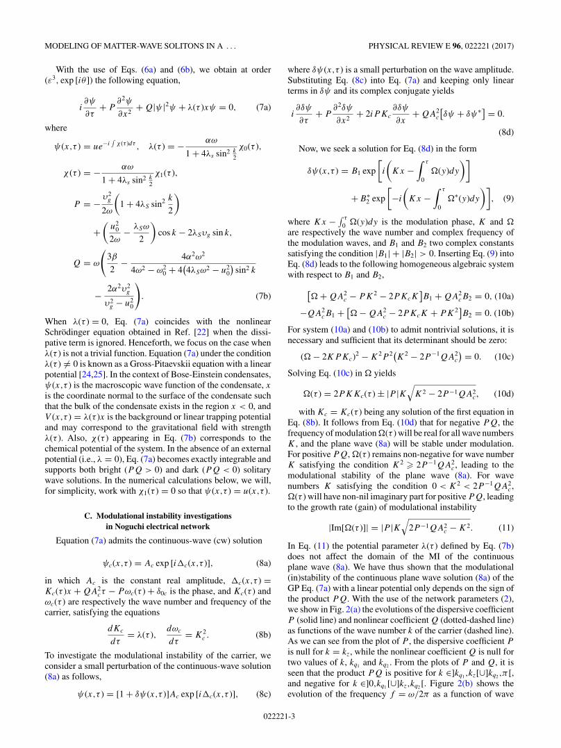
In Eq. (11) the potential parameter λ(τ ) defined by Eq. (7b)does not affect the domain of the MI of the continuousplane wave (8a). We have thus shown that the modulational(in)stability of the continuous plane wave solution (8a) of theGP Eq. (7a) with a linear potential only depends on the sign ofthe product PQ. With the use of the network parameters (2),we show in Fig. 2(a) the evolutions of the dispersive coefficientP (solid line) and nonlinear coefficient Q (dotted-dashed line)as functions of the wave number k of the carrier (dashed line).As we can see from the plot of P , the dispersive coefficient P

is null for k = kz, while the nonlinear coefficient Q is null fortwo values of k, kq1 and kq2 . From the plots of P and Q, it isseen that the product PQ is positive for k ∈]kq1 ,kz[∪]kq2 ,π [,and negative for k ∈]0,kq1 [∪]kz,kq2 [. Figure 2(b) shows theevolution of the frequency f = ω/2π as a function of wave

022221-3

E. KENGNE, A. LAKHSSASSI, AND W. M. LIU PHYSICAL REVIEW E 96, 022221 (2017)

FIG. 2. (a) Behavior of the dispersive coefficient P (solid line) and plots of the nonlinear coefficient Q (dotted-dashed line) as functions ofthe wave number k for network parameters (2). (b) Linear dispersive curve showing the evolution of the frequency f = ω/2π as a function ofthe wave number k for network parameters (2). Here, fz = ω(kz)/2π , fq1 = ω(kq1 )/2π , and fq2 = ω(kq2 )/2π , with kz and kq1 and kq1 beingrespectively the zeros of P (k) and Q(k).

number k. With the help of Fig. 2(a), we have divided, asone can see from Fig. 2(b), the frequency domain [f0,fmax]into four regions concerning the modulational instability ofthe plane wave and the possible soliton solutions of the GPEq. (7a): two regions of positive PQ (]fq1 ,fz[ and ]fq2,fmax])corresponding to the MI of the plane wave and leading toenvelope solitons, and two regions of negative PQ ([f0,fq1

[ and ]fz,fq2 [) corresponding to the modulational stability ofthe plane wave and leading to hole solitons.

III. ANALYTICAL INVESTIGATION OF SOLITONPROPAGATION IN THE NETWORK OF FIG. 1

With the help of the solitary wave solutions of the GPEq. (7a), we investigate in this section the propagation of bothbright (PQ > 0) and dark (PQ < 0) solitary waves in thenetwork of Fig. 1. To experience the propagation of solitarywaves through the model shown in Fig. 1 for several bandsof frequencies, we follow Marquie et al. [26] and excite theleft extremity of the network with a solitary wave solution ofthe GP Eq. (7a). To avoid signal reflection that disturbs theaccurate observation of the wave propagation in the line, thevoltage across the right extremity is set to zero.

A. Propagation of bright solitary voltage signalin the network of Fig. 1

The propagation of bright solitary waves in the networkof Fig. 1 is associated with the positivity of product PQ. Aswe have shown in the previous section, Eq. (7a) admits thecontinuous-wave solution

ψc(x,τ ) = Ac exp[i�c(x,τ )], (12a)

�c(x,τ ) = Kc(τ )x + A2cQτ − Pωc(τ ) + δ0c,

dKc

dτ= λ(τ ),

dωc

dτ= K2

c (τ ). (12b)

Using the cw solution (12a) and (12b) as a seed solution, wefollow Kengne and Talla [27] and look for bright solitonicwave solutions of Eq. (7a) in the form

ψ(x,τ ) = [Ac + �(x,τ )] exp [i�c(x,τ )], (13)

where �(x,τ ) is a complex function. Inserting Eq. (13) intoEq. (7a) yields

i∂�

∂τ+ P

∂2�

∂x2+ Q|�|2� + 2iPKc

∂�

∂x

+QA2c(� + �∗) + QAc(�2 + 2|�|2) = 0. (14)

Now, we seek solitary wave solutions of Eq. (14) in the form

�(x,τ ) = As

γ cosh ξ + cos ϕ + iμ sin ϕ

cosh ξ + γ cos ϕ, (15)

where As , γ , and μ are three real constants with μ �= 0,and ξ = ξ (x,τ ) and ϕ = ϕ(τ ) are two real functions to bedetermined. Asking that function (15) satisfies Eq. (14), weobtain for As �= 0, after some long calculations,

ξ (x,τ ) = Asμ

√Q

2P[x − 2Pυ(τ ) + ξ̃0],

ϕ(τ ) = A2sμ

Q

2Pτ + η0,

μ2 = A2s − 4A2

c

A2s

, γ = −2Ac

As

,dυ

dτ= Kc(τ ), (16)

under the condition A2s − 4A2

c > 0. Inserting Eq. (15) intoEq. (13), we obtain the following bright solitonic solution ofEq. (7a),

ψ(x,τ ) =(

Ac + As

γ cosh ξ + cos ϕ + iμ sin ϕ

cosh ξ + γ cos ϕ

)× exp [i�c(x,τ )]. (17)

where ξ , ϕ, γ , and μ are defined by Eq. (16). Insertingsolution (17) into Eq. (3) [we remember that χ1(τ ) = 0 sothat ψ(x,τ ) = u(x,τ )] and using Eqs. (6a) and (6b), we cananalytically instigate the propagation of bright solitary wavesin the network of Fig. 1.

022221-4

MODELING OF MATTER-WAVE SOLITONS IN A . . . PHYSICAL REVIEW E 96, 022221 (2017)

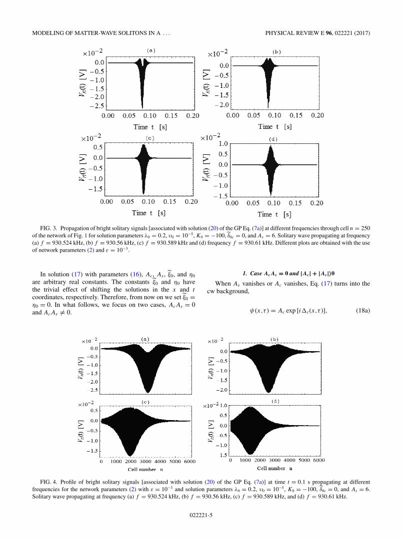
FIG. 3. Propagation of bright solitary signals [associated with solution (20) of the GP Eq. (7a)] at different frequencies through cell n = 250of the network of Fig. 1 for solution parameters λ0 = 0.2, υ0 = 10−5, K0 = −100, δ̃0c = 0, and As = 6. Solitary wave propagating at frequency(a) f = 930.524 kHz, (b) f = 930.56 kHz, (c) f = 930.589 kHz and (d) frequency f = 930.61 kHz. Different plots are obtained with the useof network parameters (2) and ε = 10−3.

In solution (17) with parameters (16), Ac, As , ξ̃0, and η0

are arbitrary real constants. The constants ξ̃0 and η0 havethe trivial effect of shifting the solutions in the x and t

coordinates, respectively. Therefore, from now on we set ξ̃0 =η0 = 0. In what follows, we focus on two cases, AcAs = 0and AcAs �= 0.

1. Case Ac As = 0 and |Ac| + |As|〉0

When As vanishes or Ac vanishes, Eq. (17) turns into thecw background,

ψ(x,τ ) = Ac exp [i�c(x,τ )], (18a)

FIG. 4. Profile of bright solitary signals [associated with solution (20) of the GP Eq. (7a)] at time t = 0.1 s propagating at differentfrequencies for the network parameters (2) with ε = 10−3 and solution parameters λ0 = 0.2, υ0 = 10−5, K0 = −100, δ̃0c = 0, and As = 6.Solitary wave propagating at frequency (a) f = 930.524 kHz, (b) f = 930.56 kHz, (c) f = 930.589 kHz, and (d) f = 930.61 kHz.

022221-5

E. KENGNE, A. LAKHSSASSI, AND W. M. LIU PHYSICAL REVIEW E 96, 022221 (2017)

FIG. 5. Bright solitary signal voltage (in V) as a function of cellnumber n of the network at times t = 0.105 s of the propagation ofa wave moving with different group velocities. Bright solitary wavemoving with (a) group velocity υg = 4993.44 cell/ms at carrier fre-quency f = 930.626 kHz, (b) group velocity υg = 16 355.4 cell/msat carrier frequency f = 930.6 kHz, and (c) group velocity υg =31 507.9 cell/ms at carrier frequency f = 930.524 kHz. To generatedifferent plots, we have used the same network and solutionparameters as in Figs. 3 and 4.

and into the bright soliton,

ψ(x,τ ) = As

cosh[As

√Q

2P[x − 2Pυ(τ )]

]× exp [i�c(x,τ ) ± iϕ], (18b)

respectively, where the analytical expression for υ(τ ) can beobtained by combining Eqs. (12b) and (16),

υ(τ ) =∫ τ

0

[∫ y

0λ(z)dz + K0

]dy + υ0, (18c)

with υ0 = υ(0) and K0 = Kc(0) being two arbitrary realconstants. Therefore, in general, the exact solution (17)describes a solitary wave embedded on a cw background[28], and when Ac � As , the background is small within theexistence of the bright soliton. It is seen from solution (18b)

that (i) As is the amplitude of the bright soliton, and (ii) thecenter of the bright soliton is ζ (τ ) = 2Pυ(τ ) and satisfies theequation

d2ζ

dτ 2+ 2κ(τ )ζ = 0, (19)

with κ(τ ) = − λ(τ )2υ(τ ) . Equation (19) means that the center of

mass of the wave packet behaves as a classical particle, andallows one to manipulate the motion of bright solitons in thenetwork by controlling the potential parameter λ(τ ). (iii) Thetrajectory of a given soliton peak is obtained from the conditionξ = 0, leading to x = 2Pυ(τ ). In what follows, we take someexamples to demonstrate the dynamics of bright solitons in thenetwork of Fig. 1 associated with different kinds of strengthλ(τ ).

First, we consider the time-independent linear potentialwith strength λ(τ ) = λ0 [see Eq. (7b)] and obtain the brightsoliton solution

ψ(x,τ ) = As

cosh[As

√Q

2P

(x − 2P

{λ02 τ 2 + K0τ + υ0

})]× exp [i�(x,τ )], (20)

where �(x,τ ) = [λ0τ + K0]x − P [ λ20

3 τ 3 + λ0K0τ2 + K2

0 τ ]+A2

sQ

2Pτ + δ̃0c. In this situation, the trajectory of a given

soliton peak is x(τ ) = Pλ0τ2 + 2PK0τ + 2Pυ0. The tra-

jectory is thus parabolic in time with an acceleration ofd2x/dτ 2 = 2Pλ0. Mathematically, the trajectory of a givensoliton peak will be concave left on (the curve is situated at theleft of the tangent at each of its points) if Pλ0 > 0 and concaveright on (the curve is situated at the right of the tangent at eachof its points) if Pλ0 < 0.

With the use of solution (20) of the GP Eq. (7a), we showrespectively in Figs. 3 and 4 the time evolution of solitarysignals at different frequencies through cell n = 250 of thenetwork of Fig. 1 and the solitary wave profiles at time t = 0.1 spropagating at different frequencies. As we can see from theseplots, the form of a solitary wave along both the time and spaceaxes depends on its frequency. Waves shown in plots (a)–(d) of

FIG. 6. Effects of strength λ(τ ) of the linear trapping potential on a bright solitary signal voltage propagating at a frequency f = 930.6 kHzthrough the network of Fig. 1. Plots of the left panel (I) show the profiles of a bright solitary signal voltage at time t = 0.115 s for (a) λ0 = 0.2,(b) λ0 = 108, and (c) λ0 = 1.5 × 108, while plots of the right panel (II) show the profiles of a bright solitary signal voltage at time t = 0.115 s for(a) λ0 = −0.2, (b) λ0 = −108, and (c) λ0 = −1.5 × 108. To generate different plots, we have used the same network and solution parametersas in Fig. 3.

022221-6

MODELING OF MATTER-WAVE SOLITONS IN A . . . PHYSICAL REVIEW E 96, 022221 (2017)

Figs. 3 and 4 propagate with group velocities υg = 31 507.9,25 446.3, 19 385.5, and 13 325.4 cell/ms, respectively. Theplots of Figs. 3 and 4 also show that the wave speed increaseswith the group velocity of the propagating wave. This behavioris well seen in Fig. 5. Figures 3–5 also reveal that the brightsolitary voltage oscillates symmetrically around the zero volt-age as the carrier frequency approaches the cutoff frequencyfmax = 930.628 kHz. Figure 6 shows the profiles at time t =0.115 s of bright solitary signal voltages obtained for differentstrengths λ(τ ) = λ0 of the linear trapping potential. The plotsof this figure reveal that (i) the bright solitary wave velocitydecreases as strength λ(τ ) = λ0 > 0 increases and λ(τ ) =λ0 < 0 decreases, and (ii) the bright solitary wave oscillatessymmetrically around the zero voltage for only small λ0. Thislast behavior is well seen in Fig. 6(d). The plots of Fig. 6 thus

show how much strength λ(τ ) = λ0 of the linear trappingpotential may affect the wave trajectory and its velocity. It isimportant to note that all carrier frequencies f used in Figs. 3–6are taken in the MI region satisfying the conditions P (k) <

0 and Q(k) < 0 (the rightmost region in Fig. 2). Therefore,Pλ0 > 0 for negative λ0 and Pλ0 < 0 for positive λ0.

Second, we consider the temporal periodic modulation ofthe linear potential with strength λ(τ ) = λ0(1 + m sin aτ ),where λ0 �= 0 and a �= 0 are any real numbers, and 0 < m < 1.According to Eqs. (12b) and (18c), we have Kc(τ ) =λ0(τ − m

acos aτ ) + K0, υ(τ ) = λ0( 1

2τ 2 − ma2 sin aτ ) +

K0τ + υ0, and ωc(τ ) = λ20

3 τ 3 + K0λ0τ2 + (K2

0 + λ20m

2

2a2 )τ −( 2K0λ0m

a2 + 2mλ20

a2 τ ) sin aτ − 2mλ20

a3 cos aτ + m2λ20

4a3 sin 2aτ + ωc0.According to Eq. (18b), we get the bright one-solitary wave

FIG. 7. Effects of the strength λ(τ ) on bright solitary waves propagating at a carrier frequency f = 930.626 kHz for the networkparameters (2) with ε = 10−3 and for the solution parameters [see Eq. (21)] υ0 = 15 × 10−6, K0 = −100, δ̃0 = ωc0 = 0. The top plots (I) and(II) respectively show the spatial evolution at time t = 0.022 s and the temporal evolution through cell n = 250 of a bright solitary signalvoltage in the network for m = 0.1, a = 0.2, and three values of parameter λ0: (a) λ0 = 1350, (b) λ0 = 1450, and (c) λ0 = 1550. The middleplots (III) and (IV) respectively show the spatial evolution at time t = 0.025 s and the temporal evolution through cell n = 250 of a brightsolitary signal voltage in the network for λ0 = 1500, m = 0.1, and three values of parameter a: (a) a = 0.2, (b) a = 0.22, and (c) a = 0.24.The bottom plots (V) and (VI) respectively show the spatial evolution at time t = 0.2 s and the temporal evolution through cell n = 250 ofa bright solitary signal voltage in the network for λ0 = 1500, a = 0.2, and three values of parameter m: (a) m = 0.11, (b) m = 0.12, and (c)m = 0.13.

022221-7

E. KENGNE, A. LAKHSSASSI, AND W. M. LIU PHYSICAL REVIEW E 96, 022221 (2017)

solution

ψ(x,τ ) = As

cosh[As

√Q

2P

(x − 2P

{λ02 τ 2 + K0τ − λ0m

a2 sin aτ + υ0})] exp [i�(x,τ )], (21)

where �(x,τ ) = Kc(τ )x + A2s

Q

2Pτ − Pωc(τ ) + δ̃0. In the

present situation, the trajectory of a given soliton peak isx(τ ) = Pλ0τ

2 + 2PK0τ − 2Pλ0m

a2 sin aτ + υ0.With the use of solution (21), we show in Fig. 7, for different

parameters of the strength λ(τ ), the spatial (left panels) andtemporal (right panel) evolution of the bright solitary signalvoltage. The top, middle, and bottom plots are obtained withdifferent values of λ0, a, and m, respectively. Plot (I) showsthat the bright solitary wave oscillates symmetrically aroundthe zero voltage with a velocity that increases with λ0, whileplot (II) reveals that the lifetime of a bright solitary signalthrough a given cell increases as the parameter λ0 decreases.Comparing the top and middle plots, we conclude that λ0 and

a have opposite effects on the propagation of bright solitarywaves through the network. It is seen from the top and bottomplots that parameters λ0 and m have the same effect as thewave propagation; indeed, when parameter a is chosen suchthat sin aτ remains positive, the strength λ(τ ) of the trappingpotential increases with each λ0 and m.

2. Case Ac As �= 0

Here, we investigate the situation when solution (17)with parameters (16) describes solitary waves embedded oncontinuous-wave backgrounds. Let us rewrite solution (17)here,

ψ(x,τ ) =(

Ac + As

−2Ac cosh ξ + As cos ϕ ± i√

A2s − 4A2

c sin ϕ

As cosh ξ − 2Ac cos ϕ

)exp [i�c(x,τ )], (22a)

ξ (x,τ ) = As

√Q

(A2

s − 4A2c

)2PA2

s

[x − 2Pυ(τ )], ϕ(τ ) = As

√A2

s − 4A2c

Q

2Pτ . (22b)

An analysis of Eqs. (22a) and (22b) reveals that the velocityfor the solitary wave still satisfies Eq. (19). In particular, whenλ(τ ) = λ0 exp [aτ ] with real parameters λ0 and a satisfying thecondition λ0a �= 0, we find υ(τ ) = λ0

a2 exp [aτ ] + Kc0τ + υ0

and �c(x,τ ) = ( λ0a

exp [aτ ] + Kc0)x + (QA2c − PK2

c0)τ −P ( 2Kc0λ0

a2 exp [aτ ] + λ20

2a3 exp [2aτ ]) + �c0, with Kc0, υ0,and �c0 being three arbitrary real constants. For thenetwork parameters (2), ε = 10−2, for solution parameters�c0 = ωc0 = 0, Kc0 = 2 × 10−5, υ0 = 0, As = 1, and for thestrength λ = 570 exp [−12t] (that is, λ0 = 570 and a = −12),we show in Fig. 8, for different values of Ac, the propagation ofbright solitary voltage signals embedded on continuous-wavebackgrounds. In Figs. 8(a) and 8(b), Ac = 10−3 � 1 = As

and the background is neglected (invisible) within the

existence of the bright solitary wave. In Figs. 8(c) and 8(d),Ac = 0.1 = As/10 and the background is small (but visible)within the existence of the bright solitary wave. In Figs. 8(e)and 8(f), Ac = 0.499 As/2 and the background is largewithin the existence of the bright solitary wave.

B. Propagation of dark solitary voltage signalin the network of Fig. 1

Now, we consider the case when PQ < 0, leading toa dark soliton solution of the GP Eq. (7a). In this case,we seek a dark soliton solution of Eq. (7a) in the formψd (x,τ ) = (Ac + iAs tanh [y(x,τ )]) exp [iKd (τ )x + i�d (τ )],where y(x,τ ) = ρ0x + y0(τ ), Kd (τ ), and �d (τ ) are functionsto be determined, and ρ0, ρc, and ρs are three real parameters.Asking that ψd (x,τ ) satisfies Eq. (7a) leads to

ψd (x,τ ) =√

−2P

Q

(ρc ± iρs tanh

[ρs

(x ±

√− Q

2Py0(t)

)])exp [iKd (τ )x + i�d (τ )], (23)

dKd

dτ= λ(τ ), (24)

d�d

dτ= −2P

(ρ2

c − ρ2s

) − PK2d , (25)

dy0

dτ= −2P

√− Q

2P(ρc ± Kd ), (26)

022221-8

MODELING OF MATTER-WAVE SOLITONS IN A . . . PHYSICAL REVIEW E 96, 022221 (2017)

FIG. 8. Propagation at frequency f = 930.62 kHz of bright solitary voltage signals associated with the solitary wave embedded on acontinuous-wave background (22a) and (22b) for different values of the solution parameter Ac: (a), (b) Ac = 10−3; (c), (d) Ac = 0.1; (e), (f)Ac = 0.499. The left plots show the evolution of solitary bright signals embedded on continuous-wave backgrounds through cell n = 600.The right plots show the spatial profile at time t = 0.1 s of solitary bright signals embedded on continuous-wave backgrounds in the network.Different parameters used to generate these plots are given in the text.

where ρs = As

√− Q

2Pand ρc = Ac

√− Q

2P. When

ρs = 0 or ρc = 0, ψd (x,τ ) reduces respectively to the

background ψd (x,τ ) = ρc

√− 2P

Qexp [iKd (τ )x + i�d (τ )]

and the dark solitary wave ψd (x,τ ) = ±iρs

√− 2P

Q

tanh [ρs(x ±√

− 2PQ

y0(t))] exp[iKd (τ )x +i�d (τ )]. Thus,

ψd (x,τ ) represents a dark solitary wave embedded in thebackground. It is seen from Eq. (23) that the amplitude ofthe dark soliton is proportional to

√−2P/Q, while the widthis inversely proportional to

√−2P/Q. Thus Eq. (23) canbe used to describe the compression of dark solitary waveswhen

√−Q/2P increases with the wave number k. Becauseof the relationships between λ(τ ) and Kd [see Eq. (24)], thesoliton speed υd (τ ) = dx/dτ = ∓Q(ρc ± Kd ) is intimatelydependent on the potential parameter λ(τ ). In our numericalsimulation, we focus on the case with the “+” sign in Eqs. (23)and (26).

Inserting solution (23) into Eq. (3) [we remember thatχ1(τ ) = 0 so that ψ(x,τ ) = u(x,τ )] and using Eqs. (6a)and (6b), we can analytically instigate the evolution ofa dark solitary voltage signal in the network of Fig. 1when the wave frequencies are taken from the region

of modulational stability of the plane wave, i.e., whenproduct PQ is negative. In the special case of a time-independent linear trap potential, that is, when λ(τ ) = λ0

is a nonzero constant, Eqs. (24)–(26) lead to Kd (τ ) =λ0τ + Kd0, �d (τ ) = −2P (ρ2

c − ρ2s )τ − P

3λ0(λ0τ + Kd0)3 +

�d0, and y0(τ ) = −2P

√− Q

2P(ρcτ + 1

2λ0(λ0τ + Kd0)2) + y00,

where Kd0, �d0, and y00 are three arbitrary real constants.In this situation, the soliton speed is υd (τ ) = −Qλ0τ −Q(ρc + Kd0). Depending on the size and the sign of the poten-tial parameter λ0, the soliton speed υd (τ ) can either be positiveduring its propagation or negative during its propagation.

The main parameters appearing in solution (23)–(26) inthe special case λ(τ ) = λ0 �= 0 are the wave amplitudes ρc

and ρs , the wave numbers k = kp leading to the propagatingfrequencies f = fp = ω(kp)/2π , and the potential parameterλ0. Other free parameters Kd0, �d0, and y00 appear whenintegrating Eqs. (24)–(26). Figures 9–11 show the timeevolutions of a dark solitary voltage signal through celln = 350 of the network for respectively different Ac and As ,different wave numbers k, and different values of parametersλ. As it is seen from these figures, each main parameter ρc, ρs ,k, and λ0 leads to a particular profile of a dark solitary wavepropagating through the network. Each of these three figures

022221-9

E. KENGNE, A. LAKHSSASSI, AND W. M. LIU PHYSICAL REVIEW E 96, 022221 (2017)

FIG. 9. Effects of the continuous-wave background on a dark solitary voltage signal propagating through cell n = 350 at frequencyf = fp = 381.655 kHz for ρs = 0.121 39, λ0 = 0.1, y00 = 11.2, Kd0 = 10−5, �d0 = 0, and (a) ρc = 0, (b) ρc = 0.060 694 9, (c) ρc = 0.121 39,and (d) ρc = 0.182 085.

is obtained with the use of the network parameters (2) andε = 10−2. Figure 9 shows the effects of the continuous-wavebackground on a dark solitary wave. Figure 9(a) shows a darksolitary wave propagating on a vanishing continuous-wavebackground, i.e., when ρc = 0. Figures 9(b)–9(d) show darksolitary waves embedded on a continuous-wave backgroundwith respectively ρc < ρs , ρc = ρs , and ρc > ρs . The plots ofFig. 9 show that the depth of the dark soliton decreases asthe parameter ρc of the background increases. It is seen fromFigs. 9(a)–9(d) that when ρc � ρs or ρs � ρc, the backgroundis small within the existence of a dark soliton or the dark solitonis small within the existence of a continuous-wave background.Figure 10 shows how much the carrier frequency f = fp

impacts the behavior of dark solitary waves embedded oncontinuous-wave backgrounds during its propagation througha given cell of the network. The change in the behavior(deformation) of the wave with its carrier frequency is dueto the coefficient of u2 in the expression of the second-harmonic terms ψ2 given by Eq. (6b). The effects of thepotential parameter λ = λ0 on dark solitons embedded oncontinuous-wave backgrounds are shown in Fig. 11, showingthe time evolution of the dark solitary voltage signal forpositive (top plots) and negative (bottom plots) values of theparameter λ0. The top and bottom plots show that the velocityof the dark soliton decreases when the potential parameter λ0

increases.

FIG. 10. Influence of the carrier frequency on wave behavior during its propagation through cell n = 350 of the network for ρs

√− 2P

Q= 1,

ρc

√− 2P

Q= 0.5, λ0 = 0.1, y00 = 11.2, Kd0 = 10−5, �d0 = 0. (a) Time evolution of a dark soliton embedded on a continuous-wave background

for the frequency f = fp = 381.655 kHz, (b) f = fp = 381.658 kHz, (c) f = fp = 381.679 kHz, and (d) f = fp = 381.74 kHz.

022221-10

MODELING OF MATTER-WAVE SOLITONS IN A . . . PHYSICAL REVIEW E 96, 022221 (2017)

FIG. 11. Effects of the linear trap potential parameter λ = λ0 on dark solitary waves propagating at a frequency f = fp = 381.656 kHzthrough cell n = 350 of the network for ρs = 0.121 39, ρc = 0.036 417, y00 = 11.2, Kd0 = 10−5, �d0 = 0. The top plots show the timeevolution of dark soliton for positive λ0: (a) λ0 = 10, (b) λ0 = 5000, and (c) λ0 = 104. The bottom plots show the time evolution of a darksoliton for positive λ0: (d) λ0 = −10, (e) λ0 = −500, and (f) λ0 = −103.

One of the features of Fig. 11 is that the behavior ofthe dark soliton shown in Fig. 11(f) is different from thatof other waves [Figs. 11(a)–11(e)]. Does Fig. 11(f) showan interaction of two dark solitons embedded on the samecontinuous-wave background? Our numerical computationshave shown that the wave behavior in Fig. 11(f) occurs formany other λ0 ∈ [λ01,λ02], where λ01 < −100 < λ02. As wecan see from Fig. 12, the behavior shown in Fig. 11(f) alsodepends on ρc.

C. Experimental validation

Suppose we have a pulse generator, for example, a pro-grammable generator that allows us to create highly custompulse shapes by varying the amplitude at various points.Moreover, suppose we have a numerical oscilloscope XSC1which has a high impedance that is used to avoid signalreflection. Then, for the experimental validation of our results,one can follow Marquie et al. [26] and consider a nonlinearelectrical network with N = 45 identical cells in which each

FIG. 12. Impacts of the continuous-wave background on the behavior of dark solitary voltage signals propagating through cell n = 350at frequency f = fp = 381.656 kHz for ρs = 0.121 39, λ0 = −103, y00 = 11.2, Kd0 = 10−5, �d0 = 0, and (a) ρc = 0.036 417, (b) ρc =0.012 139, (c) ρc = 0.001 213 9, and (d) ρc = 0.

022221-11

E. KENGNE, A. LAKHSSASSI, AND W. M. LIU PHYSICAL REVIEW E 96, 022221 (2017)

diode BB112 is biased by Vb = 2 V, and matched by a resistorin order to simulate an infinite line. The waves are then createdby using the programmable generator, and the wave formsare observed and stored by using the numerical oscilloscopeXSC1. After finding the best shape for unaltered propagation(soliton), this could be compared to our theoretical results.

IV. CONCLUSION

In this paper, we have considered a modified Noguchielectrical network and, by applying the reductive perturbationmethod in the semidiscrete limit, we have showed thatthe dynamics of the modulated waves in the network canbe governed by a Gross-Pitaevskii equation with a time-dependent linear potential in the presence of a chemicalpotential. We have shown that the potential parameter doesnot affect the growth rate (gain) of the MI of our system.

We have found exact analytical solitary wave solutions ofthe GP equation with derived time-dependent linear potentialsfor both cases of modulational instability and modulationalstability of our system. Using these exact analytical solutions,we have investigated numerically the transmission of bothbright and dark solitary voltage signals in the network, andthe effects of the potential parameter as well as those of thecarrier frequency on the propagation of solitary voltage wavesembedded on cw backgrounds in the network. Our studiesshowed that the behavior of solitary waves propagating inthe network simultaneously depend on the wave frequency,on the potential parameter, and on the amplitude of the cwbackground. Our exact analytical solitary wave solutions canbe useful for investigating the dynamics of modulated wavesin other physical systems described by a GP equation witha time-dependent linear potential, such as one-dimensionalBose-Einstein condensates.

[1] A. C. Scott, Nonlinear Science: Emergence and Dynamics ofCoherent Structures (Oxford University Press, New York, 1999).

[2] A. Hasegawa, Optical Solitons in Fibers, 2nd ed. (Springer,Berlin, 1989).

[3] M. Remoissenet, Waves Called Solitons, 3rd ed. (Springer,Berlin, 1999).

[4] N. J. Zabusky and M. D. Kruskal, Phys. Rev. Lett. 15, 240(1965).

[5] K. Lonngren, in Solitons in Action, edited by K. Lonngren andA. Scott (Academic, New York, 1978).

[6] T. Taniuti and N. Yajima, J. Math. Phys. 10, 1369 (1969).[7] F. II Ndzana, A. Mohamadou, T. C. Kofané, and L. Q. English,

Phys. Rev. E 78, 016606 (2008).[8] F. B. Pelap, J. H. Kamga, S. B. Yamgoue, S. M. Ngounou, and

J. E. Ndecfo, Phys. Rev. E 91, 022925 (2015).[9] E. Kengne, V. Bozic, M. Viana, and R. Vaillancourt, Phys. Rev.

E 78, 026603 (2008).[10] T. Kakutani and N. Yamasaki, J. Phys. Soc. Jpn. 45, 674 (1978).[11] A. C. Newell and J. V. Moloney, Nonlinear Optics (Addison-

Wesley, Boston, 1991).[12] F. S. Yamasaki, L. P. S. Neto, J. O. Rossi, and J. J. Barroso, IEEE

Trans. Plasma Sci. 42, 3471 (2014).[13] R. Hirota and K. Suzuki, Proc. IEEE 61, 1483 (1973).[14] A. C. Scott, Active and Nonlinear Wave Propagation in

Electronics (Wiley-Interscience, New York, 1970).

[15] R. Marquié, J. M. Bilbault, and M. Remoissenet, Physica D 87,371 (1995).

[16] H. Malwe Boudoue, B. Gambo, S. Y. Dokab, and T. CrepinKofane, Appl. Math. Comput. 239, 299 (2014).

[17] E. Afshari and A. Hajimiri, IEEE J. Solid-State Circ. 40, 744(2005).

[18] E. Kengne and W. M. Liu, Phys. Rev. E 73, 026603 (2006).[19] D. Yemélé and F. Kenmogné, Phys. Lett. A 373, 3801

(2009).[20] D. Ndjanfang, D. Yemélé, P. Marquié, and T. C. Kofané, Prog.

Electromagn. Res. B 52, 207 (2013).[21] X. Oriols and F. Martín, J. Appl. Phys. 90, 2595 (2001).[22] E. Kengne, A. Lakhssassi, and W. M. Liu, Phys. Rev. E 91,

062915 (2015).[23] M. Remoissenet, Waves Called Solitons, 2nd ed. (Springer,

Berlin, 1996).[24] E. Lundh, C. J. Pethick, and H. Smith, Phys. Rev. A 55, 2126

(1997).[25] U. Al Khawaja, C. J. Pethick, and H. Smith, Phys. Rev. A 60,

1507 (1999).[26] P. Marquie, J. M. Bilbault, and M. Remoissenet, Phys. Rev. E

49, 828 (1994).[27] E. Kengne and P. K. Talla, J. Phys. B: At. Mol. Opt. Phys. 39,

3679 (2006).[28] L. Wu, J.-F. Zhang, and L. Li, New J. Phys. 9, 69 (2007).

022221-12