Embed Size (px)
Citation preview

Modeling of Lithium-ion Battery
Performance and Thermal Behavior in
Electrified Vehicles
by
Ehsan Samadani
A thesis
presented to the University of Waterloo
in fulfillment of the
thesis requirement for the degree of
Doctor of Philosophy
in
Mechanical Engineering
Waterloo, Ontario, Canada, 2015
© Ehsan Samadani 2015

ii
AUTHOR'S DECLARATION
I hereby declare that this thesis consists of material which I mainly authored or co-authored. This
is a true copy of the thesis, including any required final revisions, as accepted by my examiners.
I understand that my thesis may be made electronically available to the public.

iii
Abstract
Electric vehicles (EVs) have received significant attention over the past few years as a
sustainable and efficient green transportation alternative. However, severe challenges, such as
range anxiety, battery cost, and safety, hinder EV market expansion. A practical means to reduce
these barriers is to improve the design of the battery management system (BMS) to accurately
estimate the battery state of charge (SOC) and state of health (SOH) in addition to
communicating with other powertrain components. Along with a robust estimation strategy, a
critical requirement in developing an efficient BMS is a high fidelity battery model to predict the
battery voltage, SOC, and heat generation profile at various temperature and power demands.
Such a model should also be able to capture battery degradation, which is a path-dependent
parameter that affects the battery performance in terms of output voltage, power capability and
heat generation. In this thesis, the Li-ion battery, a proven technology for electrified vehicles, is
studied under different operation scenarios on a plug-in hybrid vehicle (PHEV). The following
steps have been accomplished:
1- Development of a data-driven battery thermal model: A set of thermal characterization
tests are conducted on Li-ion cells. Heat generation profiles of each battery are driven for
a set of operating points including various ambient temperatures, states of charge (SOCs)
and load profiles. A regression model is developed accordingly which is able to accurately
predict the battery temperature during a driving or charging event. The model shows an
average error of 4% in temperature predictions.
2- Development of a data-driven battery performance model for real-time on-board
applications: An equivalent circuit model is developed based on the electrochemical
impedance spectroscopy (EIS) tests. This model can precisely predict the battery
operating voltage under various operating conditions. An overall 6% improvement is
observed in voltage prediction compared to common models in the literature. Results also
show, depending on the powertrain designer expected accuracy, that this model can be
used to predict the battery internal resistance obtained from hybrid pulse power
characterization (HPPC) tests.

iv
3- Battery degradation studies through field tests: An electrified Ford Escape vehicle is
tested through random and controlled driving and charging events and battery data is
collected and analyzed to identify trends of degradation including capacity fade and power
fade. A battery life model is recalibrated based on the measured battery capacities over the
field test period. Although, data shortage and technical issues prevented this study from
meeting its targeted scope, the presented analysis provides a pathway for future research.
4- Battery lifetime modeling: fuel consumption, all-electric range and battery capacity loss
are simulated under various scenarios including different climate control loads, ambient
conditions, powertrain architectures and battery preconditioning. To simulate the climate
control loads impact, a vehicle cabin thermal model is developed that incorporates the
ambient conditions to predict the temperature profile of the cabin and the cooling/heating
load required to regulate the temperature. Accordingly, this load is translated into
additional load on the battery, which enables assessment of its impacts on the battery life,
fuel consumption and vehicle range.

v
Acknowledgements
I would like to express my sincere gratitude to Prof. Fraser and Prof. Fowler, for their
constant guidance, and support during the course of this research. I would also like to thank
people at Burlington Hydro Co., Cross Chasm Co. and also my friends, Dr. Siamak Farhad,
Satyam Panchal and Mehrdad Mastali for providing assistance and constructive feedback. Last
but not least, my special gratitude to my lovely wife, Ensieh, for her continuous love and support
during these years.

vi
To those who sacrificed to make this world a better place to live…

vii
Table of Contents
AUTHOR'S DECLARATION ....................................................................................................... ii
Abstract .......................................................................................................................................... iii
Acknowledgements ......................................................................................................................... v
Table of Contents .......................................................................................................................... vii
List of Figures ................................................................................................................................ xi
List of Tables ................................................................................................................................ xv
1 Introduction ................................................................................................................................ 1
1.1 Problem definition and research objectives ......................................................................... 4
1.1.1 Battery Performance Modeling .................................................................................. 4
1.1.2 Battery Thermal Characterization .............................................................................. 6
1.1.3 Battery Degradation ................................................................................................... 7
1.1.4 Auxiliary Loads in EVs .............................................................................................. 7
1.2 Document Organization ....................................................................................................... 8
2 Background and literature review ............................................................................................ 10
2.1 Battery Elements and Specificationds ................................................................................ 10
2.1.1 Anode ....................................................................................................................... 10
2.1.2 Cathode .................................................................................................................... 10
2.1.3 Electrolyte ................................................................................................................ 10
2.1.4 Separator .................................................................................................................. 11
2.2 Battery Gloassary ............................................................................................................... 11
2.2.1 Battery Management System ................................................................................... 11
2.2.2 State of Charge ......................................................................................................... 12
2.2.3 Depth of Discharge- ................................................................................................. 12
2.2.4 C-rate ........................................................................................................................ 12
2.2.5 Cell Capacity ............................................................................................................ 12
2.2.6 Cycle ........................................................................................................................ 13
2.2.7 Cell Open Circuit Voltage ........................................................................................ 13
2.2.8 Internal Resistance ................................................................................................... 14
viii
2.3 Electric Vehicles Battery Types ......................................................................................... 16
2.4 Li-ion Cell Operation ......................................................................................................... 19
2.5 Battery Models ................................................................................................................... 21
2.5.1 Electrochemical Models ........................................................................................... 21
2.5.2 Equivalent Circuit Models ....................................................................................... 21
2.6 Battery Degradation Modeling ........................................................................................... 25
2.7 Degradation Mechanisms of Li-ion Cells .......................................................................... 26
2.7.1 Degradation under Storage (i.e. Calendar Aging) .................................................... 26
2.7.2 Degradation during Cycling ..................................................................................... 27
2.8 Accelerated Degradation during Cycling ........................................................................... 29
2.9 Duty cycle & Drive cycle ................................................................................................... 32
2.10 PHEV and HEV Considerations ...................................................................................... 33
3 Modeling of Battery Thermal Behavior and Performance ...................................................... 36
3.1 Thermal Characterization ................................................................................................... 36
3.1.1 Experimental setup ................................................................................................... 37
3.1.2 Analysis of results .................................................................................................... 41
3.2 Modeling of Battery Performnce Based on EIS Tests ....................................................... 60
3.2.1 Experiment Setup and Tests Procedure ................................................................... 61
3.2.2 Establishment of the Equivalent Circuit .................................................................. 63
3.2.3 Parameters Fitting .................................................................................................... 68
3.2.4 Determination of the Voltage Response in Time Domain ....................................... 70
3.2.5 Results and Discussion ............................................................................................. 74
3.2.6 Impact of convection coefficient on the temperature profile ................................... 82
3.3 Conclusions ........................................................................................................................ 83
4 Battery Characterization through Field Tests .......................................................................... 85
4.1 Data Management System and Battery Packs .................................................................... 86
4.2 Results and Analysis .......................................................................................................... 88
4.2.1 Individual Event Analysis ........................................................................................ 88
4.2.2 Energy and Cost Analysis of EV-ACX 2.5 .............................................................. 91
ix
4.3 Vehicle Powertrain Modeling ............................................................................................ 96
4.3.1 Estimation of the Battery OCV and Internal Resistance .......................................... 98
4.3.2 Model Testing and Validation ................................................................................ 101
4.3.3 Case study- Testing the proposed ECM with a Real-life drive cycle .................... 112
4.3.4 Overall Powertrain Efficiency of EV-ACX2.5 ...................................................... 115
4.3.5 Energy Requirement of EV-ACX2.5 as a Fleet Vehicle ....................................... 117
4.3.6 Studies on Battery Degradation ............................................................................. 118
4.4 Conclusion ........................................................................................................................ 132
5 Modeling of Battery Lifetime in Hybrid Vehicle Operation ................................................. 134
5.1 Range Anxiety and Auxiliary loads in PEVs ................................................................... 134
5.2 Cabin Thermal Model ...................................................................................................... 135
5.3 Climate Scenarios ............................................................................................................. 140
5.4 Results- Thermal model and A/C impacts ....................................................................... 140
5.5 Vehicle Simulations ......................................................................................................... 142
5.5.1 CD range and Fuel consumption ............................................................................ 143
5.5.2 Degradation simulation .......................................................................................... 145
5.6 Conclusions ...................................................................................................................... 148
6 Conclusions and Recommendations ...................................................................................... 150
6.1 Conclusions and Contributions ........................................................................................ 150
6.1.1 Thermal studies ...................................................................................................... 150
6.1.2 EIS Tests and Modeling ......................................................................................... 151
6.1.3 Field tests ............................................................................................................... 151
6.1.4 Vehicle lifetime studies .......................................................................................... 153
6.2 Recommendations ............................................................................................................ 153
6.2.1 Thermal testing....................................................................................................... 154
6.2.2 EIS testing .............................................................................................................. 154
6.2.3 Field testing ............................................................................................................ 155
6.2.4 Battery lifetime modeling ...................................................................................... 156
References ................................................................................................................................... 157

x
Appendix-A Statistical Analysis of Cell Temperature Distribution ........................................... 165
Appendix-B Derived Regression Models for the Circuit Parameters ......................................... 168
Appendix-C Modification on the driver model in Autonomie ................................................... 171
Appendix-D Monthly Report of EV-ACX2.5 ............................................................................ 172
xi
List of Figures
Figure1-1. Power flow in a series HEV powertrain [5] .................................................................... 2
Figure1-2. Power flow in a parallel HEV powertrain [5] ................................................................. 3
Figure1-3. Power flow in a series parallel HEV powertrain [5] ....................................................... 3
Figure 2-1 Li-ion battery OCV variation against SOC [45] ............................................................. 14
Figure 2-2 Lead acid battery OCV variation against SOC [46]....................................................... 14
Figure 2-3. Typical polarization of a battery [50] ......................................................................... 16
Figure 2-4. The Ragone plot of various cell types capable of meeting the requirements for EV
applications [53] . .......................................................................................................................... 18
Figure 2-5. Comparison of suitable Li-ions for EV. The more the colored shape extends along a
given axis, the better the performance in that direction [56]. ..................................................... 19
Figure 2-6.Charge and discharge process in Li-ion battery [58] ................................................... 20
Figure 2-7 Types of Li-ion cell formats: cylindrical, prismatic and pouch cell. ............................. 20
Figure 2-8 Rint model equivalent circuit diagram ........................................................................ 22
Figure 2-9 RC model equivalent circuit diagram .......................................................................... 23
Figure 2-10 Thevenin model equivalent circuit diagram [66] ...................................................... 23
Figure 2-11 DP model equivalent circuit diagram [65]. ................................................................ 24
Figure 2-12 Expanded DP model equivalent circuit diagram ....................................................... 24
Figure 2-13 EDP model components correlated with EIS results [19] .......................................... 25
Figure 2-14. The general shape for capacity versus cycle number [70]. ...................................... 27
Figure 2-15.Schematic of SEI film layer in Li-ion battery [71] ...................................................... 28
Figure 2-16. Cycle life vs. ΔDoD curve for different battery cell chemistries[75] ........................ 30
Figure 2-17. Example-Battery cell’s temperature range for optimal cycle life [76] ..................... 30
Figure 2-18. The accelerated capacity fading due to high temperatures [78] ............................. 31
Figure 2-19- Schematic of a driving cycle broken down into a series of sequential isolated
“driving pulses” or “micro trip” .................................................................................................... 33
Figure 3-1: Battery cycling test bench .......................................................................................... 38
Figure 3-2: Battery setup in thermal chamber ............................................................................. 39
Figure 3-3: Thermocouple placement on cell surface .................................................................. 40
Figure 3-4: A two factor NFCD used for thermal studies .............................................................. 41
Figure 3-5: LiFePO4 Cell temperature changes during rest period at 23.75 °C- measured against
fitted values .................................................................................................................................. 45
Figure 3-6: LiFePO4 cell temperature changes during discharge cycles ....................................... 46
Figure 3-7: LiFePO4 cell temperature changes during charge cycles ............................................ 46
Figure 3-8: LiMn2O4 cell temperature changes during discharge cycles ...................................... 47
xii
Figure 3-9: LiMn2O4 cell temperature changes during charge cycles ........................................... 47
Figure 3-10: LiFePO4 cell cumulative heat during discharge cycles .............................................. 48
Figure 3-11: LiFePO4 cell cumulative heat during charge cycles ................................................ 49
Figure 3-12: LIMn2O4 cell cumulative heat during discharge cycles ............................................. 49
Figure 3-13: LiMn2O4 cell cumulative heat during charge cycles ................................................. 50
Figure 3-14 Residuals showing a trend (variable variance) [88] ................................................... 57
Figure 3-15 Temperature profile of cell #1 (LiFePO4) during discharge at 2.5 C-rate and 23.75 ᵒC
ambient ......................................................................................................................................... 58
Figure 3-16 Temperature profile of cell #1 (LiFePO4) during discharge at 1.75 C-rate and 12.5 ᵒC
ambient ......................................................................................................................................... 58
Figure 3-17 Temperature profile of cell #1 (LiFePO4) under US06 profile and 12.5 ᵒC ambient . 59
Figure 3-18 Temperature profile of cell #1 (LiFePO4) under US06 profile and 35 ᵒC ambient .... 59
Figure 3-19: Experimental setup for the EIS test. ......................................................................... 62
Figure 3-20 EIS test results of battery #1 with LiFePO4 cathode 12.5 ᵒC ..................................... 64
Figure 3-21 EIS test results of battery #1 with LiFePO4 cathode 23.75 ᵒC ................................... 64
Figure 3-22 EIS test results of battery #1 with LiFePO4 cathode 35 ᵒC ........................................ 65
Figure 3-23 EIS test results of battery #1 with LiMn2O4 ............................................................... 65
Figure 3-24 EIS test results of battery #1 with LiMn2O4 ............................................................... 66
Figure 3-25 EIS test results of battery #1 with LiMn2O4 ............................................................... 66
Figure 3-26 Examples of the EIS plots showing two semicircles justifying the need for CPE
element in the circuit structure .................................................................................................... 67
Figure 3-27. Proposed equivalent circuit in frequency domain ................................................... 68
Figure 3-28. Simplification of the proposed circuit for time domain solution. ............................ 68
Figure 3-29. Fitted values of R1 for battery #1 ............................................................................. 70
Figure 3-30 Fitted values of R1 for battery #2 .............................................................................. 70
Figure 3-31 : HPPC test- pulse power characterization profile .................................................... 75
Figure 3-32. Comparison of discharge resistances obtained from HPPC tests and modeling for
the battery with LFP cathode at different temperatures. ............................................................ 77
Figure 3-33. Comparison of the battery voltage obtained from the empirical model and
experiment for the battery with LFP cathode at 35°C standard EPA drive cycles. ...................... 78
Figure 3-34. Comparison of discharge resistances obtained from HPPC tests and modeling for
the battery with composite LMO & NMC cathode at different temperatures. ........................... 81
Figure 3-35 Simulation of temperature profile under EPA drive cycles; (1)-(3): Impact of
convection coefficient on the temperature, (4) maximum temperature change as a function of
convection coefficient ................................................................................................................... 83
Figure 4-1 Converted Ford Escape (EV-ACX2.5) ........................................................................... 87

xiii
Figure 4-2. integration of multiple batteries packs [110] ............................................................. 87
Figure 4-3: Data recorder unit ...................................................................................................... 87
Figure 4-4: Data logger connection and shut down wire ............................................................. 87
Figure 4-5: Drive cycle for longest recorded trip with EV-ACX2.5 ................................................ 88
Figure 4-6: Acceleration profile for longest recorded trip with EV-ACX2.5 ................................. 88
Figure 4-7: Battery voltage profile for longest recorded trip with EV-ACX2.5 ............................. 90
Figure 4-8: Battery current profile for longest recorded trip with EV-ACX2.5 ............................. 90
Figure 4-9: Battery SOC profile for longest recorded trip with EV-ACX2.5 .................................. 90
Figure 4-10: Battery temperature profile for longest recorded trip with EV-ACX2.5 .................. 91
Figure 4-11: ACX 2.5 November 2011 monthly report [111] ....................................................... 94
Figure 4-12 Drivetrain configuration of the converted EV in PSAT [111] ..................................... 97
Figure 4-13 Top level of the battery model in PSAT ..................................................................... 97
Figure 4-14. Drive cycle #1 Synthesized for calibrating the battery model .................................. 98
Figure 4-15: Sample battery pack voltage profile ......................................................................... 99
Figure 4-16: Comparison of OCVs estimated from the road test and measured after 2hr resting
time. ............................................................................................................................................ 100
Figure 4-17: Internal resistance of the battery module derived from data of drive cycle #1 .... 101
Figure 4-18: SOC versus time; obtained from the model and drive cycle #1 ............................. 102
Figure 4-19: Power Flow into the Electric Motor, model and drive cycle #1 (first 8000 sec) .... 103
Figure 4-20. Inputs and Outputs to the Electric Motor .............................................................. 103
Figure 4-21. Vehicle Longitudinal Acceleration; drive cycle #1 (first 8000 sec) ......................... 104
Figure 4-22: Drive cycle #2 used for testing the model .............................................................. 104
Figure 4-23: SOC versus time; obtained from the model and field test related to drive cycle #2.
..................................................................................................................................................... 105
Figure 4-24. Input Power from Electric Motor; Test Drive Cycle(Dec7-Part1) ........................... 106
Figure 4-25. Vehicle Longitudinal Acceleration; Test Drive Cycle(Dec7-Part1) .......................... 106
Figure 4-26: Drive cycle #3 .......................................................................................................... 107
Figure 4-27: Frequency of the Battery pack C-rates for the drive cycle #3 ................................ 108
Figure 4-28: Battery SOC Validation Against drive cycle #3 ....................................................... 109
Figure 4-29: Battery Model Validation against Test Data over Drive cycle #3 ........................... 109
Figure 4-30: The coefficient of d(OCV)/dT versus SOC for the single cell of the battery back
under study [48]. ......................................................................................................................... 110
Figure 4-31: Reversible heat generated during drive cycle #3 ................................................... 111
Figure 4-32: Validation of the battery pack thermal model for drive cycle #3. ......................... 112
Figure 4-33: Modeling error in predicting the battery pack temperature over drive cycle #3 .. 112
Figure 4-34 Battery power profiles under test drive cycle operation ........................................ 113

xiv
Figure 4-35 Profile of battery current of the drive cycle #3 ....................................................... 113
Figure 4-36 Battery SOC power profiles under test drive cycle operation ................................. 114
Figure 4-37 Profile of battery temperature during the tests drive cycle ................................... 115
Figure 4-38 Tests drive cycle and relevant battery performance profiles ................................. 115
Figure 4-39 Histogram of charge data (over Jan-Oct, 2012) ...................................................... 119
Figure 4-40: Trips distance driven by EV-ACX2.5 ........................................................................ 120
Figure 4-41 selected drive cycles for comparing the polarization curves .................................. 122
Figure 4-42 Battery polarization curve for three selected trips with EV-ACX2.5 ....................... 123
Figure 4-43 Charge input over time for 10 similar charging events .......................................... 124
Figure 4-44 Energy discharged per km driven for 6 similar driving events ............................... 125
Figure 4-45 Test plan provided that the vehicle is available for systematic usage .................... 127
Figure 4-46 ACX2.5 battery capacity profile during four months test ....................................... 129
Figure 4-47 Battery pack maximum and minimum temperature during each event (Over July-
October) ...................................................................................................................................... 130
Figure 4-48 Simulated capacity fade using the calibrated life model ........................................ 132
Figure 5-1 Vehicle cabin and thermal loads acting on the cabin air........................................... 136
Figure 5-2 schematic of the AC system [118] ............................................................................. 136
Figure 5-3 Fuzzy controller to determine the blower mass flow rate ........................................ 139
Figure 5-4. Cabin temperature profile- Test derive cycle ........................................................... 141
Figure 5-5. Profile of cabin absolute humidity under test drive cycle ........................................ 141
Figure 5-6. Profile of air flow through the blower ...................................................................... 141
Figure 5-7. Profile of compressor current under test drive cycle ............................................... 141
Figure 5-8 Graphical presentation of the EREV series architecture ........................................... 142
Figure 5-9 Graphical presentation of the pre-transmission parallel architecture ..................... 143
Figure 5-10 AER results for different minimum SOC .................................................................. 144
Figure 5-11 Battery temperature at the end of AER .................................................................. 144
Figure 5-12 Series PHEV (EREV) CD range assumming 30% critical SOC ................................... 145
Figure 5-13 Series PHEV (EREV) fuel consumption assumming 30% critical SOC ...................... 145
Figure 5-14 Parallel PHEV CD range assumming 30% critical SOC ............................................. 145
Figure 5-15 Parallel PHEV fuel consumption assumming 30% critical SOC ................................ 145
Figure 5-16 Vehicle daily duty cycle assumed for simulations ................................................... 146
Figure 5-17 The test drive cycle collected from the converted EV road tests ........................... 146
Figure 5-18 Annual battery capacity loss rate in the series PHEV .............................................. 147
Figure 5-19 Battery capacity loss rate in the Parallel PHEV........................................................ 148

xv
List of Tables
Table 2-1- Characteristics of battery types used in EVs [9] .......................................................... 17
Table 2-2- Examples of different Li-ion batteries used in EVs [4] ................................................. 18
Table 3-1: Prismatic Pouch Cell Specifications ............................................................................. 37
Table 3-2: Resulting test points from NFCD .................................................................................. 40
Table 3-3 Electrical efficiency of the LiFePO4 cell ......................................................................... 51
Table 3-4 Electrical efficiency of the LiMn2O4 cell ........................................................................ 52
Table 3-5: Thermal loss (%) of LiFePO4 cell during discharge ....................................................... 54
Table 3-6: Thermal loss (%) of LiFePO4 cell during charge ........................................................... 54
Table 3-7 Thermal loss (%) of LiMn2O4 cell during discharge ....................................................... 54
Table 3-8 Thermal loss (%) of LiMn2O4 cell during charge............................................................ 55
Table 3-9 Results of regression analysis on the heat generation rate during discharge of LiFePO4
cell ................................................................................................................................................. 56
Table 3-10 Results of regression analysis on the heat generation rate during charge of LiFePO4
cell ................................................................................................................................................. 56
Table 3-11 Powertrain components specifications of the EREV modified Chevrolet Malibu used
in the Autonomie model [45, 96] ................................................................................................. 63
Table 3-12. Average and maximum errors of the proposed empirical model for voltage
prediction of the battery with LFP cathode in various drive cycles over 90% to 10% SOC. ......... 80
Table 4-1 Data logging signals....................................................................................................... 87
Table 4-2 Cycle details, November 25, 2011 ................................................................................ 89
Table 4-3: Acceleration comparison between Nov25 drive cycle and standard drive cycles ...... 89
Table 4-4: Energy and cost analysis of EV-ACX2.5 (October 2011-February 2012) ...................... 92
Table 4-5: Distance travelled and energy consumption by fleet vehicles .................................... 95
Table 4-6: Energy and cost comparison between EV-ACX2.5 and HEV#4 .................................... 95
Table 4-7 Key specifications for the electrified Ford Escape ........................................................ 97
Table 4-8 drive cycle #1 statistics ................................................................................................. 98
Table 4-9: Statistics of test drive cycle #2 ................................................................................... 105
Table 4-10: Drive Cycle #3 Specification ..................................................................................... 107
Table 4-11: Input and output of each component in the EV powertrain ................................... 116
Table 4-12: Monthly efficiency of the EV-ACX2.5 powertrain .................................................... 117
Table 4-13: Energy saving of EV-ACX2.5 as a fleet vehicle based on the HEV drive cycles ........ 118
Table 4-14 Cost saving of EV-ACX2.5 as a fleet vehicle based on the HEV drive cycles ............. 118
Table 4-15 EV-ACX2.5 usage over January 2012- October 19, 2012 .......................................... 119
Table 4-16 Extraction of similar charge and driving events ....................................................... 124

xvi
Table 4-17 Important parameters in the battery degradation field test ................................... 126
Table 4-18 Capacity measurement, Dec.7, 2011 ........................................................................ 129
Table 4-19 Extended Ning life model [115] ................................................................................ 131
Table 4-20 Model parameters calibrated with road test data ................................................... 132
Table 5-1 Specifications of the variable speed electric compressor [120] ................................. 137
Table 5-2 Baseline vehicle dimensions and thermodynamic properties assumed for simulation
..................................................................................................................................................... 139
Table 5-3 Scenarios considered for simulating the temperature profile of vehicle cabin ......... 140
Table 5-4 Component specifications and model inputs used in the Autonomie model of EREV
[96] .............................................................................................................................................. 143
1
Chapter 1
Introduction
Over the past few decades, increasing concern about the environmental impact and non-
renewable infrastructure of fossil fuel-based transportation has highlighted the need for a long-
term transition to sustainable energy alternatives [1]. Therefore, the automotive industry has
observed a renewed interest in electricity as an automotive propulsion technology in the recent
decade [2]. EVs and electrified (hybrid) vehicles are superior to conventional vehicles in the
following areas [1, 3]:
1- Compared to an internal combustion engine (ICE) with about 20% energy efficiency,
electric motors convert about 75% of the chemical energy stored in the battery into
mechanical energy. Thanks to the regenerative braking system, which allows for energy
recovery during braking, the efficiency of the electric traction system is further improved.
2- Electric motors require less maintenance compared to ICEs as they have fewer moving
parts. Furthermore, electric motors are able to provide high torque at low speeds; making
the multi-speed gearboxes unnecessary for certain EVs.
3- EVs offer a simple powertrain design, zero tailpipe emissions, and high efficiency on a
tank-to-wheel basis.
However, due to their higher costs, limited range, charging concerns and grid impacts [4],
hybridized powertrains combining multiple power sources have been introduced. The most
common type of hybrid vehicles today utilizes an ICE with an electric propulsion system.
Compared to conventional vehicles, hybrid vehicles benefit from a smaller engine (ICE) size
which is allowed to run at its efficient operating range, have a regenerative braking system, and
have no idling mode, which all result in improved energy efficiency and emissions. The third
class of electrified vehicles is the plug-in hybrid electric vehicle (PHEV) which combines the
2
characteristics of an HEV and the capability of an EV to recharge its battery from the grid.
Therefore, a PHEV can rely solely on the electricity while it is not range limited like an EV. In
addition, waste engine heat can be used to regulate cabin temperature, which reduces the need
for an electric motor and avoids extra load on the battery. P/HEVs’ powertrain architecture can
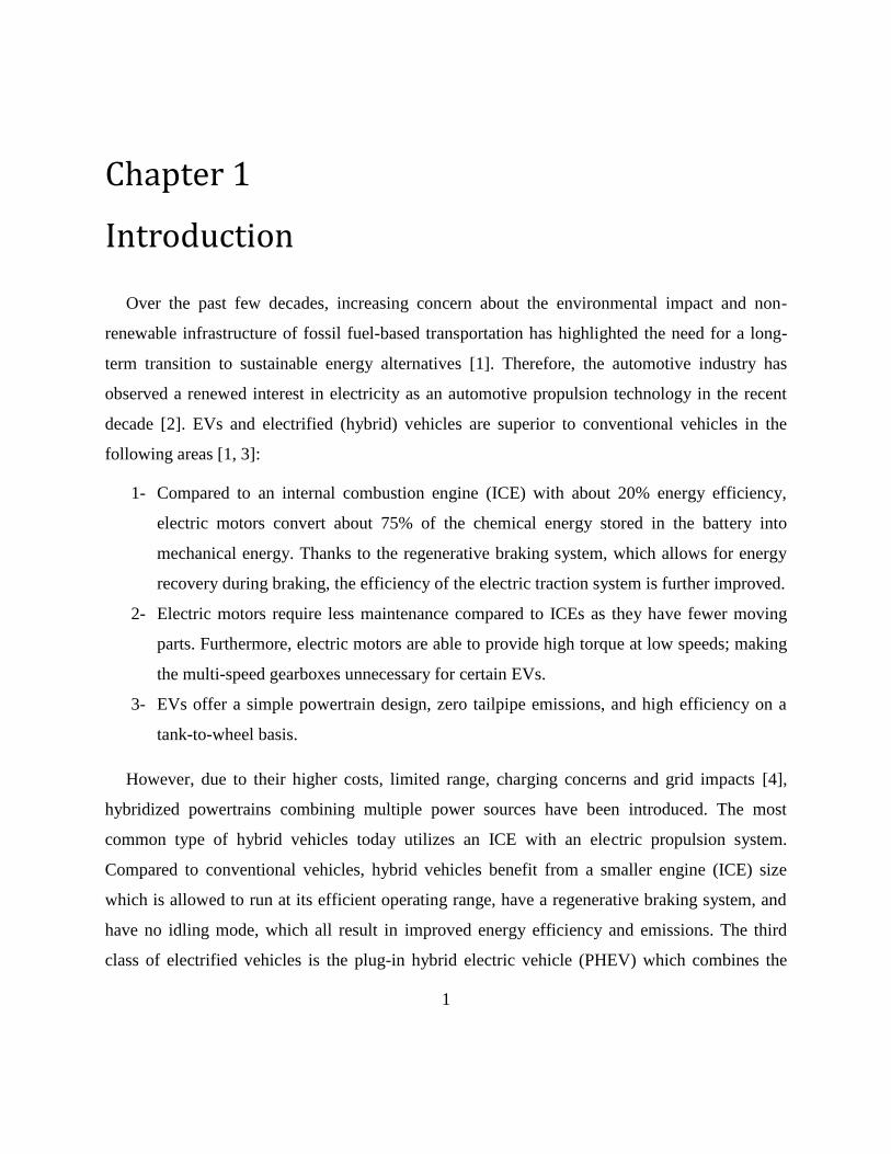
have a series, parallel or series-parallel design. In a series design, the traction power is provided
to the wheels by the battery through the electric motor and the ICE charges the battery (through a
generator) to maintain the battery state of charge (SOC) within a specified range. The power
flow in a series design is shown in Figure1-1.
Figure1-1. Power flow in a series HEV powertrain [5]
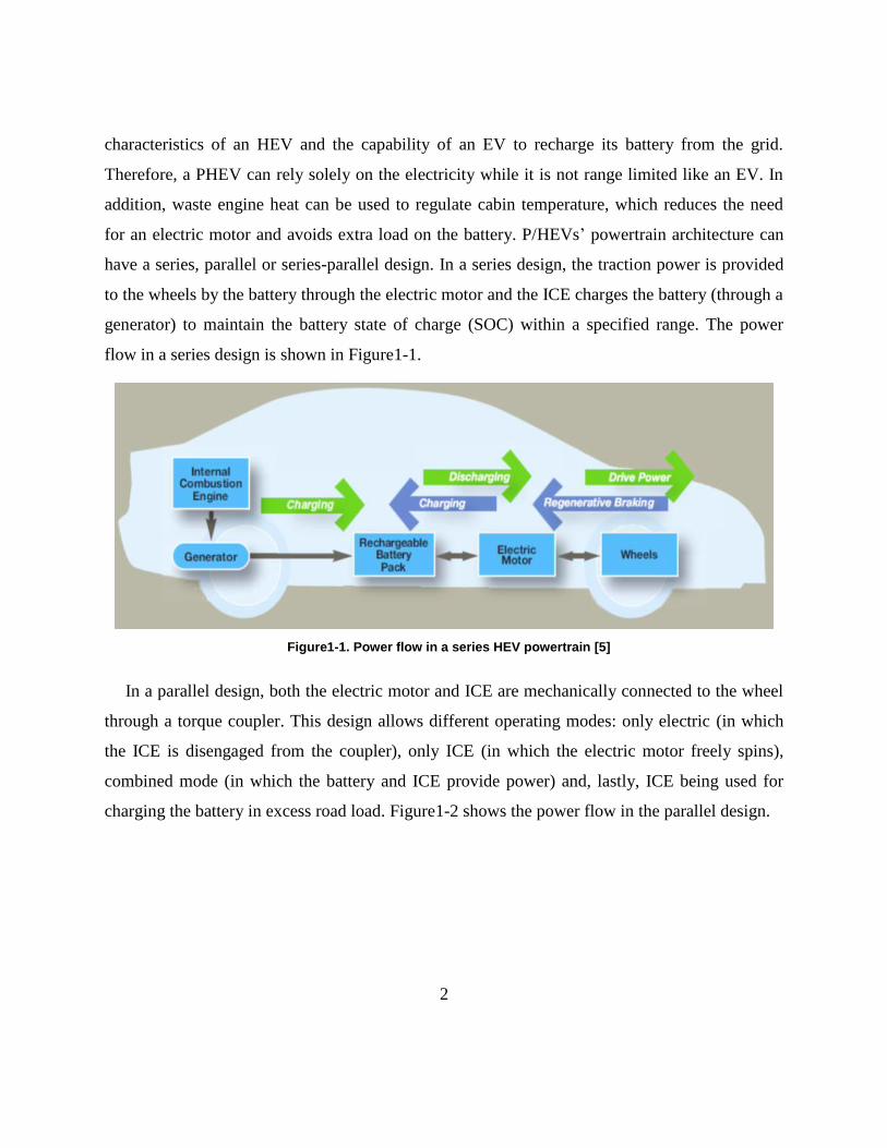
In a parallel design, both the electric motor and ICE are mechanically connected to the wheel
through a torque coupler. This design allows different operating modes: only electric (in which
the ICE is disengaged from the coupler), only ICE (in which the electric motor freely spins),
combined mode (in which the battery and ICE provide power) and, lastly, ICE being used for
charging the battery in excess road load. Figure1-2 shows the power flow in the parallel design.
3
Figure1-2. Power flow in a parallel HEV powertrain [5]
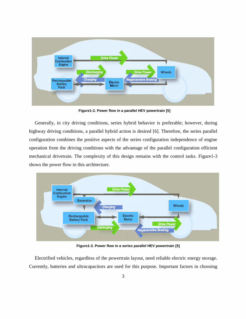
Generally, in city driving conditions, series hybrid behavior is preferable; however, during
highway driving conditions, a parallel hybrid action is desired [6]. Therefore, the series parallel
configuration combines the positive aspects of the series configuration independence of engine
operation from the driving conditions with the advantage of the parallel configuration efficient
mechanical drivetrain. The complexity of this design remains with the control tasks. Figure1-3
shows the power flow in this architecture.
Figure1-3. Power flow in a series parallel HEV powertrain [5]
Electrified vehicles, regardless of the powertrain layout, need reliable electric energy storage.
Currently, batteries and ultracapacitors are used for this purpose. Important factors in choosing
4
appropriate energy storage systems are energy and power density, lifetime and cost. Unlike
conventional vehicles in which the battery is used only for starting, ignition and lighting, in
electrified vehicles, the battery must meet certain design requirements. For example, in HEVs,
the battery is designed to operate mostly in a narrow state of charge (SOC) range which is called
charge sustaining (CS) mode and it is designed to match the peak power from the engine during
acceleration. On the other hand, in PHEVs and pure EVs, the battery is designed to provide the
vehicle with a significant all-electric range (AER) while operating in charge depleting (CD)
mode. In addition, in these vehicles, the battery experiences deep charge and discharge cycles
which adversely affect its lifetime. Therefore, the energy requirement and cycle life of a battery
in these vehicles is a crucial consideration [1]. Ultra capacitors, unlike the batteries, store electric
energy physically but not chemically; as well, they exhibit much higher power density and cycle
life but much lower energy density. Therefore, they have been mostly utilized in mild hybrid
vehicles in which the prime energy source is an engine or fuel cell [7, 8]. There is a variety of
battery technology and chemistry available today. In earlier generations, nickel cadmium, lead
acid, and nickel-metal hydride (Ni-MH) batteries were used as the power source due to their low
price and reasonable energy density [9]. In recent years, Li-ion batteries are becoming more
common because of their higher energy and power content. Li-ion battery technology is one of
the core topics in the development of PHEVs and there is plenty of ongoing research to improve
its performance, durability and safety [1, 3].
1.1 Problem definition and research objectives
In this thesis, different aspects of Li-ion battery performance and behavior are studied as
presented in the following sections.
1.1.1 Battery Performance Modeling
Electrical energy storage (battery) continues to be the greatest challenge to the
commercialization of both PHEV and EV models. Beside battery price, range anxiety (fear of
getting stranded on the road due to lack of charge) is the main concern expressed by consumers

5
[10]. Range anxiety stems from the fact that the specific energy of the battery packs (~0.25
kWh/kg) compared to fossil fuel (~13 kWh/kg) is very low. Furthermore, refuelling (recharging)
stations are not widely available and the charging time is rather high (depending on the method,
full recharge times typically range from 30 minutes to almost 12 hours). With a gasoline car,
many people are not at all affected by the range they get as refuelling is quick and easily
accessible almost everywhere. Several surveys have been conducted on range anxiety. Accenture
[11] conducted a survey, in 13 countries, on consumer preference concerning driving an
electrified vehicle in which Chinese participants showed the highest tendency to buy and drive
an EV as their future choice, while Dutch participants expressed the lowest interest. However, a
higher range means a bigger battery size and, consequently, a higher cost vehicle.
A determinant factor on the EV range is the battery management system (BMS). In electrified
vehicles, the BMS plays a significant role in the battery and the whole vehicle performance,
efficiency and safety. The BMS is actually required to respond to dynamic power demands
dependent on driving behavior, road conditions, and electrical accessories [12]. In addition, the
BMS is responsible for cell safety. Therefore, accurate prediction of SOC, proper management of
current and temperature, andcell potential balance areBMS’crucial tasks [13]. However, the
efficiency of a BMS is highly dependent on the fidelity of the battery model built in the BMS.
Furthermore, on board processing power is limited. Therefore, it is imperative to have an
accurate model that is sufficiently simple to be operated on board the BMS. Model complexity is
dependent on application requirements. High fidelity Li-ion electrochemical models, which were
first introduced by Doyle et al. [14], are widely used for battery design. Another type of battery
model is the equivalent circuit model (ECM). These models are more useful for real-time
applications (such as BMSs), in which cost and processing power is strictly limited. An ECM
represents the complex electrochemical interactions within a battery as simple circuit
components. Components may be added to model observed phenomena and increase accuracy,
or may be removed to increase efficiency. ECM circuit elements, such as resistors and
capacitors, may also be scaled to account for changes in SOC [15-18], temperature [16, 19-22],
aging [23], and C-rate [18], which affect cell performance.

6
As a contribution to the existing models, this thesis presents a comprehensive ECM developed
for two commercially available Li-ion cells used in PHEVs, which, compared to commonly used
models, proves to be more efficient (up to 6%) in terms of voltage prediction. Such an
improvement in voltage prediction can be interpreted as an additional few kilometers to the
vehicle range. Also, the proposed ECM has the capability to be used as an alternative to hybrid
pulse power characterization (HPPC) tests within a limited error.
1.1.2 Battery Thermal Characterization
Devices with high energy density, such as Li-ion batteries, have the potential for high heat
generation and Li-ion batteries are no exception. A single Li-ion polymer cell can undergo a
temperature increase of 5 to 20 K at a 1C discharge rate [24], depending on cell geometry and
assembly. Thermal management of the cells in a pack is, therefore, an important issue that must
be considered to ensure vehicle safety, performance and cycle life.
Depending on ambient conditions, there may be a need to remove or add heat to the battery in
order to maintain the optimal temperature range and distribution. Non-uniform temperature
distribution results in low charge and discharge performance and cell unbalancing, over time.
Existing thermal management techniques include applying liquids, insulations and phase-change-
materials [25]. Essential tools in automotive pack design and thermal management are thermal
and performance models. Such models require inputs such as system and operational parameters.
Not all of these parameters are easy to directly quantify (e.g. heat effect and transport properties)
because their effects cannot be isolated; thus, extensive tests are necessary to yield a clear
understanding of heat generation and cell performance [26]. Several papers have been published
on this topic so far; some proposing a simple one dimensional(1-D) [21, 27] approach and others
with further details by three dimensional(3-D) [28]modeling of the heat generation inside the
cell. However, for vehicle simulation and BMS applications, a fast and accurate heat generation
model based on a limited number of lab tests may serve as an adequate alternative.
In this regard, this thesis contributes to the literature by presenting a simple and accurate
modeling approach of Li-ion cell heat generation that can be readily applied for fast simulations

7
and on-board applications.
1.1.3 Battery Degradation
Battery state of health (SOH) has been a hot topic since rechargeable (secondary) batteries
were introduced to the industry. To extend the battery lifetime, the focus has been initially on
minimizing the power consumption of the devices powered by these batteries. However, such
methods would not be adequate, as they ignore important characteristics of the battery source
such as the dependency of available capacity on the battery discharge rate and internal
temperature, and the cycle aging effect [29]. In recent years, a number of researchers have
developed models for battery SOH and degradation rate based on battery detailed
electrochemistry coupled with thermal characteristics [30, 31]. In EV applications, battery SOH
is known to be very much dependent on the driving and charging habit; therefore, there is a
growing desire to evaluate the path dependence of battery degradation. This is due to the fact that
a lab environment is far different from what the battery experiences under real operation in EVs.
However, real-life testing is expensive and labor intensive and is associated with a very low level
of control, which explains why, so far, it has rarely been the subject of research [32-34].
As a contribution to the existing literature, this research presents a field study conducted on
the Li-ion battery running in a converted EV to correlate battery degradation with real-life
driving and charging profiles.
1.1.4 Auxiliary Loads in EVs
In EVs, the on-board battery provides the power not only for driving but also auxiliary loads
such as climate control loads. Therefore, the use of a climate control system (air conditioning
(AC) & heating) adds more challenges to the EV design. The primary task of AC is to provide
passengers’thermalcomfortthroughmaintainingthevehiclecabintemperatureandhumidityat
desired levels. AC is believed to be the accessory that requires the largest quantity of power from
the traction source. In conventional and hybrid electric vehicles (HEVs), this power is provided
by the engine; however, in EVs, the power has to be extracted from the battery [35, 36]. It is
8
reported that, in an EV, AC may reduce the driving range up to 35%, depending on the AC usage
frequency [37]. The loads are more significant when the climate-control systems are used in an
initially very hot or very cold cabin at the beginning of a trip. Associated with the range
reduction, there would be increased battery degradation for the same distance driven when
AC/heating system is operating. Therefore, it is necessary to develop a tool for assessing the
climate control system impact on the battery and vehicle performance. A modeling approach will
be presented in this thesis that enables quantifying these impacts.
1.2 Document Organization
Chapter 2: presents a literature review about the fundamentals and modeling of batteries used
in electrified vehicle and plug-in hybrid vehicle general considerations.
Chapter 3: this chapter is based on the papers published and submitted by Ehsan Samadani et
al. [38, 39]. In this chapter, first, two commercially available Li-ion batteries are studied through
thermal experiments. Profiles of heat generation at different operating conditions are generated
and a data driven model for predicting the thermal ramp rate is developed. Afterwards, results of
EIS tests conducted on the two cells are presented and, based on the observed phenomena during
the EIS tests, an equivalent circuit model to predict the cells performance (voltage) under an
arbitrary loading profile is developed.
Chapter 4: is based on the submitted report by Ehsan Samadani et al to the Transport Canada.
[40]. In this chapter, results of field tests with a converted EV are presented through four major
steps. First, implementation of a system to collect, store, analyze, and report vehicle and grid
electricity usage data. Second, development of a powertrain model of the EV that includes
battery degradation based on the collected data. Third, a feasibility study of using the EV as a
replacement for the conventional fleet vehicles in operation by the owner company. Fourth,
study of the battery degradation through collected data over the course vehicle operation. The
study focus is to identify the degradation trends in the battery and propose a pathway for
degradation modeling.

9
Chapter 5: presents a vehicle life time modeling considering temperature profiles, powertrain
architectures, drive cycles and battery conditioning impacts. For this purpose, a thermal model
of the vehicle cabin is developed. This model is able to predict the cabin temperature profile
given a certain ambient and initial condition. The model is integrated to the battery model to
determine the extra load on the battery and resulting extra capacity loss.
Chapter 6: This chapter summarizes the thesis, and highlights the main contributions of the
research. It also contains recommendations for future works.

10
Chapter 2
Background and literature review
In this chapter, related background and literature on the battery modeling is presented.
2.1 Battery Elements and Specifications
Battery is an energy storage device consisting of one or more electrochemical cells that
produces electrical energy from chemical energy stored in its active materials through
electrochemical reactions. Depending on the desired nominal battery voltage and capacity Cells,
are connected in series, parallel or both. Main components of a cell are anode, cathode and
separator.
2.1.1 Anode
Upon the chemical reaction at the anode (oxidation) electrons are released and flow to the
cathode through an external circuit. Important parameters in selecting the anode material are
efficiency, high specific capacity, conductivity, stability, ease of fabrication and low cost.
2.1.2 Cathode
Cathode is the electrode in which reduction (absorbing electrons) takes place. During
discharge the positive electrode of the cell is the cathode. During charge the situation reverses
and the negative electrode of the cell is the cathode. The cathode is selected based on its voltage
and chemical stability over time.
2.1.3 Electrolyte
Substances that release ions when dissolved in water are called electrolytes; which could
include a wide range of acids, bases, and salts, as they all give ions when dissolved in water. The
electrolyte completes the cell circuit by transporting the ions. The electrolyte are desired to be

11
highly conductive, non-reactive (with the electrode materials), stabile in properties at various
temperatures, and economical.
2.1.4 Separator
A separator is a porous membrane inserted between electrodes of opposite charge. The key
function of the separator is to keep the positive and negative electrodes apart to prevent electrical
short circuits and, at the same time allow rapid transport of ionic charge carriers needed to
complete the circuit. Care must be taken upon selecting the separator material, as it could
adversely affect the battery performance (by increasing electrical resistance). Following
considerations should be observed when selecting the separator [41]:
Electrical insulation
Minimal electrolyte (ionic) resistance
Mechanical stability
Chemical resistance to degradation by electrolyte
Uniform in property and thickness
Effective in preventing migration of particles
2.2 Battery Gloassary
2.2.1 Battery Management System
Battery management unit (BMU) is the central component of the battery system to ensure a
healthy and appropriate usage of the sensitive battery cells. The BMU controls the usage of the
battery cells by measuring variables such as voltage, current and temperature of each individual
cell in the package. It also calculates important state variables such as SOC and power limits for
charge and discharge of the battery. This information along with other signals (such as alarm
signals) is sent from the BMU to the vehicles main computer which consequently is able to

12
control the propulsion of the vehicle in a qualitative manner without damaging the battery
package [3].
2.2.2 State of Charge
The state of charge (SOC) indicates the amount of charge in Amp-hours left in the battery.
The SOC can be divided into two types: engineering-SOC (e-SOC) and thermodynamic SOC (t-
SOC) [42]. The e-SOC is the SOC apparent to the user of the battery and is rate dependent; it is
the state of the capacity at a certain discharge rate, so different discharge rates will result in a
different e-SOC at the same amount of charge in the battery. The t-SOC is the SOC of a battery
defined by the thermodynamic properties in the cell and can be determined by the open circuit
voltage of the battery; it is the state of the useable capacity in the cell.
2.2.3 Depth of Discharge-
A measure of how much energy has been withdrawn from a battery, expressed as a percentage
of full capacity. For example, a 100 Ah battery from which 30 Ah has been withdrawn has
undergone a 30% depth of discharge (DOD). Depth of discharge is the inverse of state of charge.
2.2.4 C-rate
The C-rate is a measure for the current of a battery cell and is scaled to the nominal capacity
of a cell stated by the manufacturer at reference conditions. The current level that a battery cell
can discharge at depends on the capacity of the battery. A current of 1C means that the battery
cell is ideally charged or discharged in one hour, C/2 in two hours and 2C in half an hour. So a
current of 0.5C for a cell with nominal capacity of 160Ah is equal to 80A.
2.2.5 Cell Capacity
The useable capacity is theoretically the possible amount of charge that can be discharged
from a fully charged cell with an infinitely small current for a given minimum cell voltage, so
that the voltage drop over the internal resistance becomes close to zero. The true capacity is the
useable capacity under reference temperature and is used as a measure for the capacity fading

13
determination. The 1C capacity is determined with a C-rate of 1C under reference conditions and
is generally used to measure the capacity fading [43].
2.2.6 Cycle
Cycle could be defined as a period of discharge followed by a full recharge. EVs, however,
experience regenerative braking during operation, which required a change in cycle definition.
Some define a cycle as a period of discharge with regenerative braking followed by a full
recharge [44] or an amount of energy discharged with regenerative braking followed by the equal
amount recharged [43]. A better alternative to measure the usage of a battery is the charge or
energy processed in the battery. The ambiguous definition of a cycle is hereby also avoided.
2.2.7 Cell Open Circuit Voltage
By definition, the open-circuit voltage (OCV) is the battery voltage under the equilibrium
conditions, i.e. the voltage when no current is flowing in or out of the battery, and, hence no
reactions occur inside the battery. OCV is a function of State-of-Charge and is expected to
remain the same during the life-time of the battery. Note, however, that other battery
characteristics do change with time, e.g. capacity is gradually decreasing as a function of the
number of charge-discharge cycles.
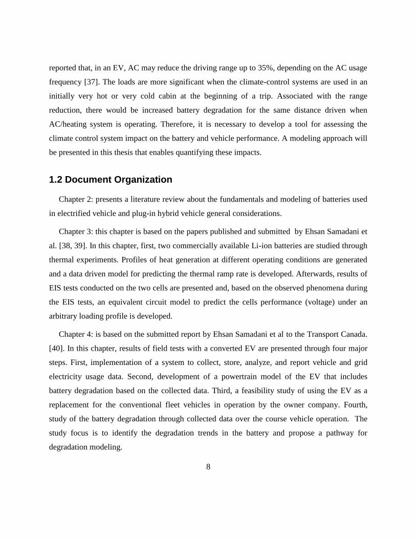
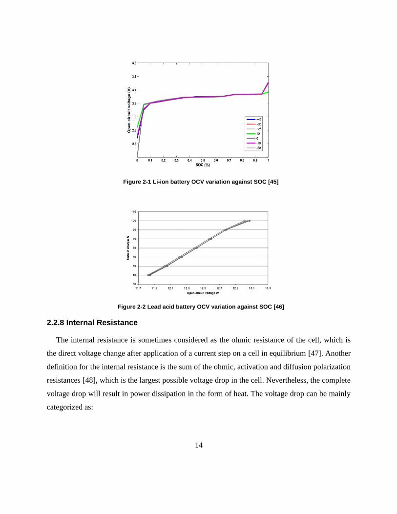
Because open circuit voltage shows a strong dependence on SOC for most batteries, it can be
used as an estimation method. Because the battery must be at rest (several hours) for an OCV to
be determined, it is not practical for real-time or continuous estimation. This poses problems for
monitoring devices (e.g. clocks) where rest state is never realized. Additionally, Li-ion batteries
(such as those used in vehicle applications) have traditionally shown a “flat” OCV when
compared with lead acid batteries which can lead to difficulty in estimation as demonstrated in
Figure 2-1and Figure 2-2.
14
Figure 2-1 Li-ion battery OCV variation against SOC [45]
Figure 2-2 Lead acid battery OCV variation against SOC [46]
2.2.8 Internal Resistance
The internal resistance is sometimes considered as the ohmic resistance of the cell, which is
the direct voltage change after application of a current step on a cell in equilibrium [47]. Another
definition for the internal resistance is the sum of the ohmic, activation and diffusion polarization
resistances [48], which is the largest possible voltage drop in the cell. Nevertheless, the complete
voltage drop will result in power dissipation in the form of heat. The voltage drop can be mainly
categorized as:
15
IR drop
IR drop or ohmic drop is due to the current flowing across the internal resistance of the
battery.
Activation polarization
Activation polarization refers to the various retarding factors inherent to the kinetics of an
electrochemical reaction, like the work function that ions must overcome at the junction between
the electrodes and the electrolyte.
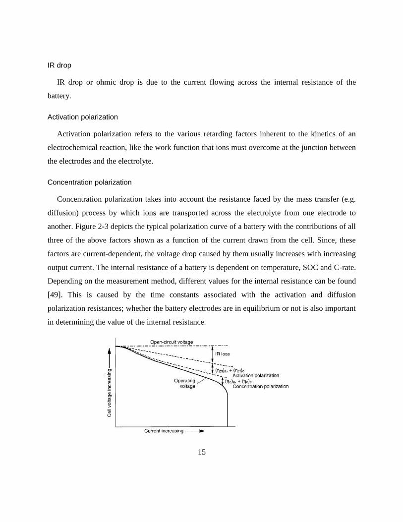
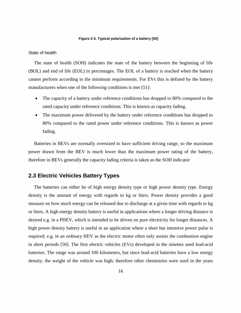
Concentration polarization
Concentration polarization takes into account the resistance faced by the mass transfer (e.g.
diffusion) process by which ions are transported across the electrolyte from one electrode to
another. Figure 2-3 depicts the typical polarization curve of a battery with the contributions of all
three of the above factors shown as a function of the current drawn from the cell. Since, these
factors are current-dependent, the voltage drop caused by them usually increases with increasing
output current. The internal resistance of a battery is dependent on temperature, SOC and C-rate.
Depending on the measurement method, different values for the internal resistance can be found
[49]. This is caused by the time constants associated with the activation and diffusion
polarization resistances; whether the battery electrodes are in equilibrium or not is also important
in determining the value of the internal resistance.
16
Figure 2-3. Typical polarization of a battery [50]
State of health
The state of health (SOH) indicates the state of the battery between the beginning of life
(BOL) and end of life (EOL) in percentages. The EOL of a battery is reached when the battery
cannot perform according to the minimum requirements. For EVs this is defined by the battery
manufacturers when one of the following conditions is met [51]:
The capacity of a battery under reference conditions has dropped to 80% compared to the
rated capacity under reference conditions. This is known as capacity fading.
The maximum power delivered by the battery under reference conditions has dropped to
80% compared to the rated power under reference conditions. This is known as power
fading.
Batteries in BEVs are normally oversized to have sufficient driving range, so the maximum
power drawn from the BEV is much lower than the maximum power rating of the battery,
therefore in BEVs generally the capacity fading criteria is taken as the SOH indicator
2.3 Electric Vehicles Battery Types
The batteries can either be of high energy density type or high power density type. Energy
density is the amount of energy with regards to kg or liters. Power density provides a good
measure on how much energy can be released due to discharge at a given time with regards to kg
or liters. A high energy density battery is useful in applications where a longer driving distance is
desired e.g. in a PHEV, which is intended to be driven on pure electricity for longer distances. A
high power density battery is useful in an application where a short but intensive power pulse is
required; e.g. in an ordinary HEV as the electric motor often only assists the combustion engine
in short periods [50]. The first electric vehicles (EVs) developed in the nineties used lead-acid
batteries. The range was around 100 kilometers, but since lead-acid batteries have a low energy
density, the weight of the vehicle was high; therefore other chemistries were used in the years
17
after [52]. Due to the higher power and energy density and improved cycle life, EVs started to
use nickel metal hydrate (NiMH).Today NiMH batteries are still used in hybrid electric vehicles
(HEV) and plug-in hybrid electric vehicles (PHEV) for their low cost per Watt. But, due to high
self-discharge, limited SOC operation range and low energy density, these batteries are
unsuitable for EVs. ZEBRA or molten salt batteries are also used in EVs. These batteries have a
low cost and high safety, but because of high operating temperature (270-350˚C)andlowpower
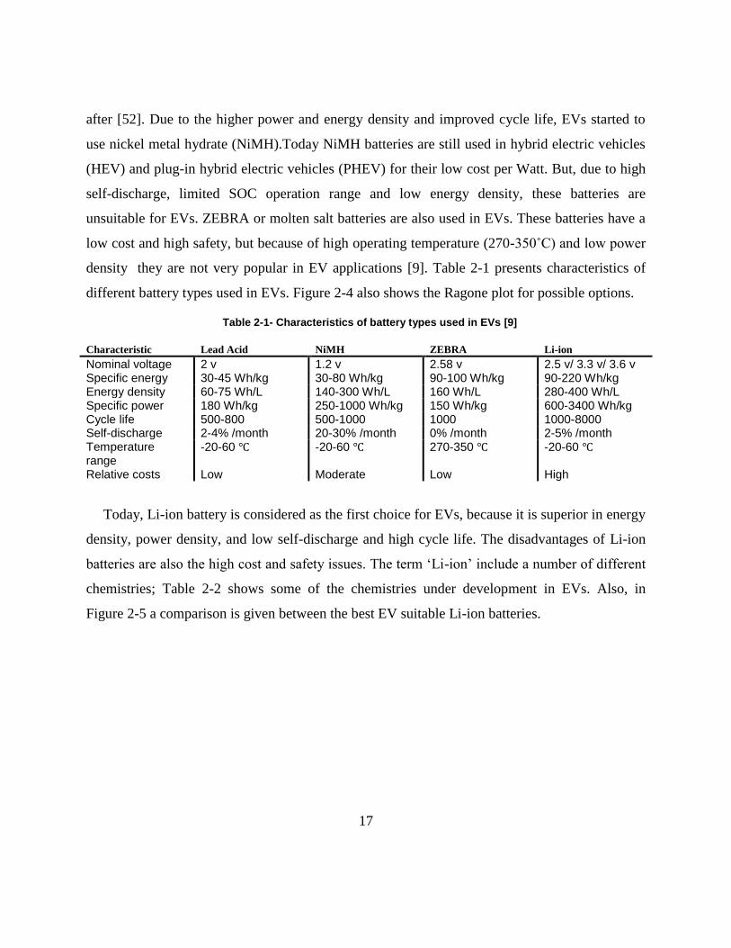
density they are not very popular in EV applications [9]. Table 2-1 presents characteristics of
different battery types used in EVs. Figure 2-4 also shows the Ragone plot for possible options.
Table 2-1- Characteristics of battery types used in EVs [9]
Characteristic Lead Acid NiMH ZEBRA Li-ion
Nominal voltage 2 v 1.2 v 2.58 v 2.5 v/ 3.3 v/ 3.6 v Specific energy 30-45 Wh/kg 30-80 Wh/kg 90-100 Wh/kg 90-220 Wh/kg Energy density 60-75 Wh/L 140-300 Wh/L 160 Wh/L 280-400 Wh/L Specific power 180 Wh/kg 250-1000 Wh/kg 150 Wh/kg 600-3400 Wh/kg Cycle life 500-800 500-1000 1000 1000-8000 Self-discharge 2-4% /month 20-30% /month 0% /month 2-5% /month Temperature range
-20-60 ℃ -20-60 ℃ 270-350 ℃ -20-60 ℃
Relative costs Low Moderate Low High
Today, Li-ion battery is considered as the first choice for EVs, because it is superior in energy
density, power density, and low self-discharge and high cycle life. The disadvantages of Li-ion
batteriesarealsothehighcostandsafetyissues.Theterm‘Li-ion’includeanumberofdifferent
chemistries; Table 2-2 shows some of the chemistries under development in EVs. Also, in
Figure 2-5 a comparison is given between the best EV suitable Li-ion batteries.

18
Figure 2-4. The Ragone plot of various cell types capable of meeting the requirements for EV applications
[53] .
As an example, Lithium-iron-phosphate (LiFePO4/LFP) does not experience thermal runaway
and has almost no fire hazards, since no oxygen is released at high temperatures [54]. LiFePO4
cells have the lowest costs per Ah and kW [54, 55], good life span, good power capabilities and
are extremely safe, but they have low specific energy and poor performance at low temperatures.
Table 2-2- Examples of different Li-ion batteries used in EVs [4]
Developer Chemistry Vehicle Year
A123 Doped Lithium nanophosphate
Fisker-Karma Vue-PHEV Think
2010 2009 2009 Panasonic
JCI-Saft Lithium nickel cobalt Aluminum oxide
Toyota-PHEV S400-HEV Vue-PHEV
2010 2009 2009 Hitachi Lithium cobalt oxide GM-HEV 2010
Altair Nanotechnologies Lithium titanate spinel Phoenix Electric
2008
EnerDel Lithium manganese Titanate
Think 2009
Compact (LG) NEC
Manganese spinel Volt-EV Nissan-EV
2010 2010

19
Figure 2-5. Comparison of suitable Li-ions for EV. The more the colored shape extends along a given
axis, the better the performance in that direction [56].
2.4 Li-ion Cell Operation
A battery cell converts chemical energy to electrical energy. This is done by oxidation at one
electrode and reduction at the other electrode. Li-ion battery cells utilize lithium ions to store and
provide energy. A Li‐ion battery cell consists of two electrodes, cathode and anode, with a
separator in between, and current collectors on each side of the electrodes. The anode is usually
made out of graphite or a metal oxide. The cathode is made of a composite material and defines
the name of the Li-ion battery cell. The electrolyte can be liquid, polymer or solid. The separator
is porous to enable the transport of lithium ions. It prevents the cell from short‐circuiting and
thermal runaway [57]. During discharge the lithium ions diffuse from the anode to the cathode
through the electrolyte. The lithium ions will intercalate into the cathode, causing the cathode to
become more positive. Due to the potential difference between the cathode and anode, an electric
current will flow through the external circuit, supplying power to the load. During charging the
opposite effect occurs. The current will cause the lithium ions to deintercalate from cathode and
diffuse to the anode. At the anode intercalation of the lithium ions occur, charging the battery.
These processes are shown in Figure 2-6 for a Li-ion cell.

20
Figure 2-6.Charge and discharge process in Li-ion battery [58]
Li-ion cells are manufactured in various types of cell formats and geometries. Some of them
are illustrated in Figure 2-7.
Cylindrical [56]
Prismatic [56]
Pouch [56] Figure 2-7 Types of Li-ion cell formats: cylindrical, prismatic and pouch cell.

21
2.5 Battery Models
A major obstacle in PHEV commercialization is the high cost of the battery pack. To address
this issue, different solutions such as energy density improvements, reduction of material cost,
etc. could be considered. To come up with an optimal solution, one approach is to develop
battery models. Battery modeling, in fact, provides information on battery charging/discharging
and transient behavior and health status of the battery (battery degradation) as a function of
different stress factors (temperature, discharge rate, etc.). EV designer use battery models for
sizing the required battery and predict the battery performance. Battery models are also used for
on-line self-learning performance and SOC estimation in BMS [59-61]. Common battery models
used in the automotive applications are reviewed in the following sections.
2.5.1 Electrochemical Models
Battery modeling based on electrochemical equations provides a deep understanding of the
physical and chemical process inside the battery and makes it useful when designing a cell, but
high computational time makes these models improper for applications with high dynamics. The
first electrochemical modeling approach to porous electrodes with battery applications was
presented by Newman and Tiedemann in 1975 [62]. In the porous electrode theory, the electrode
is treated as a superposition between the electrolytic solution and solid matrix, the matrix itself is
modeled as microscopic spherical particles where lithium ions diffuse and react on the sphere
surface. This approach was expanded to include two composite models and a separator by Fuller
et al. in 1994 [63]. This model was later adapted for Ni-MH batteries [64], and then Li-ion
batteries [27].
2.5.2 Equivalent Circuit Models
Equivalent circuit-based modeling (ECM) is suitable for automotive real time applications
(such as BMS design), since it does not need deep understanding of electrochemistry of the cell
22
and at the same time it is well capable of simulating the battery dynamics. ECMs simulate the
battery as a circuit often composed of resistors, capacitors, and other elements. There is a wide
selection of models depending with tradeoffs of accuracy and time required. A large capacitor or
ideal voltage source is selected to represent the open-circuit voltage (OCV), with the remainder
of the circuit representing battery internal resistance and dynamic effects (e.g. terminal voltage
relaxation). Generally, each observed phenomena is modeled with an individual circuit
component. For example, the bulk electrolyte resistance is represented with a simple resistor, R0.
To keep the model simple, similar phenomena (e.g. concentration and electrochemical
polarization effects) could be grouped, although this decreases model accuracy. Resistances of
other components such as electrodes and separator are additive, and included in R0. Other
phenomena including the polarization effect of the battery are usually represented by capacitors
and resistors in parallel. In addition, diffusion effects are represented by a Warburg element. In
the following, common ECMs used in PHEV applications are presented.
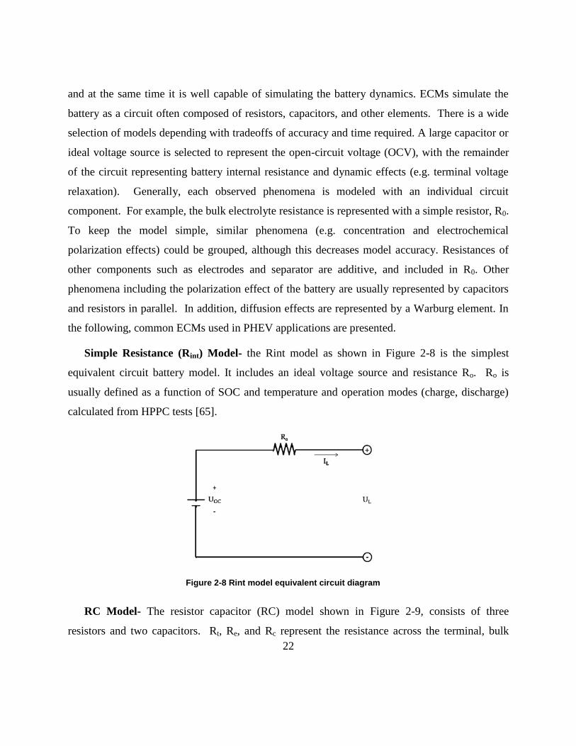
Simple Resistance (Rint) Model- the Rint model as shown in Figure 2-8 is the simplest
equivalent circuit battery model. It includes an ideal voltage source and resistance Ro. Ro is
usually defined as a function of SOC and temperature and operation modes (charge, discharge)
calculated from HPPC tests [65].
Figure 2-8 Rint model equivalent circuit diagram
RC Model- The resistor capacitor (RC) model shown in Figure 2-9, consists of three
resistors and two capacitors. Rt, Re, and Rc represent the resistance across the terminal, bulk

23
solution, and surface respectively. Cb representsthebattery’sabilitytochemicallystorecharge.
Cc, which has a small value, represents battery surface effects [65].
Figure 2-9 RC model equivalent circuit diagram
Thevenin Model- Thevenin Model circuit structure is shown in Figure 2-10. E0 describes the
battery’s open circuit voltage. R0 describes battery’s internal resistance. I (t) is the battery’s
charge or discharge currentandU(t)isthebattery’sterminalvoltage.TheRCcircuitdescribes
the battery polarization [66].
Figure 2-10 Thevenin model equivalent circuit diagram [66]
DP Model- Although a single RC component is capable of modeling polarization (like
Thevenin), but, it becomes less accurate at the end of charge or discharge. The DP model shown
in Figure 2-11 improves the polarization characteristics by simulating the concentration and
electrochemical polarization effects separately. Rpa and Rpc represent electrochemical and
24
concentration polarization respectively. Cpa and Cpc characterize the transient response during
power transfer for electrochemical and concentration polarization respectively [65].
Figure 2-11 DP model equivalent circuit diagram [65].
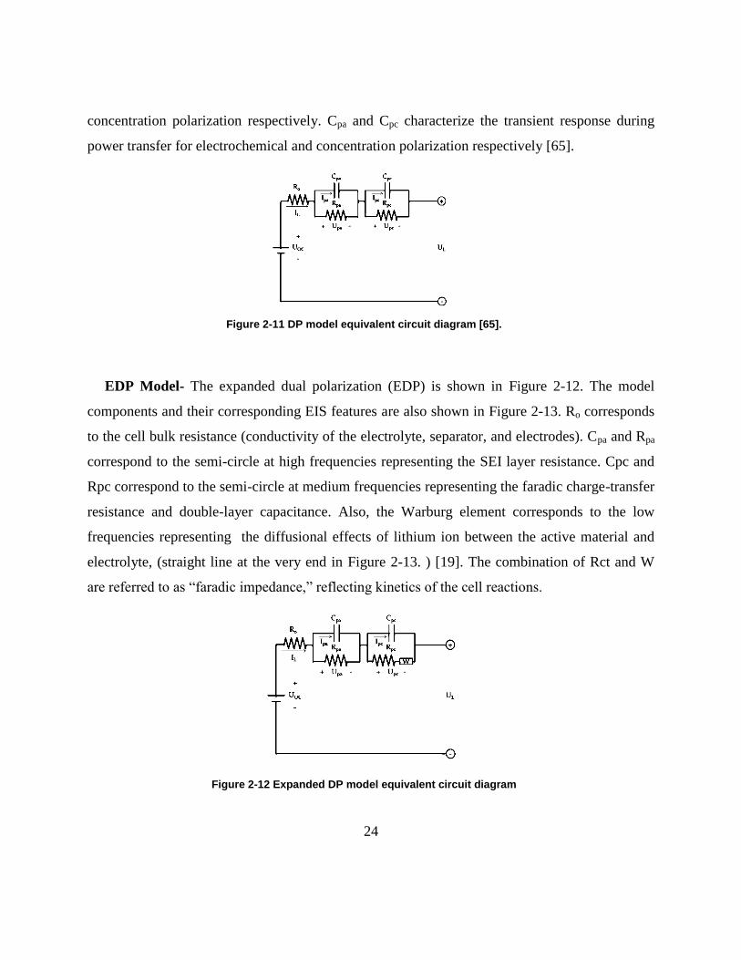
EDP Model- The expanded dual polarization (EDP) is shown in Figure 2-12. The model
components and their corresponding EIS features are also shown in Figure 2-13. Ro corresponds
to the cell bulk resistance (conductivity of the electrolyte, separator, and electrodes). Cpa and Rpa
correspond to the semi-circle at high frequencies representing the SEI layer resistance. Cpc and
Rpc correspond to the semi-circle at medium frequencies representing the faradic charge-transfer
resistance and double-layer capacitance. Also, the Warburg element corresponds to the low
frequencies representing the diffusional effects of lithium ion between the active material and
electrolyte, (straight line at the very end in Figure 2-13. ) [19]. The combination of Rct and W
arereferredtoas“faradicimpedance,”reflectingkineticsofthecellreactions.
Figure 2-12 Expanded DP model equivalent circuit diagram

25
Figure 2-13 EDP model components correlated with EIS results [19]
2.6 Battery Degradation Modeling
Modeling of degradation is mainly based on the aging experiments and measurements and the
complexity of the model depends on the number of stress factors and degradation mechanisms to
be incorporated in the modeling. It is worth to mention that each battery type experiences a
specific degradation mechanism and not all stress factors have similar impact on different battery
chemistries.
To date, assessment and understanding of battery performance in EVs primarily relies on lab
testing. Similar to standard driving schedule tests and analyses, these tests and duty cycle
analyses have constraints in their validity to real-life operation. A main issue in both cases is that
even under specific driving cycles or duty cycles; energy consumption strongly depends on
uncontrolled ambient operating conditions. On the other hand, conducting drive cycle analysis
using trip data collected from real-life vehicle operation is a challenging task [67]. Although
quite helpful in evaluating battery state of health (SOH), very limited effort has been put into
field testing with detailed data collection and analysis, mainly because such testing is costly and
virtually no control[32].

26
2.7 Degradation Mechanisms of Li-ion Cells
The other aspect of batteries as traction sources is the battery durability and life which is of
much concern in PHEVs. As the battery ages, it becomes less able to store and supply energy.
Theformerisknownas“capacityfade”andthelatteras“powerfade”.Knowledgeaboutbattery
durability is also of much importance from the customer point of view, i.e. knowing how far the
battery will operate properly over a reasonable period without needing a replacement and
additional costs. Of course, it strongly depends on the operating conditions and the environment
that the battery is exposed to.
In PHEV applications, the battery lifetime by convention is defined as the time period that the
battery loses 20% of its initial capacity [66]. Batteries are designed for 8-10 years of service.
However, battery lifetime is affected by several factors. High power imposed on the battery
during acceleration and braking, which could be up to ten times higher than the average power
demand, as well as driving behavior, extreme ambient temperature and charging habit all are
known to be significant factors on the battery state of health (SOH). To improve the battery
performance and lifetime prediction models these effects should be carefully taken into account
[67]. Also thermal heating of the cell can significantly reduce the lifetime of a battery.
Li-ion cells undergo degradation in terms of capacity and power capability as result of
continuous usage and also during the storage time. The performance degradation during cycling
occurs much faster than storage under the same conditions. In the following, normal and
accelerated degradation mechanisms for cycling and storage will be described.
2.7.1 Degradation under Storage (i.e. Calendar Aging)
Even under storage status, the active anode material is exposed to the electrolyte through the
porous SEI layer, and side reactions enhance this SEI layer. High SOCs or high temperatures
result in more severe capacity fading and resistance growth (power fading) in the cell as well.
Therefore, to slow down the electrochemical processes and improve battery life, Li-ion cells
need to be stored under optimal conditions (40% SOC and 15°C [68]).
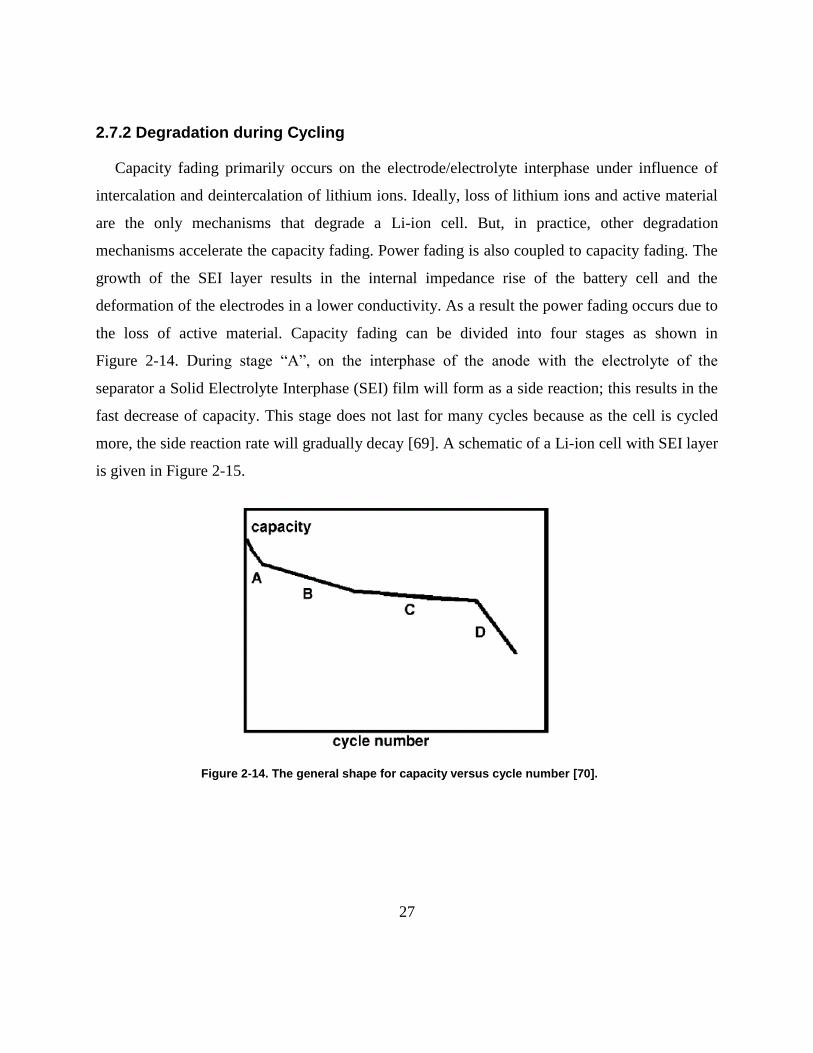
27
2.7.2 Degradation during Cycling
Capacity fading primarily occurs on the electrode/electrolyte interphase under influence of
intercalation and deintercalation of lithium ions. Ideally, loss of lithium ions and active material
are the only mechanisms that degrade a Li-ion cell. But, in practice, other degradation
mechanisms accelerate the capacity fading. Power fading is also coupled to capacity fading. The
growth of the SEI layer results in the internal impedance rise of the battery cell and the
deformation of the electrodes in a lower conductivity. As a result the power fading occurs due to
the loss of active material. Capacity fading can be divided into four stages as shown in
Figure 2-14. During stage “A”, on the interphase of the anode with the electrolyte of the
separator a Solid Electrolyte Interphase (SEI) film will form as a side reaction; this results in the
fast decrease of capacity. This stage does not last for many cycles because as the cell is cycled
more, the side reaction rate will gradually decay [69]. A schematic of a Li-ion cell with SEI layer
is given in Figure 2-15.
Figure 2-14. The general shape for capacity versus cycle number [70].

28
Figure 2-15.Schematic of SEI film layer in Li-ion battery [71]
In the stage B, anode is the limiting electrode [69]. Due to the SEI film layer formed on the
anode, less active material is available and less lithium ions are intercalated into the anode during
charging. As a result the loss rate of lithium ions will be slower, and the SEI layer protects the
anode from reduction reactions with the electrolyte. During continuous intercalation and
deintercalation the SEI layer cracks and more active material will be exposed. This will cause
more side reactions and the SEI layer will continue to grow, leading to a less porous SEI layer
and loss of lithium ions.
In stage C, the degradation rate of the active cathode material is higher than the loss of lithium
ions. On the cathode/electrolyte interphase layer similar to the SEI layer is formed, which is
named the Solid Permeable Interphase (SPI) [72]. This layer will also grow due to cycling and
limit the active cathode material. The anode is however still the limiting electrode in this stage,
as there is still more active cathode material available than lithium ions.
In stage D, due to the high degradation rate of the cathode, the cathode becomes the limiting
electrode.Lessactivecathodematerialisavailablethantheamountof‘cycleable’lithiumions
[69]. Not all the lithium ions that were intercalated into the anode during charging can be
intercalated into the cathode during discharge. Hence, more and more lithium ions are stuck
inside the anode. The cathode will be fully intercalated during discharge, which raises the active
29
cathode material loss rate. These added effects cause an accelerated capacity fading and the
capacity will rapidly decrease.
The severity of these stages is not the same for different types of Li-ion cells. For example,
for LiFePO4, the main capacity fading mechanism cells is the loss of lithium ions by the lithium
ion consuming SEI film later formation, which also results in a loss of active anode material
[44]. Loss of cathode material happens at a lower rate for LiFePO4 cells, since neither cycling
nor temperature change enhances the formation of the SPI layer [72]. This causes LiFePO4 cells
to have a much higher cycling life compared to other chemistries.
2.8 Accelerated Degradation during Cycling
Stress factors like extreme temperatures, large C-rates and high SOC have negative impact on
the cell capacity and cause accelerated degradation. In the following each of these stress factors
will be described.
Depth of Discharge- The cycle life of a cell is strongly dependent on the DOD. Figure 2-16
shows typical curve of cycle number against the DOD. The deeper the discharge, the more
intercalation and deintercalation takes place in the electrodes. The loss of lithium ions and active
electrode material is higher for larger DOD cycles. At high DODs, additional degradation
mechanisms can occur resulting in decomposition and dissolution of cathode material and
capacity fading [73]. DOD has no influence on the capacity fading of LiFePO4 cells, but the
charge or energy processed is the determining factor [74].
C-rate- High currents generate more heat and cause the temperature of the cell to rise invoking
the high temperature degradation mechanisms. High currents also cause local over potential of
the electrodes; it means that the maximum voltage for the cell is reached at an earlier stage at
certain areas of the cell. High C-rates will also cause the SEI layer on the anode to crack faster.
More active anode material is exposed and the SEI layer will restore itself, reducing lithium ions
from the battery cell process. High C-rates will furthermore cause additional strain on the

30
electrode materials, resulting in increased deformation and loss of active material [73]. These
effects will all result in capacity and power fading.
Figure 2-16. Cycle life vs. ΔDoD curve for different battery cell chemistries[75]
Temperature- Li-ion cells have an optimal temperature operating range (Figure 2-17);
outside this range the battery cell undergoes severe loss of capacity. High and low temperatures
have different effect on the battery life.
Figure 2-17. Example-Battery cell’s temperature range for optimal cycle life [76]
At low temperature, due to the higher activation energy needed for the chemical reactions
and lower ion diffusion; there will be a loss of capacity and deliverable power. However, when
the temperature is restored to nominal level, the capacity and power capabilities will be
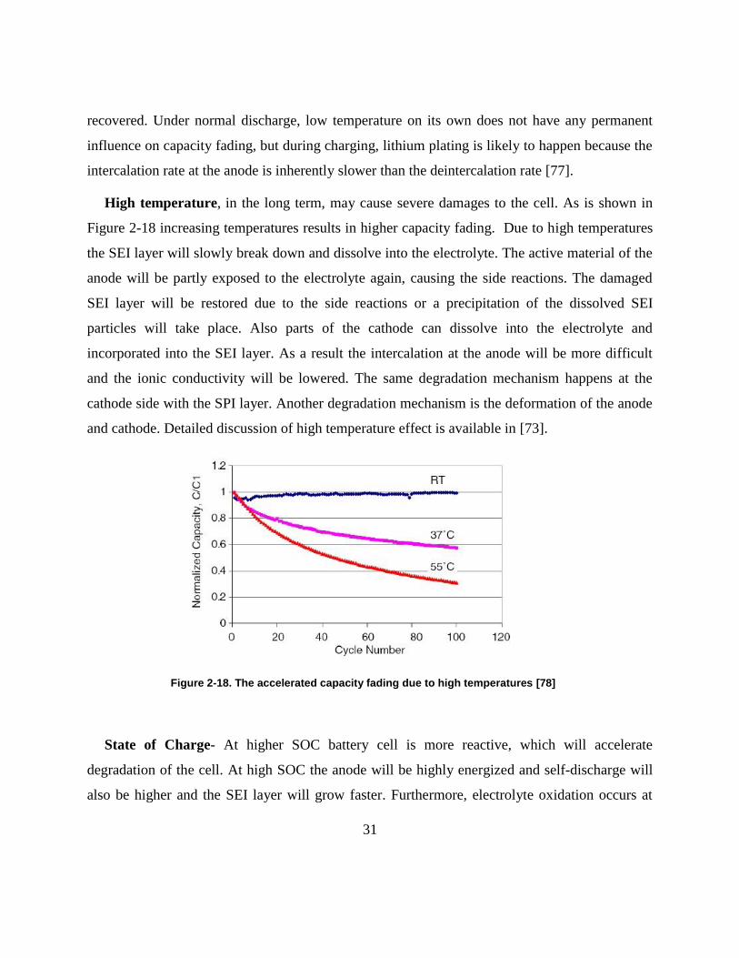
31
recovered. Under normal discharge, low temperature on its own does not have any permanent
influence on capacity fading, but during charging, lithium plating is likely to happen because the
intercalation rate at the anode is inherently slower than the deintercalation rate [77].
High temperature, in the long term, may cause severe damages to the cell. As is shown in
Figure 2-18 increasing temperatures results in higher capacity fading. Due to high temperatures
the SEI layer will slowly break down and dissolve into the electrolyte. The active material of the
anode will be partly exposed to the electrolyte again, causing the side reactions. The damaged
SEI layer will be restored due to the side reactions or a precipitation of the dissolved SEI
particles will take place. Also parts of the cathode can dissolve into the electrolyte and
incorporated into the SEI layer. As a result the intercalation at the anode will be more difficult
and the ionic conductivity will be lowered. The same degradation mechanism happens at the
cathode side with the SPI layer. Another degradation mechanism is the deformation of the anode
and cathode. Detailed discussion of high temperature effect is available in [73].
Figure 2-18. The accelerated capacity fading due to high temperatures [78]
State of Charge- At higher SOC battery cell is more reactive, which will accelerate
degradation of the cell. At high SOC the anode will be highly energized and self-discharge will
also be higher and the SEI layer will grow faster. Furthermore, electrolyte oxidation occurs at

32
high SOC, leading to impedance increase [79]. These effects result in capacity and power fading.
During storage for a long time, high SOC will have more profound effect. In case of overcharge
or over discharge, other degradation mechanisms come into play:
Overcharge- When the cell is charged over the specified voltage, a small increase in capacity
is initially obtained, but the cycle life is strongly reduced. This effect is stronger as the end of
charge voltage increases. During overcharge electrical energy is pumped into the battery, but
more intercalation can hardly take place. This will be represented by a sharp increase of internal
resistance and the temperature [51]. Decomposition of the binder and electrolyte, forming
insoluble products, blocking the pores of the electrodes, and causing gas generation subsequently
may take place [80].
Over discharge- When the cell is discharged under the specified cut-off voltage, two
degradation mechanisms severely damage the cell. 1- Corrosion of the copper current collectors
on the anode side of the cell and dissolution into the electrolyte resulting in loss of contact with
anode and power fade [81]. 2- Decomposition of the SEI layer on the anode. The high anode
potential will cause dissolution of the SEI layer. Upon recharge the exposed active material will
cause side reactions to restore the SEI layer and reducing lithium ions, causing capacity fading
[82].
2.9 Duty cycle & Drive cycle
In the analysis of the driving and charging data, terminologies such as drive cycle, duty cycle,
anddrivingpatternarefrequentlyused.A“drivecycle”referstoahistoryofdriving,typically
represented by a speedversustimecurve.A“dutycycle”referstoahistoryofpowerusageofa
device,typicallydepictedbyapowerversustimecurve.A“drivingpattern”isusedtodescribea
driving condition, taking into account both road condition (e.g., road type) and driving behavior.
Also, the duration between two successive stop is called driving pulse or micro trip which is
represented in Figure 2-19. Among popular standard drive cycles used in vehicle design and
development are, urban dynamometer driving schedule (UDDS), US06 and highway fuel

33
economy test cycle (HWFET), which represent city driving, aggressive driving (high speeds &
accelerations) and highway driving respectively [81].
Figure 2-19- Schematic of a driving cycle broken down into a series of sequential isolated “driving pulses” or “micro trip”
2.10 PHEV and HEV Considerations
Degree of hybridization (DOH)- DOH refers to the hybridization ratio and is defined as the
ratio of peak power of electric powertrain to the peak power of the whole powertrain. DOH, in
fact, indicates if a PHEV is designed to operate primarily in All-Electric mode or blended mode.
High DOH means the PHEV has larger electric motors and is capable of handling high power
demands relying mainly on the battery. Although a higher DOH results in fewer amounts of
emissions, higher petroleum displacement and efficient usage of the engine (fewer cold starts), it
is associated with higher energy storage requirement and higher costs.
Charge sustaining (CS) and Charge depleting (CD)- HEVs are designed to operate in the
charge sustaining mode (CS); i.e. the vehicle control system keeps the battery run within a
narrow SOC range (e.g. 50%). This strategy results in an improved battery life as deep discharge
cycles are inhibited. PHEVs have an additional mode called charge depleting (CD) in which the
battery is the only energy source for the vehicle motion. Once the battery reaches a minimum
SOC (e.g. 30%) the vehicle switches to CS and operate like a hybrid. The SOC range for CD
mode is mostly determined by the impact on battery life (usually 95%-30%). From a vehicle

34
perspective, it is also important to quantify the sensitivity of vehicle fuel economy to CS
operation at different SOCs.
Charge depleting range- Charge depleting range or all-electric range (AER) refers to the
distance a PHEV can travel in CD mode. If the battery and electric motors are big enough, the
engine is not used at all (or very sparingly) otherwise the engine is used more frequently (in case
of a blended mode PHEV). Clearly, a fleet of PHEVs with higher AER can displace more
gasoline and produce fewer emissions; however, a higher initial cost would be expected.
Fuel Economy- Fuel economy is described as the miles per gallon (MPG) or liter per 100
kilometers. In case of PHEVs, electrical consumption (kWh/100 mi) should be also reported to
the customer. Environmental protection agency (EPA) has defined the term equivalent miles per
gallon (MPGe) unit [82] to combine electrical and gasoline consumption numbers. MPGe is
defined as:
𝑀𝑃𝐺𝑒 =𝑚𝑖𝑙𝑒𝑠 𝑑𝑟𝑖𝑣𝑒𝑛
𝑡𝑜𝑡𝑎𝑙 𝑒𝑛𝑒𝑟𝑔𝑦 𝑜𝑓 𝑎𝑙𝑙 𝑓𝑢𝑒𝑙 𝑐𝑜𝑛𝑠𝑢𝑚𝑒𝑑𝑒𝑛𝑒𝑟𝑔𝑦 𝑜𝑓 𝑜𝑛𝑒 𝑔𝑎𝑙𝑙𝑜𝑛 𝑜𝑓 𝑔𝑎𝑠𝑜𝑙𝑖𝑛𝑒
(2-1)
One gallon of gasoline is assumed to be equal to 33.7 kWh of electric energy. Using
following formula, fuel economy (in MPG) and electrical consumption can be combined to yield
the MPGe:
𝑀𝑃𝐺𝑒 =100
𝐸𝐶33.7
+100𝐹𝐸
(2-2)
Due to the dual operating mode, estimating the fuel economy of PHEVs is challenging. In
fact, depending on the operation mode, PHEVs deliver very different fuel economy range.
Therefore, a test procedure is needed to capture and combine both modes together [83]. Such test
relies on the utility factor (UF) curve. UF is defined as the ratio of the distance driven in CD
mode to the total distance. Overall PHEV fuel consumption is described in Equation (2-3), where
FC represents the PHEV fuel consumption characteristics, and the UF is a function of the

35
depletion distance, AER [84].
𝐹𝐶 = 𝑈𝐹(𝐴𝐸𝑅) × 𝐹𝐶𝐶𝐷 + (1 − 𝑈𝐹(𝐴𝐸𝑅)) × 𝐹𝐶𝐶𝑆 (2-3)
There are two extremes for the UF; zero, meaning the vehicle totally operates under CS mode
and one, when the AER is big enough to fully cover the average daily range driven by the
vehicle. In the past, EPA used the city test (UDDS) and highway fuel economy test (HFET) for
fuel economy measurement. However, these cycles often tend to overestimate the fuel economy
as they do not reflect the real-life operating characteristics; e.g. driving in cold and hot
temperatures or with higher aggressiveness. To improve this, in 2008, EPA suggested using a 5-
cycle test procedure, including UDDS, HFET and three additional drive cycles and each portion
of the test was assigned a different weighting [84]. However, running five cycles for CD and CS
multiple times is not economical. Therefore, EPA replaced this test procedure with a modified
version of UDDS and HFET test results as described in the Equations (2-4) and (2-5). The city
test equation refers to the Federal Test Procedure (FTP) that consists of one cold start and one
hot start UDDS.
𝐶𝑖𝑡𝑦 𝑀𝑃𝐺 =1
0.003259 +1.1805𝐶𝑖𝑡𝑦 𝑀𝑃𝐺
(2-4)
𝐻𝑖𝑔ℎ𝑤𝑎𝑦 𝑀𝑃𝐺 =1
0.001376 +1.3466
𝐻𝑖𝑔ℎ𝑤𝑎𝑦 𝑀𝑃𝐺
(2-5)
Combined fuel economy is calculated by weight averaging of city and highway MPG values
(usually 55% for city and the 45% for highway). [84].

36
Chapter 3
Modeling of Battery Thermal Behavior and
Performance
The focus of this chapter is on proposing a battery model suitable for vehicle modeling
purposes. In the first part, thermal characterization and a thermal ramp model developed for a Li-
ion pouch cell is presented. In the second part, a dynamic model of a cell performance based on
Electrochemical Impedance Spectroscopy (EIS) tests conducted on a similar cell is proposed and
validated.
Thefollowingsectionisbasedonpreviouslypublishedworkof“Thermal Behavior of Two
Commercial Li-Ion Batteries for Plug-in Hybrid Electric Vehicles.” by“Samadani et.al”[38] and
is reproduced by permission from Society of Automotive Research (SAE) editorial office. This
thesis author specific contribution to this paper is to: “prepare all the graphics and results,
prepare the final manuscript. This paper is co-authored by Dr. Fowler and Dr. Fraser as
supervisors. Also, L. Gimenez, W. Scott and S. Farhad contributed in assisting with cell
experimental testing and preliminary data analysis.
3.1 Thermal Characterization
Depending on ambient conditions, there may be a need to remove or add heat to the battery in
order to maintain the optimal temperature range and distribution. Non-uniform temperature
distribution results in low charge and discharge performance and cell unbalancing over time.
Existing thermal management techniques include applying liquids, insulations and phase-change-
materials [25]. Essential tools in automotive pack design and thermal management are thermal
and performance models. Such models require inputs such as system and operational parameters.
Not all of these parameters are easy to directly quantify (e.g. heat effect and transport properties)
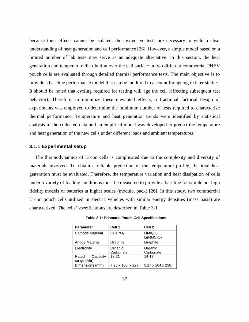
37
because their effects cannot be isolated; thus extensive tests are necessary to yield a clear
understanding of heat generation and cell performance [26]. However, a simple model based on a
limited number of lab tests may serve as an adequate alternative. In this section, the heat
generation and temperature distribution over the cell surface in two different commercial PHEV
pouch cells are evaluated through detailed thermal performance tests. The main objective is to
provide a baseline performance model that can be modified to account for ageing in later studies.
It should be noted that cycling required for testing will age the cell (affecting subsequent test
behavior). Therefore, to minimize these unwanted effects, a fractional factorial design of
experiments was employed to determine the minimum number of tests required to characterize
thermal performance. Temperature and heat generation trends were identified by statistical
analysis of the collected data and an empirical model was developed to predict the temperature
and heat generation of the new cells under different loads and ambient temperatures.
3.1.1 Experimental setup
The thermodynamics of Li-ion cells is complicated due to the complexity and diversity of
materials involved. To obtain a reliable prediction of the temperature profile, the total heat
generation must be evaluated. Therefore, the temperature variation and heat dissipation of cells
under a variety of loading conditions must be measured to provide a baseline for simple but high
fidelity models of batteries at higher scales (module, pack) [26]. In this study, two commercial
Li-ion pouch cells utilized in electric vehicles with similar energy densities (mass basis) are
characterized.Thecells’specificationsaredescribedinTable 3-1.
Table 3-1: Prismatic Pouch Cell Specifications
Parameter Cell 1 Cell 2
Cathode Material LiFePO4 LiMn2O4 Li(NMC)O2
Anode Material Graphite Graphite
Electrolyte Organic Carbonate
Organic Carbonate
Rated Capacity range (Ahr)
18-21 14-17
Dimensions (mm) 7.25 x 160. x 227 5.27 x 164 x 250.
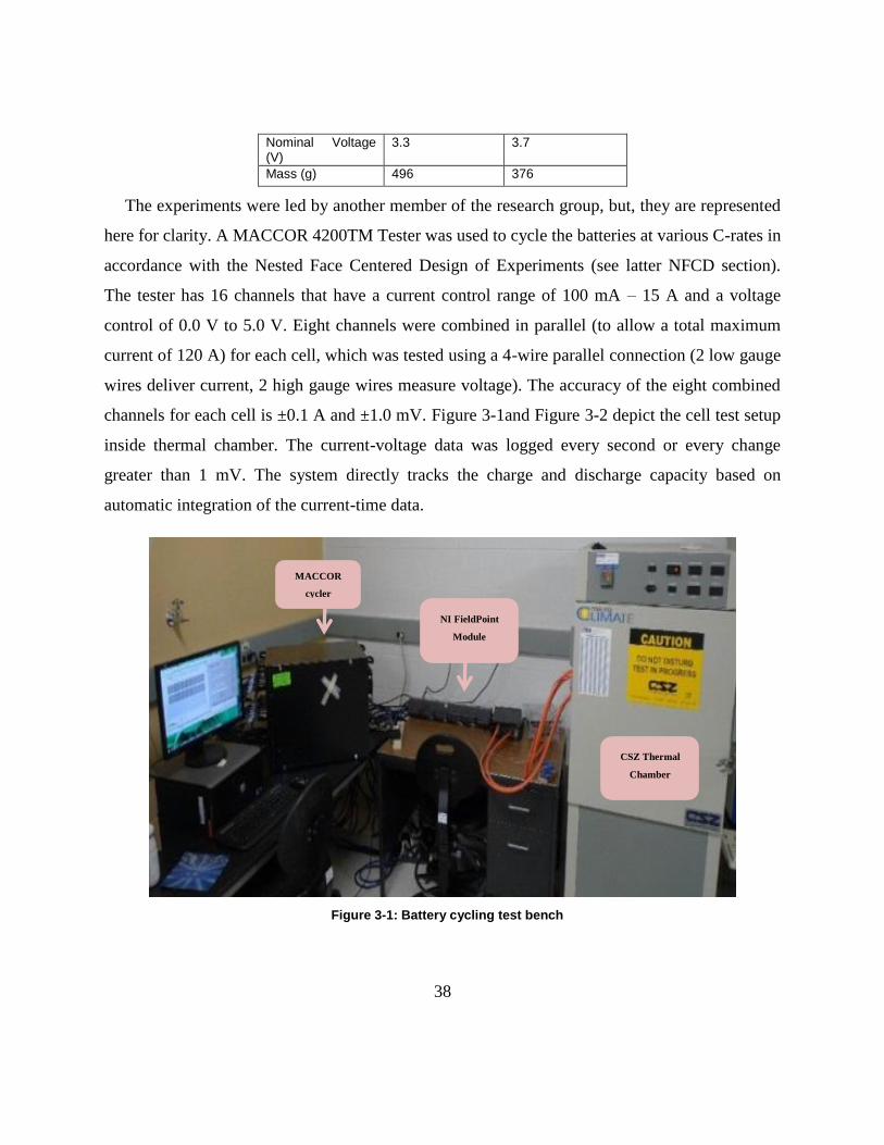
38
Nominal Voltage (V)
3.3 3.7
Mass (g) 496 376
The experiments were led by another member of the research group, but, they are represented
here for clarity. A MACCOR 4200TM Tester was used to cycle the batteries at various C-rates in
accordance with the Nested Face Centered Design of Experiments (see latter NFCD section).
The tester has 16 channels that have a current control range of 100 mA – 15 A and a voltage
control of 0.0 V to 5.0 V. Eight channels were combined in parallel (to allow a total maximum
current of 120 A) for each cell, which was tested using a 4-wire parallel connection (2 low gauge
wires deliver current, 2 high gauge wires measure voltage). The accuracy of the eight combined
channels for each cell is ±0.1 A and ±1.0 mV. Figure 3-1and Figure 3-2 depict the cell test setup
inside thermal chamber. The current-voltage data was logged every second or every change
greater than 1 mV. The system directly tracks the charge and discharge capacity based on
automatic integration of the current-time data.
Figure 3-1: Battery cycling test bench
CSZ Thermal
Chamber
MACCOR
cycler
NI FieldPoint
Module
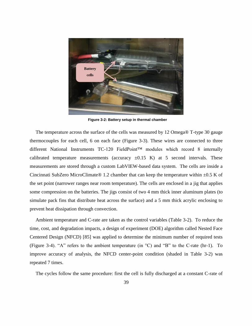
39
Figure 3-2: Battery setup in thermal chamber
The temperature across the surface of the cells was measured by 12 Omega® T-type 30 gauge
thermocouples for each cell, 6 on each face (Figure 3-3). These wires are connected to three
different National Instruments TC-120 FieldPoint™ modules which record 8 internally
calibrated temperature measurements (accuracy ±0.15 K) at 5 second intervals. These
measurements are stored through a custom LabVIEW-based data system. The cells are inside a
Cincinnati SubZero MicroClimate® 1.2 chamber that can keep the temperature within ±0.5 K of
the set point (narrower ranges near room temperature). The cells are enclosed in a jig that applies
some compression on the batteries. The jigs consist of two 4 mm thick inner aluminum plates (to
simulate pack fins that distribute heat across the surface) and a 5 mm thick acrylic enclosing to
prevent heat dissipation through convection.
Ambient temperature and C-rate are taken as the control variables (Table 3-2). To reduce the
time, cost, and degradation impacts, a design of experiment (DOE) algorithm called Nested Face
Centered Design (NFCD) [85] was applied to determine the minimum number of required tests
(Figure 3-4). “A” refers to the ambient temperature (in °C) and “B” to theC-rate (hr-1). To
improve accuracy of analysis, the NFCD center-point condition (shaded in Table 3-2) was
repeated 7 times.
The cycles follow the same procedure: first the cell is fully discharged at a constant C-rate of
Battery
cells

40
1C and then at the constant cut-off voltage until the C-rate is reduced to C/20. The cells are then
rested until thermal and chemical equilibrium is reached; equilibrium here is defined practically
as a change in voltage smaller than 5 mV over a period of half an hour or a total rest time
exceeding 2 hours. The cell is then fully charged from 0% to 100% SOC via constant current (C-
rate specified by the NFCD) and then constant voltage at the upper voltage limit until C/20. The
cell is rested again until equilibrium is achieved and then discharged at constant current
(specified by the NFCD) and then at the cut-off voltage until a C-rate of C/20. The cell is
allowed to rest once more and then the procedure is repeated for a different charge and discharge
current.
Figure 3-3: Thermocouple placement on cell surface
In some instances at low temperatures, the current limits exceeded the manufacturer’s
operating specifications for one of the batteries. In these cases the cell was cycled at the
minimum current, then at the halfway point between the min current and the limit, and finally at
the limit. The heat generation was then estimated based on these results and the model
developed.
Table 3-2: Resulting test points from NFCD
Factor Min (-) Mid points Max (+)
A (ºC) -10 1.25 12.5 23.75 35.0
B (hr-1
) Dis 0.50 1.50 2.50 3.50 4.50
Chg 0.30 0.80 1.30 1.80 2.30

41
Figure 3-4: A two factor NFCD used for thermal studies
3.1.2 Analysis of results
The analysis is split into three sub-sections. The temperature distribution is examined first to
evaluate the accuracy of using a mean temperature in representing the data. Heat generation is
analyzed in the second section. The cell efficiencies are examined in the third section, Greater
emphasis is placed in the second section due to its greater relevance to automotive applications.
Temperature Distribution
In order to quantify the heat generated, it is often assumed that the heat generation inside the
cell is homogeneous, i.e. the heat is conducted very quickly so that only very small temperature
variations exist. However, commercial batteries contain different heterogeneous (diverse in
character) materials with different heat transport and generation properties, some of which are
known to be anisotropic (direction dependent, such as LiFePO4). Further, the asymmetric
arrangement of the different material layers may cause asymmetric heat distributions in at least
one dimension.
Statistical analysis of surface temperature variations across thermocouples placements, makes
it possible to determine whether the temperature (and, subsequently, heat generation) is
uniformly or normally distributed. If this is the case, then a mean heat generation rate for the cell
as a whole can be assumed rather than determining localized rates (as would be required for
complex heterogeneous systems).
As previously mentioned, 32 cycles were conducted for each cell with 12 thermocouple

42
readings every 5 seconds throughout the cycle. In order to decrease the computational time and
complexity of the analysis, the statistical analysis presented only considers instantaneous
measurementsat0%,50%,and100%SOCforallcycles.These‘snapshots’mustbe considered
with the error of the thermocouples in mind (±0.15 K accounting for systematic errors) as well as
naturally occurring temperature distributions within the chamber (which correspond to the
temperature measurements at the initial SOC at the beginning of each charge/discharge step).
Statistics for the 12 thermocouple placements were calculated at each snapshot. The
difference between mean and median, the coefficient of skewness and the standard deviation are
of particular interest. The former two are indicators of the presence and relevance of a skewed
distribution which could point out short-comings in using the mean temperature to represent the
entire cell. The latter quantifies the magnitude of spread among the recorded temperature values.
The coefficient of skewness was also calculated [86] according to:
𝛾1 =√𝑛(𝑛 − 1)
𝑛 − 2
1𝑛∑ (𝑇𝑖 − 𝜇)
3𝑛𝑖=1
(√1𝑛∑ (𝑇𝑖 − 𝜇)
2𝑛𝑖=1 )
3 (3-1)
Where n is 12 (thermocouple temperatures)andμisthemeantemperaturebetweenthese12
readings. The coefficient of skewness should be 0 for any centralized distribution (e.g. normal,
Laplace, student t-distribution, uniform) [87]. Any deviation from that value will be the result of
a skew, with the sign indicating the direction of the skew. Based on the statistical analysis, it can
be stated that the mean is generally an accurate and centered representation of the temperature
distribution and that the heat generation is either uniform, normally distributed with a small
variance, or that at least the surface materials are conductive enough to keep the surface
temperature of the battery even (such that it is unlikely that there would be large temperature
variations within a single cell). Therefore the subsequent heat generation analysis will utilize the
mean temperature in order to quantify the heat generated by the battery. Details of the statistical
analysis can be found in Appendix A.
43
Heat generation
The main objective of the thermal experiments is to calculate the heat generated during each
cycling period. The total heat generated according to the theory can be expressed by:
��𝑔𝑒𝑛 = 𝐼(𝑉𝑂𝐶 − 𝑉) + 𝑇𝐼𝑑𝑉𝑂𝐶𝑑𝑇
(3-2)
Where, VOC represents the open circuit voltage; I, is the current applied and V the cell
terminal voltage. The first and second terms on the right hand side (RHS) of Equation (3-2)
represent the irreversible and reversible heat generation, respectively. However, the term dVOC
dT is
difficult to measure and the difference between open circuit potential and applied voltage is not
easily determinable. Hence, using the recorded cell surface temperatures, it would be more
practical to apply energy balance to calculate the generated heat:
��𝑔𝑒𝑛 = 𝑚𝐶𝑝𝑑𝑇𝑐𝑒𝑙𝑙𝑑𝑡
+ ℎ𝐴(𝑇𝑐𝑒𝑙𝑙 − 𝑇∞) (3-3)
Where, ‘m’ is the cellmass(kg). Cp, is the specific heat(kJ
kgK) ; and ‘h’ is the overall heat
transfer coefficient(W
m2K). The first term on RHS of Equation (3-3) refers to the portion of heat
generated that is translated into the cell temperature change and the second term is the heat
rejected to ambient (simplified) where heat loss through radiation is assumed to be small and is
incorporated within the overall heat transfer coefficient. It is necessary to first estimate the
overall heat transfer coefficient of the cells. Examining the cell temperature curves during the
rest periods (i.e. after charging or discharging, when the current is zero) it can be noted that the
cell temperature approaches the ambient temperature at the end of rest. The temperature
(cooling) curves during these periods can be used for estimating the heat transfer coefficient.
During the rest period no heat is generated as the current is zero, hence Equation (3-3) is
simplified to:
∫mCpdTcelldt
= ∫hA(Tcell − T∞) (3-4)
Integrating over the rest period time results in:
44
∫dTcell
Tcell − T∞=
Tend of rest
T0
hA
mCptrest
(3-5)
Considering the initial conditions: t= 0 and T = T0, and allowing hA
mCp= ∝ the cell
temperature at any point of the rest period (trest) can be expressed as:
Tcell = T∞ + (T0 − T∞) exp (−∝ trest) (3-6)
Cell temperature at the end of each rest period was compared against the measured values in
the tests andusingleastsquarelinearregressioninMATLAB,αwasestimatedas8.5 × 10−4 (s-
1) for Cell 1 and 11 × 10−4 (s-1) for Cell 2. As an example, modeled cooling curves are plotted
against the measurements for the 23.75 ℃ ambient temperatures for Cell 1 in Figure 3-5. Given
that the mass ratio (mBatt1
mBatt2= 1.32) and the respective α coefficient ratio (
∝Batt2
∝Batt1= 1.29) are
almost equivalent we can determine that both cells have similar overall heat transfer coefficients
and therefore dissipate heat at similar rates. This is not surprising since the cells have similar
geometry and contain materials with similar properties (e.g. both have copper and aluminum
current collectors and thin plastic enclosing).Itmustalsobenotedthatαcoefficientsaretime-
averaged over the duration of the rest period and may vary along with fluctuations of air
circulation patterns in the thermal chamber.

45
Figure 3-5: LiFePO4 Cell temperature changes during rest period at 23.75 °C- measured against fitted values
Having estimated suitable values for the heat loss coefficient, the charge and discharge
periods where heat is generated can now be analyzed. Figure 3-6 through Figure 3-9 show the
cell temperature profile at high-mid-low chamber temperatures and lowest and highest C-rates
for charge and discharge tested. At lower temperatures the cells experience higher temperature
rise due to increased cell resistance and therefore decreased efficiency can be expected.
Increasing the C-rate also results in higher temperature increase over the test cycle as dictated by
Equation (3-2) (as well as a decrease in the charge and discharge capacity). The next step in the
analysis is to calculate the heat generation rate and also the accumulated generated heat which is
simply calculated based on Equation (3-2).
0 1000 2000 3000 4000 5000 6000 7000 800022
24
26
28
30
32
34
36
Time (s)
Tem
pe
ratu
re (
°C)
1.8 C-rate charge
1.3 C-rate charge
1.5 C-rate discharge
2.5 C-rate discharge
3.5 C-rate discharge
0.8 C-rate Charge
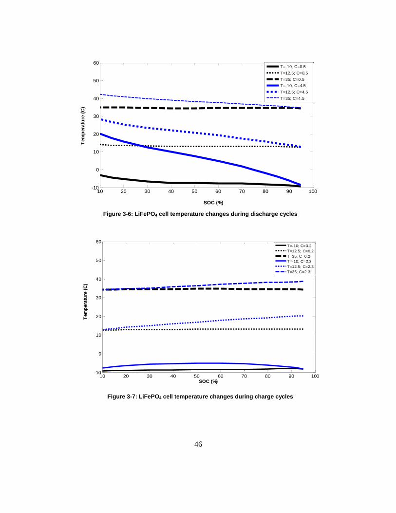
46
Figure 3-6: LiFePO4 cell temperature changes during discharge cycles
Figure 3-7: LiFePO4 cell temperature changes during charge cycles
10 20 30 40 50 60 70 80 90 100-10
0
10
20
30
40
50
60
SOC (%)
Tem
pera
ture
(C
)
T=-10; C=0.5
T=12.5; C=0.5
T=35; C=0.5
T=-10; C=4.5
T=12.5; C=4.5
T=35; C=4.5
10 20 30 40 50 60 70 80 90 100-10
0
10
20
30
40
50
60
SOC (%)
Tem
pera
ture
(C
)
T=-10; C=0.2
T=12.5; C=0.2
T=35; C=0.2
T=-10; C=2.3
T=12.5; C=2.3
T=35; C=2.3

47
Figure 3-8: LiMn2O4 cell temperature changes during discharge cycles
Figure 3-9: LiMn2O4 cell temperature changes during charge cycles
At each SOC, the accumulated heat is calculated with reference to either 100% SOC (for
discharge) or 0% SOC (for charge) as:
10 20 30 40 50 60 70 80 90 100-20
-10
0
10
20
30
40
50
60
SOC (%)
Tem
pera
ture
(C
)
T=35; C=4.5
T=12.5; C=3.56
T=-10; C=1.22
T=12.5; C=0.5
T=-10; C=0.5
T=35; C=0.5
10 20 30 40 50 60 70 80 90 100-20
-10
0
10
20
30
40
50
60
SOC (%)
Tem
pera
ture
(C
)
T=12.5; C=.3
T=35; C=0.3
T=-10; C=0.3
T=12.5; C=1.4
T=-10; C=0.51
T=35; C=2.3

48
𝑄𝑎𝑐𝑐 = ∫ 𝑄𝑔𝑒𝑛𝑑𝑒𝑠𝑖𝑟𝑒𝑑 𝑠𝑜𝑐
𝑠𝑜𝑐 0% 𝑜𝑟 100%
𝑑𝑡 (3-7)
Figure 3-10 through Figure 3-13 show the accumulated heat of the cell at different ambient
temperatures and C-rates. Both cells generated more heat in lower temperatures which results in
a less efficient operation. Also, it is observed that the heat generation is linear between 95% -
20% SOC, the operating range of PHEVs. However the end regions exhibit increased heat
generation rates (0-10% for discharge and 95-100% for charge). This jump in the heat generation
is related to increased resistance, possibly from mass transport or side reactions occurring in the
cells at very high and very low SOCs. This region is increased at lower temperatures and higher
SOCs, suggesting mass transport limitations are the cause of the increased resistance.
Figure 3-10: LiFePO4 cell cumulative heat during discharge cycles
10 20 30 40 50 60 70 80 90 100-5000
0
5000
10000
15000
20000
SOC (%)
Cu
mu
lati
ve
he
at
(J)
T=12.5; C=1.5
T=23.75; C=1.5
T=1.25; C=1.5
T=12.5; C=2.5
T=23.75; C=2.5
T=35; C=2.5
T=-10; C=2.5
T=1.25; C=2.5
T=12.5; C=3.5
T=23.75; C=3.5
T=1.25; C=3.5
T=35; C=4.5
T=12.5; C=4.5
T=-10; C=4.5
T=12.5; C=0.5
T=-10; C=0.5
T=35; C=0.5
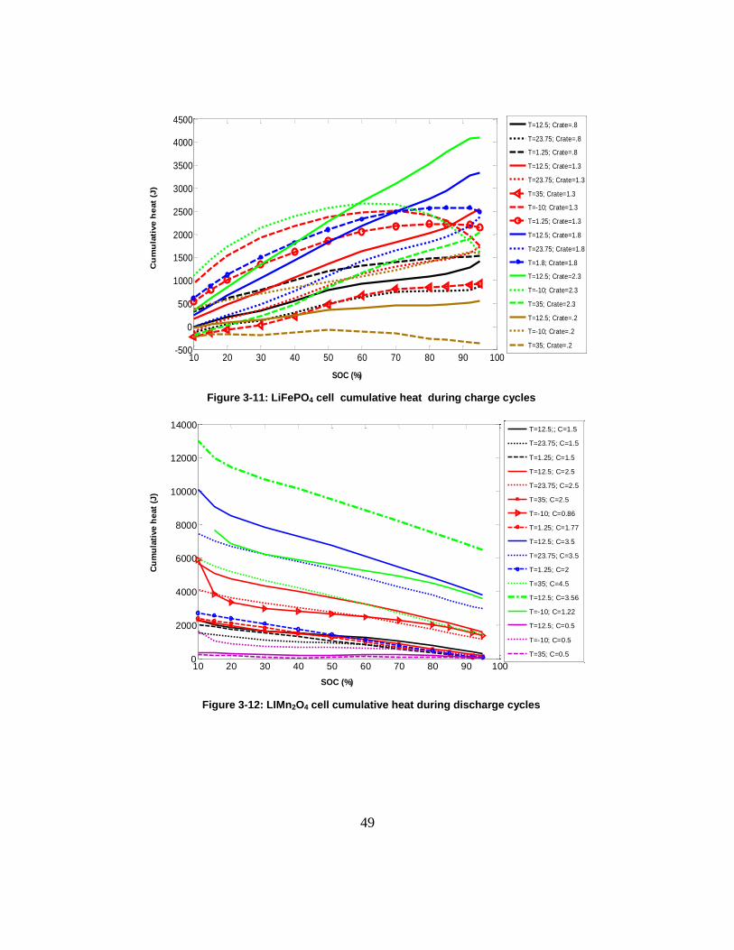
49
Figure 3-11: LiFePO4 cell cumulative heat during charge cycles
Figure 3-12: LIMn2O4 cell cumulative heat during discharge cycles
10 20 30 40 50 60 70 80 90 100-500
0
500
1000
1500
2000
2500
3000
3500
4000
4500
SOC (%)
Cu
mu
lati
ve
he
at
(J)
T=12.5; Crate=.8
T=23.75; Crate=.8
T=1.25; Crate=.8
T=12.5; Crate=1.3
T=23.75; Crate=1.3
T=35; Crate=1.3
T=-10; Crate=1.3
T=1.25; Crate=1.3
T=12.5; Crate=1.8
T=23.75; Crate=1.8
T=1.8; Crate=1.8
T=12.5; Crate=2.3
T=-10; Crate=2.3
T=35; Crate=2.3
T=12.5; Crate=.2
T=-10; Crate=.2
T=35; Crate=.2
10 20 30 40 50 60 70 80 90 1000
2000
4000
6000
8000
10000
12000
14000
SOC (%)
Cu
mu
lati
ve
he
at
(J)
T=12.5;; C=1.5
T=23.75; C=1.5
T=1.25; C=1.5
T=12.5; C=2.5
T=23.75; C=2.5
T=35; C=2.5
T=-10; C=0.86
T=1.25; C=1.77
T=12.5; C=3.5
T=23.75; C=3.5
T=1.25; C=2
T=35; C=4.5
T=12.5; C=3.56
T=-10; C=1.22
T=12.5; C=0.5
T=-10; C=0.5
T=35; C=0.5

50
Figure 3-13: LiMn2O4 cell cumulative heat during charge cycles
Battery efficiencies
A significant factor in reducing the operating cost and increasing the service life of all hybrid
and electric vehicles is to maximize utilization of the energy stored in the battery. In this regard,
ensuring its efficiency remains at a specified performance level is important, not only for
calculationsoftruecostof‘fuel’(electricalenergy)andrangeprediction,butalsoforendoflife
determination and repurposing applications. There are several efficiencies defined for batteries
[88] which will be employed in this section. It is believed that some, if not all, efficiencies
decrease through the lifetime of the battery (with ageing). It is therefore possible that these
efficiencies could be measured on-board as a diagnostic tool for determining the SOH of the
battery. In order to establish a baseline for the batteries, the effects of temperature and C-rate
must be established. In this section, such a baseline for three efficiencies will be established and
discussed.
Electrical Efficiency: sometimes referred to as energy efficiency, it is defined as the ratio of
electrical energy that can be removed from the battery to the electrical energy supplied:
10 20 30 40 50 60 70 80 90 100-1000
-500
0
500
1000
1500
2000
SOC (%)
Cu
mu
lati
ve
he
at
(J)
T=12.5; C=0.3
T=35; C=0.3
T=10; C=0.3
T=12.5; C=0.8
T=23.75; C=08
T=1.25; C=0.75
T=12.5; C=1.3
T=23.75; C=1.3
T=35; C=1.3
T=1.25; C=0.78
T=-10; C=0.38
T=12.5; C=1.4
T=23.75; C=1.8
T=1.25; C=0.82
T=-10; C=0.51
T=35; C=2.3

51
𝜂𝑒𝑙𝑒𝑐𝑡𝑟𝑖𝑐𝑎𝑙 =∫(𝑉𝐼)𝑑𝑖𝑠𝑑𝑡
∫(𝑉𝐼)𝑐ℎ𝑔𝑑𝑡 (3-8)
This efficiency is not observed carefully by vehicle manufacturers but it has important
implications to the vehicle driver. Essentially, it tells the driver how much usable electrical
energy is available based on the previous charge, allowing for an accurate calculation of energy
(fuel) costs. This efficiency was determined over the entire range of SOC, including the constant
voltage portions of the charge and discharge. In practice, the actual electrical efficiency observed
will vary according the usable SOC window within each vehicle application as well as the drive
cycle intensity.
Electrical efficiency of the two cells is reported in Table 3-3 and Table 3-4. In moderate and
high temperatures both cells show to have high electrical efficiency. At low temperatures, both
cells experience decreased electrical efficiency though the impact on the LiFePO4 cell is
significantly greater. In vehicular applications, this effectively translates into a reduced range in
cold weather (as well as higher electricity cost per mile). Increasing the C-rate also decreases the
electrical efficiency suggesting more intense drive cycles will also provide reduced range,
though the impact may not as significant as observed with temperature.
Table 3-3 Electrical efficiency of the LiFePO4 cell
Chamber Temperature (°C)
Discharge C-rate (Charge C-rate is ½ of the discharge)
0.5 1.5 2.5 3.5 4.5
-10.00 78.61
73.40
68.79
1.25 81.36 78.21 75.88
12.50 93.46 88.50 85.36 82.84 80.87
23.75 91.85 89.72 87.67
35.00 97.33 93.23 89.67

52
Table 3-4 Electrical efficiency of the LiMn2O4 cell
Chamber Temperature (°C)
Discharge C-rate (Charge C-rate is ½ of the discharge)
0.5 1.5 2.5 3.5 4.5
-10.00 89.60 87.80* 85.89*
1.25 89.91 88.91* 88.16*
12.50 96.67 93.63 91.14 89.31 89.13*
23.75 94.97 93.44 91.68
35.00 97.91 95.00 92.17 * The cell was not cycled at the labeled C-rates because these lie beyond manufacturer’s
allowable cycling specifications for that temperature. Instead, it was cycled at the limiting
C-rate (where the column states 3.5 or 4.5), or half-way between the limit and the 0.5 C-
rate (where the column states 2.5).
Coulombic efficiency: defined as the ratio of the discharged capacity to the Ah needed to in
order to bring the battery to the discharge initial state (SOC), expressed as follows:
𝜂𝑐𝑜𝑢𝑙𝑜𝑚𝑏𝑖𝑐 =∫ 𝐼𝑑𝑖𝑠𝑑𝑡
∫ 𝐼𝑐ℎ𝑔𝑑𝑡 (3-9)
Where, Idis and Ichg refer to the discharge and charge current respectively and the SOC is the
same at the beginning of discharge and at the end of charge.
Several factors affect the coulombic efficiency, such as charge and discharge current and
charging method (constant voltage/power/current). The occurrence of secondary chemical
reactions (especially at high SOCs) also significantly reduces the coulombic efficiency; i.e.
charging at high SOCs is less efficient [89]. It is therefore possible to examine coulombic
efficiency in order to estimate the extent of electrochemical side reactions occurring in the cells.
Coulombic and electrical efficiency are related to each other through the voltage efficiency
which is defined as the ratio of the average voltage during discharge to the average voltage
during charge[88]:
𝜂𝑒𝑙𝑒𝑐𝑡𝑟𝑖𝑐𝑎𝑙 = 𝜂𝑐𝑜𝑢𝑙𝑜𝑚𝑏𝑖𝑐 × 𝜂𝑣𝑜𝑙𝑡𝑎𝑔𝑒 (3-10)
The coulombic efficiency of the cells over the range of 0% to 100% SOC was found to be
99% or higher for all instances except for cell 1 at 0.5C and -10°C where it was 97.58%. The
cells show a high coulombic efficiency which is reasonable as both cells were fresh at the time of
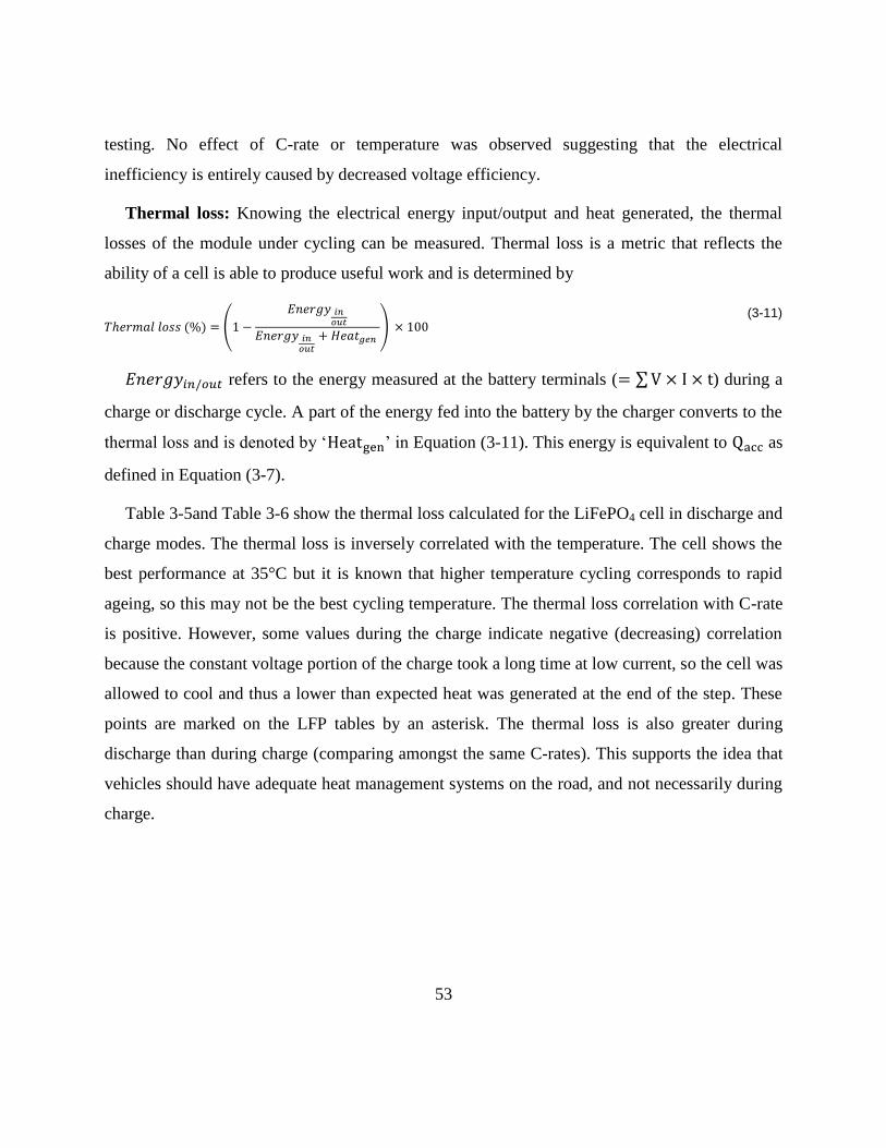
53
testing. No effect of C-rate or temperature was observed suggesting that the electrical
inefficiency is entirely caused by decreased voltage efficiency.
Thermal loss: Knowing the electrical energy input/output and heat generated, the thermal
losses of the module under cycling can be measured. Thermal loss is a metric that reflects the
ability of a cell is able to produce useful work and is determined by
𝑇ℎ𝑒𝑟𝑚𝑎𝑙 𝑙𝑜𝑠𝑠 (%) = (1 −
𝐸𝑛𝑒𝑟𝑔𝑦 𝑖𝑛𝑜𝑢𝑡
𝐸𝑛𝑒𝑟𝑔𝑦 𝑖𝑛𝑜𝑢𝑡
+ 𝐻𝑒𝑎𝑡𝑔𝑒𝑛 ) × 100
(3-11)
𝐸𝑛𝑒𝑟𝑔𝑦𝑖𝑛/𝑜𝑢𝑡 refers to the energy measured at the battery terminals (= ∑V × I × t) during a
charge or discharge cycle. A part of the energy fed into the battery by the charger converts to the
thermallossandisdenotedby‘Heatgen’inEquation (3-11). This energy is equivalent to Qacc as
defined in Equation (3-7).
Table 3-5and Table 3-6 show the thermal loss calculated for the LiFePO4 cell in discharge and
charge modes. The thermal loss is inversely correlated with the temperature. The cell shows the
best performance at 35°C but it is known that higher temperature cycling corresponds to rapid
ageing, so this may not be the best cycling temperature. The thermal loss correlation with C-rate
is positive. However, some values during the charge indicate negative (decreasing) correlation
because the constant voltage portion of the charge took a long time at low current, so the cell was
allowed to cool and thus a lower than expected heat was generated at the end of the step. These
points are marked on the LFP tables by an asterisk. The thermal loss is also greater during
discharge than during charge (comparing amongst the same C-rates). This supports the idea that
vehicles should have adequate heat management systems on the road, and not necessarily during
charge.
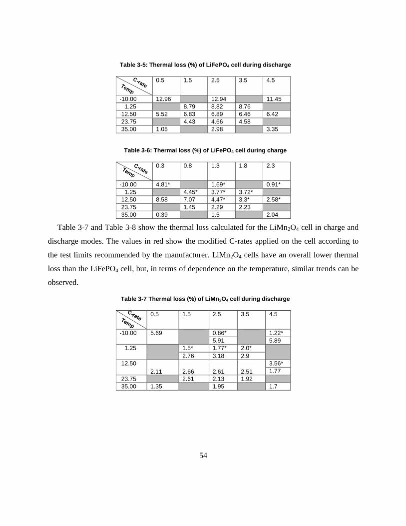
54
Table 3-5: Thermal loss (%) of LiFePO4 cell during discharge
0.5 1.5 2.5 3.5 4.5
-10.00 12.96 12.94 11.45
1.25 8.79 8.82 8.76
12.50 5.52 6.83 6.89 6.46 6.42
23.75 4.43 4.66 4.58
35.00 1.05 2.98 3.35
Table 3-6: Thermal loss (%) of LiFePO4 cell during charge
0.3 0.8 1.3 1.8 2.3
-10.00 4.81* 1.69* 0.91*
1.25 4.45* 3.77* 3.72*
12.50 8.58 expla
7.07 4.47* 3.3* 2.58*
23.75 1.45 2.29 2.23
35.00 0.39 1.5 2.04
Table 3-7 and Table 3-8 show the thermal loss calculated for the LiMn2O4 cell in charge and
discharge modes. The values in red show the modified C-rates applied on the cell according to
the test limits recommended by the manufacturer. LiMn2O4 cells have an overall lower thermal
loss than the LiFePO4 cell, but, in terms of dependence on the temperature, similar trends can be
observed.
Table 3-7 Thermal loss (%) of LiMn2O4 cell during discharge
0.5 1.5 2.5 3.5 4.5
-10.00 5.69 0.86* 1.22*
5.91 5.89
1.25 1.5* 1.77* 2.0*
2.76 3.18 2.9
12.50
2.11 2.66 2.61 2.51
3.56*
1.77
23.75 2.61 2.13 1.92
35.00 1.35 1.95 1.7

55
Table 3-8 Thermal loss (%) of LiMn2O4 cell during charge
0.3 0.8 1.3 1.8 2.3
-10.00
1.13
0.38* 0.51*
0.62 3.85
1.25 0.75* 0.78* 0.82*
0.64 1.83 1.47
12.50 1.43*
0.01 0.46 0.38 0.31
23.75 0.47 0.86 0.18
35.00 0.02 0.36 0.89
Model development
Efficient and safe operation of the battery relies on the efficiency of the vehicle battery
thermal management system (BTMS). The BTMS designer must be able to predict the amount of
heat generation and temperature fluctuation of the battery during a driving or charging cycle. For
this purpose, a thermal model is required to enable prediction of battery temperature changes
according to the battery thermodynamic and chemical status. Based on the observed trends in the
cell surface temperature and the heat generation profiles, it is possible to develop a model to
predict the temperature changes and generated heat in the cell as a function of SOC, cell
temperature, ambient temperature and C-rate. A multiple linear regression analysis was
performed on the data of heat generation for charge and discharge separately. Results of
regressions on the cell #1 (LiFePO4) are presented here. A quadratic fit presented in Equation
(3-12) including the interaction terms between the SOC, C-rate, cell temperature and the ambient
temperature, was applied to the data of heat generation rate.
��𝑔𝑒𝑛 = 𝑏1 + 𝑏2𝐶𝑟𝑎𝑡𝑒 + 𝑏3𝑇𝑐𝑒𝑙𝑙 + 𝑏4𝑆𝑂𝐶 + 𝑏5𝐶𝑟𝑎𝑡𝑒2 + 𝑏6𝑆𝑂𝐶
2 + 𝑏7𝑇𝑐𝑒𝑙𝑙2 + 𝑏8𝐶𝑟𝑎𝑡𝑒 × 𝑆𝑂𝐶 + 𝑏9𝐶𝑟𝑎𝑡𝑒 × 𝑇𝑐𝑒𝑙𝑙
+ 𝑏10𝑆𝑂𝐶 × 𝑇𝑐𝑒𝑙𝑙 + 𝑇𝑎𝑚𝑏
(3-12)
The temperature change will be calculated as:
𝑑𝑇
𝑑𝑡= [��𝑔𝑒𝑛 − ℎ𝐴(𝑇𝑐𝑒𝑙𝑙 − 𝑇𝑎𝑚𝑏)]/𝑚𝐶𝑝 (3-13)
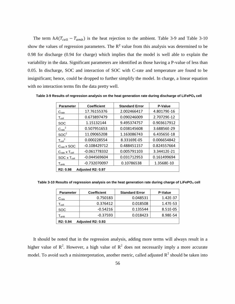
56
The term ℎ𝐴(𝑇𝑐𝑒𝑙𝑙 − 𝑇𝑎𝑚𝑏) is the heat rejection to the ambient. Table 3-9 and Table 3-10
show the values of regression parameters. The R2 value from this analysis was determined to be
0.98 for discharge (0.94 for charge) which implies that the model is well able to explain the
variability in the data. Significant parameters are identified as those having a P-value of less than
0.05. In discharge, SOC and interaction of SOC with C-rate and temperature are found to be
insignificant; hence, could be dropped to further simplify the model. In charge, a linear equation
with no interaction terms fits the data pretty well.
Table 3-9 Results of regression analysis on the heat generation rate during discharge of LiFePO4 cell
Parameter Coefficient Standard Error P-Value
Crate 17.76155376 2.002466417 4.80179E-16
Tcell 0.673897479 0.090246009 2.70729E-12
SOC 1.15132144 9.495374757 0.903617912
Crate2 0.507951653 0.038145608 3.68856E-29
SOC2 11.09065208 1.163086743 6.43565E-18
Tcell2 0.000228554 8.33169E-05 0.006654842
Crate x SOC -0.108429712 0.488451157 0.824557664
Crate x Tcell -0.061778332 0.005791103 3.34412E-21
SOC x Tcell -0.044569604 0.031712953 0.161499694
Tamb -0.732070097 0.10786538 1.3568E-10
R2: 0.98 Adjusted R2: 0.97
Table 3-10 Results of regression analysis on the heat generation rate during charge of LiFePO4 cell
Parameter Coefficient Standard Error P-Value
Crate 0.750183 0.048531 1.42E-37
Tcell 0.376412 0.018508 1.47E-53
SOC -0.54216 0.135544 8.51E-05
Tamb -0.37593 0.018423 8.98E-54
R2: 0.94 Adjusted R2: 0.93
It should be noted that in the regression analysis, adding more terms will always result in a
higher value of R2. However, a high value of R
2 does not necessarily imply a more accurate
model. To avoid such a misinterpretation, another metric, called adjusted R2 should be taken into

57
account. If adjusted R square is significantly lower than R square, this normally means that some
explanatory variable(s) are missing. Also, if adding a new term results in a decreased adjusted
R2, it implies that that term is not significant [90]. Two other diagnostic tools were also used in
this regression analysis: residual plots and normal probability plot. In general, the scatter plot of
the residuals will be disordered if the regression is good. A trend means that the residuals are not
independent (see Figure 3-14). An increasing trend suggests that the error variance increases
with the independent variable; while a distribution with a decreasing trend indicates that the error
variance decreases with the independent variable. Such trends indicate that the assumption of
constant variance (which is assumed in a regression analysis) is not true and the regression is not
reliable [88]. Finally, in a reliable regression model, the normal probability plot should be close
to a line of 45ᵒ slope.
Figure 3-14 Residuals showing a trend (variable variance) [88]
To illustrate the model performance, a comparison is made between the experimental and the
simulated temperature profile of cell #1 at 2.5 C-rate and 23.75ᵒC ambient and shown in

58
Figure 3-15. Also, in Figure 3-16, simulated temperature profile of the cell #1 during charging at
12.5ᵒC and 1.75 C-rate is compared against the measurements. The average error in both cases is
less than 3%.
Figure 3-15 Temperature profile of cell #1 (LiFePO4) during discharge at 2.5 C-rate and 23.75 ᵒC ambient
Figure 3-16 Temperature profile of cell #1 (LiFePO4) during discharge at 1.75 C-rate and 12.5 ᵒC ambient

59
For drive cycle simulations, Equation (3-12) and (3-13) were implemented in
Matlab/Simulink as the battery thermal sub model and integrated to the whole battery model.
Figure 3-17 and Figure 3-18 show the model validation against experiment with US06 drive
cycle at 35ᵒC and 12.5ᵒC. maximum error of 6% and root meat square error (RMSE) of 3% was
observed.
Figure 3-17 Temperature profile of cell #1 (LiFePO4) under US06 profile and 12.5 ᵒC ambient
r
Figure 3-18 Temperature profile of cell #1 (LiFePO4) under US06 profile and 35 ᵒC ambient
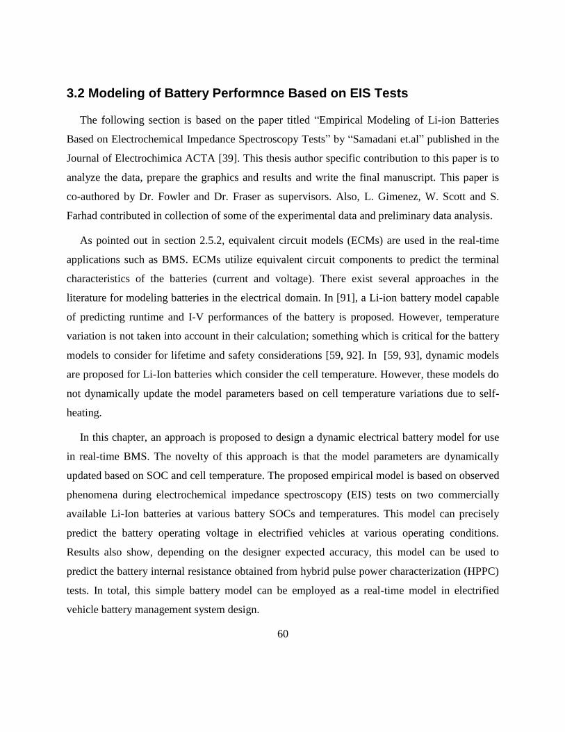
60
3.2 Modeling of Battery Performnce Based on EIS Tests
The following section is based on the paper titled “Empirical Modeling of Li-ion Batteries
Based on Electrochemical Impedance Spectroscopy Tests” by“Samadani et.al”published in the
Journal of Electrochimica ACTA [39]. This thesis author specific contribution to this paper is to
analyze the data, prepare the graphics and results and write the final manuscript. This paper is
co-authored by Dr. Fowler and Dr. Fraser as supervisors. Also, L. Gimenez, W. Scott and S.
Farhad contributed in collection of some of the experimental data and preliminary data analysis.
As pointed out in section 2.5.2, equivalent circuit models (ECMs) are used in the real-time
applications such as BMS. ECMs utilize equivalent circuit components to predict the terminal
characteristics of the batteries (current and voltage). There exist several approaches in the
literature for modeling batteries in the electrical domain. In [91], a Li-ion battery model capable
of predicting runtime and I-V performances of the battery is proposed. However, temperature
variation is not taken into account in their calculation; something which is critical for the battery
models to consider for lifetime and safety considerations [59, 92]. In [59, 93], dynamic models
are proposed for Li-Ion batteries which consider the cell temperature. However, these models do
not dynamically update the model parameters based on cell temperature variations due to self-
heating.
In this chapter, an approach is proposed to design a dynamic electrical battery model for use
in real-time BMS. The novelty of this approach is that the model parameters are dynamically
updated based on SOC and cell temperature. The proposed empirical model is based on observed
phenomena during electrochemical impedance spectroscopy (EIS) tests on two commercially
available Li-Ion batteries at various battery SOCs and temperatures. This model can precisely
predict the battery operating voltage in electrified vehicles at various operating conditions.
Results also show, depending on the designer expected accuracy, this model can be used to
predict the battery internal resistance obtained from hybrid pulse power characterization (HPPC)
tests. In total, this simple battery model can be employed as a real-time model in electrified
vehicle battery management system design.

61
3.2.1 Experiment Setup and Tests Procedure
To be clear for the reader, the experiments are explained in this section. Two commercial Li-
ion pouch cells already described in Table 3-1 were characterized by HPPC and EIS tests over a
range of temperatures and SOCs.
A MACCOR 4200TM
battery cycler was employed for this test and to discharge the cells to the
desired SOC. This cycler has 16 channels with a current control range of 0.1 – 15 A and a
voltage control of 0.0 – 5.0 V for each channel. Eight channels were combined in parallel to
achieve the maximum current of 120 A using a 4-wire parallel connection, where two low gauge
wires deliver current and two high gauge wires measure voltage. The accuracy of the eight
combined channels for each battery was ±0.1 A and ±1.0 mV. The current-voltage data was
logged every second or every change in 1 mV. The HPPC tests were preceded by a full charging
at 1C constant current, followed by constant voltage charging until the current decreased to C/20.
The batteries were then rested until equilibrium was reached. Equilibrium was defined as a
change in voltage smaller than 5 mV over a period of half an hour or a total rest time longer than
2 hours. Afterwards, the batteries were discharged to each test SOC at a rate of 1C, and the
HPPC current profile including a 10 s 5C discharge pulse, a 40 s rest and a 10 s 3.75C
regenerative (charge) pulse was applied and the battery voltage response was measured. The
equipment located at the right in is SubZero MicroClimate® 1.2 temperature control chamber
that maintains the battery temperature within ±0.5 K of the set point. The battery was enclosed in
a vice that simulates a battery pack enclosure (two 4 mm thick inner aluminum plates, which
simulate pack fins that distribute heat across the battery surface, inserted between two 5 mm
thick acrylic plates, which simulate battery casing).
Figure 3-19 illustrates the experimental setup for the EIS test. This test was performed using a
METROHM AutoLAB PGSTAT 302 galvanostat/potentiostat with a current range of ±2 A and a
voltage range of ±10 V. The measurement range for the frequency response analysis is 10 µHz to
1 MHz. The current and voltage accuracy ranges were set to ±10 µA and ±1.0 mV respectively.
To achieve the desired SOC, the battery is fully discharged at a 1C constant current to reach the

62
cut-off voltage and then at the constant cut-off voltage until the current rate is reduced to C/20.
The batteries are then rested until equilibrium is reached; then, the battery is charged to the
desired SOC by coulomb counting at 1.25C current.
Figure 3-19: Experimental setup for the EIS test.
The EIS tests were obtained by scanning 51 points logarithmically spaced between 5 kHz and
5 mHz using a two electrode configuration with the reference and counter electrodes being the
same. The two, rather than three, electrode configuration was chosen due to the difficulty of
placing the third electrode within a sealed commercial pouch cell. The frequency range was
chosen based on analysis of the pertinent parts of the Nyquist plots, and extended to 100 µHz for
some scans at lower temperatures to confirm the presence of the Warburg tail. For the
galvanostatic scans, the baseline current is set to 0 A and the pulse amplitude set to 300 mA. The
batteries were then reconnected to the MACCOR cycler and discharged to the next desired SOC.
Both EIS and HPPC tests were performed at the states of charge of 10%, 30%, 60%, and 90% for
temperatures of 12.5°C, 23.75°C and 35°C. It should be noted that even though the battery might
be exposed to very low or high ambient temperatures in vehicle operation (e.g. aggressive
driving), the BTMS regulates the battery temperature to the optimum range (25-40°C [94]) very
quickly to prevent adverse effects on the cell performance (charge acceptance, power and energy
capability), cycle life, and safety [95]. Therefore this study does not consider extreme
temperatures. The third phase of experiments was measuring the cell response voltage to the
current profile of standard drive cycles (US06, UDDS, and HWFET). For this purpose, a model
EIS
machine

63
of an extended range electric vehicle (EREV), initially developed by UWAFT [96] in Autonomie
software, was used to determine the battery current profile under each of the targeted drive
cycles. The main components of the powertrain of this vehicle are listed in Table 3-11. The
battery pack consists of three parallel strings each including 105 batteries in series (315 batteries
in total). Each drive cycle was applied on the vehicle model and the resulting battery pack
current profile was scaled to a cell level. Afterwards, the cell was cycled under the obtained
current profile for a full discharge by the MACCOR cycler and the voltage response was
recorded.
Table 3-11 Powertrain components specifications of the EREV modified Chevrolet Malibu used in the Autonomie model [45, 96]
Component Option
Engine GM LE9 Engine (E85)
2.4 L E85 engine provided by GM
Generator TM4 Motive (105 kW)
ESS (Battery) Battery Pack (19.7 kWh @ 346 V)
Motor TM4 Motive (206 kW)
Final drive Borg Warner eGearDrive
Chassis 2013 Malibu
Power convertor New Eagle DCDC Converter
Electrical accessory The average power draw from accessories was assumed to be 1500 W
3.2.2 Establishment of the Equivalent Circuit
The observed trends in the Nyquist plots are presented in Figure 3-20 through Figure 3-25.
The number of RC pairs required to describe a cell response is determined from impedance
analysis. For instant, charge transfer reaction is usually modeled by a single RC pair [97]. The
circuit structure is also dependent on cell age and operating conditions. For example, at very low
temperatures additional elements may be required to account for increased resistance as a result
of frozen electrolyte or slow solid diffusion.[98].
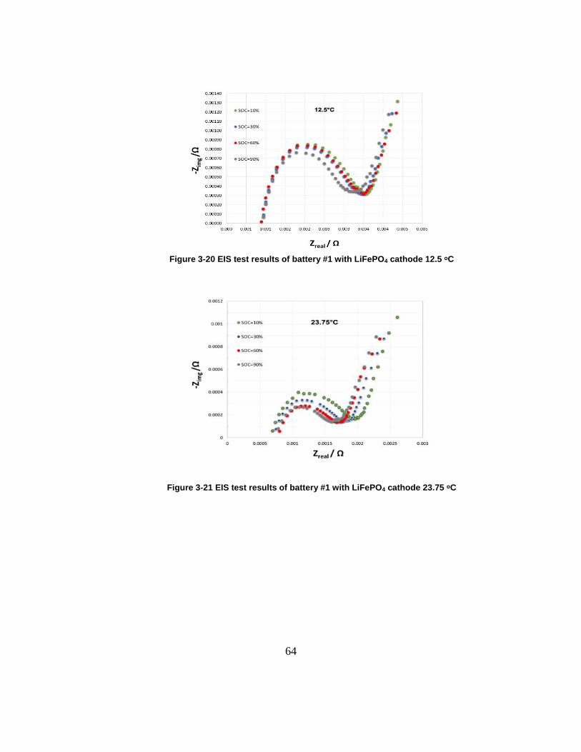
64
Figure 3-20 EIS test results of battery #1 with LiFePO4 cathode 12.5 ᵒC
Figure 3-21 EIS test results of battery #1 with LiFePO4 cathode 23.75 ᵒC

65
Figure 3-22 EIS test results of battery #1 with LiFePO4 cathode 35 ᵒC
Figure 3-23 EIS test results of battery #1 with LiMn2O4
& Li(NMC)O2cathode cathode 12.5 ᵒC

66
Figure 3-24 EIS test results of battery #1 with LiMn2O4
& Li(NMC)O2cathode cathode 23.75 ᵒC
Figure 3-25 EIS test results of battery #1 with LiMn2O4
& Li(NMC)O2cathode cathode 35 ᵒC
Careful investigation of these plots reveals that at most two semicircles with center-points off
the x-axis and a straight line exist in the impedance spectrums. Figure 3-26 shows, two examples
where the response curve includes two semicircles.
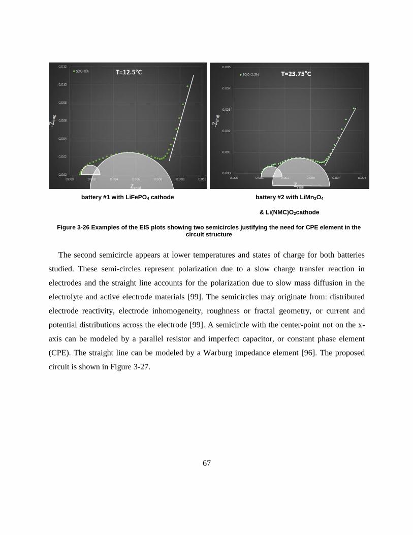
67
battery #1 with LiFePO4 cathode battery #2 with LiMn2O4
& Li(NMC)O2cathode
Figure 3-26 Examples of the EIS plots showing two semicircles justifying the need for CPE element in the circuit structure
The second semicircle appears at lower temperatures and states of charge for both batteries
studied. These semi-circles represent polarization due to a slow charge transfer reaction in
electrodes and the straight line accounts for the polarization due to slow mass diffusion in the
electrolyte and active electrode materials [99]. The semicircles may originate from: distributed
electrode reactivity, electrode inhomogeneity, roughness or fractal geometry, or current and
potential distributions across the electrode [99]. A semicircle with the center-point not on the x-
axis can be modeled by a parallel resistor and imperfect capacitor, or constant phase element
(CPE). The straight line can be modeled by a Warburg impedance element [96]. The proposed
circuit is shown in Figure 3-27.

68
VOC
R1
C1
R2 R3
VBattery
I
W
CPE
Figure 3-27. Proposed equivalent circuit in frequency domain
Because the CPE is a non-intuitive electrical circuit component and cannot be easily
transformed from the frequency to time domain, the CPE was approximated by a perfect
capacitor. Also, it has been shown that the Warburg impedance can be simplified to multiple
parallel RC pairs (as a limiting case, a single RC pair) [100]. In this study, the Warburg element
is replaced by two RC pairs as shown in Figure 3-28. In this fashion, the circuit is simplified to
the one shown in Figure 3-28. The model parameters were determined by an EIS equivalent
circuit solver (Z-man), which uses a genetic mutation algorithm to change model parameters
until the model estimate best approximates measured values. Each circuit component is a
function of SOC and temperature. For each circuit component, this function was determined
through a curve fitting process including all EIS tests points (at various temperatures and SOCs).
VOC
R1
C1
R2
C2
C3 C4
R3
R4 R5VBattery
I
V1 V2 V3
V4 V5
Figure 3-28. Simplification of the proposed circuit for time domain solution.
3.2.3 Parameters Fitting
The equivalent circuit parameter values were determined using Z-man software. Z-man uses

69
the Levenberg-Marquardt algorithm (LMA), or damped least squares method, to minimize the
error between the parameter assigned and empirical values. The parameters of an ECM are
generally a function of temperature and SOC. In case of high degrees of freedom in the model,
due to highly fluctuating trends in the parameters, the designer should try different fittings by
changing initial values using his interpretation and judgment to choose a proper fitting. Also,
imposing restrictions on the parameters would help reduce the degrees of freedom and obtain a
smooth trend for each parameter.
After parameters were determined, they were exported to Microsoft Excel for cross-
comparison. Select data series were then re-evaluated using Z-man software in the event that a
parameter was an outlier. Like most numerical minimization methods, the LMA is an iterative
process and requires an initial guess[101]. When possible, the value of the initial guess was
determined from the previous fitted parameter value. For the initial guess for the first parameter
of a series (e.g. guess SOC0), the Z-man software’s search heuristicmethodwas used. This
heuristic is an evolutionary approach of the particle swarm optimization algorithm. After all
parameters have been fit, they were exposed to cross analysis. When a parameter fit exceeded an
order of magnitude of a previous value, all parameters for that temperature and state of charge
were re-evaluated using the heuristic evolutionary approach until complying with the parameter
series. In the event that the parameter series did not have aligning fits, the entire series was re-
evaluated. As an example, Figure 3-29 and Figure 3-30 show fitted values of R1 (Ohmic
resistance) for both batteries at three temperatures.
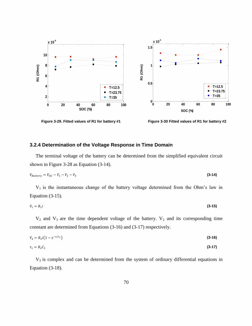
70
Figure 3-29. Fitted values of R1 for battery #1 Figure 3-30 Fitted values of R1 for battery #2
3.2.4 Determination of the Voltage Response in Time Domain
The terminal voltage of the battery can be determined from the simplified equivalent circuit
shown in Figure 3-28 as Equation (3-14).
𝑉𝐵𝑎𝑡𝑡𝑒𝑟𝑦 = 𝑉𝑂𝐶 − 𝑉1 − 𝑉2 − 𝑉3 (3-14)
V1 is the instantaneous change of the battery voltage determined from the Ohm’s law in
Equation (3-15).
𝑉1 = 𝑅1𝑖 (3-15)
V2 and V3 are the time dependent voltage of the battery. V2 and its corresponding time
constant are determined from Equations (3-16) and (3-17) respectively.
𝑉2 = 𝑅2𝑖(1 − 𝑒−𝑡/𝜏1) (3-16)
𝜏1 = 𝑅2𝐶1 (3-17)
V3 is complex and can be determined from the system of ordinary differential equations in
Equation (3-18).
0 20 40 60 80 100
2
4
6
8
10
x 10-4
SOC (%)
R1
(O
hm
)
T=12.5
T=23.75
T=35
0 20 40 60 80 1000
0.5
1
1.5
x 10-3
SOC (%)
R1
(O
hm
)
T=12.5
T=23.75
T=35

71
{
𝜏2
𝑑𝑉3𝑑𝑡
= −𝑉3 + 𝑉4 + 𝑉5 + 𝑅3𝑖
𝜏3𝑑𝑉4𝑑𝑡
= (𝑅4𝑅3) 𝑉3 − (
𝑅4𝑅3+ 1)𝑉4 − (
𝑅4𝑅3)𝑉5
𝜏4𝑑𝑉5𝑑𝑡
= (𝑅5𝑅3)𝑉3 − (
𝑅5𝑅3) 𝑉4 − (
𝑅5𝑅3+ 1)𝑉5
(3-18)
𝜏2, 𝜏3, and 𝜏4 are defined as follows:
𝜏2 = 𝑅3𝐶2 (3-19)
𝜏3 = 𝑅4𝐶3 (3-20)
𝜏4 = 𝑅5𝐶4 (3-21)
The solution of Equation (3-18) employs transformation into the Laplace domain:.
{
ℒ[𝑉3] =
1
(𝜏2𝑠 + 1)ℒ[𝑉4] +
1
(𝜏2𝑠 + 1)ℒ[𝑉5] +
(𝑅3𝑖)
(𝜏2𝑆 + 1)
1
𝑠
ℒ[𝑉4] =(𝑅4𝑅3)
(𝜏3𝑠 + (𝑅4𝑅3+ 1))
ℒ[𝑉3] −(𝑅4𝑅3)
(𝜏3𝑠 + (𝑅4𝑅3+ 1))
ℒ[𝑉5]
ℒ[𝑉5] =(𝑅5𝑅3)
(𝜏4𝑠 + (𝑅5𝑅3+ 1))
ℒ[𝑉3] −(𝑅5𝑅3)
(𝜏4𝑠 + (𝑅5𝑅3+ 1))
ℒ[𝑉4]
(3-22)
After simplification of Equation (3-22), V3 is obtained as Equation (3-23). To take Laplace
inverse from the right side of Equation (3-23), this equation should be written as Equation
(3-24).
𝑉3 = (𝑖)ℒ−1
[
(𝑅3𝜏2) 𝑠2 + (
𝑅3 + 𝑅5𝜏2𝜏4
+𝑅3 + 𝑅4𝜏2𝜏3
) 𝑠 + (𝑅3 + 𝑅4 + 𝑅5
𝜏2𝜏3𝜏4)
𝑠 (𝑠3 + (1𝜏2+1 +
𝑅4𝑅3
𝜏3+1 +
𝑅5𝑅3
𝜏4)𝑠2 + (
1𝜏2𝜏3
+1𝜏2𝜏4
+1 +
𝑅4𝑅3+𝑅5𝑅3
𝜏3𝜏4)𝑠 +
1𝜏2𝜏3𝜏4
)
]
(3-23)
𝑉3 = (𝑅3 + 𝑅4 + 𝑅5)𝑖ℒ−1 [
1
𝑠−
𝐴
(𝑠 + 𝑟1)−
𝐵
(𝑠 + 𝑟2)−
𝐶
(𝑠 + 𝑟3)] (3-24)

72
Where, r1, r2 and r3 in Equation (3-24) are the three real roots of Equation (3-25) as it appeared
in the denominator of Equation (3-23). These three real roots are obtained from Equations (3-26)
to (3-28).
𝑠3 + (1
𝜏2+1 +
𝑅4𝑅3
𝜏3+1 +
𝑅5𝑅3
𝜏4)𝑠2 + (
1
𝜏2𝜏3+
1
𝜏2𝜏4+1 +
𝑅4𝑅3+𝑅5𝑅3
𝜏3𝜏4)𝑠 +
1
𝜏2𝜏3𝜏4 (3-25)
𝑟1 =𝑎
3+
(
2
3(𝑎2 − 3𝑏)0.5𝑐𝑜𝑠 (
𝑎𝑟𝑐𝑐𝑜𝑠 (2𝑎3 − 9𝑎𝑏 + 27𝑐2(𝑎2 − 3𝑏)1.5
)
3)
)
(3-26)
𝑟2 =𝑎
3+
(
2
3(𝑎2 − 3𝑏)0.5𝑐𝑜𝑠 (
𝑎𝑟𝑐𝑐𝑜𝑠 (2𝑎3 − 9𝑎𝑏 + 27𝑐2(𝑎2 − 3𝑏)1.5
) + 2𝜋
3)
)
(3-27)
𝑟3 =𝑎
3+
(
2
3(𝑎2 − 3𝑏)0.5𝑐𝑜𝑠 (
𝑎𝑟𝑐𝑐𝑜𝑠 (2𝑎3 − 9𝑎𝑏 + 27𝑐2(𝑎2 − 3𝑏)1.5
) − 2𝜋
3)
)
(3-28)
Where, a, b, and c are obtained from the following equations:
𝑎 =1
𝜏2+ (1 +
𝑅4𝑅3)1
𝜏3+ (1 +
𝑅5𝑅3)1
𝜏4 (3-29)
𝑏 =1
𝜏2𝜏3+
1
𝜏2𝜏4+ (1 +
𝑅4𝑅3+𝑅5𝑅3)1
𝜏3𝜏4 (3-30)
𝑐 =1
𝜏2𝜏3𝜏4 (3-31)
A, B, and C in Equation (3-24) are determined from Equation (3-32) and (3-33).
𝐴 =𝜏3𝜏4𝑅3𝑟1 +
1𝑟1(𝑅3 + 𝑅4 + 𝑅5) − (𝑅3 + 𝑅5)𝜏3 − (𝑅3 + 𝑅4)𝜏4
(𝑅3 + 𝑅4 + 𝑅5)(𝜏2𝜏3𝜏4)(𝑟1 − 𝑟2)(𝑟1 − 𝑟3) (3-32)
𝐵 =𝜏3𝜏4𝑅3𝑟2 +
1𝑟2(𝑅3 + 𝑅4 + 𝑅5) − (𝑅3 + 𝑅5)𝜏3 − (𝑅3 + 𝑅4)𝜏4
(𝑅3 + 𝑅4 + 𝑅5)(𝜏2𝜏3𝜏4)(𝑟2 − 𝑟1)(𝑟2 − 𝑟3) (3-33)

73
𝐶 =𝜏3𝜏4𝑅3𝑟3 +
1𝑟3(𝑅3 + 𝑅4 + 𝑅5) − (𝑅3 + 𝑅5)𝜏3 − (𝑅3 + 𝑅4)𝜏4
(𝑅3 + 𝑅4 + 𝑅5)(𝜏2𝜏3𝜏4)(𝑟3 − 𝑟1)(𝑟3 − 𝑟2)
(3-34)
After determination of r1, r2, r3, A, B, and C and taking Laplace inverse from Equation (3-24) ,
V3 is determined as:
𝑉3 = (𝑅3 + 𝑅4 + 𝑅5)𝑖[1 − 𝐴𝑒−𝑟1𝑡 − 𝐵𝑒−𝑟2𝑡 − 𝐶𝑒−𝑟3𝑡] (3-35)
Substituting Equations (3-15), (3-16) and (3-35) into Equation (3-14), the battery voltage is
determined as Equation (3-36)
𝑉𝐵𝑎𝑡𝑡𝑒𝑟𝑦(𝑡) = 𝑉𝑂𝐶 − 𝑅1𝑖 − 𝑅2𝑖(1 − 𝑒−𝑡/𝜏1) − (𝑅3 + 𝑅4 + 𝑅5)𝑖[1 − 𝐴𝑒
−𝑟1𝑡 − 𝐵𝑒−𝑟2𝑡 − 𝐶𝑒−𝑟3𝑡] (3-36)
In Equation (3-36), the battery current is positive on discharge and negative in change. This
equation is suitable to determine the voltage response when a constant current is drawn from the
battery. However, under a drive cycle operation, the battery current profile shows high
fluctuations due to instantaneous changes in the power demand. Therefore, Equation (3-36)
should be modified to account for the effect of a time varying current profile on the battery
voltage. For this purpose, the current profile is binned into constant current segments. The
voltage response for the first bin is calculated form Equation (3-37) where the battery starts from
equilibrium state.
𝑉𝐵𝑎𝑡𝑡𝑒𝑟𝑦,1(𝑡) = 𝑉𝑂𝐶 − 𝑅1𝑖1 − 𝑅2𝑖1 (1 − 𝑒−𝑡𝜏1)
− (𝑅3 + 𝑅4 + 𝑅5)𝑖1[1 − 𝐴𝑒−𝑟1𝑡 − 𝐵𝑒−𝑟2𝑡 − 𝐶𝑒−𝑟3𝑡] (0 ≤ 𝑡 < 𝑡1)
(3-37)
For other segments, the voltage response is considered to be a function of the current applied
in that segment as well as the current applied in previous segments; therefore, Equation (3-37) is
modified to Equation (3-38), where, the term 𝑉𝐵𝑎𝑡𝑡𝑒𝑟𝑦,𝑗(𝑡) referstothebatteryvoltageattime“t”
in the segment “j” and 𝑉𝐵𝑎𝑡𝑡𝑒𝑟𝑦,𝑗−1(𝑡), refers to the battery voltage at the time “t” due to the
currentapplied in theprevioussegment ‘j-1’.“𝑖𝑗 − 𝑖𝑗−1” is thedifferencebetween theapplied
current in the two adjacent segments.

74
𝑉𝐵𝑎𝑡𝑡𝑒𝑟𝑦,𝑗(𝑡) = 𝑉𝐵𝑎𝑡𝑡𝑒𝑟𝑦,𝑗−1(𝑡) − 𝑅1(𝑖𝑗 − 𝑖𝑗−1) − 𝑅2(𝑖𝑗 − 𝑖𝑗−1) (1 − 𝑒−(𝑡−𝑡𝑗−1)
𝜏1 )
− (𝑅3 + 𝑅4 + 𝑅5)(𝑖𝑗 − 𝑖𝑗−1)[1 − 𝐴𝑒−𝑟1(𝑡−𝑡𝑗−1) − 𝐵𝑒−𝑟2(𝑡−𝑡𝑗−1)
− 𝐶𝑒−𝑟3(𝑡−𝑡𝑗−1)] (𝑡𝑗−1 ≤ 𝑡 < 𝑡𝑗) & (𝑗 ≥ 2)
(3-38)
Where the values of VOC, R1, R2, R3, R4, R5, A, B, C, 1, r1, r2, r3 were updated with the
current state of charge of the battery obtained from Equation (3-39).
Δ(𝑆𝑂𝐶) = −𝑖𝑗Δ𝑡
𝑄𝐵𝑎𝑡𝑡𝑒𝑟𝑦 (3-39)
The model parameters are a function of temperature and SOC. Therefore, a 2-D look up table
was created which updates the parameters according to the instantaneous SOC and temperature.
The temperature is updated by a thermal sub model which predicts the cell temperature changes
according to its losses and convection to the ambient already presented in the section 3.1.
3.2.5 Results and Discussion
Verification of the proposed model is accomplished in two stages. First, the ability of the
model is evaluated for prediction of the battery internal resistances obtained from HPPC tests.
Second, the model is studied under standard drive cycles for output potential difference
predictions in a hypothetical EREV. The focus of this section will be the battery with a LFP
cathode, and the model validation is performed mainly for the LFP battery. It should be noted
that the SOC window considered for the simulations is 10 to 90 % due to two observations: first,
the HPPC test does not provide reliable results at extreme SOCs, and second, the BMS is
designed to limit the battery from being over charged or discharged.
Cell 1 (LFP Cathode)
To verify the accuracy of the proposed empirical model, the model was run under HPPC
current profile (as shown in ) and the resultant battery internal resistances were compared with
those obtained from a Thevenin model [65] as well as HPPC tests. The Hybrid Pulse Power
Characterization (HPPC) test, recommended by the U.S. Department of Energy FreedomCAR

75
battery test manual [102], is used for cell characterization in terms of internal resistance and
power capability at different SOCs and temperatures.
Figure 3-31 : HPPC test- pulse power characterization profile
Several studies have utilized the HPPC method to fit a simple RC circuit or internal resistance
(Rint) model for simplicity and ease of implementation [12, 103, 104]. Another study employs a
simple RC model to predict the mean pack behavior and a Rint model to simulate differences
between the individual cells [105]. EIS provides an alternative approach to defining the circuit
parameters[22, 106]. Unlike the HPPC test, EIS does not assume that battery response is
unaffected by pulse duration or that there is no significant time delay between input and
response. These assumptions have been shown to be false through examination of Nyquist plots
used in EIS studies [22, 107]. In addition, the HPPC test, when compared to EIS, has been shown
to impose more stress on the battery [108]. Lastly, compared to HPPC, EIS test facility is much
more economical; therefore, it would be desirable to verify the possibility of replacing HPPC test
with EIS.
Results of comparison for the battery with LFP cathode at temperatures of 12.5°C, 23.75°C
and 35°C are shown in Figure 3-32. It is observed that the proposed model better matches the
experimental results than the Thevenin model. An average error of 20 % is observed in values

76
predicted by the proposed empirical model. Further investigations also revealed that the
empirical model can predict the charge resistances of both batteries with an average error of
about 13%. Charge and discharge error may be reduced by increasing the number of EIS tests
(e.g. from four SOCs to eight). Additionally, replacing the perfect capacitors C1 and C2 with
CPEs would incorporate the effects of: distributed electrode reactivity, electrode inhomogeneity,
roughness or fractal geometry, and the current and potential distributions across the electrode,
which could further reduce model error.

77
Figure 3-32. Comparison of discharge resistances obtained from HPPC tests and modeling for the battery with LFP cathode at different temperatures.
The model was further evaluated by simulating the cell voltage profile over three standard
drive cycles (US06, UDDS, and HWFET). The cycle current profiles were separately
aggregated and applied to the proposed, Thevenin, and simple resistance (Rint) models. Resulting
battery voltages were compared with the experimental data over a 90% to 10% SOC range. The
voltage obtained from the model and experiment for this battery at operating temperature of
35°C is shown in Figure 3-33. As seen in this figure, there is an excellent agreement between the
model and experiment. At this temperature, the highest error was observed during the US06
drive cycle with an average error of 1.2% and the maximum instantaneous error of 5.3%.

78
HWFET
Figure 3-33. Comparison of the battery voltage obtained from the empirical model and experiment for the battery with LFP cathode at 35°C standard EPA drive cycles.
10 20 30 40 50 60 70 80 90
3
3.1
3.2
3.3
3.4
3.5
3.6
SOC (%)
Ou
tpu
t p
ote
nti
al d
iffe
ren
ce
/ V
US06
Model
Experiment
0.1 0.2 0.3 0.4 0.5 0.6 0.7 0.8 0.9 13.1
3.15
3.2
3.25
3.3
3.35
3.4
3.45
SOC (%)
Ou
tpu
t p
ote
nti
al
dif
fere
nce
/ V
UDDS Model
Experiment
605040302010 70 80 90
10 20 30 40 50 60 70 80 903.1
3.15
3.2
3.25
3.3
3.35
3.4
3.45
3.5
SOC (%)
Ou
tpu
t p
ote
nti
al
dif
fere
nce
/ V
HWFET
Model
Experiment
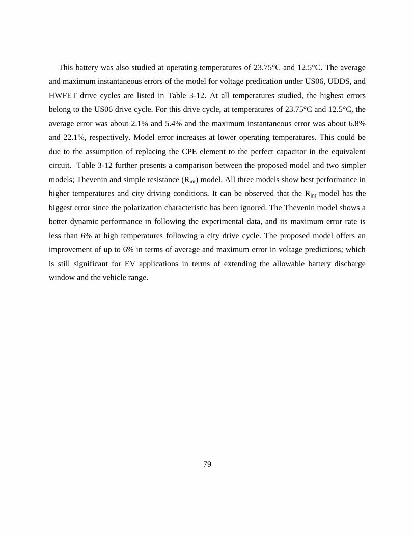
79
This battery was also studied at operating temperatures of 23.75°C and 12.5°C. The average
and maximum instantaneous errors of the model for voltage predication under US06, UDDS, and
HWFET drive cycles are listed in Table 3-12. At all temperatures studied, the highest errors
belong to the US06 drive cycle. For this drive cycle, at temperatures of 23.75°C and 12.5°C, the
average error was about 2.1% and 5.4% and the maximum instantaneous error was about 6.8%
and 22.1%, respectively. Model error increases at lower operating temperatures. This could be
due to the assumption of replacing the CPE element to the perfect capacitor in the equivalent
circuit. Table 3-12 further presents a comparison between the proposed model and two simpler
models; Thevenin and simple resistance (Rint) model. All three models show best performance in
higher temperatures and city driving conditions. It can be observed that the Rint model has the
biggest error since the polarization characteristic has been ignored. The Thevenin model shows a
better dynamic performance in following the experimental data, and its maximum error rate is
less than 6% at high temperatures following a city drive cycle. The proposed model offers an
improvement of up to 6% in terms of average and maximum error in voltage predictions; which
is still significant for EV applications in terms of extending the allowable battery discharge
window and the vehicle range.
80
Table 3-12. Average and maximum errors of the proposed empirical model for voltage prediction of the battery with LFP cathode in various drive cycles over 90% to 10% SOC.
Drive cycle
Average error (%) Maximum error (%)
Proposed
model Thevenin Rint
Proposed
model Thevenin Rint
@ 35 (ᵒC)
US06 1.2 1.4 3.8 5.3 5.9 12.9
UDDS 0.6 0.8 0.8 2.5 3.7 3.9
HWFET 1.1 1.3 1.4 3.6 4.1 7.5
@ 23.75 (ᵒC)
US06 2.1 2.2 3.2 6.8 8.2 12.9
UDDS 1.2 1.5 1.6 4.2 5.3 5.6
HWFET 1.8 1.9 1.9 4.5 4.6 7.7
@ 12.5 (ᵒC)
US06 5.4 5.7 6.1 22.1 22.8 23.8
UDDS 2.3 3.1 3.8 10.4 11.5 13.1
HWFET 4.6 4.7 5.1 13.7 14.3 15.2
Cell 2 (Composite LMO & NMC Cathode)
Figure 3-34 illustrates the results of the discharge resistances obtained from HPPC tests
through modeling and experiment for the battery with composite LMO & NMC cathode. As
before, the results corresponding to the empirical model, as compared to the Thevenin model,
better follow the experimental with the empirical model resistances averaging 12 % error. An
average error of 10 % is observed in the predicted charge resistances for this battery. The
proposed model can be further evaluated if drive cycle test data is made available for the LMO &
NMC battery.

81
Figure 3-34. Comparison of discharge resistances obtained from HPPC tests and modeling for the battery with composite LMO & NMC cathode at different temperatures.
82
3.2.6 Impact of convection coefficient on the temperature profile
One important design criteria of battery operation is that the battery temperature stays smooth
and within a controllable range to maintain optimal performance. In this section, the sensitivity
of the battery temperature rise to the convection coefficient is investigated. For this purpose, the
battery model (DPW) is run under different convection coefficient ranging from 1h (2 W/m2K),
corresponding to the natural convection, to 10h (~20 W/m2K) resembling a mild forced
convection condition. As the plots in Figure 3-35 suggest, a convection coefficient value of 7.5h
(15 W/m2K) would result in a saturated temperature profile with minimum fluctuation over
different drive cycles; which is an affordable value and could be fulfilled by using a fan. Also, in
Figure 3-35 (4) effect of the convection coefficient on the battery maximum temperature rise
under different drive cycles is illustrated. This plot reassures the feasibility of designing a
thermal management unit for the cells with minimal temperature fluctuations.
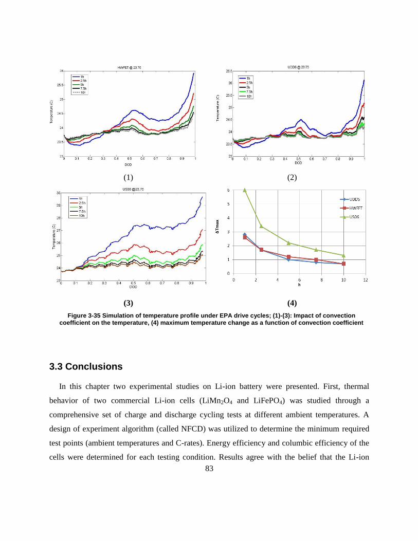
83
(1) (2)
(3) (4)
Figure 3-35 Simulation of temperature profile under EPA drive cycles; (1)-(3): Impact of convection coefficient on the temperature, (4) maximum temperature change as a function of convection coefficient
3.3 Conclusions
In this chapter two experimental studies on Li-ion battery were presented. First, thermal
behavior of two commercial Li-ion cells (LiMn2O4 and LiFePO4) was studied through a
comprehensive set of charge and discharge cycling tests at different ambient temperatures. A
design of experiment algorithm (called NFCD) was utilized to determine the minimum required
test points (ambient temperatures and C-rates). Energy efficiency and columbic efficiency of the
cells were determined for each testing condition. Results agree with the belief that the Li-ion

84
cells have a better performance at higher temperatures. The temperature distribution of the cells
was found to be approximately uniform within the confines of the experimental error. Also, heat
generation of the cells was calculated assuming natural convection mechanism for heat rejection
to the ambient. It is planned to validate the calculated heat generation against the theoretical heat
generation inside the cell. Finally, a statistical model of the temperature and also cumulative
generated heat was developed for each cell (charge and discharge).
In the second section, a simple real-time empirical model for voltage prediction of Li-ion
batteries was developed based on the observed phenomena at various battery states of charge and
temperatures under EIS test. It was shown that this model can precisely predict the battery
voltage during various drive cycles of electrified vehicles. The model was compared with both
the simple resistance and Thevenin models and up to 6% improvement in the battery voltage
prediction was observed. The model was also evaluated in terms of predicting the HPPC test
results. The investigations confirmed the model capability in following the HPPC test trends
within about 20% error. This error can be significantly reduced by using CPEs instead of perfect
capacitors in the equivalent circuit model. In this condition, the effects of distributed electrode
reactivity, electrode inhomogeneity, and distributed current and potential across the electrode
could be considered. This model is desirable to designers as an alternative method for the HPPC
test, as this test imposes stress to the battery and its setup is expensive for high capacity batteries
and battery packs. Although the model developed was based on data of two commercial Li-ion
batteries, this modeling approach is applicable to model Li-ion batteries of different chemistries.

85
Chapter 4
Battery Characterization through Field Tests
Thefollowingsectionismainlybasedonthepapertitled“ModelingandEvaluationofLi-Ion
BatteryPerformanceBasedontheElectricVehicleFieldTests”by“Samadani et.al”published
by the Society of automotive Engineer (SAE). This thesis author specific contribution to this
paper is conducting the experiment, analyzing the data, preparing the graphics and results and the
final manuscript. This paper is co-authored by Dr. Fowler and Dr. Fraser as supervisors. Also, L.
S. Farhad assisted with advice in the data analysis.
Although Li-ion battery offers many advantages such as high specific power and capacity,
their performance and reliability in actual EV application need to be further verified. In this
context, a systematic approach is required to enable assessment of the operational requirements
specific to EV applications. This chapter describes the results of a research conducted for the
Burlington Hydro as a part of its GridSmartCityTM
project [109]. The results are based on the
field testconductedonanelectrifiedFordEscape2009which is apartofBurlingtonHydro’s
fleet and is equipped with three packs of cylindrical Li-ion battery (LiFePO4) including an
overall 20 modules in series. Through monitoring various performance and utilization parameters
of an EV, this study provides practical in-situ data on EV operation and grid electricity
requirements and helps addressing the following key technical issues of EVs and their
connection to the grid:
Charging and charge management;
Applicability as a fleet vehicle;
Vehicle performance modeling; and;
Li-ion battery degradation modeling.
As the ultimate objective of this study, an attempt has been made to bridge the gap between
laboratory studies and real life environment and to study the battery degradation in real-life

86
conditions. There are many factors that affect the Li-ion battery performance and health. Also, in
EV applications, battery health is known to be very much dependent on the driving and charging
habit. Therefore, there is a growing desire to evaluate the path dependence of battery
degradation. This is due to the fact that lab environment is far different from what the battery
experiences under real operation in EVs and relying solely on the results of lab testing may cause
a great mislead in estimating the battery state of health (SOH) and remaining life. However, real-
life testing is expensive and labor intensive and is associated with a very low level of control ;
therefore it has not been the subject of researches very much so far [32]. In the following
sections, the data management system installed on the vehicle, and the powertrain and battery
characterization and modeling are presented.
4.1 Data Management System and Battery Packs
Figure 4-1 shows the converted EV under study. There are three packs of Li-ion battery
installed on the vehicle; including a total of 20 battery modules in series. Figure 4-2 shows a
schematic of the battery packs locations in the vehicle. Each module contains 6serisesx49parallel
IFR18650e cylindrical Valence cells. The data management system consists of a data logger
installed in the vehicle, a cellular network data connection for data collection, and processing
scripts that convert the logged data into monthly usage reports. The data logger unit records data
from the battery, powertrain, and GPS. A list of recorded signals that are necessary for modeling
of vehicle performance and battery degradation is presented in Table 4-1. The data logger is
installed beneath the front passenger seat and connects to the vehicle controller area network bus
(CANBus). The global positioning system (GPS) unit is mounted on the ceiling of the passage
cabin near the central mirror to reduce the possibility of poor satellite acquisition. The data
recording unit (DRU) and modem are located beneath the front passenger seat. The data logger is
powered by the existing 12V battery in the vehicle.Figure 4-3 shows the data recorder unit seat
and Figure 4-4 shows the data logger connection and shut down wire in vehicle. The ‘shut
down’wire isused toautomaticallypower-off the recorder and its peripherals after 4 hours of
inactivity. The cellular antenna that enables wireless data transmission is located on top of the

87
car.
Figure 4-1 Converted Ford Escape (EV-ACX2.5) Figure 4-2. integration of multiple batteries packs [110]
Table 4-1 Data logging signals
Component Recorded Signal significance
Battery
Voltage & current
SOC
Temperature
Verify vehicle energy use and regenerative braking
Verify battery health status as both extreme temperature and SOCs are known to escalate degradation
Electric motor Voltage & current
Speed
Torque
Monitor powertrain energy use
Vehicle Speed & Acceleration Monitor vehicle performance
Figure 4-3: Data recorder unit Figure 4-4: Data logger connection and shut down
wire
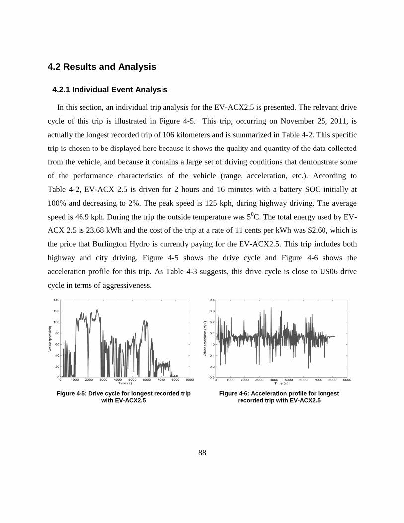
88
4.2 Results and Analysis
4.2.1 Individual Event Analysis
In this section, an individual trip analysis for the EV-ACX2.5 is presented. The relevant drive
cycle of this trip is illustrated in Figure 4-5. This trip, occurring on November 25, 2011, is
actually the longest recorded trip of 106 kilometers and is summarized in Table 4-2. This specific
trip is chosen to be displayed here because it shows the quality and quantity of the data collected
from the vehicle, and because it contains a large set of driving conditions that demonstrate some
of the performance characteristics of the vehicle (range, acceleration, etc.). According to
Table 4-2, EV-ACX 2.5 is driven for 2 hours and 16 minutes with a battery SOC initially at
100% and decreasing to 2%. The peak speed is 125 kph, during highway driving. The average
speed is 46.9 kph. During the trip the outside temperature was 50C. The total energy used by EV-
ACX 2.5 is 23.68 kWh and the cost of the trip at a rate of 11 cents per kWh was $2.60, which is
the price that Burlington Hydro is currently paying for the EV-ACX2.5. This trip includes both
highway and city driving. Figure 4-5 shows the drive cycle and Figure 4-6 shows the
acceleration profile for this trip. As Table 4-3 suggests, this drive cycle is close to US06 drive
cycle in terms of aggressiveness.
Figure 4-5: Drive cycle for longest recorded trip with EV-ACX2.5
Figure 4-6: Acceleration profile for longest recorded trip with EV-ACX2.5

89
Table 4-2 Cycle details, November 25, 2011
Trip Time 2 hour,16 min
Trip Distance 106 km
Starting SOC 100 %
Ending SOC 2 %
Total Energy -23.68 kWh
Cycle Average Speed 46.92 kph
Cycle Peak Speed 125 kph
Average Positive Acceleration 0.59 m/s2
Peak Positive Acceleration 3.43 m/s2
Trip Cost (at $ 0.11/kWh) 2.60 CAD
Cost per km (at $0.11/kWh) 0.024 CAD/km
Outside Temperature +5 0C
Table 4-3: Acceleration comparison between Nov25 drive cycle and standard drive cycles
Cycle Maximum acceleration (m/s2) Average acceleration (m/s2)
UDDS 1.47 0.55
HWFET 1.43 0.19
US06 3.75 0.67
Nov25-EV-ACX2.5 3.43 0.59
Figure 4-7 and Figure 4-8 show the battery voltage and current profiles for the trip. The
minimum battery voltage is 350 V and the maximum battery voltage is 414 V. It can be observed
that there is a decreasing trend in the battery terminal voltage which is a result of continuous
loading on the battery packs during driving. The peak battery discharge current is -195 A and the
peak battery regenerative braking current is 100 A. Thus, the peak battery discharge power is -
68.25 kW and peak regenerative braking charge power is 43.88 kW. Figure 4-9 also shows the
SOC profile of the battery for this trip. There is a drastic reduction in SOC between 1000 sec to
3000 sec because during this time span, the vehicle was highway driven with very high speed of
120 kph. After 3000 sec, a fluctuating trend in the SOC curve is observed which is due to the in-
city driving condition where regenerative braking frequently occurs.

90
Figure 4-7: Battery voltage profile for longest recorded trip with EV-ACX2.5
Figure 4-8: Battery current profile for longest recorded trip with EV-ACX2.5
Figure 4-9: Battery SOC profile for longest recorded trip with EV-ACX2.5
Figure 4-10 depicts the battery maximum and minimum temperature profiles (as measured
over all of the battery modules) as a function of time for this trip. It is very well known that the
heat generation from a battery is due to resistive (I2R) losses and the enthalpy changes due to
electrochemical reactions during discharge or charge. Heat generation rate from a battery module
depends on several parameters like battery temperature, initial and final state of charge, charge
and discharge rate and profile and also on chemistry and construction. The EV-ACX2.5 uses 20
passively cooled battery modules located in three packaged locations on the vehicle. It is evident
that these different locations are causing significant differences in cell temperature over the drive
cycle. These differences may cause differential cell ageing, which can be monitored. Since the
data loggers collect battery voltage, current, and temperature at the module level, degradation
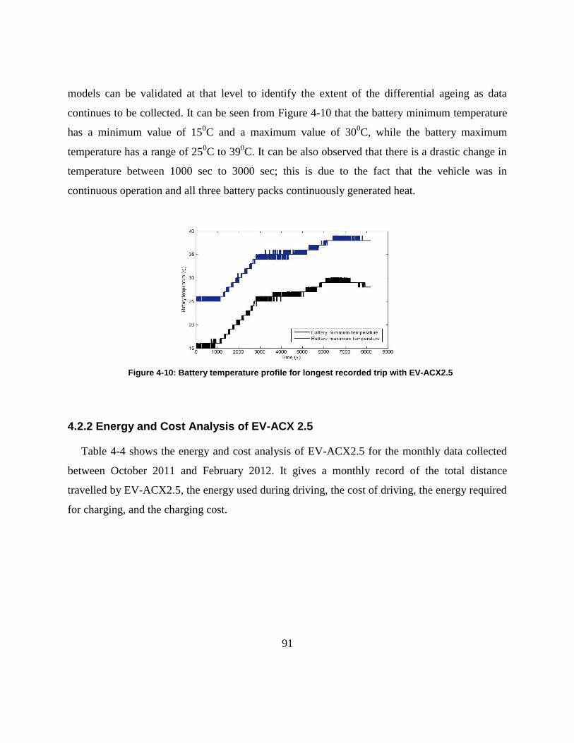
91
models can be validated at that level to identify the extent of the differential ageing as data
continues to be collected. It can be seen from Figure 4-10 that the battery minimum temperature
has a minimum value of 150C and a maximum value of 30
0C, while the battery maximum
temperature has a range of 250C to 39
0C. It can be also observed that there is a drastic change in
temperature between 1000 sec to 3000 sec; this is due to the fact that the vehicle was in
continuous operation and all three battery packs continuously generated heat.
Figure 4-10: Battery temperature profile for longest recorded trip with EV-ACX2.5
4.2.2 Energy and Cost Analysis of EV-ACX 2.5
Table 4-4 shows the energy and cost analysis of EV-ACX2.5 for the monthly data collected
between October 2011 and February 2012. It gives a monthly record of the total distance
travelled by EV-ACX2.5, the energy used during driving, the cost of driving, the energy required
for charging, and the charging cost.
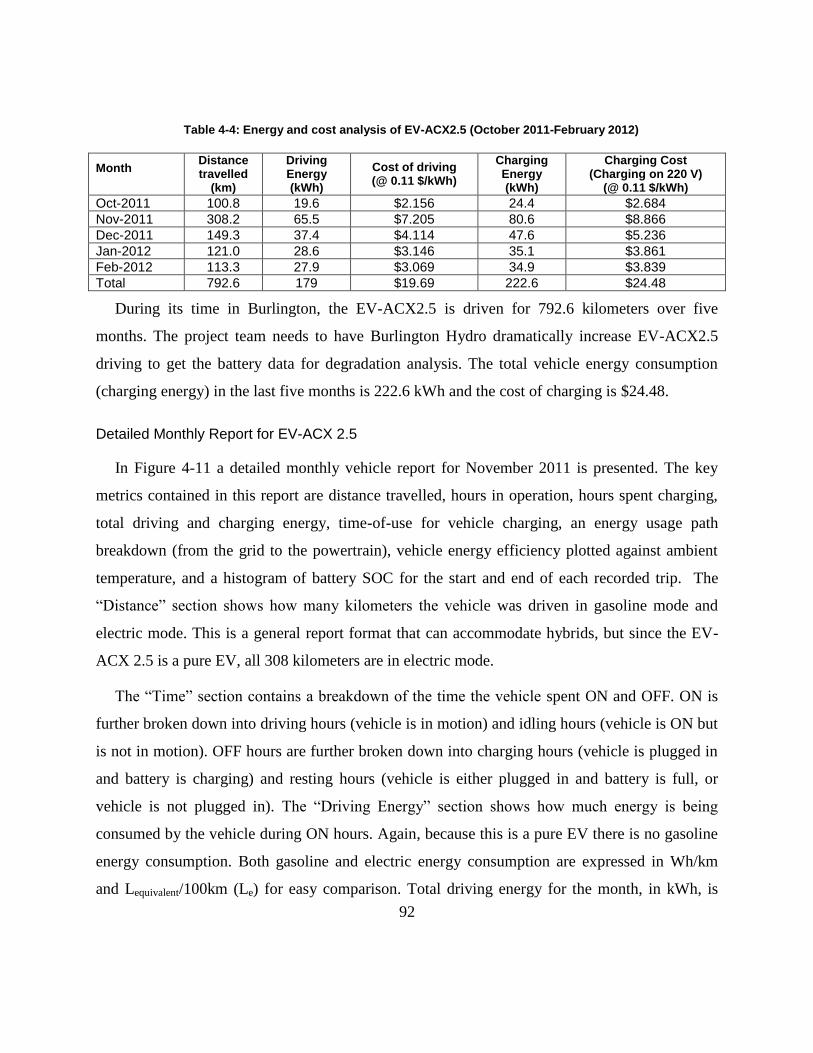
92
Table 4-4: Energy and cost analysis of EV-ACX2.5 (October 2011-February 2012)
Month Distance travelled
(km)
Driving Energy (kWh)
Cost of driving (@ 0.11 $/kWh)
Charging Energy (kWh)
Charging Cost (Charging on 220 V)
(@ 0.11 $/kWh)
Oct-2011 100.8 19.6 $2.156 24.4 $2.684
Nov-2011 308.2 65.5 $7.205 80.6 $8.866
Dec-2011 149.3 37.4 $4.114 47.6 $5.236
Jan-2012 121.0 28.6 $3.146 35.1 $3.861
Feb-2012 113.3 27.9 $3.069 34.9 $3.839
Total 792.6 179 $19.69 222.6 $24.48
During its time in Burlington, the EV-ACX2.5 is driven for 792.6 kilometers over five
months. The project team needs to have Burlington Hydro dramatically increase EV-ACX2.5
driving to get the battery data for degradation analysis. The total vehicle energy consumption
(charging energy) in the last five months is 222.6 kWh and the cost of charging is $24.48.
Detailed Monthly Report for EV-ACX 2.5
In Figure 4-11 a detailed monthly vehicle report for November 2011 is presented. The key
metrics contained in this report are distance travelled, hours in operation, hours spent charging,
total driving and charging energy, time-of-use for vehicle charging, an energy usage path
breakdown (from the grid to the powertrain), vehicle energy efficiency plotted against ambient
temperature, and a histogram of battery SOC for the start and end of each recorded trip. The
“Distance” section shows howmany kilometers the vehicle was driven in gasoline mode and
electric mode. This is a general report format that can accommodate hybrids, but since the EV-
ACX 2.5 is a pure EV, all 308 kilometers are in electric mode.
The“Time”sectioncontainsabreakdownofthetimethevehicle spent ON and OFF. ON is
further broken down into driving hours (vehicle is in motion) and idling hours (vehicle is ON but
is not in motion). OFF hours are further broken down into charging hours (vehicle is plugged in
and battery is charging) and resting hours (vehicle is either plugged in and battery is full, or
vehicle is not plugged in). The “Driving Energy” section shows how much energy is being
consumed by the vehicle during ON hours. Again, because this is a pure EV there is no gasoline
energy consumption. Both gasoline and electric energy consumption are expressed in Wh/km
and Lequivalent/100km (Le) for easy comparison. Total driving energy for the month, in kWh, is

93
also shown.
The“ChargingEnergy” sectionprovidesboth the total charging energyused in the month,
andapercentagebreakdownofhowthosekWhwereobtained.InOntario’stime-of-use (TOU)
pricing system electricity charges per kWh vary depending on the time of day and time of year.
Prices increase as the time moves from off-peak to mid-peak to on-peak, so it is desirable to plan
activities such that the vehicle can be charged off-peak as much as possible. This section also
shows the percentage of charging energy obtained from 110V, 220V, and DC quick charge
stations. It is important to note that the breakdowns in this section are in kWh (energy), not hours
(time). The“EnergyPath”sectionshowswhereenergyisconsumedinthevehicle.Thecharger
energyisthatenergyconsumedbythevehicle’son-board charger in converting grid electricity
from AC to DC energy that is compatible with the vehicle battery. The powertrain energy is the
battery energy consumed by the vehicle to operate. The regenerative energy is the energy
recovered by the regenerative braking system, resulting in reduced powertrain energy. All values
are given per kilometer travelled for that month.
The“Temperature”sectionplotsthevehicle energy consumption in Whkm-1
against ambient
temperature for each recorded trip. This plot is useful for demonstrating the effects of ambient
temperature (and the resulting vehicle climate control energy consumption) on energy efficiency.
The“BatteryCharge”sectionisahistogramofbatterySOC at the start and end of each trip. It
provides an at-a-glance view of the typical battery SOC utilization. The monthly reports for
October 2011, December 2011, January 2012, and February 2012 are provided in Appendix D.
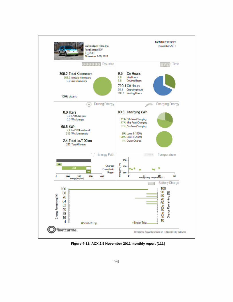
94
Figure 4-11: ACX 2.5 November 2011 monthly report [111]

95
Comparison between EV-ACX 2.5 and HEVs
In order to compare the energy consumption and energy cost of the EV-ACX 2.5 with that of
Burlington Hydro’s other fleet vehicles, drive cycles from two of Burlington Hydro’s Ford
Escape Hybrid (2008 and 2009 model years) fleet vehicles were recorded over four months,
between November 2011 and February 2012. Table 4-5 summarizes the monthly distance travel,
fuel consumption, and the equivalent energy use in kWh for the HEVs. The equivalence ratio of
9.7 kWh per litre is used for gasoline [104] It is seen that HEV #4 has the most utilization of the
two HEVs and yields the richest data set. Therefore further analysis was performed based on the
HEV #4 recorded data to compare the energy usage and cost with EV-ACX2.5. The results are
reported in Table 4-6.
Table 4-5: Distance travelled and energy consumption by fleet vehicles
Month
HEV #3 HEV#4
Distance travelled
(km)
Fuel (L)
Equivalent Energy (kWh)
Distance (km)
Fuel (L)
Equivalent Energy (kWh)
Nov.2011 252.8 21.9 212.43 742.9 51.09 495.57
Dec.2011 - - - 793.48 53.15 515.57
Jan. 2012 150 10.2 98.94 1214 80 776
Feb.2012 104.5682 8.8618 85.95 769.16 50.61 490.917
Table 4-6: Energy and cost comparison between EV-ACX2.5 and HEV#4
Month
HEV#4 ACX 2.5
Distance travelled
(km)
Fuel (L)
Equivalent Energy (Kwh)
(kWh=Lx9.7)
Cost (@11cent
/kWh)
Distance (km)
Energy (kWh) (kWh=Lx9.7)
Cost (@11cent
/kWh)
Nov-2011 742.9 51.09 495.57 $54.51 308.2 65.5 $7.205
Dec-2011 793.48 53.15 515.57 $56.71 149.3 37.4 $4.114
Jan-2012 253.53 80 160.923 $17.70 121 28.6 $3.146
Feb-2012 769.16 50.61 490.917 $54 113.3 27.9 $3.069
Total 3519.54 234.85 2278 $182.92 691.8 159.4 $17.53
Economy 0.0512 ($/km) 0.025 ($/km)
From Table 4-6, it is observed that the EV-ACX2.5 has travelled a much shorter distance over
the last four months as compared to the HEV#4. Over four months, the HEV #4 is driven for
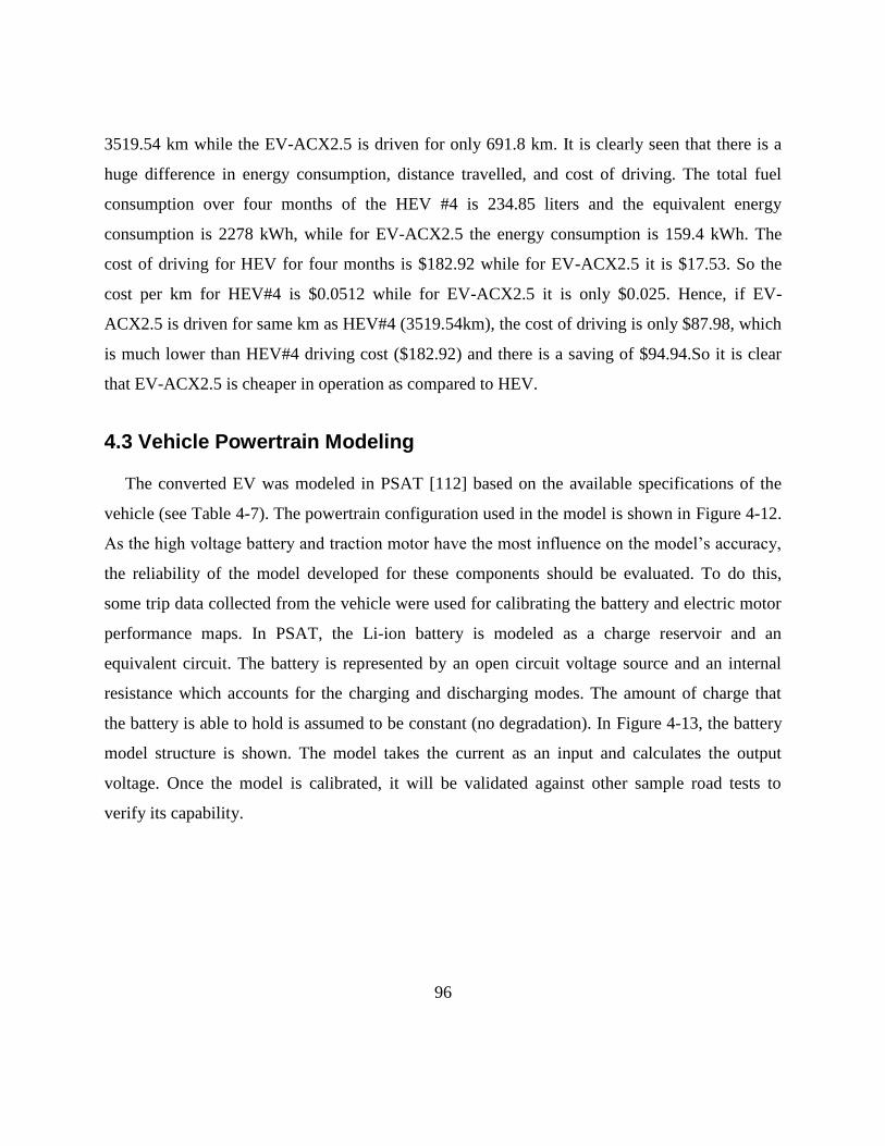
96
3519.54 km while the EV-ACX2.5 is driven for only 691.8 km. It is clearly seen that there is a
huge difference in energy consumption, distance travelled, and cost of driving. The total fuel
consumption over four months of the HEV #4 is 234.85 liters and the equivalent energy
consumption is 2278 kWh, while for EV-ACX2.5 the energy consumption is 159.4 kWh. The
cost of driving for HEV for four months is $182.92 while for EV-ACX2.5 it is $17.53. So the
cost per km for HEV#4 is $0.0512 while for EV-ACX2.5 it is only $0.025. Hence, if EV-
ACX2.5 is driven for same km as HEV#4 (3519.54km), the cost of driving is only $87.98, which
is much lower than HEV#4 driving cost ($182.92) and there is a saving of $94.94.So it is clear
that EV-ACX2.5 is cheaper in operation as compared to HEV.
4.3 Vehicle Powertrain Modeling
The converted EV was modeled in PSAT [112] based on the available specifications of the
vehicle (see Table 4-7). The powertrain configuration used in the model is shown in Figure 4-12.
Asthehighvoltagebatteryandtractionmotorhavethemostinfluenceonthemodel’saccuracy,
the reliability of the model developed for these components should be evaluated. To do this,
some trip data collected from the vehicle were used for calibrating the battery and electric motor
performance maps. In PSAT, the Li-ion battery is modeled as a charge reservoir and an
equivalent circuit. The battery is represented by an open circuit voltage source and an internal
resistance which accounts for the charging and discharging modes. The amount of charge that
the battery is able to hold is assumed to be constant (no degradation). In Figure 4-13, the battery
model structure is shown. The model takes the current as an input and calculates the output
voltage. Once the model is calibrated, it will be validated against other sample road tests to
verify its capability.

97
Table 4-7 Key specifications for the electrified Ford Escape
Specification Value
Mass (Empty) 1814 kg
Motor Peak Power 90 kW
Motor Peak Efficiency 98% at 4000 RPM
Motor Peak Torque 239 Nm
Battery Module Nominal Voltage
19.2 V
Battery Module Energy Density
89 Wh/kg
Battery Module Nominal Capacity
69 Ah
Total Battery Pack Energy Capacity
25 kWh
Typical Range for a full discharge
100 km
Figure 4-12 Drivetrain configuration of the converted EV in PSAT [111]
Figure 4-13 Top level of the battery model in PSAT
In the first step, a drive cycle that is representative of the expected driving conditions is
needed to be developed. To achieve a comprehensive set of data, this cycle should cover a wide
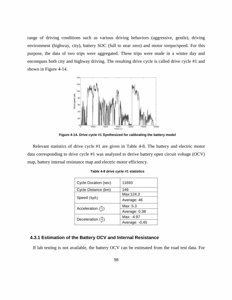
98
range of driving conditions such as various driving behaviors (aggressive, gentle), driving
environment (highway, city), battery SOC (full to near zero) and motor torque/speed. For this
purpose, the data of two trips were aggregated. These trips were made in a winter day and
encompass both city and highway driving. The resulting drive cycle is called drive cycle #1 and
shown in Figure 4-14.
Figure 4-14. Drive cycle #1 Synthesized for calibrating the battery model
Relevant statistics of drive cycle #1 are given in Table 4-8. The battery and electric motor
data corresponding to drive cycle #1 was analyzed to derive battery open circuit voltage (OCV)
map, battery internal resistance map and electric motor efficiency.
Table 4-8 drive cycle #1 statistics
Cycle Duration (sec) 11693
Cycle Distance (km) 149
Speed (kph) Max:124.3
Average: 46
Acceleration (m
s2)
Max: 5.3
Average: 0.38
Deceleration (m
s2)
Max: -4.97
Average: -0.45
4.3.1 Estimation of the Battery OCV and Internal Resistance
If lab testing is not available, the battery OCV can be estimated from the road test data. For

99
this purpose, a scatter plot of battery voltage should be employed. As an example, the battery
voltage profile during a sample driving and corresponding charging profile is illustrated in
Figure 4-15.
Driving; SOC 91-35 %
Charging; SOC 35-99 %
Figure 4-15: Sample battery pack voltage profile
By selecting the minimum load points in the voltage-SOC scatter plot, (where the battery
current < C/20), and fitting a polynomial curve, the approximated value of the battery OCV at
various SOC can be estimated. This method was applied on the drive cycle #1 battery data. To
verify the accuracy of this estimation method, a test was conducted to measure the OCV in a
more realistic way. In this test, through in-city driving, the battery was drained from fully
charged state to almost 0% SOC in intervals of 10% SOC followed by 2 hours rest at each SOC.
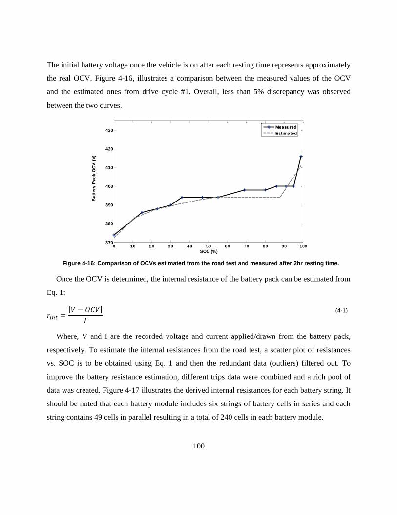
100
The initial battery voltage once the vehicle is on after each resting time represents approximately
the real OCV. Figure 4-16, illustrates a comparison between the measured values of the OCV
and the estimated ones from drive cycle #1. Overall, less than 5% discrepancy was observed
between the two curves.
Figure 4-16: Comparison of OCVs estimated from the road test and measured after 2hr resting time.
Once the OCV is determined, the internal resistance of the battery pack can be estimated from
Eq. 1:
𝑟𝑖𝑛𝑡 =|𝑉 − 𝑂𝐶𝑉|
𝐼
(4-1)
Where, V and I are the recorded voltage and current applied/drawn from the battery pack,
respectively. To estimate the internal resistances from the road test, a scatter plot of resistances
vs. SOC is to be obtained using Eq. 1 and then the redundant data (outliers) filtered out. To
improve the battery resistance estimation, different trips data were combined and a rich pool of
data was created. Figure 4-17 illustrates the derived internal resistances for each battery string. It
should be noted that each battery module includes six strings of battery cells in series and each
string contains 49 cells in parallel resulting in a total of 240 cells in each battery module.
0 10 20 30 40 50 60 70 80 90 100370
380
390
400
410
420
430
SOC (%)
Batt
ery
Pa
ck
OC
V (
V)
Measured
Estimated

101
Figure 4-17: Internal resistance of the battery module derived from data of drive cycle #1
It should be noted that the procedure presented here is solely based on the road test data;
while for measuring the battery resistance in the lab, standard tests are available and all the
parameters are controlled. In a real-life situation, there is almost no control over the
circumstantial factors. Also, the estimation presented here is limited to the specific environment
in which the vehicle is tested. Therefore, to obtain the battery internal resistance from the road
test data under different ambient temperatures, the vehicle road test data in different seasons is
required. Considering the battery aging, namely, the calendar life and cycling life, associated
with this waiting time that may increase the battery internal resistance, one may not be able to
fully differentiate the effect of aging and the ambient temperature.
4.3.2 Model Testing and Validation
The estimated battery OCV and internal resistance are employed to model the battery pack in
PSAT software. To simplify the modeling, a cell level model is up scaled linearly to represent a
pack (unbalancing and cell-to-cell variations are ignored). Figure 4-18 shows the SOC curves
obtained from the model and the road test data (drive cycle #1). As seen in this figure, the model
is able to track the experimental SOC curve with an error of about 3.8%. There are some
discrepancies in the in-city portion of the SOC curve, which is related to the regenerative control
strategies. However, as long as the model is able to track the SOC changes and the battery
0 10 20 30 40 50 60 70 80 90 1000.04
0.06
0.08
0.1
0.12
0.14
0.16
0.18
0.2
0.22
SOC (%)
Batt
ery
Pa
ck
Dis
ch
arg
e R
es
ista
nc
e (
Oh
m)

102
energy consumption, these discrepancies do not significantly affect the modeling accuracy. The
total energy processed in the battery was also examined using the following formula:
𝑇𝑜𝑡𝑎𝑙 𝑒𝑛𝑒𝑟𝑔𝑦 =∑(𝐶𝑢𝑟𝑟𝑒𝑛𝑡 × 𝑉𝑜𝑙𝑡) × 𝑡𝑖𝑚𝑒 (4-2)
Our studies also indicated that the battery model is able to track the total energy drawn from
the battery pack with an error of less than 2.3%.
Figure 4-18: SOC versus time; obtained from the model and drive cycle #1
In addition, based on the scatter plot of torque-speed of the electric motor, the braking control
strategy is modified in order to match the maximum regenerative energy produced by the motor
at different speeds with the test data. Figure 4-19 shows the power flow of the motor calculated
from the model and experiment. An average error 4% was observed in the results.

103
Figure 4-19: Power Flow into the Electric Motor, model and drive cycle #1 (first 8000 sec)
As shown in Figure 4-20, inputs to the motor are the voltage and current coming from the
battery and the outputs are in terms of torque and speed; therefore the overall efficiency of the
motor is calculated as follows:
Figure 4-20. Inputs and Outputs to the Electric Motor
𝜂 =∑(𝑇𝑜𝑟𝑞𝑢𝑒×𝑆𝑝𝑒𝑒𝑑)
∑(𝐶𝑢𝑟𝑟𝑒𝑛𝑡×𝑉𝑜𝑙𝑡𝑎𝑔𝑒)= {
91.7 % (𝑚𝑜𝑑𝑒𝑙) 90 % (𝑒𝑥𝑝𝑟𝑖𝑚𝑒𝑛𝑡)
The model slightly overestimated the efficiency of the electric motor.
Figure 4-21 compares the vehicle acceleration from the model and test data under Nov25
drive cycle. The model is able to predict the vehicle acceleration with an average 6% error. The
model was then tested with another drive cycle called drive cycle #2. Drive cycle #2 which is
mostly representative of highway driving in a winter day is shown in Figure 4-22 and relevant
statistics are presented in
0 1000 2000 3000 4000 5000 6000 7000 8000 9000-60
-40
-20
0
20
40
60
80
Time (Sec)
Ele
ctr
ic m
oto
r in
pu
t p
ow
er
(kW
)
Model
Experiment
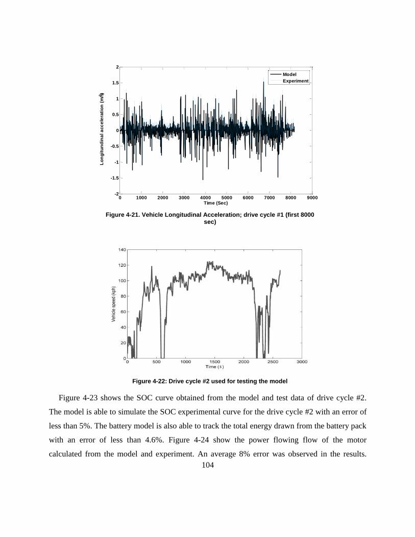
104
Figure 4-21. Vehicle Longitudinal Acceleration; drive cycle #1 (first 8000 sec)
Figure 4-22: Drive cycle #2 used for testing the model
Figure 4-23 shows the SOC curve obtained from the model and test data of drive cycle #2.
The model is able to simulate the SOC experimental curve for the drive cycle #2 with an error of
less than 5%. The battery model is also able to track the total energy drawn from the battery pack
with an error of less than 4.6%. Figure 4-24 show the power flowing flow of the motor
calculated from the model and experiment. An average 8% error was observed in the results.
0 1000 2000 3000 4000 5000 6000 7000 8000 9000-2
-1.5
-1
-0.5
0
0.5
1
1.5
2
Time (Sec)
Lo
ng
itu
nd
ina
l a
cc
ele
rati
on
(m
/s2)
Model
Experiment

105
Figure 4-25 compares the vehicle acceleration from the test data and the model under the test
drive cycle. The model is able to predict the vehicle acceleration with an average 7% error
Table 4-9: Statistics of test drive cycle #2
Cycle duration (sec) 2623
Cycle distance (km) 98.7
Speed (kph) max average
124 84.6
Acceleration (m
s2) 6.44 0.34
Deceleration (m
s2) -5.41 -0.33
Ambient Temperature 2 ℃
Figure 4-23: SOC versus time; obtained from the model and field test related to drive cycle #2.
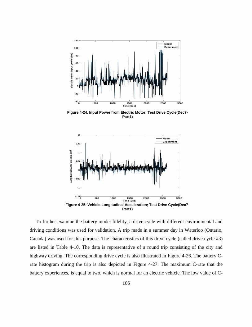
106
Figure 4-24. Input Power from Electric Motor; Test Drive Cycle(Dec7-Part1)
Figure 4-25. Vehicle Longitudinal Acceleration; Test Drive Cycle(Dec7-
Part1)
To further examine the battery model fidelity, a drive cycle with different environmental and
driving conditions was used for validation. A trip made in a summer day in Waterloo (Ontario,
Canada) was used for this purpose. The characteristics of this drive cycle (called drive cycle #3)
are listed in Table 4-10. The data is representative of a round trip consisting of the city and
highway driving. The corresponding drive cycle is also illustrated in Figure 4-26. The battery C-
rate histogram during the trip is also depicted in Figure 4-27. The maximum C-rate that the
battery experiences, is equal to two, which is normal for an electric vehicle. The low value of C-
0 500 1000 1500 2000 2500 3000-40
-20
0
20
40
60
80
100
120
Time (Sec)
Ele
ctr
ic m
oto
r in
pu
t p
ow
er
(kw
)
Model
Experiment
0 500 1000 1500 2000 2500 3000-1.5
-1
-0.5
0
0.5
1
1.5
2
Time (Sec)
Lo
ng
itu
din
al
ac
ce
lera
tio
n (
m/s2
)
Model
Experiment
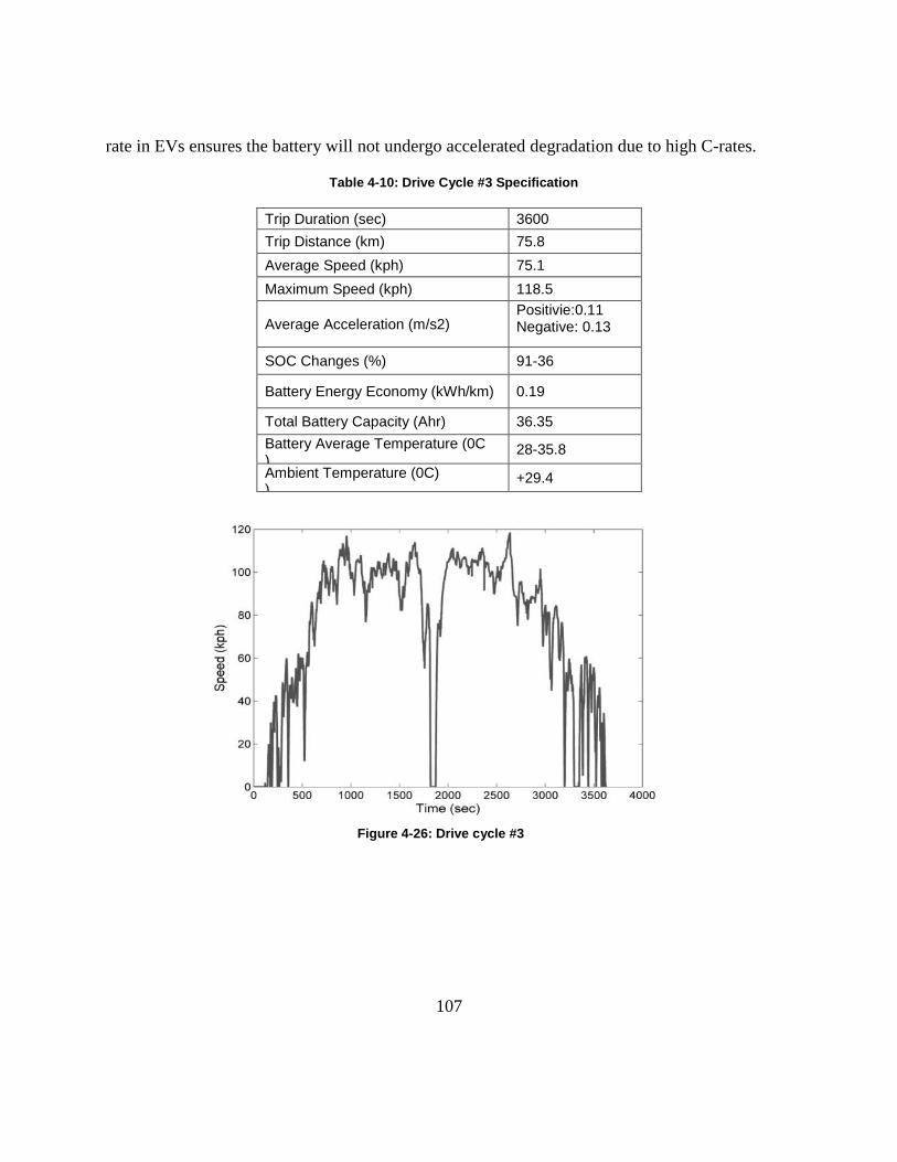
107
rate in EVs ensures the battery will not undergo accelerated degradation due to high C-rates.
Table 4-10: Drive Cycle #3 Specification
Trip Duration (sec) 3600
Trip Distance (km) 75.8
Average Speed (kph) 75.1
Maximum Speed (kph) 118.5
Average Acceleration (m/s2) Positivie:0.11 Negative: 0.13
SOC Changes (%) 91-36
Battery Energy Economy (kWh/km) 0.19
Total Battery Capacity (Ahr) 36.35
Battery Average Temperature (0C )
28-35.8
Ambient Temperature (0C) )
+29.4
Figure 4-26: Drive cycle #3
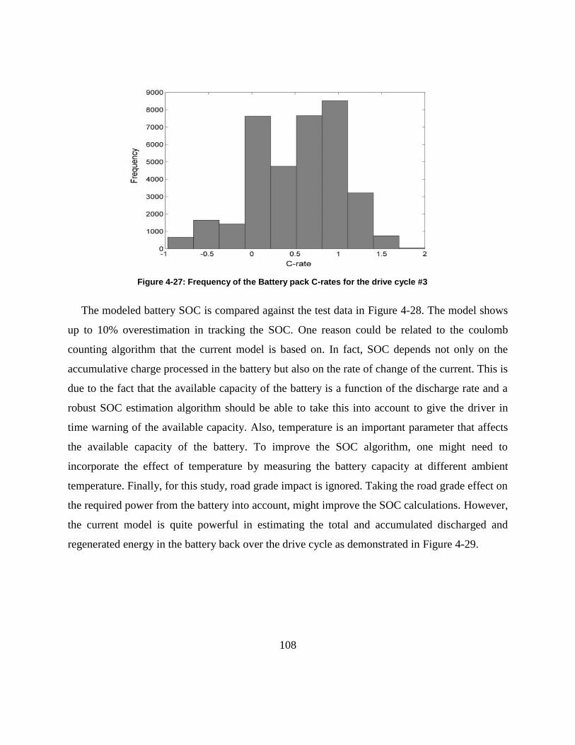
108
Figure 4-27: Frequency of the Battery pack C-rates for the drive cycle #3
The modeled battery SOC is compared against the test data in Figure 4-28. The model shows
up to 10% overestimation in tracking the SOC. One reason could be related to the coulomb
counting algorithm that the current model is based on. In fact, SOC depends not only on the
accumulative charge processed in the battery but also on the rate of change of the current. This is
due to the fact that the available capacity of the battery is a function of the discharge rate and a
robust SOC estimation algorithm should be able to take this into account to give the driver in
time warning of the available capacity. Also, temperature is an important parameter that affects
the available capacity of the battery. To improve the SOC algorithm, one might need to
incorporate the effect of temperature by measuring the battery capacity at different ambient
temperature. Finally, for this study, road grade impact is ignored. Taking the road grade effect on
the required power from the battery into account, might improve the SOC calculations. However,
the current model is quite powerful in estimating the total and accumulated discharged and
regenerated energy in the battery back over the drive cycle as demonstrated in Figure 4-29.

109
Figure 4-28: Battery SOC Validation Against drive cycle #3
Discharged energy Regenerated Energy
Figure 4-29: Battery Model Validation against Test Data over Drive cycle #3
Battery Thermal Behavior
The performance, life, and safety of Li-ion batteries are affected by their operation
temperature. Therefore, for designing the battery pack for EVs, it is important to take into
account the thermal behavior of these batteries. In this section, the thermal behavior of the

110
battery pack based on the field test data and the thermal model developed with consideration of
the effect of the battery reversible and irreversible heat generations is studied. The pack is cooled
by a fan with a flow of air which is assumed to be divided in parallel so that the same amount of
air passes through each module of the pack. Therefore, it is enough to model one single module
to obtain the temperature profile of the whole pack. The cell temperature at each time step is a
function of the generated heat and the rejected heat by forced convection. However the BMS on
this vehicle turns the fan on once the module temperature exceeds 40℃ . Considering the
weather conditions in Waterloo, such a situation rarely happens and therefore it is reasonable to
ignore the forced convection in the battery pack thermal modeling. The heat generation rate
inside the Li-ion cell can be determined from Eq. 2 [26].
��𝑔𝑒𝑛 = ��𝑔𝑒𝑛,reversible + ��𝑔𝑒𝑛,𝑖𝑟reversible = 𝑅𝑖𝑛𝑡𝐼2 + 𝐼𝑇
𝑑(𝑂𝐶𝑉)
𝑑𝑇
(4-3)
Where, Qgen, is the rate of heat generation in the battery pack, I, is the current drawn from the
battery pack, and Rint, is the internal resistant of the battery pack obtained from Eq. 1. In Eq. 2,
the rate of heat generation is expressed as the summation of two terms. The first term represents
the irreversible heat generation, which is always exothermic and the second term is the reversible
heat generation, which can be exothermic or endothermic. In this term, the coefficient of
d(OCV)/dT for a single cell at various SOC are adopted from [48] and plotted in the Figure 4-30.
Figure 4-30: The coefficient of d(OCV)/dT versus SOC for the single cell of the battery back under study [48].
It is noted that this coefficient should be multiplied by the number of series cells in the battery
0 10 20 30 40 50 60 70 80 90 100-4
-2
0
2
4
6
8x 10
-4
SOC (%)
dO
CV
/dT
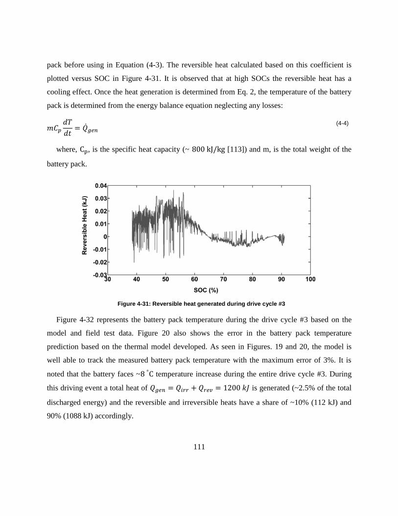
111
pack before using in Equation (4-3). The reversible heat calculated based on this coefficient is
plotted versus SOC in Figure 4-31. It is observed that at high SOCs the reversible heat has a
cooling effect. Once the heat generation is determined from Eq. 2, the temperature of the battery
pack is determined from the energy balance equation neglecting any losses:
𝑚𝐶𝑝𝑑𝑇
𝑑𝑡= ��𝑔𝑒𝑛
(4-4)
where, Cp, is the specific heat capacity (~ 800 kJ/kg [113]) and m, is the total weight of the
battery pack.
Figure 4-31: Reversible heat generated during drive cycle #3
Figure 4-32 represents the battery pack temperature during the drive cycle #3 based on the
model and field test data. Figure 20 also shows the error in the battery pack temperature
prediction based on the thermal model developed. As seen in Figures. 19 and 20, the model is
well able to track the measured battery pack temperature with the maximum error of 3%. It is
noted that the battery faces ~8 °C temperature increase during the entire drive cycle #3. During
this driving event a total heat of 𝑄𝑔𝑒𝑛 = 𝑄𝑖𝑟𝑟 + 𝑄𝑟𝑒𝑣 = 1200 𝑘𝐽 is generated (~2.5% of the total
discharged energy) and the reversible and irreversible heats have a share of ~10% (112 kJ) and
90% (1088 kJ) accordingly.

112
Figure 4-32: Validation of the battery pack thermal model for drive cycle #3.
Figure 4-33: Modeling error in predicting the battery pack temperature over drive cycle #3
4.3.3 Case study- Testing the proposed ECM with a Real-life drive cycle
In this section, performance of the proposed ECM in Chapter 3 is evaluated with a real-life
drive cycle (drive cycle #3-Figure 4-26). For this purpose, it is assumed that the battery pack on
the research EV is comprised of the battery cells for which the ECM was developed. As these
cells are different from the original battery cells on the research EV (cylindrical Valence
batteries, LiFeMgPO4) in terms of geometry and chemistry, a different thermo-electrical
performance would be expected from the new battery pack. Therefore, the first step in this
analysis would be scaling the battery current profile according to the specifications of the new
battery cells.
The cells arrangement in the new pack is assumed to be 3𝑝 × 105𝑠. As the vehicle dynamics
and power demand over the test drive cycle remains the same, the new battery pack would have
to provide the same power requirement (but a different current and voltage profile). Afterwards,
the Autonomie model of the vehicle has to be modified to take the power profile as the input. It
is worth to mention that in Autonomie, the input is the drive cycle and based on the
instantaneous difference between the actual speed and the desired speed, a PI controller
determines the adjustments to the torque demand signal in the driver sub-model. Therefore, for
the current analysis, the controller (in the driver sub-model) was modified to take the battery

113
power difference as its decision criteria. Also, the PI controller was upgraded to a PID controller
to increase the accuracy of the model in following the power profile fluctuation as shown in
Appendix C. the simulated battery power is plotted against the experimental data in Figure 4-34.
An average error of 5% was observed in the simulated power profiles.
Figure 4-34 Battery power profiles under test drive cycle operation
The resulting current profile is shown in Figure 4-35
Figure 4-35 Profile of battery current of the drive cycle #3
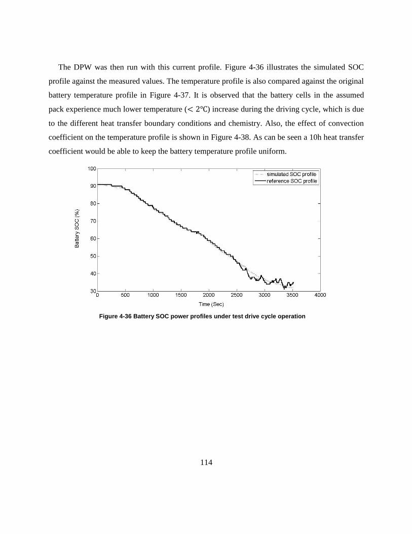
114
The DPW was then run with this current profile. Figure 4-36 illustrates the simulated SOC
profile against the measured values. The temperature profile is also compared against the original
battery temperature profile in Figure 4-37. It is observed that the battery cells in the assumed
pack experience much lower temperature (< 2℃) increase during the driving cycle, which is due
to the different heat transfer boundary conditions and chemistry. Also, the effect of convection
coefficient on the temperature profile is shown in Figure 4-38. As can be seen a 10h heat transfer
coefficient would be able to keep the battery temperature profile uniform.
Figure 4-36 Battery SOC power profiles under test drive cycle operation

115
Figure 4-37 Profile of battery temperature during the tests drive cycle
Figure 4-38 Tests drive cycle and relevant battery performance profiles
4.3.4 Overall Powertrain Efficiency of EV-ACX2.5
To evaluate the overall powertrain efficiency of the EV-ACX2.5 vehicle, the efficiency of
each component must be first calculated. The main components involved in vehicle energy
conversion, from the wall to the wheel, are the charging station, AC/DC convertor (on-board
vehicle charger), the vehicle battery, and the electric traction motor. The efficiency of each
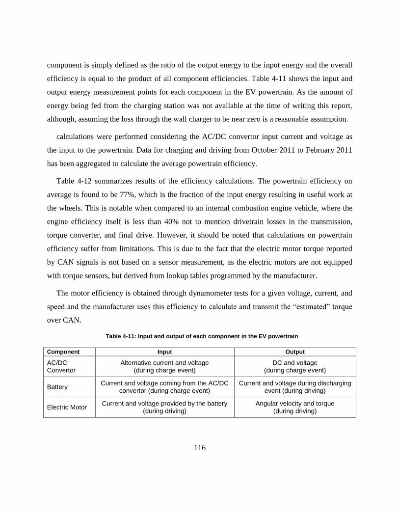
116
component is simply defined as the ratio of the output energy to the input energy and the overall
efficiency is equal to the product of all component efficiencies. Table 4-11 shows the input and
output energy measurement points for each component in the EV powertrain. As the amount of
energy being fed from the charging station was not available at the time of writing this report,
although, assuming the loss through the wall charger to be near zero is a reasonable assumption.
calculations were performed considering the AC/DC convertor input current and voltage as
the input to the powertrain. Data for charging and driving from October 2011 to February 2011
has been aggregated to calculate the average powertrain efficiency.
Table 4-12 summarizes results of the efficiency calculations. The powertrain efficiency on
average is found to be 77%, which is the fraction of the input energy resulting in useful work at
the wheels. This is notable when compared to an internal combustion engine vehicle, where the
engine efficiency itself is less than 40% not to mention drivetrain losses in the transmission,
torque converter, and final drive. However, it should be noted that calculations on powertrain
efficiency suffer from limitations. This is due to the fact that the electric motor torque reported
by CAN signals is not based on a sensor measurement, as the electric motors are not equipped
with torque sensors, but derived from lookup tables programmed by the manufacturer.
The motor efficiency is obtained through dynamometer tests for a given voltage, current, and
speedandthemanufacturerusesthisefficiencytocalculateandtransmitthe“estimated”torque
over CAN.
Table 4-11: Input and output of each component in the EV powertrain
Component Input Output
AC/DC Convertor
Alternative current and voltage (during charge event)
DC and voltage (during charge event)
Battery Current and voltage coming from the AC/DC
convertor (during charge event) Current and voltage during discharging
event (during driving)
Electric Motor Current and voltage provided by the battery
(during driving) Angular velocity and torque
(during driving)

117
Table 4-12: Monthly efficiency of the EV-ACX2.5 powertrain
Month AC/DC convertor
Efficiency (%)
Battery
Efficiency (%)
Electric Motor
Efficiency (%)
Overall efficiency
(%) October, 2011 91.36 98 87 78
November, 2011 91.37 97 85 75.3
December, 2011 91.39 99 85.4 77
January, 2012 91.36 99 87 78
February, 2012 91.37 98 86.2 77.1
4.3.5 Energy Requirement of EV-ACX2.5 as a Fleet Vehicle
To perform a more in-depth comparison between EV-ACX2.5 and fleet performance, the EV
PSAT model was runthroughallof thecollected‘HEV‘drivecyclesfromHEVvehiclesover
three months (November, December, January) to yield the amount of energy required as if the
EV was used as a fleet vehicle by Burlington Hydro. For this purpose, first the HEV drive cycles
were defined and saved as velocity-time data sheets; afterwards a script written in Matlab called
and ran the PSAT model for each of the drive cycles and updated the consumed energy value
accordingly. Results are shown in Table 4-13. The results are based on the assumption that the
battery was fully charged at the beginning of each trip. The consumed energy reported in
Table 4-13 is calculated by integrating instantaneous power drawn from the battery (as was
simulated by PSAT) over each trip. On average, the EV-ACX2.5 is able to complete all of the
HEV cycles using only 60% of the energy used by the HEV. This is equal to a 64% cost saving
as is represented in Table 4-14. The cost of HEV fuelling is calculated based on average monthly
price of gas in Burlington-Hamilton area [106]. It is also of interest to perform a well-to-wheel
life cycle analysis and compare the emissions of the EV with the HEV. For this purpose a
validated model of the HEV needs to be developed. This task can be considered for future
analysis.
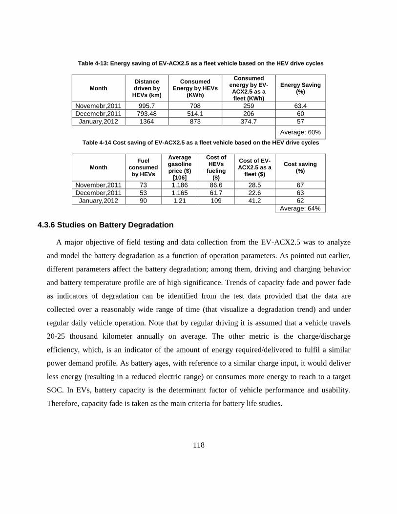
118
Table 4-13: Energy saving of EV-ACX2.5 as a fleet vehicle based on the HEV drive cycles
Month Distance driven by
HEVs (km)
Consumed Energy by HEVs
(KWh)
Consumed energy by EV-ACX2.5 as a fleet (KWh)
Energy Saving (%)
Novemebr,2011 995.7 708 259 63.4
Decemebr,2011 793.48 514.1 206 60
January,2012 1364 873 374.7 57
Average: 60%
Table 4-14 Cost saving of EV-ACX2.5 as a fleet vehicle based on the HEV drive cycles
Month Fuel
consumed by HEVs
Average gasoline price ($)
[106]
Cost of HEVs
fueling ($)
Cost of EV-ACX2.5 as a
fleet ($)
Cost saving (%)
November,2011 73 1.186 86.6 28.5 67
December,2011 53 1.165 61.7 22.6 63
January,2012 90 1.21 109 41.2 62
Average: 64%
4.3.6 Studies on Battery Degradation
A major objective of field testing and data collection from the EV-ACX2.5 was to analyze
and model the battery degradation as a function of operation parameters. As pointed out earlier,
different parameters affect the battery degradation; among them, driving and charging behavior
and battery temperature profile are of high significance. Trends of capacity fade and power fade
as indicators of degradation can be identified from the test data provided that the data are
collected over a reasonably wide range of time (that visualize a degradation trend) and under
regular daily vehicle operation. Note that by regular driving it is assumed that a vehicle travels
20-25 thousand kilometer annually on average. The other metric is the charge/discharge
efficiency, which, is an indicator of the amount of energy required/delivered to fulfil a similar
power demand profile. As battery ages, with reference to a similar charge input, it would deliver
less energy (resulting in a reduced electric range) or consumes more energy to reach to a target
SOC. In EVs, battery capacity is the determinant factor of vehicle performance and usability.
Therefore, capacity fade is taken as the main criteria for battery life studies.
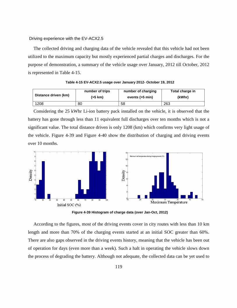
119
Driving experience with the EV-ACX2.5
The collected driving and charging data of the vehicle revealed that this vehicle had not been
utilized to the maximum capacity but mostly experienced partial charges and discharges. For the
purpose of demonstration, a summary of the vehicle usage over January, 2012 till October, 2012
is represented in Table 4-15.
Table 4-15 EV-ACX2.5 usage over January 2012- October 19, 2012
Distance driven (km) number of trips
(>5 km)
number of charging
events (>5 min)
Total charge in
(kWhr)
1208 80 58 263
Considering the 25 kWhr Li-ion battery pack installed on the vehicle, it is observed that the
battery has gone through less than 11 equivalent full discharges over ten months which is not a
significant value. The total distance driven is only 1208 (km) which confirms very light usage of
the vehicle. Figure 4-39 and Figure 4-40 show the distribution of charging and driving events
over 10 months.
Figure 4-39 Histogram of charge data (over Jan-Oct, 2012)
According to the figures, most of the driving events cover in city routes with less than 10 km
length and more than 70% of the charging events started at an initial SOC greater than 60%.
There are also gaps observed in the driving events history, meaning that the vehicle has been out
of operation for days (even more than a week). Such a halt in operating the vehicle slows down
the process of degrading the battery. Although not adequate, the collected data can be yet used to
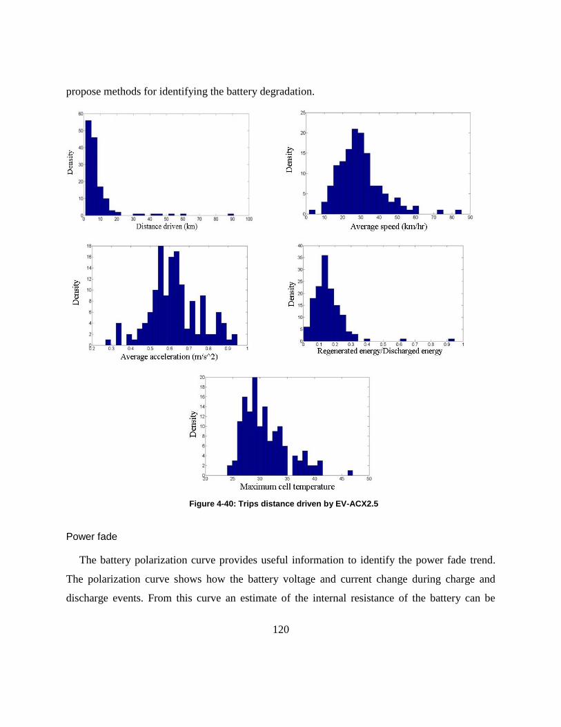
120
propose methods for identifying the battery degradation.
Figure 4-40: Trips distance driven by EV-ACX2.5
Power fade
The battery polarization curve provides useful information to identify the power fade trend.
The polarization curve shows how the battery voltage and current change during charge and
discharge events. From this curve an estimate of the internal resistance of the battery can be

121
obtained; internal resistance is the parameter that directly represents the power-fade inside the
battery. It is expected that after a sufficiently large time period, the polarization curve slope will
change and show a growth in internal resistance. In order to investigate how the battery internal
resistance has changed over one year of operation, data from three drive cycles driven on
November 25, 2011, December 7, 2011 and October 05, 2012 have been used to generate the
polarization curve by making scatter plots of voltage versus charge processed (Figure 4-41) and
fitting a polynomial curve. The average battery temperature range was 20-35 ºC for the
November 25 drive cycle, 20-47 ºC for October 5 and 15-38 ºC for December 7. The high
temperature changes in the December 7 and November 25 drive cycles are due to the aggressive
driving, which results in higher discharge currents and heat generation as well. As shown in
Figure 4-42 as the battery ages, its polarization curve will have a greater slope, i.e. for the same
amount of charge processed, the battery will experience a higher voltage decrease. Also, the
highest discrepancy in the fitted voltage profile was observed to be at 63 Ahr (~ 90% DOD)
showing 6% increase in the bulk internal resistance.
However, care should be taken when interpreting such polarization curves; because the
polarization not only depends on the battery SOH, but also on the battery operating temperature.
Therefore, unless one could differentiate the temperature and SOH impacts on the polarization
curve, the observed decrease in the voltage could not be solely translated as resistance increase in
the battery. Therefore, to enable a comparison of battery polarization curves that yields an
indication of power fade, the test data should be collected from trips with identical battery
operating temperatures. Again, dynamometer testing in a controlled environment is much
preferred for this purpose. Other option is implementing an active thermal management for the
battery pack which is able to keep the battery temperature in a narrow operating range. In
addition, driving behavior which directly affects the current demand from the battery is the other
significant parameter on the polarization curve. For a reasonable comparison, polarization curves
over similar driving events (in terms of average and maximum speed and acceleration) should be
compared against each other.

122
Figure 4-41 selected drive cycles for comparing the polarization curves
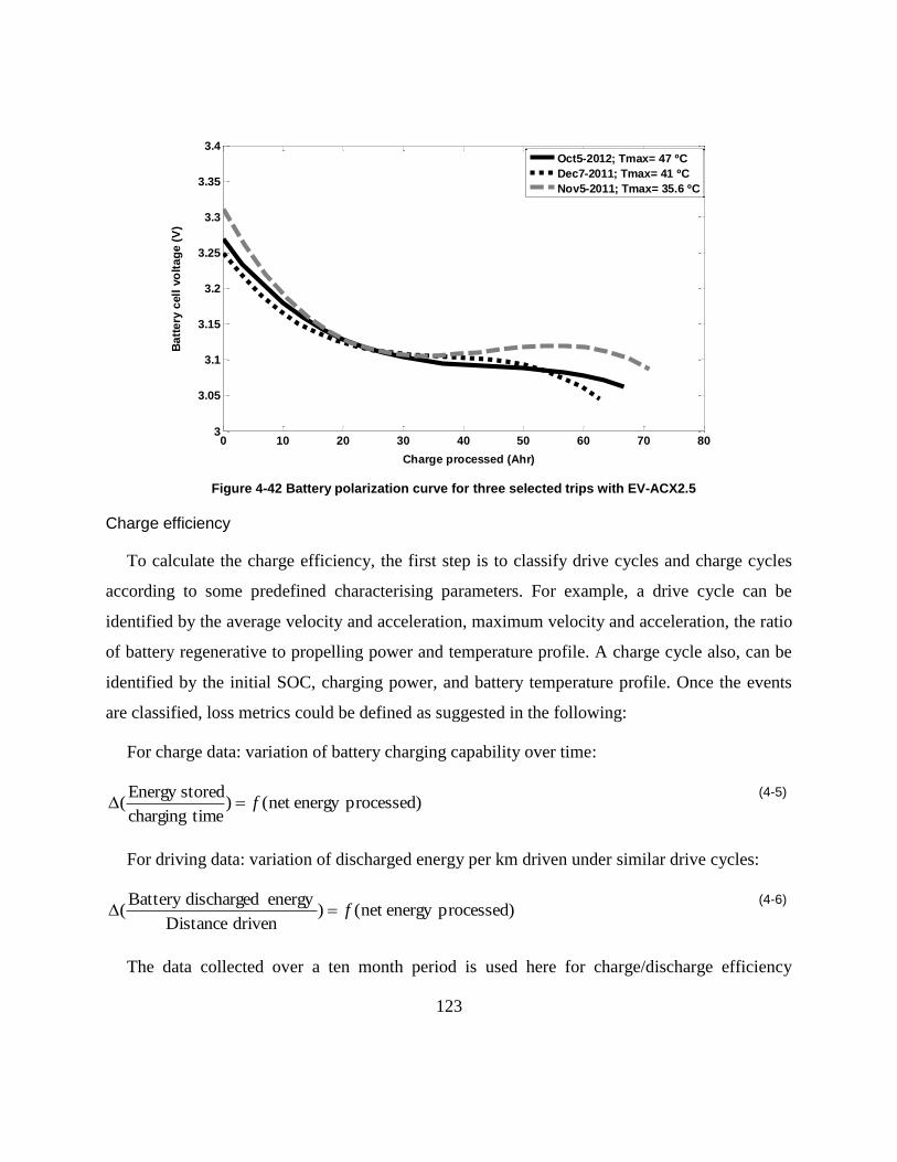
123
Figure 4-42 Battery polarization curve for three selected trips with EV-ACX2.5
Charge efficiency
To calculate the charge efficiency, the first step is to classify drive cycles and charge cycles
according to some predefined characterising parameters. For example, a drive cycle can be
identified by the average velocity and acceleration, maximum velocity and acceleration, the ratio
of battery regenerative to propelling power and temperature profile. A charge cycle also, can be
identified by the initial SOC, charging power, and battery temperature profile. Once the events
are classified, loss metrics could be defined as suggested in the following:
For charge data: variation of battery charging capability over time:
processed)energy net ()timecharging
storedEnergy( f
(4-5)
For driving data: variation of discharged energy per km driven under similar drive cycles:
)processedenergy net ()drivenDistance
energydischargedBattery( f
(4-6)
The data collected over a ten month period is used here for charge/discharge efficiency
0 10 20 30 40 50 60 70 803
3.05
3.1
3.15
3.2
3.25
3.3
3.35
3.4
Charge processed (Ahr)
Ba
tte
ry c
ell
vo
lta
ge
(V
)
Oct5-2012; Tmax= 47 ºC
Dec7-2011; Tmax= 41 ºC
Nov5-2011; Tmax= 35.6 ºC

124
analysis. Constraints for extracting similar charge and driving data are presented in Table 4-14.
Similar charge and driving events extracted accordingly are illustrated in Figure 4-43 and
Figure 4-44. It is expected to see a decreasing trend in both figures (as discussed earlier).
Figure 4-44 shows an overall decrease, however, due to the limited data points used for
classification and measurement error this trend is not very obvious in these plots. A large data
pool (over a time span of 2-3 years) should result in the expected trend.
Table 4-16 Extraction of similar charge and driving events
charge driving
Range
observed
Maximum cell temperature: 19ᵒC-43ᵒC Initial SOC: 1%-99%
maximum cell temperature: 24ᵒC-47ᵒC Average speed: 5-85 (kph Average positive acceleration: 0.95 −
0.27 (𝑚
𝑠2)
Regenerative to discharged energy ratio: 0.0037-0.95
Selected
range
Maximum temperature: 28ᵒC -35 ᵒC Initial SOC: 80%-90%
Maximum temperature: 26ᵒC -32 ᵒC Average speed: 25-30 (kph)
Average acceleration: 0.5-0.7 (𝑚
𝑠2)
Regenerative energy to discharged energy: 0.08-0.13
Figure 4-43 Charge input over time for 10 similar charging events
1 2 3 4 5 6 7 8 9 102.6
2.8
3
3.2
3.4
3.6
Charge event
Ch
arg
ed
en
erg
y/T
ime
(k
W)
-85.28 kWhr
+77.82 kWhr
-5.22 kWhr
+1.1 kWhr-20.93 kWhr
+18.73 kWhr-7.95kWhr
+4.52 kWhr
-13.06 kWhr
+3.7 kWhr-31.8 kWhr
+25.75 kWhr
-8.2 kWhr
+4.76 kWhr-17.3 kWhr
+13.36 kWhr
July,2012,
Tmax=29
SOC=83
-5.63 kWhr
+0.96 kWhr
May,2012,
Tmax=30
SOC=87
Mar,2012,
Tmax=31
SOC=84
Jan,2012,
Tmax=29
SOC=82
Jan,2012,
Tmax=31
SOC=87
June,2012,
Tmax=34
SOC=81
Aug,2012,
Tmax=34
SOC=88
June,2012,
Tmax=33
SOC=89
June,2012,
Tmax=33
SOC=82
July,2012,
Tmax=34
SOC=85

125
Figure 4-44 Energy discharged per km driven for 6 similar driving events
Considerations- With this suggestion it is assumed that the SOC reported on the CAN is
calculated based on an adaptive algorithm which is able to incorporate the effect of different
parameters on capacity (such as discharging rate and temperature). However, there are always
uncertainties with the road test data as there is no control on the weather conditions and traffic
(such as stops at red lights), it is not possible to drive exactly the same trips and evaluate the
capacity trends. To get the most accurate determination of capacity fade, it is necessary to run
capacity measurement experiments in a controlled environment. A test station could be
developed to enable cycling the battery under a set of pre-defined duty cycles allowing better
observation of the capacity degradation.
Capacity Fade
In order to calculate the capacity fade it is required that a baseline capacity value be
established when the battery is new, and that a standard procedure be developed for measuring
the capacity of the battery as time progresses. The suggested method for measuring the battery
capacity on vehicle is as following:
1 2 3 4 5 60.18
0.2
0.22
0.24
0.26
0.28
0.3
0.32
Driving event
Dis
ch
arg
ed
en
erg
y/ d
ista
nc
e (
kW
hr/
km
)
Mar 13, 2012
Tmax=29
dist=4.25 km
Jan 15, 2012
Tmax=29
dist=4.65 km
Mar 2, 2012
Tmax=26
dist=4.62 km
June 8, 2012
Tmax=31
dist=6.97 km
June 26, 2012
Tmax=32
dist=7.4 km
June 13, 2012
Tmax=31
dist=6.15 km
- 59.8 kWhr
+62.5 kWhr-35.8 kWhr
+36.3 kWhr- 9.87 kWhr
+6.02 kWhr
- 30.72 kWhr
+29.93 kWhr
- 34.12 kWhr
+36.6 kWhr
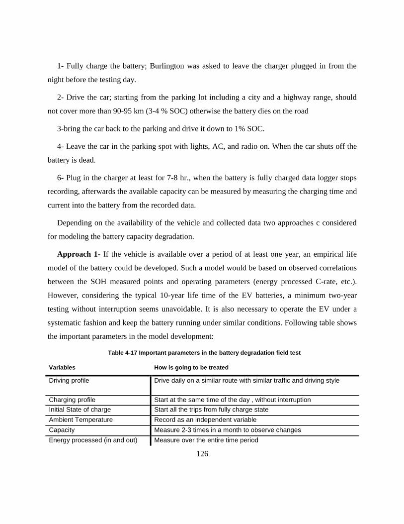
126
1- Fully charge the battery; Burlington was asked to leave the charger plugged in from the
night before the testing day.
2- Drive the car; starting from the parking lot including a city and a highway range, should
not cover more than 90-95 km (3-4 % SOC) otherwise the battery dies on the road
3-bring the car back to the parking and drive it down to 1% SOC.
4- Leave the car in the parking spot with lights, AC, and radio on. When the car shuts off the
battery is dead.
6- Plug in the charger at least for 7-8 hr., when the battery is fully charged data logger stops
recording, afterwards the available capacity can be measured by measuring the charging time and
current into the battery from the recorded data.
Depending on the availability of the vehicle and collected data two approaches c considered
for modeling the battery capacity degradation.
Approach 1- If the vehicle is available over a period of at least one year, an empirical life
model of the battery could be developed. Such a model would be based on observed correlations
between the SOH measured points and operating parameters (energy processed C-rate, etc.).
However, considering the typical 10-year life time of the EV batteries, a minimum two-year
testing without interruption seems unavoidable. It is also necessary to operate the EV under a
systematic fashion and keep the battery running under similar conditions. Following table shows
the important parameters in the model development:
Table 4-17 Important parameters in the battery degradation field test
Variables How is going to be treated
Driving profile Drive daily on a similar route with similar traffic and driving style
Charging profile Start at the same time of the day , without interruption
Initial State of charge Start all the trips from fully charge state
Ambient Temperature Record as an independent variable
Capacity Measure 2-3 times in a month to observe changes
Energy processed (in and out) Measure over the entire time period
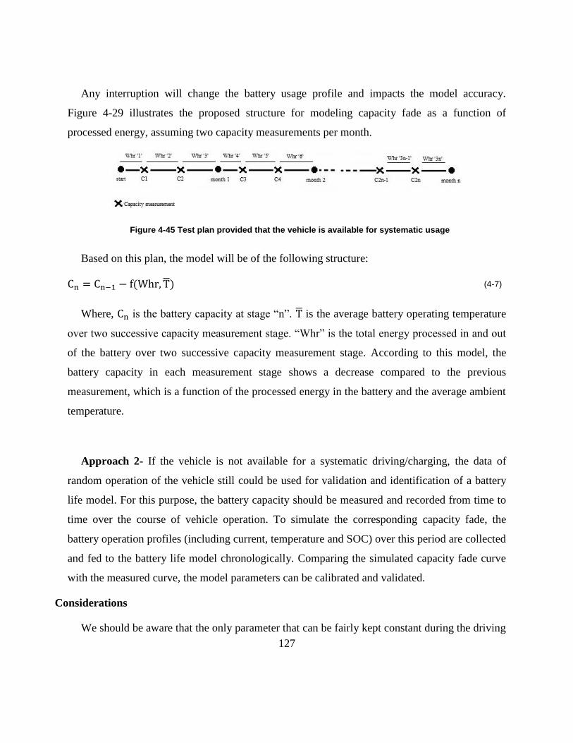
127
Any interruption will change the battery usage profile and impacts the model accuracy.
Figure 4-29 illustrates the proposed structure for modeling capacity fade as a function of
processed energy, assuming two capacity measurements per month.
Figure 4-45 Test plan provided that the vehicle is available for systematic usage
Based on this plan, the model will be of the following structure:
Cn = Cn−1 − f(Whr, T) (4-7)
Where, Cn isthebatterycapacityatstage“n”.T is the average battery operating temperature
overtwosuccessivecapacitymeasurementstage.“Whr”isthetotalenergyprocessedinandout
of the battery over two successive capacity measurement stage. According to this model, the
battery capacity in each measurement stage shows a decrease compared to the previous
measurement, which is a function of the processed energy in the battery and the average ambient
temperature.
Approach 2- If the vehicle is not available for a systematic driving/charging, the data of
random operation of the vehicle still could be used for validation and identification of a battery
life model. For this purpose, the battery capacity should be measured and recorded from time to
time over the course of vehicle operation. To simulate the corresponding capacity fade, the
battery operation profiles (including current, temperature and SOC) over this period are collected
and fed to the battery life model chronologically. Comparing the simulated capacity fade curve
with the measured curve, the model parameters can be calibrated and validated.
Considerations
We should be aware that the only parameter that can be fairly kept constant during the driving

128
is the drive cycle (v-t) profile but not the C-rate profiles. The reason is that as the battery ages,
more energy will be wasted as heat (due to resistance growth) and therefore to cover a similar
driving distance more energy would be discharged from the battery in total, and, the c-rate
profile would also change over time.
Also, SOH measurement itself impacts the battery health. When running life tests in the lab,
the degradation effects associated with SOH (capacity) test is minimized by using a very low C-
rate profile to the battery. In case of field testing, two solutions can be considered: 1) running the
vehicle with very low c-rates (e.g. 10-15 kph) and cycle the battery down to zero percent SOC,
which is a time consuming procedure. 2) Minimize the frequency of SOH measurement tests; to
limit the number of full discharge & charge cycles minimize the SOH test impacts. But, from the
modeling aspect, decreasing the number of SOH tests results in a less reliable model
development as fewer response points will be available.
It should be noted that a model described in the approach 1 would be valid for only one
specific duty cycle. As there are infinite combinations of driving and charging profiles possible
in reality, it would be best to employ multiple test vehicles, each with a different duty cycle.
Due to the technical issues, the vehicle operation was interrupted several times during the
course of the project. Also, as the operation data histogram showed, the vehicle was not used
very much by the company staff. Therefore, it was decided to bring the vehicle to Waterloo and
drive it in a daily fashion. A route containing in-city and highway driving as presented earlier in
Figure 4-26 was chosen for this purpose and two graduate students involved in the project drove
the vehicle every day. After each driving, the vehicle was taken to the charge station for a full
recharge and finally back to the parking lot for the next day driving. The tests were repeated
every day for four months until again the vehicle went inoperable and tests were halted. During
the test period, the battery capacity was measured and recorded twice a month (~ every 15 days).
Results of capacity tests over four months of continuous test are presented in Table 4-18 and
plotted in Figure 4-46. As in real life vehicle operation, the current profile is continuously
changing; it makes more sense to express the battery capacity in terms of the capability in
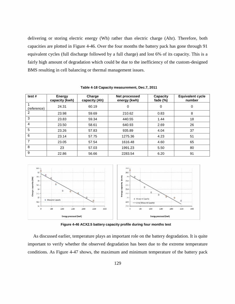
129
delivering or storing electric energy (Wh) rather than electric charge (Ahr). Therefore, both
capacities are plotted in Figure 4-46. Over the four months the battery pack has gone through 91
equivalent cycles (full discharge followed by a full charge) and lost 6% of its capacity. This is a
fairly high amount of degradation which could be due to the inefficiency of the custom-designed
BMS resulting in cell balancing or thermal management issues.
Table 4-18 Capacity measurement, Dec.7, 2011
test # Energy capacity (kwh)
Charge capacity (Ah)
Net processed energy (kwh)
Capacity fade (%)
Equivalent cycle number
1 (reference)
24.31 60.19 0 0 0
2 23.98 59.69 210.62 0.83 8
3 23.83 59.34 440.55 1.44 18
4 23.50 58.61 640.93 2.69 26
5 23.26 57.83 935.89 4.04 37
6 23.14 57.75 1275.36 4.23 51
7 23.05 57.54 1616.48 4.60 65
8 23 57.03 1991.23 5.50 80
9 22.86 56.66 2283.54 6.20 91
Figure 4-46 ACX2.5 battery capacity profile during four months test
As discussed earlier, temperature plays an important role on the battery degradation. It is quite
important to verify whether the observed degradation has been due to the extreme temperature
conditions. As Figure 4-47 shows, the maximum and minimum temperature of the battery pack

130
over the four months of testing is mostly in the range of 10ᵒC-35ᵒC which is a modest range and
does not impose accelerated degradation. Therefore, the observed degradation could be attributed
to normal cycling and a life model could be calibrated accordingly.
Figure 4-47 Battery pack maximum and minimum temperature during each event (Over July-October)
Battery Degradation Modeling and calibration
To model the battery degradation over a drive cycles or charge cycles, a life model is required
which is able to capture the effect of different variables such as SOC, C-rate, temperature. The
extendedNing’smodelprovides such capabilities and was used for the current studies.Ning’s
model models the higher currents present in vehicle powertrain applications, and also takes into
account the degradation under constant voltage charging operation [114]. Ning’s model
incorporates porous electrode theory, concentrated solution theory, Ohm’s law,
intercalation/deintercalation kinetics, and transport in both the solid phase and electrolyte phase
[114]:
𝑗𝑝𝑎𝑟𝑎 = 𝑗𝑝𝑎𝑟𝑎0 𝑒𝑥𝑝 (
𝛼𝑐𝐹
𝑅𝑇𝜂)
(4-8)
Where, 𝑗𝑝𝑎𝑟𝑎, is the local parasitic reaction current density. More details about this model can
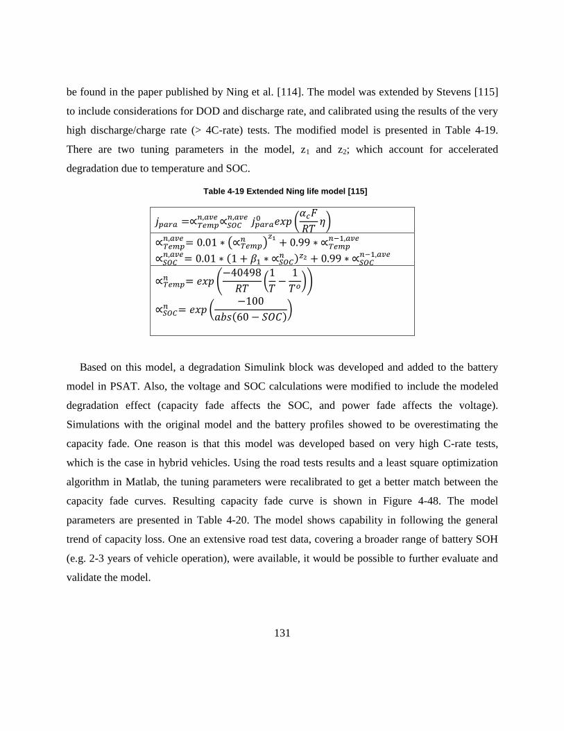
131
be found in the paper published by Ning et al. [114]. The model was extended by Stevens [115]
to include considerations for DOD and discharge rate, and calibrated using the results of the very
high discharge/charge rate (> 4C-rate) tests. The modified model is presented in Table 4-19.
There are two tuning parameters in the model, z1 and z2; which account for accelerated
degradation due to temperature and SOC.
Table 4-19 Extended Ning life model [115]
𝑗𝑝𝑎𝑟𝑎 =∝𝑇𝑒𝑚𝑝𝑛,𝑎𝑣𝑒∝𝑆𝑂𝐶
𝑛,𝑎𝑣𝑒 𝑗𝑝𝑎𝑟𝑎0 𝑒𝑥𝑝 (
𝛼𝑐𝐹
𝑅𝑇𝜂)
∝𝑇𝑒𝑚𝑝𝑛,𝑎𝑣𝑒= 0.01 ∗ (∝𝑇𝑒𝑚𝑝
𝑛 )𝑧1+ 0.99 ∗ ∝𝑇𝑒𝑚𝑝
𝑛−1,𝑎𝑣𝑒
∝𝑆𝑂𝐶𝑛,𝑎𝑣𝑒= 0.01 ∗ (1 + 𝛽1 ∗ ∝𝑆𝑂𝐶
𝑛 )𝑧2 + 0.99 ∗ ∝𝑆𝑂𝐶𝑛−1,𝑎𝑣𝑒
∝𝑇𝑒𝑚𝑝𝑛 = 𝑒𝑥𝑝 (
−40498
𝑅𝑇(1
𝑇−1
𝑇𝑜))
∝𝑆𝑂𝐶𝑛 = 𝑒𝑥𝑝 (
−100
𝑎𝑏𝑠(60 − 𝑆𝑂𝐶))
Based on this model, a degradation Simulink block was developed and added to the battery
model in PSAT. Also, the voltage and SOC calculations were modified to include the modeled
degradation effect (capacity fade affects the SOC, and power fade affects the voltage).
Simulations with the original model and the battery profiles showed to be overestimating the
capacity fade. One reason is that this model was developed based on very high C-rate tests,
which is the case in hybrid vehicles. Using the road tests results and a least square optimization
algorithm in Matlab, the tuning parameters were recalibrated to get a better match between the
capacity fade curves. Resulting capacity fade curve is shown in Figure 4-48. The model
parameters are presented in Table 4-20. The model shows capability in following the general
trend of capacity loss. One an extensive road test data, covering a broader range of battery SOH
(e.g. 2-3 years of vehicle operation), were available, it would be possible to further evaluate and
validate the model.

132
Figure 4-48 Simulated capacity fade using the calibrated life model
Table 4-20 Model parameters calibrated with road test data
Parameter Value
β1 2
Z1 0.1
Z2 2
Jopara 8x10
-9
αc 0.5
4.4 Conclusion
In this chapter, results of Li-ion battery field test were presented. A converted Ford Escape
powered by Li-ion battery packs was instrumented by a data logger and the powertrain and
battery data under driving and charging was collected through the CANBus. A model of the EV
powertrain was developed in PSAT and calibrated based on the road test data. The battery OCV
and internal resistance were estimated and a simple battery model including a voltage source and
charge/discharge resistance was developed accordingly. It was shown that the battery OCV can
be estimated with an acceptable accuracy from the driving data. The model was then validated
against several drive cycles and profiles of SOC, charge and discharge energy and battery
temperature were nicely compared with the experimental data. The reversible heat showed to
have a portion of 10% in the total heat during a sample driving event in a summer day. The

133
collected data from the EV were also used to identify the degradation trend sin the battery.
Power fade, capacity fades and charge efficiency were studied through the data as three
degradation metrics. A battery life model was also calibrated using the observed capacity
degradation over a four-month testing period. Validation of the model will be possible once more
data points are available. It was initially intended to develop an empirical life model of the
battery. Due to the limited data, the degradation study did not meet its targeted goal. However,
sample analysis was presented as a pathway for future studies.
134
Chapter 5
Modeling of Battery Lifetime in Hybrid
Vehicle Operation
This chapter presents a study on the Li-ion battery operation in a PHEV through simulations.
The objective is to evaluate impacts of climate control load as well as thermal preconditioning of
the battery under different drive cycles on the vehicle range and battery life.
The following section is mainly based on the paper titled “Evaluation of Air Conditioning
Impact on the Electric Vehicle Range and Li-Ion Battery Life” by“Samadani et.al”published by
the Society of automotive Engineer (SAE). This thesis author specific contribution to this paper
is to: “conduct the modeling, prepare the graphics and results and the final manuscript. This
paper is co-authored by Dr. Fowler and Dr. Fraser as supervisors.
5.1 Range Anxiety and Auxiliary loads in PEVs
HEVs have already been introduced into the market as an alternative to conventional vehicles.
However, to move away from fossil fuel energy sources, a demand for PHEV systems with all-
electric range (AER) is increasing [116]. However, when it comes to making a purchase
decision, consumers express concerns; anxiety about the range capability of the EVs (especially
in harsh climates) besides initial costs and charging issues lies on the top of the list. The range of
an EV or charge depleting range (CD) in a PHEV, is limited by the available capacity of the on-
board battery, and directly related to the battery size and restricted by the vehicle weight and cost
constraints.
In this regard, climate control loads are known to strongly aggravate the EV range. In a PHEV
equipped with electric climate control system, the battery provides the driving power as well as
auxiliary loads demands. The vehicle climate control system, i.e. air conditioning (A/C) and

135
heating, is responsible for providing sufficient thermal loads to quickly regulate a comfortable
cabin temperature requested by the vehicle occupants. Such requirement would be more critical
in case the vehicle has passed a period of hot or cold thermal soak. A/C is believed to be the
main accessory requiring the largest quantity of power from the traction source resulting in a
reduced AER and increased dependence on fossil fuel. It is reported that in an EV, A/C may
reduce the driving range up to 35%, depending on the AC usage frequency [37]. Associated with
the charge-depleting (CD) range reduction, there would be increased battery wear for the same
distance driven when AC/heater system is operating, thanks to the higher C-rates imposed on the
battery. As a solution, thermal preconditioning of the cabin and battery using off-board power
(e.g. grid power) has been introduced to alleviate these impacts [117]. Regulating the battery
initial temperature and reducing the higher transient thermal loads, preconditioning also helps the
battery operate in its optimum temperature range (~20-35ᵒC) and yield best capacity and power
performance [95], which would result in an optimized battery life and AER.
In this chapter, EV range capability, and battery performance and life of a PHEV are studied
under different climate scenarios and operating conditions. A thermal model of cabin
temperature is developed that simulates the interior temperature profile of the cabin. The model
incorporates the ambient conditions, solar load, and the vehicle speed and is able to predict the
required cooling (heating) load to cool down (warm up) the cabin from an initial state to a
desired state. A model of a series PHEV and a parallel PHEV developed in Autonomie are used
for the simulations. The thermal model is coupled with the vehicle models to yield the battery
SOC at the end of the simulation, resulting AER and battery life degradation.
5.2 Cabin Thermal Model
To estimate the extra power required by the AC (heating) system, first the temperature profile
of the cabin during a driving event needs to be determined. Therefore, a thermal model of the
cabin was developed. The model incorporates the effect of solar radiation on the outer surface of
the vehicle body, forced convection between the ambient and the outer body, conduction heat
transfer through the body, natural heat transfer between the interior body and the cabin air, heat
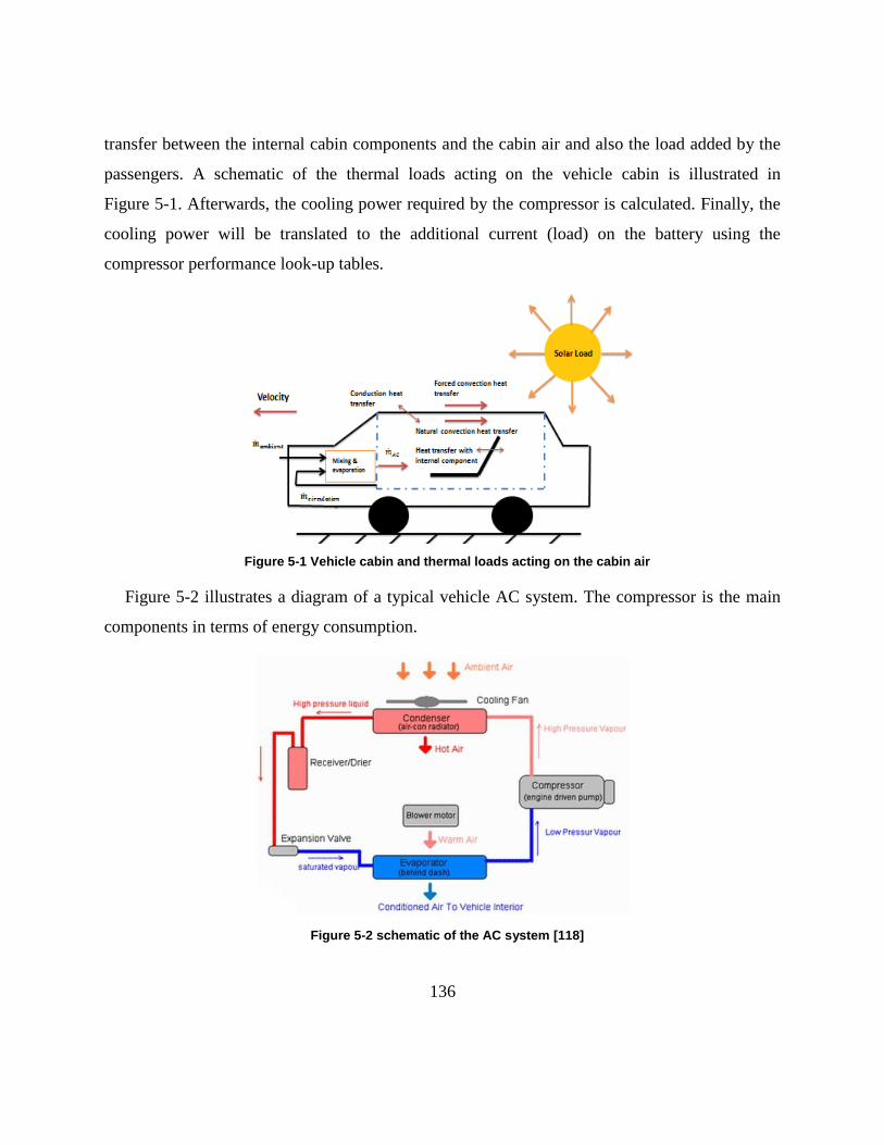
136
transfer between the internal cabin components and the cabin air and also the load added by the
passengers. A schematic of the thermal loads acting on the vehicle cabin is illustrated in
Figure 5-1. Afterwards, the cooling power required by the compressor is calculated. Finally, the
cooling power will be translated to the additional current (load) on the battery using the
compressor performance look-up tables.
Figure 5-1 Vehicle cabin and thermal loads acting on the cabin air
Figure 5-2 illustrates a diagram of a typical vehicle AC system. The compressor is the main
components in terms of energy consumption.
Figure 5-2 schematic of the AC system [118]
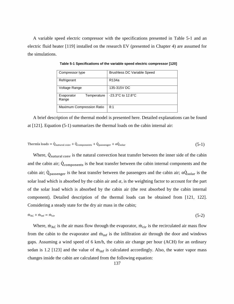
137
A variable speed electric compressor with the specifications presented in Table 5-1 and an
electric fluid heater [119] installed on the research EV (presented in Chapter 4) are assumed for
the simulations.
Table 5-1 Specifications of the variable speed electric compressor [120]
Compressor type Brushless DC Variable Speed
Refrigerant R134a
Voltage Range 135-315V DC
Evaporator Temperature Range
-23.3°C to 12.8°C
Maximum Compression Ratio 8:1
A brief description of the thermal model is presented here. Detailed explanations can be found
at [121]. Equation (5-1) summarizes the thermal loads on the cabin internal air:
Thermla loads = Qnatural conv + Qcomponents + Qpassenger + αQsolar (5-1)
Where, Qnatural conv is the natural convection heat transfer between the inner side of the cabin
and the cabin air; Qcomponents is the heat transfer between the cabin internal components and the
cabin air; Qpassenger is the heat transfer between the passengers and the cabin air; αQsolar is the
solar load which is absorbed by the cabin air and 𝛼, is the weighting factor to account for the part
of the solar load which is absorbed by the cabin air (the rest absorbed by the cabin internal
component). Detailed description of the thermal loads can be obtained from [121, 122].
Considering a steady state for the dry air mass in the cabin;
mAC + minf = mcir (5-2)
Where, mAC is the air mass flow through the evaporator, mcir is the recirculated air mass flow
from the cabin to the evaporator and minf is the infiltration air through the door and windows
gaps. Assuming a wind speed of 6 km/h, the cabin air change per hour (ACH) for an ordinary
sedan is 1.2 [123] and the value of minf is calculated accordingly. Also, the water vapor mass
changes inside the cabin are calculated from the following equation:
138
dWair
dt= (mairW) AC + (mairW) inf − (mairW) cir + mvap, passenger (5-3)
Where, W: absolute humidity, (kg water/ kg dry air). mvap, passenger: Vapor added from the
passengers exhale. According to the Equation (5-3), cabin vapor mass changes as a result of the
humidity addition by the air flowing through the AC blower, infiltration air flow, passengers
exhale and the vapor leaving the cabin through the recirculated air (from the cabin to the AC
cycle). The instantaneous cabin temperature is estimated based on the cabin air enthalpy, which
is calculated from the energy balance:
dHairdt
= thermal loads + (��H) AC + (��H) inf − (��H) cir
mair (5-4)
Where: Hair: Enthalpy of moist air. (��H) AC: Enthalpy flow through the evaporator to the
cabin
(��H) inf: Enthalpy flow from the ambient to the cabin through the unsealed doors & windows
(��H) cir: Enthalpy flow from the cabin to the AC cycle through recirculation
And finally the cabin air temperature is calculated based on the moist air enthalpy &
temperature relation:
𝑇𝑎𝑖𝑟 =𝐻𝑎𝑖𝑟 − 2501𝑊𝑎𝑖𝑟
1.006 + 1.805𝑊𝑎𝑖𝑟 (5-5)
Several parameters are required to be set before running the thermal model, such as the
dimensions and thermodynamic properties of the vehicle cabin (as well as the windows and
doors), weather conditions (solar load, humidity and temperature) and the AC running mode (i.e.
circulation coefficient). For the current analysis, those parameters that are not easily measurable
from the vehicle are borrowed from the literature for a regular sedan. The cabin dimensions and
thermodynamic properties used for the simulations are also presented in Table 5-2.

139
Table 5-2 Baseline vehicle dimensions and thermodynamic properties assumed for simulation
Cabin 3 (m3)
Wind shield 1.2x0.6x0.01 (m3)
Thermal conductivity: 1.4 (𝑊
𝑚𝐾)
Rear shield 1 x0.6x0.01 (m3)
Thermal conductivity: 1.4 (𝑊
𝑚𝐾)
Side wind 0.4x0.4x0.01 (m3)
Thermal conductivity: 1.4 (𝑊
𝑚𝐾)
Cabin internal component Equivalent area: 7 (m2)
Equivalent mass: 210 kg
Convective heat transfer coefficient: 100 (𝑊
𝑚2𝐾)
Specific heat capacity: 1.67 (𝑘𝐽
𝑘𝑔𝐾)
A fuzzy controller, shown in Figure 5-3 is also designed to control the AC (blower) air mass
flow rate to the cabin based on the instantaneous cabin temperature difference with the set point.
Due to the lack of field test data on the AC system components and to simplify the calculations,
it was assumed that the AC system is running under steady state condition and the air
temperature at the evaporator exit is 5 ℃ . However, once such data is available, a model of the
AC could be developed to account for the transient loads. For the heating scenarios, a
temperature of 22 ℃ is assumed at the inlet vent.
Figure 5-3 Fuzzy controller to determine the blower mass flow rate

140
5.3 Climate Scenarios
Three climate scenarios are assumed; each incorporating an ambient temperature condition
and initial battery pack temperature (Table 5-3). Scenario1 represents the average ambient
conditions in Toronto, Canada during June month with an average temperature of 25 (℃).
Scenario 2 represents a summer day in Arizona, the hottest area in the US. In scenario 3, a winter
day of Toronto in February month with an average ambient temperature of −8 (℃) is assumed.
Although ambient conditions have daily and annual variations, the present work neglects
temperature variation due to variable ambient conditions.
Table 5-3 Scenarios considered for simulating the temperature profile of vehicle cabin
Scenario 1-June, Toronto, 2-July, Arizona February, Toronto
Number of passengers 2 2 2
Solar irradiation 0.6 (
kW
m2 ) 1.1 (kW
m2 ) 0.2 (kW
m2 )
Ambient temperature 23 (℃) 35 (℃) −5 (℃)
Ambient Relative humidity 80 (%) 35 (%) 80(%)
Initial battery temperature 23 (℃)
35(ᵒC) −5 (℃) 25(ᵒC)
(Preconditioning) 5(℃)
(Preconditioning)
Initial cabin air temperature 42 (℃) 55 (℃) −5 (℃)
Initial cabin components temperature 47 (℃) 60 (℃) −5 (℃)
Initial cabin air humidity 60 (%) 30 (%) 60(%)
Drive cycle Test drive cycle
5.4 Results- Thermal model and A/C impacts
For the purpose of demonstration, the corresponding cabin temperature profile for scenario 1
and scenario 2 is plotted in Figure 5-4. The fuzzy controller determines the blower air flow rate
based on the difference observed between the cabin air temperature and the desire point.
Therefore, in the beginning of the simulation, the blower is set on maximum flow rate and the
cabin temperature experiences a sudden decrease in the first 100 second and converges to a

141
steady state afterwards. Figure 5-5 illustrates the profile of cabin air absolute humidity during
this simulation. As expected, decreasing the cabin air temperature results in a decrease in
humidity content of the air until a certain value is reached. Scenario 3 is used for degradation
studies in the next sections.
Figure 5-4. Cabin temperature profile- Test derive cycle
Figure 5-5. Profile of cabin absolute humidity under test drive cycle
Profile of the blower flow rate and the compressor current are plotted in Figure 5-6.Assuming
an ideal evaporator, the enthalpy change of air passing through the evaporator is equal to the
enthalpy change of the refrigerant and is assumed as the required cooling capacity (watt) from
the compressor. This cooling capacity is then translated into the required current by the
compressor. This is actually the extra load on the battery, which is shown in Figure 5-7.
Figure 5-6. Profile of air flow through the blower Figure 5-7. Profile of compressor current under test
0 100 200 300 400 500 60020
25
30
35
40
45
50
55
Time (sec)
Te
mpera
ture
(C
)
Scenario 1
Scenario 2
0 20 40 60 800.005
0.01
0.015
0.02
0.025
0.03
0.035
Time (sec)A
bso
lute
hu
mid
ity (
kg w
ate
r/kg a
ir)
Scenario 1
Scenario 2
0 100 200 300 400 500 6000.04
0.06
0.08
0.1
0.12
0.14
0.16
Time (sec)
Air
volu
me
(m
3/s
)
Scenario 2
Scenario 1
0 1000 2000 3000 40004
5
6
7
8
9
10
Time (sec)
Co
mpre
ssor
curr
ent
(A)
Scenario 1
Scenario 2

142
drive cycle
5.5 Vehicle Simulations
For the current study, vehicle models initially developed by UWAFT [96] in Autonomie are
used. The models include an E85 series extended range EV (EREV) as the baseline, and a pre-
transmission parallel architecture. Both models are conversions of Malibu 2013. These
architectures are illustrated in Figure 5-8 and Figure 5-9. Model inputs and the main powertrain
components (which are assumed similar in all configurations) are described in Table 5-4. Each of
these configurations creates a unique environment for the battery by allowing a different SOC
range and power demand on the battery. Unlike the NiMH batteries of the current CS hybrids,
which are operated over a small window (around 50% SOC), the batteries used in PHEVs
operate over a large SOC window. Starting from a certain high SOC (e.g. 90%), the vehicle
operates in a charge-depleting (CD) or an EV mode until a low SOC is reached. The battery
manufacturer sets the lower SOC operation limit for the battery based on life considerations. For
the PHEV cases SOC window of 90%-30% is assumed which is equivalent to a 40 mile AER.
Each configuration contains a battery model consisting of the equivalent circuit model and the
thermal ramp rate model presented earlier in Chapter 3. The battery pack is modeled by a linear
scale up of a cell neglecting the effect of cell to cell variation and unbalancing.
Figure 5-8 Graphical presentation of the EREV series architecture

143
Figure 5-9 Graphical presentation of the pre-transmission parallel architecture
Table 5-4 Component specifications and model inputs used in the Autonomie model of EREV [96]
Component Option
Engine GM LE9 Engine (E85) 2.4L E85 engine provided by GM.
Generator TM4 Motive (105kW)
ESS (Battery) A123 Battery Pack, (19.7kWh @ 346V)
Electric motor TM4 Motive (206kW)
Final drive Borg Warner eGearDrive
Chassis 2013 Malibu
Power convertor New Eagle DCDC Converter
Electrical accessory The average power draw from accessories was assumed to be 1500W Frontal area 2.06 (m
2)
Vehicle mass 2003.7 (kg)
Battery SOC window 90%-30%
Battery thermal management Natural air cooling
Drag coefficient, Cd 0.25
5.5.1 CD range and Fuel consumption
CD range and fuel consumption of each configuration were simulated considering the effect
of climate control loads and battery thermal preconditioning. Results show that the climate
control loads has a relatively large impact on CD range reduction; on the other hand, battery
thermal preconditioning plays a significant role on minimizing on range reduction due to the

144
climate control loads. The EV operation (CD mode) also represents the maximum battery usage
and is a good indicator of the maximum temperature rise that the battery would undergo during
vehicle operation.
Figure 5-10 and Figure 5-11 represent the CD range and battery temperature rise as a function
of minimum SOC in the baseline model (Series PHEV) (operating under UDDS drive cycle)
assuming no additional loads or preconditioning. The initial module temperature is set at five
levels (-5ᵒC to 35ᵒC). It is observed that the EV range and final module temperature have a semi-
linear correlation withΔSOC.
Figure 5-10 AER results for different minimum SOC Figure 5-11 Battery temperature at the end of AER
Figure 5-12 through Figure 5-15 presents the effect of climate control loads and
preconditioning on CD range and fuel economy. For fuel economy calculations, a utility factor
(UF) of 0.75 was assumed and the fuel consumption was calculated based on Equations (2-3)
through (2-5). Also, a 30% critical SOC was assumed.
In the series PHEV, fuel consumption is increased due to heating loads by 39% and the CD
range is reduced by 20%. Also, applying A/C reduces the fuel economy by 65% and the CD
range by 12%. Thermal preconditioning improves the situation by reducing the initial climate
control system load. In case of heating, thermal preconditioning improves the fuel economy by
6% and the CD range by 11%; where, in case of A/C, the corresponding values are 1.5 % and
2%.
15 20 25 30 35 4025
30
35
40
45
50
Critical SOC (%)
Ch
arg
e d
ep
leti
ng
ran
ge
(M
ile)
-5 ºC
0 ºC
12.5 ºC
23 ºC
35 ºC
15 20 25 30 35 400
5
10
15
20
25
30
35
40
45
Critical SOC (%)
Ch
arg
e d
ep
leti
ng
fin
al te
mp
era
ture
(ºC
)
-5 ºC
0 ºC
12.5 ºC
23 ºC
35 ºC

145
In case of parallel PHEV, using heat increases fuel consumption by 25% and decreases the
CD range by 19%. Using A/C increases fuel consumption by 40% and decreases the CD range
by 18%. Compared to no thermal preconditioning, thermal preconditioning with heat decreases
fuel consumption by 4% and increases the CD range by 9%. and thermal preconditioning with
A/C decreases fuel consumption by 3% and increases the CD range by 7%.
Figure 5-12 Series PHEV (EREV) CD range assumming 30% critical SOC
Figure 5-13 Series PHEV (EREV) fuel consumption assumming 30% critical SOC
Figure 5-14 Parallel PHEV CD range assumming 30% critical SOC
Figure 5-15 Parallel PHEV fuel consumption assumming 30% critical SOC
5.5.2 Degradation simulation
In this section, battery capacity fade is simulated under several operating conditions. The
common definition for battery end-of-life (EOL) is when battery remaining capacity has reached
-5 23 350
10
20
30
40
50
60
Temperature (ºC)
Ch
arg
e d
ep
leti
ng
ran
ge
(M
ile)
normal operation
preconditioned
climate control
climate control (preconditioned)
-5 23 350
0.5
1
1.5
2
2.5
3
3.5
4
4.5
Fu
el e
co
no
my (
litr
e/1
00k
m)
Temperature (ºC)
normal operation
precnditioning
climate control
climate control (preconditining)
-5 23 350
5
10
15
20
25
30
Temperature (ºC)
Ch
arg
e d
ep
leti
ng
ran
ge
(M
ile)
normal operation
preconditioned
climate control
climate control (preconditioned)
-5 23 350
0.5
1
1.5
2
2.5
3
3.5
4
Fu
el e
co
no
my (
litr
e/1
00k
m)
Temperature (ºC)
normal operation
preconditioned
climate control
climate control (preconditioned)
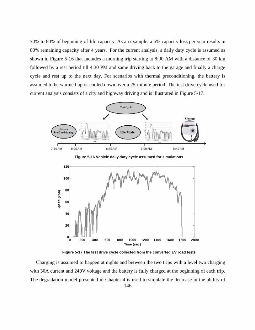
146
70% to 80% of beginning-of-life capacity. As an example, a 5% capacity loss per year results in
80% remaining capacity after 4 years. For the current analysis, a daily duty cycle is assumed as
shown in Figure 5-16 that includes a morning trip starting at 8:00 AM with a distance of 30 km
followed by a rest period till 4:30 PM and same driving back to the garage and finally a charge
cycle and rest up to the next day. For scenarios with thermal preconditioning, the battery is
assumed to be warmed up or cooled down over a 25-minute period. The test drive cycle used for
current analysis consists of a city and highway driving and is illustrated in Figure 5-17.
Figure 5-16 Vehicle daily duty cycle assumed for simulations
Figure 5-17 The test drive cycle collected from the converted EV road tests
Charging is assumed to happen at nights and between the two trips with a level two charging
with 30A current and 240V voltage and the battery is fully charged at the beginning of each trip.
The degradation model presented in Chapter 4 is used to simulate the decrease in the ability of
0 200 400 600 800 1000 1200 1400 1600 1800 20000
20
40
60
80
100
120
Time (sec)
Sp
eed
(k
ph
)

147
the battery to hold charge. Impact of climate control loads and preconditioning is incorporated in
the simulations. When the battery is preconditioned, it is exposed to a different temperature
range; therefore, the degradation rates will be different compared to a non-preconditioned case.
Also, in case of preconditioning, due to the temperature dependent available capacity, the battery
will experience a different depth of discharge (DOD) each day, which results in a different
degradation rate. Battery temperature rise results from multiple factors, namely battery thermal
mass, heat generation rate while driving, and rate of active cooling. A general comment on
preconditioning could be as follows: Battery packs with small battery thermal mass, high heat
generation rates, and limited or no active cooling while driving, likely to experience a large
temperature rise while driving and benefit most from pre-cooling will be those. In Figure 5-18 ,
the yearly percent of capacity loss for the series PHEV is presented at various ambient
temperatures, with and without climate control loads and preconditioning. Following observation
could be made:
Figure 5-18 Annual battery capacity loss rate in the series PHEV
The −5°C ambient case reduces fade by 53% relative to 23°C ambient. Thermal pre-
heating at -5°C ambient increases battery capacity loss by almost 5%. However at such
low temperatures, the small fade rates are relatively insignificant.
-5 23 350
2
4
6
8
10
12
Temperature (ºC)
Cap
ac
ity
lo
ss (
%)
normal operation
preconditioned
climate control
climate control (preconditioned)

148
The 35°C ambient case with no preconditioning increases capacity fade rates by 43%
(relative to 23°C ambient).
At hot ambient conditions (35°C), the most benefit from thermal pre-cooling is obtained;
which the capacity-fade rate is decreased by ~2%.
Heating and cooling load show a significant impact on the battery health. At −5°C,
heating load result in ~25% increased degradation and at 35°C, ~22% capacity loss rate is
accelerated.
Figure 5-19 shows battery degradation rates for the parallel PHEV. Generally, similar trends
are observed. At 35°C ambient, thermal preconditioning reduces capacity-loss rate by 3% and
the A/C loads adds a 17% on the capacity loss rate while heating results in a ~25% extra capacity
loss rate. The two vehicle platforms each derive slightly different benefits from pre-cooling,
partlyduetothesizeofeachvehicle’sbattery and partly due to the control strategies each layout
employs.
Figure 5-19 Battery capacity loss rate in the Parallel PHEV
5.6 Conclusions
In this chapter, impact of AC and heating loads on the Li-ion battery performance and
-5 23 350
2
4
6
8
10
12
Temperature (ºC)
Cap
ac
ity
lo
ss (
%)
normal operation
preconditioned
climate control
climate control (preconditioned)

149
degradation and vehicle electric range and fuel consumption was studied. A Thermal model of
the vehicle cabin was developed to predict the cabin temperature profile and required cooling/
heating load according to the set point. A model of Li-ion battery consisting of an equivalent
circuit and a regressive thermal model presented in Chapter 3 was coupled with the cabin
thermal model. The integrated model enables predicting the additional required power by the
A/C or heating system from the battery. It was observed that climate control loads significantly
increase fuel consumption and decrease CD range in PHEVs. To reduce these negative impacts,
off-board powered thermal preconditioning of the battery and vehicle cabin was shown to be an
efficient way.
150
Chapter 6
Conclusions and Recommendations
6.1 Conclusions and Contributions
In this thesis, Li-ion battery performance was studied through lab tests and in-situ vehicle
field measurements. Experiments included EIS tests and cycling tests at cell level and also in-situ
measurements from a converted electric vehicle (EV). Following conclusions could be made:
6.1.1 Thermal studies
Two commercially available battery cells were tested under a comprehensive set of charge
and discharge cycling tests and different ambient temperatures (-10ᵒC to 35ᵒC). The battery cells
were put in a jig to simulate battery pack condition in a vehicle. The energy efficiency and
columbic efficiency of the cells were determined for each testing condition. Results agreed with
the belief that the Li-ion cells have a better performance at higher temperatures. The temperature
distribution of the cells was also found to be approximately uniform across the cell thickness.
Heat generation of the cells was calculated assuming a natural convection mechanism for heat
rejection to the ambient air. A thermal ramp rate model was then developed for each cell and
operating mode using linear regression method. The model is able to predict the heat generation
rate and the cell temperature rise according to the cell SOC, load (current) profile and ambient
temperature. The model can be easily integrated with the battery model in Autonomie and is very
useful in powertrain design and drive cycle simulations, as it eliminates the need for a detailed
fundamental model with high computing cost.
151
6.1.2 EIS Tests and Modeling
A major objective in this research was to develop a battery performance model that could be
used for real-time applications, such as vehicle on-board BMS. For this purpose, the battery cells
were studied under a set of electrochemical impedance spectroscopy (EIS) tests. The cells’
response was measured over a frequency range of 10 µHz to 1 MHz at different temperatures
and SOCs. Based on the observed phenomenon from the frequency plots, an equivalent circuit
model was proposed and developed for both cells. The proposed model offers an improvement of
up to 6% in terms of average and maximum error in voltage predictions; which is still significant
for EV applications in terms of extending the allowable battery discharge window and the
vehicle range. In addition, the model capability in predicting HPPC test charge and discharge
resistances was verified. It was observed that this model could be used as an alternative to the
HPPC test within 20% error. The model shows the best performance at high temperatures which
could be due to experimental errors at lower temperatures as a result of cell self-heating. This
model is fast and easy to implement and is useful for hybrid powertrain design.
6.1.3 Field tests
Field tests were conducted with an electrified Ford Escape 2009 (EV-ACX2.5), belonging to
Burlington Hydro Company. The objectives of the field testing included three phases as follows.
Energy analysis
A study was conducted on the feasibility and advantages of replacing the conventional
(gasoline) fleet vehicles with the converted research EV. For this purpose, a data management
system was programmed and installed to collect and analyze operation data of baseline fleet
vehicles and EV-ACX2.5. Data of interest included charging and discharging events of EV-
ACX2.5 and drive cycles of the fleet vehicles. Each vehicle was instrumented with a data logger
that recorded and transmitted the data to a server. Having analyzed the data, detailed monthly
reports were generated for EV-ACX2.5 over a five-month period, which enabled tracking of the
vehicle’stotaldistancetravelled, energy consumption, efficiency, and charging times. The main

152
results are summarized as follows:
Over five months of operation (October 2011-February 2012), the EV-ACX2.5
travelled 792.6 kilometers and used 222.6 kWh of grid electricity during charging,
which yielded an average energy efficiency of 281 Wh/km.
In comparison with fleet vehicles, it was found that the EV-ACX2.5 is more than
50% cheaper to operate in terms of energy economy (km/$).
Powertrain Modeling and Fleet Analysis
The collected data were used to develop a powertrain model for the EV-ACX2.5 using PSAT
software. The model was then validated using real-life drive cycles collected during the vehicle
operation. Powertrain efficiency was also calculated through this model. It was observed that the
EV-ACX2.5 was operating with 77% energy efficiency on average, which confirms the
superiority of EVs to the conventional vehicles. The performance of the EV-ACX2.5 was also
evaluated as a fleet vehicle. This task was performed by running the EV-ACX2.5 PSAT model
undertheHEVs’drivecyclestofindouttheEV-ACX2.5 energy requirement for the same trips.
Results showed the EV-ACX2.5 can save almost 60% energy compared to the fleet vehicle.
Degradation studies
The collected data from the EV were also used to identify the degradation trends in the battery
pack. Power fade, capacity fade and charge efficiency fade were identified through the data as
three degradation metrics. A battery life model was also calibrated using the observed capacity
degradation over a four-month testing period. Validation of the model will be possible once more
data points are available. It was initially intended to develop an empirical life model of the
battery. Due to the limited data, the degradation study did not meet its targeted goal. However,
the analysis presented could be used as a pathway for future studies.

153
6.1.4 Vehicle lifetime studies
Chapter 5 described a battery life analysis under a different scenario, which included climate
control loads and battery preconditioning. Two PHEV powertrain architectures, including a
series and a parallel design, were developed in Autonomie. Assuming a similar battery pack for
both layouts, it was found that climate control system loads have a considerable impact on fuel
consumption (up to a 65% increase) and charge depletion (CD) range (up to a 20% decrease) in
PEVs. Off-board powered thermal preconditioning of a vehicle cabin and battery pack is an
effective way to reduce the negative impact of climate control system loads. It was observed that
thermal preconditioning can provide a moderate reduction in fuel consumption (up to 6%) and
partially restores CD range (up to 11%) which translates to several kilometers of CD range. Also,
in hot (35°C) ambient conditions, a pre-cooling of electric-drive vehicle batteries was observed
to reduce capacity fade by 3% and climate control loads accelerated the capacity fade by 22% to
25%. All in all, off-board powered thermal preconditioning benefits both the consumer (via CD
range extension) and vehicle manufacturers (via improved battery life and reduced warranty
services).
Overall, this thesis contribution was to address the performance of the Li-ion battery in
electrified vehicles and the direct and indirect impact of temperature on the battery performance
and degradation. Fast and accurate models of battery performance and heat generation were
developed for use in powertrain design and a degradation study through field tests was
attempted. The indirect impact of temperature, i.e. climate control loads and preconditioning
impacts, on the vehicle range and battery life, was modeled through coupling these models with
a thermal model of a vehicle cabin.
6.2 Recommendations
The presented study provides a framework for model based design of PHEVs focusing on Li-
ion battery. There are a number of potential extensions and recommendations that could be
considered for future research:
154
6.2.1 Thermal testing
In the current analysis, the convective heat transfer coefficient was assumed to be at its
natural convection value. However, the chamber fan turns on and off to control the chamber,
which results in a varying convective heat transfer coefficient during cycling. Therefore, it would
be beneficial to use a calorimeter to measure the cell heat transfer coefficient with a higher
accuracy at different states (natural and forced convection).
The regression models are limited to the parameters’ range in the tests. In the thermal
characterization tests, C-rates were chosen to vary from 0.5 to 4.5 in discharge. In a real case of
battery operation on a PHEV, C-rate could vary from values very close to zero up to 5.
Therefore, it would be desirable to add more testing points to further widen the range as well as
increase the homogeneity of the test domain.
The analysis and validation were based on cell level. However, single cell characteristics may
not be linearly scaled to a module or pack level system. For example, the resistance observed
from a single cell would include contact resistance where the cell tabs are bolted to the test
cables. In a production battery pack, the tabs would be welded to a bus bar, thereby changing the
resistance characteristics. Evaluating the internal resistance of a full battery pack would improve
the fidelity of the model and yield more accurate vehicle simulation results. Therefore, pack level
testing should be planned and carried out in future research.
It would be also desirable to repeat the thermal tests with different boundary conditions; i.e. a
water cooling case versus forced air cooling and no cooling to enable the analysis of different
battery thermal management strategies.
6.2.2 EIS testing
In the presented analysis, the regression models developed for each of the equivalent circuit
model parameters are based on a limited number of test points, which would affect the regression
capability in predicting the points that are far from the test points. Considering that the Li-ion

155
battery has a highly nonlinear dynamic, it is recommended that the EIS tests be repeated at more
SOCs (especially between 30%-60%). In addition, as the battery ages, its electrochemical
impedance spectra undergoes a shifts to the right and expansion resulting in the circuit
parameters (resistance and capacitor values) to change [30]. Therefore, it would be necessary to
consider the aging in the model development to reflect a more realistic perspective of the battery
behavior in vehicle simulations.
The proposed model was based on the data of three positive temperatures (12.5ºC, 23.75ºC
and 35ºC). Due to the limited availability of the EIS machine at the time of this research and
uncertainty in the collected data, the low temperatures (1.25ºC and -10ºC) were ignored in the
model development. It would be reasonable to repeat the tests at these temperatures to
incorporate the low temperature battery response in the model development.
6.2.3 Field testing
While field testing provides a valuable opportunity to analyze the battery pack behavior under
real-life operation, it is highly associated with uncertainty. There are several uncontrolled
parameters while the vehicle is in operation or even in idle mode. In such situations, relying on a
single vehicle for developing a battery life model adds more limitations to the analysis.
Therefore, if circumstances permit, it is recommended to get a number of electrified vehicles
instrumented and data logged. Additionally, as the battery aging happens over a 5-10 year period
(battery manufacturer set point) and considering the nonlinear nature of battery degradation, data
logging should be conducted over a wide time span so that the battery experiences different
stages of aging. This way, model development and calibration tasks could be carried out with a
higher accuracy. To improve the fleet study, the following studies are suggested:
Develop a validated model of a baseline fleet vehicle in PSAT (once the powertrain
data through CAN Bus is accessible).
Comparison between the EV-ACX2.5 and the fleet vehicle, in terms of emissions and
energy consumption over standard and real-life drive cycles.

156
Suggested improvements to the EV PSAT model are:
For vehicle level simulations, temperature-dependent models for other major
powertrain components, such as electric motors, should be created to more accurately
model how total vehicle efficiency changes with temperature. Accurate representation
of the entire vehicle is required to accurately predict vehicle range, performance, and
overall energy consumption. As the vehicle model matures, it will also serve as a
platform for developing vehicle control systems, torque splitting strategies and other
optimization algorithms.
6.2.4 Battery lifetime modeling
In the presented study of auxiliary loads’ impact on the battery, lack of experimental data
made the author make some simplifying assumptions. Among these assumptions, the evaporator
exit temperature was assumed a constant conveying steady state operation. However, to better
quantify the loads imposed by the climate control system, a model of A/C system and heating
system would be necessary, provided that technical data is available. In addition, validation of
the climate control model requires a wind tunnel and an instrumented vehicle would be necessary
for measuring the cabin temperature profile under different ambient conditions.
It is suggested that the battery degradation be analyzed under different control strategies.
There is always a trade-off between the fuel replacement and battery degradation; i.e. high
battery discharge results in better fuel economy but accelerates the battery capacity loss. There is
different control strategies proposed for PHEVs, so far. Among these strategies, thermostat
control, load-following control and cost based on control are three popular methods, which each
provide a unique environment and load profile for the battery [39].

References
[1] M. Ehsani, Y. Gao, A. Emadi, Modern Electric, Hybrid Electric, and Fuel Cell Vehicles: Fundamentals,
Theory, and Design, second ed., CRC Press, 2009.
[2] D. Howell, Annual Progress Report for Energy Storage R&D, Vehicle Technologies Program, Energy
Efficiency and Renewable Energy, Washington, DC, 2011.
[3] S. Dhameja, Electric Vehicle Battery Systems, Butterworth-Heinemann, 2002.
[4] G. Duleep, H.V. Essen, B. Kampman, M. Grünig, Impacts of Electric Vehicles - Deliverable 2 Assessment of
Electric Vehicle and Battery Technology, CE Delft, 2011.
[5] Pollution Probe, Driving Electric: Understanding Electric Vehicle Technology and Environmental Benefits,
2015.
[6] W. Liu, Introduction to Hybrid Vehicle System Modeling and Control, John Wiley & Sons Inc., 2013.
[7] A.W. Stienecker, An Ultracacitor-Battery Energy Storage System for Hybrid Electric Vehicles, Electrical
engineering, University of Toledo, 2005.
[8] D. Stotingco, A Simulation-Based Assessment of Plug-in Hybrid Electric Vehicle Architectures, Mechanical
engineering, Massachusetts Institute of Technology, 2010, pp. 85.
[9] F.R. Kalhammer, B.M. Kopf, D.H. Swan, V.P. Roan, M.P. Walsh, Status and Prospects for Zero Emissions
Vehicle Technology, Report of the ARB Independent Expert Panel, 2007.
[10] D. Kodjak, Consumer Acceptance of Electric Vehicles in the US, Mobile Source Technical Review
Subcommittee International Council of Clean Transportation (ICCT), EPA, Washington DC, 2012.
[11] Accenture, Final Report:Plug-in Electric Vehicles Changing Perceptions, Hedging Bets, 2011.
[12] B. Pattipati, C. Sankavaram, System Identification and Estimation Framework for Pivotal Automotive Battery
Management System Characteristics, IEEE Transaction on Vehicular Technology, 4 (2011) 869-884.
[13] Y. Xing, Ma, E., Tsui, K. L. , Pecht, M., Battery Management Systems in Electric and Hybrid Vehicles,
Energies, 4 (2011) 1840-1857.
[14] M. Doyle, T.F. Fuller, J. Newman, Modeling of Galvanostatic Charge and Discharge of the
Lithium/Polymer/Insertion Cell, J. Electrochemical Society, 140 (1993) 1526–1533.
[15] X. Hu, S. Li, H. Peng, A Comparative Study of Equivalent Circuit Models for Li-ion Batteries, J. Power
Sources, 198 (2012) 359-367.
[16] B. Martin, A Dynamic Battery Model Considering the Effects of the Temperature and Capacity Fading,
Elektrotechnika, (2012).
158
[17] H. Zhang, Chow, M-Y. , Comprehensive Dynamic Battery Modeling for PHEV Applications, Power and
Energy Society General Meeting, 2010, pp. 1-6.
[18] J. Zhang, C. Song, H. Sharif, M. Alahmad, An Enhanced Circuit-Based Model for Single-Cell Battery,
Applied Power Electronics Conference and Exposition (APEC), 25th Annual IEEEPalm Springs, CA, 2010, pp.
672 - 675.
[19] S.S. Zhang, Xu, K., Jow, T.R., Electrochemical Impedance Study on the Low Temperature of Li-ion Batteries,
Electrochim. Acta, 49, no. 7 (2004) 1057-1061.
[20] F. Baronti, G. Fantechi, E. Leonardi, R. Roncella, Enhanced Model for Lithium-Polymer Cells Including
Temperature Effects, 36th Annual Conference on IEEE Industrial Electronics Society, IEEE, Glendale, AZ,
2010, pp. 2329 - 2333.
[21] Y. Hu, S. Yurkovich, Y. Guezennec, B.J. Yurkovich, Electro-Thermal Battery Model Identification for
Automotive Applications, J. Power Sources, 196 (2011) 449-457.
[22] W. Waag, Kabitz, S.,Sauer, D. U., Experimental Investigation of the Lithium-ion Battery Impedance
Characteristic at Various Conditions and Aging States and its Influence on the Application, Applied Energy,
102 (2013) 885-897.
[23] C.H. Chen, J. Liu, K. Amine, Symmetric Cell Approach and Impedance Spectroscopy of High Power
Lithium-ion Batteries,, J. Power Sources, 96 (2001) 321-328.
[24] R.E. Williford, Viswanathan, V. V., Zhang, J., Effects of Entropy Changes in Anodes and Cathodes on the
Thermal Behavior of Lithium-ion Batteries, Journal of Power Sources, 189 (2009).
[25] k. Parsons, Design and Simulation of Passive Thermal Management System for Lithium-ion Battery Packs on
an Unmanned Ground Vehicle, Mechanical Engineering, California Polytechnic State University, 2012.
[26] S. Al Hallaj, H. Maleki, J.S. Hong, J.R. Selman, Thermal Modeling and Design Considerations of lithium-ion
Batteries, J. Power Sources, 83 (1999) 1–8.
[27] W.B. Gu, C.Y. Wang, Thermal and Electrochemical Coupled Modeling of a Lithium-Ion Cell, J.
Electrochemical Society, 99 (2000) 748 - 762.
[28] P. Taheri, M. Bahrami, Temperature Rise in Prismatic Polymer Lithium-Ion Batteries:An Analytic Approach,
SAE International, , SAE, 2012.
[29] P. Rong, Pedram, M., An Analytical Model for Predicting the Remaining Battery Capacity of Lithium-ion
Batteries, Very Large Scale Integration (VLSI) Systems, IEEE Transactions, 14 (2006) 441-451.
[30] Y. Zhanga, C.Y. Wanga, X. Tang, Cycling Degradation of an Automotive LiFePO4 Lithium-ion Battery,
Journal of Power Sources, 196 (2011) 1513–1520.

159
[31] E. Prada, D. Di Domenicoa, Y. Creffa, J. Bernarda, V. Sauvant-Moynota, F. Huetb, A Simplified
Electrochemical and Thermal Aging Model of LiFePO4-Graphite Li-ion Batteries: Power and Capacity Fade
Simulations, J. Electrochemical Society, 160 (2013) 616-628.
[32] M. Dubarry, V. Svoboda, R. Hwu, B.Y. Liaw, A Roadmap to Understand Battery Performance in Electric and
Hybrid Vehicle Operation, J. Power Sources, (2007) 366–372.
[33] V. Klass, M. Behm, G. Lindbergh, Evaluating Real-Life Performance of Lithium-Ion Battery Packs in Electric
Vehicles Electrochemical Society, 41 (2012).
[34] A. Barré, F. Suard, M. Gérard, M. Montaru, D. Riu, Statistical Snalysis for Understanding and Predicting
Battery Degradations in Real-life Electric Vehicle Use, Journal of Power Sources, 245 (2014).
[35] H. Khayyam, S. Nahavandi, E. Hu, A. Kouzani, A. Chonka, J. Abawajyd, V. Maranoe, S. Davisf, Intelligent
Energy Management Control of Vehicle Air Conditioning via Look-ahead System, J. Applied Thermal
Engineering, 31 (2011) 3147-3160.
[36] J. Larminie, Lowry, J., Electric Vehicle Technology Explained, John Wiley and John Lowry2003.
[37] NREL, NREL Reveals Links Among Climate Control, Battery Life, and Electric Vehicle Range, 2012.
[38] E. Samadani, Gimenez, L., Scott, W., Farhad, S., Fowler, M., Fraser, R. A., Thermal Behavior of Two
Commercial Li-Ion Batteries for Plug-in Hybrid Electric Vehicles 2014, SAE World Congress, Detroit, MI,
2014.
[39] E. Samadani, S. Farhad, W. Scottc, M. Mastalia, L.E. Gimenezc, M. Fowlerc, R.A. Frasera, Empirical
Modeling of Lithium-ion Batteries Based on Electrochemical Impedance Spectroscopy Tests, Electrochimica
Acta, 160 (2015) 169–177.
[40] E. Samadani, S. Panchal, M. Mastali, R.A. Fraser, Battery Life Cycle Management for Plug-in Hybrid Electric
Vehicle (PHEVs) and Electric Vehicles (EVs), Transport Canada Final Report, Transportation Development
Centre Of Transport Canada, University of Waterloo, 2012, pp. 88.
[41] S.S. Zhang, A Review on the Separators of Liquid Electrolyte Li-ion Batteries, Journal of Power Sources, 164
(2007) 351-364.
[42] M. Dubarry, V. Svoboda, R. Hwu, B.Y. Liaw, Capacity Loss in Rechargeable Lithium Cells during Cycle Life
Testing: The Importance of Determining State of Charge, J. Power Sources, 174 (2007) 1121-1125.
[43] I.N. Laboratory, Battery Test Manual for Plug in Hybrid Electric Vehicles, September 2010.
[44] M.D.a.B.Y. Liaw, Identify Capacity Fading Mechanisms in a Commercial LiFePO4 Cell, J. Power Sources,
194 no.1 (2009) 541‐549.
[45] E. Samadani, Lo, J., Fowler,M., Fraser, R. A., Gimenez,L., Impact of Temperature on the A123 Li-Ion Battery
Performance and Hybrid Electric Vehicle Range, SAE Detroit, 2013.

160
[46] S. Pillar, Perrin, M., Jossen, A. , Methods for State-of-Charge Determination and their Applications, Journal
of Power Sources, 96 (2001) 113-120.
[47] W. Tahil, How Much Lithium Does a Li-ion EV Battery Really Need?, Meridian International Research,
(March 2010).
[48] V. Viswanathan, D. Choi, D. Wang, W. Xu, S. Towne, E. Williford, G. Zhang, J. Liu, Z. Yang, Effect of
Entropy Change of Lithium Intercalation in Cathodes and Anodes on Li-ion Battery Thermal Management, J.
Power Sources, 195, no. 11 (2010) 3720‐3729.
[49] H.G. Schweiger, O. Obeidi, O. Komesker, A. Raschke, M. Schiemann, C. Zehner, M. Gehnen, M. Keller, P.
Birke, Comparison of Several Methods for Determining the Internal Resistance of Lithium Ion Cells, J. Sensors,
10 (2010) 5604-5625.
[50] D. Linden, T.B. Reddy, Handbook of Batteries, 3rd
ed., McGraw-Hill2001.
[51] G.A. Nazri, G. Pistaoie, Lithium Batteries, Science and Technology, Kluwer Academic Publishers2004.
[52]M.Shnayerson,TheCarThatCould.TheInsideStoryofGM’sRevolutionaryElectric
Vehicle, 1996.
[53] V. Srinivasan, J. Newman, A Model-based Comparison of Various Li-ion Chemistries, (2006).
[54] W. Mehrens, P. Axmann, M. Wachtler, Electrochemical Energy Storage Systems for Car Applications, Pres.
HySA Systems Business Seminar, (November 2009).
[55] R. Lache, P. Nolan, D. Galves, G. Toulemonde, J. Gehrke, K. Sanger, V. Ha, S. Rao, J. Crane, Electric Cars:
Plugged In. Batteries Must Be Included, Deutsche Bank AG, 2008.
[56] Battery University, Types of Lithium-ion, 2015.
[57] P. Arora, Z. Zhang, Battery Separators, J. Chem. Rev, 104 (2004) 4419-4462.
[58] M. Brain, How Lithium-ion Batteries Work, Howstuffworks
[59] O. Erdinc, B. Vural, M. Uzunoglu, A dynamic Lithium-ion Battery Model Considering the Effects of
Temperature and Capacity Fading, Clean Electrical Power, 2009 International Conference, IEEE, 2009, pp.
383–386.
[60] L. Lam, Bauer, P., Kelder, E., A Practical Circuit-Based Model for Li-ion Battery Cells in Electric Vehicle
Applications, in Telecommunications Energy Conference (INTELEC), IEEE 33rd International, 2011, pp. 1–9.
[61] A. Ostadi, M. Kazerani, S.-K. Chen, Optimal Sizing of the Energy Storage System (ESS) in a Battery-Electric
Vehicle, Transportation Electrication Conference and Expo (ITEC), IEEE, IEEE, 2013, pp. 1–6.
[62] J. Newman, W. Tiedemann, Porous-Electrode Theory with Battery Application, AIChE, 21 (1975) 25-41.

161
[63] T.F. Fuller, M. Doyle, J. Newman, Simulation and Optimization of the Dual Lithium Ion Insertation Cell, J.
Electrochemical Society, 141 (1994) 1-10.
[64] C.Y. Wang, W.B. Gu, B.Y. Liaw, Micro-Macroscopic Coupld Modeling of Batteries and Fuel Cells: Part II:
Applications to Ni-Cd and Ni-MH Cells, J. Electrochemical Society, 145 (1998) 3418 - 3427.
[65] H. He, R. Xiong, J. Fan, Evaluation of Lithium-Ion Battery Equivalent Circuit Models for State of Charge
Estimation by an Experimental Approach, J. Energies, 4 (2011) 582-598.
[66] C. Lin, B. Qiu, Q. Chen, Comparison of Current Input Equivalent Circuit Models of Electrical Vehicle
Battery, Chinese J. Mech. Eng., 41 (2005) 76-81.
[67] B.Y. Liaw, M. Dubarry, From Driving Cycle Analysis to Understanding Battery Performance in Real-life
Electric Hybrid Vehicle Operation, J. Power Sources, (2007) 76–88.
[68] I. Buchmann, How to Store Batteries, Battery University, 2015.
[69] Q. Zhang, White, R.E., Capacity Fade Analysis of a Lithium-ion Cell, J. Power Sources, 179, no. 2 (2008)
793-798.
[70] R. Spotnitz, Simulation of Capacity Fade in Lithium-ion Batteries, J. Power Sources, 113, no. 1 (2003) 72-80
[71] Electropaedia, Cell Chemistries-How Batteries Work, 2015.
[72] K. Edström, T. Gustafsson, J.O. Thomas, The Cathode–Electrolyte Interface in the Li-ion Battery, J.
Electrochim. Acta, 50 (2004) 397–403
[73] J. Vetter, P. Novák, M.R. Wagner, C. Veit, K.-C. Möller, J.O. Besenhard, M. Winter, M. Wohlfahrt-Mehrens,
C. Vogler, A. Hammouche, Ageing Mechanisms in Lithium-ion Batteries, J. Power Sources, 147, (2005) 269-
281.
[74] S.B. Peterson, J. Apt, J.F. Whitacre, Lithium-ion Battery Cell Degradation Resulting from Realistic Vehicle
and Vehicle-to-Grid Utilization, J. Power Sources, 195, no. 8 (2010) 2385-2392.
[75] C. Rosenkranz, Plug In Hybrid Batteries, Pres EVS20, (November 2003) 14.
[76] A. Pesaran, M. Keyser, G. Kim, S. Santhanagopalan, K. Smith, Tools for Designing Thermal Management of
Batteries in Electric Drive Vehicles, Large Lithium Ion Battery Technology & Application Symposia
Advanced Automotive Battery ConferencePasadena, CA, 2013.
[77] T.D. Tran, J.H. Feikert, R.W. Pekala, Rate Effect on Lithium-ion Graphite Electrode
performance, J. Appl. Electrochem, 26, no. 11 (1996) 1161-1167.
[78] K. Anime, J. Liu, I. Belharouak, High-temperature Storage and Cycling of CLiFePO4/ graphite Li-ion Cells, J.
Electrochem. Com, 7 (2005) 669-673.
162
[79] M. Broussely, Aging Mechanisms and Calendar Life Predictions in Lithium-ion Batteries, J. Advances in Li-
ion batteries, (2002) 293-432.
[80] P. Arora, R.E. White, M. Doyle, Capacity Fade Mechanisms and Side Reactions in Lithium-ion Batteries, J.
Electrochem. Soc., 145 (1998) 3647‐3666.
[81] H. Maleki, J.N. Howard, Effects of Overdischarge on Performance and Thermal Stability of a Li-ion Cell, J.
Power Sources, 160 (2006) 1395-1402.
[82] C. Kishiyama, M. Nagata, T. Piao, J. Dodd, P. Lam, H. Tsukamoto, Improvement of Deep Discharge
Capability for Lithium Ion Batteries, 205th Electrochemical Society Fall Meeting, 2003, pp. 252-259.
[83] J. Gonder, A. Simpson, Measuring and Reporting Fuel Economy of Plug-In Hybrid Electric Vehicles 22nd
International Battery, Hybrid and Fuel Cell Electric Vehicle Symposium and Exhibition, NREL, Yokohama,
Japan, 2006.
[84] J. Gonder, A. Brooker, J. Smart, Deriving In-Use PHEV Fuel Economy Predictions from Standardized Test
Cycle Results, 5th IEEE Vehicle Power and Propulsion Conf., IEEE, Dearborn, Michigan, 2009.
[85] L. Drew, S. Jim, M. Raffaello, O. Francisco, B. Colin, A High Performance Aircraft Wind Tunnel Test Using
Response Surface Methodologies, 2005 U.S. Air Force T&E Days, American Institute of Aeronautics and
Astronautics2005.
[86] MathWorks Documentation Center, Skewness, 2015.
[87] Wolfram Mathworld, Skewness, 2015.
[88] C.K. Dyer, P.T. Moseley, Z. Ogumi, D.A. Rand, B. Scrosati, Encyclopedia of Electrochemical Power Sources,
Elsevier Science2013.
[89] C. Vincent, B. Scrosati, Modern Batteries: An Introduction to Electrochemical Power Sources, 2 ed.,
Butterworth-Heinemann1997.
[90] N.R. Draper, H. Smith, Applied Regression Analysis, Wiley-Interscience1998.
[91] M. Chen, G.A. Rincón-Mora, Accurate Electrical Battery Model Capable of Predicting Runtime and IV
Performance, Energy Conversion IEEE Trans., 21 (2006) 504-511.
[92] C. Mi, B. Li, D. Buck, N. Ota, Advanced Electro-Thermal Modeling of Lithiumion Battery System for Hybrid
Electric Vehicle Applications, Vehicle Power and Propulsion Conference (VPPC), IEEE, IEEE, Arlington, TX,
2007, pp. 107–111.
[93] J. Shen, S. Dusmez, A. Khaligh, An Advanced Electro-Thermal Cycle-Lifetime Estimation Model for
LiFePO4 Batteries, Transportation Electrification Conference and Expo (ITEC), IEEE, 2013, pp. 1–6.
[94] A. Pesaran, Battery Thermal Models for Hybrid Vehicle Simulations, J. Power Sources, 110 (2002) 377–382.

163
[95] A. Pesaran, S. Santhanagopalan, G. Kim, Addressing the Impact of Temperature Extremes on Large Format
Li-Ion Batteries for Vehicle Applications, National Renewable Energy Laboratory, 2013.
[96] University of Waterloo alternative fuel Team (UWAFT), Design Report 5, University of Waterloo
Waterloo, 2012.
[97] S. Buller, M. Thele, E. Karden, R.W. Doncker Impedance-Based Non-Linear Dynamic Battery Modeling for
Automotive Applications, J. Power Sources, 113 (2003) 422-430.
[98] N. Lotfi, P. Fajri, S. Novosad, J. Savage, Development of an Experimental Testbed for Research in Lithium-
Ion Battery Management Systems, J. Energies, 6 (2013) 5231-5258.
[99] M.E. Orazem, B. Tribollet, Electrochemical Impedance Spectroscopy, Angew. Chem. Int. Ed.2009.
[100] D.V. Do, C. Forgez, K. El Kadri Benkara, G. Friedrich, Impedance Observer for a Li-Ion Battery Using
Kalman Filter, Vehicle Tech. IEEE Trans., 58 (2009) 3930-3937.
[101] Zmantechnologies, Zman User's Manual, WonATech Co. LTD, Seoul, Korea, 2014.
[102] I.N. Laboratory, Battery Test Manual for Plug-In Hybrid Electric Vehicles Rev. 1, U.S. Dept. of Energy
Vehicle Technologies Program, 2010.
[103] S. Yuan, H. Wu, C. Yin, State of Charge Estimation Using the Extended Kalman Filter for Battery
Management Systems Based on the ARX Battery Model, J. Energies, 6 (2013) 444-470.
[104] E. Samadani, J. Lo, M. Fowler, R. Fraser, L. Gimenez, Impact of Temperature on the A123 Li-Ion Battery
Performance and Hybrid Electric Vehicle Range, SAE World Congress,, SAE, Detroit, MI, 2013.
[105] Y. Zheng, M. Ouyang, L. Lu, J. Li, X. Han, L. Xu, H. Ma, T.A. Dollmeyer, V. Freyermuth, Cell State-of-
Charge Inconsistency Estimation for LiFePO4 Battery Pack in Hybrid Electric Vehicles Using Mean-Difference
Model, J. Applied Energy, 111 (2013) 571-580.
[106] K.S. Hariharan, V.S. Kumar, A Nonlinear Equivalent Circuit Model for Lithium-ion Cells, J. Power Sources,
222 (2013) 210-217.
[107] M. Greenleaf, H. Li, J.P. Zheng, Modeling of LixFePO4 Cathode Li-Ion Batteries Using Linear Electrical
Circuit Model, IEEE Trans., 4 (2013) 1065-1070.
[108] H. Abu-Rub, M. Malinowski, K. Al-Haddad, Power Electronics for Renewable Energy Systems,
Transportation and Industrial Applications, Wiley2014.
[109] Burlington Hydro, GridSmartCity® – Providing a Forum for Dialogue and Discovery.
[110] M. Giannikouris, Battery Lifecycle Management for PHEVs: Transport Canada Final Report, University of
Waterloo, 2010, pp. 44.

164
[111] S.P. E. Samadani, M. Mastali, and R. A. Fraser, Battery Life Cycle Management for Plug-in Hybrid Electric
Vehicle (PHEVs) and Electric Vehicles (EVs), University of Waterloo, 2012.
[112] Argonne National Laboratory, PSAT (Powertrain System Analysis Toolkit), Argonne, Transportation
Technology R&D Center.
[113] D. Montgomery, Determining the Specific Heat Capacity of a Battery Pack; Illustrative Example and
Description of Method.
[114] G. Ning, R.E. White, B.N. Popov, A Generalized Cycle Life Model of Rechargeable Li-ion Batteries, J.
Electrochimica Acta, 51 (2006) 2012-2022.
[115] M.B. Stevens, Hybrid Fuel Cell Vehicle Powertrain Development Considering Power Source Degradation,
University of Waterloo, 2008.
[116] Y. Li, Scenario-Based Analysis on the Impacts of Plug-In Hybrid Electric Vehicles' (PHEV) Penetration into
the Transportation Sector, IEEE International Symposium on Technology and SocietyLas Vegas, NV, 2007,
pp. 1-6.
[117] R.A. Barnitt, A.D. Brooker, L. Ramroth, J. Rugh, K.A. Smith, Analysis of Off-Board Powered Thermal
Preconditioning in Electric Drive Vehicles, 25th World Battery, Hybrid and Fuel Cell Electric Vehicle
Symposium & ExhibitionShenzhen, China, 2010.
[118]BlueDevilProduct,HowDoIRepairMyCar’sAC?
[119] Metric Mind Corporation (MMC), EV Fluid Heaters, Metric Mind Corporation.
[120] Masterflux, Compressor Data Sheet, Master Flux Products.
[121] C.D. Haung, A Dyanamic Computer Simulation Model for Automobile Passenger Compatment Climate
Control and Evaluation, Mechanical Engineering, Michigan Technological University, 1998.
[122] S. Sanaye, M. Dehghandokht, A. Fartaj, Temperature control of a Cabin in an Automobile using thermal
Modeling and Fuzzy Controller, J. Applied Energy, 97 (2012) 860-868.
[123] L. Knibbs, R. de Dear, S. Atkinson, Field Study of Air Change and Flow Rate in Six Automobiles, J. Indoor
Air,, 19 (2009) 303-313.

165
Appendix-A
Statistical Analysis of Cell Temperature Distribution
Investigating the coefficients of skew for each of the examined readings reveals different distribution
behavior for each cell (A 1and A 2).
A 1: Skew coefficient for experiments performed with Cell 1. The color code indicates SOC (blue=0%, red=50%, black=100%) and marker code indicates discharge and charge c-rate (charge: x=0.25, *=1.25, o=2.25; discharge:
diamond=0.5, square=2.5, +=4.5)
A 2: Skew coefficient for experiments performed with Cell 2. The color code indicates SOC (blue=0%, red=50%, black=100%) and marker code indicates discharge and charge c-rate (charge: x=0.25, *=1.25, o=2.25; discharge:
diamond=0.5, square=2.5, +=4.5
For cell 1, over half of the sampled points there is evidence of a skewed distribution as the coefficient
values fall outside the 90% confidence interval bounds with n=12. These confidence bounds are ±1.049
(in both batteries) and were obtained by fitting and extrapolating a table of 90% confidence bounds for

166
the skewness coefficient [20]. In contrast, all of the coefficients for cell 2 fall between the bounds
suggesting the presence of a centered distribution.
Given that a large number of beginning-, middle-, and end-of-step skew coefficients fall outside the
confidence bounds, and that these skew coefficients are neither consistently positive nor negative, it can
be assumed that the observed skew in the temperature distributions is caused by factors other than the
heat generation of the cell. Since cell 1 was on the bottom shelf of the chamber, it was a further distance
from the chamber circulation fan. It is therefore possible that the location increases the likelihood of non-
uniform temperature variations. This hypothesis is endorsed by the low difference between the mean and
the median for cell 1.
The average difference between the mean and median of the temperature readings (A 3 and A 4) is
−0.014K/−0.0075Kforthechargeanddischargestepsofcell1and0.089K/0.030Kforthesamestepsof
cell 2, respectively. The difference between mean and median rarely exceeded ±0.15K at the end or
middle of step for both cells. This difference was consistently of greater magnitude for cell 2, centered at
0.05K, but this is still well within the margin of error. Further, the analysis of skew coefficients suggests
thereisnoskeweddistributionatanypointforthiscell.Thestandarddeviation(σ)ofthetemperatures
shows no consistent effect of chamber temperature or charge/discharge C-rate on the temperature spread.
Thissuggestsevenlydistributedheatingofthecell.Theaverageσwascalculatedtobe0.227K/0.368K
for charge/discharge of cell 1 and 0.221K/0.302K for the charge/discharge of cell 2. While this
temperature spread is higher than the error in the thermocouples, it is not greater than the chamber
temperaturecontrolrange(±0.5K).Further,thelargervaluesofσ(above0.5K)almostallcorrespondto
the initial SOC of the charge or discharge step, with the value decreasing as the step is carried out (with
two minor exceptions). This suggests the influence of environmental factors on the temperature
distribution causes greater spread than any internal differences in the heat generation rate.
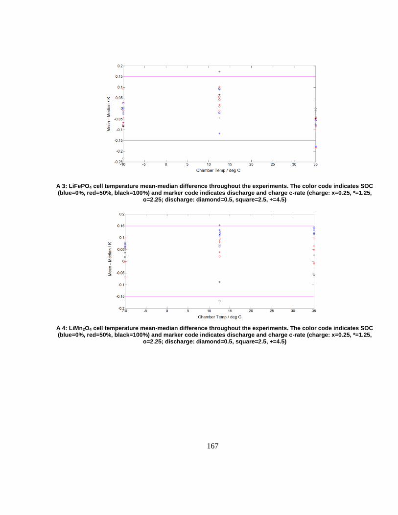
167
A 3: LiFePO4 cell temperature mean-median difference throughout the experiments. The color code indicates SOC (blue=0%, red=50%, black=100%) and marker code indicates discharge and charge c-rate (charge: x=0.25, *=1.25,
o=2.25; discharge: diamond=0.5, square=2.5, +=4.5)
A 4: LiMn2O4 cell temperature mean-median difference throughout the experiments. The color code indicates SOC (blue=0%, red=50%, black=100%) and marker code indicates discharge and charge c-rate (charge: x=0.25, *=1.25,
o=2.25; discharge: diamond=0.5, square=2.5, +=4.5)

168
Appendix-B
Derived Regression Models for the Circuit Parameters
Battery #1 (LFP Cathode):
if (8.5<=temp)&&(temp<16.5)
R1= -1.1924E-11*SOC^4 + 3.4367E-09*SOC^3 - 2.9815E-07*SOC^2 + 8.3662E- 06*SOC^1 + 9.0340E-04;
R2=-7.3164E-12*SOC^4 + 5.8531E-10*SOC^3 - 2.0011E-09*SOC^2 - 7.9285E-07*SOC^1 + 1.6792E-03;
C1= -7.2415E-07*SOC^4 + 1.9663E-04*SOC^3 - 1.6592E-02*SOC^2 + 4.7056E-01*SOC^1 + 1.8084E+01;
C2= -9.3682E-05*SOC^4 + 2.2157E-02*SOC^3 - 1.7448E+00*SOC^2 + 5.1351E+01*SOC^1 + 3.6988E+01;
R3=-2.8547E-09*SOC^3 + 4.0633E-07*SOC^2 - 1.6189E-05*SOC^1 + 9.2442E-04;
R4=7.6329E-11*SOC^4 - 1.4614E-08*SOC^3 + 9.3078E-07*SOC^2 - 2.1735E-05*SOC^1 + 5.0689E-04;
C3= -1.3139E-03*SOC^4 + 2.8153E-01*SOC^3 - 2.1037E+01*SOC^2 + 5.9944E+02*SOC^1 + 9.4176E+03;
R5=-8.2231E-09*SOC^3 + 1.3670E-06*SOC^2 - 7.0295E-05*SOC^1 + 4.6949E-03;
C4=-1.3881E-02*SOC^4 + 2.7501E+00*SOC^3 - 1.8106E+02*SOC^2 + 4.5201E+03*SOC^1 + 2.5236E+04;
elseif (16.5<=temp)&&(temp<32)
R1=-7.3624E-12*SOC^4 + 9.8197E-10*SOC^3 - 5.5139E-08*SOC^2 + 3.4816E-06*SOC^1 + 6.9355E-04;
R2=5.3921E-12*SOC^4 - 1.1286E-09*SOC^3 + 1.1558E-07*SOC^2 - 8.4552E-06*SOC^1 + 8.7765E-04;
C1= -1.2508E-06*SOC^4 + 1.9713E-04*SOC^3 - 1.1057E-02*SOC^2 + 4.6085E-01*SOC^1 + 1.8513E+01;
C2=2.3234E-05*SOC^4 - 6.0979E-03*SOC^3 + 4.0664E-01*SOC^2 + 1.8484E+00*SOC^1 + 4.4622E+02;
R3=4.8039E-12*SOC^4 - 1.4603E-09*SOC^3 + 1.6947E-07*SOC^2 - 9.1099E-06*SOC^1 + 4.5446E-04;
R4=-4.4560E-12*SOC^4 + 6.4079E-10*SOC^3 + 9.0600E-10*SOC^2 - 2.5548E-06*SOC^1 + 2.5477E-04;
C3=2.9485E-03*SOC^4 - 6.5496E-01*SOC^3 + 4.5311E+01*SOC^2 - 9.8769E+02*SOC^1 + 2.1574E+04;
R5=2.7156E-10*SOC^4 - 6.5474E-08*SOC^3 + 5.6005E-06*SOC^2 - 1.9843E-04*SOC^1 + 4.7122E-03;
C4=-4.4313E-04*SOC^4 + 1.2049E-01*SOC^3 - 1.5526E+01*SOC^2 + 9.4699E+02*SOC^1 + 5.4311E+04;
elseif (31<=temp)&&(temp<45)
R1= 1.3499E-09*SOC^3 - 2.6207E-07*SOC^2 + 1.5019E-05*x + 6.5366E-04;
R2= -8.2144E-10*SOC^3 + 1.5712E-07*SOC^2 - 9.7821E-06*x + 2.9033E-04;
R3= 1.2436E-10*SOC^3 - 2.5186E-08*SOC^2 + 1.5903E-06*x + 1.1561E-04;
R4= 9.2859E-09*SOC^3 - 8.4466E-07*SOC^2 + 1.8849E-05*x + 1.5014E-04;
R5= -3.2258E-08*SOC^3 + 4.6544E-06*SOC^2 - 2.1509E-04*x + 5.3658E-03;
C1= 3.2702E-04*SOC^4 - 5.7252E-02*SOC^3 + 2.8252E+00*SOC^2 - 1.4737E+01*x + 7.3334E+01;

169
C2= 5.5117E-02*SOC^3 - 1.0919E+01*SOC^2 + 6.4710E+02*x + 3.8183E+02;
C3= 2.4611E-01*SOC^3 - 2.3601E+01*SOC^2 + 6.6653E+02*x + 6.7549E+04;
C4= -2.2639E-01*SOC^3 + 1.9599E+01*SOC^2 - 1.6303E+02*x + 9.9379E+04;
end
Battery #2, (LMO & NMC Cathode):
if (temp>=8)&&(temp<=18)
R1= 7.0808E-08*SOC^2 - 5.8329E-06*x + 1.3915E-03;
R2= 4.2228E-08*SOC^2 - 3.7060E-06*x + 8.5987E-04;
C1= 1.1364E-02*SOC^2 - 9.1497E-01*x + 4.4608E+01;
C2 = -1.8337E-03*SOC^3 + 2.3421E-01*SOC^2 - 7.1334E+00*x + 2.7454E+02;
R3=-8.0898E-09*SOC^3 + 1.5283E-06*SOC^2 - 1.0322E-04*x + 2.9054E-03;
R4=-3.1205E-09*SOC^3 + 5.6908E-07*SOC^2 - 3.1298E-05*x + 6.9424E-04;
C3= 1.2041E-01*SOC^3 - 2.6735E+01*SOC^2 + 1.5754E+03*x - 2.4632E+03;
R5= -4.3900E-08*SOC^3 + 6.5245E-06*SOC^2 - 2.7019E-04*x + 6.5161E-03;
C4= 5.3293E-01*SOC^3 - 8.0547E+01*SOC^2 + 3.3463E+03*x + 2.5908E+04;
else if (temp>=18)&&(temp<=28)
R1= -2.6762E-10*SOC^4 + 5.1171E-08*SOC^3 - 3.2003E-06*SOC^2 + 7.5197E-05*x + 4.8916E-04;
R2=-1.8426E-11*SOC^4 + 1.2486E-09*SOC^3 + 1.1699E-07*SOC^2 - 9.4292E-06*x + 6.9954E-04;
C1=-1.6493E-05*SOC^4 + 3.1013E-03*SOC^3 - 1.8869E-01*SOC^2 + 4.4103E+00*x - 1.0525E+01;
C2=-9.2389E-05*SOC^4 + 1.6293E-02*SOC^3 - 9.6568E-01*SOC^2 + 2.3868E+01*x + 1.9789E+01;
R3=-4.1093E-09*SOC^3 + 8.7954E-07*SOC^2 - 6.1557E-05*x + 1.4540E-03;
R4=8.3556E-11*SOC^4 - 1.7391E-08*SOC^3 + 1.2093E-06*SOC^2 - 3.1617E-05*x + 3.9427E-04;
C3=1.5092E-02*SOC^4 - 2.9776E+00*SOC^3 + 1.9159E+02*SOC^2 - 4.5309E+03*x + 6.5452E+04;
R5=-1.4079E-10*SOC^4 - 9.9293E-09*SOC^3 + 3.5492E-06*SOC^2 - 1.5901E-04*x + 4.5593E-03;
C4=-6.2102E-02*SOC^4 + 1.2514E+01*SOC^3 - 8.4189E+02*SOC^2 + 2.1587E+04*x - 1.0310E+05;
else if (temp>28)
R1= -3.1405E-09*SOC^3 + 4.6714E-07*SOC^2 - 1.8254E-05*x + 1.2772E-03;
R2= 2E-10*SOC^4 - 4E-08*SOC^3 + 3E-06*SOC^2 - 8E-05*x + 0.0008;
C1= -1.5376E+00*SOC^2 + 3.1609E+02*x - 2.8505E+03;
C2= 5.2240E-03*SOC^3 - 3.7153E+00*SOC^2 + 5.5959E+02*x + 1.4230E+03;
R3=-4.4305E-09*SOC^3 + 6.6673E-07*SOC^2 - 2.5507E-05*x + 3.9728E-04;

170
R4= -7.1244E-08*SOC^3 + 8.8381E-06*SOC^2 - 2.6090E-04*x + 4.4370E-03;
C3=1.7719E-01*SOC^3 - 3.5050E+01*SOC^2 + 1.7530E+03*x + 7.3067E+04;
R5=1.6885E-09*SOC^3 + 5.3492E-07*SOC^2 - 4.3545E-05*x + 1.0523E-03;
C4= 1.0117E+00*SOC^3 - 1.1603E+02*SOC^2 + 3.5250E+03*x + 3.7591E+04;
End

B-1
Appendix-C
Modification on the driver model in Autonomie to take in the power demand as
input
C 1: driver sub-model- top level
C 2: Torque demand estimator

B-1
Appendix-D
Monthly Report of EV-ACX2.5
October 2011
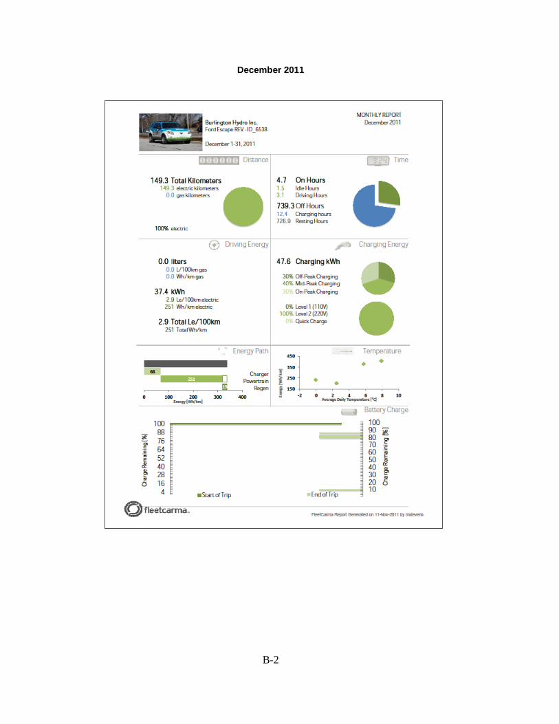
B-2
December 2011

B-3
January 2012
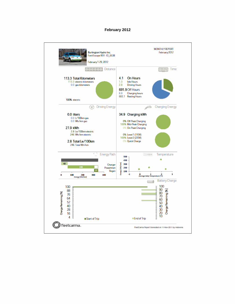
February 2012