Full Terms & Conditions of access and use can be found athttps://www.tandfonline.com/action/journalInformation?journalCode=tcfm20

Engineering Applications of Computational FluidMechanics

ISSN: 1994-2060 (Print) 1997-003X (Online) Journal homepage: https://www.tandfonline.com/loi/tcfm20

Modeling monthly pan evaporation using waveletsupport vector regression and wavelet artificialneural networks in arid and humid climates

Sultan Noman Qasem, Saeed Samadianfard, Salar Kheshtgar, Salar Jarhan,Ozgur Kisi, Shahaboddin Shamshirband & Kwok-Wing Chau

To cite this article: Sultan Noman Qasem, Saeed Samadianfard, Salar Kheshtgar, Salar Jarhan,Ozgur Kisi, Shahaboddin Shamshirband & Kwok-Wing Chau (2019) Modeling monthly panevaporation using wavelet support vector regression and wavelet artificial neural networks in aridand humid climates, Engineering Applications of Computational Fluid Mechanics, 13:1, 177-187,DOI: 10.1080/19942060.2018.1564702

To link to this article: https://doi.org/10.1080/19942060.2018.1564702

© 2019 The Author(s). Published by InformaUK Limited, trading as Taylor & FrancisGroup

Published online: 11 Jan 2019.

Submit your article to this journal

Article views: 140

View Crossmark data

ENGINEERING APPLICATIONS OF COMPUTATIONAL FLUID MECHANICS2019, VOL. 13, NO. 1, 177–187https://doi.org/10.1080/19942060.2018.1564702

Modeling monthly pan evaporation using wavelet support vector regression andwavelet artificial neural networks in arid and humid climates

Sultan Noman Qasema,b, Saeed Samadianfardc, Salar Kheshtgard, Salar Jarhane, Ozgur Kisif ,Shahaboddin Shamshirbandg,h and Kwok-Wing Chaui

aComputer Science Department, College of Computer and information Sciences, Al ImamMohammad Ibn Saud Islamic University (IMSIU),Riyadh, Saudi Arabia; bComputer Science Department, Faculty of Applied Sciences, Taiz University, Taiz, Yemen; cDepartment of WaterEngineering, University of Tabriz, Tabriz, Iran; dDepartment of Building, Civil and Environmental Engineering, Faculty of Engineering andComputer Science, Concordia University, Montreal, Canada; eDepartment of Hydrosciences, Technische Univeristät Dresden, Dresden, Germany;fFaculty of Natural Sciences and Engineering, Ilia State University, Tbilisi, Georgia; gDepartment for Management of Science and TechnologyDevelopment, Ton Duc Thang University, Ho Chi Minh City, Vietnam; hFaculty of Information Technology, Ton Duc Thang University, Ho Chi MinhCity, Vietnam; iDepartment of Civil and Environmental Engineering, Hong Kong Polytechnic University, Hong Kong, People’s Republic of China

ABSTRACTEvaporation rate is one of the key parameters in determining the ecological conditions and it hasan irrefutable role in the proper management of water resources. In this paper, the efficiency ofsomedata-driven techniques including support vector regression (SVR) andartificial neural networks(ANN) and combination of them with wavelet transforms (WSVR and WANN) were investigated forpredicting evaporation rates at Tabriz (Iran) and Antalya (Turkey) stations. For evaluating the perfor-mances of studied techniques, four different statistical indicatorswere utilizednamely the rootmeansquareerror (RMSE), themeanabsolute error (MAE), the correlation coefficient (R), andNash–Sutcliffeefficiency (NSE). Additionally, Taylor diagrams were implemented to test the similarity among theobserved and predicted data. Outcomes showed that at Tabriz station, the ANN3 (third input com-bination that are air temperatures and solar radiation used by ANN) with RMSE of 0.701, MAE of0.525, R of 0.990 and NSE of 0.977 had better performances in comparison with WANN, SVR andWSVR. So, the wavelet transforms did not have positive effects in increasing the precision of ANNand SVR predictions at Tabriz station. Also, approximately the same trend was seen at Antalya sta-tion. In other words, ANN5 (fifth input combination that are air temperatures, relative humidity andsolar radiationusedbyANN)with RMSEof 0.923,MAEof 0.697,Rof 0.962 andNSEof 0.898hadamoreaccurate predictions among others. Conversely, wavelet transform reduced the prediction errors ofSVR at Antalya station. So, the WSVR5 with RMSE of 1.027, MAE of 0.728, R of 0.950 and NSE of 0.870predicted evaporation rates of Antalya station more precisely than other SVR models. As a conclu-sion, results from the current study proved that ANN provided reasonable trends for evaporationmodeling at both Tabriz and Antalya stations.

ARTICLE HISTORYReceived 24 October 2018Accepted 28 December 2018

KEYWORDSData-driven technique;estimation; meteorologicalparameters; pan evaporation

1. Introduction

Evaporation is playing a prominent role in the processesof hydrologic cycle. Therefore, estimation of this phe-nomenon is necessary as it affects water resources, espe-cially in arid and semi-arid areas like Iran. A considerableamount of precipitation is allocated to evaporation andthe sum of evaporation from the land surface is approx-imately 61% of the entire global precipitation (Chow,Maidment, & Mays, 1988). Every year, several millionsof cubic meters of fresh water that has collected withhigh costs, efforts and difficulties evaporated from tankof dams and reservoirs. Therefore, it is of great signif-icance to estimate the evaporation amount for water

CONTACT Shahaboddin Shamshirband shahaboddin.shamshirband@tdtu.edu.vn

resource monitoring. In regions with hot weather andlow rainfall, evaporation can lead to losing the notice-able amount of water, hence it causes decreasing in thewater surface elevation. Typically, there are two differ-ent (direct and indirect) approaches for estimation ofevaporation from various variables. Measuring pan is themost prevalent direct method for specifying the value ofevaporation (Stanhill, 2002). Class A pan, as themost fre-quently used pan, has 4 ft (122 cm) in diameter and 10inch (25 cm) deep and is located about 6 inch (15 cm)above the soil surface. Although calculating evapora-tion by using pans appears to be having precise answersbut using indirect approaches for approximating pan

© 2019 The Author(s). Published by Informa UK Limited, trading as Taylor & Francis GroupThis is an Open Access article distributed under the terms of the Creative Commons Attribution License (http://creativecommons.org/licenses/by/4.0/), which permits unrestricted use,distribution, and reproduction in any medium, provided the original work is properly cited.

178 S. N. QASEM ET AL.

evaporation (PE) seems to be easier and cost-effectivedue to the fact that installing pans and meteorologicalstations are the expensive process. Indirect methods forestimation of PE are based on using meteorological vari-ables. Empirical and semi-empirical models have beencompletely used for calculating PE from meteorologi-cal variables such as wind speed, sunshine hours, rel-ative humidity, radiation, atmosphere pressure and themain factor, temperature. Because of these several vari-ables, estimating evaporation rate becomes more com-plex as it is totally non-linear. A number of scholarshave tried to predict evaporation from different mete-orological variables (Chang, Sun, & Chung, 2013; Kisi,2006; Lin, Lin, & Wu, 2013). In recent years, machinelearning approaches including Artificial Neural Net-work (ANN), Adaptive Neuro-Fuzzy Inference System(ANFIS), Fuzzy Genetic (FG), Support Vector Regres-sion (SVR) and the integrated models of these methodswithwavelet or other data preprocessing approaches havebeen effectively applied in water related fields such aswater resource engineering, prediction of suspended sed-iment load in rivers, forecasting monthly stream flow,estimating friction factor in irrigation pipes, PE mod-eling, etc. (Chau, 2017; Choubin et al., 2018; Choubin,Malekian, Samadi, Khalighi Sigaroodi, & Sajedi Hosseini,2017; Fotovatikhah et al., 2018; Jain & Srinivasulu, 2004;Keshtegar, Piri, & Kisi, 2016; Kisi, 2005; Kisi, Genc, Dinc,&Zounemat-Kermani, 2016; Nourani, Alami, &Danesh-var Vousoughi, 2015; Rajaee, Mirbagheri, Zounemat-Kermani, & Nourani, 2009; Samadianfard et al., 2018;Samadianfard, Delirhasannia, Kisi, & Agirre-Basurko,2013; Samadianfard, Nazemi, & Sadraddini, 2014; Sama-dianfard, Sattari, Kisi, & Kazemi, 2014; Taormina, Chau,& Sivakumar, 2015; Wang, Xu, Chau, & Chen, 2013).Goyal, Bharti, Quilty, Adamowski, and Pandey (2014)applied ANN, ANFIS, least squares-SVR (LS-SVR) andfuzzy logic to increase the precision of PE estimationusing various meteorological variables, like daily rain-fall, sunshine hours, minimum and maximum air tem-peratures and humidity. The outcomes exhibited thatthe LS-SVR and fuzzy logic can be utilized effectivelyin predicting PE values. Guven and Kisi (2013) com-pared the precision of five different models in model-ing PE named: ANFIS, ANN, FG, Stephens–Stewart (SS)and Linear Genetic Programming (LGP) methods. Theresults revealed that LGP model has a better accuracy incomparison to other models and can be utilized success-fully to estimate PE. Kisi and Tombul (2013) applied theFG method in estimation of PE in two different stationsinside Turkey and compared the accuracy of the methodwith the ANFIS, ANN and SS approaches. Finally, it wasconcluded that the FG method has the closest estima-tion in comparison to other models. Tabari, Marofi, and

Sabziparvar (2009) examined the precision of ANN andMultivariate Non-Linear Regression (MNLR) methodsfor PE estimation in a semi-arid area. The consequencesindicated that theANNapproach provided the finest esti-mates of PE. ANN and genetic algorithms were utilizedby Kim and Kim (2008) for PE and evapotranspirationmodeling. The outcomes indicated the specific capabili-ties of both studiedmodels for the precise approximationof PE and evapotranspiration values. Recently, Shafaeiand Kisi (2015) applied ANFIS, SVR and autoregres-sive moving average (ARMA) models, separately, thencombined the models with wavelet, known as WAN-FIS, WSVR, and WARMA models. The efficiency of theaforementioned two groups (single form of models andcombined forms) is compared with each other. Obtainedresults discovered that the combined models give betteraccuracy in anticipating lake levels in the study zone incomparison to single models.

In previous researches, it has been tried to improve theprediction accuracy of PE estimates. So, it can be com-prehended that the current gap is developing and imple-menting new methods for decreasing the predictionerrors. So, in the current research, the potential of twomachine learning approaches, namely ANN and SVR,and the integrated wavelet of these models, Wavelet-ANN (WANN) andWavelet-SVR (WSVR), used to fore-cast evaporation rates in Tabriz and Antalya stations andthe efficiencies of them were compared with each other.The goals of the study were (i) evaluating the perfor-mance of aforementioned models in the estimation ofPE, and (ii) investigating the role of climate in predict-ing PE by considering humid and arid climates. The restof the paper is structured as follow. Section 2 providesthe characteristics of study area, description of imple-mented methods and evaluation parameters. Addition-ally, section 3 discussed the obtained results and finally,the conclusion is presented in section 4.

2. Materials andmethods

2.1. Study area

The monthly data of two synoptic stations in two differ-ent countries, Tabriz Station (latitude 38°05′N, longitude46°17′E) in Iran and Antalya Station (latitude 36°42′N,longitude 30°44′E) in Turkey that are in approximatelysame latitudes, were used in the current study (Figure 1).Tabriz, which is situated at northwestern of Iran, is amountainous basin with a semi-arid climate and coldwinters. Besides, Antalya, which is placed in the south-ern region of Turkey, has Mediterranean climate thatcharacterized by temperate wet winters and hot arid sum-mer. The elevations from sea level are 1350 and 64 m

ENGINEERING APPLICATIONS OF COMPUTATIONAL FLUID MECHANICS 179

Figure 1. The location of Tabriz and Antalya stations (URL1).

Table 1. The monthly statistical parameters of each meteorological station.

Statistic T (°C) RH (%) W (m/s) Rs (MJ/m2 day) PE (mm)

Station Tabriz Antalya Tabriz Antalya Tabriz Antalya Tabriz Antalya Tabriz Antalya

Minimum −6.474 7.800 25.137 45.500 1.117 1.800 6.243 5.588 0.000 1.600Maximum 28.769 32.250 82.460 67.500 5.617 4.900 30.008 30.245 15.448 12.400Mean 13.092 19.874 51.058 55.800 3.385 2.756 18.011 17.608 5.425 5.568Standard deviation 9.848 7.327 14.406 4.223 0.934 0.517 7.220 6.523 4.956 2.672Variation coefficient 0.751 0.368 0.282 0.076 0.275 0.187 0.400 0.370 0.912 0.479Skewness −0.064 −0.001 0.181 0.123 0.161 0.817 0.022 −0.132 0.299 0.455Kurtosis −1.322 −1.408 −1.193 −0.219 −0.553 1.206 −1.403 −1.262 −1.358 −0.887Correlation with PE 0.963 0.912 −0.892 −0.342 0.730 −0.269 0.927 0.843 1.000 1.000

for the Tabriz and Antalya stations, respectively. In sum-mary, as it can be proved from Table 1, Antalya has ahot and wet climate. In contrary, Tabriz has cold and dryweather. Meteorological variables that were used for thisstudy are air temperatures (T), solar radiation (Rs), windspeed (W), relative humidity (RH) and PE with the timeperiod of 1992–2016 for Tabriz station and 1986–2006 forAntalya station. Table 1 represents the monthly statisticalparameters of the applied variables for both stations. Itcan be seen in Table 1 that themean values of PE at Tabrizand Antalya stations are 5.425 and 5.568mm, respec-tively. Furthermore, it is obvious that the minimum PEin Tabriz station is zero because in winters when the tem-perature reaches below zero, water freezes in the pan andthe volume of evaporation becomes negligible. Most ofthe variables indicate normal distributions because theyhave low skewness values, except wind speed in Antalyastation which has the maximum skewness and shows askewed distribution. This might be due to the location ofthis station in a coastal area (Kisi, 2009). Correlations aregenerally higher for the Tabriz station and temperatureand PE show a higher variation in Tabriz when compared

to Antalya. Table 1 also shows the correlations betweenPE and other parameters. In both stations, T and Rs havefirst and second high correlations with PE, respectively.Moreover, the highest inverse correlations are betweenRH and PE in both stations. The observed PE data forboth Tabriz and Antalya stations are shown in Figure 2.

2.2. Artificial neural networks

In preceding decades, the ANN approach was con-sidered by many researchers as a dependable tool ofcomputations. From the initial neural model whichhas been introduced by McCulloch and Pitts (1943),researchers developed several different models. Addi-tionally, most activities have been concentrated on back-propagation and its extensions (Salas, Markus, & Tokar,2000). This algorithm (Rumelhart & McClelland, 1986)is utilized in feed-forward ANNs, meaning that the neu-rons are ordered in several layers, and deliver their sig-nals forward, then the errors are propagated backward.The network obtains inputs by input layer neurons, andthe network output is obtained from the output layer

180 S. N. QASEM ET AL.

Figure 2. The observed PE for Tabriz and Antalya stations.

Figure 3. The typical configuration of the ANNmodel.

neurons. The number of hidden layers is typically deter-mined by trial and error. ANNs are extremely talented ofmodeling and simulating linear and non-linear systems.In the current study, input layers were determined usinga trial-error process and the number of neurons in eachlayer were selected to be among 1 and 10. Figure 3 showsa typical configuration of the ANNmodel.

2.3. Support vector regression

The support vectormachine (SVM) is an extensively usedand popular estimator which its fundamental idea wasintroduced by Vapnik (1995, 1998). Then, a regressiontechnique, namely SVR, was developed based on SVMmodels in order to solve complex problems, effectively.This model was constructed on the structural risk mini-mization. For this purpose, ε− the insensitive loss func-tion is identified which means that the model allows tol-erating errors up to ε in the training data sets. Therefore,

the SVR seeks for a linear function formulated as follows:

P(x) = FTx + L, (1)

where F and L denote the coefficients of the weight vectorof the linear expression. This linear regression problemcan be explained as the following optimization problem:

Min12||F||2 + C

N∑i=1

(ξi + ξ∗i ) Subject to

×

⎧⎪⎨⎪⎩FTx + L − yi ≤ ε + ξ∗

iyi − FTx − L ≤ ε + ξi

ξi, ξ∗i ≥ 0, i = 1, 2, . . . ,N

. (2)

The constant C > 0 is a positive trade-off factor forthe grade of the experimental error. C and ε are prede-fined parameters. Moreover, ξi and ξ∗

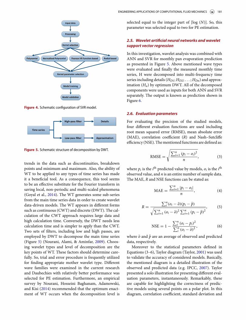
i that is called asslack variables. For solving this problem, the SVR useskernel trick (Smola & Scholkopf, 2004). In this study,four different kernel functions, including Pearson VIIfunction-based, radial basis function (RBF), polynomialand normalized polynomial are used. For building opti-mum SVRmodel, the parameters of SVR such as the ker-nel function,C and εmust be selected cautiously. Figure 4indicates the schematic configuration of the SVR model.

2.4. Wavelet transform

Developed by Grossman and Morlet (1984), the wavelettransform (WT) has been broadly applied in differ-ent fields of science and engineering. It is mathemati-cal transformations which are used for eliciting furtherinformation from the data which is not currently obvi-ous in its crude form. This transformation can determine

ENGINEERING APPLICATIONS OF COMPUTATIONAL FLUID MECHANICS 181

Figure 4. Schematic configuration of SVR model.

Figure 5. Schematic structure of decomposition by DWT.

trends in the data such as discontinuities, breakdownpoints and minimum and maximum. Also, the ability ofWT to be applied to any types of time series has madeit a beneficial tool. As a consequence, this tool seemsto be an effective substitute for the Fourier transform insaving local, non-periodic and multi-scaled phenomena(Goyal et al., 2014). The WT generates some sub-seriesfrom the main time series data in order to create waveletdata-driven models. The WT appears in different formssuch as continuous (CWT) and discrete (DWT). The cal-culation of the CWT approach requires large data andhigh calculation time. Conversely, the DWT needs lesscalculation time and is simpler to apply than the CWT.Two sets of filters, including low and high passes, areemployed by DWT to decompose the main time series(Figure 5) (Nourani, Alami, & Aminfar, 2009). Choos-ing wavelet types and level of decomposition are thekey points of WT. These factors should determine care-fully. So, trial and error procedure is frequently utilizedfor finding appropriate mother wavelet type. Differentwave families were examined in the current researchand Daubechies with relatively better performance wasselected for PE estimation. Furthermore, an empiricalsurvey by Nourani, Hosseini Baghanam, Adamowski,and Kisi (2014) recommended that the optimum enact-ment of WT occurs when the decomposition level is

selected equal to the integer part of [log (N)]. So, thisparameter was selected equal to two for PE estimation.

2.5. Wavelet artificial neural networks andwaveletsupport vector regression

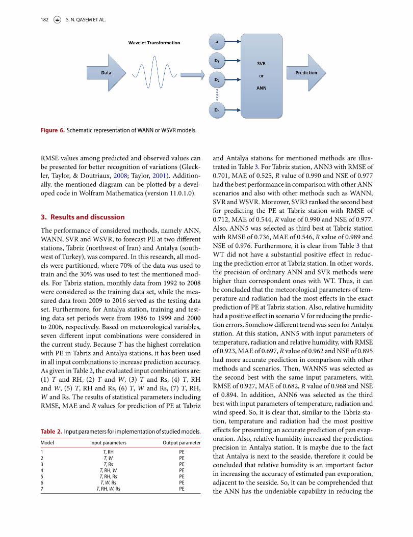
In this investigation, wavelet analysis was combined withANN and SVR for monthly pan evaporation predictionas presented in Figure 5. Above mentioned wave typeswere evaluated and finally the measured monthly timeseries, H were decomposed into multi-frequency timeseries including details (HD1;HD2; . . . ;HDn) and approx-imation (Ha) by optimum DWT. All of the decomposedcomponents were used as inputs for both ANN and SVRseparately. The output is known as prediction shown inFigure 6.

2.6. Evaluation parameters

For evaluating the precision of the studied models,four different evaluation functions are used includingroot mean squared error (RMSE), mean absolute error(MAE), correlation coefficient (R) and Nash–Sutcliffeefficiency (NSE). Thementioned functions are defined as:

RMSE =√∑n

i=1 (pi − oi)2

n, (3)

where pi is the ith predicted value by models, oi is the ithobserved value, and n is an entire number of sample data.The MAE, R and NSE functions can be stated as:

MAE =∑n

i=1 |pi − oi|n

, (4)

R =∑n

i (oi − o)(pi − p)√∑ni=1 (oi − o)2

∑ni=1 (pi − p)2

, (5)

NSE = 1 −∑n

i (oi − pi)2∑ni (oi − o)2

, (6)

where o and p are an average of observed and predicteddata, respectively.

Moreover to the statistical parameters defined inEquations (3–6), Taylor diagram (Taylor, 2001) was usedto validate the accuracy of considered models. Basically,the mentioned diagram is a detailed illustration of theobserved and predicted data (e.g. IPCC, 2007). Taylorpresented a solo illustration for presenting different eval-uation parameters, instantaneously. Remarkably, theseare capable for highlighting the correctness of predic-tive models using several points on a polar plot. In thisdiagram, correlation coefficient, standard deviation and

182 S. N. QASEM ET AL.

Figure 6. Schematic representation of WANN or WSVR models.

RMSE values among predicted and observed values canbe presented for better recognition of variations (Gleck-ler, Taylor, & Doutriaux, 2008; Taylor, 2001). Addition-ally, the mentioned diagram can be plotted by a devel-oped code in Wolfram Mathematica (version 11.0.1.0).

3. Results and discussion

The performance of considered methods, namely ANN,WANN, SVR and WSVR, to forecast PE at two differentstations, Tabriz (northwest of Iran) and Antalya (south-west of Turkey), was compared. In this research, all mod-els were partitioned, where 70% of the data was used totrain and the 30% was used to test the mentioned mod-els. For Tabriz station, monthly data from 1992 to 2008were considered as the training data set, while the mea-sured data from 2009 to 2016 served as the testing dataset. Furthermore, for Antalya station, training and test-ing data set periods were from 1986 to 1999 and 2000to 2006, respectively. Based on meteorological variables,seven different input combinations were considered inthe current study. Because T has the highest correlationwith PE in Tabriz and Antalya stations, it has been usedin all input combinations to increase prediction accuracy.As given in Table 2, the evaluated input combinations are:(1) T and RH, (2) T and W, (3) T and Rs, (4) T, RHand W, (5) T, RH and Rs, (6) T, W and Rs, (7) T, RH,W and Rs. The results of statistical parameters includingRMSE, MAE and R values for prediction of PE at Tabriz

Table 2. Inputparameters for implementationof studiedmodels.

Model Input parameters Output parameter

1 T, RH PE2 T,W PE3 T, Rs PE4 T, RH,W PE5 T, RH, Rs PE6 T,W, Rs PE7 T, RH,W, Rs PE

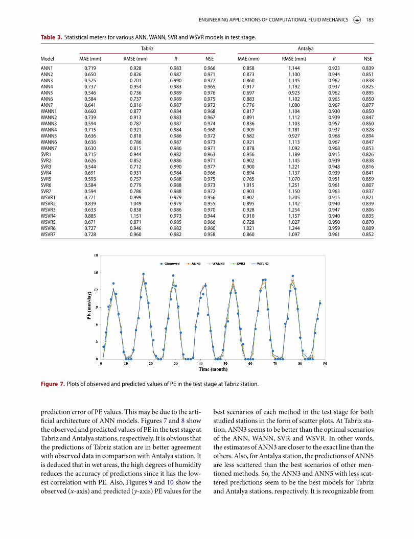
and Antalya stations for mentioned methods are illus-trated in Table 3. For Tabriz station, ANN3with RMSE of0.701, MAE of 0.525, R value of 0.990 and NSE of 0.977had the best performance in comparisonwith otherANNscenarios and also with other methods such as WANN,SVR andWSVR.Moreover, SVR3 ranked the second bestfor predicting the PE at Tabriz station with RMSE of0.712, MAE of 0.544, R value of 0.990 and NSE of 0.977.Also, ANN5 was selected as third best at Tabriz stationwith RMSE of 0.736, MAE of 0.546, R value of 0.989 andNSE of 0.976. Furthermore, it is clear from Table 3 thatWT did not have a substantial positive effect in reduc-ing the prediction error at Tabriz station. In other words,the precision of ordinary ANN and SVR methods werehigher than correspondent ones with WT. Thus, it canbe concluded that the meteorological parameters of tem-perature and radiation had the most effects in the exactprediction of PE at Tabriz station. Also, relative humidityhad a positive effect in scenarioV for reducing the predic-tion errors. Somehowdifferent trendwas seen forAntalyastation. At this station, ANN5 with input parameters oftemperature, radiation and relative humidity, with RMSEof 0.923,MAE of 0.697,R value of 0.962 andNSE of 0.895had more accurate prediction in comparison with othermethods and scenarios. Then, WANN5 was selected asthe second best with the same input parameters, withRMSE of 0.927, MAE of 0.682, R value of 0.968 and NSEof 0.894. In addition, ANN6 was selected as the thirdbest with input parameters of temperature, radiation andwind speed. So, it is clear that, similar to the Tabriz sta-tion, temperature and radiation had the most positiveeffects for presenting an accurate prediction of pan evap-oration. Also, relative humidity increased the predictionprecision in Antalya station. It is maybe due to the factthat Antalya is next to the seaside, therefore it could beconcluded that relative humidity is an important factorin increasing the accuracy of estimated pan evaporation,adjacent to the seaside. So, it can be comprehended thatthe ANN has the undeniable capability in reducing the

ENGINEERING APPLICATIONS OF COMPUTATIONAL FLUID MECHANICS 183

Table 3. Statistical meters for various ANN, WANN, SVR and WSVR models in test stage.

Tabriz Antalya

Model MAE (mm) RMSE (mm) R NSE MAE (mm) RMSE (mm) R NSE

ANN1 0.719 0.928 0.983 0.966 0.858 1.144 0.923 0.839ANN2 0.650 0.826 0.987 0.971 0.873 1.100 0.944 0.851ANN3 0.525 0.701 0.990 0.977 0.860 1.145 0.962 0.838ANN4 0.737 0.954 0.983 0.965 0.917 1.192 0.937 0.825ANN5 0.546 0.736 0.989 0.976 0.697 0.923 0.962 0.895ANN6 0.584 0.737 0.989 0.975 0.883 1.102 0.965 0.850ANN7 0.641 0.816 0.987 0.972 0.776 1.000 0.967 0.877WANN1 0.660 0.877 0.984 0.968 0.817 1.104 0.930 0.850WANN2 0.739 0.913 0.983 0.967 0.891 1.112 0.939 0.847WANN3 0.594 0.787 0.987 0.974 0.836 1.103 0.957 0.850WANN4 0.715 0.921 0.984 0.968 0.909 1.181 0.937 0.828WANN5 0.636 0.818 0.986 0.972 0.682 0.927 0.968 0.894WANN6 0.636 0.786 0.987 0.973 0.921 1.113 0.967 0.847WANN7 0.630 0.815 0.986 0.971 0.878 1.092 0.968 0.853SVR1 0.715 0.944 0.982 0.963 0.956 1.189 0.915 0.826SVR2 0.626 0.852 0.986 0.971 0.902 1.145 0.939 0.838SVR3 0.544 0.712 0.990 0.977 0.900 1.221 0.948 0.816SVR4 0.691 0.931 0.984 0.966 0.894 1.137 0.939 0.841SVR5 0.593 0.757 0.988 0.975 0.765 1.070 0.951 0.859SVR6 0.584 0.779 0.988 0.973 1.015 1.251 0.961 0.807SVR7 0.594 0.786 0.988 0.972 0.903 1.150 0.963 0.837WSVR1 0.771 0.999 0.979 0.956 0.902 1.205 0.915 0.821WSVR2 0.839 1.049 0.979 0.955 0.895 1.142 0.940 0.839WSVR3 0.633 0.838 0.986 0.970 0.928 1.254 0.947 0.806WSVR4 0.885 1.151 0.973 0.944 0.910 1.157 0.940 0.835WSVR5 0.671 0.871 0.985 0.966 0.728 1.027 0.950 0.870WSVR6 0.727 0.946 0.982 0.960 1.021 1.244 0.959 0.809WSVR7 0.728 0.960 0.982 0.958 0.860 1.097 0.961 0.852

Figure 7. Plots of observed and predicted values of PE in the test stage at Tabriz station.

prediction error of PE values. Thismay be due to the arti-ficial architecture of ANN models. Figures 7 and 8 showthe observed and predicted values of PE in the test stage atTabriz andAntalya stations, respectively. It is obvious thatthe predictions of Tabriz station are in better agreementwith observed data in comparisonwithAntalya station. Itis deduced that in wet areas, the high degrees of humidityreduces the accuracy of predictions since it has the low-est correlation with PE. Also, Figures 9 and 10 show theobserved (x-axis) and predicted (y-axis) PE values for the

best scenarios of each method in the test stage for bothstudied stations in the form of scatter plots. At Tabriz sta-tion, ANN3 seems to be better than the optimal scenariosof the ANN, WANN, SVR and WSVR. In other words,the estimates of ANN3 are closer to the exact line than theothers. Also, forAntalya station, the predictions ofANN5are less scattered than the best scenarios of other men-tioned methods. So, the ANN3 and ANN5 with less scat-tered predictions seem to be the best models for Tabrizand Antalya stations, respectively. It is recognizable from

184 S. N. QASEM ET AL.

Figure 8. Plots of observed and predicted values of PE in the test stage at Antalya station.

Figure 9. Scatter plots of considered models for PE estimation in the test stage at Tabriz station.

Figure 10. Scatter plots of considered models for PE estimation in the test stage at Antalya station.

Figure 10 that in Antalya station, asmuch as the observedamount of evaporation increases, the estimated amountdeviates from the exact line. So, estimation of evapo-ration for great values has less accuracy in comparisonto low values. However, Figure 9 shows that for Tabrizstation this deviation is not noticeable. Moreover, theresulted statistical parameters of the mentioned modelsin the test period are presented in Table 3. Additionally,the overall results proved that the accuracy of the studiedmodels in Tabriz station was higher than Antalya sta-tion. This may be due to the fact that the PE values inarid regions are lower than humid regions and it affectsthe predictions. The obtained results are parallel to therelated literature. Kisi (2009) applied ANN for model-ing pan evaporation data of inland (Fresno station) and

coastal stations (Los Angeles and San Diego stations) ofUSA and he found that the models generally performsbetter in the inland station when compared to coastalones. Moreover, comparing the obtained results with thefindings of Ghorbani, Kazempour, Chau, Shamshirband,and Taherei Ghazvinei (2018) showed that the RMSEvalue of ANN-3 in Tabriz station (0.701) is lower thanthe RMSE value of Hybrid MLP-QPSO Model in Taleshstation.

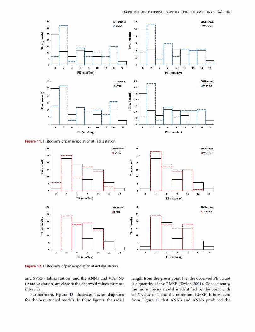
Probability distribution of the observed and predicteddata in the test period is presented in Figures 11 and12. These figures represent the probability occurrence ofa specific PE inside a particular interval (Al-Shammariet al., 2016). It can be comprehended that the proba-bility distributions of the predicted values of the ANN3

ENGINEERING APPLICATIONS OF COMPUTATIONAL FLUID MECHANICS 185

Figure 11. Histograms of pan evaporation at Tabriz station.

Figure 12. Histograms of pan evaporation at Antalya station.

and SVR3 (Tabriz station) and the ANN5 and WANN5(Antalya station) are close to the observed values formostintervals.

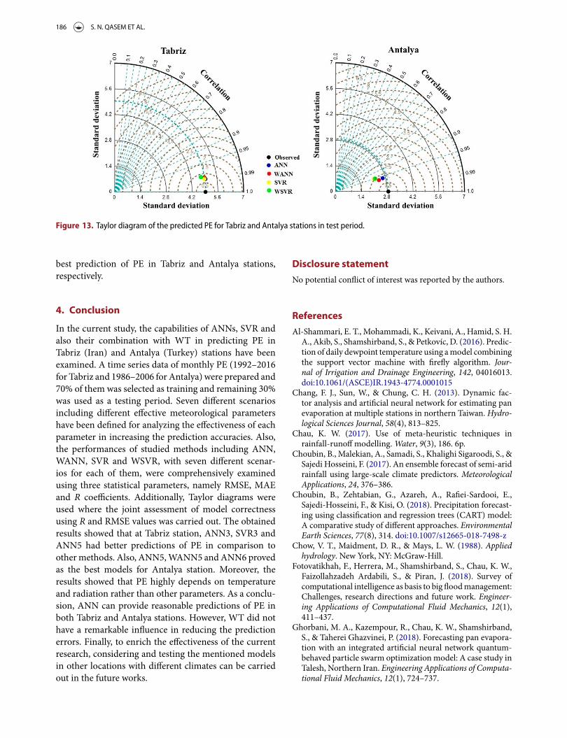
Furthermore, Figure 13 illustrates Taylor diagramsfor the best studied models. In these figures, the radial

length from the green point (i.e. the observed PE value)is a quantity of the RMSE (Taylor, 2001). Consequently,the more precise model is identified by the point withan R value of 1 and the minimum RMSE. It is evidentfrom Figure 13 that ANN3 and ANN5 produced the

186 S. N. QASEM ET AL.

Figure 13. Taylor diagram of the predicted PE for Tabriz and Antalya stations in test period.

best prediction of PE in Tabriz and Antalya stations,respectively.

4. Conclusion

In the current study, the capabilities of ANNs, SVR andalso their combination with WT in predicting PE inTabriz (Iran) and Antalya (Turkey) stations have beenexamined. A time series data of monthly PE (1992–2016for Tabriz and 1986–2006 for Antalya) were prepared and70% of them was selected as training and remaining 30%was used as a testing period. Seven different scenariosincluding different effective meteorological parametershave been defined for analyzing the effectiveness of eachparameter in increasing the prediction accuracies. Also,the performances of studied methods including ANN,WANN, SVR and WSVR, with seven different scenar-ios for each of them, were comprehensively examinedusing three statistical parameters, namely RMSE, MAEand R coefficients. Additionally, Taylor diagrams wereused where the joint assessment of model correctnessusing R and RMSE values was carried out. The obtainedresults showed that at Tabriz station, ANN3, SVR3 andANN5 had better predictions of PE in comparison toothermethods. Also, ANN5,WANN5 andANN6 provedas the best models for Antalya station. Moreover, theresults showed that PE highly depends on temperatureand radiation rather than other parameters. As a conclu-sion, ANN can provide reasonable predictions of PE inboth Tabriz and Antalya stations. However, WT did nothave a remarkable influence in reducing the predictionerrors. Finally, to enrich the effectiveness of the currentresearch, considering and testing the mentioned modelsin other locations with different climates can be carriedout in the future works.

Disclosure statement

No potential conflict of interest was reported by the authors.

References

Al-Shammari, E. T., Mohammadi, K., Keivani, A., Hamid, S. H.A., Akib, S., Shamshirband, S., & Petkovíc, D. (2016). Predic-tion of daily dewpoint temperature using amodel combiningthe support vector machine with firefly algorithm. Jour-nal of Irrigation and Drainage Engineering, 142, 04016013.doi:10.1061/(ASCE)IR.1943-4774.0001015

Chang, F. J., Sun, W., & Chung, C. H. (2013). Dynamic fac-tor analysis and artificial neural network for estimating panevaporation at multiple stations in northern Taiwan. Hydro-logical Sciences Journal, 58(4), 813–825.

Chau, K. W. (2017). Use of meta-heuristic techniques inrainfall-runoff modelling.Water, 9(3), 186. 6p.

Choubin, B., Malekian, A., Samadi, S., Khalighi Sigaroodi, S., &Sajedi Hosseini, F. (2017). An ensemble forecast of semi-aridrainfall using large-scale climate predictors. MeteorologicalApplications, 24, 376–386.

Choubin, B., Zehtabian, G., Azareh, A., Rafiei-Sardooi, E.,Sajedi-Hosseini, F., & Kisi, O. (2018). Precipitation forecast-ing using classification and regression trees (CART) model:A comparative study of different approaches. EnvironmentalEarth Sciences, 77(8), 314. doi:10.1007/s12665-018-7498-z

Chow, V. T., Maidment, D. R., & Mays, L. W. (1988). Appliedhydrology. New York, NY: McGraw-Hill.

Fotovatikhah, F., Herrera, M., Shamshirband, S., Chau, K. W.,Faizollahzadeh Ardabili, S., & Piran, J. (2018). Survey ofcomputational intelligence as basis to big floodmanagement:Challenges, research directions and future work. Engineer-ing Applications of Computational Fluid Mechanics, 12(1),411–437.

Ghorbani, M. A., Kazempour, R., Chau, K. W., Shamshirband,S., & Taherei Ghazvinei, P. (2018). Forecasting pan evapora-tion with an integrated artificial neural network quantum-behaved particle swarm optimization model: A case study inTalesh, Northern Iran. Engineering Applications of Computa-tional Fluid Mechanics, 12(1), 724–737.

ENGINEERING APPLICATIONS OF COMPUTATIONAL FLUID MECHANICS 187

Gleckler, P. J., Taylor, K. E., & Doutriaux, C. (2008). Perfor-mance metrics for climate models. Journal of GeophysicalResearch: Atmospheres, 113, D06104. doi:10.1029/2007JD008972

Goyal, M. K., Bharti, B., Quilty, J., Adamowski, J., & Pandey,A. (2014). Modelling of daily pan evaporation in sub trop-ical climates using ANN, LS-SVR, fuzzy logic, and ANFIS.Expert Systems with Applications, 41, 5267–5276.

Grossman, A., & Morlet, J. (1984). Decomposition of hardyfunctions into square integrable wavelets of constant shape.SIAM Journal on Mathematical Analysis, 15, 723–736.

Guven, A., & Kisi, O. (2013). Monthly pan evaporation mod-elling using linear genetic programming. Journal of Hydrol-ogy, 503, 178–185.

IPCC. (2007). Climate change 2007: The physical science basis.Intergovernmental Panel on Climate Change, 446, 727–728.

Jain, A., & Srinivasulu, S. (2004). Development of effectiveand efficient rainfall runoff models using integration ofdeterministic, real-coded genetic algorithms, and artificialneural network techniques. Water Resource Research, 40(4),W04302.

Keshtegar, B., Piri, J., & Kisi, O. (2016). A nonlinear mathemat-ical modeling of daily pan evaporation based on conjugategradient method. Computers and Electronics in Agriculture,127, 120–130.

Kim, S., & Kim, H. S. (2008). Neural networks and geneticalgorithm approach for nonlinear evaporation and evapo-transpirationmodelling. Journal of Hydrology, 351, 299–317.

Kisi, O. (2005). Suspended sediment estimation using neuro-fuzzy and neural network approaches. Hydrological SciencesJournal, 50(4), 683–696.

Kisi, O. (2006). Daily pan evaporationmodelling using a neuro-fuzzy computing technique. Journal of Hydrology, 329(3–4),636–646.

Kisi, O. (2009). Daily pan evaporation modelling using multi-layer perceptrons and radial basis neural networks. Hydro-logical Processed, 23, 213–223.

Kisi, O., Genc, O., Dinc, S., & Zounemat-Kermani, M. (2016).Daily pan evaporation modeling using chi-squared auto-matic interaction detector, neural networks, classificationand regression tree.Computers andElectronics inAgriculture,122, 112–117.

Kisi, O., & Tombul, M. (2013). Modelling monthly pan evapo-rations using fuzzy genetic approach. Journal of Hydrology,477, 203–212.

Lin, G. F., Lin, H. Y., & Wu, M. C. (2013). Development of asupport-vector-machine-basedmodel for daily pan evapora-tion estimation. Hydrological Processes, 27(22), 3115–3127.

McCulloch, W. S., & Pitts, W. H. (1943). A logical calculus ofthe ideas immanent in neural nets. Bulletin of MathematicalBiology, 5, 115–133.

Nourani, V., Alami, M. T., & Aminfar, M. (2009). A com-bined neural-wavelet model for prediction of Ligvanchaiwatershed precipitation. Engineering Applications of Artifi-cial Intelligence, 22(3), 466–472.

Nourani, V., Alami, M. T., & Daneshvar Vousoughi, F. (2015).Wavelet-entropy data pre-processing approach for ANN-based groundwater level modelling. Journal of Hydrology,524, 255–269.

Nourani, V., Hosseini Baghanam, A., Adamowski, J., & Kisi, O.(2014). Applications of hybrid wavelet-artificial Intelligence

models in hydrology: A review. Journal of Hydrology, 514,358–377.

Rajaee, T., Mirbagheri, S. A., Zounemat-Kermani, M., &Nourani, V. (2009). Daily suspended sediment concentrationsimulation using ANN and neuro-fuzzy models. Science ofthe Total Environment, 407, 4916–4927.

Rumelhart, D., & McClelland, J. (1986). Parallel distributedprocessing. Cambridge, MA: MIT Press.

Salas, J. D., Markus, M., & Tokar, A. S. (2000). Streamflow fore-casting based on artificial neural networks. In G. Rao &A. R.Rao (Eds.), Chapter 4 in artificial neural networks in hydrol-ogy (pp. 23–51). London: Kluwer Academic Publishers.

Samadianfard, S., Asadi, E., Jarhan, S., Kazemi, H., Khesht-gar, S., Kisi, O., . . . Abdul Manaf, A. (2018). Wavelet neuralnetworks and gene expression programming models to pre-dict short-term soil temperature at different depths. Soil andTillage Research, 175, 37–50.

Samadianfard, S., Delirhasannia, R., Kisi, O., &Agirre-Basurko,E. (2013). Comparative analysis of ozone level predictionmodels using gene expression programming and multiplelinear regression. GEOFIZIKA, 30, 43–74.

Samadianfard, S., Nazemi, A. H., & Sadraddini, A. A. (2014).M5 model tree and gene expression programming basedmodeling of sandy soil water movement under surfacedrip irrigation. Agriculture Science Developments, 3(5),178–190.

Samadianfard, S., Sattari, M. T., Kisi, O., & Kazemi, H. (2014).Determining flow friction factor in irrigation pipes usingdata mining and artificial intelligence approaches. AppliedArtificial Intelligence, 28, 793–813.

Shafaei, M., & Kisi, O. (2015). Lake level forecasting usingwavelet-SVR, wavelet-ANFIS and WaveletARMAconjunction models. Water Resource Management, 30(1),79–97.

Smola, A. J., & Scholkopf, B. (2004). A tutorial on supportvector regression. Statistics and Computing, 14(3), 199–222.

Stanhill, G. (2002). Is the Class A evaporation pan still the mostpractical and accurate meteorological method for determin-ing irrigation water requirements. Agricultural and ForestMeteorology, 112(3–4), 233–236.

Tabari, H., Marofi, S., & Sabziparvar, A. A. (2009). Estimationof daily pan evaporation using artificial neural network andmultivariate non-linear regression. Irrigation Science, 28(5),399–406.

Taormina, R., Chau, K. W., & Sivakumar, B. (2015). Neu-ral network river forecasting through baseflow separationand binary-coded swarmoptimization. Journal ofHydrology,529(3), 1788–1797.

Taylor, K. E. (2001). Summarizing multiple aspects of modelperformance in a single diagram. Journal of GeophysicalResearch: Atmospheres, 106, 7183–7192.

URL1. Retrieved from https://www.google.com/maps/@33.7728123,50.3526526,2214625 m/data= !3m1!1e3.

Vapnik, V. (1995). The nature of statistical learning theory. NewYork, NY: Springer Verlag.

Vapnik, V. (1998). Statistical learning theory. New York, NY:John Wiley & Sons.

Wang, W. C., Xu, D. M., Chau, K. W., & Chen, S. (2013).Improved annual rainfall-runoff forecasting using PSO-SVM model based on EEMD. Journal of Hydroinformatics,15(4), 1377–1390.