Embed Size (px)
Citation preview
Modeling Microbial Populations in the Chemostat
Hal Smith
A R I Z O N A S T A T E U N I V E R S I T Y
H.L. Smith (ASU) Modeling Microbial Populations in the Chemostat MBI, June 13, 2014 1 / 34

Outline
1 Why study microbial ecology?
2 Microbial GrowthGrowth under nutrient limitation, Monod(1942)
3 Continuous Culture: The ChemostatMicrobial Growth in the ChemostatCompetition for NutrientCompetitive Exclusion PrincipleThe Math supporting the CEP35 year old Open Problem
H.L. Smith (ASU) Modeling Microbial Populations in the Chemostat MBI, June 13, 2014 2 / 34

Why study microbial ecology?
Why study microbial ecology?
“The study of the growth of bacterial cultures does not constitute aspecialised subject or a branch of research: it is the basic method ofmicrobiology.” J. Monod, 1949
quantify microbial growth
quantify antibiotic efficacy
microbial ecology
bio-engineering: syntheticbio-fuels
waste treatment
bio-remediation
biofilms, quorum sensing
mammalian gut microflora
food, beverage (beer,wine)
H.L. Smith (ASU) Modeling Microbial Populations in the Chemostat MBI, June 13, 2014 3 / 34

Microbial Growth Growth under nutrient limitation, Monod(1942)
Growth rate and nutrient concentration
J. Monod, The growth of bacterial cultures, Annu. Rev. Microbiol. 1949
H.L. Smith (ASU) Modeling Microbial Populations in the Chemostat MBI, June 13, 2014 4 / 34

Microbial Growth Growth under nutrient limitation, Monod(1942)
Growth under Nutrient Limitation, Monod(1942)
Monod’s experimental data on bacterial growth rate as a function of nutrientconcentration led him to propose:
1 specific growth rate dNNdt varies with S = [glucose] approx. as
dNNdt
=rS
a + S
some r > 0 and a > 0.2 growth rate and nutrient consumption rate are proportional dN = γdS3 This implies that nutrient depletion is:
dSdt
= −1γ
rSNa + S
French biologist and nobelist Jacques Monod led an interesting life. Check it out on:http://en.wikipedia.org/wiki/Main_Page
H.L. Smith (ASU) Modeling Microbial Populations in the Chemostat MBI, June 13, 2014 5 / 34

Microbial Growth Growth under nutrient limitation, Monod(1942)
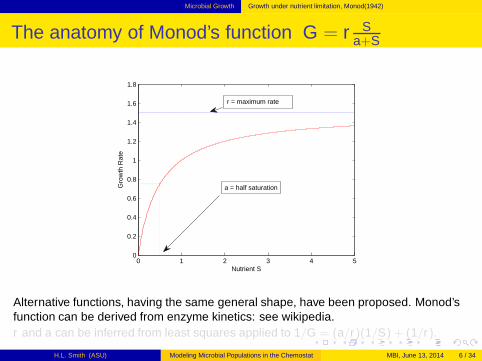
The anatomy of Monod’s function G = r Sa+S
0 1 2 3 4 50
0.2
0.4
0.6
0.8
1
1.2
1.4
1.6
1.8
Nutrient S
Gro
wth
Rat
e
r = maximum rate
a = half saturation
Alternative functions, having the same general shape, have been proposed. Monod’sfunction can be derived from enzyme kinetics: see wikipedia.r and a can be inferred from least squares applied to 1/G = (a/r)(1/S) + (1/r).
H.L. Smith (ASU) Modeling Microbial Populations in the Chemostat MBI, June 13, 2014 6 / 34
Microbial Growth Growth under nutrient limitation, Monod(1942)
The anatomy of Monod’s function G = r Sa+S
0 1 2 3 4 50
0.2
0.4
0.6
0.8
1
1.2
1.4
1.6
1.8
Nutrient S
Gro
wth
Rat
e
r = maximum rate
a = half saturation
Alternative functions, having the same general shape, have been proposed. Monod’sfunction can be derived from enzyme kinetics: see wikipedia.r and a can be inferred from least squares applied to 1/G = (a/r)(1/S) + (1/r).
H.L. Smith (ASU) Modeling Microbial Populations in the Chemostat MBI, June 13, 2014 6 / 34

Microbial Growth Growth under nutrient limitation, Monod(1942)
Growth in Batch Culture*
S-Nutrient.N-Bacteria.
dSdt
= −1γ
rSNa + S
dNdt
=rSN
a + S
0 1 2 3 4 5 6 70
0.5
1
1.5
2
2.5
time in hours
Batch Growth−−No maintenance
SN
*Batch culture is jargon for a closed-system culture, i.e., a covered Petri dish
H.L. Smith (ASU) Modeling Microbial Populations in the Chemostat MBI, June 13, 2014 7 / 34

Microbial Growth Growth under nutrient limitation, Monod(1942)
The principle of conservation of nutrient
dSdt
= −1γ
rSNa + S
dNdt
=rSN
a + S
Total nutrient, nutrient bound up in microbes plus free nutrient, is conserved:
ddt
(Nγ
+ S)
= 0 ⇒N(t)γ
+ S(t) =N(0)γ
+ S(0)
H.L. Smith (ASU) Modeling Microbial Populations in the Chemostat MBI, June 13, 2014 8 / 34

Continuous Culture: The Chemostat
The Chemostat: see Google images
H.L. Smith (ASU) Modeling Microbial Populations in the Chemostat MBI, June 13, 2014 9 / 34

Continuous Culture: The Chemostat
enter “Chemostat” into http://en.wikipedia.org/wiki/Main_Page
Substrate
Biomass V
DS D(S+x) 0
H.L. Smith (ASU) Modeling Microbial Populations in the Chemostat MBI, June 13, 2014 10 / 34

Continuous Culture: The Chemostat
The Old Tank Problem-No Bacteria
V = Volume of chemostat(ml)F = Inflow = Outflow rate (ml/hr)S0 = Concentration of Substrate in Feed (gm/ml).S = Concentration of Substrate in Chemostat (gm/ml).
Rate of change of Substrate (gm/hr)= INFLOW(gm/hr) - OUTFLOW(gm/hr)
ddt
(VS) = FS0 − FS
Let D = F/V be the Dilution Rate. Then
dSdt
= D(S0 − S)
Solution:S(t) = S(0)e−Dt + S0(1 − e−Dt ) → S0
H.L. Smith (ASU) Modeling Microbial Populations in the Chemostat MBI, June 13, 2014 11 / 34
Continuous Culture: The Chemostat Microbial Growth in the Chemostat
Classical Chemostat Model
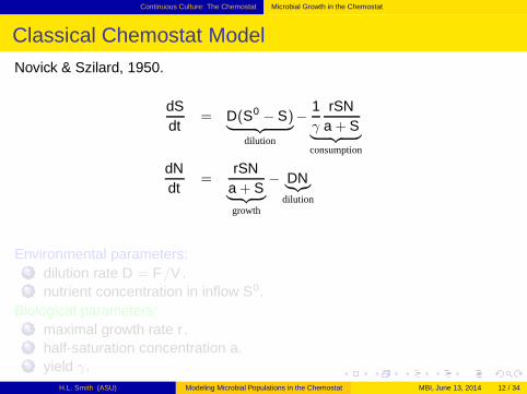
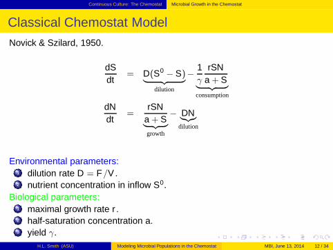
Novick & Szilard, 1950.
dSdt
= D(S0 − S)︸ ︷︷ ︸
dilution
−1γ
rSNa + S
︸ ︷︷ ︸
consumption
dNdt
=rSN
a + S︸ ︷︷ ︸
growth
− DN︸︷︷︸
dilution
Environmental parameters:1 dilution rate D = F/V .2 nutrient concentration in inflow S0.
Biological parameters:1 maximal growth rate r .2 half-saturation concentration a.3 yield γ.
H.L. Smith (ASU) Modeling Microbial Populations in the Chemostat MBI, June 13, 2014 12 / 34

Continuous Culture: The Chemostat Microbial Growth in the Chemostat
Classical Chemostat Model
Novick & Szilard, 1950.
dSdt
= D(S0 − S)︸ ︷︷ ︸
dilution
−1γ
rSNa + S
︸ ︷︷ ︸
consumption
dNdt
=rSN
a + S︸ ︷︷ ︸
growth
− DN︸︷︷︸
dilution
Environmental parameters:1 dilution rate D = F/V .2 nutrient concentration in inflow S0.
Biological parameters:1 maximal growth rate r .2 half-saturation concentration a.3 yield γ.
H.L. Smith (ASU) Modeling Microbial Populations in the Chemostat MBI, June 13, 2014 12 / 34

Continuous Culture: The Chemostat Microbial Growth in the Chemostat
Break-even nutrient level for survival of microbes
dNNdt
=rS
a + S− D = 0
when
S = λ =aD
r − D
0 1 2 3 4 50
0.2
0.4
0.6
0.8
1
1.2
1.4
1.6
1.8
Nutrient S
Gro
wth
Rat
e
D = Dilution rate
Break−even S
H.L. Smith (ASU) Modeling Microbial Populations in the Chemostat MBI, June 13, 2014 13 / 34

Continuous Culture: The Chemostat Microbial Growth in the Chemostat
Equilibria
0 = D(S0 − S)−1γ
rSNa + S
0 =
(rS
a + S− D
)
N
Washout Equilibrium: N = 0 and S = S0.
Survival Equilibrium: rSa+S = D, i.e., S = λ and N = γ(S0 − λ).
Positive survival equilibrium exists iff rS0
a+S0 > D.
H.L. Smith (ASU) Modeling Microbial Populations in the Chemostat MBI, June 13, 2014 14 / 34

Continuous Culture: The Chemostat Microbial Growth in the Chemostat
Phase Plane: Survival Equilibrium does not exist
S ’ = D (1 − S) − (2 S N)/(0.3 + S)N ’ = (2 S N)/(0.3 + S) − D N
D = 1.65
0 0.5 1 1.5
0
0.2
0.4
0.6
0.8
1
1.2
1.4
1.6
1.8
2
S
N
H.L. Smith (ASU) Modeling Microbial Populations in the Chemostat MBI, June 13, 2014 15 / 34

Continuous Culture: The Chemostat Microbial Growth in the Chemostat
Phase Plane: Survival Equilibrium exists
S ’ = D (1 − S) − (2 S N)/(0.3 + S)N ’ = (2 S N)/(0.3 + S) − D N
D = 1
0 0.5 1 1.5
0
0.2
0.4
0.6
0.8
1
1.2
1.4
1.6
1.8
2
S
N
H.L. Smith (ASU) Modeling Microbial Populations in the Chemostat MBI, June 13, 2014 16 / 34

Continuous Culture: The Chemostat Microbial Growth in the Chemostat
Stability of Washout Equilibrium
Small perturbations from the washout equilibrium obey the “linearizedsystem”:
(S,N) = (S0, 0) + (y1, y2), y = (y1, y2) small perturbation
y ′ = Jy
where J is the jacobian matrix at the washout equilibrium:
J =
(−D −f (S0)/γ0 f (S0)− D
)
The eigenvalues are −D and f (S0)− D, where f (S) = rSa+S .
The washout equilibrium is stable if rS0
a+S0 < D and unstable if rS0
a+S0 > D.
H.L. Smith (ASU) Modeling Microbial Populations in the Chemostat MBI, June 13, 2014 17 / 34

Continuous Culture: The Chemostat Microbial Growth in the Chemostat
Survival or Washout
If the inflow nutrient supply is sufficientfor the microbe to grow:
rS0
a + S0 > D,
then the bacteria survive:
N(t) → γ(S0 − λ), S(t) → λ,
Indeed, they are reproducing at theexponential rate set by dilution rate D.
Otherwise, they are washed out:
N(t) → 0, S(t) → S0
0 0.5 1 1.5 2 2.50
0.5
1
1.5
2
2.5
3
3.5
4
4.5
5
Survival
Extinction
D
S0
Operating Diagram
survival boundary: D = rS0
a+S0 .
H.L. Smith (ASU) Modeling Microbial Populations in the Chemostat MBI, June 13, 2014 18 / 34

Continuous Culture: The Chemostat Microbial Growth in the Chemostat
Phase Plane
S ’ = 1 − S − m S x/(a + S)x ’ = x (m S/(a + S) − 1)
m = 2a = 0.5
0 0.2 0.4 0.6 0.8 1 1.2 1.4 1.6 1.8 2
0
0.2
0.4
0.6
0.8
1
1.2
1.4
1.6
1.8
2
S
x
H.L. Smith (ASU) Modeling Microbial Populations in the Chemostat MBI, June 13, 2014 19 / 34

Continuous Culture: The Chemostat Microbial Growth in the Chemostat
The conservation principle
dSdt
= D(S0 − S)−1γ
rSNa + S
dNdt
=rSN
a + S− DN
Multiply N-eqn. by 1γ
and add to S eqn.:
ddt
[
S(t) +N(t)γ
]
= D(
S0 −
[
S(t) +N(t)γ
])
which implies that[
S(t) +N(t)γ
]
=
[
S(0) +N(0)γ
]
e−Dt + S0(1 − e−Dt)
Solution trajectory approaches line S + Nγ= S0.
H.L. Smith (ASU) Modeling Microbial Populations in the Chemostat MBI, June 13, 2014 20 / 34

Continuous Culture: The Chemostat Competition for Nutrient
Competing Strains of Bacteria
dSdt
= D(S0 − S)−1γ1
r1N1Sa1 + S
−1γ2
r2N2Sa2 + S
dN1
dt=
(r1S
a1 + S− D
)
N1
dN2
dt=
(r2S
a2 + S− D
)
N2
Exploitative Competition: each organism consumes a common resource.
H.L. Smith (ASU) Modeling Microbial Populations in the Chemostat MBI, June 13, 2014 21 / 34

Continuous Culture: The Chemostat Competition for Nutrient
Break-even concentrations
dN1
N1dt=
r1Sa1 + S
− D = 0 ⇔ S = λ1 =a1D
r1 − DdN2
N2dt=
r2Sa2 + S
− D = 0 ⇔ S = λ2 =a2D
r2 − D
0 1 2 3 4 50
0.2
0.4
0.6
0.8
1
1.2
1.4
1.6
1.8
Nutrient S
Gro
wth
Rat
e
Break−even values
lambda1
D
lambda2
λ1 = λ2? Coexistence at Equilibrium is Extremely Unlikely!H.L. Smith (ASU) Modeling Microbial Populations in the Chemostat MBI, June 13, 2014 22 / 34

Continuous Culture: The Chemostat Competition for Nutrient
No Coexistence Equilibria if λ1 6= λ2
N1 wins: S = λ1, N1 = γ1(S0 − λ1), N2 = 0
N2 wins: S = λ2, N1 = 0, N2 = γ2(S0 − λ2)
H.L. Smith (ASU) Modeling Microbial Populations in the Chemostat MBI, June 13, 2014 23 / 34

Continuous Culture: The Chemostat Competitive Exclusion Principle
Competitive Exclusion Principle: check it out on wikipedia
Assume each species can survive alone in the chemostat ( ri S0
ai+S0 > D.)
With no loss in generality, assume:
a1Dr1 − D
= λ1 < λ2 =a2D
r2 − D
Then N1 wins:
N1(t) → γ1(S0 − λ1), N2(t) → 0, S(t) → λ1
Winner is the organism that can grow at the lowest nutrient level.The winner of competition for nutrient is determined by quantities which maybe measured by growing each organism separately in the chemostat
Mathematical Proof: Hsu,Hubbell,Waltman (1977);Experimental Test: Hansen & Hubbell (1980)
H.L. Smith (ASU) Modeling Microbial Populations in the Chemostat MBI, June 13, 2014 24 / 34

Continuous Culture: The Chemostat The Math supporting the CEP
Conservation Principle
ddt
[
S(t) +N1(t)γ1
+N2(t)γ2
]
= D(
S0 −
[
S(t) +N(t1)γ1
+N2(t)γ2
])
which implies that
S(t) +N1(t)γ1
+N2(t)γ2
→ S0.
This suggests setting S(t) + N1(t)γ1
+ N2(t)γ2
= S0 and xi =Ni (t)γi
:
dx1
dt=
(f1(S0 − x1(t) − x2(t)) − D
)x1
dx2
dt=
(f2(S0 − x1(t) − x2(t)) − D
)x2
where
fi(S) =riS
ai + S
H.L. Smith (ASU) Modeling Microbial Populations in the Chemostat MBI, June 13, 2014 25 / 34

Continuous Culture: The Chemostat The Math supporting the CEP
Stability of Equilibria: 0 < λ1 < λ2 < S0
The Jacobian Matrix evaluated at the non-zero equilibria.
At x̂1 = S0 − λ1, x̂2 = 0
J =
(−x̂1f ′1 −x̂1f ′1
0 f2(λ1)− D
)
f2(λ1)− D < f2(λ2)− D = 0 sodiagonal entries are negative.Asymptotically Stable.
At x̃1 = 0, x̃2 = S0 − λ2
Jacobian =
(f1(λ2)− D 0
−x̃2f ′2 −x̃2f ′2
)
f1(λ2)− D > f1(λ1)− D = 0 so redentry is positive. Unstable Saddle.
H.L. Smith (ASU) Modeling Microbial Populations in the Chemostat MBI, June 13, 2014 26 / 34

Continuous Culture: The Chemostat The Math supporting the CEP
No Periodic Orbits
Dulac’s Criterion satisfied:
∂
∂x1
(f1 − D)x1
x1x2+
∂
∂x2
(f2 − D)x1
x1x2= −
(f ′1x2
+f ′2x1
)
< 0
Learn about Dulac’s Criterion at:
http://www.scholarpedia.org/article/Encyclopedia_of_dynamical_systems
H.L. Smith (ASU) Modeling Microbial Populations in the Chemostat MBI, June 13, 2014 27 / 34

Continuous Culture: The Chemostat The Math supporting the CEP
The Phase Plane of Competition
x1 ’ = 1.2 x1 (1 − x1 − x2)/(1.01 − x1 − x2) − x1x2 ’ = 1.5 x2 (1 − x1 − x2)/(1.1 − x1 − x2) − x2
0 0.1 0.2 0.3 0.4 0.5 0.6 0.7 0.8 0.9 1
0
0.1
0.2
0.3
0.4
0.5
0.6
0.7
0.8
0.9
1
x1
x2
H.L. Smith (ASU) Modeling Microbial Populations in the Chemostat MBI, June 13, 2014 28 / 34

Continuous Culture: The Chemostat The Math supporting the CEP
Winner may depend on dilution rate
0 1 2 3 4 50
0.2
0.4
0.6
0.8
1
1.2
1.4
1.6
1.8
Nutrient S
Gro
wth
Rat
e
Break−even values
lambda1
D
lambda2
λ2 < λ1 so N2 wins.By increasing D a bit, green line goes up, so λ1 < λ2 and N1 wins!
H.L. Smith (ASU) Modeling Microbial Populations in the Chemostat MBI, June 13, 2014 29 / 34

Continuous Culture: The Chemostat The Math supporting the CEP
Species 1 Wins when D = 1.16
x ’ = 1.2 x (1 − x − y)/(1.01 − x − y) − D xy ’ = 1.5 y (1 − x − y)/(1.1 − x − y) − D y
D = 1.16
0 0.1 0.2 0.3 0.4 0.5 0.6 0.7 0.8 0.9 1
0
0.1
0.2
0.3
0.4
0.5
0.6
0.7
0.8
0.9
1
x
y
H.L. Smith (ASU) Modeling Microbial Populations in the Chemostat MBI, June 13, 2014 30 / 34

Continuous Culture: The Chemostat The Math supporting the CEP
Species 2 Wins when D = 1.17
x ’ = 1.2 x (1 − x − y)/(1.01 − x − y) − D xy ’ = 1.5 y (1 − x − y)/(1.1 − x − y) − D y
D = 1.17
0 0.1 0.2 0.3 0.4 0.5 0.6 0.7 0.8 0.9 1
0
0.1
0.2
0.3
0.4
0.5
0.6
0.7
0.8
0.9
1
x
y
H.L. Smith (ASU) Modeling Microbial Populations in the Chemostat MBI, June 13, 2014 31 / 34
Continuous Culture: The Chemostat 35 year old Open Problem
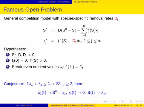
Famous Open Problem
General competition model with species-specific removal rates Dj
S′ = D(S0 − S)−n∑
j=1
fj(S)xj
x ′
j = (fj (S)− Dj)xj , 1 ≤ j ≤ n.
Hypotheses:1 S0,D,Dj > 0.2 fj(0) = 0, f ′j (S) > 0.3 Break-even nutrient values λj : fj (λj) = Dj .
Conjecture: If λ1 < λ2 ≤ λj < S0, j ≥ 2, then:
x1(t) → S0 − λ1, xj(t) → 0, S(t) → λ1.
H.L. Smith (ASU) Modeling Microbial Populations in the Chemostat MBI, June 13, 2014 32 / 34

Continuous Culture: The Chemostat 35 year old Open Problem
Proofs of the Competitive Exclusion Principle.
Author(s) and Date HypothesesHsu, Hubbel, Waltman 1977 D = Di and fi MonodHsu 1978 fi MonodArmstrong & McGehee 1980 Di = D, fi monotoneButler & Wolkowicz 1985 Di = D, fi mixed-monotoneWolkowicz & Lu 1992 Di 6= D, fi mixed-monotone, add. assumptionsWolkowicz & Xia 1997 Di − D small, fi monotoneLi 1998,1999 Di − D small, fi mixed-monotoneLiu et al 2013 allows time delays for nutrient assimilationYour Name, Date Di 6= D, fi monotone
mixed-monotone means one-humped.
H.L. Smith (ASU) Modeling Microbial Populations in the Chemostat MBI, June 13, 2014 33 / 34

Continuous Culture: The Chemostat 35 year old Open Problem
References
The Theory of the Chemostat, Smith and Waltman, Cambridge Studies inMathematical Biology, 1995Microbial Growth Kinetics, N. Panikov, Chapman& Hall, 1995Resource Competition, J. Grover, Chapman& Hall, 1997
H.L. Smith (ASU) Modeling Microbial Populations in the Chemostat MBI, June 13, 2014 34 / 34