Embed Size (px)
Citation preview

Modeling interferometers with lensdesign software
Bryan D. Stone, MEMBER SPIETropel Corporation60 O’Connor RoadFairport, New York 14450
Abstract. Lens design software has been designed primarily to modelconventional imaging systems. While interferometers do not generallyfall into this category, lens design software nonetheless is well suited foranalyzing a variety of aspects of interferometric systems. The generalrequirements for a ray-based model of interferometers are discussed,and a variety of examples are presented. The examples are designed todemonstrate both the power and flexibility of the approach proposedhere for modeling interferometers. © 2000 Society of Photo-Optical Instrumenta-tion Engineers. [S0091-3286(00)01307-6]
Subject terms: lens design; interferometers; imaging systems.
Paper ENV-13 received Oct. 26, 1999; revised manuscript received Feb. 7, 2000;accepted for publication Feb. 7, 2000.
sigw-
inge otheit.
tingdetemaceexite-the
re,irdee-p-ute-
lsreisnve
lge-
r-sknd
ng
s-emarete
in-ys
ti-pa-s-
gh
oth;re-rate
ofts,
canx-ot
se,er-
delhisrilyichc. 3re-od-olics insionx-
er-ea-
on
1 Introduction
Geometrical optics has been used successfully to deconventional imaging systems for hundreds of years. Hoever, simple spot diagrams are insufficient for modelsystems whose aberrations are small—the wave naturlight must be taken into account to accurately predictbehavior of systems as they approach the diffraction limA simple ray-based analysis does a good job of predicthe shape of wavefronts away from caustics, but the mobreaks down near caustics. Since in an imaging systhere is a caustic at the image plane, it is common to trrays only to estimate the shape of the wavefront in thepupil. If quantities like the point spread function are dsired, this wavefront is then propagated according tolaws of wave optics to the image plane.
Contrast this with interferometers. By their very natuthey rely explicitly on the wave nature of light for theoperation. However, in interferometers, caustics at thetector are typically avoided. Therefore, for any given wavfront that is input into the interferometer, geometrical otics generally does a good job of predicting the outpwavefront. And it is the path difference between wavfronts that interferometers measure.
Despite the obvious utility of the relatively simple tooof geometrical optics for modeling interferometers, theare studies in which the propagation of fieldsconsidered.1,2 However, the bulk of the published work omodeling interferometers centers on the geometric wafront. Huang discusses propagation errors within an abraic framework for Fizeau interferometry.3 A number ofpapers describing numerical modeling of individual inteferometers have been published. For example, Michaloet al. develop a method for modeling interferometers aapply it to a grazing-incidence interferometer for testicylindrical parts.4 Lowman and Greivenkamp5,6 consider aTwyman-Green interferometer for nonnull testing of apheres. In another paper, misalignments of optical assblies in an interferometer for astrometric measurementstudied.7 All of these papers use ray tracing to estima
1748 Opt. Eng. 39(7) 1748–1759 (July 2000) 0091-3286/2000/$15
Downloaded from SPIE Digital Library on 06 Jan 201
n
f
l
-
-
i
-
geometric wavefronts. An alternative approach thatvolves tracing a large number of randomly chosen rathrough an interferometer has also been described.8
A general, geometric framework for modeling the opcal performance of interferometers is described in thisper. This framework allows for modeling a variety of apects of interferometers. These include~but are not limitedto! ~i! the sensitivity of an interferometer to manufacturinerrors in its components;~ii ! the effects associated witaberrated input wavefronts;~iii ! the reduction in visibilitydue to an extended source, a polychromatic source, or b~iv! determining the range of amplitudes and spatial fquencies over which an interferometer can make accumeasurements. This framework is applied to the testingoptical surfaces~interferometers that measure rough parfor example, are not modeled well with this approach* !.Note that not all aspects of interferometer performancebe modeled with this simple geometric framework. For eample, if the viewing optics in an interferometer do nimage a part under test, say, onto the detector, thendefocusfringes are observed at the edge of the part. In this cadiffraction effects must be considered to predict the intference pattern seen at the detector.
The basic premise for the proposed approach is to mointerferometers in the manner in which they are used. Tis discussed further in Sec. 2. Sections 3, 4, and 5 primaconsist of a variety of examples showing the ways in whthis basic approach can be applied. The example of Seinvolves a Twyman-Green interferometer. The measument error associated with an aberrated input beam is meled, and a simulation of the measurement of a parabsurface is described. This same interferometer appearexamples presented in Sec. 4 and 5. In Sec. 4, a discusof modeling extended sources is given, along with eamples for a Michelson and for the Twyman-Green intferometer. In Sec. 5, a method to map out the useful m
*Rough partsare those with features on the surface with dimensionsthe order of the wavelength.
.00 © 2000 Society of Photo-Optical Instrumentation Engineers
2 to 199.197.130.217. Terms of Use: http://spiedl.org/terms

atier,m-ror.avedeitteridesth-needth
inger.y ar isandthe
ar
t
er-
twe.lutethe
ter’there-un
re isable
ve-tor.eoft-y,h alandare
aretheiononeial.hednt.ontsndas
re,se-
ingw-re,c-er-the
ora
be
Bryan D. Stone: Modeling interferometers with lens design software
surement range of an interferometer is described@thiscovers item~iv! in the above list#. Concluding remarks areoffered in Sec. 6.
2 Basic Approach
2.1 General Description
Consider the Tyman-Green interferometer shown schemcally in Fig. 1. An input beam is incident on a beamsplittwhich sends the light into the two arms of the interferoeter. The reference arm is shown with a plane return mirThe test arm has a feed lens to generate spherical wfronts. The detector is placed conjugate to the part untest~viewing optics can be added between the beamspland the detector to image the test part onto the detecto!. Ifa plane wave enters the system and all elements are~both in design and manufacture!, then a plane wave exiteach arm of the interferometer. In practice, however, noing is perfect, and there are a variety of effects that omight want to model: aberrated input wavefronts, extendsources, polychromatic sources, aberrations inherent indesign of the feed or viewing optics, and manufacturerrors or misalignments of elements in the interferomet
By developing an approach that matches, as closelpossible, the conditions under which the interferometeused, it is possible to model all these effects. To understthis approach, consider Fig. 2, where the two arms ofinterferometer are shown separately. A wavefront~not nec-essarily plane! is input into the system, and a particulpoint on the detector is labeledA. Now consider a raythrough the test arm that~i! is normal to the wavefront and~ii ! passes through the pointA on the detector. This rayintersects the wavefront at the point labeledB. A similarray through the reference arm~that passes throughA and isnormal to the input wavefront! also is shown. The poinwhere this ray intersects the wavefront is labeledC. At thepoint A, the interferometer measures the optical path diffence ~OPD! between the raysBA and CA. The OPD isobtained by measuring the relative phase between theinterfering wavefronts atA and then unwrapping that phasThere are a variety of methods for measuring absophase and performing the phase unwrapping. Whilechoices made for these methods affect the interferomeperformance, the focus of this paper is on modelingeffects of the optics on interferometer performance. Thefore, the assumption is made that phase detection andwrapping are performed perfectly.
Based on the above discussion, if lens design softwaused to model the interferometer, the software must be
Fig. 1 A schematic of a simple Twyman-Green interferometer.
Downloaded from SPIE Digital Library on 06 Jan 201
-
-rr
al
e
s
o
s
-
to determine the ray that is normal to any given input wafront and passes through any given point on the detecThis process I callray aiming, because it is related to thray aiming that commonly takes place in lens design sware when determining the initial direction of a ray, sathat starts at a given object point and passes througgiven point in the exit pupil. Proper ray aiming is criticafor the ultimate success of the approach taken here,some considerations for performing such ray aimingdiscussed in the next subsection.
Before presenting that discussion, a few thoughtsgiven on the advantages of this procedure. Since it isinterference between wavefronts that gives informatabout the OPD between arms of an interferometer,could argue that the step of ray aiming is not essentInstead, rays normal to the input wavefront can be launcfrom, say, points on a regular grid across the wavefroOnce these rays are traced to the detector, the wavefrfor the different arms of the interferometer can be fitted athen subtracted. However, this procedure is not alwaysclean as it sounds. Some of the issues~which are discussedfirst! relate to the operation of current lens design softwabut others are more fundamental. If one wants to ubuilt-in features of lens design software, this typically limits the input wavefronts to planes and spheres. In fittwavefronts, Zernike polynomials are typically used. Hoever, if the part does not have a circular clear apertuZernike polynomials are not the best choice of fitting funtions: a set of functions that are orthogonal over the apture shape is required. Further, mapping errors betweenwavefronts from different arms have to be allowed fseparately. In general, fitting the output wavefronts isprocess fraught with pitfalls, and the user must alwayson the lookout for poor fits.
Fig. 2 (a) The test arm and (b) the reference arm in a Twyman-Green interferometer. A ray through each arm of the interferometeris shown that (i) passes through a given point on the detector (la-beled A) and (ii) is normal to the input wavefront.
1749Optical Engineering, Vol. 39 No. 7, July 2000
2 to 199.197.130.217. Terms of Use: http://spiedl.org/terms

ereor
n tothe
iseri
gh-e iedhetedursthe
l ofoc-ysthethe
thoc-
hatw.
ally
ventheThor
ngnyinghisle-gh
ay-rgereforth
ysnti-arare-oormi-
st
ay
me
at
ednt,
itiononntn-
re-
thei-
odtep
anbeifiedr9.utingofthe, athe
istendof
ialofr
aveat
tous-nttestnce
Thispre-in
mmnter
ven-nedr is
Bryan D. Stone: Modeling interferometers with lens design software
The problems listed above could be considered minconveniences—they can all be overcome in one wayanother. However, there is a more fundamental reasoavoid the above procedure: when modeling the limits toperformance of an interferometer~as is done in Sec. 5!,fitting is inadequate. For example, the ray aiming thatused here sometimes fails. This can occur for large asphdepartures with a nonnull test, for example, or when hispatial-frequency errors are placed on parts, as is donSec. 5. However, if a robust ray-aiming procedure is usthese failures provide useful information. Failures of tray-aiming algorithm signal that a caustic of the associawavefront has moved onto the detector. When this occthe measurement that is made is not simply related tosurface figure of the part under test. Any robust modeinterferometer performance should be vigilant for suchcurrences and alert the user to them. If a grid of rathrough the input wavefront is sent into the system andoptical path of the output rays is used to fit a wavefront,result is meaningless once a caustic has moved ontodetector. However, one might never know that this hascurred.
The only drawback of the method proposed here is tit is iterative, and therefore has the potential to be sloHowever, such an iterative procedure is not fundamentdifferent ~and no more costly! from determining the initialdirection of a ray on the object that passes through a gipoint on the exit pupil. Computers are fast, and tracingextra rays is generally of little consequence these days.advantage is that this method provides a general framewfor analyzing a variety of interferometers. By incorporatithe ray aiming with conventional lens design software, acomponent that can be included in a conventional imagsystem can be included in an interferometer model. Tincludes gratings, diffractive elements, gradient-index ements, aspheres, etc. In the next subsection, some thouon ray aiming are given.
2.2 Considerations for Ray Aiming
There are two properties that are important for any raiming procedure: it must be robust, and it must convequickly. In assessing the tradeoffs between these twoquirements, it is generally desirable to sacrifice speedthe sake of robustness. For quick convergence, I useNewton-Raphson method~see, e.g., Ref. 9!, which is de-scribed briefly as follows. Place a Cartesian coordinate stem at the detector and one at the input wavefront. Quaties associated with the detector’s coordinate systemdistinguished by the addition of a prime, and the axeschosen such that theX8 andY8 coordinates of a point correspond to transverse positions on the detector. The cdinate system associated with the input wavefront is silarly aligned so that theX and Y coordinates uniquelyidentify a point on the wavefront. Given a point of intereon the detector with coordinates (x8,y8), the goal is todetermine the position on the input wavefront for the rthat ~i! starts normal to the wavefront and~ii ! passesthrough the point of interest on the detector. Given soguess for this initial position@call the coordinates of thisguess (x0 ,y0)#, the coordinates of the ray from this pointthe detector can be determined@call them (x08 ,y08)#. Then
1750 Optical Engineering, Vol. 39 No. 7, July 2000
Downloaded from SPIE Digital Library on 06 Jan 201
c
n,
,
e
ek
ts
-
e
-
e
-
according to the Newton-Raphson method, an ‘‘improvestimate’’ for the desired position on the input wavefro(x1 ,y1) say, is given by
S x1
y1D5S x0
y0D1F ]x08/]x0 ]x08/]y0
]y08/]x0 ]y08/]y0G21S x82x08
y82y08D , ~1!
where the derivatives represent the changes in ray posat the detector with respect to changes in ray positionthe wavefront.~These derivatives must take into accouthe change in initial ray direction for non-plane-wave iputs.!
This method, on its own, fails the robustness requiment~see, e.g., Ref. 10!. If, for example, the initial guess isnot close enough to the actual point on the wavefront,‘‘improved estimate’’ may actually be worse than the orignal estimate. To allow for such a possibility, the methcan be supplemented with a check of whether the sspecified by Eq.~1! ~in the second term on the right! givesa point further from the desired point on the detector ththe initial guess did. If it does, a smaller step cansearched for that gives an output ray closer to the specpoint on the detector.~The method I use for this is similato the one described in Sec. 9.7 of the book cited in Ref.!
Another way this method can fail is that the outppoints can oscillate around the desired point, convergonly slowly. To fix this problem, an estimate of the rateconvergence can be determined from one iteration tonext. If the convergence after a few iterations is too slowsmaller step that gives an output ray that is closer tospecified point on the detector can be searched for.
Finally, a means to determine the initial estimateneeded. Since the coordinates of points at the detectorto be approximately linearly related to the coordinatespoints at the input, taking the initial ray to start at the axpoint on the wavefront works well. However, in casesunconventional geometries,† more specialized methods fofinding initial estimates may be needed.
The process described above is very robust, and I hfound that it fails only in cases where there is a causticthe detector.
3 A Basic Twyman-Green Interferometer
3.1 Example 1: Measuring a Sphere
For this example, a Twyman-Green interferometer usedtest a spherical part is modeled. The interferometer is illtrated schematically in Fig. 3. The input beam is incideon a cube beamsplitter. A feed lens and the part underconstitute the test arm, and a plane mirror the referearm. Viewing optics~in the form of an afocal pair! havebeen placed between the beamsplitter and the detector.pair images the part under test onto the detector. Thescriptions for the feed lens and viewing optics are givenan appendix. The part under test is taken to have a 100-radius of curvature and a 50-mm clear aperture. The ce
†An embodiment of an interferometer that I consider possesses uncontional geometry is the CylinderMaster™. This interferometer is desigto measure cylindrical parts at near-grazing incidence. CylinderMastea trademark of Tropel Corporation, Fairport, NY.
2 to 199.197.130.217. Terms of Use: http://spiedl.org/terms

ofheleeen
eNe
f aallyFo
or
erstw
OPeroPD
ted
ri-t ththedePD
t isemhee togli-
heayof
icalr
d theat
urethe
has
theub-
themmtheentled
ure-usthethebether
Bryan D. Stone: Modeling interferometers with lens design software
of curvature of the part is placed at the rear focal pointthe feed lens.~The separation from the last surface of tfeed to the rear focal point is given in the last row of Tab1 in the appendix.! The input beam diameter that fills thclear aperture of the part is 4.0 mm. The measuremwavelength in all examples presented here is that of a Hlaser~0.6328mm!.
For the first example, consider the measurement operfect spherical part. The points of interest are equspaced along a line through the center of the detector.each point, the initial position of two rays~one through thetest arm and the other through the reference! are deter-mined. These rays~i! pass through the point on the detectand ~ii ! are normal to the~in this case plane! input wave-front. Note that because of the nature of interferometany constant can be added to the OPD between thearms. This constant is chosen such that the measuredbetween the rays at the center of the part under test is zThe resultant OPD is plotted in Fig. 4. The measured Ois simply twice the wavefront error of the feed lens~twicebecause the feed lens is double-passed!. When high accu-racy is desired, the OPD shown in Fig. 4 can be subtracfrom any measurements~i.e., it can be calibrated out!.
Now consider adding half a wave of third-order sphecal aberration to the input beam. The measurement thainterferometer gives for various separations betweenbeamsplitter cube endface and the reference mirror istermined according to the model, and the measured O
Fig. 3 Illustration of the Twyman-Green interferometer appearing inexamples in Secs. 3, 4, and 5.
Fig. 4 Measured OPD (in waves) as a function of position on thepart for the Twyman-Green interferometer illustrated in Fig. 3.
Downloaded from SPIE Digital Library on 06 Jan 201
t
r
,oD.
e
-
for a plane wave input is subtracted from this. The resulplotted in Fig. 5 for five different locations of the referencmirror. When the reference mirror is placed 43.81 mm frothe beamsplitter, it is imaged by the viewing optics onto tdetector. Since the surface under test is also conjugatthe detector, the effect of an aberrated input beam is negible for this position of the reference mirror. However, tpropagation effects as the reference mirror is moved awfrom this position become noticeable. At a distance163.25 mm, the two arms have approximately equal optpaths along the axis~this condition needs to be satisfied, foexample, when a temporally incoherent source is used!. Inthis case, the difference between the measured OPD anOPD found with a plane-wave input is about 0.05 wavesthe edge of the part.
3.2 Example 2: Measuring a Paraboloid
The Twyman-Green interferometer is now used to measa paraboloid with the same base radius of curvature assphere from the previous subsection.@A paraboloid with aclear aperture of 50 mm and a base radius of 100 mmabout 0.05 mm~or 80 waves at HeNe! of departure fromthe sphere with the same base radius.# The input wavefrontis taken to be plane. In this case, I focus solely onpropagation errors in the system, and therefore again stract the OPD due to the feed lens from the OPD ofmeasurement. Say the part is positioned precisely 100from the focus of the feed. Then as one moves out onpart, the test gets further from null, and the measuremerror increases. This is shown in Fig. 6 as the curve labe0.0 mm. The other curves in Fig. 6 represent the measment error as the part is shifted axially away from the focof the feed lens. The label of each curve shows how farbase center of curvature of the part has moved fromfocus of the feed lens. When the part is shifted, it canmeasured well in two zones: one near the axis and ano
Fig. 5 This figure shows the change in measured OPD when theinput beam possesses 0.5 waves of third-order spherical aberration.The different curves are for different positions of the reference mir-ror.
1751Optical Engineering, Vol. 39 No. 7, July 2000
2 to 199.197.130.217. Terms of Use: http://spiedl.org/terms

omt onedanditch
c-
el-rceanretnedi-is-
si-an
,
rgy
itsees
cya
-del
e
he
sed to
Bryan D. Stone: Modeling interferometers with lens design software
near a null of constant radius. As the part moves away frthe feed, the radius of the second null zone moves outhe part, and the regions~both near the axis and in thsecond null zone! over which the interferometer gives goodata get narrower. This model can determine the sizenumber of zones required for accurate subaperture sting. Of course, the fringe densities~which get higher awayfrom the null! also have to be taken into account for detetors with discrete pixels.
4 Extended Sources
4.1 Discussion
The approach taken here allows for straightforward moding of the effects of extended sources. Extended soutend to decrease fringe visibility. To model this effect,extended source is approximated by a series of discsources that add incoherently. Each discrete source geates an independent input wavefront. Consider the irraanceI at a point on the detector resulting from these dcrete wavefronts. In a two-beam interferometer~such as aFizeau or Twyman-Green!, the irradiance is given by
I ~wz!5(i 51
N
wiF11v i cosS 2p
ld i1wzD G , ~2!
whereN is the number of discrete sources,d i is the OPD~associated with the point on the detector! for wavefronti,v i is the visibility associated with sourcei alone,wi is aweighting for the different input wavefronts, andwz is aphase term. Aswz is varied from 0 to 2p, the irradiancegoes through its maximum and minimum values. Phycally, this phase shift can be thought of as resulting fromaxial shift of a reference mirror~in a Twyman-Green inter-ferometer, say! or of the part~in a Fizeau interferometersay!. Eachv i must be between zero and one~thev i are lessthan unity, for example, when different amounts of eneexit the source and reference arms!.
Fig. 6 A logarithmic plot of the measurement error as a function ofradial position on the part under test. The different curves are forvarious positions of the part. The label associated with each curveshows the amount the center of curvature of the part is shifted fromthe focus of the feed lens.
1752 Optical Engineering, Vol. 39 No. 7, July 2000
Downloaded from SPIE Digital Library on 06 Jan 201
-
s
er-
As an aside, there are a variety of reasons for thewi notto be equal. For example, thewi can be adjusted for anuneven energy distribution across the source~so that eachinput wavefront gets a different weighting according toenergy!. As another example, Eq.~2! represents a discretapproximation to a continuous integral. Different schemfor numerical integration, such as Gaussian quadrature,‡ re-quire different weightings to achieve the highest accurafrom the numerical approximation. Therefore, even foruniform source, thewi are not necessarily equal.
Equation~2! is now put into a form that makes it obvious how the framework introduced earlier is used to moextended sources. Begin by rewriting it as
I ~wz!5(i 51
N
wi1coswz F(i 51
N
wiv i cosS 2p
ld i D G
2sinwz F(i 51
N
wiv i sinS 2p
ld i D G . ~3!
The visibility ~denoted byV! is defined as
V5I max2I min
I max1I min, ~4!
where I max is the maximum value of the irradiance aswz
varies, andI min the minimum value. Letwz,max and wz,min
be the values ofwz that maximize and minimizeI, respec-tively. These are found by differentiating Eq.~3! with re-spect towz and setting the result equal to zero:
wz,max5tan21F (i 51
N
wiv i sinS 2p
ld i D
(i 51
N
wiv i cosS 2p
ld i D G , ~5!
wz,min5wz,min1p. ~6!
Equations~3!, ~4!, ~5!, and~6! can be combined to give thfollowing expression for the visibility:
V5
H F(i 51
N
wiv i sinS 2p
ld i D G 2
1F(i 51
N
wiv i cosS 2p
ld i D G 2J 1/2
(i 51
N
wiv i
.~7!
While Eq. ~7! can be manipulated further,§ this form isideal for numerical implementation. For each point on tsource~i.e., for each input wavefront!, the OPD between
‡For example, the quadrature schemes discussed in Ref. 11 can be uobtain the most accuracy with the fewest input wavefronts.
§For example, Eq.~7! is equivalent to the following equation:
V5
HF(i51
N
~wivi!2G12(
i51
N
(j5i11
N
wiwjvivj cosF2p
l~di2dj!GJ1/2
(i51
N
wivi
.
2 to 199.197.130.217. Terms of Use: http://spiedl.org/terms
p-t isq.
Asrepleatwoour7.
fors
rare
theaide
-
th
Inf
at
al-
ical
toThetheedaical-als
sts,xact
thekeen
g
Bryan D. Stone: Modeling interferometers with lens design software
the arms of the interferometer is determined~i.e., thed i arefound!. Running totals are kept of the individual sums apearing in Eq.~7!. Once the sums have been computed, istraightforward to determine the visibility according to E~7!.
4.2 Example 1: Michelson Interferometer
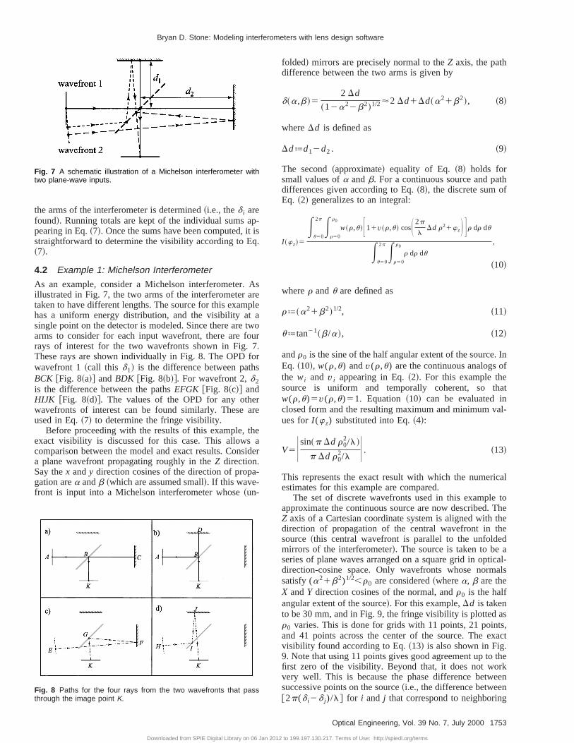
As an example, consider a Michelson interferometer.illustrated in Fig. 7, the two arms of the interferometer ataken to have different lengths. The source for this examhas a uniform energy distribution, and the visibility atsingle point on the detector is modeled. Since there arearms to consider for each input wavefront, there are frays of interest for the two wavefronts shown in Fig.These rays are shown individually in Fig. 8. The OPDwavefront 1~call this d1! is the difference between pathBCK @Fig. 8~a!# andBDK @Fig. 8~b!#. For wavefront 2,d2is the difference between the pathsEFGK @Fig. 8~c!# andHIJK @Fig. 8~d!#. The values of the OPD for any othewavefronts of interest can be found similarly. Theseused in Eq.~7! to determine the fringe visibility.
Before proceeding with the results of this example,exact visibility is discussed for this case. This allowscomparison between the model and exact results. Consa plane wavefront propagating roughly in theZ direction.Say thex andy direction cosines of the direction of propagation area andb ~which are assumed small!. If this wave-front is input into a Michelson interferometer whose~un-
Fig. 7 A schematic illustration of a Michelson interferometer withtwo plane-wave inputs.
Fig. 8 Paths for the four rays from the two wavefronts that passthrough the image point K.
Downloaded from SPIE Digital Library on 06 Jan 201
r
folded! mirrors are precisely normal to theZ axis, the pathdifference between the two arms is given by
d~a,b!52 Dd
~12a22b2!1/2'2 Dd1Dd~a21b2!, ~8!
whereDd is defined as
Ddªd12d2 . ~9!
The second~approximate! equality of Eq. ~8! holds forsmall values ofa andb. For a continuous source and padifferences given according to Eq.~8!, the discrete sum ofEq. ~2! generalizes to an integral:
I ~wz!5
Eu50
2p Er50
r0
w~r,u!F11v~r,u! cosS 2p
lDd r21wzD Gr dr du
Eu50
2p Er50
r0
r dr du
,
~10!
wherer andu are defined as
rª~a21b2!1/2, ~11!
uªtan21~b/a!, ~12!
andr0 is the sine of the half angular extent of the source.Eq. ~10!, w(r,u) andv(r,u) are the continuous analogs othe wi and v i appearing in Eq.~2!. For this example thesource is uniform and temporally coherent, so thw(r,u)5v(r,u)51. Equation ~10! can be evaluated inclosed form and the resulting maximum and minimum vues forI (wz) substituted into Eq.~4!:
V5Usin~p Dd r02/l!
p Dd r02/l U. ~13!
This represents the exact result with which the numerestimates for this example are compared.
The set of discrete wavefronts used in this exampleapproximate the continuous source are now described.Z axis of a Cartesian coordinate system is aligned withdirection of propagation of the central wavefront in thsource~this central wavefront is parallel to the unfoldemirrors of the interferometer!. The source is taken to beseries of plane waves arranged on a square grid in optdirection-cosine space. Only wavefronts whose normsatisfy (a21b2)1/2,r0 are considered~wherea, b are theX andY direction cosines of the normal, andr0 is the halfangular extent of the source!. For this example,Dd is takento be 30 mm, and in Fig. 9, the fringe visibility is plotted ar0 varies. This is done for grids with 11 points, 21 poinand 41 points across the center of the source. The evisibility found according to Eq.~13! is also shown in Fig.9. Note that using 11 points gives good agreement up tofirst zero of the visibility. Beyond that, it does not worvery well. This is because the phase difference betwsuccessive points on the source~i.e., the difference between@2p(d i2d j )/l# for i and j that correspond to neighborin
1753Optical Engineering, Vol. 39 No. 7, July 2000
2 to 199.197.130.217. Terms of Use: http://spiedl.org/terms

tedom
ferthethonrsace
s isica
ancan
odu-
ionhe
is-o-or.ght
a
rete
formero-to
rly,er-iresthe
x-ra-rror
For
d.ts,
be
ledmi-ofve-urce
Bryan D. Stone: Modeling interferometers with lens design software
wavefronts! is not small compared with 2p. Going to adenser grid alleviates this problem: the curve associawith 41 points across the source is indistinguishable frthe exact curve.
4.3 Example 2: Twyman-Green Interferometer
As a second example, consider the Twyman-Green interometer introduced in Sec. 3.1. Recall that when bothreference mirror and the part under test are conjugate todetector, the measurement error that results from a nplane-wave input is negligible. A similar situation occuwith an extended source. Namely, the fringe visibility inTwyman-Green interferometer is unity when the referenmirror and part are both conjugate to the detector. Thianalogous to the Michelson interferometer when the optpaths in the two arms are the [email protected]., Eq.~13! shows thatV51 when Dd50 regardless of the size of the source#.Suppose an extended source is used with the TwymGreen interferometer. The distance the reference mirrormove from its conjugate position while maintaining gocontrast fringes is now investigated. Two energy distribtions for the source are considered: a uniform distributwith a 1-deg half angle, and a Gaussian distribution. TGaussian is truncated at the 1/e2 point, which also corre-sponds to 1 deg for this example. The resulting fringe vibility as the reference mirror shifts from its conjugate psition is plotted in Fig. 10 for the axial point at the detect~In cases where one suspects the fringe visibility mivary, it is straightforward to repeat the calculation forvariety of points across the detector.! This plot indicates
Fig. 9 The fringe visibility as a function of the angular extent of thesource for three different densities of sampling the extended source.The exact visibility is also given.
1754 Optical Engineering, Vol. 39 No. 7, July 2000
Downloaded from SPIE Digital Library on 06 Jan 201
-
e-
l
-
that good contrast fringes~with visibility of greater than0.8, say! result when the reference mirror is placed no mothan 0.7 to 0.8 mm from the position where it is conjugato the detector.
4.4 Discussion
I emphasize the importance of the ray aiming used heregenerating the numerical results in this section. If soform of random ray tracing were used, such as that pposed in Ref. 8, a very large number of rays would havebe traced to achieve reasonable accuracy. Similalaunching enough rays from each input wavefront of intest to fit the output wavefronts at the detector also requmany more rays than are necessary simply to estimatefringe visibility from an extended source.
While only plane-wave inputs are considered in the eamples of this section, it is straightforward to add abertions to the input wavefronts. Also, the measurement eassociated with an extended source can be modeled.this, the average~weighted by thewi! of the OPDs for therays coming from the different wavefronts is determineFrom these average OPDs for a variety of object poinplots similar to those shown in Fig. 4 and Fig. 5 cangenerated for an extended source.
Finally, note that polychromatic sources can be modesimilarly to extended sources. Start with an equation silar to Eq. ~2!, but now, instead of summing over a setdiscrete input wavefronts, sum over a set of discrete walengths. In the most general case of an extended sowith polychromatic light, the analog of Eq.~7! can be writ-ten as
Fig. 10 Fringe visibility as a function of the shift of the referencemirror for two different energy distributions. A shift of zero repre-sents the location where the reference mirror is conjugate to thedetector.
V5
H F (j 51
M
(i 51
N
wi j v i j sinS 2p
l jd i j D G2
1F (j 51
M
(i 51
N
wi j v i j cosS 2p
l jd i j D G2J 1/2
(j 51
M
(i 51
N
wi j v i j
, ~14!
2 to 199.197.130.217. Terms of Use: http://spiedl.org/terms

n-te
h
oreorucro-
spaffecToarere-enatiacon
in
in aale,-ter
rm
con
s
see alle is
isthefesthe
if-
ss
ingchm-
g-ports at
areartsa-
ater isorr inves
hesticthe
nts
ng are w
the
Bryan D. Stone: Modeling interferometers with lens design software
whereM is the total number of discrete wavelengths cosidered, thel j ( j 51,2,3,...,M ) represent the set of discrewavelengths, thewi j andv i j are the analogs of thewi andv i appearing in Eq.~2!, andd i j is the OPD associated witthe detector point for wavefronti and wavelengthj.
5 Mapping the Useful Measurement Range of anInterferometer
5.1 Statement of Problem
For some applications, one might want to measure mthan just low-spatial-frequency surface figure errors. Fexample, there are manufacturing processes that introdmid-spatial-frequency errors into a surface. When such pcesses are used, it is logical to determine the range oftial frequencies and amplitudes that can be measured etively by the interferometer used to test the part.investigate this question, various sinusoidal undulationsplaced on a part. By varying the amplitude and spatial fquency of the undulation and looking at the measuremerror, one can determine the range of amplitudes and spfrequencies that can be measured. The interferometersidered in this example is the Twyman-Green introducedSec. 3.1.
Interferometers measure the height of a surface notdirection parallel to the axis, but in a direction normal to~typically! spherical wavefront. Therefore, it is reasonabto add a radial sinusoid** to the part under test. For thisconsider a base sphere with theZ axis of a Cartesian coordinate system aligned with the axis of the interferome~the coordinate origin is taken to lie on the sphere!. Theequation for the test part used in this example is of the fo
z5c~x21y2!
11@12c2~x21y2!#1/211
2a
cos~h sin21ucyu!~12c2y2!1/2 . ~15!
The first term represents the base sphere, and the seterm the sinusoidal undulation. Herec is the curvature ofthe part,a is the peak-to-valley~P-V! amplitude of theundulation, andh controls the number of undulation
** A radial sinusoid is defined here as follows: Consider some arc alobase sphere. The difference between the base sphere and a sphea radial sinusoid is precisely sinusoidal when measured normal tobase sphere and taken as a function of the length along the arc.
Fig. 11 An illustration of the types of parts used to test the usefulmeasurement range of an interferometer.
Downloaded from SPIE Digital Library on 06 Jan 201
e
--
tl-
d
across the part~a higher value ofh gives more undula-tions!. With this form of error, arc lengths along the basphere between successive minima of the undulation arequal. This is illustrated in Fig. 11, where the base sphershown along with the perturbed surface. The amplitudenot precisely that required for a pure radial sinusoid, butdifference between Eq.~15! and a pure radial sinusoid is oordera2, so that for small-amplitude undulations, this giva good approximation to a radial sinusoid. Note thatform of Eq. ~15! gives undulations in theY direction. Thissuffices for a rotationally symmetric interferometer, butthere are any asymmetries~either due to misaligned elements or from asymmetries in the design!, Eq. ~15! can bemodified trivially to give a sinusoid in any direction acrothe part.
5.2 Discussion of Ray-Aiming Failures—Caustics atthe Detector
Consider a set of undulations with P-V amplitudes rangfrom just under 0.005 waves to 10 waves, and for eaamplitude, start with one undulation and increase the nuber of undulations until ray-aiming failures occur. This sinals that a caustic has moved onto the detector. To supthis claim, considered an array of equally spaced pointthe detector. The initial positions of the rays that~i! arenormal to the input wavefront~which is taken to be plane!and~ii ! pass through this array of points at the detectordetermined. The results are presented in Fig. 12 for pwith six undulations. As the P-V amplitude of the undultions increases from 1 wave to 7 waves~in steps of 2waves!, Fig. 12 shows the initial positions for the rays thsatisfy ~i! and ~ii ! listed above. For the smaller amplitudundulations, an equally spaced array on the detectomapped to a~nearly! equally spaced array at the input. F5 waves P-V, the rays are seen to be bunched togethesome regions and spread apart in others, and by 7 waP-V this effect is quite pronounced. If the amplitude of tundulations becomes just a bit larger, then the caumoves onto the detector and there are some points ondetector for which there are no initial rays, and other poi
ith
Fig. 12 The locations of points at the input that correspond toequally spaced points at the detector for a test part with undulationsof 1, 3, 5, and 7 waves P-V.
1755Optical Engineering, Vol. 39 No. 7, July 2000
2 to 199.197.130.217. Terms of Use: http://spiedl.org/terms

anughfo
eslyis,
ete
as
oon-ighrfec
ter-thefecun-of
rt is
nsheigh
e
the11e
ec-
is
rrorllea-
eoriceestisble
tionthe
e
-hister-
Bryan D. Stone: Modeling interferometers with lens design software
that get mapped to multiple input points.†† This effect isviewed another way in Fig. 13. In that figure, rays fromequally spaced set of points at the input are traced throthe system, and their locations at the detector are shownthe case of six undulations with an amplitude of 7 wavP-V. If the amplitude of the undulations is increased onslightly, the rays begin to intersect at the detector. Thatthe caustic moves onto the detector, and the interferomno longer directly measures the height of the part.~Notethat with six undulations at 8 waves P-V, the caustic hmoved onto the detector and the ray aiming fails.!
5.3 Measurement Error
Before presenting the results of this study, a discussionthe determination of the measurement error is given. Csider a single point on the detector. First, the exact heof the surface being measured is needed. For this, a pespherical part is used and the ray~normal to the inputwavefront! that passes through the detector point is demined. The actual height of the surface is taken to bedistance between where this ray intersects the perspherical part and where it intersects the part with thedulations~with the sign chosen according to which sidethe perfect sphere the actual surface lies on!. To determinethe measured height, the OPD for a perfect spherical pasubtracted from the OPD for the part under test~this simu-lates calibrating out the errors introduced by the feed le!.Half of this difference in OPD is the measured height. Tmagnitude of the difference between the measured heand the actual height is the absolute measurement error~for
††Even before the caustic moves onto the detector, there are implicafor detecting the phase that may be important. The energy whereinput points are bunched together gets spread out at the detector~result-ing in lower energy densities there!. If the test and reference arms havequal total energy, the lower energy densities at some points~and higherenergy densities at others! coming from the test arm result in lowercontrast fringes, which makes detecting the phase more difficult. Teffect needs to be taken into account in a complete model of an inferometric system, but is not discussed further in this paper.
Fig. 13 Rays at the detector for a set of equally spaced pointsacross the input wavefront for a test part with undulations of 7 wavesP-V.
1756 Optical Engineering, Vol. 39 No. 7, July 2000
Downloaded from SPIE Digital Library on 06 Jan 201
r
r
f
tt
t
t
that point on the detector!. The relative error is found bydividing the absolute error by the P-V amplitude of thundulations.
For the interferometer considered in this example,measurement error is determined for points that lie onlines across the detector. These lines are parallel to thYaxis, but are equally distributed from the linex50 to x55 mm ~for perfect mapping between the part and dettor, the edge of the part is 4 mm from the axis!. This isshown in Fig. 14. The number of points on each linetaken to be the greater of~i! 21 and~ii ! 8 times the numberof undulations on the part. The reported measurement eis the maximum error for all object points in which rays fawithin the clear aperture of the part under test. The msured height and the actual height~as found with the pro-cedure described above! are plotted in Fig. 15 for the casof six undulations with an amplitude of 7 waves P-V fpoints on a line through the center of the detector. Notthat the maximum errors occur in the regions of largslope ~the maximum measurement error for this partabout 65%!, but that the interferometer does a reasona
s
Fig. 14 Lines that contain the points on the detector that were usedfor evaluating the useful measurement range of the interferometer.
Fig. 15 Plot showing the actual and measured height on a test partwith undulations of 7 waves P-V.
2 to 199.197.130.217. Terms of Use: http://spiedl.org/terms

y,theisticof
theTh
amula-tiveulade.rrorote
aueledr is
allpaan
theons
rethisof
inverntsosin
telyre-ofedart
eter.
term
andges.7.ntsw
theea-li-artedeumli-
Bryan D. Stone: Modeling interferometers with lens design software
job near the extrema of the sinusoid~where the slope islow!. Therefore, for a part with a sinusoidal ripple, sawhere one wants to measure only the amplitude ofripples, the measurement error reported here is pessimBut for a part that rolls off at the edge, where the slopethe rolloff is the same as the slope of this sinusoid,absolute measurement error reported here is accurate.claim is further justified towards the end of Sec. 5.4.
5.4 Results
The measurement error is presented now for varyingplitudes and spatial frequencies of the sinusoidal undtions discussed in Sec. 5.1. Figure 16 shows the relameasurement error as a function of the number of undtions across the part for undulations of varying amplituFor each curve, the data point with the highest relative eis the last one taken before ray-aiming failures occur. Nthat in this model, the discrete nature of the pixels intypical detector is not taken into account—only errors dto the optics that compose the interferometer are modeHowever, for the sake of argument, say that the detectoa square that is 10 mm on a side with 100031000 pixelarray. Then for undulations with a P-V amplitude as smas 0.005 waves, the transverse size of features on thethat can be resolved is still limited by the optics rather thby the discrete nature of the pixels.~If we take a 10%measurement error to be the maximum acceptable,from Fig. 16 it can be seen that up to about 200 undulatiacross the part at an amplitude of 0.005 waves can besolved. If there are 1000 pixels across the detector,gives five pixels per undulation, so the discrete naturethe pixels should not limit such a measurement.!
The results presented in Fig. 16 can be used to determthe region in amplitude–spatial-frequency space owhich the interferometer makes accurate measuremeFor example, say a relative measurement error of at m10% is acceptable, then Fig. 16 can be used to determthe maximum number of undulations that can be accurameasured for any given amplitude. The results are psented pictorially in Fig. 17. In that figure, the amplitudethe undulation that gives a relative error of 10% is plottas a function of the number of undulations across the p
Fig. 16 Relative error plotted as a function of the number of undu-lations across the part for various values of the amplitude of theundulations.
Downloaded from SPIE Digital Library on 06 Jan 201
.
is
-
-
.
rt
n
-
e
.te
.
Undulations that fall into the gray region to the right of thcurve cannot be measured accurately by the interferomeTypically there is some level of noise in the interferomethat prevents features with too small an amplitude frobeing measured. The precise level of thisnoise floorde-pends on the characteristics of the source and detectoron the method used to determine the phase of the frinTherefore, it is not shown as a strict boundary in Fig. 1The area shown in white above the noise floor represethe region in which the optics in the interferometer alloaccurate measurements.
One last result is interesting to consider. Rather thanrelative error shown in Fig. 16, consider the absolute msurement error. In addition, for each combination of amptude and spatial frequency, the maximum slope of the pis determined.@By slope of the part, I mean the slope of thdifference~measured radially! between the actual part anthe base sphere.# Now consider Fig. 18, which shows thabsolute measurement error as a function of the maximslope across the part for undulations with varying amp
Fig. 17 Plot of the amplitude of undulations that give 10% relativemeasurement error as a function of the number of undulationsacross the part. The white area represents the region in which ac-curate measurements can be made by the interferometer.
Fig. 18 Absolute error plotted as a function of the maximum slopeacross the part for various values of the amplitude of the undula-tions.
1757Optical Engineering, Vol. 39 No. 7, July 2000
2 to 199.197.130.217. Terms of Use: http://spiedl.org/terms

estheces
ofith
er-areingrosentooetyisnsain
d toterthinther-
t thto
Form-th
or-ere
ker-eleeteraticer-it ise t
nthax-
rate
thede-n-
thetotics,thethers.of
ncere
in-ando-term-
tionnd
ewir
ofion
ricser-
y,’’
gf.,
ed
ter
c-
mu-
ry,s,
Bryan D. Stone: Modeling interferometers with lens design software
tudes. Apparently it is the maximum slope that determinthe absolute error. Therefore, to experimentally map outuseful measurement range of this interferometer, it suffito measure the error in the interferometer as a functiontilt: there is no need to fabricate a variety of parts wvarious spatial frequencies and amplitudes.
6 Concluding Remarks
In this paper I started with the simple premise that interfometers should be modeled in the way in which theyused. This led to the requirement for a particular ray-aimscheme. Such a scheme has been implemented as maccommercial lens design software, which was used to gerate all of the data presented in the examples. Thesegive the user the capability to model easily a wide variof interferometers. As a matter of practical interest, ituseful to place a single interferometer within a single lefile. The option to create multiple configurations withinsingle lens file can be used to model the individual armsthe interferometer. In cases where a known part is usecalibrate a measurement, the calibration setup of the inferometer can be placed in a separate configuration withe lens file. This makes switching between arms ininterferometer~and modeling the calibration of an interfeometer! quite convenient.
Note that the examples presented here do not exhaustypes of modeling that can be done, but are intendeddemonstrate the power and flexibility of these ideas.example, while I did not present such examples, any nuber of system parameters can be perturbed to modeleffects of manufacturing errors on interferometer perfmance. Also, no examples of shearing interferometers wpresented, but I claim that any class of interferometer~in-cluding shearing! can be modeled within the frameworpresented here. By staying within the confines of commcial lens design software, any element that can be modin the lens design package~such as gratings and diffractivelements! can be incorporated easily into interferomemodels. As discussed in Sec. 4, extended, polychromsources also can be modeled. While optimization of intferometer performance is not explicitly discussed here,possible to use the proposed approach as part of a routinoptimize interferometer components~such as viewing op-tics!. The objective function used in the optimizatioshould emphasize those features of the interferometerare most important for its intended application. For eample, this could include increasing the range of accu
Table 1 Specifications of the feed objective.
Surface number Radius (mm) Separation (mm) Material
1 6.20077 1.62779 BK7
2 249.45843 0.21412 Air
3 212.02225 0.41738 F2
4 227.45294 3.09281 Air
5 4.41018 1.41910 BK7
6 25.04456 0.07847 Air
7 24.80785 0.41738 F2
8 36.50909 3.89484 Air
1758 Optical Engineering, Vol. 39 No. 7, July 2000
Downloaded from SPIE Digital Library on 06 Jan 201
in-ls
-
e
e
d
o
t
measurement for nonnull testing of aspheres, decreasingmeasurement error for high-frequency undulations,creasing the sensitivity of the interferometer to misaligment of elements, etc.
The emphasis in this paper is solely on the effects ofoptics within an interferometer. However, it is possibleincorporate source characteristics, detector characterisand phase detection and unwrapping schemes intomodel. That is, the approach described here can formbasis for complete system-level models of interferometeSo, the apparent contradiction notwithstanding, the lawsgeometrical optics have a lot to say about the performaof instruments that would not exist but for the wave natuof light.
7 Appendix
The specifications for the lenses in the Twyman-Greenterferometer introduced in Sec. 3.1 appear in Tables 12. This information is required for those wishing to reprduce~perhaps as part of a check of a similar interferomemodel! results presented here. In the model, a BK7 beasplitter cube~made of BK7 that has faces 25.4 mm wide! isplaced between the feed and viewing optics. The separafrom the beamsplitter cube to both the feed objective aviewing optics is 50 mm~see Fig. 3!.
Acknowledgments
The author thanks John Bruning, Paul Michaloski, AndrKulawiec, Richard Youngworth, and Yuling Hsu for thethoughtful reading of and comments on this work.
References
1. R. Jozwicki, ‘‘Influence of the field truncation by the aperture stopinterferometers upon the intensity distribution in the observatfield,’’ Opt. Appl.24, 439–450~1989!.
2. R. Jozwicki, ‘‘Influence of spherical aberration of an interferometsystem on the measurement error in the case of a finite fringe obvation field,’’ Appl. Opt.30, 3119–3125~1991!.
3. C. Huang, ‘‘Propagation errors in precision Fizeau interferometrAppl. Opt.32, 7016–7021~1992!.
4. P. Michaloski, A. Kulawiec, and J. Fleig, ‘‘A method of evaluatinand tolerancing interferometer designs,’’ in Int. Optical Design ConL. R. Gardner and K. P. Thompson, eds.,Proc. SPIE3482, 499–507~1998!.
5. A. E. Lowman and J. E. Greivenkamp, ‘‘Interferometer inducwavefront errors when testing in a non-null configuration,’’Proc.SPIE2004, 173–181~1993!.
6. A. E. Lowman and J. E. Greivenkamp, ‘‘Modeling an interferomefor non-null testing of aspheres,’’Proc. SPIE2536, 139–147~1995!.
7. M. C. Noecker, M. A. Murison, and R. D. Reasenberg, ‘‘Optimisalignment tolerances for the POINTS interferometers,’’Proc.SPIE1947, 218–231~1993!.
8. N. G. Douglas, A. R. Jones, and F. J. van Hoesel, ‘‘Ray-based silation of an optical interferometer,’’J. Opt. Soc. Am. A12, 124–131~1995!.
9. W. H. Press, S. A. Teukolsky, W. T. Vetterling, and B. P. FlanneNumerical Recipes in C, 2nd ed., Sec. 9.6, Cambridge Univ. PresCambridge~1992!.
Table 2 Specifications of the viewing optics.
Surface number Radius (mm) Separation (mm) Material
1 50.000 5.000 BK7
2 0.0 287.91156 Air
3 0.0 5.000 BK7
4 2101.69986 141.55961 Air
2 to 199.197.130.217. Terms of Use: http://spiedl.org/terms

l ray
Bryan D. Stone: Modeling interferometers with lens design software
10. P. A. Stark,Introduction to Numerical Methods, Sec. 3.7, Macmillan,New York ~1970!.
11. G. W. Forbes, ‘‘Optical system assessment for design: numericatracing in the Gaussian pupil,’’J. Opt. Soc. Am. A5, 1943–1956~1988!.
Bryan D. Stone received his BS in opticswith high distinction from The Institute ofOptics, University of Rochester, in 1985.After working for a year at Amp Incorpo-rated, he returned to the University ofRochester to pursue a PhD degree in op-tics, which was awarded in 1992. He spenttwo years in a postdoctoral position at theUniversity of Rochester before joining thefaculty of The Institute of Optics full time. In1998, he joined Tropel Corporation full time
as a staff scientist. He is currently the associate editor for lens de-
Downloaded from SPIE Digital Library on 06 Jan 201
sign of Optical Engineering. His professional interests include aber-ration theory and lens design, asymmetric system design, fabrica-tion and testing of optical components, and assembly and testing ofoptical systems.
1759Optical Engineering, Vol. 39 No. 7, July 2000
2 to 199.197.130.217. Terms of Use: http://spiedl.org/terms