1

Modeling Interest Rate Cycles in India

By

B B Bhattacharya, N R Bhanumurthy, Hrushikesh Mallick Development Planning Centre, Institute of Economic Growth, Delhi

E-mail: bhanu@iegindia.org

Abstract

The present study tries to examine the behaviour of various Indian interest rates such as call money rate, and yields on secondary market securities with maturity periods of 15 to 91 days, 1-year, 5-years and 10-years. In the first stage, the study investigates the determinants of interest rates and finds that although the interest rates depend on some domestic marcoeconomic variables such as yield spread and expected exchange rate, they are mainly affected by the movements of international interest rates, although with some lags. The policy variables such as Bank Rate and Federal Funds Rate did not show any significant impact on any of the interest rates. Further, our results show that peaks in each interest rate are reached at different time points. Yield on 15 to 91 days t-bills is expected to peak sometime in the middle of 2006; one year yield is expected to peak in third quarter of 2006; yields on long term securities such as 5-year and 10-year bonds are expected to peak in fourth quarter of 2006. In sum, the study finds that there is a presence of cycles in the domestic interest rates in India, following international rates, and we have to learn to live with it. This trend may be same in most of the emerging market economies in Asia.

Introduction

In the era of globalization and stabilization, one of the macroeconomic variables

that has come into greater focus is the interest rate. This is consequent upon a

strengthened integration of the domestic financial sector with the external sector.

As there is a slackening of restrictions in the cross movement of capital across

2

the countries, this has affected the behavior of domestic variables, particularly

the interest rates. This has led to the emergence of a new interest rate channel

through which the policy shocks can be transmitted to attain the growth objective.

The channel has become more significant and stronger in most of the emerging

economies in recent years, depending on the degree of openness of their capital

account. Further, this has weakened/replaced the traditional terms of trade

shocks that used to be prominent in a closed economy scenario and has also

made the domestic financial markets vulnerable to the international

shocks/cycles. Hence, any changes in the interest rate/monetary policy in the

World (or largest) economy would affect the domestic financial market with a

significant lag.

In India, the financial sector has undergone many changes since the stabilization

program initiated in the early 1990s. With financial liberalization in the economy,

flexibility has been imparted to the movement of interest rates. This is supposed

to be a good sign for the economy as it is expected to enhance the efficiency in

the financial system and thereby leading to the achievement of a higher growth

rate. This policy stance is mostly backed up by the position of the monetarist and

the financial liberalization school as opposed to the Keynesian school. According

to the Monetarists, ‘a flexible interest rate policy responds to the changes in the

market conditions (demand and supply of credit), thereby enabling the economy

to withstand and control the macroeconomic instabilities as an inflexible interest

rate policy is prone to macroeconomic fluctuations’ (King and Lin, 2005).

Currently, the domestic interest rates have been liberalized to a large extent and,

hence, are presently market determined. Inflow of foreign capital in terms of both

portfolio (FII) and long-term investments (FDI) has increased, with foreign

exchange reserves bulging to almost US $ 140 billion. All these scenarios have

made the domestic interest rates (particularly the short-term secondary market

yields) more volatile and sensitive to short-term shocks that are generated

through capital movements and to both domestic and international news. But the

current study tries to investigate whether there are any interest rate cycles

observable in India? Are the international interest rate cycles transmitted to the

domestic money/financial markets? In other words, whether the movements in

3

the domestic interest rates are sensitive to the international interest rate cycles?

If sensitive, then what is the time lag length? As the Indian economy is neither a

fully opened nor a fully closed economy but it has a mix of both the

characteristics, hence, it is quite possible that the international in terest rate

cycles might be transmitted with a long lag, although this may not be sharp. The

previous trough in the international interest rate cycle that occurred in the year

2002 has resulted in a downward movement in the Indian interest rate structure.

But that downward movement is not as sharp as was witnessed in the World

Economy. Jha (2002) explains that in India, interest rates are highly rigid due to

the high public debt, high non-performing assets (which were underestimated)

and Reserve Bank of India's (RBI) policy of continuous accumulation of foreign

exchange reserves. Currently, the international interest rate cycle is moving

upwards as the US has already increased their interest rates around 8-10 times

with this being followed by a similar increase the United Kingdom and Australia.

This upward movement has already put pressure on the domestic interest rates

and led to the hike in the short-term interest rates (reverse repo rate) by the RBI

in its recent monetary and credit policy. But the concept of interest rate cycle is

still new to the Indian financial sector and it will take time for it to adjust and live

with the international interest cycles (Tarapore, 2004). Given this situation, the

present study tries to identify the determinants of the interest rates and also tries

to explore if there is any cyclical movement in the domestic interest rates in India.

Before undertaking a forecasting exercise, it is necessary to identify the model

that explains the dependent variable in question. Theoretically, in a closed

economy context, the domestic interest rates would be determined by the

domestic factors. In a situation with full convertibility in the capital account,

domestic interest rates are determined mainly by the foreign interest rates and

the expected changes in the exchange rate. Given that the Indian economy

would not fall into either of these two extremes, the domestic interest rates might

depend on both the domestic as well as international factors. Although Edwards

and Khan (1985) have developed an interest rate model for the emerging

developing economies, it may not be possible to apply the same as there are

many other additional factors (for example forward premium, country risk

premium, etc.) that need to be considered in the present situation. But the

4

possible factors that affect the domestic interest rates can be drawn from their

model. These are: foreign interest rates, domestic inflation expectations,

exchange rate expectations, money supply, income, forward premium, risk, yield

spread, credit disbursement, foreign institutional investments and policy shocks.

In the Indian context, there are a few studies that have attempted to examine the

determinants of interest rates. Dua and Pandit (2002) have found that the foreign

interest rates play a major role in determining the interest rates in India.

Bhanumurthy and Agarwal (2003) showed that the Fisher relation is still valid in

the Indian context and interest rates adjust to the expected retail market prices

rather than to the wholesale market price. These two contrasting results show

that in India, the interest rates depend on both domestic and foreign factors. Dua

et al. (2003) in their subsequent study tried to forecast the behaviour of different

short-term interest rates through the use of various time series models viz BVAR,

ARIMA and ARCH/GARCH. From the empirical evidence, they observed that

multivariate models do forecast well for long-run horizons while univariate models

do forecast well for short -run horizons. But one lacuna of this study is that it does

not examine the possible cyclical behaviour in the interest rate at least in the

recent periods where the rates are deregulated to a greater extent. In this study,

we examine the possible cyclical movements in various secondary market yields.

If a cyclic behaviour is found, then the series is decomposed into trend and

cyclical components and modeled separately. The interest rates considered for

modeling and the related independent variables are discussed in the next

section.

Following the literature, we have specified a general interest rate model

presented below.

R = f (ERF/FPRM, GWPIF, R*, FII, SPY, GIIP, GBC/GM3/RESGM3)

(-/+) (+) (+) (-) (+) (-) (-)

Where,

R - Domestic Interest Rate,

ERF – Expected Exchange Rate,

GWPIF - Expected Inflation Rate

FPRM - Forward Premium,

5

R* - Foreign Interest Rate,

FII - Foreign Institutional Investment,

SPY -Yield Spread,

GIIP - Growth Rate of Output,

GBC - Growth Rate of Gross Bank Credit,

GM3 - Growth Rate of Broad Money Supply,

RESGM3 - Growth Rate of Surprise Broad Money Supply.

The signs in parentheses show the expected signs of the variables. If

depreciation in the exchange rate is expected in the future, it is likely to exert a

negative impact on the domestic interest rate. Given the fact that there is a

depreciation of the domestic rupee against the US dollar, there will be more

demand for the dollar. The greater demand for the dollar resulting in inflow of

foreign currencies will lead to expansion of the money supply and a consequent

fall in the domestic interest rates in the economy. It is also generally argued that

when there will be a fall in the value of the domestic currency, there will be less

demand for domestic bonds, leading to a fall in the price of bonds and a

consequent rise in the interest rates. In the same way, forward premium (FPRM)

is also likely to exert a negative impact. The expected inflation rate (GWPIF) is

likely to have a positive impact on the nominal interest rates. Otherwise, any rise

in the expected inflation rate would bring down the real interest rates and

consequently that would distort savings and investment in the economy. The

foreign interest rate (R*) would have a positive impact. Unless domestic interest

rates move up with the international interest rates, there would be an outflow of

capital from the domestic country, and result in the advent of a crisis in the

external sector of the economy. Domestic yield spread (SPY) would be positively

related to the domestic interest rates, because the short rates follow up the

movements in long rates. Otherwise, it would distort the financial market. The

growth rate of the economy would have a negative impact because an increase

in income has implications for the expansion of money supply, adversely

affecting the interest rates. The growth of broad money supply (GM3), gross

bank credit (GBC) and money surprise (RESGM3) lead to reduction in the

interest rates which is based upon the Keynesian and the Neo-classical

arguments.

6

Database

The interest rates considered for the study are Call Money Rate, 15-91 days

Treasury Bill rate, and yields on 1, 5 and 10 year Government of India Securities.

Regarding independent variables, the inflation rate is calculated from the

Wholesale Price Index (WPI). Foreign interest rate is proxied by the LIBOR rate,

Federal short -term Treasury bill rates of 3-month and 6-month maturity while for

the policy shocks, we consider the RBI’s Bank Rate and the US Federal Funds

Rate. For yield spread, we consider the difference between domestic long-term

yield and short-term yields. Foreign institutional investments are considered to

capture the short-term shocks to liquidity in the money market and, hence, on the

yields. Finally, both inflationary and exchange rate expectations are estimated by

using the univariate models.

The analysis is based on monthly data covering the period from 1996:04 to

2005:03. The data on domestic interest rates and all the related domestic

financial variables are collected from the ‘Handbook of Statistics on the Indian

Economy (RBI, 2005)’ and various issues of Monthly Bulletin of the Reserve

Bank of India. The only real variable, output, as measured by the index of

industrial production (IIP) is collected from the Central Statistical Organization

(CSO). We have considered IIP as a proxy for the overall output in the economy

as the data on GDP is not available at a monthly frequency. The data on the

foreign interest rates are collected from the Federal Reserve Bank of US’s site.

As mentioned above, the expected exchange rate (US dollar in terms of Indian

rupees) and inflation rate do play roles in the determination of the domestic

interest rates. The expected rates are calculated from the estimation of their

respective univariate autoregressive process. It is perceived that besides the

money supply, it is the money surprise or unanticipated money supply that can

influence the interest rates in the economy. The money surprise is derived from

the res iduals of univariate autoregressive distributive process of broad money

supply (M3). The study uses two alternative interest rate spreads; one, is

computed by subtracting the yield on 15 to 91 days treasury bills from the 10-

year yield on Government of India's securities and the second is by subtracting

call money rate from the same (10-year yield on Government of India securities).

7

To capture the impact of the forward market rate and gross bank credit, the data

on both are directly taken from the monthly bulletin of the Reserve Bank of India.

Before empirically examining the determinants of interest rates, the current

section analyses the behaviour of domestic interest rate movements in the

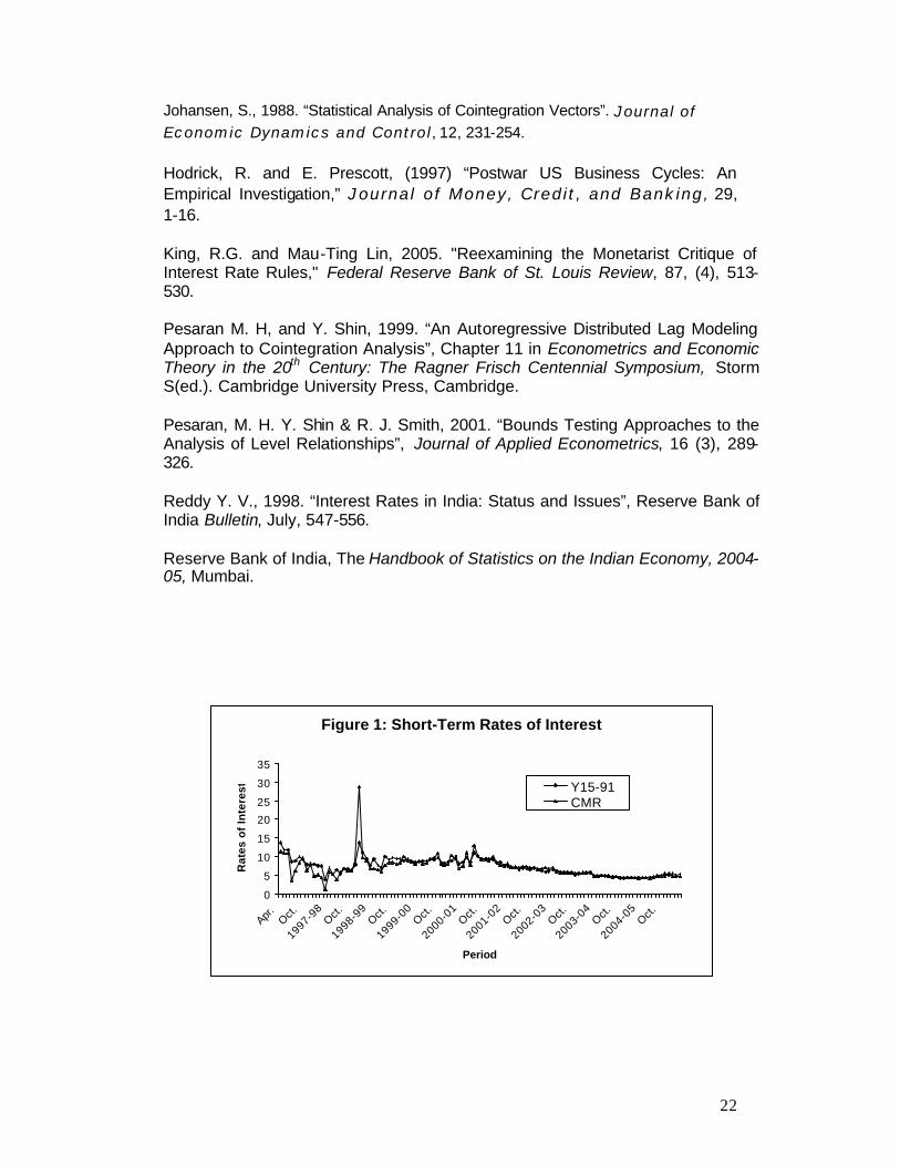
economy.1 The short-term interest rates plotted in Figure 1 show that there is a

downward trend of both call money rate and the 15 to 91 days Treasury bill rate.

It may be noted that in the initial years although there were some deviations

between the two rates, in the latter period both are moving closely. The medium

term and long-term rates on Government of India securities as shown in Figure 2

also show a declining trend. It may be noted that in the more recent period, all

the interest rates have started to show an upward trend. What then are the

factors that are leading to current rise in the yields. Is it due to domestic factors

or a response to the changes in the global financial market? This issue is

empirically explored while examining the determinants of interest rates in India.

In the subsequent section, we discuss the methodology for the analysis and

forecasting.

Methodology

For investigating the determinants of interest rates in India, this study follows the

cointegration approach. This is for the reason that the empirical research on

macroeconomic relationships, particularly when dealing with relatively higher

frequency data, would generally face the problem of non-stationarity. This

constrains the researchers in using traditional econometric tools like the OLS,

2SLS, etc. To solve the problem of non-stationarity, as a strategy the

cointegration approach has been developed (Engle and Granger 1987; Johansen

1988). The cointegration methods have been extensively used in the literature

over the last two decades in testing the long-run relationships. But these

methods suffer from some drawbacks. The basic condition for cointegration

analysis is that the variables in the system should be non-stationary at levels and

stationary of the same order. (The unit root tests that exist in the literature would

be used to determine the order of integration of the variables.) But quite often

1 For details regarding the policy changes with respect to interest rates in India, see Appendix-2

8

researchers face the problem that the results derived from the existing unit root

tests would differ depending on the power of the test. As a consequence, some

test statistics might be falling in the region of acceptance/rejection border. Given

this problem, in employing the cointegration technique, there exists scope for

bias in choosing the unit root tests that give the same order of stationarity for all

of the variables in the system. Further researchers also face the problem of

variables with a different order of integration. Therefore, it limits the use of

commonly used (traditional) cointegration analysis.

To overcome such a problem, Pesaran, Shin and Smith (2001) devised a bounds

testing autoregressive distributed lag (ARDL) approach to cointegration that

ignores the order of integration of variables. This ARDL-bounds testing method

can be applied for testing any long-run relationships irrespective of the variables

whether they are sta tionary at the same or different order. The technical details

regarding the ARDL model and its bounds test method are presented in

Appendix-1.

In the next stage, we discuss a framework for forecasting the interest rate cycle.

Most of the studies on interest rate forecasting either followed a macro-

econometric model or the pure time series model, depending upon the frequency

of the data. But as the short-term interest rates and their forecasting depend

more on short-term macroeconomic variables, it is not possible to construct a

macro-econometric (simultaneous equation) model. Further, as the variables

exhibit some sort of cyclical behaviour, it is not appropriate to apply time series

models without separating the cyclical and trend components from their observed

series. Hence, in this study, we decompose the series into trend and cyclical

components and then use appropriate forecasting techniques.

In any econometric exercise, first it is important to establish the time series

properties of the data. For this purpose, with the help of ADF and PP tests, we

examine whether the variables in question are stationary or non-stationary. In the

next stage, depending on the time series property, we decompose the series into

permanent (trend) and transitory (cyclical) components. If the series is stationary,

we follow the Hodrik-Prescot filter (1997). But if the series is non-stationary, we

9

follow the procedure developed by Beveridge and Nelson (1981), which is

discussed subsequently.

Beveridge-Nelson Procedure

Real macroeconomic time series variables are often decomposed into a

deterministic secular trend, a cyclical, and an irregular component. The deviation

around the trend forms a cyclical pattern and is ascribed as business cycle in the

literature. A typical economic cycle has a phase of upturn leading to the peak,

followed by a downturn ending up in a trough. To arrive at cycles, a real

macroeconomic time series is detrended by subtracting the trend value from

each actual observation and the irregular component in the detrended series is

smoothened by a 3-year or 5-year moving average. Even though it is a popular

method, it assumes that the variable is trend stationary. This is often not the

case, as a macroeconomic time series is often stochastic (random walk with a

drift). Further, incorporating a deterministic trend in a series with unit roots often

results in a misspecification error and the coefficients are statistical artifacts in

the presence of non-stationary error term (Enders 1995). Apart this, the forecast

function of a trend stationary model does not depend on current or past events.

Thus, when the trend part is stochastic (random walk with drift) then this

procedure is not appropriate. There are alternative methods of decomposition

when the series has a stochastic trend. One such method is the Beveridge and

Nelson (1981) decomposition method.

Beveridge and Nelson (1981) have developed a procedure to decompose a

series into permanent and transitory components. As the decomposition

procedure is useful only when the series is non-stationary at levels and stationary

at first differences, let yt be a non-stationary series. In the first stage, we estimate

the first differences of yt by using the Box-Jenkins method. Then the appropriate

ARMA model would be fitted and let that be a ARIMA(0,1,2). This can be

expressed as below.

∆yt = a0 + εt + β1εt-1 + β2εt-2 (1)

10

In the next stage, after estimating β, and a0 we obtain the in-sample forecasts of

each observation of yt and also the forecast errors, ε t. With the help of estimated

parameters and the forecast errors, one can estimate the irregular component of

the yt series as

C = -(β1+β2)εt - β2ε t-1 = yt - µ (2)

where, µ is a stochastic trend component in yt.

Hence, the non-stationary series yt is decomposed into the stochastic trend (or

permanent) component (µ) and the irregular (or transitory) component (C). Here

the irregular component is a stationary series and the permanent component

would be non-stationary series.

After decompos ing, we try to generate the out-of-sample forecast for the yt

series. For this purpose, we consider the trend/permanent component and the

irregular/transitory component separately. First, we examine the time series

properties of both the series and fit a suitable univariate model for both the series

separately for the best fit. In the next stage, we estimate the t+1 value of µ and

C. By adding these two values we get the necessary forecast value, i.e., 1ˆ +ty .

In this study, we use this decomposition method to forecast the various

secondary market interest rates in India. In the first stage, by using equations (1)

and (2), all the interest rate series are decomposed into permanent and transitory

components. After deriving the decomposed series, in the next stage, by looking

at the autocorrelation functions (ACFs) and partial autocorrelation functions

(PACFs), appropriate univariate models are used to forecast these series

separately.

But one of the limitations of the forecasts based on this univariate-decomposed

series could be that it does not take the exogenous variables into consideration

while forecasting. As the behaviour of macroeconomic variables might depend

on other variables in the system, the forecasts based on the univariate model

11

possibly might not be robust. Hence, to overcome this limitation, we forecast the

transitory component with the help of some macro variables. For this purpose,

we select the variables based on theory. We use the principle component

analysis to generate factors that explain the maximum variance of all the possible

variables. This also reduces the degrees of freedom problem in forecasting. With

the help of these generated factors we forecast the transitory components with

the help of the Vector Autoregression (VAR) model. The permanent component

would be forecasted by using the appropriate univariate model. The lag length for

the VAR model would be determined with the help of Schwartz Bayesian

Criterion (SBC). However, for an appropriate forecast, we have allowed flexibility

in using univariate and multivariate techniques. In the next section we discuss

the results.

Result Discussion

The correlation matrix presented in Table 1 shows that all the domestic interest

rates except the call money rate (which has a weak relationship), are significantly

correlated with the foreign interest rates and the exchange rate. While foreign

interest rate has a positive relationship, the exchange rate has a negative

relationship. However, it is surprising to observe that the inflation rate is not

correlated with any of the nominal yields. Besides inflation rate, the other

financial and real variables also do not exhibit a significant association with the

domestic interest rates. As the correlation coefficients do not capture the lead-

lag and cause-effect relationships between the variables, one needs to carry out

modelling exercise to examine the issues very clearly.

Table 1: Correlation Matrix of Domestic Interest Rates with Different Related Financial and Real Variables

ER FII FTBR3 FTBR6 LIBR3 GBC GIIP GWPILIBR3 -0.63 -0.36 1.00 1.00 1.00 0.03 -0.09 0.13

YIELD1 -0.63 -0.41 0.92 0.91 0.92 -0.07 -0.17 0.01

YIELD10 -0.72 -0.43 0.92 0.92 0.92 -0.17 -0.24 0.01

YIELD5 -0.77 -0.38 0.91 0.91 0.91 -0.16 -0.13 0.00

12

Y1591 -0.41 -0.37 0.78 0.77 0.77 0.10 -0.05 -0.01

CMR -0.12 -0.28 0.49 0.48 0.48 0.11 0.02 -0.05

While modelling through the time series analysis, for an appropriate time series

analysis, one requires to know the time series properties of all the variables

under consideration. Application of Augmented Dickey-Fuller test, for which the

results are presented in Table 2, shows that Y5, Y10, FII, GIIP and GWPI are

stationary in levels. The variables such as Y1591, Y1, ER, FPRM, FTB3, FTB6,

and LIBR3 although non-stationary in levels but are found to be stationary in their

first differences. Subsequently, the application of Phillips-Perron test confirms the

similar property of the variables. This shows that there is a presence of mixture of

both I(1) and I(0) variables.

After confirming the presence of I(0) and I(1) variables, we have applied the

ARDL approach to cointegration with different sets of variables along with the

presence of domestic interest rates as the dependent variable. Below we present

the results for the models, which have cointegration relationship. Table 3

presents the F-test for cointegration and the long run coefficients of the

corresponding cointegrating models. The F-statistics presented below show that

all the statistics cross the upper band of the critical values as tabulated by

Pesaran et al. (1999), rejecting the null of no cointegration in all the models. This

implies that there exists a long-run relationship among the variables in the

respective models. After ensuring the presence of cointegration, we have

estimated the long-run coefficients. The R-Bar square for the long-run estimates

shows that all the models are best fitting the data. They explain around 70 to 98

percentage of variation in the dependent variable.

Table 2: Unit Root Tests

ADF test Philips-Perron test Variables

In Levels In Difference In Levels In Difference Y1591 -3.09(2)

T -8.42(2)

N -4.38(2)

T -14.86(2)

N

Y1 -2.77(1)T -9.97(1)

N -3.08(1)

T -11.83(1)

C

Y5 -2.02 (1) N

-2.11(1) N

Y10 -2.13(1) N

-2.14(1) N

ERF -1.99(1) C

-4.55(3) N

-2.51(1) C

-7.56(3) N

CMR -5.09(1)

T -5.09(1)

T

13

FPRM -2.59(3) T

-7.02(2) N

-3.93(3) T -7.59(2)

N

FII -3.36(4)T -6.51(4)T

GIIP -3.80(1)T -4.50(1)

T

GWPIF -3.30(1)C -2.73(1)

C

FTBR3 -1.05(3)N -2.91(3)

C -1.10(3)

N -6.50(3)

N

FTBR6 -1.40(3)N -2.97(3)

C -1.07 (3)

N -6.30(3)

N

LIBR3 -1.02(3)C -2.77(3)

N -1.05(3)

N -5.50(3)

N

Note: The critical values at 1%, 5% and 10% are -3.494, -2.889 and -2.581 for with intercept but no trend and -4.049, -3.453 and -3.152 for with trend but no intercept and -2.587, -1.943 and -1.617 for no trend and intercept, respectively. The lag lengths for the tests are selected according to the minimum of AIC statistics. The trend and constant terms appear, when they are significant.

Where, T- refers to with trend and intercept, C - refers to no trend but with intercept

while N -refers to no trend and intercept. GIIP - Growth Rate of Index of Industrial Production FPRM - Forward Premium ERF - Expected Exchange Rate GWPIF- Expected Inflation Rate CMR - Call Money Rate GM3 - Growth Rate of Broad Money Supply FII - Foreign Institutional Investment FTBR3 - 3 monthly Federal Reserve Treasury Bill Rate FTBR6 - 6 Monthly Federal Reserve Treasury Bill Rate LIBR3 - 3 Monthly Libor Rate for US Currency Y1 - Yield on 1-Year Government of India Securities Y5 - Yield on 5-Year Government of India Securities Y10 - Yield on 10-Year Government of India Securities Y1591- Yield on 15 to 91 days Treasury Bill SP1591 - Yield Spread

The long-run estimates of the ARDL model shows that while the expected

exchange rate, expected inflation rate and foreign institutional investment exert a

negative influence the 6-monthly Federal Treasury Bill rate and the Spread rate

however, exert a positive influence on the call money rate. The real output, and

the money surprises do not have any significant impact. It is also noticed that by

replacing the money surprise with the growth of broad money supply and

considering either the Bank Rate or the Federal Funds Rate as exogenous policy

variable in the system, the estimation strategy does not improve on the

estimates. But when the 3-monthly Federal Treasury Bill rate is alternatively

replaced either with the 6-monthly Treasury Bill rate or 3-monthly LIBOR rate, the

sign of the estimates remain unchanged. They continue to exercise a positive

influence on the call money rate.

14

Considering the yields of 15 to 91 days Government of India's treasury bill as the

dependent variable in the system, it is seen that the real output has emerged to

have a negative influence along with the continuance of the negative influence of

the expected exchange rate and foreign institutional investment and the positive

influence of 3-monthly Libor rate and interest rate spread. Other variables, such

as expected inflation rate and replacement of forward premium with the expected

exchange rate variables do not produce any significant impact on the yields of

15-91 days Treasury bill. Similar to the above result, it is also seen that

incorporations of either Bank rate or Federal Fund’s rate, as an exogenous

variable do not improve the significance of the estimates. The result remains

invariant to the incorporation of alternative interest rate spread variables.

In contrast to the above results, which considered short-term interest rates; if one

considers the medium term rates, it is seen that yield on 1-year Government

Security is negatively influenced by the expected exchange rate, foreign

institutional investment and positively influenced by the 3-monthly LIBOR rate

and the interest rate spread. Other variables do not play any important role in

determining the annual yields on the Government of India security. In the case of

5-yearly Government of India Security, it is the only expected exchange rate that

has shown a significant and adverse impact on its yield (Y5).

Further, as regards the above results on short and medium term interest rates,

when one considers yield on 10-yearly Government of India's Security as a

dependent variable, it is found that while the expected exc hange rate, and

foreign institutional investment are consistent in exerting an adverse impact, the

3-monthly LIBOR rate is consistent in exerting a positive impact. The inclusion of

other variables except the alternative replacement of foreign interest rates does

not improve the results. All the foreign rates whether it is the 3-monthly or 6-

monthly Federal Treasury Bill rate or 3-monthly Libor rate, these continue to

exert a positive impact on the domestic interest rates in India. This corroborates

the findings of Dua and Pandit (2002). Looking at the error correction results, it

shows that while short-term rates in the subsequent period adjust at a faster rate

15

to any deviations from their equilibrium position in the previous period, the long

rates adjust to the disequilibrium very slowly to return to their equilibrium position.

Table 3: Estimated Long-Run Coefficients Using ARDL Approach to Cointegration

CMR Y1591 Y1 Y5 Y10 GIIP -1.48

[-1.27] -.33

[-6.73]*

ERF -.371 [-4.20]*

-.29 [-5.87]*

-.24 [-2.42]*

-.43 [-2.45]*

-.34 [-2.05]**

GWPIF -.323 [-2.81]*

-.098 [-.77]

LIBR3 .91 [16.27]*

1.02 [7.50]*

.92 [5.11]*

FTBR6 1.14 [8.12]*

0.97 [12.48]*

FII -.006 [-1.68]***

-.0009 -[4.14]*

-0.008 [-1.85]**

-.001 [-1.69]***

RESGM3 -.18 [-.97]

-0.019 [-.23]

GM3 -.12 [-.26]

.22 [1.48]

SP1591 1.76 [8.76]*

1.29 [10.69]*

.52 [3.02]*

.64 [1.46]

INPT 25.88 [5.42]*

21.34 [8.06]*

16.44 [3.34]*

28.26 [2.35]*

ECM -1 -.76 [-6.23]*

-.72 [-13.19]*

-.34 [-5.23]*

-0.54 [-2.14]*

-.14 [-2.90]*

R-Bar Square .70 .92 .95 .98 .98 Cointegration F- Statistic

4.23(2) 3.36(1) 3.59(1) 4.83(2) 3.65(2)

Note: * denotes significance at 1% level; ** denotes significant at 5% level, and *** denotes significant at 10% level. The parentheses relating to the F-statistics of cointegration test indicate the lag lengths considered in the above models.

From the above, the general conclusion that can be derived is that the expected

exchange rate and foreign interest rates do play a significant role in the

determination of interest rates in India. The magnitude of the foreign interest rate

is higher than the expected exchange rate. While the expected exchange rate

exercise an adverse impact, the foreign interest rates have a positive impact on

the domestic rates. The negative impact of the expected exchange rate on

domestic interest rates could be explained in that when we expect a depreciation

of the domestic currency, this leads to a greater demand for foreign currencies.

As a result, it gives rise to more inflows of foreign currency and a consequent

expansion of money supply in the domestic money market. This exerts a

downward pressure on the domestic rates of interest.

16

The above is also the reason why there is a negative impact of money surprises

on interest rates. But surprisingly, the growth rate of bank credit and broad

money supply do not play any role in influencing the interest rates in India. The

positive influence of the foreign interest rate on domestic interest rate may be

due to the competitive character of the financial environment and the central

bank's policy decision. It is also seen that while foreign institutional investment

has a negative impact on domestic interest rate; interest rate spreads have

positive impact on the domestic interest rates. Foreign institutional investment’s

negative influence on the domestic interest rate has the same reasoning as in the

case of the impact of depreciation of domestic currency on the domestic interest

rates. The more is the foreign institutional investment; the more is the expansion

in the level of money supply putting a downward pressure on the interest rate in

the economy. The interest rate spread has a direct relationship for the reason

that when interest rate on long-term maturity goes up, the short-term yields

follow. The output variable has an adverse impact only on the yields of 15 to 91

day treasury bills while the expected inflation rate has an adverse impact only on

the call money rate. Overall, it is found that the magnitude of impact of the

interest rate spread is higher than that of any other variable (surprisingly, except

the expected inflation rate in one case) irrespective of other domestic or foreign

variables. And among the foreign variables, it is the foreign interest rate, which

has a greater impact in terms of its magnitude.

Forecasting of Indian Interest Rate Cycle

As specified in the methodology section, this study tries to forecast the various

interest rates in a different way compared to Dua et al. (2003). In the first stage,

the actual observed series is decomposed into permanent and transitory

components by using B-N procedure or through the H-P filter, depending upon

the nature (stationary or non-stationary) of the series. As we found that Y1591

and Y1 are non-stationary and others are stationary variables (see Table 2),

therefore, Y1591 and Y1 are decomposed through the B-N procedure. The

permanent and transitory components are shown in Figure 3 and Figure 4. The

other variables are decomposed through the H-P filter and are presented in

Figure 5, Figure 6 and Figure 7. It may be visualized from the graphs that there is

17

no clear cyclical behaviour in the transitory components. The volatility has

declined since the beginning of 1999. In Figure 8 transitory components of both

Indian and foreign interest rates show that after 1999 the movements of these

interest rates are moving closer, if not at the same level. This supports our earlier

results that off late domestic interest rates are responding more to the

movements in foreign interest rates.

The permanent and transitory components are forecasted separately. The

forecasting models are presented in Tables 4 and 5. It may be noted that both

transitory and permanent components of the non-stationary series (Y1591 and

Y1) are predicted by using VAR models as the VAR model is found to give a

better fit. For the stationary series such as Y10 and Y5, VAR models are used to

predict the transitory components while univariate models are used to predict the

permanent components. This is because the transitory components showed high

volatility, which cannot be predicted using univariate models. In the case of CMR,

although both VAR and univariate models are not robust, the univariate models

are found to perform better as compared to the VAR models. Hence, both

transitory and permanent components of CMR are predicted using univariate

models. Here, for VAR models we are only presenting F-statistics, adj -R2 and

RMSE as the coefficients of individual variables are not important. Rather, a

collective significance (from F-statistic) of all the variables present in the model is

very important.

Table 4: Univariate Models Used for Interest Rate Forecasting

Dependent

Independent

CMRP CMRT Y10P Y5P

INPT 7.64 (13.93)*

3.79

(2.92)*

-0.06

(-2.83)* AR(1) 1.96

(163.43)*

0.64

(16.32)*

0.65

(4.78)*

1.91

(52.61)* AR(2) -0.97 -0.90 0.33 -0.95

18

(-81.38)* (-29.98)* (2.46)* (-25.73)* MA(1) 1.66

(30.62)*

-0.62

(-30.16)*

1.67

(28.05)*

1.17

(13.44)* MA(2) 0.84

(15.49)*

0.98

(1850.65)*

1.09

(24.54)*

0.53

(6.00)*

R-Bar Square .99 0.12 0.99 0.99 Note: The suffix P and T in each variable denotes permanent and transitory components. '*' Indicates significant at 1 % level.

Table 5: Multivariate (VAR) Models Used for Interest Rate Forecasting

Model (lag length) F-statistics Adj R2 RMSE

Y1T, FD1, FD2, FD3, FF1 (2) 3.6756* 0.27 0.19

Y1P, FD1, FD2, FD3, FF1 (2) 72.4855* 0.87 0.82

Y1591T, FFD1, FFD2, FFD3, FFD4 (2) 2.1473** 0.14 0.47

Y1591P, FD1, FD2, FD3, FF1 (2) 15.5075* 0.60 1.32

Y10T, FD1, FD2, FD3, FF1 (2) 10.6971* 0.47 0.29

Y5T, FD1, FD2, FD3, FF1 (2) 10.402* 0.46 0.32

Note: The suffix P and T in each variable denotes permanent and transitory components. '*' and '**' represents significant at 1 % and 5 % level respectively.

As explained in the earlier section, there are a number of possible factors that

explain the domestic interest rates. For any modeling purpose, it is not possible

to include all the variables at a time, although all are important. Hence, to

overcome such problem, the study reduces all the possible domestic variables

into three factors (FD1, FD2, FD3), which explains a 71.6 percent variation, by

using the principle component approach. In the case of three foreign variables,

we derived one factor (FF1) that explains 99.3 percent of variation in all the three

variables. We have derived the factors separately for the domestic and foreign

variables basically to examine the effects separately. Further, by mixing both

domestic and foreign variables, we derived four factors (FFD1, FFD2, FFD3,

FFD4) that explain a 76 percent variation. With the help of these factors and by

using the Vector autoregression model, we predicted the interest rates. The order

and structure of VAR models are chosen based on the predictive power in terms

of low root mean square error (RMSE). For all the yields, the model consisted

both domestic and foreign factors. In the case of CMR only, the model with

19

domestic factors showed low RMSE. The actuals and forecasts are provided in

Figures 9 to Figure 13.

It may be noted from Figure 9 to Figure 13 that the fitted models accurately

predict the in-sample behaviour (including the turning points) of all interest rates,

except in the case of CMR. The long cycles that we found in the yields are also

captured reasonably well. Given this performance of the models, it may be said

that the out-of-sample forecasts can be robust. From the out-of- sample

forecasts, it appears that the movement of interest rates would be upward from

now onwards. This is in consonance with our view that the domestic yield rates

respond majorily to the foreign rates, although with a significant lag. (From our

VAR results it was found that it takes 5 to 6 months for the domestic interest

rates to fully respond to movements in the foreign interest rates). Currently, as

the foreign interest rates are already moving up, our prediction of a rise in

domestic interest rates is highly feasible and also robust. Regarding the question

of the time and peaks in the level of future interest rate cycles, our results predict

that there will be peaks in each of the interest rates at different points of time.

Yield on the 15 to 91 day t-bills is expected to peak sometime in the first quarter

of 2006; one year yield is expected to peak in the second quarter of 2006; yields

on long term securities such as 5-year bond and 10-year bonds are expected to

peak in the fourth quarter of 2006. For the call money rate, as in the case of in-

sample, the out-of-sample forecasts are also very volatile. Also, as there is no

clear-cut cycle in the series, it is quite difficult to find out at what level it is going

to peak. Further, as the call money rate depends on various factors other than

the macroeconomic fundamentals, it may be difficult to predict its future

behaviour, particularly with a high frequency data.

Conclusion

The present study tries to examine the behaviour of various Indian interest rates

such as call money rate, and yields on secondary market securities with maturity

periods of 15 to 91 days, 1-year, 5-years and 10-years. In the first stage, the

study investigates the determinants of interest rates and finds that although the

20

interest rates depend on some domestic macroeconomic variables such as yield

spread and expected exchange rate, they are primarily affected by the movement

of international interest rates, although with a significant lag. The policy variables

such as Bank Rate and Federal Funds Rate did not show any significant impact

on any of the interest rates. The forecasts show that, except the call money rate,

all yields are expected to move upwards following the upward movement of the

international interest rate. Further, our results show peaks in each of the interest

rates at different time points. The yield on 15 to 91 day t-bills is expected to peak

sometime in the middle of 2006; the one year yield is expected to peak in the

third quarter of 2006; yields on long-term securities such as 5-year and 10-year

bonds are expected to peak in the fourth quarter of 2006.

The interest rate downturn, as witnessed since the year 2000, seems to have

ended in the middle of 2004. The upturn in the interest rates on Government

Securities started in the recent period is now likely to continue for at least about

two years. However, as reflected from its observed movement, it may taper off at

a peak much lower than the recorded during the high interest rate regime in mid-

1990s’. This may be because the government is adhering to its fiscal discipline

norms as set out in its Fiscal Responsibility and Budget Management Act (2003-

04) for achieving its targets in 2008-09. But three reasons can be cited which

might have contributed to the upward movement of domestic interest rates in the

recent years. First, the real interest rate seems to have reached the floor during

the industrial slow down of the early 21st century. There was only one possible

way to move from there on. Secondly, the industrial recovery from about 2003

onwards together with the rising international oil prices generated a rising

inflationary expectation which has also contributed to this upturn in the interest

rates. Finally, the persistence of a high fiscal deficit and the limit to the RBI

sterilization policy option has led to an increase in supply of government

securities corresponding to the demand. To some extent, the upturn is

restrained by easy liquidity created by the influx of foreign capital, especially in

the form of portfolio investments in government securities. The cyclical

movement in the interest rate during the market regime is not unexpected. It is

also to be noted that the floor of the interest rate in a developing country like

India is expected to be higher than that in rich countries with a surplus capital.

21

One obvious policy implication of this is that the soft interest rate regime

witnessed during the late 1990s and the early 21st century is now over. The

government would have to, therefore, borrow at a comparatively higher cost,

which means the government (both centre and state level) would have higher

interest costs on fiscal deficit. Second, the PLR on bank credit to the private

sector is now unlikely to go down because of the hardening of the interest rates

of Government Securities. The banks may have to, therefore, improve the

operational efficiency to restrict the rise in PLR. Finally, the integration of interest

rates in India, especially the yields on both short and lon-term Government

Securities, with the global interest rates imply that the Indian financial system will

now have a cyclical movement along with the global cycles. Hence, the Indian

financial markets cannot remain immune to global financial system. The policy

makers, therefore, have to take note of this in their monetary and fiscal policy

operations.

References

Beveridge, S. and C. R. Nelson, 1981. “A New Approach to Decomposition of Economic Time Series into Permanent and Transitory Components with Particular Attention to Measurement of the ‘Business Cycle,” Journal of Monetary Economics, 7, 151-74. Bhanumurthy, N. R. and S. Agarwal, 2003. “Interest Rate-Price Nexus in India”, Indian Economic Review, XXXVIII , (2), 189-203. Dua, P. and B. L. Pandit, 2002. “Interest Rate Determination in India: The Role of Domestic and External Factors”, Journal of Policy Modeling, (24), 853-875. Dua, P, Nishita Raje, & S. Sahoo, 2003. “Interest Rate Modeling and Forecasting in India”, DRG Study (24), DEAP, Reserve Bank of India. Edwards, S and M. S. Khan, 1985. “Interest Rate Determination in Developing Countries: A Conceptual Framework”, IMF Staff Papers, (32), 377-403. Enders, W., 1995. Applied Econometric Time Series Analysis. Engle, R. F. and C. W. J, Granger, 1987. “Co-integration and Error Correction Representation, Estimation and Testing”, Econometrica, 55, 251-276. Jha, R., 2002. “Downward Rigidity of Indian Interest Rates,” Economic and Political Weekly, 469-474.

22

Johansen, S., 1988. “Statistical Analysis of Cointegration Vectors”. Journal of Economic Dynamics and Control, 12, 231-254. Hodrick, R. and E. Prescott, (1997) “Postwar US Business Cycles: An Empirical Investigation,” Journal of Money, Credit, and Banking, 29, 1-16. King, R.G. and Mau-Ting Lin, 2005. "Reexamining the Monetarist Critique of Interest Rate Rules," Federal Reserve Bank of St. Louis Review, 87, (4), 513-530. Pesaran M. H, and Y. Shin, 1999. “An Autoregressive Distributed Lag Modeling Approach to Cointegration Analysis”, Chapter 11 in Econometrics and Economic Theory in the 20th Century: The Ragner Frisch Centennial Symposium, Storm S(ed.). Cambridge University Press, Cambridge. Pesaran, M. H. Y. Shin & R. J. Smith, 2001. “Bounds Testing Approaches to the Analysis of Level Relationships”, Journal of Applied Econometrics, 16 (3), 289-326. Reddy Y. V., 1998. “Interest Rates in India: Status and Issues”, Reserve Bank of India Bulletin, July, 547-556. Reserve Bank of India, The Handbook of Statistics on the Indian Economy, 2004-05, Mumbai.

Figure 1: Short-Term Rates of Interest

0

5

10

15

20

25

30

35

Apr.

Oct.

1997-98

Oct.

1998-99

Oct.

1999-00

Oct.

2000-01

Oct.

2001-02

Oct.

2002-03

Oct.

2003-04

Oct.

2004-05

Oct.

Period

Rat

es o

f In

tere

st Y15-91CMR

23

Figure 2: Long-Term Rates of Interest

0

2

4

6

8

10

12

14

16

Oct.

Mar

.Aug.

Jan.

Jun.

Nov.

1999-00

Sep.Feb.

Jul.

Dec.

May

Oct.

Mar

.Aug.

Jan.

Jun.

Nov.

2004-05

Sep.Feb.

Period

Rat

es o

f In

tere

st

Y1 Y5 Y10

Fig-3 Permanent and transitory components in Y15-91

-2

0

2

4

6

8

10

12

1997M

5

1997M

11

1998M

5

1998M

11

1999M

5

1999M

11

2000M

5

2000M

11

2001M

5

2001M

11

2002M

5

2002M

11

2003M

5

2003M

11

2004M

5

2004M

11

transitory permanent

Fig-4 Permanent and transitory components in Y1

-202468

101214

19

97

M5

19

97

M1

1

19

98

M5

19

98

M1

1

19

99

M5

19

99

M1

1

20

00

M5

20

00

M1

1

20

01

M5

20

01

M1

1

20

02

M5

20

02

M1

1

20

03

M5

20

03

M1

1

20

04

M5

20

04

M1

1

Transitory Permanent

Fig-5 Permanent and Transitory components in CMR

6

8

10

24

Fig-6 Permanent and Transitory components in Y5

-202468

101214

1997M

5

1997M

11

1998M

5

1998M

11

1999M

5

1999M

11

2000M

5

2000M

11

2001M

5

2001M

11

2002M

5

2002M

11

2003M

5

2003M

11

2004M

5

2004M

11

tranistory permanent

Fig-7 Permanent and Transitory components in Y10

-2

0

2

46

8

10

12

14

1997M

6

1997M

12

1998M

6

1998M

12

1999M

6

1999M

12

2000M

6

2000M

12

2001M

6

2001M

12

2002M

6

2002M

12

2003M

6

2003M

12

2004M

6

2004M

12

Transitory Permanent

25

Fig-8 Transitory components of Indian and foreign interest rates

-2.5

-2

-1.5

-1

-0.5

0

0.5

1

1.5

19

96

M1

1

19

97

M5

19

97

M1

1

19

98

M5

19

98

M1

1

19

99

M5

19

99

M1

1

20

00

M5

20

00

M1

1

20

01

M5

20

01

M1

1

20

02

M5

20

02

M1

1

20

03

M5

20

03

M1

1

20

04

M5

20

04

M1

1

Y15-91 FTBR3

fig-10 Actual and forecasts of Yield on 15-91 T-bills

Actual Forecasts

Fig-9 Actual and forecast of Call Money Rate

Actual Forecast

Fig-11 Actual and forecasts of Yield on 1 year G-sec

Actual Forecast

26

Appendix –1

Appendix-1

Appendix -1

Fig-12 Actual and forecast of Yield on 5 year G-sec

Actual Forecast

Fig-13 Actual and forecast of Yield on 10 year G-sec

Actual Forecast

27

ARDL Approach to Cointegration:

Let the unrestricted two variable VAR model in levels be;

t

p

jjtjt xx εµ +Φ+= ∑

=−

1

(1)

where xt is a (x1t,x2t), ì is vector of intercept and Öj is a matrix of unknown coefficients. And tε ~ IN(0,Ù) where ‘Ù’ is a positive definite matrix.

This procedure also assumes that both the series be purely I(1), or purely I(0) or cointegrated but excludes the possibility of seasonality roots and explosive roots.

Equation (1) can be expressed in the vector equilibrium correction model form in terms of long-run multiplier matrix and the short -run response matrix as below.

∑−

=−− +∆++=∆

1

11

p

jtjtjtt xxAx εγλ (2)

where Ä=1-L is the difference operator, and the short-run coefficient matrix is :

=

22

12

21

11

γ

γ

γ

γγ j ….. (3)

The long-run coefficient matrix would be

=

22

12

21

11

λ

λ

λ

λλ = ∑

=

Φ−−p

jjkI

1

)(

…………… (4)

Since the procedure focuses on conditional modeling of the scalar variable, x1t, we may express å 2t conditional in terms of å 1t as;

å 2t = tt u+Ω−2

12212 εω , (5)

where ut ~ IN(0, uuω ), uuω 211

221211 ωωω −Ω−≡ , and ut is independent of å 2t

Substituting equation (5) in (2), we get a conditional model for tx1∆ as,

∑−

=−− +∆′+∆′++=∆

1

12111211

p

jtttjtt uxxxAx ωϕλ (6)

To test for the presence of utmost one long-run relationship irrespective of the level of integration of x2, it is necessary to introduce a zero restriction on one of the off diagonals of the ë matrix. The procedure assumes that the k-vector ë21=0, which means that x1 has no long-run impact on x2. Under this restriction

∑−

=−− +∆++=∆

1

1221,22222

p

jtjtjtt xxAx εγλ (7)

In the same way, equation (6) would become

28

∑−

=−−− +∆′+∆′+++=∆

1

121,22,121,11111

p

jttjtjytt uxxxxAx ωϕλλ (8)

where 22122,12 λωλλ ′−≡

It may be noted from equation (7) -(8) that this restriction would not preclude the short-run causation between x1 and x2.

To test for the absence of the level relationship in the system, the procedure excludes the lagged level variables. Hence the null hypotheses would be

Ho : 02,1211 == λλ .

And the alternative hypotheses would be,

H1 : 02,1211 ≠≠ λλ . To test the hypothesis, we estimate equation (8) and calculate Wald or F-statistic. The asymptotic critical value bounds when the variables are I(0) and I(1) have been provided by Pesaran, Shin & Smith (2001). The decision rule for this procedure is if the estimated F-statistic falls below the lower critical value, we accept the null hypothesis that there is no long-run relationship. If the test statistic falls above the upper critical value, we reject the null hypothesis, i.e., there exists a long-run relationship between the variables. But if the test statistic falls within the critical value bounds, we cannot draw any conclusion at this juncture and we need further information about the order of integration of variables (Pesaran, Shin & Smith 2001). After ensuring that there is a presence of long-run relationship among the variables in the model, the second stage of the analysis is to estimate the coefficients of the long-run and short run relations and make inferences.

Appendix -2

Review of Policy changes in respect of Interest Rates in India: There are a number of reform measures undertaken in respect of interest rates for

imparting financial liberalization in the economy since the early 1990s. Along with a

phased reduction of the Statutory Liquidity Ratio (SLR), the deposit rates have been

simplified in 1991-92 by reducing the number of slabs. In 1994-95, the fixation of

minimum lending rates by banks for loans over Rs 2 lakh was no longer resorted to and

banks were allowed to fix their Prime Lending Rate (PLR) for advances over Rs 2 lakh.

The cooperative banks' lending and deposit rates were freed. The incremental SLR was

reduced to 25 percent along with reducing the base level SLR to 33.75 percent. The

CRR was reduced from 15 percent to 14 percent in 1995-96. In 1996-97, banks were

given the freedom to fix deposit rates for the term deposits above one year maturity.

CRR was reduced from 14 percent to 10 percent. Effective from April 1997, the Bank

Rate served as the signaling rate or reference rate linking it up with all other rates.

Banks were also conferred with the freedom to determine interest rates on term deposits

29

of 30 days and above. The entire structure of lending rates was deregulated along with

freedom given to the banks to offer fixed/floating PLR on loans of all maturities including

small loans upto Rs 2 lakh. The SLR was brought down to 25 per cent effective October

25, 1997. Interest rates on foreign currency deposits were to be determined by banks

subject to the ceiling rate prescribed by the RBI; these rates were subsequently linked to

LIBOR. With the supplemental agreement reached between the government and the

Reserve Bank of India (RBI), the issue of ad hoc Treasury bill was completely done

away with from April 1, 1997.

In 1998-99, banks were given the freedom to offer a differential rate of interest based on

size of deposits. Banks were advised to determine their own penal rates of interest on

premature withdrawal of domestic term deposits and NRE deposits. Banks were allowed

to charge an interest rate on loans against fixed deposits not exceeding its PLR. The

interim Liquidity Adjustment Facility (ILAF) was introduced in April 1999. This provided a

mechanism for liquidity management through a combination of repos, export credit

refinance and collateralized lending facilities (CLF) supported by open market operations

at set rates of interest. The savings deposit rates were reduced from 4.5 percent to 4.0

percent. The CRR was reduced from 10 percent to 9 percent. After the success of ILAF,

a full-fledged LAF was initiated on June, 2000. Interest rate in respect of repos and

reverse repos were decided through cut-off rates emerging from the auctions conducted

by the RBI on a uniform price basis. Banks were allowed to lend at sub-PLR rates. The

CRR was reduced to 8 per cent from 9 per cent along with a reduction of Bank rate from

8 percent to 7 percent.

In 2001, there was a further reduction of the CRR from 8 percent to 5.5 percent. The

Bank Rate was reduced from 7 percent to 6.5 percent. The Repo rate was reduced from

7 percent to 6 percent. The PLR of five major commercial banks declined from 11-12

percent to 10.75 to 11.50 percent in 2002-03. With effect from March 2003, the interest

rate on savings account offered by the banks was reduced to 3.5 percent per annum

from 4 percent annum. The CRR was reduced from 5.5 percent to 4.75 percent and

further to 4.50 percent in June 2003. The Bank rate was reduced from 6.5 percent to

6.25 percent. The Repo rate was reduced from 6 percent to 5 percent. The RBI had

reduced the interest rates on savings account, the only domestic deposit rate, which

continues to remain administered, reduced from 4.0 percent to 3.50 percent. In order to

provide consistency in interest rates offered to non-resident Indians, interest rates on

NRE deposits were linked to LIBOR/SWAP rates for US Dollar from July, 2003. Interest

rates on these deposits were reduced from 250 basis points above LIBOR/SWAP rates

30

to 100 basis points above LIBOR/SWAP rates effective from September 2003 and

further to 25 basis points above LIBOR/SWAP rates of corresponding maturity from

October 2003. From April, the above rates were further moderated to the LIBOR/SWAP

rate and it was stipulated that the interest rates on NRE savings deposits should not

exceed the LIBOR/SWAP rates for six-month maturity on the US Dollar deposits

The RBI has been following a policy stance of imparting flexibility to the interest rate

structure. Concerned over the downward rigidity of lending rates, even while deposit

rates were coming down, the RBI advised banks to announce their benchmark prime

lending rates (BPLRs) based on their actual cost of funds, operating expenses and a

minimum margin cover regulatory requirement. The BPLRs of five major banks are

lowered by 25 to 50 basis points in December 2004 compared to the rates prevailing

during 2004. In 2005, there is a marginal firming up of deposit rates by 25 basis points.

Call money rates firmed up from the 2nd half of the year, reflecting lower liquidity on

account of a large increase in bank credit. The bank rate remained unchanged at 6

percent. The repo rate (reverse repo rate) since October 2004, under LAF was raised by

25 basis points to 4.75 percent. The spread between reverse repo and repo was

narrowed by 25 basis points to 125 basis points. The CRR has moved from 4.50 percent

in January 2004 to 5 percent in January 2005.