Modeling interannual dense shelf water export in the ...klinck/Reprints/PDF/cougnonJGR2013.pdf · Modeling interannual dense shelf water export in the region of the Mertz Glacier

Modeling interannual dense shelf water export in the region of theMertz Glacier Tongue (1992–2007)

E. A. Cougnon,1,2,3 B. K. Galton-Fenzi,3,4 A. J. S. Meijers,5 and B. Legr�esy3,6

Received 28 January 2013; revised 23 August 2013; accepted 30 September 2013; published 28 October 2013.

[1] Ocean observations around the Australian-Antarctic basin show the importance ofcoastal latent heat polynyas near the Mertz Glacier Tongue (MGT) to the formation ofDense Shelf Water (DSW) and associated Antarctic Bottom Water (AABW). Here, we usea regional ocean/ice shelf model to investigate the interannual variability of the export ofDSW from the Ad�elie (west of the MGT) and the Mertz (east of the MGT) depressions from1992 to 2007. The variability in the model is driven by changes in observed surface heatand salt fluxes. The model simulates an annual mean export of DSW through the Ad�elie sillof about 0.07 6 0.06 Sv. From 1992 to 1998, the export of DSW through the Ad�elie (Mertz)sills peaked at 0.14 Sv (0.29 Sv) during July to November. During periods of mean to strongpolynya activity (defined by the surface ocean heat loss), DSW formed in the Ad�eliedepression can spread into the Mertz depression via the cavity under the MGT. Anadditional simulation, where ocean/ice shelf thermodynamics have been disabled, highlightsthe fact that models without ocean/ice shelf interaction processes will significantlyoverestimate rates of DSW export. The melt rates of the MGT are 1.2 6 0.4 m yr�1 duringperiods of average to strong polynya activity and can increase to 3.8 6 1.5 m/yr duringperiods of sustained weak polynya activity, due to the increased presence of relativelywarmer water interacting with the base of the ice shelf. The increased melting of the MGTduring a weak polynya state can cause further freshening of the DSW and ultimately limitsthe production of AABW.

Citation: Cougnon, E. A., B. K. Galton-Fenzi, A. J. S. Meijers, and B. Legr�esy (2013), Modeling interannual dense shelf water exportin the region of the Mertz Glacier Tongue (1992–2007), J. Geophys. Res. Oceans, 118, 5858–5872, doi:10.1002/2013JC008790.

1. Introduction

[2] Antarctic Bottom Water (AABW) is an important partof the global thermohaline circulation and is known to form inthe Weddell Sea, Ross Sea, and Ad�elie Land [Rintoul, 1998;Orsi et al., 1999; Jacobs, 2004]. More recently, AABW hasbeen observed to form in the vicinity of Cape Darnley, locatedimmediately west of the Amery Ice Shelf [Tamura et al.,2008; Kusahara et al., 2010; Fukamachi et al., 2010;Ohshima et al., 2013]. The Australian-Antarctic Basin (80�–

150�E) contains two types of AABW, defined by their sour-ces: Ross Sea Bottom Water enters the basin from the eastand mixes with Ad�elie Land Bottom Water that is formedlocally in geographically restricted latent heat polynyasaround the East Antarctic coastline [Rintoul, 1998]. AABW inthe Australian-Antarctic Basin has been observed to be fresh-ening, possibly due to an increased supply of glacial melt-water from Antarctica [Aoki et al., 2005; Rintoul, 2007].

[3] The high rate of sea ice formation in latent heat poly-nyas and the associated brine rejection drive convectiondue to the formation of relatively dense water (e.g., HighSalinity Shelf Water—HSSW). HSSW can sink below ad-jacent ice-shelves and drive basal melting of these ice-shelves leading to the creation of fresher Ice Shelf Water(ISW), which is defined as having a temperature below thesurface freezing temperature [Lewis and Perkin, 1986]. Themixture of HSSW, ISW, and to some degree the overlyingCircumpolar Deep Water (CDW) and Modified Circumpo-lar Deep Water (MCDW) can form Dense Shelf Water(DSW). DSW may be exported from the continental shelf,sinking into the deep ocean and mixing further with theMCDW, forming AABW. Changes in the volume of ISWand HSSW formed on the shelf can significantly alter sub-sequent formation rates of AABW at the continental shelfbreak [Hellmer, 2004; Kusahara and Hasumi, 2013].

[4] During the period of this study (1992–2007), theMertz Glacier Polynya (MGP), centered at about 67�S and

1CSIRO-UTAS Quantitative Marine Sciences PhD Program, Institutefor Marine and Antarctic Studies, University of Tasmania, Hobart, Tasma-nia, Australia.

2Commonwealth Scientific and Industrial Research Organisation, Ma-rine and Atmospheric Research, Hobart, Australia.

3Antarctic Climate & Ecosystems Cooperative Research Centre, Uni-versity of Tasmania, Hobart, Tasmania, Australia.

4Australian Antarctic Division, Kingston, Tasmania, Australia.5British Antarctic Survey, Cambridge, UK.6Laboratoire d’Etudes en G�eophysique et Oc�eanographie Spatiales

(CNES-CNRS-UPS-IRD), UMR5566, Toulouse, France.

Corresponding author: E. A. Cougnon, CSIRO-UTAS Quantitative Ma-rine Sciences PhD Program, Institute for Marine and Antarctic Studies,University of Tasmania, Private Bag 129, Hobart, Tas 7001, Australia.([email protected])

©2013. American Geophysical Union. All Rights Reserved.2169-9275/13/10.1002/2013JC008790

5858

JOURNAL OF GEOPHYSICAL RESEARCH: OCEANS, VOL. 118, 5858–5872, doi:10.1002/2013JC008790, 2013

145�E, was the second largest polynya in area (23,300km2) along the East Antarctic coastline [Massom et al.,2001] and was a key source of DSW that ultimatelybecomes AABW [Rintoul, 1998; Williams and Bindoff,2003; Williams et al., 2008]. From satellite remote sensingobservations, the MGP is estimated to produce an annualcumulative volume of sea ice of about 120 6 11 km3 yr�1

[Tamura et al., 2008]. The factors that influence the iceproduction of the MGP are the steep ice-sheet topographyinland from Commonwealth Bay and Buchanan Bay(Figure 1) that funnel strong and persistent katabatic windsinto the area, the distribution of grounded icebergs and sur-rounding fast ice, and the position of the Mertz Glacierfloating ice Tongue (MGT) and other icebergs (like thelarge grounded iceberg B9b) which form a barrier againstwestward moving sea ice [Massom et al., 2001]. The MGTwas 20–40 km wide and extended 150 km northward fromthe grounded ice-sheet, prior to its calving in 2010, whichcut its length in half.

[5] Direct observations of the ocean in the vicinity of theMGT during winter are rare, due to the extreme conditionsmaking access difficult. The first and the only wintertimeexperiment in the Ad�elie region occurred in July to August1999 [Bindoff et al., 2001; Williams and Bindoff, 2003;Williams et al., 2008]. This wintertime experiment andassociated summer observations have shown that DSWaccumulates in the Ad�elie depression, and the Ad�elie sill isone of the primary outflow regions for dense water toescape from the depression to the abyssal ocean [Bindoff et

al., 2000; Williams et al., 2008]. The annual mean exportof DSW through the Ad�elie sill was estimated to be 0.1–0.5Sv [Williams et al., 2008], subsequently revised down to0.073 6 0.083 Sv using improved analysis methods(Meijers et al., manuscripts in preparation). DSW exportedat the sill depth (425 m) is dense enough relative to the off-shore water masses to mix down the continental slope andslope canyons to form AABW [Williams et al., 2008].More recent observations taken along the slope and overthe deep ocean suggest that the Mertz sill, to the east of theMGT, may also be a region of DSW export [Williams etal., 2010]. The region to the east of the MGT also has adeep depression, called the Mertz depression or Trough, asill (600 m) and an active local polynya in the lee of B9b.Modeling results also support the hypothesis that the Mertzsill is a key region of DSW export from the Mertz depres-sion to the continental slope [Kusahara et al., 2011].

[6] Earlier model studies such as Marsland et al. [2004]using the Mertz-HOPE (Hamburg Ocean Primitive Equa-tion) model (as described by Marsland et al. [2007]) andKusahara et al. [2011] using the Center for Climate SystemResearch Ocean Component (COCO) model [Hasumi,2006], have studied the Ad�elie/Mertz depressions area.Both are coupled sea-ice/ocean models and have a globaldomain with high horizontal resolution over the study area.Neither of these studies include ice shelf/ocean interactionprocesses the circulation underneath ice-shelves or the for-mation of ISW. Our study uses a high resolution (�2.16–2.88 km) regional ocean model, based on the Regional

AB MB

ADMD

MSAS

DDU CB WB

MGT

Fast ice

Fast ice

Cook ice shelfNinnis

ice shelf

Ninnis icebergs

B9b

Figure 1. Bathymetry of the model and features of note around the Ad�elie and Mertz depressions. Inthe ocean: (AB: Ad�elie Bank; AD: Ad�elie Depression; AS: Ad�elie Sill ; MB: Mertz Bank; MD: MertzDepression; and MS: Mertz Sill), with the ice draft (dark line) of the Mertz Glacier Tongue (MGT; 140km long, 25 km width), the B9b (with a draft of �300 m) and of the fast ice (� 30 m thick for the fastice south east of the MGT and � 10 m for the fast ice south east of B9b). Along the continent : WattsBay (WB), Commonwealth Bay (CB), and Dumont D’Urville base (DDU). Cyan, green, and blue dashedlines indicate the boxes (Ad�elie, Mertz, and MGT boxes), used for averaging model results. The easternedge of the cyan box is partially obscured by the green box and the yellow line. Cyan and green boldlines show the Ad�elie and Mertz sill section, respectively, and the yellow bold line along the MGT showsthe cavity section.

COUGNON ET AL.: MODELING INTERANNUAL DENSE SHELF WATER

5859

Ocean Modeling System (ROMS) [Shchepetkin andMcWilliams, 2005] to study the interannual variability ofDSW export from the Ad�elie and Mertz depressions regionfrom 1992 to 2007. The model is unique in that it has beenmodified to include ice shelf/ocean interactions and frazildynamics and thermodynamics, and includes the oceancavity beneath the MGT and other ice-shelves, icebergs,and fast ice in the region [following Galton-Fenzi, 2009,2010; Galton-Fenzi et al., 2012]. Marsland et al. [2004]have shown a strong interannual variability of DSW out-flow from the Ad�elie depression linked to variability inatmospheric forcing. In this study, we investigate the linkbetween the variability of the surface polynya forcing andthe shelf water, and how it impacts the density and volumeof exported DSW.

[7] Section 2 describes the model setup and forcing, anddetails the analysis procedure. A similar approach to Mars-land et al. [2004], using heat flux variability, is used in sec-tion 3 to define different polynya states. Using thesepolynya states, we examine relationships between the in-tensity of polynyas and dense water export, and the interac-tions with the ice shelf. In sections 4 and 5, we discuss keyfindings relating to dense water export. These include thedifferent pathways for DSW export and the importance ofincluding the cavity under the MGT, as well as the linkbetween polynya activity and DSW export in comparisonwith previous model studies.

2. Methods

2.1. Model and Forcing

[8] The three-dimensional ice shelf/ocean cavity modelused here is based on the Rutgers version of the RegionalOcean Modeling System (ROMS) [Shchepetkin andMcWilliams, 2005]. ROMS has a free surface and uses aterrain-following vertical s-coordinate system controlled bythe applied surface pressure, which has been adapted toallow the coordinates to follow the ice-shelf draft [Dinni-man et al., 2003] and has been applied to other area of Ant-arctica [Dinniman et al., 2007; Mueller et al., 2012]. Theversion of the model we use here was initially developedfor studies of the Amery Ice Shelf/Ocean system [Galton-Fenzi, 2009; Galton-Fenzi et al., 2012] and used incircum-Antarctic modeling studies [Galton-Fenzi, 2010].In the region of our study, a version of this model has beenused to simulate the circulation patterns and water massproperties in the vicinity of the Ad�elie and Mertz depres-sions [Hemery et al., 2011; Cottin et al., 2012]. It has alsobeen compared directly with summertime ship observationsand year long current meter moorings at the Ad�elie sill andfound to accurately reproduce the seasonality and circula-tion within the depression (Meijers et al., manuscripts inpreparation).

[9] The model setup used here is similar to the onedescribed by Galton-Fenzi et al. [2012] and only the majorfeatures and differences from the previous model aredescribed below. The model includes realistic tides andthermodynamic interactions with the ice shelf, includingthe addition of a frazil subroutine. The ice shelf/oceaninteraction is described by three equations representing theconservation of heat, salt, and a linearized version of thefreezing point of seawater (as a function of salinity and

pressure) [e.g., Holland and Jenkins, 1999], which aresolved to simultaneously find the temperature and salinityin the boundary layer beneath the ice shelf and the meltrate at the ice shelf base. The model grid extends from135.77�E (west of the French base Dumont D’Urville) toeast of George V land at 158.08�E and covers the Ad�elieand Mertz depressions from the coast line up to the deepocean at 62.72�S (Figure 1). The horizontal grid has a reso-lution of about 2.16 km near the southern boundary and2.88 km near the northern boundary. The vertical grid uses31 contour following � levels, arranged to give higher reso-lution near the top and the bottom of the water column.

[10] The bathymetry and ice-shelf draft is based onRTopo-1 [Timmermann et al., 2010] and was modified toinclude local high-resolution bathymetry data from Bea-man et al. [2011], which is based on multibeam swath so-nar and singlebeam bathymetry data with about 250 mresolution. The iceberg positions present in the region,and the MGT ice draft were created using high-resolutionSPOT5 imagery, radar profiles from Legr�esy et al. [2004],and a more recent airborne radio echo sounding (ICECAPproject from International Polar Year and Greenbaum etal. [2010]). The bathymetry beneath the MGT has beencreated to accommodate the grounding line position andits thickness [Legr�esy et al., 2004; Mayet et al., 2013].The ice draft of the MGT is shown in Figure 5, while theB9b icebergs have a draft of 300 m and Ninnis icebergshave a comparable thickness. Fast ice is an important fac-tor to consider in the region because of its thickness andits multiannual presence in some areas [Massom et al.,2009]. We include a climatology from Fraser et al.[2012], which produces two main areas of permanent fastice near the MGT. These regions are southeast of the icetongue and southeast of the B9b iceberg, where fast ice iscontinuously present with a relatively constant area (seeFigure 1). Southeast of the MGT fast ice attached to theglacier tongue is relatively old (at least 25 years) and thick(from 10 to 55 m). This is about 10 times thicker than themean thickness of pack ice in the region [Massom et al.,2010].

[11] Following Galton-Fenzi et al. [2012], the model isforced with monthly data over the period from January1992 to December 2007. Previous studies highlighted theimportance of small-scale features, such as grounded ice-bergs, many of which are only a few hundred meters inscale. These features are important for the formation ofpolynyas and lead to localized enhanced DSW production[Kusahara et al., 2010]. However, coastal polynya andicebergs are often poorly resolved or are not parameter-ized in models, and so no sea ice model is coupled to theocean in the present study. Instead, heat and salt fluxes,based on ice concentration from a climatology derivedmodel using Special Sensor Microwave Imager (SSM/I)observations from 1992 to 2007 [Tamura et al., 2008,2011], are used to adequately resolve the fine-scale poly-nya in the region, as has been done for other similar stud-ies as Dinniman et al. [2003, 2007]. During summer, theTamura et al. [2008] data are supplemented with open-water heat and salt fluxes using monthly climatologiesfrom NCEP-2 [Kanamitsu et al., 2002]. Surface winds arederived from the second version of CORE data developedby Large and Yeager [2009] for global ocean-ice


5860

modeling [Griffies et al., 2009]. The surface kinematicwind stress, � , is calculated in the i direction and j direc-tion from the wind velocity field, u as:

� i;j ¼ �acaui;jjui;jj

where �a is the air density (1.3 kg m�3) and ca is the dimen-sionless air-sea friction coefficient (1.4 � 10�3). Lateralboundary fields, including potential temperature, salinity,and horizontal velocities are relaxed to monthly fields fromECCO2 over the period [Menemenlis et al., 2008; Wunschet al., 2009]. The model was run for 48 years, including aspinup phase of 32 years to reach equilibrium using arepeating loop of synoptic forcing from 1992 to 2007. Thefinal 16 years are used in the analysis.

2.2. Analysis Regions and Experiments

[12] To investigate the exchange between both shelfdepressions and the export of DSW over the shelf break,our analysis is focused on three boxes around the Ad�elieand Mertz depressions and the MGT (Figure 1), and onthree sections at the Mertz and Ad�elie sills and at the MGTcavity. These regions are chosen so as to facilitate compari-sons with other studies [Marsland et al., 2004; Kusahara etal., 2011; Meijers et al., manuscripts in preparation]. Thevariables that are examined are potential temperature, sa-linity, horizontal velocities, and the volume transport of themain water mass classes (defined below). The boxes chosencompletely surround the MGT in order to investigate thecirculation through the cavity and ISW formation. Theyalso include both the Ad�elie and Mertz depressions andtheir corresponding polynya areas, where the formation ofshelf water occurs, and finally include both sills, where theexport of DSW from the depressions is thought to occur[Williams et al., 2010; Kusahara et al., 2011].

[13] Different types of water interact within our studyarea, coming from offshore or forming over the shelf(Table 1). Antarctic Surface Water (AASW) is relativelywarm and is the least dense water mass in the region,appearing at the surface. Below the surface offshore thereis warm and saline CDW, and the deepest water mass offthe shelf break is AABW. CDW moves southward andbecomes Modified CDW (MCDW) through mixing withAASW and water over the shelf, before crossing the shelfbreak and entering the shelf region in the mid-water col-umn where it can interact with HSSW and ISW createdduring sea ice formation and ice tongue melting, respec-tively. Low Salinity Shelf Water (LSSW) corresponds to awater mass similar to the HSSW in potential temperaturebut with a salinity less than 34.5 psu. We define DSW hereas any water having a potential density greater than1027.88 kg m�3. This potential density has been used inprevious studies as being the minimum potential densitycapable of sinking off the shelf and reaching abyssaldepths, eventually contributing to the formation of AABW[Bindoff et al., 2001; Williams et al., 2008; Kusaharaet al., 2010].

[14] To highlight the importance of considering ocean/ice shelf thermodynamics in modeling studies of shelfprocessed and dense water export, two experiments are per-formed for this paper: (1) ‘‘Reference simulation’’: the ref-erence simulation uses the best version of the model

described above, including ice shelf/ocean thermodynam-ics. (2) ‘‘Without ice shelf thermodynamics’’: referencesimulation, but without ice shelf basal melting/freezing, sono ISW will be generated.

3. Results

3.1. Polynya Activity

[15] The 16 year time series of heat fluxes from Tamuraet al. [2008, 2011] shows an interannual variability in poly-nya activity (intensity) in the region (Figure 2). This figureshows the cumulative heat flux anomalies and the averagewintertime heat flux anomalies for a fixed size area includ-ing both the Ad�elie and Mertz depressions (black line). Italso shows those anomalies for smaller areas, one centeredon the Mertz Glacier Polynya (MGP) over the Ad�eliedepression (dashed line) and the other on the polynya in thelee of B9b iceberg over the Mertz depression (dotted line).The polynya activity is slightly different between the MGPand the region over the B9b polynya, but not dramaticallyso. For simplicity, we define the state of polynya activity aschanges over the combined area of the depressions. The cu-mulative heat flux anomalies from monthly means over theAd�elie and Mertz depressions (Figure 2a), shows a suddenchange in polynya activity occurring in 2002. A positivecumulative flux trend indicates that the flux of heat fromthe ocean to the atmosphere is less than the normal trendover the whole period, and therefore indicates a decrease inpolynya activity. A negative trend in polynya activity indi-cates intensified heat loss and increased polynya strength.In Figure 2a, interannual variability is observed with a netincreased cumulative flux from 1999 to 2001 inclusive(about þ550 MJ m�2) with a sudden change in 2002 and astrong decrease of the cumulative flux until 2004 (about�600 MJ m�2). From 1992 to 1996, the cumulative heatflux anomalies are relatively constant before increasingfrom 1997 to 1999 (þ300 MJ m�2), although at a weakerrate than from 1999 to 2001.

[16] The average heat flux anomalies (Figure 2b) for thewintertime average (from May to September inclusive)show the same pattern in terms of interannual variability,with the same two key periods of polynya activity. The pe-riod from 1999 to 2001 inclusive has a wintertime positiveheat flux anomaly of approximately 8 6 4 W m�2, corre-sponding to a ‘‘weak polynya state.’’ The period from 2002to 2004 inclusive has a wintertime negative heat flux anom-aly of approximately �11 6 3 W m�2, corresponding to a‘‘strong polynya state.’’ It is more difficult to define persis-tent strong or weak states for the other years because

Table 1. Water Masses Defined by Potential Temperature (�), Sa-linity (S), and Potential Density (�)

Water Type � (oC) S (psu) � (kg m�3 �1000)

AASW �1.75� �� 2 �� 27.75MCDW �1.75� �< 1 27.75<�< 27.88HSSW fpa<�<�1.75 S> 34.5LSSW fpa<�<�1.75 S� 34.5ISW �� fpa

DSW �� 27.88

afp is the in situ freezing temperature of sea water at 50 dbar.


5861

negative heat flux anomalies alternate with positive anoma-lies each year, corresponding to a constant cumulative heatflux. We therefore call the period from 1992 to 1998 the‘‘mean polynya state.’’ Marsland et al. [2004] defined simi-lar periods in polynya activity for the years in which thestudies overlap (1992–2001). They defined a strong poly-nya state from 1993 to 1999, corresponding to the ‘‘mean’’polynya state in our study, and weak polynya years (1999and 2000) corresponding with our weak polynya state. Asour study is longer, we define another period of ‘‘strong’’polynya activity from 2002 to 2005.

3.2. Transport From the Ad�elie and MertzDepressions

[17] The export by time for each density class between1027.65 kg m�3 and 1028.00 kg m�3 is shown in the col-ored plots of Figure 3. The export is binned in densityincrements of 0.01 kg m�3 for the Ad�elie and Mertz boxesand both sills. This export is calculated as monthly aver-ages over the entire period (from 1992 to 2007). The criti-cal DSW density limit (1027.88 kg m�3) is represented bythe horizontal dashed line. Figure 3 clearly shows interan-nual variability in the export of DSW for both depressionsand sills, but also seasonal variability. The minimum den-sity for exported water is denser at the end of each winterand slightly lighter during summer, and does not always

exceed the critical value. Over the 16 study years, three dis-tinct periods of DSW export can be defined, as indicated bythe vertical dashed lines. The first period is from 1992 to1998, where the DSW export is strong for the Ad�elie box,and the two sills, associated with an import of the densestDSW into the Mertz box. 1999 is a transition year withlighter water exported, too light to be considered DSW butdense enough to be still exported from the Ad�elie box. Thistransition period is followed by a second period from 2000to 2002, where there is almost no export of DSW from anyof the boxes and sections. The last period is from 2003 to2005 where there is an increase of DSW export mainlyseen to flow out of the Ad�elie box and circulate through thecavity to the Mertz box. These periods lag the previouslydefined periods of polynya activity (shown by the arrows inthe figure) by about a year.

[18] Different water masses can share the same densitycharacteristics, so it is therefore useful to consider thetransport results presented in Figure 3 together with poten-tial temperature and salinity characteristics to determinethe transport pathways of each of the main water masses.Figure 4 shows the net transport across both boxes and sillsbinned by potential temperature and salinity, averaged overthe periods 1992–1998, 2000–2002, and 2003–2005. Thisprojection allows us to see the different water masses thatenter and exit each depression. The different water masses

Figure 2. (a) Cumulative heat flux anomalies for the shelf fixed size area including both the Ad�elie andMertz depressions (black line), for a small fixed size area over the Ad�elie depression (Mertz Glacier Poly-nya, dashed line), and a small fixed size area over the Mertz depression (B9b polynya, dotted line). Verti-cal dashed lines show the different states in polynya activity described in the text. (b) Heat flux anomaliesfor monthly means from Tamura et al. [2011] (fine gray line) and wintertime averages from May to Sep-tember inclusive over the shelf area including both Ad�elie and Mertz depressions (black line with dots),the Ad�elie depression (Mertz Glacier Polynya, dashed line), and the Mertz depression (B9b polynya, dot-ted line). Negative anomalies indicate increased polynya strength and Dense Shelf Water formation.


5862

defined in Table 1 are labeled in Figure 4a, and we focuson the variability of the four main water masses: MCDW,HSSW, ISW, and DSW. ISW is defined here to be colderthan the freezing temperature of sea water at 50 dbar. Usinga depth below the surface is a necessary condition so thatvery shallow ISW produced by melting of thick fast iceeast of the MGT (at about 35 m) is excluded. The averagedtransport for each water mass (in 103 m3 s�1 or milli-Sverdrups) and period for the Ad�elie and Mertz boxes andsills, and also for the cavity are summarized in Tables 2a–2c. Averages are also calculated for each case during theannual ‘‘peak export’’ period, which is defined as July toNovember, following Marsland et al. [2004] and whichalso corresponds to the peak dense water formation fromobservations [Williams et al., 2008].

[19] The density transport for both the Ad�elie and Mertzdepressions differs between each period. However, in allthree periods there is an import of relatively warm MCDW(between 0�C and 0.5�C, see Figures 4a–4c and 4g–4i)with a density between1027.80 kg m�3 and 1027.85 kgm�3. For the Ad�elie box, an export of water denser than1027.85 kg m�3 (dense enough to exist below the importedMCDW) is seen for both the first period (1992–1998) andthe last period (2003–2005). This contributes to an exportof DSW of 378 mSv for the first period and of 273 mSv forthe last (Table 2a). During the first period, 29% of theDSW exported from the Ad�elie depression flows outthrough the Ad�elie sill (110 mSv), while only 19% goesthrough the sill during the last period (51 mSv). During thesecond period, the export is less dense, more spread in

terms of density and salinity, and is only marginally denserthan the imported water, so there is very little net DSWexported through the sill (<30 mSv).

[20] An export of very salty and dense HSSW isobserved from the Ad�elie box with a transport of 212 mSvand 159 mSv for each period, respectively. This export hasthe same characteristics as the very dense water importedinto the Mertz box (Figures 4g–4i). The circulation throughthe cavity section makes up a large proportion of the totalDSW transport: 43% of the exported DSW formed in theAd�elie depression is going through the cavity (165 mSv)during the first period and 46% (127 mSv) during the lastperiod. This implies that 28% of DSW formed in the Ad�eliedepression during the first period and 35% during the lastperiod exits the box through pathways other than beneaththe cavity or through the sill. These other pathways are dis-cussed further in section 4.2.

[21] DSW that circulates beneath the MGT from theAd�elie depression appears as an import into the Mertz boxand is the sole pathway of DSW into the Mertz box throughlateral boundaries. The 120 mSv exported out of the Mertzbox are formed in the Mertz depression, primarily from thepolynya in the lee of B9b, which is two third less than theDSW produced in the Ad�elie depression. The distribution ofthe water exported through the Mertz sill, in terms of density,shows a small import of MCDW (Figures 4j–4l), coupledwith an export of cooler MCDW. Also, 207 mSv of DSW isexported through the sill during the first period significantlymore than the net depression export. During the last period69 mSv of DSW goes out through the Mertz sill, while the

lliS eilédA )bxoB eilédA )a

c) Mertz Box d) Mertz Sill

Figure 3. Transport (in Sv) by potential density class (in kg m�3 �1000) for each box and sill. Posi-tives values (red) correspond to an export ; negative values (blue) correspond to an import. Horizontaldashed line is the critical density 1027.88 kg m�3. Vertical dashed lines show the limits of differentstates of DSW export, as discussed in the text. The arrows at the top of each plot show the transitionbetween polynya activity states.


5863

global DSW transport over the entire Mertz box shows animport of 35 mSv. This highlights the importance of theAd�elie depression as the primary source of DSW and of the

circulation beneath the MGT. During the second period,associated with weak polynya forcing, there is only a weakexport of DSW (<50 mSv) from the whole Mertz box.

AASW

LSSW

MCDW

HSSW

ISW

1992 - 1998 2000 - 2002 2003 - 2005

a) )c)b

)f)e)d

g) h) i)

j) )l)k

(mSv)

Figure 4. Potential temperature-salinity transport diagrams for the (a, b, c) Ad�elie box and (d, e,f) sill, and (g, h, i) Mertz box and (j, k, l) sill, split by period. Positive values (red) correspondto an export, and negative values (blue) correspond to an import (in milli Sv). Water masses areshown on the top left plot. Some potential density contours are shown on each diagram, with adashed line corresponding to the freezing temperature of sea water at 50 dbar, used to defineISW in this study.


5864

3.3. Transport and Melting in the Mertz GlacierTongue Cavity

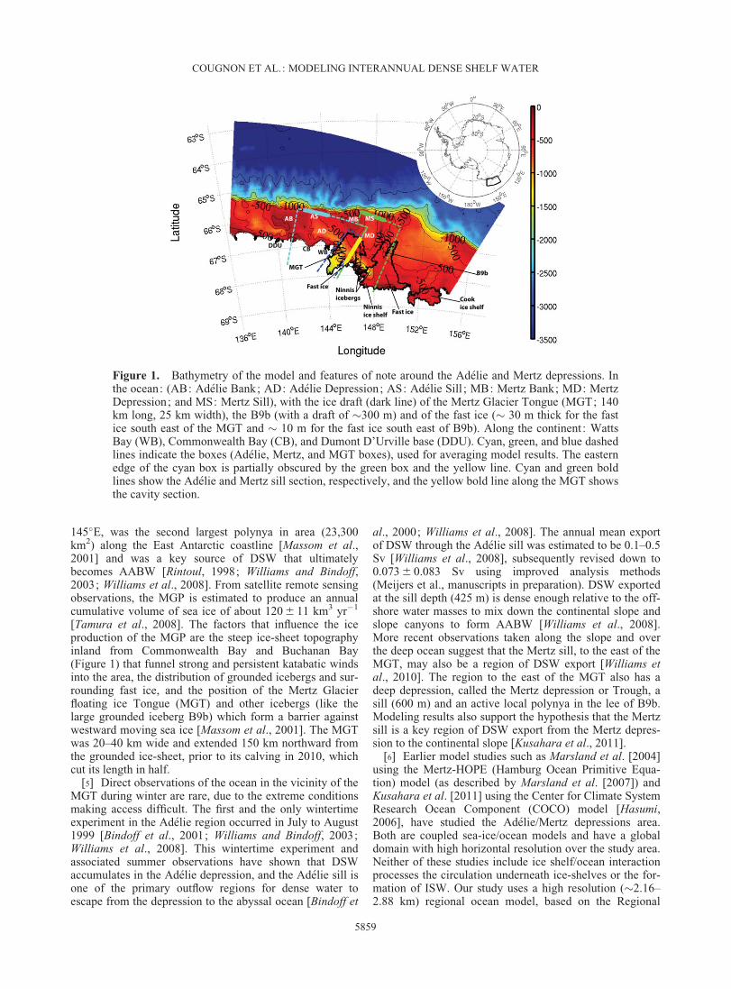
[22] In this section, we examine the transport through thecavity. DSW formed in the Ad�elie depression flows intothe MGT cavity on its western side, interacting with the iceshelf and mixing with ISW, leading to an export of slightlyfresher and lighter water into the Mertz depression from theeastern side of the MGT. The difference between the sec-ond (weak) and the first (mean) periods in � and S along thesection defined by the MGT box are shown in Figures 5aand 5b. The third period (strong) is similar to the first, soanomalies from this period are not shown. The second pe-riod is mostly fresher and warmer everywhere along thesection, except at about 400 m along the northern part ofthe MGT where a warm and salty anomaly occurs (of aboutþ1�C and þ0.04 psu). The perpendicular velocity acrossthe MGT transects over both periods (Figures 5c and 5d)shows a corresponding change in the circulation and mag-nitude along the northern part of the MGT at about 400 m.Import into the cavity at depth increases on the westernboundary of the MGT, and a current can also be seen cross-

ing the northeasterly tip of the MGT, heading in a southeas-terly direction between 400 and 600 m. This is indicativeof an import of MCDW under the northern part of theMGT during the period of weak polynya activity.

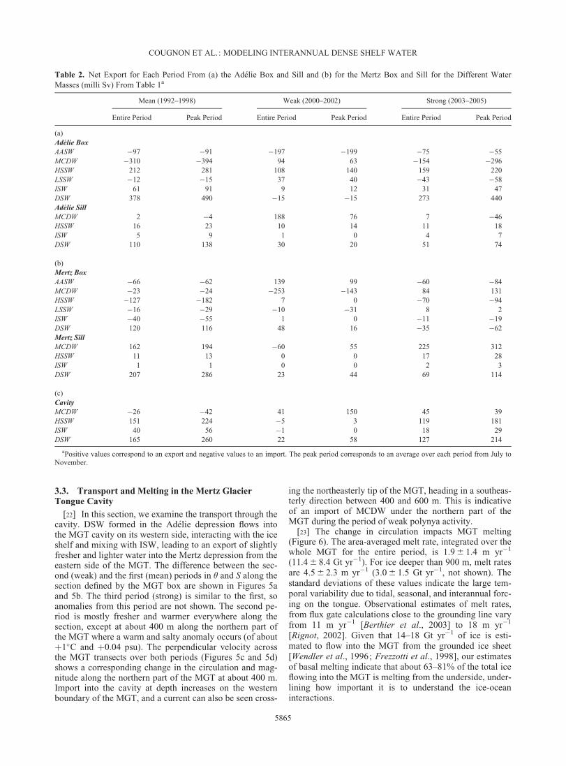
[23] The change in circulation impacts MGT melting(Figure 6). The area-averaged melt rate, integrated over thewhole MGT for the entire period, is 1.9 6 1.4 m yr�1

(11.4 6 8.4 Gt yr�1). For ice deeper than 900 m, melt ratesare 4.5 6 2.3 m yr�1 (3.0 6 1.5 Gt yr�1, not shown). Thestandard deviations of these values indicate the large tem-poral variability due to tidal, seasonal, and interannual forc-ing on the tongue. Observational estimates of melt rates,from flux gate calculations close to the grounding line varyfrom 11 m yr�1 [Berthier et al., 2003] to 18 m yr�1

[Rignot, 2002]. Given that 14–18 Gt yr�1 of ice is esti-mated to flow into the MGT from the grounded ice sheet[Wendler et al., 1996; Frezzotti et al., 1998], our estimatesof basal melting indicate that about 63–81% of the total iceflowing into the MGT is melting from the underside, under-lining how important it is to understand the ice-oceaninteractions.

Table 2. Net Export for Each Period From (a) the Ad�elie Box and Sill and (b) for the Mertz Box and Sill for the Different WaterMasses (milli Sv) From Table 1a

Mean (1992–1998) Weak (2000–2002) Strong (2003–2005)

Entire Period Peak Period Entire Period Peak Period Entire Period Peak Period

(a)Ad�elie BoxAASW �97 �91 �197 �199 �75 �55MCDW �310 �394 94 63 �154 �296HSSW 212 281 108 140 159 220LSSW �12 �15 37 40 �43 �58ISW 61 91 9 12 31 47DSW 378 490 �15 �15 273 440Ad�elie SillMCDW 2 �4 188 76 7 �46HSSW 16 23 10 14 11 18ISW 5 9 1 0 4 7DSW 110 138 30 20 51 74

(b)Mertz BoxAASW �66 �62 139 99 �60 �84MCDW �23 �24 �253 �143 84 131HSSW �127 �182 7 0 �70 �94LSSW �16 �29 �10 �31 8 2ISW �40 �55 1 0 �11 �19DSW 120 116 48 16 �35 �62Mertz SillMCDW 162 194 �60 55 225 312HSSW 11 13 0 0 17 28ISW 1 1 0 0 2 3DSW 207 286 23 44 69 114

(c)CavityMCDW �26 �42 41 150 45 39HSSW 151 224 �5 3 119 181ISW 40 56 �1 0 18 29DSW 165 260 22 58 127 214

aPositive values correspond to an export and negative values to an import. The peak period corresponds to an average over each period from July toNovember.


5865

[24] Figure 6 shows that the period of greatest net melt(3.8 6 1.5 m yr�1) occurs during the second (weak) periodof polynya activity (2000–2002 inclusive) with the maxi-mum melt rate (<8.5 m yr�1) occurring during the summerof 2002/2003. Melting starts to decrease in 2003, corre-sponding to the beginning of the third (strong) period,when the export of dense water increases again. The area-averaged melt rate for the first and the third periods is1.2 6 0.4 m yr�1. Despite the enhanced melting only smallamounts of ISW, defined here as having a potential temper-ature below the freezing temperature at 50 dbar, areexported from beneath the MGT during the second period.This suggests that the additional glacial meltwater iswarmer than our defined freezing temperature, and so is notclassified as ISW and therefore likely to have been pro-duced by warm MCDW during melting.

3.4. Sensitivity of Dense Shelf Water Export to GlacialMeltwater

[25] A recent study by Kusahara and Hasumi [2013] hasshown the importance of including basal melting in model-ing studies such as that one. To test the effect of having iceshelf thermodynamics in our model, a comparison betweenboth the reference simulation and the simulation withoutocean/ice shelf thermodynamics are presented in this sec-tion. Ocean/ice shelf thermodynamics in the model allowsthe formation of fresh and supercooled water due to iceshelf melting, which can mix with the surrounding densewater. Hellmer [2004] has shown that a decrease in ice

shelf area with an associated reduction of basal melting sig-nificantly changes shelf water characteristics and enhancesthe formation of DSW.

[26] Figure 7 shows monthly climatologies of both simu-lations along both sills and along the cavity section on theeastern edge of the MGT. The simulation without ocean/iceshelf thermodynamics shows denser water in the cavity(�0.06 kg m�3 denser) and at both sills (�0.02 kg m�3

denser). Associated with this increased in density, a greatertransport of DSW through these sections is also seen.Around 0.05 Sv more DSW flows from the Ad�elie to Mertzdepression, but over 0.30 Sv extra is exported from theMertz sill. Table 3 summarizes the averaged transportthrough the studied sections.

[27] The simulation without ocean/ice shelf thermody-namic overestimates DSW export by different magnitudesdepending on the region. Compared to the reference simu-lation, DSW export is 100% greater for the Ad�elie sill and50% larger for the entire Ad�elie box. However, for theMertz box, omitting ocean/ice shelf thermodynamics indu-ces an overestimation of DSW export of more than 500%.This very large increase in DSW export through the wholeMertz box is explained by the presence of more ice shelvesin the Mertz box area (MGT, B9b, Ninnis icebergs, andfast ice). This relatively larger ice area in the Mertz depres-sion induces greater volume of fresh and supercooledwater, which mixes with the dense water imported from theAd�elie depression and produced locally, and results inlighter and cooler DSW.

a) b)

c) d)

WEST NORTH EAST

TSEWTSEW

WEST

NORTHNORTH

NORTH

EAST EAST

EAST

Figure 5. Differences in potential (a) temperature and (b) salinity for the MGT box between the second(2000–2002) minus the first (1992–1998) periods. The black line on Figures 5a and 5b shows the MGTice draft for each edge of the ice tongue. (c and d) show the perpendicular velocity through the MGTbox sections for the first and second period respectively (m s�1), with potential density contours. Positivevalues are out of the MGT box.


5866

4. Discussion

4.1. Links Between Polynya Activity, Ice ShelfMelting, and DSW Export

[28] Our results show a delay between the timing of thestrength of polynya activity and the corresponding changein dense water export, not seen in previous studies. Theweaker export, from 2000 to 2002, is delayed by about ayear after the weakest polynya activity occurs during 1999to 2001. The strongest polynya state (2002–2004) inducesan increased DSW export in volume and density steadilyover all three years from 2003 to 2005. However, thisexport remains on average less dense than during the firstperiod (1992–1998). This difference in density exportbetween the two periods suggests that after a period ofweak polynya activity leading to a decrease of DSWexport, three or more years of strong polynya activity areneeded to precondition the density of shelf water to supportthe export of very dense water again. It is interesting tonote that during the ‘‘mean’’ polynya state, there is a stron-ger export of the densest DSW than during the ‘‘strong’’polynya state. This is likely due to the spinup period of themodel. For the 32 spinup years prior to 1992, the modeluses the same forcing (1992–2007), so the water masses at1992 for the ‘‘mean’’ polynya state have been precondi-tioned by the last years of the atmospheric forcing, drivingstronger net export.

[29] The interannual variability in the basal melt rate ofthe MGT follows the same pattern as the DSW export.Whilst the MGT is melting at a rapid rate between 2000and 2002 (3.8 6 1.5 m yr�1), only small amounts of ISWare seen passing through the analysis boxes used in thisstudy. During this time, the glacial meltwater that is pro-duced must mix with the warmer ambient water and form awatermass that contains glacial meltwater which is warmerthan our definition of ISW.

[30] During the weak polynya state, MCDW penetratesfurther on-shelf, although the actual volume entering theAd�elie box does not change significantly from the strong ormean states (2.3 Sv for 1992–1998, 2.1 Sv for 2000–2002,and 2.0 Sv for 2003–2005). The mechanism drivingMCDW onto the shelf may be due to a combination of fac-tors. In some regions, the primary mechanism causingMCDW to move on-shelf is changes in winds [e.g., Steig et

al., 2012; Dinniman et al., 2012]. Alternatively, St-Laurentet al. [2012] demonstrates that a warm slope front currentmay be also guided on-shelf via troughs in the slopebathymetry.

[31] A detailed dynamical examination of the factorsdriving MCDW circulation onto the shelf is beyond thescope of the present study, although qualitatively the MertzBank does appear to be important in guiding intrusions to-ward the MGT (Figure 8). What we find, however, is thatMCDW import is not correlated with changes in DSWexport nor with changes in surface wind stress (not shown).This supports the findings of Marsland et al. [2004] whofound that polynya buoyancy flux was the primary factorcontrolling DSW export and winds had little correlationwith the DSW production. Of course, polynya activity isnot independent from the winds, ocean temperature, or cir-culation and there exist complex feedbacks between thesefactors. However, polynya activity, as measured by heatflux, is representative of an integration of these atmosphericand oceanic terms for the purpose of this study, and we findthat there exists a useful correlation with the strength ofthese polynyas driving DSW export.

[32] The lack of correlation between polynya activityand MCDW import does not imply that inflow from off theshelf is unimportant to the circulation. During weak poly-nya states, the intruding MCDW is not cooled as dramati-cally and may interact with the MGT and modify the iceshelf/ocean driven circulation [Klinck and Dinniman,2010] by intensifying the ice pump mechanism throughcavity enhanced basal melting [Lewis and Perkin, 1986].MCDW driven basal melting makes the water fresher andmore buoyant which causes it to rise along the bottom ofthe ice shelf. This buoyancy driven flow has the effect ofpulling deeper water to the base of the ice shelf. This indu-ces more ice shelf melting which may further decrease theformation and density of DSW in the region. This positivefeedback between intruding warm MCDW and increasedfreshening is discussed further in the following section.

4.2. Regional Circulation

[33] The model allows the detailed examination of DSWexport pathways from the region, and we find several morethan have been previously assumed in observational stud-ies. The time-averaged potential temperature and density at

Net melt rate (m/yr)

Figure 6. Net melt rate from the Mertz Glacier Tongue (in m yr�1), combining the mass lost from the icetongue and the accumulation of frazil ice. Vertical dashed lines show the same polynya transitions as in Figure 3.


5867

the model bottom layer, overlaid with the current directionduring each period is shown in Figure 8. This figure showsthat dense water spreads between both depressions throughthe MGT cavity and over the shelf break. Significant vol-umes of DSW are being exported from the Ad�elie box viathe cavity under the MGT (120 mSv averaged over theentire period) as well as along the coast to the west (fromthe western edge of the Ad�elie box, 18 mSv averaged overthe entire period). The heat flux forcing [Tamura et al.,

2011] includes many small but active polynyas along thecoast to the west of the MGT, such as in CommonwealthBay. The model produces HSSW from these regions duringwinter and transports some DSW westward as part of thecoastal current. However, observations do not find any cir-culation of DSW along the coast, likely because of theirsummertime bias. In the model during summer there is noHSSW production and DSW present in deep troughs anddepressions does not easily escape the shelf region, except

)b)a

)d)c

f )e)

Figure 7. Monthly climatologies averaged over the entire period (1992–2007) for the potential density(left plots) and DSW transport (right plots) for the reference simulation (black line) and the simulationwithout ocean/ice shelf thermodynamics (dashed line) for (a and b) the Ad�elie sill, (c and d) the Mertzsill, and(e and f) the cavity section.


5868

at the Ad�elie sill, as in observations [Williams et al., 2008].Future wintertime observations should observe these watermasses predicted by the model to establish the importanceof export westward via the coastal current and outflows ofthe western edge of the basin.

[34] The off-shelf export is simulated to occur throughboth Ad�elie and Mertz sills and is also identified throughanother region located to the east of the Mertz sill (seeblack circles in Figures 8a and 8b), which export about 32mSv of DSW averaged over the entire period. A significantpart of the export going through the sills is missing in ourcurrent sill section locations. About 51 mSv of DSW, aver-aged over the entire period, is going throughout the westerncorner of the Ad�elie box and about 34 mSv throughout thewestern corner of the Mertz box directly west of the Mertzsill. This highlights the limitations of observational studiesthat only capture narrow regions of transport.

[35] The net export of DSW from the Mertz depressionis greater at the sill than over the entire depression (Table2b) due to the import from the Ad�elie depression via thecavity beneath the MGT. However, the DSW exportedthrough the Mertz sill (with potential temperature between�1.5 and �0.5�C and a salinity below 34.5 psu) has differ-ent properties than the incoming DSW flow from theAd�elie depression (colder than �1.5�C and sometimes salt-ier than 34.5 psu). This suggests that mixing occurs in theMertz depression between DSW coming from the Ad�eliedepression, the DSW or HSSW formed locally due to thepolynya in the lee of B9b iceberg, ISW and overlyingMCDW to produce relatively less dense DSW.

[36] The flow of DSW from the Ad�elie to the Mertzdepression is strongly controlled by the activity of theMGT polynya. Figure 8 and Table 2 show clearly that dur-ing the first period there is significant formation of DSW,occurring mainly in the Ad�elie depression. The DSW cre-ated in the Ad�elie depression flows both into the cavitybeneath the MGT and across the Ad�elie sill toward theabyssal ocean. In contrast, the second (weak) period haswarmer bottom water, particularly over the Mertz depres-

sion and the northern edge of the MGT, and the water issignificantly fresher on the Ad�elie and Mertz banks. Notenough DSW of sufficient volume and density is formed inthe Ad�elie depression to enable the circulation to escapethe shelf at the Ad�elie sill. Some DSW continues to circu-late through the cavity and into the Mertz depression andthrough the sill but at much reduced rate. DSW starts toform again during winter 2003, mainly in the Ad�eliedepression, which then spreads over the shelf to againescape through the Ad�elie sill at lower rate than during thefirst period, indicating a phase lag between the initial for-mation and eventual export of DSW. More than a year ofstrong polynya state is needed to form a sufficient volumeand density of DSW to recover from the weak forcing pe-riod and to flow into the deep ocean.

[37] During the second period a reduced volume of ISWescapes the region, when we may have expected to seemore due to the increased melt rates during this period. Theextra melting is produced by enhanced MCDW penetrationinto the cavity. The warmer water mixes with the melt-water, resulting in a watermass warmer than the definitionof ISW. Our results suggest that the commonly used defini-tion of ISW that we have adopted for this study is inad-equate for quantifying the amount of glacially sourcedmeltwater exported from the shelf.

[38] The additional freshwater produced by the MCDWintrusion and glacial melting may provide one possible ex-planation for the lag between enhanced polynya strengthand the recovery of DSW export following a period ofweak polynya activity. Marsland et al. [2004] showed thatthe volume averaged salinity within the Ad�elie Depressionprior to the onset of winter polynya activity was an impor-tant ‘‘preconditioner’’ for DSW production and more salinepreexisting watermasses led to stronger exports of DSWand vice versa. The enhanced melting of the MGT duringweak polynya states may lead to such preconditioning ofthe water column, from which DSW export subsequentlytakes several years to recover. These dynamics are beyondthe present study, however, and further examination isrequired to establish the impact of the enhanced buoyancyduring weak polynya years.

4.3. Comparison With Other Studies

[39] Two other modeling studies, Marsland et al. [2004]and Kusahara et al. [2011], have examined this area usingglobal domain ocean/sea-ice models, but neither includeimportant ocean/ice shelf/fast-ice interaction processes orthe circulation underneath ice-shelves. Marsland et al.[2004] used the years 1991–2000 to show an interannualvariability in the wintertime heat flux, with weak (1991,1992, 1999–2000) and strong (1993–1998 inclusive) statesin the polynya activity corresponding to different states ofcirculation and magnitudes of DSW export from the region.Kusahara et al. [2011] also examined DSW export fromthe same region. The model was shown to reproduce keywater masses of the region and a seasonal variability in theexport of DSW through the Ad�elie sill linked to the sea-sonal sea-ice production in coastal polynyas area, but didnot include ISW formation.

[40] The export of 100–500 mSv of DSW through theAd�elie Sill observed in 1998 using ADCP moorings[Williams et al., 2008] is substantially higher than the

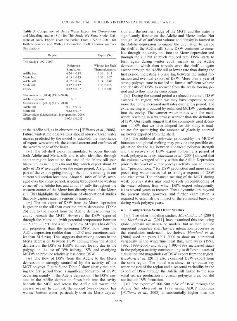
Table 3. Comparison of Dense Water Export for Observationsand Modeling studies (Sv); for This Study We Show Model Esti-mate of DSW Export Over the Period From 1992 to 2007, forBoth Reference and Without Ocean/Ice Shelf ThermodynamicsSimulations

Region Export (Sv)

This Study (1992–2007)ReferenceSimulation

Without Ice ShelfThermodynamics

Ad�elie box 0.24 6 0.18 0.36 6 0.11Mertz box 0.05 6 0.13 0.32 6 0.26Ad�elie sill 0.07 6 0.06 0.14 6 0.07Mertz sill 0.12 6 0.12 0.35 6 0.22Cavity 0.12 6 0.07 0.16 6 0.08

Marsland et al. [2004] (1991–2000)Ad�elie depression 0.15Kusahara et al. [2011] (1979–2008)Ad�elie sill 0.21 6 0.05Mertz sill 0.12 6 0.07Observations (Meijers et al., in preparation, 2008)Ad�elie sill 0.073 6 0.083


5869

modeled value of 70 mSv with the current sill section. Thisdifference may be explained, however, by the assumptionmade by Williams et al. [2008] that the measured currentmagnitude was directed entirely through the Ad�elie sill.This assumption was necessary due to the absence of com-pass heading measurements on the moorings, so the truecurrent direction could not be determined. Subsequentobservations using current meters with compasses measuresubstantially less transport directed through the sill

(73 6 83 mSv), which is in much closer agreement with theresults from our study (Meijers et al., manuscripts inpreparation).

[41] We show a net DSW export of 240 mSv from theAd�elie depression compared to Marsland et al. [2004] whofound 150 mSv. Kusahara et al. [2011] found a strongerexport through the Ad�elie sill (210 mSv) than through theMertz sill (120 mSv), which is the opposite of our patternwith 70 mSv for the Ad�elie sill and 120 mSv for the Mertz

1992 - 1998 1992 - 1998

2000 - 2002 2000 - 2002

2003 - 2005 2003 - 2005

a)

)f)e

b)

c) d)

Figure 8. Potential temperature (left plots) and density (right plots), overlaid with velocity directions(arrows) averaged for each period at the bottom model layer. The velocity field is deduced from stream-lines, but is indicative of direction only. The blue line on the potential temperature plots shows the�0.3�C isotherm, and the red line on the potential density plots is the critical limit for DSW export andAABW formation (1027.88 kg m�3). Dashed lines show box boundaries, black circles show the threemain areas of export, and white lines depth contours.


5870

sill. This difference in sill export is likely due to the circu-lation under the MGT connecting the two depressions,which is not included in either of the previous studies. Bothearlier models consider the MGT as a land barrier separat-ing the two depressions. As the polynyas are stronger in theAd�elie depression area than in the Mertz depression area,Kusahara et al. [2011] therefore shows more DSWexported from the Ad�elie sill than from the Mertz sill. Inour model, the connection between the basins via the MGTcavity enables both the melting of the MGT and the trans-port of DSW from the Ad�elie depression to influence theMertz depression, and thus changes the ratio of DSW thatis exported from each sill. In addition, both Kusahara et al.[2011] and Marsland et al. [2004] cannot produce ISW,which means they may overestimate both the amount anddensity of the DSW, as demonstrated here by the experi-ment where we shut off ocean/ice shelf thermodynamics,which showed that DSW export is up to 100% stronger.

5. Summary

[42] The region near the Mertz Glacier Tongue (MGT) isknown to be a source of Dense Shelf Water (DSW) that con-tributes to the formation of Antarctic Bottom Water(AABW) [Rintoul, 1998; Marsland et al., 2004; Williams etal., 2008; Kusahara et al., 2011] and is associated withintense polynya activity. Here we have used a regional iceshelf/ocean model to investigate the shelf sea processes con-trolling the export of DSW from the continental shelf in thevicinity of the MGT. The model is improved over previousstudies in that it includes ice shelf/ocean interaction proc-esses, and a cavity beneath the MGT linking the two majorregional shelf depressions. Modeled DSW export is in goodagreement with available, although sparse, observations.

[43] Here we show that there is a delay of about a yearbetween the change of polynya activity and the DSWexport response. A single year of significantly weaker poly-nya activity can limit DSW export. A prolonged strong ormean polynya state (>1 year) is, however, needed for thevolume of DSW on the continental shelf and depression tobecome large enough to escape the sill and move downslope to the abyssal ocean. We note, as previous studieshave already done [Williams et al., 2010], that using a fixedcritical density to define DSW is limiting and does notalways capture the true export of DSW to the abyssalocean. The critical value required for DSW to flow off-shelf should instead depend on the relative difference in theon-shelf DSW and the ambient off-shore water densitiesfor greater accuracy.

[44] The connection between basins under the MGTallows dense water (mainly High Salinity ShelfWater—HSSW) from the Ad�elie depression to enter theMertz depression as well as contributing to ice shelf basalmelt. The glacial meltwater produced further decreases thedensity of DSW, and limits the net export of DSW. Wehighlight that models without ocean/ice shelf interactionprocesses will significantly overestimate rates of DSW andAABW export. We also show that in addition to the Ad�elieand Mertz sills DSW can also flow out of the continentalshelf through the north eastern edge of the Mertz depres-sion, and along the coast to the west of the Ad�elie depres-

sion, although whether or not these pathways contribute toAABW formation is unknown.

[45] Our study shows that DSW formed from active pol-ynyas plays an important role in insulating ice shelves frommelting by intrusions of relatively warm Modified Circum-polar Deep Water (MCDW). Here, our results suggest thatduring a sustained decrease in DSW formation, due to areduction in the strength of the polynya activity (reductionin the strength of brine rejection), warm and salty MCDWwill flow further on-shelf and drive higher ice shelf basalmelting. The strong coupling between the polynya activity,DSW export and the basal melting of the MGT highlightsthe importance of understanding atmosphere-ocean-iceshelf interaction processes over the continental shelf seas,as well as exchange of water across the shelf break.

[46] We show that high interannual subglacial meltingand the coupling between the polynya activity, the variabil-ity of the volume and the density of DSW and glacial melt-water is likely to be an important control on AABWvariability. Unfortunately, the lack of long-term bottomwater observations does not presently allow the evaluationof the interannual variability study in terms of DSW exportand in terms of quantifying the AABW freshening due toatmospheric forcing.

[47] Acknowledgments. This work was supported by the AustralianGovernment’s Cooperative Research Centres Program through the Antarc-tic Climate & Ecosystems Cooperative Research Centre (ACE CRC) andby CNRS through the Laboratoire d’Etude en G�eophysique etOc�eanographie Spatiale (LEGOS), France and the CRACICE project.Computing hours were provided by both the Tasmanian Partnership forAdvanced Computing and the Australian National Computing Infrastruc-ture under grant m68. The ROMS code was kindly provided by TheROMS/TOMS Group under the MIT/X License. We thank Simon Mars-land (CSIRO, Australia) and Steve Rintoul (CSIRO, Australia), for helpfuldiscussions during the development of the simulation. We also thank LarsSmedsrud (Geophysical Institute, University of Bergen), Scott Springer(Earth & Space Research, Seattle), and an anonymous reviewer for theirconstructive comments on the manuscript during the reviewing process.

ReferencesAoki, S., S. R. Rintoul, S. Ushio, and S. Watanabe (2005), Freshening of

the Ad�elie land bottom water near 140oE, Geophys. Res. Lett., 32,L23601, doi:1029/2005GL024246.

Beaman, R. J., P. E. O’Brien, A. L. Post, and L. D. Santis (2011), A newhigh-resolution bathymetry model for the Terre Ad�elie and the George Vcontinental margin, East Antarctica, Antarct. Sci., 23, 95–103,doi:10.1017/S095410201000074X.

Berthier, E., B. Raup, and T. Scambos (2003), New velocity map and mass-balance estimate of Mertz glacier, East Antarctica, derived from landsatsequential imagery, J. Glaciol., 49, 503–511.

Bindoff, N. L., S. R. Rintoul, and R. Massom (2000), Bottom water forma-tion and polynyas in Adelie Land, Antarctica, Pap. Proc. R. Soc. Tasma-nia, 133(3), 51–56.

Bindoff, N. L., G. D. Williams, and I. Allison (2001), Sea-ice growth andwater mass modification in the Mertz Glacier polynya, East Antarctica,during winter, Ann. Glaciol., 33, 399–406.

Cottin, J., B. Raymond, A. Kato, F. Am�elineau, Y. L. Maho, T. Raclot, B.Galton-Fenzi, A. Meijers, and Y. Ropert-Coudert (2012), Foraging strat-egies of male Ad�elie penguins during their first incubation trip in relationto environmental conditions, Mar. Biol., 159(8), 1843–1852,doi:10.1007/s00227-012-1974-x.

Dinniman, M., J. Klinck, and E. Hofmann (2012), Sensitivity of Circumpo-lar Deep Water transport and ice shelf basal melt along the west Antarc-tic Peninsula to changes in wind, J. Clim., 25(14), 4799–4816,doi:10.1175/JCLI-D-11–00307.1.

Dinniman, M. S., J. M. Klinck, and W. O. Smith Jr. (2003), Cross-shelfexchange in a model of the Ross Sea circulation and biogeochemistry,Deep Sea Res., Part II, 50, 3103–3120.


5871

Dinniman, M. S., J. M. Klinck, and W. O. Smith Jr. (2007), Influence of seaice cover and icebergs on circulation and water mass formation in a nu-merical circulation model of the Ross Sea, Antarctica, J. Geophys. Res.,112, C11013, doi:10.1029/2006JC004036.

Fraser, A. D., R. A. Massom, K. J. Michael, B. K. Galton-Fenzi, and J. L.Lieser (2012), East Antarctic landfast sea ice distribution and variability,2000–08, J. Clim., 25(4), 1137–1156.

Frezzotti, M., A. Cimbelli, and J. Ferrigno (1998), Ice-front change and ice-berg behaviour along Oates and George V coasts, Antarctica, 1912–96,Ann. Glaciol., 27(167), 643–650.

Fukamachi, Y., K. I. Ohshima, S. Aoki, Y. Kitade, T. Tamura, and M.Wakatsuchi (2010), Antarctic Bottom Water revealed by mooring meas-urements off Cape Darnley, Antarctica, in International Polar Year OsloScience Conference, Oslo, Norway, 8–12 Jun.

Galton-Fenzi, B. K. (2009), Modelling ice-shelf/ocean interaction, PhDthesis, Univ. of Tasmania, Hobart, Tasmania.

Galton-Fenzi, B. K. (2010), Modelling the interaction between Antarcticaand the Southern Ocean, Tech. Rep. 33, edited by A. J. Hollis and K. A.Day, Cent. for Aust. Weather and Clim. Res. Tech. Rep.

Galton-Fenzi, B. K., J. R. Hunter, R. Coleman, S. J. Marsland, and R.Warner (2012), Numerical modelling of melt/freeze beneath the AmeryIce Shelf, J. Geophys. Res., 117, C09031, doi:10.1029/2012JC008214.

Greenbaum, J. S., D. D. Blankenship, D. A. Young, T. G. Richter, B.Legr�esy, B. Galton-Fenzi, and Y. Gim (2010), Basal characteristics andinferred bathymetry beneath the Mertz Glacier Tongue, Antarctica, fromcoupled airborne radar sounding and gravity prior to the February 12th2010 breakup event, in 4th SCAR Open Science Conference—Antarctica:Witness to the Past and Guide to the Future, 3–6 Aug., Buenos Aires.

Griffies, S., et al. (2009), Coordinate Ocean-ice reference experiment(COREs), Ocean Modell., 26, 1–46.

Hasumi, H. (2006), Ocean Component Model (COCO) version 4.0, CCSRRep. 25, Cent. for Clim. Syst. Res., Univ. of Tokyo.

Hellmer, H. H. (2004), Impact of Antarctic ice shelf basal melting on seaice and deep ocean properties, Geophys. Res. Lett., 31, L10307,doi:10.1029/2004GL019506.

Hemery, L. G., B. K. Galton-Fenzi, N. Am�eziane, M. J. Riddle, S. R. Rin-toul, R. J. Beaman, A. L. Post, and M. El�eaume (2011), Predicting habi-tat preferences for Anthometrina adriani (Echinodermata) on the EastAntarctic continental shelf, Mar. Ecol. Prog. Ser., 441, 105–116,doi:10.3354/meps09330.

Holland, D. M., and A. Jenkins (1999), Modelling thermodynamic iceocean interactions at the base of an ice shelf, J. Phys. Oceanogr., 29,1787–1800.

Jacobs, S. S. (2004), Bottom water production and its link with the thermo-haline circulation, Antarct. Sci., 16(4), 427–437.

Kanamitsu, M., W. Ebisuzaki, J. Woollen, S.-K. Yang, J. Hnilo, M. Fiorino,and G. Potter (2002), Ncep-doe amip-ii reanalysis (r-2), Bull. Am. Mete-orol. Soc., 83(11), 1631–1643.

Klinck, J. M., and M. S. Dinniman (2010), Exchange across the shelf break at highsouthern latitudes, Ocean Sci., 6(2), 513–524, doi:10.5194/os-6-513-2010.

Kusahara, K., and H. Hasumi (2013), Modeling Antarctic ice shelfresponses to future climate changes and impacts on the ocean, J. Geo-phys. Res. Oceans, 118, 2454–2475, doi:10.1002/jgrc.20166.

Kusahara, K., H. Hasumi, and T. Tamura (2010), Modeling sea ice produc-tion and dense shelf water formation in coastal polynyas around EastAntarctica, J. Geophys. Res., 115, C10006, doi:10.1029/2010JC006133.

Kusahara, K., H. Hasumi, and G. D. Williams (2011), Dense shelf waterformation and brine-driven circulation in the Ad�elie and George V Landregion, Ocean Modell., 37, 122–138.

Large, W. G., and S. G. Yeager (2009), The global climatology of an inter-annually air-sea flux data set, Clim. Dyn., 33, 341–364.

Legr�esy, B., A. Wendt, I. Tabacco, F. R�emy, and R. Dietrich (2004), Influ-ence of tides and tidal current on Mertz Glacier, Antarctica, J. Glaciol.,50(170), 427–435.

Lewis, E. L., and R. G. Perkin (1986), Ice pumps and their rates, J. Geo-phys. Res., 91(C10), 11,756–11,762.

Marsland, S. J., N. L. Bindoff, G. D. Williams, and W. F. Budd (2004),Modeling water mass formation in the Mertz Glacier Polynya and AdelieDepression, East Antarctica, J. Geophys. Res. 109, C11003,doi:10.1029/2004JC002441.

Marsland, S. J., H. Haak, J. H. Jungclaus, M. Latif, and F. Röske (2007),Antarctic coastal polynya response to climate change, J. Geophys. Res.,112, C07009, doi:10.1029/2005JC003291.

Massom, R. A., K. L. Hill, V. I. Lytle, A. P. Worby, M. J. Paget, and I. Alli-son (2001), Effects of regional fast-ice and iceberg distributions on thebehaviour of the Mertz Glacier polynya, East Antarctica, Ann. Glaciol.,33, 391–398.

Massom, R. A., K. Hill, C. Barbraud, N. Adams, A. Ancel, L. Emmerson,and M. J. Pook (2009), Fast ice distribution in A�elie Land, East Antarc-tica: inter annual variability and implications for emperor penguinsAptenodytes forsteri, Mar. Ecol. Prog. Ser., 374, 243–257.

Massom, R. A., A. B. Giles, H. A. Fricker, R. C. Warner, B. Legr�esy, G.Hyland, N. Young, and A. D. Fraser (2010), Examining the interactionbetween multi-year landfast sea ice and the Mertz Glacier Tongue, EastAntarctica: Another factor in ice sheet stability?, J. Geophys. Res., 115,C12027, doi:10.1029/2009JC006083.

Mayet, C., L. Testut, B. Legresy, L. Lescarmontier, and F. Lyard (2013),High resolution barotropic modeling and the calving of the Mertz Glacier,East Antarctica, J. Geophys. Res. Oceans, 118, doi:10.1002/jgrc.20166.

Menemenlis, D., J. M. Campin, P. Heimbach, C. Hill, T. Lee, A. Nguyen,M. Schodlock, and H. Zhang (2008), ECCO2: High resolution globalocean and sea ice data synthesis, Mercator Ocean Q. Newsl., 31, 13–21.

Mueller, R. D., L. Padman, M. S. Dinniman, S. Y. Erofeeva, H. A. Fricker,and M. A. King (2012), Impact of tide-topography interactions on basalmelting of Larsen C Ice Shelf, Antarctica, J. Geophys. Res., 117,C05005, doi:10.1029/2011JC007263.

Ohshima, K. I., et al. (2013), Antarctic Bottom Water production byintense sea-ice formation in the Cape Darnley polynya, Nat. Geosci., 6,235–240.

Orsi, A. H., G. C. Johnston, and J. B. Bullister (1999), Circulation, mixingand production of Antarctic Bottom Water, Prog. Oceanogr., 43(1), 55–109.

Rignot, E. (2002), Mass balance of East Antarctic glaciers and ice shelvesfrom satellite data, Ann. Glaciol., 34(1), 217–227.

Rintoul, S. (1998), On the origin and influence of Ad�elie Land BottomWater, in Ocean, Ice, and Atmosphere: Interaction at the Antarctic Con-tinental Margin, Antarct. Res. Ser., vol. 75, edited by S. Jacobs and R.Weiss, pp. 151–172, AGU, Washington, D. C.

Rintoul, S. (2007), Rapid freshening of Antarctic Bottom Water formed inthe Indian and Pacific oceans, Geophys. Res. Lett., 34, L06606,doi:10.1029/2006GL028550.

Shchepetkin, A. F., and J. C. McWilliams (2005), The Regional OceanicModeling system (ROMS): A split-explicit, free-surface, topography-following-coordinate oceanic model, Ocean Modell., 9, 347–404,doi:10.1016/j.ocemod.2004.08.002.

St-Laurent, P., J. M. Klinck, and M. S. Dinniman (2012), On the role ofcoastal troughs in the circulation of warm circumpolar deep water onAntarctic shelves, J. Phys. Oceanogr., 43, 51–64.

Steig, E. J., Q. Ding, D. S. Battisti, and A. Jenkins (2012), Tropical forcingof Circumpolar Deep Water Inflow and outlet glacier thinning in theAmundsen Sea Embayment, West Antarctica, J. Glaciol. 53(60), 19–28,doi:10.3189/2012AoG60A110.

Tamura, T., K. I. Ohshima, and S. Nihashi (2008), Mapping of sea ice pro-duction for Antarctic coastal polynyas, Geophys. Res. Lett., 35, L07606,doi:10.1029/2007GL032903.

Tamura, T., K. I. Ohshima, S. Nihashi, and H. Hasumi (2011), Estimationof surface heat/salt fluxes associated with sea ice growth/melt in theSouthern Ocean, SOLA, 7(0), 17–20.

Timmermann, R. et al. (2010), A consistent dataset of Antarctic ice sheettopography, cavity geometry, and global bathymetry, Earth Syst. Sci.Data, 3, 231–257.

Wendler, G., K. Ahlna, and C. S. Lingle (1996), On Mertz and Ninnis gla-ciers, East Antarctica, J. Glaciol., 42(142), 447–453.

Williams, G. D., and N. L. Bindoff (2003), Wintertime oceanography ofthe Ad�elie Depression, Deep Sea Res., Part II, 50, 1373–1392.

Williams, G. D., N. L. Bindoff, S. J. Marsland, and S. R. Rintoul (2008),Formation and export of dense shelf water from the Ad�elie Depression,East Antarctica, J. Geophys. Res., 113, 4039, doi:10.1029/2007JC004346.

Williams, G. D., S. Aoki, S. S. Jacobs, S. R. Rintoul, T. Tamura, and N. L.Bindoff (2010), Antarctic Bottom Water from the Ad�elie and George VLand coast, East Antarctica (140–149�E), J. Geophys. Res. 115, C04027,doi:10.1029/2009JC005812.

Wunsch, C., P. Heimbach, R. Ponte, I. Fukumori, and the ECCO-GODAE Consortium Members (2009), The global general circulationof the ocean estimated by the ECCO Consortium, Oceanography,22(2), 88–103.


5872

Documents

Modeling interannual dense shelf water export in the ...klinck/Reprints/PDF/cougnonJGR2013.pdf · Modeling interannual dense shelf water export in the region of the Mertz Glacier