Modeling deposit prices

G U S T A V W A L Å S

Master of Science Thesis Stockholm, Sweden 2013

Modeling deposit prices

G u s t a v W a l å s

Degree Project in Mathematical Statistics (30 ECTS credits) Degree Programme in Engineering Physics (270 credits)

Royal Institute of Technology year 2013 Supervisor at KTH was Boualem Djehiche

Examiner was Boualem Djehiche

TRITA-MAT-E 2013:20 ISRN-KTH/MAT/E--13/20--SE Royal Institute of Technology School of Engineering Sciences KTH SCI SE-100 44 Stockholm, Sweden URL: www.kth.se/sci

Modeling deposit prices

Gustav Walas

May 17, 2013

Abstract

This report investigates whether there are sufficient differences between a bank’sdepositors to motivate price discrimination. This is done by looking at time series ofindividual depositors to try to find predictors by a regression analysis. To be able toconclude on the value of more stable deposits for the bank and hence deduce a price,one also needs to look at regulatory aspects of deposits and different depositors.Once these qualities of a deposit have been assigned by both the bank and regulator,they need to be transformed into a price. This is done by replication with marketfunding instruments.

1

Contents

1 Introduction 3

2 Delimitations 3

3 Background 43.1 A basic deposit pricing method . . . . . . . . . . . . . . . . . . . . . . . . 43.2 Funds transfer pricing and its impact on deposit pricing . . . . . . . . . . 43.3 Academic research on deposit pricing . . . . . . . . . . . . . . . . . . . . . 93.4 Commercial deposit modeling . . . . . . . . . . . . . . . . . . . . . . . . . 93.5 Legislation and regulations . . . . . . . . . . . . . . . . . . . . . . . . . . 11

4 Regression analysis of the depositor base 144.1 Data selection . . . . . . . . . . . . . . . . . . . . . . . . . . . . . . . . . . 144.2 Product characteristics . . . . . . . . . . . . . . . . . . . . . . . . . . . . . 154.3 Assessing deposit stability . . . . . . . . . . . . . . . . . . . . . . . . . . . 154.4 Regression results . . . . . . . . . . . . . . . . . . . . . . . . . . . . . . . . 15

5 What is the tenor of a deposit? 195.1 Relating deposits to other funding sources . . . . . . . . . . . . . . . . . . 195.2 The set of Market Instruments . . . . . . . . . . . . . . . . . . . . . . . . 205.3 Prizing through replication . . . . . . . . . . . . . . . . . . . . . . . . . . 21

6 Discussion 24

7 Biography 25

2

1 Introduction

Deposits are important to banks as funding but also to maintain relationships by havinga complete and competitive offer. As such there are many different aspects when pricingdeposits. The focus of this report will however be to develop a pricing model to beable to assess the value of deposits for the bank as a source of funding in complementto bonds, equity and other financial instruments and only briefly describe some of thefactors that are likely to affect the interest rate paid to the depositor.

Deposits are in this context defined as money placed into a banking institution forsafekeeping overnight or at term. The deposit can be made either on savings accounts,checking accounts or money market accounts. Withdrawal of deposits on accounts mightbe subject to conditions while money market deposits most often have a fixed tenor.

The value of a deposit is ultimately dependent on its stability or likelihood of notbeing withdrawn. The simple logic is that the longer time it will remain in the bank thelonger time the bank can lend out that money and, as a long loan is worth more thana short one, charge a higher price for it. As all deposits have a contractual tenor thiscould be used for pricing but as behavior might be very different from what is allowedby the contractual terms the value is poorly represented by the contractual tenor.

Apart from the stability of the deposit, regulatory aspects of liquidity risk also havepricing implications. The Basel Committee on Banking Supervision has put forwardrecommendations on how liquidity risk can be regulated. This has not yet been imple-mented on European level but the Swedish Financial Supervisory Authority (SwFSA)has implemented a quantitative metric on liquidity risk which was put into place start-ing from January 1, 2013. It is expected that a different but very likely similar metricwill be implemented in the European Union by January 1, 2015. In this propositionthe stability of deposits has been assessed and hence this gives a view of the value ofdeposits in general.

2 Delimitations

This study will try to establish the value of deposits as a funding source for the bank.This means that the results presented in this model constitute a suggestion of whatthe bank’s treasury function should be willing to pay for deposits given the currentalternative. This rate does not necessarily compare to the interest rate received by adepositor as the deposit might be priced stand alone and then has to generate incomethrough a margin or as part of an offering where margins might be negative on thisspecific product. Much of the research on the dynamics of deposit prices relates to thepaid rates, which only to a certain degree represents the value of the deposit as a fundingsource.

3

3 Background

In this section we will go through a wide range of aspects that need to be consideredwhen assessing the value of a deposit. Even though most articles on deposits focus onpricing on the dynamics of retail deposit rates this is interesting as there are no clearcuts in segmentation of deposits and depositors

3.1 A basic deposit pricing method

As previously said the contractual tenors of deposits do not fully reflect the value butone can derive a least favorable valuation since the contractual duration of the deposittells us that it will remain at least that long in the bank. The value as a function of thecontractual tenor can be found by looking at observable market rates as the differentIBOR rates which reflects the banks funding costs for different tenors. For tenors longerthan a year one can look at senior unsecured bond prices to deduct an appropriateinterest rate. This way of looking at deposits underestimates the values of depositswhere behavioral tenors are much longer than contractual ones but it reflects the valueof deposits in the case where we does not allow any assumptions of prolongation andmay serve as a reference point to any other derived value.

3.2 Funds transfer pricing and its impact on deposit pricing

The value of a deposit for a bank is dependent on what return the bank can get fromlending the amount received. So to be able to know whether or not to accept a deposit weneed some reference rate reflecting lending or investment opportunities. Banks typicallyhave a funds transfer price (FTP) framework from which margins on deposits and lendingcan be calculated. A very simple way of calculating a fund transfer price is to calculatea weighted average cost of capital (WACC) which then can serve as a reference forcalculating margins on lending or specific funding sources.

Dermine (2011) brings up several aspects of setting FTPs by creating a foundationand an advanced FTP framework. The foundation approach (named FTP1) uses threecomponents, the price elasticity of loans and deposits with regards to the banks cus-tomers and an interbank rate (IBOR). Under the assumption that the interbank marketis sufficiently deep to not react to any additional lending or deposits from one singlebank the situation can be represented as in figure 1.

Here lending and borrowing decisions are independent of each other but only dependon the IBOR rate and hence the name separation theorem. Optimal lending and depositvolumes can be derived as LOPT and DOPT while the gap or surplus can be covered ordeposited in the interbank market. Figure 1 represents a specific tenor e.g. a two yearterm loan. One would have to apply the same methodology for all tenors that are ofinterest to the bank.

For products where contractual and behavioral tenor is very different e.g. depositson salary accounts or savings accounts without conditions Dermine (2011) suggests amulti period approach (FTP2). For this purpose the deposit volume is split into core

4

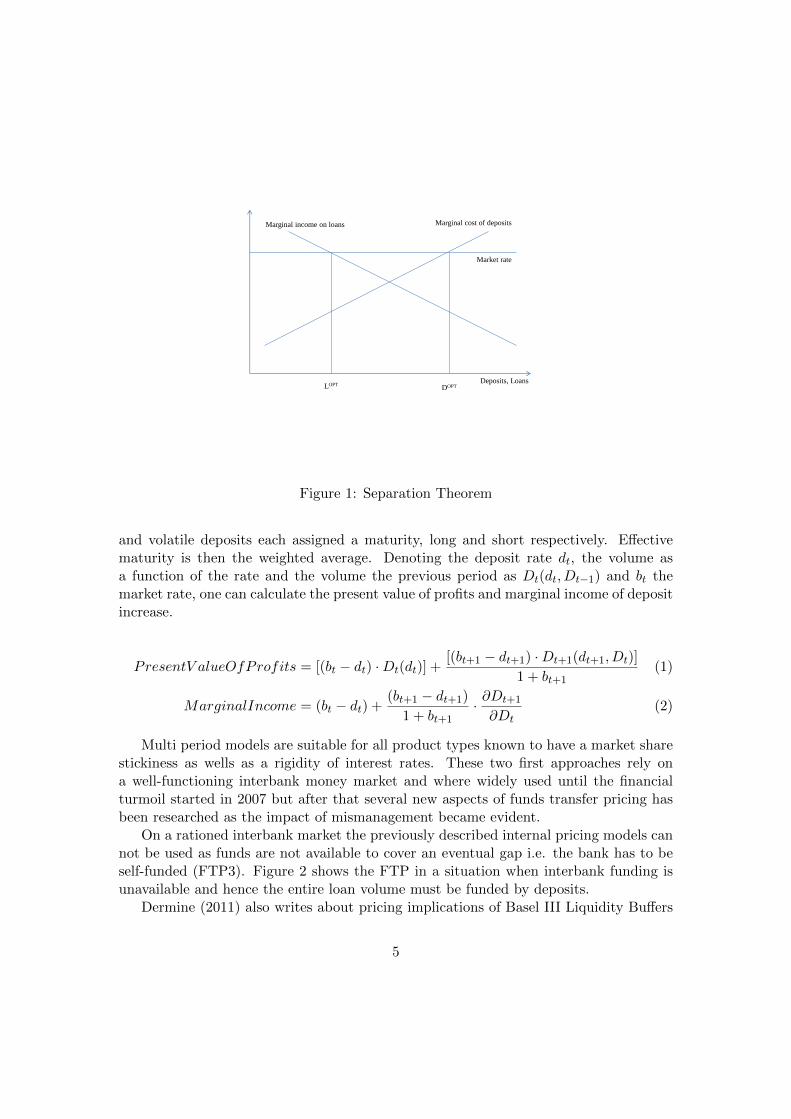
Deposits, Loans

Marginal cost of deposits Marginal income on loans

Market rate

DOPT LOPT

Figure 1: Separation Theorem

and volatile deposits each assigned a maturity, long and short respectively. Effectivematurity is then the weighted average. Denoting the deposit rate dt, the volume asa function of the rate and the volume the previous period as Dt(dt, Dt−1) and bt themarket rate, one can calculate the present value of profits and marginal income of depositincrease.

PresentV alueOfProfits = [(bt − dt) ·Dt(dt)] +[(bt+1 − dt+1) ·Dt+1(dt+1, Dt)]

1 + bt+1(1)

MarginalIncome = (bt − dt) +(bt+1 − dt+1)

1 + bt+1· ∂Dt+1

∂Dt(2)

Multi period models are suitable for all product types known to have a market sharestickiness as wells as a rigidity of interest rates. These two first approaches rely ona well-functioning interbank money market and where widely used until the financialturmoil started in 2007 but after that several new aspects of funds transfer pricing hasbeen researched as the impact of mismanagement became evident.

On a rationed interbank market the previously described internal pricing models cannot be used as funds are not available to cover an eventual gap i.e. the bank has to beself-funded (FTP3). Figure 2 shows the FTP in a situation when interbank funding isunavailable and hence the entire loan volume must be funded by deposits.

Dermine (2011) also writes about pricing implications of Basel III Liquidity Buffers

5

Deposits, Loans

Marginal cost of deposits Marginal income on loans

Market rate

DOPT LOPT

FTP Rate

Figure 2: Separation Theorem on Rationed Interbank Market

which impact mainly the usage of demand deposits for funding loans. This approach isbased on a five component balance sheet found in table 1.

Table 1: Simplified balance sheet

Assets Liabilities

Loans L Deposits DInterbank Deposits I (i)

Liquid Bonds B (b) Long Term Debt F (f)

Under the condition that the entire buffer is funded by long term funding, α % ofdeposits has to be covered by reserve and β % of interbank funding has to be covered bythe reserve. The result is that the marginal cost of loans and deposits has to be adjustedwith the cost or revenue related to the liquidity reserve. This can be described by thefollowing expressions called FTP4.

MarginalCostOfLoans = i+ [β ∗ (f − b)] (3)

MarginalIncomeOfDeposits = i+ [(β − α) ∗ (f − b)] (4)

Asset quality should impact the bank’s funding cost and hence the cost of liquiditymirrored by the FTP. Taking an example with an A rated bank with a funding cost

6

of 5,6% and a cost of equity of 10% buying a AAA rated asset expected to yield 5,5%while the market expects 5%. With a tax of 40% on profits the Economic profit can becalculated as follows.

StandardEconomicProfit = Profit− CostOfAllocatedEquity= (1− 0, 4) ∗ [5, 5% ∗ 100− 5, 6% ∗ 98]− [10% ∗ 2] = −0, 1928 (5)

The standard economic profit is likely to be underestimated since the value createdby the safe loan is charged a too high cost of interbank debt and equity. The very safeAAA asset reduces the overall risk of the debt of the bank and hence the marginal costof interbank funding should be less than 5,6% and the same goes for cost of equity. Arevised method to calculate the economic profit can be derived by looking at the twobalance sheets in tables 2 and 3. Table 2 represents a typical leveraged bank balancesheet and while table 3 represents an unleveraged transaction for the bank but with afunding transaction on behalf of the shareholders.

Table 2: Traditional balance sheet

Assets Liabilities

New Safe Loan 100 (5,5%) Debt 98Equity 2

Table 3: Revised balance sheet

Assets Liabilities

New Safe Loan 100 (5,5%) Equity 100 (5%)-Debt 98 (5%-ε) -Equity 98 (5%-ε)

Calculating the economic profit with a demanded return on equity of 5% as expectedby the markets and a funding cost ε smaller than 5% since there is an equity cushionprotecting the lenders Dermine (2011) finds the following advanced economic profit ofbuying the asset.

AdvancedEconomicProfit = (P/L− CostOfAllocatedEquity)bond

+ (P/L− CostOfAllocatedEquity)funding

= [(1− 0, 4) ∗ 5, 5% ∗ 100− 5% ∗ 100]

+ [−(1− 0, 4) ∗ (5%− ε) ∗ 98− (5%− ε) ∗ 98]

≈ 0, 26 (6)

This result indicates that the transaction should be done with regard to the economicprofit of the shareholders. The ability to differentiate the funding costs with regard to

7

asset quality as presented in FTP5 changed the view of whether the deal would beprofitable or not.

Dermine (2011) also discusses the implications of Basel III metrics such as the NetStable Funding Ratio which compares asset and liability mismatch around the 1 Yearpoint and concludes that the relevant funds transfer price in such an environment willbe the market rate on the banks long term debt (FTP6).

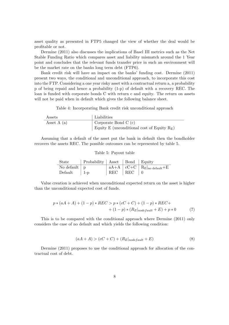
Bank credit risk will have an impact on the banks’ funding cost. Dermine (2011)present two ways, the conditional and unconditional approach, to incorporate this costinto the FTP. Considering a one year risky asset with a contractual return a, a probabilityp of being repaid and hence a probability (1-p) of default with a recovery REC. Theloan is funded with corporate bonds C with return c and equity. The return on assetswill not be paid when in default which gives the following balance sheet.

Table 4: Incorporating Bank credit risk unconditional approach

Assets Liabilities

Asset A (a) Corporate Bond C (c)Equity E (unconditional cost of Equity RE)

Assuming that a default of the asset put the bank in default then the bondholderrecovers the assets REC. The possible outcomes can be represented by table 5.

Table 5: Payout table

State Probability Asset Bond Equity

No default p aA+A cC+C RE|no default+EDefault 1-p REC REC 0

Value creation is achieved when unconditional expected return on the asset is higherthan the unconditional expected cost of funds.

p ∗ (aA+A) + (1− p) ∗REC > p ∗ (cC + C) + (1− p) ∗REC+

+ (1− p) ∗ (RE |nodefault + E) + p ∗ 0 (7)

This is to be compared with the conditional approach where Dermine (2011) onlyconsiders the case of no default and which yields the following condition:

(aA+A) > (cC + C) + (RE |nodefault + E) (8)

Dermine (2011) proposes to use the conditional approach for allocation of the con-tractual cost of debt.

8

3.3 Academic research on deposit pricing

In the article ”Using physical models to describe and vale core deposits” a model is devel-oped that ”link rate policy to rate modeling”, ”provide a basis for interpreting modelingparameters” and ” propose a conceptual foundation for valuing retail deposits, includingcore deposits”. The retail market is characterized by its size (US bank retail depositstotals more than $3.0 trillion) and its illiquidity (about 1 % turnover). Hence with agood pricing strategy one can build a large low-cost funding base. Building a model forpricing deposits is complex due to the large extent of optionality surrounding depositscompared to other financial derivatives. These options consists of a continuous bankoption to increase maintain and decrease rates, continuous customer option to withdrawpartial or entire balances and continuous customer option to increase balances. In itsturn, rate setting might be affected by ”customer perception of implicit product specificfloors”, ”bank perception of product-specific caps”, ”increased availability of customeralternatives”, which increase the probability of customers exercising their balance with-drawal option. The rate to be assumed driving change in bank deposit rates is supposedto be LIBOR and hence the model uses three-months LIBOR. Banks have in practiceused their optionality to change rates as follows; moving deposit rates in same directionas market rates, changing deposit rates less (or more) than the change in market rates(for example, fractional sensitivity) and changing retail rates at a later date than thechange in wholesale rates (for example, lagging behaviors). The authors state three fun-damental postulates; for every market rate there is a unique equilibrium rate and viceversa, equilibrium response is achieved only after the passage of sufficient time and themarket-administered rate relationship is linear. The postulates are identical to assump-tions of relaxation processes in condensed-matter physics and hence implies that similarmodels might be used for setting interest rates. This gives the possibility of constructinga model not solely based on regressions but derived from a set of theoretically consistentrelationships long established in literature. Market rate, deposit service cost competitiveresponses, yield curve slope measures and macroeconomic factors are stressors likely toaffect the deposit rate. Fitting data to the models reveals that money market and timedeposit rates exhibit similar behavior but deposit rates are quicker to follow market ratesby a factor three. When reviewing bank and regulatory valuation of core deposits thearticle concludes that bank practitioners typically value bank deposits by explicit cashflow definitions.

3.4 Commercial deposit modeling

Firmac Solutions has a service/solution that they call ”Deposit Analytics - a predic-tive solution for deposit pricing and management”. In the article ”Deposit pricing andmanagement through price optimization and predictive behavioral modeling” they statethat methods for deposit pricing are rather unsophisticated. The most commonly usedtechnique seems to be checking the competition and pricing accordingly. This is said tobe efficient only if all organizations operate with equal efficiencies and that the depos-itors of each institution possess the same price sensitivities. Other techniques judged

9

to be mundane by Firmac Solutions are ””walking rates”, simple account segmentationor sectoring, establishing pricing ”rules”, pricing at the margin and monitoring to see ifthings are working...”. Walking rates refer to raising prices until desired balance growthis reached. Firmac solutions believe that deposit pricing should have a methodologyfrom a mathematical perspective, be able to predict balances and depositor behavior,measure net cost of a deposit at a given offered price level, determine net present valueof a deposit gained and should address efficiency of deposit gathering. Firmac’s methodis based on ”seeking an equilibrium rate that is in response to changes in market rate.With factors bearing such elasticities (both short and long term), future market rates,competitor pricing responses, account migration, cannibalization...”.1 Essential to getgood results is to understand the behavior of all depositors but one must also see the”larger context of asset and liability management (ALM) with issues such as liquidityneeds, slope of the curve, duration matching, alternative cost of funds, and others”.2

The model developed by Fimac is for price optimization and does not give any supportto the more strategic ALM questions.

Novantas Solutions supplies a tool called Pricetek to be used for deposit pricing.The tool is said to be able to earn an additional 10 to 15 bps compared to a nonprice discriminating strategy. Parameters used for analyzing deposit market includescompetitor characteristics, rate history, projection of future market rates based on pastcorrelation to indexes and the yield curve.

Deposit prices are impacted by market structures and several studies have been car-ried out to find explanatory factor to interest rate levels. One of the most studied factorsis market concentration. Typically a high degree of concentration leads to lower interestrates on deposits. Size and structure of the banks on the market may also impact theprices i.e. large banks might have a wider range of investment and funding opportuni-ties than smaller banks. The direction of this impact remains somewhat unclear. Largebanks should be able to pay up more for deposits as they should have a larger range ofinvestment opportunities but on the other hand might be able to have a more oppor-tunistic approach to a certain depositor segment as they have a wider range of fundingsources. Another possible reason for small and large banks setting different interestrates is that large banks operating in several markets set a single deposit rate ratherthan optimizing in each market. Yet other reasons for offering different prices might bethat depositors are reluctant to switch banks for small differences in interest rates whichmeans that it is very likely that new entrant in a market will have to offer significantlyhigher interest rates to attract customers. All these reasons are affecting not only rela-tive pricing but also have an effect on the average rates offered in the market since bankstend to price at least partially in repose to its competitors. This dynamic becomes veryinteresting when large multi-market players are present in the same market at the sametime as local players. Rates have been found to correlate inversely to the local marketshare of multi-market banks. Economies of scale and funding advantages have beenput forward as an explanation but these advantages are not necessarily limited to multi

1Deposit Pricing and management through price optimization and predictive behavioral modeling2Deposit Pricing and management through price optimization and predictive behavioral modeling

10

market players but are more a function of bank size and product mix. Rosen defines anempirical model:

DepostInterestRatei,m,t = f(MarketConcentrationvariablesm,t,

SizeStructureV ariablesm,t,MultimarketSharem,t,

OtherMarketStructureControlsm,t, BankSpecificControlsI,m,t,

MarketConditionControlsm,t) (9)

Measuring market concentration can be done by calculation of the Herfindahl-Hirshmannindex (HHI) which sums up the squared market shares of the banks in the defined. Rosenfinds a negative correlation between concentration and deposit rates. Market structuremeasured through number of banks (negatively correlated), share of multi market banks(positively correlated), size structure showing that many small or very large banks tendto decrease deposit rates, multi market share (positive correlation) while multi marketbank rates are lower than other banks rates. Pricing in urban areas tends be higher andprices are also higher in larger markets. A bank also generally prices deposits higherif not being a full service bank and also raises rates if it is financially weaker than itscompetitors. Rosen also finds evidence that banks fight more aggressively over depositsin what they define as their home markets.

3.5 Legislation and regulations

Legislation and regulation might cause digital effects on deposit prices as well as implyboundary conditions if trying to find optimal prices since the usability of deposits mightdiffer alot.

In the Basel III international framework for liquidity risk measurement, standardsand monitoring one can find the definition of a Liquidity Coverage Ratio (LCR).In thismetric deposits are split in two main categories. ”Retail deposits are defined as depositsplaced with a bank by a natural person. Deposits from legal entities, sole proprietorshipsor partnerships are captured in wholesale deposit categories. Retail deposits subject tothe LCR include demand deposits and term deposits...”.3Retail deposits are then splitinto stable and less stable portion of funds. Stable retail deposits have a run off rateof 5% and higher and contains deposits fully covered by an effective deposit insurancescheme or by a public guarantee and depositors have a relationship with the bank or thedeposits are in a transactional account. The less stable deposits have run off rates 10%or higher and these would typically consist of deposits not covered by an effective in-surance scheme or sovereign guarantee, high-value deposits, deposits from sophisticatedor high net worth individuals, deposits that can be withdrawn quickly and foreign cur-rency deposits. The Basel committee also specifies a category called ”Retail fixed-termdeposits”. These deposits are to be excluded from the LCR if they have a ”withdrawalnotice period of more than 30 days or if the depositor has no legal right to withdraw

3p.12 Basel III: International framework for liquidity risk measurement, standards and monitoring

11

within 30 days or if early withdrawal results in a significant penalty that is materiallygreater that the loss of interest”4. ”The unsecured wholesale funding is defined as li-abilities and general obligations that are raised from non-natural persons and are notcollateralized. Obligations related to derivative contracts are explicitly excluded fromthis definition. Wholesale funding included in the LCR is defined as all funding that iscallable within the LCR’s horizon of 30 days or that has its earliest contractual matu-rity date stated within this horizon. For funding with options exercisable at the banksdiscretion, supervisors should take into account reputational factors that may limit abank’s ability not to exercise the option”.5 Unsecured wholesale funding is split into fivecategories; ”unsecured wholesale funding provided by small business customers”, ”un-secured funding with operational relationships”, ”deposits in institutional networks ofcooperative banks”, ”unsecured wholesale funding provided by non-financial corporatesand sovereigns, central banks and public sector entities” and unsecured wholesale fund-ing provided by other legal entity customers”. The funding provided by small businesscustomers is in turn divided into a stable and less stable part with run off factors of5 and 10 % respectively. Definitions of the two categories are to be supplied by localauthorities. These categories consist of ”non-financial small business customers thatare managed as retail exposures and are generally considered as having similar liquidityrisk characteristics to retail accounts, provided the total aggregated funding raised fromone small business customer is less than ¿1 million”.6 The Basel committee regardsoperational relationships to have a stabilizing effect on deposits and the run off rate isset to 25 % to reflect this fact. An operational relationship in this context refers to”clearing, custody or cash management relationships in which the customer is reliant onthe bank to perform these services as an independent third party intermediary in orderto fulfill its normal banking activities over the next 30 days. These deposits have to beby-products of the underlying services”. 7 For the deposits in a cooperative network therun-off rate is also set to 25 %. Conditions for this category is that the money is part ofstatutory minimum deposit requirements or in the context of common task sharing andlegal statutory or contractual arrangements as long as all banks involved, depositor andreceiver, are subject to the same liquidity risk. Unsecured wholesale funding providedby non-financial corporates and sovereigns central banks and public sector entities havea 75 % run-off rate while unsecured wholesale funding by other legal entity customershas a 100 % run-off factor.

The Basel III framework also suggests a more long term structural metric calledNet Stable Funding Ratio (NSFR) which also asses the stability and hence usability ofdeposits.

These regulatory assessments of deposit stability could have significant impact ofdeposit pricing if the regulatory ratios becomes the binding constraints when it comesto liquidity risk taking. Judged from banks current outcome in these metrics it is very

4p.13 Basel III: International framework for liquidity risk measurement, standards and monitoring5p.14 Basel III: International framework for liquidity risk measurement, standards and monitoring6p.15 Basel III: International framework for liquidity risk measurement, standards and monitoring7p.15 Basel III: International framework for liquidity risk measurement, standards and monitoring

12

Table 6: LCR Run-off rates

Main Cat Sub. Cat. Run-Off Examples

Retail Stable 5% Deposit covered by insurance,relationship with bank andtransactional accounts

Less Stable 10% Other retail depositsFixed term >30 days 0% Maturity contractually >30

days with significant breakagefee

Corporate Fixed term >30 days 0% Maturity contractually >30days

Operational & guaranteed 5% Deposit covered by insurancefor operational purpose

Operational 25% Deposit for operational pur-pose

Fixed term short 40% Maturity contractually <30days

Financial Fixed term >30 days 0% Maturity contractually >30days

Operational & guaranteed 5% Deposit covered by insurancefor operational purpose

Operational 25% Deposit for operational pur-pose

Fixed term short 100% Maturity contractually <30days

likely that if these metrics are implemented with current run off rates optimization underthese constraints will become important to remain profitable.

A bank with empirical evidence of much lower run off rates on its deposits volumesthan suggested by these metrics will have the incentive of turning towards market fundingas the stability of its deposits is not fully recognized by the NSFR and LCR. From theLCR and NSFR we can derive implicit tenors and hence prices of the assessed volumesby comparing to unsecured debt instruments e.g. a 25 % run off under the LCR ofa deposit corresponds to rolling commercial papers with 120 days tenor for the sameamount. Rolling a volume with 120 days initial tenor corresponds to 25 % maturingwithin 30 days giving an LCR outflow. In both cases 75 % percent of the volume canbe used for e.g. long term lending.

In tables 8 and 9 we can for each deposit and depositor find an alternative fundingsource by issuance of senior unsecured debt matching the maximum implicit tenor de-rived from the LCR and NSFR metrics to guarantee an at least as good treatment as thedeposit under the Basel III metrics. One can observe that very seldom both constraintsare active why more complex structures than senior unsecured instrument with bullet

13

Table 7: NSFR Run-off rates

Main Cat Sub. Cat. Run-Off Examples

Retail Stable 10% Deposit covered by insurance,relationship with bank andtransactional accounts

Less Stable 20% Other retail depositsFixed term >1 Year 0% Maturity contractually >1 year

Corporate Fixed term >year 0% Maturity contractually >1 yearOther 50% Maturity contractually <1 year

Financial Fixed term >year 0% Maturity contractually >1 yearOther 100% Maturity contractually <1 year

Table 8: LCR Implicit Tenors

Main Cat Sub. Cat. Run-Off Implicit Tenor (days)

Retail Fixed term >30 days 0% Tenor/(30*RunOff|>30)Stable 5% 600Less Stable 10% 300

Corporate Fixed term >30 days 0% Tenor/(30*RunOff|>30)Operational & guaranteed 5% 600Operational 25% 120Fixed term short 40% 75

Financial Fixed term >30 days 0% Tenor/(30*RunOff|>30)Operational & guaranteed 5% 600Operational 25% 120Fixed term short 100% 0

repayment might be suitable if trying to optimize under the Basel III metrics.

4 Regression analysis of the depositor base

4.1 Data selection

For the regression analysis only certain types of deposits are selected, transaction ac-counts and money market deposits. This means that e.g. received margins of safetyand deposits in structured leases are excluded as changes in these amounts are to a veryhigh degree linked to the contractual terms of that business activity and the money is anecessity for conducting that business.

14

Table 9: NSFR Implicit Tenors

Main Cat Sub. Cat. Run-Off Implicit Tenors (years)

Retail Fixed term >1 Year 0% Tenor/(1*RunOff|>1)Stable 10% 10Less Stable 20% 5

Corporate Fixed term >1 Year 0% Tenor/(1*50%)Other 50% 2

Financial Fixed term >1 Year 0% Tenor/(1*100%)Other 100% 0

4.2 Product characteristics

The transaction accounts are used for daily operations of the customers and most oftenthe money is always accessible. One may however choose to lock up the money for ahigher interest rate. Normal tenors are one or three months and prolongation can beautomatically or not. The deposit sales desks accept money of any tenor and amountsare repaid at maturity hence renewal is an active choice of the customer.

4.3 Assessing deposit stability

As the deposit value can be identified by it’s stability an easy to grasp and ratherintuitive measure can be defined by the standard deviation and average volume receivedfrom each depositor. These two figures can then be combined into a ratio by splitting thestandard deviation by the average volume hence giving a depositor score easily expressedin percent assessing the stability of the amount deposited.

StabilityScore =StDev(X)

Average(X)(10)

4.4 Regression results

Running a regression analysis on the transaction account customers over variables suchas average volume on the accounts, number of account held by the customer, numberof sites where the customer holds accounts, number of currencies on these accounts andthe size of the company estimated by the customers turnover as well as industry type ofthe customer one hopes to be able to identify stable deposit volumes.

Several parameters are significant and suggest that one can build a pricing formulabased on the company’s main activity as well as depth of relationship with the bankmeasured by numbers of accounts held by the customer with the bank and number ofgeographical points of interaction. Number of currencies as well as corporate size cannot be said to have an impact on the stability of received deposits.

15

Table 10: Regression results

Parameter Estimate Std. error T value P

Intercept a 1 0.0630 23.61 0.000000Average volume a 2 0.0000 -2.53 0.011460No Of Accounts a 3 0.0004 -4.35 0.000014

No Of Sites a 4 0.0213 -7.29 0.000000No Of Currencies a 5 0.0088 -1.17 0.241440

Turn Over a 6 0.0000 -0.01 0.990990Industry A a 7 0.1655 1.45 0.146530Industry C a 8 0.0793 2.67 0.007690Industry D a 9 0.1827 1.32 0.188300Industry E a 10 0.7641 0.74 0.462460Industry F a 11 0.1524 2.02 0.043660Industry G a 12 0.0772 1.64 0.100410Industry H a 13 0.1050 0.67 0.502630Industry I a 14 0.2544 1.24 0.216180Industry J a 15 0.1043 0.49 0.626750Industry K a 16 0.0719 2.62 0.008720Industry L a 17 0.0781 2.52 0.011840Industry M a 18 0.0735 5.69 0.000000Industry N a 19 0.0811 1.85 0.064930Industry O a 20 0.0991 0.22 0.830140Industry P a 21 0.1848 -1.20 0.229390Industry Q a 22 0.1515 0.70 0.486130Industry R a 23 0.1829 1.02 0.308190Industry S a 24 0.1095 0.12 0.907310Industry T a 25 0.6255 0.79 0.430090Industry U a 26 0.4438 0.75 0.452890

An attempt at finding industries that where negatively correlated to the developmentof the overall volume was made but no statistical evidence of such existence could bemade.

EstScore = f(Industry,NoOfAccounts,NoOfSites)

= a1 + a3 ·NoOfAccounts+ a4 ·NoOfSites++ 1[Industry=A] · a7 + 1[Industry=B] · a8 + ...+ 1[Industry=U ] · a26 (11)

Current deposit pricing methods is based on an assumption that deposits are equiv-alent to senior unsecured market funding of a specified tenor. Then a cost of holding areserve based on regulatory treatment as well as internal stability assessment for the to-tal deposit base is deducted from that price which gives the internal price of that deposit.

16

0%

20%

40%

60%

80%

100%

120%

140%

0 500 1 000 1 500 2 000 2 500 3 000 3 500 4 000 4 500 5 000No of Accounts

StD

ev/A

vg.V

ol

Figure 3: Standard Deviation of volumes per No of Accounts (enlargement)

Using the current framework for deposits with a fixed tenor and a reserve cost we cannow calculate an adjustment to that price based on what we now about the depositorusing the same components as in the current method. This way of differentiating theinterest rate will be based on how the stable part of the depositor volume changes withdepositor behavior.

Under the assumption that the behavior of each account depositor can be describedby the normal distribution with a mean and a standard deviation one can easily aggregatethese distributions. Reasoning in terms of quantiles trying to asses a floor level of thetotal deposit volume based on the stability of individual customers one finds the followingexpression.

δpaccount = f(IFTP,EstScore, CurrAvgScore, CurrNoOfDepositors) (12)

δpaccount = IncreaseInStableV olume ∗ReserveCost (13)

IncStableV ol = N−1(P, 1, NewStDev)−N−1(P, 1, CurrentStDev) (14)

CurrentStDev =CurrAvgStabilityScore√CurrNoOfDepositors

(15)

NewStDev =EstDepositorStabilityScore√

CurrNoOfDepositors(16)

(17)

Hence the price adjustment will be based on current prices of available funding

17

-100%

-80%

-60%

-40%

-20%

0%

20%

40%

60%

80%

100%

SNI Code

Cor

rela

tion

Figure 4: Correlation vs. total volume for different Industries

(IFTP), the assumed customer behavior (EstimatedStabilityScore) and how that relatesto the existing customer base (CurrentAverageScore and CurrentNoOfDepositors). Ap-proximate impact on deposit pricing can be derived from studying tables 11 which showshow the stable deposit volume changes with regards to stability score and confidence in-terval used and 12 which shows the relation to number of depositors and stability score.The increase in stable volume directly translates to a decreased need to hold reserveagainst deposit runs. The cost of such a reserve and hence the price adjustment varieswith the funding of the reserve and what types of assets that are suitable for the purpose.If one would say that such reserve typically have had a price of 1% on average over thelast couple of years the pricing implication on a deposit in a depositor base consisting ofdepositor base of 1000 customers with average stability score of 150% and a confidenceinterval of 0,001 where the estimated stability is 20%-age points better than averagewould merit paying up 2 basis points.

A price difference of two basis points is too small to be a competitive advantage whennegotiating terms for account conditions why a broad implementation e.g. assessingevery account with this model is judged unnecessary. We do however know from thegathered data that several depositor characteristics seem to have positive correlation withdeposit stability why if one has the choice such deposit gathering should be prioritized.

18

Table 11: Sensitivity of confidence interval and Stability Grade

P0,1 0,01 0,001 0,0001 0,00001

∆ Grade 0% 0,00% 0,00% 0,00% 0,00% 0,00%-10% 0,44% 0,81% 1,07% 1,29% 1,48%-20% 0,89% 1,61% 2,14% 2,58% 2,96%-30% 1,33% 2,42% 3,21% 3,87% 4,43%-40% 1,78% 3,22% 4,28% 5,15% 5,91%-50% 2,22% 4,03% 5,35% 6,44% 7,39%-60% 2,66% 4,84% 6,42% 7,73% 8,87%-70% 3,11% 5,64% 7,49% 9,02% 10,34%

Table 12: Sensitivity of No of Customers and Stability Grade

NoOfCustormers1 10 100 1000 10000

∆ Grade 0% 0,00% 0,00% 0,00% 0,00% 0,00%-10% 34,32% 10,85% 3,43% 1,09% 0,34%-20% 68,63% 21,70% 6,86% 2,17% 0,69%-30% 102,95% 32,56% 10,29% 3,26% 1,03%-40% 137,26% 43,41% 13,73% 4,34% 1,37%-50% 171,58% 54,26% 17,16% 5,43% 1,72%-60% 205,90% 65,11% 20,59% 6,51% 2,06%-70% 240,21% 75,96% 24,02% 7,60% 2,40%

5 What is the tenor of a deposit?

The method presented previously is based on existing pricing methods and then suggestsa way of adjusting deposit prices based on the regression analysis of the data. The depositprice, using this method is largely determined by one of the input parameters which isdetermined through an entirely qualitative process with little or no quantitavive support.To be able to justify the overall accuracy of the described approach a quantitative modelfor assessing the overall price would be of good use.

5.1 Relating deposits to other funding sources

The obvious alternative to deposits is market funding why it is important to make acomparison that one is not obviously cheaper than the other. Market funding charac-teristics are easy to describe as money is invested under a contract describing all cashflows from which exceptions are rare and prices are relatively easy to observe. Givena set of market instruments of different tenors implying different prices and regulatorytreatment we may represent all or a selection of borrowing opportunities in the fundingmarkets. Given the assessed stability of a depositor and the regulatory treatment of that

19

deposit it might be able to replicate the deposit characteristics through a combinationof market instruments.

In this model the comparison is made over three parameters; internal stability mea-sure, NSFR and LCR. Internal stability should always be one of the parameters as thisrepresents the banks best estimate of the deposit characteristics and hence representsthe true value/risk of the deposit according to the banks view. LCR and NSFR aretaken into account as these two metrics are even though not fully implemented, verylikely to become binding constraints in the coming years and will have a vast impact onbanks funding strategy.

5.2 The set of Market Instruments

In the same manner as LCR and NSFR percentages were translated into tenors in tables8 and 9 we may inversely use the tenor of market instruments to derive LCR and NSFRimpact of rolling a large number of such instruments with an evenly distributed maturityprofile. In the same way we can calculate the outflows from such contracts for the timehorizon used in the internal stress testing models. This gives a set of market instrumentspresented in table 13 that one can use to replicate various deposits. All instrumentsrepresent the bank borrowing money but the first one which represents depositing moneywith the central bank.

Table 13: Funding market

Product Tenor LCR Run Internal NSFR ASF Add on Interest rate

CB 0 -100% i1 0% -126 -0,9000%1d 1 100% i2 0% -20 0,9560%1m 30 100% i3 0% -10 1,0560%2m 60 50% i4 0% -5 1,1060%3m 90 33% i5 0% 0 1,1560%4m 120 25% i6 0% 7 1,2260%6m 180 17% i7 0% 15 1,3060%1Y 365 8,2% i8 0% 30 1,4560%2Y 730 4,1% i9 50% 51 1,6660%3Y 1095 2,7% i10 67% 70 1,8560%4Y 1460 2,1% i11 75% 80 1,9560%5Y 1825 1,6% i12 80% 89 2,0460%6Y 2190 1,4% i13 83% 94 2,0960%7Y 2555 1,2% i14 86% 99 2,1460%8Y 2920 1,0% i15 88% 103 2,1860%9Y 3285 0,9% i16 89% 105 2,2060%10Y 3650 0,8% i17 90% 109 2,2460%15Y 5475 0,5% i18 93% 120 2,3560%20Y 7300 0,4% i19 95% 130 2,4560%

20

We introduce some notation describing the properties of these instruments in table14 to be used for the remainder of this study.

Table 14: Notation: Market instruments

n Number of instruments in funding marketii Interest rate paid for instrument iwi Amount borrowed with instrument ilcrruni LCR run of instrument iintruni Internal run of instrument iasfi Available stable funding under NSFR from instrument i

5.3 Prizing through replication

With each deposit’s characteristics known we can set up a linear optimization problemwhere we want to combine the instruments in table 13 into a ”synthetic” deposit withthe same properties as the real deposit. Index d refers to the deposit.

Min. Depositrate =n∑

i=1

wi ∗ ii (18)

s.t. Lcrrund =n∑

i=1

wi ∗ Lcrruni

Intrund =n∑

i=1

wi ∗ Intruni

asfd =

n∑i=1

wi ∗ asfi

1 =

n∑i=1

wi

0 ≤ wi

This problem does not always have a solution due to the boundary conditions im-posing a restriction on going short in the funding market instruments. This conditionrepresent current behavior but it should no be seen as an absolute condition. For somedeposits solutions with equality conditions can be found but for others one needs to findalternative approaches.

A simple way of getting around this issue is to allow for the mix of markets in-struments to be at least as good (ALAG) as the deposit by letting go of the equalityconditions and replacing with inequality conditions. This will not exactly determine thevalue of the deposit as there will be some unused lending/borrowing opportunities but

21

this calculation can come in handy as a reference point when applying more complexapproaches.

Min. Depositrate =n∑

i=1

wi ∗ ii (19)

s.t. Lcrrund ≤n∑

i=1

wi ∗ Lcrruni

Intrund ≤n∑

i=1

wi ∗ Intruni

asfd ≥n∑

i=1

wi ∗ asfi

1 =n∑

i=1

wi

0 ≤ wi

To be able to get a more precise calculation of the price three more approaches willbe explored all based on allowing for short positions but with slightly different viewsof the implications of taking on short positions. The first approach would be to simplyremove the condition of wi being positive. This would allow for short positions in themarket instrument which also could be interpreted as lending with zero margins. Thisdoes however poorly represent reality where balance sheet growth comes with a cost(e.g. capital, leverage ratios & stability fees). The usability of this method would hencedepend on the size of the short positions of the solution to the problem.

Min. Depositrate =

n∑i=1

wi ∗ ii (20)

s.t. Lcrrund ≤n∑

i=1

wi ∗ Lcrruni

Intrund ≤n∑

i=1

wi ∗ Intruni

asfd ≥n∑

i=1

wi ∗ asfi

1 =n∑

i=1

wi

As a second option we will optimize with equality conditions but not try to minimizethe interest rate but instead minimize the transacted amount (MTA) as balance sheet

22

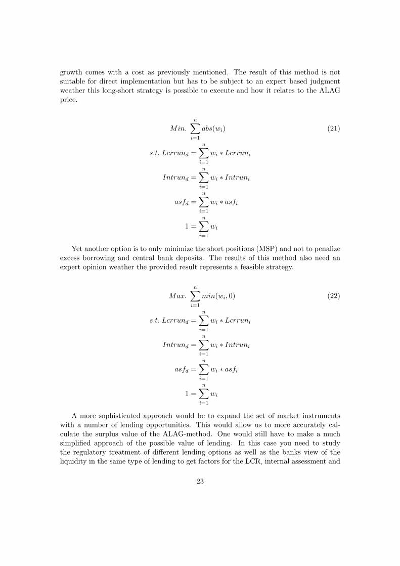
growth comes with a cost as previously mentioned. The result of this method is notsuitable for direct implementation but has to be subject to an expert based judgmentweather this long-short strategy is possible to execute and how it relates to the ALAGprice.

Min.n∑

i=1

abs(wi) (21)

s.t. Lcrrund =n∑

i=1

wi ∗ Lcrruni

Intrund =n∑

i=1

wi ∗ Intruni

asfd =

n∑i=1

wi ∗ asfi

1 =

n∑i=1

wi

Yet another option is to only minimize the short positions (MSP) and not to penalizeexcess borrowing and central bank deposits. The results of this method also need anexpert opinion weather the provided result represents a feasible strategy.

Max.

n∑i=1

min(wi, 0) (22)

s.t. Lcrrund =

n∑i=1

wi ∗ Lcrruni

Intrund =

n∑i=1

wi ∗ Intruni

asfd =

n∑i=1

wi ∗ asfi

1 =

n∑i=1

wi

A more sophisticated approach would be to expand the set of market instrumentswith a number of lending opportunities. This would allow us to more accurately cal-culate the surplus value of the ALAG-method. One would still have to make a muchsimplified approach of the possible value of lending. In this case you need to studythe regulatory treatment of different lending options as well as the banks view of theliquidity in the same type of lending to get factors for the LCR, internal assessment and

23

the NSFR. Instead of interest rate paid one needs to know what profit that could begenerated from each lending opportunity to then get the correct price of the deposit.This method demands many more parameters which might not be easily observable suchas the demand for loans preferably all over the curve but might be still be the fairestapproach for certain products that demands large short positions to be replicated in theMSP and MTA methods.

6 Discussion

The developed model offers some factors that can be used for predicting depositor be-havior but largely behavior is dependent on factors other than the ones that have beeninvestigated in this report. There seems to be some differences depending on indus-try belonging of depositors but the large impact of industry belonging when assessingdeposit value comes from regulatory constraints. Differentiating the current depositorbase only with regards to the banks own empirical experience does only motivate pricedifferences of a few basis points.

The other maybe more interesting result trying to put the price paid for depositsin the context of other funding sources where the deposit is described by parametersderived from the internal empirical experience as well as considering regulatory aspectof deposit usability shows that there is reason to differentiate prices with regards toseveral parameters (i.e. industry, average volume etc.).

The model gives prices related to costs of raising funding in the markets but it hasa weakness in not being sensitive to lending opportunities and hence an implementationwithout close monitoring of the effects might lead to paying more for the funding receivedthan received from lending creating an ”Ebberods Bank”. The obvious next step indeveloping this model should be to look at if an Ebberods-factor should be applied tocalculated deposit prices if balance sheet assets do not generate enough income to coverfor cost of liabilities.

24

7 Biography

Fred A. Poorman (2001), Using Physical Models to describe and Value Core Deposits,Winter 2001–2002. Bank Accounting and Fianance

Timothy H. Hannan and Robin A. Prager, Multimarket bank pricing: An empirical in-vestigation of deposit interst rates, Journal of Economics and Business 58 (2006) 256–272

Richard G. Sheehan (2004), Valuing Core Deposits, Springer

Basel Committee on Banking Supervision (2013), Basel III: International framework forliquidity risk measurement, standards and monitoring

Andreas Blochlinger and Marie Basile (2010) Optimal Deposit Pricing: There is no’One-Size-FitsAll’ Valuation Approach

Jean Dermine (2011), Fund Transfer Pricing for Deposits and Loans Foundation andAdvanced, Working Paper

25

TRITA-MAT-E 2013:20 ISRN-KTH/MAT/E—13/20-SE

www.kth.se