1

MODELING CREDIT RISK FOR SMES: EVIDENCE FROM THE US MARKET

Edward I. Altmana1 and Gabriele Sabatob2

a NYU Salomon Center, Leonard N. Stern School of Business, New York University, 44 West 4th Street, New York, NY 10012, USA

b Department of Banking, Faculty of Economics, University of Rome “La Sapienza”, via del Castro Laurenziano 9, 00161 Rome, Italy

Abstract

Considering the fundamental role played by small and medium sized

enterprises (SMEs) in the economy of many countries and the considerable attention placed on SMEs in the new Basel Capital Accord, we develop a distress prediction model specifically for the SME sector and to analyze its effectiveness compared to a generic corporate model. The behavior of financial measures for SMEs is analyzed and the most significant variables in predicting the entities’ credit worthiness are selected in order to construct a default prediction model. Using a logit regression technique on a panel of over 2,000 US firms (with sales less than $65 million) over the period 1994-2002, we develop a one-year default prediction model. This model has an out of sample prediction power which is almost 30% higher than a generic corporate model. An associated objective is to observe our model’s ability to lower bank capital requirements considering the new Basel Capital Accord’s rules for SMEs.

JEL classification: G21; G28 Key words: SME finance; Modeling credit risk; Basel II; Bank capital requirements

1 Corresponding author. E-mail address: ealtman@stern.nyu.edu Tel.: +1 212 998 0709. 2 Corresponding author. E-mail address: info@gabrielesabato.it Tel.: +31 6 51 39 99 07.

2

1. Introduction

Small and medium sized enterprises (SMEs) are reasonably considered the

backbone of the economy of many countries all over the world. For OECD

members, the percentage of SMEs out of the total number of firms is greater than

97%. In the US, SMEs provide approximately 75% of the net jobs added to the

economy and employ around 50% of the private workforce, representing 99.7% of

all employers1. Thanks to the simple structure of most SMEs, they can respond

quickly to changing economic conditions and meet local customers’ needs, growing

sometimes into large and powerful corporations or failing within a short time of the

firm’s inception. From a credit risk point of view, SMEs are different from large

corporates for many reasons. For example, Dietsch and Petey (2004) analyze a

panel of German and French SMEs and conclude that they are riskier but have a

lower asset correlation with each other than large businesses do. Indeed, we

hypothesize that applying a default prediction model developed on large corporate

data to SMEs will result in lower prediction power and likely a poorer performance

of the entire corporate portfolio than with separate models for SMEs and large

corporates.

The main goal of this paper is to analyze a rather complete set of financial

ratios linked to US SMEs and find out which are the most predictive ones of the

entities’ credit worthiness. One motivation of our study is to show the significant

importance for banks of modeling credit risk for SMEs separately from large

corporates. The only study that we are aware of that focused on modeling credit risk

specifically for SMEs is a fairly distant article by Edmister (1972). He analyzed 19

financial ratios and, using multivariate discriminant analysis, developed a model to

predict small business defaults. His study is carried on a sample of small and

medium sized enterprises over the period 1954-1969. We expand and improve his

1 Statistics provided by the United States Small Business Administration, www.sba.gov.

3

work using, for the first time, the definition of SME as contained in new Basel

Capital Accord (sales less than €50 million) and applying a logit regression analysis

to develop the model. We extensively analyze a large number of relevant financial

measures in order to select the most predictive ones. Then, we use these variables as

predictors of the default event. The final output is not only an extensive study of

SME financial characteristics, but also a model to predict their PD, specifically the

one year PD required under Basel II2. The performance of this model is also

compared with the performance of a well-known generic corporate model (known

as Z’’-Score3) in order to show the importance of modeling SME credit risk

separately from a generic corporate model. We acknowledge that our analysis could

still be improved using qualitative variables as predictors in the failure prediction

model to better discriminate between SMEs (as recent literature, e.g. Lehmann

(2003) and Grunet et al. (2004), demonstrate). The database that we use

(COMPUSTAT), however, does not contain qualitative variables. Nevertheless, the

performance accuracy of the model that we develop specifically to predict SME

default is significantly high both on an absolute and relative basis.

While there have been many successful models developed for corporate

distress prediction purposes, and at least two are commonly used by practitioners on

a regular basis4, none were developed specifically for SMEs. In addition, we feel

that the original Z-Score models (developed by one of the authors) can be improved

upon by transforming several of the variables to adjust for the changing values and

distributions of several of the key variables of that model. We feel that a

parsimonious selection of variables, some of which are transformed, can

2 Basel Committee on Banking Supervision, June 2004. 3 This is a model for manufacturing and non manufacturing firms, see Altman and Hotchkiss (2005). This model is of the form Z’’-Score= 6.56X1+3.26X2+6.72X3+1.05X4, where : X1= working capital/total assets; X2=retained earnings/total assets; X3=EBIT/total assets; X4=book value equity/total assets. 4 We refer to the KMV model, now owned and marketed by Moody’s/KMV, and the Altman Z-Score model (available from Bloomberg, S&P’s Compustat and several other vendors).

4

compensate for the fact that our model cannot make use of qualitative variables that

are available only from banks and other lending institutions files5.

The analysis is carried out on a sample of 2,010 US firms (with sales less than

$65 million)6 including 120 defaults, spanning the time period 1994 to 2002. In

Section 2, a survey of the most relevant literature about failure prediction

methodologies is provided. First, the choice of using a logistic regression to develop

a specific SME credit risk model is addressed and justified. Then, we give an

overview of the most recent studies about SMEs and we analyze their findings. In

Section 3, we develop a model to predict one-year SME default. We examine

different statistical alternatives to improve the performance of our model and

compare the results. Results using a logistical technique are contrasted with other

alternatives, principally discriminant analysis. In Section 4, the value of developing

a specific model in order to estimate SME one-year PDs is emphasized. In

particular, the benefits, in terms of lower capital requirements for banks of applying

a specific SME model are shown. We demonstrate that improving the prediction

accuracy of a credit risk model is likely to have beneficial effects on the Basel II

capital requirements for SMEs when the Advanced Internal Rating Based (A-IRB)

approach is used and, as such, could result in lower interest costs for SME

customers. In Section 5, we provide our conclusions.

5 We are aware that most large banks have recently been motivated to develop models specifically for SMEs since the new Basel Accord explicitly differentiates capital requirements between large corporates and SMEs. 6 This sales limit of $65 million (the equivalent of €50 million) comes from the new Basel Capital Accord’s definition of a SME (June 2004). Perhaps, $50 million in the US and A$50 million in Australia will be the definitions to be implemented in those countries. In our precedent work (Altman and Sabato, 2005), we have analyzed the different SME definitions for Europe, US and Australia and explored the expected capital requirements for SMEs under the Basel II Accord. We believe that banks now consider the Basel II definition as prominent.

5

2. Review of the relevant research literature

In this Section, we review some of the most important works about failure

prediction methodologies. First, we analyze the most popular alternative statistical

techniques that can be used to develop credit risk models and then we focus on the

works that have investigated the problem of modeling credit risk for small and

medium sized firms.

2.1 Default prediction studies

The literature about default prediction methodologies is huge. Many authors

during the last 40 years have examined several possible realistic alternatives to

predict customers’ default or business failure. The seminal works in this field were

Beaver (1967) and Altman (1968), who developed univariate and multivariate

models to predict business failures using a set of financial ratios. Beaver (1967) used

a dichotomous classification test to determine the error rates a potential creditor

would experience if he classified firms on the basis of individual financial ratios as

failed or non-failed. He used a matched sample consisting of 158 firms (79 failed

and 79 non-failed) and he analyzed 14 financial ratios. Altman (1968) used a

multiple discriminant analysis technique (MDA) to solve the inconsistency problem

linked to the Beaver’s univariate analysis and to assess a more complete financial

profile of firms. His analysis was on a matched sample containing 66 manufacturing

firms (33 failed and 33 non-failed) that filed a bankruptcy petition during the period

1946-1965. Altman examined 22 potentially helpful financial ratios and ended up

selecting five7 as doing the best overall job together in the prediction of corporate

bankruptcy. The variables were classified into five standard ratios categories,

including liquidity, profitability, leverage, solvency and activity ratios.

7 The original Z-score model (Altman, 1968) used five ratios: Working Capital/Total Assets, Retained Earnings/Total Assets, EBIT/Total Assets, Market Value Equity/BV of Total Debt and Sales/Total Assets.

6

For many years thereafter, MDA was the prevalent statistical technique

applied to the default prediction models and it was used by many authors (Deakin

(1972), Edmister (1972), Blum (1974), Eisenbeis (1977), Taffler and Tisshaw

(1977), Altman et al. (1977), Bilderbeek (1979), Micha (1984), Gombola et al.

(1987), Lussier (1995), Altman et al. (1995)). However, in most of these studies,

authors pointed out that two basic assumptions of MDA are often violated when

applied to the default prediction problems8. Moreover, in MDA models, the

standardized coefficients cannot be interpreted like the slopes of a regression

equation and hence do not indicate the relative importance of the different variables.

Considering these MDA’s problems, Ohlson (1980), for the first time, applied the

conditional logit model to the default prediction’s study9. The practical benefits of

the logit methodology are that it does not require the restrictive assumptions of

MDA and allows working with disproportional samples. Ohlson used a data set with

105 bankrupt firms and 2,058 non-bankrupt firms gathered from the COMPUSTAT

database over the period 1970-1976. He chose nine predictors (7 financial ratios and

2 binary variables) to carry on his analysis, mainly because they appeared to be the

ones most frequently mentioned in the literature. The performance of his models, in

terms of classification accuracy, was lower than the ones reported in the previous

studies based on MDA (Altman, 1968 and Altman et al., 1977), but he pointed out

some reasons to prefer the logistic analysis.

From a statistical point of view, logit regression seems to fit well the

characteristics of the default prediction problem, where the dependant variable is

binary (default/non-default) and with the groups being discrete, non-overlapping and

identifiable. The logit model yields a score between zero and one which

8 MDA is based on two restrictive assumptions: 1) the independent variables included in the model are multivariate normally distributed; 2) the group dispersion matrices (or variance-covariance matrices) are equal across the failing and the non-failing group. See Barnes (1982), Karels and Prakash (1987) and McLeay and Omar (2000) for further discussions about this topic. 9 Zmijewski (1984) was the pioneer in applying probit analysis to predict default, but, until now, logit analysis has given better results in this field.

7

conveniently gives the probability of default of the client10. Lastly, the estimated

coefficients can be interpreted separately as the importance or significance of each

of the independent variables in the explanation of the estimated PD. After the work

of Ohlson (1980), most of the academic literature (Zavgren (1983), Gentry et al.

(1985), Keasy and Watson (1987), Aziz et al. (1988), Platt and Platt (1990), Ooghe

et al. (1995), Mossman et al (1998), Charitou and Trigeorgis (2002), Lizal (2002),

Becchetti and Sierra (2002)) used logit models to predict default. Despite the

theoretic differences between MDA and logit analysis, studies show that empirical

results are quite similar in terms of classification accuracy. Indeed, after careful

consideration of the nature of the problems and of the purpose of this study, we have

decided to choose the logistic regression as an appropriate statistical technique. For

comparison purposes, however, we also analyze results using MDA.

2.2 SME studies

More recently, the new Basel Accord for bank capital adequacy (Basel II) has

driven the attention of many analysts to the SME segment (see for example

Schwaiger (2002), Saurina and Trucharte (2004), Udell (2004), Berger (2004),

Jacobson et al. (2004), and Altman and Sabato (2005)). Actually, many criticisms

have been raised by governments and SME associations that high capital charges for

SMEs could lead to credit rationing of small firms and, given the importance of

these firms in the economy, could reduce economic growth. The aforementioned

studies have dealt with the problem of the possible effects of Basel II on bank

capital requirements, but the problem of modeling credit risk specifically for SMEs

has not been addressed or only touched upon. Other authors have focused on the

difficulties and the potentials of small business lending, investigating the key drivers

of SME profitability and riskiness for US banks (Kolari and Shin (2004)) or the

10 Critics of the logit technique, including one of the authors of this paper, have pointed out the specific functional form of a logit regression can lead to bimodal (very low or very high) classification and probabilities of default.

8

lending structures and strategies (Berger and Udell (2004)). Recently, Berger and

Frame (2005) have analyzed the potential effects of the small business credit scoring

on credit availability. They find that banking organizations that implement

automated decision systems (such as scoring systems) increase small business credit

availability. They focus on micro business credits (up to $250.000) that were

managed with credit scoring from the latter half of 1990s in the US using personal

credit history of the principal owner provided by one or more of the consumer credit

bureaus (e.g. Equifax, Experian, FICO). However, today banks need to manage as

retail clients exposures toward SMEs up to at least €1 million (if they want to

consider the Basel II definition11) to be competitive in the credit business. We think

that the complexity of these bigger companies cannot be managed only with bureau

information, but a financial analysis is needed.

Following the large literature, we conclude that small business lending has a

strong positive effect on bank profitability (as Kolari and Shin (2004) and Berger

(2004) demonstrate), but we find, in contrast with Kolari and Shin (2004), that SME

business is riskier than large corporate lending (see also Saurina and Trucharte

(2004), Dietsch and Petey (2004)). As a consequence, we demonstrate that banks

should develop credit risk models specifically addressed to SMEs in order to

minimize their expected and unexpected losses. Many banks and consulting

companies already follow this practice of separating large corporates from small and

medium sized companies when modeling credit risk. But, in the academic literature,

a study that demonstrates the significant benefits of such a choice is lacking.

Actually, the study by Edmister (1972), focused only on the selection of the

financial ratios that can be useful in predicting SME failure, but did not explain why

small firms should be separated from large companies. The emphasis on SME

credits in today’s environment is far more prominent and we show that modeling

specific SME credit risk systems is likely, under certain sceneries, to lead to lower

11 We are aware of some large, international bank (such as Barclay) that is managing SMEs as retail clients using automated scoring systems for credits up to €3 million.

9

capital requirements when the new Basel Capital Accord will be implemented in

200812.

3. SME model development

In this Section, we develop a specific model to estimate one-year SME

probability of default. We illustrate the steps of our analysis and compare the results

obtained using different statistical instruments (such as log transformations of the

variables). Statistical details about the developed models can be found in the

Appendixes.

3.1 The data set

The statistical analysis utilized a sample containing financial data of 2,010

US SMEs with sales less than $65 million (approximately €50 million), gathered

from WRDS COMPUSTAT database over the period 1994-200213. To create this

sample, we first assessed the number of defaulted firms contained in the

COMPUSTAT database during the selected period and we find 120 defaulted SMEs

(with non-missing data) 14. Then, we randomly select non-defaulted firms over the

same period in order to obtain an average default rate in our sample as close as

possible to the expected average default rate for US SMEs (6%)15. We use this

expected average default rate as a prior probability input in our retrospective

analysis16. For each selected year, the number of non-defaulted SMEs has been

12 A recent directive extended the introduction in the US one year beyond 2007; 2007 is still the expected implementation date in Europe. 13 COMPUSTAT North America (Standard & Poor’s Corp., a division of Mc Graw-Hill Corp.) is a database of US and Canadian financial and market information on more than 24,000 active and inactive publicly held companies. 14 “TL” footnote is used to indicate firms in bankruptcy, while “AG” means that the firm is in reorganization. 15 This expected average default rate for US SMEs has been suggested to us from a Moody’s study about small and medium sized firms in the US, “Moody’s KMV Riskcalc v3.1 Model”, April 2004. 16 See McFadden (1973) and King and Zeng (2001) for a comprehensive analysis of the use of the prior probability in the logit model.

10

calculated in order to maintain the overall average expected default rate.

Subsequently, we have randomly selected, for each year, the number of non-

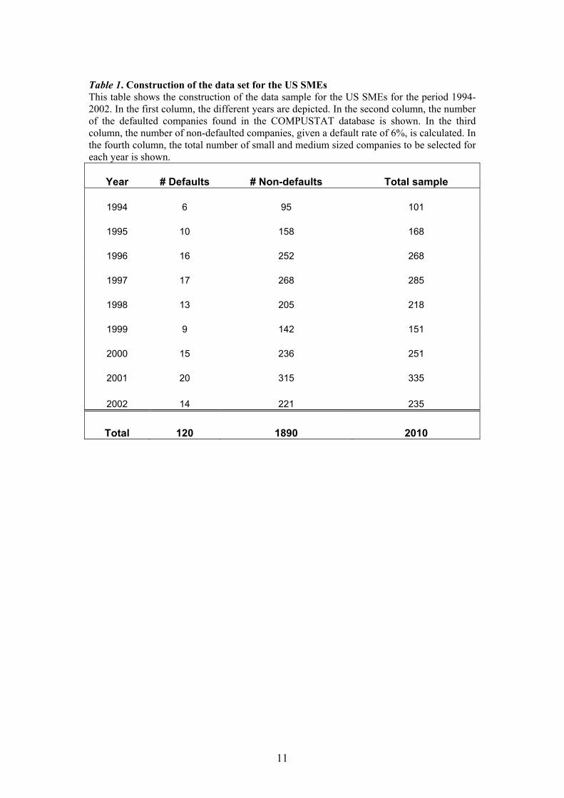
defaulted firms shown in the third column of Table 1. The total of 120 defaults and

1,890 non-defaults are shown at the bottom of that table. In order to provide a

picture of small and medium sized enterprises contained in our sample, in the

Figures 1 and 2 we show the distribution of their sales and total assets. Note that

SMEs might be somewhat arbitrarily classified as either small or medium sized

firms using either sales or assets as the size criteria.

11

Table 1. Construction of the data set for the US SMEs This table shows the construction of the data sample for the US SMEs for the period 1994-2002. In the first column, the different years are depicted. In the second column, the number of the defaulted companies found in the COMPUSTAT database is shown. In the third column, the number of non-defaulted companies, given a default rate of 6%, is calculated. In the fourth column, the total number of small and medium sized companies to be selected for each year is shown.

Year # Defaults # Non-defaults Total sample

1994 6 95 101

1995 10 158 168

1996 16 252 268

1997 17 268 285

1998 13 205 218

1999 9 142 151

2000 15 236 251

2001 20 315 335

2002 14 221 235

Total 120 1890 2010

12

Figure 1. Distribution of sales in the US SME sample This figure shows the percentage of US SMEs contained in each of four sales classes in our sample. The four size classes could be divided into two groups: ones with sales less than $25 million (small firms) (68.4%) and the ones with sales between $26 and $65 million (medium firms) (31.6%).

12.2%51-65

19.4%26-50

22.2%16-25

46.2%<15

Category<1516-2526-5051-65

Sales Class (MM$)

Figure 2. Distribution of assets in the US SME sample This figure shows the percentage of US SMEs contained in each of five asset classes in our sample. The five asset classes could be divided into two groups: ones with assets less than $25 million (small firms) (56.2%) and the ones with assets more than $25 million (medium firms) (43.8%).

11.6%> 100

16.1%51-100

16.0%26-50

20.2%16-25

36.0%<15

Category

> 100

<1516-2526-5051-100

Assets Class (MM$)

13

3.2 Selection of the variables

There is a large number of possible candidate ratios that in the literature have

been found useful to predict firms’ default17. Furthermore, recent literature (e.g.

Lehmann (2003) and Grunet et al. (2004)) concludes that quantitative variables are

not sufficient to predict SME default and that qualitative variables (such as the

number of employees, the legal form of the business, the region where the main

business is carried out, the industry type, etc.) are useful in improving the models’

prediction power. In this study, we are obliged to use only firms’ financial statement

data since the COMPUSTAT database does not contain qualitative variables18.

Consistent with the large number of studies discussed in Section 2, we

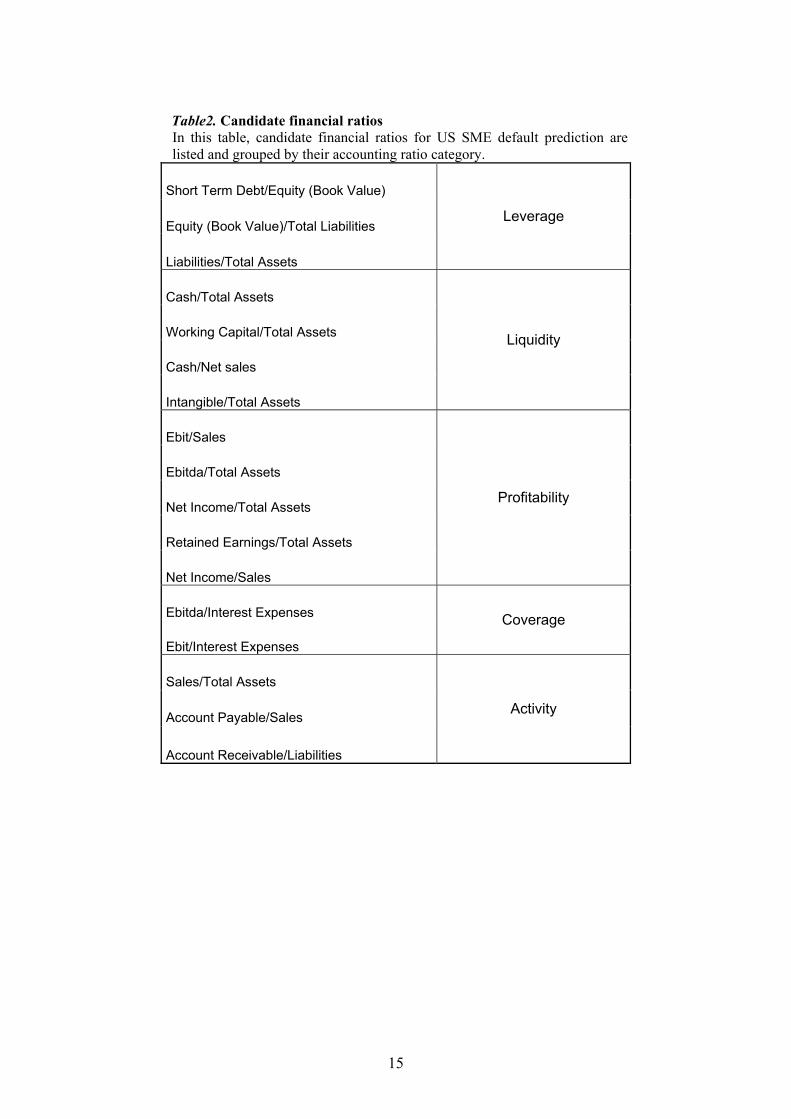
choose five accounting ratio categories describing the main aspects of a company’s

financial profile: liquidity, profitability, leverage, coverage and activity. For each

one of these categories, we create a number of financial ratios that were most

successful in predicting firms’ bankruptcy in the existing studies (see Table 2). We

also graphically analyzed the relationship between the 17 financial ratios selected

and the default event to check if their behavior follows our expectations (see

Appendix A for a detailed discussion).

After the potential candidate predictors have been defined and calculated, we

observe the accuracy ratio (as defined by Keenan and Sobehart (1999)) for each and

arbitrarily select two variables from each group with the highest accuracy. Since this

analysis does not take into account the possible correlations between the variables in

each group, we decided to select two variables from each ratio category rather than

one. Next, we apply a statistical forward stepwise selection procedure of the selected

ten variables19. We then estimate the full model eliminating the least helpful 17 Chen and Shimerda (1981) show that out of more than 100 financial ratios, almost 50% were found useful in at least one empirical study. 18 In a recent work, Zhou et al. (2005) develop a model for North American privately held firms (not only SMEs) using a maximum expected utility (MEU) model. They gather data from S&P’s Credit Risk Tracker database, selecting 20 explanatory variables and separating their sample into four relevant groups of industries. The performance of their model is very promising and slightly higher than a model developed using the same variables and a logistic technique. However, we believe that separating the industry groups played an important role in improving the performance of their model. 19 In some statistical studies, criticism of the forward stepwise selection procedure has been raised as it can yield theoretically implausible models and select irrelevant variables. For this reason, we use a

14

covariates, one by one, until all the remaining input variables are efficient, i.e. their

significance level is below the chosen critical level. For this study, the significance

level is set at 20%. Of the ten chosen variables (see Table 3), five variables are

selected as doing the best overall job together in the prediction of the SME default

(see Table 4). Lastly, observing the default event, we construct the dependent

variable, Known Probability of Being Good (KPG), as binary (0=defaulted/1=non-

defaulted)20. Actually, we note that the firms considered as defaulted in this study

are the ones that went bankrupt under Chapter 11 of the US bankruptcy Code.

Observing the distributions of each of the selected variables for the two

dependent variable groups, a large range of values is clearly visible. This high

variability of the financial ratios for SMEs can be due either to the different sectors

in which these companies operate (real estate firms have financial data completely

different from agricultural companies), or to the different ages of the firms in the

sample as well as their different level of financial health. We therefore use

logarithmic transformations for all of the five selected variables in order to reduce

the range of possible values and possibly increase the importance of the information

given by each one of them. To prove the effectiveness of this choice, we provide and

compare the analyses and the results obtained utilizing the logged and unlogged

predictors. We also expect that the higher accuracy level of the logged variable

structure will compensate somewhat for the lack of availability of qualitative data.

two-step analysis, first choosing the most relevant variables for our study and then applying the stepwise selection procedure. See also Hendry and Doornik (1994). 20 We use as dependent variable KPG in order to have positive slopes and intercept since the higher the final logit score, the higher the probability than the firm will not fail.

15

Table2. Candidate financial ratios In this table, candidate financial ratios for US SME default prediction are listed and grouped by their accounting ratio category.

Short Term Debt/Equity (Book Value)

Equity (Book Value)/Total Liabilities

Liabilities/Total Assets

Leverage

Cash/Total Assets

Working Capital/Total Assets

Cash/Net sales

Intangible/Total Assets

Liquidity

Ebit/Sales

Ebitda/Total Assets

Net Income/Total Assets

Retained Earnings/Total Assets

Net Income/Sales

Profitability

Ebitda/Interest Expenses

Ebit/Interest Expenses

Coverage

Sales/Total Assets

Account Payable/Sales

Account Receivable/Liabilities

Activity

16

Table3. First step of the variable selection process This table shows the ten financial ratios (two for each accounting ratio category) that presented the highest accuracy between all of the candidate financial ratios.

Short Term Debt/Equity (Book Value)

Liabilities/Total Assets

Leverage

Cash/Total Assets

Working Capital/Total Assets

Liquidity

Ebitda/Total Assets

Retained Earnings/Total Assets

Profitability

Ebitda/Interest Expenses

Ebit/Interest Expenses

Coverage

Sales/Total Assets

Account Receivable/Liabilities

Activity

17

Table4. Selected financial ratios for US SMEs In this table, the selected financial ratios, after a two step selection process, for the US SME model are listed and grouped by their accounting ratio category. In the last column, the univariate explanatory power statistic (Gini index) of each ratio is shown. The Gini index measures the ability of a variable (or a scorecard) to concentrate defaulted customers on lower scores compared to the percentage of non-defaulted clients concentrated on higher scores. The level of this concentration is measured by the GINI coefficient. The minimum value is 0, while the (theoretical) maximum value is 1.

G3 Short Term Debt/Equity Book Value Leverage 14.57%

G9 Cash/Total Assets Liquidity 18.73%

G2 Ebitda/Total Assets 20.58%

G5 Retained Earnings/Total Assets

Profitability

22.62%

G10 Ebitda/Interest Expenses Coverage 21.10%

18

3.3 Logistic regression

First, we run the logistic regression using the unlogged variables (a detailed

discussion of this model is provided in Appendix B). All of the slopes (signs) follow

our expectations (i.e. we expect a positive relationship between the KPG and all the

predictors except Short term debt/BV of Equity, as discussed in Appendix A) and

the Wald test for each of the predictors is statistically significant21. Also the Log-

likelihood test is statistically significant, i.e. we can argue that there is a significantly

strong relationship between the selected predictors and the default event22. The

Hosmer-Lemeshow test (Hosmer and Lemeshow, 1989), which is used to

understand whether using an appropriate statistical technique (in this case the

logistic regression), is statistically significant (P value equal to 0.421) as we were

not making an appropriate choice using the logistic regression. However, the result

of the Hosmer-Lemeshow test can be misleading since it can be due only to the wide

range of values of the original predictors. Lastly, we observe the measures of

association (Somers’ “D”, Goodman and Kruskal’s “Gamma” and Kendall’s “Tau-

b”) to compare this model with the one developed utilizing the logarithmic values of

the predictors. We depict our first model in Table 5, where the final score (that can

be approximated with the probability that a firm does not default) is given by the

sum of the constant (4.28) and the product between the slopes and the value of each

of the predictors.

As we will demonstrate, the results are fairly accurate, but the accuracy ratio

(75%) certainly could be improved to give us more confidence in the reliability of

the model.

21 The Wald test, described by Polit (1996) and Agresti (1990), is a way to test whether the parameters associated with a group of explanatory variables are zero, or not. 22 The Log-likelihood test is used to understand if all the parameters together are useful to estimate the dependent variable. It is comparable to the multivariate F-Test in the linear regressions (or MDA) and it is also often used to compare the fit of different models (see Dunning 1993).

19

Table5. Model developed with unlogged predictors

This table shows the model developed using the unlogged values of the variables to predict the probability of non-defaulting (KPG).

KPG = + 4.28

+ 0.18 Ebitda/Total Assets

- 0.01 Short Term Debt/Equity Book Value

+ 0.08 Retained Earnings/Total Assets

+ 0.02 Cash/Total Assets

+ 0.19 Ebitda/Interest Expenses

20

We then utilize the logarithmic transformed predictors in an attempt to

increase the accuracy of the model. The EBITDA/total assets (EBITDA/TA) and the

retained earnings/total assets (RE/TA) variables, following Altman and Rijken

(2004), are transformed as follows: EBITDA/TA → -ln(1-EBITDA/TA), RE/TA →

-ln(1-RE/TA). Actually, the distributions of these two variables are negatively

skewed and the information content in the fat tails of the distribution is relatively

low. So, with this transformation we can give more power to the values that are

more significant for the regression. Moreover, in this way we are somewhat able to

correct for the trend of the unlogged variables which were continuously drifting

down over the years. For example, the RE/TA variable had a mean absolute value in

1980 of almost 20 percentage points higher than the average value for US

companies in 2004. The other three variables have the standard log transformation.

After these transformations, the regression results look much more promising (see

Appendix C for a detailed discussion of this model’s development). Wald and Log-

likelihood tests are statistically significant as before and the slopes are all reasonable

(see Table 6). This time, the Hosmer-Lemeshow test is not statistically significant (P

value equal to 0.978). The measures of associations show higher values than before,

suggesting that the revised model should have higher prediction accuracy. The

accuracy ratio jumped from 75% to 87% when we transformed each of the original

firm variables by using their logarithms. However, to decide if the revised model is

really better than the one built with the original predictors, we test and compare their

prediction accuracy on a hold-out sample.

21

Table6. Model developed with logged predictors

This table shows the model developed using the logged values of the variables to predict the probability of non-defaulting (KPG).

KPG = + 53.48

+ 4.09 -LN(1-Ebitda/Total Assets)

- 1.13 LN(Short Term Debt/Equity Book Value)

+ 4.32 -LN(1-Retained Earnings/Total Assets)

+ 1.84 LN(Cash/Total Assets)

+ 1.97 LN(Ebitda/Interest Expenses)

22

3.4 Validation results

In order to test the validation performance of our models, we assemble a

holdout sample of 26 bankrupt SMEs for the two-year period 2003-200423. Then, we

randomly select non-bankrupt companies over the same recent two-year period

using the methodology explained before. The test sample contains a total of 432

firms (bankrupt and non-bankrupt) with sales less than $65 million (see Table 7).

In Table 8, we summarize the results, in terms of predictive accuracy of the

three different models (the two logistic models developed with logged and unlogged

predictors and a generic corporate model) tested on the hold-out sample. As generic

corporate model, we use the Z’’-Score model developed by Altman in 1993 (see

footnote number 3 for details). The error rates shown in Table 8 are calculated fixing

an arbitrary cut-off rate of 30% of the population24 and are quite close to the error

rates obtained from the development sample (in the same Table 8, but in brackets).

Hence, we can argue that the models are statistically robust and valid. We

acknowledge that the chosen cut-off rate is possibly not the optimal one since the

different misclassification costs for the type I and type II error rates are not taken

into account (see Altman et al. (1977) and Taffler (1982)). However, we point out

that the purpose of this work is to use a common, arbitrary, fixed cut-off rate only to

compare the prediction accuracy of the different models and not to find the best cut-

off strategy. Moreover, we believe that the optimum cut-off value cannot be found

without a careful consideration of each particular bank peculiarities (e.g. tolerance

for risk, profit-loss objectives, recovery process costs and efficiency, possible

marketing strategies).

23 Again, we use the WRDS COMPUSTAT tapes. 24 Applying the developed model to all the companies contained in the test sample, a score is calculated for each firm. Then, the 30% of the sample with the lowest scores is considered rejected in order to check the accuracy of the model to correctly and incorrectly classify the firms (as defaulted and non-defaulted) between accepted and rejected clients.

23

Table 7. Hold-out sample for SMEs

This table shows the structure of the US SME hold-out test sample. In the first and second row, the number and the percentage of non-defaulted and defaulted firms are shown.

Number Percentage

Non-defaulted firms 406 94.0%

Defaulted firms 26 6.0%

Total 432 100%

24

3.5 Comparison of results

In order to compare our results we provide two indexes (columns 4 and 5 in

Table 8). The first one measures the accuracy of each model in correctly classifying

defaulted and non-defaulted firms, as the complement of the weighted average of the

type I and type II error rates. The second index is called the accuracy ratio (AR) and

is defined as the ratio of the area between the cumulative accuracy profile (CAP) of

the rating model being validated and the CAP of the random model, and the area

between the CAP of the perfect rating model and the CAP of the random model (see

Engelman et al. (2003) for further details). Indeed, it measures the ability of the

model to maximize the distance between the defaulted and non-defaulted clients.

The overall accuracy level (AR) of our two new logistic models is 75%,

based on the unlogged variables, and 87% based on the logged variables. Most

importantly, the type I error is reduced dramatically when we use the logged

variables model from over 21% to 11.76%. Also in Table 8, we compare the holdout

results with the popular Z’’-Score results built by Altman (1993) to include all

industrial firms25. Applying the four variable Z’’-Score model to the same holdout

sample, we observe an overall accuracy (AR) of 68%, compared to the 75% for the

unlogged new variable model and the 87% for the logged structural approach.

Again, the biggest improvement between the new model and the generic Z’’-Score

approach was in the type I accuracy.

25 See footnote number 3 for details about the Z’’-Score model.

25

Table 8. Misclassification rates and accuracy ratios of the different models This table shows the misclassification rates and the accuracy ratios of the three different models applied to the test sample fixing an arbitrary cut-off rate of 30%. The first column shows the type I error rate, i.e. the percentage of defaulted firms classified as non-defaulted. In the second column, the type II error rate is illustrated. This rate represents the percentage of non-defaulted firms classified as defaulted. The third column shows the average accuracy of the model, calculated as 1 minus the average of the two error rates. In the last column, the accuracy ratio, defined as the ratio of the area between the cumulative accuracy profile (CAP) of the rating model being validated and the CAP of the random model, and the area between the CAP of the perfect rating model and the CAP of the random model, is shown. The values in the brackets result from the application of the different models on the development sample.

Type I error

rate Type II error

rate 1- Average Error Rate

Accuracy ratio

Logistic model developed with logarithm transformed predictors

11.76% (9.23%)

27.92% (24.64%)

80.16% (83.07%)

87.22% (89.81%)

Logistic model developed with original predictors

21.63% (20.11%)

29.56% (27.86%)

74.41% (76.02%)

75.43% (77.68%)

Z’’-Score Model 25.81% (26.12%)

29.77% (29.52%)

72.21% (72.18%)

68.79% (68.57%)

26

3.6 Multivariate Discriminant Analysis (MDA)

For comparison purposes, we also run a multivariate discriminant analysis

(MDA) model using the same development sample as we used for the logistic

analysis. In this case, we define two groups maintaining the original number of firms

in our sample (1890 non-defaulted firms and 120 defaulted firms). The same five,

log transformed financial measures, as the ones selected for the logistic analysis, are

utilized as predictors also for MDA. In Table 9, we show the model developed with

the MDA.

We observe that the ability of this model to separate the two groups is

notably lower (see Table 10) than the one developed with the logistic regression

(62% accuracy ratio versus almost 78% and 89% measured on the development

sample). Moreover, we find that the performance of the MDA model, in terms of

maximizing the distance between the two groups (defaulted and non-defaulted

firms), is even lover than the performance of the Z’’-Score model, developed using

MDA, but on data from large corporate firms.

We find that the power of the different financial measures that can be used to

predict firms’ financial distress is strictly linked to the statistical technique used to

develop the prediction model. In this case, the five financial ratios selected for the

logistic analysis do a less accurate overall job together than the five ratios selected

by Altman (1993) in his Z’’-Score model when MDA is chosen as appropriate

statistical technique. Also, in all cases, the ability of MDA models to discriminate

between defaulted and non-defaulted firms is lower than logistic models, at least

using the same predictors.

27

Table9. MDA model developed with logged predictors

This table shows the model developed using multivariate discriminant analysis to predict the probability of non-defaulting.

KPG = + 15.06

+ 2.44 -LN(1-Ebitda/Total Assets)

+ 0.91 LN(Short Term Debt/Equity Book Value)

+ 3.90 -LN(1-Retained Earnings/Total Assets)

+ 4.15 LN(Cash/Total Assets)

+ 3.49 LN(Ebitda/Interest Expenses)

28

Table 10. Misclassification rates and accuracy ratios for MDA methodology This table shows the misclassification rates and the accuracy ratios of the model developed using MDA methodology applied to the test sample fixing an arbitrary cut-off rate of 30%. The first column shows the type I error rate, i.e. the percentage of defaulted firms classified as non-defaulted. In the second column, the type II error rate is illustrated. This rate represents the percentage of non-defaulted firms classified as defaulted. The third column shows the average accuracy of the model, calculated as 1 minus the average of the two error rates. In the last column, the accuracy ratio, defined as the ratio of the area between the cumulative accuracy profile (CAP) of the rating model being validated and the CAP of the random model, and the area between the CAP of the perfect rating model and the CAP of the random model, is shown. The values in the brackets result from the application of the MDA model on the development sample.

Type I error rate

Type II error rate

1- Average Error Rate

Accuracy ratio

MDA model developed with logarithm transformed predictors

30.12% (29.63%)

29.84% (28.74%)

71.52% (73.32%)

59.87% (62.44%)

29

4. Basel II capital requirements for SMEs

In this Section, we show that improving the prediction accuracy of a credit risk

model is likely to have beneficial effects on the Basel II capital requirements for

SMEs when the Advanced Internal Rating Based (A-IRB) approach is used. Indeed,

applying a model with a higher accuracy discrimination power will result in lower

capital requirements regardless if the SMEs are all classified as retail customers or

as corporates. The new Basel Capital Accord permits banks the possibility to choose

whether to classify firms (with sales less than €50 million and exposure less than €1

million) as corporate or as retail. But, the Accord also requires that banks manage

SMEs on a pooled basis in order to be allowed to consider them as retail customers

and to apply the retail formula to calculate their capital requirement26.

The concept of “pool-management” for SMEs is not clearly explained by the

Accord and has been the source of some concern for banks. However, we believe

that the main motivation for the Basel Committee is that many banks, following this

requirement, will abandon old forms of relationship management used with SMEs

and go towards the use of more efficient automated decision systems (such as

scoring and rating systems). In our previous work (Altman and Sabato (2005)), we

examine the potential issues that banks can face when setting their internal systems

and procedures to manage SMEs on a pooled basis and we calculate the potential

capital requirements dependent on what proportion of the bank’s SME portfolio is

considered as retail or corporate. We conclude that most banks will use a blended

approach, classifying a part of the SME portfolio as retail and a part as corporate. As

such, we calculate the likely breakeven ratio of retail versus corporate for SME

customers.

26 In the US, only large, internationally active banks (core banks) will be required to adopt the A-IRB approach on a mandatory basis, while the other organizations will more than likely remain Basel I banks. This process can create competitive advantages for the biggest banking organizations (see Berger 2004). As such, US regulators are now considering a new type of regulatory capital known as Basel IA, for those banks choosing to not utilize the advanced IRB approach (see Board of Governors of the Federal Reserve, September 30, 2005).

30

In this study, we demonstrate the greater ability of a specific SME credit risk

model to separate non-failed from failed firms compared to a generic corporate

model (see Tables 11 to 14). We analyze the impact on capital requirements if the

entire SME portfolio was considered as retail or as corporate, respectively. We

apply two models (Z’’-Score and the newly developed, logistic model specific for

SMEs) to our sample to compare results. We are able to create seven rating classes

with both models. For each rating class, the probability of default (PD) is calculated

by dividing the number of defaults by the total number of enterprises in each class.

Rating classes have been created in order to obtain the value of PD closest to the one

showed by bond equivalent PD distributions. A fixed loss given default (LGD) of

45% is assumed, using the one suggested in the Foundation IRB approach (F-IRB)

for senior, unsecured loan exposures27, and the percentage of firms in each rating

class is used as the weight for the capital requirement (instead of the dollar amount

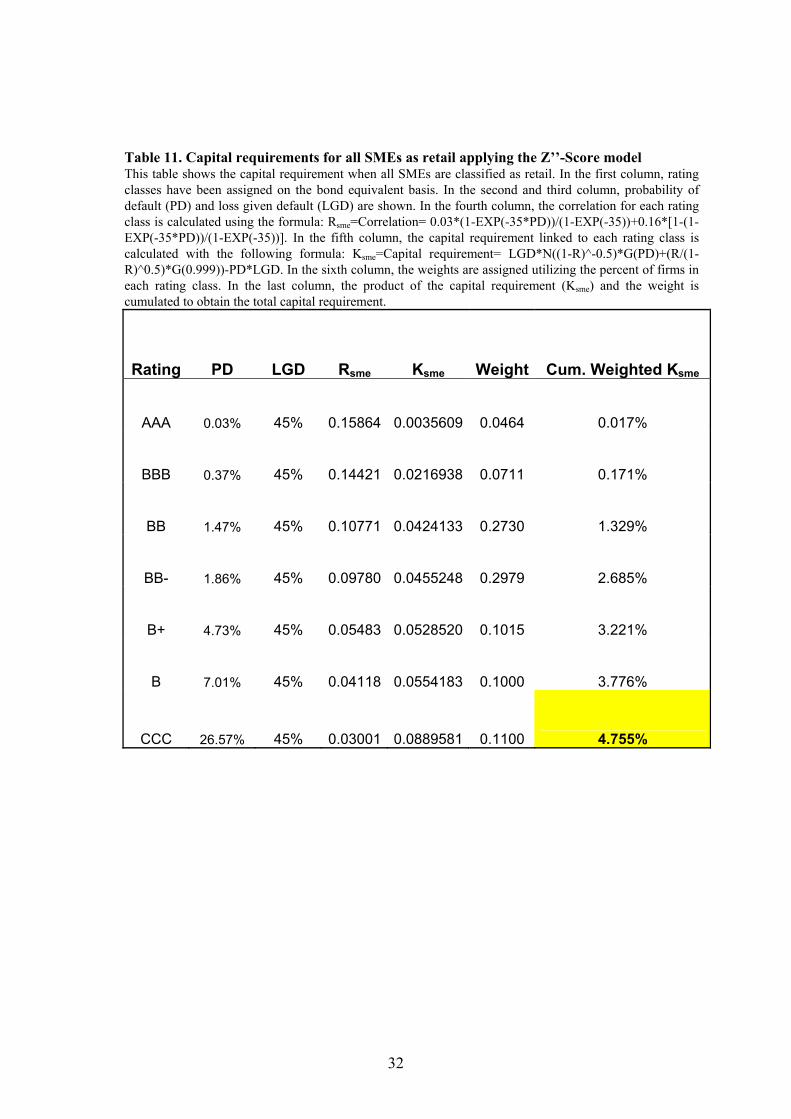
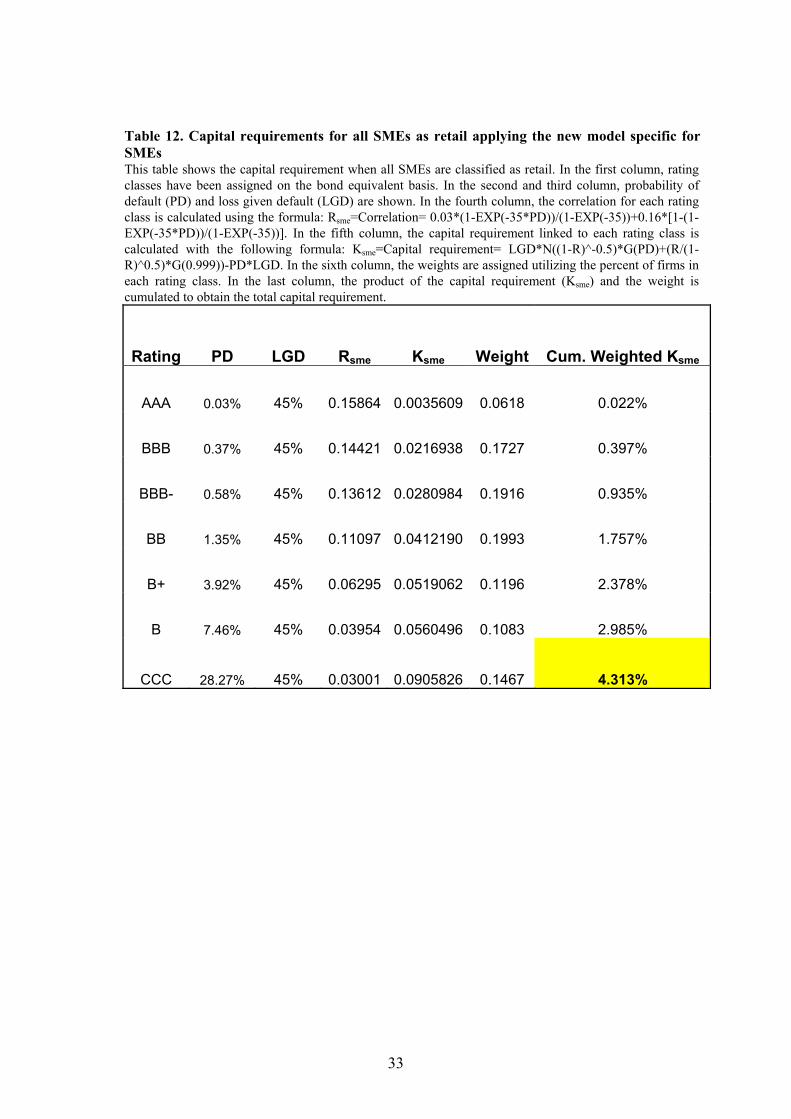
of the loan exposures). Classifying all SMEs as retail, we obtain a capital

requirement of 4.76%, using the Z’’-Score model, and of 4.31%, using the specific

model for SMEs (Tables 11 and 12). Both models results in capital requirements

considerably below the current 8% level, under Basel I.

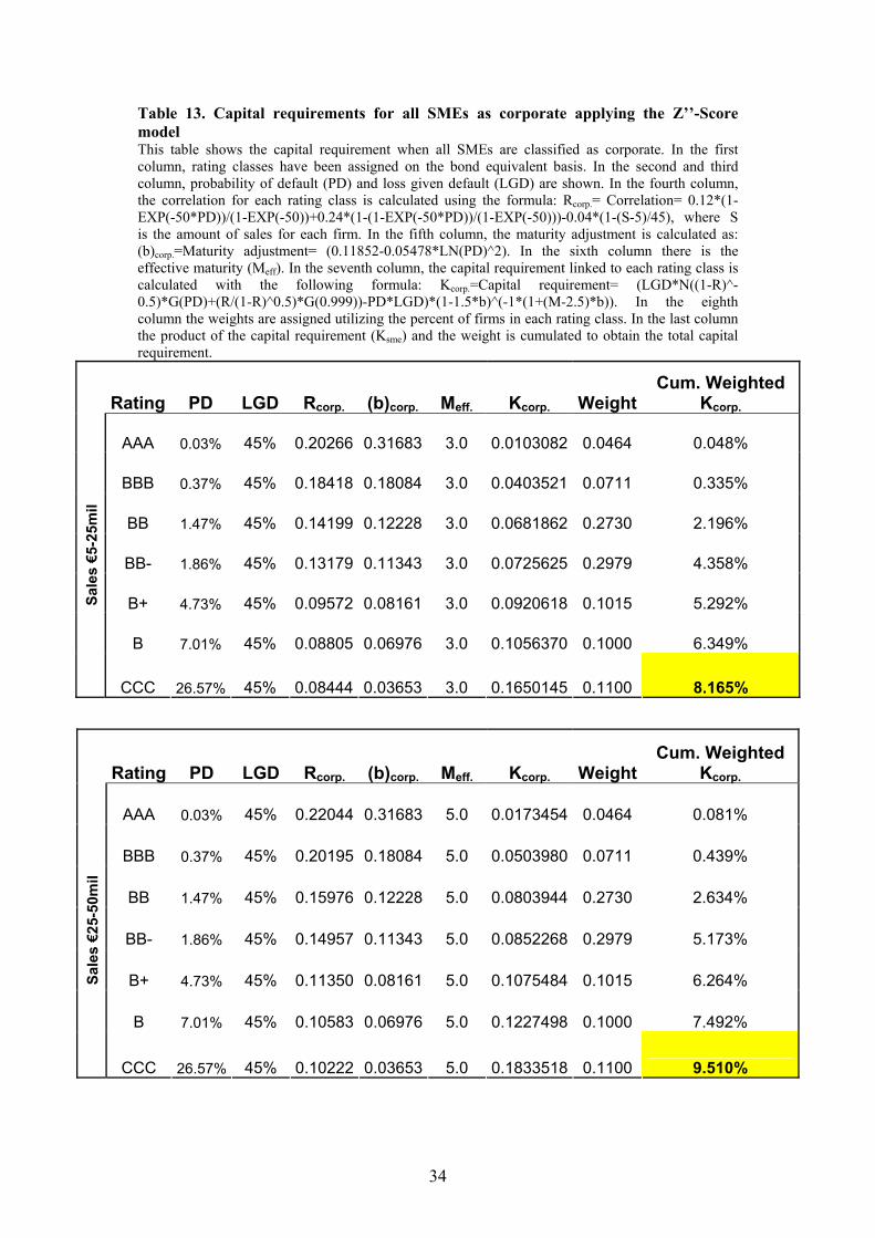
To consider SMEs as corporate (Tables 13 and 14), we have to make two

additional assumptions. The first is the effective maturity (Meff.). We select possible

maturities of three years for smaller firms and five years for medium sized firms.

The maturity adjustment ((b)corp.) is a function only of PD. The second assumption is

about the amount of sales to use for the size adjustment. We split the SME

population into two groups: one with sales between €5 and €25 million (small) and

the other with sales between €26 and €50 million (medium). In this way we use an

average amount of sales of €10 and €30 million in each size group, respectively28.

The two groups’ percentages of capital requirements are aggregated, considering

27 Basel Committee on Banking Supervision, June 2004, par. 287. 28 These average amounts are based on the realistic assumption that each sales distribution is skewed with more relatively small borrowers than relatively large borrowers (see also Altman and Sabato, 2005).

31

their distribution of sales for the two classes (68% for small and 32% for medium

sized firms). The resulting weighted capital requirements of the two size

components of SMEs, calculated in Tables 12 and 13, are 8.60%

(0.68*8.17+0.32*9.51), applying the Z’’-Score model, and 8.10%

(0.68*7.69+0.32*8.98), applying the new specific model for the SMEs.

The results of this study show that if banks classify their entire SME portfolio

as corporate using the A-IRB approach, they will likely face higher capital

requirements than under the current Basel I. And, we want to emphasize that this

result is even more representative if banks do what we propose, i.e. apply a specific

SME credit risk model with a very high prediction accuracy (87% in this case). The

capital requirement will still show a value (8.10%), slightly higher than the current

8%. Of course, it is possible that an even more accurate SME model could be

developed resulting in a capital requirement slightly lower than the current 8%. In

any case, capital requirements are considerably lower the greater the percentage of a

bank’s SME portfolio that can be classified as retail customers, but it may not be

possible for some banks to classify a large proportion as retail. Also, in all cases, the

better the credit scoring model, the lower the capital requirements.

32

Table 11. Capital requirements for all SMEs as retail applying the Z’’-Score model This table shows the capital requirement when all SMEs are classified as retail. In the first column, rating classes have been assigned on the bond equivalent basis. In the second and third column, probability of default (PD) and loss given default (LGD) are shown. In the fourth column, the correlation for each rating class is calculated using the formula: Rsme=Correlation= 0.03*(1-EXP(-35*PD))/(1-EXP(-35))+0.16*[1-(1-EXP(-35*PD))/(1-EXP(-35))]. In the fifth column, the capital requirement linked to each rating class is calculated with the following formula: Ksme=Capital requirement= LGD*N((1-R)^-0.5)*G(PD)+(R/(1-R)^0.5)*G(0.999))-PD*LGD. In the sixth column, the weights are assigned utilizing the percent of firms in each rating class. In the last column, the product of the capital requirement (Ksme) and the weight is cumulated to obtain the total capital requirement.

Rating PD LGD Rsme Ksme Weight Cum. Weighted Ksme

AAA 0.03% 45% 0.15864 0.0035609 0.0464 0.017%

BBB 0.37% 45% 0.14421 0.0216938 0.0711 0.171%

BB 1.47% 45% 0.10771 0.0424133 0.2730 1.329%

BB- 1.86% 45% 0.09780 0.0455248 0.2979 2.685%

B+ 4.73% 45% 0.05483 0.0528520 0.1015 3.221%

B 7.01% 45% 0.04118 0.0554183 0.1000 3.776%

CCC 26.57% 45% 0.03001 0.0889581 0.1100 4.755%

33

Table 12. Capital requirements for all SMEs as retail applying the new model specific for SMEs This table shows the capital requirement when all SMEs are classified as retail. In the first column, rating classes have been assigned on the bond equivalent basis. In the second and third column, probability of default (PD) and loss given default (LGD) are shown. In the fourth column, the correlation for each rating class is calculated using the formula: Rsme=Correlation= 0.03*(1-EXP(-35*PD))/(1-EXP(-35))+0.16*[1-(1-EXP(-35*PD))/(1-EXP(-35))]. In the fifth column, the capital requirement linked to each rating class is calculated with the following formula: Ksme=Capital requirement= LGD*N((1-R)^-0.5)*G(PD)+(R/(1-R)^0.5)*G(0.999))-PD*LGD. In the sixth column, the weights are assigned utilizing the percent of firms in each rating class. In the last column, the product of the capital requirement (Ksme) and the weight is cumulated to obtain the total capital requirement.

Rating PD LGD Rsme Ksme Weight Cum. Weighted Ksme

AAA 0.03% 45% 0.15864 0.0035609 0.0618 0.022%

BBB 0.37% 45% 0.14421 0.0216938 0.1727 0.397%

BBB- 0.58% 45% 0.13612 0.0280984 0.1916 0.935%

BB 1.35% 45% 0.11097 0.0412190 0.1993 1.757%

B+ 3.92% 45% 0.06295 0.0519062 0.1196 2.378%

B 7.46% 45% 0.03954 0.0560496 0.1083 2.985%

CCC 28.27% 45% 0.03001 0.0905826 0.1467 4.313%

34

Table 13. Capital requirements for all SMEs as corporate applying the Z’’-Score model This table shows the capital requirement when all SMEs are classified as corporate. In the first column, rating classes have been assigned on the bond equivalent basis. In the second and third column, probability of default (PD) and loss given default (LGD) are shown. In the fourth column, the correlation for each rating class is calculated using the formula: Rcorp.= Correlation= 0.12*(1-EXP(-50*PD))/(1-EXP(-50))+0.24*(1-(1-EXP(-50*PD))/(1-EXP(-50)))-0.04*(1-(S-5)/45), where S is the amount of sales for each firm. In the fifth column, the maturity adjustment is calculated as: (b)corp.=Maturity adjustment= (0.11852-0.05478*LN(PD)^2). In the sixth column there is the effective maturity (Meff). In the seventh column, the capital requirement linked to each rating class is calculated with the following formula: Kcorp.=Capital requirement= (LGD*N((1-R)^-0.5)*G(PD)+(R/(1-R)^0.5)*G(0.999))-PD*LGD)*(1-1.5*b)^(-1*(1+(M-2.5)*b)). In the eighth column the weights are assigned utilizing the percent of firms in each rating class. In the last column the product of the capital requirement (Ksme) and the weight is cumulated to obtain the total capital requirement.

Rating PD LGD Rcorp. (b)corp. Meff. Kcorp. Weight Cum. Weighted

Kcorp.

AAA 0.03% 45% 0.20266 0.31683 3.0 0.0103082 0.0464 0.048%

BBB 0.37% 45% 0.18418 0.18084 3.0 0.0403521 0.0711 0.335%

BB 1.47% 45% 0.14199 0.12228 3.0 0.0681862 0.2730 2.196%

BB- 1.86% 45% 0.13179 0.11343 3.0 0.0725625 0.2979 4.358%

B+ 4.73% 45% 0.09572 0.08161 3.0 0.0920618 0.1015 5.292%

B 7.01% 45% 0.08805 0.06976 3.0 0.1056370 0.1000 6.349%

Sale

s €5

-25m

il

CCC 26.57% 45% 0.08444 0.03653 3.0 0.1650145 0.1100 8.165%

Rating PD LGD Rcorp. (b)corp. Meff. Kcorp. Weight Cum. Weighted

Kcorp.

AAA 0.03% 45% 0.22044 0.31683 5.0 0.0173454 0.0464 0.081%

BBB 0.37% 45% 0.20195 0.18084 5.0 0.0503980 0.0711 0.439%

BB 1.47% 45% 0.15976 0.12228 5.0 0.0803944 0.2730 2.634%

BB- 1.86% 45% 0.14957 0.11343 5.0 0.0852268 0.2979 5.173%

B+ 4.73% 45% 0.11350 0.08161 5.0 0.1075484 0.1015 6.264%

B 7.01% 45% 0.10583 0.06976 5.0 0.1227498 0.1000 7.492%

Sale

s €2

5-50

mil

CCC 26.57% 45% 0.10222 0.03653 5.0 0.1833518 0.1100 9.510%

35

Table 14. Capital requirements for all SMEs as corporate applying the new model specific for SMEs This table shows the capital requirement when all SMEs are classified as corporate. In the first column, rating classes have been assigned on the bond equivalent basis. In the second and third column, probability of default (PD) and loss given default (LGD) are shown. In the fourth column, the correlation for each rating class is calculated using the formula: Rcorp.= Correlation= 0.12*(1-EXP(-50*PD))/(1-EXP(-50))+0.24*(1-(1-EXP(-50*PD))/(1-EXP(-50)))-0.04*(1-(S-5)/45), where S is the amount of sales for each firm. In the fifth column, the maturity adjustment is calculated as: (b)corp.=Maturity adjustment= (0.11852-0.05478*LN(PD)^2). In the sixth column there is the effective maturity (Meff). In the seventh column, the capital requirement linked to each rating class is calculated with the following formula: Kcorp.=Capital requirement= (LGD*N((1-R)^-0.5)*G(PD)+(R/(1-R)^0.5)*G(0.999))-PD*LGD)*(1-1.5*b)^(-1*(1+(M-2.5)*b)). In the eighth column the weights are assigned utilizing the percent of firms in each rating class. In the last column the product of the capital requirement (Ksme) and the weight is cumulated to obtain the total capital requirement.

Rating PD LGD Rcorp. (b)corp. Meff. Kcorp. Weight Cum. Weighted

Kcorp.

AAA 0.03% 45% 0.20266 0.31683 3.0 0.0103082 0.0618 0.064%

BBB 0.37% 45% 0.18418 0.18084 3.0 0.0403521 0.1727 0.761%

BBB- 0.58% 45% 0.17424 0.16051 3.0 0.0493287 0.1916 1.706%

BB 1.35% 45% 0.14546 0.12549 3.0 0.0665925 0.1993 3.033%

B+ 3.92% 45% 0.10133 0.08758 3.0 0.0871829 0.1196 4.076%

B 7.46% 45% 0.08732 0.06796 3.0 0.1082527 0.1083 5.249%

Sale

s €5

- 25m

il

CCC 28.27% 45% 0.08444 0.03524 3.0 0.1662226 0.1467 7.686%

Rating PD LGD Rcorp. (b)corp. Meff. Kcorp. Weight Cum. Weighted

Kcorp.

AAA 0.03% 45% 0.22044 0.31683 5.0 0.0173454 0.0618 0.107%

BBB 0.37% 45% 0.20195 0.18084 5.0 0.0503980 0.1727 0.977%

BBB- 0.58% 45% 0.19201 0.16051 5.0 0.0600597 0.1916 2.128%

BB 1.35% 45% 0.16324 0.12549 5.0 0.0786535 0.1993 3.696%

B+ 3.92% 45% 0.11911 0.08758 5.0 0.1019516 0.1196 4.916%

B 7.46% 45% 0.10510 0.06796 5.0 0.1256196 0.1083 6.276%

Sale

s €2

5-50

mil

CCC 28.27% 45% 0.10222 0.03524 5.0 0.1842301 0.1467 8.978%

36

5. Conclusions

We have investigated whether banks should separate small and medium sized

firms from large corporates when they are setting their credit risk systems and

strategies. Our findings demonstrate that managing credit risk for SMEs requires

models and procedures specifically focused on the SME segment. We improve upon

the existing literature in various ways.

First, we use, for the first time, the definition of SME provided by the new

Basel Capital Accord (sales less than $65 million) that will become relevant for

banks in about two years, when Basel II will be in force. Gathering data on US

SMEs, we analyze a rather complete set of financial ratios exploring carefully their

characteristics.

Second, by utilizing well-known statistical techniques, we find that five

financial ratios do the best overall job together in predicting SME default and we use

them to develop a credit risk model specific for SMEs. We use this model as an

instrument to show, on a hold-out sample, the different performance of a specific

SME model versus a generic corporate model (Z’’-Score model). Results strongly

confirm our expectations. The performance, in terms of prediction accuracy, of our

specific SME model is almost 30% higher than the performance of the generic

corporate model. Indeed, we demonstrate that banks will likely enjoy significant

benefits in terms of SME business profitability by modeling credit risk for SMEs

separately from large corporates. We also demonstrate that MDA default prediction

models are likely to have a lower ability to discriminate between defaulted and non-

defaulted clients than logistic models when the same variables are used as

predictors.

Last, we show that modeling credit risk specifically for SMEs also results in

slightly lower capital requirements (around 0.5%) for banks under the A-IRB

approach of Basel II than applying a generic corporate model. This is true whatever

the percentage of SME firms classified as retail or as corporates. This is due to the

37

higher discrimination power of a specific SME credit risk model applied on a SME

sample.

Our findings also confirm, to some extent, what has been found in the other

studies: i.e., that small and medium sized enterprises are significantly different from

large corporates from a credit risk point of view. However, we demonstrate that

banks should not only apply different procedures (in the application and behavioral

process) to manage SMEs compared to large corporate firms, but these organizations

should also use instruments, such as scoring and rating systems, specifically

addressed to the SME portfolio. We believe that banks should carefully consider the

results of this study when setting their internal systems and procedures to manage

credit risk for SMEs.

38

Appendix A: Graphical Analysis

With this analysis, we observe the side-by-side boxplots of all the predictors to

understand how much they are related with the dependent variable (default event). We

believe that by using the logarithm transformation of the financial ratios the relationships

can be more easily observable. We use the natural log of each ratio and we show the graphs

grouped by accounting ratio category (see Figure A-1 to A-4). Looking at the descriptive

statistics and the graphs of each one of the predictors, we usually find a significant

difference between the average value of the non-defaulted companies and that of the

defaulted companies. For each accounting ratio category, we choose two ratios that present

the highest discrimination power between defaulted and non-defaulted firms, observing the

accuracy ratio of each predictor. Generally, we find that for small and medium sized

enterprises, ratios built using the value of sales are less predictive than ratios that use the

value of total assets. This is probably caused by the higher variability of the amount of sales

for small companies.

We observe each predictor and its probability of non-defaulting (KPG). The “zero”

group is the one of the defaulted companies, while the “one” group is the group of the non-

defaulted firms. The relationships between the predictors and the default event are all clear

and follow our expectations. Only the variable G3 (Short term debt/BV of Equity) seems to

have an unexpected behavior. This variable is a short term ratio and, since we are dealing

with small firms, it is reasonable to think that the companies that were able to get a longer

term for their debts are also firms of better quality.

39

Figure A-1. Graphical analysis of the leverage ratios This figure shows the graphs of the three leverage ratios analyzed versus the probability of non-defaulting (KPG). The “zero” group contains the defaulted firms, while the “one” group contains the non-defaulted companies. The logged value of each financial ratio has been used to improve the quality of the analysis. The first graph describes the short term debt/equity book value ratio (G3) relationship with the default event. Then, the equity book value/total liabilities (G14) and the total liabilities/total assets (G15) ratios are analyzed.

KPG

LNG3

%

10

12

10

8

6

4

2

0

Boxplot of LNG3% vs KPG

KPG

LNG1

4%

10

12

9

6

3

0

Boxplot of LNG14% vs KPG

KPG

LNG1

5%

10

10

8

6

4

2

0

Boxplot of LNG15% vs KPG

KPG

LNG3

%

10

12

10

8

6

4

2

0

Boxplot of LNG3% vs KPG

KPG

LNG1

4%

10

12

9

6

3

0

Boxplot of LNG14% vs KPG

KPG

LNG1

5%

10

10

8

6

4

2

0

Boxplot of LNG15% vs KPG

40

Figure A-2. Graphical analysis of the liquidity ratios This figure shows the graphs of the four liquidity ratios analyzed versus the probability of non-defaulting (KPG). The “zero” group contains the defaulted firms, while the “one” group contains the non-defaulted companies. The logged value of each financial ratio has been used to improve the quality of the analysis. The first graph describes the cash/total assets ratio (G9) relationship with the default event. Then, the working capital/total assets (G16), the total cash/net sales (G17) and the intangible/total assets (G18) ratios are analyzed.

KPG

LNG1

6%

10

5

4

3

2

1

0

-1

-2

-3

-4

Boxplot of LNG16% vs KPG

KPG

LGG9

%

10

5

4

3

2

1

0

-1

-2

-3

Boxplot of LGG9% vs KPG

KPG

LNG1

7%

10

15

10

5

0

-5

Boxplot of LNG17% vs KPG

KPG

LNG1

8%

10

5.0

2.5

0.0

-2.5

-5.0

-7.5

Boxplot of LNG18% vs KPG

KPG

LNG1

6%

10

5

4

3

2

1

0

-1

-2

-3

-4

Boxplot of LNG16% vs KPG

KPG

LGG9

%

10

5

4

3

2

1

0

-1

-2

-3

Boxplot of LGG9% vs KPG

KPG

LNG1

7%

10

15

10

5

0

-5

Boxplot of LNG17% vs KPG

KPG

LNG1

8%

10

5.0

2.5

0.0

-2.5

-5.0

-7.5

Boxplot of LNG18% vs KPG

41

Figure A-3. Graphical analysis of the profitability ratios This figure shows the graphs of the five profitability ratios analyzed versus the probability of non-defaulting (KPG). The “zero” group contains the defaulted firms, while the “one” group contains the non-defaulted companies. The logged value of each financial ratio has been used to improve the quality of the analysis. The first graph describes the EBIT/sales ratio (G1) relationship with the default event. Then, the EBITDA/total assets (G2), the net income/total assets (G6), the retained earnings/total assets (G5) and the net income/sales (G7) ratios are analyzed.

KPG

LNG1

%

10

5.0

2.5

0.0

-2.5

-5.0

LNG1% vs KPG

KPG

LNG2

%

10

0

-1

-2

-3

-4

-5

-6

-7

-8

LNG2% vs KPG

KPG

LNG6

%

10

0

-1

-2

-3

-4

-5

-6

-7

-8

-9

LNG6% vs KPG

KPG

LNG5

%

10

-2

-3

-4

-5

-6

-7

-8

-9

-10

-11

LNG5% vs KPG

KPG

LNG7

%

10

12.5

10.0

7.5

5.0

2.5

0.0

-2.5

-5.0

LNG7% vs KPG

KPG

LNG1

%

10

5.0

2.5

0.0

-2.5

-5.0

LNG1% vs KPG

KPG

LNG2

%

10

0

-1

-2

-3

-4

-5

-6

-7

-8

LNG2% vs KPG

KPG

LNG6

%

10

0

-1

-2

-3

-4

-5

-6

-7

-8

-9

LNG6% vs KPG

KPG

LNG5

%

10

-2

-3

-4

-5

-6

-7

-8

-9

-10

-11

LNG5% vs KPG

KPG

LNG7

%

10

12.5

10.0

7.5

5.0

2.5

0.0

-2.5

-5.0

LNG7% vs KPG

42

Figure A-4. Graphical analysis of the coverage and activity ratios This figure shows the graphs of the five coverage and activity ratios analyzed versus the probability of non-defaulting (KPG). The “zero” group contains the defaulted firms, while the “one” group contains the non-defaulted companies. The logged value of each financial ratio has been used to improve the quality of the analysis. The first graph describes the interest coverage (EBITDA/interest expenses) ratio (G10) relationship with the default event. Then, the sales/total assets (G4), the EBIT/interest expenses (G11), the account payable/sales (G13) and the account receivable/total liabilities (G12) ratios are analyzed.

KPG

LNG1

0%

10

15.0

12.5

10.0

7.5

5.0

2.5

0.0

Boxplot of LNG10% vs KPG

KPG

LNPO

SG11

%

10

16

12

8

4

0

Boxplot of LNG11% vs KPG

KPG

LNG1

2%

10

10.0

7.5

5.0

2.5

0.0

-2.5

-5.0

Boxplot of LNG12% vs KPG

KPG

LNG1

3%

10

10.0

7.5

5.0

2.5

0.0

-2.5

-5.0

Boxplot of LNG13% vs KPG

KPG

LNG4

%

10

10.0

7.5

5.0

2.5

0.0

-2.5

-5.0

LNG4% vs KPG

KPG

LNG1

0%

10

15.0

12.5

10.0

7.5

5.0

2.5

0.0

Boxplot of LNG10% vs KPG

KPG

LNPO

SG11

%

10

16

12

8

4

0

Boxplot of LNG11% vs KPG

KPG

LNG1

2%

10

10.0

7.5

5.0

2.5

0.0

-2.5

-5.0

Boxplot of LNG12% vs KPG

KPG

LNG1

3%

10

10.0

7.5

5.0

2.5

0.0

-2.5

-5.0

Boxplot of LNG13% vs KPG

KPG

LNG4

%

10

10.0

7.5

5.0

2.5

0.0

-2.5

-5.0

LNG4% vs KPG

43

Appendix B: Logistic Regression with original Predictors

First, we run a logistic regression using the original value of the predictors. The

following variables entered in the regression: EBITDA/total assets (G2), short term

debt/equity book value (G3), retained earnings/total assets (G5), cash/total assets (G9) and

EBITDA/interest expenses (G10).

As a diagnostic plot, we observe the delta chi-square versus probability of default.

This graph shows an approximation of the square of residuals versus fitted values. The closer

the shape to a cross, the more confident we can be that we are fitting the right model. Figure B-1. Diagnostic plot of Delta chi-square versus probability of default

This figure shows an approximation of the square residuals versus fitted values. When fitting the right model, this graph should assume a shape similar to a cross.

Probability of default

Del

ta C

hi-S

quar

e

1.00.80.60.40.20.0

70

60

50

40

30

20

10

0

Delta Chi-Square versus Probability

Observing this plot and taking into account the result of the Hosmer-Lemeshow test,

we can be reasonably sure that this is not the optimal model. The high variability of the

financial ratios is likely to play a strong role in this result; hence we need to reduce this large

range of possible values, for example by using a logarithmic transformation of the predictors.

44

Appendix C: Logistic Regression with Logarithmic Transformed Predictors

We run a logistic regression using the logarithmic transformed value of the predictors.

The following variables entered in the regression: EBITDA/total assets (G2), short term

debt/equity book value (G3), retained earnings/total assets (G5), cash/total assets (G9) and

EBITDA/interest expenses (G10). In order to increase the effectiveness of the EBITDA/total

assets (EBITDA/TA) and the retained earnings/total assets (RE/TA) variables, these variables

are log-transformed as follows: EBITDA/TA → -ln(1-EBITDA/TA), RE/TA → -ln(1-

RE/TA).

We observe the delta chi-square versus probability of default, as diagnostic plot. Figure C-1. Diagnostic plot of Delta chi-square versus probability of default This figure shows an approximation of the square residuals versus fitted values. When fitting the right model, this graph should assume a shape similar to a cross.

Probability of default

Del

ta C

hi-S

quar

e

1.00.80.60.40.20.0

9

8

7

6

5

4

3

2

1

0

Delta Chi-Square versus Probability

This plot confirms the result of the Hosmer-Lemeshow test. Observing the measures

of association, we can also argue that the performance of this model will be higher (as we

indeed find).

45

References Advanced Notice of Proposed Rulemaking (ANPR) for the application of Basel II to U.S. banking

organizations, August 2003 and September 2005, www.federalreserve.org.

Allen, Linda, Gayle DeLong and Anthony Saunders. 2003. “Issues in the Credit Risk Modeling of Retail Markets.” www.defaultrisk.com

Altman, Edward I. 1968. “Financial Ratios, Discriminant Analysis and the Prediction of Corporate Bankruptcy.” Journal of Finance, 23, 4, 589-611.

Altman, Edward I. 2004. “Corporate Credit Scoring Insolvency Risk Models in a Benign Credit and Basel II environment.” NYU working paper.

Altman, Edward I., R.G. Haldeman, and P. Narayanan. 1977. “Zeta-analysis. A New Model to Identify Bankruptcy Risk of Corporations.” Journal of Banking and Finance, 1, 29-54.

Altman, Edward I., John Hartzell and Matthew Peck. 1995., "A Scoring System for Emerging Market Corporate Debt," Salomon Brothers, May 15.

Altman, Edward I. and Herbert A. Rijken. 2004. “How Rating Agencies Achieve Rating Stability”, Journal of Banking and Finance, No. 28, pp. 2679-2714.

Altman, Edward I. and Gabriele Sabato. 2005. “Effects of the new Basel Capital Accord on Bank Capital Requirements for SMEs”. Journal of Financial Services Research, Vol. 28, pp. 15-42.

Altman, Edward I. and E. Hotchkiss. 2005. “Corporate Financial Distress and Bankruptcy”, 3rd Edition, John Wiley & Sons, New York.

Aziz, A., Emanuel D.C. and Lawson G.H., 1988, “Bankruptcy prediction – An investigation of cash flow based models”. Journal of Management Studies, Vol. 25, nr. 5, p. 419-437.

Back, B., Laitinen T., Sere K. and Van Wezel M., 1996, “Choosing bankruptcy predictors using discriminant analysis, logit analysis and genetic algorithms”. Turku Centre for Computer Science Technical Report nr.40, September 1996, p. 1-18.

Barnes, P., 1982, “Methodological implications of non-normality distributed financial ratios”. Journal of Business Finance and Accounting, Vol. 9, nr. 1, Spring 1982, p. 51-62.

Basel Committee on Banking Supervision. 2003. “The New Basel Capital Accord”. www.bis.org.

Basel Committee on Banking Supervision. 2004. “Implementation of the new capital adequacy framework in non-Basel Committee member countries” www.bis.org .

Basel Committee on Banking Supervision. 2004. “International Convergence of Capital Measurement and Capital Standards”. www.bis.org.

Beaver, W., 1967, “Financial ratios predictors of failure”. Empirical Research in Accounting: Selected Studies 1966, Journal of Accounting Research, Supplement to Vol. 4, p. 71-111.

Becchetti, L. and Sierra J., 2002, “Bankruptcy risk and productive efficiency in manufacturing firms”. Journal of Banking and Finance, Vol. 27, p. 2099-2120.

46

Berger, Allen N. 2006. “Potential Competitive Effects of Basel II on Banks in SME Credit Markets in the United States.” Journal of Financial Services Research, Vol.28, January 2006.

Berger, Allen N. and Gregory F. Udell. 1995. “Relationship lending and lines of credit in small firm finance.” Journal of Business 68: 351-382.

Berger, Allen N. and Gregory F. Udell. 2004. “A More Complete Conceptual Framework about SME Finance.” World Bank Conference an “SME: Overcoming Growth Constraints”, 14-15 October 2004.

Berger, Allen N. and Scott W. Frame. 2005. “Small Business Credit Scoring and Credit Availability.” Federal Reserve Bank of Atlanta, Working Paper Series Nr. 10, May.

Bilderbeek, J., 1979, “An empirical study of the predictive ability of financial ratios in the Netherlands”. Zeitschrift Für Betriebswirtschaft, May 1979, p. 388-407.

Blum, M., 1974, “Failing company discriminant analysis”. Journal of Accounting Research, Vol. 12, nr. 1, p. 1-25.

Charitou, A. and Trigeorgis L., 2002, “Option-based bankruptcy prediction”. Paper presented at 6th Annual Real Options Confernce, Paphos, Cyprus, 4-6 July 2002, p. 1-25.

Cybinski, P., 2001, “Description. Explanation, Prediction: The Evolution of Bankruptcy Studies?” Managerial Finance, Vol. 27, nr. 4.

Deakin, E., 1972, “A discriminant analysis of predictors of business failure”. Journal of Accounting Research, Vol. 10, nr. 1, Spring 1972, p. 167-179.

Dietsch, Michel and Joel Petey. 2004. “Should SME Exposures be Treated as Retail or as Corporate Exposures? A Comparative Analysis of Default Probabilities and Asset Correlation in French and German SMEs”, Journal of Banking and Finance 28 (2004), pp.773-788.

Dimitras, A., Zanakis S. and Zopudinis C., 1996, “A survey of business failures with an emphasis on failure prediction methods and industrial applications”. European Journal of Operational Research, Vol. 90, nr. 3, p. 487-513.

Edmister, R. 1972. “An Empirical Test of Financial Ratio Analysis for Small Business Failure Prediction.” Journal of Financial and Quantitative Analysis pp. 1477-1493.

Engelman, Berndt, Evalyn Hayen and Dirk Tasche. 2003. “Measuring the Discriminative Power of Rating Systems.”, www.defaultrisk.com

Gentry, J.A., Newbold P. and Whitford D.T., 1985, “Classifying bankrupt firms with funds flow components”. Journal of Accounting Research, Vol. 23, nr. 1, Spring 1985, p. 146-160.

Gombola, M., Haskins M., Ketz J. and Williams D., 1987, “Cash flow in bankruptcy prediction”. Financial Management, Winter 1987, p. 55-65.

Gujarati, 2003, “Basic Econometrics”. Fourth Edition, 2003, London: McGraw-Hill.

Hosmer, D.W. and Lemeshow S., 2000, “Applied logistic regression – Second Edition”. John Wiley & Sons: New York.

Joy, O.M. and Tollefson J.O., 1978, “Some clarifying comments on discriminant analysis”. Journal of Financial and Quantitative Analysis, March 1978, p. 197-200.

47

Karels, G.V. and Prakash A.J. 1987. “Multivariate normality and forecasting of business bankruptcy”. Journal of Business Finance & Accounting, Vol. 14, nr. 4, Winter 1987, p. 573-593.

Keasey, K. and Watson R., 1991, “Financial distress models: a review of their usefulness”. British journal of Management, Vol. 2, nr. 2, July 1991, p. 89-102.

Koh, H.C., 1992, “The sensitivity of optimal cutoff points to misclassification costs of Type I and Type II errors in the going-concern prediction context”. Journal of Business Finance & Accounting, Vol. 19, nr. 2, January 1992, p. 187-197.

Kolari, James W. and Hwan G. Shin. 2004. “Assessing the Profitability and Riskiness of Small Business Lenders in the U.S. Banking Industry.” www.sba.gov

Kraft, Holger, Gerald Kroisandt and Marlene Muller. 2004. “Redesigning Ratings: Assessing the Discriminatory Power of Credit Scores under Censoring.”, www.defaultrisk.com

Lehmann, B., 2003, “Is it worth the while? The relevance of qualitative information in credit rating”. Working Paper presented at the EFMA 2003 Meetings, Helsinki, p. 1-25.

Lussier, R.N., 1995, “A non-financial business success versus failure prediction model for young firms”. Journal of Small Business Management, Vol. 33, nr. 1, p. 8-20.

Mc Fadden, D., 1973, Conditional logit analysis of qualitative choice behavior. In: Frontiers in Econometrics, edited by Zarembka P., New York: Academic Press.

Mc Leay, S. and Omar A. 2000. “The sensitivity of prediction models tot the non-normality of bounded an unbounded financial ratios”. British Accounting Review, Vol. 32, p. 213-230.

Micha, B., 1984, “Analysis of business failures in France”. Journal of Banking and Finance, Vol. 8, p. 281-291.

Moody’s, “Moody’s KMV Riskcalc v3.1 Model”, April 2004.

Mossman, Ch.E., Bell G.G., Swartz L.M., and Turtle H., 1998, “An empirical comparison of bankruptcy models”. The Financial Review, Vol. 33, nr. 2, p. 35-54.

Ohlson, J., 1980, “Financial ratios and the probabilistic prediction of bankruptcy”. Journal of Accounting Research, Vol. 18, nr. 1, Spring 1980, p. 109-131.

Ooghe, H. and Verbaere E., 1985, “Predicting business failure on the basis of accounting data: The Belgian experience”. The International Journal of Accounting, Vol. 9, nr. 2, p. 19-44.

Ooghe, H., Joos P. and De Bourdeaudhuij C., 1995, “Financial distress models in Belgium: The results of a decade of empirical research”. International Journal of Accounting, Vol. 30, p. 245-274.

Piesse, J., Wood D., 1992, “Issues in assessing MDA models of corporate failure: A research note”. British Accounting Review, Vol. 24, p. 33-42.

Platt, H.D. and Platt M.B., 1990, “Development of a class of stable predictive variables: the case of bankruptcy prediction”. Journal of Business Finance & Accounting, Vol. 17, nr. 1, Spring 1990, p. 31- 51.

48

Saurina, Jesùs and Carlos Trucharte. 2004. “The Impact of Basel II on Lending to Small-and-Medium-Sized Firms: A Regulatory Policy Assessment Based on Spanish Credit Register Data.” Journal of Finance Services Research 26, 121-144.

Steele, A., 1995, “Going concern qualifications and bankruptcy prediction”. Paper presented at the European Accounting Association, February 1995.

Taffler, R.J., 1982, “Forecasting company failure in the UK using discriminant analysis and financial ratio data”. Journal of the Royal Statistical Society, Vol. 145, Part 3, p. 342-358.

Taffler, R.J., 1984, “Empirical models for the monitoring of UK corporations”. Journal of Banking and Finance, Vol. 8, p. 199-227.

Taffler, R.J. and Tisshaw H., 1977, “Going, Going, Gone - Four Factors Which Predict”. Accountancy, Vol. 88, March 1977, p. 50-54.

Tamari, M., 1966, “Financial ratios as a means of forecasting bankruptcy”. Management International Review, Vol. 4, p. 15-21.

Udell, Gregory F. 2004. “SME Lending: Defining the Issues in a Global Prospective.” Indiana University working paper.

Zavgren, C, 1983, “The prediction of corporate failure: the state of the art”. Journal of Accounting Literature, Vol. 2, p. 1-37.

Zmijewski, M.E., 1984, “Methodological issues related to the estimation of financial distress prediction models”. Journal of Accounting Research, Supplement to Vol. 22, p. 59-86.

Zhou, Xuelong, Jinggang Huang, Craig Friedman, Robert Cangemi and Sven Sandow, 2005, “Private Firm Default Probabilities via Statistical Learning Theory and Utility Maximization”. Standard & Poor’s working paper.