MODELING BEHAVIOR IN VEHICULAR AND

PEDESTRIAN TRAFFIC FLOW

by

Michael J. Markowski

A dissertation submitted to the Faculty of the University of Delaware inpartial fulfillment of the requirements for the degree of Doctor of Philosophy inCivil Engineering

Fall 2008

c© 2008 Michael J. MarkowskiAll Rights Reserved

MODELING BEHAVIOR IN VEHICULAR AND

PEDESTRIAN TRAFFIC FLOW

by

Michael J. Markowski

Approved:Harry Shenton III, Ph.D.Acting Chair of the Department of Civil and Environmental Engineering

Approved:Michael Chajes, Ph.D.Dean of the College of Engineering

Approved:Debra Hess Norris, M.S.Vice Provost for Graduate and Professional Education

I certify that I have read this dissertation and that in my opinion it meetsthe academic and professional standard required by the University as adissertation for the degree of Doctor of Philosophy.

Signed:Ardeshir Faghri, Ph.D.Professor in charge of dissertation

I certify that I have read this dissertation and that in my opinion it meetsthe academic and professional standard required by the University as adissertation for the degree of Doctor of Philosophy.

Signed:Nii O. Attoh-Okine, Ph.D.Member of dissertation committee

I certify that I have read this dissertation and that in my opinion it meetsthe academic and professional standard required by the University as adissertation for the degree of Doctor of Philosophy.

Signed:Daniel Chester, Ph.D.Member of dissertation committee

I certify that I have read this dissertation and that in my opinion it meetsthe academic and professional standard required by the University as adissertation for the degree of Doctor of Philosophy.

Signed:Robert Warren, Ph.D.Member of dissertation committee

I certify that I have read this dissertation and that in my opinion it meetsthe academic and professional standard required by the University as adissertation for the degree of Doctor of Philosophy.

Signed:S. Andrew Wilkerson, Ph.D.Member of dissertation committee

ACKNOWLEDGMENTS

Hofstadter’s Law: It always takes longer thanyou expect, even when you take into accountHofstadter’s Law.

I thank my advisor, Professor Faghri, for his guidance and encouragement.

Those affected most by my decision to return (again!) to graduate school have

my unending gratitude—my wife, Alice, and our sons, Nathaniel and Jonathan.

This work is dedicated to my mother, so excited to see me embark on this

adventure. We, her family, wish she were here to celebrate its completion.

iv

TABLE OF CONTENTS

LIST OF FIGURES . . . . . . . . . . . . . . . . . . . . . . . . . . . . . . . ix

LIST OF TABLES . . . . . . . . . . . . . . . . . . . . . . . . . . . . . . . . xii

ABSTRACT . . . . . . . . . . . . . . . . . . . . . . . . . . . . . . . . . . . xiii

Chapter

1 INTRODUCTION . . . . . . . . . . . . . . . . . . . . . . . . . . . . . . 1

2 RESEARCH DIRECTIONS IN PEDESTRIAN SIMULATIONS 6

2.1 Introduction . . . . . . . . . . . . . . . . . . . . . . . . . . . . . . . . 62.2 Research Trends and Categories . . . . . . . . . . . . . . . . . . . . . 6

2.2.1 Utility of Application . . . . . . . . . . . . . . . . . . . . . . . 8

2.2.1.1 Community Benefit . . . . . . . . . . . . . . . . . . . 82.2.1.2 Safety and Behavior . . . . . . . . . . . . . . . . . . 102.2.1.3 Individual Benefit . . . . . . . . . . . . . . . . . . . 12

2.3 Relevance of Literature . . . . . . . . . . . . . . . . . . . . . . . . . . 13

2.3.1 Planning . . . . . . . . . . . . . . . . . . . . . . . . . . . . . . 132.3.2 Behavior . . . . . . . . . . . . . . . . . . . . . . . . . . . . . . 172.3.3 Economic Value . . . . . . . . . . . . . . . . . . . . . . . . . . 192.3.4 Data Extraction . . . . . . . . . . . . . . . . . . . . . . . . . . 212.3.5 Incorporating Behavior into a Model . . . . . . . . . . . . . . 22

2.4 Engineering Models . . . . . . . . . . . . . . . . . . . . . . . . . . . . 25

2.4.1 Cellular Automata . . . . . . . . . . . . . . . . . . . . . . . . 26

v

2.4.2 Agent Based Modeling . . . . . . . . . . . . . . . . . . . . . . 27

2.5 Summary . . . . . . . . . . . . . . . . . . . . . . . . . . . . . . . . . 30

3 VEHICULAR MOVEMENT SIMULATION . . . . . . . . . . . . . 32

3.1 Introduction . . . . . . . . . . . . . . . . . . . . . . . . . . . . . . . . 323.2 Model . . . . . . . . . . . . . . . . . . . . . . . . . . . . . . . . . . . 34

3.2.1 Lane Changing . . . . . . . . . . . . . . . . . . . . . . . . . . 363.2.2 Reaching the Destination . . . . . . . . . . . . . . . . . . . . . 383.2.3 Dealing with Interference . . . . . . . . . . . . . . . . . . . . . 39

3.3 Simulator . . . . . . . . . . . . . . . . . . . . . . . . . . . . . . . . . 40

3.3.1 Roadway Cell and Barrier . . . . . . . . . . . . . . . . . . . . 413.3.2 Vehicle . . . . . . . . . . . . . . . . . . . . . . . . . . . . . . . 423.3.3 Cellular Automaton . . . . . . . . . . . . . . . . . . . . . . . . 423.3.4 Graph . . . . . . . . . . . . . . . . . . . . . . . . . . . . . . . 43

3.4 Results . . . . . . . . . . . . . . . . . . . . . . . . . . . . . . . . . . . 45

3.4.1 Weaving . . . . . . . . . . . . . . . . . . . . . . . . . . . . . . 473.4.2 Obstruction . . . . . . . . . . . . . . . . . . . . . . . . . . . . 483.4.3 On-ramp . . . . . . . . . . . . . . . . . . . . . . . . . . . . . . 493.4.4 Complex . . . . . . . . . . . . . . . . . . . . . . . . . . . . . . 50

3.5 Analysis . . . . . . . . . . . . . . . . . . . . . . . . . . . . . . . . . . 503.6 Summary . . . . . . . . . . . . . . . . . . . . . . . . . . . . . . . . . 54

4 MODELING PEDESTRIAN TRAFFIC . . . . . . . . . . . . . . . . 56

4.1 Goal . . . . . . . . . . . . . . . . . . . . . . . . . . . . . . . . . . . . 564.2 Model . . . . . . . . . . . . . . . . . . . . . . . . . . . . . . . . . . . 584.3 Segment Traversal . . . . . . . . . . . . . . . . . . . . . . . . . . . . 60

4.3.1 Simple Physics . . . . . . . . . . . . . . . . . . . . . . . . . . 60

4.4 Steering . . . . . . . . . . . . . . . . . . . . . . . . . . . . . . . . . . 61

4.4.1 Seek . . . . . . . . . . . . . . . . . . . . . . . . . . . . . . . . 61

vi

4.4.2 Separation . . . . . . . . . . . . . . . . . . . . . . . . . . . . . 624.4.3 Cohesion . . . . . . . . . . . . . . . . . . . . . . . . . . . . . . 634.4.4 Wander . . . . . . . . . . . . . . . . . . . . . . . . . . . . . . 64

4.5 Groups . . . . . . . . . . . . . . . . . . . . . . . . . . . . . . . . . . . 65

4.5.1 Social Model . . . . . . . . . . . . . . . . . . . . . . . . . . . 654.5.2 Interactions . . . . . . . . . . . . . . . . . . . . . . . . . . . . 66

4.5.2.1 Separation . . . . . . . . . . . . . . . . . . . . . . . . 674.5.2.2 Cohesion . . . . . . . . . . . . . . . . . . . . . . . . 694.5.2.3 Agent Properties . . . . . . . . . . . . . . . . . . . . 69

4.6 Route Building . . . . . . . . . . . . . . . . . . . . . . . . . . . . . . 70

4.6.1 Solids . . . . . . . . . . . . . . . . . . . . . . . . . . . . . . . 714.6.2 Obstacles . . . . . . . . . . . . . . . . . . . . . . . . . . . . . 714.6.3 Walls . . . . . . . . . . . . . . . . . . . . . . . . . . . . . . . . 73

4.6.3.1 Decisions . . . . . . . . . . . . . . . . . . . . . . . . 754.6.3.2 Backtracking . . . . . . . . . . . . . . . . . . . . . . 78

4.7 Learning . . . . . . . . . . . . . . . . . . . . . . . . . . . . . . . . . . 804.8 Schedules . . . . . . . . . . . . . . . . . . . . . . . . . . . . . . . . . 834.9 Summary . . . . . . . . . . . . . . . . . . . . . . . . . . . . . . . . . 85

5 SIMULATOR DESIGN AND RESULTS . . . . . . . . . . . . . . . . 87

5.1 Introduction . . . . . . . . . . . . . . . . . . . . . . . . . . . . . . . . 875.2 Object Oriented Design . . . . . . . . . . . . . . . . . . . . . . . . . . 89

5.2.1 Simple Vehicle . . . . . . . . . . . . . . . . . . . . . . . . . . . 915.2.2 Agent . . . . . . . . . . . . . . . . . . . . . . . . . . . . . . . 925.2.3 Navigation Stack, Decision Tree, and Schedule . . . . . . . . . 935.2.4 Sources and Sinks . . . . . . . . . . . . . . . . . . . . . . . . . 95

5.3 Formal Language . . . . . . . . . . . . . . . . . . . . . . . . . . . . . 97

5.3.1 The Static Block . . . . . . . . . . . . . . . . . . . . . . . . 99

vii

5.3.2 The Initial Block . . . . . . . . . . . . . . . . . . . . . . . . 102

5.3.2.1 Walls . . . . . . . . . . . . . . . . . . . . . . . . . . 1025.3.2.2 Obstacles . . . . . . . . . . . . . . . . . . . . . . . . 1035.3.2.3 Sinks and Sources . . . . . . . . . . . . . . . . . . . 105

5.3.3 The Dynamic Block . . . . . . . . . . . . . . . . . . . . . . . . 108

5.4 Initial Results . . . . . . . . . . . . . . . . . . . . . . . . . . . . . . . 109

5.4.1 Simple Steering Behavior . . . . . . . . . . . . . . . . . . . . . 110

5.5 Final Results . . . . . . . . . . . . . . . . . . . . . . . . . . . . . . . 117

5.5.1 Calibration . . . . . . . . . . . . . . . . . . . . . . . . . . . . 118

5.5.1.1 Levels of Service . . . . . . . . . . . . . . . . . . . . 1185.5.1.2 Calibrating Speed and Density . . . . . . . . . . . . 1205.5.1.3 Calibrating Group Behavior . . . . . . . . . . . . . . 123

5.5.2 Validation . . . . . . . . . . . . . . . . . . . . . . . . . . . . . 125

5.5.2.1 Scenario 1 . . . . . . . . . . . . . . . . . . . . . . . . 1265.5.2.2 Scenario 2 . . . . . . . . . . . . . . . . . . . . . . . . 1305.5.2.3 Scenario 3 . . . . . . . . . . . . . . . . . . . . . . . . 133

5.6 Summary . . . . . . . . . . . . . . . . . . . . . . . . . . . . . . . . . 139

6 CONCLUSIONS . . . . . . . . . . . . . . . . . . . . . . . . . . . . . . . 141

BIBLIOGRAPHY . . . . . . . . . . . . . . . . . . . . . . . . . . . . . . . . 143

viii

LIST OF FIGURES

1.1 Components of pedestrian modeling. . . . . . . . . . . . . . . . . . 3

2.1 Category relationships in pedestrian studies. . . . . . . . . . . . . . 8

2.2 Burden’s ideal sidewalk in cross-section. . . . . . . . . . . . . . . . 16

2.3 Types of software agents. . . . . . . . . . . . . . . . . . . . . . . . 28

3.1 Nagel and Schrekenberg vehicular CA. . . . . . . . . . . . . . . . . 35

3.2 Center lane and edge lane cell connectivity. . . . . . . . . . . . . . 41

3.3 Traffic flow curves. . . . . . . . . . . . . . . . . . . . . . . . . . . . 44

3.4 Time-distance curve. . . . . . . . . . . . . . . . . . . . . . . . . . . 46

3.5 Traffic flow curves from simulation. . . . . . . . . . . . . . . . . . . 47

3.6 Weaving in two lanes. . . . . . . . . . . . . . . . . . . . . . . . . . 48

3.7 Lane obstruction. . . . . . . . . . . . . . . . . . . . . . . . . . . . . 49

3.8 Simulated on-ramp. . . . . . . . . . . . . . . . . . . . . . . . . . . . 49

3.9 Complex highway. . . . . . . . . . . . . . . . . . . . . . . . . . . . 50

3.10 Lane changing vs. density. . . . . . . . . . . . . . . . . . . . . . . . 51

3.11 Flow vs. density. . . . . . . . . . . . . . . . . . . . . . . . . . . . . 52

3.12 Travel time vs. lane changes. . . . . . . . . . . . . . . . . . . . . . 53

3.13 Lane changing vs. flow. . . . . . . . . . . . . . . . . . . . . . . . . 53

ix

4.1 Pedestrian abilities. . . . . . . . . . . . . . . . . . . . . . . . . . . . 59

4.2 Seek steering behavior. . . . . . . . . . . . . . . . . . . . . . . . . . 62

4.3 Separation steering behavior. . . . . . . . . . . . . . . . . . . . . . 63

4.4 Cohesion steering behavior. . . . . . . . . . . . . . . . . . . . . . . 64

4.5 Group separation banded behavior. . . . . . . . . . . . . . . . . . . 68

4.6 Group tree structure. . . . . . . . . . . . . . . . . . . . . . . . . . . 70

4.7 Obstacle avoidance . . . . . . . . . . . . . . . . . . . . . . . . . . . 72

4.8 Decision tree building . . . . . . . . . . . . . . . . . . . . . . . . . 76

4.9 Decision tree backtracking . . . . . . . . . . . . . . . . . . . . . . . 79

4.10 Schedule and decision tree feeding navigation stack . . . . . . . . . 84

5.1 Object and inheritance. . . . . . . . . . . . . . . . . . . . . . . . . 90

5.2 Public steering interfaces. . . . . . . . . . . . . . . . . . . . . . . . 92

5.3 Agent that inherited Simple Vehicle. . . . . . . . . . . . . . . . . . 94

5.4 Complete agent. . . . . . . . . . . . . . . . . . . . . . . . . . . . . 96

5.5 Seek simulation. . . . . . . . . . . . . . . . . . . . . . . . . . . . . 110

5.6 Seek and Separation simulation. . . . . . . . . . . . . . . . . . . . . 111

5.7 Seek, Separation and Wander simulation. . . . . . . . . . . . . . . . 112

5.8 Evacuation or congested entrance simulation. . . . . . . . . . . . . 112

5.9 Family group simulation. . . . . . . . . . . . . . . . . . . . . . . . . 113

5.10 Families weaving simulation. . . . . . . . . . . . . . . . . . . . . . 114

5.11 Learning simulation. . . . . . . . . . . . . . . . . . . . . . . . . . . 115

x

5.12 Decision tree simulation. . . . . . . . . . . . . . . . . . . . . . . . . 116

5.13 Maze simulation. . . . . . . . . . . . . . . . . . . . . . . . . . . . . 117

5.14 Graphically approximate levels of service. . . . . . . . . . . . . . . 119

5.15 Speed/density models. . . . . . . . . . . . . . . . . . . . . . . . . . 121

5.16 Simulator speed/density measurements. . . . . . . . . . . . . . . . 121

5.17 Simulator speed/density measurements. . . . . . . . . . . . . . . . 123

5.18 Azrieli shopping mall. . . . . . . . . . . . . . . . . . . . . . . . . . 126

5.19 Azrieli simulation. . . . . . . . . . . . . . . . . . . . . . . . . . . . 127

5.20 Azrieli pedestrian speed validation. . . . . . . . . . . . . . . . . . . 129

5.21 Azrieli pedestrian density validation. . . . . . . . . . . . . . . . . . 130

5.22 Amazonas shopping mall. . . . . . . . . . . . . . . . . . . . . . . . 131

5.23 Amazonas simulation. . . . . . . . . . . . . . . . . . . . . . . . . . 132

5.24 Amazonas pedestrian speed validation. . . . . . . . . . . . . . . . . 133

5.25 Amazonas pedestrian density validation. . . . . . . . . . . . . . . . 134

5.26 Forum Bornova shopping mall. . . . . . . . . . . . . . . . . . . . . 135

5.27 Forum Bornova simulation. . . . . . . . . . . . . . . . . . . . . . . 136

5.28 Forum Bornova pedestrian speed validation. . . . . . . . . . . . . . 137

5.29 Forum Bornova pedestrian density validation. . . . . . . . . . . . . 138

xi

LIST OF TABLES

5.1 Minimal programming language . . . . . . . . . . . . . . . . . . . . 88

5.2 Fruin levels of service in units of radial meters of open space. . . . . 120

xii

ABSTRACT

This dissertation investigates the design and analysis of vehicular and pedes-

trian models. A type of vehicular model is developed both to offer novel contribu-

tions to vehicle behavior modeling as well as to use as a tool to learn how to create

an even more complex behavioral model of pedestrian movement.

First, the current state of modeling is investigated including purely behavioral

studies and engineering modeling techniques. Behavioral studies are drawn largely

from the field of urban affairs and planning while engineering modeling methods are

drawn from civil engineering, mathematics, and computer science.

Second, a model of vehicular traffic is constructed by first implementing exist-

ing work in software. Existing work focuses on single lane traffic, so we next extend

the model to support lane changing in multiple lanes. The new mathematical rules

are implemented in software and effects of lane changing then studied. The model

contributes new capabilities to the field and provides experience to next create a

more complex pedestrian model.

Third, an algorithmic model of pedestrian movement is created. At its sim-

plest level, steering rules are used that are drawn from the literature. New rules

and models are created to support groups and simple social interaction. Learning

and memory are then modeled so that simulated pedestrians are human-like in ways

that have an effect on congestion.

Fourth, software is developed that implements the model. While the model

offers a means, i.e., function parameters, for calibration, an implementation must

exist to take advantage of that. The software is designed using an object-oriented

xiii

approach in conjunction with agent based modeling. A pedestrian is an object and

agent, learns, has memory, follows its schedule, and moves in, affects and is affected

by its environment, and explores the environment.

Results from the calibrated software show that the model produces reliable

results for situations where the modeled behavior is typical. Contributions to trans-

portation engineering include the vehicular and especially the pedestrian model.

Proof of concept software implementation shows the utility of the models and how

they can be used to ease and improve design of vehicular and pedestrian areas.

xiv

Chapter 1

INTRODUCTION

The research presented shortly offers a new model of pedestrian movement

supported by an improved model of vehicular behavior. When civil engineers, urban

planners, and architects try new designs, expense and safety preclude building with-

out assurance that the design is worthwhile. Not only must tax dollars be wisely

spent, but infrastructure changes typically have a lifespan of decades, directly af-

fecting people during that time. Simulators are heavily used because any number

of scenarios and alterations can be played out to learn the effects of the design.

This can be done quickly at relatively little expense, and of course safety is not

an issue. It does require, however, that simulators can be shown to mimic what

happens in real life within some acceptable degree of error. Currently, there are few

civil engineering pedestrian models that can be tailored to model typical situations,

and none at the time of this writing that model social awareness, learning from

the environment, and effects to the environment. The more fully a model captures

human behavior, the more reliable its results can be expected to be.

Because of the USA’s heavy reliance on and promotion of automobiles, traffic

research usually focuses on automotive traffic. Compared to pedestrian traffic, au-

tomotive is easier to simulate because it is much more constrained, mainly because

communication between vehicles is limited. Both of these factors have resulted in

the research and development of very good traffic models. Research into pedestrian

movement is at a more basic level because of exactly the reasons that strengthen

1

automotive research. That is, there is less emphasis and funding directed at the

problem and it is more difficult. While vehicular communication is limited, human

behavior is complex and social. To make a simulator, behavior has to be modeled

algorithmically, or mathematically, and then implemented in software. The soft-

ware also has to run quickly enough to make the tool useful, and immediately the

challenge is apparent.

One goal of this research is to model a simplified but still fairly accurate

version of human behavior. A second goal is to implement the model and show

its utility. Existing work is drawn from the open literature and new ideas then

developed. Ideas are taken from mathematics, physics, civil engineering, urban

planning, sociology, and computer science; from some areas more than others, but

all are needed. Work in each area is either used or extended so that the new model

and simulator will be reliable. It is important to note that the work makes progress

in several areas but is not spent solely in any one traditional field of endeavor. The

research draws together work from several areas and proceeds from there to create

the new model.

Rather than immediately try to solve the problem of modeling pedestrian

behavior, it seems best to move forward in small steps and learn from each. The

research effort, therefore, begins by modeling vehicular movement. The movement is

easy to capture algorithmically and offers the opportunity to consider how to imple-

ment the model. Possible methods would be partial differential equations, continu-

ous physical models, or discrete time and geometry models. Differential equations

usually capture a system at the top level when in steady state, physics based mod-

els try to model the real world using laws of physics, and discrete time/geometry

models use simplified models of the world to reduce processing time and get results

that are good enough, if not the most accurate possible. We start with the simplest

2

Segment

Trip

Route

Mo

vem

ent

Lea

rnin

g

Mem

ory

Pedestrian Model

Figure 1.1: Components of pedestrian modeling.

methods to see if results are good enough for our use and add complexity as nec-

essary. Vehicle modeling begins with a popular existing model used for single lane

traffic. Lane changing and destination finding are then added to offer more realism

to the model.

With some experience creating vehicle models and extending them to offer

new results, the effort moves forward to first modeling pedestrian behavior at a sim-

ple but still realistic enough level, and then implementing the model. The problem

of modeling is difficult and so is best approached by breaking it down into smaller

problems. For movement, we begin by breaking the problem down into three layers:

segment, route, and trip. Segments are areas clear of all obstacles except other

pedestrians, routes are a collection of segments used to navigate around obstacles,

and trips are a collection of routes as scheduled by a pedestrian. To learn from the

environment, modeled pedestrians must be able to recognize things in the environ-

ment and copy some of the information into themselves. To flexibly navigate, they

must be able to make decisions, implying the need for memory. This is shown in

Figure 1.1.

3

True learning and human-like memory is of course not attempted, but a

coarse mimicry is used. Pedestrians make decisions based on internal facts available

to them, and learning in this research is the result of copying facts external to the

simulated pedestrian internally. Similarly, memory is a list of places that have been

visited. Both will be discussed in detail in coming chapters.

When a model seems to be working as expected, the next step is calibration.

Calibrating a model requires making it mimic known situations. In the case of, say,

a volt meter, calibration simply means adjusting the needle until it falls on zero

when negligible electric potential exists across its terminals. In the case of software

models, it means adjusting parameter values of the mathematical model until the

model produces the same results in a simulated scenario as are seen in the same

situation in the real world. When the model is calibrated, its predicted results

are considered reliable in similar circumstances. A model calibrated for a shopping

mall would probably not work for children on a playground or soldiers moving in

formation. Finally, after calibration, the model must be validated. After simple and

easily measured situations are used to calibrate, more complex scenarios must be

modeled. If the model mimics the complex scenarios, trust can at last be put in its

predictions.

Summarizing, the steps taken to develop a new pedestrian model are:

1. Perform a literature survey in areas of urban planning and civil engineering to

learn what is important to model and what is the current state of pedestrian

modeling.

2. Extend current vehicular modeling, both to learn what new results might be

produced but also to learn how to model more complex movement.

3. Produce a layered model of pedestrian movement.

4. Implement pedestrian movement model in software.

4

5. Calibrate and validate model.

A validated model immediately displays its usefulness and potential application.

The development of this initial model ends with recommendations for future work;

areas of enhancement as well as areas of research that can be strengthened.

5

Chapter 2

RESEARCH DIRECTIONS IN PEDESTRIAN

SIMULATIONS

2.1 Introduction

This chapter presents an overview of literature related to the study of vehic-

ular and pedestrian activity. Classification of topics indicates important categories

and trends in research in the field. There are two broad categories that are consid-

ered: sociological studies and engineering modeling techniques. The contribution

of this thesis ultimately is in the field of engineering. However, a modeling effort

needs a foundation and understanding of what is being modeled, in this case human

behavior. Vehicular literature falls solely in the area of engineering modeling in this

survey and is found towards the end of the chapter.

2.2 Research Trends and Categories

Categorizing the papers making up the pedestrian behavior literature survey

yields at least these five major research areas:

Pedestrian Benefits for the Individual. Papers in this group tend to promotewalking for reasons of personal gain, especially health and money reasons.

Pedestrian Benefits for the Community. This category is somewhat similar tothe above but with more idealistic goals. Rather than pointing out benefitsof a personal nature, research here considers the broader concept of creatingcommunities with vitality and energy that cater to the individual and areultimately based on pedestrian activity. The goal is a more joyful community.

6

Safety Concerns. This class of work is dedicated to addressing existing problemsby identifying their causes and often offering possible solutions.

Behavioral Studies. Here, the goal is to understand the dynamics of pedestrianbehavior; why cross here, how do pedestrian flows merge, why do vehicle-pedestrian collisions occur, and so on. The idea is that by understanding the“how and why” of pedestrian activity, designers can do a better job of dealingwith the above issues.

Simulations. And the final category noted is the one directly connected to pedes-trian movement simulation. Papers here describe efforts at simulating pedes-trian movement and usually do not take many of the above categories intoaccount in great detail. This is mainly due to the early stage of research inthe area rather than disinterest.

Figure 2.1 shows the general inter-relationships between the categories. The

consideration of benefits associated with pedestrian activity is often undertaken

separately from the other activities listed. This is probably not surprising since

there are two major aspects to pedestrian activity: its nature and its effects. The

benefits clearly result from side effects of pedestrian activity. Studies of the nature

of pedestrian activity also tend to be studied in an isolated manner. By nature of

its goals, simulation of pedestrian activity ideally would span all of these areas of

research. At present, however, pedestrian simulation efforts usually are limited to

modeling simple behavior, safety issues, and rudimentary effects on the community.

Effects on the individual are not simulated at all as far as this survey could find.

Because of the complexity of effects, interactions, and feedback between various

human activities, there seems to be no detailed understanding or even consensus as

to how pedestrian activity affects the more subtle aspects of community life such

as general appeal of one street versus another, economic success of one area versus

another, and so on.

In “Pedestrian Behavior and Perception in Urban Walking Environments”

by Zacharias [Zac01], he summarizes general methods used to study and to simulate

7

Effects (Benefits)

Individual Community

Nature

Safety Behavior

Simulation

Figure 2.1: Category relationships in pedestrian studies.

pedestrian environments and pedestrian movement. The discussion here continues

Zacharias’s survey considering topically related references and some recent results.

2.2.1 Utility of Application

Given the above categorizations of pedestrian research, we now consider the

utility of systematically incorporating the above areas into the field of transportation

design and analysis (not just simulator design). Because it is easy for planners and

policy makers to consider transportation engineering as little more than number

crunching, and as easy for engineers to consider planning and policy making as

too much talk, often there is no bridge between the camps. Worse still for the

community, each group can be quite happy staying uninvolved with the other. This,

coupled with reluctance to embrace change in the workplace, designing communities

by making best use of available knowledge in all fields is difficult at best.

2.2.1.1 Community Benefit

With proper presentation, it need not be the case that engineers, urban

planners, and politicians not work together. Burden [Bur97] makes the simply put

statement that “the function of the street is more than moving traffic.” While the

average engineer might be aware of this through experience, it is not often considered

in a professional capacity. Faced with the details of balancing budget constraints,

8

design requirements, and community interactions, the engineer focuses his or her en-

ergy mainly on those problems. But better design of a community with pedestrians

in mind should not be left to chance. A necessary step is to incorporate the above

category Pedestrian Benefits for the Community into transportation engineering ed-

ucation and professional practice. Only that way, starting from the beginning, can

wide scope goals be built into projects. This is likely the most important step in

project design terms. However, for that to happen the first requirement is simply

that communication channels exist between planners and engineers. That alone

could lead to or at least allow the possibility of team built solutions arrived at in

an informal way less constrained by the formalized, traditional structures of organi-

zations. Good solutions would result from awareness and appreciation of the goals

and challenges faced by other teams of workers.

An example of the effects of no communication between engineers and de-

signers is described by Burden [Bur97]. He describes and shows pictures of a small

town in California whose main street consists a small two-lane street bordered by

small buildings with quaint architecture dating probably to the early 20th century.

Unfortunately, the DOT (Department of Transportation) managed to find a bar-

gain on huge mast arm lights typically seen on interstate highways and other large

thoroughfares. Because only cost was an issue to the DOT and not an overall com-

munity plan or design, the unattractive mast arms were installed taking away much

of the street’s charm. Simply having a line of communication between planners and

engineers could have prevented the idea from ever being seriously considered.

Where idealism has no effect, money often will. Studies like Litman’s [Lit03]

show the economic benefits of creatively designed streets and general pedestrian

areas. Litman presents ways to measure the value of both walking and walkability.

He uses the latter term to signify quality of walking conditions like safety, comfort,

and convenience. Presenting economic benefits resulting from good planning along

9

with negative outcomes for projects not designed by plan is certainly the best way to

attract the political support and power needed to hold together large scale planning

and design strategies. A politician is less likely to support a project to “make

our streets pretty” simply for the sake of beauty than if the project has economic

incentives which tend to translate to staying in office longer. Within the limits of

human ability, the designer knows how to make a community work, the engineer

knows how to build it, and the politician has the power and money to endorse it.

Each is the center of his/her own world and tends to operate somewhat selfishly,

convinced that particular area of endeavor is a little more worthwhile and a little

more challenging than the others. It is probably safe to say that this is because of

higher interest and skill level in their respective areas and a correspondingly lower

level of interest and skill in other areas of endeavor preventing full appreciation of

those fields. This professional bias needs to be recognized so that presentation of

ideas between groups and to the general public can be made in a way that educates

when necessary and even caters to the bias when education does not work. The all

important utility of incorporating multidisciplinary skills into transportation design

and analysis is that everybody wins: the politician receives kudos and votes, the

designer happily sees a better community, and the engineer takes pride in a job done

well, a job that enhances the larger feeling of community, not simply in a project

existing separately from all else. Most importantly, the sense of accomplishment

could be expected to foster greater future cooperation.

2.2.1.2 Safety and Behavior

Pedestrian safety hardly needs to be argued for, given that of all transporta-

tion vehicles, the human frame is the most fragile. The difficulty arises in differenti-

ating between unsafe design, evolving use of an area, and freak accidents. Already,

safety is one of the largest concerns when a pedestrian area is designed, though not

to the degree that satisfies everyone. Cottrell et al. [CP03, CJC01] present ideas on

10

improvements in data collection in support of safety. Of fifteen pedestrian safety

issues they identified from their literature surveys, only four were being monitored

and addressed by agencies they interviewed. The more pressing problem is incor-

porating pedestrian safety into designs for non-pedestrian areas. A variety of needs

must be addressed including safe crossing areas on large multilane streets, clear

indications of usage (bike lane, crosswalk, pocket lane), sharp delineations (curbs,

waiting areas, walking areas), inclusion of behavior in design (traffic calming, ar-

eas of likely pedestrian crossing whether or not legal, community use (proximity of

parks, bus stops, crowded shopping area), protective buffers (for pedestrians and

bicyclists), and so on. What is necessary to improve safety depends principally on

how people behave under different conditions. The study of behavior and safety,

not to mention general design, are by necessity tightly coupled. Studies by Sarkar et

al. [SKdF03], for instance, showed that children are easily overwhelmed by complex

traffic situations. About 90% of children forgot basic instructions like which way

to look when presented with photographs of complex intersections, 50% who walk

home from school don’t know their home addresses, and only about 40% driven

home did. Education plays an important role in behavior and safety.

While safety related to immediate risk is presently considered by engineers,

safety concerns studied by planners are usually more wide ranging. Rather than

designing based on the average walking speed of a pedestrian, number of expected

pedestrians at a corner, and so on, planners often look at the bigger picture study-

ing why a place becomes a successful pedestrian area, why it attracts some sorts

of people rather than others. It might, for instance, be wise to include sidewalk

buffer regions between sidewalk and roadway if the area is expected to be a popu-

lar family attraction. These are considerations not generally taken into account by

standard engineering design practices. It takes little effort to understand the utility

of incorporating wider safety concern into standard engineering design and analysis

11

procedures. Adachi et al. [AOT+03] studied a particular situation where a tunnel

was opened allowing bicyclists and pedestrians a safe alternative to riding or walk-

ing across streets with heavy vehicular traffic. The responses to their questionnaires

showed a high level of satisfaction and influence on how the area was now used that

engineering traffic flow studies would not uncover.

Straightforward engineering studies aid in safety improvements as well. Virk-

ler [Vir98] studied how upstream signaling affects pedestrian arrival rates at sig-

nals. He shows how modified timing can improve pedestrian flow by understanding

the effects of signal timing. A somewhat similar study was made by Johansson et

al. [JGL03]. Sweden has a “Vision Zero” goal of reducing to zero fatalities and severe

injuries due to vehicle-pedestrian collisions. Swedish laws were strengthened that

force drivers to yield to pedestrians, however, there was no reduction in collisions

or injuries. In the US, safety concerns are discussed in San Francisco [EM03] and

Anderson [ABM+03] where pedestrian accidents and those involving children near

schools are studied. The focus and hope in those works is that better data gathering

and understanding of cause and effect will lead to safer pedestrian activity.

2.2.1.3 Individual Benefit

Of the initial categories listed earlier only the one, Pedestrian Benefits for

the Individual, is difficult to address in terms of direct utility to the process of

engineering design and analysis. It is mostly unconnected with any direct technical

design and analysis issues. However, it is intimately associated with the success or

failure of a design. An individual tends to feel that he benefits from something if

it makes him happier. It might make him happy if he knows the long walk was

healthy or refreshing to the senses, if the stroll included socializing along the way,

if it allowed for some shopping, avoided driving in rush hour, and so forth. Another

area might make a pedestrian feel she is unsafe crossing streets, walking in a dirty

12

or otherwise unappealing area, or simply feel that being a pedestrian is a chore and

not enjoyable.

From the point of view of the individual, success or failure of a newly designed

area depends heavily on users’ perceptions of it. Incorporating this perception into

the design might have no utility in a traditional engineering sense, but without doing

so the area cannot be “sold” to the user. And if the user cannot be convinced to

visit, economic failure of the area follows.

2.3 Relevance of Literature

Having now discussed the major issues in a wide ranging way, the rest of

the chapter summarizes some of the papers especially representative of the ideas

discussed above. The utility of each is different. Some have very clear use related

to the details of modeling pedestrian behavior. Some cannot be easily incorporated

into any model but offer the designer awareness of the broader issues. In many ways

this latter group of papers is the most important since they offer new viewpoints to

the engineer. Each of the following sections will summarize work in one or two of

the categories given early in the paper.

2.3.1 Planning

Burden’s [Bur97] discussion in “Walking, Bicycling and Livable Cities” is a

particularly good presentation showing the good and bad of pedestrian design. De-

spite the title’s mention of bicycling, it concentrates almost completely on pedestrian

design. It is a first rate educational tool providing a wealth of information. Along

with the presentation of many photos of cities around the world and especially in

the US, Burden discusses his opinions of what makes a design good or bad. The

discussion presentation of pictures augments the statements more powerfully than

text alone could.

13

He points out the current problem of children spending most of their free

time indoors at the expense of their health. The reason, he feels, is that there are

not many alternatives for most children (and adults). People want to go to “Main

Street, USA” but their needs are often not accommodated. Teens need play space

devoted to them, not taken from them as shopping malls commonly do. Similar

sensitivity for the needs of the elderly is often missing. He mentions a long beach

walkway without even a single bench for a rest.

Burden believes that any street needs five things to be considered attractive

and livable:

• Security, real and perceived

• Convenience

• Efficiency

• Comfort

• Feeling of welcome

These requirements are in direct contrast to many new areas built using his humor-

ously described (non-)concept BANANAS, Build Absolutely Nothing Near Anything

elSe.

Especially useful for those new to planning and designing for livability are

the examples of transformations. Corning, NY was used as one with photos showing

how the town used to look. It was unfriendly for pedestrian use, not especially clean

or attractive, and not doing well economically. After a flood caused damage in the

town, structures were repaired and public areas were revamped to be attractive,

appealing to pedestrians visually, through ease of use, and safety. The result is that

the town at the time of the presentation was thriving.

14

One of the more interesting case studies was Barcelona, Spain because much

of its downtown area was designed by a civil engineer, Ildenfons Cerda, and before

automobiles were in existence. Yet many design techniques were used by Cerda

that are considered modern. City block corners are tapered, inner courtyards or

parks are included in the design, wide thoroughfares built, and all for the benefit of

pedestrians rather than autos. The result still speaks for itself many years later.

On a more modest scale, an example of South Beach in Miami was used.

After converting the main street to a livable one, its earnings went from $780,000 to

$4.8 million. In general, Burden feels some simple ideas can convert a street from one

that moves traffic to one that is enjoyable for pedestrians. For attractiveness, doors

every 15 to 20 feet are recommended. They don’t all have to be working doors, but

that spacing seems to bring a welcoming feeling to people. Other changes should

be moving on-street parking elsewhere, spacious medians with trees, well-marked

crossings, and slow traffic. Slow traffic can be accomplished by widening sidewalks

and narrowing streets. In some cases this is even enough that speed limit signs could

be removed because motorists never went above 20–25 mph in such an environment.

Burden also mentions studies showing that when space exists, trucks always pass

pedestrians at an average distance of 6’3”. Therefore space should exist to allow for

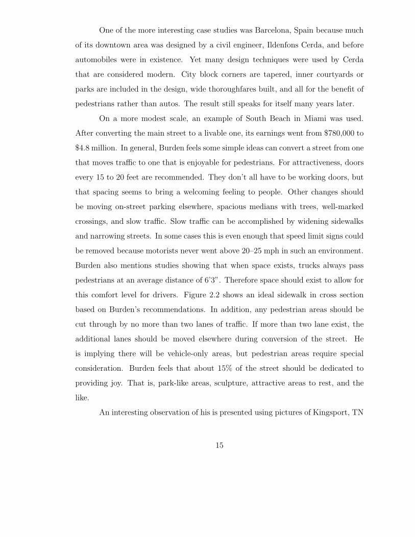
this comfort level for drivers. Figure 2.2 shows an ideal sidewalk in cross section

based on Burden’s recommendations. In addition, any pedestrian areas should be

cut through by no more than two lanes of traffic. If more than two lane exist, the

additional lanes should be moved elsewhere during conversion of the street. He

is implying there will be vehicle-only areas, but pedestrian areas require special

consideration. Burden feels that about 15% of the street should be dedicated to

providing joy. That is, park-like areas, sculpture, attractive areas to rest, and the

like.

An interesting observation of his is presented using pictures of Kingsport, TN

15

Bike lane

5’

Trees

5’

Walking

1−3’

Buffer Buildings, etc.

6−7’

Figure 2.2: Burden’s ideal sidewalk in cross-section.

which has very welcoming pedestrian areas that look perfect in all ways. However,

they were designed many decades ago. Burden gives his opinion that New Urbanism

is not new at all but re-use of old designs.

Burden’s discussion and presentation are exactly what is needed to help en-

gineers better understand the goals of community planning. His ideas are presented

clearly and illustrated with photos that strongly emphasize the points in ways words

often cannot. The main contribution from his work to simulator design is first mak-

ing the designer of the simulator aware of what interactions in the street are impor-

tant. The interactions can only be modeled in a detailed way if there is awareness

of how people affect others in the surrounding environment. Secondly, by making

the simulator designer aware of what works and what doesn’t regarding pedestrian

areas, the model can incorporate awareness of how the environment affects people.

The model is a simplification of reality that hopefully is close enough to the real

thing that it generates useful information. If realistic actions and values are not

designed into the simulator the output will be correspondingly unrealistic and of

limited value.

16

2.3.2 Behavior

Much of Whyte’s “City, Rediscovering the Center” [WH88] is devoted to

his detailed and frequent observation of pedestrians. Fruin’s [Fru71] landmark de-

tailed study of pedestrian behavior could also be useful in this area. Fruin’s work,

incidentally, is cited in a positive way by Whyte.

Whyte’s contribution is in studying the ordinary yet making unexpected dis-

coveries. The bulk of his study of pedestrian activity was accomplished by taking

photos and movies of people simply being themselves. While considering the social

life of the street, Whyte and his group of researchers spent five days at Saks Fifth

Avenue and Fiftieth Street in New York City and simply plotted the locations of

conversations lasting more than 2 minutes. What he expected to find is that when

people stop and begin a conversation that they would move out of the main flow of

pedestrian traffic. What he found was just the opposite. People prefer to continue

conversations while stopped in the midst of the heaviest traffic, he hypothesizes,

to remain uncommitted. Heavy traffic offers the possibility of breaking away or

not. In the case of the study mentioned above, the largest congregation of conversa-

tions took place at the street corner with a secondary concentration near the store’s

entrance.

Whyte also nicely describes the sorts of people a pedestrian might come upon.

Observing people’s reactions to street entertainers he writes:

It is interesting to watch people as they chance upon an entertainer.So often they will smile. A string quartet. Here at Forty-fourth! Theirsmile is like that of a child. For these moments they seem utterly atease, their shoulders relaxed. People enjoy programmed entertainment,too, but not in the same way. It is the unexpected that seems to delightthem most.

Whyte similarly gives descriptions of the handbill passers, prostitutes, muggers,

mentally ill, and other of the assorted array of characters encountered on the street.

17

Perhaps most interesting are his observations about the more typical pedes-

trian and how adept he is at maneuvering in crowds. He summarizes some chief

characteristics of the pedestrian in a list of eleven items. A couple examples of the

observations are that pedestrians form up in platoons at a light and will move in

platoons for a block or more, and pedestrians usually take the shortest cut. Even

when pedestrian malls outline curved tracks in the pavement, pedestrians ignore

them. They stick to the beeline.

Also useful are his observations about how transportation engineers treat the

pedestrian. Most would agree with his conclusion that pedestrian treatment is more

than a little lacking. Whyte brings up several examples. Among them, he points out

how the average pedestrian walking is not taken into account in traffic light timings.

Groups of pedestrians walk the length of a block then have to stop and wait for the

walk signal. They get to the end of the next block only to have to do the same

again. Engineers go to lengths to stop exactly this sort of stop and go pattern for

vehicles but rarely for those walking. Pedestrians have their own solution, Whyte

notes. They put themselves at risk and simply cross during the red.

He describes, too, how pedestrians tend to avoid collisions. The avoidance

begins at about 20 feet when eye contact is made. The two then usually begin

moving a half body width or so to one side; not enough to avoid the collision itself,

but is enough assuming the other person does the same. Collision avoidance between

pedestrians in streams at other angles are similarly described.

In addition to behavioral observations, effects of planning or lack of it are

discussed. He especially seems to like the mixture of businesses that zoning pre-

vents in the US. US zoning laws limit commercial areas to contain only certain

types of establishments, whereas streets in Tokyo are lined with an assortment of

random businesses sharing the area. The US cities approach, Whyte feels, lessens

the experience of the street.

18

Understanding how pedestrians behave is of paramount importance to the en-

gineer wanting to simulate the behavior. Whyte offers detailed observations about

behavior that can be built into a simulator. Coupled with Fruin’s detailed mea-

surements, these observations are perhaps of most immediate importance to any

pedestrian model. In order to realistically simulate pedestrian movement what is of

fundamental importance is little more than a detailed account of events encountered

by pedestrians and how they react to them. The work summarized provides much

of that.

2.3.3 Economic Value

Litman’s [Lit03] paper “Economic Value of Walkability” studies several as-

pects of the engineer’s perceptions, or rather misperceptions, of walking and how

valuable it is to society. In the broader sense walking is economically useful for

medical reasons. Killingsworth and Lamming [KL01] cite several conditions (whose

treatments are of course paid for by the health care system) that can be linked to

inadequate physical activity:

• Heart disease

• Hypertension

• Stroke

• Diabetes

• Obesity

• Osteoporosis

• Depression

• Some types of cancer

19

No one would claim increased pedestrian activity will eliminate these ailments, but

increased walking will certainly not diminish one’s health.

Litman’s paper, however, addresses more direct and easier to evaluate eco-

nomic impacts of increased walking. Studying data from other sources to determine

costs of walking versus driving, he looks at the various external costs including pub-

lic costs for road and parking facilities, traffic congestion, crash risk, and various

environmental impacts. Other modes also impose external costs, but usually at a

lower rate per trip. Walkability improvements that reduce automobile travel can

reduce these external costs. At the time of writing, savings by switching from driv-

ing to walking are estimated to be $0.25/mile under normal conditions and about

$0.50/mile during peak driving times.

Walkable designs also improve land use efficiency. Litman points out eco-

nomic, social, and environmental disadvantages of current development practices.

Only the economic issues are detailed here. Costs of current trends in development,

namely sprawl, are manifold. On Litman’s list are: reduced accessibility and higher

transportation costs, increased land devoted to roads and parking, increased public

services costs, reduced economies of agglomeration, reduced economies of scale in

transit and other alternative modes, threats to environmentally sensitive businesses

like farming and resorts.

He uses the definition of community livability to refer to the environmental

and social quality of an area as perceived by residents, employees, customers and

visitors. This encompasses issues related to health, safety, social possibilities, recre-

ation, aesthetics, and cultural resources. Litman references other work indicating

that while sidewalks have no effect on real estate value in auto dependent neighbor-

hoods, pedestrian friendly designs increase value of real estate. Similarly, nearness

to public trails and parks tends to increase both commercial and residential values.

20

He says, too, that while it is difficult to put dollar amounts on many of

these improvements, the increased community cohesion positively effects things such

as crime, equity, and diversion of some expenditures for auto upkeep to the local

economy.

Litman’s paper is difficult to directly incorporate into a model of pedestrian

behavior let alone into a simulator. However, after a simulator has proved its basic

predictions are reasonably accurate the next phase of simulator development is often

to have it generate analyses of scenarios. If economic viability of a design using work

like Litman’s could be used as part of the analysis, the output would be extremely

valuable. How possible it might be to incorporate such “fuzzy” ideas into an already

simplified model of reality is not clear, but should at least be considered.

2.3.4 Data Extraction

Once a model is implemented in a simulator, the model is tuned until its

actions seem appropriate. Further fine tuning is always needed, however, to make

the model match given real situations. This process is called calibration, and once a

model’s output closely duplicates known situations the model is said to be calibrated.

A model can only be calibrated if real world data has been extracted from observa-

tions. Observations of this sort are similar to Whyte’s [WH88] and Fruin’s [Fru71],

but require a higher level of detail.

Data extraction at this extreme level is far removed from the social science

aspects in many ways. However, data is not gathered for its own sake but must

represent events of interest to social science as well as events of economic interest.

Where, when, and why data is gathered must consider many of the behavioral

properties mentioned in previous sections. The “how” of collecting the data is

accomplished through purely technical means.

Hoogendoorn and Bovy [HB02, HDB03, Hoo03] address the technical con-

cerns of data extraction with the above considerations. They point out what is well

21

known to pedestrian simulator designers, that almost no detailed pedestrian data

is available. They set up experiments in areas such as commuter train stations and

have different groups of people wear differently colored hats. Other than wearing

these hats they were free to act as they wished. The pedestrian activity is filmed

from above as trains arrive and depart and people go their individual ways. The

researchers then generally follow a six step procedure:

1. Convert video to image sequences making radiometric corrections (adjusting

for changes in image intensity over time).

2. Identify probable pedestrian groups based on cap color.

3. Track detected pedestrians over duration of image sequence.

4. Map pedestrian tracks to a terrestrial coordinate system.

5. Use frame to frame directions to calculate likely pedestrian trajectories.

6. Present computer visualized trajectories.

The techniques used for most of the enumerated steps are highly mathemat-

ical. What is most important for this discussion is realization that an automatic

technique exists for converting some types of film footage of pedestrians into pedes-

trian trajectories changing over time. The results can be used to improve knowledge

of fundamental properties of walking allowing newer theories and models to be de-

veloped. Additionally, the data itself can be used for calibration of models.

2.3.5 Incorporating Behavior into a Model

Having studied pedestrian behavior for the ultimate purpose of simulating it,

the steps from data collection to theory or model are difficult because of variability in

behavior and the researcher’s ability to correctly recognize and identify cause-and-

effect. The papers “Modeling of Motorist-Pedestrian Interaction at Uncontrolled

22

Mid-block Crosswalks” by Sun et al. [SUBW03] and “Why People Cross Where

They Do” by Chu, Guttenplan, and Baltes [CGB03] are of interest because they

try to understand behavior and directly incorporate it into relatively simple models.

Both papers are based on extensive data collection.

In the case of Sun et al. [SUBW03], after data collection was complete they

developed several models that reflected the observations. As an aside, note that

while their model has the immediate goal of mimicking observed behavior, it has

important contributions to the area of pedestrian safety. In the National Highway

Traffic Safety Administration and Federal accident statistics [Kno75], study results

showed that 39% of urban crashes were pedestrian-motor vehicle accidents at mid-

block.

Sun’s group filmed a mid-block pedestrian crossing area over a period of 5

days at two times each day: peak vehicle volume (4:30–6:00pm) and peak pedestrian

volume (11:30am–1pm). The film was then carefully studied for two properties called

the Pedestrian Gap Acceptance and Motorist Yield. In the case of Pedestrian Gap

Acceptance the study concentrates on the gaps between vehicles. The gaps chosen

by pedestrians to use for crossing were studied statistically to learn their properties.

For instance, it was noted that individuals took an average of 4.6 seconds to cross

while groups of 2 to 4 took 5.6 seconds. Similarly, the Motorist Yield property of

driver behavior was studied. The idea behind it is simple. A motorist will either

yield or not yield for waiting pedestrians. The statistical results of the study allow

Sun to mathematically fit a function to the data. The function describes the data

well, but makes no effort to understand pedestrian motivation. The functions simply

describe the two properties of the data.

The case presented by Chu [Chu02] is slightly different. Unlike Sun, Chu

tries to understand why pedestrians act as they do. Chu’s group placed 86 volunteer

pedestrians at 48 locations on city blocks in Tampa Bay and asked where they would

23

cross. This not only helps model pedestrians better but in turn helps the planner

or designer know where, for instance, to place transit stops to make it more likely

that pedestrians will cross safely. The study attributes that pedestrians may trade-

off in making a choice are comfort, safety, time, and predictability. When asking

pedestrians where they would cross, they were given six choices:

1. Crossing at the left intersection (left intersection)

2. Crossing at a mid-block start point at a right angle (cross first and walk later)

3. Crossing with a jaywalk between the start and end points (jaywalk)

4. Walking on the near side to the opposite side of a mid-block end point and

crossing there at a right angle (walk first and cross later)

5. Crossing at the right intersection (right intersection)

6. Crossing at a mid-block crosswalk that is away from a start or end point

(mid-block crosswalk)

As with Sun, Chu’s group then used mathematical techniques to derive a function, a

nested logit model, that mimics the data. Typically used pedestrian level-of-service

tools make much simpler assumptions than Chu’s group. Chu’s group develops a

method that can describe using probability how and when pedestrians will cross a

street in an urban setting. The research additionally incorporates the behavioral

aspects of why the crossing place was chosen.

Both groups’ contribution to modeling is clear though the methods are dif-

ferent. Sun et al. show that behavior can be modeled without understanding of

its motivation. This makes it possible to describe or represent given conditions

but doesn’t offer much flexibility regarding effects of design changes in an area, like

Burden’s street treatments, i.e., conversion to pedestrian friendly designs, described

earlier. Chu et al. make the more important contribution showing that the behavior

24

can be modeled mathematically while being understood and described from a social

or behavioral standpoint. This important extra knowledge allows the modeler to

anticipate how design changes might affect pedestrian choices.

2.4 Engineering Models

When the point comes to implement a model of behavior, it means that first a

model must exist and that second it must be turned into software. Models are either

described using equations or algorithms. Though algorithms have more flexibility

it is exceedingly difficult to capture complex human behavior described in previous

sections in algorithms. That is why often the first step in modeling is to simplify

wherever possible. It is usually better to build up to a needed level of complex-

ity than to begin with an overly complex model. Currently, two software methods

of simulating pedestrians, and even vehicles, are exceedingly popular: cellular au-

tomata and agent based approaches. A cellular automaton (CA) has the attraction

of being easy to implement mainly because the geometry of movement is simpler,

but agent based modeling offers an approach naturally suited to modeling things

that think and move. Both methods will be described in more detail in coming

chapters since both are used in this thesis. Briefly, a CA is a grid of cells. Each cell

can be in one of several states, and a rule set is applied to each cell at every tick of

a clock. When the simulated clock ticks, the state of neighbors is used to modify

each cell’s state. An agent, on the other hand, senses and reacts to external stimuli.

Like all methods of problem solving, each has its strengths and weaknesses.

There are also many varieties of mathematical modeling approaches used. For

instance, a purely mathematical method making use of Markov models and queuing

theory is presented by Davis et al. [DDS03]. Based on existing data, the model

forecasts trends. While practical and useful, it does not take into account behavior

or model it, and so does not help with behavior modeling goals. Helbing [HFV00],

however, uses mathematics to characterize people’s actions in panic situations based

25

on their proximity to each other. The approach is similar in principle to agent based

modeling, though they do not use that term.

Hybrid approaches also exist. Toyama, Bazzan, and da Silva [TBdS06] use

agents in a CA framework so that different classes of agents can coexist. Typically,

pedestrian simulators uniformly model pedestrians. An impressive result of their

simulation is the spontaneous formation of lanes in large open areas.

2.4.1 Cellular Automata

Nagel and Schrekenberg [NS92] present a cellular automaton model of high-

way traffic flow that is similar in nature to the more involved multi-agent model of

the same [WS01]. The rule set will be presented and discussed in the next chapter.

However, this same rule set was applied to pedestrian environment by Blue [BA98]

with limited results. This is perhaps not surprising because pedestrians don’t pass

each other in the same way that cars do, nor follow each other in lane-like forma-

tions. The disappointing results show just how important the cellular automaton

rules are. Because many, many cells abide by identical rules, the tiniest of changes

in the rules has wide ranging effects on the ultimate system organization. The re-

sultant system-wide behavior resulting from behavior at the individual level is often

called emergent behavior.

Yamamotoa et al. [YKN07] offer a set of four simple rules to model general

pedestrian movement which matches well several evacuation situations. In [MN00],

Muramatsu and Nagatani simulate jamming in pedestrian traffic. Blue and Adler

[BA01] model bi-directional walkways, as do Li, Yang, and Zhao [LYZ05]. Perez

et al. [PTLS02] use a CA to model confined pedestrians. Kretz and Schreken-

berg [KS06] compare the development of CA rules using von Neumann and Moore

neighborhoods. Von Neumann neighborhoods are made of cells laterally adjacent

while Moore includes both laterally and diagonally adjacent cells. In all cases, the

26

researchers use CA rules that can reasonably model their particular situations of

interest.

CAs tend to be most appropriate for expansive simulations studying emer-

gent behavior of thousands of agents. In such large scenarios behavior of individuals

is not apparent and so a single rule set is appropriate. At more detailed levels of

simulation where interest is in the range of dozens to hundreds of individuals, de-

tailed behavioral characteristics have more of an effect and are not averaged away by

huge numbers. Modeling of individual characteristics is where agent based modeling

excels in comparison to cellular automata.

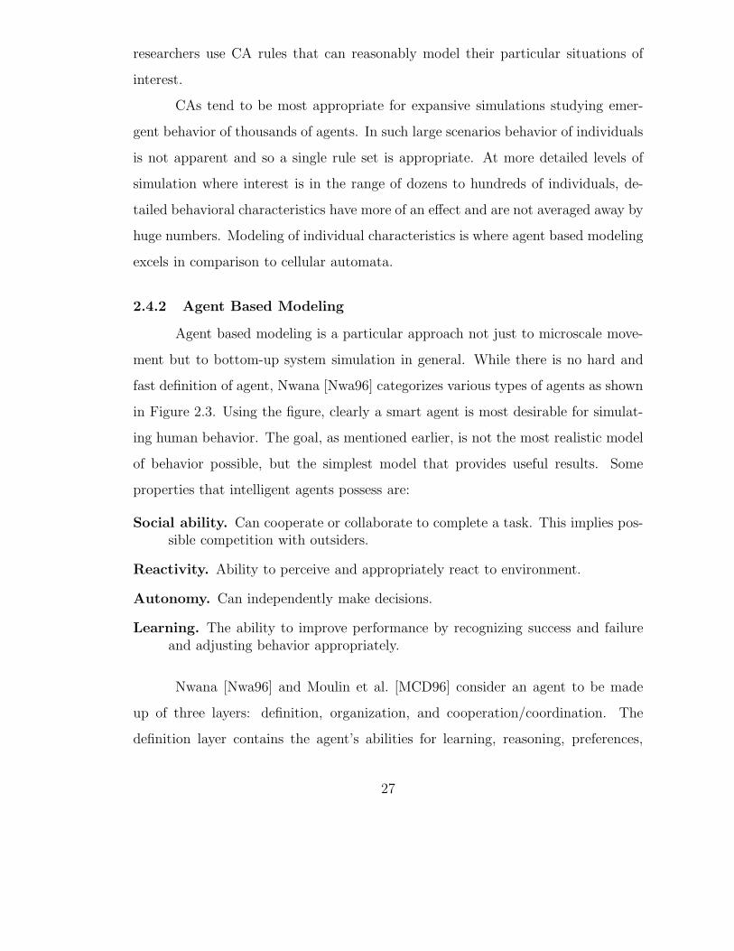
2.4.2 Agent Based Modeling

Agent based modeling is a particular approach not just to microscale move-

ment but to bottom-up system simulation in general. While there is no hard and

fast definition of agent, Nwana [Nwa96] categorizes various types of agents as shown

in Figure 2.3. Using the figure, clearly a smart agent is most desirable for simulat-

ing human behavior. The goal, as mentioned earlier, is not the most realistic model

of behavior possible, but the simplest model that provides useful results. Some

properties that intelligent agents possess are:

Social ability. Can cooperate or collaborate to complete a task. This implies pos-sible competition with outsiders.

Reactivity. Ability to perceive and appropriately react to environment.

Autonomy. Can independently make decisions.

Learning. The ability to improve performance by recognizing success and failureand adjusting behavior appropriately.

Nwana [Nwa96] and Moulin et al. [MCD96] consider an agent to be made

up of three layers: definition, organization, and cooperation/coordination. The

definition layer contains the agent’s abilities for learning, reasoning, preferences,

27

Interface

Autonomous

LearnCooperate

Smart

Learning

Collaboration

Collaboration

Figure 2.3: Types of software agents.

and goal finding. The organization layer contains the agent’s relationship to other

agents. And within the coordination layer exist the agent’s social abilities. In the

context of transportation systems, the agent will be either a pedestrian or a vehicle.

Engineers and scientists usually tailor software to implement their models.

An interesting package, SWARM [Ins08], is developed by the Sante Fe Institute

that is a tool kit developers can use to create a variety of agent based models.

The SWARM Development Group realized that agent based simulation is a general

method of simulating systems. As such, they decided rather than having researchers

around the world address their own simulations on a case by case basis, a general

tool should be developed that can be used to solve many simulation problems in

much the same way that computer programming languages are used. SWARM of-

fers useful constructs like Java language libraries. This makes it possible to program

28

arbitrary agent based systems. Because many details of an implementation are still

left up to the programmer, most developers still choose to write their own simu-

lators from scratch. This is especially true in transportation simulations because

the SWARM library does not incorporate methods for spatial modeling of agents, a

major component of transportation modeling.

A popular agent based system that can be applied to pedestrian traffic flow

is the Ant System. The Ant System [BDT99] mimics ants in a simple way. When

ants walk, they leave a chemical trail behind them. As they randomly explore and

happen across food, they follow the chemical trail back to the colony depositing

more chemical as they walk. As more ants find and use this trail more chemical

scent is deposited. The stronger the scent, the more likely that an ant will follow

the trail. In this way, a pedestrian simulation can have pedestrians randomly try to

find the best route between two points. As different pedestrian agents happen upon

better and better routes, more people will follow them. An analogy can be drawn

to people walking in the snow. It’s easier to follow existing footprints than it is to

strike out on your own.

PEDFLOW [WKHK00] is an agent based simulator that allows rules of move-

ment to be defined by the modeler in a flexible manner. Each PEDFLOW pedestrian

makes decisions based on how it’s neighbors are moving. The difficulty is determin-

ing exactly what the rules should be. The work of Daamen [DH03, Daa02] could

be helpful in rule development, i.e., behavior description, because her work starts

by studying people. A large experiment was carried so that microscopic pedestrian

data could be acquired. Here, microscopic means movement details at a low level. A

mathematical model of pedestrian movement is then built up from the experimental

results. The mathematical model captures the side effects of human behavior but

doesn’t try to model it directly.

29

For example, in one PEDFLOW effort by Kula et al. [KKWH98], both pedes-

trians and buildings are modeled as agents. While buildings in reality are inanimate,

in PEDFLOW they are not. As pedestrian agents wander near building agents, the

building “calls out” to the pedestrian requesting attention. Depending on the pedes-

trian’s own interest level, it might approach the building more closely. Pedestrians

in the scenario modeled are hindered by a building blocking their way. Eventually,

the AI (artificial intelligence) rules used by each agent allow them to find a path

around the building first by trial and error, and later by simply following other

agents.

In [Jia98], Jiang also models pedestrians through the use of a multi-agent

system named SIMPED. In the SIMPED environment are museums and shops,

and pedestrians are goal-oriented. They all are headed to a particular place. In

this regard, SIMPED and PEDFLOW are quite similar. SIMPED also incorporates

more elaborate path finding in an urban environment. The pedestrians must traverse

several irregularly shaped city blocks to reach their destinations. Therefore, they

are required to roughly map out their routes and refine their route as they travel.

Some amount of communication occurs between agents. (Communication between a

building and a pedestrian amounts to giving information to the simulated pedestrian

that he can’t walk through it, that it is so wide, perhaps a corner building, etc.)

2.5 Summary

As one would expect, each type of model performs well in the niche it was

designed for. The very nature of simulators, that they are simplifications of reality,

means results can never be exactly what one will see in the real world. However, an

engineer’s goal of getting answers that are good enough to get the job done should

be realizable in the case of modeling pedestrian movement. The literature surveyed

offer important and useful information making use of social science concerns and

observations or offer techniques of use to the engineer building a model. Modeling

30

is not established well enough to incorporate complex human behavior, yet models

of pedestrian movement can only be reasonably accurate if some awareness of social

science observations are included. Certainly some of the observations can be mod-

eled, and the major goal of the literature survey has been to become aware of these

observations and ideas that can contribute positively to the development of better

and more realistic pedestrian behavior models.

There are many simulators for both vehicle and pedestrian movement, how-

ever the ones presented are fairly representative of the current state of the art. It is

noteworthy that in the models presented that pedestrians view other pedestrians as

obstacles or, in some cases, sources of information. There is no social awareness or

consideration of them as family or friend. That means in smaller scale simulations

there are no effects based on the normal social grouping of people.

31

Chapter 3

VEHICULAR MOVEMENT SIMULATION

3.1 Introduction

Simulating vehicular movement requires first deciding which behavior is im-

portant. When designing a small, narrow bridge, for instance, drivers’ natural ten-

dencies to sway away from the roadway edge towards the center line is important.

But in general situations, vehicular lateral movement is not. Similarly, for an initial

effort at modeling vehicle interactions, it is appealing to start with a simple model

and add to it until it offers the desired level of resolution.

The most important of the original vehicle models is the GM Car Following

Model developed in 1959 [DCG59] and gradually enhanced over the decades. The

model is often presented using Newton’s “dot” notation to indicate a derivative

rather than Leibniz’s more commonly used dy/dx notation:

..xn+1 (t + ∆t) = α(l, m)

.x

m

n+1 (t + ∆t)

(xn(t)− xn+1(t))l[

.xn (t)−

.xn+1 (t)] (3.1)

At first glance the notation is somewhat opaque, but a few words make the model

clear. The argument t is some arbitrary point in time, and t + ∆t is an instant

later when a driver begins to react to a stimulus. Subscripts n and n + 1 refer

to two vehicles, lead vehicle n and following vehicle n + 1. Their positions, or

rather, distances from some arbitrary point, are xn and xn+1; speeds are indicated by

appropriately subscripted.x; and accelerations by

..x. With just this much description

it is apparent that the model defines the following vehicle’s acceleration as a reaction

32

to the relative speed of the vehicles, as indicated by the term in brackets. This is the

so-called stimulus term; it stimulates a change in the follower’s speed. The leading

portion before the brackets is the sensitivity term and controls how aggressively the

model responds to the stimulus. The method of determining values for exponents l

and m, and for constant α is interesting but not necessary to detail here.

The mathematics includes implicit assumptions. For instance, it assumes

the response is dependent only on the stimulus and that relative speed is the only

stimulus. The nature of differential equations is that steady state is also implied. As

a result, the GM model is useful for free flowing traffic but not, say, for intersection

studies.

Nagel and Schrekenberg [NS92], as mentioned in the last chapter, approached

the problem from a different viewpoint. Rather than describe the system as a whole,

they put their efforts into describing a single vehicle and how it reacts to neighboring

vehicles. Their model consists of a set of simple rules that are evaluated in the

context of a cellular automaton [vNB66], or CA. A CA is a discrete model that in

the two-dimensional case is a grid of cells whose grid size is set by the modeler.

Each cell in the grid can be in one of a finite number of states, again determined by

the modeler. At each tick of the clock, each cell simultaneously monitors the state

of its neighbors, and then updates its own state based on what state neighbors were

in. In the GM model, comparison were made between times t and t + ∆t, and the

same is true here except that ∆t is always one time unit.

A famous example is John Conway’s “Game of Life” CA [Gar70]. Each cell

in the grid is in one of two states, alive or dead. When the clock ticks, every cell

makes the following state transitions:

1. If alive and has less than 2 living neighbors, cell dies (lonely).

2. If alive and has more than 3 live neighbors, cell dies (overcrowded).

33

3. If alive and has 2 or 3 live neighbors, no change (healthy).

4. If dead and has 3 neighbors, cell comes to life (birth).

It is difficult to predict how a system will evolve from a random starting pattern, and

this is what makes CAs so interesting and powerful. The system evolves and displays

an emerging behavior probably not predictable initially. It clearly requires computer

simulation, however, to generate results whereas partial differential equations are

pleasing because they concisely and elegantly describe an entire system.

In the case of Nagel and Schrekenberg, they developed three rules equally

simple as Game of Life’s that describe traffic flow in one lane. The lattice in their

CA represent road positions that can accommodate a single vehicle. Each cell is one

of two states, vehicle or empty, and state transitions are:

1. Acceleration: s(t + 1) = min(s(t) + 1, smax, g(t))

2. Deceleration: s(t + 1) = max(s(t)− 1, 0), with probability r

3. Speed: p(t + 1) = p(t) + s(t)

where s(t) represents a vehicle’s speed in cells per time step at time t, g represents

the gap length in units of cells between the vehicle and the one it follows, and p is the

cell name, i.e., its number or position, that will next contain the vehicle currently

in this cell. Notice the realistic movement and minor congestion build up illustrated

in Figure 3.1.

3.2 Model

The obvious limitation with the model is that there is one lane. It can

be extended to multiple lanes in the obvious way, but only if the constraint of

no lane changing is acceptable. Since lane changing is used to avoid congestion

and, inadvertently, to create it, extending the model to incorporate lane changing

34

5

Speed in cells/time step

5 4 35

4 1 4

4 1 3

Direction of Travel

Time

Figure 3.1: Nagel and Schrekenberg vehicular CA.

35

is worthwhile. Because the resultant simulation will be more realistic, the results

will be more reliable. The remainder of the chapter is devoted to extending the

model, implementing it in a simulator, and evaluating the results. This work was

presented at an ad hoc session on artificial intelligence and simulations at the 2003

Transportation Research Board.

3.2.1 Lane Changing

The greatest difficulty in developing CA rules for lane changing is that lane

changes are made based on current position relative to destination. In a free flow

condition, lane changing is made only due to a speed increase incentive. But as

the destination more and more closely approached, the speed incentive steadily

decreases.

First, we consider the free flow situation since it is the easier of the two. In

this case, there are potentially three gaps that offer different speeds: the gap ahead,

the one to the left, and the other to the right. Assuming a safe driver, the new gap

left behind after a lane change must also be considered to allow a new follower safe

braking distance. Free flow lane change is then described as follows. Equations for

gap ahead and gap behind are, respectively,

ga(t) = xn(t)− xn+1(t) (3.2)

gb(t) = xn−1(t)− xn(t) (3.3)

where xi is a vehicle position or distance as defined in Equation 3.1, the GM Car

Following Model. A vehicle’s new speed after a potential lane change is given by

sl(t + 1) =

0 if gb(t) < s(t)

0 if ga(t) < s(t) + 1

min(s(t) + 1, qsmax) otherwise

(3.4)

where subscript l is -1, 0, or 1, indicating attainable speed in, respectively, the lane

to the left, the current lane, or to the right of the current lane. The reason for scaling

36

the maximum speed by q is described below. All functions yield results relative to

the lane of interest. The first line indicates that a move to the lane of interest would

yield a speed of zero because there is inadequate space between the potential new

position and the following vehicle. The second line says the same about leaving safe

following distance ahead, but also with the “+1” indicates that there is no value in

a lane change unless speed increases. If safe space is left behind and ahead, then the

third condition holds and indicates what the new speed would be. The new vehicle

speed is then given by

v(t + 1) = max(s−1(t + 1), s0(t + 1), s1(t + 1)) (3.5)

The function sl(t) only yields new speed and not new lane. That is the

subject of the next equation. Here, f(t + 1) returns -1, 0, or 1, indicating whether

the vehicle of interest will, respectively, move to the left of, remain in, or to the

right of the current lane. The new lane taken by the vehicle is then

f(t + 1) =

−1 if s−1(t + 1) > s(t)

1 if s1(t + 1) > s(t)

0 otherwise

(3.6)

Note that the order of consideration implies a tendency to move to the left before

moving to the right for a lane change.

The second and more general case deals with the situation when a vehicle

nears a destination. The situation is akin to the dilemma zone encountered if traffic

lights are improperly timed for the posted speed limit. No matter what the speed

incentive for a lane change, a driver will not change lanes when reaching the desti-

nation is imminent. The extremes are imminent arrival and locations well beyond

where navigation toward the destination is needed. In between the extremes, how-

ever, different behaviors are exhibited. The aggressive driver takes large risk for

37

little gain. This type of personality might pass a slow vehicle even when the desti-

nation is not far. Conversely, a conservative driver will stay put even if there is a

comfortable amount of time for a lane change to overtake a slow vehicle.

This is modeled by taking a radius r, beyond which there is no need for

consideration of moving towards destination. Within a distance of r, however, the

vehicle will be at an instantaneous position p. The conditions in the preceding

equations, are now augmented to use probability rather than determinism. When

r = p, then p/r = 1. At the destination, p = 0 and so p/r = 0. It is natural to

use q = min(1, p/r) as a scale factor for the maximum speed, as shown above in

Equation 3.4.

3.2.2 Reaching the Destination

The addition of probabilities to allowing lane changing is also used to control

navigation towards the destination. When for whatever reason a vehicle is not in

the proper lane to reach its destination, the closer it approaches the destination,

the more likely it must move towards it. Using the same decision threshold radius

r, now we consider the distance based probability q = min(1, p/r). As above, this

probability q is 1 at a great distance, i.e., beyond a distance of r, and is 0 at the

destination. If d is the direction of the destination lane, where -1 is a lane somewhere

to the left, 0 is current lane, and 1 is a lane somewhere to the right, then the new

lane taken by the vehicle to move towards the destination is

n(t + 1) =

−1 if d < 0

1 if d > 0

0 otherwise.

(3.7)

which reduces to the more concise

n(t + 1) = d (3.8)

38

The final consideration dealing with lane change is whether to use f(t + 1) which

allows overtaking slow movers, or to use n(t + 1) which moves a vehicle towards

its destination lane. The decision would be difficult if they generated competing

probabilities, so they must be made cooperative by making a vehicle less likely to

change lanes as it nears its destination and is in the wrong lane. Here, scale factor

q is used to decrease the maximum speed in each non-destination lane. The idea is

that as the destination is closely approached, the maximum speed available in the

other lanes gets closer to zero. Speed advantage is greatest in the destination lane.

Beyond the distance threshold r, however, the scale factor q is one and has no effect.

Or, when f(t + 1) 6= n(t + 1),

l(t + 1) =

f(t + 1) with probability q

n(t + 1) with probability 1− q(3.9)

3.2.3 Dealing with Interference

The final consideration in lane changing is handling decisions when plans

can’t be met. In the preceding section, two distance based probabilities were used,

p/r and 1 − p/r. The probability thresholds approach 0 and 1 in either direction,

but based on the random number chosen as the probabilistic experiment the wrong

decision can be repeatedly made. It is possible, for instance, for a vehicle to more

and more closely approach its destination yet continue to choose to either move

away from the destination, not move towards it, or even choose to do either but

be prevented due to congestion. From the rules presented to this point, in such a

situation a vehicle in the wrong lane would reach a fork in the road and simply stop;

neither realistic nor beneficial to the system!

The final of the three rules offered as additions to the Nagel Schrekenberg

rule set can be stated in words as, if in the wrong lane and can’t reach destination

lane, then take the wrong way. This mimics the unenjoyable situation sometimes

39

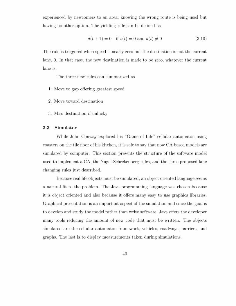
experienced by newcomers to an area; knowing the wrong route is being used but

having no other option. The yielding rule can be defined as

d(t + 1) = 0 if s(t) = 0 and d(t) 6= 0 (3.10)

The rule is triggered when speed is nearly zero but the destination is not the current

lane, 0. In that case, the new destination is made to be zero, whatever the current

lane is.

The three new rules can summarized as

1. Move to gap offering greatest speed

2. Move toward destination

3. Miss destination if unlucky

3.3 Simulator

While John Conway explored his “Game of Life” cellular automaton using

coasters on the tile floor of his kitchen, it is safe to say that now CA based models are

simulated by computer. This section presents the structure of the software model

used to implement a CA, the Nagel-Schrekenberg rules, and the three proposed lane

changing rules just described.

Because real life objects must be simulated, an object oriented language seems

a natural fit to the problem. The Java programming language was chosen because

it is object oriented and also because it offers many easy to use graphics libraries.

Graphical presentation is an important aspect of the simulation and since the goal is

to develop and study the model rather than write software, Java offers the developer

many tools reducing the amount of new code that must be written. The objects

simulated are the cellular automaton framework, vehicles, roadways, barriers, and

graphs. The last is to display measurements taken during simulations.

40

Figure 3.2: Center lane and edge lane cell connectivity.

3.3.1 Roadway Cell and Barrier

A roadway cell represents the amount of space that one vehicle takes up.

It can be in one of two states, has vehicle or has no vehicle. In addition, it has

a speed limit and connectivity information. The simulations are two dimensional,

but by using speed limits on a per cell basis it is possible to simulate slowing on

crests or due to construction. Because a CA evolves in time based on grid neighbor

states, a cell also includes its connectivity data. In the middle of a roadway, cells

are connected to all neighbors, meaning that a vehicle can potentially move to any

of its nearby cells. At road edges or at a split in a road, there is no connectivity to

adjacent cells, as shown in Figure 3.2. While such barriers are so obvious to humans

that they are reacted to nearly subconsciously, their explicit existence is critical to

proper simulation.

In the real world a barrier is an obstacle while in the simulator a barrier is

lack of connectivity. When the CA simultaneously executes its rule set on all cells,

state change is based on neighbor states. Each neighbor’s state, however, can only

be observed when there is connectivity. For example, a back up on an exit ramp

41

parallel to a road will have no effect on the roadway flow.

When the roadway is drawn on the screen, if a cell edge has no connectivity

then that edge is drawn with a thick black line. The connectivity information is

communicated in a visually expected way. The simulator is aware of the lack of

connectivity and the human observer sees an obstacle as expected by real world

experience.

3.3.2 Vehicle

A vehicle is more easily modeled. It is characterized by color, maximum

attainable speed, and destination lane. Maximum speed feeds into the CA rules

detailed in Equation 3.4. Due to speed limiting, a vehicle might not be able to

realize its potentially maximum speed. That is, speed at time t is

s′(t + 1) = min(cmax, v(t + 1))

where cmax is a cell’s upper speed limit and v(t + 1) is the vehicle’s new speed as

determined by Equation 3.4.

The destination lane also is used by the lane changing CA rules in Equa-

tions 3.7 through 3.10. Vehicle color is clearly for the sake of human observers

of the simulation. It is useful to sometimes color code by destination to observe

weaving, or by origin to observe lane changing and sources of congestion.

3.3.3 Cellular Automaton

To make use of the objects described to this point, the cellular automaton

simulator itself must be implemented. It is aware of the grid, which is the user

defined organization of cells that make up the roadway surface, and is aware of

cell state which includes vehicle state of the cell happens to contain one. Most

importantly, it maintains the simulation clock and applies the rule set to each cell

at each tick of that clock.

42

There is other code, possibly exceeding in size the core simulator objects, that

is used to animate the simulation, allow communication between objects, and handle

interactive user editing of scenario set ups. While complex in its own right, the code

is uninteresting from the standpoint of the model and is not further elaborated upon

in this work with the exception of on-screen data plots.

3.3.4 Graph

Data plotting is handled by a special object dedicated to the task. There

are two types of graphs commonly used to summarize vehicular traffic properties:

standard data point plotting and scrolling time-distance plots. Of the first type, it is

the three fundamental curves of highway traffic stream characteristics that are most

often plotted, as presented in, for instance, [PP01] and [WA98]. The fundamental

relationship used is

q = ku (3.11)

where

q = volume, vehicles/hr

k = density, vehicles/km

u = speed, km/hr

Given density k and speed u(k), flow q is defined as their product. The model for

u(k) is based on safe car following expectations, and as such can vary somewhat

based on assumptions built into the model. By studying three curves obtained by

graphing each of u, k, and q against each other, predictions can be made regarding

shock wave dissipation, expected speeds, and so on. The references cited provide

a wealth of detail summarized in brief here. In theory the curves look like those

of Figure 3.3, so any simulation results must look very similar. In the figure, the

variables are qmax, the maximum volume achieved; um, the speed at qmax; km, density

at qmax; and kj , the density at which jamming occurs.

43

qq

u

u

m

max

k

jkmk

mu

u

q

qmax

km kj

k

Figure 3.3: Traffic flow curves.

44

The second type of curves needed, time-distance plots, are used to view the

history of traffic moving on a roadway. Examples can be seen in Results, section 3.4.

At fixed intervals in time, the positions of vehicles are plotted relative to some point.

If a vehicle were to maintain a steady speed, the resultant plot would be a straight

line. When traffic is heavier, vehicles tend to increase and decrease speed based

on conditions, though, and so instead of straight lines, one sees waving lines that

should never touch. Any that touch indicates a collision.

Figure 3.4 shows the history of two platoons. The first platoon is made up

of six vehicles whose first vehicle maintains a steady speed throughout the trace.

The second vehicle, however, suddenly slows down at one point only to soon after

over-compensate and speed up. Finally, at the end of the S-shaped segment it slows

down its original speed. The third, fourth, and fifth vehicles respond in a similar

way, but their responses are more and more attenuated because they are able to

react more quickly when they overtake each of their lead vehicles. The response by

the fifth vehicle is such a damped version of the first that the sixth vehicle required

no change in speed. At some distance behind the first platoon is a second platoon

of two vehicles whose accelerations were also zero throughout.

While watching a simulation offers an intuitive feel for whether the vehicle

responses are accurate or not, the data plots offer complete histories that can be

compared against real data.

3.4 Results

Among the first simulator results to be checked are the plots of data points

making up the three fundamental curves. It is important to note that the simulator

plots measured data only. There is no built-in knowledge of the three fundamental

traffic flow curves which is used to somehow control or affect the simulation. The

simulation proceeds completely based on the six rules previously detailed. At each

time step, in addition to applying the rule set to each cell in the CA, measurements

45

last inplatoon

lead

last

time

leadvehicle

distance

Figure 3.4: Time-distance curve.

46

Figure 3.5: Traffic flow curves from simulation.

are taken of each cell whose state indicates that it contains a vehicle. As traffic

density is increased from zero to 100%, Figure 3.5 shows the results. See how

closely they resemble the purely theoretical curves of Figure 3.3. Immediately, we

begin to trust the results of the simulator because of this correlation. The k-u, k-q,

q-u curves capture behavior, and the similarities between mathematical model and

simulation display similar behavior. Other studies have compared the model with

real data and have shown similar closeness which is why the curves are relied upon.

There is no need to compare time-distance curves between model and theory

because there is no theoretical equivalent of the derivation of the fundamental curves.

A time-distance plot is simply a measurement that concisely displays roadway travel

history, whether the history is real or simulated. So with justification for trust in

the model, individual situations can be considered.

3.4.1 Weaving

Nagel and Schrekenberg studied their three rules extensively, so the reader is

referred to their papers for in-depth studies and analyses of those three rules. Our

interest is in the effects of the additional three rules supporting lane changing, and

weaving is of foremost interest in that regard. The name weaving aptly describes

47

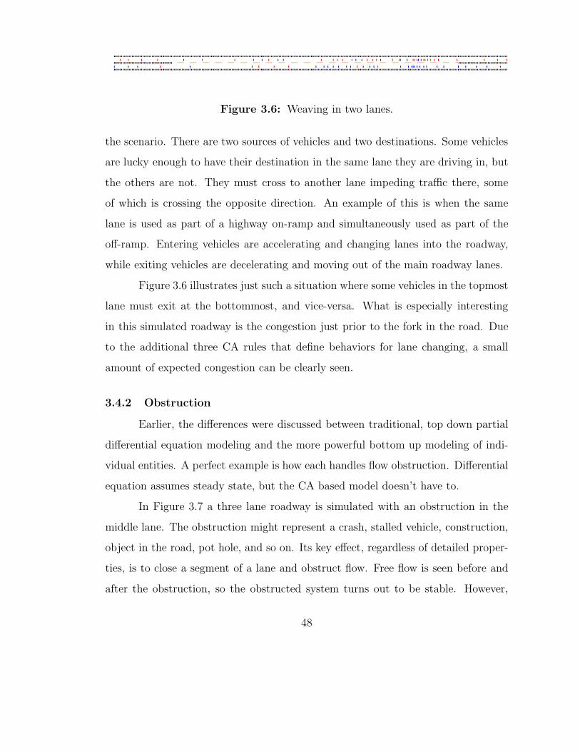
Figure 3.6: Weaving in two lanes.

the scenario. There are two sources of vehicles and two destinations. Some vehicles

are lucky enough to have their destination in the same lane they are driving in, but

the others are not. They must cross to another lane impeding traffic there, some

of which is crossing the opposite direction. An example of this is when the same

lane is used as part of a highway on-ramp and simultaneously used as part of the

off-ramp. Entering vehicles are accelerating and changing lanes into the roadway,

while exiting vehicles are decelerating and moving out of the main roadway lanes.

Figure 3.6 illustrates just such a situation where some vehicles in the topmost

lane must exit at the bottommost, and vice-versa. What is especially interesting

in this simulated roadway is the congestion just prior to the fork in the road. Due

to the additional three CA rules that define behaviors for lane changing, a small

amount of expected congestion can be clearly seen.

3.4.2 Obstruction

Earlier, the differences were discussed between traditional, top down partial

differential equation modeling and the more powerful bottom up modeling of indi-

vidual entities. A perfect example is how each handles flow obstruction. Differential

equation assumes steady state, but the CA based model doesn’t have to.

In Figure 3.7 a three lane roadway is simulated with an obstruction in the

middle lane. The obstruction might represent a crash, stalled vehicle, construction,

object in the road, pot hole, and so on. Its key effect, regardless of detailed proper-

ties, is to close a segment of a lane and obstruct flow. Free flow is seen before and

after the obstruction, so the obstructed system turns out to be stable. However,

48

Figure 3.7: Lane obstruction.

Figure 3.8: Simulated on-ramp.

and as expected, there is considerable congestion prior to the blockage. The close

spacing shows how slowly the vehicles are traveling because the CA rules model safe

driving behavior. That is, there is no tailgating at high speed, so the simulated

results are likely to be a somewhat conservative.

3.4.3 On-ramp

Figure 3.8 represents an on-ramp merging with a highway. Notice that the

simulation uses connectivity information to both separate the on-ramp from the

rest of the lanes making up the road, and also to come to an end after some length.

Graphical presentation does not affect the model. Even though real on-ramps merge

smoothly and do not abruptly come to an end, the CA rule set works identically

regardless of how the scenario is drawn on the screen. At some point, there is no

more room for a vehicle in the on-ramp lane. Because the rule set has each vehicle

look ahead some distance, the vehicles are aware of when they must begin to move

out of the on-ramp lane.

The example of Figure 3.8 is what every transportation engineer hopes to

49

Figure 3.9: Complex highway.

see. A fully utilized road without congestion and which allows entering vehicles

easy merging. The only hint of congestion is where one would expect to see it; at

the start of the on-ramp where speed is slowest.

3.4.4 Complex

In addition to the simulated features described to this point, there are often

roadway properties that cause a driver to slow down. Crests, valleys, and curves are

common examples. Figure 3.9 simulates a portion of roadway where many things

conspire to produce a congested stretch of road. Traffic moves from left to right,

and notice that the first thing out of the ordinary encountered by vehicles is a light

gray rectangle spanning a small portion of all four lanes (to the left of the small,

darker box). The darker the shade of gray, the lower is the permitted maximum

speed. In this case it might simulate cars slowing as they reach the crest of a hill

only to immediately discover that there is an obstruction in the second lane from

the left, that is, the small, dark box with no surrounding connectivity. Once past

the obstruction the road splits three ways causing weaving of vehicles between the

four lanes increasing congestion still more.

3.5 Analysis

The new contribution of the rule set is ability to simulate lane changing.

Anuj Gupta, a master’s student in civil engineering, assisted with additional studies

50

0

0.1

0.2

0.3

0.4

0.5

0.6

0.7

0.8

0.9

1

0 0.1 0.2 0.3 0.4 0.5 0.6 0.7 0.8 0.9 1

Nor

mal

ized

Num

ber

ofLan

eC

han

ges

Normalized Density, k

AggressivePassive

Figure 3.10: Lane changing vs. density.

focused on lane changing. He studied two types of drivers, aggressive and passive,

which were modeled by modifying the lane changing rules slightly. The probabilities

for lane change were increased to simulate drivers aggressively changing lanes, and

lower probabilities to simulate safer, more passive drivers who change lanes less fre-

quently. Figure 3.10 shows the results. The two curves can be clearly distinguished

form each other, but both peak at about the same point. It demonstrates that

regardless of behavior, increased congestion constrains and ultimately prevents lane

changing. Conversely, at low densities there is less lane changing because there is

little traffic and hence little motivation.

In Figure 3.11 a third behavior is added, that of no lane changing. What is

interesting to note is that the aggressive drivers actually reduce flow for the entire

system, because their additional movements cause disturbances. Lane changing

becomes progressively more difficult at higher densities, so the effect of aggressive

driving is reduced. As interesting, some amount of passive lane changing increases

51

0

0.2

0.4

0.6

0.8

1

0 0.2 0.4 0.6 0.8 1

Nor

mal

ized

Flo

w,q

Normalized Density, k

AggressivePassive

No lane change

Figure 3.11: Flow vs. density.

flow.

Density increases from bottom to top in Figure 3.12 and so the lane changing

maximum is now to the right. Travel time is defined as the length of time required to

travel the length of roadway studied. It is normalized here so that the longest travel

time experienced is 1. Normalized data is more easily calibrated. In the graph, travel

time quickly increases after the point of maximum lane change. Higher density, as

expected, reduces the opportunity for lane changing and in general increases travel

time.

Finally, Figure 3.13 shows that despite a large change in lane changing rate,

there is not a correspondingly large variation in flow. The symbols on each curve

indicate, as in Figure 3.12, density increasing from 0 to 1. As also seen in the other

plots, when density increases lane changing also increases to some maximum for

each behavior, and then decreases due to congestion.

52

0

0.1

0.2

0.3

0.4

0.5

0.6

0.7

0.8

0.9

1

0 0.1 0.2 0.3 0.4 0.5 0.6 0.7 0.8 0.9 1

Nor

mal

ized

Tra

velT

ime

Normalized Number of Lane Changes

Density

Figure 3.12: Travel time vs. lane changes.

0

0.1

0.2

0.3

0.4

0.5

0.6

0.7

0.8

0.9

1

0.1 0.2 0.3 0.4 0.5 0.6 0.7 0.8 0.9 1

Nor

mal

ized

Lan

eC

han

geR

ate

Normalized Flow, q

AggressivePassive

Figure 3.13: Lane changing vs. flow.

53

3.6 Summary

Extensive studies have shown that the three fundamental traffic flow curves,

as derived mathematically, are reasonable models for real traffic behavior. Nagel

and Schrekenberg demonstrated that their three rules offered a close approximation

to the fundamental curves, enough that their CA results could be relied upon to

predict traffic patterns. After the addition of three additional rules that support

lane changing, we similarly showed via simulator measurements that our new rules

continue to create a system whose behavior mimics that shown by the fundamental

flow curves. Additional studies of isolated examples including obstacles, weaving,

and speed limiting continued to demonstrate expected results, and the graphical

display, whose images are presented in this chapter, offer intuitive verification.

Further studies by Gupta considered the effects of the new lane changing

rules. The scenarios showed how aggressive driving can decrease system through-

put. Furthermore, lane changing has little effect in increased congestion simply

because lane changing becomes difficult to accomplish. Similarly, in light traffic

lane changing has little effect because it is not necessary in low density, low volume

situations.

There is room for future work and extensions. While our new rules allow

vehicles to pass slower vehicles and to do so with a preference to pass on the left,

there is no rule urging a passing driver to return to its lane of origin after completing

the pass.

Further area for improvement lies in the rule that increases a driver’s likeli-

hood to move toward its destination lane. At the moment, the probability is based

completely on distance to the fork in the road. It should also be based on how many

lanes distant it is from the destination lane. For multi-lane highways, this probably

can add to the correctness of results.

The cell connectivity modeling also creates limitations that can be removed.

54

When adjacent cells are not connected, as in the case of on ramps, off ramps, and

divergences in roadways, the CA models absolute disconnectedness. This prevents

modeling of the gawking, or “rubber necking,” factor which has a significant impact

on flow.

While research always can be carried forward further, the model and results

presented show that a CA with six simple rules can offer the transportation engineer

an extremely useful predictive tool. The measured negative effects of aggressive lane

changing furthermore show that incorporating lane changing will provide different

and more correct predictions than simulators that do not do so.

55

Chapter 4

MODELING PEDESTRIAN TRAFFIC

4.1 Goal

Modeling pedestrian traffic is more difficult than modeling vehicular traffic.

Vehicles follow a small, rigid set of rules with little communication. They stay

in lines, obey traffic lights and signs, and communicate using brake lights and turn

signals. They additionally travel at speeds making abrupt course changes impossible.

Pedestrians, however, have none of those constraints. Other than cultural norms

and physical barriers, pedestrians are free to walk where they like, at a pace they

find comfortable, easily communicate among themselves using spoken and “body”

language, and can unexpectedly stop or make abrupt course changes.

There are environmental differences as well. Vehicles are offered a wealth of

information regarding points of interchange, paths to locations, and even congestion

status and alternative routing. Because of the less well defined pathways pedestrians

are offered less and often must seek out sources of information like “You Are Here”

maps, signs, and similar. This means that while vehicles are provided with informa-

tion about their environment, pedestrians must actively learn from and hence affect

their environment.

From a modeling point of view, these differences should be considered and

compared against abilities of different modeling approaches. Some modeling differ-

ences are evolutionary and some are specializations. For instance, before computers

were commonly available differential equations were used to characterize traffic flow

56

in a manner similar to fluid flow. While it modeled well certain situations, like all

differential equation models it models the entire system from the top down making

it extremely difficult to incorporate an obstruction in the flow. As the power of

computers became easily accessible, microscale simulations quickly grew in appeal.

They allow the modeler to carefully describe a single member of the crowd and then

have the computer generate many of these individuals. The result is a system-wide

emergent behavior not predictable beforehand. Cellular automata (CAs), for in-

stance [Wol02], are probably the most common example of this approach. They

have the desirable qualities of being easy to describe algorithmically and easy to

implement in software. More recently, agent based approaches, [DT99] for example,

have become popular. They still allow the modeler to concentrate on the details of

an individual, but actions are determined by the agent rather than by a global set

of rules like in CAs that applies to every entity.

Summarizing what has been previously described, the CA individuals all, at

the tick of a simulated clock, simultaneously observe the states of themselves and

their neighbors. Following a rule set, simply a set of IF-THEN-ELSE clauses based

on observed state, they update their own states. In a more abstract sense, this

means that they have no ability to learn or modify their own behavior. The lower

resolution of lifelike behavior in turn means that to obtain meaningful results huge

numbers of individuals must be simulated. Simulations using agents, though, add

more lifelike detail to an individual. A software agent is generally considered to

be autonomous, but otherwise reacts basically like a CA individual. It senses its

environment, chooses one of several potential responses, and executes the action.

This affects the environment of which it is a part, and the cycle continues. While

the definition of agent is not hard and fast, it does generally imply memory. The

agent not only repeatedly performs a sense-think-act sequence but has the ability to

remember what it has done and shape its actions on that in conjunction with what

57

it has sensed.

Each model exists to solve particular problems. The differences do not imply

that one model is better than another; only that each has a niche it best occupies.

To study evacuation at large complexes like stadiums or shopping malls, CAs are

usually the most effective approach because at that level individual actions are fairly

predictable. To study congestion points in a train station, an agent based approach

is more often best since it’s necessary to study the actions of people learning about

their environment.

The rest of this chapter discusses the development of an agent based model

that can be used to study pedestrian movement in medium sized areas. An early

version of this work was published in [MK04].

4.2 Model

Pedestrian movement is a vector field made up of velocities. Because human

initiative is involved, however, we cannot generate a fully physics based, pedestrian

equivalent of, for instance, Maxwell’s equations of electromagnetics that describe

and predict the vector field evolution. We must instead predict the change over

time of the vector field by using some physics and some heuristics. Human bodies

are governed by the same laws of physics as everything else, so the model must

have a physical basis. But within the constraints imposed by the laws of physics,

movement of the body is controlled by the body itself as the result of decisions

conscious and unconscious. Not surprisingly, it is human decision making that will

be modeled by heuristics.

The pedestrian model is continuous and physics based, and the state of the

model can be described by a formal language. The model allows a pedestrian to

remember its past actions and to learn, both in a simple way. Finally, the model

has some social awareness. That is, people can be members of a group, and groups

themselves can be members of another group. An example might be several couples

58

Easier

Decisions (Learning)

Scheduling (Trip)

Obstacle Avoidance (Route)

Open Area Traversal (Segment)

Harder

Figure 4.1: Pedestrian abilities.

going out together to dinner. Pedestrians tend to cooperate within their groups,

and politely compete between groups.

Movement can be thought of as a progressively more complex layering. The

most basic layer deals with simply moving from point A to point B without bumping

into anything or anyone. We call this a path segment. The next level of complexity

deals with chaining together segments into a route. To cross a large, busy area

involves targeting intermediate destinations, or way points, so that obstacles and

people are avoided, but still moving towards the ultimate destination, here the

other side of the area. Next, the person must be able to schedule a trip by chaining

together routes and potentially incorporating arrival deadlines into the schedule.

Finally, he must be able to correct mistakes in planning. If a chosen route results

in not reaching the destination, the pedestrian must backtrack and find a workable

one. This is more concisely illustrated in Figure 4.1.

We share the ability to traverse segments with many living creatures. Nav-

igating a route, or chain of segments, is something also accomplished by higher

animals. Scheduling a trip, or sequence of routes, is a skill mostly reserved for hu-

mans. So any general simulation, as opposed to, say, only panic or fully controlled

59

situations, of human behavior should ideally include at least some portion of all the

above behaviors.

4.3 Segment Traversal

To simulate traversal of segments, the most basic level of pedestrian move-

ment, we start with Reynolds’ Boids work [Rey87]. He proposes a method of agent

control named steering. The basic idea is that each agent has an associated velocity

vector and as time moves forward, the velocity is modified by another controlling,

or steering, vector. For instance, if an agent has an unobstructed path yet is not

radially aligned with its destination, a new velocity vector is calculated so that when

added to the current velocity will tend to steer the agent in the correct direction.

For completeness, a small portion of Reynolds’ work is summarized and the text

will indicate where our extensions begin.

4.3.1 Simple Physics

Because the reason for calculating a steering vector is to affect movement

in a simulated world, it is first and foremost necessary to simulate basic laws of

physics as applied to solid body modeling. Vectors will be displayed in bold face

text. Starting with the venerable

F = ma

and realizing that an agent’s mass is constant and that it has some maximum at-

tainable acceleration, we know that for a given agent

Fmax = mamax

and so at some point in time an agent’s current acceleration is

at =Ft

m= Ft, Ft ≤ Fmax

60

For the scale of the simulations described in this thesis, differences in mass are not

significant and so we use a normalized mass of 1 unit of mass per agent. This

simplifying assumption would be incorrect (and easily correctable) if it were for

some reason necessary to simulate a herd of elephants wandering through a street

full of people. So for a given span of time we can quickly say that

vt = att

where the earlier division by 1 mass unit/pedestrian and then by time units yields

consistent units of measure for velocity. Very basic, but finally we have a velocity

vector, vt, that can be steered.

After a steering vector has been calculated it is simply added to the agent’s

current velocity. At each time step this is performed. So the real challenge is not the

coarse physics modeling but in determining steering vectors at each point in time.

4.4 Steering

Drawing from Reynolds’ work we consider the types of steering behavior of

most interest to us—seek, wander, separation, and cohesion—and then add new

behaviors. Reynolds concentrates on how each member interacts with its group,

but we must additionally consider how groups as individual entities interact with

other groups.

4.4.1 Seek

Seeking a destination is perhaps the simplest behavior to model. In its sim-

plest form one need only create a vector pointing from current position to desired

position. From the previous section, though, we know that in our model we must

provide a steering vector rather than replace the old velocity vector. There is no

apparent advantage to this extra step at the moment, but as we add more and more

behaviors the advantage becomes clear.

61

Desired

Current

Steering

Figure 4.2: Seek steering behavior.

Figure 4.2 graphically depicts seek behavior. An agent has its current velocity

vector, but it is different from the desired one. A vector subtraction of current from

desired yields steering, but the steering vector must also have its magnitude scaled

so that it duplicates the magnitude of the current velocity. In other words, the agent

changes course but not speed. Mathematically, the calculation is

s = d− v (4.1)

where s is the resultant steering vector, v is current velocity, and d is the desired

velocity. After application of steering, the new velocity v′ must be scaled

v′ = |v|v + s

|v + s|(4.2)

As the course change becomes greater, the magnitude can be further attenuated

because the faster an object is moving the less course change it can support. This

will be discussed further in later behaviors.

4.4.2 Separation

Within a group, members maintain membership several ways, among them

cohesion, separation, and orientation. While group members have some level of

62

vfinal

Figure 4.3: Separation steering behavior.

cohesion to keep the group together, they similarly do not compact to fill minimum

space. Separation and cohesion balance each other to some degree. The goal with

separation behavior is to try to move away from all neighbors where the agent

considers anyone within a certain radius his neighbor. The greater the radius the

more the group separates. In addition, the closer someone is the more actively the

agent tries to separate. Figure 4.3 illustrates separation.

Mathematically, this means all unit vectors pointing away from each agent

are summed after scaling each based on distance.

s =n∑

i=0

r

dn

pn (4.3)

where for each of n nearby pedestrians, s is the calculated steering vector, r is the

radius encompassing an agent’s neighbors, dn is the distance to that neighbor, and

pn is a unit vector pointing from a pedestrian to the agent calculating his separation

steering vector.

4.4.3 Cohesion

Cohesion behavior is similar in nature to separation, though of course in the

opposite direction. Here, the goal is for each group member to move tightly into the

63

vfinal

Figure 4.4: Cohesion steering behavior.

group structure. Again, a radius is used to indicate how far away another pedestrian

can be and still be considered a neighbor. The center of mass is calculated for all

neighbors and the agent moves towards that point, as shown in Figure 4.4. The

center of mass, point m, is calculated with

c =

∑ni=0 Pn

n(4.4)

where Pn is the position of pedestrian n. The steering vector for the agent at position

p is then

s = p− c. (4.5)

4.4.4 Wander

The final behavior from Reynold’s work that we use is wander. This behavior

is used to add noise to agent motion. Purely random noise results in twitchy,

decidedly non-lifelike movement, however. The noise must be created from one

point in time to the next by retaining some memory of past random movement.

Given an agent’s velocity vector v, we create from it an orthogonal unit vector r.

The vector r is scaled by a random number chosen uniformly in the range [−w, w]

where w is an arbitrary weight, or degree, of wander. A small child, for instance,

often wanders more than an adult. Once used to scale r, r is added to v, and the

64

random number is saved. At the next point in time, the same procedure is followed

and the result is added to the previous random number. This is the memory used to

correlate noise from one time step to the next. To prevent the number’s magnitude

from increasing too much, it is always clipped to the range [−w, w].

4.5 Groups

To more fully model pedestrian behavior, social awareness is needed. Regard-

ing steering behavior, that means that not only must individuals interact with their

group, but groups must interact with groups, and groups can be members of larger

groups. First, a method of modeling groups is needed, followed by modification of

the behaviors described in the last section that incorporate awareness of group, not

just individual, interactions with and between other groups and individuals. We are

finished summarizing Reynolds’ work and move forward with extensions and new

models.

4.5.1 Social Model

The structure of a group is familiar from experience and can be described as

a collection of members, each of which is either a person or another group. While

self-referential definitions are discouraged in English class, their conciseness makes

them not only acceptable but attractive in mathematics. When converting such a

definition to a computer program, Backus-Naur form (BNF) [Knu64] from computer

science is useful. This small context-free grammar (for instance, [Cho56]) in BNF

also describes a group and can be easily converted to code:

<group> ::= <member> | <member> <group>

<member> ::= "" | "person" | <group>

We see that a group can be empty or ultimately contain any number of people

grouped into a hierarchy of any number of subgroups.

65

Within a group, one member must also be designated group leader. While

the model might be simulating a group making decisions in a cooperative manner,

for the sake of the simulator design only one member will be called upon to provide

information. Groups can actively cooperate, however. If the group has a destination

C, and one member knows how to get from A to B, and another knows how to get

from B to C, then the group knows how to reach C.

While this group definition clearly doesn’t cover fine levels of detail or apply

in all conceivable situations, for our level of concern the model is detailed enough as

calibration, discussed in a later chapter, demonstrates. Calibration and validation

are the final steps to model building where parameters are adjusted so that the model

properly mimics data collected from real sources, in this case, from photography or

video. When known situations can be recreated, there is a level of reliability in new

predictions. Because computer processing power is limited, the goal is to develop a

model that has just enough resolution to validly answer questions asked of it.

4.5.2 Interactions

Groups interact differently than individuals for the obvious reason that they

are fundamentally different structures. Two people cannot move through each other,

but groups can. In a congested situation, it is acceptable for groups to move through

each other. But in a clear area when two groups cross paths, they will avoid in-

terspersing with each other. To add this behavior to the steering methods already

described, each behavior is modified to support the hierarchical scheme shown in the

BNF (Backus-Naur form) definition. Later, when discussing a formal language used

to characterize simulated agents and simulator state, we will see that the tendency is

for groups of individuals to have the tightest cohesion and for large groups of groups

to have the strongest separation. This allows, for instance, simulated families to

retain their expected closeness while allowing the larger group made up of several

66

families to retain its looser structure while neither breaking up family groups nor

losing its own definition.

4.5.2.1 Separation

Implied by the above is the assumption that as we move higher in a grouping

hierarchy group interaction occurs at greater distance and with less intensity. To

model this, new levels or bands are added so that in the innermost band, sepa-

ration between individuals within the local group is modeled. At the next band,

interaction between groups of individuals is modeled, and so on to encompass inter-

action between all groups in a hierarchy. Figure 4.5 illustrates separation between

four groups where local group behavior boundaries are indicated by enclosing cir-

cles. For the largest group in the center an additional band is drawn encompassing

its neighboring three groups. Dotted line segments illustrate intragroup separation

while the dashed lines show intergroup separation. The resultant vector vfinal is

the resultant separation vector. Mathematically, the model is made more complex

by taking into account the intergroup banding.

s =m∑

b=0

αb

nb∑

i=0

rb

di,b

pi,b (4.6)

where m is the number of bands, nb is the number of neighboring members or

groupings in band b, rb is again the radius of a given band, di,b is the distance to a

pedestrian or group, and αb is a scaling factor. The scale factor allows adjustment

of separation intensity for each band during model calibration. The formula above

makes it possible to individually weight each unit vector pn that points away from

affecting agents towards the agent of interest to generate final steering vector s.

67

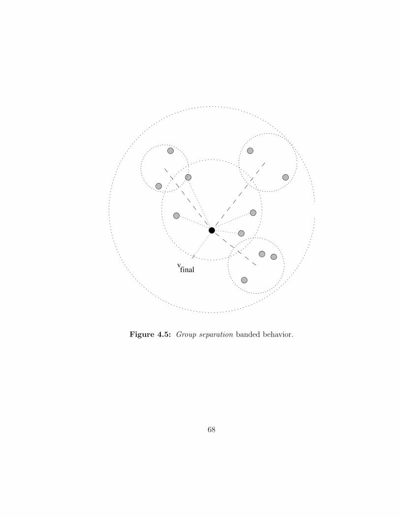
vfinal

Figure 4.5: Group separation banded behavior.

68

4.5.2.2 Cohesion

Like separation behavior, cohesion is modified to incorporate banding of dis-

tances where each band corresponds to a level in a grouping hierarchy. As before, in-

tragroup behavior is stronger than intergroup. Each band is appropriately weighted

during model calibration using the αb scale factor below. Each group’s center of

mass is calculated and scaled.

C =m∑

b=1

αb

nb

nb∑

i=0

pi,b (4.7)

where b is the band or group hierarchy and pi,b is the position of group member i,

which is an individual or another group, in band b. Finally, the weighted multi-

level center of mass C is subtracted from the agent of interest’s position P to yield

steering vector s,

s = P − C

Rather than the top-down view diagrammed in Figure 4.5 for separation, it can

be helpful to consider the tree structure of a group hierarchy. This is shown in

Figure 4.6. By coincidence, the nodes higher in the tree are separated by a greater

distance than those at lower levels, just how in reality the most local groups are the

most tightly packed. While the spacing in the figure is simply the by-product of how

it was drawn, it is a useful memory aid when considering separation and cohesion

within and among groups.

4.5.2.3 Agent Properties

Importantly, the group structure can be made still more complex by allowing

an individual group member to be any of a potentially large set of agents. More

concretely, it means we can have families made up not of identically acting agents

as nearly always the case in CAs, but made up of appropriately defined adults and

children. This is mentioned here to keep goals in context in forthcoming discussions,

and is described in depth in the next chapter in Section 5.3, Formal Language.

69

Groups ofgroups

Looser Spacing

Groups

IndividualPedestrians

Closer Spacing

Figure 4.6: Group tree structure.

For now, we continue exploring navigational techniques and move up a level from

segment traversal to route building.

4.6 Route Building

Segment traversal deals with moving from one point to another when there is

nothing obstructing the path. It deals only with pedestrian behavior while moving

freely. As soon as an obstruction is sensed between a pedestrian and his or her

destination, a route must be created by breaking the original segment into two or

more new ones. Pedestrian software agents, however, share with real pedestrians

limited awareness of their environment. They do not have built-in maps, or aware-

ness of what obstacles or walls lie beyond what they see at some moment. They

must choose courses based on what they perceive and what they might have already

learned from the environment.

70

4.6.1 Solids

The most basic avoidance scheme has been mentioned only passing. It is

solid body modeling that prevents one pedestrian from moving through another or

through walls and other obstacles. When all else fails in more elaborate collision

avoidance schemes and especially in highly congested areas, this is the fail safe that

always works! Two objects are not allowed to occupy the same space.

4.6.2 Obstacles

After solid body modeling, next in complexity is modeling smaller obstacles

that can be avoided by walking around them. A fountain in a shopping mall or

bed of flowers in a park are good examples. Recall, however, that there is more

to the goal than avoiding an obstacle. Group members continue to strive to re-

tain group structure, avoid other people, avoid interspersing with other groups, yet

make progress towards the destination. Obstacle avoidance does not preempt other

behaviors except when a collision is imminent.

Figure 4.7 illustrates the sequence of events used to navigate around obstacles.

At any point in time, a pedestrian always has a vector pointing from himself to his

destination, marked as X in the picture. Next, he creates a rectangle that is his

body width and a software adjustable length, usually ten times body width. An

affine transformation matrix is used to align the rectangle with the agent’s forward

direction. A quick intersection of the rectangle is then made against nearby obstacles

and the closest point of intersection, if any, is retained. This is the dot drawn in the

upper right frame of Figure 4.7. If no point of intersection exists, then there is no

need for obstacle avoidance.

When a point of intersection does exist, the obstacle is avoided by first cre-

ating a vector from the center of the obstacle pointing at the agent. If the agent is

71

dC

P

r = <x, y>

Figure 4.7: Obstacle avoidance

72

at point P and the obstacle center is at C, a repulsion vector r is

r = P − C =< x, y > (4.8)

A distance d is then calculated so that it is a few body widths beyond the edge of

the object. An arc can be struck as shown in the lower left frame of the figure so

that the center is at the object center and has radius d and that a line can be drawn.

We know from Pythagoras that if |r| > d there is a point on the arc such that a

right triangle can be created. The angle θ on the diagram is then

θ = arcsin

(

d

|r|

)

(4.9)

On the other hand, if the agent is within distance d of the object then the agent

simply takes an arbitrary orthogonal to r, say, < y,−x >. In words, this would be

the situation when an agent is so close to the object that he makes an immediate

right angle turn. That will only happen in this model if other factors have contin-

ually prevented an agent from deflecting his course, e.g., congestion or unfortunate

collision avoidance choices that mirror those of an oncoming pedestrian; the sort of

thing occasionally experienced when rounding an aisle while shopping.

Finally, the agent adjusts course to avoid the obstacle. Notice that no new

way point is used as an intermediate destination. At the next calculation, the same

steps are run through and course will be adjusted again. Eventually, the agent moves

beyond the obstacle, a collision avoidance check returns no point of intersection, and

it again resumes course towards the destination.

4.6.3 Walls

A pedestrian environment can be fully simulated only if the ability exists

to model walls. Walls are a part of almost all structures designed for human use.

While walls and small obstacles described above are similar in that they require a

person to navigate around them, there are important differences when creating a

mathematical model.

73

Avoiding obstacles requires short term planning by deciding how to make a

course change, but there is no change in destination and no need to remember past

efforts. It is a purely sense-react mechanism. Walls, however—even a single wall—

create a maze, to use the term loosely. That is, a wall presents a decision to the

person who walks towards it. The pedestrian must reach his or her destination by

walking to one end of the wall or the other, and sometimes the choice is wrong. In

order to correct mistaken choices, the software agent simulating a person must have

memory. In addition, it is mathematically slightly more involved to walk around a

long wall than an object whose edges span a relatively small portion of the field of

view.

In the model, an agent’s local neighborhood is scanned to see if any walls

are in the way. This is done the same way as described in obstacle avoidance by

intersecting a forward pointing rectangle with nearby walls. If a wall is modeled

with a line segment with end points A and B, we make a parallel unit vector w with

arbitrary direction:

w =B − A

|B − A|(4.10)

To move beyond the wall at point A with a standoff distance d, the agent would

head to the point P defined by

P = −dw + A (4.11)

Similarly, the stand off Q beyond the wall at point B is

Q = dw + B (4.12)

It is possible, however, that either A or B are interior corners and that the

corresponding standoff is blocked by the adjacent wall creating the corner. There-

fore, each stand off point is only considered if it is directly reachable by the agent.

74

4.6.3.1 Decisions

Now the agent knows which wall is in the way and must decide where to

go. Rather than consider only the blocking wall, it makes a list of all standoffs in

its neighborhood that can be reached without obstruction. Consider the standoffs

marked with letters in Figure 4.8. All are potential way points on the destination,

the open doorway at the upper right. Two things make a potential way point

appealing: 1) nearness, and 2) most nearly on-course. But before moving towards

one of these, the agent must make a decision and must have a way to remember it

and past decisions.

Past decisions are remembered by creating a decision tree. It’s current po-

sition P is used as the root and the root’s children are ranked, left to right in the

diagram, by nearness (we ignore consideration of remaining on-course here). A node

is shaded to indicate that it has been visited. In this tree, way point A is now used

as the next destination. At A, the figure shows that the agent can directly reach,

in order of nearness, way points B, C, P , and E. But P has been visited and is

anchored in place within the dynamically modified tree. That is, if a way point has

not been visited and is visible from the new current position, it is moved in the

tree to be a child of the current position. Once visited, though, it cannot again be

used except for backtracking which is described shortly. The new tree is shown in

the upper right frame of the figure. Subsequently, the agent moves to the highest

ranked unvisited child, B, and reorders the tree. Then to C where no reorganization

is needed, and finally to D when the tree can be destroyed because the destination

is unobstructed.

Note, however, that such a rigidly deterministic algorithm would result in

identical movement of all pedestrians; decidedly unrealistic. To add variability, or

another level of realism, we first consider the total distance that could be traveled

75

EAA

E

A

B

C E

A

B

C

D

A

B

C

D

E

E

P

A

B C

D

E

P

A

B C

D

1.P

B DC

2.P

D

B C

3. 4. 5.P

D

P

E

P

Figure 4.8: Decision tree building

76

to all these way points. That is,

r =5∑

i=1

|P −Qi| (4.13)

where Qi represents each of the five points A, B, C, D, and E. Then, distance from

P to each is normalized to range [0, 1] such that the closer the point is, the larger

its normalized value. For example, to point Qi, the normalized distance is simply

di =|P −Qi|

r(4.14)

Now we can draw a mathematical analogy from electrical engineering network anal-

ysis where we know the reciprocal of impedance is admittance. If the normalized

distances are thought of as electrical admittances, the largest admittance is the eas-

iest path for the bulk of the electrons, or, here, the greatest number of pedestrians.

Earlier we mentioned, however, that way point attractiveness is also based

on how close it is to the current course direction. So before making any way point

choice, the points are ranked again but based on needed course adjustment. From

the vector dot product definition we know that the angle between two vectors, A

and B is

θ = arccos

(

A ·B

|A||B|

)

(4.15)

So the way point preference can be ranked from smallest to largest θi for each

potential way point Qi. If, for instance, staying on course is most attractive and an

about face happens only 10% of the time, each way point would be ranked in the

range [0, 1] by

ci = 1−0.9

πθi (4.16)

for θ measured in radians.

The two weightings can be combined by weighting each based on model

calibration. A good value for willingness to explore seems to be:

wi = 0.7 di + 0.3 ci (4.17)

77

where wi is still in range [0, 1].

If a weight is, say, 0.4, it means 40% of pedestrians are likely to choose this

as its next way point. So the weights are now used as probabilities to make the final

ranking. Based on the probabilities, the children nodes are ranked based on a series

uniformly distributed random draws. For instance, if the sequence of wi above was

calculated as 0.4, 0.3, 0.2, 0.08, and 0.02, 40% of the time w1 is ranked first, 30% w2,

and so on. After the first ranking is chosen and that weight removed from the list,

the remaining weights are re-normalized and the ranking proceeds as described.

4.6.3.2 Backtracking

The example of Figure 4.8 showed a pedestrian fortunate enough to choose a

sequence of way points that brought it unerringly to its destination. As we learned

in the probabilistic ranking of the last section, it is certain that some pedestrians

will eventually choose way point E and walk there in hopes of reaching the hidden

destination as shown in Figure 4.9.

This unlucky agent moves to point E and now can see a corner at X and

modifies the decision tree as shown at (2) in the figure because from E it can only

see the unvisited way points X, B, and A. It visits X, adds Y to the tree, visits

Y , and then discovers no more way points can be added to the decision tree. It

has reached a dead end at (3) in the figure. The agent’s only recourse is to now

backtrack, working its way up the decision tree until reaching a previously visited

node that has at least one still unvisited child. In this example, the agent retraces

its steps to way point X which has no unvisited children. As a result it continues to

backtrack to already visited way point E and sees that E has a child, B, unvisited,

and the agent proceeds to B. Now the agent is on course to its destination via C

and D as in the last example.

A simplifying assumption of this research is that pedestrian areas are not

designed in a maze-like way, and in fact are designed to be easily traversable. While

78

D

P

3.

Y

X

E

X

A

B

B

P

B

P

X

Y

B A

DCE

4. P

E

X

Y C D A

2.

C D

A

P1.

BE C D A

E

P

A

B C

D

E

C

Figure 4.9: Decision tree backtracking

79

this decision tree method allows an agent in this model to remember everywhere

it has been, not especially realistic, and hence can eventually solve any maze, it is

important to note that the algorithms are not optimized for doing so. Part of making

an area easy to traverse is making information available to pedestrians to help them

make correct route choices. Incorrect choices not only frustrate pedestrians but

keep them in an area longer, increasing congestion or its likelihood of developing.

To simulate a real pedestrian area, then, the simulated pedestrians must be able

to learn. Like maze solving, a simplifying assumption here is that learning can be

simulated in a way that is simple but offers enough mimicry of real people that

predictions made by the model are reliable.

4.7 Learning

Simplified learning, or mimicry of learning, for pedestrians requires that an

agent

• has one or more destinations,

• be aware of whether or not it knows where the destinations are,

• the ability to search for a source of information,

• a way to transfer knowledge from an information source to itself, and

• a way to share knowledge with others.

Like all engineering tools, these requirements should be implemented in a

way that provides just enough power to do the job the tool was designed for. In

this case, the important aspect of learning in a real pedestrian environment is that

pedestrians must congregate at an information source and that it takes some time

for the transfer of information to happen. A small “You Are Here” sign in a complex

area will have people closely crowded around studying it for some length of time,

80

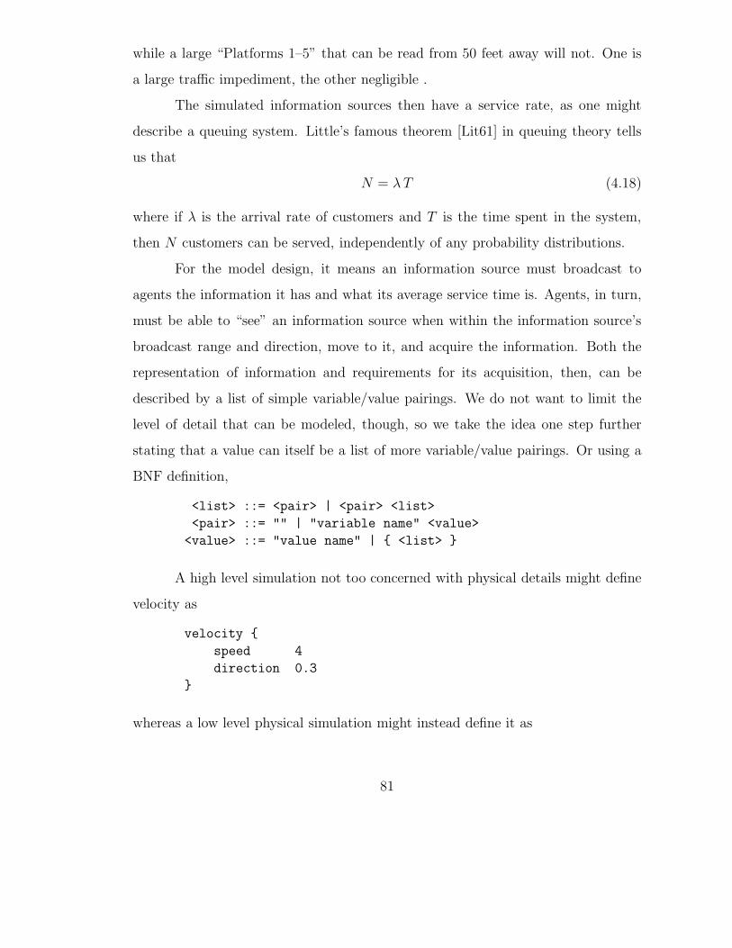
while a large “Platforms 1–5” that can be read from 50 feet away will not. One is

a large traffic impediment, the other negligible .

The simulated information sources then have a service rate, as one might

describe a queuing system. Little’s famous theorem [Lit61] in queuing theory tells

us that

N = λ T (4.18)

where if λ is the arrival rate of customers and T is the time spent in the system,

then N customers can be served, independently of any probability distributions.

For the model design, it means an information source must broadcast to

agents the information it has and what its average service time is. Agents, in turn,

must be able to “see” an information source when within the information source’s

broadcast range and direction, move to it, and acquire the information. Both the

representation of information and requirements for its acquisition, then, can be

described by a list of simple variable/value pairings. We do not want to limit the

level of detail that can be modeled, though, so we take the idea one step further

stating that a value can itself be a list of more variable/value pairings. Or using a

BNF definition,

<list> ::= <pair> | <pair> <list>

<pair> ::= "" | "variable name" <value>

<value> ::= "value name" | { <list> }

A high level simulation not too concerned with physical details might define

velocity as

velocity {

speed 4

direction 0.3

}

whereas a low level physical simulation might instead define it as

81

velocity {

speed {

magnitude 4

units m/s

}

direction {

magnitude 0.3

units radians

}

platformCapabilities {

maxSpeed 20

maxAngularVelocity 0.1

maxAccelaration 4

}

}

and so on.

Using variable/value pairs one can define service times, service rate distribu-

tions, broadcast range, etc., in addition to information of the simulated environment

itself, i.e., the data that agents exchange for their own decision making. An agent

is interested in finding an answer to its questions regarding where things are in its

world, whereas the workings of a simulator are interested in descriptions of agents

themselves, of sources and sinks that create and destroy agents, and of things like

obstacles and walls making up the environment itself. The flexibility to describe

multiple levels of objects related to the simulation is powerful by allowing modelers

to describe properties of agents and environment rather than having them built into

the model. Similarly, the same variable/value pairings can be used to represent the

state of the simulator at any instant in time, making it possible to pause and restart

simulations, possibly making modifications between.

At this point, agents have the ability to traverse segments while using modi-

fied, inter-group aware steering behavior; can avoid obstacles and other people; and

can locate information sources and learn destination locations from them. Through

the use of decision trees, they can also remember where they have been, and thereby

82

chain together segments of unobstructed paths into a complete route. The next and

final level of pedestrian modeling is one requiring advanced planning in the case of

real humans, scheduling.

4.8 Schedules

A schedule is a sequential list of goals to be completed by a certain time.

In a formalized sense, deadlines can be hard, soft, or non-existent [Mar98], where

hard means deadlines must be met, soft means some fraction must be met, and non-

existent means of course that there is no deadline for a scheduled goal. Deadlines in

a pedestrian system can usually be considered non-existent except in cases of depots

and other transportation related places where interchange schedules are strict, or

hard. Even though each goal has a deadline, with some notable exceptions, it can

be assumed that pedestrians have started their trips with time to spare.

However, by using the simple method of learning just described, it is possible

to allow simulated pedestrians to modify schedules. Even if there is a hard deadline

to catch a train at a certain time, it could be that an information source broadcasts

that it is a coffee shop, is open for business, average service time, and at that

8 am will be found attractive by 2% of passing commuters. Two percent of those

commuters whose schedules allow, based on the coffee shop’s service time estimate,

will then insert a new schedule entry with a soft deadline.

The two percent number in that example would have been chosen as the

result of real-life studies of a particular area. The rate of creation of agents and

their destruction, i.e., leaving the area encompassed by the simulation, as well as

placement of those sources and sinks, are also determined by real-life studies. The

outcome is that while scheduling is a difficult behavior to predict because it depends

on very human goals, not to mention whims, modeling scheduling at this level is

actually not terribly difficult. It amounts to studying an area and then placing

sources, sinks, attractors, and repellers in appropriate places. The studied attraction

83

E

D

P

Dest

Dest0

1Dest

nDest

Intermediate

Way Point

0

A

B C

Decision TreeNavigationSchedule

0

Figure 4.10: Schedule and decision tree feeding navigation stack

and repulsion properties results in expected population behavior so long as agent

behavioral attributes have been calibrated against people in the area of interest.

The best predictions will be the result of the best calibration data.

Back to schedules: If destinations either have no deadlines or deadlines far in

the future, the agent can rearrange the schedule to visit the nearest destinations for

which it has enough time. Similarly, if experienced service time turns out to be far

greater than the average, the schedule can again be rearranged so that deadlines can

be met. A schedule can then be thought of as a stack where the topmost entry is

popped off and added to the agent’s stack of planned destinations. This is illustrated

in Figure 4.10 where the schedule stack feeds the navigation stack. The navigation

stack in the picture would have come about as follows. When a destination was

pushed onto the stack the agent discovers no clear path exists from its position to the

new destination, so a decision tree is constructed. During the course of navigation

with the decision tree the currently targeted way point is added to the stack. The

way point when reached might be replaced by another from the decision tree until a

route to the destination is discovered. But while moving towards that way point the

agent in this example encounters an obstacle and repeatedly adds and then reaches

84

intermediate way points until it has moved around the obstacle. General steering

behavior is simple enough that it has no interaction with the navigation stack.

Therefore, during navigation there are several types of destinations. In addi-

tion to the final destination of the current route, there are intermediate destinations

used to avoid obstacles, as well as destinations from the decision tree. The final

destinations complete a route, but a schedule is made up of multiple routes. So only

after a route’s final destination is reached is the schedule used to feed another des-

tination to the navigation stack. Higher level decision making determines whether

or not a schedule may be modified by adding, reordering, or even deleting schedule

entries.

4.9 Summary

The pedestrian movement described in this chapter summarizes four levels

of movement. From simplest to most complex they are:

1. Segment traversal. This level uses steering behaviors drawn from Reynolds’

work and modified to support inter-group behaviors. By definition a segment

offers an open path to a destination.

2. Route traversal. When one or more obstacles block progress towards a

destination, a segment is broken up into additional segments. A route is

created by chaining together multiple segments. Group behavior and simple

learning can be involved in doing so.

3. Decision making. When a destination cannot be directly reached and there

is information teaching how to construct a route, agents’ memories are used

in the form of a decision tree.

4. Scheduling. At the highest level and the level that we as traveling humans

generally work at, schedules whose entries might have deadlines are made that

85

must be turned into routes and then segments using a combination of infor-

mation provided in the environment or trial and error coupled with memory.

86

Chapter 5

SIMULATOR DESIGN AND RESULTS

5.1 Introduction

Engineering is the application of science and mathematics in ways that are

useful to people. Having discussed the model itself, we now turn to implementing

it so that it can be used as a tool by civil engineers, urban planners, and architects.

Traditional engineering models capture system behavior from the top down. That

is, one or more partial differential equations are often used to capture the gross

properties of a system. As discussed, in this model properties are characterized only

at the lowest level and behavior emerges as the simulation unfolds. Rather than

use differential equations, algorithms are developed, and so it is worth taking a few

moments to compare algorithm and software development to the traditional, purely

mathematical approach.

In the field of computability theory, Davis and Weyuker [DW83] define a

primitive recursively closed class of functions as one where:

1. the initial functions belong to the class,

2. a function obtained from functions belonging to the class by either composition

or recursion also belongs to the class.

87

Instruction Interpretation

V ← V + 1 Increase by 1 the value of the variable V .

V ← V − 1If the value of V is 0, leave it unchanged; otherwisedecrease by 1 the value of V .

IF V 6= 0 GOTO LIf the value of V is nonzero, perform the instruc-tion with label L next; otherwise proceed to thenext instruction in the list.

Table 5.1: Minimal programming language

It turns out that initial functions can be very simple and will be

s(x) = x + 1, (5.1)

n(x) = 0, (5.2)

uni (x1, . . . , xn) = xi, 1 ≤ i ≤ n. (5.3)

Now consider a primitive programming language made up of three simple statements

(taken from [DW83]) and shown in Table 5.1.

With a small effort this simple programming language can be used to com-

pute the initial functions s, n, and uni , whose names, respectively, are successor, null,

and projection. Through a much greater effort, it can be shown that this simple

language can implement a Universal Turing Machine which in turn can be used to

compute any computable algorithm. But these algorithms are in fact compositions

and recursions of the initial functions given above. Using words to describe that,

algorithmic development is as mathematical at its core as partial differential equa-

tions, but the many layers of abstraction sometimes make it difficult to see. The

pedestrian model described uses physical modeling, clearly mathematical in nature,

88

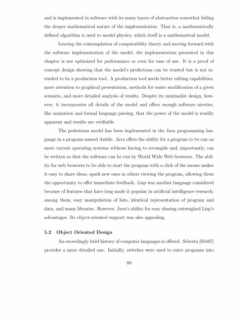
and is implemented in software with its many layers of abstraction somewhat hiding

the deeper mathematical nature of the implementation. That is, a mathematically

defined algorithm is used to model physics, which itself is a mathematical model.

Leaving the contemplation of computability theory and moving forward with

the software implementation of the model, the implementation presented in this

chapter is not optimized for performance or even for ease of use. It is a proof of

concept design showing that the model’s predictions can be trusted but is not in-

tended to be a production tool. A production tool needs better editing capabilities,

more attention to graphical presentation, methods for easier modification of a given

scenario, and more detailed analysis of results. Despite its minimalist design, how-

ever, it incorporates all details of the model and offers enough software niceties,

like animation and formal language parsing, that the power of the model is readily

apparent and results are verifiable.

The pedestrian model has been implemented in the Java programming lan-

guage in a program named Amble. Java offers the ability for a program to be run on

most current operating systems without having to recompile and, importantly, can

be written so that the software can be run by World Wide Web browsers. The abil-

ity for web browsers to be able to start the program with a click of the mouse makes

it easy to share ideas, spark new ones in others viewing the program, allowing them

the opportunity to offer immediate feedback. Lisp was another language considered

because of features that have long made it popular in artificial intelligence research;

among them, easy manipulation of lists, identical representation of program and

data, and many libraries. However, Java’s ability for easy sharing outweighed Lisp’s

advantages. Its object-oriented support was also appealing.

5.2 Object Oriented Design

An exceedingly brief history of computer languages is offered. Sebesta [Seb07]

provides a more detailed one. Initially, switches were used to enter programs into

89

Public Interface

Pu

bli

c In

terf

ace Private Processing

HiddenData

Pu

blic In

terface

Public Interface

Class definition X

Public Interface

Pu

bli

c In

terf

ace Private Processing

Hidden Data

Class X

Pu

blic In

terface

Public Interface

Class definition Y

Figure 5.1: Object and inheritance.

computers by binary on-off patterns but assembly language soon followed, allowing

the use of mnemonics in place of binary patterns. It also allowed more complex

control structures letting the programmer avoid repeating code through the use of

loops and subroutines. Higher level languages like the procedural Fortran, block

structured Algol, functional Lisp, and many others followed, each viewing problem

solving from a slightly different point of view. The latest addition to data abstrac-

tion is object oriented programming. The basic tenets in this paradigm are that

processing is encapsulated and data is hidden. Another feature, inheritance, allows

a new object to take on all attributes of another and then extend it still further.

Figure 5.1 diagrams an object on the left and shows an example on the right of

an object Y which has inherited the X. Objects communicate solely through their

public interfaces, and some of the interfaces can exist as the result of inheritance

and some unique to that class of object.

Java is an object oriented language which lends itself well to agent-based

simulations. When considering a pedestrian, it is natural to model one as an object,

a thing with its own processing powers and its own unique state. Processing powers

90

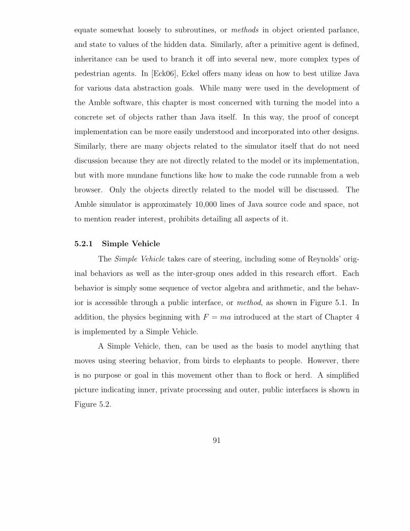
equate somewhat loosely to subroutines, or methods in object oriented parlance,

and state to values of the hidden data. Similarly, after a primitive agent is defined,

inheritance can be used to branch it off into several new, more complex types of

pedestrian agents. In [Eck06], Eckel offers many ideas on how to best utilize Java

for various data abstraction goals. While many were used in the development of

the Amble software, this chapter is most concerned with turning the model into a

concrete set of objects rather than Java itself. In this way, the proof of concept

implementation can be more easily understood and incorporated into other designs.

Similarly, there are many objects related to the simulator itself that do not need

discussion because they are not directly related to the model or its implementation,

but with more mundane functions like how to make the code runnable from a web

browser. Only the objects directly related to the model will be discussed. The

Amble simulator is approximately 10,000 lines of Java source code and space, not

to mention reader interest, prohibits detailing all aspects of it.

5.2.1 Simple Vehicle

The Simple Vehicle takes care of steering, including some of Reynolds’ orig-

inal behaviors as well as the inter-group ones added in this research effort. Each

behavior is simply some sequence of vector algebra and arithmetic, and the behav-

ior is accessible through a public interface, or method, as shown in Figure 5.1. In

addition, the physics beginning with F = ma introduced at the start of Chapter 4

is implemented by a Simple Vehicle.

A Simple Vehicle, then, can be used as the basis to model anything that

moves using steering behavior, from birds to elephants to people. However, there

is no purpose or goal in this movement other than to flock or herd. A simplified

picture indicating inner, private processing and outer, public interfaces is shown in

Figure 5.2.

91

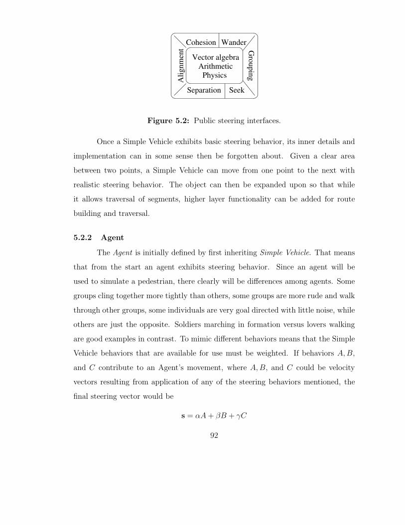
Ali

gn

men

t

Cohesion Wander

Gro

up

ing

SeekSeparation

Vector algebraArithmetic

Physics

Figure 5.2: Public steering interfaces.

Once a Simple Vehicle exhibits basic steering behavior, its inner details and

implementation can in some sense then be forgotten about. Given a clear area

between two points, a Simple Vehicle can move from one point to the next with

realistic steering behavior. The object can then be expanded upon so that while

it allows traversal of segments, higher layer functionality can be added for route

building and traversal.

5.2.2 Agent

The Agent is initially defined by first inheriting Simple Vehicle. That means

that from the start an agent exhibits steering behavior. Since an agent will be

used to simulate a pedestrian, there clearly will be differences among agents. Some

groups cling together more tightly than others, some groups are more rude and walk

through other groups, some individuals are very goal directed with little noise, while

others are just the opposite. Soldiers marching in formation versus lovers walking

are good examples in contrast. To mimic different behaviors means that the Simple

Vehicle behaviors that are available for use must be weighted. If behaviors A, B,

and C contribute to an Agent’s movement, where A, B, and C could be velocity

vectors resulting from application of any of the steering behaviors mentioned, the

final steering vector would be

s = αA + βB + γC

92

where α, β, and γ weight the behaviors. The wander behavior in the case of marching

soldiers would be close to zero, where seek in the case of emergency evacuation would

be the highest weighted vector with the exception, perhaps, of cohesion with a child

or other dependent group member.

Behavior gets more complicated with obstacle and wall avoidance, however,

because weighting is not straightforward. When viewed instantaneously, all weights

but avoidance drop to zero approaching an imminent collision. But the weights

drop gradually between the states of unobstructed travel and eventual collision. In

this in-between state, steering behaviors are still followed but weighted less and less

as the potential collision approaches. Agents in Amble deal with this by sensing

their immediate neighborhood, which is described as a radius of some length cen-

tered at their position. Anything outside the local neighborhood is not sensed and,

hence, does not affect steering and higher level behavior. Once something is sensed,

however, immediate collision avoidance commences. At first glance, it seems this

would destroy all behavior related to grouping. It is unlikely, however, that all group

members would sense a collision simultaneously since some will naturally be closer

or farther than others. The result is that the lagging members continue to behave

as before. Often, by the time the first member to have sensed a collision has avoided

it, the lagging members are just noticing. But at this point it is the lead members

that now follow grouping behavior. So inter- and intra-group behavior survives col-

lision avoidance mostly intact. At this point, an agent can move from one point to

the next even if there are obstructions in between. Importantly, though, it cannot

remember where it has been. Building on the previous object diagram, its abilities

are shown in Figure 5.3.

5.2.3 Navigation Stack, Decision Tree, and Schedule

The ability to avoid walls but having no memory of past attempts obviously

does not mimic human behavior. The decision tree developed in the last chapter

93

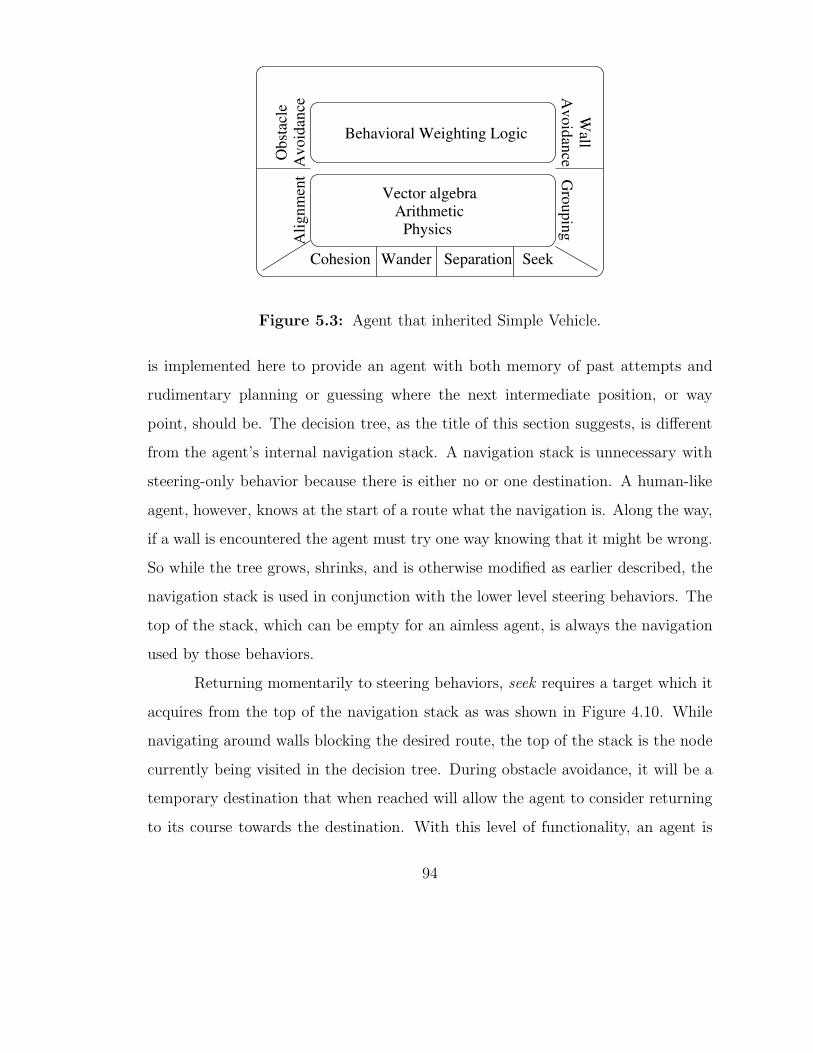
Ob

stac

leA

vo

idan

ce

Behavioral Weighting Logic

Av

oid

ance

Wall

Ali

gn

men

t

Vector algebraArithmetic

PhysicsG

rou

pin

gCohesion Wander Separation Seek

Figure 5.3: Agent that inherited Simple Vehicle.

is implemented here to provide an agent with both memory of past attempts and

rudimentary planning or guessing where the next intermediate position, or way

point, should be. The decision tree, as the title of this section suggests, is different

from the agent’s internal navigation stack. A navigation stack is unnecessary with

steering-only behavior because there is either no or one destination. A human-like

agent, however, knows at the start of a route what the navigation is. Along the way,

if a wall is encountered the agent must try one way knowing that it might be wrong.

So while the tree grows, shrinks, and is otherwise modified as earlier described, the

navigation stack is used in conjunction with the lower level steering behaviors. The

top of the stack, which can be empty for an aimless agent, is always the navigation

used by those behaviors.

Returning momentarily to steering behaviors, seek requires a target which it

acquires from the top of the navigation stack as was shown in Figure 4.10. While

navigating around walls blocking the desired route, the top of the stack is the node

currently being visited in the decision tree. During obstacle avoidance, it will be a

temporary destination that when reached will allow the agent to consider returning

to its course towards the destination. With this level of functionality, an agent is

94

now able to move from one point to another, while avoiding obstacles, avoiding walls

and remembering its path for possible backtracking. In all other cases, the top of

the destination stack is sequentially fed from the agent’s schedule.

The agent builds a schedule based on real world data acquired by studying

a real pedestrian area or based on hypotheses by experienced professionals. For

instance, if certain real restaurants in a given area of the city attract about 50

people per hour during lunch time, and that same general area has 5,000 people

move through during that period, then agents in the simulation will find a simulated

restaurant to attract them to it 1% of the time. Or, with a probability of 0.01 they

will add that destination to their schedule.

So again visiting Figure 4.10, it is natural in the software implementation to

use three objects to implement each of the the three entities there. Figure 5.4 shows

what the software agent looks like with the addition of the new agent capabilities

of memory, decision making, and trip completion. At last, an agent is working at

a high enough level that it creates its schedule and then only has to proceed. All

lower level processing happens in a hidden way, somewhat analogous to subconscious

reasoning.

5.2.4 Sources and Sinks

In real life people move from place to place, strangers appear and disappear

from our sight. In a simulated world, the agents must truly appear and disappear.

When they leave the scope of the simulated world they cease to exist. They similarly

pop into being during their simulated arrival as a result of exiting a train or a

store and suddenly appearing in the simulated world. In Amble, sources and sinks

perform those functions. As with most things, it is easier to destroy than create.

When an agent reaches its destination sink, it is permanently removed from the

simulated world. Sources are more involved because they must create different types

of agents and must do so in a realistic way. Whether Poisson, uniform, exponential,

95

Follow Schedule Make Schedule

Trip Scheduling

MemoryDestination

Stack

Ob

stac

leA

vo

idan

ce

Behavioral Weighting Logic

Wall

Av

oid

ance

Gro

up

ing

Vector algebraArithmetic

Physics

Ali

gn

men

t

Cohesion Wander Separation Seek

Figure 5.4: Complete agent.

96

or other distribution, the arrival process must be chosen to model to appropriately

characterize its real life complement. An additional complexity is that while the

environment is populated by people, the source also creates the social groupings

that are not visible. More detail is provided in the following section describing the

Amble formal language.

5.3 Formal Language

Like overlapping circles in a Venn diagram, several areas in the Amble imple-

mentation of the pedestrian model all coincide in one area, the need for descriptions:

1. Agent behavior must be described,

2. The environment must be described,

3. Simulation state must be described.

Agent behavior has the most obvious need for description because the only alterna-

tive would be to hard code agent behavior into the software. That clearly limits the

usefulness of the tool to only situations where the real pedestrians happen to act

similarly to the hard coded ones. Agents need a language with enough flexibility to

describe behaviors. In order for agents to learn, they must be able to observe their

environment, understand it in a simple way, and mimic learning from it. Therefore,

items in the environment need to have descriptions that agents can use. This is at

a different level of abstraction than describing agent behavior. Finally, the state

of the simulator at any point must be describable so that it can be started with

objects placed at specified locations, sources and sinks acting in particular ways,

and so on. State descriptions also allow the simulator to be paused or stopped

and resumed at a later time. Summarizing, descriptions are used by real people to

describe simulated pedestrian behavior, used by simulated pedestrians to interact

with their environment, and by the simulator to control the simulation.

97

One simple formal language which will accomplish all three tasks is pre-

sented below. It is based completely on the variable/value discussions of Section 4.7

regarding agent learning. While the language syntax is nothing more than the vari-

able/value enumerations, the simulator does expect certain keywords. The syntax

is straightforward. A variable name is a text string and an atomic value is also a

string. Values, however, may themselves be lists of more variable/value pairs, and

so are delimited by curly braces. Expanding on the BNF definition given in the last

chapter, the Amble description language follows the syntax,

<list> ::= <pair> | <pair> <list>

<pair> ::= "" | "variable name" <value>

<value> ::= "value name" | { <list> }

Of even greater importance to the modeler, though, are the keywords so that par-

ticular variable names can be tied to behavioral and other properties of Amble. A

scenario description contains three blocks:

static {

}

initial {

}

dynamic {

}

where the block names are fairly descriptive. The static block contains descriptions

mainly of agent behaviors, while the initial block describes the placement of

objects in the environment. Finally, the dynamic block stores the instantaneous

state of the simulation. It is only used in the case of pausing and saving a simulation,

or when later reloading it. Because the identical description syntax is used to

represent behavioral properties, information in the environment, and knowledge

in the agent, a paused simulation’s dynamic state can be saved including agent-

acquired knowledge, current schedule and so on.

98

5.3.1 The Static Block

The static block supports two descriptions: display size, in pixels, of the

environment so it can be mapped to the desired area on the screen; and agent types

and behaviors.

The environment description uses the keyword world along with width and

height variables.

world {

width 1000

height 1000

}

Description of agents is more involved and is included within the agents

block. It includes sub-blocks whose names are chosen by the modeler and whose

lists are made up of keywords. Examples follow.

agents {

adult {

// Adults are dark green.

color { r 99 g 167 b 97 }

size { radius 5 }

speed 15

vectorWeights {

seek 90

wander 80

separation 30

cohesion 100

}

}

child {

// Kids are light blue.

color { r 125 g 247 b 255 }

size { radius 4 }

speed 15

vectorWeights {

seek 90

99

wander 90

separation 40

cohesion 90

}

}

family {

cohesion 100

separation 20

members {

adult {

// Probability Quantity

0.2 1

0.8 2

}

child {

// Must be in increasing prob. order!

0.05 4

0.10 3

0.15 1

0.70 2

}

}

}

}

First, notice that comments begin with the “//” sequence. Next, we see that

three agent types are defined: adult, child, and family, where family is an agent

made up of other agents. The names adult, child, and family are user chosen

whereas all other variable names are keywords expected by Amble. Agent color is

defined by the variable color whose value is always a list containing six elements

which are the letters r, g, b, each immediately followed by an 8 bit decimal value,

that is, a number in the range from 0 to 255. Each of red, green and blue can have

intensities ranging from very dark (0) to very light (255). For instance, black is

attained when all three of RGB are zero, and white when all of RGB are 255. Agent

geometry, as shown in the example, is currently limited to a circle of user defined

100

radius, in units of pixels. It is straightforward to support other shapes, but the focus

of the research is on the behavioral aspects rather than the display. The value of

speed is an integer in units of pixels relative to the specified size of the environment

earlier in the static block.

The most important sub-block is vectorWeights where the modeler defines

the relative weights of each steering vector. Each integer weight can be any value.

This makes it easy to stretch or shrink a value during calibration without worrying

about having everything add up to some required value like 1 or 100.

Creating groups adds more complexity because groups don’t have the same

make up or even behavior as their constituent components. The example defines

the members of a family as some combination of adult and child. To consider the

example line by line, there is a 20% chance of a family having one adult and 80%

chance of having two. This example also imposes the constraint that every family

contains between one and four children, where 5% contain 4, 10% contain 3, 15%

contain 1, and 70% contain 2 children. Additionally, a family group has its own

steering vectors as described in detail last chapter. As before, the vector integer

values are relative to each other and the absence of a vector type implies a weight

of zero. Since group boundaries are generally not drawn, choosing a group color

has no effect on its display. (Examples in this dissertation do, in fact, show group

boundaries for ease of interpretation of the figures.)

The modeler, then, has the ability to describe agent size and color, speed,

and behavior as defined by steering vectors. Furthermore, groups are defined by

their probabilistic make up, and higher level steering vector weightings. This offers

great flexibility for the modeler in allowing him or her to model a wide variety of

situations. A scenario might include single commuters, groups of friends, groups of

families, and even higher level groups of groups. The last might be the case when a

group of families goes on a picnic together or when a group of couples go to a dance.

101

5.3.2 The Initial Block

This second of the major blocks in the Amble language deals with initial sce-

nario set up. It contains descriptions both of the visible simulated world and prop-

erties of some objects. The keywords recognized in this block are sinks, sources,

walls, and objects.

5.3.2.1 Walls

Walls are easily described as line segments whose endpoints are (x0, y0) and

(x1, y1).

walls {

left {

position { x0 10 y0 10 x1 10 y1 400 }

}

right {

position { x0 400 y0 10 x1 400 y1 400 }

}

rightii {

position { x0 325 y0 10 x1 325 y1 325 }

}

rightiii {

position { x0 260 y0 75 x1 260 y1 325 }

}

top {

position { x0 10 y0 10 x1 400 y1 10 }

}

topii {

position { x0 75 y0 75 x1 260 y1 75 }

}

bottom {

position { x0 10 y0 400 x1 400 y1 400 }

}

bottomii {

position { x0 260 y0 325 x1 325 y1 325 }

}

}

102

The wall names such as rightii are user given. The integer coordinates are relative

to the world, i.e., size given in the static block and can be thought of as pixels,

even though the mapping from model to screen pixels might not actually be one to

one.

5.3.2.2 Obstacles

Descriptions of obstacles in the environment are more involved. The simplest

obstacle is what one would expect. It has some size and position and pedestrians

must avoid bumping into it. In contrast, a “You Are Here” sign not only must not

be bumped into, but also contains useful information for pedestrians and has some

probability of attraction. Some service time is also associated with either the act

of learning or what might be thought of as browsing. In the latter case, consider

an exhibition hall or market place where each table or display holds the interest of

passersby for some length of time. The simplest obstacle which has no interest to

pedestrians other than its avoidance might be described this way:

A {

center { x 200 y 150 }

radius 30

}

where the object is bounded by the described circle. Long, skinny objects can be

bounded by a sequence of overlapping circles. The name A is user chosen in the same

way that agent names were. Imagine now that the same obstacle is an interesting

poster exhibition at a conference. It could be described as

poster {

center { x 200 y 150 }

radius 30

attraction { professor 0.2

student 0.5

companyMan 0.1 }

serviceTime { professor 111

student 250

103

companyMan 300 }

distribution exponential

}

meaning that 20% of professors, 50% of students, and only 10% of company men,

all agents that would have been described in the static block, will find this poster

interesting to walk towards. Upon arrival, the average service time, i.e., time spent

looking, reading, and talking, at the poster would be, in units of simulated seconds,

111 for professors, 250 seconds for students who will take longer to understand, and

300 seconds for the pretend company personnel who have been away from school a

long time.

The most complex object is the type that can impart information to agents.

In a pedestrian environment the information of importance is that relating to other

parts of the environment. This might be a map

infoMap {

info {

place {

A 0

B 0

C 0

D 0

E 0

F 0

}

}

center { x 500 y 150 }

radius 30

attraction { local 0.1

tourist 0.6 }

serviceTime { local 30

tourist 180

distribution exponential

}

that offers information on obstacles A, B, C, D, E, and F. The zeros by each

info/place name are unused dummy values to maintain the variable/value syntax.

104

Rather than duplicate information here, the simulator locates the referenced object

and provides the agent with the information. Information could be, for instance,

location or estimated service time for scheduling decisions. In this example, the

10% of local residents who read the sign would only require 30 seconds of reference,

while the 60% of tourists need 3 minutes on average. The information is then moved

“inside” the agent and becomes part of its knowledge for decision making.

5.3.2.3 Sinks and Sources

Sources are objects that create pedestrians and sinks destroy them. They

represent the arrivals and departures of pedestrians in a given area. A source peri-

odically creating 40 agents at a corner might represent that number of people getting

off a bus at scheduled times. Similarly, if a shopping mall design is being studied,

sinks would be used to remove departing pedestrians as they reach simulated exits.

Sinks are clearly the easier of the two to implement. They are described by

their locations and radius as well as how attractive, probabilistically, they are to

passing agents. This snippet of an Amble description illustrates the details.

sinks {

lowerRight {

position { x 990 y 520 }

radius 10

probabilities {

// Everyone uses this sink with probability 1.

adult 0.5

child 0.5

}

}

upperRight {

position { x 990 y 30 }

radius 10

probabilities {

// Everyone uses this sink with probability 1.

adult 0.5

child 0.5

105

}

}

}

The modeler has created two sinks and named them lowerRight and upperRight.

Position and radius are, as usual, in units relative to those given in the static

block. The probabilities list is similar in nature to that used in the previously

described obstacles. For each adult and child, in this example, it will use either sink

with a probability of 0.5.

Sources require more description by the modeler because of their more com-

plex behavior. Here is an example:

sources {

upperLeft {

position { x 30 y 30 }

// Set internal queue size.

qlen 60

// Uniform probability of entity creation/time step.

process uniform

p 0.0035

// What to create.

agents {

// Create commuters and families.

family 0.2

commuter 0.8

}

}

}

In the case of sources, position is important but there is no need for size since the

created agents are simply placed at the specified position. A bus, doorway, stairwell,

and other suppliers of people all have a finite (instantaneous) capacity and can be

modeled using a queue. Queue arrival patterns can be specified and service times are

zero with an important constraint. Immediately upon creation, agents are placed

in the finite length queue. If the source position is unoccupied, the first agent in

106

the queue is immediately placed there. At each time increment in the simulation,

every source queue is serviced as congestion allows. The qlen keyword is used to

specify the length of the queue. When the congestion level is high it is possible for

the queue to fill, at which time the sources cease creating new agents.

Agents are most commonly created using a uniform process but others can

be specified, like Poisson and exponential. It is a simple exercise to add new arrival

processes to Amble when necessary. For the uniform case an associated probability

p, the probability that an agent will be created this time step, is defined. The

Poisson process requires an intensity value to specify its arrival intensity. There

is also a oneShot process, mainly used for model testing, instructing a source to

create exactly one agent.

Finally, the agents section is a list of probabilities that add up to one. When

a new agent is to be created this probability list is used to randomly determine which

will be created. In the example above, when an agent will be created, 20% of the

time it will be a family and 80% a commuter. Notice that a family agent is composed

of several members, and that it is not necessary to tell the source the specifics of the

family composition. The source creates agents in a recursive manner. Using pseudo-

code and ignoring the details of assigning individual behavior which is captured in

attributes below:

Enqueue-Agent(type, parent)

1 agent ← Create-Agent(type)

2 attributes ← Create-Individual-Attributes()

3 if parent 6= null

4 parent.Add-Member(agent)

5 if type = group

6 Make-Group(attributes, agent)

7 else

107

8 Enqueue(agent)

Make-Group(attributes, agent)

1 n ← Get-Num-Members(attributes)

2 for i ← 1 to n do

3 type ← Get-Member-Type(attributes)

4 Enqueue-Agent(type, agent)

An important point that might not be readily apparent in the pseudo code

is that not all agents are added to the queue; only those that have no members.

Not having members means an agent is atomic. For instance, a family has members

but a person does not. So only “bodies” are queued. This is because the queue

offers people to the environment. Any relationships are important only to the group

members, not to the queue or environment.

5.3.3 The Dynamic Block

This is the easiest of the three major Amble blocks to describe. The dy-

namic block is used only when a running simulation is paused. Every attribute for

each agent’s current state is written out in the variable/value syntax of the Amble

language. Information for every wall, obstacle, source, sink, and the environment

already exists in the Static and Initial blocks and doesn’t need to be repeated

in Dynamic. When Amble starts up next and is given as input a file generated by

pausing the simulation, it first reads in and appropriately acts on the information

in the Static and Initial blocks, and then reads in the dynamic agent data. In a

sense, the reading in of dynamically created agent data can be thought of as a super

source; a source that not only can create new agents, but can also create agents in

mid-travel and with some level of environmental knowledge.

108

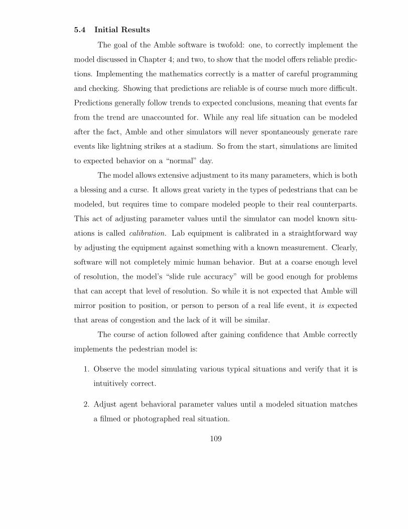
5.4 Initial Results

The goal of the Amble software is twofold: one, to correctly implement the

model discussed in Chapter 4; and two, to show that the model offers reliable predic-

tions. Implementing the mathematics correctly is a matter of careful programming

and checking. Showing that predictions are reliable is of course much more difficult.

Predictions generally follow trends to expected conclusions, meaning that events far

from the trend are unaccounted for. While any real life situation can be modeled

after the fact, Amble and other simulators will never spontaneously generate rare

events like lightning strikes at a stadium. So from the start, simulations are limited

to expected behavior on a “normal” day.

The model allows extensive adjustment to its many parameters, which is both

a blessing and a curse. It allows great variety in the types of pedestrians that can be

modeled, but requires time to compare modeled people to their real counterparts.

This act of adjusting parameter values until the simulator can model known situ-

ations is called calibration. Lab equipment is calibrated in a straightforward way

by adjusting the equipment against something with a known measurement. Clearly,

software will not completely mimic human behavior. But at a coarse enough level

of resolution, the model’s “slide rule accuracy” will be good enough for problems

that can accept that level of resolution. So while it is not expected that Amble will

mirror position to position, or person to person of a real life event, it is expected

that areas of congestion and the lack of it will be similar.

The course of action followed after gaining confidence that Amble correctly

implements the pedestrian model is:

1. Observe the model simulating various typical situations and verify that it is

intuitively correct.

2. Adjust agent behavioral parameter values until a modeled situation matches

a filmed or photographed real situation.

109

Figure 5.5: Seek simulation.

3. Offer predictions of new situations.

The examples in the remainder of this section fall into category (1) above.

While the simulator presents animated pedestrians, which make intuitive checks

easier, still shots by necessity are presented here.

5.4.1 Simple Steering Behavior

The first few images build up several of Craig’s steering behaviors to form

the basis of the more complex behaviors that are subsequently layered on these.

Figure 5.5 shows the two simplest properties of pedestrians: solid body modeling

and destination seeking. There is no ability to move around a slower pedestrian, or

more correctly, no awareness that it can be done. The result is an impatient looking

line of people, some bumping against the next.

Figure 5.6 adds just a little more realism by making agents conscious of

separation. They still don’t know how to pass one another, but they no longer

bump into each other.

When some correlated noise is added to the previous behaviors, the first

signs of realistic travel appear. In this case, as shown in Figure 5.7, pedestrians

110

Figure 5.6: Seek and Separation simulation.

can now pass one another though they still seek their destinations and try to honor

a separation distance. The random noise can make separation impossible every so

often. For instance, if one pedestrian happens to move to the right just as a nearby

neighbor traveling in parallel happens to move to the left, only solid body modeling

solves the problem with a collision.

With seek, separation, and wander, only awareness of walls must be added to

create useful simulations. This stage, incidentally, is where the majority of current

pedestrian models stop. While walls are to be avoided, doorways are to be targeted

during an evacuation. Figure 5.8 shows how simple behaviors result in a quite

realistic looking situation. It can also model the start of a grade school day, where

rather than evacuation there is entrance-way congestion.

Figure 5.9 is a simulation of family groups walking. Notice how the smaller

circles, the simulated children, tend to have greater intragroup cohesion than the

adults. Additionally, there is clear separation both within and between groups. They

display the basic steering properties at, in this case, two levels. Group memberships

are unmistakable, yet all pedestrians move towards their destinations.

111

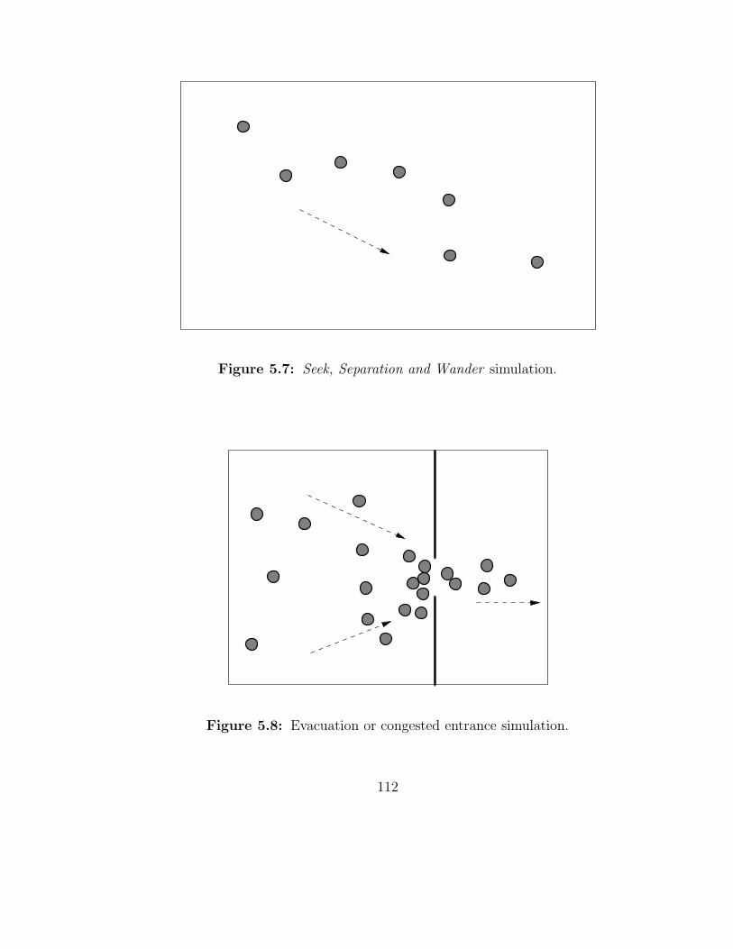
Figure 5.7: Seek, Separation and Wander simulation.

Figure 5.8: Evacuation or congested entrance simulation.

112

Figure 5.9: Family group simulation.

It is more difficult on paper to demonstrate weaving among groups. Fig-

ure 5.10 is a snapshot of families avoiding each other while traveling towards desti-

nations that had put them on a collision course. In this case, they were able to avoid

interspersing with each others’ groups. All group members made course adjustments

so that a collision would be avoided, group structure was maintained, and group in-

terspersal was avoided. In higher congestion, however, it turns out that intergroup

separation and intragroup cohesion can be balanced so that groups do indeed in-

tersperse. This sort of behavior is what one would intuitively expect in a crowded

situation. Only pedestrians with small children or other extreme dependents would

never allow strangers to come between them.

The more complicated the simulated behavior the more difficult it is to cap-

ture in still pictures. But Figure 5.11 illustrates a crowd of people who have sched-

ules which are indicated by the floating letters by the groups. The order of the

letters indicates the order of places that each group will visit. Each destination has

an average service time, or visit time, by the pedestrians. To make matters more

difficult, though, the pedestrians don’t always know where a destination is located.

113

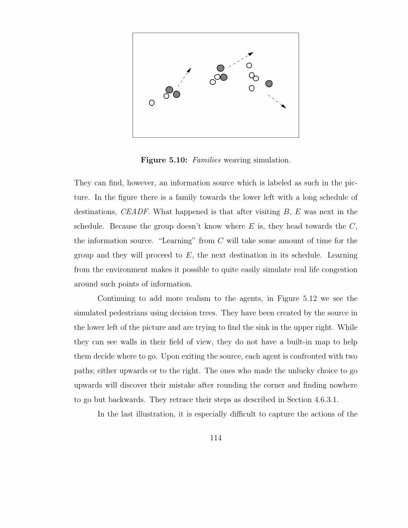
Figure 5.10: Families weaving simulation.

They can find, however, an information source which is labeled as such in the pic-

ture. In the figure there is a family towards the lower left with a long schedule of

destinations, CEADF. What happened is that after visiting B, E was next in the

schedule. Because the group doesn’t know where E is, they head towards the C,

the information source. “Learning” from C will take some amount of time for the

group and they will proceed to E, the next destination in its schedule. Learning

from the environment makes it possible to quite easily simulate real life congestion

around such points of information.

Continuing to add more realism to the agents, in Figure 5.12 we see the

simulated pedestrians using decision trees. They have been created by the source in

the lower left of the picture and are trying to find the sink in the upper right. While

they can see walls in their field of view, they do not have a built-in map to help

them decide where to go. Upon exiting the source, each agent is confronted with two

paths; either upwards or to the right. The ones who made the unlucky choice to go

upwards will discover their mistake after rounding the corner and finding nowhere

to go but backwards. They retrace their steps as described in Section 4.6.3.1.

In the last illustration, it is especially difficult to capture the actions of the

114

A C

B D

B F

C E A D F

C A E

C B D

F B A

D F

INFO

D F

D

F B A

Figure 5.11: Learning simulation.

115

Figure 5.12: Decision tree simulation.

116

Figure 5.13: Maze simulation.

lone pedestrian. A one shot source is located in the lower left of Figure 5.13 and the

pedestrian’s goal is the sink at the upper right. As mentioned previously, Amble

pedestrians are not at all optimized to be maze solvers. But by knowing how to avoid

walls and by being able to build decision trees, a pedestrian is able to thread his way

through the maze. The figure shows the happy pedestrian having just completed

his quest.

5.5 Final Results

The examples of the last section seem intuitively correct, but to rely on Amble

predictions, simulations must closely match recorded events. This section is devoted

to comparisons made between photographed areas and simulations.

117

5.5.1 Calibration

The first step is to calibrate the model. The weighting of steering vectors and

probabilities regarding decision making can be adjusted. Calibration of the model

means that distances between individuals and groups, average speeds, and collision

avoidance mechanisms must, after scaling time and distances appropriately, match.

Fruin’s landmark study [Fru71], is the standard for current design efforts and is cited

in many guidelines. Still [Sti00] points out that Fruin’s work is based on studies

conducted on city streets, and that crowd dynamics are different, for instance, in

stadiums or in evacuations. Because the focus of this research is modeling of typical

rather than extreme situations, calibration using Fruin’s data is appropriate.

Regarding pedestrian group behavior, Tarawneh [Tar01] studied the behav-

iors of how groups walked together. His results verify what one might intuitively

assume; that males walk faster than females, the young walk faster than the elderly,

and groups walk more slowly than individuals. Because the model presented in this

thesis combines weighted and sometimes competing vectors, it is not surprising that

groups also walk more slowly than individuals. Individuals in the model have no

concern for retaining group structure, and hence many of the competing velocity

vectors do not exist. In groups, obviously this is not the case. The greater number

of vectors contributing to the overall velocity will on occasion cancel out portions

of other contributing vectors. It is interesting to consider whether or not similar

reasons come into play in the behavior of real pedestrian groups as the cause for

their similarly slower pace. The final result is a slight speed decrease for groups. It

is necessary, therefore, to calibrate individual pedestrian behavior as the foundation

for all modeled behavior.

5.5.1.1 Levels of Service

After extensive studies, Fruin mapped pedestrian traffic properties to levels

of service. The levels, from best to worst, are named with the six letters A through

118

F. They are displayed inexactly in Figure 5.14 where the circles represent pedestri-

ans. The circles are further approximations because body shape is more elliptical

than circular when viewed from top. Results will be slightly more conservative in

extremely dense, level of service E and F conditions.

A −−− free flow D −−− most restricted

B −−− minor conflicts E −−− all restricted

C −−− reduced speed F −−− shuffling only

Figure 5.14: Graphically approximate levels of service.

For walkways, Fruin’s measurements are displayed in Table 5.2 in meters of

open space between pedestrians.

119

Levels of Service (m)A B C D E F

Walkways > 3.25 3.25–2.32 2.32–1.39 1.39–0.93 0.93–0.46 < 0.46Stairways > 1.85 1.85–1.39 1.39–0.93 0.93–0.65 0.65–0.37 < 0.37Queuing Areas > 1.21 1.21–0.93 0.93–0.65 0.65–0.28 0.28–0.19 < 0.19

Table 5.2: Fruin levels of service in units of radial meters of open space.

5.5.1.2 Calibrating Speed and Density

As level of service decreases, pedestrian speed decreases as well because of

competing goals and less space to negotiate them. In [Fru71], Fruin presents speed

versus density measurements. Many other models exist as well. Togawa [PV05,

Sti00] develops the simple walking speed function

u = 1.34 k−0.8 (5.4)

Weidmann [Wei93] proposes a more complex characterization:

u(k) = 1.34

1− exp

−1.913

1

k−

1

kjam

(5.5)

The equations for each are plotted in Figure 5.15. Both Fruin’s observed data

as well as the estimation u(k) = 1.43− 0.35k [Daa04] are plotted. Fruin’s observed

data and Weidmann’s show especially good correlation.

The goal is to adjust the steering vector weightings presented in Section 5.3 so

that the Amble simulator generates results similar to those in Figure 5.15. Groups

are not considered at first because to date there is little published data regarding

measurements of group behavior. The Amble simulator was running using a range

of densities from zero to flow jam conditions. The data is normalized so that speed

is measured in body widths per time step, and density is similarly in units of pedes-

trians per body area squared. Results are presented in Figure 5.16 where the curve

shows the same characteristics seen in Fruin’s observed results and Weidmann’s

mathematical model.

120

0

0.2

0.4

0.6

0.8

1

1.2

1.4

0 1 2 3 4 5 6

Spee

d(m

/s)

Density (ped./m2)

Fruin (observed)Fruin (estimated)

WeidmannTogawa

Figure 5.15: Speed/density models.

0.1

0.105

0.11

0.115

0.12

0.125

0.13

0.135

0 0.05 0.1 0.15 0.2 0.25 0.3 0.35 0.4

Nor

mal

ized

Spee

d

Normalized Density

Measured (Amble)

Figure 5.16: Simulator speed/density measurements.

121

All that remains for speed–density calibration is to convert normalized units

to real world ones. In general, this involves translation to the origin, scaling, and

translation into the range of real units. However, no translation is needed for density

since both sets of units already start at the origin. For speed, though, both scaling

and translation are needed. As indicated by the data, the expressions needed are

seen to be

k = 13k′ (5.6)

u = 40(u′ − 0.1) (5.7)

where u′ and k′ are the normalized values. Using homogeneous coordinates, a con-

venient geometrical tool, an affine transformation matrix for two dimensions in a

specified plane can be generated to perform the conversion. For translation followed

by scaling, the matrix is

A =

1 0 0

0 1 0

dx dy 1

·

sx 0 0

0 sy 0

0 0 1

=

sx 0 0

0 sy 0

dxsx dysy 1

(5.8)

Substituting values from Equations 5.6 and 5.7 into Equation 5.8, the resultant

transformation matrix after composition is

X =

13 0 0

0 40 0

0 −4 1

(5.9)

so that normalized to real transformation of Amble results is simply

[ k u 1 ] = [ k′ u′ 1 ] ·X (5.10)

and the plane coordinate, always 1, can be ignored for our purposes.

The Amble code that implements the model can be run at any speed to com-

press or expand in time the evolution of the pedestrian velocity vector field. After

122

0

0.2

0.4

0.6

0.8

1

1.2

1.4

0 1 2 3 4 5 6Spee

d(m

/s)

Density (ped./m2)

CalibratedFruin (observed)

Fruin (estimated)Weidmann

Togawa

Figure 5.17: Simulator speed/density measurements.

scaling the results, the calibrated speed–density curve is added to the previous mod-

els and presented in Figure 5.17. The model correlates well with Fruin’s observed

data and with Weidmann’s model. At low densities it exhibits slightly higher speeds,

and at high densities lower speeds than Fruin’s and Weidmann’s.

5.5.1.3 Calibrating Group Behavior

Recall from Section 5.3 that Amble uses four steering vectors for intragroup

movement, seek, wander, separation, and cohesion. Additionally, intergroup move-

ment is controlled by cohesion and separation at the group level. Calibrating to

given data requires assigning integer values to each of these variables. Within be-

havioral groups for the individual and the group, all variables are relative values,

meaning that each is divided by the sum of all. For example, arbitrary values of 90,

90, 40, and 90 have the identical effects of 9, 9, 4, and 9, or of 18, 18, 8, and 18.

This makes it easy for the modeler to gently modify one behavior.

The circles displayed in Amble represent the pedestrian including arm swing

range. This is why the results in Figure 5.17 show slightly worse results than Fruin

123

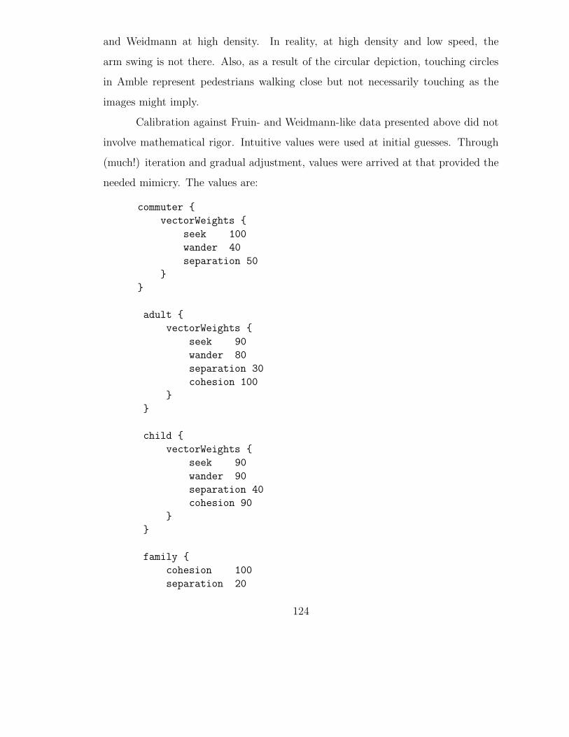
and Weidmann at high density. In reality, at high density and low speed, the

arm swing is not there. Also, as a result of the circular depiction, touching circles

in Amble represent pedestrians walking close but not necessarily touching as the

images might imply.

Calibration against Fruin- and Weidmann-like data presented above did not

involve mathematical rigor. Intuitive values were used at initial guesses. Through

(much!) iteration and gradual adjustment, values were arrived at that provided the

needed mimicry. The values are:

commuter {

vectorWeights {

seek 100

wander 40

separation 50

}

}

adult {

vectorWeights {

seek 90

wander 80

separation 30

cohesion 100

}

}

child {

vectorWeights {

seek 90

wander 90

separation 40

cohesion 90

}

}

family {

cohesion 100

separation 20

124

}

Notice that single people, named commuter in the formal language snippet

above, have no cohesion, are slightly more goal driven than families, and have much

less randomness to their walk. As compared to adults, children wander a little more,

have stronger group cohesion, yet also have willingness to explore more on occasion.

The adult weightings were chosen so that when no children are present, there is a

tendency to walk closely. With the addition of additional group members, however,

that tendency is quickly overcome to some degree.

The values above calibrate the model for the situations studied, similar to

those presented in following sections, that is, situations where people are calmly

walking, occasionally attracted or repulsed by objects in the environment. For panic

situations or evacuations, calibration values would almost certainly be different,

probably little wander, greater family cohesion, less inter-adult cohesion, and no

separation. However, these guesses must be borne out by calibration. One strength

of the model is the flexibility to support such different goals. It is easy to conceive

of using additional velocity vectors and more complex decision making as well.

5.5.2 Validation

Calibration now guarantees that the basic properties of pedestrian movement

are modeled. However, the most important aspect of the pedestrian model, and

hence the Amble software implementation, is the emergent behavior which is not

easily calibrated. Validation takes the testing a step further and compares the

predicted results of simulated scenarios to real situations. In the following scenarios,

sinks are drawn as double edged circles and sources as single edged. This makes it

clear where people are coming from and headed to, and is helpful when viewing still

images rather than the animated simulation.

125

Figure 5.18: Azrieli shopping mall.

5.5.2.1 Scenario 1

The Azrieli Shopping Mall in Israel is used for the first scenario. It is a

heavily fortified structure, and likely as a result has a rather simple floor plan as

seen in Figure 5.18. The photographed portion of the shopping mall is roughly

rectangular in area with store entrances at regular intervals. There are additionally

two kiosks in the center of the mall as well as benches at either end. The Amble

simulation shown in Figure 5.19 displays the mall’s floor plan. Pedestrian behaviors

are used as determined by calibration. However, properties for sources and sinks, as

well as attractiveness of stores and benches, must be determined for this particular

scenario. Certain aspects of all scenarios are necessarily unique and cannot be

126

Figure 5.19: Azrieli simulation.

determined by general calibration. In this case, level of service is good. Sources,

therefore, probabilistically generate traffic at an appropriate rate. Based on the

photo, attraction to stores is estimated by a simple division of number of interested

people in photo by the total number of shoppers. Qualitatively, results in Figure 5.19

display close correlation to the photo. Exact duplication of real life will of course

not happen because of the stochastic nature of the simulation. Notice, however,

two shoppers at the bottom of the simulated scenario sitting on the bench. As

individuals rather than a group, they sit close but not too much so as seen in the

photo. Similarly, a group of 5 simulated pedestrians window shops at the lower

kiosk, just as we see a group of teenage girls shopping at the real kiosk. In this

127

case, the simulated group at the same kiosk stand close to each other, the result of

calibration, as the real girls do.

While the figure captures a representative instant of simulation, tabular mea-

surements are helpful to validate that the simulation prediction is reliable over time.

Measured properties used for validation are walking speed, density, and level of ser-

vice. Vehicular traffic measurements often include gap length because of the one

dimensional nature of vehicular travel. The two dimensional movement of pedes-

trians in open areas, however, makes this measurement less meaningful. Density

is a more useful measure. Calibration is used as previously described to charac-

terize general behavior. Validation uses these settings, but it is then necessary to

model the scenario by characterizing the environment. Physical layout is needed,

but also pedestrian entry and exit counts so that the simulator sources can generate

pedestrians at the correct rate.

The photographed area is approximately 12 m by 32 m in area, and contains

twelve stores and two kiosks. The area at the time of the photograph contains 55

shoppers, yielding a density of 0.16 people per square meter. In terms of Fruin’s

levels of service (Table 5.2), the measurement corresponds to Level of Service C, with

pedestrians having an average walking speed of about 1.2 m/s. On average, about

2 people per second are entering or leaving the modeled area. No data is available

regarding how popular one store is versus another, so an assumption is made that

all stores are equally attractive to shoppers and the kiosks slightly less so simply

because they are smaller. A pedestrian in the area has a 1 in 14 chance of choosing

a particular store and from observation, about 20% to 25% of the shoppers have one

of the stores in the area as a destination. For the simulation set up, this makes a

store appealing to each shopper with a probability of about 0.25/14 = 0.018. About

fifteen percent of the population observed shops singly, and the rest in small groups

of varying sizes fairly evenly distributed in groups of twos, threes, and fours, with

128

0

0.2

0.4

0.6

0.8

1

1.2

1.4

1 2 3 4 5 6 7 8 9 10

Spee

d(m

/s)

Sample Number

PredictedObserved

Figure 5.20: Azrieli pedestrian speed validation.

larger groups rarely seen.

Using the above data to set properties via the formal language of Section 5.3,

the scenario pictured in Figure 5.19 is created. Summarizing the sequence to this

point, interpersonal behavior was calibrated, this particular situation’s characteris-

tics observed and captured in the formal language description, and the results pre-

dicted by simulation can now be compared to observation for validation. Figure 5.20

shows speed measurements, or samples, taken every 30 seconds during simulation.

Initial speeds are higher because the simulated area is just becoming populated with

simulated shoppers. Eventually, there is close correlation to the expected 1.2 m/s

speed, though Amble shows slightly higher speeds. The somewhat higher speed is

expected because calibration showed the same for relatively low densities. Similarly,

129

0

0.02

0.04

0.06

0.08

0.1

0.12

0.14

0.16

0.18

0.2

1 2 3 4 5 6 7 8 9 10

Den

sity

(ped

./m

2)

Sample Number

MeasuredObserved

Figure 5.21: Azrieli pedestrian density validation.

in Figure 5.21 density measurements are sampled every 30 seconds. Again, the ini-

tial sample or two show the lower measurements due to initial population of the

region. Afterwards, the density fluctuates somewhat but remains in the expected

range. The density also shows that a similar level of service exists throughout the

run.

The graphs display history and progression of the simulation, and are mea-

surements of the simulator state at that instant. Figure 5.19 presents one of those

instants. Both qualitatively and quantitatively, the scenario validates the simulator.

5.5.2.2 Scenario 2

In this scenario, the Amazonas Shopping Mall in Manaus, Brazil is used

as shown in Figure 5.22. This is different from the previous scenario in a couple

ways. For one, the layout is slightly more complex. Notice how the mall area

130

Figure 5.22: Amazonas shopping mall.

flares outwards. Additionally, store fronts have large glass windows attracting more

window shopping. The simulated scenario, then, must model windows not as plain

walls, but as areas that can attract pedestrians. They are drawn with dashed lines

in Figure 5.23. Notice in the figure that coincidentally there are shoppers at the

mid-left window shopping as in the photograph. The benches in the middle of the

mall have also attracted some simulated pedestrians, and the average level of service

is comparable in photo and simulation. As in the first scenario, we again see how

group members congregate more tightly than non-groups.

As in the previous validation scenario, after first studying a typical frame of

the ongoing simulation it is helpful to study speed and density trends over time.

The visible area of the lower floor of mall area is approximately 14 m by 20 m, or

280 m2. Because there are 28 people, density works out to be 0.10 people per square

meter. This is about 3.2 m of radial space, or a Fruin level of service of A or B,

131

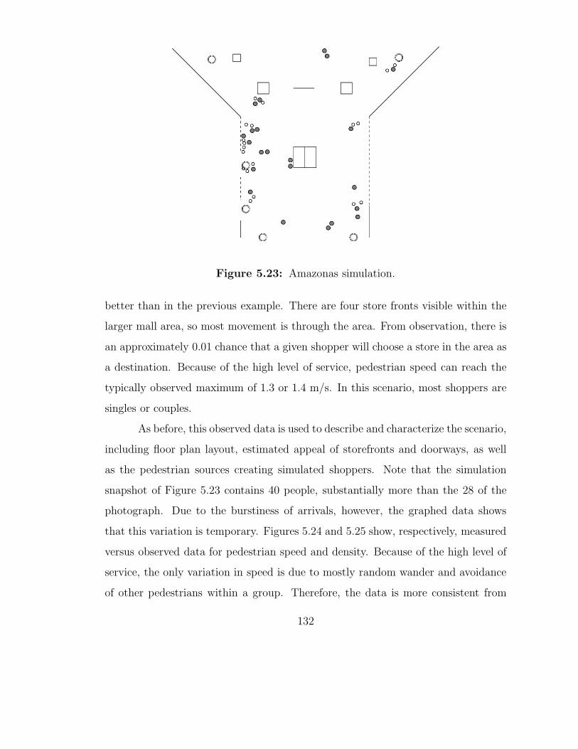
Figure 5.23: Amazonas simulation.

better than in the previous example. There are four store fronts visible within the

larger mall area, so most movement is through the area. From observation, there is

an approximately 0.01 chance that a given shopper will choose a store in the area as

a destination. Because of the high level of service, pedestrian speed can reach the

typically observed maximum of 1.3 or 1.4 m/s. In this scenario, most shoppers are

singles or couples.

As before, this observed data is used to describe and characterize the scenario,

including floor plan layout, estimated appeal of storefronts and doorways, as well

as the pedestrian sources creating simulated shoppers. Note that the simulation

snapshot of Figure 5.23 contains 40 people, substantially more than the 28 of the

photograph. Due to the burstiness of arrivals, however, the graphed data shows

that this variation is temporary. Figures 5.24 and 5.25 show, respectively, measured

versus observed data for pedestrian speed and density. Because of the high level of

service, the only variation in speed is due to mostly random wander and avoidance

of other pedestrians within a group. Therefore, the data is more consistent from

132

0

0.2

0.4

0.6

0.8

1

1.2

1.4

1 2 3 4 5 6 7 8 9 10

Spee

d(m

/s)

Sample Number

MeasuredObserved

Figure 5.24: Amazonas pedestrian speed validation.

sample to sample. Even the occasional bursts of higher density are still far enough

within the bounds of high levels of service that they don’t appreciably affect speed.

5.5.2.3 Scenario 3

The Forum Bornova in Izmir, Turkey is used in this final scenario and one

area of the mall is shown in the photograph of Figure 5.26. The design goal of this

shopping center is to give it the feel of a small Mediterranean village. As such, the

walkways are irregular and straight lines avoided when possible. There is also a fo-

cus on outdoor activity. The two-story, pink Starbuck’s coffee shop provides outdoor

seating under umbrellas. Pools of water provide decoration while channeling pedes-

trian traffic. Figure 5.27 shows the modeled scenario where the collection of three

coffee tables has been replaced by a single pentagon, approximating the footprint of

133

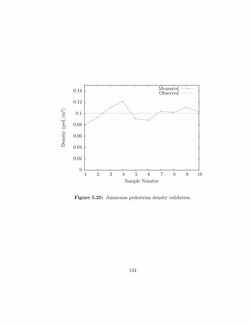
0

0.02

0.04

0.06

0.08

0.1

0.12

0.14

1 2 3 4 5 6 7 8 9 10

Den

sity

(ped

./m

2)

Sample Number

MeasuredObserved

Figure 5.25: Amazonas pedestrian density validation.

134

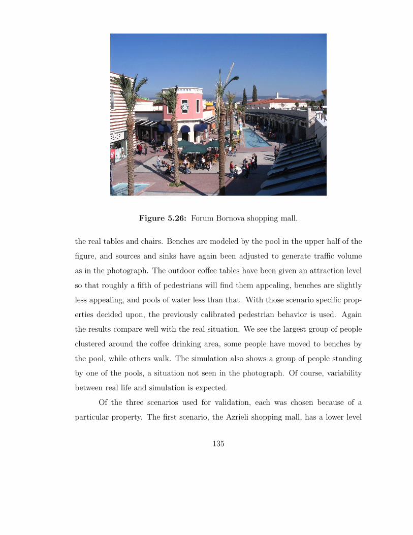
Figure 5.26: Forum Bornova shopping mall.

the real tables and chairs. Benches are modeled by the pool in the upper half of the

figure, and sources and sinks have again been adjusted to generate traffic volume

as in the photograph. The outdoor coffee tables have been given an attraction level

so that roughly a fifth of pedestrians will find them appealing, benches are slightly

less appealing, and pools of water less than that. With those scenario specific prop-

erties decided upon, the previously calibrated pedestrian behavior is used. Again

the results compare well with the real situation. We see the largest group of people

clustered around the coffee drinking area, some people have moved to benches by

the pool, while others walk. The simulation also shows a group of people standing

by one of the pools, a situation not seen in the photograph. Of course, variability

between real life and simulation is expected.

Of the three scenarios used for validation, each was chosen because of a

particular property. The first scenario, the Azrieli shopping mall, has a lower level

135

Figure 5.27: Forum Bornova simulation.

of service, probably because it is located in skyscrapers having a high density of

occupants. The Amazonas shopping mall during the time of study offers a very high

level of service. The Forum Bornova simulation is interesting because it is designed

to offer pedestrian areas that draw people outdoors. The photograph shows many

people outdoors and a simple division of people by square footage would suggest a

lower level of service. Over half the people, however, are seated at tables or benches

and so there is a higher level of service for those walking; a density of approximately

0.11 for people walking. At the lower end of a Fruin level of service A or higher end

of B, measured walking speed is, as in the last scenario, around 1.3 m/s. The same

procedure is followed as outlined in the previous two examples. Measurements are

used to create an Amble formal language file that describes the scenario. Where

measured data is unavailable, estimates are used, and the simulation is run.

There is one notable difference is characterizing this scenario, and that is the

136

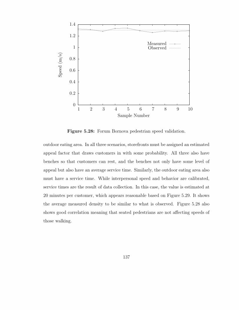
0

0.2

0.4

0.6

0.8

1

1.2

1.4

1 2 3 4 5 6 7 8 9 10

Spee

d(m

/s)

Sample Number

MeasuredObserved

Figure 5.28: Forum Bornova pedestrian speed validation.

outdoor eating area. In all three scenarios, storefronts must be assigned an estimated

appeal factor that draws customers in with some probability. All three also have

benches so that customers can rest, and the benches not only have some level of

appeal but also have an average service time. Similarly, the outdoor eating area also

must have a service time. While interpersonal speed and behavior are calibrated,

service times are the result of data collection. In this case, the value is estimated at

20 minutes per customer, which appears reasonable based on Figure 5.29. It shows

the average measured density to be similar to what is observed. Figure 5.28 also

shows good correlation meaning that seated pedestrians are not affecting speeds of

those walking.

137

0

0.02

0.04

0.06

0.08

0.1

0.12

0.14

1 2 3 4 5 6 7 8 9 10

Den

sity

(ped

./m

2)

Sample Number

MeasuredObserved

Figure 5.29: Forum Bornova pedestrian density validation.

138

5.6 Summary

This chapter has described how the mathematical model of pedestrian move-

ment was implemented in software. An implementation of this magnitude involves

too many details to exhaustively describe, but the most important aspects of the ob-

ject oriented nature of the software were presented. The source code not described

is mainly related to presentation on the screen, animation, and the “glue” to hold

it all together and support communication between the objects. In total, the Java

source code is approximately 10,000 lines.

The code was first shown to be intuitively correct by using examples that

tested its ability for simple steering, group steering, learning, obstacle avoidance,

and scheduling. Next real life scenarios were modeled so that the model parameter

values could be adjusted to closely mimic the scenario. With several situations

showing good correlation between model and reality, Amble predictions are expected

to be reliable.

The programming implementation has been a one person effort and there

are many areas for improvement and enhancement. General enhancements of the

user interface could include editing capabilities to more easily draw walls; describe

sources, sinks, and obstacles; and define and describe agent types. It would also be

better to use normalized coordinates and speeds rather than reference everything

to the modeler specified coordinates of the environment. Similarly, better support

should be implemented for large pedestrian areas that can’t be completely displayed

on the computer screen. Because the focus of the research has been the model rather

than the implementation, it is expected that the implementation is not fully devel-

oped. But even the model itself can be enhanced. It would be especially interesting

to let agents learn from other agents and see what new effects on emergent behavior

it might yield. This would be similar to the simulations of bees and ants as in, for

instance, [BDT99]. In the case of Amble, when a group of pedestrians sees other

139

groups returning from a failed trip, e.g., discovery of a dead end, they could transfer

that information from the more knowledgeable agents to themselves, mimicking ei-

ther observation or verbal communication. Related to this, a study of how changing

behavior parameters affects agent and ultimately system-wide emergent behavior

would be worthwhile. Calibration would be easier with a better understanding of

how simulated behavioral traits interact with each other. (It might even be possible

to compare studies of trait interaction of simulated pedestrians with real people to

see if there is any correlation.)

In summary, Amble offers the modeler more flexibility in scenario set up and

more reliability in predicted results than current simulators described in Chapter 2.

Because this model more closely mimics human behavior, its results tend to be more

in line with reality.

140

Chapter 6

CONCLUSIONS

A pedestrian model is valuable because it saves the engineer, urban planner,

or architect time and work during the design or renovation of pedestrian areas and

ultimately prevents costly mistakes. This is true, however, only if the model is

both reliable and provides detailed enough results. A model using dots to model

people moving cannot be used to study arm swing in a confined area, while a model

studying gait length offers more detail than needed for evacuation studies. As a

result, different models fill different niches. But in addition, all models are limited

by the effects of their simplification of the modeled process.

The model presented in the preceding chapters extends previous work by

incorporating simple versions of memory, learning, and social interaction. Social

interaction, in particular, can be controlled or described by manipulating values of

a handful of model parameters. Calibrated results show that the model is reliable in

typical medium to large pedestrian areas like shopping centers or parks. Simulated

pedestrians that learn are useful because they will cluster around information sources

generating similar levels of congestion as in reality. Memory is similarly useful

because only with it can simulated pedestrians find their ways through areas with

an insufficient amount of information, again generating congestion as one would see

in real life. Social interactions play an equally valuable role in simulations of human

behavior. This appears to be the first civil engineering model incorporating all three

properties.

141

It proved difficult at the start of the research to immediately begin developing

a pedestrian model, so work was started first on creating a vehicle model. Initially

the goal was simply to learn how to make a model incorporating movement and

some behavior characteristics. During model development, however, simplifications

in other models were overcome, namely, lack of lane change modeling, and novel

contributions were made. The three rules developed by Nagel and Schrekenberg

were extended by three new rules characterizing behavior involved in lane changes.

Rules were added supporting lane change for speed increase, lane change toward

correct lane as destination approaches, and change of destination when preceding

rules fail. Analysis of the model showed the effects of aggressive and passive lane

change behaviors.

The vehicle model was created using a cellular automaton. That method

could have been used for a pedestrian model, but was somewhat unwieldy when

trying to deal with pedestrians of different sizes. It also was difficult using dis-

crete cells to simulate compression or elimination of free space around pedestrians

during congestion. These and other difficulties could likely have been overcome,

but it proved much easier to use a continuous physics based model. Agent based

modeling additionally was a natural fit to the problem. Implementing the model in

software became a natural progression from model definition. The simulator, Am-

ble, developed using Java is not a finished product ready for general purpose use,

but it clearly demonstrates that the model can indeed be implemented in software.

The formal language used to describe environment, agent types, and agent behavior

make model calibration as straightforward as editing an input file. Pedestrian mod-

eling is an area far from complete, but the model presented in this thesis brings the

field forward a step, as future models will continue to do by building off this and

other work.

142

BIBLIOGRAPHY

[ABM+03] Craig Anderson, Marlon Boarnet, Tracy McMillan, Mariela Alfonzo,and Kristen Day. Walking and automobile traffic near schools: Data tosupport an evaluation of school pedestrian safety programs. In Trans-portation Research Board 82nd Annual Meeting, volume 82, 2003. Cd-rom publication.

[AOT+03] Takeo Adachi, Toshiya Okabe, Muraleetharan Thambiah, Ken’etsuUchida, Toru Hagiwara, and Sei’ichi Kagaya. Analysis on the influenceof mobility space changes on user attitudes to urban infrastructure im-provement. In Transportation Research Board 82nd Annual Meeting,volume 82, 2003. Cd-rom publication.

[BA98] V. J. Blue and J. L. Adler. Emergent fundamental pedestrian flows fromcellular automata microsimulation. Transportation Research Record,1644:29–36, 1998.

[BA01] V.J. Blue and J.L. Adler. Cellular automata microsimulation for model-ing bi-directional pedestrian walkways. Transportation Research Board,B(35):293–312, 2001.

[BDT99] E. Bonabeau, M. Dorigo, and G. Theraulaz. Swarm Intelligence. OxfordUniversity Press, 1999.

[Bur97] Dan Burden. Walking, bicycling and livable cities [video]. Local Gov-ernment Commission (www.lgc.org), 1414K St., Ste. 250, Sacramento,CA 95814, (916)-448-1198, 1997.

[CGB03] Xuehao Chu, Martin Guttenplan, and Mike Baltes. Why people crosswhere they do, the role of the street environment. In TransportationResearch Board 82nd Annual Meeting, volume 82, 2003. Cd-rom publi-cation.

[Cho56] Noam Chomsky. Three models for the description of language. Infor-mation Theory IEEE Transactions, 2(3):113–124, 1956.

143

[Chu02] Xuehao Chu. A nested logit model of pedestrian street-crossing behav-ior. In 49th Annual North American Meetings of the Regional ScienceAssociation International, pages 3–10, November 2002.

[CJC01] Wayne D. Cottrell, H. Joseph Perrin Jr., and Bhargava RamaChilukuri. Literature Review of Pedestrian-Vehicle Crashes and Anal-ysis of Pedestrian-Vehicle Crashes in Utah. Evaluating and ImprovingPedestrian Safety in Utah, Interim Report No. 2, UTL-0701-44, Uni-versity of Utah., July 2001.

[CP03] Wayne D. Cottrell and Dharminder Pal. Evaluation of pedestrian dataneeds and collection efforts. In Transportation Research Board 82ndAnnual Meeting, volume 82, 2003. Cd-rom publication.

[Daa02] Winnie Daamen. Simped: A pedestrian simulation tool for large pedes-trian areas. In Proceedings of the European Simulation InteroperabilityWorkshop, pages 1–11, 2002.

[Daa04] Winnie Daamen. Modelling passenger flows in public transportation fa-cilities. Ph.D. dissertation, Delft University of Technology, The Nether-lands, 2004.

[DCG59] R. B. Potts D. C. Gazis, R. Herman. Car-following theory of steadystate flow. Operations Research, 7(4):499–505, 1959.

[DDS03] Gary A. Davis, Sujay Davuluri, and Kate Sanderson. A vehi-cle/pedestrian collision model for neighborhood traffic control. InTransportation Research Board 82nd Annual Meeting, volume 82, 2003.Cd-rom publication.

[DH03] Winnie Daamen and Serge P. Hoogendoorn. Experimental research ofpedestrian walking behavior. In Transportation Research Board 82ndAnnual Meeting, volume 82, 2003. Cd-rom publication.

[DT99] Marco Dorigo and Guy Theraulaz. Swarm Intelligence: From Naturalto Artificial Systems. ISBN 0-19-513159-2, 1999.

[DW83] Martin D. Davis and Elaine J. Weyuker. Computability, Complexity,and Languages. Academic Press, 1983.

[Eck06] Bruce Eckel. Thinking in Java. Prentice Hall, 4th edition, 2006.

[EM03] Michelle Ernst and Barbara McCann. Mean streets 2000: Pedestriansafety, health, and transportation spending. Technical report, SurfaceTransportation Policy Project, San Francisco, CA, 2003.

144

[Fru71] John J. Fruin. Pedestrian Planning and Design. Metropolitan Associa-tion of Urban Designers and Environmental Planners, New York, 1971.

[Gar70] Martin Gardner. Mathematical games: The fantastic combinations ofjohn conway’s new solitaire game “life”. Scientific American, 223:120–123, October 1970.

[HB02] Serge P. Hoogendoorn and Piet H. L. Bovy. Normative pedestrian be-haviour theory and modelling. In Michael A. P. Taylor, editor, Trans-portation and Traffic Theory, pages 219–245. Oxford: Pergamon, Else-vier science, 2002.

[HDB03] Serge P. Hoogendoorn, Winnie Daamen, and Piet H. L. Bovy. Extract-ing microscopic pedestrian characteristics from video data results fromexperimental research into pedestrian walking behavior. In Transporta-tion Research Board 82nd Annual Meeting, volume 82, 2003. Cd-rompublication.

[HFV00] Dirk Helbing, Ills Farkas, and Tams Vicsek. Simulating dynamical fea-tures of escape panic. Nature, pages 487–490, September 2000.

[Hoo03] Serge P. Hoogendoorn. Microscopic simulation of pedestrian flows. InTransportation Research Board 82nd Annual Meeting, volume 82, 2003.Cd-rom publication.

[Ins08] Sante Fe Institute. Swarm. http://www.swarm.org, 2008.

[JGL03] Charlotta Johansson, Per Grder, and Lars Leden. Towards vision zeroat zebra crossings - a case study in malm, sweden on traffic safety andmobility for children and elderly. In Transportation Research Board82nd Annual Meeting, volume 82, 2003. Cd-rom publication.

[Jia98] B. Jiang. Multi-agent simulations for pedestrian crowds. In EuropeanSimulation Symposium, Simulation Technology Science and Art, pages383–387, 1998.

[KKWH98] R. Kula, J. Kerridge, A. Wills, and J. Hine. Pedflow: Development of anautonomous agent model of pedestrian flow. In European SimulationSymposium, Simulation Technology Science and Art, pages 383–387,1998.

[KL01] Richard E. Killingsworth and Jean Lamming. Development and pub-lic health; could our development patterns be affecting our personalhealth? Urban Land Institute, pages 12–17, July 2001.

145

[Kno75] R. L. Knoblauch. Urban pedestrian accident countermeasures experi-mental evaluation volume ii: Accident studies. National Highway Traf-fic Safety Administration and Federal Highway Administration, DOTHS-801:346–347, February 1975.

[Knu64] Donald E Knuth. Backus normal form vs. backus naur form. Commu-nications of the ACM, 7(12):735–736, 1964.

[KS06] Tobias Kretz and Michael Schrekenberg. Moore and more and sym-metry. In Pedestrian and Evacuation Dynamics 2005, pages 297–308,2006.

[Lit61] J. D. C. Little. A proof of the queueing formula l = λ w. OperationsResearch, 9:383–387, 1961.

[Lit03] Todd Alexander Litman. Economic value of walkability. In Transporta-tion Research Board 82nd Annual Meeting, volume 82, 2003. Cd-rompublication.

[LYZ05] J. Li, L. Yang, and D. Zhao. Simulation of bi-direction pedestrianmovement in corridor. Physica A, 354:619–628, 2005.

[Mar98] M. J. Markowski. Design and Analysis of Wireless Real-Time Data LinkLayer Protocols. Ph.D. dissertation, University of Delaware, Newark,DE, 1998.

[MCD96] B. Moulin and B. Cabib-Draa. An overview of distributed artificialintelligence. In G. O’hare and N. Jennings, editors, Foundations ofDistributed Artificial Intelligence, pages 3–55. John Wiley and Sons,1996.

[MK04] Michael Markowski and Shinya Kikuchi. Simulating pedestrian inter-actions. In Proceedings of the ASCE Annual Meeting and Symposium,pages 52–56, 2004.

[MN00] M. Muramatsu and T. Nagatani. Jamming transition in two-dimensional pedestrian traffic. Physica A, 275:281–291, 2000.

[NS92] K. Nagel and M. Schrekenberg. A cellular automaton model for freewaytraffic. In Journal de Physique I, pages 2221–2229, 1992.

[Nwa96] H. S. Nwana. Software agents: An overview. The Knowledge Engineer-ing Review, 11(3):205–244, 1996.

146

[PP01] C. S. Papacostas and P. D. Prevedouros. Transportation Engineeringand Planning. Prentice Hall, 3rd edition, 2001.

[PTLS02] G.J. Perez, G. Tapang, M. Lim, and C. Saloma. Streaming, disruptiveinterference and power-law behavior in the exit dynamics of confinedpedestrians. Physica A, 312:609–618, 2002.

[PV05] Alan Penn and Laura S. Vaughan. Pedestrian movement and spatialdesign. Passenger Terminal World Annual, pages 122–125, 2005.

[Rey87] Craig W. Reynolds. Flocks, herds, and schools: A distributed be-havioral model. In ACM SIGGRAPH Conference Proceedings, volume21(4), pages 25–34, 1987.

[Seb07] Robert W. Sebesta. Concepts of Programming Languages. AddisonWesley, 8th edition, 2007.

[SKdF03] Sheila Sarkar, Christine Kaschade, and Fabio de Faria. How well canchild pedestrians estimate potential traffic hazards? In Transporta-tion Research Board 82nd Annual Meeting, volume 82, 2003. Cd-rompublication.

[Sti00] Keith Still. Crowd Dynamics. Ph.D. dissertation, University of War-wick, UK, 2000.

[SUBW03] Dazhi Sun, Satish V. S. K. Ukkusuri, Rahim F. Benekohal, and S. TravisWaller. Modeling of motorist-pedestrian interaction at uncontrolledmid-block crosswalks. In Transportation Research Board 82nd AnnualMeeting, volume 82, 2003. Cd-rom publication.

[Tar01] Mohammed S. Tarawneh. Evaluation of pedestrian speed in Jordan withinvestigation of some contributing factors. Journal of Safety Research,32(2):229–236, 2001.

[TBdS06] Marcelo C. Toyama, Ana L. C. Bazzan, and Roberto da Silva. Anagent-based simulation of pedestrian dynamics: from lane formation toauditorium evacuation. In AAMAS, pages 108–110, 2006.

[Vir98] Mark R. Virkler. Signal coordination benefits for pedestrians. In Trans-portation Research Record, volume 1636, pages 77–82, 1998.

[vNB66] J. von Neumann and A. W. Burks. Theory of Self-reproducing Au-tomata. University of Illinois Press, 1966.

147

[WA98] Paul H. Wright and Normak J. Ashford. Transportation EngineeringPlanning and Design. Prentice Hall, 4th edition, 1998.

[Wei93] Ulrich Weidmann. Transporttechnik der fußganger. Schriftenreihe desInstituts fur Verkehrsplanung, Transporttechnik, Straßen- und Eisen-bahnbau, 90:87–88, 1993.

[WH88] Whyte William H. City, Rediscovering the Center. Doubleday, NewYork, 1988.

[WKHK00] Alex Willis, Robert Kukla, J. Hine, and Jon Kerridge. Developing thebehavioural rules for an agent-based model of pedestrian movement. InProceedings of the European Transport Conference, pages 69–80, 2000.

[Wol02] Stephen Wolfram. A New Kind of Science. Wolfram Media, 2002.

[WS01] J. Wahle and M. Schrekenberg. A multi-agent system for on-line sim-ulations based on real-world traffic data. In Proceedings of the HawaiiInternational Conference on System Science, pages 3037–3045. IEEEComputer Society, 2001.

[YKN07] Kazuhiro Yamamotoa, Satoshi Kokuboa, and Katsuhiro Nishinari. Sim-ulation for pedestrian dynamics by real-coded cellular automata (rca).Physica A, 379(2):654–660, 2007.

[Zac01] John Zacharias. Pedestrian behavior and perception in urban walkingenvironments. Journal of Planning Literature, 16(1):3–18, 2001.

148