Embed Size (px)
Citation preview

Modeling Basket Credit Default Swaps with Default Contagion
Helen Haworth∗
[email protected] Reisinger
The Nomura Centre for Quantitative FinanceOCIAM Mathematical Institute
Oxford University24-29 St Giles
Oxford, OX1 3LBEngland
Tel. +44 1865 280612
December 2006
∗This work is kindly supported by Nomura and the EPSRC.
1

Executive Summary
The specification of a realistic dependence structure is key to the pricing of multi-name creditderivatives. We value small kth-to-default CDS baskets in the presence of asset correlationand default contagion. Using a first-passage framework, firm values are modeled as correlatedgeometric Brownian motions with exponential default thresholds. Idiosyncratic links betweencompanies are incorporated through a contagion mechanism whereby a default event leadsto jumps in volatility at related entities. Our framework allows for default causality and isextremely flexible, enabling us to evaluate the spread impact of firm value correlations andcredit contagion for symmetric and asymmetric baskets.
Keywords
Basket credit default swaps, default dependence, credit risk, correlation, contagion, first-passage model.
2
1 Introduction
The effects of a corporate default are usually felt far beyond the individual firm in question,rippling through the market, causing changes in the credit spreads of related companies.Generally these would be increases in spreads of companies deemed to be exposed to similarrisks, but could also be manifest as tightening spreads of companies likely to benefit fromthe default. In this paper, we specify a multi-firm structural credit model with a dependencestructure incorporating firm-value correlations and this type of contagious default behavior.
Broadly speaking, credit weakness, ratings downgrades and ultimately corporate default canoccur in three main ways. Firstly, a company may be adversely affected for reasons specificto that company alone (e.g. poor financial management). Secondly, credit weakness mayoccur due to a factor or factors impacting multiple companies – whether in the form of acyclical influence related to the economy, or a market-wide shock such as an earthquake orterrorist attack. Finally, companies are related through ties, some of which are real (e.g. atrade-creditor agreement), others of which are purely a matter of perception – for example thefear of accounting fraud. Credit dependence then occurs primarily through two mechanisms– either as a direct consequence of a common driving factor, or due to inter-company ties.
In order to incorporate such a dependence structure into the structural framework, we considera firm-value model with default as the first hitting time of an exponential barrier. Firm assetsare modeled as correlated geometric Brownian motions and default by one firm has a knock-on impact on remaining companies in the form of a jump in firm volatility – contagion. Inthis way, we are able to capture the two facets of the dependence structure. The correlationin firm values reflects a longer-term common driving influence on corporate strength whilstdefault contagion represents a direct link between the fortunes of both companies. The resultis a model that allows for default causality and is asymmetric with regard to default risk, asignificant improvement on prior models.
Until recently, the vast majority of work on the structural model focused on the case of a singlefirm, with two popular commercial packages, Moody’s KMV and CreditGradesTM motivatedby the single-firm structural model1. Giesecke (2004), Schonbucher (2003) and Lando (2004)provide a good introduction to structural models, their development since first introduced byMerton (1974), and their traditional place within credit modeling. Though not so straight-forward mathematically, structural models are far more grounded in economic fundamentalsthan many other models and thus form a good starting point for a realistic description ofcredit dynamics. Very little, however, has been published for multiple companies, with themarket mainly focused on copulas or conditionally independent factor models2 in the multi-variate case. In two exceptions, Hull and White (2000) use Monte Carlo simulation to valuea basket CDS in a structural-type model whilst Zhou (2001) calculates default correlationsfor two correlated Brownian motions.
Existing models used in the market suffer many limitations and as problems have arisen withtheir widespread use, structural models have started to see some renewed interest. Hull et al.
1Further details of these approaches can be found at www.moodyskmv.com and in Finger et al. (2002),respectively.
2For a good overview of the use of copulas in finance, see Cherubini et al. (2004); Schonbucher (2003)provides a useful summary and references for factor models.
3

(2005) price CDO tranches in a structural framework where assets are driven by a commonfactor. In another approach, Luciano and Schoutens (2005), Moosbrucker (2006) and Baxter(2006) assume that firm values are driven by Levy processes rather than geometric Brownianmotions and model credit derivatives using Variance Gamma processes. Haworth et al. (2006)build on the approach of Zhou (2001) to derive closed-form solutions for corporate bond yieldsin the presence of default contagion and correlated two-firm basket credit default swaps.
This paper is a generalisation of the analytical approach of Haworth et al. (2006), incor-porating a more flexible and realistic specification of the default contagion mechanism andallowing for rapid valuation of three-firm credit default swap (CDS) baskets. It is organisedas follows. Section 2 contains a description of the model and its numerical implementation,with results for two-firm baskets considered in detail in Section 3. The two-company model isextended in Section 4 to allow the impact of default contagion to dissipate over time. Resultsfor three-firm baskets are then illustrated in Section 5 and the current numerical limitationsof the model in higher dimensions are discussed. Section 6 outlines the extension to a generalm-factor framework and we conclude with a discussion of future areas of interest.
2 Modeling Methodology
2.1 Setup
We consider n companies with firm values Vi, i = 1 . . . n. For each company, firm value isassumed to follow a geometric Brownian motion, with default as the first time that the valueof the firm hits a lower default barrier bi(t). As in Merton (1974) and Black and Cox (1976),we assume that a firm’s value can be constructed from tradable securities and so under therisk-neutral pricing measure, for i = 1, . . . , n,
dVi(t) = (rf − qi)Vi(t) dt + σiVi(t) dWi(t) (1)
where the risk-free rate, rf , dividend yields, qi, and volatilities, σi, are constants, Wi(t) areBrownian motions and cov(Wi(t),Wj(t)) = ρijt for constant correlations ρij , i, j = 1, . . . , n.
We assume that each company has an exponential default barrier, reflecting the existence ofdebt covenants, and denote the default barrier for company i by
bi(t) = Kie−γi(T−t)
for constants Ki, γi. T represents the maturity of the product of interest or, more generally,the length of the time period under consideration.
We are interested in default probabilities – for example, the probability that a given firmdefaults by a given time horizon, or the probability that a certain number of firms default ina specified period. If Ω represents the event of interest, V is the vector of firm values and Lis the infinitesimal generator of (1) then we can calculate the probability of the event Ω bysolving
LU =∂U
∂t+
n∑
i=1
βiVi∂U
∂Vi+
12
n∑
i,j=1
aijViVj∂2U
∂Vi∂Vj= 0 (2)
U(V, T ) = IΩ(V(T )) (3)
4

for the function U(V, t), since by the Feynman-Kac formula,
U(v, t) = E IΩ(V(T ))|V(t) = v = P (V(T ) ∈ Ω|V(t) = v) ,
where IΩ denotes the indicator function of the event Ω and
βi = rf − qi (4)aij = ρijσiσj . (5)
2.2 Introducing Credit Contagion
As specified so far, the dependence structure is driven purely by the correlation in firm values.Default by a company has no direct impact on the behavior of the remaining companies; thereis no credit or default contagion. This we incorporate by allowing the values of aij in (2), tojump on default. If company i defaults, this causes a jump in the volatilities, σj , of firms j,i 6= j, thereby introducing credit contagion. Subsequent defaults cause further jumps in thevolatilities of firms that are still ‘alive’.
By relating the size and direction of the jump in σj to the correlation between companies iand j, both positive and negative effects and differing degrees of contagion can be incorpo-rated. The result is a dependence structure incorporating both mechanisms described in theintroduction. Exposure to common factors arises through the specification of correlated firmvalue processes in (1), whilst the contagion mechanism reflects the existence of a network ofinter-company links.
Asymmetric ties are easy to incorporate, allowing some companies to have greater influencethan others, in the vein of work done by Jarrow and Yu (2001) in which ‘primary’ companiesimpact ‘secondary’ companies but not vice versa3. Our model is flexible enough to specify anarbitrary number of different relationships between companies.
2.3 Implementation
We solve (2) backwards in time on [0, T ] × Rn+ using a finite-difference method with Crank
Nicolson time-stepping and a multigrid solver as in Reisinger and Wittum (2004). To definethe initial condition, we specify the coefficients in equation (2) such that once a company hitsits default barrier it remains constant. In other words, we set each firm’s drift and volatilityto zero on its barrier and define new coefficients βi and aij ,
βi(Vi, t) := βiIVi(t) > bi(t) aij(Vi, Vj , t) := aijIVi(t) > bi(t), Vj(t) > bj(t) . (6)
In this way, when a firm reaches its default barrier and defaults, its value does not change,enabling us to count the number of companies whose values are less than or equal to theirdefault barriers4 at a given point in time and define the initial condition in (3) according to
3A ‘primary’ company is likely to be larger with a greater market impact than a ‘secondary’ company. Forexample Microsoft or General Motors compared to a small, local IT or auto component manufacturer.
4The barrier is an increasing function, so its value at maturity will be greater than or equal the value atwhich default occurred.
5

the value we want to calculate. For example, if we want the probability that all companiessurvive, we set the initial condition to be one when there are no companies at or below theirdefault barriers, and zero elsewhere. If we want the probability of k defaults, we set it to beone when k companies are valued at or below their barriers, zero otherwise.
The event that the k ≤ n companies i1, . . . , ik default by time T (but no others) is given bythe set
Ωi1,...,ik =Vij (T ) ≤ bij (T ) for j = 1, . . . , k and Vij (T ) > bij (T ) otherwise
and the set Ωk corresponding to exactly k companies defaulting in [0, T ] is
Ωk =⋃
I⊂1,...,n, |I|=k
ΩI .
We can therefore calculate the probability of k defaults in [0, T ] by solving (2) with U(V, T ) =IΩk
(V(T )).
To illustrate our approach, we incorporate default contagion by assuming that if company idefaults, the volatility of company j, i 6= j, jumps by
σj → σjFρij (7)
for some constant F ≥ 1. In other words,
σj(V, t) =
σj if Vi(t) > bi(t), Vj(t) > bj(t)σjF
ρij if Vi(t) ≤ bi(t), Vj(t) > bj(t)0 if Vj(t) ≤ bj(t)
(8)
In this way, a company positively correlated with the defaulting company experiences anincrease in volatility, and hence an increase in credit spreads, whilst a negatively correlatedcompany becomes less volatile and consequently less risky. The degree of correlation has animpact on the size of the jump in volatility, and by changing the value of F , default canbe assumed to have a bigger or smaller influence on the strength of the remaining company.This formulation is intuitive and serves to illustrate the impact that company relationshipscan have on credit spreads. However, (7) is of course just one of many possible specificationsof the contagion mechanism that could be used and others could be handled similarly. Asubsequent default by a firm k /∈ i, j would be incorporated in exactly the same way with
σj → σjFρij → σjF
ρijF ρkj ,
and so on for any further defaults.
In the two dimensional case, we can also solve the problem analytically on the boundarysince in the event of default by one company, the equation reduces to a one-dimensionalhitting probability. Rather than solving the whole problem numerically as outlined above,it is therefore possible to define the boundary conditions analytically as the solution of theremaining one-firm problem. This approach is outlined in more detail in Section 4, where itis applied to the case of contagion that decays over time. Extension of this method to threeor more dimensions could be done recursively, but would be considerably more involved.
6

2.4 CDS Spread Calculation
The buyer of a kth-to-default credit default swap (CDS) on a basket of n companies paysa premium, the CDS spread, for the life of the CDS – until maturity or the kth default,whichever happens first. In the event of default by the kth underlying reference company, thebuyer receives a default payment and the contract terminates. Writing τk for the time of thekth default, if recovery on default is R, and the protection buyer makes continuous spreadpayments, c, on a par value K, then the discounted spread payment (DSP) and discounteddefault payment (DDP) on the kth-to-default basket are
DSP = cK
∫ T
0e−rf sP(τk > s) ds
DDP = (1−R)K∫ T
0e−rf sP(s ≤ τk ≤ s + ds) ds
= (1−R)K∫ T
0−e−rf s ∂
∂sP(τk > s) ds
= (1−R)K
1− e−rf TP(τk > T )− rf
∫ T
0e−rf sP(τk > s) ds
,
giving market kth-to-default CDS spread, ck,
ck =(1−R)
1− e−rf TP(τk > T )− ∫ T
0 rfe−rf sP(τk > s) ds
∫ T0 e−rf sP(τk > s) ds
. (9)
In addition to calculating default and survival probabilities using (2), we can simultaneouslyevaluate the integral over time of a function of the default or survival probability of interest.By setting the initial condition to be one if less than k companies default, we can thereforecalculate P(τk > T ) and
∫ T0 e−rf sP(τk > s) ds, and hence kth-to-default credit default swap
spreads by (9).
3 Two-Firm Results
We begin by illustrating the use and flexibility of the model for the case of two companies,allowing us to highlight its main attributes. By modifying the initial condition, we are ableto calculate a number of different survival probabilities and first and second-to-default CDSspreads.
Our results are generated using a regular grid with 210 + 1 grid-points in each direction and200 time-steps. On an Intel Xeon CPU 3.5 Ghz x2 machine, it takes about eight minutesto generate default probabilities for a given value of correlation at 200 points in a ten-yearperiod. Comparing default probabilities with those obtained analytically in Haworth et al.(2006), using 10 uniform refinements and 200 time-steps gives results accurate to five decimalplaces. We have gone for accuracy over speed; to generate the same results accurate to threedecimal places takes just thirty seconds.
7
As a measure of company strength we consider initial credit quality, defined as initial firmvalue, Vi(0), divided by the initial level of the barrier, bi(0). As would be expected, as initialcredit quality declines, spreads widen significantly. An indicative scaled distance to default,1σi
log(Vi(0)/bi(0)), for parameter values of σi = 0.2 and initial credit quality of 2 is then 3.5.An upward jump in a company’s volatility due to default by a related firm therefore reducesthe distance to default, leading to higher default probabilities and hence greater spreads.
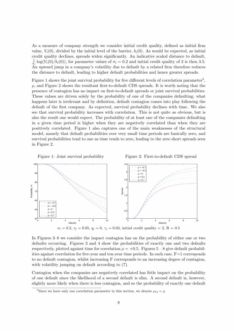
Figure 1 shows the joint survival probability for five different levels of correlation parameter5,ρ, and Figure 2 shows the resultant first-to-default CDS spreads. It is worth noting that thepresence of contagion has no impact on first-to-default spreads or joint survival probabilities.These values are driven solely by the probability of one of the companies defaulting; whathappens later is irrelevant and by definition, default contagion comes into play following thedefault of the first company. As expected, survival probability declines with time. We alsosee that survival probability increases with correlation. This is not quite as obvious, but isalso the result one would expect. The probability of at least one of the companies defaultingin a given time period is higher when they are negatively correlated than when they arepositively correlated. Figure 1 also captures one of the main weaknesses of the structuralmodel, namely that default probabilities over very small time periods are basically zero, andsurvival probabilities tend to one as time tends to zero, leading to the zero short spreads seenin Figure 2.
Figure 1: Joint survival probability
0 2 4 6 8 1040
50
60
70
80
90
100
Maturity
Pro
babi
lity,
%
ρ = −0.7
ρ = −0.3
ρ = 0
ρ = 0.3
ρ = 0.7
Figure 2: First-to-default CDS spread
0 2 4 6 8 100
0.5
1
1.5
2
2.5
3
3.5
Maturity
Spr
ead
ρ = −0.7
ρ = −0.3
ρ = 0
ρ = 0.3
ρ = 0.7
σi = 0.2, rf = 0.05, qi = 0, γi = 0.03, initial credit quality = 2, R = 0.5
In Figures 3–8 we consider the impact contagion has on the probability of either one or twodefaults occurring. Figures 3 and 4 show the probabilities of exactly one and two defaultsrespectively, plotted against time for correlation ρ = +0.5. Figures 5 – 8 give default probabil-ities against correlation for five-year and ten-year time periods. In each case, F=1 correspondsto no default contagion, whilst increasing F corresponds to an increasing degree of contagion,with volatility jumping on default according to (7).
Contagion when the companies are negatively correlated has little impact on the probabilityof one default since the likelihood of a second default is slim. A second default is, however,slightly more likely when there is less contagion, and so the probability of exactly one default
5Since we have only one correlation parameter in this section, we denote ρ12 = ρ.
8

Figure 3: Probability of 1 default
0 2 4 6 8 100
5
10
15
20
25
30
Maturity
Pro
babi
lity
(%)
F=1F=2F=3F=4
Figure 4: Probability of 2 defaults
0 2 4 6 8 100
5
10
15
20
25
Maturity
Pro
babi
lity
(%)
F=1F=2F=3F=4
Default probabilities for ρ = +0.5σi = 0.2, rf = 0.05, qi = 0, γi = 0.03, initial credit quality = 2
is slightly lower for lower values of F. When the companies are positively correlated, contagionhas a greater impact, and since a second default is more likely for higher F, the probabilityof one default is lower for higher F, while the probability of two defaults is higher.
Since zero correlation corresponds to no contagion, all curves cross at this point. The prob-ability of a second default being higher for positive correlation and contagion, and lower fornegative correlation and contagion, explains the position of the curves relative to one an-other. In Figure 7, for example, for negative correlation, a greater degree of contagion meansa second default is less likely, so the probability of exactly one default is greater for highervalues of F. Contrastingly, a second default is more likely with higher F for positive valuesof correlation and so the probability of one default decreases with increasing F for positivecorrelation. The same argument explains the results for the probability of two defaults.
Figure 5: Probability of 1 default
−1 −0.5 0 0.5 1 0
5
10
15
20
25
Correlation
Pro
babi
lity
(%)
F=1F=2F=3F=4
Figure 6: Probability of 2 defaults
−1 −0.5 0 0.5 1 0
2
4
6
8
10
12
14
Correlation
Pro
babi
lity
(%)
F=1F=2F=3F=4
Five-year default probabilitiesσi = 0.2, rf = 0.05, qi = 0, γi = 0.03, initial credit quality = 2
9

Figure 7: Probability of 1 default
−1 −0.5 0 0.5 1 0
10
20
30
40
50
60
Correlation
Pro
babi
lity
(%)
F=1F=2F=3F=4
Figure 8: Probability of 2 defaults
−1 −0.5 0 0.5 1 0
5
10
15
20
25
30
35
Correlation
Pro
babi
lity
(%)
F=1F=2F=3F=4
Ten-year default probabilitiesσi = 0.2, rf = 0.05, qi = 0, γi = 0.03, initial credit quality = 2
In Figures 6 and 8 we see that the probability of two defaults peaks for a value of ρ < 1for higher values of F. The same effect is evident and better highlighted in Figures 9 and 10which illustrate the impact of correlation and contagion on the expected number of defaultsover five and ten years.
Figure 9: 5 years
−1 −0.5 0 0.5 1 0.23
0.24
0.25
0.26
0.27
0.28
0.29
0.3
0.31
Correlation
Num
ber
F=1F=2F=3F=4
Figure 10: 10 years
−1 −0.5 0 0.5 1 0.5
0.52
0.54
0.56
0.58
0.6
0.62
0.64
0.66
0.68
0.7
Correlation
Num
ber
F=1F=2F=3F=4
Expected number of defaultsσi = 0.2, rf = 0.05, qi = 0, γi = 0.03, initial credit quality = 2
For a given value of ρ, the higher F is, the greater the impact the contagion has on theexpected number of defaults, as expected. However, the greatest impact occurs for values ofρ = ρ± where −1 < ρ− < 0 and 0 < ρ+ < 1, and not for ρ = ±1. As ρ increases, there areconflicting influences on default probabilities. With increasing correlation, the probabilityof a default decreases, however, if one occurs, the presence of contagion then means that asecond default is much more likely for high positive values of ρ and unlikely for negative valuesof ρ. For ρ− < ρ < ρ+, the presence of contagion is the driving factor with spreads increasingwith correlation. For correlation nearer ±1, the probability of there being a default in the
10

first place for contagion to have an effect is more important. In other words, contagion hasthe biggest impact for ρ ∈ (ρ−, ρ+), the most likely levels to occur in reality.
As illustrated in Figures 9 and 10, in the absence of contagion (F=1), the expected number ofdefaults is independent of the level of correlation. This follows immediately from the linearityof the expectation operator, and denoting the default indicator process for firm i by Ni, canbe calculated directly from
E(Number of defaults) =2∑
i=1
P(Ni = 1).
Writing
Yi(t) = ln(
Vi(t)Vi(0)
e−γit
)= αit + σiWi(t)
αi = rf − qi − γi − 12σ2
i
Bi = ln(
bi(0)Vi(0)
),
then
P(Ni = 1) = 1− P(Y i(t) ≥ Bi)
= Φ(
Bi − αit
σi
√t
)+ e2αiBi/σ2
i Φ(
Bi + αit
σi
√t
),
providing an easy way to check the accuracy of our numerical results6.
Figures 11 and 12 show the impact of contagion on five and ten-year second-to-default CDSspreads for different values of correlation. Again, we see the same form, with spreads higherin the presence of contagion for positive correlation and lower for negative correlation, witha peak for some 0 < ρ < 1 for positive values of contagion. The more likely a second defaultis to occur, the riskier the default swap and the greater the spread. Figures 13 and 14 showthe same results against maturity for ρ = ±1/2. It is clear from both sets of graphs that theexistence and nature of both firm-value correlation and default contagion can have a largeimpact on CDS spreads.
Our framework for incorporating contagion is flexible enough to enable us to assume thatonly default by certain companies leads to contagion. This we illustrate in Figures 15 and16 for the case of two correlated companies, only one of which directly influences the other.For F=2 and F=4, we compare the case in which bankruptcy of either company causes ajump in volatility at the remaining company (labeled ‘Double’ in the graphs) to the case inwhich only one company impacts the other (labeled ‘Single’ in the graphs). In the latter case,if company one defaults, the volatility of company two jumps, but if company two defaults,company one carries on as usual, its volatility unaffected by the default.
Results are as we would expect with asymmetric contagion having less impact on spreads.Considering the relative impact of F=2 Double (symmetric contagion) and F=4 Single (asym-metric contagion) also highlights the non-linear relationship between changes in volatility and
6Results in Figures 9 and 10 are accurate to five decimal places using ten refinements and 200 time-steps.
11

Figure 11: 5-year 2nd-to-default CDS
−1 −0.5 0 0.5 1 0
0.2
0.4
0.6
0.8
1
1.2
1.4
Correlation
Spr
ead
F=1F=2F=3F=4
Figure 12: 10-year 2nd-to-default CDS
−1 −0.5 0 0.5 1 0
0.2
0.4
0.6
0.8
1
1.2
1.4
1.6
1.8
Correlation
Spr
ead
F=1F=2F=3F=4
σi = 0.2, rf = 0.05, qi = 0, γi = 0.03, initial credit quality = 2, R = 0.5
Figure 13: ρ = −0.5
0 2 4 6 8 100
0.02
0.04
0.06
0.08
0.1
0.12
0.14
Maturity
Spr
ead
F=1F=2F=3F=4
Figure 14: ρ = +0.5
0 2 4 6 8 100
0.2
0.4
0.6
0.8
1
1.2
1.4
Maturity
Spr
ead
F=1F=2F=3F=4
Second-to-default spreads with credit contagionσi = 0.2, rf = 0.05, qi = 0, γi = 0.03, initial credit quality = 2, R = 0.5
12

Figure 15: ρ = −0.5
0 2 4 6 8 100
0.02
0.04
0.06
0.08
0.1
0.12
0.14
Maturity
Spr
ead
F=1F=2 SingleF=2 DoubleF=4 SingleF=4 Double
Figure 16: ρ = +0.5
0 2 4 6 8 100
0.2
0.4
0.6
0.8
1
1.2
1.4
Maturity
Spr
ead
F=1F=2 SingleF=2 DoubleF=4 SingleF=4 Double
Second-to-default spreads with asymmetric credit contagionσi = 0.2, rf = 0.05, qi = 0, γi = 0.03, initial credit quality = 2, R = 0.5
changes in spreads. For ρ = −0.5, symmetric contagion with F=2 has more spread impactthan asymmetric contagion with F=4. The reverse is true for ρ = +0.5.
Calculating the probability that a given company defaults is also straightforward in thisframework and so we can consider the impact of correlated firm values and contagion on thelevel of default contagion using
Corr[N1(t), N2(t)] =E[N1(t) ·N2(t)]− E[N1(t)] · E[N2(t)]√
Var[N1(t)] ·Var[N2(t)]. (10)
with Ni the default indicator process for firm i as before, and
E[Ni(t)] = P(Ni(t) = 1)Var[Ni(t)] = P(Ni(t) = 1) · [1− P(Ni(t) = 1)]
E[N1(t) ·N2(t)] = E[N1(t)] + E[N2(t)]− P(N1(t) = 1 or N2(t) = 1).
Zhou (2001) examines the impact of firm value correlation and firm credit quality on defaultcorrelation in the non-contagion setting. Figures 17 and 18 illustrate the impact of contagionfor five and ten-year horizons. As expected, the presence of credit contagion increases therange of possible default correlations. When asset correlation is positive, contagion increasesdefault correlation, and when it is negative, contagion causes default correlation to becomemore negative.
In Figures 19 and 20 we illustrate the term structure of default correlation, with and withoutcontagion. Results can be compared with Figure 1 in Zhou (2001). Using identical parametersto Zhou, we are able to exactly replicate his results using our method. Of note, for ourparameter values, over the ten-year time horizon shown, we see no peak in the magnitudeof default correlation. This is as a result of the lower value we assign to firm volatility –0.2 compared to 0.4 in Zhou’s work. As he explains, the magnitude of default correlationdeclines over the longer-term since beyond a certain point, the event of non-default becomesidiosyncratic. The effect of reducing volatility or increasing initial credit quality is to movethe peak in default correlation further out – beyond ten years in our case.
13
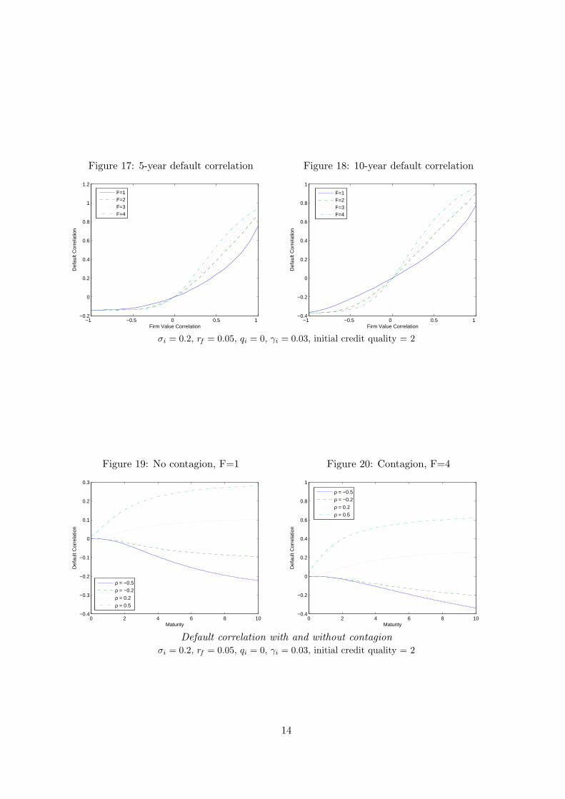
Figure 17: 5-year default correlation
−1 −0.5 0 0.5 1 −0.2
0
0.2
0.4
0.6
0.8
1
1.2
Firm Value Correlation
Def
ault
Cor
rela
tion
F=1F=2F=3F=4
Figure 18: 10-year default correlation
−1 −0.5 0 0.5 1 −0.4
−0.2
0
0.2
0.4
0.6
0.8
1
Firm Value Correlation
Def
ault
Cor
rela
tion
F=1F=2F=3F=4
σi = 0.2, rf = 0.05, qi = 0, γi = 0.03, initial credit quality = 2
Figure 19: No contagion, F=1
0 2 4 6 8 10−0.4
−0.3
−0.2
−0.1
0
0.1
0.2
0.3
Maturity
Def
ault
Cor
rela
tion
ρ = −0.5
ρ = −0.2
ρ = 0.2
ρ = 0.5
Figure 20: Contagion, F=4
0 2 4 6 8 10−0.4
−0.2
0
0.2
0.4
0.6
0.8
1
Maturity
Def
ault
Cor
rela
tion
ρ = −0.5
ρ = −0.2
ρ = 0.2
ρ = 0.5
Default correlation with and without contagionσi = 0.2, rf = 0.05, qi = 0, γi = 0.03, initial credit quality = 2
14

4 Contagion with Decay
Currently, with contagion as specified by (7), the knock-on effect of a default has a lastingimpact on remaining companies. Once a firm’s volatility jumps to a new level, it staysthere forever. This is not necessarily particularly realistic unless the default event serves topermanently change the corporate environment. Rather, it is more usual for contagion totake the form of a decaying spike in spreads or volatility. In the absence of a second defaultor more news, spreads tend to trend back towards their original level over time.
In the event of default by company i, we can incorporate this behavior into our model byhaving company j’s volatility jump according to
σj → σj(1 + ∆ije−ζ(t−τi)). (11)
In this way, volatility jumps by an amount ∆ij , which can depend on the identity of thedefaulting company, and then trends exponentially back to its original level, at a rate de-termined by the parameter ζ. τi denotes the default time of firm i and j 6= i. For basketsof n > 2 companies, the impact of a second or subsequent default would be incorporatedsimilarly. For example, for k /∈ i, j, if company i defaulted at time τi and then company kdefaulted at time τk > τi, the impact on the volatility of firm j would be
σj → σj(1 + ∆ije−ζ(t−τi)) for τi ≤ t ≤ τk
→ σj(1 + ∆ije−ζ(t−τi))(1 + ∆kje
−ζ(t−τk)) for t ≥ τk.
Since the extent and direction of the jump in volatility is likely to depend on the identityof the firms in question, it makes sense for ∆ij to vary, and also for it to be possible for∆ij 6= ∆ji so that there is an asymmetry in the default impact of companies on one another.Similarly, ζ could be allowed to depend on the firm identities.
Davis and Lo (2001) allow for a similar effect in their model of infectious defaults. Theyconsider large homogeneous portfolios with two risk states – normal and enhanced. Defaultby one of the companies causes the hazard rate of all remaining companies to jump to anelevated level where it remains for an exponentially distributed length of time before returningto its original level. In their framework there are therefore two jumps in the hazard rate,marking the beginning and the end of the enhanced-risk state. Here, we assume an initialjump in volatility on default, the effect of which then dissipates over time.
Assuming that company i is the first company to default, the volatilities of the remainingfirms as given by (11) are then time-dependent, σj(t), j 6= i for t ≥ τi. As outlined inWilmott (1998), we can remove the time-dependence by replacing σ2
j (t) with its average overthe remaining time-to-maturity, σ2
j , where
σ2j =
1T − τi
∫ T−τi
0σ2
j (s) ds
=σ2
j
T − τi
∫ T−τi
0
(1 + 2∆ije
−ζs + ∆2ije
−2ζs)
ds
= σ2j +
2∆ijσ2j
ζ(T − τi)
(1− e−ζ(T−τi)
)+
σ2j ∆
2ij
2ζ(T − τi)
(1− e−2ζ(T−τi)
).
15

In the case of a two-firm basket, we can then solve the PDE (2), by breaking the time periodinto two since the equation decouples on the boundary. We consider the usual two-firmproblem on [0, τi] and a one-company problem on [τi, T ]. By standard first passage theory,as given in Musiela and Rutkowski (1998), the probability that company j survives and doesnot fall below its default threshold before maturity T given that company i defaults at timeτi < T is
Φ(
Xj(τi) + αj(T − τi)σj
√T − τi
)− e−2αjXj(τi)/σ2
j Φ(−Xj(τi) + αj(T − τi)
σj
√T − τi
), (12)
where αj = rf − qj − γj − σ2j /2 and Xj(t) = ln
(Vj(t)e−γjt/bj(0)
).
We then solve (2) on [0, τi] exactly as before, subject to additional boundary conditionsat Xi(t) = 0 given by (12). By modifying the initial condition and specifying the boundaryconditions according to whether we are interested in company j surviving or defaulting, we areable to calculate a range of default probabilities as before, and asymmetric default contagioncan be easily incorporated.
For consistency with the framework in Section 3, we set ∆ = F ρ− 1, so that the initial jumpin volatility is driven by both the degree of contagion, F , and the correlation between firmvalues, as before7. By specifying the process in this manner we can directly compare resultswith and without decay as shown in Figures 21 – 28.
In Figures 21 – 24, we consider results for no contagion (F=1, ζ = 0), contagion but no decay(F=4, ζ = 0) and contagion with varying rates of decay (F=4, ζ = 0.5, 2, 4, &8). Valuesof ζ of 8, 4 and 2 correspond to volatility reverting to its pre-default level over roughly sixmonths, one year and two years, respectively. For the purpose of comparison, we also includethe fairly extreme case of ζ = 0.5 for which the effects of the default take nearly ten years todissipate. In practice for a company’s default to have such a lasting impact, it would haveto have been a key company in the sector or market of interest, or a particularly momentousdefault. The possible bankruptcy of General Motors and the fall-out following the Enrondebacle spring to mind as incidences that might lead to such a long-drawn out settling downof spreads.
Figures 21 and 22 show the probability of one and two defaults, respectively, for a ten-yearperiod. We see that results with a decay in default contagion, ζ > 0, have the same form andlie closer to results with no contagion (shown by the solid black line) than those with a highdegree of permanent contagion, ζ = 0. As ζ increases, the rate at which the contagion effectsdissipate increases and probabilities tend more quickly towards their non-contagion level.
Since the rate of decay is exponential, it makes sense that the impact of the contagion is fairlylimited when compared to the situation in which the jump in volatility is permanent. Thatsaid, as we see from the 2nd-to-default spreads in Figures 23 and 24, the effect is still largeenough to warrant attention. For highly correlated companies, even if the knock-on impactof the default dissipates in six months (ζ = 8), spreads are five to ten basis points higher withcontagion. The spread impact of contagion for negative values of ρ is considerably lower thanfor positive ρ. This is because for ρ < 0 contagion serves to reduce volatility and increasingvolatility by a given amount (e.g. from 0.2 to 0.3) has a much bigger impact on spreads thanreducing volatility by the same amount (0.2 to 0.1).
7As in Section 3, we denote ρ12 = ρ and so ∆ is the same for both companies.
16

Figure 21: Probability of 1 default
−1 −0.5 0 0.5 1 0
10
20
30
40
50
60
Correlation
Pro
babi
lity,
%
ζ = 0ζ = 0.5ζ = 2ζ = 4ζ = 8No contagion
Figure 22: Probability of 2 defaults
−1 −0.5 0 0.5 1 0
5
10
15
20
25
30
35
Correlation
Pro
babi
lity,
%
ζ = 0
ζ = 0.5
ζ = 2
ζ = 4
ζ = 8No contagion
Ten-year default probabilities with decaying contagionσi = 0.2, rf = 0.05, qi = 0, γi = 0.03, initial credit quality = 2
Figure 23: 10-year 2nd-to-default CDS
−1 −0.5 0 0.5 1 0
0.2
0.4
0.6
0.8
1
1.2
1.4
1.6
1.8
Correlation
Spr
ead
ζ = 0
ζ = 0.5
ζ = 2
ζ = 4
ζ = 8No contagion
Figure 24: Spread curve for ρ = 0.5
0 2 4 6 8 100
0.2
0.4
0.6
0.8
1
1.2
1.4
Maturity
Spr
ead
ζ = 0
ζ = 0.5
ζ = 2
ζ = 4
ζ = 8No contagion
2nd-to-default CDS spreads with decaying contagionσi = 0.2, rf = 0.05, qi = 0, γi = 0.03, initial credit quality = 2, R = 0.5
17

Figures 25 – 28 show the direct impact of contagion on spreads for positive values of corre-lation. Figures 25 – 26 give results for ρ = 0.5, Figures 27 – 28 for ρ = 0.75. In each casewe illustrate the extra spread in basis points (1/100ths of a percent) for 2nd-to-default CDSswith contagion compared to the base case of correlated firm values but no default contagion.For reference, in the absence of contagion, the five-year spread with ρ = 0.5 is 38 basis points,whilst for ρ = 0.75 it is 63 basis points. The extra spreads we are seeing due to the existenceof contagion are therefore of a meaningful size.
Figure 25:
0 2 4 6 8 100
10
20
30
40
50
60
70
Maturity
Ext
ra S
prea
d, b
asis
poi
nts
ζ = 0
ζ = 0.5
ζ = 2
ζ = 4
ζ = 8
Figure 26:
0 2 4 6 8 100
2
4
6
8
10
12
14
16
18
Maturity
Ext
ra S
prea
d, b
asis
poi
nts
ζ = 2
ζ = 4
ζ = 8
Additional spread on 2nd-to-default CDS due to contagion, ρ = 0.5σi = 0.2, rf = 0.05, qi = 0, γi = 0.03, initial credit quality = 2, R = 0.5
Figure 27:
0 2 4 6 8 100
10
20
30
40
50
60
70
80
Maturity
Ext
ra S
prea
d, b
asis
poi
nts
ζ = 0
ζ = 0.5
ζ = 2
ζ = 4
ζ = 8
Figure 28:
0 2 4 6 8 100
5
10
15
20
25
30
35
40
Maturity
Ext
ra S
prea
d, b
asis
poi
nts
ζ = 2
ζ = 4
ζ = 8
Additional spread on 2nd-to-default CDS due to contagion, ρ = 0.75σi = 0.2, rf = 0.05, qi = 0, γi = 0.03, initial credit quality = 2, R = 0.5
From the left hand graphs, we see that when contagion results in a permanent increase involatilities (ζ = 0), spreads increase with maturity – the longer dated the CDS, the greaterthe impact of contagion. This is not the case when the jump in volatility declines over time.As would be expected, the faster the rate of decay, the shorter the maturity of the productthat sees the greatest spread impact, and the earlier we see a peak in the spread difference.
18

This is easier to see in the right hand graphs, Figures 26 and 28. These reproduce the lowerthree curves of the left hand graphs and show clearly the peaks for ζ = 2, 4 and 8. Forρ = 0.75, contagion with ζ = 2 has the greatest impact on spreads for a 4.9-year maturityCDS whilst when ζ = 8, the difference is greatest for a maturity of 3.9 years.
5 Results for Three Firms
Using identical numerical techniques as in Section 3, we can generate kth-to-default spreadsfor baskets of three companies. We begin, as in the two-firm case, by showing results for thejoint survival probability and first-to-default CDS spread in Figures 29 and 30. Comparingwith Figures 1 and 2 for the two-company basket, we see the same shaped curves. As wouldbe expected, survival probabilities are lower and spreads are higher when there are three firmsas the presence of the extra company increases the risk of the product.
Figure 29: Joint survival probability
0 2 4 6 8 1030
40
50
60
70
80
90
100
Maturity
Pro
babi
lity
(%)
ρ = −0.3ρ = 0ρ = 0.2ρ = 0.5
Figure 30: First-to-default CDS spread
0 2 4 6 8 100
0.5
1
1.5
2
2.5
3
3.5
4
4.5
5
Maturity
Spr
ead
ρ = −0.3
ρ = 0
ρ = 0.2
ρ = 0.5
σi = 0.2, rf = 0.05, qi = 0, γi = 0.03, initial credit quality = 2, R = 0.5
In Figures 29 – 34, we are assuming that all three firms have identical characteristics, givenby the parameters shown, and that there is just one correlation variable, ρij = ρ, i 6= j.Considering homogeneous firms in the first instance enables us to see the direct spread impactof changes in correlation and default contagion.
Figures 31 and 32 show second-to-default spreads for various values of correlation, with andwithout contagion. As before, spreads are the same in each case for zero correlation, lower withcontagion for negatively correlated firms and higher with contagion when firms are positivelycorrelated. The same results are illustrated in Figures 33 – 34 for third-to-default spreads.Spreads are greatest for first-to-default products and lowest for third-to-default products, asthey should be.
Finally, in Figures 35 and 36, we provide some results for different correlation structures.In order of increasing spreads, Figure 35 compares first-to-default swap spreads for a two-firm basket with correlation of 0.5 (2D:ρ = 0.5), a three-firm basket with correlation of 0.5between all firms (3D:ρ = 0.5), a three-firm basket with two correlated and one completelyuncorrelated firm (3D:ρ12 = 0.5, ρ23 = ρ13 = 0) and a three-firm basket with positively and
19

Figure 31: No contagion, F=1
0 2 4 6 8 100
0.2
0.4
0.6
0.8
1
1.2
1.4
Maturity
Spr
ead
ρ = −0.3
ρ = 0
ρ = 0.2
ρ = 0.5
Figure 32: Contagion, F=4
0 2 4 6 8 100
0.5
1
1.5
2
2.5
Maturity
Spr
ead
ρ = −0.3
ρ = 0
ρ = 0.2
ρ = 0.5
2nd-to-default CDS spreadsσi = 0.2, rf = 0.05, qi = 0, γi = 0.03, initial credit quality = 2, R = 0.5
Figure 33: No contagion, F=1
0 2 4 6 8 100
0.05
0.1
0.15
0.2
0.25
0.3
0.35
0.4
Maturity
Spr
ead
ρ = −0.3
ρ = 0
ρ = 0.2
ρ = 0.5
Figure 34: Contagion, F=4
0 2 4 6 8 100
0.2
0.4
0.6
0.8
1
1.2
1.4
1.6
1.8
Maturity
Spr
ead
ρ = −0.3
ρ = 0
ρ = 0.2
ρ = 0.5
3rd-to-default CDS spreadsσi = 0.2, rf = 0.05, qi = 0, γi = 0.03, initial credit quality = 2, R = 0.5
20

Figure 35: 1st-to-default CDS spread
0 2 4 6 8 100
0.5
1
1.5
2
2.5
3
3.5
4
4.5
Maturity
Spr
ead
2D: ρ = 0.5
3D: ρ = 0.5
3D: ρ12
= 0.5, ρ23
= ρ13
= 0
3D: ρ12
= 0.5, ρ13
= −0.5,ρ23
= −0.25
Figure 36: 2nd-to-default CDS spread
0 2 4 6 8 100
0.2
0.4
0.6
0.8
1
1.2
1.4
1.6
Maturity
Spr
ead
2D: ρ = 0.5, F=13D: Asymmetrical, F=1
3D: ρ12
= 0.5, F=1
2D: ρ = 0.5, F=43D: Asymmetrical, F=4
3D: ρ12
= 0.5, F=4
σi = 0.2, rf = 0.05, qi = 0, γi = 0.03, initial credit quality = 2, R = 0.53D: Asymmetrical corresponds to ρ12 = 0.5, ρ13 = −0.5, ρ23 = −0.25
3D:ρ12 = 0.5 corresponds to ρ12 = 0.5, ρ23 = ρ13 = 0.
negatively correlated firms (3D:ρ12 = 0.5, ρ13 = −0.5, ρ23 = −0.25). The order is intuitive,but it is interesting to note the relative differences in spreads and the impact that varyingthe correlation structure can have. Figure 36 gives similar results for second-to-default swapspreads, considering, in addition, the impact of contagion (F = 4 versus F = 1). Once again,these graphs highlight the flexibility of the model for investigating the relationship betweenthe dependence structure and spreads.
We are restricted by memory constraints to using a maximum of six refinements in ournumerical evaluation of three-dimensional results. This means that calculations are very fast(the number of refinements is the limiting factor in the accuracy of results rather than thenumber of time-steps) but are not quite as accurate as we would like8. Whilst our numericalmethod is currently not quite accurate enough to be used for pricing three-firm baskets, themodel nonetheless represents a powerful tool for considering the sensitivity of CDS spreadsto assumptions regarding input parameters and the dependence structure.
Incorporating decaying contagion in three (or more) dimensions is not as straightforward asin the two-dimensional case, but could be done recursively, starting with the case when allbar one of the firms have defaulted to define the boundary conditions for the boundary planes(as done in Section 4 for the two-dimensional case), and then solving the two-firm case onthese planes to give the boundary conditions in three-dimensions.
6 General m-Factor Framework
Numerical limitations aside, the framework has the flexibility to enable a very general spec-ification of firm value dynamics and underlying correlation structure. Supposing that firm
8By comparing results for P(τ1 < T ) calculated in the two and three-dimensional case and stressing thesurvival probabilities and integrals used in (9) accordingly, the maximum absolute error was around 10 basispoints, usually much less.
21

values are driven by both a number of macro factors and an idiosyncratic factor, with cor-relation between firms arising from their individual exposures to the macro driving factors,then for n companies, values Vi(t), with idiosyncratic factors Wi(t) and m independent macrodriving processes Yj(t),
dVi(t) = (rf − qi)Vi(t)dt + δiVi(t)dWi(t) +m∑
j=1
γijVi(t)dYj(t)
= βiVi(t)dt +d∑
j=1
ηijVi(t)dZj(t) (13)
where d = m + n, βi = rf − qi,
ηij =
δi & dZj(t) = dWj(t) for 1 ≤ j ≤ n, i = j0 & dZj(t) = dWj(t) for 1 ≤ j ≤ n, i 6= jγi(j−n) & dZj(t) = dY(j−n)(t) for n + 1 ≤ j ≤ d,
and for each i and all j, the Brownian motions Wi(t) and Yj(t) are uncorrelated with oneanother. βi represents the expected growth rate of the value of firm i and the weightings γij
and δi represent the exposure of company i to the various macro and idiosyncratic factors.The larger a given weighting is, the greater that factor’s influence and the potentially morevolatile the company. As before, we assume that company i defaults the first time that itsvalue drops below the level of its default barrier bi(t). Defined in this way, company values canbe considered to be driven by both company-specific and global factors. The latter could, forexample, be at the country, sector or industry level, introducing a rich correlation structurebetween companies.
If V is the vector of firm values, for a function U(V, t), the infinitesimal generator of (13) is
LU =∂U
∂t+
n∑
i=1
βiVi∂U
∂Vi+
12
n∑
i,j=1
aijViVj∂2U
∂Vi∂Vj(14)
where
aijdt =d∑
k,l=1
ηikηjl 〈dZk, dZl〉 , (15)
and 〈dZk, dZl〉 represents the quadratic covariation between dZk and dZl.
Applying the Feynman-Kac formula as before, we can then calculate the probability of kdefaults in [0, T ] by solving
∂U
∂t+
n∑
i=1
βiVi∂U
∂Vi+
12
n∑
i,j=1
aijViVj∂2U
∂Vi∂Vj= 0
U(V, T ) = IΩk(V), (16)
where Ωk is the set corresponding to exactly k companies defaulting in [0, T ].
The basic structure of (13) is related to that considered by Hull et al. (2005) in which thevalue of company i’s assets evolves according to
d ln Vi = µidt + αi(t)σidF (t) +√
1− αi(t)2σidUi(t)
22

for common and idiosyncratic Brownian motions F (t) and Ui(t). The correlation structureis driven by the αi(t)s, which may be either stochastic or time-dependent, but there is nomechanism for introducing any type of default contagion or inter-company ties in their model.
7 Conclusion
We have proposed a numerical approach to modeling firm value dynamics and the defaultevent, enabling valuation of basket credit default swap spreads in a first passage frameworkwith both asset correlation and default contagion. The approach is easy to implement andenables specification of a rich dependence structure incorporating asymmetries and defaultcausality. By modifying the initial condition, there is great flexibility to calculate manydifferent default and survival probabilities of interest, allowing evaluation of kth-to-defaultCDS spreads, the expected number of defaults and default correlations.
Results reiterate the need for credit models to take into account a full dependence structure,with default contagion having a very clear impact on spreads. Whilst the accuracy of thenumerical approach is not quite good enough for pricing baskets of three or more companiesand memory constraints prohibit extension to large baskets using current methodology, themodel could be used as a powerful tool for analysing the spread impact of different dependenceassumptions and parameter values.
The goal remains to extend the approach to cope with bigger baskets in order to price largekth-to-default CDS products and CDO tranches. We have the framework for specifying thedynamics and a realistic dependence structure, but extending the numerics to deal withhigher dimensions has proven elusive using finite difference methods9. Current work includesapplying Monte Carlo techniques to the framework with the goal to model large portfolios ofup to 125 companies by dimension reduction using principal component analysis.
Extending the framework to a non geometric Brownian motion setting would be relativelystraightforward. It would be interesting to see the impact of incorporating stochastic cor-relation or stochastic volatility, although this would raise the added issue of market incom-pleteness. By relating firm correlations or volatilities to a global state variable, it would bepossible to have default correlations depend on the state of the economy as considered byHull et al. (2005), reflecting the fact that defaults tend to be more highly correlated whendefault probabilities are higher. Another desirable extension would be to incorporate jumpsinto the specification of the underlying firm value dynamics to remove the predictable natureof default and the resultant zero short spreads. In all cases, results need to be related to thoseseen in practice, with an evaluation of the ability of different model specifications to explainrealistic spread behavior.
References
M. Baxter. Dynamic modelling of single-name credits and CDO tranches. Nomura FixedIncome Quant Group, 2006.9We tried many techniques to increase the speed and accuracy including sparse grid methods (Reisinger
and Wittum (2004)), coordinate transformations and singularity removal methods, but with limited success.
23

http : //www.nomura.com/resources/europe/pdfs/cdomodelling.pdf.
F. Black and J. Cox. Valuing corporate securities: Some effects of bond indenture provisions.Journal of Finance, 31:351–367, 1976.
U. Cherubini, E. Luciano, and W. Vecchiato. Copula methods in finance. Wiley, 2004.
M. Davis and V. Lo. Modelling default correlation in bond portfolios. Working Paper,Imperial College, London., 2001.http : //www.ma.ic.ac.uk/ mdavis/docs/mastering risk.pdf.
C. Finger, V. Finkelstein, G. Pan, J. Lardy, T. Thomas, and J. Tierney. CreditgradesTM .Technical Document, RiskMetrics Group, Inc., 2002.http : //www.creditgrades.com/resources/pdf/CGtechdoc.pdf.
K. Giesecke. Credit risk modeling and valuation: An introduction. Working Paper, CornellUniversity, 2004.http ://www.stanford.edu/dept/MSandE/people/faculty/giesecke/introduction.pdf.
H. Haworth, C. Reisinger, and W. Shaw. Modelling bonds and credit default swaps using astructural model with contagion. Working paper, Oxford University, 2006.http : //www.maths.ox.ac.uk/~haworthh/Webfiles/2DArticle.pdf.
J. Hull, M. Predescu, and A. White. The valuation of correlation-dependent credit derivativesusing a structural model. Working Paper, University of Toronto, 2005.http ://www.rotman.utoronto.ca/~hull/DownloadablePublications/StructuralModel.pdf.
J. Hull and A. White. Valuing credit default swaps II: Modeling default correlations. WorkingPaper, University of Toronto, 2000.http : //www.stern.nyu.edu/fin/workpapers/papers00/wpa00022.pdf.
R. Jarrow and J. Yu. Counterparty risk and the pricing of defaultable securities. The Journalof Finance, LVI No. 5:1765–1800, 2001.
D. Lando. Credit Risk Modeling: Theory & Applications. Princeton University Press, 2004.
E. Luciano and W. Schoutens. A multivariate jump-driven financial asset model. ICERWorking Paper, 2005.http : //perswww.kuleuven.be/~u0009713/multivg.pdf.
R. Merton. On the pricing of corporate debt: The risk structure of interest rates. Journal ofFinance, 29:449–470, 1974.
T. Moosbrucker. Pricing CDOs with correlated Variance Gamma distributions. WorkingPaper, University of Cologne, 2006.http : //www.fmpm.ch/docs/9th/papers 2006 web/9112b.pdf.
M. Musiela and M. Rutkowski. Martingale Methods in Financial Modelling. Springer, 1998.
C. Reisinger and G. Wittum. On multigrid for anisotropic equations and variational inequal-ities. Computing and Visualization in Science, 7:189–197, 2004.
P.J. Schonbucher. Credit derivatives pricing models. Wiley, 2003.
P. Wilmott. Derivatives: The theory and practice of financial engineering. Wiley, 1998.
24

C. Zhou. An analysis of default correlations and multiple defaults. The Review of FinancialStudies, 14:555–576, 2001.
25


![Bloom Berg, Konikov] Basket Default Swaps](https://img.dokumen.tips/doc/110x75/577d394c1a28ab3a6b997dda/bloom-berg-konikov-basket-default-swaps.jpg)
![[Lehman Brothers] Valuation of Credit Default Swaps](https://img.dokumen.tips/doc/110x75/55cf9895550346d033987d79/lehman-brothers-valuation-of-credit-default-swaps-562533741d6fc.jpg)


