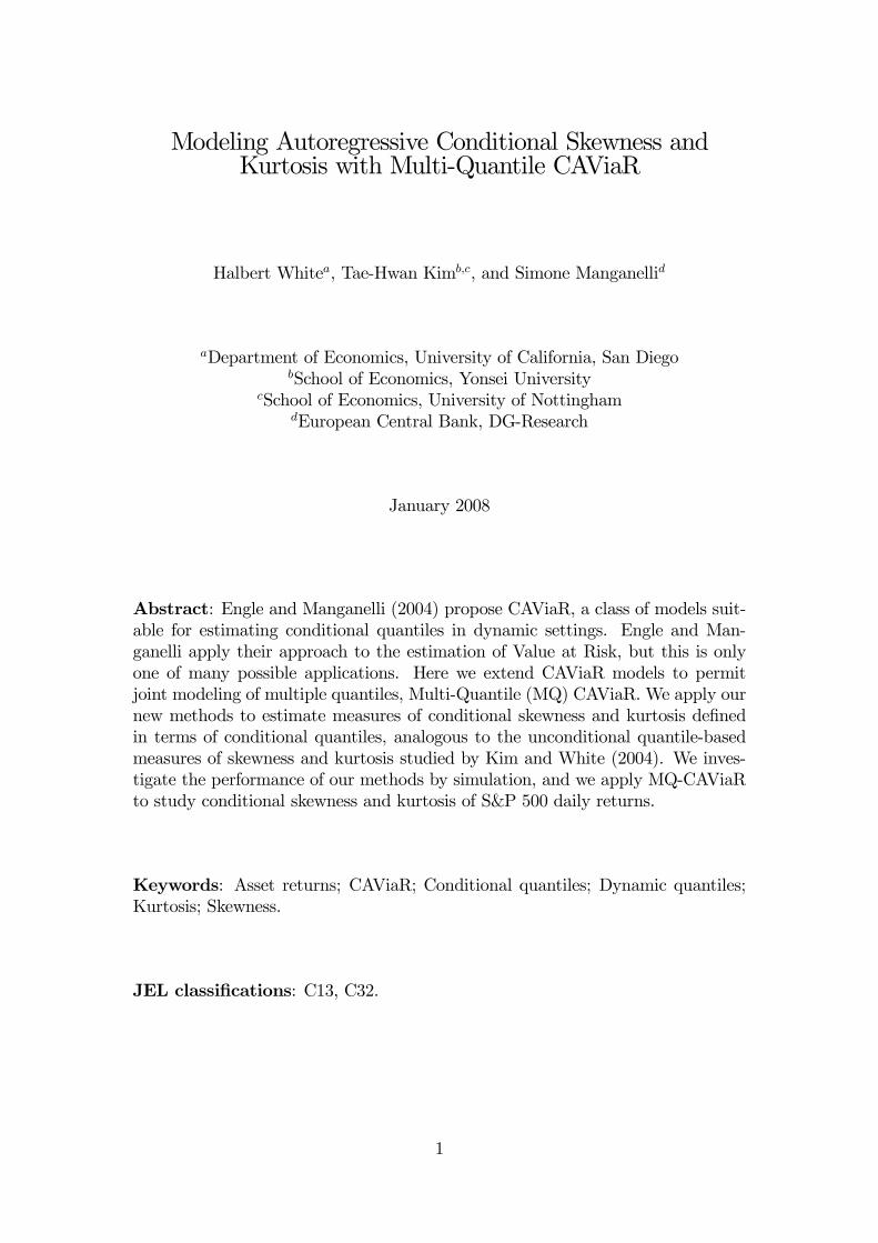
Modeling Autoregressive Conditional Skewness andKurtosis with Multi-Quantile CAViaR

Halbert Whitea, Tae-Hwan Kimb,c, and Simone Manganellid

aDepartment of Economics, University of California, San DiegobSchool of Economics, Yonsei University

cSchool of Economics, University of NottinghamdEuropean Central Bank, DG-Research

January 2008

Abstract: Engle and Manganelli (2004) propose CAViaR, a class of models suit-able for estimating conditional quantiles in dynamic settings. Engle and Man-ganelli apply their approach to the estimation of Value at Risk, but this is onlyone of many possible applications. Here we extend CAViaR models to permitjoint modeling of multiple quantiles, Multi-Quantile (MQ) CAViaR. We apply ournew methods to estimate measures of conditional skewness and kurtosis definedin terms of conditional quantiles, analogous to the unconditional quantile-basedmeasures of skewness and kurtosis studied by Kim and White (2004). We inves-tigate the performance of our methods by simulation, and we apply MQ-CAViaRto study conditional skewness and kurtosis of S&P 500 daily returns.

Keywords: Asset returns; CAViaR; Conditional quantiles; Dynamic quantiles;Kurtosis; Skewness.

JEL classifications: C13, C32.

1

1 Introduction

It is widely recognized that the use of higher moments, such as skewness and kur-

tosis, can be important for improving the performance of various financial models.

Responding to this recognition, researchers and practitioners have started to in-

corporate these higher moments into their models, mostly using the conventional

measures, e.g. the sample skewness and/or the sample kurtosis. Models of con-

ditional counterparts of the sample skewness and the sample kurtosis, based on

extensions of the GARCH model, have also been developed and used; see, for ex-

ample, Leon, Rubio, and Serna (2004). Nevertheless, Kim and White (2004) point

out that because standard measures of skewness and kurtosis are essentially based

on averages, they can be sensitive to one or a few outliers — a regular feature of

financial returns data — making their reliability doubtful.

To deal with this, Kim and White (2004) propose the use of more stable and

robust measures of skewness and kurtosis, based on quantiles rather than averages.

Nevertheless, Kim and White (2004) only discuss unconditional skewness and

kurtosis measures. In this paper, we extend the approach of Kim andWhite (2004)

by proposing conditional quantile-based skewness and kurtosis measures. For this,

we extend Engle and Manganelli’s (2004) univariate CAViaR model to a multi-

quantile version, MQ-CAViaR. This allows for both a general vector autoregressive

structure in the conditional quantiles and the presence of exogenous variables. We

then use the MQ-CAViaR model to specify conditional versions of the more robust

skewness and kurtosis measures discussed in Kim and White (2004).

The paper is organized as follows. In Section 2, we develop the MQ-CAViaR

data generating process (DGP). In Section 3, we propose a quasi-maximum likeli-

hood estimator for the MQ-CAViaR process and prove its consistency and asymp-

totic normality. In Section 4, we show how to consistently estimate the asymptotic

variance-covariance matrix of the MQ-CAViaR estimator. Section 5 specifies con-

ditional quantile-based measures of skewness and kurtosis based on MQ-CAViaR

estimates. Section 6 contains an empirical application of our methods to the S&P

500 index. We also report results of a simulation experiment designed to examine

the finite sample behavior of our estimator. Section 7 contains a summary and

concluding remarks. Mathematical proofs are gathered into the Mathematical

Appendix.

2

2 The MQ-CAViaR Process and Model

We consider data generated as a realization of the following stochastic process.

Assumption 1 The sequence (Yt,X 0t) : t = 0,±1,±2, ..., is a stationary and

ergodic stochastic process on the complete probability space (Ω,F , P0), where Ytis a scalar and Xt is a countably dimensioned vector whose first element is one.

Let Ft−1 be the σ-algebra generated by Zt−1 ≡ Xt, (Yt−1,Xt−1), ..., i.e.Ft−1 ≡ σ(Zt−1). We let Ft(y) ≡ P0[Yt < y|Ft−1] define the cumulative distri-

bution function (CDF) of Yt conditional on Ft−1.

Let 0 < θ1 < ... < θp < 1. For j = 1, ..., p, the θjth quantile of Yt conditional

on Ft−1, denoted q∗j,t, is

q∗j,t ≡ infy : Ft(y) = θj, (1)

and if Ft is strictly increasing,

q∗j,t = F−1t (θj).

Alternatively, q∗j,t can be represented asZ q∗j,t

−∞dFt(y) = E[1[Yt≤q∗j,t]|Ft−1] = θj, (2)

where dFt(y) is the Lebesgue-Stieltjes probability density function (PDF) of Ytconditional on Ft−1, corresponding to Ft(y).

Our objective is to jointly estimate the conditional quantile functions q∗j,t, j =

1, 2, ..., p. For this we write q∗t ≡ (q∗1,t, ..., q∗p,t)0 and impose additional appropriatestructure.

First, we ensure that the conditional distribution of Yt is everywhere contin-

uous, with positive density at each conditional quantile of interest, q∗j,t. We let

ft denote the conditional probability density function (PDF) corresponding to Ft.

In stating our next condition (and where helpful elsewhere), we make explicit the

dependence of the conditional CDF Ft on ω by writing Ft(ω, y) in place of Ft(y).

Realized values of the conditional quantiles are correspondingly denoted q∗j,t(ω).

Similarly, we write ft(ω, y) in place of ft(y).

After ensuring this continuity, we impose specific structure on the quantiles of

interest.

Assumption 2 (i) Yt is continuously distributed such that for each t and each

ω ∈ Ω, Ft(ω, ·) and ft(ω, ·) are continuous on R; (ii) For given 0 < θ1 < ... <

3

θp < 1 and q∗j,t as defined above, suppose: (a) For each t and j = 1, ..., p,

ft(ω, q∗j,t(ω)) > 0; (b) For given finite integers k and m, there exist a stationary

ergodic sequence of random k × 1 vectors Ψt, with Ψt measurable−Ft−1, and

real vectors β∗j ≡ (β∗j,1, ..., β∗j,k)0 and γ∗jτ ≡ (γ∗jτ1, ..., γ∗jτp)0 such that for all t andj = 1, ..., p,

q∗j,t = Ψ0tβ∗j +

mXτ=1

q∗0t−τγ∗jτ . (3)

The structure of eq. (3) is a multi-quantile version of the CAViaR process

introduced by Engle and Manganelli (2004). When γ∗jτi = 0 for i 6= j, we have the

standard CAViaR process. Thus, we call processes satisfying our structure "Multi-

Quantile CAViaR" (MQ-CAViaR) processes. For MQ-CAViaR, the number of

relevant lags can differ across the conditional quantiles; this is reflected in the

possibility that for given j, elements of γ∗jτ may be zero for values of τ greater

than some given integer. For notational simplicity, we do not represent m as

depending on j. Nevertheless, by convention, for no τ ≤ m do we have γ∗jτ equal

to the zero vector for all j.

The finitely dimensioned random vectors Ψt may contain lagged values of Yt,

as well as measurable functions of Xt and lagged Xt and Yt. In particular, Ψt may

contain Stinchcombe and White’s (1998) GCR transformations, as discussed in

White (2006).

For a particular quantile, say θj, the coefficients to be estimated are β∗j and

γ∗j ≡ (γ∗0j1, ..., γ∗0jm)

0. Let α∗0j ≡ (β∗0j , γ∗0j ), and write α∗ = (α∗01 , ..., α

∗0p )0, an × 1

vector, where ≡ p(k+mp).We will call α∗ the "MQ-CAViaR coefficient vector."

We estimate α∗ using a correctly specified model of the MQ-CAViaR process.

First, we specify our model.

Assumption 3 LetA be a compact subset ofR . (i) The sequence of functions qt :Ω×A→ Rp is such that for each t and each α ∈ A, qt(·, α) is measurable−Ft−1;

for each t and each ω ∈ Ω, qt(ω, ·) is continuous onA; and for each t and j = 1, ..., p,

qj,t(·, α) = Ψ0tβj +

mXτ=1

qt−τ(·, α)0γjτ .

Next, we impose correct specification and an identification condition. As-

sumption 4(i.a) delivers correct specification by ensuring that the MQ-CAViaR

coefficient vector α∗ belongs to the parameter space, A. This ensures that α∗

optimizes the estimation objective function asymptotically. Assumption 4(i.b) de-

livers identification by ensuring that α∗ is the only such optimizer. In stating the

4

identification condition, we define δj,t(α, α∗) ≡ qj,t(·, α) − qj,t(·, α∗) and use thenorm ||α|| ≡ maxi=1,..., |αi|.

Assumption 4 (i)(a) There exists α∗ ∈ A such that for all t

qt(·, α∗) = q∗t ; (4)

(b) There exists a non-empty set J ⊆ 1, ..., p such that for each > 0 there

exists δ > 0 such that for all α ∈ A with ||α− α∗|| > ,

P [∪j∈J|δj,t(α, α∗)| > δ ] > 0.

Among other things, this identification condition ensures that there is sufficient

variation in the shape of the conditional distribution to support estimation of

a sufficient number (#J) of variation-free conditional quantiles. In particular,

distributions that depend on a given finite number of parameters, say k, will

generally be able to support k variation-free quantiles. For example, the quantiles

of the N(µ, 1) distribution all depend on µ alone, so there is only one "degree of

freedom" for the quantile variation. Similarly the quantiles of scaled and shifted

t−distributions depend on three parameters (location, scale, and kurtosis), sothere are only three "degrees of freedom" for the quantile variation.

3 MQ-CAViaR Estimation: Consistency andAsymptotic Normality

We estimate α∗ by the method of quasi-maximum likelihood. Specifically, we

construct a quasi-maximum likelihood estimator (QMLE) αT as the solution to

the following optimization problem:

minα∈

ST (α) ≡ T−1TXt=1

pX

j=1

ρθj(Yt − qj,t(·, α)), (5)

where ρθ(e) = eψθ(e) is the standard "check function," defined using the usual

quantile step function, ψθ(e) = θ − 1[e≤0]. We thus view

St(α) ≡ −pX

j=1

ρθj(Yt − qj,t(·, α))

as the quasi log-likelihood for observation t. In particular, St(α) is the log-likelihood

of a vector of p independent asymmetric double exponential random variables

5

(see White, 1994, ch. 5.3; Kim and White, 2003; Komunjer, 2005). Because

Yt − qj,t(·, α∗), j = 1, ..., p need not actually have this distribution, the method isquasi maximum likelihood.

We can establish the consistency of αT by applying results of White (1994).

For this we impose the following moment and domination conditions. In stating

this next condition and where convenient elsewhere, we exploit stationarity to

omit explicit reference to all values of t.

Assumption 5 (i) E|Yt| <∞; (ii) let D0,t ≡ maxj=1,...,p supα∈ |qj,t(·, α)|,t = 1, 2, ... . Then E(D0,t) <∞.

We now have conditions sufficient to establish the consistency of αT .

Theorem 1 Suppose that Assumptions 1, 2(i, ii), 3(i), 4(i), and 5(i, ii) hold. ThenαT

a.s.→ α∗.

Next, we establish the asymptotic normality of T 1/2(αT−α∗). We use a methodoriginally proposed by Huber (1967) and later extended by Weiss (1991). We first

sketch the method before providing formal conditions and results.

Huber’s method applies to our estimator αT , provided that αT satisfies the

asymptotic first order conditions

T−1TXt=1

pX

j=1

∇qj,t(·, αT ) ψθj(Yt − qj,t(·, αT )) = op(T

1/2), (6)

where ∇qj,t(·, α) is the × 1 gradient vector with elements (∂/∂αi)qj,t(·, α), i =1, ..., , and ψθj

(Yt − qj,t(·, αT )) is a generalized residual. Our first task is thus to

ensure that eq. (6) holds.

Next, we define

λ(α) ≡pX

j=1

E[∇qj,t(·, α)ψθj(Yt − qj,t(·, α))].

With λ continuously differentiable at α∗ interior to A, we can apply the meanvalue theorem to obtain

λ(α) = λ(α∗) +Q0(α− α∗), (7)

where Q0 is an × matrix with (1× ) rows Q0,i = ∇0λ(α(i)), where α(i) is a meanvalue (different for each i) lying on the segment connecting α and α∗, i = 1, ..., .

6

It is straightforward to show that correct specification ensures that λ(α∗) is zero.

We will also show that

Q0 = −Q∗ +O(||α− α∗||), (8)

where Q∗ ≡Pp

j=1E[fj,t(0)∇qj,t(·, α∗)∇0qt(·, α∗)] with fj,t(0) the value at zero of

the density fj,t of εj,t ≡ Yt − qj,t(·, α∗), conditional on Ft−1. Combining eqs. (7)

and (8) and putting λ(α∗) = 0, we obtain

λ(α) = −Q∗(α− α∗) +O(||α− α∗||2). (9)

The next step is to show that

T 1/2λ(αT ) +HT = op(1), (10)

whereHT ≡ T−1/2PT

t=1 η∗t , with η

∗t ≡

Ppj=1∇qj,t(·, α∗)ψθj(εj,t). Eqs. (9) and (10)

then yield the following asymptotic representation of our estimator αT :

T 1/2(αT − α∗) = Q∗−1T−1/2TXt=1

η∗t + op(1). (11)

As we impose conditions sufficient to ensure that η∗t ,Ft is a martingale dif-ference sequence (MDS), a suitable central limit theorem (e.g., theorem 5.24 in

White, 2001) applies to (11) to yield the desired asymptotic normality of αT :

T 1/2(αT − α∗)d→ N(0, Q∗−1V ∗Q∗−1), (12)

where V ∗ ≡ E(η∗tη∗0t ).

We now strengthen the conditions above to ensure that each step of the above

argument is valid.

Assumption 2 (iii) (a) There exists a finite positive constant f0 such that foreach t, each ω ∈ Ω, and each y ∈ R, ft(ω, y) ≤ f0 < ∞; (b) There exists afinite positive constant L0 such that for each t, each ω ∈ Ω, and each y1, y2 ∈ R,|ft(ω, y1)− ft(ω, y2)| ≤ L0|y1 − y2|.

Next we impose sufficient differentiability of qt with respect to α.

Assumption 3 (ii) For each t and each ω ∈ Ω, qt(ω, ·) is continuously differ-entiable on A; (iii) For each t and each ω ∈ Ω, qt(ω, ·) is twice continuouslydifferentiable on A;

7

To exploit the mean value theorem, we require that α∗ belongs to the interior of

A, int(A).

Assumption 4 (ii) α∗ ∈ int(A).

Next, we place domination conditions on the derivatives of qt.

Assumption 5 (iii) Let D1,t ≡ maxj=1,...,pmaxi=1,..., supα∈ |(∂/∂αi)qj,t(·, α)|, t =1, 2, ... . Then (a) E(D1,t) <∞; (b) E(D2

1,t) <∞; (iv) Let D2,t ≡ maxj=1,...,pmaxi=1,..., maxh=1,..., supα∈ |(∂2/∂αi∂αh)qj,t(·, α)|, t = 1, 2, ... . Then (a)E(D2,t) <

∞; (b) E(D22,t) <∞.

Assumption 6 (i) Q∗ ≡Pp

j=1E[fj,t(0)∇qj,t(·, α∗)∇0qj,t(·, α∗)] is positive definite;(ii) V ∗ ≡ E(η∗tη

∗0t ) is positive definite.

Assumptions 3(ii) and 5(iii.a) are additional assumptions helping to ensure that eq.

(6) holds. Further imposing Assumptions 2(iii), 3(iii.a), 4(ii), and 5(iv.a) suffices

to ensure that eq. (9) holds. The additional regularity provided by Assumptions

5(iii.b), 5(iv.b), and 6(i) ensures that eq. (10) holds. Assumptions 5(iii.b) and

6(ii) help ensure the availability of the MDS central limit theorem.

We now have conditions sufficient to ensure asymptotic normality of our MQ-

CAViaR estimator. Formally, we have

Theorem 2 Suppose that Assumptions 1-6 hold. Then

V ∗−1/2Q∗T 1/2(αT − α∗)d→ N(0, I).

Theorem 2 shows that our QML estimator αT is asymptotically normal with

asymptotic covariance matrix Q∗−1V ∗Q∗−1. There is, however, no guarantee that

αT is asymptotically efficient. There is now a considerable literature investigating

efficient estimation in quantile models; see, for example, Newey and Powell (1990),

Otsu (2003), Komunjer and Vuong (2006, 2007a, 2007b). So far, this literature

has only considered single quantile models. It is not obvious how the results for

single quantile models extend to multi-quantile models such as ours. Nevertheless,

Komunjer and Vuong (2007a) show that the class of QML estimators is not large

enough to include an efficient estimator, and that the class ofM -estimators, which

strictly includes the QMLE class, yields an estimator that attains the efficiency

bound. Specifically, they show that replacing the usual quantile check function

ρθj appearing in eq.(5) with

ρ∗θj(Yt − qj,t(·, α)) = (θ − 1[Yt−qj,t(·,α)≤0])(Ft(Yt)− Ft(qj,t(·, α)))

8

will deliver an asymptotically efficient quantile estimator under the single quantile

restriction. We conjecture that replacing ρθj with ρ∗θj in eq.(5) will improve esti-

mator efficiency. We leave the study of the asymptotically efficient multi-quantile

estimator for future work.

4 Consistent Covariance Matrix Estimation

To test restrictions on α∗ or to obtain confidence intervals, we require a consistent

estimator of the asymptotic covariance matrix C∗ ≡ Q∗−1V ∗Q∗−1. First, we pro-

vide a consistent estimator VT for V ∗; then we give a consistent estimator QT for

Q∗. It follows that CT ≡ Q−1T VT Q−1T is a consistent estimator for C∗.

Recall that V ∗ ≡ E(η∗tη∗0t ), with η∗t ≡

Ppj=1∇qj,t(·, α∗)ψθj

(εj,t). A straightfor-

ward plug-in estimator of V ∗ is

VT ≡ T−1TXt=1

ηtη0t, with

ηt ≡pX

j=1

∇qj,t(·, αT )ψθj(εj,t)

εj,t ≡ Yt − qj,t(·, αT ).

We already have conditions sufficient to deliver the consistency of VT for V ∗.

Formally, we have

Theorem 3 Suppose that Assumptions 1-6 hold. Then VTp→ V ∗.

Next, we provide a consistent estimator of

Q∗ ≡pX

j=1

E[fj,t(0)∇qj,t(·, α∗)∇0qj,t(·, α∗)].

We follow Powell’s (1984) suggestion of estimating fj,t(0) with 1[−cT≤εj,t≤cT ]/2cT for

a suitably chosen sequence cT. This is also the approach taken in Kim andWhite(2003) and Engle and Manganelli (2004). Accordingly, our proposed estimator is

QT = (2cTT )−1

TXt=1

pXj=1

1[−cT≤εj,t≤cT ]∇qj,t(·, αT )∇0qj,t(·, αT ).

To establish consistency, we strengthen the domination condition on ∇qj,t andimpose conditions on cT.

9

Assumption 5 (iii.c) E(D31,t) <∞.

Assumption 7 cT is a stochastic sequence and cT is a non-stochastic sequencesuch that (i) cT/cT

p→ 1; (ii) cT = o(1); and (iii) c−1T = o(T 1/2).

Theorem 4 Suppose that Assumptions 1-7 hold. Then QTp→ Q∗.

5 Quantile-BasedMeasures of Conditional Skew-ness and Kurtosis

Moments of asset returns of order higher than two are important because these

permit a recognition of the multi-dimensional nature of the concept of risk. Such

higher order moments have thus proved useful for asset pricing, portfolio con-

struction, and risk assessment. See, for example, Hwang and Satchell (1999) and

Harvey and Siddique (2000). Higher order moments that have received particular

attention are skewness and kurtosis, which involve moments of order three and

four, respectively. Indeed, it is widely held as a "stylized fact" that the distrib-

ution of stock returns exhibits both left skewness and excess kurtosis (fat tails);

there is a large amount of empirical evidence to this effect.

Recently, Kim and White (2004) have challenged this stylized fact and the

conventional way of measuring skewness and kurtosis. As moments, skewness and

kurtosis are computed using averages, specifically, averages of third and fourth

powers of standardized random variables. Kim and White (2004) point out that

averages are sensitive to outliers, and that taking third or fourth powers greatly

enhances the influence of any outliers that may be present. Moreover, asset re-

turns are particularly prone to containing outliers, as the result of crashes or

rallies. According to Kim and White’s simulation study, even a single outlier of a

size comparable to the sharp drop in stock returns caused by the 1987 stock mar-

ket crash can generate dramatic irregularities in the behavior of the traditional

moment-based measures of skewness and kurtosis.

Kim and White (2004) propose using more robust measures instead, based on

sample quantiles. For example, Bowley’s (1920) coefficient of skewness is given by

SK2 =q∗3 + q∗1 − 2q∗2

q∗3 − q∗1,

where q∗1 = F−1(0.25), q∗2 = F−1(0.5), and q∗3 = F−1(0.75), where F (y) ≡ P0[Yt <

y] is the unconditional CDF of Yt. Similarly, Crow & Siddiqui’s (1967) coefficient

10

of kurtosis is given by

KR4 =q∗4 − q∗0q∗3 − q∗1

− 2.91,

where q∗0 = F−1(0.025) and q∗4 = F−1(0.975). (The notations SK2 and KR4

correspond to those of Kim and White (2004).)

A limitation of these measures is that they are based on unconditional sam-

ple quantiles. Thus, in measuring skewness or kurtosis, these can neither incor-

porate useful information contained in relevant exogenous variables nor exploit

the dynamic evolution of quantiles over time. To avoid these limitations, we

propose constructing measures of conditional skewness and kurtosis using condi-

tional quantiles q∗j,t in place of the unconditional quantiles q∗j . In particular, the

conditional Bowley coefficient of skewness and the conditional Crow & Siddiqui

coefficient of kurtosis are given by

CSK2 =q∗3,t + q∗1,t − 2q∗2,t

q∗3,t − q∗1,t,

CKR4 =q∗4,t − q∗0,tq∗3,t − q∗1,t

− 2.91.

Another quantile-based kurtosis measure discussed in Kim and White (2004)

is Moors’s (1988) coefficient of kurtosis, which involves computing six quantiles.

Because our approach requires joint estimation of all relevant quantiles, and, in our

model, each quantile depends not only on its own lags, but also possibly on the lags

of other quantiles, the number of parameters to be estimated can be quite large.

Moreover, if the θj’s are too close to each other, then the corresponding quantiles

may be highly correlated, which can result in an analog of multicollinearity. For

these reasons, in what follows we focus only on SK2 and KR4, as these require

jointly estimating at most five quantiles.

6 Application and Simulation

6.1 Time-varying skewness and kurtosis for the S&P500

In this section we obtain estimates of time-varying skewness and kurtosis for the

S&P 500 index daily returns. Figure 1 plots the S&P 500 daily returns series used

for estimation. The sample ranges from January 1, 1999 to September 28, 2007,

for a total of 2,280 observations.

First, we estimate time-varying skewness and kurtosis using the GARCH-type

model of Leon, Rubio and Serna (2004), the LRS model for short. Letting rt

11

denote the return for day t, we estimate the following specification of their model:

rt = h1/2t ηt

ht = β1 + β2r2t−1 + β3ht−1

st = β4 + β5η3t−1 + β6st−1

kt = β7 + β8η4t−1 + β9kt−1,

where we assume that Et−1(ηt) = 0, Et−1(η2t ) = 1, Et−1(η

3t ) = st, and Et−1(η

4t ) =

kt, where Et−1 denotes the conditional expectation given rt−1, rt−2, ... The likeli-

hood is constructed using a Gram-Charlier series expansion of the normal density

function for ηt, truncated at the fourth moment. We refer the interested reader

to Leon, Rubio, and Serna (2004) for technical details.

The model is estimated via (quasi-) maximum likelihood. As starting values

for the optimization, we use estimates of β1, β2, and β3 from the standard GARCH

model. We set initial values of β4 and β7 equal to the unconditional skewness and

kurtosis values of the GARCH residuals. The remaining coefficients are initialized

at zero. The point estimates for the model parameters are given in Table 1.

Figures 3 and 5 display the time-series plots for st and kt respectively.

Next, we estimate the MQ-CAViaR model. Given the expressions for CSK2

and CKR4, we require five quantiles, i.e. those for θj = 0.025, 0.25, 0.5, 0.75, and

0.975. We thus estimate an MQ-CAViaR model for the following DGP:

q∗0.025,t = β∗11 + β∗12|rt−1|+ q∗0t−1γ∗1

q∗0.25,t = β∗21 + β∗22|rt−1|+ q∗0t−1γ∗2

...

q∗0.975,t = β∗51 + β∗52|rt−1|+ q∗0t−1γ∗5,

where q∗t−1 ≡ (q∗0.025,t−1, q∗0.25,t−1, q∗0.5,t−1, q∗0.75,t−1, q∗0.975,t−1)0 and γ∗j ≡ (γ∗j1, γ∗j2, γ∗j3,γ∗j4, γ

∗j5)

0, j = 1, ..., 5. Hence, the coefficient vector α∗ consists of all the coefficients

β∗jk and γ∗jk, as above.

Estimating the full model is not trivial. We discuss this briefly before present-

ing the estimation results. We perform the computations in a step-wise fashion as

follows. In the first step, we estimate the MQ-CAViaR model containing just the

2.5% and 25% quantiles. The starting values for optimization are the individual

CAViaR estimates, and we initialize the remaining parameters at zero. We repeat

this estimation procedure for the MQ-CAViaR model containing the 75% and

97.5% quantiles. In the second step, we use the estimated parameters of the first

step as starting values for the optimization of the MQ-CAViaR model containing

12

the 2.5%, 25%, 75%, and 97.5% quantiles, initializing the remaining parameters

at zero. Third and finally, we use the estimates from the second step as starting

values for the full MQ-CAViaR model optimization containing all five quantiles of

interest, again setting to zero the remaining parameters.

The likelihood function appears quite flat around the optimum, making the

optimization procedure sensitive to the choice of initial conditions. In particu-

lar, choosing a different combination of quantile couples in the first step of our

estimation procedure tends to produce different parameter estimates for the full

MQ-CAViaR model. Nevertheless, the likelihood values are similar, and there

are no substantial differences in the dynamic behavior of the individual quantiles

associated with these different estimates.

Table 2 presents our MQ-CAViaR estimation results. In calculating the stan-

dard errors, we have set the bandwidth to 1. Results are slightly sensitive to the

choice of the bandwidth, with standard errors increasing for lower values of the

bandwidth. We observe that there is interaction across quantile processes. This is

particularly evident for the 75% quantile: the autoregressive coefficient associated

with the lagged 75% quantile is only 0.04, while that associated with the lagged

97.5% quantile is 0.29. This implies that the autoregressive process of the 75%

quantile is mostly driven by the lagged 97.5% quantile, although this is not sta-

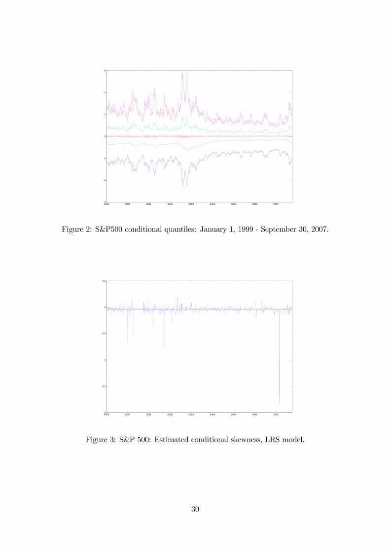
tistically significant at the usual significance level. Figure 2 displays plots of the

five individual quantiles for the time period under consideration.

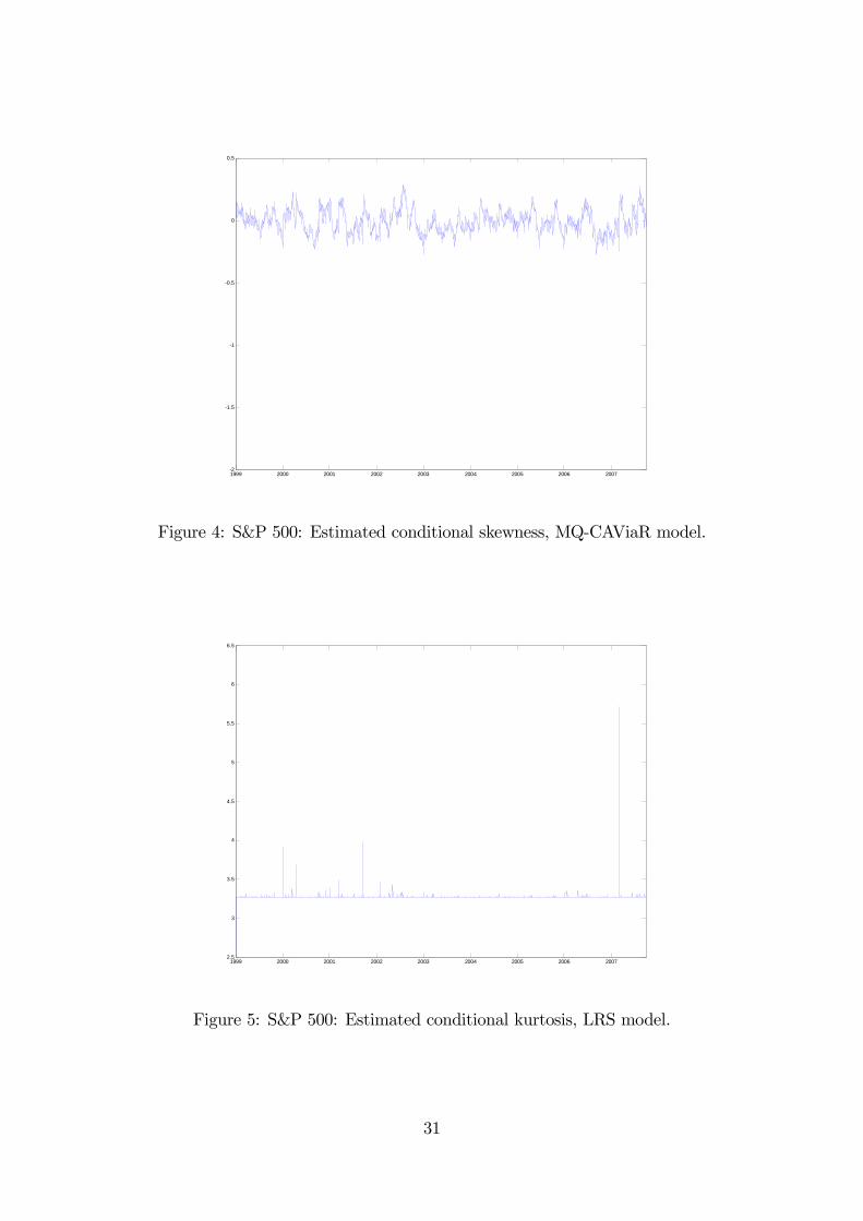
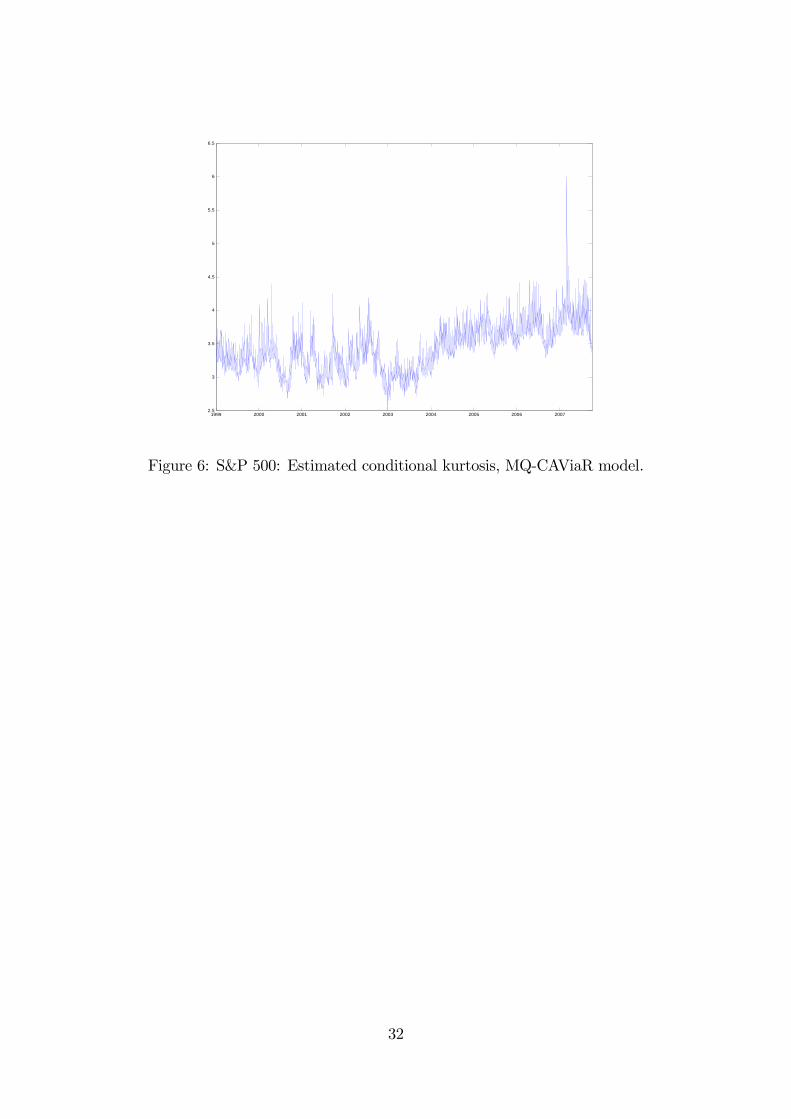
Next, we use the estimates of the individual quantiles q∗0.025,t, ..., q∗0.975,t to calcu-

late the robust skewness and kurtosis measures CSK2 and CKR4. The resulting

time-series plots are shown in Figures 4 and 6, respectively.

We observe that the LRS model estimates of both skewness and kurtosis do not

vary much and are dwarfed by those for the end of February 2007. The market was

doing well until February 27, when the S&P 500 index dropped by 3.5%, as the

market worried about global economic growth. (The sub-prime mortgage fiasco

was still not yet public knowledge.) Interestingly, this is not a particularly large

negative return (there are larger negative returns in our sample between 2000 and

2001), but this one occurred in a period of relatively low volatility.

Our more robust MQ-CAViaR measures show more plausible variability and

confirm that the February 2007 market correction was indeed a case of large neg-

ative conditional skewness and high conditional kurtosis. This episode appears

to be substantially affecting the LRS model estimates for the entire sample, rais-

ing doubts about the reliability of LRS estimates in general, consistent with the

findings of Sakata and White (1998).

13

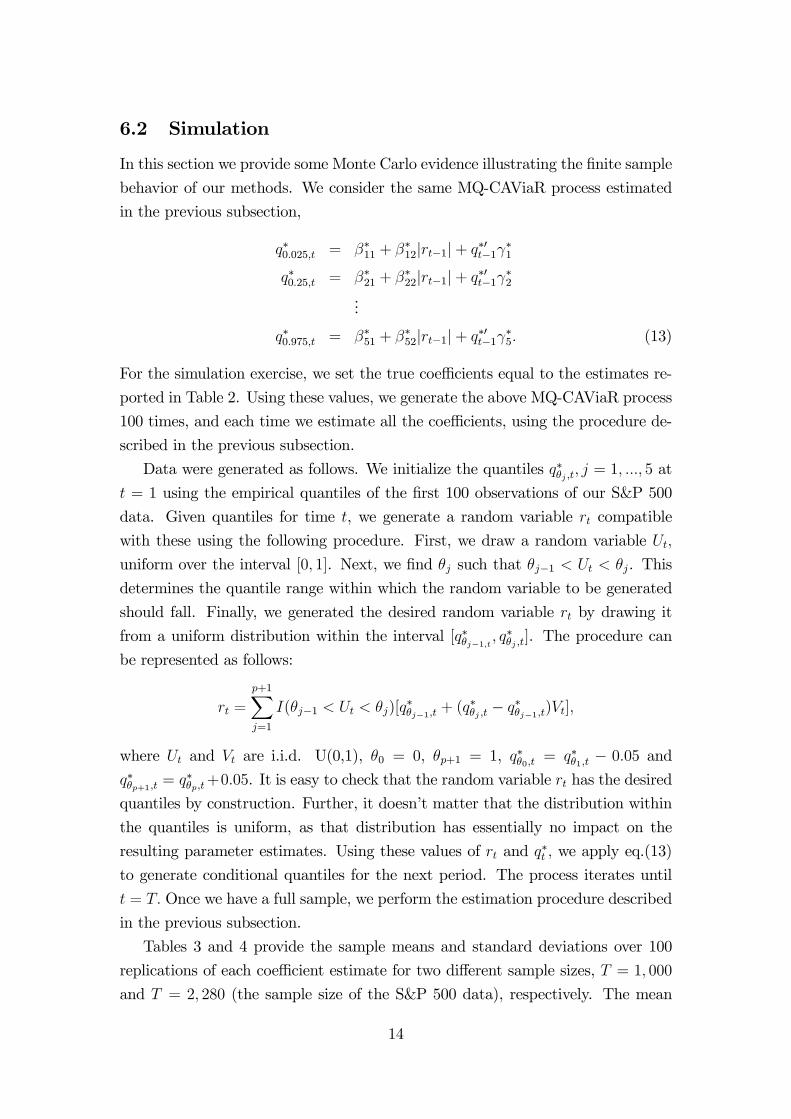
6.2 Simulation

In this section we provide some Monte Carlo evidence illustrating the finite sample

behavior of our methods. We consider the same MQ-CAViaR process estimated

in the previous subsection,

q∗0.025,t = β∗11 + β∗12|rt−1|+ q∗0t−1γ∗1

q∗0.25,t = β∗21 + β∗22|rt−1|+ q∗0t−1γ∗2

...

q∗0.975,t = β∗51 + β∗52|rt−1|+ q∗0t−1γ∗5. (13)

For the simulation exercise, we set the true coefficients equal to the estimates re-

ported in Table 2. Using these values, we generate the above MQ-CAViaR process

100 times, and each time we estimate all the coefficients, using the procedure de-

scribed in the previous subsection.

Data were generated as follows. We initialize the quantiles q∗θj ,t, j = 1, ..., 5 at

t = 1 using the empirical quantiles of the first 100 observations of our S&P 500

data. Given quantiles for time t, we generate a random variable rt compatible

with these using the following procedure. First, we draw a random variable Ut,

uniform over the interval [0, 1]. Next, we find θj such that θj−1 < Ut < θj. This

determines the quantile range within which the random variable to be generated

should fall. Finally, we generated the desired random variable rt by drawing it

from a uniform distribution within the interval [q∗θj−1,t , q∗θj ,t]. The procedure can

be represented as follows:

rt =

p+1Xj=1

I(θj−1 < Ut < θj)[q∗θj−1,t + (q

∗θj ,t− q∗θj−1,t)Vt],

where Ut and Vt are i.i.d. U(0,1), θ0 = 0, θp+1 = 1, q∗θ0,t = q∗θ1,t − 0.05 andq∗θp+1,t = q∗θp,t+0.05. It is easy to check that the random variable rt has the desired

quantiles by construction. Further, it doesn’t matter that the distribution within

the quantiles is uniform, as that distribution has essentially no impact on the

resulting parameter estimates. Using these values of rt and q∗t , we apply eq.(13)

to generate conditional quantiles for the next period. The process iterates until

t = T. Once we have a full sample, we perform the estimation procedure described

in the previous subsection.

Tables 3 and 4 provide the sample means and standard deviations over 100

replications of each coefficient estimate for two different sample sizes, T = 1, 000

and T = 2, 280 (the sample size of the S&P 500 data), respectively. The mean

14

estimates are fairly close to the values of Table 2, showing that the available sample

sizes are sufficient to recover the true DGP parameters. (To obtain standard error

estimates for the means, divide the reported standard deviations by 10.)

A potentially interesting experiment that one might consider is to generate data

from the LRS process and see how the MQ-CAViaR model performs in revealing

underlying patterns of conditional skewness and kurtosis. Nevertheless, we leave

this aside here, as the LRS model depends on four distributional shape parameters,

but we require five variation-free quantiles for the present exercise. As noted

in Section 2, the MQ-CAViaR model will generally not satisfy the identification

condition in such circumstances.

7 Conclusion

In this paper, we generalize Engle and Manganelli’s (2004) single-quantile CAViaR

process to its multi-quantile version. This allows for (i) joint modeling of multiple

quantiles; (ii) dynamic interactions between quantiles; and (iii) the use of exoge-

nous variables. We apply our MQ-CAViaR process to define conditional versions of

existing unconditional quantile-based measures of skewness and kurtosis. Because

of their use of quantiles, these measures may be much less sensitive than standard

moment-based methods to the adverse impact of outliers that regularly appear in

financial market data. An empirical analysis of the S&P 500 index demonstrates

the use and utility of our new methods.

References

[1] Andrews, D.W.K. (1988). Laws of large numbers for dependent non-

identically distributed random variables. Econometric Theory 4, 458-467.

[2] Bartle, R. (1966). The Elements of Integration. New York: Wiley.

[3] Bowley, A.L. (1920). Elements of Statistics. New York: Charles Scribner’s

Sons.

[4] Crow, E.L. and Siddiqui, M.M. (1967), Robust estimation of location. Journal

of the American Statistical Association 62, 353-389.

[5] Engle, R.F. and Manganelli, S. (2004). CAViaR: Conditional autoregressive

value at risk by regression quantiles. Journal of Business & Economic Statis-

tics 22, 367-381.

15

[6] Harvey, C.R. and Siddique, A. (2000). Conditional skewness in asset pricing

tests. Journal of Finance LV, 1263-1295.

[7] Huber, P.J. (1967). The behavior of maximum likelihood estimates under non-

standard conditions. Proceedings of the Fifth Berkeley Symposium on Math-

ematical Statistics and Probability, 221—233.

[8] Hwang, S. and Satchell, S.E. (1999). Modelling emerging market risk premia

using higher moments. International Journal of Finance and Economics 4,

271-296.

[9] Kim, T.-H. and White, H. (2003). Estimation, inference, and specification

testing for possibly misspecified quantile regression. In T. Fomby and C. Hill,

eds., Maximum Likelihood Estimation of Misspecified Models: Twenty Years

Later. New York: Elsevier, pp. 107-132.

[10] Kim, T.-H. and White, H. (2004). On more robust estimation of skewness

and kurtosis. Finance Research Letters 1, 56-73.

[11] Koenker, R. and Bassett, G. (1978). Regression quantiles. Econometrica 46,

33—50.

[12] Komunjer, I. (2005). Quasi-maximum likelihood estimation for conditional

quantiles. Journal of Econometrics 128, 127-164.

[13] Komunjer, I. and Vuong, Q. (2006). Efficient conditional quantile estima-

tion: the time series case. University of California, San Diego Department of

Economics Discussion Paper 2006-10, .

[14] Komunjer, I. and Vuong, Q. (2007a). Semiparametric efficiency bound and

M-estimation in time-series models for conditional quantiles. University of

California, San Diego Department of Economics Discussion Paper

[15] Komunjer, I. and Vuong, Q. (2007b). Efficient estimation in dynamic con-

ditional quantile models. University of California, San Diego Department of

Economics Discussion Paper.

[16] Leon, A., G. Rubio and G. Serna (2004), Autoregressive Conditional Volatil-

ity, Skewness and Kurtosis, WP-AD 2004-13, Instituto Valenciano de Inves-

tigaciones Economicas.

16

[17] Moors, J.J.A. (1988), A quantile alternative for kurtosis. The Statistician 37,

25-32.

[18] Otsu, T. (2003). Empirical likelihood for quantile regression. University of

Wisconsin, Madison Department of Economics Discussion Paper.

[19] Powell, J. (1984). Least absolute deviations estimators for the censored re-

gression model. Journal of Econometrics 25, 303-325.

[20] Newey, W.K. and Powell, J.L. (1990). Efficient estimation of linear and type

I censored regression models under conditional quantile restrictions. Econo-

metric Theory 6, 295-317.

[21] Sakata, S. andWhite, H. (1998). High breakdown point conditional dispersion

estimation with application to S&P 500 daily returns volatility. Econometrica

66, 529-568.

[22] Stinchcombe, M. and White, H. (1998). Consistent specification testing with

nuisance parameters present only under the alternative. Econometric Theory

14, 295-324.

[23] Weiss, A. (1991). Estimating nonlinear dynamic models using least absolute

error estimation. Econometric Theory 7, 46-68.

[24] White, H. (1994). Estimation, Inference and Specification Analysis. New

York: Cambridge University Press.

[25] White, H. (2001). Asymptotic Theory for Econometricians. San Diego: Aca-

demic Press.

[26] White, H. (2006). Approximate nonlinear forecasting methods. In G. Elliott,

C.W.J. Granger, and A. Timmermann, eds., Handbook of Economics Fore-

casting. New York: Elsevier, pp. 460-512

Mathematical Appendix

Proof of Theorem 1: We verify the conditions of corollary 5.11 of White (1994),which delivers αT → α∗, where

αT ≡ argmaxα∈

T−1TXt=1

ϕt(Yt, qt(·, α)),

17

and ϕt(Yt, qt(·, α)) ≡ −Pp

j=1 ρθj(Yt − qj,t(·, α)). Assumption 1 ensures White’sAssumption 2.1. Assumption 3(i) ensures White’s Assumption 5.1. Our choice of

ρθj satisfies White’s Assumption 5.4. To verify White’s Assumption 3.1, it suffices

that ϕt(Yt, qt(·, α)) is dominated on A by an integrable function (ensuring White’sAssumption 3.1(a,b)) and that for each α in A, ϕt(Yt, qt(·, α)) is stationaryand ergodic (ensuring White’s Assumption 3.1(c), the strong uniform law of large

numbers (ULLN)). Stationarity and ergodicity is ensured by Assumptions 1 and

3(i). To show domination, we write

|ϕt(Yt, qt(·, α))| ≤pX

j=1

|ρθj(Yt − qj,t(·, α))|

=

pXj=1

|(Yt − qj,t(·, α))(θj − 1[Yt−qj,t(·,α)≤0])|

≤ 2

pXj=1

|Yt|+ |qj,t(·, α)|

≤ 2p(|Yt|+ |D0,t|),

so that

supα∈

|ϕt(Yt, qt(·, α))| ≤ 2p(|Yt|+ |D0,t|).

Thus, 2p(|Yt| + |D0,t|) dominates |ϕt(Yt, qt(·, α))| and has finite expectation byAssumption 5(i,ii).

It remains to verify White’s Assumption 3.2; here this is the condition that

α∗ is the unique maximizer of E(ϕt(Yt, qt(·, α)). Given Assumptions 2(ii.b) and4(i), it follows by argument directly parallel to that in the proof of White (1994,

corollary 5.11) that for all α ∈ A,

E(ϕt(Yt, qt(·, α)) ≤ E(ϕt(Yt, qt(·, α∗)).

Thus, it suffices to show that the above inequality is strict for α 6= α∗. Letting

∆(α) ≡Pp

j=1E(∆j,t(α)) with ∆j,t(α) ≡ ρθj(Yt− qj,t(·, α))− ρθj(Yt− qj,t(·, α∗)), itsuffices to show that for each > 0, ∆(α) > 0 for all α ∈ A such that ||α−α∗|| > .

Pick > 0 and α ∈ A such that ||α − α∗|| > . With δj,t(α, α∗) ≡ qt(θj, α) −

qt(θj, α∗), by Assumption 4(i.b), there exist J ⊆ 1, ..., p and δ > 0 such that

P [∪j∈J|δj,t(α, α∗)| > δ ] > 0. For this δ and all j, some algebra and Assumption

18

2(ii.a) ensure that

E(∆j,t(α)) = E[

Z δj,t(α,α∗)

0

(δj,t(α, α∗)− s) fj,t(s)ds]

≥ E[1

2δ21[|δj,t(α,α∗)|>δ ] +

1

2δj,t(α, α

∗)21[|δj,t(α,α∗)|≤δ ])]

≥ 1

2δ2E[1[|δj,t(α,α∗)|>δ ]].

The first inequality above comes from the fact that Assumption 2(ii.a) implies

that for any δ > 0 sufficiently small, we have fj,t(s) > δ for |s| < δ . Thus,

∆(α) ≡pX

j=1

E(∆j,t(α)) ≥1

2δ2

pXj=1

E[1[|δj,t(α,α∗)|>δ ]]

=1

2δ2

pXj=1

P [|δj,t(α, α∗)| > δ ] ≥ 12δ2Xj∈J

P [|δj,t(α, α∗)| > δ ]

≥ 1

2δ2P [∪j∈J|δj,t(α, α∗)| > δ ]

> 0,

where the final inequality follows from Assumption 4(i.b). As > 0 and α are

arbitrary, the result follows.

Proof of Theorem 2: As outlined in the text, we first prove

T−1/2TXt=1

pXj=1

∇qj,t(·, αT ) ψθj(Yt − qj,t(·, αT )) = op(1). (14)

The existence of ∇qj,t is ensured by Assumption 3(ii). Let ei be the × 1 unitvector with ith element equal to one and the rest zero, and let

Gi(c) ≡ T−1/2TXt=1

pXj=1

ρθj(Yt − qj,t(·, αT + cei)),

for any real number c. Then by the definition of αT , Gi(c) is minimized at c = 0.

Let Hi(c) be the derivative of Gi(c) with respect to c from the right. Then

Hi(c) = −T−1/2TXt=1

pXj=1

∇iqj,t(·, αT + cei) ψθj(Yt − qj,t(·, αT + cei)),

where ∇iqj,t(·, αT +cei) is the ith element of ∇qj,t(·, αT +cei). Using the facts that

(i) Hi(c) is non-decreasing in c and (ii) for any > 0, Hi(− ) ≤ 0 and Hi( ) ≥ 0,

19

we have

|Hi(0)| ≤ Hi( )−Hi(− )

≤ T−1/2TXt=1

pXj=1

|∇iqj,t(·, αT )|1[Yt−qj,t(·,αT )=0]

≤ T−1/2 max1≤t≤T

D1,t

TXt=1

pXj=1

1[Yt−qj,t(·,αT )=0],

where the last inequality follows by the domination condition imposed in Assump-

tion 5(iii.a). Because D1,t is stationary, T−1/2max1≤t≤T D1,t = op(1). The second

term is bounded in probability:PT

t=1

Ppj=1 1[Yt−qj,t(·,αT )=0] = Op(1) given Assump-

tion 2(i,ii.a) (see Koenker and Bassett, 1978, for details). Since Hi(0) is the ith

element of T−1/2PT

t=1

Ppj=1∇qj,t(·, αT ) ψθj

(Yt − qj,t(·, αT )), the claim in (14) is

proved.

Next, for each α ∈ A, Assumptions 3(ii) and 5(iii.a) ensure the existence andfiniteness of the × 1 vector

λ(α) ≡pX

j=1

E[∇qj,t(·, α) ψθj(Yt − qj,t(·, α))]

=

pXj=1

E[∇qj,t(·, α)Z 0

δj,t(α,α∗)

fj,t(s)ds],

where δj,t(α, α∗) ≡ qj,t(·, α) − qj,t(·, α∗) and fj,t(s) = (d/ds)Ft(s + qj,t(·, α∗)) rep-resents the conditional density of εj,t ≡ Yt − qj,t(·, α∗) with respect to Lebesguemeasure. The differentiability and domination conditions provided by Assump-

tions 3(iii) and 5(iv.a) ensure (e.g., by Bartle, corollary 5.9??) the continuous

differentiability of λ on A, with

∇λ(α) =pX

j=1

E[∇∇0qj,t(·, α)Z 0

δj,t(α,α∗)

fj,t(s)ds].

Since α∗ is interior to A by Assumption 4(ii), the mean value theorem applies to

each element of λ to yield

λ(α) = λ(α∗) +Q0(α− α∗), (15)

for α in a convex compact neighborhood of α∗,where Q0 is an × matrix with

(1 × ) rows Qi(α(i)) = ∇0λi(α(i)), where α(i) is a mean value (different for eachi) lying on the segment connecting α and α∗, i = 1, ..., . The chain rule and an

application of the Leibniz rule toR 0δj,t(α,α∗)

fj,t(s)ds then give

Qi(α) = Ai(α)−Bi(α),

20

where

Ai(α) ≡pX

j=1

E[∇i∇0qj,t(·, α)Z 0

δj,t(α,α∗)fj,t(s)ds]

Bi(α) ≡pX

j=1

E[fj,t(δj,t(α, α∗))∇iqj,t(·, α)∇0qj,t(·, α)].

Assumption 2(iii) and the other domination conditions (those of Assumption 5)

then ensure that

Ai(α(i)) = O(||α− α∗||)Bi(α(i)) = Q∗i +O(||α− α∗||),

where Q∗i ≡Pp

j=1E[fj,t(0)∇iqj,t(·, α∗)∇0qj,t(·, α∗)]. Letting Q∗ ≡Pp

j=1E[fj,t(0)

× ∇qj,t(·, α∗)∇0qj,t(·, α∗)], we obtain

Q0 = −Q∗ +O(||α− α∗||). (16)

Next, we have that λ(α∗) = 0. To show this, we write

λ(α∗) =

pXj=1

E[∇qj,t(·, α∗) ψθj(Yt − qj,t(·, α∗))]

=

pXj=1

E(E[∇qj,t(·, α∗) ψθj(Yt − qj,t(·, α∗))|Ft−1])

=

pXj=1

E(∇qj,t(·, α∗) E[ψθj(Yt − qj,t(·, α∗))|Ft−1])

=

pXj=1

E(∇qj,t(·, α∗) E[ψθj(εj,t)|Ft−1])

= 0,

as E[ψθj(εj,t)|Ft−1] = θj − E[1[Yt≤q∗j,t]|Ft−1] = 0, by definition of q∗j,t, j = 1, ..., p

(see eq. (2)). Combining λ(α∗) = 0 with eqs. (15) and (16), we obtain

λ(α) = −Q∗(α− α∗) +O(||α− α∗||2). (17)

The next step is to show that

T 1/2λ(α) +HT = op(1) (18)

where HT ≡ T−1/2PT

t=1 η∗t , with η∗t ≡ ηt(α

∗), ηt(α) ≡Pp

j=1∇qj,t(·, α) ψθj(Yt −qj,t(·, α)). Let ut(α, d) ≡ supτ :||τ−α||≤d ||ηt(τ) − ηt(α)||. By the results of Huber

21

(1967) and Weiss (1991), to prove (18) it suffices to show the following: (i) there

exist a > 0 and d0 > 0 such that ||λ(α)|| ≥ a||α−α∗|| for ||α−α∗|| ≤ d0; (ii) there

exist b > 0, d0 > 0, and d ≥ 0 such that E[ut(α, d)] ≤ bd for ||α− α∗|| + d ≤ d0;

and (iii) there exist c > 0, d0 > 0, and d ≥ 0 such that E[ut(α, d)2] ≤ cd for

||α− α∗||+ d ≤ d0.

The condition that Q∗ is positive-definite in Assumption 6(i) is sufficient for

(i). For (ii), we have that for given (small) d > 0

ut(α, d) ≤ supτ :||τ−α||≤d

pXj=1

||∇qj,t(·, τ)ψθj(Yt − qj,t(·, τ))−∇qj,t(·, α)ψθj(Yt − qj,t(·, α))||

≤pX

j=1

supτ :||τ−α||≤d

||ψθj(Yt − qj,t(·, τ))|| × sup

τ :||τ−α||≤d||∇qj,t(·, τ)−∇qj,t(·, α)||

+

pXj=1

supτ :||τ−α||≤d

||ψθj(Yt − qj,t(·, α))− ψθj

(Yt − qj,t(·, τ))|| × supτ :||τ−α||≤d

||∇qj,t(·, α)||

≤ pD2,td+D1,t

pXj=1

1[|Yt−qj,t(·,α)|<D2,td] (19)

using the following; (i) ||ψθj(Yt−qj,t(·, τ))|| ≤ 1, (ii) ||ψθj(Yt−qj,t(·, α))−ψθj(Yt−qj,t(·, τ))|| ≤ 1[|Yt−qj,t(·,α)|<|qj,t(·,τ)−qj,t(·,α)|], and (iii) the mean value theorem appliedto ∇qj,t(·, τ) and qj,t(·, α). Hence, we have

E[ut(α, d)] ≤ pC0d+ 2pC1f0d

for some constants C0 and C1 given Assumptions 2(iii.a), 5(iii.a), and 5(iv.a).

Hence, (ii) holds for b = pC0 + 2pC1f0 and d0 = 2d. The last condition (iii) can

be similarly verified by applying the cr−inequality to eq. (19) with d < 1 (so thatd2 < d) and using Assumptions 2(iii.a), 5(iii.b), and 5(iv.b). Thus, eq. (18) is

verified .

Combining eqs. (17) and (18) thus yields

Q∗T 1/2(αT − α∗) = T−1/2TXt=1

η∗t + op(1)

But η∗t ,Ft is a stationary ergodic martingale difference sequence (MDS). In par-ticular, η∗t is measurable−Ft, andE(η∗t |Ft−1) = E(

Ppj=1∇qj,t(·, α∗)ψθj(εj,t)|Ft−1) =Pp

j=1∇qj,t(·, α∗)E(ψθj(εj,t)|Ft−1) = 0, as E[ψθj(εj,t)|Ft−1] = 0 for all j = 1, ..., p.

Assumption 5(iii.b) ensures that V ∗ ≡ E(η∗tη∗0t ) is finite. The MDS central limit

theorem (e.g., theorem 5.24 of White, 2001) applies, provided V ∗ is positive defi-

nite (as ensured by Assumption 6(ii)) and that T−1PT

t=1 η∗tη∗0t = V ∗+op(1), which

22

is ensured by the ergodic theorem. The standard argument now gives

V ∗−1/2Q∗T 1/2(αT − α∗)d→ N(0, I),

which completes the proof.

Proof of Theorem 3: We have

VT − V ∗ = (T−1TXt=1

ηtη0t − T−1

TXt=1

η∗tη∗0t ) + (T

−1TXt=1

η∗tη∗0t −E[η∗tη

∗0t ]),

where ηt ≡Pp

j=1∇qj,tψj,t and η∗t ≡

Ppj=1∇q∗j,tψ∗j,t, with∇qj,t ≡ ∇qj,t(·, αT ), ψj,t ≡

ψθj(Yt − qj,t(·, αT )),∇q∗j,t ≡ ∇qj,t(·, α∗), and ψ∗j,t ≡ ψθj

(Yt − qj,t(·, α∗)). Assump-tions 1 and 2(i,ii) ensure that η∗tη∗0t is a stationary ergodic sequence. Assump-tions 3(i,ii), 4(i.a), and 5(iii) ensure that E[η∗tη

∗0t ] < ∞. It follows by the er-

godic theorem that T−1PT

t=1 η∗tη∗0t − E[η∗tη

∗0t ] = op(1). Thus, it suffices to prove

T−1PT

t=1 ηtη0t − T−1

PTt=1 η

∗tη∗0t = op(1).

The (h, i) element of T−1PT

t=1 ηtη0t − T−1

PTt=1 η

∗tη∗0t is

T−1TXt=1

pX

j=1

pXk=1

ψj,tψk,t∇hqj,t∇iqk,t − ψ∗j,tψ∗k,t∇hq

∗j,t∇iq

∗k,t.

Thus, it will suffice to show that for each (h, i) and (j, k) we have

T−1TXt=1

ψj,tψk,t∇hqj,t∇iqk,t − ψ∗j,tψ∗k,t∇hq

∗j,t∇iq

∗k,t = op(1).

By the triangle inequality,

|T−1TXt=1

ψj,tψk,t∇hqj,t∇iqk,t − ψ∗j,tψ∗k,t∇hq

∗j,t∇iq

∗k,t| ≤ AT +BT ,

where

AT = |T−1TXt=1

ψj,tψk,t∇hqj,t∇iqk,t − ψ∗j,tψ∗k,t∇hqj,t∇iqk,t|

BT = |T−1TXt=1

ψ∗j,tψ∗k,t∇hq

∗j,t∇iq

∗k,t − ψ∗j,tψ

∗k,t∇hqj,t∇iqk,t|.

We now show that AT = op(1) and BT = op(1), delivering the desired result.

For AT , the triangle inequality gives

AT ≤ A1T +A2T +A3T ,

23

where

A1T = T−1TXt=1

θj|1[εj,t≤0] − 1[εj,t≤0]||∇hqj,t∇iqk,t|

A2T = T−1TXt=1

θk|1[εk,t≤0] − 1[εk,t≤0]||∇hqj,t∇iqk,t|

A3T = T−1TXt=1

|1[εj,t≤0]1[εk,t≤0] − 1[εj,t≤0]1[εk,t≤0]||∇hqj,t∇iqk,t|.

Theorem 2, ensured by Assumptions 1− 6, implies that T 1/2||αT − α∗|| = Op(1).

This, together with Assumptions 2(iii,iv) and 5(iii.b), enables us to apply the

same techniques used in Kim and White (2003) to show A1T = op(1), A2T =

op(1), A3T = op(1), implying AT = op(1).

It remains to show BT = op(1). By the triangle inequality,

BT ≤ B1T +B2T ,

where

B1T = |T−1TXt=1

ψ∗j,tψ∗k,t∇hq

∗j,t∇iq

∗k,t − E[ψ∗j,tψ

∗k,t∇hq

∗j,t∇iq

∗k,t]|

B2T = |T−1TXt=1

ψ∗j,tψ∗k,t∇hqj,t∇iqk,t − E[ψ∗j,tψ

∗k,t∇hq

∗j,t∇iq

∗k,t]|.

Assumptions 1, 2(i,ii), 3(i,ii), 4(i.a), and 5(iii) ensure that the ergodic theorem

applies to ψ∗j,tψ∗k,t∇hq∗j,t∇iq

∗k,t, so B1T = op(1). Next, Assumptions 1, 3(i,ii), and

5(iii) ensure that the stationary ergodic ULLN applies to ψ∗j,tψ∗k,t∇hqj,t(·, α)∇iqk,t(·, α).This and the result of Theorem 1 (αT − α∗ = op(1)) ensure that B2T = op(1) by

e.g., White (1994, corollary 3.8), and the proof is complete.

Proof of Theorem 4: We begin by sketching the proof. We first define

QT ≡ (2cTT )−1TXt=1

pXj=1

1[−cT≤εj,t≤cT ]∇q∗j,t∇0q∗j,t,

and then we will show the following:

Q∗ −E(QT )p→ 0, (20)

E(QT )−QTp→ 0, (21)

QT − QTp→ 0. (22)

24

Combining the results above will deliver the desired outcome: QT −Q∗p→ 0.

For (20), one can show by applying the mean value theorem to Fj,t(cT ) −Fj,t(−cT ), where Fj,t(c) ≡

R1s≤cfj,t(s)ds, that

E(QT ) = T−1TXt=1

pXj=1

E[fj,t(ξj,T )∇q∗j,t∇0q∗j,t] =pX

j=1

E[fj,t(ξj,T )∇q∗j,t∇0q∗j,t],

where ξj,T is a mean value lying between −cT and cT , and the second equality

follows by stationarity. Therefore, the (h, i) element of |E(QT )−Q∗| satisfies

|pX

j=1

E©fj,t(ξj,T )− fj,t(0)∇hq

∗j,t∇iq

∗j,t

ª|

≤pX

j=1

E©|fj,t(ξj,T )− fj,t(0)||∇hq

∗j,t∇iq

∗j,t|ª

≤pX

j=1

L0E©|ξj,T ||∇hq

∗j,t∇iq

∗j,t|ª

≤ pL0cTE[D21,t],

which converges to zero as cT → 0. The second inequality follows by Assumption

2(iii.b), and the last inequality follows by Assumption 5(iii.b). Therefore, we have

the result in eq.(20).

To show (21), it suffices simply to apply a LLN for double arrays, e.g. theorem

2 in Andrews (1988).

Finally, for (22), we consider the (h, i) element of |QT −QT |, which is given by

| 1

2cTT

TXt=1

pXj=1

1[−cT≤εj,t≤cT ]∇hqj,t∇iqj,t −1

2cTT

TXt=1

pXj=1

1[−cT≤εj,t≤cT ]∇hq∗j,t∇iq

∗j,t|

=cTcT| 1

2cTT

TXt=1

pXj=1

(1[−cT≤εj,t≤cT ] − 1[−cT≤εj,t≤cT ])∇hqj,t∇iqj,t

+1

2cTT

TXt=1

pXj=1

1[−cT≤εj,t≤cT ](∇hqj,t −∇hq∗j,t)∇iqj,t

+1

2cTT

TXt=1

pXj=1

1[−cT≤εj,t≤cT ]∇hq∗j,t(∇iqj,t −∇iq

∗j,t)

+1

2cTT(1− cT

cT)

TXt=1

pXj=1

1[−cT≤εj,t≤cT ]∇hq∗j,t∇iq

∗j,t|

≤ cTcT[A1T +A2T +A3T + (1−

cTcT)A4T ],

25

where

A1T ≡ 1

2cTT

TXt=1

pXj=1

|1[−cT≤εj,t≤cT ] − 1[−cT≤εj,t≤cT ]| × |∇hqj,t∇iqj,t|

A2T ≡ 1

2cTT

TXt=1

pXj=1

1[−cT≤εj,t≤cT ]|∇hqj,t −∇hq∗j,t| × |∇iqj,t|

A3T ≡ 1

2cTT

TXt=1

pXj=1

1[−cT≤εj,t≤cT ]|∇hq∗j,t| × |∇iqj,t −∇iq

∗j,t|

A4T ≡ 1

2cTT

TXt=1

pXj=1

1[−cT≤εj,t≤cT ]|∇hq∗j,t∇iq

∗j,t|.

It will suffice to show that A1T = op(1), A2T = op(1), A3T = op(1), and A4T =

Op(1). Then, because cT/cTp→ 1, we obtain the desired result: QT −Q∗

p→ 0.

We first show A1T = op(1). It will suffice to show that for each j,

1

2cTT

TXt=1

|1[−cT≤εj,t≤cT ] − 1[−cT≤εj,t≤cT ]| × |∇hqj,t∇iqj,t| = op(1).

Let αT lie between αT and α∗, and put dj,t,T ≡ ||∇qj,t(·, αT )||×||αT−α∗||+|cT−cT |.Then

(2cTT )−1

TXt=1

|1[−cT≤εj,t≤cT ] − 1[−cT≤εj,t≤cT ]| × |∇hqj,t∇iqj,t| ≤ UT + VT ,

where

UT ≡ (2cTT )−1

TXt=1

1[|εj,t−cT |<dj,t,T ]|∇hqj,t∇iqj,t|

VT ≡ (2cTT )−1

TXt=1

1[|εj,t+cT |<dj,t,T ]|∇hqj,t∇iqj,t|.

It will suffice to show that UTp→ 0 and VT

p→ 0. Let η > 0 and let z be an arbitrary

positive number. Then, using reasoning similar to that of Kim and White (2003,

lemma 5), one can show that for any η > 0,

P (UT > η) ≤ P ((2cTT )−1

TXt=1

1[|εj,t−cT |<(||∇qt(θj ,α0)||+1)zcT ])|∇hqj,t∇iqj,t| > η)

≤ zf0ηT

TXt=1

E (||∇qt(θj, αT )||+ 1)|∇hqj,t∇iqj,t|

≤ zf0E|D31,t|+E|D2

1,t|/η,

26

where the second inequality is due to the Markov inequality and Assumption

2(iii.a), and the third is due to Assumption 5(iii.c). As z can be chosen arbitrarily

small and the remaining terms are finite by assumption, we have UTp→ 0. The

same argument is used to show VTp→ 0. Hence, A1T = op(1) is proved.

Next, we show A2T = op(1). For this, it suffices to show A2T,j ≡ 12cTT

PTt=1

1[−cT≤εj,t≤cT ]|∇hqj,t −∇hq∗j,t| × |∇iqj,t| = op(1) for each j. Note that

A2T,j ≤1

2cTT

TXt=1

|∇hqj,t −∇hq∗j,t| × |∇iqj,t|

≤ 1

2cTT

TXt=1

||∇2hqj,t(·, α)|| × ||αT − α∗|| × |∇iqj,t|

≤ 1

2cT||αT − α∗|| 1

T

TXt=1

D2,tD1,t

=1

2cTT 1/2T 1/2||αT − α∗|| 1

T

TXt=1

D2,tD1,t,

where α is between αT and α∗, and ∇2hqj,t(·, α) is the first derivative of ∇hqj,t

with respect to α, which is evaluated at α. The last expression above is op(1)

because (i) T 1/2||αT − α∗|| = Op(1) by Theorem 2, (ii) T−1PT

t=1D2,tD1,t = Op(1)

by the ergodic theorem and (iii) 1/(cTT 1/2) = op(1) by Assumption 7(iii). Hence,

A2T = op(1). The other claims A3T = op(1) and A4T = Op(1) can be analogously

and more easily proven. Hence, they are omitted. Therefore, we finally have

QT − QTp→ 0, which, together with (20) and (21), implies that QT − Q∗

p→ 0.

The proof is complete.

27

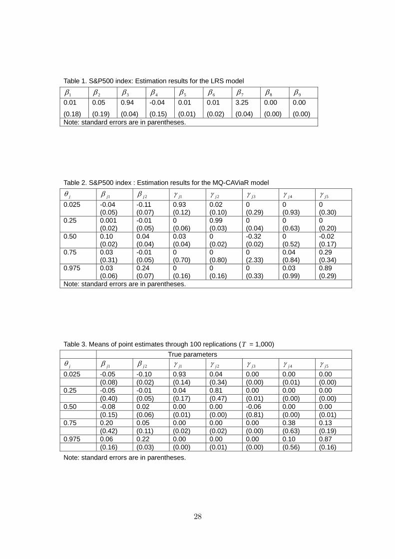
Table 1. S&P500 index: Estimation results for the LRS model

1β 2β 3β 4β 5β 6β 7β 8β 9β 0.01 0.05 0.94 -0.04 0.01 0.01 3.25 0.00 0.00

(0.18) (0.19) (0.04) (0.15) (0.01) (0.02) (0.04) (0.00) (0.00) Note: standard errors are in parentheses.

Table 2. S&P500 index : Estimation results for the MQ-CAViaR model

jθ 1jβ 2jβ 1jγ 2jγ 3jγ 4jγ 5jγ

0.025 -0.04 (0.05)

-0.11 (0.07)

0.93 (0.12)

0.02 (0.10)

0 (0.29)

0 (0.93)

0 (0.30)

0.25 0.001 (0.02)

-0.01 (0.05)

0 (0.06)

0.99 (0.03)

0 (0.04)

0 (0.63)

0 (0.20)

0.50 0.10 (0.02)

0.04 (0.04)

0.03 (0.04)

0 (0.02)

-0.32 (0.02)

0 (0.52)

-0.02 (0.17)

0.75 0.03 (0.31)

-0.01 (0.05)

0 (0.70)

0 (0.80)

0 (2.33)

0.04 (0.84)

0.29 (0.34)

0.975 0.03 (0.06)

0.24 (0.07)

0 (0.16)

0 (0.16)

0 (0.33)

0.03 (0.99)

0.89 (0.29)

Note: standard errors are in parentheses.

Table 3. Means of point estimates through 100 replications (T = 1,000) True parameters

jθ 1jβ 2jβ 1jγ 2jγ 3jγ 4jγ 5jγ

0.025 -0.05 -0.10 0.93 0.04 0.00 0.00 0.00 (0.08) (0.02) (0.14) (0.34) (0.00) (0.01) (0.00) 0.25 -0.05 -0.01 0.04 0.81 0.00 0.00 0.00 (0.40) (0.05) (0.17) (0.47) (0.01) (0.00) (0.00) 0.50 -0.08 0.02 0.00 0.00 -0.06 0.00 0.00 (0.15) (0.06) (0.01) (0.00) (0.81) (0.00) (0.01) 0.75 0.20 0.05 0.00 0.00 0.00 0.38 0.13 (0.42) (0.11) (0.02) (0.02) (0.00) (0.63) (0.19) 0.975 0.06 0.22 0.00 0.00 0.00 0.10 0.87 (0.16) (0.03) (0.00) (0.01) (0.00) (0.56) (0.16) Note: standard errors are in parentheses.

28

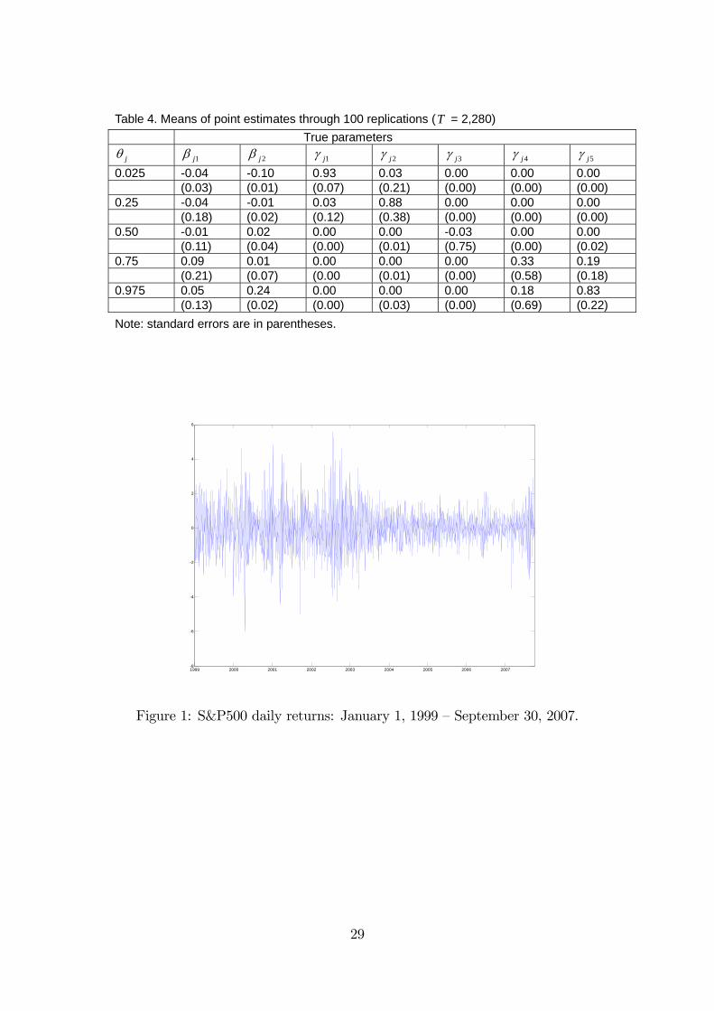
Table 4. Means of point estimates through 100 replications (T = 2,280) True parameters

jθ 1jβ 2jβ 1jγ 2jγ 3jγ 4jγ 5jγ

0.025 -0.04 -0.10 0.93 0.03 0.00 0.00 0.00 (0.03) (0.01) (0.07) (0.21) (0.00) (0.00) (0.00) 0.25 -0.04 -0.01 0.03 0.88 0.00 0.00 0.00 (0.18) (0.02) (0.12) (0.38) (0.00) (0.00) (0.00) 0.50 -0.01 0.02 0.00 0.00 -0.03 0.00 0.00 (0.11) (0.04) (0.00) (0.01) (0.75) (0.00) (0.02) 0.75 0.09 0.01 0.00 0.00 0.00 0.33 0.19 (0.21) (0.07) (0.00 (0.01) (0.00) (0.58) (0.18) 0.975 0.05 0.24 0.00 0.00 0.00 0.18 0.83 (0.13) (0.02) (0.00) (0.03) (0.00) (0.69) (0.22) Note: standard errors are in parentheses.

1999 2000 2001 2002 2003 2004 2005 2006 2007-8

-6

-4

-2

0

2

4

6

Figure 1: S&P500 daily returns: January 1, 1999 — September 30, 2007.

29

1999 2000 2001 2002 2003 2004 2005 2006 2007-6

-4

-2

0

2

4

6

Figure 2: S&P500 conditional quantiles: January 1, 1999 - September 30, 2007.

1999 2000 2001 2002 2003 2004 2005 2006 2007-2

-1.5

-1

-0.5

0

0.5

Figure 3: S&P 500: Estimated conditional skewness, LRS model.

30

1999 2000 2001 2002 2003 2004 2005 2006 2007-2

-1.5

-1

-0.5

0

0.5

Figure 4: S&P 500: Estimated conditional skewness, MQ-CAViaR model.

1999 2000 2001 2002 2003 2004 2005 2006 20072.5

3

3.5

4

4.5

5

5.5

6

6.5

Figure 5: S&P 500: Estimated conditional kurtosis, LRS model.

31

1999 2000 2001 2002 2003 2004 2005 2006 20072.5

3

3.5

4

4.5

5

5.5

6

6.5

Figure 6: S&P 500: Estimated conditional kurtosis, MQ-CAViaR model.

32