Embed Size (px)
Citation preview

Modeling and Solving inAnswer Set Programming
Martin Gebser Roland Kaminski Benjamin Kaufmann
Torsten Schaub
University of Potsdam
Torsten Schaub et al. (KRR@UP) Modeling and Solving in ASP 1 / 226

Outline
1 Motivation
2 Introduction
3 Basic modeling
4 (Language extensions)
5 Solving
6 Advanced modeling
7 Systems
8 Summary
Bibliography
Torsten Schaub et al. (KRR@UP) Modeling and Solving in ASP 2 / 226

Bias
Focus
Answer Set Programming as Boolean Constraint Satisfaction Problem
Answer Set Solving as a Boolean Constraint Solving
Answer Set Systems at http://potassco.sourceforge.net
Further resources
http://potassco.sourceforge.net/teaching.html
Torsten Schaub et al. (KRR@UP) Modeling and Solving in ASP 3 / 226

Motivation: Overview
1 Motivation
2 Nutshell
3 Shifting paradigms
4 Rooting ASP
5 Problem solving
6 Use
Torsten Schaub et al. (KRR@UP) Modeling and Solving in ASP 4 / 226

Motivation
Motivation: Overview
1 Motivation
2 Nutshell
3 Shifting paradigms
4 Rooting ASP
5 Problem solving
6 Use
Torsten Schaub et al. (KRR@UP) Modeling and Solving in ASP 5 / 226

Motivation
Informatics
“What is the problem?” versus “How to solve the problem?”
Problem
Computer
Solution
Output?
-
6
Torsten Schaub et al. (KRR@UP) Modeling and Solving in ASP 6 / 226

Motivation
Informatics
“What is the problem?” versus “How to solve the problem?”
Problem
Computer
Solution
Output?
-
6
Torsten Schaub et al. (KRR@UP) Modeling and Solving in ASP 6 / 226

Motivation
Traditional programming
“What is the problem?” versus “How to solve the problem?”
Problem
Computer
Solution
Output?
-
6
Torsten Schaub et al. (KRR@UP) Modeling and Solving in ASP 6 / 226

Motivation
Traditional programming
“What is the problem?” versus “How to solve the problem?”
Problem
Program
Solution
Output?
-
6
Programming Interpreting
Executing
Torsten Schaub et al. (KRR@UP) Modeling and Solving in ASP 6 / 226

Motivation
Declarative problem solving
“What is the problem?” versus “How to solve the problem?”
Problem
Computer
Solution
Output?
-
6
Interpreting
Torsten Schaub et al. (KRR@UP) Modeling and Solving in ASP 6 / 226

Motivation
Declarative problem solving
“What is the problem?” versus “How to solve the problem?”
Problem
Representation
Solution
Output?
-
6
Modeling Interpreting
Solving
Torsten Schaub et al. (KRR@UP) Modeling and Solving in ASP 6 / 226

Motivation
Declarative problem solving
“What is the problem?” versus “How to solve the problem?”
Problem
Representation
Solution
Output?
-
6
Modeling Interpreting
Solving
Torsten Schaub et al. (KRR@UP) Modeling and Solving in ASP 6 / 226

Nutshell
Motivation: Overview
1 Motivation
2 Nutshell
3 Shifting paradigms
4 Rooting ASP
5 Problem solving
6 Use
Torsten Schaub et al. (KRR@UP) Modeling and Solving in ASP 7 / 226

Nutshell
Answer Set Programmingin a Nutshell
ASP is an approach to declarative problem solving, combininga rich yet simple modeling languagewith high-performance solving capacities
ASP has its roots in(logic-based) knowledge representation and (nonmonotonic) reasoning(deductive) databasesconstraint solving (in particular, SATisfiability testing)logic programming (with negation)
ASP allows for solving all search problems in NP (and NPNP)in a uniform way
ASP is versatile as reflected by the ASP solver clasp, winningfirst places at ASP’07/09/11, CASC’11, MISC’11, PB’09/11,and SAT’09/11
ASP embraces many emerging application areas
Torsten Schaub et al. (KRR@UP) Modeling and Solving in ASP 8 / 226

Nutshell
Answer Set Programmingin a Peanutshell
ASP is an approach to declarative problem solving, combining
a rich yet simple modeling languagewith high-performance solving capacities
tailored to Knowledge Representation and Reasoning
Torsten Schaub et al. (KRR@UP) Modeling and Solving in ASP 9 / 226

Nutshell
Answer Set Programmingin a Peanutshell
ASP is an approach to declarative problem solving, combining
a rich yet simple modeling languagewith high-performance solving capacities
tailored to Knowledge Representation and Reasoning
ASP = KR+DB+SAT+LP
Torsten Schaub et al. (KRR@UP) Modeling and Solving in ASP 9 / 226

Shifting paradigms
Motivation: Overview
1 Motivation
2 Nutshell
3 Shifting paradigms
4 Rooting ASP
5 Problem solving
6 Use
Torsten Schaub et al. (KRR@UP) Modeling and Solving in ASP 10 / 226

Shifting paradigms
KR’s shift of paradigm
Theorem Proving based approach (eg. Prolog)
1 Provide a representation of the problem.2 A solution is given by a derivation of a query.
Model Generation based approach (eg. SATisfiability testing)
1 Provide a representation of the problem.2 A solution is given by a model of the representation.
Automated planning, Kautz and Selman (ECAI’92)
Represent planning problems as propositional theories so thatmodels not proofs describe solutions
Torsten Schaub et al. (KRR@UP) Modeling and Solving in ASP 11 / 226

Shifting paradigms
Model Generation based Problem Solving
Representation Solutionconstraint satisfaction problem assignment
propositional horn theories smallest model
propositional theories models
SAT
propositional theories minimal modelspropositional theories stable models
propositional programs minimal modelspropositional programs supported modelspropositional programs stable models
first-order theories modelsfirst-order theories minimal modelsfirst-order theories stable modelsfirst-order theories Herbrand models
auto-epistemic theories expansionsdefault theories extensions
......
Torsten Schaub et al. (KRR@UP) Modeling and Solving in ASP 12 / 226

Shifting paradigms
Model Generation based Problem Solving
Representation Solutionconstraint satisfaction problem assignment
propositional horn theories smallest model
propositional theories models SATpropositional theories minimal modelspropositional theories stable models
propositional programs minimal modelspropositional programs supported modelspropositional programs stable models
first-order theories modelsfirst-order theories minimal modelsfirst-order theories stable modelsfirst-order theories Herbrand models
auto-epistemic theories expansionsdefault theories extensions
......
Torsten Schaub et al. (KRR@UP) Modeling and Solving in ASP 12 / 226

Shifting paradigms
LP-style playing with blocks
Prolog program
on(a,b).
on(b,c).
above(X,Y) :- on(X,Y).
above(X,Y) :- on(X,Z), above(Z,Y).
Prolog queries
?- above(a,c).
true.
?- above(c,a).
no.
Torsten Schaub et al. (KRR@UP) Modeling and Solving in ASP 13 / 226

Shifting paradigms
LP-style playing with blocks
Prolog program
on(a,b).
on(b,c).
above(X,Y) :- on(X,Y).
above(X,Y) :- on(X,Z), above(Z,Y).
Prolog queries
?- above(a,c).
true.
?- above(c,a).
no.
Torsten Schaub et al. (KRR@UP) Modeling and Solving in ASP 13 / 226

Shifting paradigms
LP-style playing with blocks
Another Prolog program
on(a,b).
on(b,c).
above(X,Y) :- above(X,Z), on(Z,Y).
above(X,Y) :- on(X,Y).
Prolog queries
?- above(a,c).
Fatal Error: local stack overflow.
Torsten Schaub et al. (KRR@UP) Modeling and Solving in ASP 14 / 226

Shifting paradigms
LP-style playing with blocks
Another Prolog program
on(a,b).
on(b,c).
above(X,Y) :- above(X,Z), on(Z,Y).
above(X,Y) :- on(X,Y).
Prolog queries
?- above(a,c).
Fatal Error: local stack overflow.
Torsten Schaub et al. (KRR@UP) Modeling and Solving in ASP 14 / 226

Shifting paradigms
SAT-style playing with blocks
Formula
on(a, b)∧ on(b, c)∧ (on(X ,Y )→ above(X ,Y ))∧ (on(X ,Z ) ∧ above(Z ,Y )→ above(X ,Y ))
Herbrand model
{on(b, b), on(a, b), on(b, c), on(a, c),above(b, b), above(c , b), above(a, b),above(b, c), above(c , c), above(a, c) }
Torsten Schaub et al. (KRR@UP) Modeling and Solving in ASP 15 / 226

Shifting paradigms
SAT-style playing with blocks
Formula
on(a, b)∧ on(b, c)∧ (on(X ,Y )→ above(X ,Y ))∧ (on(X ,Z ) ∧ above(Z ,Y )→ above(X ,Y ))
Herbrand model (among 426!)
{on(b, b), on(a, b), on(b, c), on(a, c),above(b, b), above(c , b), above(a, b),above(b, c), above(c , c), above(a, c) }
Torsten Schaub et al. (KRR@UP) Modeling and Solving in ASP 15 / 226

Rooting ASP
Motivation: Overview
1 Motivation
2 Nutshell
3 Shifting paradigms
4 Rooting ASP
5 Problem solving
6 Use
Torsten Schaub et al. (KRR@UP) Modeling and Solving in ASP 16 / 226

Rooting ASP
KR’s shift of paradigm
Theorem Proving based approach (eg. Prolog)
1 Provide a representation of the problem.2 A solution is given by a derivation of a query.
Model Generation based approach (eg. SATisfiability testing)
1 Provide a representation of the problem.2 A solution is given by a model of the representation.
Torsten Schaub et al. (KRR@UP) Modeling and Solving in ASP 17 / 226

Rooting ASP
KR’s shift of paradigm
Theorem Proving based approach (eg. Prolog)
1 Provide a representation of the problem.2 A solution is given by a derivation of a query.
Model Generation based approach (eg. SATisfiability testing)
1 Provide a representation of the problem.2 A solution is given by a model of the representation.
å Answer Set Programming (ASP)
Torsten Schaub et al. (KRR@UP) Modeling and Solving in ASP 17 / 226

Rooting ASP
Model Generation based Problem Solving
Representation Solutionconstraint satisfaction problem assignment
propositional horn theories smallest model
propositional theories modelspropositional theories minimal modelspropositional theories stable models
propositional programs minimal modelspropositional programs supported modelspropositional programs stable models
first-order theories modelsfirst-order theories minimal modelsfirst-order theories stable modelsfirst-order theories Herbrand models
auto-epistemic theories expansionsdefault theories extensions
......
Torsten Schaub et al. (KRR@UP) Modeling and Solving in ASP 18 / 226

Rooting ASP
Answer Set Programming at large
Representation Solutionconstraint satisfaction problem assignment
propositional horn theories smallest model
propositional theories modelspropositional theories minimal modelspropositional theories stable models
propositional programs minimal modelspropositional programs supported modelspropositional programs stable models
first-order theories modelsfirst-order theories minimal modelsfirst-order theories stable modelsfirst-order theories Herbrand models
auto-epistemic theories expansionsdefault theories extensions
......
Torsten Schaub et al. (KRR@UP) Modeling and Solving in ASP 18 / 226

Rooting ASP
Answer Set Programming commonly
Representation Solutionconstraint satisfaction problem assignment
propositional horn theories smallest model
propositional theories modelspropositional theories minimal modelspropositional theories stable models
propositional programs minimal modelspropositional programs supported modelspropositional programs stable models
first-order theories modelsfirst-order theories minimal modelsfirst-order theories stable modelsfirst-order theories Herbrand models
auto-epistemic theories expansionsdefault theories extensions
......
Torsten Schaub et al. (KRR@UP) Modeling and Solving in ASP 18 / 226

Rooting ASP
Answer Set Programming in practice
Representation Solutionconstraint satisfaction problem assignment
propositional horn theories smallest model
propositional theories modelspropositional theories minimal modelspropositional theories stable models
propositional programs minimal modelspropositional programs supported modelspropositional programs stable models
first-order theories modelsfirst-order theories minimal modelsfirst-order theories stable modelsfirst-order theories Herbrand models
auto-epistemic theories expansionsdefault theories extensions
first-order programs stable Herbrand models
Torsten Schaub et al. (KRR@UP) Modeling and Solving in ASP 18 / 226

Rooting ASP
ASP-style playing with blocks
Prolog program
on(a,b).
on(b,c).
above(X,Y) :- on(X,Y).
above(X,Y) :- on(X,Z), above(Z,Y).
Stable Herbrand model
{ on(a, b), on(b, c), above(b, c), above(a, b), above(a, c) }
Torsten Schaub et al. (KRR@UP) Modeling and Solving in ASP 19 / 226

Rooting ASP
ASP-style playing with blocks
Prolog program
on(a,b).
on(b,c).
above(X,Y) :- on(X,Y).
above(X,Y) :- on(X,Z), above(Z,Y).
Stable Herbrand model
{ on(a, b), on(b, c), above(b, c), above(a, b), above(a, c) }
Torsten Schaub et al. (KRR@UP) Modeling and Solving in ASP 19 / 226

Rooting ASP
ASP-style playing with blocks
Prolog program
on(a,b).
on(b,c).
above(X,Y) :- on(X,Y).
above(X,Y) :- on(X,Z), above(Z,Y).
Stable Herbrand model (and no others)
{ on(a, b), on(b, c), above(b, c), above(a, b), above(a, c) }
Torsten Schaub et al. (KRR@UP) Modeling and Solving in ASP 19 / 226

Rooting ASP
ASP versus LP
ASP Prolog
Model generation Query orientation
Bottom-up Top-down
Modeling language Programming language
Rule-based format
Instantiation UnificationFlat terms Nested terms
(Turing +) NP(NP) Turing
Torsten Schaub et al. (KRR@UP) Modeling and Solving in ASP 20 / 226

Rooting ASP
ASP versus SAT
ASP SAT
Model generation
Bottom-up
Constructive Logic Classical Logic
Closed (and open) Open world reasoningworld reasoning
Modeling language —
Complex reasoning modes Satisfiability testing
Satisfiability SatisfiabilityEnumeration/Projection —Optimization —Intersection/Union —
(Turing +) NP(NP) NP
Torsten Schaub et al. (KRR@UP) Modeling and Solving in ASP 21 / 226

Problem solving
Motivation: Overview
1 Motivation
2 Nutshell
3 Shifting paradigms
4 Rooting ASP
5 Problem solving
6 Use
Torsten Schaub et al. (KRR@UP) Modeling and Solving in ASP 22 / 226

Problem solving
ASP solving
Problem
LogicProgram Grounder Solver Stable
Models
Solution
- - -
?
6
Modeling Interpreting
Solving
Torsten Schaub et al. (KRR@UP) Modeling and Solving in ASP 23 / 226

Problem solving
SAT solving
Problem
Formula(CNF) Solver Classical
Models
Solution
- -
?
6
Programming Interpreting
Solving
Torsten Schaub et al. (KRR@UP) Modeling and Solving in ASP 24 / 226

Problem solving
Rooting ASP solving
Problem
LogicProgram Grounder Solver Stable
Models
Solution
- - -
?
6
Modeling Interpreting
Solving
Torsten Schaub et al. (KRR@UP) Modeling and Solving in ASP 25 / 226

Problem solving
Rooting ASP solving
Problem
LogicProgram
LP
Grounder
DB
Solver
SAT
StableModels
KR+LP
Solution
- - -
?
6
Modeling KR Interpreting
Solving
Torsten Schaub et al. (KRR@UP) Modeling and Solving in ASP 25 / 226

Use
Motivation: Overview
1 Motivation
2 Nutshell
3 Shifting paradigms
4 Rooting ASP
5 Problem solving
6 Use
Torsten Schaub et al. (KRR@UP) Modeling and Solving in ASP 26 / 226

Use
What is ASP good for?
Combinatorial search problems in the realm of P, NP, and NPNP
(some with substantial amount of data), like
Automated Planning,Code Optimization,Composition of Renaissance Music,Database Integration,Decision Support for NASA shuttle controllers,Model Checking,Product Configuration,Robotics,System Biology,System Synthesis,(industrial) Team-building,and many many more.
Torsten Schaub et al. (KRR@UP) Modeling and Solving in ASP 27 / 226

Use
What does ASP offer?
Integration of KR, DB, and SAT techniques
Succinct, elaboration-tolerant problem representations
Rapid application development tool
Easy handling of dynamic, knowledge intensive applications
including: data, frame axioms, exceptions, defaults, closures, etc.
ASP = KR+DB+SAT+LP
Torsten Schaub et al. (KRR@UP) Modeling and Solving in ASP 28 / 226

Introduction: Overview
7 Syntax
8 Semantics
9 Examples
10 Variables
11 Language Constructs
12 Reasoning Modes
Torsten Schaub et al. (KRR@UP) Modeling and Solving in ASP 29 / 226

Syntax
Introduction: Overview
7 Syntax
8 Semantics
9 Examples
10 Variables
11 Language Constructs
12 Reasoning Modes
Torsten Schaub et al. (KRR@UP) Modeling and Solving in ASP 30 / 226

Syntax
Problem solving in ASP: Syntax
Problem
Logic Program
Solution
Stable Models?
-
6
Modeling Interpreting
Solving
Torsten Schaub et al. (KRR@UP) Modeling and Solving in ASP 31 / 226

Syntax
Normal logic programs
A (normal) rule, r , is an ordered pair of the form
A0 ← A1, . . . ,Am, not Am+1, . . . , not An,
where n ≥ m ≥ 0, and each Ai (0 ≤ i ≤ n) is an atom.
A (normal) logic program is a finite set of rules.
Notation
head(r) = A0
body(r) = {A1, . . . ,Am, not Am+1, . . . , not An}body(r)+ = {A1, . . . ,Am}body(r)− = {Am+1, . . . ,An}
A program is called positive if body(r)− = ∅ for all its rules.
Torsten Schaub et al. (KRR@UP) Modeling and Solving in ASP 32 / 226

Syntax
(Rough) notational convention
We sometimes use the following notation interchangeably in order to stressthe respective view:
negation classicalif and or as failure negation
source code :- , | not -
logic program ← , ; not/∼ ¬formula → ∧ ∨ ∼/(¬) ¬
Torsten Schaub et al. (KRR@UP) Modeling and Solving in ASP 33 / 226

Semantics
Introduction: Overview
7 Syntax
8 Semantics
9 Examples
10 Variables
11 Language Constructs
12 Reasoning Modes
Torsten Schaub et al. (KRR@UP) Modeling and Solving in ASP 34 / 226

Semantics
Problem solving in ASP: Semantics
Problem
Logic Program
Solution
Stable Models?
-
6
Modeling Interpreting
Solving
Torsten Schaub et al. (KRR@UP) Modeling and Solving in ASP 35 / 226

Semantics
Answer set: Formal DefinitionPositive programs
A set of atoms X is closed under a positive program Π ifffor any r ∈ Π, head(r) ∈ X whenever body(r)+ ⊆ X .
å X corresponds to a model of Π (seen as a formula).
The smallest set of atoms which is closed under a positive program Πis denoted by Cn(Π).
å Cn(Π) corresponds to the ⊆-smallest model of Π (ditto).
The set Cn(Π) of atoms is the answer set of a positive program Π.
Torsten Schaub et al. (KRR@UP) Modeling and Solving in ASP 36 / 226

Semantics
Some “logical” remarks
Positive rules are also referred to as definite clauses.
Definite clauses are disjunctions with exactly one positive atom:
A0 ∨ ¬A1 ∨ · · · ∨ ¬Am
A set of definite clauses has a (unique) smallest model.
Horn clauses are clauses with at most one positive atom.
Every definite clause is a Horn clause but not vice versa.Non-definite Horn clauses can be regarded as integrity constraints.
A set of Horn clauses has a smallest model or none.
This smallest model is the intended semantics of such set of clauses.
Given a positive program Π, Cn(Π) corresponds to the smallest modelof the set of definite clauses corresponding to Π.
Torsten Schaub et al. (KRR@UP) Modeling and Solving in ASP 37 / 226

Semantics
Answer set: Basic idea
Consider the logical formula Φ and its three(classical) models:
HHHH
HHHj p 7→ 1q 7→ 1r 7→ 0
{p, q}, {q, r}, and {p, q, r}
Φ q ∧ (q ∧ ¬r → p)
Formula Φ has one stable model,often called answer set:
{p, q}
ΠΦ q ←p ← q, not r
Informally, a set X of atoms is an answer set of a logic program Π
if X is a (classical) model of Π and
if all atoms in X are justified by some rule in Π
(rooted in intuitionistic logics HT (Heyting, 1930) and G3 (Godel, 1932))
Torsten Schaub et al. (KRR@UP) Modeling and Solving in ASP 38 / 226

Semantics
Answer set: Formal DefinitionNormal programs
The reduct, ΠX , of a program Π relative to a set X of atoms isdefined by
ΠX = {head(r)← body(r)+ | r ∈ Π and body(r)− ∩ X = ∅}.
A set X of atoms is a stable model of a program Π, if Cn(ΠX ) = X .
Note: Cn(ΠX ) is the ⊆–smallest (classical) model of ΠX .
Note: Every atom in X is justified by an “applying rule from Π”
Sorry, but: We interchangeably use the terms answer set andstable model.
Torsten Schaub et al. (KRR@UP) Modeling and Solving in ASP 39 / 226

Semantics
A closer look at ΠX
In other words, given a set X of atoms from Π,
ΠX is obtained from Π by deleting
1 each rule having a not A in its body with A ∈ Xand then
2 all negative atoms of the form not Ain the bodies of the remaining rules.
Note: Only negative body literals are evaluated wrt X
Torsten Schaub et al. (KRR@UP) Modeling and Solving in ASP 40 / 226

Examples
Introduction: Overview
7 Syntax
8 Semantics
9 Examples
10 Variables
11 Language Constructs
12 Reasoning Modes
Torsten Schaub et al. (KRR@UP) Modeling and Solving in ASP 41 / 226

Examples
A first example
Π = {p ← p, q ← not p}
X ΠX Cn(ΠX )
∅ p ← pq ←
{q} 8
{p} p ← p ∅ 8
{q} p ← pq ←
{q} 4
{p, q} p ← p ∅ 8
Torsten Schaub et al. (KRR@UP) Modeling and Solving in ASP 42 / 226

Examples
A first example
Π = {p ← p, q ← not p}
X ΠX Cn(ΠX )
∅ p ← pq ←
{q} 8
{p} p ← p ∅ 8
{q} p ← pq ←
{q} 4
{p, q} p ← p ∅ 8
Torsten Schaub et al. (KRR@UP) Modeling and Solving in ASP 42 / 226

Examples
A first example
Π = {p ← p, q ← not p}
X ΠX Cn(ΠX )
∅ p ← pq ←
{q} 8
{p} p ← p ∅ 8
{q} p ← pq ←
{q} 4
{p, q} p ← p ∅ 8
Torsten Schaub et al. (KRR@UP) Modeling and Solving in ASP 42 / 226

Examples
A first example
Π = {p ← p, q ← not p}
X ΠX Cn(ΠX )
∅ p ← pq ←
{q} 8
{p} p ← p ∅ 8
{q} p ← pq ←
{q} 4
{p, q} p ← p ∅ 8
Torsten Schaub et al. (KRR@UP) Modeling and Solving in ASP 42 / 226

Examples
A first example
Π = {p ← p, q ← not p}
X ΠX Cn(ΠX )
∅ p ← pq ←
{q} 8
{p} p ← p ∅ 8
{q} p ← pq ←
{q} 4
{p, q} p ← p ∅ 8
Torsten Schaub et al. (KRR@UP) Modeling and Solving in ASP 42 / 226

Examples
A first example
Π = {p ← p, q ← not p}
X ΠX Cn(ΠX )
∅ p ← pq ←
{q} 8
{p} p ← p ∅ 8
{q} p ← pq ←
{q} 4
{p, q} p ← p ∅ 8
Torsten Schaub et al. (KRR@UP) Modeling and Solving in ASP 42 / 226

Examples
A first example
Π = {p ← p, q ← not p}
X ΠX Cn(ΠX )
∅ p ← pq ←
{q} 8
{p} p ← p ∅ 8
{q} p ← pq ←
{q} 4
{p, q} p ← p ∅ 8
Torsten Schaub et al. (KRR@UP) Modeling and Solving in ASP 42 / 226

Examples
A second example
Π = {p ← not q, q ← not p}
X ΠX Cn(ΠX )
∅ p ←q ←
{p, q} 8
{p} p ← {p} 4
{q}q ←
{q} 4
{p, q} ∅ 8
Torsten Schaub et al. (KRR@UP) Modeling and Solving in ASP 43 / 226

Examples
A second example
Π = {p ← not q, q ← not p}
X ΠX Cn(ΠX )
∅ p ←q ←
{p, q} 8
{p} p ← {p} 4
{q}q ←
{q} 4
{p, q} ∅ 8
Torsten Schaub et al. (KRR@UP) Modeling and Solving in ASP 43 / 226

Examples
A second example
Π = {p ← not q, q ← not p}
X ΠX Cn(ΠX )
∅ p ←q ←
{p, q} 8
{p} p ← {p} 4
{q}q ←
{q} 4
{p, q} ∅ 8
Torsten Schaub et al. (KRR@UP) Modeling and Solving in ASP 43 / 226

Examples
A second example
Π = {p ← not q, q ← not p}
X ΠX Cn(ΠX )
∅ p ←q ←
{p, q} 8
{p} p ← {p} 4
{q}q ←
{q} 4
{p, q} ∅ 8
Torsten Schaub et al. (KRR@UP) Modeling and Solving in ASP 43 / 226

Examples
A second example
Π = {p ← not q, q ← not p}
X ΠX Cn(ΠX )
∅ p ←q ←
{p, q} 8
{p} p ← {p} 4
{q}q ←
{q} 4
{p, q} ∅ 8
Torsten Schaub et al. (KRR@UP) Modeling and Solving in ASP 43 / 226

Examples
A second example
Π = {p ← not q, q ← not p}
X ΠX Cn(ΠX )
∅ p ←q ←
{p, q} 8
{p} p ← {p} 4
{q}q ←
{q} 4
{p, q} ∅ 8
Torsten Schaub et al. (KRR@UP) Modeling and Solving in ASP 43 / 226

Examples
A third example
Π = {p ← not p}
X ΠX Cn(ΠX )
∅ p ← {p} 8{p} ∅ 8
Torsten Schaub et al. (KRR@UP) Modeling and Solving in ASP 44 / 226

Examples
A third example
Π = {p ← not p}
X ΠX Cn(ΠX )
∅ p ← {p} 8{p} ∅ 8
Torsten Schaub et al. (KRR@UP) Modeling and Solving in ASP 44 / 226

Examples
A third example
Π = {p ← not p}
X ΠX Cn(ΠX )
∅ p ← {p} 8{p} ∅ 8
Torsten Schaub et al. (KRR@UP) Modeling and Solving in ASP 44 / 226

Examples
A third example
Π = {p ← not p}
X ΠX Cn(ΠX )
∅ p ← {p} 8{p} ∅ 8
Torsten Schaub et al. (KRR@UP) Modeling and Solving in ASP 44 / 226

Examples
Answer set: Some properties
A logic program may have zero, one, or multiple answer sets!
If X is an answer set of a logic program Π,then X is a model of Π (seen as a formula).
If X and Y are answer sets of a normal program Π,then X 6⊂ Y .
Torsten Schaub et al. (KRR@UP) Modeling and Solving in ASP 45 / 226

Variables
Introduction: Overview
7 Syntax
8 Semantics
9 Examples
10 Variables
11 Language Constructs
12 Reasoning Modes
Torsten Schaub et al. (KRR@UP) Modeling and Solving in ASP 46 / 226

Variables
Programs with Variables
Let Π be a logic program.
Let T be a set of (variable-free) terms
(also called Herbrand universe)
Let A be a set of (variable-free) atoms constructable from T
(also called alphabet or Herbrand base)
Ground Instances of r ∈ Π: Set of variable-free rules obtained byreplacing all variables in r by elements from T :
ground(r) = {rθ | θ : var(r)→ T }
where var(r) stands for the set of all variables occurring in r ;θ is a (ground) substitution.
Ground Instantiation of Π: ground(Π) =⋃
r∈Πground(r)
Torsten Schaub et al. (KRR@UP) Modeling and Solving in ASP 47 / 226

Variables
Programs with Variables
Let Π be a logic program.
Let T be a set of (variable-free) terms (also called Herbrand universe)
Let A be a set of (variable-free) atoms constructable from T(also called alphabet or Herbrand base)
Ground Instances of r ∈ Π: Set of variable-free rules obtained byreplacing all variables in r by elements from T :
ground(r) = {rθ | θ : var(r)→ T }
where var(r) stands for the set of all variables occurring in r ;θ is a (ground) substitution.
Ground Instantiation of Π: ground(Π) =⋃
r∈Πground(r)
Torsten Schaub et al. (KRR@UP) Modeling and Solving in ASP 47 / 226

Variables
Programs with Variables
Let Π be a logic program.
Let T be a set of (variable-free) terms
(also called Herbrand universe)
Let A be a set of (variable-free) atoms constructable from T
(also called alphabet or Herbrand base)
Ground Instances of r ∈ Π: Set of variable-free rules obtained byreplacing all variables in r by elements from T :
ground(r) = {rθ | θ : var(r)→ T }
where var(r) stands for the set of all variables occurring in r ;θ is a (ground) substitution.
Ground Instantiation of Π: ground(Π) =⋃
r∈Πground(r)
Torsten Schaub et al. (KRR@UP) Modeling and Solving in ASP 47 / 226

Variables
Programs with Variables
Let Π be a logic program.
Let T be a set of (variable-free) terms
(also called Herbrand universe)
Let A be a set of (variable-free) atoms constructable from T
(also called alphabet or Herbrand base)
Ground Instances of r ∈ Π: Set of variable-free rules obtained byreplacing all variables in r by elements from T :
ground(r) = {rθ | θ : var(r)→ T }
where var(r) stands for the set of all variables occurring in r ;θ is a (ground) substitution.
Ground Instantiation of Π: ground(Π) =⋃
r∈Πground(r)
Torsten Schaub et al. (KRR@UP) Modeling and Solving in ASP 47 / 226

Variables
An example
Π = { r(a, b)←, r(b, c)←, t(X ,Y )← r(X ,Y ) }T = {a, b, c}
A=
{r(a, a), r(a, b), r(a, c), r(b, a), r(b, b), r(b, c), r(c , a), r(c , b), r(c , c),t(a, a), t(a, b), t(a, c), t(b, a), t(b, b), t(b, c), t(c , a), t(c , b), t(c , c)
}
ground(Π) =
r(a, b) ← ,r(b, c) ← ,t(a, a) ← r(a, a), t(b, a) ← r(b, a), t(c , a) ← r(c , a),t(a, b) ← r(a, b), t(b, b) ← r(b, b), t(c , b) ← r(c , b),t(a, c) ← r(a, c), t(b, c) ← r(b, c), t(c , c) ← r(c , c)
Intelligent Grounding aims at reducing the ground instantiation.
Torsten Schaub et al. (KRR@UP) Modeling and Solving in ASP 48 / 226

Variables
Answer sets of programs with Variables
Let Π be a normal logic program with variables.
A set X of (ground) atoms as a stable model of Π,
if Cn(ground(Π)X ) = X .
Torsten Schaub et al. (KRR@UP) Modeling and Solving in ASP 49 / 226

Variables
Answer sets of programs with Variables
Let Π be a normal logic program with variables.
A set X of (ground) atoms as a stable model of Π,
if Cn(ground(Π)X ) = X .
Torsten Schaub et al. (KRR@UP) Modeling and Solving in ASP 49 / 226

Language Constructs
Introduction: Overview
7 Syntax
8 Semantics
9 Examples
10 Variables
11 Language Constructs
12 Reasoning Modes
Torsten Schaub et al. (KRR@UP) Modeling and Solving in ASP 50 / 226

Language Constructs
Problem solving in ASP: Extended Syntax
Problem
Logic Program
Solution
Stable Models?
-
6
Modeling Interpreting
Solving
Torsten Schaub et al. (KRR@UP) Modeling and Solving in ASP 51 / 226

Language Constructs
Language Constructs
Variables (over the Herbrand Universe)
p(X) :- q(X) over constants {a, b, c} stands forp(a) :- q(a), p(b) :- q(b), p(c) :- q(c)
Conditional Literals
p :- q(X) : r(X) given r(a), r(b), r(c) stands forp :- q(a), q(b), q(c)
Disjunction
p(X) | q(X) :- r(X)
Integrity Constraints
:- q(X), p(X)
Choice
2 { p(X,Y) : q(X) } 7 :- r(Y)
Aggregates
s(Y) :- r(Y), 2 #count { p(X,Y) : q(X) } 7
also: #sum, #avg, #min, #max, #even, #odd
Torsten Schaub et al. (KRR@UP) Modeling and Solving in ASP 52 / 226

Language Constructs
Language Constructs
Variables (over the Herbrand Universe)
p(X) :- q(X) over constants {a, b, c} stands forp(a) :- q(a), p(b) :- q(b), p(c) :- q(c)
Conditional Literals
p :- q(X) : r(X) given r(a), r(b), r(c) stands forp :- q(a), q(b), q(c)
Disjunction
p(X) | q(X) :- r(X)
Integrity Constraints
:- q(X), p(X)
Choice
2 { p(X,Y) : q(X) } 7 :- r(Y)
Aggregates
s(Y) :- r(Y), 2 #count { p(X,Y) : q(X) } 7
also: #sum, #avg, #min, #max, #even, #odd
Torsten Schaub et al. (KRR@UP) Modeling and Solving in ASP 52 / 226

Reasoning Modes
Introduction: Overview
7 Syntax
8 Semantics
9 Examples
10 Variables
11 Language Constructs
12 Reasoning Modes
Torsten Schaub et al. (KRR@UP) Modeling and Solving in ASP 53 / 226

Reasoning Modes
Problem solving in ASP: Reasoning Modes
Problem
Logic Program
Solution
Stable Models?
-
6
Modeling Interpreting
Solving
Torsten Schaub et al. (KRR@UP) Modeling and Solving in ASP 54 / 226

Reasoning Modes
Reasoning Modes
Satisfiability
Enumeration†
Projection†
Intersection‡
Union‡
Optimization
and combinations of them
† without solution recording‡ without solution enumeration
Torsten Schaub et al. (KRR@UP) Modeling and Solving in ASP 55 / 226

Basic Modeling: Overview
13 ASP Solving Process
14 Problems as Logic ProgramsGraph Coloring
15 MethodologySatisfiabilityQueensReviewer AssignmentPlanning
Torsten Schaub et al. (KRR@UP) Modeling and Solving in ASP 56 / 226

Modeling and Interpreting
Problem
Logic Program
Solution
Stable Models?
-
6
Modeling Interpreting
Solving
Torsten Schaub et al. (KRR@UP) Modeling and Solving in ASP 57 / 226

Modeling
For solving a problem class P for a problem instance I,encode
1 the problem instance I as a set C(I) of facts and
2 the problem class P as a set C(P) of rules
such that the solutions to P for I can be (polynomially) extractedfrom the answer sets of C(I) ∪ C(P).
Torsten Schaub et al. (KRR@UP) Modeling and Solving in ASP 58 / 226

ASP Solving Process
Basic Modeling: Overview
13 ASP Solving Process
14 Problems as Logic ProgramsGraph Coloring
15 MethodologySatisfiabilityQueensReviewer AssignmentPlanning
Torsten Schaub et al. (KRR@UP) Modeling and Solving in ASP 59 / 226

ASP Solving Process
ASP Solving Process
Program Grounder Solver Models- - -
6
Torsten Schaub et al. (KRR@UP) Modeling and Solving in ASP 60 / 226

ASP Solving Process
ASP Solving Process
Program Grounder Solver Models- - -
6
Torsten Schaub et al. (KRR@UP) Modeling and Solving in ASP 60 / 226

ASP Solving Process
ASP Solving Process
Program Grounder Solver Models- - -
6
Torsten Schaub et al. (KRR@UP) Modeling and Solving in ASP 60 / 226

ASP Solving Process
ASP Solving Process
Program Grounder Solver Models- - -
6
Torsten Schaub et al. (KRR@UP) Modeling and Solving in ASP 60 / 226

ASP Solving Process
ASP Solving Process
Program Grounder Solver Models- - -
6
Torsten Schaub et al. (KRR@UP) Modeling and Solving in ASP 60 / 226

ASP Solving Process
ASP Solving Process
Program Grounder Solver Models- - -
6
Torsten Schaub et al. (KRR@UP) Modeling and Solving in ASP 60 / 226

Problems as Logic Programs
Basic Modeling: Overview
13 ASP Solving Process
14 Problems as Logic ProgramsGraph Coloring
15 MethodologySatisfiabilityQueensReviewer AssignmentPlanning
Torsten Schaub et al. (KRR@UP) Modeling and Solving in ASP 61 / 226

Problems as Logic Programs Graph Coloring
ASP Solving Process
Program Grounder Solver Models- - -
Torsten Schaub et al. (KRR@UP) Modeling and Solving in ASP 62 / 226

Problems as Logic Programs Graph Coloring
Graph Coloring
node(1..6).
edge(1,2). edge(1,3). edge(1,4).
edge(2,4). edge(2,5). edge(2,6).
edge(3,1). edge(3,4). edge(3,5).
edge(4,1). edge(4,2).
edge(5,3). edge(5,4). edge(5,6).
edge(6,2). edge(6,3). edge(6,5).
col(r). col(b). col(g).
1 {color(X,C) : col(C)} 1 :- node(X).
:- edge(X,Y), color(X,C), color(Y,C).
Torsten Schaub et al. (KRR@UP) Modeling and Solving in ASP 63 / 226

Problems as Logic Programs Graph Coloring
ASP Solving Process
Program Grounder Solver Models- - -
Torsten Schaub et al. (KRR@UP) Modeling and Solving in ASP 64 / 226

Problems as Logic Programs Graph Coloring
Graph Coloring: Grounding
$ gringo -t color.lp
node(1). node(2). node(3). node(4). node(5). node(6).
edge(1,2). edge(1,3). edge(1,4). edge(2,4). edge(2,5). edge(2,6).
edge(3,1). edge(3,4). edge(3,5). edge(4,1). edge(4,2). edge(5,3).
edge(5,4). edge(5,6). edge(6,2). edge(6,3). edge(6,5).
col(r). col(b). col(g).
1 {color(1,r), color(1,b), color(1,g)} 1.
1 {color(2,r), color(2,b), color(2,g)} 1.
1 {color(3,r), color(3,b), color(3,g)} 1.
1 {color(4,r), color(4,b), color(4,g)} 1.
1 {color(5,r), color(5,b), color(5,g)} 1.
1 {color(6,r), color(6,b), color(6,g)} 1.
:- color(1,r), color(2,r). :- color(2,g), color(5,g). ... :- color(6,r), color(2,r).
:- color(1,b), color(2,b). :- color(2,r), color(6,r). :- color(6,b), color(2,b).
:- color(1,g), color(2,g). :- color(2,b), color(6,b). :- color(6,g), color(2,g).
:- color(1,r), color(3,r). :- color(2,g), color(6,g). :- color(6,r), color(3,r).
:- color(1,b), color(3,b). :- color(3,r), color(1,r). :- color(6,b), color(3,b).
:- color(1,g), color(3,g). :- color(3,b), color(1,b). :- color(6,g), color(3,g).
:- color(1,r), color(4,r). :- color(3,g), color(1,g). :- color(6,r), color(5,r).
:- color(1,b), color(4,b). :- color(3,r), color(4,r). :- color(6,b), color(5,b).
:- color(1,g), color(4,g). :- color(3,b), color(4,b). :- color(6,g), color(5,g).
:- color(2,r), color(4,r). :- color(3,g), color(4,g).
:- color(2,b), color(4,b). :- color(3,r), color(5,r).
:- color(2,g), color(4,g). :- color(3,b), color(5,b).
:- color(2,r), color(5,r). :- color(3,g), color(5,g).
:- color(2,b), color(5,b). :- color(4,r), color(1,r).Torsten Schaub et al. (KRR@UP) Modeling and Solving in ASP 65 / 226

Problems as Logic Programs Graph Coloring
ASP Solving Process
Program Grounder Solver Models- - -
Torsten Schaub et al. (KRR@UP) Modeling and Solving in ASP 66 / 226

Problems as Logic Programs Graph Coloring
Graph Coloring: Solving
$ gringo color.lp | clasp 0
clasp version 1.2.1
Reading from stdin
Reading : Done(0.000s)
Preprocessing: Done(0.000s)
Solving...
Answer: 1
color(1,b) color(2,r) color(3,r) color(4,g) color(5,b) color(6,g) node(1) ... edge(1,2) ... col(r) ...
Answer: 2
color(1,g) color(2,r) color(3,r) color(4,b) color(5,g) color(6,b) node(1) ... edge(1,2) ... col(r) ...
Answer: 3
color(1,b) color(2,g) color(3,g) color(4,r) color(5,b) color(6,r) node(1) ... edge(1,2) ... col(r) ...
Answer: 4
color(1,g) color(2,b) color(3,b) color(4,r) color(5,g) color(6,r) node(1) ... edge(1,2) ... col(r) ...
Answer: 5
color(1,r) color(2,b) color(3,b) color(4,g) color(5,r) color(6,g) node(1) ... edge(1,2) ... col(r) ...
Answer: 6
color(1,r) color(2,g) color(3,g) color(4,b) color(5,r) color(6,b) node(1) ... edge(1,2) ... col(r) ...
Models : 6
Time : 0.000 (Solving: 0.000)
Torsten Schaub et al. (KRR@UP) Modeling and Solving in ASP 67 / 226

Methodology
Basic Modeling: Overview
13 ASP Solving Process
14 Problems as Logic ProgramsGraph Coloring
15 MethodologySatisfiabilityQueensReviewer AssignmentPlanning
Torsten Schaub et al. (KRR@UP) Modeling and Solving in ASP 68 / 226

Methodology
Basic Methodology
Generate and Test (or: Guess and Check) approach
Generator Generate potential answer set candidates(typically through non-deterministic constructs)
Tester Eliminate invalid candidates(typically through integrity constraints)
Nutshell
Logic program = Data + Generator + Tester(+ Optimizer)
Torsten Schaub et al. (KRR@UP) Modeling and Solving in ASP 69 / 226

Methodology Satisfiability
Satisfiability
Problem Instance: A propositional formula φ in CNF.
Problem Class: Is there an assignment of propositional variables totrue and false such that a given formula φ is true.
Example: Consider formula (a ∨ ¬b) ∧ (¬a ∨ b).
Logic Program:
Generator Tester Stable models{a,b} ← ← not a, b
← a, not bX1 = {a,b}X2 = {}
Torsten Schaub et al. (KRR@UP) Modeling and Solving in ASP 70 / 226

Methodology Queens
The n-Queens Problem
5 Z0Z0Z4 0Z0Z03 Z0Z0Z2 0Z0Z01 Z0Z0Z
1 2 3 4 5
Place n queens on an n × nchess board
Queens must not attack oneanother
Q Q Q
Q Q
Torsten Schaub et al. (KRR@UP) Modeling and Solving in ASP 71 / 226

Methodology Queens
Defining the Field
queens.lp
row (1..n).
col (1..n).
Create file queens.lp
Define the field
n rowsn columns
Torsten Schaub et al. (KRR@UP) Modeling and Solving in ASP 72 / 226

Methodology Queens
Defining the Field
Running . . .
$ clingo queens.lp -c n=5
Answer: 1
row(1) row(2) row(3) row(4) row(5) \
col(1) col(2) col(3) col(4) col(5)
SATISFIABLE
Models : 1
Time : 0.000
Prepare : 0.000
Prepro. : 0.000
Solving : 0.000
Torsten Schaub et al. (KRR@UP) Modeling and Solving in ASP 73 / 226

Methodology Queens
Placing some Queens
queens.lp
row (1..n).
col (1..n).
{ queen(I,J) : row(I) : col(J) }.
Guess a solution candidate
Place some queens on the board
Torsten Schaub et al. (KRR@UP) Modeling and Solving in ASP 74 / 226

Methodology Queens
Placing some Queens
Running . . .
$ clingo queens.lp -c n=5 3
Answer: 1
row(1) row(2) row(3) row(4) row(5) \
col(1) col(2) col(3) col(4) col(5)
Answer: 2
row(1) row(2) row(3) row(4) row(5) \
col(1) col(2) col(3) col(4) col(5) queen(1,1)
Answer: 3
row(1) row(2) row(3) row(4) row(5) \
col(1) col(2) col(3) col(4) col(5) queen(2,1)
SATISFIABLE
Models : 3+
...Torsten Schaub et al. (KRR@UP) Modeling and Solving in ASP 75 / 226

Methodology Queens
Placing some Queens: Answer 1
Answer 1
5 Z0Z0Z4 0Z0Z03 Z0Z0Z2 0Z0Z01 Z0Z0Z
1 2 3 4 5
Torsten Schaub et al. (KRR@UP) Modeling and Solving in ASP 76 / 226

Methodology Queens
Placing some Queens: Answer 2
Answer 2
5 Z0Z0Z4 0Z0Z03 Z0Z0Z2 0Z0Z01 L0Z0Z
1 2 3 4 5
Torsten Schaub et al. (KRR@UP) Modeling and Solving in ASP 77 / 226

Methodology Queens
Placing some Queens: Answer 3
Answer 3
5 Z0Z0Z4 0Z0Z03 Z0Z0Z2 QZ0Z01 Z0Z0Z
1 2 3 4 5
Torsten Schaub et al. (KRR@UP) Modeling and Solving in ASP 78 / 226

Methodology Queens
Placing n Queens
queens.lp
row (1..n).
col (1..n).
{ queen(I,J) : row(I) : col(J) }.
:- not n { queen(I,J) } n.
Place exactly n queens on the board
Torsten Schaub et al. (KRR@UP) Modeling and Solving in ASP 79 / 226

Methodology Queens
Placing n Queens
Running . . .
$ clingo queens.lp -c n=5 2
Answer: 1
row(1) row(2) row(3) row(4) row(5) \
col(1) col(2) col(3) col(4) col(5) \
queen(5,1) queen(4,1) queen(3,1) \
queen(2,1) queen(1,1)
Answer: 2
row(1) row(2) row(3) row(4) row(5) \
col(1) col(2) col(3) col(4) col(5) \
queen(1,2) queen(4,1) queen(3,1) \
queen(2,1) queen(1,1)
...
Torsten Schaub et al. (KRR@UP) Modeling and Solving in ASP 80 / 226

Methodology Queens
Placing n Queens: Answer 1
Answer 1
5 L0Z0Z4 QZ0Z03 L0Z0Z2 QZ0Z01 L0Z0Z
1 2 3 4 5
Torsten Schaub et al. (KRR@UP) Modeling and Solving in ASP 81 / 226

Methodology Queens
Placing n Queens: Answer 2
Answer 2
5 Z0Z0Z4 QZ0Z03 L0Z0Z2 QZ0Z01 LQZ0Z
1 2 3 4 5
Torsten Schaub et al. (KRR@UP) Modeling and Solving in ASP 82 / 226

Methodology Queens
Horizontal and vertical Attack
queens.lp
row (1..n).
col (1..n).
{ queen(I,J) : row(I) : col(J) }.
:- not n { queen(I,J) } n.
:- queen(I,J), queen(I,JJ), J != JJ.
:- queen(I,J), queen(II,J), I != II.
Forbid horizontal attacks
Forbid vertical attacks
Torsten Schaub et al. (KRR@UP) Modeling and Solving in ASP 83 / 226

Methodology Queens
Horizontal and vertical Attack
Running . . .
$ clingo queens.lp -c n=5
Answer: 1
row(1) row(2) row(3) row(4) row(5) \
col(1) col(2) col(3) col(4) col(5) \
queen(5,5) queen(4,4) queen(3,3) \
queen(2,2) queen(1,1)
...
Torsten Schaub et al. (KRR@UP) Modeling and Solving in ASP 84 / 226

Methodology Queens
Horizontal and vertical Attack: Answer 1
Answer 1
5 Z0Z0L4 0Z0L03 Z0L0Z2 0L0Z01 L0Z0Z
1 2 3 4 5
Torsten Schaub et al. (KRR@UP) Modeling and Solving in ASP 85 / 226

Methodology Queens
Diagonal Attack
queens.lp
row (1..n).
col (1..n).
{ queen(I,J) : row(I) : col(J) }.
:- not n { queen(I,J) } n.
:- queen(I,J), queen(I,JJ), J != JJ.
:- queen(I,J), queen(II,J), I != II.
:- queen(I,J), queen(II,JJ), (I,J) != (II,JJ),
I-J == II-JJ.
:- queen(I,J), queen(II,JJ), (I,J) != (II,JJ),
I+J == II+JJ.
Forbid diagonal attacks
Torsten Schaub et al. (KRR@UP) Modeling and Solving in ASP 86 / 226

Methodology Queens
Diagonal Attack
Running . . .
$ clingo queens.lp -c n=5
Answer: 1
row(1) row(2) row(3) row(4) row(5) \
col(1) col(2) col(3) col(4) col(5) \
queen(4,5) queen(1,4) queen(3,3) \
queen(5,2) queen(2,1)
SATISFIABLE
Models : 1+
Time : 0.000
Prepare : 0.000
Prepro. : 0.000
Solving : 0.000
Torsten Schaub et al. (KRR@UP) Modeling and Solving in ASP 87 / 226

Methodology Queens
Diagonal Attack: Answer 1
Answer 1
5 ZQZ0Z4 0Z0ZQ3 Z0L0Z2 QZ0Z01 Z0ZQZ
1 2 3 4 5
Torsten Schaub et al. (KRR@UP) Modeling and Solving in ASP 88 / 226

Methodology Queens
Optimizing
queens-opt.lp
1 { queen(I,1..n) } 1 :- I = 1..n.
1 { queen (1..n,J) } 1 :- J = 1..n.
:- { queen(D-J,J) } 2, D = 2..2*n.
:- { queen(D+J,J) } 2, D = 1-n..n-1.
Encoding can be optimized
Much faster to solve
See Section Tweaking N-Queens
Torsten Schaub et al. (KRR@UP) Modeling and Solving in ASP 89 / 226

Methodology Reviewer Assignment
Reviewer Assignmentby Ilkka Niemela
reviewer(r1). paper(p1). classA(r1,p1). classB(r1,p2). coi(r1,p3).
reviewer(r2). paper(p2). classA(r1,p3). classB(r1,p4). coi(r1,p6).
...
3 { assigned(P,R) : reviewer(R) } 3 :- paper(P).
:- assigned(P,R), coi(R,P).
:- assigned(P,R), not classA(R,P), not classB(R,P).
:- 9 { assigned(P,R) : paper(P) } , reviewer(R).
:- { assigned(P,R) : paper(P) } 6, reviewer(R).
assignedB(P,R) :- classB(R,P), assigned(P,R).
:- 3 { assignedB(P,R) : paper(P) }, reviewer(R).
#minimize { assignedB(P,R) : paper(P) : reviewer(R) }.
Torsten Schaub et al. (KRR@UP) Modeling and Solving in ASP 90 / 226

Methodology Planning
Simplistic STRIPS Planning
fluent(p). fluent(q). fluent(r).
action(a). pre(a,p). add(a,q). del(a,p).
action(b). pre(b,q). add(b,r). del(b,q).
init(p). query(r).
time(1..k). lasttime(T) :- time(T), not time(T+1).
holds(P,0) :- init(P).
1 { occ(A,T) : action(A) } 1 :- time(T).
:- occ(A,T), pre(A,F), not holds(F,T-1).
ocdel(F,T) :- occ(A,T), del(A,F).
holds(F,T) :- occ(A,T), add(A,F).
holds(F,T) :- holds(F,T-1), not ocdel(F,T), time(T).
:- query(F), not holds(F,T), lasttime(T).
Torsten Schaub et al. (KRR@UP) Modeling and Solving in ASP 91 / 226

Language Extensions: Overview
16 Motivation
17 Integrity Constraints
18 Choice Rules
19 Cardinality Constraints
20 Weight Constraints
21 Optimization statements
22 Conditional literals
23 smodels format
Torsten Schaub et al. (KRR@UP) Modeling and Solving in ASP 92 / 226

Motivation
Language Extensions: Overview
16 Motivation
17 Integrity Constraints
18 Choice Rules
19 Cardinality Constraints
20 Weight Constraints
21 Optimization statements
22 Conditional literals
23 smodels format
Torsten Schaub et al. (KRR@UP) Modeling and Solving in ASP 93 / 226

Motivation
Language extensions
The expressiveness of a language can be enhanced by introducing newconstructs
To this end, we must address the following issues:
What is the syntax of the new language construct?What is the semantics of the new language construct?How to implement the new language construct?
A way of providing semantics is to furnish a translation removing thenew constructs, eg. classical negation
This translation might also be used for implementing the languageextension
Torsten Schaub et al. (KRR@UP) Modeling and Solving in ASP 94 / 226

Integrity Constraints
Language Extensions: Overview
16 Motivation
17 Integrity Constraints
18 Choice Rules
19 Cardinality Constraints
20 Weight Constraints
21 Optimization statements
22 Conditional literals
23 smodels format
Torsten Schaub et al. (KRR@UP) Modeling and Solving in ASP 95 / 226

Integrity Constraints
Integrity Constraints
Idea Eliminate unwanted solution candidates
Syntax An integrity constraint is of the form
← A1, . . . ,Am, not Am+1, . . . , not An,
where n ≥ m ≥ 1, and each Ai (1 ≤ i ≤ n) is a atom
Example :- edge(X,Y), color(X,C), color(Y,C).
Embedding For a new symbol x , map
← A1, . . . ,Am, not Am+1, . . . , not An
7→ x ← A1, . . . ,Am, not Am+1, . . . , not An, not x
Another example Π = {p ← not q, q ← not p}versus Π′ = Π ∪ {← p} and Π′′ = Π ∪ {← not p}
Torsten Schaub et al. (KRR@UP) Modeling and Solving in ASP 96 / 226

Integrity Constraints
Integrity Constraints
Idea Eliminate unwanted solution candidates
Syntax An integrity constraint is of the form
← A1, . . . ,Am, not Am+1, . . . , not An,
where n ≥ m ≥ 1, and each Ai (1 ≤ i ≤ n) is a atom
Example :- edge(X,Y), color(X,C), color(Y,C).
Embedding For a new symbol x , map
← A1, . . . ,Am, not Am+1, . . . , not An
7→ x ← A1, . . . ,Am, not Am+1, . . . , not An, not x
Another example Π = {p ← not q, q ← not p}versus Π′ = Π ∪ {← p} and Π′′ = Π ∪ {← not p}
Torsten Schaub et al. (KRR@UP) Modeling and Solving in ASP 96 / 226

Choice Rules
Language Extensions: Overview
16 Motivation
17 Integrity Constraints
18 Choice Rules
19 Cardinality Constraints
20 Weight Constraints
21 Optimization statements
22 Conditional literals
23 smodels format
Torsten Schaub et al. (KRR@UP) Modeling and Solving in ASP 97 / 226

Choice Rules
Choice rules
Idea Choices over subsets
Syntax
{A1, . . . ,Am} ← Am+1, . . . ,An, not An+1, . . . , not Ao ,
Informal meaning If the body is satisfied in an answer set,then any subset of {A1, . . . ,Am} can be included in the answer set
Example 1 {color(X,C) : col(C)} 1 :- node(X).
Another Example Program Π = { {a} ← b, b ←} has twoanswer sets: {b} and {a, b}
Torsten Schaub et al. (KRR@UP) Modeling and Solving in ASP 98 / 226

Choice Rules
Embedding in normal logic programs
A choice rule of form
{A1, . . . ,Am} ← Am+1, . . . ,An, not An+1, . . . , not Ao
can be translated into 2m + 1 rules
A ← Am+1, . . . ,An, not An+1, . . . , not Ao
A1 ← A, not A1 . . . Am ← A, not Am
A1 ← not A1 . . . Am ← not Am
by introducing new atoms A,A1, . . . ,Am
Torsten Schaub et al. (KRR@UP) Modeling and Solving in ASP 99 / 226

Cardinality Constraints
Language Extensions: Overview
16 Motivation
17 Integrity Constraints
18 Choice Rules
19 Cardinality Constraints
20 Weight Constraints
21 Optimization statements
22 Conditional literals
23 smodels format
Torsten Schaub et al. (KRR@UP) Modeling and Solving in ASP 100 / 226

Cardinality Constraints
Cardinality constraints
Syntax A (positive) cardinality constraint is of the form
l {A1, . . . ,Am} u
Informal meaning A cardinality constraint is satisfied in an answer setX , if the number of atoms from {A1, . . . ,Am} satisfied in X isbetween l and u (inclusive)More formally, if l ≤ |{A1, . . . ,Am} ∩ X | ≤ u
Example 2 {hd(a),. . . ,hd(m)} 4
Conditions l {A1 : B1, . . . ,Am : Bm} uwhere B1, . . . ,Bm are used for restricting instantiations of variablesoccurring in A1, . . . ,Am
Torsten Schaub et al. (KRR@UP) Modeling and Solving in ASP 101 / 226

Cardinality Constraints
Cardinality rules
Syntax
A0 ← l {A1, . . . ,Am, not Am+1, . . . , not An}
Informal meaning If at least l elements of the “body” are true in ananswer set, then add A0 to the answer set
å l is a lower bound on the “body”
Example Program Π = { a← 1{b, c}, b ←} has answer set {a, b}
Torsten Schaub et al. (KRR@UP) Modeling and Solving in ASP 102 / 226

Cardinality Constraints
Embedding in normal logic programs
Replace each cardinality rule
A0 ← l {A1, . . . ,Am} by A0 ← cc(A1, l)
where atom cc(Ai , j) represents the fact that at least j of the atomsin {Ai , . . . ,Am}, that is, of the atoms that have an equal or greaterindex than i , are in a particular answer set
The definition of cc(Ai , j) is given by the rules
cc(Ai , j+1) ← cc(Ai+1, j),Ai
cc(Ai , j) ← cc(Ai+1, j)cc(Am+1, 0) ←
Torsten Schaub et al. (KRR@UP) Modeling and Solving in ASP 103 / 226

Cardinality Constraints
. . . and vice versa
A normal rule
A0 ← A1, . . . ,Am, not Am+1, . . . , not An,
can be represented by the cardinality rule
A0 ← n {A1, . . . ,Am, not Am+1, . . . , not An}
Torsten Schaub et al. (KRR@UP) Modeling and Solving in ASP 104 / 226

Cardinality Constraints
Cardinality rules with upper bounds
A rule of the form
A0 ← l {A1, . . . ,Am, not Am+1, . . . , not An} u
stands for
A0 ← B, not C
B ← l {A1, . . . ,Am, not Am+1, . . . , not An}C ← u+1 {A1, . . . ,Am, not Am+1, . . . , not An}
Torsten Schaub et al. (KRR@UP) Modeling and Solving in ASP 105 / 226

Cardinality Constraints
Cardinality constraints as heads
A rule of the form
l {A1, . . . ,Am} u ← Am+1, . . . ,An, not An+1, . . . , not Ao ,
stands for
B ← Am+1, . . . ,An, not An+1, . . . , not Ao
{A1, . . . ,Am} ← B
C ← l {A1, . . . ,Am} u
← B, not C
Torsten Schaub et al. (KRR@UP) Modeling and Solving in ASP 106 / 226

Cardinality Constraints
Full-fledged cardinality rules
A rule of the form
l0 S0 u0 ← l1 S1 u1, . . . , ln Sn un
stands for 0 ≤ i ≤ n
Bi ← li Si
Ci ← ui+1 Si
A ← B1, . . . ,Bn, not C1, . . . , not Cn
← A, not B0
← A,C0
S0 ∩ A ← A
where A is the underlying alphabet
Torsten Schaub et al. (KRR@UP) Modeling and Solving in ASP 107 / 226

Weight Constraints
Language Extensions: Overview
16 Motivation
17 Integrity Constraints
18 Choice Rules
19 Cardinality Constraints
20 Weight Constraints
21 Optimization statements
22 Conditional literals
23 smodels format
Torsten Schaub et al. (KRR@UP) Modeling and Solving in ASP 108 / 226

Weight Constraints
Weight constraints
Syntax l [A1 = w1, . . . ,Am = wm,not Am+1 = wm+1, . . . , not An = wn] u
Informal meaning A weight constraint is satisfied in an answer set X ,if
l ≤
∑1≤i≤m,Ai∈X
wi +∑
m<i≤n,Ai 6∈Xwi
≤ u
å Generalization of cardinality constraints
Example 80 [hd(a)=50,. . . ,hd(m)=100] 400
Torsten Schaub et al. (KRR@UP) Modeling and Solving in ASP 109 / 226

Optimization statements
Language Extensions: Overview
16 Motivation
17 Integrity Constraints
18 Choice Rules
19 Cardinality Constraints
20 Weight Constraints
21 Optimization statements
22 Conditional literals
23 smodels format
Torsten Schaub et al. (KRR@UP) Modeling and Solving in ASP 110 / 226

Optimization statements
Optimization statements
Idea Compute optimal answer sets by minimizing (or maximizing)a weighted sum of given elements
Syntax
#minimize [A1 =w1, . . . ,Am =wm,not Am+1 =wm+1, . . . , not An =wn]
#maximize [A1 =w1, . . . ,Am =wm,not Am+1 =wm+1, . . . , not An =wn]
Example
#minimize [hd(a)=30,. . . ,hd(m)=50]#minimize [road(X,Y) : length(X,Y,L) = L]
Multi-criteria optimization can be accomplished by adding prioritylevels to weighted literals, that is, by replacing Li = wi by Li = wi@Pi
Torsten Schaub et al. (KRR@UP) Modeling and Solving in ASP 111 / 226

Optimization statements
Optimization statements
Idea Compute optimal answer sets by minimizing (or maximizing)a weighted sum of given elements
Syntax
#minimize [A1 =w1, . . . ,Am =wm,not Am+1 =wm+1, . . . , not An =wn]
#maximize [A1 =w1, . . . ,Am =wm,not Am+1 =wm+1, . . . , not An =wn]
Example
#minimize [hd(a)=30,. . . ,hd(m)=50]#minimize [road(X,Y) : length(X,Y,L) = L]
Multi-criteria optimization can be accomplished by adding prioritylevels to weighted literals, that is, by replacing Li = wi by Li = wi@Pi
Torsten Schaub et al. (KRR@UP) Modeling and Solving in ASP 111 / 226

Conditional literals
Language Extensions: Overview
16 Motivation
17 Integrity Constraints
18 Choice Rules
19 Cardinality Constraints
20 Weight Constraints
21 Optimization statements
22 Conditional literals
23 smodels format
Torsten Schaub et al. (KRR@UP) Modeling and Solving in ASP 112 / 226

Conditional literals
Conditional literals
Idea Encode the contents of a (multi-)set without enumeratingits elements
Syntax A0 : A1 : . . . : Am : not Am+1 : . . . : not An
Informal meaning List all ground instances of A0 such thatcorresponding instances of A1, . . . ,Am, not Am+1, . . . , not An are true
Example Given ‘ p(1). p(2). p(3). q(2).’the choice
{r(X) : p(X) : not q(X)}.
is instantiated to
{r(1), r(3)}.
Torsten Schaub et al. (KRR@UP) Modeling and Solving in ASP 113 / 226

smodels format
Language Extensions: Overview
16 Motivation
17 Integrity Constraints
18 Choice Rules
19 Cardinality Constraints
20 Weight Constraints
21 Optimization statements
22 Conditional literals
23 smodels format
Torsten Schaub et al. (KRR@UP) Modeling and Solving in ASP 114 / 226

smodels format
smodels format
Logic programs in smodels format consist of
normal ruleschoice rulescardinality rulesweight rulesoptimization statements
Such a format is obtained by grounders lparse and gringo
Torsten Schaub et al. (KRR@UP) Modeling and Solving in ASP 115 / 226

Conflict-Driven Answer Set Solving:Overview
24 Motivation
25 Boolean Constraints
26 Nogoods from Logic ProgramsNogoods from program completionNogoods from loop formulas
27 Conflict-Driven Nogood LearningCDNL-ASP AlgorithmNogood PropagationConflict Analysis
Torsten Schaub et al. (KRR@UP) Modeling and Solving in ASP 116 / 226

Motivation
Conflict-Driven Answer Set Solving:Overview
24 Motivation
25 Boolean Constraints
26 Nogoods from Logic ProgramsNogoods from program completionNogoods from loop formulas
27 Conflict-Driven Nogood LearningCDNL-ASP AlgorithmNogood PropagationConflict Analysis
Torsten Schaub et al. (KRR@UP) Modeling and Solving in ASP 117 / 226

Motivation
Motivation
Goal Approach to computing answer sets of logic programs,based on concepts from
Constraint Processing (CP) andSatisfiability Checking (SAT)
Idea View inferences in ASP as unit propagation on nogoods
Benefits
A uniform constraint-based framework for differentkinds of inferences in ASPAdvanced techniques from the areas of CP and SATHighly competitive implementation
Torsten Schaub et al. (KRR@UP) Modeling and Solving in ASP 118 / 226

Boolean Constraints
Conflict-Driven Answer Set Solving:Overview
24 Motivation
25 Boolean Constraints
26 Nogoods from Logic ProgramsNogoods from program completionNogoods from loop formulas
27 Conflict-Driven Nogood LearningCDNL-ASP AlgorithmNogood PropagationConflict Analysis
Torsten Schaub et al. (KRR@UP) Modeling and Solving in ASP 119 / 226

Boolean Constraints
Assignments
An assignment A over dom(A) = atom(Π) ∪ body(Π) is a sequence
(σ1, . . . , σn)
of signed literals σi of form Tp or Fp for p ∈ dom(A) and 1 ≤ i ≤ n.
+ Tp expresses that p is true and Fp that it is false.
The complement, σ, of a literal σ is defined as Tp = Fp andFp = Tp.
A ◦ B denotes the concatenation of assignments A and B.
Given A = (σ1, . . . , σk−1, σk , . . . , σn), we let A[σk ] = (σ1, . . . , σk−1).
We sometimes identify an assignment with the set of its literals.Given this, we access true and false propositions in A via
AT = {p ∈ dom(A) | Tp ∈ A} and AF = {p ∈ dom(A) | Fp ∈ A} .
Torsten Schaub et al. (KRR@UP) Modeling and Solving in ASP 120 / 226
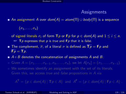

Boolean Constraints
Nogoods, Solutions, and Unit Propagation
A nogood is a set {σ1, . . . , σn} of signed literals,expressing a constraint violated by any assignmentcontaining σ1, . . . , σn.
An assignment A such that AT ∪ AF = dom(A) and AT ∩ AF = ∅is a solution for a set ∆ of nogoods, if δ 6⊆ A for all δ ∈ ∆.
For a nogood δ, a literal σ ∈ δ, and an assignment A, we say thatσ is unit-resulting for δ wrt A, if
1 δ \ A = {σ} and2 σ 6∈ A.
For a set ∆ of nogoods and an assignment A, unit propagation is theiterated process of extending A with unit-resulting literals until nofurther literal is unit-resulting for any nogood in ∆.
Torsten Schaub et al. (KRR@UP) Modeling and Solving in ASP 121 / 226

Nogoods from Logic Programs
Conflict-Driven Answer Set Solving:Overview
24 Motivation
25 Boolean Constraints
26 Nogoods from Logic ProgramsNogoods from program completionNogoods from loop formulas
27 Conflict-Driven Nogood LearningCDNL-ASP AlgorithmNogood PropagationConflict Analysis
Torsten Schaub et al. (KRR@UP) Modeling and Solving in ASP 122 / 226

Nogoods from Logic Programs Nogoods from program completion
Nogoods from logic programsvia program completion
The completion of a logic program Π can be defined as follows:
{pβ ↔ p1 ∧ · · · ∧ pm ∧ ¬pm+1 ∧ · · · ∧ ¬pn |β ∈ body(Π), β = {p1, . . . , pm, not pm+1, . . . , not pn}}
∪ {p ↔ pβ1 ∨ · · · ∨ pβk |p ∈ atom(Π), body(p) = {β1, . . . , βk}} ,
where body(p) = {body(r) | r ∈ Π, head(r) = p}.
Torsten Schaub et al. (KRR@UP) Modeling and Solving in ASP 123 / 226

Nogoods from Logic Programs Nogoods from program completion
Nogoods from logic programsvia program completion
Let β = {p1, . . . , pm, not pm+1, . . . , not pn} be a body.
The equivalence
pβ ↔ p1 ∧ · · · ∧ pm ∧ ¬pm+1 ∧ · · · ∧ ¬pn
can be decomposed into two implications.
1 We get
pβ → p1 ∧ · · · ∧ pm ∧ ¬pm+1 ∧ · · · ∧ ¬pn
which is equivalent to the conjunction of
¬pβ ∨ p1, . . . , ¬pβ ∨ pm, ¬pβ ∨ ¬pm+1, . . . , ¬pβ ∨ ¬pn
This set of clauses expresses the following set of nogoods:
∆(β) = { {Tβ,Fp1}, . . . , {Tβ,Fpm}, {Tβ,Tpm+1}, . . . , {Tβ,Tpn} }Torsten Schaub et al. (KRR@UP) Modeling and Solving in ASP 124 / 226

Nogoods from Logic Programs Nogoods from program completion
Nogoods from logic programsvia program completion
Let β = {p1, . . . , pm, not pm+1, . . . , not pn} be a body.
The equivalence
pβ ↔ p1 ∧ · · · ∧ pm ∧ ¬pm+1 ∧ · · · ∧ ¬pn
can be decomposed into two implications.
2 The converse of the previous implication, viz.
p1 ∧ · · · ∧ pm ∧ ¬pm+1 ∧ · · · ∧ ¬pn → pβ
gives rise to the nogood
δ(β) = {Fβ,Tp1, . . . ,Tpm,Fpm+1, . . . ,Fpn}
Intuitively, δ(β) is a constraint enforcing the truth of body β, or thefalsity of a contained literal.
Torsten Schaub et al. (KRR@UP) Modeling and Solving in ASP 125 / 226

Nogoods from Logic Programs Nogoods from program completion
Nogoods from logic programsvia program completion
Proceeding analogously with the atom-based equivalences, viz.
p ↔ pβ1 ∨ · · · ∨ pβk
we obtain for an atom p ∈ atom(Π) along with its bodiesbody(p) = {β1, . . . , βk} the nogoods
∆(p) = { {Fp,Tβ1}, . . . , {Fp,Tβk} } and δ(p) = {Tp,Fβ1, . . . ,Fβk} .
Torsten Schaub et al. (KRR@UP) Modeling and Solving in ASP 126 / 226

Nogoods from Logic Programs Nogoods from program completion
Nogoods from logic programsatom-oriented nogoods
For an atom p where body(p) = {β1, . . . , βk}, recall that
δ(p) = {Tp,Fβ1, . . . ,Fβk}∆(p) = { {Fp,Tβ1}, . . . , {Fp,Tβk} } .
For example, for atom x with body(x) = {{y}, {not z}}, we obtain
x ← yx ← not z
δ(x) = {Tx ,F{y},F{not z}}∆(x) = { {Fx ,T{y}}, {Fx ,T{not z}} }
For nogood δ(x) = {Tx ,F{y},F{not z}}, the signed literal
Fx is unit-resulting wrt assignment (F{y},F{not z}) and
T{not z} is unit-resulting wrt assignment (Tx ,F{y})
Torsten Schaub et al. (KRR@UP) Modeling and Solving in ASP 127 / 226
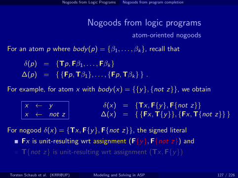

Nogoods from Logic Programs Nogoods from program completion
Nogoods from logic programsbody-oriented nogoods
For a body β = {p1, . . . , pm, not pm+1, . . . , not pn}, recall that
δ(β) = {Fβ,Tp1, . . . ,Tpm,Fpm+1, . . . ,Fpn}∆(β) = { {Tβ,Fp1}, . . . , {Tβ,Fpm}, {Tβ,Tpm+1}, . . . , {Tβ,Tpn} } .
For example, for body {x , not y}, we obtain
. . .← x , not y...
. . .← x , not y
δ({x , not y}) = {F{x , not y},Tx ,Fy}∆({x , not y}) = { {T{x , not y},Fx}, {T{x , not y},Ty} }
For nogood δ({x , not y}) = {F{x , not y},Tx ,Fy}, the signed literal
T{x , not y} is unit-resulting wrt assignment (Tx ,Fy) and
Ty is unit-resulting wrt assignment (F{x , not y},Tx).
Torsten Schaub et al. (KRR@UP) Modeling and Solving in ASP 128 / 226

Nogoods from Logic Programs Nogoods from program completion
Characterization of answer setsfor tight logic programs
Let Π be a logic program and
∆Π = {δ(p) | p ∈ atom(Π)} ∪ {δ ∈ ∆(p) | p ∈ atom(Π)}∪ {δ(β) | β ∈ body(Π)} ∪ {δ ∈ ∆(β) | β ∈ body(Π)} .
Theorem
Let Π be a tight logic program. Then,X ⊆ atom(Π) is an answer set of Π iffX = AT ∩ atom(Π) for a (unique) solution A for ∆Π.
Torsten Schaub et al. (KRR@UP) Modeling and Solving in ASP 129 / 226

Nogoods from Logic Programs Nogoods from program completion
Characterization of answer setsfor tight logic programs, ie. free of positive recursion
Let Π be a logic program and
∆Π = {δ(p) | p ∈ atom(Π)} ∪ {δ ∈ ∆(p) | p ∈ atom(Π)}∪ {δ(β) | β ∈ body(Π)} ∪ {δ ∈ ∆(β) | β ∈ body(Π)} .
Theorem
Let Π be a tight logic program. Then,X ⊆ atom(Π) is an answer set of Π iffX = AT ∩ atom(Π) for a (unique) solution A for ∆Π.
Torsten Schaub et al. (KRR@UP) Modeling and Solving in ASP 129 / 226

Nogoods from Logic Programs Nogoods from loop formulas
Nogoods from logic programsvia loop formulas
Let Π be a normal logic program and recall that:
For L ⊆ atom(Π), the external supports of L for Π are
ESΠ(L) = {r ∈ Π | head(r) ∈ L, body(r)+ ∩ L = ∅}.The (disjunctive) loop formula of L for Π is
LF Π(L) =(∨
A∈LA)→(∨
r∈ESΠ(L)body(r))
≡(∧
r∈ESΠ(L)¬body(r))→(∧
A∈L¬A)
+ The loop formula of L enforces all atoms in L to be falsewhenever L is not externally supported.
The external bodies of L for Π are
EB(L) = {body(r) | r ∈ ESΠ(L)}
Torsten Schaub et al. (KRR@UP) Modeling and Solving in ASP 130 / 226

Nogoods from Logic Programs Nogoods from loop formulas
Nogoods from logic programsloop nogoods
For a logic program Π and some ∅ ⊂ U ⊆ atom(Π),define the loop nogood of an atom p ∈ U as
λ(p,U) = {Tp,Fβ1, . . . ,Fβk}where EB(U) = {β1, . . . , βk}.In all, we get the following set of loop nogoods for Π:
ΛΠ =⋃∅⊂U⊆atom(Π){λ(p,U) | p ∈ U}
The set ΛΠ of loop nogoods denies cyclic support among true atoms.
Torsten Schaub et al. (KRR@UP) Modeling and Solving in ASP 131 / 226

Nogoods from Logic Programs Nogoods from loop formulas
Example
Consider
Π =
x ← not yy ← not x
u ← xu ← vv ← u, y
For u in the set {u, v}, we obtain the loop nogood:
λ(u, {u, v}) = {Tu,F{x}}
Similarly for v in {u, v}, we get:
λ(v , {u, v}) = {Tv ,F{x}}
Torsten Schaub et al. (KRR@UP) Modeling and Solving in ASP 132 / 226

Nogoods from Logic Programs Nogoods from loop formulas
Characterization of answer sets
Theorem
Let Π be a logic program. Then,X ⊆ atom(Π) is an answer set of Π iffX = AT ∩ atom(Π) for a (unique) solution A for ∆Π ∪ ΛΠ.
Some remarks
Nogoods in ΛΠ augment ∆Π with conditions checkingfor unfounded sets, in particular, those being loops.While |∆Π| is linear in the size of Π, ΛΠ may containexponentially many (non-redundant) loop nogoods
Torsten Schaub et al. (KRR@UP) Modeling and Solving in ASP 133 / 226

Conflict-Driven Nogood Learning
Conflict-Driven Answer Set Solving:Overview
24 Motivation
25 Boolean Constraints
26 Nogoods from Logic ProgramsNogoods from program completionNogoods from loop formulas
27 Conflict-Driven Nogood LearningCDNL-ASP AlgorithmNogood PropagationConflict Analysis
Torsten Schaub et al. (KRR@UP) Modeling and Solving in ASP 134 / 226

Conflict-Driven Nogood Learning
Conflict-driven search
Boolean constraint solving algorithms pioneered for SAT led to:
Traditional DPLL-style approach
(Unit) propagation(Chronological) backtracking
Modern CDCL-style approach
(Unit) propagationConflict analysis (via resolution)Learning + Backjumping + Assertion
Torsten Schaub et al. (KRR@UP) Modeling and Solving in ASP 135 / 226

Conflict-Driven Nogood Learning
DPLL-style solving
loop
propagate // compute deterministic consequences
if no conflict thenif all variables assigned then return variable assignmentelse decide // non-deterministically assign some literal
elseif top-level conflict then return unsatisfiableelse
backtrack // undo assignments made after last decisionflip // assign complement of last decision literal
Torsten Schaub et al. (KRR@UP) Modeling and Solving in ASP 136 / 226

Conflict-Driven Nogood Learning
CDCL-style solving
loop
propagate // compute deterministic consequences
if no conflict thenif all variables assigned then return variable assignmentelse decide // non-deterministically assign some literal
elseif top-level conflict then return unsatisfiableelse
analyze // analyze conflict and add a conflict constraintbackjump // undo assignments until conflict constraint is unit
Torsten Schaub et al. (KRR@UP) Modeling and Solving in ASP 137 / 226

Conflict-Driven Nogood Learning CDNL-ASP Algorithm
Outline of CDNL-ASP algorithm
Keep track of deterministic consequences by unit propagation on:
Program completion [∆Π]Loop nogoods, determined and recorded on demand [ΛΠ]
+ Dedicated unfounded set detection !
Dynamic nogoods, derived from conflicts and unfounded sets [∇]
When a nogood in ∆Π ∪∇ becomes violated:
Analyze the conflict by resolution(until reaching a Unique Implication Point, short: UIP)Learn the derived conflict nogood δBackjump to the earliest (heuristic) choice such that thecomplement of the UIP is unit-resulting for δAssert the complement of the UIP and proceed(by unit propagation)
Terminate when either:
Finding an answer set (a solution for ∆Π ∪ ΛΠ)Deriving a conflict independently of (heuristic) choices
Torsten Schaub et al. (KRR@UP) Modeling and Solving in ASP 138 / 226

Conflict-Driven Nogood Learning CDNL-ASP Algorithm
Algorithm 1: CDNL-ASPInput : A logic program Π.Output : An answer set of Π or “no answer set”.
A← ∅ // assignment over atom(Π) ∪ body(Π)∇ ← ∅ // set of (dynamic) nogoodsdl ← 0 // decision levelloop
(A,∇)← NogoodPropagation(Π,∇,A)if ε ⊆ A for some ε ∈ ∆Π ∪∇ then
if dl = 0 then return no answer set(δ, k)← ConflictAnalysis(ε,Π,∇,A)∇ ← ∇∪ {δ} // learningA← (A \ {σ ∈ A | k < dl(σ)}) // backjumpingdl ← k
else if AT ∪ AF = atom(Π) ∪ body(Π) thenreturn AT ∩ atom(Π) // answer set
elseσd ← Select(Π,∇,A) // heuristic choice of σd /∈ Adl ← dl + 1A← A ◦ (σd) // dl(σd) = dl
Torsten Schaub et al. (KRR@UP) Modeling and Solving in ASP 139 / 226

Conflict-Driven Nogood Learning CDNL-ASP Algorithm
Observations
Decision level dl , initially set to 0, is used to count the number ofheuristically chosen literals in assignment A.
For a heuristically chosen literal σd = Tp or σd = Fp, respectively, werequire p ∈ (atom(Π) ∪ body(Π)) \ (AT ∪ AF).
For any literal σ ∈ A, dl(σ) denotes the decision level of σ, viz. thevalue dl had when σ was assigned.
A conflict is detected from violation of a nogood ε ⊆ ∆Π ∪∇.
A conflict at decision level 0 (where A contains no heuristicallychosen literals) indicates non-existence of answer sets.
A nogood δ derived by conflict analysis is asserting, that is,some literal is unit-resulting for δ at a decision level k < dl .
After learning δ and backjumping to decision level k,at least one literal is newly derivable by unit propagation.No explicit flipping of heuristically chosen literals !
Torsten Schaub et al. (KRR@UP) Modeling and Solving in ASP 140 / 226
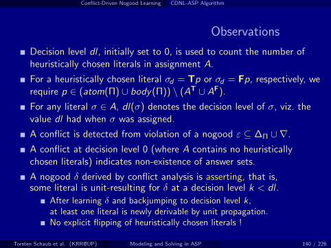

Conflict-Driven Nogood Learning CDNL-ASP Algorithm
Example: CDNL-ASP
Consider
Π =
{x ← not yy ← not x
u ← x , yu ← v
v ← xv ← u, y
w ← not x , not y}
dl σd σ δ
1 Tu
2 F{not x , not y}Fw {Tw ,F{not x , not y}} = δ(w)
3 F{not y}Fx {Tx ,F{not y}} = δ(x)F{x} {T{x},Fx} ∈ ∆({x})F{x , y} {T{x , y},Fx} ∈ ∆({x , y})...
...{Tu,F{x},F{x , y}} = λ(u, {u, v}) 8
Torsten Schaub et al. (KRR@UP) Modeling and Solving in ASP 141 / 226

Conflict-Driven Nogood Learning CDNL-ASP Algorithm
Example: CDNL-ASP
Consider
Π =
{x ← not yy ← not x
u ← x , yu ← v
v ← xv ← u, y
w ← not x , not y}
dl σd σ δ
1 TuTx {Tu,Fx} ∈ ∇...
...Tv {Fv ,T{x}} ∈ ∆(v)Fy {Ty ,F{not x}} = δ(y)Fw {Tw ,F{not x , not y}} = δ(w)
Torsten Schaub et al. (KRR@UP) Modeling and Solving in ASP 142 / 226

Conflict-Driven Nogood Learning Nogood Propagation
Outline of NogoodPropagation
Derive deterministic consequences via:
Unit propagation on ∆Π and ∇;Unfounded sets U ⊆ atom(Π).
Note that U is unfounded if EB(U) ⊆ AF.
+ For any p ∈ U, we have (λ(p,U) \ {Tp}) ⊆ A.
An “interesting” unfounded set U satisfies:
∅ ⊂ U ⊆ (atom(Π) \ AF) .
Wrt a fixpoint of unit propagation,such an unfounded set contains some loop of Π.
å Tight programs do not yield “interesting” unfounded sets !
Given an unfounded set U and some p ∈ U, adding λ(p,U) to ∇triggers a conflict or further derivations by unit propagation.
+ Add loop nogoods atom by atom to eventually falsify all p ∈ U.
Torsten Schaub et al. (KRR@UP) Modeling and Solving in ASP 143 / 226

Conflict-Driven Nogood Learning Nogood Propagation
Algorithm 2: NogoodPropagationInput : A logic program Π, a set ∇ of nogoods, and an assignment A.Output : An extended assignment and set of nogoods.
U ← ∅ // set of unfounded atomsloop
repeatif δ ⊆ A for some δ ∈ ∆Π ∪∇ then return (A,∇) // conflictΣ← {δ ∈ ∆Π ∪∇ | (δ \ A) = {σ}, σ /∈ A} // unit-resulting nogoodsif Σ 6= ∅ then
let σ ∈ (δ \ A) for some δ ∈ Σ inA← A ◦ (σ) // dl(σ) = max({dl(ρ) | ρ ∈ (δ \ {σ})} ∪ {0})
until Σ = ∅
if Π is tight then return (A,∇) // no unfounded set ∅ ⊂ U ⊆ (atom(Π) \ AF)else
U ← (U \ AF)if U = ∅ then U ← UnfoundedSet(Π,A)
if U = ∅ then return (A,∇)// no unfounded set ∅ ⊂ U ⊆ (atom(Π) \ AF)let p ∈ U in∇ ← ∇∪ {λ(p,U)} // record unit-resulting or violated loop nogood
Torsten Schaub et al. (KRR@UP) Modeling and Solving in ASP 144 / 226

Conflict-Driven Nogood Learning Nogood Propagation
Requirements for UnfoundedSet
Implementations of UnfoundedSet must guarantee the following for aresult U
1 U ⊆ (atom(Π) \ AF)2 EB(U) ⊆ AF
3 U = ∅ iff there is no nonempty unfounded subset of (atom(Π) \ AF)
Beyond that, there are various alternatives, such as:
Calculating the greatest unfounded setCalculating unfounded sets within strongly connected components ofthe positive atom dependency graph of Π
Usually, the latter option is implemented in ASP solvers
Torsten Schaub et al. (KRR@UP) Modeling and Solving in ASP 145 / 226

Conflict-Driven Nogood Learning Nogood Propagation
Example: NogoodPropagation
Consider
Π =
{x ← not yy ← not x
u ← x , yu ← v
v ← xv ← u, y
w ← not x , not y}
dl σd σ δ
1 Tu
2 F{not x , not y}Fw {Tw ,F{not x , not y}} = δ(w)
3 F{not y}Fx {Tx ,F{not y}} = δ(x)F{x} {T{x},Fx} ∈ ∆({x})F{x , y} {T{x , y},Fx} ∈ ∆({x , y})T{not x} {F{not x},Fx} = δ({not x})Ty {F{not y},Fy} = δ({not y})T{v} {Tu,F{x , y},F{v}} = δ(u)T{u, y} {F{u, y},Tu,Ty} = δ({u, y})Tv {Fv ,T{u, y}} ∈ ∆(v)
{Tu,F{x},F{x , y}} = λ(u, {u, v}) 8
Torsten Schaub et al. (KRR@UP) Modeling and Solving in ASP 146 / 226

Conflict-Driven Nogood Learning Conflict Analysis
Outline of ConflictAnalysis
Conflict analysis is triggered whenever some nogood δ ∈ ∆Π ∪∇becomes violated, viz. δ ⊆ A, at a decision level dl > 0.
Note that all but the first literal assigned at dl have been unit-resultingfor nogoods ε ∈ ∆Π ∪∇.If σ ∈ δ has been unit-resulting for ε, we obtain a new violated nogoodby resolving δ and ε as follows:
(δ \ {σ}) ∪ (ε \ {σ}) .
Resolution is directed by resolving first over the literal σ ∈ δ derivedlast, viz. (δ \ A[σ]) = {σ}.
Iterated resolution progresses in inverse order of assignment.
Iterated resolution stops as soon as it generates a nogood δcontaining exactly one literal σ assigned at decision level dl .
This literal σ is called First Unique Implication Point (First-UIP).All literals in (δ \ {σ}) are assigned at decision levels smaller than dl .
Torsten Schaub et al. (KRR@UP) Modeling and Solving in ASP 147 / 226

Conflict-Driven Nogood Learning Conflict Analysis
Algorithm 3: ConflictAnalysisInput : A violated nogood δ, a logic program Π, a set ∇ of nogoods, and
an assignment A.Output : A derived nogood and a decision level.
looplet σ ∈ δ such that (δ \ A[σ]) = {σ} in
k ← max({dl(ρ) | ρ ∈ δ \ {σ}} ∪ {0})if k = dl(σ) then
let ε ∈ ∆Π ∪∇ such that (ε \ A[σ]) = {σ} inδ ← (δ \ {σ}) ∪ (ε \ {σ}) // resolution
else return (δ, k)
Torsten Schaub et al. (KRR@UP) Modeling and Solving in ASP 148 / 226

Conflict-Driven Nogood Learning Conflict Analysis
Example: ConflictAnalysis
Consider
Π =
{x ← not yy ← not x
u ← x , yu ← v
v ← xv ← u, y
w ← not x , not y}
dl σd σ δ1 Tu2 F{not x , not y}
Fw {Tw ,F{not x , not y}} = δ(w)3 F{not y}
Fx {Tx ,F{not y}} = δ(x)F{x} {T{x},Fx} ∈ ∆({x}) {Tu,Fx}F{x , y} {T{x , y},Fx} ∈ ∆({x , y}) {Tu,Fx ,F{x}}T{not x} {F{not x},Fx} = δ({not x})Ty {F{not y},Fy} = δ({not y})T{v} {Tu,F{x , y},F{v}} = δ(u)T{u, y} {F{u, y},Tu,Ty} = δ({u, y})Tv {Fv ,T{u, y}} ∈ ∆(v)
{Tu,F{x},F{x , y}} = λ(u, {u, v}) 8
Torsten Schaub et al. (KRR@UP) Modeling and Solving in ASP 149 / 226

Conflict-Driven Nogood Learning Conflict Analysis
Remarks
There always is a First-UIP at which conflict analysis terminates.
In the worst, resolution stops at the heuristically chosen literalassigned at decision level dl .
The nogood δ containing First-UIP σ is violated by A, viz. δ ⊆ A.
We have k = max({dl(ρ) | ρ ∈ δ \ {σ}} ∪ {0}) < dl .
After recording δ in ∇ and backjumping to decision level k,σ is unit-resulting for δ !Such a nogood δ is called asserting.
Asserting nogoods direct conflict-driven search into a different regionof the search space than traversed before,without explicitly flipping any heuristically chosen literal !
Torsten Schaub et al. (KRR@UP) Modeling and Solving in ASP 150 / 226

Effective Modeling: Overview
28 Problems as Logic Programs (Revisited)Graph ColoringHamiltonian CycleTraveling Salesperson
29 Encoding MethodologyTweaking N-QueensDo’s and Dont’s
30 Hints
Torsten Schaub et al. (KRR@UP) Modeling and Solving in ASP 151 / 226

Problems as Logic Programs (Revisited)
Effective Modeling: Overview
28 Problems as Logic Programs (Revisited)Graph ColoringHamiltonian CycleTraveling Salesperson
29 Encoding MethodologyTweaking N-QueensDo’s and Dont’s
30 Hints
Torsten Schaub et al. (KRR@UP) Modeling and Solving in ASP 152 / 226

Problems as Logic Programs (Revisited)
Modeling and Interpreting
Problem
Logic Program
Solution
Stable Models?
-
6
Modeling Interpreting
Solving
Torsten Schaub et al. (KRR@UP) Modeling and Solving in ASP 153 / 226

Problems as Logic Programs (Revisited)
Modeling and Interpreting
Problem
Logic Program
Solution
Stable Models?
-
6
Modeling Interpreting
Solving
Torsten Schaub et al. (KRR@UP) Modeling and Solving in ASP 153 / 226
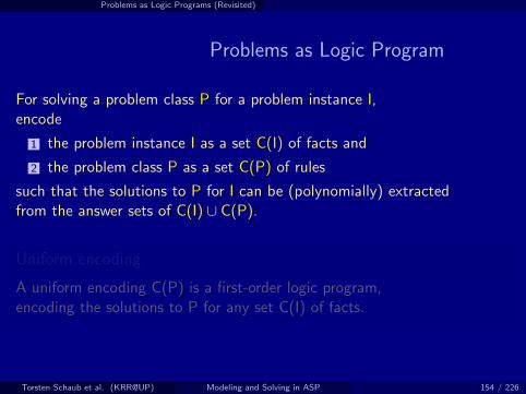
Problems as Logic Programs (Revisited)
Problems as Logic Program
For solving a problem class P for a problem instance I,encode
1 the problem instance I as a set C(I) of facts and
2 the problem class P as a set C(P) of rules
such that the solutions to P for I can be (polynomially) extractedfrom the answer sets of C(I) ∪ C(P).
Uniform encoding
A uniform encoding C(P) is a first-order logic program,encoding the solutions to P for any set C(I) of facts.
Torsten Schaub et al. (KRR@UP) Modeling and Solving in ASP 154 / 226

Problems as Logic Programs (Revisited) Graph Coloring
N-ColorabilityProblem Instance as Facts
Given: a (directed) graph G
G =
V = {1, 2, 3, 4, 5, 6},E = {(1, 2), (1, 3), (1, 4),
(2, 4), (2, 5), (2, 6),(3, 1), (3, 4), (3, 5),(4, 1), (4, 2),(5, 3), (5, 4), (5, 6),(6, 2), (6, 3), (6, 5)}
� ��1
� ��3
� ��4
� ��6� ��2
� ��5
-
6
@@@@R
��
��
6
QQk
?
z
-
@@@@I
�����
�
9
��
��+
QQQQs
QQk
����3
Torsten Schaub et al. (KRR@UP) Modeling and Solving in ASP 155 / 226

Problems as Logic Programs (Revisited) Graph Coloring
N-ColorabilityProblem Instance as Facts
Given: a (directed) graph G
node(1). node(2). node(3).
node(4). node(5). node(6).
edge(1,2). edge(1,3). edge(1,4).
edge(2,4). edge(2,5). edge(2,6).
edge(3,1). edge(3,4). edge(3,5).
edge(4,1). edge(4,2). edge(5,3).
edge(5,4). edge(5,6). edge(6,2).
edge(6,3). edge(6,5).
� ��1
� ��3
� ��4
� ��6� ��2
� ��5
-
6
@@@@R
��
��
6
QQk
?
z
-
@@@@I
�����
�
9
��
��+
QQQQs
QQk
����3
Torsten Schaub et al. (KRR@UP) Modeling and Solving in ASP 155 / 226

Problems as Logic Programs (Revisited) Graph Coloring
N-Colorability(Extended) Problem Encoding
Natural Language
1 Each node has a unique color.
2 Any two connected nodesmust not have the same color.
3 Let there be three colors.
4 A solution is a coloring.
Logical Language
1 color(X,C) :- iscol(C),
node(X), not other(X,C).
other(X,C) :- iscol(C),
color(X,D), D != C.
2 :- color(X,C), color(Y,C),
edge(X,Y).
3 #const n=3.
iscol(1..n).
4 #hide.
#show color/2.
Torsten Schaub et al. (KRR@UP) Modeling and Solving in ASP 156 / 226

Problems as Logic Programs (Revisited) Graph Coloring
N-Colorability(Extended) Problem Encoding
Natural Language
1 Each node has a unique color.
2 Any two connected nodesmust not have the same color.
3 Let there be three colors.
4 A solution is a coloring.
Logical Language
1 1 #count{ color(X,C) :
iscol(C) } 1
:- node(X).
2 :- color(X,C), color(Y,C),
edge(X,Y).
3 #const n=3.
iscol(1..n).
4 #hide.
#show color/2.
Torsten Schaub et al. (KRR@UP) Modeling and Solving in ASP 156 / 226

Problems as Logic Programs (Revisited) Graph Coloring
N-ColorabilityRecapitulation I
Instance as Facts (in graph.lp)
node(1). node(2). node(3). node(4). node(5). node(6).
edge(1,2). edge(1,3). edge(1,4).
edge(2,4). edge(2,5). edge(2,6).
edge(3,1). edge(3,4). edge(3,5).
edge(4,1). edge(4,2).
edge(5,3). edge(5,4). edge(5,6).
edge(6,2). edge(6,3). edge(6,5).
Torsten Schaub et al. (KRR@UP) Modeling and Solving in ASP 157 / 226
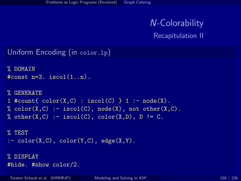
Problems as Logic Programs (Revisited) Graph Coloring
N-ColorabilityRecapitulation II
Uniform Encoding (in color.lp)
% DOMAIN
#const n=3. iscol(1..n).
% GENERATE
1 #count{ color(X,C) : iscol(C) } 1 :- node(X).
% color(X,C) :- iscol(C), node(X), not other(X,C).
% other(X,C) :- iscol(C), color(X,D), D != C.
% TEST
:- color(X,C), color(Y,C), edge(X,Y).
% DISPLAY
#hide. #show color/2.
Torsten Schaub et al. (KRR@UP) Modeling and Solving in ASP 158 / 226

Problems as Logic Programs (Revisited) Graph Coloring
N-ColorabilityLet’s Run it!
gringo graph.lp color.lp | clasp 0
clasp version 2.0.2
Reading from stdin
Solving...
Answer: 1
color(6,2) color(5,3) color(4,2) color(3,1) color(2,1) color(1,3)
Answer: 2
color(6,1) color(5,3) color(4,1) color(3,2) color(2,2) color(1,3)
Answer: 3
color(6,3) color(5,2) color(4,3) color(3,1) color(2,1) color(1,2)
Answer: 4
color(6,1) color(5,2) color(4,1) color(3,3) color(2,3) color(1,2)
Answer: 5
color(6,3) color(5,1) color(4,3) color(3,2) color(2,2) color(1,1)
Answer: 6
color(6,2) color(5,1) color(4,2) color(3,3) color(2,3) color(1,1)
Torsten Schaub et al. (KRR@UP) Modeling and Solving in ASP 159 / 226

Problems as Logic Programs (Revisited) Graph Coloring
N-ColorabilityLet’s Interpret it!
Found: 3-coloring(s)
Answer: 1
color(1,3) color(5,3)
color(2,1) color(3,1)
color(4,2) color(6,2) � ��1
� ��3
� ��4
� ��6� ��2
� ��5
-
6
@@@@R
��
��
6
QQk
?
z
-
@@
@@I
�����
�
9
��
��+
QQQQs
QQk
����3
Torsten Schaub et al. (KRR@UP) Modeling and Solving in ASP 160 / 226

Problems as Logic Programs (Revisited) Graph Coloring
N-ColorabilityLet’s Interpret it!
Found: 3-coloring(s)
Answer: 1
color(1,3) color(5,3)
color(2,1) color(3,1)
color(4,2) color(6,2)~1
� ��3
� ��4
� ��6� ��2
~5
-
6
@@@@R
��
��
6
QQk
?
z
-
@@
@@I
�����
�
9
��
��+
QQQQs
QQk
����3
Torsten Schaub et al. (KRR@UP) Modeling and Solving in ASP 160 / 226

Problems as Logic Programs (Revisited) Graph Coloring
N-ColorabilityLet’s Interpret it!
Found: 3-coloring(s)
Answer: 1
color(1,3) color(5,3)
color(2,1) color(3,1)
color(4,2) color(6,2)~1
~3
� ��4
� ��6~2
~5
-
6
@@@@R
��
��
6
QQk
?
z
-
@@
@@I
�����
�
9
��
��+
QQQQs
QQk
����3
Torsten Schaub et al. (KRR@UP) Modeling and Solving in ASP 160 / 226

Problems as Logic Programs (Revisited) Graph Coloring
N-ColorabilityLet’s Interpret it!
Found: 3-coloring(s)
Answer: 1
color(1,3) color(5,3)
color(2,1) color(3,1)
color(4,2) color(6,2)~1
~3
~4
~6~2
~5
-
6
@@@@R
��
��
6
QQk
?
z
-
@@
@@I
�����
�
9
��
��+
QQQQs
QQk
����3
Torsten Schaub et al. (KRR@UP) Modeling and Solving in ASP 160 / 226

Problems as Logic Programs (Revisited) Graph Coloring
Interlude: Answer Set(s) Computation
ProblemInstance
ProblemEncoding
�� ��GrounderPropositional
Logic Program
�� ��Solver
Stable Models
6
- -
6
? Grounding
Solving
Torsten Schaub et al. (KRR@UP) Modeling and Solving in ASP 161 / 226

Problems as Logic Programs (Revisited) Graph Coloring
Interlude: Answer Set(s) Computation
ProblemInstance
ProblemEncoding
�� ��GrounderPropositional
Logic Program
�� ��Solver
Stable Models
6
- -
6
? Grounding
Solving
Torsten Schaub et al. (KRR@UP) Modeling and Solving in ASP 161 / 226
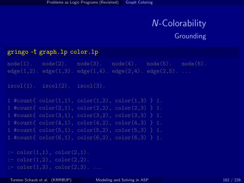
Problems as Logic Programs (Revisited) Graph Coloring
N-ColorabilityGrounding
gringo -t graph.lp color.lp
node(1). node(2). node(3). node(4). node(5). node(6).
edge(1,2). edge(1,3). edge(1,4). edge(2,4). edge(2,5). ...
iscol(1). iscol(2). iscol(3).
1 #count{ color(1,1), color(1,2), color(1,3) } 1.
1 #count{ color(2,1), color(2,2), color(2,3) } 1.
1 #count{ color(3,1), color(3,2), color(3,3) } 1.
1 #count{ color(4,1), color(4,2), color(4,3) } 1.
1 #count{ color(5,1), color(5,2), color(5,3) } 1.
1 #count{ color(6,1), color(6,2), color(6,3) } 1.
:- color(1,1), color(2,1).
:- color(1,2), color(2,2).
:- color(1,3), color(2,3). ...
Torsten Schaub et al. (KRR@UP) Modeling and Solving in ASP 162 / 226

Problems as Logic Programs (Revisited) Graph Coloring
N-ColorabilitySolving
gringo graph.lp color.lp | clasp --stats 0
...
Models : 6
Time : 0.001s (Solving: 0.00s 1st Model: 0.00s Unsat: 0.00s)
CPU Time : 0.000s
Choices : 5
Conflicts : 0
Restarts : 0
Atoms : 63
Rules : 113 (1: 95 2: 12 3: 6)
Bodies : 64
Equivalences: 106 (Atom=Atom: 31 Body=Body: 6 Other: 69)
Tight : Yes
Variables : 63 (Eliminated: 0 Frozen: 30)
Constraints : 45 (Binary: 73.3% Ternary: 0.0% Other: 26.7%)
Lemmas : 0 (Binary: 0.0% Ternary: 0.0% Other: 0.0%)
Torsten Schaub et al. (KRR@UP) Modeling and Solving in ASP 163 / 226

Problems as Logic Programs (Revisited) Hamiltonian Cycle
Hamiltonian CycleProblem Instance as Facts
Recall: a directed graph G
node(1). node(2). node(3).
node(4). node(5). node(6).
edge(1,2). edge(1,3). edge(1,4).
edge(2,4). edge(2,5). edge(2,6).
edge(3,1). edge(3,4). edge(3,5).
edge(4,1). edge(4,2). edge(5,3).
edge(5,4). edge(5,6). edge(6,2).
edge(6,3). edge(6,5).
� ��1
� ��3
� ��4
� ��6� ��2
� ��5
-
6
@@@@R
����
6
QQQQk
?
z
-
@@
@@I
�����
�
9
����+
QQQQs
QQQQk
����3
Torsten Schaub et al. (KRR@UP) Modeling and Solving in ASP 164 / 226

Problems as Logic Programs (Revisited) Hamiltonian Cycle
Hamiltonian CycleEngineering an Encoding
Problem Specification
A (directed) graph G = (V ,E ) is Hamiltonian if it containsa cycle C that visits every node of V exactly once.
+ C traverses exactly one incoming and one outgoing edge per node.+ C traverses every node of V (starting from an arbitrary node in V ).
Problem Encoding
1 #count{ cycle(X,Y) : edge(X,Y) } 1 :- node(Y).
1 #count{ cycle(X,Y) : edge(X,Y) } 1 :- node(X).
Torsten Schaub et al. (KRR@UP) Modeling and Solving in ASP 165 / 226

Problems as Logic Programs (Revisited) Hamiltonian Cycle
Hamiltonian CycleEngineering an Encoding
Problem Specification
A (directed) graph G = (V ,E ) is Hamiltonian if it containsa cycle C that visits every node of V exactly once.
+ C traverses exactly one incoming and one outgoing edge per node.+ C traverses every node of V (starting from an arbitrary node in V ).
Problem Encoding
reach(X) :- first(X).
reach(Y) :- reach(X), cycle(X,Y).
+ The definition of reach is recursive!
Torsten Schaub et al. (KRR@UP) Modeling and Solving in ASP 165 / 226

Problems as Logic Programs (Revisited) Hamiltonian Cycle
Hamiltonian CycleEngineering an Encoding
Problem Specification
A (directed) graph G = (V ,E ) is Hamiltonian if it containsa cycle C that visits every node of V exactly once.
+ C traverses exactly one incoming and one outgoing edge per node.+ C traverses every node of V (starting from an arbitrary node in V ).
Problem Encoding
reach(X) :- first(X).
reach(Y) :- reach(X), cycle(X,Y).
first(X) :- X = #min[ node(Y) = Y ].
Torsten Schaub et al. (KRR@UP) Modeling and Solving in ASP 165 / 226

Problems as Logic Programs (Revisited) Hamiltonian Cycle
Hamiltonian CycleEngineering an Encoding
Problem Specification
A (directed) graph G = (V ,E ) is Hamiltonian if it containsa cycle C that visits every node of V exactly once.
+ C traverses exactly one incoming and one outgoing edge per node.+ C traverses every node of V (starting from an arbitrary node in V ).
Problem Encoding
reach(X) :- first(X).
reach(Y) :- reach(X), cycle(X,Y).
:- node(Y), not reach(Y).
Torsten Schaub et al. (KRR@UP) Modeling and Solving in ASP 165 / 226

Problems as Logic Programs (Revisited) Hamiltonian Cycle
Hamiltonian CycleThe Complete Picture
Uniform Encoding (in cycle.lp)
% DOMAIN
first(X) :- X = #min[ node(Y) = Y ].
% GENERATE
1 #count{ cycle(X,Y) : edge(X,Y) } 1 :- node(X).
1 #count{ cycle(X,Y) : edge(X,Y) } 1 :- node(Y).
% DEFINE
reach(X) :- first(X).
reach(Y) :- reach(X), cycle(X,Y).
% TEST
:- node(Y), not reach(Y).
% DISPLAY
#hide. #show cycle/2.
Torsten Schaub et al. (KRR@UP) Modeling and Solving in ASP 166 / 226

Problems as Logic Programs (Revisited) Hamiltonian Cycle
Hamiltonian CycleLet’s Run it!
gringo graph.lp cycle.lp | clasp --stats
Answer: 1
cycle(6,5) cycle(5,3) cycle(4,2) cycle(3,1) cycle(2,6) cycle(1,4)
SATISFIABLE
Models : 1+
Time : 0.001s (Solving: 0.00s 1st Model: 0.00s Unsat: 0.00s)
CPU Time : 0.000s
Choices : 3
Conflicts : 0
Restarts : 0
Atoms : 84
Rules : 117 (1: 84 2: 21 3: 12)
Bodies : 81
Equivalences: 174 (Atom=Atom: 36 Body=Body: 12 Other: 126)
Tight : No (SCCs: 1 Nodes: 20)
Torsten Schaub et al. (KRR@UP) Modeling and Solving in ASP 167 / 226

Problems as Logic Programs (Revisited) Hamiltonian Cycle
Hamiltonian CycleLet’s Interpret it!
Found: Hamiltonian cycle
Answer: 1
cycle(1,4)
cycle(4,2)
cycle(2,6)
cycle(6,5)
cycle(5,3)
cycle(3,1)� ��1
� ��3
� ��4
� ��6� ��2
� ��5
-
6
��
��
6
z
-
@@
@@I
9
��
��+
QQQQs
QQk
@@@@R �
����
QQk
����3
�
?
Torsten Schaub et al. (KRR@UP) Modeling and Solving in ASP 168 / 226

Problems as Logic Programs (Revisited) Hamiltonian Cycle
Hamiltonian CycleLet’s Interpret it!
Found: Hamiltonian cycle
Answer: 1
cycle(1,4)
cycle(4,2)
cycle(2,6)
cycle(6,5)
cycle(5,3)
cycle(3,1)� ��1
� ��3
~4
� ��6~2
� ��5
-
6
��
��
6
z
-
@@
@@I
9
��
��+
QQQQs
QQk
@@@@R �
����
QQk
����3
�
?
Torsten Schaub et al. (KRR@UP) Modeling and Solving in ASP 168 / 226

Problems as Logic Programs (Revisited) Hamiltonian Cycle
Hamiltonian CycleLet’s Interpret it!
Found: Hamiltonian cycle
Answer: 1
cycle(1,4)
cycle(4,2)
cycle(2,6)
cycle(6,5)
cycle(5,3)
cycle(3,1)� ��1
� ��3
~4
~6~2
~5
-
6
��
��
6
z
-
@@
@@I
9
��
��+
QQQQs
QQk
@@@@R �
����
QQk
����3
�
?
Torsten Schaub et al. (KRR@UP) Modeling and Solving in ASP 168 / 226

Problems as Logic Programs (Revisited) Hamiltonian Cycle
Hamiltonian CycleLet’s Interpret it!
Found: Hamiltonian cycle
Answer: 1
cycle(1,4)
cycle(4,2)
cycle(2,6)
cycle(6,5)
cycle(5,3)
cycle(3,1)� ��1
~3
~4
~6~2
~5
-
6
��
��
6
z
-
@@
@@I
9
��
��+
QQQQs
QQk
@@@@R �
����
QQk
����3
�
?
Torsten Schaub et al. (KRR@UP) Modeling and Solving in ASP 168 / 226

Problems as Logic Programs (Revisited) Hamiltonian Cycle
Hamiltonian CycleLet’s Interpret it!
Found: Hamiltonian cycle
Answer: 1
cycle(1,4)
cycle(4,2)
cycle(2,6)
cycle(6,5)
cycle(5,3)
cycle(3,1)
~1
~3
~4
~6~2
~5
-
6
��
��
6
z
-
@@
@@I
9
��
��+
QQQQs
QQk
@@@@R �
����
QQk
����3
�
?
Torsten Schaub et al. (KRR@UP) Modeling and Solving in ASP 168 / 226

Problems as Logic Programs (Revisited) Traveling Salesperson
Mr Hamilton as Traveling SalespersonProblem Instance as Facts
Given: a directed graph G plus edge costs
node(1). node(2). node(3).
node(4). node(5). node(6).
edge(1,2). edge(1,3). edge(1,4).
edge(2,4). edge(2,5). edge(2,6).
edge(3,1). edge(3,4). edge(3,5).
edge(4,1). edge(4,2). edge(5,3).
edge(5,4). edge(5,6). edge(6,2).
edge(6,3). edge(6,5).
� ��1
� ��3
� ��4
� ��6� ��2
� ��5
-2
6
3
@@@@R
1�
���
2
6
2
QQQQk 4
?
z
2
-2
@@
@@I
�����
�
9
2
����+
1
QQQQs
QQQQk
3
����3
Torsten Schaub et al. (KRR@UP) Modeling and Solving in ASP 169 / 226

Problems as Logic Programs (Revisited) Traveling Salesperson
Mr Hamilton as Traveling SalespersonProblem Instance as Facts
Given: a directed graph G plus edge costs
cost(1,2,2).
cost(1,3,3). cost(3,1,3).
cost(1,4,1). cost(4,1,1).
cost(2,4,2). cost(4,2,2).
cost(2,5,2).
cost(2,6,4). cost(6,2,4).
cost(3,4,2).
cost(3,5,2). cost(5,3,2).
cost(5,4,2).
cost(5,6,1). cost(6,5,1).
cost(6,3,3).
� ��1
� ��3
� ��4
� ��6� ��2
� ��5
-2
6
3
@@@@R
1�
���
2
6
2
QQQQk 4
?
z
2
-2
@@
@@I
�����
�
9
2
����+
1
QQQQs
QQQQk
3
����3
Torsten Schaub et al. (KRR@UP) Modeling and Solving in ASP 169 / 226

Problems as Logic Programs (Revisited) Traveling Salesperson
Mr Hamilton as Traveling SalespersonSolution Optimization
Optimization Objective
A Hamiltonian cycle is optimal if its accumulated edge costs are minimal.
+ Use #minimize (and/or #maximize) to associate each answer set withobjective value(s).
Optimization Encoding
% OPTIMIZE
#minimize[ cycle(X,Y) : cost(X,Y,C) = C@1 ].
Target: minimal sum of costs C (at priority level 1) associated withinstances of cycle in an answer set
Torsten Schaub et al. (KRR@UP) Modeling and Solving in ASP 170 / 226

Problems as Logic Programs (Revisited) Traveling Salesperson
Mr Hamilton as Traveling SalespersonLet’s Run it!
gringo graph.lp costs.lp cycle.lp price.lp | clasp --stats 0
Answer: 1
cycle(6,5) cycle(5,3) cycle(4,2) cycle(3,1) cycle(2,6) cycle(1,4)
Optimization: 13
Answer: 2
cycle(6,5) cycle(5,3) cycle(4,1) cycle(3,4) cycle(2,6) cycle(1,2)
Optimization: 12
Answer: 3
cycle(6,3) cycle(5,6) cycle(4,1) cycle(3,4) cycle(2,5) cycle(1,2)
Optimization: 11
OPTIMUM FOUND
Models : 1
Enumerated: 3
Optimum : yes
Optimization: 11
Time : 0.004s (Solving: 0.00s 1st Model: 0.00s Unsat: 0.00s)
CPU Time : 0.000s
Torsten Schaub et al. (KRR@UP) Modeling and Solving in ASP 171 / 226

Problems as Logic Programs (Revisited) Traveling Salesperson
Mr Hamilton as Traveling SalespersonLet’s Interpret it!
Found: optimal Hamiltonian cycle
Answer: 1
cycle(1,4)
cycle(4,2)
cycle(2,6)
cycle(6,5)
cycle(5,3)
cycle(3,1)� ��1
� ��3
� ��4
� ��6� ��2
� ��5
9
2QQ
QQkQQQQs
4
6
?
3
��
�������
2
-� 2
��
��+����31
-2
@@
@@I@@@@R
1
z
2
6
2QQ
QQk 3
Torsten Schaub et al. (KRR@UP) Modeling and Solving in ASP 172 / 226

Problems as Logic Programs (Revisited) Traveling Salesperson
Mr Hamilton as Traveling SalespersonLet’s Interpret it!
Found: optimal Hamiltonian cycle
Answer: 2
cycle(1,2)
cycle(2,6)
cycle(6,5)
cycle(5,3)
cycle(3,4)
cycle(4,1)� ��1
� ��3
� ��4
� ��6� ��2
� ��5
9
2QQ
QQkQQQQs
4
6
?
3
��
�������
2
-� 2
��
��+����31
-2
@@
@@I@@@@R
1
z
2
6
2QQ
QQk 3
Torsten Schaub et al. (KRR@UP) Modeling and Solving in ASP 172 / 226

Problems as Logic Programs (Revisited) Traveling Salesperson
Mr Hamilton as Traveling SalespersonLet’s Interpret it!
Found: optimal Hamiltonian cycle
Answer: 3
cycle(1,2)
cycle(2,5)
cycle(5,6)
cycle(6,3)
cycle(3,4)
cycle(4,1)� ��1
� ��3
� ��4
� ��6� ��2
� ��5
9
2QQ
QQkQQQQs
4
6
?
3
��
�������
2
-� 2
��
��+����31
-2
@@
@@I@@@@R
1
z
2
6
2QQ
QQk 3
Torsten Schaub et al. (KRR@UP) Modeling and Solving in ASP 172 / 226

Problems as Logic Programs (Revisited) Traveling Salesperson
Take-Home Messages
For solving a problem (class) in ASP, provide
1 facts describing an instance and2 a (uniform) encoding of solutions.
Encodings are often structured by the following logical parts:
1 Domain information (by deduction from facts)2 Generator providing solution candidates (choice rules)3 Define rules analyzing properties of candidates (normal rules)4 Tester eliminating invalid candidates (integrity constraints)5 Display statements projecting answer sets (onto characteristic atoms)6 Optimizer evaluating answer sets (#minimize/#maximize)
In a NutshellLogic Program ⊆ (Data + Deduction) + (Generation + Analysis) +
Selection + Projection [+ Optimization]
Torsten Schaub et al. (KRR@UP) Modeling and Solving in ASP 173 / 226

Encoding Methodology
Effective Modeling: Overview
28 Problems as Logic Programs (Revisited)Graph ColoringHamiltonian CycleTraveling Salesperson
29 Encoding MethodologyTweaking N-QueensDo’s and Dont’s
30 Hints
Torsten Schaub et al. (KRR@UP) Modeling and Solving in ASP 174 / 226

Encoding Methodology
The Camel through the Eye of a Needle
ASP offers
1 rich yet easy modeling languages
2 efficient instantiation procedures
3 powerful search engines
Question: Anything left to worry about?Answer: Yes! (unfortunately)
+ Even in declarative programming, the problem encoding matters.
Consider sorting [4, 7, 2, 5, 1, 8, 6, 3]
divide-and-conquer (Quicksort) ∼ 8(log28) = 16 “operations”
permutation guessing ∼ 8!/2 = 20, 160 “operations”
Torsten Schaub et al. (KRR@UP) Modeling and Solving in ASP 175 / 226

Encoding Methodology Tweaking N-Queens
N-Queens Problem
Problem Specification
Given an N×N chessboard,place N queens such that they do not attack each other(neither horizontally, vertically, nor diagonally).
N = 4
Chessboard
4 0Z0Z3 Z0Z02 0Z0Z1 Z0Z0
1 2 3 4
Placement
4 0ZQZ3 L0Z02 0Z0L1 ZQZ0
1 2 3 4
Torsten Schaub et al. (KRR@UP) Modeling and Solving in ASP 176 / 226

Encoding Methodology Tweaking N-Queens
A First Encoding
1 Each square may host a queen.
2 No row, column, or diagonal hosts two queens.
3 A placement is given by instances of queen in an answer set.
queens_0.lp
% DOMAIN
#const n=4. square(1..n,1..n).
% GENERATE
0 #count{ queen(X,Y) } 1 :- square(X,Y).
% TEST
:- queen(X1,Y1), queen(X1,Y2), Y1 < Y2.
% DISPLAY
#hide. #show queen/2.
Anything missing?
Torsten Schaub et al. (KRR@UP) Modeling and Solving in ASP 177 / 226

Encoding Methodology Tweaking N-Queens
A First Encoding
1 Each square may host a queen.
2 No row, column, or diagonal hosts two queens.
3 A placement is given by instances of queen in an answer set.
queens_0.lp
% DOMAIN
#const n=4. square(1..n,1..n).
% GENERATE
0 #count{ queen(X,Y) } 1 :- square(X,Y).
% TEST
:- queen(X1,Y1), queen(X2,Y1), X1 < X2.
% DISPLAY
#hide. #show queen/2.
Anything missing?
Torsten Schaub et al. (KRR@UP) Modeling and Solving in ASP 177 / 226

Encoding Methodology Tweaking N-Queens
A First Encoding
1 Each square may host a queen.
2 No row, column, or diagonal hosts two queens.
3 A placement is given by instances of queen in an answer set.
queens_0.lp
% DOMAIN
#const n=4. square(1..n,1..n).
% GENERATE
0 #count{ queen(X,Y) } 1 :- square(X,Y).
% TEST
:- queen(X1,Y1), queen(X2,Y2), X1 < X2, X2-X1 == |Y2-Y1|.
% DISPLAY
#hide. #show queen/2.
Anything missing?
Torsten Schaub et al. (KRR@UP) Modeling and Solving in ASP 177 / 226

Encoding Methodology Tweaking N-Queens
A First Encoding
1 Each square may host a queen.
2 No row, column, or diagonal hosts two queens.
3 A placement is given by instances of queen in an answer set.
queens_0.lp
% DOMAIN
#const n=4. square(1..n,1..n).
% GENERATE
0 #count{ queen(X,Y) } 1 :- square(X,Y).
% TEST
[...]
% DISPLAY
#hide. #show queen/2.
Anything missing?
Torsten Schaub et al. (KRR@UP) Modeling and Solving in ASP 177 / 226

Encoding Methodology Tweaking N-Queens
A First Encoding
1 Each square may host a queen.2 No row, column, or diagonal hosts two queens.3 A placement is given by instances of queen in an answer set.4 We have to place (at least) N queens.
queens_0.lp
% DOMAIN
#const n=4. square(1..n,1..n).
% GENERATE
0 #count{ queen(X,Y) } 1 :- square(X,Y).
% TEST
[...]
:- not n #count{ queen(X,Y) }.
% DISPLAY
#hide. #show queen/2.
Anything missing?
Torsten Schaub et al. (KRR@UP) Modeling and Solving in ASP 177 / 226

Encoding Methodology Tweaking N-Queens
A First EncodingLet’s Place 8 Queens!
gringo -c n=8 queens_0.lp | clasp --stats
Answer: 1
queen(1,6) queen(2,3) queen(3,1) queen(4,7)
queen(5,5) queen(6,8) queen(7,2) queen(8,4)
SATISFIABLE
Models : 1+
Time : 0.006s (Solving: 0.00s 1st Model: 0.00s Unsat: 0.00s)
CPU Time : 0.000s
Choices : 18
Conflicts : 13
Restarts : 0
Variables : 793
Constraints : 729
8 0Z0L0Z0Z7 ZQZ0Z0Z06 0Z0Z0Z0L5 Z0Z0L0Z04 0Z0Z0ZQZ3 L0Z0Z0Z02 0ZQZ0Z0Z1 Z0Z0ZQZ0
1 2 3 4 5 6 7 8
Torsten Schaub et al. (KRR@UP) Modeling and Solving in ASP 178 / 226

Encoding Methodology Tweaking N-Queens
A First EncodingLet’s Place 22 Queens!
gringo -c n=22 queens_0.lp | clasp --stats
Answer: 1
queen(1,10) queen(2,6) queen(3,16) queen(4,14) queen(5,8) ...
SATISFIABLE
Models : 1+
Time : 150.531s (Solving: 150.37s 1st Model: 150.34s Unsat: 0.00s)
CPU Time : 147.480s
Choices : 594960
Conflicts : 574565
Restarts : 19
Variables : 17271
Constraints : 16787
Torsten Schaub et al. (KRR@UP) Modeling and Solving in ASP 179 / 226

Encoding Methodology Tweaking N-Queens
A First Refinement
At least N queens? Exactly one queen per row and column!
queens_0.lp
% DOMAIN
#const n=4. square(1..n,1..n).
% GENERATE
0 #count{ queen(X,Y) } 1 :- square(X,Y).
% TEST
:- queen(X1,Y1), queen(X1,Y2), Y1 < Y2.
:- queen(X1,Y1), queen(X2,Y1), X1 < X2.
:- queen(X1,Y1), queen(X2,Y2), X1 < X2, X2-X1 == |Y2-Y1|.
:- not n #count{ queen(X,Y) }.
% DISPLAY
#hide. #show queen/2.
Torsten Schaub et al. (KRR@UP) Modeling and Solving in ASP 180 / 226

Encoding Methodology Tweaking N-Queens
A First Refinement
At least N queens? Exactly one queen per row and column!
queens_0.lp
% DOMAIN
#const n=4. square(1..n,1..n).
% GENERATE
0 #count{ queen(X,Y) } 1 :- square(X,Y).
% TEST
:- X = 1..n, not 1 #count{ queen(X,Y) } 1.
:- Y = 1..n, not 1 #count{ queen(X,Y) } 1.
:- queen(X1,Y1), queen(X2,Y2), X1 < X2, X2-X1 == |Y2-Y1|.
:- not n #count{ queen(X,Y) }.
% DISPLAY
#hide. #show queen/2.
Torsten Schaub et al. (KRR@UP) Modeling and Solving in ASP 180 / 226

Encoding Methodology Tweaking N-Queens
A First Refinement
At least N queens? Exactly one queen per row and column!
queens_1.lp
% DOMAIN
#const n=4. square(1..n,1..n).
% GENERATE
0 #count{ queen(X,Y) } 1 :- square(X,Y).
% TEST
:- X = 1..n, not 1 #count{ queen(X,Y) } 1.
:- Y = 1..n, not 1 #count{ queen(X,Y) } 1.
:- queen(X1,Y1), queen(X2,Y2), X1 < X2, X2-X1 == |Y2-Y1|.
% DISPLAY
#hide. #show queen/2.
Torsten Schaub et al. (KRR@UP) Modeling and Solving in ASP 180 / 226

Encoding Methodology Tweaking N-Queens
A First RefinementLet’s Place 22 Queens!
gringo -c n=22 queens_1.lp | clasp --stats
Answer: 1
queen(1,18) queen(2,10) queen(3,21) queen(4,3) queen(5,5) ...
SATISFIABLE
Models : 1+
Time : 0.113s (Solving: 0.00s 1st Model: 0.00s Unsat: 0.00s)
CPU Time : 0.020s
Choices : 132
Conflicts : 105
Restarts : 1
Variables : 7238
Constraints : 6710
Torsten Schaub et al. (KRR@UP) Modeling and Solving in ASP 181 / 226

Encoding Methodology Tweaking N-Queens
A First RefinementLet’s Place 122 Queens!
gringo -c n=122 queens_1.lp | clasp --stats
Answer: 1
queen(1,24) queen(2,52) queen(3,37) queen(4,60) queen(5,76) ...
SATISFIABLE
Models : 1+
Time : 79.475s (Solving: 1.06s 1st Model: 1.06s Unsat: 0.00s)
CPU Time : 6.930s
Choices : 1373
Conflicts : 845
Restarts : 4
Variables : 1211338
Constraints : 1196210
Torsten Schaub et al. (KRR@UP) Modeling and Solving in ASP 182 / 226

Encoding Methodology Tweaking N-Queens
A First RefinementWhere Time Has Gone
time(gringo -c n=122 queens_1.lp | clasp --stats
1241358 7402724 24950848
real 1m15.468s
user 1m15.980s
sys 0m0.090s
+ Grounding causes the problem!
Just kidding :)
Torsten Schaub et al. (KRR@UP) Modeling and Solving in ASP 183 / 226

Encoding Methodology Tweaking N-Queens
A First RefinementWhere Time Has Gone
time(gringo -c n=122 queens_1.lp | wc)
1241358 7402724 24950848
real 1m15.468s
user 1m15.980s
sys 0m0.090s
+ Grounding causes the problem!
Just kidding :)
Torsten Schaub et al. (KRR@UP) Modeling and Solving in ASP 183 / 226

Encoding Methodology Tweaking N-Queens
A First RefinementGrounding Time ∼ Space
queens_1.lp
% DOMAIN
#const n=4. square(1..n,1..n). O(n×n)
% GENERATE
0 #count{ queen(X,Y) } 1 :- square(X,Y). O(n×n)
% TEST
:- X = 1..n, not 1 #count{ queen(X,Y) } 1. O(n×n):- Y = 1..n, not 1 #count{ queen(X,Y) } 1. O(n×n)
:- queen(X1,Y1), queen(X2,Y2), X1 < X2, X2-X1 == |Y2-Y1|. O(n2×n2)
% DISPLAY
#hide. #show queen/2.
Diagonals cause trouble!
Torsten Schaub et al. (KRR@UP) Modeling and Solving in ASP 184 / 226

Encoding Methodology Tweaking N-Queens
A First RefinementGrounding Time ∼ Space
queens_1.lp
% DOMAIN
#const n=4. square(1..n,1..n). O(n×n)
% GENERATE
0 #count{ queen(X,Y) } 1 :- square(X,Y). O(n×n)
% TEST
:- X = 1..n, not 1 #count{ queen(X,Y) } 1. O(n×n):- Y = 1..n, not 1 #count{ queen(X,Y) } 1. O(n×n)
:- queen(X1,Y1), queen(X2,Y2), X1 < X2, X2-X1 == |Y2-Y1|. O(n2×n2)
% DISPLAY
#hide. #show queen/2. Diagonals cause trouble!
Torsten Schaub et al. (KRR@UP) Modeling and Solving in ASP 184 / 226

Encoding Methodology Tweaking N-Queens
A Nomenclature for Diagonals
N = 4
4 0Z0Z3 Z0Z02 0Z0Z1 Z0Z0
1 2 3 4
#diagonal1 =(#row + #column)− 1
4 0Z0Z3 Z0Z02 0Z0Z1 Z0Z0
1 2 3 4
#diagonal2 =(#row−#column) + N
+ #diagonal1/2 can be determined in this way for arbitrary N.
Torsten Schaub et al. (KRR@UP) Modeling and Solving in ASP 185 / 226

Encoding Methodology Tweaking N-Queens
A Nomenclature for Diagonals
N = 4
4 0Z0Z3 Z0Z02 0Z0Z1 Z0Z0
1 2 3 4
1
2
2
3
3
3
4
4
4
4
5
5
5
6
6
7
#diagonal1 =(#row + #column)− 1
4 0Z0Z3 Z0Z02 0Z0Z1 Z0Z0
1 2 3 4
7
6
6
5
5
5
4
4
4
4
3
3
3
2
2
1
#diagonal2 =(#row−#column) + N
+ #diagonal1/2 can be determined in this way for arbitrary N.
Torsten Schaub et al. (KRR@UP) Modeling and Solving in ASP 185 / 226

Encoding Methodology Tweaking N-Queens
A Second RefinementLet’s go for Diagonals!
queens_1.lp
% DOMAIN
#const n=4. square(1..n,1..n).
% GENERATE
0 #count{ queen(X,Y) } 1 :- square(X,Y).
% TEST
:- X = 1..n, not 1 #count{ queen(X,Y) } 1.
:- Y = 1..n, not 1 #count{ queen(X,Y) } 1.
:- queen(X1,Y1), queen(X2,Y2), X1 < X2, X2-X1 == |Y2-Y1|.
% DISPLAY
#hide. #show queen/2.
Torsten Schaub et al. (KRR@UP) Modeling and Solving in ASP 186 / 226

Encoding Methodology Tweaking N-Queens
A Second RefinementLet’s go for Diagonals!
queens_1.lp
% DOMAIN
#const n=4. square(1..n,1..n).
% GENERATE
0 #count{ queen(X,Y) } 1 :- square(X,Y).
% TEST
:- X = 1..n, not 1 #count{ queen(X,Y) } 1.
:- Y = 1..n, not 1 #count{ queen(X,Y) } 1.
:- D = 1..2*n-1, 2 #count{ queen(X,Y) : D == (X+Y)-1 }. % Diagonal 1
:- D = 1..2*n-1, 2 #count{ queen(X,Y) : D == (X-Y)+n }. % Diagonal 2
% DISPLAY
#hide. #show queen/2.
Torsten Schaub et al. (KRR@UP) Modeling and Solving in ASP 186 / 226

Encoding Methodology Tweaking N-Queens
A Second RefinementLet’s go for Diagonals!
queens_2.lp
% DOMAIN
#const n=4. square(1..n,1..n).
% GENERATE
0 #count{ queen(X,Y) } 1 :- square(X,Y).
% TEST
:- X = 1..n, not 1 #count{ queen(X,Y) } 1.
:- Y = 1..n, not 1 #count{ queen(X,Y) } 1.
:- D = 1..2*n-1, 2 #count{ queen(X,Y) : D == (X+Y)-1 }. % Diagonal 1
:- D = 1..2*n-1, 2 #count{ queen(X,Y) : D == (X-Y)+n }. % Diagonal 2
% DISPLAY
#hide. #show queen/2.
Torsten Schaub et al. (KRR@UP) Modeling and Solving in ASP 186 / 226

Encoding Methodology Tweaking N-Queens
A Second RefinementLet’s Place 122 Queens!
gringo -c n=122 queens_2.lp | clasp --stats
Answer: 1
queen(1,98) queen(2,54) queen(3,89) queen(4,83) queen(5,59) ...
SATISFIABLE
Models : 1+
Time : 2.211s (Solving: 0.13s 1st Model: 0.13s Unsat: 0.00s)
CPU Time : 0.210s
Choices : 11036
Conflicts : 499
Restarts : 3
Variables : 16098
Constraints : 970
Torsten Schaub et al. (KRR@UP) Modeling and Solving in ASP 187 / 226

Encoding Methodology Tweaking N-Queens
A Second RefinementLet’s Place 300 Queens!
gringo -c n=300 queens_2.lp | clasp --stats
Answer: 1
queen(1,62) queen(2,232) queen(3,176) queen(4,241) queen(5,207) ...
SATISFIABLE
Models : 1+
Time : 35.450s (Solving: 6.69s 1st Model: 6.68s Unsat: 0.00s)
CPU Time : 7.250s
Choices : 141445
Conflicts : 7488
Restarts : 9
Variables : 92994
Constraints : 2394
Torsten Schaub et al. (KRR@UP) Modeling and Solving in ASP 188 / 226

Encoding Methodology Tweaking N-Queens
A Third RefinementLet’s Precompute Diagonals!
queens_2.lp
% DOMAIN
#const n=4. square(1..n,1..n).
diag1(X,Y,(X+Y)-1) :- square(X,Y). diag2(X,Y,(X-Y)+n) :- square(X,Y).
% GENERATE
0 #count{ queen(X,Y) } 1 :- square(X,Y).
% TEST
:- X = 1..n, not 1 #count{ queen(X,Y) } 1.
:- Y = 1..n, not 1 #count{ queen(X,Y) } 1.
:- D = 1..2*n-1, 2 #count{ queen(X,Y) : D == (X+Y)-1 }. % Diagonal 1
:- D = 1..2*n-1, 2 #count{ queen(X,Y) : D == (X-Y)+n }. % Diagonal 2
% DISPLAY
#hide. #show queen/2.
Torsten Schaub et al. (KRR@UP) Modeling and Solving in ASP 189 / 226

Encoding Methodology Tweaking N-Queens
A Third RefinementLet’s Precompute Diagonals!
queens_2.lp
% DOMAIN
#const n=4. square(1..n,1..n).
diag1(X,Y,(X+Y)-1) :- square(X,Y). diag2(X,Y,(X-Y)+n) :- square(X,Y).
% GENERATE
0 #count{ queen(X,Y) } 1 :- square(X,Y).
% TEST
:- X = 1..n, not 1 #count{ queen(X,Y) } 1.
:- Y = 1..n, not 1 #count{ queen(X,Y) } 1.
:- D = 1..2*n-1, 2 #count{ queen(X,Y) : diag1(X,Y,D) }. % Diagonal 1
:- D = 1..2*n-1, 2 #count{ queen(X,Y) : diag2(X,Y,D) }. % Diagonal 2
% DISPLAY
#hide. #show queen/2.
Torsten Schaub et al. (KRR@UP) Modeling and Solving in ASP 189 / 226

Encoding Methodology Tweaking N-Queens
A Third RefinementLet’s Precompute Diagonals!
queens_3.lp
% DOMAIN
#const n=4. square(1..n,1..n).
diag1(X,Y,(X+Y)-1) :- square(X,Y). diag2(X,Y,(X-Y)+n) :- square(X,Y).
% GENERATE
0 #count{ queen(X,Y) } 1 :- square(X,Y).
% TEST
:- X = 1..n, not 1 #count{ queen(X,Y) } 1.
:- Y = 1..n, not 1 #count{ queen(X,Y) } 1.
:- D = 1..2*n-1, 2 #count{ queen(X,Y) : diag1(X,Y,D) }. % Diagonal 1
:- D = 1..2*n-1, 2 #count{ queen(X,Y) : diag2(X,Y,D) }. % Diagonal 2
% DISPLAY
#hide. #show queen/2.
Torsten Schaub et al. (KRR@UP) Modeling and Solving in ASP 189 / 226

Encoding Methodology Tweaking N-Queens
A Third RefinementLet’s Place 300 Queens!
gringo -c n=300 queens_3.lp | clasp --stats
Answer: 1
queen(1,62) queen(2,232) queen(3,176) queen(4,241) queen(5,207) ...
SATISFIABLE
Models : 1+
Time : 8.889s (Solving: 6.61s 1st Model: 6.60s Unsat: 0.00s)
CPU Time : 7.320s
Choices : 141445
Conflicts : 7488
Restarts : 9
Variables : 92994
Constraints : 2394
Torsten Schaub et al. (KRR@UP) Modeling and Solving in ASP 190 / 226

Encoding Methodology Tweaking N-Queens
A Third RefinementLet’s Place 600 Queens!
gringo -c n=600 queens_3.lp | clasp --stats
Answer: 1
queen(1,477) queen(2,365) queen(3,455) queen(4,470) queen(5,237) ...
SATISFIABLE
Models : 1+
Time : 76.798s (Solving: 65.81s 1st Model: 65.75s Unsat: 0.00s)
CPU Time : 68.620s
Choices : 869379
Conflicts : 25746
Restarts : 12
Variables : 365994
Constraints : 4794
Torsten Schaub et al. (KRR@UP) Modeling and Solving in ASP 191 / 226

Encoding Methodology Tweaking N-Queens
A Case for OraclesLet’s Place 600 Queens!
gringo -c n=600 queens_3.lp | clasp --stats
--heuristic=vsids --trans-ext=dynamic
Answer: 1
queen(1,477) queen(2,365) queen(3,455) queen(4,470) queen(5,237) ...
SATISFIABLE
Models : 1+
Time : 76.798s (Solving: 65.81s 1st Model: 65.75s Unsat: 0.00s)
CPU Time : 68.620s
Choices : 869379
Conflicts : 25746
Restarts : 12
Variables : 365994
Constraints : 4794
Torsten Schaub et al. (KRR@UP) Modeling and Solving in ASP 192 / 226

Encoding Methodology Tweaking N-Queens
A Case for OraclesLet’s Place 600 Queens!
gringo -c n=600 queens_3.lp | clasp --stats
--heuristic=vsids --trans-ext=dynamic
Answer: 1
queen(1,422) queen(2,458) queen(3,224) queen(4,408) queen(5,405) ...
SATISFIABLE
Models : 1+
Time : 37.454s (Solving: 26.38s 1st Model: 26.26s Unsat: 0.00s)
CPU Time : 29.580s
Choices : 961315
Conflicts : 3222
Restarts : 7
Variables : 365994
Constraints : 4794
Torsten Schaub et al. (KRR@UP) Modeling and Solving in ASP 192 / 226

Encoding Methodology Tweaking N-Queens
A Case for OraclesLet’s Place 600 Queens!
gringo -c n=600 queens_3.lp | clasp --stats
--heuristic=vsids --trans-ext=dynamic
Answer: 1
queen(1,90) queen(2,452) queen(3,494) queen(4,145) queen(5,84) ...
SATISFIABLE
Models : 1+
Time : 22.654s (Solving: 10.53s 1st Model: 10.47s Unsat: 0.00s)
CPU Time : 15.750s
Choices : 1058729
Conflicts : 2128
Restarts : 6
Variables : 403123
Constraints : 49636
Torsten Schaub et al. (KRR@UP) Modeling and Solving in ASP 192 / 226

Encoding Methodology Do’s and Dont’s
Implementing Universal Quantification
Goal: identify objects such that ALL properties from a “list” hold
1 check all properties explicitly . . . obsolete if properties change 8
2 use variable-sized conjunction (via ‘:’) . . . adapts to changing facts 4
3 use negation of complement . . . adapts to changing facts 4
Example: vegetables to buy
veg(asparagus). veg(cucumber).
pro(asparagus,cheap). pro(cucumber,cheap).
pro(asparagus,fresh). pro(cucumber,fresh).
pro(asparagus,tasty). pro(cucumber,tasty).
Torsten Schaub et al. (KRR@UP) Modeling and Solving in ASP 193 / 226

Encoding Methodology Do’s and Dont’s
Implementing Universal Quantification
Goal: identify objects such that ALL properties from a “list” hold
1 check all properties explicitly . . . obsolete if properties change 8
2 use variable-sized conjunction (via ‘:’) . . . adapts to changing facts 4
3 use negation of complement . . . adapts to changing facts 4
Example: vegetables to buy
veg(asparagus). veg(cucumber).
pro(asparagus,cheap). pro(cucumber,cheap).
pro(asparagus,fresh). pro(cucumber,fresh).
pro(asparagus,tasty). pro(cucumber,tasty).
buy(X) :- veg(X), pro(X,cheap), pro(X,fresh), pro(X,tasty).
Torsten Schaub et al. (KRR@UP) Modeling and Solving in ASP 193 / 226

Encoding Methodology Do’s and Dont’s
Implementing Universal Quantification
Goal: identify objects such that ALL properties from a “list” hold
1 check all properties explicitly . . . obsolete if properties change 8
2 use variable-sized conjunction (via ‘:’) . . . adapts to changing facts 4
3 use negation of complement . . . adapts to changing facts 4
Example: vegetables to buy
veg(asparagus). veg(cucumber).
pro(asparagus,cheap). pro(cucumber,cheap).
pro(asparagus,fresh). pro(cucumber,fresh).
pro(asparagus,tasty). pro(cucumber,tasty).
pro(asparagus,clean).
buy(X) :- veg(X), pro(X,cheap), pro(X,fresh), pro(X,tasty), pro(X,clean).
Torsten Schaub et al. (KRR@UP) Modeling and Solving in ASP 193 / 226

Encoding Methodology Do’s and Dont’s
Implementing Universal Quantification
Goal: identify objects such that ALL properties from a “list” hold
1 check all properties explicitly . . . obsolete if properties change 8
2 use variable-sized conjunction (via ‘:’) . . . adapts to changing facts 4
3 use negation of complement . . . adapts to changing facts 4
Example: vegetables to buy
veg(asparagus). veg(cucumber).
pro(asparagus,cheap). pro(cucumber,cheap).
pro(asparagus,fresh). pro(cucumber,fresh).
pro(asparagus,tasty). pro(cucumber,tasty).
pro(asparagus,clean).
Torsten Schaub et al. (KRR@UP) Modeling and Solving in ASP 193 / 226

Encoding Methodology Do’s and Dont’s
Implementing Universal Quantification
Goal: identify objects such that ALL properties from a “list” hold
1 check all properties explicitly . . . obsolete if properties change 8
2 use variable-sized conjunction (via ‘:’) . . . adapts to changing facts 4
3 use negation of complement . . . adapts to changing facts 4
Example: vegetables to buy
veg(asparagus). veg(cucumber).
pro(asparagus,cheap). pro(cucumber,cheap). pre(cheap).
pro(asparagus,fresh). pro(cucumber,fresh). pre(fresh).
pro(asparagus,tasty). pro(cucumber,tasty). pre(tasty).
pro(asparagus,clean).
buy(X) :- veg(X), pro(X,P) : pre(P).
Torsten Schaub et al. (KRR@UP) Modeling and Solving in ASP 193 / 226

Encoding Methodology Do’s and Dont’s
Implementing Universal Quantification
Goal: identify objects such that ALL properties from a “list” hold
1 check all properties explicitly . . . obsolete if properties change 8
2 use variable-sized conjunction (via ‘:’) . . . adapts to changing facts 4
3 use negation of complement . . . adapts to changing facts 4
Example: vegetables to buy
veg(asparagus). veg(cucumber).
pro(asparagus,cheap). pro(cucumber,cheap). pre(cheap).
pro(asparagus,fresh). pro(cucumber,fresh). pre(fresh).
pro(asparagus,tasty). pro(cucumber,tasty). pre(tasty).
pro(asparagus,clean). pre(clean).
buy(X) :- veg(X), pro(X,P) : pre(P).
Torsten Schaub et al. (KRR@UP) Modeling and Solving in ASP 193 / 226

Encoding Methodology Do’s and Dont’s
Implementing Universal Quantification
Goal: identify objects such that ALL properties from a “list” hold
1 check all properties explicitly . . . obsolete if properties change 8
2 use variable-sized conjunction (via ‘:’) . . . adapts to changing facts 4
3 use negation of complement . . . adapts to changing facts 4
Example: vegetables to buy
veg(asparagus). veg(cucumber).
pro(asparagus,cheap). pro(cucumber,cheap). pre(cheap).
pro(asparagus,fresh). pro(cucumber,fresh). pre(fresh).
pro(asparagus,tasty). pro(cucumber,tasty). pre(tasty).
pro(asparagus,clean).
buy(X) :- veg(X), not bye(X). bye(X) :- veg(X), pre(P), not pro(X,P).
Torsten Schaub et al. (KRR@UP) Modeling and Solving in ASP 193 / 226

Encoding Methodology Do’s and Dont’s
Implementing Universal Quantification
Goal: identify objects such that ALL properties from a “list” hold
1 check all properties explicitly . . . obsolete if properties change 8
2 use variable-sized conjunction (via ‘:’) . . . adapts to changing facts 4
3 use negation of complement . . . adapts to changing facts 4
Example: vegetables to buy
veg(asparagus). veg(cucumber).
pro(asparagus,cheap). pro(cucumber,cheap). pre(cheap).
pro(asparagus,fresh). pro(cucumber,fresh). pre(fresh).
pro(asparagus,tasty). pro(cucumber,tasty). pre(tasty).
pro(asparagus,clean). pre(clean).
buy(X) :- veg(X), not bye(X). bye(X) :- veg(X), pre(P), not pro(X,P).
Torsten Schaub et al. (KRR@UP) Modeling and Solving in ASP 193 / 226

Encoding Methodology Do’s and Dont’s
Running Example: Latin Square
Given: an N×N board
123456
1 2 3 4 5 6
represented by facts:
square(1,1). ... square(1,6).
square(2,1). ... square(2,6).
square(3,1). ... square(3,6).
square(4,1). ... square(4,6).
square(5,1). ... square(5,6).
square(6,1). ... square(6,6).
Wanted: assignment of 1, . . . ,N
1 1 2 3 4 5 62 2 3 4 5 6 13 3 4 5 6 1 24 4 5 6 1 2 35 5 6 1 2 3 46 6 1 2 3 4 5
1 2 3 4 5 6
represented by atoms:
num(1,1,1) num(1,2,2) ... num(1,6,6)
num(2,1,2) num(2,2,3) ... num(2,6,1)
num(3,1,3) num(3,2,4) ... num(3,6,2)
num(4,1,4) num(4,2,5) ... num(4,6,3)
num(5,1,5) num(5,2,6) ... num(5,6,4)
num(6,1,6) num(6,2,1) ... num(6,6.5)
Torsten Schaub et al. (KRR@UP) Modeling and Solving in ASP 194 / 226

Encoding Methodology Do’s and Dont’s
Projecting Irrelevant Details Out
A Latin square encoding
% DOMAIN
#const n=32. square(1..n,1..n).
% GENERATE
1 #count{ num(X,Y,N) : N = 1..n } 1 :- square(X,Y).
% TEST
:- square(X1,Y1), N = 1..n, not num(X1,Y2,N) : square(X1,Y2).
:- square(X1,Y1), N = 1..n, not num(X2,Y1,N) : square(X2,Y1).
+ unreused “singleton variables”
gringo latin_0.lp | wc
105480 2558984 14005258
gringo latin_1.lp | wc
42056 273672 1690522
Torsten Schaub et al. (KRR@UP) Modeling and Solving in ASP 195 / 226

Encoding Methodology Do’s and Dont’s
Projecting Irrelevant Details Out
A Latin square encoding
% DOMAIN
#const n=32. square(1..n,1..n).
squareX(X) :- square(X,Y). squareY(Y) :- square(X,Y).
% GENERATE
1 #count{ num(X,Y,N) : N = 1..n } 1 :- square(X,Y).
% TEST
:- squareX(X1) , N = 1..n, not num(X1,Y2,N) : square(X1,Y2).
:- squareY(Y1) , N = 1..n, not num(X2,Y1,N) : square(X2,Y1).
+ unreused “singleton variables”
gringo latin_0.lp | wc
105480 2558984 14005258
gringo latin_1.lp | wc
42056 273672 1690522
Torsten Schaub et al. (KRR@UP) Modeling and Solving in ASP 195 / 226
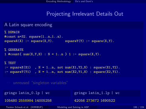
Encoding Methodology Do’s and Dont’s
Projecting Irrelevant Details Out
A Latin square encoding
% DOMAIN
#const n=32. square(1..n,1..n).
squareX(X) :- square(X,Y). squareY(Y) :- square(X,Y).
% GENERATE
1 #count{ num(X,Y,N) : N = 1..n } 1 :- square(X,Y).
% TEST
:- squareX(X1) , N = 1..n, not num(X1,Y2,N) : square(X1,Y2).
:- squareY(Y1) , N = 1..n, not num(X2,Y1,N) : square(X2,Y1).
+ unreused “singleton variables”
gringo latin_0.lp | wc
105480 2558984 14005258
gringo latin_1.lp | wc
42056 273672 1690522
Torsten Schaub et al. (KRR@UP) Modeling and Solving in ASP 195 / 226

Encoding Methodology Do’s and Dont’s
Unraveling Symmetric Inequalities
Another Latin square encoding
% DOMAIN
#const n=32. square(1..n,1..n).
% GENERATE
1 #count{ num(X,Y,N) : N = 1..n } 1 :- square(X,Y).
% TEST
:- num(X1,Y1,N), num(X1,Y2,N), Y1 != Y2.
:- num(X1,Y1,N), num(X2,Y1,N), X1 != X2.
+ duplicate ground rules (swapping Y1/Y2 and X1/X2 gives the “same”)
gringo latin_2.lp | wc
2071560 12389384 40906946
gringo latin_3.lp | wc
1055752 6294536 21099558
Torsten Schaub et al. (KRR@UP) Modeling and Solving in ASP 196 / 226

Encoding Methodology Do’s and Dont’s
Unraveling Symmetric Inequalities
Another Latin square encoding
% DOMAIN
#const n=32. square(1..n,1..n).
% GENERATE
1 #count{ num(X,Y,N) : N = 1..n } 1 :- square(X,Y).
% TEST
:- num(X1,Y1,N), num(X1,Y2,N), Y1 < Y2.
:- num(X1,Y1,N), num(X2,Y1,N), X1 < X2.
+ duplicate ground rules (swapping Y1/Y2 and X1/X2 gives the “same”)
gringo latin_2.lp | wc
2071560 12389384 40906946
gringo latin_3.lp | wc
1055752 6294536 21099558
Torsten Schaub et al. (KRR@UP) Modeling and Solving in ASP 196 / 226

Encoding Methodology Do’s and Dont’s
Linearizing Existence Tests
Still another Latin square encoding
% DOMAIN
#const n=32. square(1..n,1..n).
% GENERATE
1 #count{ num(X,Y,N) : N = 1..n } 1 :- square(X,Y).
% TEST
:- num(X1,Y1,N), num(X1,Y2,N), Y1 < Y2.
:- num(X1,Y1,N), num(X2,Y1,N), X1 < X2.
+ uniqueness of N in a row/column checked by ENUMERATING PAIRS!
gringo latin_3.lp | wc
1055752 6294536 21099558
gringo latin_4.lp | wc
228360 1205256 4780744
Torsten Schaub et al. (KRR@UP) Modeling and Solving in ASP 197 / 226

Encoding Methodology Do’s and Dont’s
Linearizing Existence Tests
Still another Latin square encoding
% DOMAIN
#const n=32. square(1..n,1..n).
% GENERATE
1 #count{ num(X,Y,N) : N = 1..n } 1 :- square(X,Y).
% DEFINE + TEST
gtX(X-1,Y,N) :- num(X,Y,N), 1 < X. gtY(X,Y-1,N) :- num(X,Y,N), 1 < Y.
gtX(X-1,Y,N) :- gtX(X,Y,N), 1 < X. gtY(X,Y-1,N) :- gtY(X,Y,N), 1 < Y.
:- num(X,Y,N), gtX(X,Y,N). :- num(X,Y,N), gtY(X,Y,N).
+ uniqueness of N in a row/column checked by ENUMERATING PAIRS!
gringo latin_3.lp | wc
1055752 6294536 21099558
gringo latin_4.lp | wc
228360 1205256 4780744
Torsten Schaub et al. (KRR@UP) Modeling and Solving in ASP 197 / 226

Encoding Methodology Do’s and Dont’s
Assigning Aggregate Values
Yet another Latin square encoding
% DOMAIN
#const n=32. square(1..n,1..n).
sigma(S) :- S = #sum[ square(X,n) = X ].
% GENERATE
1 #count{ num(X,Y,N) : N = 1..n } 1 :- square(X,Y).
% DEFINE + TEST
occX(X,N,C) :- X = 1..n, N = 1..n, C = #count{ num(X,Y,N) }.
occY(Y,N,C) :- Y = 1..n, N = 1..n, C = #count{ num(X,Y,N) }.
:- occX(X,N,C), C != 1. :- occY(Y,N,C), C != 1.
% DISPLAY
#hide. #show num/3. #show sigma/1.
gringo latin_5.lp | wc
304136 5778440 30252505
gringo latin_6.lp | wc
48136 373768 2185042Torsten Schaub et al. (KRR@UP) Modeling and Solving in ASP 198 / 226
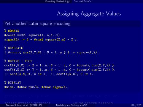

Encoding Methodology Do’s and Dont’s
Assigning Aggregate Values
Yet another Latin square encoding
% DOMAIN
#const n=32. square(1..n,1..n).
sigma(S) :- S = #sum[ square(X,n) = X ]. 4
% GENERATE
1 #count{ num(X,Y,N) : N = 1..n } 1 :- square(X,Y).
% DEFINE + TEST
occX(X,N,C) :- X = 1..n, N = 1..n, C = #count{ num(X,Y,N) }.
occY(Y,N,C) :- Y = 1..n, N = 1..n, C = #count{ num(X,Y,N) }.
:- occX(X,N,C), C != 1. :- occY(Y,N,C), C != 1.
% DISPLAY
#hide. #show num/3. #show sigma/1.
gringo latin_5.lp | wc
304136 5778440 30252505
gringo latin_6.lp | wc
48136 373768 2185042Torsten Schaub et al. (KRR@UP) Modeling and Solving in ASP 198 / 226

Encoding Methodology Do’s and Dont’s
Assigning Aggregate Values
Yet another Latin square encoding
% DOMAIN
#const n=32. square(1..n,1..n).
sigma(S) :- S = #sum[ square(X,n) = X ].
% GENERATE
1 #count{ num(X,Y,N) : N = 1..n } 1 :- square(X,Y).
% DEFINE + TEST
occX(X,N,C) :- X = 1..n, N = 1..n, C = #count{ num(X,Y,N) }.
occY(Y,N,C) :- Y = 1..n, N = 1..n, C = #count{ num(X,Y,N) }.
:- occX(X,N,C), C != 1. :- occY(Y,N,C), C != 1.
% DISPLAY
#hide. #show num/3. #show sigma/1.
gringo latin_5.lp | wc
304136 5778440 30252505
gringo latin_6.lp | wc
48136 373768 2185042Torsten Schaub et al. (KRR@UP) Modeling and Solving in ASP 198 / 226

Encoding Methodology Do’s and Dont’s
Assigning Aggregate Values
Yet another Latin square encoding
% DOMAIN
#const n=32. square(1..n,1..n).
sigma(S) :- S = #sum[ square(X,n) = X ].
% GENERATE
1 #count{ num(X,Y,N) : N = 1..n } 1 :- square(X,Y).
% DEFINE + TEST
occX(X,N,C) :- X = 1..n, N = 1..n, C #count{ num(X,Y,N) } C, C = 0..n.
occY(Y,N,C) :- Y = 1..n, N = 1..n, C #count{ num(X,Y,N) } C, C = 0..n.
:- occX(X,N,C), C != 1. :- occY(Y,N,C), C != 1.
% DISPLAY
#hide. #show num/3. #show sigma/1.
+ internal transformation by gringo
Torsten Schaub et al. (KRR@UP) Modeling and Solving in ASP 198 / 226

Encoding Methodology Do’s and Dont’s
Assigning Aggregate Values
Yet another Latin square encoding
% DOMAIN
#const n=32. square(1..n,1..n).
sigma(S) :- S = #sum[ square(X,n) = X ].
% GENERATE
1 #count{ num(X,Y,N) : N = 1..n } 1 :- square(X,Y).
% DEFINE + TEST
occX(X,N,C) :- X = 1..n, N = 1..n, C = #count{ num(X,Y,N) }. 7
occY(Y,N,C) :- Y = 1..n, N = 1..n, C = #count{ num(X,Y,N) }. 7
:- occX(X,N,C), C != 1. :- occY(Y,N,C), C != 1.
% DISPLAY
#hide. #show num/3. #show sigma/1.
gringo latin_5.lp | wc
304136 5778440 30252505
gringo latin_6.lp | wc
48136 373768 2185042Torsten Schaub et al. (KRR@UP) Modeling and Solving in ASP 198 / 226

Encoding Methodology Do’s and Dont’s
Assigning Aggregate Values
Yet another Latin square encoding
% DOMAIN
#const n=32. square(1..n,1..n).
% GENERATE
1 #count{ num(X,Y,N) : N = 1..n } 1 :- square(X,Y).
% DEFINE + TEST
occX(X,N,C) :- X = 1..n, N = 1..n, C = #count{ num(X,Y,N) }.
occY(Y,N,C) :- Y = 1..n, N = 1..n, C = #count{ num(X,Y,N) }.
:- occX(X,N,C), C != 1. :- occY(Y,N,C), C != 1.
% DISPLAY
#hide. #show num/3.
gringo latin_5.lp | wc gringo latin_6.lp | wc
48136 373768 2185042
Torsten Schaub et al. (KRR@UP) Modeling and Solving in ASP 198 / 226

Encoding Methodology Do’s and Dont’s
Assigning Aggregate Values
Yet another Latin square encoding
% DOMAIN
#const n=32. square(1..n,1..n).
% GENERATE
1 #count{ num(X,Y,N) : N = 1..n } 1 :- square(X,Y).
% DEFINE + TEST
occX(X,N,C) :- X = 1..n, N = 1..n, C = #count{ num(X,Y,N) }.
occY(Y,N,C) :- Y = 1..n, N = 1..n, C = #count{ num(X,Y,N) }.
:- occX(X,N,C), C != 1. :- occY(Y,N,C), C != 1.
% DISPLAY
#hide. #show num/3.
gringo latin_5.lp | wc
304136 5778440 30252505
gringo latin_6.lp | wc
48136 373768 2185042
Torsten Schaub et al. (KRR@UP) Modeling and Solving in ASP 198 / 226

Encoding Methodology Do’s and Dont’s
Assigning Aggregate Values
Yet another Latin square encoding
% DOMAIN
#const n=32. square(1..n,1..n).
% GENERATE
1 #count{ num(X,Y,N) : N = 1..n } 1 :- square(X,Y).
% TEST
:- X = 1..n, N = 1..n, not 1 #count{ num(X,Y,N) } 1.
:- Y = 1..n, N = 1..n, not 1 #count{ num(X,Y,N) } 1.
% DISPLAY
#hide. #show num/3.
gringo latin_5.lp | wc
304136 5778440 30252505
gringo latin_6.lp | wc
48136 373768 2185042
Torsten Schaub et al. (KRR@UP) Modeling and Solving in ASP 198 / 226

Encoding Methodology Do’s and Dont’s
Breaking Symmetries
The ultimate Latin square encoding?
% DOMAIN
#const n=32. square(1..n,1..n).
% GENERATE
1 #count{ num(X,Y,N) : N = 1..n } 1 :- square(X,Y).
% TEST
:- X = 1..n, N = 1..n, not 1 #count{ num(X,Y,N) } 1.
:- Y = 1..n, N = 1..n, not 1 #count{ num(X,Y,N) } 1.
% DISPLAY
#hide. #show num/3.
Torsten Schaub et al. (KRR@UP) Modeling and Solving in ASP 199 / 226

Encoding Methodology Do’s and Dont’s
Breaking Symmetries
The ultimate Latin square encoding?
% DOMAIN
#const n=32. square(1..n,1..n).
% GENERATE
1 #count{ num(X,Y,N) : N = 1..n } 1 :- square(X,Y).
% TEST
:- X = 1..n, N = 1..n, not 1 #count{ num(X,Y,N) } 1.
:- Y = 1..n, N = 1..n, not 1 #count{ num(X,Y,N) } 1.
% DISPLAY
#hide. #show num/3.
+ many symmetric solutions (mirroring, rotation, value permutation)
Torsten Schaub et al. (KRR@UP) Modeling and Solving in ASP 199 / 226

Encoding Methodology Do’s and Dont’s
Breaking Symmetries
The ultimate Latin square encoding?
% DOMAIN
#const n=32. square(1..n,1..n).
% GENERATE
1 #count{ num(X,Y,N) : N = 1..n } 1 :- square(X,Y).
% TEST
:- X = 1..n, N = 1..n, not 1 #count{ num(X,Y,N) } 1.
:- Y = 1..n, N = 1..n, not 1 #count{ num(X,Y,N) } 1.
% DISPLAY
#hide. #show num/3.
+ easy and safe to fix a full row/column!
Torsten Schaub et al. (KRR@UP) Modeling and Solving in ASP 199 / 226

Encoding Methodology Do’s and Dont’s
Breaking Symmetries
The ultimate Latin square encoding?
% DOMAIN
#const n=32. square(1..n,1..n).
% GENERATE
1 #count{ num(X,Y,N) : N = 1..n } 1 :- square(X,Y).
% TEST
:- X = 1..n, N = 1..n, not 1 #count{ num(X,Y,N) } 1.
:- Y = 1..n, N = 1..n, not 1 #count{ num(X,Y,N) } 1.
:- square(1,Y), not num(1,Y,Y). % Symmetry Breaking
% DISPLAY
#hide. #show num/3.
+ Let’s compare enumeration speed!
Torsten Schaub et al. (KRR@UP) Modeling and Solving in ASP 199 / 226

Encoding Methodology Do’s and Dont’s
Breaking Symmetries
The ultimate Latin square encoding?
% DOMAIN
#const n=32. square(1..n,1..n).
% GENERATE
1 #count{ num(X,Y,N) : N = 1..n } 1 :- square(X,Y).
% TEST
:- X = 1..n, N = 1..n, not 1 #count{ num(X,Y,N) } 1.
:- Y = 1..n, N = 1..n, not 1 #count{ num(X,Y,N) } 1.
% DISPLAY
#hide. #show num/3.
gringo -c n=5 latin_6.lp | clasp -q 0
Models : 161280 Time : 2.078s
Torsten Schaub et al. (KRR@UP) Modeling and Solving in ASP 199 / 226

Encoding Methodology Do’s and Dont’s
Breaking Symmetries
The ultimate Latin square encoding?
% DOMAIN
#const n=32. square(1..n,1..n).
% GENERATE
1 #count{ num(X,Y,N) : N = 1..n } 1 :- square(X,Y).
% TEST
:- X = 1..n, N = 1..n, not 1 #count{ num(X,Y,N) } 1.
:- Y = 1..n, N = 1..n, not 1 #count{ num(X,Y,N) } 1.
:- square(1,Y), not num(1,Y,Y). % Symmetry Breaking
% DISPLAY
#hide. #show num/3.
gringo -c n=5 latin_7.lp | clasp -q 0
Models : 1344 Time : 0.024s
Torsten Schaub et al. (KRR@UP) Modeling and Solving in ASP 199 / 226

Hints
Effective Modeling: Overview
28 Problems as Logic Programs (Revisited)Graph ColoringHamiltonian CycleTraveling Salesperson
29 Encoding MethodologyTweaking N-QueensDo’s and Dont’s
30 Hints
Torsten Schaub et al. (KRR@UP) Modeling and Solving in ASP 200 / 226

Hints
Encode With Care!
1 Create a working encoding
Q1: Do you need to modify the encoding if the facts change?Q2: Are all variables significant (or statically functionally dependent)?Q3: Can there be (many) identic ground rules?Q4: Do you enumerate pairs of values (to test uniqueness)?Q5: Do you assign dynamic aggregate values (to check a fixed bound)?Q6: Do you admit (obvious) symmetric solutions?Q7: Do you have additional domain knowledge simplifying the problem?Q8: Are you aware of anything else that, if encoded, would reduce
grounding and/or solving efforts?
2 Revise until no “Yes” answer!
+ If the format of facts makes encoding painful (for instance, abusinggrounding for “scientific calculations”), revise the fact format as well.
Torsten Schaub et al. (KRR@UP) Modeling and Solving in ASP 201 / 226

Hints
Some Hints on (Preventing) Debugging
Kinds of errors
syntactic . . . follow error messages by the grounder
semantic . . . (most likely) encoding/intention mismatch
Ways to identify semantic errors (early)
1 develop and test incrementally
prepare toy instances with “interesting features”build the encoding bottom-up and verify additions (eg. new predicates)
2 compare the encoded to the intended meaning
check whether the grounding fits (use gringo -t)if answer sets are unintended, investigate conditions that fail to holdif answer sets are missing, examine integrity constraints (add heads)
3 ask tools (eg. http://www.kr.tuwien.ac.at/research/projects/mmdasp/)
Torsten Schaub et al. (KRR@UP) Modeling and Solving in ASP 202 / 226

Hints
Overcoming Performance Bottlenecks
Grounding
monitor time spent by and output size of gringo
1 system tools (eg. time(gringo [. . . ] | wc))2 profiling info (eg. gringo --gstats --verbose=3 [. . . ] > /dev/null)
+ once identified, reformulate “critical” logic program parts
Solving
check solving statistics (use clasp --stats)
+ if great search efforts (Conflicts/Choices/Restarts), then
1 try auto-configuration (offered by claspfolio)2 try manual fine-tuning (requires expert knowledge!)3 if possible, reformulate the problem or add domain knowledge
(“redundant” constraints) to help the solver
Torsten Schaub et al. (KRR@UP) Modeling and Solving in ASP 203 / 226

Systems: Overview
31 Potassco
32 gringo
33 clasp
34 Siblingsclaspfolioclingconiclingooclingo
35 Book
Torsten Schaub et al. (KRR@UP) Modeling and Solving in ASP 204 / 226

Potassco
Systems: Overview
31 Potassco
32 gringo
33 clasp
34 Siblingsclaspfolioclingconiclingooclingo
35 Book
Torsten Schaub et al. (KRR@UP) Modeling and Solving in ASP 205 / 226

Potassco
http://potassco.sourceforge.net
Potassco, the Potsdam Answer Set Solving Collection,bundles tools for ASP developed at the University of Potsdam,for instance:
Grounder: gringo, pyngo
Solver: clasp, claspd, claspar
Grounder+Solver: clingo, iclingo, oclingo, clingcon
Further Tools: claspfolio, coala, inca, plasp, sbass, xorro
Benchmark repository: http://asparagus.cs.uni-potsdam.de
Torsten Schaub et al. (KRR@UP) Modeling and Solving in ASP 206 / 226

gringo
Systems: Overview
31 Potassco
32 gringo
33 clasp
34 Siblingsclaspfolioclingconiclingooclingo
35 Book
Torsten Schaub et al. (KRR@UP) Modeling and Solving in ASP 207 / 226

gringo
gringo
Accepts safe programs with aggregates
Tolerates unrestricted use of function symbols(as long as it yields a finite ground instantiation :)
Expressive power of a Turing machine
Basic architecture of gringo:
Parser Preprocessor Grounder Output
--lparse--text--reify
--ground
Torsten Schaub et al. (KRR@UP) Modeling and Solving in ASP 208 / 226

clasp
Systems: Overview
31 Potassco
32 gringo
33 clasp
34 Siblingsclaspfolioclingconiclingooclingo
35 Book
Torsten Schaub et al. (KRR@UP) Modeling and Solving in ASP 209 / 226

clasp
clasp
Native ASP solver combining conflict-driven search withsophisticated reasoning techniques:
Advanced preprocessing including, e.g., equivalence reasoningLookback-based decision heuristicsRestart policiesNogood deletionProgress savingDedicated data structures for binary and ternary nogoodsLazy data structures (watched literals) for long nogoodsDedicated data structures for cardinality and weight constraintsLazy unfounded set checking based on “source pointers”Tight integration of unit propagation and unfounded set checkingReasoning modesMulti-threaded search. . .
Torsten Schaub et al. (KRR@UP) Modeling and Solving in ASP 210 / 226

clasp
Reasoning modes of clasp
Beyond deciding answer set existence, clasp allows for:
Optimization
Enumeration [without solution recording]
Projective Enumeration [without solution recording]
Brave and Cautious Reasoning determining the
union orintersection
of all answer sets by computing only linearly many of them
and combinations thereof
clasp also allows for solving
propositional CNF formulas (extended dimacs)
pseudo-Boolean formulas (opb and wbo)
Torsten Schaub et al. (KRR@UP) Modeling and Solving in ASP 211 / 226

clasp
Multi-threaded architecture of clasp
Solver 1. . . n
DecisionHeuristicDecisionHeuristic
ConflictResolution
ConflictResolution
AssignmentAtoms/Bodies
Recorded Nogoods
Propagation
UnitPropagation
UnitPropagation
PostPropagation
PostPropagation
PostPropagation
PostPropagation
Coordination
SharedContext
PropositionalVariables
Atoms Bodies
Static Nogoods
Implication Graph
ParallelContext
Threads S1 S2. . . Sn
Counter T W . . . S
Queue P1 P2. . . Pn
Shared Nogoods
EnumeratorEnumerator
NogoodDistributor
NogoodDistributor
LogicProgram
Preprocessing
ProgramBuilder
ProgramBuilder
PreprocessorPreprocessorPreprocessorPreprocessor
Torsten Schaub et al. (KRR@UP) Modeling and Solving in ASP 212 / 226
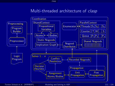

Siblings
Systems: Overview
31 Potassco
32 gringo
33 clasp
34 Siblingsclaspfolioclingconiclingooclingo
35 Book
Torsten Schaub et al. (KRR@UP) Modeling and Solving in ASP 213 / 226

Siblings claspfolio
claspfolio
Automatic selection of clasp configurationamong 22 configuration via (learned) classifiers
Basic architecture of claspfolio:
gringo clasp Prediction clasp
Models claspfolio
Torsten Schaub et al. (KRR@UP) Modeling and Solving in ASP 214 / 226

Siblings clingcon
clingcon
Hybrid grounding and solving
Solving in hybrid domains, like Bio-Informatics
Basic architecture of clingcon:
TheoryLanguage
gringo clasp
TheoryPropagator
TheorySolver
clingcon
Torsten Schaub et al. (KRR@UP) Modeling and Solving in ASP 215 / 226

Siblings clingcon
Pouring Water into Buckets on a Scale
time(0..t). $domain(0..500).
bucket(a). volume(a,0) $== 0.
bucket(b). volume(b,0) $== 100.
1 { pour(B,T) : bucket(B) } 1 :- time(T), T < t.
1 $<= amount(B,T) :- pour(B,T), T < t.
amount(B,T) $<= 30 :- pour(B,T), T < t.
amount(B,T) $== 0 :- not pour(B,T), bucket(B), time(T), T < t.
volume(B,T+1) $== volume(B,T) + amount(B,T) :- bucket(B), time(T), T < t.
down(B,T) :- volume(C,T) $< volume(B,T), bucket(B;C), time(T).
up(B,T) :- not down(B,T), bucket(B), time(T).
:- up(a,t).
Torsten Schaub et al. (KRR@UP) Modeling and Solving in ASP 216 / 226

Siblings iclingo
iclingo
Incremental grounding and solving
Offline solving in dynamic domains, like Automated Planning
Basic architecture of iclingo:
gringo clasp
iclingo
Torsten Schaub et al. (KRR@UP) Modeling and Solving in ASP 217 / 226

Siblings iclingo
Incremental ASP Solving Process
LogicProgram Grounder Solver
AnswerSets
- - -
6����Modeling
Qk
Pk
B
GrounderQk
Pk
B
Q1
P1
B
8?
P2
Q2
8P3
Q3
8...
Pn
Qn
4
Torsten Schaub et al. (KRR@UP) Modeling and Solving in ASP 218 / 226

Siblings iclingo
Incremental ASP Solving Process
LogicProgram Grounder Solver
AnswerSets
- - -
6����Modeling
Qk
Pk
B
GrounderQk
Pk
B
Q1
P1
B
8?
P2
Q2
8P3
Q3
8...
Pn
Qn
4
Torsten Schaub et al. (KRR@UP) Modeling and Solving in ASP 218 / 226

Siblings iclingo
Incremental ASP Solving Process
LogicProgram
Grounder SolverAnswer
Sets- - -
6����Modeling
Qk
Pk
B
GrounderQk
Pk
B
Q1
P1
B
8?
P2
Q2
8P3
Q3
8...
Pn
Qn
4
Torsten Schaub et al. (KRR@UP) Modeling and Solving in ASP 218 / 226

Siblings iclingo
Incremental ASP Solving Process
LogicProgram
Grounder SolverAnswer
Sets- - -
6����Modeling
Qk
Pk
B
GrounderQk
Pk
B
Q1
P1
B
8?
P2
Q2
8P3
Q3
8...
Pn
Qn
4
Torsten Schaub et al. (KRR@UP) Modeling and Solving in ASP 218 / 226

Siblings iclingo
Incremental ASP Solving Process
LogicProgram Grounder
SolverAnswer
Sets
- -
-
6����Modeling
Qk
Pk
B
GrounderQk
Pk
B
Q1
P1
B
8?
P2
Q2
8P3
Q3
8...
Pn
Qn
4
Torsten Schaub et al. (KRR@UP) Modeling and Solving in ASP 218 / 226

Siblings iclingo
Incremental ASP Solving Process
LogicProgram Grounder
SolverAnswer
Sets
- -
-
6����Modeling
Qk
Pk
B
Grounder
Qk
Pk
B
Q1
P1
B
8?
P2
Q2
8P3
Q3
8...
Pn
Qn
4
Torsten Schaub et al. (KRR@UP) Modeling and Solving in ASP 218 / 226

Siblings iclingo
Incremental ASP Solving Process
LogicProgram Grounder
SolverAnswer
Sets
- -
-
6����Modeling
Qk
Pk
B
Grounder
Qk
Pk
B
Q1
P1
B
8
?
P2
Q2
8P3
Q3
8...
Pn
Qn
4
Torsten Schaub et al. (KRR@UP) Modeling and Solving in ASP 218 / 226

Siblings iclingo
Incremental ASP Solving Process
LogicProgram Grounder
SolverAnswer
Sets
- -
-
6����Modeling
Qk
Pk
B
Grounder
Qk
Pk
B
Q1
P1
B
8
?
P2
Q2
8P3
Q3
8...
Pn
Qn
4
Torsten Schaub et al. (KRR@UP) Modeling and Solving in ASP 218 / 226

Siblings iclingo
Incremental ASP Solving Process
LogicProgram Grounder
SolverAnswer
Sets
- -
-
6����Modeling
Qk
Pk
B
Grounder
Qk
Pk
B
Q1
P1
B
8
?
P2
Q2
8
P3
Q3
8...
Pn
Qn
4
Torsten Schaub et al. (KRR@UP) Modeling and Solving in ASP 218 / 226

Siblings iclingo
Incremental ASP Solving Process
LogicProgram Grounder
SolverAnswer
Sets
- -
-
6����Modeling
Qk
Pk
B
Grounder
Qk
Pk
B
Q1
P1
B
8
?
P2
Q2
8
P3
Q3
8
...Pn
Qn
4
Torsten Schaub et al. (KRR@UP) Modeling and Solving in ASP 218 / 226

Siblings iclingo
Incremental ASP Solving Process
LogicProgram Grounder
SolverAnswer
Sets
- -
-
6����Modeling
Qk
Pk
B
Grounder
Qk
Pk
B
Q1
P1
B
8
?
P2
Q2
8
P3
Q3
8
...Pn
Qn
4
Torsten Schaub et al. (KRR@UP) Modeling and Solving in ASP 218 / 226

Siblings iclingo
Simplistic STRIPS Planning
#base.
fluent(p). fluent(q). fluent(r).
action(a). pre(a,p). add(a,q). del(a,p).
action(b). pre(b,q). add(b,r). del(b,q).
init(p). query(r).
holds(P,0) :- init(P).
#cumulative t.
1 { occ(A,t) : action(A) } 1.
:- occ(A,t), pre(A,F), not holds(F,t-1).
ocdel(F,t) :- occ(A,t), del(A,F).
holds(F,t) :- occ(A,t), add(A,F).
holds(F,t) :- holds(F,t-1), not ocdel(F,t).
#volatile t.
:- query(F), not holds(F,t).
Torsten Schaub et al. (KRR@UP) Modeling and Solving in ASP 219 / 226

Siblings oclingo
oclingo
Reactive grounding and solving
Online solving in dynamic domains, like Robotics
Basic architecture of oclingo:
gringo clasp
oclingo
Controller
Torsten Schaub et al. (KRR@UP) Modeling and Solving in ASP 220 / 226

Siblings oclingo
Reactive ASP Solving Process
LogicProgram Grounder Solver
AnswerSets
- - -
6����Modeling
Qk
Pk
B
GrounderQk
Pk
B
6
E1
F1
E1
F1
BP1
...Pn1
Qn1
4
E2
F2
E1
F1
E2
F2
Pn2
Qn2
4
E3
F3
E2
F2
E1
F1
E3
F3
Pn3
Qn3
4Pn41
Qn41
E42
F42
E41
F41
E40
F40
E39
F39
E38
F38
E37
F37
E36
F36
E35
F35
E42...
F42
Pn42
Qn42
4
UpdateQueryErasure
8
Torsten Schaub et al. (KRR@UP) Modeling and Solving in ASP 221 / 226

Siblings oclingo
Reactive ASP Solving Process
LogicProgram
Grounder SolverAnswer
Sets- - -
6����Modeling
Qk
Pk
B
GrounderQk
Pk
B
6
E1
F1
E1
F1
BP1
...Pn1
Qn1
4
E2
F2
E1
F1
E2
F2
Pn2
Qn2
4
E3
F3
E2
F2
E1
F1
E3
F3
Pn3
Qn3
4Pn41
Qn41
E42
F42
E41
F41
E40
F40
E39
F39
E38
F38
E37
F37
E36
F36
E35
F35
E42...
F42
Pn42
Qn42
4
UpdateQueryErasure
8
Torsten Schaub et al. (KRR@UP) Modeling and Solving in ASP 221 / 226

Siblings oclingo
Reactive ASP Solving Process
LogicProgram Grounder
SolverAnswer
Sets
- -
-
6����Modeling
Qk
Pk
B
GrounderQk
Pk
B
6
E1
F1
E1
F1
B
P1...
Pn1
Qn1
4
E2
F2
E1
F1
E2
F2
Pn2
Qn2
4
E3
F3
E2
F2
E1
F1
E3
F3
Pn3
Qn3
4Pn41
Qn41
E42
F42
E41
F41
E40
F40
E39
F39
E38
F38
E37
F37
E36
F36
E35
F35
E42...
F42
Pn42
Qn42
4
UpdateQueryErasure
8
Torsten Schaub et al. (KRR@UP) Modeling and Solving in ASP 221 / 226

Siblings oclingo
Reactive ASP Solving Process
LogicProgram Grounder
SolverAnswer
Sets
- -
-
6����Modeling
Qk
Pk
B
Grounder
Qk
Pk
B
6
E1
F1
E1
F1
BP1
...Pn1
Qn1
4
E2
F2
E1
F1
E2
F2
Pn2
Qn2
4
E3
F3
E2
F2
E1
F1
E3
F3
Pn3
Qn3
4Pn41
Qn41
E42
F42
E41
F41
E40
F40
E39
F39
E38
F38
E37
F37
E36
F36
E35
F35
E42...
F42
Pn42
Qn42
4
UpdateQueryErasure
8
Torsten Schaub et al. (KRR@UP) Modeling and Solving in ASP 221 / 226

Siblings oclingo
Reactive ASP Solving Process
LogicProgram Grounder
SolverAnswer
Sets
- -
-
6����Modeling
Qk
Pk
B
Grounder
Qk
Pk
B
6
E1
F1
E1
F1
BP1
...
Pn1
Qn1
4
E2
F2
E1
F1
E2
F2
Pn2
Qn2
4
E3
F3
E2
F2
E1
F1
E3
F3
Pn3
Qn3
4Pn41
Qn41
E42
F42
E41
F41
E40
F40
E39
F39
E38
F38
E37
F37
E36
F36
E35
F35
E42...
F42
Pn42
Qn42
4
UpdateQueryErasure
8
Torsten Schaub et al. (KRR@UP) Modeling and Solving in ASP 221 / 226

Siblings oclingo
Reactive ASP Solving Process
LogicProgram Grounder
SolverAnswer
Sets
- -
-
6����Modeling
Qk
Pk
B
Grounder
Qk
Pk
B
6
E1
F1
E1
F1
BP1
...
Pn1
Qn1
4
E2
F2
E1
F1
E2
F2
Pn2
Qn2
4
E3
F3
E2
F2
E1
F1
E3
F3
Pn3
Qn3
4
Pn41
Qn41
E42
F42
E41
F41
E40
F40
E39
F39
E38
F38
E37
F37
E36
F36
E35
F35
E42...
F42
Pn42
Qn42
4
UpdateQueryErasure
8
Torsten Schaub et al. (KRR@UP) Modeling and Solving in ASP 221 / 226

Siblings oclingo
Reactive ASP Solving Process
LogicProgram Grounder
SolverAnswer
Sets
- -
-
6����Modeling
Qk
Pk
B
Grounder
Qk
Pk
B
6
E1
F1
E1
F1
BP1
...
Pn1
Qn1
4
E2
F2
E1
F1
E2
F2
Pn2
Qn2
4
E3
F3
E2
F2
E1
F1
E3
F3
Pn3
Qn3
4Pn41
Qn41
E42
F42
E41
F41
E40
F40
E39
F39
E38
F38
E37
F37
E36
F36
E35
F35
E42...
F42
Pn42
Qn42
4
UpdateQueryErasure
8
Torsten Schaub et al. (KRR@UP) Modeling and Solving in ASP 221 / 226

Siblings oclingo
Reactive ASP Solving Process
LogicProgram Grounder
SolverAnswer
Sets
- -
-
6����Modeling
Qk
Pk
B
Grounder
Qk
Pk
B
6
E1
F1
E1
F1
BP1
...
Pn1
Qn1
4
E2
F2
E1
F1
E2
F2
Pn2
Qn2
4
E3
F3
E2
F2
E1
F1
E3
F3
Pn3
Qn3
4Pn41
Qn41
E42
F42
E41
F41
E40
F40
E39
F39
E38
F38
E37
F37
E36
F36
E35
F35
E42...
F42
Pn42
Qn42
4
Update
QueryErasure
8
Torsten Schaub et al. (KRR@UP) Modeling and Solving in ASP 221 / 226

Siblings oclingo
Reactive ASP Solving Process
LogicProgram Grounder
SolverAnswer
Sets
- -
-
6����Modeling
Qk
Pk
B
Grounder
Qk
Pk
B
6
E1
F1
E1
F1
BP1
...
Pn1
Qn1
4
E2
F2
E1
F1
E2
F2
Pn2
Qn2
4
E3
F3
E2
F2
E1
F1
E3
F3
Pn3
Qn3
4Pn41
Qn41
E42
F42
E41
F41
E40
F40
E39
F39
E38
F38
E37
F37
E36
F36
E35
F35
E42...
F42
Pn42
Qn42
4
Update
Query
Erasure
8
Torsten Schaub et al. (KRR@UP) Modeling and Solving in ASP 221 / 226

Siblings oclingo
Reactive ASP Solving Process
LogicProgram Grounder
SolverAnswer
Sets
- -
-
6����Modeling
Qk
Pk
B
Grounder
Qk
Pk
B
6
E1
F1
E1
F1
BP1
...
Pn1
Qn1
4
E2
F2
E1
F1
E2
F2
Pn2
Qn2
4
E3
F3
E2
F2
E1
F1
E3
F3
Pn3
Qn3
4Pn41
Qn41
E42
F42
E41
F41
E40
F40
E39
F39
E38
F38
E37
F37
E36
F36
E35
F35
E42...
F42
Pn42
Qn42
4
UpdateQuery
Erasure
8
Torsten Schaub et al. (KRR@UP) Modeling and Solving in ASP 221 / 226

Siblings oclingo
Elevator Control
#base.
floor(1..3).
atFloor(1,0).
#cumulative t.
#external request(F,t) : floor(F).
1 { atFloor(F-1;F+1,t) } 1 :- atFloor(F,t-1), floor(F).
:- atFloor(F,t), not floor(F).
requested(F,t) :- request(F,t), floor(F), not atFloor(F,t).
requested(F,t) :- requested(F,t-1), floor(F), not atFloor(F,t).
goal(t) :- not requested(F,t) : floor(F).
#volatile t.
:- not goal(t).
Torsten Schaub et al. (KRR@UP) Modeling and Solving in ASP 222 / 226

Siblings oclingo
Pushing a button
oClingo acts as a server listening on a portwaiting for client requests
To issue such requests, a separate controller programsends online progressions using network sockets
For instance,
#step 1.
request(3,1).
#endstep.
This process terminates when the client sends
#stop.
Torsten Schaub et al. (KRR@UP) Modeling and Solving in ASP 223 / 226

Book
Systems: Overview
31 Potassco
32 gringo
33 clasp
34 Siblingsclaspfolioclingconiclingooclingo
35 Book
Torsten Schaub et al. (KRR@UP) Modeling and Solving in ASP 224 / 226

Book
The (forthcoming) Potassco Book
1. Motivation2. Introduction3. Basic modeling4. Grounding5. Characterizations6. Solving7. Systems8. Advanced modeling9. Conclusions
Answer Set Solving in Practice
Martin Gebser, Roland Kaminski, Benjamin Kaufmann, and Torsten SchaubUniversity of Potsdam
SYNTHESIS LECTURES ON SAMPLE SERIES #1
CM&
cLaypoolMorgan publishers&
http://potassco.sourceforge.net/teaching.html
Torsten Schaub et al. (KRR@UP) Modeling and Solving in ASP 225 / 226

Summary
ASP is emerging as a viable tool for Knowledge Representationand Reasoning
ASP offers efficient and versatile off-the-shelf solving technology
http://potassco.sourceforge.net
ASP’07/09/11, CASC’11, MISC’11, PB’09/11, and SAT’09/11
ASP offers an expanding functionality and ease of use
Rapid application development tool
ASP has a growing range of applications
ASP = KR+DB+SAT+LP
Torsten Schaub et al. (KRR@UP) Modeling and Solving in ASP 226 / 226

C. Anger, M. Gebser, T. Linke, A. Neumann, and T. Schaub.The nomore++ approach to answer set solving.In G. Sutcliffe and A. Voronkov, editors, Proceedings of the TwelfthInternational Conference on Logic for Programming, ArtificialIntelligence, and Reasoning (LPAR’05), volume 3835 of Lecture Notesin Artificial Intelligence, pages 95–109. Springer-Verlag, 2005.
Y. Babovich and V. Lifschitz.Computing answer sets using program completion.Unpublished draft; available athttp://www.cs.utexas.edu/users/tag/cmodels.html, 2003.
C. Baral.Knowledge Representation, Reasoning and Declarative ProblemSolving.Cambridge University Press, 2003.
C. Baral, G. Brewka, and J. Schlipf, editors.
Torsten Schaub et al. (KRR@UP) Modeling and Solving in ASP 226 / 226

Proceedings of the Ninth International Conference on LogicProgramming and Nonmonotonic Reasoning (LPNMR’07), volume4483 of Lecture Notes in Artificial Intelligence. Springer-Verlag, 2007.
S. Baselice, P. Bonatti, and M. Gelfond.Towards an integration of answer set and constraint solving.In M. Gabbrielli and G. Gupta, editors, Proceedings of the Twenty-firstInternational Conference on Logic Programming (ICLP’05), volume3668 of Lecture Notes in Computer Science, pages 52–66.Springer-Verlag, 2005.
A. Biere.Adaptive restart strategies for conflict driven SAT solvers.In H. Kleine Buning and X. Zhao, editors, Proceedings of the EleventhInternational Conference on Theory and Applications of SatisfiabilityTesting (SAT’08), volume 4996 of Lecture Notes in ComputerScience, pages 28–33. Springer-Verlag, 2008.
A. Biere.PicoSAT essentials.
Torsten Schaub et al. (KRR@UP) Modeling and Solving in ASP 226 / 226

Journal on Satisfiability, Boolean Modeling and Computation,4:75–97, 2008.
A. Biere, M. Heule, H. van Maaren, and T. Walsh, editors.Handbook of Satisfiability, volume 185 of Frontiers in ArtificialIntelligence and Applications.IOS Press, 2009.
M. Brain, O. Cliffe, and M. de Vos.A pragmatic programmer’s guide to answer set programming.In M. de Vos and T. Schaub, editors, Proceedings of the SecondWorkshop on Software Engineering for Answer Set Programming(SEA’09), volume 546, pages 49–63. CEUR Workshop Proceedings,2009.
M. Brain, M. Gebser, J. Puhrer, T. Schaub, H. Tompits, andS. Woltran.Debugging ASP programs by means of ASP.In Baral et al. , pages 31–43.
Torsten Schaub et al. (KRR@UP) Modeling and Solving in ASP 226 / 226

M. Brain, M. Gebser, J. Puhrer, T. Schaub, H. Tompits, andS. Woltran.That is illogical captain! — the debugging support tool spock foranswer-set programs: System description.In M. de Vos and T. Schaub, editors, Proceedings of the Workshop onSoftware Engineering for Answer Set Programming (SEA’07), volume281, pages 71–85. CEUR Workshop Proceedings, 2007.
K. Clark.Negation as failure.In H. Gallaire and J. Minker, editors, Logic and Data Bases, pages293–322. Plenum Press, 1978.
O. Cliffe, M. de Vos, M. Brain, and J. Padget.ASPVIZ: Declarative visualisation and animation using answer setprogramming.In Garcia de la Banda and Pontelli , pages 724–728.
M. D’Agostino, D. Gabbay, R. Hahnle, and J. Posegga, editors.Handbook of Tableau Methods.
Torsten Schaub et al. (KRR@UP) Modeling and Solving in ASP 226 / 226

Kluwer Academic Publishers, 1999.
E. Dantsin, T. Eiter, G. Gottlob, and A. Voronkov.Complexity and expressive power of logic programming.In Proceedings of the Twelfth Annual IEEE Conference onComputational Complexity (CCC’97), pages 82–101. IEEE ComputerSociety Press, 1997.
M. Davis, G. Logemann, and D. Loveland.A machine program for theorem-proving.Communications of the ACM, 5:394–397, 1962.
M. Davis and H. Putnam.A computing procedure for quantification theory.Journal of the ACM, 7:201–215, 1960.
C. Drescher, M. Gebser, T. Grote, B. Kaufmann, A. Konig,M. Ostrowski, and T. Schaub.Conflict-driven disjunctive answer set solving.
Torsten Schaub et al. (KRR@UP) Modeling and Solving in ASP 226 / 226

In G. Brewka and J. Lang, editors, Proceedings of the EleventhInternational Conference on Principles of Knowledge Representationand Reasoning (KR’08), pages 422–432. AAAI Press, 2008.
C. Drescher, M. Gebser, B. Kaufmann, and T. Schaub.Heuristics in conflict resolution.In M. Pagnucco and M. Thielscher, editors, Proceedings of theTwelfth International Workshop on Nonmonotonic Reasoning(NMR’08), number UNSW-CSE-TR-0819 in School of ComputerScience and Engineering, The University of New South Wales,Technical Report Series, pages 141–149, 2008.
N. Een and N. Sorensson.An extensible SAT-solver.In E. Giunchiglia and A. Tacchella, editors, Proceedings of the SixthInternational Conference on Theory and Applications of SatisfiabilityTesting (SAT’03), volume 2919 of Lecture Notes in ComputerScience, pages 502–518. Springer-Verlag, 2004.
T. Eiter and G. Gottlob.
Torsten Schaub et al. (KRR@UP) Modeling and Solving in ASP 226 / 226

On the computational cost of disjunctive logic programming:Propositional case.Annals of Mathematics and Artificial Intelligence, 15(3-4):289–323,1995.
F. Fages.Consistency of Clark’s completion and the existence of stable models.Journal of Methods of Logic in Computer Science, 1:51–60, 1994.
P. Ferraris.Answer sets for propositional theories.In C. Baral, G. Greco, N. Leone, and G. Terracina, editors, Proceedingsof the Eighth International Conference on Logic Programming andNonmonotonic Reasoning (LPNMR’05), volume 3662 of LectureNotes in Artificial Intelligence, pages 119–131. Springer-Verlag, 2005.
M. Fitting.A Kripke-Kleene semantics for logic programs.Journal of Logic Programming, 2(4):295–312, 1985.
M. Garcia de la Banda and E. Pontelli, editors.Torsten Schaub et al. (KRR@UP) Modeling and Solving in ASP 226 / 226

Proceedings of the Twenty-fourth International Conference on LogicProgramming (ICLP’08), volume 5366 of Lecture Notes in ComputerScience. Springer-Verlag, 2008.
M. Gebser, C. Guziolowski, M. Ivanchev, T. Schaub, A. Siegel,S. Thiele, and P. Veber.Repair and prediction (under inconsistency) in large biologicalnetworks with answer set programming.In F. Lin and U. Sattler, editors, Proceedings of the TwelfthInternational Conference on Principles of Knowledge Representationand Reasoning (KR’10), pages 497–507. AAAI Press, 2010.
M. Gebser, R. Kaminski, B. Kaufmann, M. Ostrowski, T. Schaub, andS. Thiele.A user’s guide to gringo, clasp, clingo, and iclingo.
M. Gebser, R. Kaminski, B. Kaufmann, M. Ostrowski, T. Schaub, andS. Thiele.Engineering an incremental ASP solver.In Garcia de la Banda and Pontelli , pages 190–205.
Torsten Schaub et al. (KRR@UP) Modeling and Solving in ASP 226 / 226

M. Gebser, R. Kaminski, B. Kaufmann, and T. Schaub.On the implementation of weight constraint rules in conflict-drivenASP solvers.In Hill and Warren , pages 250–264.
M. Gebser, R. Kaminski, B. Kaufmann, and T. Schaub.Multi-criteria optimization in answer set programming.In J. Gallagher and M. Gelfond, editors, Technical Communications ofthe Twenty-seventh International Conference on Logic Programming(ICLP’11), volume 11, pages 1–10. Leibniz International Proceedingsin Informatics (LIPIcs), 2011.
M. Gebser, R. Kaminski, B. Kaufmann, and T. Schaub.Multi-criteria optimization in ASP and its application to Linuxpackage configuration.Unpublished draft, 2011.Available athttp://www.cs.uni-potsdam.de/wv/pdfformat/gekakasc11b.pdf.
Torsten Schaub et al. (KRR@UP) Modeling and Solving in ASP 226 / 226

M. Gebser, R. Kaminski, B. Kaufmann, T. Schaub, M. Schneider, andS. Ziller.A portfolio solver for answer set programming: Preliminary report.In J. Delgrande and W. Faber, editors, Proceedings of the EleventhInternational Conference on Logic Programming and NonmonotonicReasoning (LPNMR’11), volume 6645 of Lecture Notes in ArtificialIntelligence, pages 352–357. Springer-Verlag, 2011.
M. Gebser, R. Kaminski, and T. Schaub.Complex optimization in answer set programming.Theory and Practice of Logic Programming, 11(4-5):821–839, 2011.
M. Gebser, B. Kaufmann, A. Neumann, and T. Schaub.clasp: A conflict-driven answer set solver.In Baral et al. , pages 260–265.
M. Gebser, B. Kaufmann, A. Neumann, and T. Schaub.Conflict-driven answer set enumeration.In Baral et al. , pages 136–148.
Torsten Schaub et al. (KRR@UP) Modeling and Solving in ASP 226 / 226

M. Gebser, B. Kaufmann, A. Neumann, and T. Schaub.Conflict-driven answer set solving.In Veloso , pages 386–392.
M. Gebser, B. Kaufmann, A. Neumann, and T. Schaub.Advanced preprocessing for answer set solving.In M. Ghallab, C. Spyropoulos, N. Fakotakis, and N. Avouris, editors,Proceedings of the Eighteenth European Conference on ArtificialIntelligence (ECAI’08), pages 15–19. IOS Press, 2008.
M. Gebser, B. Kaufmann, and T. Schaub.The conflict-driven answer set solver clasp: Progress report.In E. Erdem, F. Lin, and T. Schaub, editors, Proceedings of the TenthInternational Conference on Logic Programming and NonmonotonicReasoning (LPNMR’09), volume 5753 of Lecture Notes in ArtificialIntelligence, pages 509–514. Springer-Verlag, 2009.
M. Gebser, B. Kaufmann, and T. Schaub.Solution enumeration for projected Boolean search problems.
Torsten Schaub et al. (KRR@UP) Modeling and Solving in ASP 226 / 226

In W. van Hoeve and J. Hooker, editors, Proceedings of the SixthInternational Conference on Integration of AI and OR Techniques inConstraint Programming for Combinatorial Optimization Problems(CPAIOR’09), volume 5547 of Lecture Notes in Computer Science,pages 71–86. Springer-Verlag, 2009.
M. Gebser, M. Ostrowski, and T. Schaub.Constraint answer set solving.In Hill and Warren , pages 235–249.
M. Gebser, J. Puhrer, T. Schaub, and H. Tompits.A meta-programming technique for debugging answer-set programs.In D. Fox and C. Gomes, editors, Proceedings of the Twenty-thirdNational Conference on Artificial Intelligence (AAAI’08), pages448–453. AAAI Press, 2008.
M. Gebser and T. Schaub.Tableau calculi for answer set programming.In S. Etalle and M. Truszczynski, editors, Proceedings of theTwenty-second International Conference on Logic Programming
Torsten Schaub et al. (KRR@UP) Modeling and Solving in ASP 226 / 226

(ICLP’06), volume 4079 of Lecture Notes in Computer Science, pages11–25. Springer-Verlag, 2006.
M. Gebser and T. Schaub.Generic tableaux for answer set programming.In V. Dahl and I. Niemela, editors, Proceedings of the Twenty-thirdInternational Conference on Logic Programming (ICLP’07), volume4670 of Lecture Notes in Computer Science, pages 119–133.Springer-Verlag, 2007.
M. Gelfond.Answer sets.In V. Lifschitz, F. van Harmelen, and B. Porter, editors, Handbook ofKnowledge Representation, chapter 7, pages 285–316. ElsevierScience, 2008.
M. Gelfond and N. Leone.Logic programming and knowledge representation — the A-Prologperspective.Artificial Intelligence, 138(1-2):3–38, 2002.
Torsten Schaub et al. (KRR@UP) Modeling and Solving in ASP 226 / 226

M. Gelfond and V. Lifschitz.The stable model semantics for logic programming.In R. Kowalski and K. Bowen, editors, Proceedings of the FifthInternational Conference and Symposium of Logic Programming(ICLP’88), pages 1070–1080. MIT Press, 1988.
M. Gelfond and V. Lifschitz.Logic programs with classical negation.In Proceedings of the International Conference on Logic Programming,pages 579–597, 1990.
E. Giunchiglia, Y. Lierler, and M. Maratea.Answer set programming based on propositional satisfiability.Journal of Automated Reasoning, 36(4):345–377, 2006.
P. Hill and D. Warren, editors.Proceedings of the Twenty-fifth International Conference on LogicProgramming (ICLP’09), volume 5649 of Lecture Notes in ComputerScience. Springer-Verlag, 2009.
Torsten Schaub et al. (KRR@UP) Modeling and Solving in ASP 226 / 226

J. Huang.The effect of restarts on the efficiency of clause learning.In Veloso , pages 2318–2323.
H. Kautz and B. Selman.Planning as satisfiability.In B. Neumann, editor, Proceedings of the Tenth EuropeanConference on Artificial Intelligence (ECAI’92), pages 359–363. JohnWiley & sons, 1992.
K. Konczak, T. Linke, and T. Schaub.Graphs and colorings for answer set programming.Theory and Practice of Logic Programming, 6(1-2):61–106, 2006.
R. Kowalski.Logic for data description.In H. Gallaire and J. Minker, editors, Logic and Data Bases, pages77–103. Plenum Press, 1978.
J. Lee.
Torsten Schaub et al. (KRR@UP) Modeling and Solving in ASP 226 / 226

A model-theoretic counterpart of loop formulas.In L. Kaelbling and A. Saffiotti, editors, Proceedings of the NineteenthInternational Joint Conference on Artificial Intelligence (IJCAI’05),pages 503–508. Professional Book Center, 2005.
N. Leone, G. Pfeifer, W. Faber, T. Eiter, G. Gottlob, S. Perri, andF. Scarcello.The DLV system for knowledge representation and reasoning.ACM Transactions on Computational Logic, 7(3):499–562, 2006.
V. Lifschitz.Answer set programming and plan generation.Artificial Intelligence, 138(1-2):39–54, 2002.
V. Lifschitz and A. Razborov.Why are there so many loop formulas?ACM Transactions on Computational Logic, 7(2):261–268, 2006.
V. Lifschitz, L. Tang, and H. Turner.Nested expressions in logic programs.
Torsten Schaub et al. (KRR@UP) Modeling and Solving in ASP 226 / 226

Annals of Mathematics and Artificial Intelligence, 25(3-4):369–389,1999.
F. Lin and Y. Zhao.ASSAT: computing answer sets of a logic program by SAT solvers.Artificial Intelligence, 157(1-2):115–137, 2004.
J. Lloyd.Foundations of Logic Programming.Symbolic Computation. Springer-Verlag, 1987.
V. Marek and M. Truszczynski.Stable models and an alternative logic programming paradigm.In K. Apt, V. Marek, M. Truszczynski, and D. Warren, editors, TheLogic Programming Paradigm: a 25-Year Perspective, pages 375–398.Springer-Verlag, 1999.
J. Marques-Silva, I. Lynce, and S. Malik.Conflict-driven clause learning SAT solvers.In Biere et al. , chapter 4, pages 131–153.
Torsten Schaub et al. (KRR@UP) Modeling and Solving in ASP 226 / 226

J. Marques-Silva and K. Sakallah.GRASP: A search algorithm for propositional satisfiability.IEEE Transactions on Computers, 48(5):506–521, 1999.
V. Mellarkod and M. Gelfond.Integrating answer set reasoning with constraint solving techniques.In J. Garrigue and M. Hermenegildo, editors, Proceedings of the NinthInternational Symposium on Functional and Logic Programming(FLOPS’08), volume 4989 of Lecture Notes in Computer Science,pages 15–31. Springer-Verlag, 2008.
V. Mellarkod, M. Gelfond, and Y. Zhang.Integrating answer set programming and constraint logicprogramming.Annals of Mathematics and Artificial Intelligence, 53(1-4):251–287,2008.
D. Mitchell.A SAT solver primer.
Torsten Schaub et al. (KRR@UP) Modeling and Solving in ASP 226 / 226

Bulletin of the European Association for Theoretical ComputerScience, 85:112–133, 2005.
M. Moskewicz, C. Madigan, Y. Zhao, L. Zhang, and S. Malik.Chaff: Engineering an efficient SAT solver.In Proceedings of the Thirty-eighth Conference on Design Automation(DAC’01), pages 530–535. ACM Press, 2001.
I. Niemela.Logic programs with stable model semantics as a constraintprogramming paradigm.Annals of Mathematics and Artificial Intelligence, 25(3-4):241–273,1999.
R. Nieuwenhuis, A. Oliveras, and C. Tinelli.Solving SAT and SAT modulo theories: From an abstractDavis-Putnam-Logemann-Loveland procedure to DPLL(T).Journal of the ACM, 53(6):937–977, 2006.
J. Oetsch, J. Puhrer, and H. Tompits.
Torsten Schaub et al. (KRR@UP) Modeling and Solving in ASP 226 / 226

Catching the ouroboros: On debugging non-ground answer-setprograms.In Theory and Practice of Logic Programming. Twenty-sixthInternational Conference on Logic Programming (ICLP’10) SpecialIssue, volume 10(4-6), pages 513–529. Cambridge University Press,2010.
K. Pipatsrisawat and A. Darwiche.A lightweight component caching scheme for satisfiability solvers.In J. Marques-Silva and K. Sakallah, editors, Proceedings of the TenthInternational Conference on Theory and Applications of SatisfiabilityTesting (SAT’07), volume 4501 of Lecture Notes in ComputerScience, pages 294–299. Springer-Verlag, 2007.
L. Ryan.Efficient algorithms for clause-learning SAT solvers.Master’s thesis, Simon Fraser University, 2004.
J. Schlipf.The expressive powers of the logic programming semantics.
Torsten Schaub et al. (KRR@UP) Modeling and Solving in ASP 226 / 226

Journal of Computer and System Sciences, 51:64–86, 1995.
P. Simons, I. Niemela, and T. Soininen.Extending and implementing the stable model semantics.Artificial Intelligence, 138(1-2):181–234, 2002.
T. Syrjanen.Lparse 1.0 user’s manual.
A. van Gelder, K. Ross, and J. Schlipf.The well-founded semantics for general logic programs.Journal of the ACM, 38(3):620–650, 1991.
M. Veloso, editor.Proceedings of the Twentieth International Joint Conference onArtificial Intelligence (IJCAI’07). AAAI Press/The MIT Press, 2007.
L. Zhang, C. Madigan, M. Moskewicz, and S. Malik.Efficient conflict driven learning in a Boolean satisfiability solver.In Proceedings of the International Conference on Computer-AidedDesign (ICCAD’01), pages 279–285, 2001.
Torsten Schaub et al. (KRR@UP) Modeling and Solving in ASP 226 / 226