Modeling and Simulation with ODE (MSE)

Massimo Fornasier

Fakultat fur MathematikTechnische Universitat Munchenmassimo.fornasier@ma.tum.dehttp://www-m15.ma.tum.de/

Johann Radon Institute (RICAM)Osterreichische Akademie der Wissenschaften

massimo.fornasier@oeaw.ac.athttp://hdsparse.ricam.oeaw.ac.at/

Department of MathematicsTechnische Universitat Munchen

Lecture 1

Why are you here?In this course we shall provides the rudiments (the basics!) of thenumerical solution of differential equations, i.e, equations involvingthe derivatives of a (possibly) multivariate functionu : Ω ⊂ Rd → R:

F (x1, . . . , xd , u(x),∂

∂x1u(x), . . . ,

∂

∂xdu(x),

∂2

∂x1∂x1,

∂2

∂x1∂x2, . . . ,

∂2

∂x1∂xd, . . . ) = 0.

Often one of the variables indicates the time, e.g., x1 = t, and theequation governs a phenomena which evolves in time:

∂u

∂t+ F (x , u,Du,D2u, . . . ) = 0.

Differential equations were for thefirst time formulated in the 17th

century by I. Newton (1671) and byG.W. Leibniz (1676).

Just old boring stuff?

Yes, of course!?But also NO, because the history did not stop ...

used by Euler, Maxwell, Boltzmann, Navier, Stokes, Einstein,Prandtl, Schrodinger, Pauli, Dirac,Turing, Black&Scholes ...........

I provide an important modeling tool for the physical sciences,theoretical chemistry, biology, socio-economic sciences,engineering sciences ....

I accessible to numerical simulations

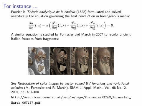
For instance ...Fourier in Theorie analytique de la chaleur (1822) formulated and solvedanalytically the equation governing the heat conduction in homogenous media:

∂u

∂t(t, x)− α

„∂2u

∂x21

(t, x) +∂2u

∂x22

(t, x) +∂2u

∂x23

(t, x)

«= 0.

A similar equation is studied by Fornasier and March in 2007 to recolor ancientItalian frescoes from fragments:

See Restoration of color images by vector valued BV functions and variationalcalculus (M. Fornasier and R. March), SIAM J. Appl. Math., Vol. 68 No. 2,2007, pp. 437-460.

http://www.ricam.oeaw.ac.at/people/page/fornasier/SIAM_Fornasier_

March_067187.pdf

Illustrations of differential equations and some of their(modern) applications

Reference: P. A. Markowich, Applied Partial Differential Equations - A Visual

Approach, Springer, 2006

Slides: http:

//homepage.univie.ac.at/peter.markowich/galleries/vortrag.pdf

I Gas dynamics Boltzmann equationI Fluid/gas dynamics: Navier-Stokes/Euler EquationsI Kinetic modeling of granular flowsI Chemotaxis and formation of biological patternsI Semiconductor modelingI Free boundary problems and interfacesI Reaction-diffusion equationsI Monge-Kantorovich optimal transportationI Wave equationsI Digital image processingI Socio-Economic modeling

From partial differential equations to ordinary differentialequations

As we shall see in the course of this lecture, several partialdifferential equations (PDE) can be reduced, after discretization ofthe space variable, to a system of ordinary differential equations(ODE):

∂u

∂t+ F (t, x , u,Du,D2u, . . . ) = 0⇒ u′h(t) + Fh(u(t)) = 0,

where h is a space discretization parameter.

The first part of this course is dedicated to the use of ODE formodeling physical and engineering problems, while the second partof the course is dedicated to their numerical solution by some ofthe most relevant numerical methods.

Program of the course in a nutshell

Modeling by ODE:

I First-order ODEs

I Second-order linear ODEs

I Higher-oder linear ODEs

I Systems of ODEs

Numerical methods for ODE:

I forward Euler method

I theta method

I Adams methods and more general multi-step methods

I Runge-Kutta methods

I stability and stiffness

I Backward differentiation formulae

References for this course

Besides the slides provided after the lecture online ...Books:

K11 E. Kreyszig, Advanced Engineering Mathematics, 10th Edition, JohnWiley & Sons, Inc., 2011

I09 A. Iserles, A First Course in the Numerical Analysis of DifferentialEquations (2nd ed.), Cambridge University Press, 2009.

QSG10 A. Quarteroni, F. Saleri, P. Gervasio, Scientific Computing with Matlaband Octave (3rd ed.), Springer, 2010.

Lecture notes:

F13 M. Fornasier, Numerik der gewohnlichen Differentialgleichungen,http://www-m3.ma.tum.de/foswiki/pub/M3/NumerikDG13/WebHome/

Numerik_2013-08-04.pdf (password required)

All you find at the webpage of the course:

http://www-m15.ma.tum.de/Allgemeines/ModelingSimulation

References do not mean ...

How does a book work? ...

References do not mean ...

that you do not come to the lecture and think to be smart ...

’cause I will NOT let you escape ...

At the end there will be the exam ... and I’ll be waiting for youthere (REMEMBER IT!) ...you better show up! (just a friendly - Italian - invitation not toskip the lectures :-) !)

Just the classical email from the “smart” student ...

Sehr geehrter Herr Prof. Fornasier,mein Name ist [SmartStudentName]. Gestern habe ich die Prufung in”Numerisches Programmieren II (CSE)” geschrieben. Ich habe extrem viel furdiese Prufung gelernt, da ich mich vor allem in PDEs spezialisieren mochte undim nachsten Semester auch “Numerik der PDEs” bei Prof.[ReallySmartProfName] horen werde. Mich zieht es innerhalb von CSE auchimmer mehr in Richtung Numerik und daher investiere ich viel Kraft in diesesThema. Ich habe mich mit wirklich allen Satzen, Beweisen und auch denThemen nach FEM (hyp./par. PDEs, die Sie nicht mehr behandelt haben) undauch daruber hinaus mit dem Buch von Iserles, “PDEs” von Lawrence Evansund weiterer Literatur beschaftigt und bin der Meinung, dass ich fur einenCSE-Studenten viel mehr Wissen als erforderlich besitze und vieleZusammenhange sehr gut verstanden habe.An dieser Stelle mochte ich meinen Unmut uber die gestrige Prufungausdrucken. Ich hatte bereits in NP1 eine 1.0 und dies war auch gestern meinZiel. Vermutlich habe ich nun gar nicht bestanden oder wenn, dann vielleichthochstens mit einer 4.0.[...]

Vielen herzlichen Dank.

Eh, eh, eh! He has NOT attended the lecture!

Let’s start ... why ODE?

As just mentioned, ODE comes often after the space discretizationof PDE.

But ODE have their own dignity and relevance, since, actually,PDE can be derived as the “limit” of sytems of ODE governing theevolution of particles driven by Newton laws:

F = m · a.

Hence, ODE ⇒ PDE ⇒ ODE.

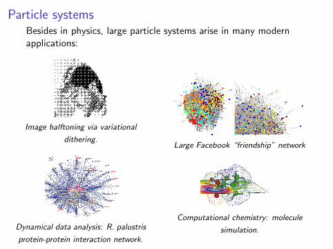
Particle systemsBesides in physics, large particle systems arise in many modernapplications:

Image halftoning via variational

dithering.

Dynamical data analysis: R. palustris

protein-protein interaction network.

Large Facebook “friendship” network

Computational chemistry: molecule

simulation.

Social dynamics

We consider large particle systems ofform:

xi = vi ,

vi =∑N

j=1 H(xj − xi , vj − vi ),

Several“social forces” encoded in theinteraction kernel H:

I Repulsion-attraction

I Alignment

I ...

Possible noise/uncertainty by addingstochastic terms.

Patterns related to different balance of

social forces.

Understanding how superposition of re-iterated binary “socialforces” yields global self-organization.

An example inspired by nature

Mills in nature and in our simulations.

J. A. Carrillo, M. Fornasier, G. Toscani, and F. Vecil, Particle, kinetic,

hydrodynamic models of swarming, within the book “Mathematical modeling

of collective behavior in socio-economic and life-sciences”, Birkhauser (Eds.

Lorenzo Pareschi, Giovanni Naldi, and Giuseppe Toscani), 2010.

http://www.ricam.oeaw.ac.at/people/page/fornasier/bookfinal.pdf

The genearal ODEOur goal is to use equations of the type

y ′ = f (t, y), t ≥ t0, y(t0) = y0, (1)

for modeling and then for simulation. (In the previous modeling,yi = (xi , vi ) and f (t, y)i = (vi ,

∑Nj=1 H(xj − xi , vj − vi )).)

I f is a map of [t0,∞)× Rd to Rd and the initial conditiony0 ∈ Rd is a given vector

I f is “nice”, obeying, in a given vector norm, the Lipschitzcondition

‖f (t, x)− f (t, y)‖ ≤ λ‖x − y‖, ∀x , y ∈ Rd , t ≥ t0 (2)

Here λ > 0 is a real constant that is independent of thechoice of x and y . In this case we say that f is a Lipschitzcontinuous function.

I Subject to (2), it is possible to prove that the ODE system(1) possesses a unique solution (see, for instance [Theorem3.5, F13] pag. 52).

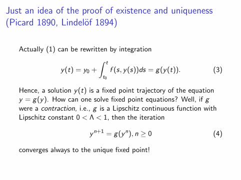
Just an idea of the proof of existence and uniqueness(Picard 1890, Lindelof 1894)

Actually (1) can be rewritten by integration

y(t) = y0 +

∫ t

t0

f (s, y(s))ds = g(y(t)). (3)

Hence, a solution y(t) is a fixed point trajectory of the equationy = g(y). How can one solve fixed point equations? Well, if gwere a contraction, i.e., g is a Lipschitz continuous function withLipschitz constant 0 < Λ < 1, then the iteration

yn+1 = g(yn), n ≥ 0 (4)

converges always to the unique fixed point!

Graphical interpretation and mathematical explanation

Indeed, assume that such fixed point y exists then

‖y−yn+1‖∗ = ‖g(y)−g(yn)‖∗ ≤ Λ‖y−yn‖∗ ≤ Λn‖y−y0‖∗ → 0, n→∞,

because Λ < 1. The tricky part of the proof is to show that thereexists a fixed point and that there exists always a norm ‖ · ‖∗ whichmakes g a contraction as soon as f is Lipschitz continuous.

Did you noticed that ...... what we wrote in (4) is actually an ALGORITHM?!

OMG! Really, an ALGORITHM?!

... is it a bad thing?!Actually, no, that’s what you are here for! Or, perhaps yes ... Ohwell, nevertheless, an ALGORITHM!

For the brave student: if you find out a way to discretize (4) and a way of

properly “scaling” the equation so that the iteration always converges on a

finite set of time point t0 < t1 < · < tn, then let me know! Actually this course

is (IMPLICITLY) all about this!

From Picard-Lindelof back to Euler: “greed is good!”Instead of solving globally the fixed point equation (3) by amultitude of iterations (4), we may consider the simpler idea ofsolving it locally, step by step, by iterating the approximation

y(t) = y0+

∫ t

t0

f (s, y(s))ds ≈ y(t0)+(t−t0)f (t0, y(t0)), for t ≈ t0.

(5)Given a sequence t0, t1 = t0 + h, t2 = t0 + 2h, ... , where h > 0 isa time step, we denote by yn a numerical estimate of the exactsolution y(tn), n = 0, 1, . . . . Motivated by (5), we choose

y1 = y0 + hf (t0, y0).

If h is small, it should not be that wrong! But then, why not tocontinue, assuming that we did not that bad before, at t2, t3 andso on. In general, we obtain the recursive scheme

yn+1 = yn + hf (tn, yn), (6)

the celebrated Euler method.

Graphical interpretationConsider the Euler method applied to the logistic equation

y ′ = y(1− y), y(0) =1

10,

with step h = 1:

It’s clear that at each step we produce an error, but our goal is not to avoid

any (numerical error)! (Eventually nobody is perfect!) Our final goal is to have

a practical method that approximates the analytic solution with increasing

accuracy (i.e., decreasing error) the more computational effort we do.

Yes, but what hell is this logistic equation? Is it justmathematical nonsense?!

The logistic equation is a model

OMG! Really, a MODEL?!

of population growth first published by Pierre Verhulst (1845,1847). Its solution is the function

y(t) =1

1 + e−t, t ∈ R.

Try it out and check that y ′(t) = y(t)(1− y(t)) (Exercise)!

Yes, but what hell is this logistic equation? Is it justmathematical nonsense?!

The logistic function finds applications in a range of fields, including artificialneural networks, biology, especially ecology, biomathematics, chemistry,demography, economics, geoscience, mathematical psychology, probability,sociology, political science, and statistics.In population dynamics one describes the growth of the population P(t) by

dP(t)

dt= rP(t)

„1− P(t)

K

«.

The term rP(t) on the right-hand side tells that for r > 0 the larger is thepopulation the stronger the growth will be (he, he, he) ... however the negativeterm − r

KP(t)2 instead indicates the drop of the population due to - interacting

- competition. This antagonistic effect is called the bottleneck, and is modeledby the value of the parameter K > 0. By setting y = P(t)

Kone obtains

y ′(t) = ry(t)(1− y(t)),

which for r = 1 is just our equation.

How to implement Euler’s method in MATLAB

Try out Euler’s method on the logistic equation:

f = @(t,x) x.*(1-x); [t,yy]=ode45(f,[0:5],1/10); y(1)=1/10;h=1; for n=1:5, y(n+1)=y(n)+h*y(n)*(1-y(n)); end,plot([0:5],y,’r*-’,[0:5],yy,’b’) h=1/2; for n=1:10,y(n+1)=y(n)+h*y(n)*(1-y(n)), end, hold on,plot([0:0.5:5],y,’g-*’)

Convergence of a numerical method

Assume that h > 0 is variable and h→ 0. On each grid t0,t1 = t0 + h, t2 = t0 + 2h, ... we associate a different numericalsequence yn = yn,h, n = 0, 1, . . . , bt∗/hc (not necessarily producedby the Euler method!).

A method is said to be convergent if, for every ODE (1) with aLipschitz function f and every t∗ > 0 it is true that

limh→0

maxn=0,1,...,bt∗/hc

‖yn,h − y(tn)‖ = 0,

where bαc ∈ Z is the integer part of α ∈ R.

Convergence means that, for every Lipschitz function,the numerical solution tends to the true solution as thegrid becomes increasingly fine.

Convergence of the Euler method

TheoremThe Euler method (6) is convergent

Proof. (For this proof we assume that the Taylor expansion of f has uniformlybounded coefficients, i.e., f is analytic, implying that y is analytic as well.) Letus consider the error en,h = yn − y(tn). We shall prove limh→0 ‖en,h‖ = 0.Taylor expansion of y(t)

y(tn+1) = y(tn) + hy ′(tn) +O(h2) = y(tn) + hf (tn, y(tn)) +O(h2).

Subtracting this equation to (6), we obtain

en+1,h = en,h + h[f (tn, yn)− f (tn, y(tn))] +O(h2).

Triangle inequality and (2) imply

‖en+1,h‖ ≤ ‖en,h‖+ h‖f (tn, yn)− f (tn, y(tn))‖+ ch2

≤ (1 + hλ)‖en,h‖+ ch2.

By induction over this estimate we get

‖en,h‖ ≤c

λh[(1 + hλ)n − 1], n = 0, 1, . . .

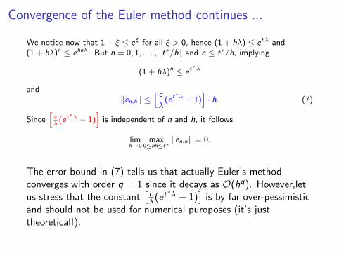
Convergence of the Euler method continues ...

We notice now that 1 + ξ ≤ eξ for all ξ > 0, hence (1 + hλ) ≤ ehλ and(1 + hλ)n ≤ ehnλ. But n = 0, 1, . . . , bt∗/hc and n ≤ t∗/h, implying

(1 + hλ)n ≤ et∗λ

and‖en,h‖ ≤

h c

λ(et∗λ − 1)

i· h. (7)

Sinceh

cλ

(et∗λ − 1)i

is independent of n and h, it follows

limh→0

max0≤nh≤t∗

‖en,h‖ = 0.

The error bound in (7) tells us that actually Euler’s methodconverges with order q = 1 since it decays as O(hq). However,letus stress that the constant

[cλ(et∗λ − 1)

]is by far over-pessimistic

and should not be used for numerical puroposes (it’s justtheoretical!).