The Pennsylvania State University

The Graduate School

Department or Electrical Engineering

MODELING AND SIMULATION OF ELECTRIC VEHICLE

ALGEBRAIC LOOP PROBLEMS REGARDING BATTERY AND FUEL CELLS

A Thesis in

Electrical Engineering

by

Zifang Mao

2014 Zifang Mao

Submitted in Partial Fulfillment

of the Requirements

for the Degree of

Master of Science

August 2014

ii

The thesis of Zifang Mao was reviewed and approved* by the following:

Jeffrey S. Mayer

Associate Professor of Electrical Engineering

Thesis Advisor

Minghui Zhu

Dorothy Quiggle Assistant Professor of Electrical Engineering

Kultegin Aydin

Professor of Electrical Engineering and Department Head

*Signatures are on file in the Graduate School

iii

ABSTRACT

Vehicles equipped with internal combustion engine (ICE) have been in existence for over

a hundred years. Although ICE vehicles (ICEVs) are being improved by modern automotive

electronics technology, they need a major change to significantly improve the fuel economy and

reduce the emissions. Electric vehicles (EVs) and hybrid EVs (HEVs) have been identified to be

the most viable solutions to fundamentally solve the problems associated with ICEVs.

This thesis is concerned with modeling and simulation of EVs. Specifically, additional

attention is paid to algebraic loops, a general problem that may occur in many other systems

besides vehicles. First, a nonlinear battery model is developed and the algebraic loop is broken by

several different methods. The simulation results are compared and analyzed. Then a PEM fuel

cell model is developed and the results from the literature are reproduced. The fuel cell model

contains a more complex algebraic problem when connected to a load other than current source.

This problem has not been talked about in the literature and some different methods are

developed and compared to deal with it. Last, an electric vehicle model is developed and previous

methods are applied to the vehicle model. The simulation results of the EV model are analyzed

and discussed as well.

Key words: Electric vehicle, battery, PEM fuel cell, linearization, algebraic loops,

MATLAB/Simulink

iv

TABLE OF CONTENTS

List of Figures .......................................................................................................................... v

List of Tables ........................................................................................................................... vii

Acknowledgements .................................................................................................................. viii

Chapter 1 Introduction ............................................................................................................. 1

Motivation ........................................................................................................................ 1 Problem Statement ........................................................................................................... 2 Organization ..................................................................................................................... 4

Chapter 2 Modeling and Simulation of Li-ion Battery ............................................................ 5

Nonlinear Battery Model with Algebraic Loop ............................................................... 8 Breaking the algebraic loop explicitly ............................................................................. 10 Adding a memory block ................................................................................................... 11 Comparison and Analysis ................................................................................................ 12 Linearization and discretization of model No.2 ............................................................... 14 Linearization of model No.3 ............................................................................................ 15 Analytical solutions to linearized system for model No.2 ............................................... 16 Analytical solution to linearized system for model No.3 ................................................. 18 Nonlinear Internal Resistance .......................................................................................... 20

Chapter 3 Fuel Cells................................................................................................................. 23

Fuel cell model ................................................................................................................. 24 Algebraic loop in fuel cell model ..................................................................................... 28

Chapter 4 Electric Vehicle ....................................................................................................... 36

Algebraic Loop in the Electric Vehicle Model Using Battery ......................................... 38 Algebraic Loop in the Electric Vehicle Model Using PEM Fuel Cells ........................... 44 Drive Cycle ...................................................................................................................... 48

Chapter 5 Conclusion ............................................................................................................... 52

Referrences....................................................................................................................... 54 Appendix A Simulink Diagrams ..................................................................................... 57 Appendix B MATLAB Scripts ....................................................................................... 60

v

LIST OF FIGURES

Figure 1-1. An example of an algebraic loop. .......................................................................... 3

Figure 2-1. Equivalent circuit of battery [16]. ......................................................................... 6

Figure 2-2. Li-ion battery model [10]. ..................................................................................... 6

Figure 2-3. Typical discharge curve [16]. ................................................................................ 7

Figure 2-4. Nonlinear battery model. ....................................................................................... 9

Figure 2-5. Response of nonlinear battery model with algebraic loop. ................................... 9

Figure 2-6. Breaking algebraic loop explicitly. ....................................................................... 11

Figure 2-7. Adding a memory block. ....................................................................................... 12

Figure 2-8. Differences between model No.2 and No.3. ......................................................... 13

Figure 2-9. Equivalent circuit. ................................................................................................. 17

Figure 2-10. Linearized model for No.3. ................................................................................. 19

Figure 3-1. The PEM fuel cell model [19]. .............................................................................. 25

Figure 3-2. Static output characteristic of PEM fuel cell. ........................................................ 26

Figure 3-3. Dynamic responses subject to step load changes: (a) a step load increase and

(b) a step load decrease. ................................................................................................... 28

Figure 3-4. PEM fuel cell with a Thevenin load. ..................................................................... 29

Figure 3-5. Calculation of initial condition. ............................................................................. 29

Figure 3-6. Voltage and Current of PEM fuel cell connected to a Thevenin load. .................. 30

Figure 3-7. Differences between systems with and without memory block. ........................... 31

Figure 3-8. Voltage and current curves of fuel cell system with linear approximation. .......... 33

Figure 3-9. Differences between linear approximation and original system. .......................... 33

Figure 3-10. Differences between quadratic approximation and the original system. ............. 34

Figure 4-1. Overall structure of electric vehicle. ..................................................................... 36

Figure 4-2. Waveforms of vehicle model using battery. .......................................................... 38

Figure 4-3. Vehicle plant with algebraic loop broken explicitly. ............................................ 40

vi

Figure 4-4. Vehicle plant with memeory block. ...................................................................... 40

Figure 4-5. Differences between model No.5 and No.6. ......................................................... 41

Figure 4-6. Waveforms of vehicle model using PEM fuel cells. ............................................. 44

Figure 4-7. Waveforms of linear approximation. .................................................................... 46

Figure 4-8. Differences between linear approximation and original system. .......................... 47

Figure 4-9. Differences between systems with and without memory block. ........................... 48

Figure 4-10. Velocity and torque. ............................................................................................ 49

Figure 4-11. Power and SOC. .................................................................................................. 49

Figure 4-12. HWFET - velocity and torque. ............................................................................ 50

Figure 4-13. HWFET – power and SOC.................................................................................. 50

Figure 4-14. NYCC – velocity and torque. .............................................................................. 51

Figure 4-15. NYCC – power and SOC. ................................................................................... 51

vii

LIST OF TABLES

Table 2-1. Battery Models Comparison ................................................................................... 12

Table 3-1. PEM fuel cell model parameters ............................................................................ 27

Table 4-1. Vehicle models comparison.................................................................................... 41

viii

ACKNOWLEDGEMENTS

First and foremost, I would like to express my sincere gratitude to my thesis supervisor,

Dr. Jeffrey Mayer in the department of Electrical Engineering, for his guidance and patience

throughout the completion of my degree. This thesis would have never materialized without his

continuous understanding and support.

In addition, I would like to thank my thesis reader, Dr. Minghui Zhu in the department of

Electrical Engineering, for his thorough review and various suggestions to improve the quality of

my thesis.

Last but not least, I would like to thank my family, my parents. No words can express my

utmost appreciation for their unconditional support, inspiration, and motivation over the years of

pursuing this degree.

Chapter 1

Introduction

Motivation

Vehicles equipped with internal combustion engine (ICE) have been in existence for over

a hundred years. Although ICE vehicles continue to be improved through modern automotive

electronics technology, they need a major change to significantly improve fuel economy and

reduce emissions. Electric vehicles (EVs) and hybrid Electric Vehicles (HEVs) have been

identified as the most viable solutions to fundamentally solve the problems associated with ICE

vehicles [1]-[4]. Hybrid electric vehicles (HEVs), battery electric vehicles (BEVs), and plug-in

hybrid electric vehicles (PHEVs) are becoming more popular. PHEVs are charged by either

plugging into electric outlets or by means of on-board electricity generation. These vehicles can

drive at full power in electric-only mode over a limited range. As such, PHEVs offer valuable

fuel flexibility [5]. PHEVs may have a larger battery and a more powerful motor compared to a

HEV, but their range is still very limited [6]-[7]. A Fuel Cell Vehicle (FCV) or Fuel Cell Electric

Vehicle (FCEV) is a type of vehicle that uses a fuel cell to power its on-board electric motor. Fuel

cells in vehicles create electricity to power an electric motor, generally using oxygen from the air

and stored hydrogen. As of 2009, motor vehicles used most of the petroleum consumed in the U.S.

and produced over 60% of the carbon monoxide emissions and about 20% of greenhouse gas

emissions in the United States. In contrast, a vehicle fueled with pure hydrogen emits few

pollutants, producing mainly water and heat, although the production of the hydrogen would

create pollutants unless the hydrogen used in the fuel cell were produced using only renewable

energy [20].

2

In order to increase the efficiency and accuracy of automotive design, Computer Aided

Engineering (CAE) has been playing an ever increasing role throughout the process of vehicle

design process. With the increase of computing power, manufacturers are now able to perform

design, testing, and optimization of a vehicle through computer simulation, all prior to the actual

manufacturing of a vehicle [8].

The purpose of this thesis is to create a MATLAB/Simulink electric vehicle model that

can be used for controller design and simulation before applying to hardware and real vehicle.

This thesis mainly focuses on the algebraic loop problem during simulation that has not been

thoroughly reported in the literature regarding vehicle modeling and simulation.

Problem Statement

An algebraic loop in a Simulink model occurs when a signal loop exists with only direct

feedthrough blocks within the loop. Direct feedthrough means that the block output depends on

the value of an input port; the value of the input directly controls the value of the output. Non-

direct-feedthrough blocks maintain a state variable. Two examples are the Integrator or Unit

Delay block.

Some Simulink blocks have input ports with direct feedthrough. The software cannot

compute the output of these blocks without knowing the values of the signals entering the blocks

at these input ports at the current time step.

An example of an algebraic loop is shown in Figure 1-1. Note that this is not a

recommended modeling pattern.

3

Figure 1-1. An example of an algebraic loop.

Mathematically, this loop implies that the output of the Sum block is an algebraic

variable xa that is constrained to equal the first input u minus xa (for example, xa = u – xa). The

solution of this simple loop is xa = u/2.

In Simulink models, algebraic loops are treated as algebraic constraints. Models with

algebraic loops define a system of differential algebraic equations (DAEs). Simulink does not

solve DAEs directly. Simulink solves the algebraic equations (the algebraic loop) numerically

for xa at each step of the ODE solver [9].

Algebraic loops may cause some problems. If the model contains an algebraic loop, we

cannot generate code for the model. The Simulink algebraic loop solver might not be able to

solve the algebraic loop. While Simulink is trying to solve the algebraic loop, the simulation

might execute slowly. Thus it worth doing some research on algebraic loops while modeling and

simulation.

This thesis begins with a Li-ion battery model which can be used as a subsystem in HEV

model and develops a series of methods to break the algebraic loop and compares the results

among them. Then the whole vehicle is modeled and simulated and the methods are applied to

this more complex HEV model. These methods can also be applied to other models containing

algebraic loops.

4

Organization

In Chapter 2, a battery model that can be used in the electrical vehicle model is developed

and analyzed. Tremblay, O. and Dessaint, L.-A., along with Dekkiche, A.-I., developed an easy-

to-use battery model in “A General Battery Model for the Dynamic Simulation of Hybrid Electric

Vehicles” in 2007. They used only the battery state-of-charge (SOC) as a state variable in order to

accurately reproduce the manufacturer’s curves for the four major types of battery chemistries

[10]. These four types are: Lead-Acid, Lithium-Ion (Li-Ion), Nickel-Cadmium (NiCd) and

Nickel-Metal-Hydride (NiMH). They described the battery model and its parameters. Later in

2009, Tremblay and Dessaint presented an improved battery dynamic model [11]. The charge and

the discharge dynamics of the battery model are validated experimentally with four batteries

types. An interesting feature of this model is the simplicity to extract the dynamic model

parameters from batteries datasheets. Only three points on the manufacturer’s discharge curve in

steady state are required to obtain the parameters. The battery model is included in the “Electrical

Sources” Library of Simulink.

In Chapter 3, A PEM fuel cell model is also studied and developed. In [19], El-Sharkh et

al. introduced an easy to use PEM fuel cell model but they assumed the temperature and internal

resistance to be constant. In [21], Zhang et al. developed the temperature and internal resistance

dynamics as functions of current, which turns out to be a more practical model. The fuel cell

model used in this thesis in based on these two papers.

In Chapter 4, an electrical vehicle model is developed using the battery and fuel cells as

subsystems. Treating the other subsystems as power load of battery or fuel cells, the focus point

of this vehicle model is still algebraic loops compared to other vehicle models in the literature.

In Chapter 5, conclusions are made and future works are illustrated.

Chapter 2

Modeling and Simulation of Li-ion Battery

A lithium-ion battery (sometimes Li-ion battery or LIB) is a member of a family

of rechargeable battery types in which lithium ions move from the negative electrode to the

positive electrode during discharge and back when charging [12]. Lithium-ion batteries are

common in consumer electronics. They are one of the most popular types of rechargeable battery

for portable electronics, with one of the best energy densities, no memory effect (note, however,

that new studies have shown signs of memory effect in lithium-ion batteries [13]), and only a

slow loss of charge when not in use. Beyond consumer electronics, LIBs are also growing in

popularity for military, electric vehicle and aerospace applications [14]. For example, Lithium-ion

batteries are becoming a common replacement for the lead acid batteries that have been used

historically for golf carts and utility vehicles. Instead of heavy lead plates and acid electrolyte, the

trend is to use a lightweight lithium/carbon negative electrodes and lithium iron phosphate

positive electrodes. Lithium-ion batteries can provide the same voltage as lead-acid batteries, so

no modification to the vehicle's drive system is required [15].

The battery block in Simulink implements a generic dynamic model parameterized to

represent most popular types of rechargeable batteries [16]. The equivalent circuit of the battery

is shown in Figure 2-1.

6

Figure 2-1. Equivalent circuit of battery [16].

The Li-ion battery is chosen to be used in the HEV system because of the advantages

mentioned above. In this case, the structure of the battery model is illustrated in Figure 2-2.

Figure 2-2. Li-ion battery model [10].

the mathematical equations are given below:

Discharge Model (i* > 0)

1 0( , *, ) * exp( ).Q Q

f q i i E K i K q A BqQ q Q q

Charge Model (i* < 0)

2 0( , *, ) * exp( ).0.1

Q Qf q i i E K i K q A Bq

q Q Q q

7

where,

EBatt = Nonlinear voltage (V)

E0 = Constant voltage (V)

Exp(s) = Exponential zone dynamics (V)

Sel(s) = Represents the battery mode. Sel(s) = 0 during battery discharge, Sel(s) = 1

during battery charging.

K = Polarization constant (Ah−1

) or Polarization resistance (Ohms)

i* = Low frequency current dynamics (A)

i = Battery current (A)

q = Extracted capacity (Ah)

Q = Maximum battery capacity (Ah)

A = Exponential voltage (V)

B = Exponential capacity (Ah)−1

[16]

A typical discharge curve is composed of three sections, as shown below:

Figure 2-3. Typical discharge curve [16].

The first section represents the exponential voltage drop when the battery is charged. The

second section represents the charge that can be extracted from the battery until the voltage drops

below the battery nominal voltage. Finally, the third section represents the total discharge of the

battery, when the voltage drops rapidly [16].

8

The model is based on specific assumptions and has limitations:

1) Model assumptions:

Internal resistance is assumed to be constant during the charge and the discharge

cycles and doesn't vary with the amplitude of the current.

Model parameters are deduced from discharge characteristics and assumed to be

the same for charging.

Battery capacity doesn't change with the amplitude of current (No Peukert effect).

Temperature dependence is not included.

Self-Discharge is not represented. It can be represented by adding a large

resistance in parallel with the battery terminals.

The battery has no memory effect.

2) Model limitations:

The minimum no-load battery voltage is 0 volt and the maximum battery voltage

is equal to 2E0.

The minimum capacity of the battery is 0 Ah and the maximum capacity is Qmax.

Nonlinear Battery Model with Algebraic Loop

The proposed model represents a nonlinear voltage which depends uniquely on the actual

battery charge. If one applies this battery model to an external voltage source and a resister, a

warning regarding algebraic loops appears when simulating. This is caused by the internal

resistance. On this signal path, all the blocks are direct feedthrough blocks, as shown in Figure 2-

4.

9

The nominal voltage of this battery is 3.3V. The initial state of charge is 80%. The

external voltage source is a step input from 3.25 V to 3.2 V at t = 20000 s. The battery

discharges from the initial time t = 0 until its voltage reaches the external voltage, 3.25 V.

This is the 1st steady state. Then at t = 20000 s, as the external voltage drops, the 2

nd

transient begins. Finally the system reaches the 2nd

steady state until the battery voltage is

equal to 3.2 V.

Figure 2-4. Nonlinear battery model.

The voltage, state of charge, and current waveforms are shown in Figure 2-5.

Figure 2-5. Response of nonlinear battery model with algebraic loop.

0 1 2 3

x 104

3.18

3.2

3.22

3.24

3.26

3.28

3.3

3.32

3.34

Voltage

t

V

0 1 2 3

x 104

0

10

20

30

40

50

60

70

80State of Charge

t

%

0 1 2 3

x 104

0

0.1

0.2

0.3

0.4

0.5

0.6

0.7

0.8

0.9

1Current

t

A

10

Although MATLAB/Simulink can solve this algebraic loop, it takes longer time to get the

results. The average simulation time of this model is 1.73 s.

Breaking the algebraic loop explicitly

The algebraic loop is caused only by the internal resistance. Every signal path inside the

nonlinear subsystem contains at least one non-direct feedthrough block (e.g., integral or low pass

filter). To break the algebraic loop explicitly, we need to develop a new set of equations to

describe the same system and then reformat the blocks accordingly.

The original system is described by

2

(1)

( ) (2)

batt batt batt

batt

V E iR

i g V V

Substituting (2) into (1),

2

2

2

2

( )

(1 )

1

batt batt batt batt

batt batt batt batt

batt batt batt batt

batt battbatt

batt

V E g V V R

E gR V gR V

gR V E gR V

E gR VV

gR

and

22 2( )

1

batt battbatt

batt

E gR Vi g V V g V

gR

.

Therefore the system can be reformatted as shown in Figure 2-6.

11

Figure 2-6. Breaking algebraic loop explicitly.

In this model, all the signal paths go through the nonlinear subsystem, which contains no

direct feedthrough loops. Therefore the algebraic loop is broken explicitly. The results from this

model are accurate and the simulation time is the least.

Adding a memory block

The simplest method to avoid the algebraic loop warning is to add a non-direct

feedthrough block on the signal path, for example, a memory block, as shown in Figure 2-7.

But adding an additional block only to avoid algebraic loop is not recommended when

modeling. The memory block may change the system dynamics and introduce additional time

delay. Thus causes the results less accurate and longer simulation time.

12

Figure 2-7. Adding a memory block.

Comparison and Analysis

We have discussed three battery models with Thevenin load so far. To compare the

simulation time, each model has been runned multiple times and the mean values of execution

time are computed and recorded in Table 2-1.

Table 2-1. Battery Models Comparison

Model No. Model description Average simulation time

1 Battery with Thevenin load

Algebraic loop 1.73 s

2 Battery with Thevenin load

Breaking algebraic loop explicitly 0.88 s

3 Battery with Thevenin load

Adding memory block 1.11 s

It is the fastest to analyze the system and reformat it to a form without algebraic loops.

Adding a memory block do slower the simulation process by 27%. But still it’s better than

leaving the algebraic loop for MATLAB/Simulink to solve.

13

Adding a memory block also introduces extra error to the system. The differences

between model No.2 and No.3 are plotted in Figure 2-8. These data are generated under the

condition of simulation step size = 1. The voltage and current errors mainly occur at the

beginning of each transient. The state of charge error lasts longer but reaches zero when the

system enter stead state. The memory block changes the system dynamics thus introduces extra

error in transient. The error is caused mainly by the unit time delay. From the engineering point

of view, since the model is always an approximation of real world, the error caused by memory

block is tolerable. But it is still worth researching how does the memory block change the internal

dynamics of the system, so that we have a thorough understanding of adding this block.

Figure 2-8. Differences between model No.2 and No.3.

To analyze more thoroughly, we linearize model No.2 and No.3. The operating point is

chosen to be the 1st steady state, which means Vbatt = 3.25V and i = 0.

0 1 2 3

x 104

-2

0

2

4

6

8

10

12x 10

-3 Voltage

t

V

0 1 2 3

x 104

-2

0

2

4

6

8

10

12

14x 10

-3 State of Charge

t

%

0 1 2 3

x 104

-0.02

0

0.02

0.04

0.06

0.08

0.1

0.12Current

t

A

14

Linearization and discretization of model No.2

The linearized state space description of model No.2 is given by Simulink using the linear

analysis toolbox.

2 2

2 2

x = A x + B u

y = C x + D u

where

2

*, ,

battVi

V SOCq

i

x u y

and

2 2

2 2

0.1528 0.001119 9.091,

0.05275 0.001119 9.091

0.005275 0.0001119 0.09091

0 0.01208 , 0 .

0.05275 0.001119 9.091

A B

C D

This is a continuous-time model. The eigenvalues of A2 are c1 = -0.1531 and c2 = -0.0007.

Converting it to discrete-time model using sample time T = 1, which is the same as the

simulation step size, we get

2 2

2 2

[ 1] [ ] [ ]

[ ] [ ] [ ]

d d

d d

k k k

k k k

x A x B u

y C x D u

where

2 2

2 2

0.8584 0.001037 8.426,

0.0489 0.9989 8.858

0.005275 0.0001119 0.09091

0 0.01208 , 0

0.05275 0.001119 9.091

d d

d d

A B

C D

15

The eigenvalues of A2d are d1 = 0.8580 and d2 = 0.9993.

The relationships between the eigenvalues of these two linear systems are 1

1c T

d e and

2

2c T

d e .

Linearization of model No.3

On the other hand, the linearized state space description of model No.3 is given by

Simulink using linear analysis toolbox.

3 3

3 3

[ 1] [ ] [ ]

[ ] [ ] [ ]

k k k

k k k

x A x B u

y C x D u

where

2

*, ,

battVi

V SOCq

i

x u y

and

3 3

3 3

0.8546 0.001065 8.651,

0.05275 0.9989 9.091

0.005275 0.0001119 0.09091

0 0.01208 , 0 .

0.05275 0.001119 9.091

A B

C D

This is a discrete-time model. The eigenvalues of A3 are 3 = -0.8542 and 4 = -0.9993.

Note that 3 and d1 are not identical, although quite close. This indicates that adding a

memory block not only discretizes the original continuous-time system, but also introduces extra

error.

16

Analytical solutions to linearized system for model No.2

The equations describing the linearized open circuit battery model are

1 1

2

2

(3)

(4)

100 (5)

( ) (6)

batt

batt

x i

V c x d i k

SOC c x

i g V V

where x is the state variable and V2 is the external voltage.

Note that the algebraic loop lies in equations (4) and (6) because both Vbatt and i are

functions of each other.

Substituting (6) into (3), we derive

2

1 1 2

1 1 2

1 1 2

1 2

1

( )

( )

( )

(1 ) ( )

( ) (7)1

battx g V V

x g c x d i k V

x g c x d x k V

gd x g c x k V

gx c x k V

gd

and

1 1

2 100

battV c x d x k

SOC c x

i x

Alternatively, we can derive these equations from circuit analysis rather than

algebraically. From (4), we can define Voc = c1x+k, thus Vbatt = Voc +d1i. Compared to the original

model, Voc actually stands for Ebatt and d1 stands for the negative of internal resistance. Then we

get the equivalent circuit shown in Figure 2-9.

17

Figure 2-9. Equivalent circuit.

Therefore,

2

1

1 2

1

1( )

1/

( )1

oci V Vd g

gx c x k V

gd

which is the same as equation (7).

To realize the standard state space form, we can take the constant terms as system

inputs. From (7), we have,

12

1 1 11 1 1

gc g gx x k V

gd gd gd

1 1

11 1 2

1 1 1

1 1 1 11 2

1 1 1

1 12

1 1 1

( )1 1 1

( ) ( 1)1 1 1

1

1 1 1

battV c x d x k

gc g gc x d x k V k

gd gd gd

gd c gd gdc x k V

gd gd gd

c gdx k V

gd gd gd

2 100SOC c x

i x

or write in the matrix form

18

x = Ax + Bu

y = Cx + Du

where

2 ,

100

battk V

V SOC

i

u y

and

1

1 1 1

1 1

1 1 1

2

1

1 11

, 01 1 1

10

1 1 1

, 0 0 1 .

01 11

gc g g

gd gd gd

c gd

gd gd gd

c

gc g g

gd gdgd

A B

C D

Given initial condition x(0) and input u(t), we can solve the system by

( )

0

( )

0

( ) (0) ( )

( ) (0) ( ) ( )

tt t

tt t

t e e d

t e e d t

A A

A A

x x Bu

y C x C Bu Du

Analytical solution to linearized system for model No.3

The linearized system for model No.3 is illustrated in Figure 2-10.

19

Figure 2-10. Linearized model for No.3.

Based on the input-output relation of memory block, the state equation describing this

system for time instances between consecutive sample points is

1 1 2( ) ( ) ( ) , ( 1) , 0, 1, 2, x t g c x t d i nT k V nT t n T n

Given initial conditions x(nT) and i(nT), the solution is given by

1 1( ) ( ) 1 2

1

( )( ) ( ) 1 , ( 1) , 0, 1, 2,

gc t nT gc t nT d i nT k Vx t e x nT e nT t n T n

c

Therefore, the equations describing the system at sample points are

1 1

1

1 1

1

1 1 1

12

1 1

1 1 2

11 2 1 2

1 1

1 1 2

( 1) 1[ 1] [ ] [ ] ( )

[ 1] [ 1] [ ] [ ]

( 1) 1[ ] [ ] ( ) [ ] ( )

[ ] [ ] ( )

gc T gc Tgc T

gc T gc Tgc T

gc T gc T gc T

e d ex n e x n i n k V

c c

i n gc x n gd i n g k V

e d egc e x n i n k V gd i n g k V

c c

gc e x n gd e i n ge k V

or in matrix form

2

( 1) ( )

( 1) ( )d d

kx n x n

Vi n i n

A B

20

where

1 1 1

1

1 1 1 1

1

1 1 1

1 1

( 1) 1 1

,

gc T gc T gc Tgc T

d d

gc T gc T gc T gc T

e d e ee

c c c

gc e gd e ge ge

A B .

This is a discrete time state space description. The solution to this system is given by

11

0 2

( ) (0)

( ) (0)

nn n j

d d

j

kx n x

Vi n i

A A B

and

1 1

2 100

battV c x d i k

SOC c x

.

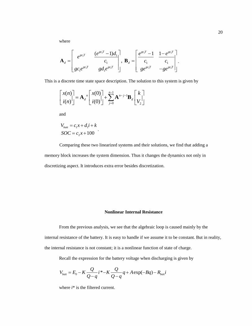
Comparing these two linearized systems and their solutions, we find that adding a

memory block increases the system dimension. Thus it changes the dynamics not only in

discretizing aspect. It introduces extra error besides discretization.

Nonlinear Internal Resistance

From the previous analysis, we see that the algebraic loop is caused mainly by the

internal resistance of the battery. It is easy to handle if we assume it to be constant. But in reality,

the internal resistance is not constant; it is a nonlinear function of state of charge.

Recall the expression for the battery voltage when discharging is given by

0 * exp( )batt batt

Q QV E K i K q A Bq R i

Q q Q q

where i* is the filtered current.

21

The coefficient before i* stands for a nonlinear polarization resistance which is a function of

battery state of charge. The use of the current filter solves the algebraic loop problem caused by

this term [11].

In other commonly used battery models, there are no current filters, thus the algebraic

loop contains nonlinear terms caused by nonlinear internal resistance. For instance, in [17] and

[18] the internal resistance is expressed in a polynomial of charge or state of charge, i.e.,

2 3 4 5

0 1 2 3 4 5( )battR f q a a q a q a q a q a q . Thus ( )batt ocV V f q i . If the battery is

connected to a Thevenin load, i.e., an external voltage source in series with a conductor,

2

2

2

2

( )

( ) ( )

(1 ( )) ( )

( )

1 ( )

batt

batt oc batt

batt oc

ocbatt

i g V V

V V f q g V V

gf q V V gf q V

V gf q VV

gf q

2

22

2

( )

( )

1 ( )

( )

1 ( )

batt

oc

oc

i g V V

V gf q Vg V

gf q

g V V

gf q

If the battery is connected to a power load,

2

2

2

( )

( )

( ) 0

4 ( )

2 ( )

batt oc

oc

oc

oc oc

P Pi

V V if q

iV i f q P

f q i V i P

V V f q Pi

f q

22

Since the current should increase if the power load increases, the negative sign should be

taken. Thus

2 4 ( )

2 ( )

oc ocV V f q Pi

f q

and

2 4 ( )

2

oc oc

batt

V V f q PV

.

Therefore, for the battery model without current filter and its internal resistance expressed

as a function of charge, the algebraic loop can also be solved explicitly, albeit approximately.

If the internal resistance is a function of current, then it may be difficult to solve the

algebraic loop explicitly. In this case, the use of filtered current provides a method to simplify this

problem while maintaining the battery characteristics.

23

Chapter 3

Fuel Cells

The ever increasing demand for electrical energy and the intense competition between

electric companies in the new electric utility market has intensified research in alternative sources

of electrical energy that are reliable and cost effective. The fuel cell, as a renewable energy source,

is considered one of the most promising sources of electric power. Fuel cells are not only

characterized by higher efficiency than conventional power plants, but they are also

environmentally clean, have extremely low emission of oxides of nitrogen and sulfur and have

very low noise [19].

Fuel cells are made up of three parts: an electrolyte, an anode and a cathode. In principle,

a hydrogen fuel cell functions like a battery, producing electricity, which can run an electric

motor. Instead of requiring recharging, however, the fuel cell can be refilled with hydrogen.

Different types of fuel cells include polymer electrolyte membrane fuel cells, direct methanol fuel

cells, phosphoric acid fuel cells, molten carbonate fuel cells, solid oxide fuel cells, and

regenerative fuel cells.

There are fuel cell vehicles for all modes of transport. The most prevalent fuel cell

vehicles are forklifts and material handling vehicles. Although there are currently no fuel cell cars

available for commercial sale, over 20 FCEVs prototypes and demonstration cars have been

released since 2009. Automobiles such as the GM HydroGen4, Honda FCX Clarity, Toyota

FCHV-adv and Mercedes-Benz F-Cell are all pre-commercial examples of fuel cell electric

vehicles. Fuel cell electric vehicles have driven more than 3 million miles, with more than 27,000

refuelings [20].

24

There are many papers discussing the models for proton exchange membrane (PEM) fuel

cells. PEM fuel cells generally operate at lower pressure and lower temperature with higher

power density compared to other types of fuel cells. Therefore, they are more suitable for

applications in small to medium power levels, such as fuel cell powered automobiles or micro-

grid power applications [21].

In this chapter, a PEM fuel cell model based on [19] and [21] is developed and the static

and dynamic characteristics are reproduced using the parameters and load conditions those two

papers provided. Then further studies of initialization and algebraic loop problem are analyzed

and results are compared.

Fuel cell model

In [19], El-Sharkh et al. introduced a model that describes the polarization curves for the

PEM fuel cell where the fuel cell voltage is the sum of three terms, the Nernst instantaneous

voltage E in terms of gas molarities, activation over voltage act, and ohmic over voltage ohmic. In

mathematical form, polarization curves can be expressed by the equation:

cell act ohmicV E (8)

Where act is a function of the oxygen concentration CO2 and stack current I (A), and ohmic is a

function of the stack current and the stack internal resistance Rint (). Assuming constant

temperature and oxygen concentration, (8) can be rewritten as (9):

intln( )cellV E B CI R I (9)

The Nernst voltage in terms of gas molarities can be written as:

25

2 2

2

0.5

0 0 ln2

H O

H O

p pRTE N E

F p

(10)

where E0 is the open cell voltage (V) and R is the universal gas constant (J (kmol K)−1).

The fuel cell model can be drawn as in Figure 3-1.

Figure 3-1. The PEM fuel cell model [19].

To design an adequate fuel cell based distributed power generation system to

accommodate different load changes, it is essential to have an accurate dynamic model for the

fuel cell system so that adequate control systems can be designed to meet the load demand. In

such a situation, the dynamics of the internal resistance characteristics of fuel cells have to be

considered. El-Sharkh et al. assumed the internal resistance to be constant. In fact, the internal

resistance will have effects on the static and dynamic characteristics of the fuel cell output. In

[21], Zhang et al. described the characteristics of the equivalent internal resistance as a nonlinear

function of stack current:

int 0 exp ln( )fc

R R fc

R

IR A R B I

(11)

26

where Rint is the equivalent internal resistance; AR, BR, R0 andτ R are all empirical parameters.

To achieve reasonably accurate representation, the following values have been selected: AR = 0.82,

BR = 0.13, R0 = 0.8, andτ R = 5 [21].

The amount of hydrogen flow required to meet the load change is given by

2

0

2H

N Iq

FU , where U is utilization rate.

The oxygen flow is considered using the hydrogen, oxygen flow ratio, rh-o.

Based on equations (9), (10) and (11) , a dynamic model of PEM fuel cell, that includes

the effects of internal resistance variations has been developed.

The static output characteristic (Voltage-Current relation) is shown in Figure 3-2. Model

parameters extracted from Fig. 9 in [21] by curve fitting and are referred to Table 1 in [19] and

are listed in Table 3-1.

Figure 3-2. Static output characteristic of PEM fuel cell.

0 10 20 30 40 50 6024

26

28

30

32

34

36

38

40

42

Current(A)

Vo

lta

ge

(V)

27

Table 3-1. PEM fuel cell model parameters

Stack Temperature, (K) 343

Faraday’s constant, F (C(kmol)-1

) 96485339

Universal gas constant, R (J(kmol)-1

K) 8314.47

No load voltage, E0 (V) 0.6

Number of cells, N0 78

Kr constant = N0/4F (kmol s-1

A) 2.02×10-7

Utilization factor, U 0.8

Hydrogen valve constant, kH2 (kmol s-1

atm) 4.22×10-5

Water valve constant, kH2O (kmol s-1

atm) 7.716×10-6

Oxygen valve constant, kO2 (kmol s-1

atm) 2.11×10-5

Hydrogen time constant τ H2 (s) 3.37

Water time constant τ H2O (s) 18.418

Oxygen time constant τ O2 (s) 6.74

Activation voltage constant, B (A-1

) 0.35

Activation voltage constant, C (V) 0.0136

Hydrogen-Oxygen flow ratio, rh-o 1.168

To validate the dynamic characteristics of the output voltage with respect to load changed,

a step load increase from 0.1 A to 30 A and a step load decrease from 30 A to 0.1 A has been

carried out. The results are shown in Figure 3-3. They are good matches to the results from [21].

In this case, the load is a current source. Thus there is no algebraic loop problem. In

reality, when the fuel cell is connected to a Thevenin load or power load, this problem appears.

28

(a) (b)

Figure 3-3. Dynamic responses subject to step load changes: (a) a step load increase and

(b) a step load decrease.

Algebraic loop in fuel cell model

Since the fuel cell voltage is a function of current, there exists the algebraic loop problem

when the fuel cell is connected to a load other than current source. For instance, when the fuel

cell is connected to a Thevenin load, the system is described by:

int

2

ln( )

( ).

cell

cell

V E B Ci R i

i g V V

V2 is an external voltage source steps from 0 to 15 V at t = 0. The simulation system is

shown in Figure 3-4.

0 20 40 60 80 10028

30

32

34

36

38

40

42Voltage

Time(s)

V

0 20 40 60 80 10030

32

34

36

38

40

42

44

46Voltage

Time(s)

V

29

Figure 3-4. PEM fuel cell with a Thevenin load.

The transfer function blocks are changed to state space description in order to specify

appropriate positive initial conditions. These initial conditions can be calculated by replacing the

state space descriptions (or first order transfer function blocks originally) with gain blocks. Then

plot the voltage-current relations of the fuel cell and the load on the same figure. The point of

intersection stands for the initial current and voltage at steady state. In our case, V2 is 0 before t =

0 and the resistance is 10 . Thus the V-I relation for the Thevenin load is V = 10I (12),

which is a straight line as shown in Figure 3-5.

Figure 3-5. Calculation of initial condition.

0 10 20 30 40 50 6024

26

28

30

32

34

36

38

40

42

44

Current(A)

Voltage(V

)

30

The point of intersection can be calculated by combining equations (9), (10), (11) and

(12).Using the “fzero” function, MATLAB returns the result that the current equals 3.85 A and

the voltage equals 38.54 V in Figure 3-5. Once we have the current and the voltage, we can use

equations (9), (10) and (11) to calculate the initial conditions for the state space description

blocks.

We simulate the dynamic system with Thevenin load from t = -10 s to t = 50 s. The

voltage and current curves are shown in Figure 3-6. As expected, the voltage and current hold at

the initial values we calculated before the external voltage V2 steps to 15 V at t = 0. This

simulation gives an algebraic loop warning.

Figure 3-6. Voltage and Current of PEM fuel cell connected to a Thevenin load.

We can avoid the algebraic loop problem by adding a memory block on the signal path of

current. The differences between the systems with and without memory block are plotted in

Figure 3-7. The main error occurs at the time when the sudden external voltage change applies.

-10 0 10 20 30 40 5038.4

38.6

38.8

39

39.2

39.4

39.6

39.8Voltage

Time(s)

V

-10 0 10 20 30 40 502.4

2.6

2.8

3

3.2

3.4

3.6

3.8

4Current

Time(s)

A

31

Figure 3-7. Differences between systems with and without memory block.

To solve the algebraic loop explicitly without adding a memory block, we have

int 2( ln( ) )i g E B Ci R i V

int 2ln( ) ( )gB Ci i gR i g E V

Using the expression for Rint in (11), we have

0 2ln( ) ln( ) ( )R

i

R RgB Ci i gi A R e B i g E V

0 2(1 ) ln( ) ln( ) ( )R

i

R RgA i gR ie gB i i gB Ci g E V

(13)

This is a transcendental equation with respect to current. There is no explicit solution to this

equation. We can use Taylor series as an approximation in the neighborhood of some operating

point to get analytical solution near that point.

Let f(i) be the left hand side of equation (13). The Taylor series near operating point i0 are

-10 0 10 20 30 40 50-1.2

-1

-0.8

-0.6

-0.4

-0.2

0

0.2Voltage

Time(s)

V

-10 0 10 20 30 40 50-0.2

0

0.2

0.4

0.6

0.8

1

1.2

1.4Current

Time(s)

A

32

0

0 0

0 0

200 0 0 0

0 0 0 0 0 0

00 0 0

0

00 2

0

''( )( ) ( ) '( )( ) ( )

2!

(1 ) ln( ) ln( )

(1 ) ln( ) 1 ( )

1

2 2 2

R

R R

R R

i

R R

i i

R R

R

i i

R

R R

f if i f i f i i i i i

gA i gR i e gB i i gB Ci

i gBgA gR e e gB i i i

i

i B Bg R e e

i i

0

2

02

0

1 00 01 1

0 0

( )

1 ( 1) ( )

( 1)! ! ( 1)R

i

n nR

n n n n

R R

i i

i B Bg R e i i

n n n n i ni

If we use a linear approximation, i.e., 0 0 0 2( ) ( ) '( )( ) ( )f i f i f i i i g E V , then the explicit

solution to this linear equation is given by

0

0 0

2 00

0

2 0 0 0 0 0 00

00 0

0

( ) ( )

'( )

( ) [(1 ) ln( ) ln( )] (14)

(1 ) ln( ) 1

R

R R

i

R R

i i

R R

R

g E V f ii i

f i

g E V gA i gR i e gB i i gB Cii

i gBgA gR e e gB i

i

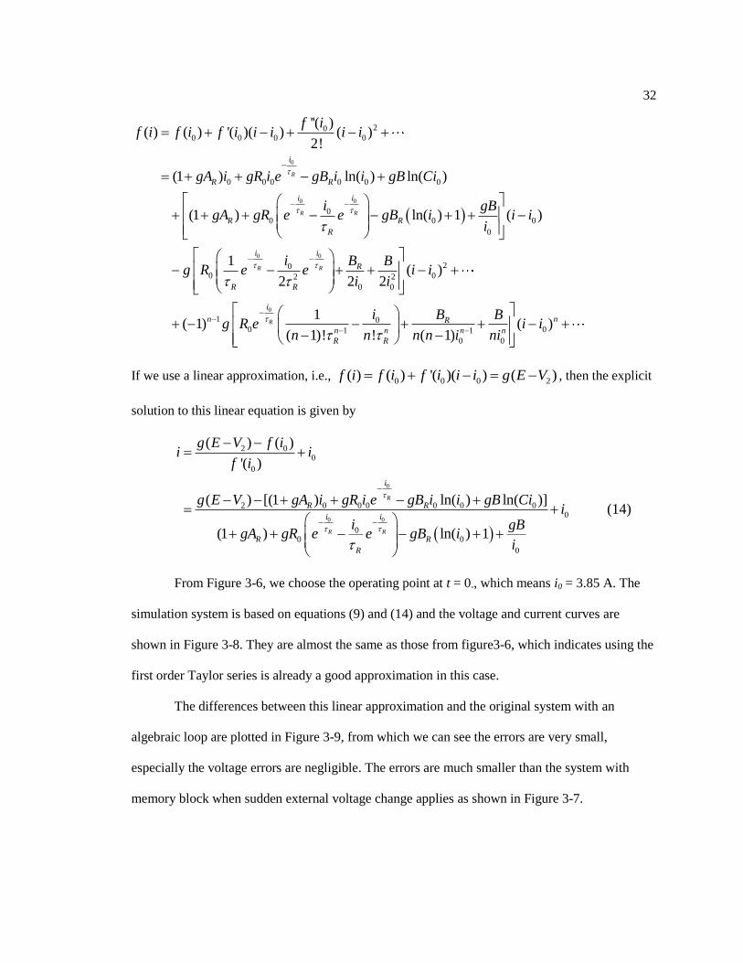
From Figure 3-6, we choose the operating point at t = 0-, which means i0 = 3.85 A. The

simulation system is based on equations (9) and (14) and the voltage and current curves are

shown in Figure 3-8. They are almost the same as those from figure3-6, which indicates using the

first order Taylor series is already a good approximation in this case.

The differences between this linear approximation and the original system with an

algebraic loop are plotted in Figure 3-9, from which we can see the errors are very small,

especially the voltage errors are negligible. The errors are much smaller than the system with

memory block when sudden external voltage change applies as shown in Figure 3-7.

33

Figure 3-8. Voltage and current curves of fuel cell system with linear approximation.

Figure 3-9. Differences between linear approximation and original system.

If we use a second order approximation, i.e.,

200 0 0 0 2

''( )( ) ( ) '( )( ) ( ) ( )

2

f if i f i f i i i i i g E V ,

then we can solve this quadratic equation explicitly.

-10 0 10 20 30 40 5038.4

38.6

38.8

39

39.2

39.4

39.6

39.8Voltage

Time(s)

V

-10 0 10 20 30 40 502.4

2.6

2.8

3

3.2

3.4

3.6

3.8

4Current

Time(s)

A

-10 0 10 20 30 40 50-2

0

2

4

6

8

10

12

14

16x 10

-3 Voltage

Time(s)

V

-10 0 10 20 30 40 50-0.018

-0.016

-0.014

-0.012

-0.01

-0.008

-0.006

-0.004

-0.002

0Current

Time(s)

A

34

200 0 0 0 2

''( )( ) '( )( ) ( ) ( ) 0

2

f ii i f i i i f i g E V

2

0 0 0 0 2

0

0

'( ) '( ) 2 ''( )[ ( ) ( )]

''( )

f i f i f i f i g E Vi i

f i

(15),

Where

0

0 0 0 0 0 0 0( ) (1 ) ln( ) ln( )R

i

R Rf i gA i gR i e gB i i gB Ci

0

00 0 0

0

'( ) (1 ) 1 ln( ) 1R

i

R R

R

i gBf i gA gR e gB i

i

0

00 0 2 2

0 0

1''( )

2 2 2R

i

R

R R

i B Bf i g R e

i i

.

The differences between this quadratic approximation and the original system are shown

in Figure 3-10. They are smaller than those illustrated in Figure 3-9.

Figure 3-10. Differences between quadratic approximation and the original system.

The quadratic approximation can reduce the error by 40% compared to the linear

approximation. But note that the maximum error is already less than 0.4% of the variable

-10 0 10 20 30 40 50-2

0

2

4

6

8

10x 10

-3 Voltage

Time(s)

V

-10 0 10 20 30 40 50-0.01

-0.009

-0.008

-0.007

-0.006

-0.005

-0.004

-0.003

-0.002

-0.001

0Current

Time(s)

A

35

magnitude; we can say that there is no need to add more higher order terms in the Taylor series

approximation.

In summary, the proposed fuel cell system stands for a system that contains an algebraic

loop problem more complex than the battery system. To break the nonlinear algebraic loop (i.e.,

including transcendental equations), one can either add a non-direct feedthrough block (i.e.,

memory block) or solve it explicitly by using Taylor series approximation around some operating

point. When the neighborhoods of some specific points are of more concern than the entire

solution space, breaking the algebraic loop explicitly by some approximation may be a better

choice. In the proposed model with a Thevenin load, even a linear approximation is more

accurate than adding a memory block, especially when some sudden load change occurs.

Chapter 4

Electric Vehicle

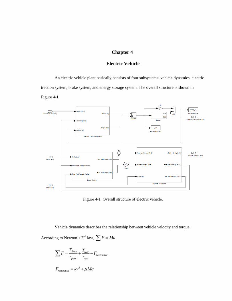
An electric vehicle plant basically consists of four subsystems: vehicle dynamics, electric

traction system, brake system, and energy storage system. The overall structure is shown in

Figure 4-1.

Figure 4-1. Overall structure of electric vehicle.

Vehicle dynamics describes the relationship between vehicle velocity and torque.

According to Newton’s 2nd

law, F Ma .

tan

front rearresis ce

front rear

T TF F

r r

2

tanresis ceF kv Mg

37

v adt

The electric traction system computes the product of required torque and wheel rotation

velocity and compares to the maximum power it could provide. If the required power is less than

the maximum power, the electric traction system outputs the required torque and power.

Otherwise the output torque has to be less than required.

required requiredP T

0

, if <

/ , if

required required 0

out

required 0

T P PT

P P P

outout

TP

where stands for the efficiency.

The brake system identifies the polarity of velocity and outputs extra resistant torque to

slow the vehicle down. If in full brake, the vehicle can stop within 180 feet from the initial

velocity of 60 mph.

The energy storage system can be a battery or PEM fuel cell. The battery’s rated voltage

is 300 V and the rated capacity is 60 Ah.

In this vehicle model, the other three subsystems can be treated as the power load of the

battery or fuel cell.

Algebraic Loop in the Electric Vehicle Model Using Battery

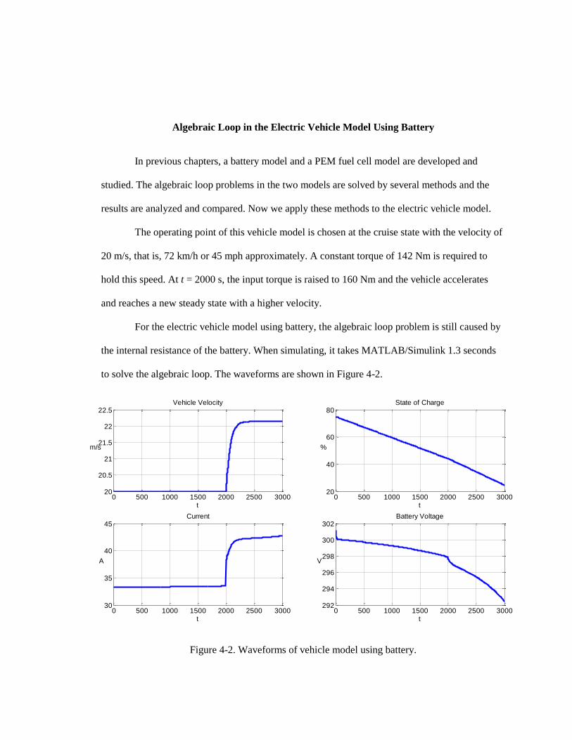
In previous chapters, a battery model and a PEM fuel cell model are developed and

studied. The algebraic loop problems in the two models are solved by several methods and the

results are analyzed and compared. Now we apply these methods to the electric vehicle model.

The operating point of this vehicle model is chosen at the cruise state with the velocity of

20 m/s, that is, 72 km/h or 45 mph approximately. A constant torque of 142 Nm is required to

hold this speed. At t = 2000 s, the input torque is raised to 160 Nm and the vehicle accelerates

and reaches a new steady state with a higher velocity.

For the electric vehicle model using battery, the algebraic loop problem is still caused by

the internal resistance of the battery. When simulating, it takes MATLAB/Simulink 1.3 seconds

to solve the algebraic loop. The waveforms are shown in Figure 4-2.

Figure 4-2. Waveforms of vehicle model using battery.

0 500 1000 1500 2000 2500 300020

20.5

21

21.5

22

22.5Vehicle Velocity

t

m/s

0 500 1000 1500 2000 2500 300020

40

60

80State of Charge

t

%

0 500 1000 1500 2000 2500 300030

35

40

45Current

t

A

0 500 1000 1500 2000 2500 3000292

294

296

298

300

302Battery Voltage

t

V

39

We can see that as the input torque steps up, so do the vehicle velocity and current. They

reach new steady state after approximately 4 minutes. The battery voltage and state of charge

keeps going down, but at different rates.

The equations describing the battery part are

(16)

(17)

batt batt batt

batt

V E iR

Pi

V

Substituting (16) into (17),

batt batt

Pi

E iR

. Therefore,

2

2 0

batt batt

batt batt

iE i R P

R i E i P

2 4

2

batt batt batt

batt

E E R Pi

R

Since the current should increase if the required power increases, the negative sign should

be picked. Thus

2 4

2

batt batt batt

batt

E E R Pi

R

and

2 4 (18)

2

batt batt batt

batt

E E R PV

.

Using this expression (18) instead of (16) to reformat the vehicle model, we can eliminate

the algebraic loop, as shown in Figure 4-3.

40

Figure 4-3. Vehicle plant with algebraic loop broken explicitly.

Besides the analytical method, a memory block can be added on the current path of the

original vehicle model to avoid the algebraic loop warning, as shown in Figure 4-4. But again this

is not recommended because it changes the dynamics and slows the simulation process.

Figure 4-4. Vehicle plant with memeory block.

41

To compare the simulation time, each vehicle model has been runned multiple times and

the mean values of execution time are computed and recorded in Table 4-1.

Table 4-1. Vehicle models comparison

Model No. Model description Average simulation time

4 Vehicle model with algebraic loop 1.36 s

5 Reformatted vehicle model

Breaking algebraic loop explicitly 0.24 s

6 Vehicle model

Adding memory block 0.32 s

Compared to model No.5, adding a memory block slows the simulation process by 35%.

To compare the errors the memory block introduced, we plot the differences of the

waveforms from model No.5 and No.6 in Figure 4-4. The errors are minor; mainly occur when

the sudden load change applies because of the unit delay characteristic of the memory block.

Figure 4-5. Differences between model No.5 and No.6.

0 500 1000 1500 2000 2500 3000-0.5

0

0.5Vehicle Velocity

t

m/s

0 500 1000 1500 2000 2500 30000

0.005

0.01

0.015

0.02

0.025State of Charge

t

%

0 500 1000 1500 2000 2500 3000-0.05

-0.04

-0.03

-0.02

-0.01

0Current

t

A

0 500 1000 1500 2000 2500 30000

0.1

0.2

0.3

0.4Battery Voltage

t

V

42

To analyze more thoroughly, we linearize model No.5 and No.6 respectively at the cruise

speed of 20 m/s. The linearized state space description of model No.5 is given by Simulink using

linear analysis toolbox.

5 5

5 5

x = A x + B u

y = C x + D u

Where

*

, , required

batt

vi

SOCq T

iv

V

x u y

and

6

4 6

5 5

0.0997 1.462 10 1.67 0.2359

3.049 10 1.462 10 1.67 , 0.2359

0 0 0.01333 0.001634

A B

4

5 54 6

5

0 0 1 0

0 4.63 10 0 0,

3.049 10 1.462 10 1.67 0.2359

0.002757 1.322 10 0.06679 0.009435

C D .

This is a continuous-time model. The eigenvalues of A5 are c1 = -0.0997, c2 = -0.0133,

and c3 = 0. Converting it to discrete-time model using sample time T = 1, which is the same as

the simulation step size, we get

5 5

5 5

[ 1] [ ] [ ]

[ ] [ ] [ ]

d d

d d

k k k

k k k

x A x B u

y C x D u

where

43

6

4

5 5

4

5 54 6

5

0.9051 1.392 10 1.578 0.2258

2.902 10 1 1.659 , 0.2373

0 0 0.9868 0.001623

0 0 1 0

0 4.63 10 0 0,

3.049 10 1.462 10 1.67 0.2359

0.002757 1.322 10 0.06679 0.009435

d d

d d

A B

C D

The eigenvalues of A5d are d1 = 0.9051, d2 = 0.9868, and d3 = 1.

Note that 1

1c T

d e , 2

2c T

d e , and 3

3c T

d e .

On the other hand, the linearized state space description of model No.6 is given by

6 6

6 6

[ 1] [ ] [ ]

[ ] [ ] [ ]

k k k

k k k

x A x B u

y C x D u

where

*

, , required

batt

vi

SOCq T

iv

V

x u y

and

7

4

6 6

4

6 64 7

6

0.9023 9.318 10 1.573 0.2229

3.006 10 1 1.658 , 0.2342

0 0 0.9868 0.001623

0 0 1 0

0 4.63 10 0 0,

3.006 10 9.791 10 1.658 0.2342

0.002756 8.98 10 0.06631 0.009367

A B

C D .

This is a discrete-time model. The eigenvalues of A6 are 1 = 0.9023, 2 = 0.9868 and 3 = 1.

44

We can see that 1 is not equal to d1.This indicates that the memory block not only

discretize the original continuous-time system, but also alters the internal dynamics.

Algebraic Loop in the Electric Vehicle Model Using PEM Fuel Cells

To replace the battery by PEM fuel cells in the electric vehicle system, we increase the

number of cells to ensure the capability of power meet the demand of the vehicle load.

The operating conditions are the same as the one using battery. First, the input torque is

set to 141 Nm to hold the velocity of 20 m/s. Then the input torque is raised to 160 Nm and the

vehicle accelerates and reaches a new steady state with a higher velocity.

The waveforms of vehicle velocity, fuel cell current and voltage are shown in Figure 4-6.

Figure 4-6. Waveforms of vehicle model using PEM fuel cells.

0 200 40020

20.5

21

21.5

22

22.5Vehicle Velocity

t

m/s

0 200 40046

48

50

52

54

56

58

60

62Current

t

A

0 200 400208

208.2

208.4

208.6

208.8

209

209.2

209.4

209.6

209.8

210Fuel Cell Voltage

t

V

45

The equations describing the algebraic loop are

intln( )cellV E B Ci R i where int 0 ln( )R

i

R RR A R e B i

and

cell

Pi

V .

Therefore, intln( )i E B Ci R i P

2

0ln( ) ln( )R

i

R REi Bi Ci i A R e B i P

(19).

Again we can not solve this transcendental equation explicitly. The Taylor series of the

left hand side of (19) near operating point i0 is

0

0 0

0

200 0 0 0

2

0 0 0 0 0 0

2 00 0 0 0 0 0

0

0 0

''( )( ) ( ) '( )( ) ( )

2!

ln( ) ln( )

ln( ) 1 2 ln( ) ( )

2

R

R R

R

i

R R

i i

RR R

R

i

R R

R

f if i f i f i i i i i

Ei Bi Ci i A R e B i

RBE B Ci i e i A R e B i i i

i

R iA B e

0 0220 0

0 0 02

0

ln( ) ( )2 2 2

R R

i i

RR

R

R iBBB i e R e i i

i

If we use a linear approximation, i.e., 0 0 0( ) ( ) '( )( )f i f i f i i i P , then the explicit solution

to this linear equation is given by

46

0

0 0

00

0

2

0 0 0 0 0 0

0

2 00 0 0 0 0

0

( )

'( )

ln( ) ln( )

ln( ) 1 2 ln( )

R

R R

i

R R

i i

RR R

R

P f ii i

f i

P Ei Bi Ci i A R e B i

iRB

E B Ci i e i A R e B ii

From Figure 4-6, we choose the operating point at t = 0-, that is i0 = 47.66 A. Based on

this linear approximation, the vehicle velocity, current and fuel cell voltage curves are shown in

Figure 4-7. The differences between this linear approximation and the original system are plotted

in Figure 4-8.

Figure 4-7. Waveforms of linear approximation.

0 200 40020

20.5

21

21.5

22

22.5Vehicle Velocity

Time(s)

m/s

0 200 40046

48

50

52

54

56

58

60

62Current

Time(s)

A

0 200 400208

208.2

208.4

208.6

208.8

209

209.2

209.4

209.6

209.8

210Fuel Cell Voltage

Time(s)

V

47

Figure 4-8. Differences between linear approximation and original system.

We can see that even a first order Taylor series approximation is already very accurate.

The errors are less than 0.15% of the current magnitude and less than 0.005% of the fuel cell

voltage magnitude. The error of vehicle velocity is negligible. If more higher order terms are used

in the Taylor series, the errors can be reduced further.

If we eliminate the algebraic loop by adding a memory block, the differences between

this system and the original one are shown in Figure 4-9. Though the errors mainly occur at the

time sudden load change applies while other times the results are quite accurate, the peak

magnitude of the error is significantly larger than those shown in Figure 4-8.

0 200 400-0.1

-0.08

-0.06

-0.04

-0.02

0

0.02

0.04

0.06

0.08

0.1Vehicle Velocity

Time(s)

m/s

0 200 400-0.09

-0.08

-0.07

-0.06

-0.05

-0.04

-0.03

-0.02

-0.01

0

0.01Current

Time(s)

A

0 200 400-2

0

2

4

6

8

10

12x 10

-3 Fuel Cell Voltage

Time(s)

V

48

Figure 4-9. Differences between systems with and without memory block.

Drive Cycle

Combining the proposed vehicle plant with a driver model, a drive cycle can be applied.

As shown in Figure 4-10, the velocity input is set to be trapezoidal wave with peak to peak value

of 30 km/h. The vehicle velocity can follow the input after some settle time. The accelerator and

brake values are illustrated below. The electric tractions system power and battery state of charge

are shown in Figure 4-11.

0 200 400-0.1

-0.08

-0.06

-0.04

-0.02

0

0.02

0.04

0.06

0.08

0.1Vehicle Velocity

Time(s)

m/s

0 200 400-7

-6

-5

-4

-3

-2

-1

0

1Current

Time(s)

A

0 200 400-0.2

0

0.2

0.4

0.6

0.8

1

1.2

1.4Fuel Cell Voltage

Time(s)

V

49

Figure 4-10. Velocity and torque.

Figure 4-11. Power and SOC.

-10

0

10

20

30Vehicle Model v102 Scenario 1

vehic

le v

elo

city (

km

/hour)

-50 0 50 100 150 200

-1

-0.5

0

0.5

1

accele

rato

r, b

rake,

ET

S t

orq

ue*

(pu)

t (s)

-5000

0

5000

10000

15000

ET

S p

ow

er

(W)

-50 0 50 100 150 20074.4

74.6

74.8

75

75.2

ES

S s

tate

of

charg

e (

pu)

t (s)

50

Two standard U.S. EPA (Environmental Protection Agency) drive cycles are used to

simulate city and highway driving. The Highway Fuel Economy Driving Schedule

(HWFET) represents highway driving conditions under 60 mph. The New York City Cycle

(NYCC) features low speed stop-and-go traffic conditions [22]. The simulation results under

these two conditions are shown in Figure 4-12, 4-13, 4-14, and 4-15.

Figure 4-12. HWFET - velocity and torque.

Figure 4-13. HWFET – power and SOC.

-50

0

50

100

vehic

le v

elo

city (

km

/hour)

-100 0 100 200 300 400 500 600 700 800

-1

-0.5

0

0.5

1

accele

rato

r, b

rake,

ET

S t

orq

ue*

(pu)

t (s)

-2

0

2

4x 10

4

ET

S p

ow

er

(W)

-100 0 100 200 300 400 500 600 700 80050

60

70

80

ES

S s

tate

of

charg

e (

pu)

t (s)

51

Figure 4-14. NYCC – velocity and torque.

Figure 4-15. NYCC – power and SOC.

Under the NYCC drive cycle, the vehicle velocity did not follow the input quite closely.

Thus future work is needed to refine the model.

-20

0

20

40

60

vehic

le v

elo

city (

km

/hour)

-100 0 100 200 300 400 500 600

-1

-0.5

0

0.5

1

accele

rato

r, b

rake,

ET

S t

orq

ue*

(pu)

t (s)

-5000

0

5000

10000

15000

ET

S p

ow

er

(W)

-100 0 100 200 300 400 500 60073.5

74

74.5

75

75.5

ES

S s

tate

of

charg

e (

pu)

t (s)

Chapter 5

Conclusion

A nonlinear Li-ion battery model and PEM fuel cell model are developed and studied

thoroughly focusing on the algebraic loop problem. Then an electric vehicle model is developed

and previous methods are applied to the vehicle model.

Basically there are two ways to eliminate the algebraic loop. One is to analyze the

mathematical relations between the relevant variables and express the outputs as some explicit

function of the inputs. The other is to insert some non-direct feedthrough blocks on the signal

path that causes the algebraic loop, such as a memory block. Adding a memory block is very

simple and may work well in some systems. But the drawbacks are longer simulation time and

changing system dynamics. It not only discretize the system but also alters the eigenvalues of the

state matrix (if linear). This may not be an issue for some systems, but some other systems do

require very high accuracy. The error mainly occurs when sudden load change applies.

To break the algebraic loop explicitly, we need to look into the details of the blocks

causing the algebraic loop. First separate the direct feedthrough path from the non-direct feed

through parts. If the factor that causes the algebraic loop is linear, it is not difficult to handle and

we can develop an explicit solution and reformat the system to eliminate the algebraic loop. If the

algebraic loop is nonlinear, it may be harder to come to an explicitly solution. In the case of PEM

fuel cell model, the algebraic loop turns out to be a transcendental equation, which can not be

solved explicitly. In this case, we use the Taylor series expansion near the operation point of the

system. We see that a first order approximation is already accurate enough. If not, we can add

more terms to use a quadratic or even higher order polynomial approximation. This method turns

53

out to be effective for our models studied. The errors are much smaller than adding a memory

block, especially when sudden load change applies.

The proposed electrical vehicle gives an example of how to deal with systems contain

algebraic loops. To make it a practical EV model, changes and refinery should be made and

model parameters should be adjusted according to experimental data. An auxiliary power unit can

be added to the vehicle plant if internal combustion engine is still of interest to make it a hybrid

electrical vehicle.

54

References

[1] C. C. Chan and K. T. Chau, Modern Electric Vehicle Technology. Oxford, U.K.: Oxford Univ.

Press, 2001.

[2] M. Ehsani, K. M. Rahman, and H. A. Toliyat, “Propulsion system design of electric and

hybrid vehicles,” IEEE Trans. Ind. Electron., vol. 44, no. 1, pp. 19–27, Feb. 1997.

[3] K. T. Chau and C. C. Chan, “Emerging energy-efficient technologies for hybrid electric

vehicles,” Proc. IEEE, vol. 95, no. 4, pp. 821–835, Apr. 2007.

[4] K. T. Chau, C. C. Chan, and Chunhua Liu, “Overview of Permanent-Magnet Brushless Drives

for Electric and Hybrid Electric Vehicles,” IEEE TRANSACTIONS ON INDUSTRIAL

ELECTRONICS, VOL. 55, NO. 6, pp. 2246-2257, JUNE 2008.

[5] A. Raskin and S. Shah, The Emerge of Hybrid Electric Vehicles. New York: Alliance

Bernstein, 2006.

[6] Anderman, “The challenge to fulfill electrical power requirements of advanced vehicles,” J.

Power Sources, vol. 127, no. 1–2, pp. 2–7, Mar. 2004.

[7] Kristien Clement-Nyns, Edwin Haesen, and Johan Driesen, “The Impact of Charging Plug-In

Hybrid Electric Vehicles on a Residential Distribution Grid,” IEEE TRANSACTIONS ON

POWER SYSTEMS, VOL. 25, NO. 1, pp. 371-380, FEB. 2010

[8] Brian Su-Ming Fan, “Modeling and Simulation of A Hybrid Electric Vehicle Using

MATLAB/Simulink and ADAMS,” Master’s thesis, University of Waterloo, 2007.

[9] Simulating Dynamic Systems – MATLAB & Simulink

http://www.mathworks.com/help/simulink/ug/simulating-dynamic-

systems.html?s_tid=doc_12b

[10] Tremblay, O., Dessaint, L.-A.; Dekkiche, A.-I., A Generic Battery Model for the Dynamic

Simulation of Hybrid Electric Vehicles, Vehicle Power and Propulsion Conference, 2007.

55

VPPC 2007. IEEE , pp. 284-289, 9-12 Sept. 2007.

[11] Tremblay, O., Dessaint, L.-A. "Experimental Validation of a Battery Dynamic Model for EV

Applications." World Electric Vehicle Journal. Vol. 3 - ISSN 2032-6653 - © 2009 AVERE,

EVS24 Stavanger, Norway, May 13 - 16, 2009.

[12] http://en.wikipedia.org/wiki/Lithium-ion_battery

[13] Tsuyoshi Sasaki, Yoshio Ukyo & Petr Novák (14 April 2013). "Memory effect in a lithium-

ion battery". nature.com.

[14] Ballon, Massie Santos (14 October 2008). "Electrovaya, Tata Motors to make electric

Indica". cleantech.com. Cleantech Group. Archived from the original on 2011-05-09.

Retrieved 11 June 2010.

[15] "Explain how lithium batteries work in electric golf carts". LithiumBoost. Retrieved 2013-

05-09.

[16] Implement generic battery model - Simulink

http://www.mathworks.com/help/physmod/sps/powersys/ref/battery.html

[17] Valvo, M., Wicks, F.E., Robertson, D., Rudin, S., “Development and Application of an

Improved Equivalent Circuit Model of a Lead Acid Battery”. Energy Conversion Engineering

Conference, 1996. IECEC 96., Proceedings of the 31st Intersociety (Volume:2 ) pp. 1159-

1163.

[18] Kroeze, R.C., Krein, P.T., “Electrical Battery Model for Use in Dynamic Electric Vehicle

Simulations”. Power Electronics Specialists Conference, 2008. PESC 2008. IEEE pp. 1336-

1342.

[19] M.Y. El-Sharkh, A. Rahman, M.S. Alam, P.C. Byrne, A.A. Sakla, T. Thomas, A dynamic

model for a stand-alone PEM fuel cell power plant for residential applications, J. Power

Sources 138 (November 1/2) (2004) 199–204.

[20] http://en.wikipedia.org/wiki/Fuel_cell_vehicle

56

[21] Zhihao Zhang, Xinhong Huang, Jin Jiang and Bin Wu; "An improved dynamic model

considering effects of temperature and equivalent internal resistance for PEM fuel cell power

modules", Journal of Power Sources, vol. 161, Issue 2, 27 October 2006, pp. 1062-1068.

[22] http://www.epa.gov/nvfel/testing/dynamometer.htm

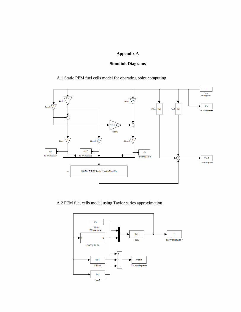
Appendix A

Simulink Diagrams

A.1 Static PEM fuel cells model for operating point computing

A.2 PEM fuel cells model using Taylor series approximation

58

A.3 Vehicle plant using PEM fuel cells subsystem

A.4 Taylor series approximation for vehicle plant using fuel cells

59

A.5 Top level vehicle harness

60

Appendix B

MATLAB Scripts

B.1 Script_Batt_Thev_AL.m

%% Script_Batt_Thev_AL.m simulates the nonlinear battery with Thevenin

Load close all; clear all; clc; StartTime = 0; StopTime = 30000; FixedStepSize = 1;

V2.time = [StartTime 20000]'; V2.signals.values = [3.25 3.2]';

for j = 1:20 tic; t_Thv_AL = sim('Batt_Thevenin_Load_AL'); toc; t(j) = toc; end;

AvgSimTime_Thv_AL = mean(t);

figure('Name','Nonlinear Battery Thevenin Load AL','NumberTitle','off')

subplot(1,3,1); plot(t_Thv_AL,Vbatt_Thv_AL); title('Voltage'); xlabel('t');ylabel('V','rotation',0); xlim([0,3e4]);ylim([3.18,3.36]); grid;

subplot(1,3,2); plot(t_Thv_AL,SOC_Thv_AL); title('State of Charge'); xlabel('t');ylabel('%','rotation',0); xlim([0,3e4]);ylim([0,80]); grid;

subplot(1,3,3); plot(t_Thv_AL,I_Thv_AL); title('Current'); xlabel('t');ylabel('A','rotation',0); xlim([0,3e4]);ylim([0,1]); grid;

save('Thv_AL.mat');

61

B.2 Script_Batt_Compare.m

%% Script_Batt_Compare.m compares the differences between battery

systems with and without memory block

load Thv_NoAL.mat; load Thv_Mem.mat;

Vbatt_diff = Vbatt_Thv_Mem - Vbatt_Thv_NoAL; SOC_diff = SOC_Thv_Mem - SOC_Thv_NoAL; I_diff = I_Thv_Mem - I_Thv_NoAL;

figure('Name','Compare Thevenin Load','NumberTitle','off')

subplot(1,3,1); plot(t_Thv_NoAL,Vbatt_diff,'linewidth',3); set(gca,'fontsize',14); title('Voltage'); xlabel('t');ylabel('V','rotation',0); % xlim([0,3e4]);ylim([3.18,3.36]); grid;

subplot(1,3,2); plot(t_Thv_NoAL,SOC_diff,'linewidth',3); set(gca,'fontsize',14); title('State of Charge'); xlabel('t');ylabel('%','rotation',0); % xlim([0,3e4]);ylim([0,80]); grid;

subplot(1,3,3); plot(t_Thv_NoAL,I_diff,'linewidth',3); set(gca,'fontsize',14); title('Current'); xlabel('t');ylabel('A','rotation',0); % xlim([0,3e4]);ylim([0,1]); grid;

B.3 Script_FuelCell.m

clc; close all; T = 343; F = 96485339; R = 8314.47; E0 = 0.6; N0 = 78; Kr = N0/4/F;

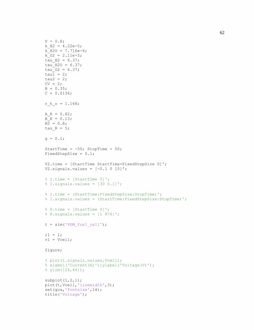
62

U = 0.8; k_H2 = 4.22e-5; k_H2O = 7.716e-6; k_O2 = 2.11e-5; tau_H2 = 6.37; tau_H2O = 6.37; tau_O2 = 6.37; tau1 = 2; tau2 = 2; CV = 2; B = 0.35; C = 0.0136;

r_h_o = 1.168;

A_R = 0.82; B_R = 0.13; R0 = 0.8; tau_R = 5;

g = 0.1;

StartTime = -50; StopTime = 50; FixedStepSize = 0.1;

V2.time = [StartTime StartTime+FixedStepSize 0]'; V2.signals.values = [-0.1 0 15]';

% I.time = [StartTime 0]'; % I.signals.values = [30 0.1]';

% I.time = (StartTime:FixedStepSize:StopTime)'; % I.signals.values = (StartTime:FixedStepSize:StopTime)';

% P.time = [StartTime 0]'; % P.signals.values = [1 876]';

t = sim('PEM_fuel_cell');

i1 = I; v1 = Vcell;

figure;

% plot(I.signals.values,Vcell); % xlabel('Current(A)');ylabel('Voltage(V)'); % ylim([24,44]);

subplot(1,2,1); plot(t,Vcell,'linewidth',3); set(gca,'fontsize',14); title('Voltage');

63

xlabel('Time(s)');ylabel('V','rotation',0); xlim([-10,50]); ylim([38.4,39.8]); grid on;

subplot(1,2,2); plot(t,I,'linewidth',3); set(gca,'fontsize',14); title('Current'); xlabel('Time(s)');ylabel('A','rotation',0); xlim([-10,50]); ylim([2.4,4]); grid on;

B.4 Script_Vehicle_AL.m

%% Script_Vehicle_AL.m simulates the vehicle model with algebraic loop % close all; % clear all; % clc; StartTime = 0; StopTime = 3000; FixedStepSize = 1;

T_req_AL.time = [StartTime 2000]'; T_req_AL.signals.values = [141.576 160]';

% for j = 1:10 % tic; t_EV_AL = sim('Vehicle_Plant_AL'); % toc; % t(j) = toc; % end;

% AvgSimTime_Vehicle_AL = mean(t);

figure('Name','Vehicle AL','NumberTitle','off')

subplot(2,2,1); plot(t_EV_AL,v_AL,'linewidth',3); set(gca,'fontsize',14); title('Vehicle Velocity'); xlabel('t');ylabel('m/s','rotation',0); % xlim([0,3e4]);ylim([3.18,3.36]); grid;

subplot(2,2,2); plot(t_EV_AL,SOC_AL,'linewidth',3); set(gca,'fontsize',14); title('State of Charge');

64

xlabel('t');ylabel('%','rotation',0); % xlim([0,3e4]);ylim([0,80]); grid;

subplot(2,2,3); plot(t_EV_AL,I_AL,'linewidth',3); set(gca,'fontsize',14); title('Current'); xlabel('t');ylabel('A','rotation',0); % xlim([0,3e4]);ylim([0,1]); grid;

subplot(2,2,4); plot(t_EV_AL,Vbatt_AL,'linewidth',3); set(gca,'fontsize',14); title('Battery Voltage'); xlabel('t');ylabel('V','rotation',0); % xlim([0,3e4]);ylim([0,1]); grid;

% save('Vehicle_AL.mat');