Embed Size (px)
Citation preview

MODELING AND OPTIMIZING ROUTE CHOICE FOR
MULTIMODAL TRANSPORTATION NETWORKS
Behzad Rouhieh
A Ph.D. Dissertation
in
the Department
of
Building, Civil and Environmental Engineering
Presented in Partial Fulfillment of the Requirements for
the Degree of Doctor of Philosophy (Civil Engineering) at
Concordia University
Montreal, Quebec, Canada
April 2016

ii

iii
ABSTRACT
Modeling and Optimizing Route Choice for Multimodal Transportation Networks
Behzad Rouhieh
Concordia University, 2016
Traffic congestion has been one of the major issues that most urban areas are facing and thus,
many solutions have been developed and deployed in order to mitigate its negative effects.
Advanced Traveler Information Systems (ATIS) have been used over the past two decades to
provide travelers with pre-trip or real-time traffic information. Most of the efforts have focused
on providing timely traffic information at locations with regularly occurring congestion. ATIS can
be used to provide travelers with pre-trip and on-route travel information necessary to improve
trip decision making with respect to various criteria (e.g. minimizing delay, constraining travel
to specific modes). Many jurisdictions within Canada and the United States have implemented
the 511 travel information system that provides traffic information, road conditions and
closures, traffic cameras, etc.
Several studies were conducted on vehicle routing optimization methods in ATIS. Most of them
consider passenger vehicles as the only transportation mode in their routing algorithm. Others
that include two transportation modes are mostly based on shortest path algorithms. However,
a probabilistic based route optimization approach could better capture the stochastic
characteristic of road traffic conditions. This research investigates an adaptive routing
methodology for multi-modal transportation networks. A routing algorithm based on Markov
decision processes is proposed to capture short-term traffic characteristics of transportation
networks. Graph theory is used to model typical travel behavior within a multimodal network.

iv
This thesis proposes to use special network modeling elements, e.g. super nodes, to allow the
integration of public transportation schedule into the model via the publicly available
predefined timetables. The proposed routing algorithm applies an iterative function to select
the optimal transportation mode/route through the network junctions along a given path.
The proposed methodology is applied to several real-world networks of motorized and non-
motorized modes located in the central business district in Toronto, Ontario, and Montreal and
Longueuil in Quebec. The networks include train, bus, streetcar, subway and bicycle
transportation facilities. Microsimulation models of the networks developed in VISSIM and
AIMSUN are used to estimate travel times along major arterials, for all transportation modes
and for different traffic demands and congestion levels. The simulation models were calibrated
using volume and speed data. The developed routing algorithm is applied to several scenarios
in order to estimate optimal routes for a hypothetical traveler moving between two arbitrarily
selected nodes in the network. The results identify the most efficient combination of
transportation modes that the travelers have to use given specific constraints pertaining to
traffic and transit service conditions. It is also shown that by applying the proposed algorithm to
bus lines, transit agencies can have significant cost savings by rerouting their fleet.
The results of the proposed research have the potential to be integrated into various Intelligent
Transportation Systems applications by combining available traveler information services. It can
assist travelers in making more informed decisions regarding their travel plans and provide
transportation agencies with an overall assessment of the system and its performance. For

v
example, it can be used to minimize the impact of congested traffic conditions on the overall
travel time and/or cost incurred by travelers as well as the operating cost of transit agencies.

vi
Acknowledgement
First and foremost, I would like to express my deepest gratitude to my supervisor, Dr. Ciprian
Alecsandru, for his continuous motivation, support and invaluable advice throughout my
studies. I also gratefully acknowledge my supervising committee: Dr. Saunier, Dr. Zayed, Dr. Li
and Dr. Hamza for their knowledgeable advice. This thesis owes an enormous debt to them due
to their professional and selflessness guidance.
I am proud to acknowledge that the support for this study was provided through the “Fonds
québécois de la recherche sur la nature et les technologies” scholarship no. 140734. I thankfully
acknowledge that a Paramics model with related traffic data was provided by Prof. Baher
Abdulhai of the University of Toronto for research use. I would like to thank Ministère des
Transports du Québec, Direction de l'Est-de-la-Montérégie for providing the traffic data and
signal timing plans.
I would like to extend my gratitude to my friends, colleagues at Concordia University
Transportation lab and CIMA consulting company: Matin Foomani, Siamak Sarhaddi, Reza
Omrani, Golnaz Ghafghazi, Pedram Izadpanah, Alireza Hadayeghi, Brian Malone, Chantal
Dagenais and Suzanne Demeules for their continuous support. Special thanks are due to Hamid,
Soraya and Shahrzad Mobasherfard for their unconditional support and encouragement.
I also want to express my deepest gratitude to my girlfriend Glareh Amirjamshidi who
supported me during the final, critical months of my dissertation, and made me feel like
anything was possible.
Last but not least, I wish to express my warmest appreciation and love to my wonderful
parents, Mahvash and Taghi and my trustworthy brother, Behnam and his kind wife Nikoo for
their continuous inspiration and support. I am indebted to their unconditional love and
encouragement.

vii
To my lovely parents and brother, this thesis is dedicated.

viii
TABLE OF CONTENTS
ABSTRACT ........................................................................................................................................ iii
TABLE OF CONTENTS..................................................................................................................... viii
LIST OF TABLES ................................................................................................................................ xi
LIST OF SYMBOLS ........................................................................................................................... xii
LIST OF ABBREVIATIONS ............................................................................................................... xiii
CHAPTER 1. INTRODUCTION ......................................................................................................... 1
1.1 Problem Statement .......................................................................................................... 1
1.2 Research Objective ........................................................................................................... 2
1.3 Research Methodology .................................................................................................... 3
1.4 Thesis Organization .......................................................................................................... 6
CHAPTER 2. LITERATURE REVIEW ................................................................................................. 7
2.1 Passenger Vehicle Routing ............................................................................................... 7
2.2 Transit Routing ............................................................................................................... 15
2.3 Multimodal Transportation Network Models ................................................................ 22
2.4 Route Choice Models for Transportation Networks ...................................................... 29
2.5 Application of Markov Analysis in Transportation ......................................................... 32
2.6 Traffic Conditions Prediction Models ............................................................................. 41
2.7 Concluding Remarks ....................................................................................................... 45
CHAPTER 3. METHODOLOGY ...................................................................................................... 48
3.1 Network Modeling ......................................................................................................... 49
3.2 Routing Algorithm Using Markov Decision Processes (MDP) ........................................ 54
3.3 Evaluation of Traffic Conditions and Transition Probability Matrix in MDP .................. 61
3.4 MDP Flowchart to identify Optimal Route ..................................................................... 62
3.5 Discussion on Transition Probability in Transportation Network .................................. 93
CHAPTER 4. ANALYSIS AND RESULTS ........................................................................................ 100
4.1 Montreal case study ..................................................................................................... 100
4.1.1 Analysis and Results .............................................................................................. 101

ix
4.1.2 Sensitivity Analysis ................................................................................................ 112
4.1.3 Discussion.............................................................................................................. 115
4.2 Toronto case study ....................................................................................................... 117
4.2.1 Network Model ..................................................................................................... 118
4.2.2 Model Calibration ................................................................................................. 123
4.2.3 Traffic Conditions and Transition Probabilities..................................................... 127
4.2.4 Public Transit Network .......................................................................................... 132
4.2.5 Routing Constraints............................................................................................... 135
4.2.6 Analysis Results ..................................................................................................... 135
4.2.7 Sensitivity Analysis ................................................................................................ 139
4.2.8 Discussion.............................................................................................................. 141
4.3 Longueuil case study .................................................................................................... 143
4.3.1 Model Calibration ................................................................................................. 146
4.3.2 Experimental Analysis ........................................................................................... 147
4.3.3 Computation Results ............................................................................................. 151
4.3.4 Sensitivity Analysis ................................................................................................ 155
4.3.5 Discussion.............................................................................................................. 157
CHAPTER 5. CONCLUSION AND RECOMMENDATIONS ............................................................ 158
5.1 Conclusion .................................................................................................................... 158
5.2 Major Contributions ..................................................................................................... 161
5.3 Research Limitations .................................................................................................... 163
5.4 Recommendation and Future Work ............................................................................ 164
5.4.1 Current study enhancement area ......................................................................... 164
5.4.2 Current study extension area ............................................................................... 165
PUBLICATIONS ................................................................................... Error! Bookmark not defined.
REFERENCES ................................................................................................................................ 167
APPENDIX A: AIMSUN Simulation Results .................................................................................. 178
APPENDIX B: Public Transit Schedule ......................................................................................... 185
APPENDIX C: Visual Basic Code for the MDP Algorithm ............................................................. 192

x
LIST OF FIGURES
Figure 1: Station nodes 𝒔𝟏, 𝒔𝟐 and their associated route nodes 𝒓𝟏, 𝒓𝟐, 𝒓𝟑, 𝒓𝟒 ........................ 53
Figure 2: Sequence of states, decisions, transitions and penalties for an MDP. .......................... 58
Figure 3: MDP Flowchart .............................................................................................................. 66
Figure 4: Example Network ........................................................................................................... 69
Figure 5: Time-Step Threshold Optimization Subroutine ............................................................. 96
Figure 6: Plan of study area (Source: Google Maps©) ............................................................... 102
Figure 7: Public transportation network within the study area (drawing not to scale) ............. 103
Figure 8: Modeled network (nodes/node), Montreal case study .............................................. 109
Figure 9: Travel time impact due to different probability values of service interruption at Metro
(Departure 4:00 pm) ................................................................................................................... 114
Figure 10: Travel time impact due to different probability values of bicycle unavailability and
different probability values of traffic congestion occurrence .................................................... 115
Figure 11: Layout of the study area, roadway network and select transportation modes (Source:
Google Earth) .............................................................................................................................. 117
Figure 12: Schematic model of the nodes/node numbers within the network ......................... 119
Figure 13: Schematic model of the links/link numbers within the network .............................. 120
Figure 14: GIS network acquired from LIO and the study area in this project ........................... 122
Figure 15: Study area modeled in AIMSUN ................................................................................ 122
Figure 16: GEH Statistics Calculations for the modeled study area ........................................... 126
Figure 17: Speed profile used for calibration – Gardiner Expressway ....................................... 127
Figure 18: Sample of 15-minute interval average speed profile along Dufferin St. (NB) ........... 128
Figure 19: Transit network within the study area ...................................................................... 134
Figure 20: Traveler’s optimal route ............................................................................................ 137
Figure 21: Second alternative route ........................................................................................... 138
Figure 22: Preferred route under normal traffic condition ........................................................ 139
Figure 23: Layout of Study Area (Source: Google Maps) ............................................................ 144
Figure 24: Alternative scenarios: lane closures in the network ................................................. 145
Figure 25: Bus routes: nodes and links ....................................................................................... 145
Figure 26: GEH Statistics Data ..................................................................................................... 147

xi
LIST OF TABLES
Table 1: Road Network Transition Probability Matrix (Montreal Case Study) ........................... 106
Table 2: Transition Probability Matrix for Metro Network ........................................................ 107
Table 3: Transition Probability Matrix for Bixi Network ............................................................. 107
Table 4: Sample route/station node parameters for metro and bus modes ............................. 110
Table 5: Estimated travel times for select modes from A to B – No Service interruption at metro
is expected (Departure at 4:00 pm) ............................................................................................ 111
Table 6: Estimated travel times for select modes from A to B – 20% chance of metro service
interruption (Departure at 4:00 pm) .......................................................................................... 112
Table 7: Estimated travel times (A to B) for different departure times ..................................... 113
Table 8: Transition Probability Matrix (Arterials) ....................................................................... 129
Table 9: Transition Probability Matrix (Highway) ....................................................................... 131
Table 10: Transition Probability Matrix (Study Network) ........................................................... 131
Table 11: Initial probability matrix when .................................................................................... 132
Table 12: Estimated travel times for select routes from A to B ................................................. 136
Table 13: Estimated travel times for select routes from A to B (revised transition probabilities)
..................................................................................................................................................... 139
Table 14: Estimated travel times for select routes from A to B (revised transition probabilities)
..................................................................................................................................................... 140
Table 15: Estimated travel times for select routes from A to B (Different transition probability
Matrices for arterials and highway) ............................................................................................ 141
Table 16: Vehicle input volumes ................................................................................................. 149
Table 17: Results of the t-test analysis for the travel time difference ....................................... 151
Table 18: Average travel time simulation results for select links (see Figure 25) ...................... 152
Table 19: Sample optimal routing results for the study network............................................... 154
Table 20: The effects of re-routing on trip cost-savings under different scenarios ................... 156

xii
LIST OF SYMBOLS
Symbol Description
𝑠𝑖 Transit Station 𝑖
𝑟𝑖 Transit Route number 𝑖
𝑧𝑖 Transit mode 𝑖
𝑡𝑟𝑧𝑖 Departure/Arrival time at route number r, for mode 𝑧𝑖
𝑤𝑟(𝜏) Link weight (travel time) on route r, at time t
𝑃𝑇 One-step transition probability matrix
𝑂 Origin node
𝐷 Destination node
N Number of nodes
𝐼 Number of states
𝑃(𝑛) State probability vector for the 𝑛𝑡ℎ node
𝑒(𝑛) Expected total penalties (travel time/cost) between node 𝑛 and
destination
𝑄𝑛+1(𝑛)
Matrix of penalties from node 𝑛 to 𝑛 + 1, in each possible state
R Route list to include all the interconnected nodes that build a route
between the origin and destination
Kn Set of directly connected (adjacent) nodes to node 𝑛
Mj Set of transportation modes related to each node in R
𝑅𝑜𝑝𝑡 Optimal route
𝐸𝑚𝑖𝑛 Expected minimum penalty for the optimal route
𝑇𝑡𝑟 Time-step threshold

xiii
LIST OF ABBREVIATIONS
Abbreviation Description
AMT Agence Métropolitaine de Transport
APTS Advanced Public Transit Systems
ATIS Advanced Traveler Information Systems
CBD Central Business District
EB East Bound
GTA Greater Toronto Area
ITS Intelligent Transportation Systems
MDP Markov Decision Process
MTO Ministry of Transportation Ontario
MTQ Ministry of Transportation Quebec
NB North Bound
RTL Réseau de transport de Longueuil
SB South Bound
STM Société de Transport de Montréal
TTC Toronto Transit Commission
VB Visual Basic
WB West Bound

1
CHAPTER 1. INTRODUCTION
Deployment of Intelligent Transportation Systems (ITS) improves the performance of the
transportation system by using modern electronics and communications technologies.
Advanced Traveler Information System (ATIS) and Advanced Public Transit Systems (APTS) are
two types of ITS user services that aim to ameliorate traffic operations on urban transportation
networks. The benefits of ATIS and APTS implementation are more evident under congested
traffic conditions, either recurrent (due to morning and afternoon peak travel demand periods)
or non-recurrent (e.g. due to incidents that hinder available road capacity).
1.1 Problem Statement
Several studies have shown the benefits of using various ATIS and/or APTS applications to
reduce traffic congestion, economic productivity loss and greenhouse gas emissions. Currently,
several Canadian agencies have deployed different ITS applications available to the travelling
public. For example, up-to-date information about highways is accessible via phone or a
dedicated website for several provinces, e.g. 511 Traveler Information Center in Nova Scotia
(Road Conditions 511, 2012) and Quebec (Quebec 511, 2012). Moreover, many travel operators
provide real time schedule of their services. However, corroborating road traffic conditions with
public transportation services and other non-motorized transportation modes information is
expected to further enhance the traveling experience by providing more efficient and reliable
transportation services. Within large urban agglomerations, this is expected to be beneficial for
both the traveling public and transportation operators.

2
ATIS/APTS can be used to provide travelers with pre-trip and/or on-route information
concerning traffic conditions, travel options as well as real-time advice on navigating through
the transportation network, where travel conditions may change rapidly several times during
the course of a typical day. The major benefits of this type of ITS applications, as shown in
several studies, are the expected reduction in travel time delay, typically obtained by providing
optimal route information. Mostly, this is done based on the online data made available at any
time to the travelers who want to plan or make necessary adjustments to minimize their trip
travel times. Moreover, transit operators would benefit by managing their fleet more efficiently
and by providing passengers with more reliable services. For example, in case of incidents that
cause severe traffic congestion, a transit agency would be able to minimize the disruption to
the original timetable and reduce the impact on the operating costs by rerouting buses at
certain nodes using real-time information about traffic conditions. This research proposes a
novel and versatile methodology to provide adaptive routing in multimodal transportation
networks. The proposed methodology is applied to real-world test cases to validate its
effectiveness.
1.2 Research Objectives
The main objectives of the research presented in this dissertation are:
[1] to advance a novel routing methodology based on graph theory;
[2] to integrate different transportation modes into the methodology;
[3] to demonstrate that the proposed methodology is able to realistically capture the
stochastic effects of traffic conditions within a multimodal transportation network; and

3
[4] to identify the optimum route within a multi-modal transportation network. This can be
achieved by targeting a specific optimization criterion. For example, one may use the
proposed modeling approach in order to minimize the impact of congested traffic
conditions on the overall travel time and/or cost for travelers and/or transit agencies.
1.3 Research Methodology
The proposed methodology uses a routing algorithm implemented based on a Markov Chain
with Reward model. The optimization criterion used by the developed algorithm seeks to
minimize the negative impact of congested traffic conditions on users’ routing. Several real-
world case studies are tested to demonstrate the feasibility of the proposed method. To
achieve the proposed objectives, the following tasks have been conducted:
1. Defining a generic representation of each physical transportation network
corresponding to different transportation modes (i.e. road, transit and rail). Since public
transportation services operate based on a predefined schedule, in order to be able to
realistically integrate this type of networks, the developed model accounts for the fixed
schedule of public transportation services as well as stochastic variability of the
observed travel times.
2. Collecting and processing transportation related data from several sources (e.g.
provincial and municipal transportation authorities, etc.) to integrate in the
transportation network model. In this task, several traffic data and information sources
were considered depending on the location and the type of the transportation networks
used. A set of stochastic properties pertaining to the study networks were investigated

4
- including short-term fluctuation of travel demand, transit schedule and non-recurrent
congestions along major arterials. Traffic data (e.g. speed, travel time, etc.) were
obtained from transit authorities/agencies.
We have acquired traffic data from the Ministry of Transportation of Quebec. The
schedule of the transit services was collected from the Agence Métropolitaine de
Transport (AMT), the Société de Transport de Montréal (STM) and Toronto Transit
Commission (TTC). Additional information about the bicycle sharing services (i.e. BIXI in
Montreal and Bike Share in Toronto) was obtained from the transportation departments
of Montréal and Toronto. A database was developed in Excel to provide concurrent
access to the collected data.
3. Developing and calibrating microscopic simulation models in Vissim and Aimsun to
estimate travel times for major arterials and all transportation modes under several
traffic demand and congestion scenarios. The results were used to emulate the lack of
available historical traffic data of the real-world transportation networks used in this
thesis to test the route optimization algorithm.
4. Developing an optimal route algorithm that can be used in user equilibrium and system
optimal models. The proposed algorithm integrates the time and/or cost (of the trip)
constraint into a single performance measure. The algorithm was validated with
historical and real-time information about travel conditions in a stochastic and time
dependent modeling approach.
5. Developing a traffic state prediction model to better capture the stochastic behavior of
transportation networks. The applied methodology uses changes in traffic speed as the

5
traffic condition indicator to predict congestion level. The results were used to estimate
the transition probabilities of Markov Chain model.
6. Applying the proposed methodology to several real-world transportation networks to
identify the benefits of developed a routing algorithm. The studied transit network was
chosen to investigate the application of the proposed method in on-demand transit re-
routing for transportation agencies (e.g. bus line alignment changes with the network
traffic). In addition, multimodal networks were built to study travelers’ optimized
routing in transit networks in case of congestion or unforeseen delays.
The main thesis contributions are as follows:
This thesis presents a new approach in developing an ITS methodology by combining available
services and providing an integrated public and roadway traffic application. Previous route
optimization studies consider passenger vehicles as the only transportation mode in their
routing algorithm. In this research, a methodology is developed to use Markov process in route
optimization algorithm for a multi-modal transportation network. The proposed approach
applies probabilistic based methods to better estimate the parameters related to the stochastic
nature of traffic parameters in a transportation network.
The proposed route optimization model can benefit various stakeholders, particularly transit
operators and users, local transit agencies that provide feeder bus services to regional bus
passengers to commute within the suburban communities, government agencies and industries
related to the ITS. This methodology can be integrated into end-user products that would be
beneficial for both travelers and transportation service providers.
6
For example, transit users would be able to modify their plans and choose other modes of
transportation if the current mode experiences delays due to traffic conditions. In regards to
transit operators, the proposed method enables them to share information on several transit
services and stops/stations and reduce passengers’ wait time and/or transit delay costs, assist
planners in revising transit schedules periodically and provide real-time routing guidance to bus
drivers.
1.4 Thesis Organization
Chapter 2 presents a literature review on the existing methods adopted by authorities and
researched by academics for route optimization in transportation networks. The different
approaches are discussed and investigated. Limitations and gaps in each approach are
presented. Chapter 3 includes the development of the proposed methodology. It starts by
developing the optimization methodology based on Markov Decision Process, followed by the
traffic state prediction methodology. In addition, it includes a flowchart explaining the
implementation of the proposed methodology. An example is presented to demonstrate the
application of the proposed methodology in a small network. The chapter concludes with a
discussion on improving the state transition probabilities used within a network. Chapter 4
presents three case studies developed to validate and implement the proposed methodology
and prove its application in transportation networks. It also includes the data collection stage,
which is an integral part of the research and model development. Finally, Chapter 5 summarizes
the research and presents the thesis contributions and identifies future work directions.

7
CHAPTER 2. LITERATURE REVIEW
Given that traffic conditions on real-world transportation networks show stochastic and time
dependent properties (e.g. occurrence and duration of non-recurrent congested conditions,
fluctuations in demand for transit usage, etc.) transportation operators and passengers can
benefit from deployment of ITS applications such as Advanced Traveler Information System
(ATIS) and Advanced Public Transit Systems (APTS). By providing travelers with updated travel
time/route information, they will be able to make more informed route choice decisions,
mainly to minimize travel delay. ITS deployments provide benefits to the public transportation
operators. By incorporating adequate online information, transit authorities will be able to
adjust the operations of their fleet to respond more efficiently to various conditions hindering
normal operation and, consequently, minimize the negative effects on passengers’ travel time.
An overview of recent studies on the vehicle routing is performed and categorized as described
here after.
2.1 Passenger Vehicle Routing
In recent years, many studies investigated different network assignment and vehicle routing
algorithms and related ATIS applications. ATIS is intended to improve traveler decision making
by collecting, processing and disseminating information that helps travelers decide when to
travel, the mode to choose and the route to take. For example, Huang and Li (2007) presented
a traffic equilibrium model to evaluate the effect of ATIS as a travel information service on
travel behavior. Their multi-criteria, logit-based model used a trade-off between travel time
and travel cost to make route choices based on the value of time for different users. The
authors assumed that all users select the routes with minimum perceived travel disutility, which

8
is a linear bi-criteria combination of travel time and monetary travel cost. Two types of users
were studied: equipped and non-equipped with ATIS. The authors found that their model had a
better estimation of network benefits of ATIS compared to other single-criterion models (i.e.
travel time-based or travel cost-based single-criterion models).
Other studies had investigated travel time prediction under ATIS. For example, Abdalla and
Abdel-Aty (2006) studied the benefits of ATIS in route choice at microscopic level. The authors
used a mixed linear modeling approach to study travel time under ATIS. They used a real world
network with 40 links and 25 nodes, and vehicle flows in a travel simulator, where a traveler
drives in a simulated environment, to generate dynamic route choice data. Travelers were
provided with one of five different levels of information and/or advice, including no
information, pre-trip/on-route information with/without advice. The authors analyzed travel
time of total of 630 trial trips completed by the 63 travelers. The authors’ study focused only on
drivers using passenger cars and concluded that by increasing the level of information (i.e.
adding on-route knowledge to pre-trip information) the average travel time decreased.
Bingfeng et al. (2008) presented a bi-level programming model to determine the optimal
system performance of traffic network within an ATIS environment. In their model traffic
authority is the decision maker in the upper-level problem, and drivers - with or without ATIS,
are the decision makers in the lower-level problem. They used a numerical example to
demonstrate the application of model and investigated the traffic behaviors under three cases
of the ATIS environment: (i) ATIS provides drivers with parking and route information, (ii) ATIS
provides drivers with route information only, and (iii) ATIS provides drivers with parking

9
information only. Their findings showed that ATIS with parking information would be most
effective when parking demand is reaching capacity, and the roads are not congested.
Yang and Luk (2008) studied the impact of ATIS on the performance of road network. The
authors used traffic simulation module to represent the traffic and calculate network delay as
the main performance measure. They considered four categories of drivers, based on the level
of access to traffic information. The route choice model proposed by the authors categorized
drivers into four groups, drivers with i) no traffic information; ii) pre-trip information; iii) real-
time traffic information; and iv) displaying messages using variable message sign, respectively.
The method was applied to a case study in Singapore consists of express ways and arterials. The
authors also conducted an analysis of different percentage of market penetration (i.e.
percentage of travelers that have access to driving information system). Their results showed
that providing traffic information to drivers can reduce the total network delay by 7.5%. In
addition, they found the optimal level of market penetration for each demand, which would
result in the performance of a real-time information system to be better than or equal to that
of the pre-trip system. Their results were mainly based on simulation and were not validated
with real world data.
Another category of studies are those that evaluated different route choice techniques. The
reviewed literature shows that most discrete choice models for route choice analysis are based
on static and deterministic networks. Examples of such models are Path Size Logit (Ben-Akiva
and Ramming, 1998; Ben-Akiva and Bierlaire, 1999) and C-Logit (Cascetta et al., 1996). These
models are non-adaptive path choice models because travelers are not allowed to adjust their
10
route choices on-route in response to the revealed traffic conditions. Several studies of path
choice models with real-time information, both pre-trip and on-route, and a recent related
literature review can be found in Abdel-Aty and Abdalla (2006).
Some models investigate drivers’ behavior to predict the decision to switch from a previously
chosen or experienced route and others are route choice models with explicit choice sets of
paths. For example, Srinivasan and Mahmassani (2003) studied the effect of observed
heterogeneity due to age and gender effects in user decisions under real-time information.
Abdel-Aty and Abdalla (2004) investigated drivers’ diversion from their normal routes under
different scenarios of providing traffic information (i.e. no information, pre-trip information
without and with advice, and on-route information without and with advice). Their study
network was located in the area around the University of Central Florida and included 25 nodes
and 40 links. In total 630 trial trips by 63 drivers were studied. Their results showed that the
travel time of the normal and diverted routes are significant in encouraging drivers to divert
from normal routes. Also it was shown that expressway users may divert from the expressway if
they are guided to a route with a temporarily less travel time. Bogers et al. (2005) investigated
learning, risk attitude under uncertainty, habit and the impacts of advanced travel information
service on route choice behavior. The authors developed a conceptual framework to integrate
these aspects and used the interactive travel simulator of Delft University of Technology (TSL)
to investigate route choice among a given number of paths for travelers. They concluded that
people perform best under the most elaborate information scenario and that habit with on-
route information plays a major role in route choice behaviors.

11
Ukkusuri and Patil (2007) developed a methodology for traffic assignment by accounting for
travelers’ recourse actions (opportunity for the traveler to evaluate his or her remaining path
when en-route information is available). They applied a methodology based on Logit model and
Hyperpaths (i.e. subset of links connecting adjacent nodes with different probabilities). The
authors’ methodology includes a utility function based on minimizing the total cost of traveling
between the origin and destination nodes. In their model the link cost is a function of traffic
flow and has to be recalculated for all the links in each iteration. An iterative stochastic user
equilibrium approach is utilized to find the most efficient Hyperpath (minimum cost). The
authors applied the proposed method to a test network and achieved convergence in less than
100 iterations. They concluded that the methodology could be efficiently adopted for stochastic
user equilibrium with recourse.
Some studies proposed various algorithms to solve different routing policy problems. For
example, Gao and Chabini (2006) studied the optimal routing policy (ORP) problem in stochastic
networks. The authors reviewed different variations of optimal routing policy problem in the
literature. They implemented an ORP algorithm that accounts for stochastic dependency among
link travel times and they investigated the role of information in routing decision making. Gao
et al. (2008) presented a route choice model to capture travelers’ behavior when adapting to
the provided traffic conditions en-route, in a stochastic network. The authors proposed a
routing policy to represent drivers’ adaptive behavior. Their routing policy is defined as a
decision rule that maps all possible traffic conditions to the next links at a decision node (e.g.
Choosing the route between the two traveling points with minimum travel delay). A variable
message sign was used to provide information about congestion status on the network links.

12
Their findings showed that between the routing policy model and the non-adaptive path model,
where traveler cannot change their path while on-route, there is a significant difference in
terms of expected travel time, when the network is more unpredictable (i.e. the probability of
an incident is in the medium range).
Nikolova and Karger (2008) presented an optimal solution approach to find an optimal policy
that minimized the expected cost of travel for the Canadian Traveler problem. The Canadian
traveler problem is a stochastic shortest path problem in which travelers learn the cost of a link
only when they arrive at its connecting junction. The authors applied a mix of techniques from
algorithm analysis and the theory of Markov Decision Processes to develop algorithms for
directed acyclic graphs. The proposed solution was not validated for other types of graphs.
Other studies investigated in-vehicle routing solutions by using real-time information. For
example, Du et al. (2013) proposed a coordinated online in-vehicle routing mechanism for
smart vehicles with real-time information exchange and portable computation capabilities. This
study considered that at a given short time period, there was a group of smart vehicles which
need to make route choice decisions among a number of candidate routes, according to the
latest real-time traffic information. The authors proposed a coordinated online in-vehicle
routing mechanism and modeled it as a mixed strategy routing game, in which the process that
smart vehicles decided their own route choice priorities was treated as a negotiation and
coordination process among other smart vehicles. In a routing coordination group, each smart
vehicle was seeking to find the best online route choice priority, which leads to the probabilities
of choosing the candidate paths with minimum expected travel time. The coordinated vehicles

13
iteratively updated and proposed their routing choice priority in responding to their evaluation
of near future traffic condition based on shared online traffic information. The negotiation
process repeated several iterations until all travelers accepted and would not change their
route choice priorities (i.e. an equilibrium route choice priority decision). The transportation
network is represented by a directed graph. At each iteration individual vehicle predicted the
expected traffic flow based on the latest traffic flow information and other vehicles’ route
choice proposals. When new traffic condition becomes available, each smart vehicle computes
its new targeting route choice priority through a multinomial logit choice model. The utility
function of the model was expected travel time on each path during current iteration. The
process of updating traffic condition and proposing new route choice process was repeated
until the targeted route distribution was the same as the current route choice priority for all the
vehicles (equilibrium routing decision). Authors conducted numerical experiments to
demonstrate the performance of their proposed routing mechanism by modeling a sample
network of Sioux Falls City. The results showed that by increasing the percentage of smart
vehicles, the ratio of average travel times between the proposed and traditional methods
became smaller, which indicated shorter travel times under the coordinated routing method. In
addition, the authors showed that their method outperformed the traditional routing method,
in which each smart vehicle decides its route choice priority independently without
coordination.
In another recent study Xiao and Lo (2014) proposed an in-vehicle navigation algorithm based
on adaptive control. The proposed algorithm incorporates historical traffic information to
minimize the expected on-route travel time. The transportation network is divided into a finite

14
number of nodes or decision points (e.g. intersection) and links (e.g. arterials). The authors
assumed a different traffic state at each node and formulated the travel time between two
nodes as a function of estimated travel time on the link between two nodes and the
uncertainty between actual and estimated travel time. The traffic states were defined as factors
that will influence the uncertainty of travel time (e.g. traffic signal) and the travel time was
calculated by applying the traffic state vector and the probability of occurrence of each traffic
state to the estimated travel times. Ultimately, a cumulative expected travel time from origin to
destination was defined and minimized to identify the optimal routing policy. The proposed
optimization did not produce a predetermined route for the vehicle. Instead, the next direction
to be taken was a function of the arrival state at a node. Therefore, the decision rule was
adaptive to the most recent traffic states encountered. The author then compared their
methodology with a deterministic algorithm that calculated an instantaneous shortest path and
showed that the adaptive routing policy outperformed the instantaneous shortest path
algorithm through an example network. Their results showed that, for most of the links, the
average path travel times of the proposed routing policy were between 1% and 7% shorter than
those of the time-dependent instantaneous shortest paths, particularly when the traffic volume
was high. The main limitation of this study is the assumption of conditioning factors that
influence traffic state and the variability in travel time. These factors need to be calibrated
based on historical data or through several scenarios within simulation models. A more realistic
approach to estimate the probability of traffic states should be used. In addition, the authors
only considered one single mode (private cars) in their methodology.

15
The above studies reveal different vehicle routing optimization methods in ATIS. However, they
only consider a single transportation mode (i.e. passenger vehicles) in their routing algorithm,
while many commuters of large urban agglomerations often times used a combination of at
least two transportation modes. This research work includes both private and transit modes in
optimal travel route calculations. This approach would enable both travelers and transit
agencies to benefit a multi-modal route optimization.
2.2 Transit Routing
There are a few studies about dynamic routing in transit networks. Jeremy and Mathew (2011)
developed an optimization method for bus transit system design using intelligent agent
architecture, which allows for more efficient evaluation of trade-offs between passenger cost
and operator cost. The authors applied their method to transit networks in Switzerland and
India, which were previously investigated. According to the authors, for both networks the
agent optimization system improved on the best of the previous solutions, both in terms of
operator cost and passenger utility. Wang et al. (2009) presented a simulation-based
optimization method for campus bus routing. The objective of their study was to find the
minimum-cost route, while minimizing each passenger’s inconvenience by satisfying their
request (fewer complains). The authors used numerical experiments to validate their proposed
simulation model. The method was applied to a High-Tech zone in Dalian city in China. The
authors conducted a numerical experiment based on the real data from a university campus
bus service to evaluate the validity of their proposed model. Their new vehicle routing
methodology was tested to divert a bus away from its fixed route in response to a new
16
customer request and was found to be beneficial to high-tech zone campus bus managers by
reducing their costs.
Fu and Lam (2014) presented an activity-based network equilibrium model for scheduling daily
activity travel patterns in transit networks under uncertainty. The authors uses supernetwork to
simultaneously consider individuals’ activity and travel choices (i.e. time and space
coordination, activity location, activity sequence and duration, and route/mode choices). They
assumed the activity utilities to be time-dependent and stochastic in relation to the activity
types and modeled activities with different durations or different start times as different
activity links. The authors proposed a route searching algorithm based on method of successive
average to solve for equilibrium. The objective was to maximize a daily activity utility function
by considering value of time and link travel costs. The studied network consisted of one subway
line and two bus lines. The results of their study showed that individuals’ travel choices were
affected by travel dis-utilities of different transit lines. For example, when the network was not
congested (i.e. low population), the dis-utilities of different transit lines were all quite small and
therefore, the percentages of people choosing different lines are almost equal. As the
population increased, they found a significant difference between the demands for two bus
lines until the network became extremely congested where the individuals had little preference
towards two bus lines. This network only included transit (not road network). The authors used
a very small network to apply their proposed methodology and their results were not calibrated
with real data. Moreover, the effect of road congestion and variations in travel times was not
considered in the analysis.

17
Crainic et al. (2008) used a demand adaptive model to capture the behavior of transit systems
with mandatory and optional stops (i.e stops requested by passengers and that may lead to
changes in the default bus route). The authors suggested that a master schedule has to be
developed based on time windows associated with mandatory stops. The authors employed a
particular sampling technique to solve a master schedule problem for a single bus line. The
efficiency of the proposed methodology was tested using various lengths and scenarios of the
hypothetical transit line.
In a different study, Panou (2012) investigated the optimization of public transport (PT)
information services that are provided on mobile devices, for travelers of PT means, through
their personalization. The author proposed an algorithm along with the necessary parameters
(dynamic and semi-dynamic) that supported a holistic personalization, based on each user
specific profile and the history of their previous selections. The dynamic parameters were
calculated automatically by the system and included: Walking distance, preferred transit mode,
Number of changes between transport modes, distance and cost of each route. Semi-dynamic
parameter was chosen each time the traveler used the application and included the reason for
travelling (Tourist, Commuter, Recreational or Emergency). During the learning process of user
preferences, the selected parameters were monitored and the corresponding values were
stored based on the selected route, each time the user makes use of the system. The history of
user preferences was used for future route recommendations. The author tested the proposed
model with 10 users and evaluated its performance by providing users with a questionnaire and
asking for their feedback. By using an average scoring value for the questions, the author
concluded that the users had a positive opinion for the application of personalized routes
18
provided. This study showed the possibility of providing beneficial information about travelers
routes/modes via mobile tools. However, only the scheduled travel time of transit modes are
used for analysis.
Lin and Bertini (2004) proposed a Markov chain model for bus arrival time prediction that
captures the behavior of bus operators in putting delayed or ahead of schedule buses back on
their predefined schedule. They used a link-node representation of the bus network. The
proposed methodology is demonstrated for a hypothetical case of equally spaced bus stops and
a possible solution for more realistic bus lines is discussed. They suggested using three
performance measures to evaluate the effectiveness of their prediction algorithm: overall
performance (minimum total prediction error), robustness (minimize the occurrence of large
deviations) and Stability (prediction of travel time does not fluctuate from time to time). The
transition probability in the proposed model represented the conditional probability of a bus
being delayed at downstream stop, given the delay at current stop. The authors suggested
integrating the proposed model to a bus arrival prediction algorithm. There are several
limitation in this study. The authors assumed that bus tops are uniformly spaced. The
effectiveness of this algorithm was not tested with actual data from transit operators.
Moreover, the authors did not use real data to calibrate their transition probability matrix.
In another study, Wong (2009) developed a dynamic mathematical model to estimate regional
bus journey time using Artificial Neural Networks (ANN). The model updates bus arrival time
using real-time Global Positioning System (GPS) information and also real-time highway loop
detector data of volume, speed and occupancy. The ANN model was used for predicting arrival

19
time of one bus route within Toronto and was compared to two other forecasting methods,
historical average and linear regression, and outperformed them by an average of 35 and 26
seconds in travel time calculations respectively. The author reports overestimation of arrival
time in their model, which could result in passengers missing the bus. This study only predicts
the bus travel time travelling mainly along EB direction of Gardiner Expressway in Toronto and
does not consider other bus lines travelling on parallel arterials. Also, due to limited available
data, the time period used in this covers only morning period: 5:30 till noon and does not
consider Toronto’s rush hour traffic during PM peak.
Polyviou (2011) proposed a simulation-based model capable of modeling the details of bus and
traffic incidents (SIBUFEM) in order to assess the impact of incidents on overall bus
performance and suggest potential fleet management strategies for improved efficiency. The
author considered three key performance measures to evaluate the effect of incidents: (i)
average bus journey time, (ii) average bus speed and (iii) average excess waiting time. The
author used data from the Portswood corridor bus route in Southampton, UK to calibrate and
test the model. The results showed that the higher the severity (capacity reduction) of a traffic
incident, the higher is the expected impact of the event on the overall bus performance. Their
finding showed that 25% and 40% reduction of capacity caused 0.25 and 0.54 minutes average
increase in travel time respectively. Also, the author concluded that a longer duration of a
traffic incident causes more severe effects on the overall bus performance: i.e. similar incidents
lasting for 20, 40 or 60 minutes, caused 0.1%, 1.3% and 2.8% increase in the average bus travel
time. The authors suggested that the travel time results of SIBUFEM could be used for further
evaluation of the impact of the incidents on bus patronage (ridership) levels. This study

20
quantifies the expected delay for one bus line during limited number of scenarios however, it
does not provide any re-routing solution via alternative route. Moreover, There are other
limitations in the simulation model: the computer model was not calibrated for vehicular traffic
and the traffic signals were not coded and their effect was replaced by an additional delay. In
addition, the severity of incidents is coded as a reduction in the road capacity, while a
microsimulation model that simulates different lane closures and interactions between vehicles
trying to change lane, could provide better and more realistic results.
Wang and Cheng (2012) proposed an allocation method for increasing the Public Transit (PT)
level of service in an urban network. Their proposed method is based on Hub-Spoke structure
that integrates PT lines with transfer hubs. Their approach focused on planning bus rapid
transport (BRT) and regular bus lines. The authors did not include other transit modes (e.g.
subway) nor transfer hubs (i.e. terminals or transfer stations) in the optimization process. They
used an objective function for BRT line to maximize the operating efficiency (ratio of passenger
person kilometers to total kilometers traveled by all buses over a day) within the network.
Similarly, for bus lines, their objective function was to maximize the density of nonstop
passenger volume (the ratio of the nonstop passenger volume of the bus line divided by the
length, i.e. distance, of the bus line). Nonstop passenger was referred to a traveler who would
not get off the bus until the final stop. They applied the proposed method to a PT network with
16 Traffic Analysis Zone (TAZ) in the City of Fuzhou in China. Operating efficiencies of feasible
bus lines between two transfer hubs were calculated and the path with maximum efficiency
was selected as the optimal BRT/bus line for that path. The authors proposed their
methodology could be used in PT line planning. This study has some limitations. The solution

21
method and the constraints used for the analysis need validation. Any modification to the
network size has a large effect on the solution time.
Other studies have addressed public transit schedule reliability and system efficiency issues.
For example, Teklu et al. (2007) evaluated the transit assignment of systems characterized by
small capacity buses (12-20 passengers) and stochastic headways (no timetables). Particularly,
the authors proposed a composite frequency-based and schedule-based Markov process model
for capacity constraint transit networks. Their model included bus and passengers’ simulator
and a random utility model for transit route choice. Their approach assumed passengers’ routes
were defined by a sequence of transfer stops connected by alternative route-sections to
represent the attractive lines passengers could choose to travel on. Their generalized cost
function consisted of in-vehicle travel cost, waiting cost and transit fares. A multinomial Probit
route choice model that considers the cost correlations between alternative routes was used to
model passengers route choice. The authors applied their model to a small network with 4 bus
stops and 2 bus lines. Their results showed that passengers on relatively congested sections of
the network experienced higher cost variability, due to the additional stochasticity associated
with finding spare seats in the buses. The authors concluded that their model could be applied
for network where transit vehicles are small and not operating to timetables to represent the
variability in flows and costs and enable planners make more informed decisions.
The above literature shows applications of route choice models in evaluation of performance
and schedule reliability and estimation of arrival time in public transit network. These studies
mainly consider one transit mode models which can be further developed by including other
22
transportation modes (i.e. private and other public transit modes). By including several transit
modes, travelers would be able to modify their plans and choose other modes of transportation
if their current mode experiences delays due to traffic conditions. Moreover, commuters using
their own vehicles could have a better planning for their trips if the option of switching
between car and transit is available to them.
2.3 Multimodal Transportation Network Models
Multimodal transportation involves the usage of at least two modes of transportation to
complete a single trip. Common modes of urban transport today mainly include car, bus, rail,
motorcycle, bicycle and walking. Multimodal networks inherently offer redundancy and
flexibility by offering multiple choices and routes, while mitigating the negative effects of traffic
congestion. On the other hand, transfers between different modes carry a certain overhead in
terms of waiting time and convenience and sometimes are a key factor in the decision of
making a specific multimodal trip. Modeling multimodal transport requires identifying the
availability of various transportation modes at specific locations and the ability and reliability of
transfers between these different modes.
A limited number of studies attempted to model multimodal transportation networks that
include both private and public transportation vehicles. Nagurney and Smith (2003) proposed
to represent this type of networks as a supernetwork. Supernetwork framework allows one to
formalize the alternatives available to decision-makers, to model their individual behavior and
to compute the flows on the supernetwork, which may consist of travelers between origins and
destinations as well as the associated costs. The supernetwork has the advantage that it can

23
model simultaneously multiple physical networks while accounting simultaneously for different
trip features (e.g. route choice, transfer/waiting time, cost of transfers, etc.). The authors
presented an overview of development and application of the supernetwork concept in
transportation and decision-making concepts. The authors did not provide any specific case
study or real world example of such modeling approach.
Zhang et al. (2011) presented a generic multimodal transportation network model for ATIS
application to be used for large-scale transportation systems. The authors proposed using a
supernetwork framework that integrates individual networks representing different
transportation modes. Their model included dynamic travel times and timetable of public
transportation services. The authors used the basic Dijkstra algorithm for routing purposes and
they used the travel time as the performance measure for best route choice. Their results
indicated that the model could be used to find optimal routes in short computation time for
realistic networks. The main limitation of their model was long computation time to read and
compile the integrated network, which depending on the size of network may take several
hours.
Casey et al. (2013) presented an analysis of the computational performance of two shortest
path algorithms for a multimodal multiobjective trip planner tool. The authors used Graph
theory to create the road and public transport networks where a set of nodes and links that
connect neighboring nodes together. They compared the performance of two shortest path
algorithms: simple Dijkstra and A* heuristic, which improves upon Dijkstra’s algorithm.
Dijkstra’s algorithm only considers the cost to travel from the origin node to the candidate

24
nodes and sorts candidate nodes in the order of their cost from the origin node. However, the
A* heuristic method estimates of the cost to travel from the candidate node to the destination
node, plus the calculated cost from the origin node to the candidate node, and orders the
nodes based on total origin-destination cost. They applied the proposed methodology to an
area of suburbs (as origins) and major destinations (e.g. CBD and airport) in the South East
Queensland region in Australia. A set of constraints were set for the analysis which included:
maximum number of transfers and maximum walking/transfer distance. The travel time value
was used as the performance measure. The authors concluded for road only network, A*
outperformed Dijkstra’s algorithm while for public transport and/or multimodal networks,
using Dijkstra as the shortest-path algorithm produces adequate results, with the average
search completing within 5-10 seconds compared to minimum 15 seconds in the A* method.
This study did not include any real time information and cannot be implemented in time
dependent networks.
Meng et al. (2014) presented a dynamic traffic assignment model for urban multi-modal
transportation network by constructing a mesoscopic simulation model. The authors used
MesoTS simulation laboratory previously developed by Yang (1997). The proposed model
updates the path travel time at the beginning of each iterative phase, finds the shortest path
with the k-shortest path algorithm, and finally assigns the traffic flow based on a C-Logit model.
Travel utility function was used to calculate the updated link travel times at the beginning of
each iteration. The k-shortest path algorithm is an extension of the typical Dijkstra algorithm
with the possibility to calculate a set of shortest travel time paths, and determine the distinct
set of the shortest path numbers according to different criteria. The authors applied their

25
proposed model to an area in the Chaoyang district in Beijing. The network consists of 5 subway
lines with 39 stations, 18 bus lines with 51 stations and 188 road links with 122 nodes. The
authors conducted several experiments to study the effect of different factors (e.g. increase in
demand, parking fees and car ownership) on the percentage of car and transit (bus/subway)
travel trips. In one of the conducted experiments, they examined the effect of traffic
information on the travel mode choice. The results showed that when the car transfer
information was not provided, (drivers had no opportunity to transfer to other modes) the
private car trip increased from 61.5% to 86.5%. Similarly, when the transit transfer information
was not provided, the one transit line trip increased from 3.9% to 6.2% (lower number of mode
changes due to lack of transfer information). In both cases the average travel time increased by
1-2%. Finally, when no transfer information was provided, most of the travelers chose the
private car trip, and the average travel time increased as the traffic congestion aggravates.
Authors reported slow computation process for the time-dependent shortest path algorithm. In
addition, this methodology does not account for real-time traffic information and changes in
traffic conditions.
Arentze and Timmermans (2004) developed a network representation of multimodal
transportation systems that allows the modeling of multi-activity, multimode routes by means
of a standard least-cost path finding method. A case study was tested along the Almere–
Amsterdam corridor in the Netherlands. The purpose of their study was to assess the
sensitivity of activity-travel choice behavior on the travel time and cost from Almere to
Amesterdam. The authors implemented a two-activity program (working and shopping) under
various specifications of cost functions (e.g. value of time, transit tickets, parking fees and

26
penalty for inconvenience of transferring to another mode). Their results showed that key
choices such as main mode, access station, activity location and making an intermediate trip
home were strongly interrelated and fairly sensitive to prices, search times, activity–location
preferences and the activity program. The authors found that a secondary activity during the
trip might work in favor of transit use because of extra costs generated for cars related to
parking. Their model identifies least cost path based on several assumed parameters that need
to be calibrated with real data. The proposed methodology does not account for changes in
travel speed/link cost during the trip.
Abdalla and Abdel-Aty (2006) studied travelers’ mode/route choice behavior under different
levels of Advanced Traveler Information System (ATIS). ATIS is a group of services that provide
travelers with information that will facilitate their decisions concerning route choice, departure
time, trip delay or elimination, and mode of transportation. The authors recruited 65 subjects
and instructed them about the experiment, they combined a travel simulator with real network
and traffic data in order to model five mode/route choices under ATIS: i) travelers’ mode choice
(Car vs. bus); ii) drivers’ diversion from the normal route; iii) drivers’ compliance with pre-trip
advised route; iv) driver’s compliance with on-route short-term traffic information choice; and
v) drivers’ long-term route choices. The authors showed that travel time and familiarity with
devices that provide the information are the factors that have significant effects on drivers’
behavior. They also found that qualitative information (e.g. showing congestion level by using
different colors) is more beneficial than quantitative information (e.g. travel time of roads) to
drivers in assisting their on-route short-term choices. In addition, a high number of traffic
signals on a route increased the probability of diversion. The authors suggested that their

27
findings could be used to enhance ATIS devices and incorporated in dynamic network
assignment models.
Arentze (2013) proposed a Bayesian method to incorporate the learning of users’ personal
travel preferences in a multimodal routing system. The proposed method learns the preference
profile of a user (as parameters of link costs functions) incrementally from observations of
preferred travel options (routes) in choice situations. The author applied multinomial-logit
framework to model the choice behavior as a function of preference parameters/route
attributes (e.g. travel time, walking time, travel/parking cost). The data were obtained from a
travel choice experiment where 438 individuals were presented travel alternatives and
indicated their choice for a trip of approximately 20km. The choice alternatives presented to
individuals consisted of using car for the entire trip, using public transport for the entire trip
and using a combination of public transport and car. The application of logit model for route
choice evaluation in a multi-modal transportation network in this study is based on predefined
link travel time/costs.
Khani et al (2012) proposed an algorithm to find the optimal path in an intermodal urban
transportation network with multiple modes (auto, bus, rail, walk, etc.). Their proposed method
found the optimal path according to the generalized cost, including private-side (travelers),
public-side (transit agencies) and transfer related travel costs. The authors applied a trip-based
transit shortest path algorithm and a label-correcting algorithm using park-and-ride facilities to
find the best transfer location (i.e., park-and-ride) from the origin, considering the cost for the
transit part of the trip. Optimal path was chosen based on the time-dependent shortest path

28
algorithm for cars and transit and mode change links (access and egress links between nodes in
the auto network/transit stops). To reduce the number of iterations/complexity of transit
network, the authors only considered transfer stops as the eligible alighting nodes to be
scanned during the process. The results of their study showed that applying the proposed
shortest path algorithm to both car and transit routes could improve the computational
performance by 75%. Nassir et al. (2012) applied the proposed algorithm by Khani et al (2012)
to find the intermodal optimal tour (origin to origin) in time-dependent transportation
networks for a traveler with a sequence of destinations to visit. The authors proposed a
methodology to identify the best combination of modes and park-and-ride (transfer) locations
to allow traveler visiting a sequence of destinations, as well as the optimal path for each
segment of trip. Their proposed mathematical approach minimizes objective function with the
following decision variables: i) availability of link from the current node to adjacent node that
serves destination, ii) waiting time before departure, and iii) time of arrival to current node.
Authors applied the proposed method to the Rancho Cordova bimodal network in Sacramento
with 447 nodes, 850 links in the auto network, 163 bus stops, 6 bus routes and Two park-and-
ride facilities that connect the auto network to the transit network. The optimal path found for
selected origin and destination was 62 min long and uses auto-only mode, vs 71 and 78 minutes
for the two alternative routes that used one of the two available park-and-ride nodes. The
above studies improved the computational time for evaluating optimal route, with minimum
travel time, in multimodal network, however, they did not consider the stochastic attribute of
traffic flow (variable traffic condition/travel time).

29
The above literature review reveals a limited number of studies on route optimization in multi-
modal transportation networks. Among them, mainly a simple Dijkstra Shortest Path (DSP)
algorithm or a routing policy based on DSP was used to identify optimal routing, while
optimization constraints are very basic. The optimization used in these studies mainly included
the shortest distance or travel time based on a constant speed/traffic condition.
Due to the stochastic nature of traffic congestion and travel time/delay parameters in a
transportation network, several authors proposed probabilistic modeling of different ATIS
applications (e.g. estimation of expected freeway travel time, bus arrival time prediction, transit
network assignment). The next section provides an overview of different route choice models
used in transportation followed by a brief explanation of one of the frequently used
probabilistic method, i.e. Markov Chain.
2.4 Route Choice Models for Transportation Networks
In this section an overview of the models used to generate routes for navigation within
transportation network are presented. Traditionally traffic assignment models assumed very
simple route choice that assumed drivers behave as if they have perfect knowledge of route
cost/travel time. The most common route optimization method is the shortest path algorithm,
such as the Dijkstra algorithm (Dijkstra 1959). Dijkstra's original variant found the shortest path
between two nodes but a more common variant fixed a single node as the source node and
finds shortest paths from the source to all other nodes in the graph, producing a shortest path
tree. Attempts to improve the computational speed of the Dijkstra algorithm were reviewed by
Wagner and Willhalm (2007) which can be broadly classified into two classical techniques, i.e.,

30
the bidirectional search and the goal-directed search, which is more commonly known as the
A* algorithm proposed by Hart et al. (1968). Basically, these algorithms maintain two node lists,
i.e., an open list from which a potential successor node is selected and a closed list of nodes
that have been already selected.
The assumption of perfect knowledge of travel cost for drivers had been long considered
inadequate for travel behavior. Consequently, probabilistic route choice models were
developed in which drivers were assumed to minimize their perceived costs given a set of
routes. An important extension of the simple shortest path approach is the generation of
alternative paths, such as the k-shortest path approach by Eppstein (1999). The k-shortest
paths algorithm lists the k paths connecting a given source-destination pair with minimum total
length. Bell (2009) modified the classical A* shortest path algorithm to generate a set of
attractive paths, which are called hyperpaths with a min-max exposure to delay strategy,
leading to a link use probability inversely proportional to maximum link delay for attractive links
leaving a given node. The advantage of hyperpaths is that multi-paths can be generated to
accommodate drivers’ preferences.
Several route choice models in the context of Stochastic User Equilibrium (SUE) were also
developed. The ‘stochastic’ term is related to the probabilistic route choice model, instead of
simply assuming the shortest path as in the deterministic user equilibrium model. SUE route
choice models are generally derived from utility theory. The utility function cannot be
measured directly. Therefore, to take into account the effects of unobserved attributes and
characteristics, the utility of an individual is assumed to have a deterministic (or observable)

31
component and a random component (error term). In these models, the stochasticity of
perceived travel costs is accounted for by the random variable. Multinomial Logistics (MNL)
followed by Multinomial Probit (MNP) regression models were among the early SUE route
choice models.
The MNL model structure cannot capture similarities among alternatives and hence is not
suitable to model route choice. This is because in typical networks, there is a fairly large
amount of overlapping links among routes, which cause the violation of the basic assumption of
the MNL model, i.e. the independence of irrelevant alternatives. Despite the theoretical
problems, the MNL is still used in stochastic traffic assignment procedures. Later modifications
of the MNL model, such as C-logit, were also adapted to route choice. These models overcome
the overlapping problem while still retaining the MNL structure. In C-logit model, the similarity
among routes is modelled by including a commonality specification in the deterministic
component of the utility function. The commonality factor of path in such model is a measure
of the degree of similarity between the subject path and other paths in an OD pair. The MNP
was proposed by Daganzo and Sheffi (1977) to model route choice and is based on the
assumption of a normal distribution for the random component. The calculation of the Probit
choice probability when the number of alternatives is greater than two is not straightforward.
While several methods were presented in the literature to evaluate the MNP choice probability
by applying analytical methods, the analytical approximation methods cannot be applied for a
large number of alternatives because the accuracy of the method deteriorates as the number of
alternatives increases. Prashker and Bekhor (2004) reviewed different SUE route choice model
and compared them with two numerical examples. They illustrated the importance of the

32
specification of the similarity measures in the route choice model. Authors concluded that
models that performed well in the two above networks may not perform as well in other
examples.
Route choice models are incorporated as part of a bigger model system such as traffic
assignment, route guidance and network design. For this reason, the choice models used in
practice are simple, generally consisting of finding the minimum cost path. In state of the
practice models, the MNL or modified versions like C-logit are implemented. The reviewed
literature identifies also an alternative routing approach based on a dynamic discrete choice
modeling. Travelers are modeled as taking on route decisions related to which link to use in
order to better capture the short-term characteristics of transportation networks. This can be
conducted by incorporating Markov property in the stochastic algorithm and is described in the
following section.
2.5 Application of Markov Analysis in Transportation
Markov chain is a technique for statistical modeling of a random process in which the state of
system changes through progression (i.e. system’s evolution during time). A Markov chain is
defined with the set of state definition, initial probabilities and transition probabilities. The
transition probabilities are associated with the manner of state progression during the system
evolution (the probability of system transitioning from one state to another). A system which
has the Markov property satisfies the following: the conditional probability of the system being
at the next state, S+1, given the current state, S, depends only on the current state and not on
the previous states of the system.
33
Markov Process is a probabilistic model useful in analyzing traffic states and estimation of travel
times. In Markov process the transition behavior is different from that in a Markov chain. In
each state there are a number of possible events that can cause a transition. As a result, in this
model transitions take place at random points in time. Markov analysis evaluates a given
sequence of events in order to estimate the tendency of one event to be followed by another.
Using this analysis, one can generate a new sequence of random but related events, which
appear similar to the original sequence. The Markov model assumes that the future is
independent of the past given known present conditions.
Markov Chain and Markov Process are two basic Markov analysis methods that have been
widely used in transportation field, including traffic conditions analysis and transit schedule
reliability. Most studies use the states of the Markov chain to represent different congestion
levels along the transportation network links. Some studies investigated various problems
related to traffic flow and control. For example, Yeon et al. (2008) investigated the application
of Markov Chain for estimation of expected freeway travel time. They developed a model to
estimate travel time on a freeway using discrete time Markov Chains where the states
correspond to whether or not the link is congested. The transition probability matrix for
Markov Chain was calculated by estimating link travel times for non-congested and congested
conditions. They applied their methodology to an 8-mile freeway section along US 202, in
Philadelphia, PA. Field measurements were used to validate the model. T-test was conducted to
compare the expected travel time to measured travel time. The model developed was found to
match field travel time estimates very well, with deviations of less than 3%. In this study only

34
passenger vehicle routes along a short segment of highway are considered. The methodology
lacks the inclusion of other modes within a large-scale transportation network.
Dong and Mahmassani (2009) proposed a methodology to predict travel time and its reliability
in real time based on real-world measurements in light of the probabilistic nature of flow
breakdown. They applied Markov chain approach for modeling traffic flow evolution that
enabled prediction of flow breakdown probability, as well as the resulting flow rate. They
defined each state of the Markov Chain by a flow–speed pair, namely a flow range and a speed
level. They categorized flow rate range into several equal-width bins and as for speed it was
categorized into two levels, high and low. To calibrate the transition matrix speed and flow rate,
authors used data at 5-min intervals during a 1-year peak period collected at the Jeffrey section
of I-405 northbound, where recurrent traffic breakdown had occurred during the morning peak
period. The expected duration of breakdown was also derived from the probability transition
matrix. Study suggested that to predict travel time and its variability along a path, the mean
and variance of the constituent links could be summed up, assuming all the links are
independent. Authors suggested that when the flow rate and speed are readily available from
traffic sensors, their proposed methodology could be used to provide real-time traveler
information. This study only considered traffic conditions along highways and for cars only.
They did not provide any real case example for the proposed methodology.
Geroliminis and Skabardonis (2005) proposed an analytical model for platoon arrival profiles
and queue length prediction considering platoon dispersion in arterial using Markov Process
and loop detectors data. Traffic between successive traffic signals was modeled as a two-step

35
Markov decision process. Markov decision process is referred to Markov chain system where a
decision can be made at each step. Platoon dispersion was modeled by using the kinematic
wave theory and a functional relationship between the traffic flow and the traffic density and
could be used to describe the speed at which change in traffic flow propagates either
downstream or upstream from an origin point. Authors applied their proposed model to two real-
life arterials in Washington, DC to estimate the queue length on each intersection approach.
Their results indicated that the proposed model produced accurate estimates of queue lengths.
In most of the cases, the difference between the model-predicted and the simulated queue
lengths was less than four vehicles, with maximum 10% error. Although the main outcome of
this study was analyzing queue propagation along signalized arterials, the methodology proved
a successful implementation of MDP.
Other Markov chain applications in transportation attempt to solve transit network loading
problems. For example, Kurauchi et al. (2003) investigated adaptive routing under uncertainty
for passengers in a given transit network. They presented a capacity constrained transit
assignment method that considered passenger strategies. Passengers could decide which
transit lines to use based on minimizing an expected cost of travel. Expected travel cost
included the cost of a risk of failing to board a train. To assign the traffic to the network, a
Markovian loading process was applied. Their Markov chain used a transition matrix defining
the probability of a traveler moving from one state to another. The states of the Markov chain
in their model represented the origins, the intermediate vertices of the network and a
destination. Graph model was used to represent the network with stop nodes and links
connecting stops together. The cost of an arc path consisted of three elements: travel time,

36
expected waiting time, and the implicit cost associated with the risk of failing to board. Their
objective function minimized total cost to find the optimal path. This model considers the risk-
aversion of passengers to overcrowded stations and combines the computation of common-
line strategies with a probabilistic approach in which the boarding probability is determined by
the residual capacity of the transit vehicles. Authors applied their proposed model to an
example network consists of three stations and two transit lines and travel demand between
OD pairs of 100 passengers. For each OD pair they identified the optimal routing strategy of
combining one or both transit lines. They results showed that by increasing the risk awareness
of passengers and when common lines are considered, passenger flow split between lines
which is a realistic behavior.
Other applications of Markov processes in transport-related literature include indicatively
pavement management and bridge maintenance management. Abaza et al. (2004) designed an
effective decision-making tool for planning and scheduling of pavement maintenance and
rehabilitation (M&R) work. Their system applied a Markovian model to predict pavement
deterioration with the inclusion of pavement improvement resulting from M&R actions.
Authors used a decision policy with two major options: i) optimizing a generalized objective
function that is defined in terms of proportions of pavement sections in the five deployed
condition states (i.e. excellent, good, fair, poor, bad), and ii) minimizing M&R cost subject to
preset pavement condition requirements in terms of state proportions at the end of a
selected study period. A Markovian model with discrete-time transition matrix was used to
incorporate the five condition states and to predict process by applying the estimated transition
37
probabilities. They tested the developed model to a total 20 lane-kilometers length of surveyed
pavement sections.
Similar study by Ortiz-Garcia et al. (2006) showed that a Markov Chain process could be used in
the determination of pavement deterioration. They proposed the development of three
methods for the determination of transition probabilities and subsequently tested on six
different sets of artificial data. In their first method, it was assumed that the original data, i.e.
historical condition data for each of the sites, were available. The second method used
regression equation obtained from the original data to estimate the transition probabilities. In
this method, the raw data is used for estimation of transition probabilities after a regression
equation has been obtained to describe the progression. Finally, in the third method the raw
data were aggregated into bands of pavement condition and presented in the form of
distributions. Their objective function aimed at minimizing the difference between the
distributions of condition obtained from the raw data and the distributions obtained from the
transition probabilities. Authors concluded that their third method yielded a distribution closer
to the original distributions compared to the other methods.
In a more recent study Ramezani and Geroliminis (2012) applied Markov Chain procedure to
estimate arterial route travel time distribution. They used a 2D diagram to graphically represent
the joint distributions of successive link travel times. A Markov chain procedure was
incorporated into the model and its initial and transition probabilities from identified from the
observed data. Their raw measurements were experienced individual link travel times traversed
by a set of probe vehicles, followed by finding trajectory of moving vehicles and link travel

38
times. Afterwards, authors used travel times of all probe vehicles crossing two successive links
during data collection period to construct a 2D diagram as a graphical representation of
vehicles travel times joint distributions and defining the Markov chain states and determining
the initial and transition probabilities. The data points in 2D diagrams represented travel times
of a probe vehicle crossing two consecutive links. Authors tested their proposed model in two
arterials, 650m and 1.1km long and each with 5 intersections. They estimated travel time
distribution (TTD) for different demand and probe vehicle sample size. The Mean Absolute Error
(MAE) between the observed and estimated TTD was calculated. The results showed a coherent
performance capturing the fundamental characteristics of field measurements even under
condition of low sample size for probe vehicles. They also compared results of 2- and 3-states
Markov chain and noticed less good outcomes for 3-states compared to 2-states. The reason
was that less demand made less congestion and thus introducing the third state regard to near
capacity condition was not sensible. Authors suggested that the proposed methodology can be
integrated in a real-time implementation and estimation of TTD. This study shows a successful
implementation of Markov Chains in travel time estimation. However, the model does not take
into account other transportation modes (e.g. transit) and was only tested in a short arterial
section.
Markov process analysis has also been used for public transit schedule reliability. Schmocker et
al. (2008) presented an approach to dynamic frequency-based transit assignment. To
differentiate from static frequency-based approach and to deal with the line capacity
constraints, they used “fail-to-board” probability for the circumstances where passengers are
not able to board the first service arriving due to overcrowding. Authors modeled the network

39
by using a series of links and nodes, representing transit lines/transfers and stations/stops.
Their cost function minimized the travel time or generalized costs by considering transition
probability for paths were defined to account for changes during time intervals. Authors
applied their proposed methodology in a case study of inner London network, consists of 56
stations and 14 transit lines. They assumed a peaked demand distribution divided into twelve
15 min intervals and showed that the highest congestion occurs between 8.30 and 8.45 AM.
The assignment was done with the assumption of different levels of passenger risk averseness
with respect to delays and was shown that higher risk averseness led to fewer passengers
failing to board. Authors suggested the higher risk averseness might also be enforced by
transport operators through charging extra for the use of crowded stations. They believe that
public transport congestion charging might lead to fewer passengers failing to board and might
also be used in order to reduce crowding on platforms, which is a major safety concern. The
authors concluded that the Markov assignment process could be efficiently used in dynamic
assignment problems to remove the excess demand not being able to pass a bottleneck.
In a similar study, Bell (2002) proposed a transit assignment method based on Markov chains to
solve the capacity constrained transit network loading problem within congested transit
networks, where some passengers will not be able to board because of the absence of
sufficient space. Their model also handled the common lines problem, where choice of route
depends on frequency of arrivals. In their model passengers decided which transit lines to use
based on minimizing an expected cost of travel. Expected travel cost included the cost of a risk
of failing to board a transit vehicle. They tested their proposed method in a small network. The
results showed that by increasing the risk of failing to board, passenger flow would begin to

40
spread out to reduce the risk and to avoid nodes where they may fail to board until the point at
which the cost of the risk of failing to board dominated those associated with travel time and
waiting time. Authors recommended that their proposed model could be used to assess the
capacity problems of a transit network and analyzing the effect of line capacity changes or
changes in the infrastructure. In addition, their approach could calculated the number of
passengers staying on the platform to represent platform congestion. Their method needs to
be tested on a larger network. Proper calibration method for the risk of failing attribute should
also be applied.
The literature review presented above shows that Markov process has been utilized in a variety
of transportation problems. Based on the reviewed literature, Markov Process has not been
applied for route optimization in a multi-modal transportation network. In this thesis a Markov-
based method for route optimization in transit networks is developed. The Markov property
allows the Markov Process application to better capture both probabilistic nature of travel time
and the fundamental correlated feature of successive links travel times. In other words, traffic
spatial progression in roadways can be captured through a methodology similar to a Markov
Chain, where the current link travel time of a vehicle depends only on the travel time of
immediate upstream link which is well-matched with physics of traffic. Therefore, Markov chain
could be applied to transportation routing problems to better capture the short-term
characteristics of transportation networks.

41
2.6 Traffic Conditions Prediction Models
Short-term traffic prediction is an important component in ATIS and APTS applications.
Accurate prediction of traffic variables such as speed, travel time, headways, etc. is essential in
traffic planning. There are several studies focused on development of mathematical or
statistical models for traffic prediction. The mostly commonly used approaches for short-term
traffic prediction are time series and Neural Network (NN) models. Time series analysis is
usually used for data points taken over time that may have an internal structure, such as auto
correlation, trend or seasonal variation. They became popular in short-term traffic prediction
since the late 1990’s. Hamed et al. (1995) developed a time-series model to predict future
traffic volume values on urban arterials. The Box-Jenkins approach was employed in the
analysis. A 1-minute data set representing traffic volume on five major urban arterials was
available to construct the models. The most adequate model in reproducing all original time
series was the Box-Jenkins autoregressive integrated moving average model of order (0, 1, 1).
The model requires only the storage of the last forecasted error and current traffic observation.
In another study Ishak et al. (2003) performed an extensive experiment to evaluate the
performance of the non-linear time series traffic prediction system implemented on the 40-mile
corridor of I-4 in Orlando, Florida under various model parameters and traffic conditions. A
generalized linear model was developed to tests the effects of the prevailing level of
congestion, the prediction horizon, the rolling horizon, and their interaction on the model
relative error of traffic speed prediction. The results show that the model performance
deteriorates rapidly as congestion develops, and all the tested model parameters have
significant influence on the relative error. The significant interactions between model

42
parameter with congestion index indicate that shorter prediction and rolling horizon are more
favorable during congested conditions. In addition, the performance of the system was
evaluated in terms of the relative error of predicted travel time using the predicted speed
information. It is found that the model has a slight tendency to underestimate the travel times.
An Artificial Neural Network (ANN) mimics the way the human brain works; it is a supervised
learning tool, by which classification and prediction is made on the data through a learning
process. ANN has been extensively used in short-term traffic prediction. Abdulhai (1999)
developed a system based on Time Delay Neural Network model synthesized using Genetic
Algorithm for short-term traffic prediction. The model predicts flow and density based on the
contribution of temporal profiles as well the spatial contribution from neighboring sites. Both
the simulated and real traffic data obtained from the California Test bed in Orange County were
used to validate the model. In addition, the effects of the extent of prediction horizon, spatial
contribution and the resolution of the data were investigated. The results indicate that the
inclusion of three loop stations in both directions of the subject station is sufficient for practical
purposes. Also, it is found that, for best accuracy, the resolution of available data (e.g. daily,
weekly) should be comparable to the required resolution of predicted data.
Alecsandru et al. (2004) proposed a hybrid model-based and memory-based methodology to
strengthen predictions under both recurring and nonrecurring conditions. The model-based
approach relies on a combination of static and dynamic neural network architectures to achieve
optimal prediction performance under various input and traffic condition settings.
Concurrently, the memory-based component was derived from the data archival system that

43
encodes the commuters' travel experience in the past. For each query case two prediction
values are generated based on the two methods. The better of two values is identified via an
error-based decision algorithm integrated into a prediction query manager.
Some of the studies applied the Kalman filter for short-term traffic prediction. Kalman filter is
used to produce values that tend to be closer to the true values of the measurements observed
over time that contain random variations and other inaccuracies. For example, Xia et al. (2009)
developed a dynamic short-term corridor travel time prediction model using Kalman filter. This
method involves a multi-step-ahead prediction of traffic condition with a seasonal
autoregressive integrated moving average model. The authors embedded an adaptive Kalman
filter to adjust the prediction error based on traffic flow data that becomes available in real
time. The developed traffic prediction tool was applied to an on-line corridor. The results show
that this method was able to capture the traffic dynamics and to provide accurate travel time
prediction.
Most of the prediction models in the literature fall into the class of deterministic models, which
assume some known specific properties of the traffic data and estimate values of the
parameters of the model. Given the dynamic nature of traffic data, deterministic models are
not appropriate for short-term traffic prediction. In long term traffic data shows a clear trend or
seasonality however, in short-term the data is stochastic. Therefore, in order to simulate a
specified dataset, the time series model has to include more previous data points and resort to
more complex smoothing techniques. This could lead to poor generalization. NN models can fit

44
complex dataset by adding more hidden layers and hidden neurons. However, NN models with
large amount of coefficient have the same problem of poor generalization.
On the contrary, probabilistic models could characterize the traffic data as a random process,
and therefore, are a good candidate for short-term traffic prediction to capture the stochastic
properties of the data. For example, Qi and Ishak (2012) introduced the One-Step Stochastic
Model for short-term traffic prediction. The authors considered the measured traffic speeds as
a proxy for a generic traffic conditions indicator and employed speed transition matrices to
describe the change of traffic conditions within various time horizons. Subsequently, using
historical data, the cumulative probabilities and conditional expected values for negative and
positive transitions were calculated based on the observed transition probabilities. The authors
developed statistical models to fit the cumulative transition probability and expected value
curves. The fitted models were used for short-term traffic speed prediction. The results of this
study showed that the root mean square errors for most of the validation dataset were around
5 mph, implying a good performance of the models. The authors also introduced two
probabilistic approaches, hidden Markov and one-step stochastic models for short-term traffic
prediction. Authors used traffic conditions, as opposed to traffic parameters, as the target for
short-term prediction. Traffic conditions in their method were defined using first and second
order statistic of traffic parameters to encode the range and variation of traffic variables. The
dynamic aspect of freeway traffic was addressed using transition probabilities. The traffic state
at the end of the optimal states sequence was the predicted traffic condition in 5 minutes. The
model performance was evaluated using prediction errors. Their model validation results
showed that the prediction error and the variation of prediction error decreased as the

45
transition window and prediction sequence length increased. In addition, authors concluded
that model performance was not affected remarkably by peak period time
(morning/afternoon), travel direction, and data gathering locations, with overall prediction
errors less than 10%.
The purpose of short-term prediction for traffic management centers is to enable them to apply
traffic control to prevent congestion and incident, while for road users it is served to aid them
to make informed decision including departure time, travel route and so on. Therefore, the
concern for traffic prediction is not what exactly the speed or volume would be in the next
short period time interval, rather what the traffic condition would be shortly thereafter. Based
on the literature review and to tackle the stochastic characteristic of traffic data, a probabilistic
method is applied in this research work to predict traffic conditions along roadways within the
network. The proposed method includes a stochastic model that accounts for randomness in
traffic parameters and showed good performance for short-term traffic prediction applications.
2.7 Concluding Remarks
This chapter presented the review of available literature related to this research work. There
are several studies on different vehicle routing optimization methods in ATIS. Most of them
consider passenger vehicles as the only transportation mode in their routing algorithm.
However, many commuters of large urban areas often use a combination of at least two
transportation modes. According to GO Transit (2010), the Greater Toronto and Hamilton
Area’s interregional public transportation service agency, 80% of train riders and 60% of bus
riders use GO transit park-and-ride to park their car and use transit for their trip. This research

46
work includes both private and transit modes in optimal travel route calculations. This approach
would enable both travelers and transit agencies to benefit from a multi-modal route
optimization.
Among the few route optimization studies in multi-modal transportation networks, mainly the
simple Dijkstra’s Shortest Path (DSP) algorithm or a routing policy based on DSP was used to
identify the best route. However, due to the stochastic nature of traffic parameters in a
transportation network, probabilistic methods are able to provide better estimation of these
parameters. A dynamic discrete choice modeling approach where travelers are seen as taking
sequential decisions on which link to choose could better capture the short-term characteristics
of transportation networks. This can be conducted by incorporating Markov property in the
stochastic algorithm.
Markov process is a method that is widely used in transportation problems to analyze traffic
states and estimate travel times. Literature review showed that Markov methods are widely
used in transportation field, including traffic conditions analysis and transit schedule reliability.
However, its application in route optimization within a multi-modal transportation network has
not been investigated yet. Traffic spatial progression in roadways can be captured through a
methodology similar to a Markov Chain, where the current link travel time of a vehicle depends
only on the travel time of immediate upstream link, which is well matched with physics of
traffic. Consequently, Markov models could be applied to transportation routing problems to
better capture the short-term characteristics of transportation networks. In this research work,

47
a Markov-based methodology for route optimization in transit networks is developed and
applied to real world cases studies.
48
CHAPTER 3. METHODOLOGY
Multimodal networks can be used to model travel behavior more realistically within a complex
urban transportation environment. Different transportation modes are typically represented
simultaneously via several interconnected networks (e.g. roadway network, bicycle path
network, transit system network, etc.) and using special nodes (i.e. station node and route
node) and links (transfer link). Typically, these special nodes and links are used to model public
transit stations, where travelers have the opportunity to transfer between different
transportation modes. Therefore, a multimodal trip (i.e. a trip involving at least two
transportation modes) can be represented by defining a path through a multi-layered network,
as defined above, which includes at least one station/route node and one transfer link.
In this research, multimodal trips are modeled in two stages. The first stage encompasses
building a generic representation of each physical network, corresponding to the different
transportation modes used. In the second stage, a routing algorithm is developed to estimate
optimal paths across the defined multimodal network. To better capture the stochastic
behavior of transportation network a traffic condition prediction methodology is proposed that
uses changes in traffic speed as the traffic condition indicator to predict congestion level. The
procedure is then summarized in a flowchart and is followed by an example to demonstrate the
application of the proposed methodology. This chapter includes a detailed description of these
the above steps.

49
3.1 Network Modeling
Most surface transportation networks, namely road, transit and rail networks can be modeled
using a set of nodes and links, which represent physical junctions/intersections and travel paths
between adjacent junctions, respectively. Therefore, a graph can be used to represent these
networks. A graph is formed by sets of nodes (vertices) and links (edges) connecting the nodes.
Often the graph elements are labeled with letters (e.g. a,b,..) or numbers (e.g. 1,2,…). When a
number is assigned to each link in graph, they are called weights of links. In a transportation
network, such weights might represent, for example costs, lengths or capacities, depending on
the nature of the modeled network. A directed graph or digraph is a graph in which links have
orientations between the interconnected nodes (i.e. allowing for a specific direction of travel).
A graph can be used as a set of interconnected nodes to represent a physical transportation
network and its connectivity (West 2001). Within a road transportation network, vehicle
routing junctions (i.e. intersections and interchanges) are represented as nodes within the
graph. A physical road segment typically connects two junctions. Any two junctions
represented by nodes 𝑢 and 𝑣 respectively, can be used to define a link 𝑒 = (𝑢, 𝑣) established
between the two nodes (𝑢, 𝑣) ∈ 𝑉, where 𝑉 is the set of all the network nodes. In a road
transportation network, every node of a graph can be defined with at least two attributes, 𝑥
and 𝑦. These attributes represent the node’s coordinates within the network, with respect to
an arbitrarily selected origin. Similarly, the links of a graph can be characterized by a
combination of any of the following three attributes: the physical length of the represented
road segment, the expected average travel time, or the expected average travel speed on the
road segment. In addition, to represent pedestrian flows in the network, dedicated pedestrian
50
links, between any nodes, 𝑢 and 𝑣, can be added for each road segment (𝑢, 𝑣) accessible to
pedestrians, (e.g. sidewalks, crosswalks at intersections, etc.).
Directed graphs with weights, or weighted digraphs, are used to represent networks that,
depending on the applications in which they are used, include junctions and links characterized
by specific quantitative properties. This thesis uses a weighted graph to model the impact of
traffic conditions on travel time. In the proposed model the link weight, 𝑤(𝑙), represents the
expected average travel time on the associated road segment. Link weights are used to
calculate the optimal route in the network. The details of route optimization are described in
section 3.2. The average vehicular travel time corresponding to a given link (i.e. road segment)
is calculated based on the estimated average traffic speed and the physical length of the road
segment. Similarly, the weights of the individual pedestrian links are calculated based on the
length of the pedestrian link and an arbitrarily selected average walking speed of pedestrians.
The methodology proposed in this thesis integrates the transit network model introduced by
Pajor (2009) into a multimodal transportation modeling and routing algorithm. Modeling public
transportation requires additional steps to account for the predefined schedules available for
each public transit stop in the network. A transit vehicle schedule is represented by a set of
three elements (𝐶, 𝑆, 𝑍) where, 𝐶 is a set of connections, 𝑆 is the set of all stations and Z
represents a set of transit vehicles. A connection 𝑐𝑖 ∈ 𝐶 is defined by the set
(𝑧𝑖 , 𝑠𝑖, 𝑡𝑖 , 𝑠𝑖+1, 𝑡𝑖+1) where 𝑧𝑖 is the transit vehicle, 𝑧𝑖 ∈ 𝑍, traveling between stations 𝑠𝑖 and
𝑠𝑖+1 ∈ 𝑆, which departs from station 𝑠𝑖 at time 𝑡𝑖 and arrives at station 𝑠𝑖+1 at time 𝑡𝑖+1.

51
In the proposed multimodal network model a public transit connection represents one
uninterrupted segment of the transit schedule, the travelled distance between two adjacent
stops, 𝑠𝑖 and 𝑠𝑖+1, along a path between two arbitrarily selected origin and destination nodes in
the network. Consequently, a transit vehicle can be modeled traveling along a given path which
consists of multiple connections.
Using the above notation, a public transit network can be represented via a set of connections
and a set of nodes (representing transit links and stations, respectively). Additionally, a super-
node is defined to enable modeling of different transit lines and their schedule. Consequently a
super node is added to each station 𝑠 ∈ 𝑆, which is referred to as a station node. However,
station nodes are not directly interconnected. In order to build a connection between the
station nodes that correspond to two adjacent stations, another type of nodes is introduced –
the route node, 𝑟. Route nodes are associated with each station in the network and are
implemented to allow tracking of transit vehicles by the routing algorithm. Route nodes
represent the arrival and departure events at each station of the public transit network. Route
nodes are characterized by three attributes: event type (arrival or departure), event timestamp,
and additional service related factors (e.g. bus or train number).
A routing algorithm in a multimodal transportation network has to account for the transfer
time encountered by travelers as they transfer between transportation modes and/or vehicles.
Therefore, at each station, a transfer link is defined between each route node (𝑟) and its
corresponding station (𝑠). This type of link is denoted by the pair (𝑟, 𝑠). The weight of a
transfer link represents the transfer time, and it can be calculated in various ways depending on

52
the physical configuration of the station. For example, a traveler parking her bike in front of a
subway station would encounter a transfer time calculated as the average expected time
needed to reach from entrance of subway terminal to boarding platform (see Figure 1). The
procedure to estimate the transfer time is explained next.
Let’s denote by 𝑇𝑅 the set of available transit options between two adjacent transit stations. A
transit option is defined by the transit mode and its corresponding departure time when
moving between two adjacent stations. An element of the set 𝑇𝑅, is denoted by 𝑡𝑟, and it
represents an arbitrary route. Each route 𝑡𝑟 ∈ 𝑇𝑅 is used by transit vehicles that travel through
a predetermined sequence of stations: [𝑠1, 𝑠2, … , 𝑠𝑘]. The schedules of individual transit lines
are used in the routing algorithm to identify the optimal route between a given pair of origin-
destination nodes. Figure 1 shows a representation of section of a hypothetical transit network.
Stations 𝑠1 and 𝑠2 are connected either by trains 𝑧1 and 𝑧2 that use the same route but depart
from station 𝑠1 at different times (𝑡1𝑧1 , 𝑡2
𝑧2), or by train 𝑧3 that uses a different route and
schedule (𝑡3). The path of a traveler transferring between the trains serving different lines can
be modeled via station node and route node. This is done through the transfer links between
station node (𝑠1𝑜𝑟 𝑠2) and route node (𝑟1, 𝑟2, 𝑟3 𝑜𝑟 𝑟4). The model could then account for the
additional time incurred due to the transfer time corresponding to applicable transfer links (i.e.
links (𝑟1, 𝑠1), (𝑟2, 𝑠1), (𝑟3, 𝑠2) and (𝑟4, 𝑠2) ).

53
Figure 1: Station nodes (𝑠1, 𝑠2) and their associated route nodes (𝑟1, 𝑟2, 𝑟3, 𝑟4)
Using the notation introduced above, connections related to each route between two stations
can be defined based on the available transit mode (𝑧) and its arrival and departure time
to/from the origin station respectively. For each connection 𝑐𝑛 = (𝑧𝑛, 𝑠𝑖, 𝑠𝑖+1, 𝑡𝑖 , 𝑡𝑖+1) in the
schedule of route 𝑟, the link weight at a given time 𝜏: 𝑤𝑟(𝜏), where 𝜏 < 𝑡𝑖, is sum of the travel
time of the next available transit vehicle (𝑛 th train) on that route, 𝑤𝑟(𝑡𝑖), and the waiting time
at station (𝑡𝑖 − 𝜏):
𝑤𝑟(𝜏) = 𝑤𝑟(𝑡𝑖)+ (𝑡𝑖 − 𝜏) (1)
By following the above methodology, road, transit, cycling and walking networks can be
modeled as different layers and then all individual networks can be integrated into a single
transportation model able to represent a multimodal study network.
Entrance/
Exit S1
r2
r1 r3
r4
S2 Entrance/
Exit
Transfer Links
(r1,S1)
(r2,S1)
(r3,S2)
(r4,S2)
Mode: Train 𝒁𝟏, 𝒁𝟐
Departure Time: 𝒕𝟏𝒁𝟏 , 𝒕𝟏
𝒁𝟐
Mode: Train 𝒁𝟏, 𝒁𝟐
Arrival Time: 𝒕𝟐𝒁𝟏 , 𝒕𝟐
𝒁𝟐
Mode: Train 𝒁𝟑
Departure Time: 𝒕𝟏𝒁𝟑
Mode: Train 𝒁𝟑
Arrival Time: 𝒕𝟐𝒁𝟑
Node
1
Node
2
Physical link (road) from node 1 to 2
Transit layer

54
3.2 Routing Algorithm Using Markov Decision Processes (MDP)
After developing a model to represent the multimodal transportation network, the next step
involves selecting an adequate routing algorithm to compute optimal paths for network users.
The algorithm proposed in this thesis integrates the travel time and travel cost constraints into
a single common performance measure. A stochastic and time dependent modeling approach
can be applied to use historical and/or real-time information about travel conditions. The travel
time (i.e. weight) of the next link in an evolving trip can then be determined during the search
for an optimal path by keeping track of the time consumed up to the current node and
retrieving the expected travel time depending on the arrival time to the current node.
In statistical analysis, random variables are treated as uncertain, numerical quantities. When
random variables are indexed by time, they are referred to as stochastic processes. Stochastic
processes usually model the evolution of a random system over time. In this study Markov
Decision Processes (MDP) are used to develop an optimal routing methodology for stochastic
time-dependent networks to minimize the overall travel cost based on current traffic conditions
(i.e. level of congestion) in the network.
Suppose there is a physical or mathematical system that has 𝐼 possible states and, at any one
time, the system is in one and only one of its 𝐼 states. If at a given observation period, e.g. 𝑡th
period, the probability of the system being in a particular state depends on its status at the
previous, (𝑡 − 1)th period, such a system is called Markov Chain. Markov processes are
stochastic processes characterized by the Markov property (i.e. given the present state of the
process, the past history does not affect conditional probabilities of events defined in the

55
future, Markov and Nagorny 1988). Markov chains are discrete parameter Markov processes
whose state space is finite or countable infinite. A set is countable infinite if its elements can be
put in one-to-one correspondence with the set of natural numbers. A brief overview of Markov
chains is presented below; additionally a detailed description can be found in the literature
(Sheskin 2011):
A Markov chain is a sequence of states, {𝑋1, 𝑋1, 𝑋2, … , 𝑋𝑁} observed at consecutive time
instants (𝑡, 𝑡1, … , 𝑡𝑁) at locations named nodes denoted by 𝑛 = (1,2, … , 𝑁). If at node 𝑛 the
system is at state 𝑖 = (1,2, … , 𝐼), then 𝑋𝑛 = 𝑖 and its probability of occurrence is denoted by
P(𝑋𝑛 = 𝑖). The conditional probability that the system will be in state 𝑗 at the next observed
period (i.e. node 𝑛 + 1), given it is currently (i.e. node 𝑛) in state 𝑖 is called transition probability
and is denoted by 𝑝𝑖𝑗 . The Markov property states that a transition probability depends only on
the present state of process (𝑋𝑛) and the history of process prior to the present node can be
ignored. Therefore:
𝑝𝑖𝑗 = P(𝑋𝑛+1 = 𝑗|𝑋𝑛 = 𝑖, 𝑋𝑛−1 = 𝑘, … , 𝑋1 = 𝑔) = P(𝑋𝑛+1 = 𝑗|𝑋𝑛 = 𝑖) (2)
The transition probabilities for a Markov chain with 𝐼 states are recorder by an 𝐼 × 𝐼 matrix.
This matrix is called a one-step transition probability matrix and denoted by 𝑃𝑇. The probability
vector for the 𝑛𝑡ℎ node, denoted by 𝑃(𝑛), is probabilities of observing possible states at that
node and can be calculated by using equation (3):
𝑃(𝑛) = 𝑃(𝑛−1)𝑃𝑇 (3)
Where: 𝑃(𝑛−1) is probability matrix for the (𝑛 − 1)𝑡ℎ node.
56
When a Markov process transitions from one state to another and it has certain quantifiable
impact on a given parameter, the modeling system is called Markov Chain with Rewards (MCR),
because the expected impact on the value of this parameter is typically positive it is referred to
as “reward”. Since in this study the affected parameter is travel cost, whose increase in value is
associated with negative effects, we refer to this parameter as a “penalty”. The reward is
associated with the traffic condition in the transportation network and a value iteration
approach can be used to evaluate its expected total value during a finite planning horizon. A
MCR generates a sequence of penalties at each node, as it evolves over certain number of
nodes from state 𝑖 to state 𝑗, in accordance with one-step transition probability (𝑃𝑇). The
expected penalty observed from node 𝑛 to node 𝑛+1 is denoted by 𝑒(𝑛+1)(𝑛)
and is calculated
using equation (4):
𝑒(𝑛+1)(𝑛)
= 𝑃(𝑛). 𝑄𝑛+1(𝑛)
(4)
Where 𝑃(𝑛) is the probability vector for node 𝑛 and 𝑄𝑛+1(𝑛)
is the vector of penalties from node 𝑛
to node 𝑛+1 under different states 𝑖 = (1,2, … , 𝐼). The size of vector 𝑄𝑛+1(𝑛)
is the same as the
total number of states (𝐼).
When decisions are added to a set of MCRs, the system is called Markov Decision Process
(MDP). MDP generates a sequence of states and an associated sequence of penalties as it
evolves over certain number of nodes from state to state, governed by both its transition
probabilities and the series of decisions made (Sheskin 2011). A sample sequence of states,
decisions, transitions and penalties for an MDP is shown in Figure 2. In this figure (𝑠1, 𝑠2, … , 𝑖, 𝑗)
represent states of the model at different times (𝑡1, 𝑡2, … , 𝑡𝑛, 𝑡𝑛+1) and at nodes (1, 2, … , 𝑛, 𝑛 +
57
1). At each node, the state probability vectors are (𝑃(1), 𝑃(2), … , 𝑃(𝑛), 𝑃(𝑛+1)). In a
transportation network, nodes represent available junctions and states represent different
traffic conditions within the network. 𝑑𝑚(𝑛)
indicates decision 𝑚 that is made at node 𝑛. In the
figure, possible decisions that can be made at node 𝑛 are shown as (𝑑1(𝑛)
, 𝑑2(𝑛)
, 𝑑3(𝑛)
) that are
made at respective state. To optimize an objective function (i.e. minimizing total travel
time/cost), transportation routing algorithm decisions pertain to the selection of the next node
in the route, as well as the transportation mode to use to move to the next node.
Decision 𝑚 (𝑚 ∈ {1,2,3}) at node 𝑛 identifies the actual mode and node that should be
taken/followed after node 𝑛, which in this figure is node 𝑛 + 1. The incurred penalty at each
node depends on the decision that is made given different network states. The penalties at
node 𝑛 are shown as 𝑞𝑖𝑑𝑚
(𝑛), which represents the penalty associated with decision 𝑑𝑚
(𝑛)
given state 𝑖. In a transportation routing algorithm the penalty could be the travel time and/or
the cost of travel. For example, if between node 𝑛 and 𝑛 + 1 two possible routes/modes are
available, one by car and one by bus, then 𝑞𝑖𝑑1
(𝑛) could represent travel time under different
traffic conditions when traveler drives between the two nodes. Similarly 𝑞𝑖𝑑2
(𝑛) denotes travel
time from 𝑛 to 𝑛 + 1, under different traffic conditions, if traveler takes the bus.

58
Figure 2: Sequence of states, decisions, transitions and penalties for an MDP.
Using this structure, one can define an optimal route over a finite planning horizon to minimize
the expected total penalties received at the end of the given horizon when traveling between
the origin (𝑂) and the destination (𝐷), as shown in equation (5):
𝑒(𝑛) = 𝑚𝑖𝑛𝑄
[𝑃(𝑛). 𝑄𝑛+1(𝑛)
] + 𝑒(𝑛+1) (5)
𝑛 = 𝑂, 𝑒(𝐷) = 0
Where:
𝑒(𝑛): Expected total penalties (travel time/cost) between node 𝑛 and destination (𝐷)
𝑃(𝑛): Vector of the probabilities of the system to be in each state (traffic condition). The
elements of 𝑃(𝑛) are denoted as 𝑝𝑖(𝑛)
, which is the probability of observing state 𝑖 at
node 𝑛.
𝑄𝑛+1(𝑛)
: Matrix of penalties from node 𝑛 to 𝑛 + 1, in each possible state (travel time/cost from 𝑛
to 𝑛 + 1, under each traffic condition). The elements of 𝑄𝑛+1
(𝑛) are denoted as 𝑞𝑖
𝑑𝑚(𝑛)
,

59
which is the travel time under traffic condition 𝑖 from n if decision 𝑚 (i.e. next node and
mode to follow) is made.
In the proposed methodology, similar to the Canadian Traveler problem (Nikolova and Karger
2008), it is assumed that travelers are able to make re-routing decisions based on the
information available when they approach any given node in the network. The proposed
routing algorithm identifies the next transportation mode and the associated link based on
previously realized travel times and the availability of current traffic conditions on the links
between the current and the destination nodes. In a transportation network, a system would
be a (virtual) traveler and the state of the system would be the traffic condition at its location.
At each node in the network, the total time traveled in the network from beginning of the route
is readily available. Therefore, at any node 𝑛 within the network, the total travel time from the
origin node (𝑂) up to the next node, 𝑛 + 1, depends on the realized travel time up to current
node 𝑛 and on the estimated travel time from 𝑛 to 𝑛 + 1. Using the notations presented in
equations (2) through (5) one can represent the sequence of realized travel times through a
Markov chain. Consequently, the nodes (i.e. junctions, stops, bike stations, etc.) in the
transportation network can be modeled as nodes of a Markov chain and the traffic condition at
a given node 𝑛 is represented by the Markov chain’s state 𝑋𝑡𝑛. Based on this notation a finite
number of system states or traffic conditions, 𝐼, can be used to represent how travel times
between adjacent nodes are affected by traffic conditions. The transition probabilities denote
the probability that traffic conditions change while travelling from one node, corresponding to
a specific state in the associated Markov chain, to another node. The proposed algorithm is

60
used to determine which one of the available links between the current node and the following
node should be used to receive minimum penalty. The penalty for this Markov chain is defined
as travel time or the equivalent cost of travel time.
Equation (5) estimates the optimal route from origin (node 𝑂) to destination (node 𝐷), based
on the available routing decisions. Total expected penalty (travel time) from node 𝑛 to
destination is the sum of the travel time from the current node (𝑛) to the next node (term
𝑃(𝑛). 𝑄𝑛+1(𝑛)
in equation 5), identified based on selected route/mode, and the expected penalty
(travel time) from the adjacent node to destination (term 𝑒(𝑛+1) in equation 5). At each
iteration, the probability of different traffic states occurrence at current node (𝑃(𝑛)) is applied
to the corresponding travel times on the link that connects nodes 𝑛 and adjacent node (𝑛 + 1).
When the iterative calculation is completed until the destination node, the minimum expected
penalty (travel time) from node 𝑛 to destination among all available routes is reported as the
optimal selection.
This methodology requires that at each node, the travel time of all the links, and all
transportation modes from the current node to the destination node, to be recalculated
considering the probability of having different traffic states. Travel time on each link depends
on its corresponding traffic condition and their probabilities. The probabilities of travel times
occurrences on each link and under different traffic conditions give the stochastic and time-
dependent features of the network model (i.e. depending on the arrival time at the entry node
of a link, traffic conditions may change). Therefore, travel time incurred by a traveler on any
link may change with the arrival time at the entry node of the link. Next section describes a

61
method that can be used to capture this change in traffic condition and travel times in the
model.
3.3 Evaluation of Traffic Conditions and Transition Probability Matrix in MDP
In order to estimate the probability of observing different traffic conditions and to determine
the associated transition probability matrix, average traffic speed can be used as a
representative parameter to define traffic conditions at a specific location and time. To
estimate changes in traffic condition based on average speeds, this thesis applies the method
proposed by Qi and Ishak (2012) which is described here after. The speed data from the study
area is divided into several intervals (bins), each indicating one traffic condition (from free-flow
to congested traffic conditions). The transition probability for speed is calculated as the
probability of speed change from one interval to another. It will be used as the probability of
transitioning between related traffic conditions in the transition probability matrix of the
proposed MDP algorithm.
Given an arbitrarily selected location within a transportation network, one can assess the traffic
conditions via the observed range of speed of traffic at time 𝑡, denoted by 𝑋𝑡. Hence, 𝑋𝑡 defines
the current state of traffic at time 𝑡. Similarly, 𝑋𝑡+𝛿 is used to define the future state of traffic
some predefined 𝛿 time units later. Values of 𝛿 are chosen based on the frequency of
anticipated changes in traffic conditions, typically measured by the speed of traffic stream.
Different time horizons (e.g. 1, 2, 5 minutes) can be used to better capture the traffic conditions
during the assessment period. The value of 𝛿 should also be correlated with the available time
period of speed observations. The transition probability from current state 𝑋𝑡 to a future state

62
𝑋𝑡+𝛿 given the current state 𝑋𝑡 is denoted by 𝑝(𝑎, 𝑏, 𝛿), where 𝑎 and 𝑏 represent the current
and future speed intervals, respectively. Equation (6) is used to estimate 𝑝(𝑎, 𝑏, 𝛿) from the
speed observations at a specific location and for a specific time horizon 𝛿:
𝑝(𝑎, 𝑏, 𝛿) =𝑁{𝑋𝑡+𝛿 = 𝑏|𝑋𝑡 = 𝑎}
𝑁{𝑋𝑡=𝑎}
(6)
Where 𝑎 and 𝑏 are speed intervals and 𝑁{𝑋𝑡+𝛿 = 𝑏|𝑋𝑡 = 𝑎} is the number of instances when it
was observed a change in the traffic speed from range 𝑎 to range 𝑏, during period of 𝛿 time
units. In equation (6) 𝑁{𝑋𝑡 = 𝑎} is the number of instances when the speed range 𝑎 was
observed. Both 𝑁{𝑋𝑡+𝛿 = 𝑏|𝑋𝑡 = 𝑎}and 𝑁{𝑋𝑡 = 𝑎} are calculated directly from the available
traffic speed data (i.e. observed real-world or simulation data).
The accuracy of estimated probability of changes in traffic conditions depends on road type,
resolution of the collected data and the time period for which speed data is aggregated. For
example, 5-minute speed data on arterials could capture the changes in traffic condition more
accurately compared to highways. On higher speed roadways (i.e. highways), traffic data
aggregated for shorter time periods (e.g. 2-minute instead of 5-minute) could result in better
estimation of traffic condition.
3.4 MDP Flowchart to identify Optimal Route
After calculating the transition probability matrix by using the methodology described in the
previous section, the associated cost values of individual links on the completed path will be
used to calculate the cost of using that path, referred to as penalty in the MDP. This cost has to

63
be evaluated for all the possible routes from the current node to the destination node, and, the
route with the minimum cost will be selected as the optimal route. This iterative method uses
the optimization criterion defined in equation (5) to identify the next link to be used by the
traveler. Figure 3 presents a flowchart summarizing the procedure described above.
In the proposed procedure, the subject transportation network is modeled based on the graph
theory and using the transportation network associated links and nodes. The origin and
destination nodes are set, and possible traffic conditions (i.e. system states) are identified.
State probability matrix at each node on any route between origin and destination can be
calculated using the initial probability matrix at origin and the transition probability matrix.
Finally, the vector of penalties to travel from each node to all its adjacent nodes under all
possible traffic conditions and available modes (𝑄) is then estimated.
A route list (ℛ) is then created to register all the interconnected nodes that build a route
between the origin and destination, in an ordered fashion. At the beginning of the procedure,
the list is initialized with the origin node. As we progress through the network, at each node (𝑛),
a set of directly connected (adjacent) nodes are defined (Kn). This set is used to keep track of
visited nodes to avoid re-visiting them and eliminates the possibility of looping during the route
computation process. The algorithm processes all adjacent nodes, and at each node the same
process is applied. As new nodes are added to the route list, they are checked against the
destination. When a route between the origin and destination is identified, the expected total
penalty (travel time) between the two nodes will be estimated based on different state

64
probabilities and by using equation (5). This computation is represented by the subroutine
defined in the flowchart and is detailed in Figure 3.
The procedure required to distinguish between different transportation modes is implemented
within the subroutine and is presented next. At each step the travel time between two
consecutive nodes that belong to route (ℛ) are calculated considering the following rules:
1. Initial parameter initialization includes: Maximum number of mode transfers, waiting
time for “Transit” mode, parking time for “Driving” mode;
2. A mode change when traveling from one node to another is acceptable only if total
number of mode changes does not exceed a maximum prescribed value;
3. When switching from “Driving” mode to other modes, a fixed parking time is accounted
for;
4. When switching to “Transit” mode, the waiting time is estimated based on the starting
time at Origin, the time it takes to get from Origin to Transit node and the next available
departure (according to transit schedule);
Calculated travel time for each route is compared with the previously identified optimum travel
time. If a new route is found to have a smaller travel time it will be recorded as the updated
optimal route.
The process continues with the remaining nodes within the network in order to determine all
possible routes between origin and destination. The algorithm keeps track of the minimum
penalty (expected travel time), 𝐸𝑚𝑖𝑛, for all calculated routes and the associated route list,

65
ℛ𝑜𝑝𝑡. When all the nodes are visited, the algorithm reports the optimal route (ℛ𝑜𝑝𝑡) and its
expected minimum penalty (𝐸𝑚𝑖𝑛). The time required to complete the iterative process
depends on the size of network (i.e. number of nodes and links) and the computing
performance of the machine used for the analysis.
The proposed algorithm is applied to an example network here after:

66
Figure 3: MDP Flowchart
Calculate eR
(O) (expected travel time from O to D) Multi-modal Subroutine
Set O = Origin node
Set D = Destination node
Set n = O (Origin)
Set Route R = {}
Set Emin = ∞
R = R U{n}
Define Kn
Set i = |Kn|
n == D
Yes
No
No
Definitions
Route R = (r1,r2,…,rz) : Ordered interconnected nodes
between O and D
Emin: Minimum travel time from O to D
Kn = {k1,k2,…,kj} : Set of unvisited neighbouring nodes to node n;
ki ϵ N and Ǝ (n,ki) ϵ L
Use N={1,2,…,N} as set of nodes and
L={l1,l2,…,lv} as set of links, li=(ni, ni+1), ni ϵ NIdentify system states (traffic conditions):
S={1,2,…,I}
Calculate transition probability matrix:
Kn == Ø R=R \ {n}
R ki
n=ki
Kn=Kn \{n}
R=R U {n}
No
|Kn| == 1
Yes
Yes
Kn=Kn \{n}
i=|Kn|
i=|Kn|
No
YesNo
Define MSet j=1
Set m0=Mj
Set transf=0
Set w=0
Set park=5
j < |R |
Calculate expected TT from O to rj+1
j=j+1
w=0
Yes
eR
(O)<Emin
No Emin=eR
(O)
Ropt=R
R=R\{r|R|}
n = r|R|
Kn== Ø |R |==1
No
Yes
Found Emin and
Ropt
Yes
R == ØYes
No
n=r|R|
Yes
No
Definitions
: Vector of the probabilities of the system to
be in each state (traffic conditions)
: Vector of travel time between rj and rj+1 in
each possible state
: Set of transportation Modes related to each
node in route R: Current transportation mode
: Number of mode transfers
: Waiting time for mode transfer: Time required to park the car
)()()()(
1. j
j
j r
r
rOO QPwee
RR
)( jrP
)(
1
j
j
r
rQ
Start
0)( OeR
TP
M
Mj is Transit?
Mj ≠ m0
transf=transf+1
transf > 2 OR
Mj is Drive
No
YesYes
No
No
Yes
0m
transf
w
m0 is Drive?w=park
m0 = Mj
No
Yes
park
Calculate w
m0 = Mj

67

68
This example calculated the optimal path between point 𝑂 (origin) and point 𝐷 (destination) in
the network shown in Figure 4. The road network is modeled using five nodes (nodes
“𝑂, 𝐴, 𝐵, 𝐶, 𝐷”) and seven links (𝑂𝐴, 𝑂𝐵, 𝐴𝐵, 𝐴𝐶, 𝐵𝐶, 𝐵𝐷, 𝐶𝐷), all bidirectional. These links are
used for “Driving” mode. An alternative transportation mode, “Transit”, is available between
nodes 𝐵 𝑎𝑛𝑑 𝐷. The transit line is presented using the route nodes previously described in
Section 3.1 (i.e. 𝑟1, 𝑟2). Station nodes are not used in network modeling, therefore are not
shown in this figure. It is assumed that every 5 minutes a subway travels between nodes
𝐵 𝑎𝑛𝑑 𝐷. The time takes for traveler to get to the platform is shown on the transfer links in
Figure 4. At the beginning the algorithm sets the route list 𝑅 = ∅ and the minimum travel time
from 𝑂 to 𝐷: 𝐸𝑚𝑖𝑛 = ∞.
It is assumed that two traffic states are available in the network: i=1 (normal) and i=2
(congested). The penalty associated with moving between only two adjacent nodes, as defined
in equation 5, is considered to be the expected travel time between the two nodes. The vector
of travel time values (penalties) under each traffic state (i) from each node to its adjacent node
(denoted by 𝑄) is shown on the corresponding link between the two nodes and is measured in
minutes (see Figure 4). For example, the expected travel times under normal and under
congested traffic states, between nodes “𝑂” and “𝐵”, are 2 and 4 minutes, respectively. In this
example, it is assumed that travel times on both directions of each link are equal (e.g. 𝑄𝐵𝑂 =
𝑄𝑂𝐵).

69
Figure 4: Example Network
At the beginning of process, after defining nodes and links and identifying the origin and
destination nodes, the following steps are followed to identify the optimum path using the
flowchart presented in Figure 3:
𝑛 = 𝑂 (𝑂𝑟𝑖𝑔𝑖𝑛), ℛ = ∅, 𝐸𝑚𝑖𝑛 = ∞,
Add 𝑛 to route list: ℛ= ℛ ∪ {𝑛} = {𝑂}
Identify adjacent nodes to 𝑛: 𝒦𝑂 = {𝐴, 𝐵}, 𝑖 = |𝒦𝑂| = 2
|𝒦𝑂| ≠ 0
𝑘𝑖=2 = 𝐵 ˄ 𝑘𝑖 ∉ ℛ
𝑛 = 𝑘𝑖 = 𝐵 (𝑛 ≠ 𝐷), 𝒦𝑂 = {𝐴, 𝐵}, ℛ = (𝑂, 𝐵)
Identify adjacent nodes to 𝑛 = 𝐵: 𝒦𝐵 = {𝑂, 𝐴, 𝐶, 𝐷, 𝑟1}, 𝑖 = |𝒦𝐵| = 5
2 4
2 4
3
5
5
3
5
5
1
3
3
1
3
3
2
5
5
2
5
5
1
2
2
1
2
2
5
7
7
7
5
7
7
7
r1
r1
r2
r2
1
2
2
2
1
1
1
2
2
Transit
layer
Transit
layer
Transfer link
Transit
layer

70
|𝒦𝐵| ≠ 0
𝑘𝑖=5 = 𝑟1 ˄ 𝑘𝑖 ∉ ℛ
𝑛 = 𝑘𝑖 = 𝑟1 (𝑛 ≠ 𝐷), 𝒦𝐵 = {𝑂, 𝐴, 𝐶, 𝐷, 𝑟1}, ℛ = (𝑂, 𝐵, 𝑟1)
Identify adjacent nodes to 𝑛 = 𝑟1: 𝒦𝑟1= {𝐵, 𝑟2}, 𝑖 = |𝒦𝑟1
|=2
|𝒦𝑟1| ≠ 0
𝑘𝑖=2 = 𝑟2 ˄ 𝑘𝑖 ∉ ℛ
𝑛 = 𝑘𝑖 = 𝑟2 (𝑛 ≠ 𝐷), 𝒦𝑟1= {𝐵, 𝑟2}, ℛ = (𝑂, 𝐵, 𝑟1, 𝑟2)
Identify adjacent nodes to 𝑛 = 𝑟2: 𝒦𝑟2= {𝑟1, 𝐷}, 𝑖 = |𝒦𝑟2
| = 2
|𝒦𝑟2| ≠ 0
𝑘𝑖=2 = 𝐷 ˄ 𝑘𝑖 ∉ ℛ
𝑛 = 𝑘𝑖 = 𝐷 (𝑛 = 𝐷), 𝒦𝑟2= {𝑟1, 𝐷},ℛ = (𝑂, 𝐵, 𝑟1, 𝑟2, 𝐷)
Calculate 𝑒𝑅(𝑂)
for ℛ = (𝑂, 𝐵, 𝑟1, 𝑟2, 𝐷)
To calculate the optimal route using the proposed methodology, the initial probability
vector, 𝑃(𝑂), and the transition probability matrix, 𝑃𝑇, are defined as below:
𝑃(𝑂) = [0.6 0.4], 𝑃𝑇 = [0.7 0.30.2 0.8
]

71
The probability vector at each node can be calculated using equation 3. For node 𝐵:
𝑃(𝐵) = 𝑃(0). 𝑃𝑇 = [0.6 0.4]. [0.7 0.30.2 0.8
] = [0.5 0.5]
There are no traffic conditions defined for “Transit” or “Walk” modes. Nevertheless, the steps
within the travel-time calculation subroutine of the flow chart are as follows:
First, the transportation modes available at each node in route ℛ are identified:
M = {𝐷𝑟𝑖𝑣𝑒, 𝑊𝑎𝑙𝑘, 𝑇𝑟𝑎𝑛𝑠𝑖𝑡, 𝑊𝑎𝑙𝑘}
Other initializations: 𝑗 = 1, 𝑚0 = 𝐷𝑟𝑖𝑣𝑒, 𝑡𝑟𝑎𝑛𝑠𝑓 = 0, 𝑤 = 0, 𝑒𝑅(𝑂)
= 0
𝑟𝑗 = 𝑂,M𝑗 = 𝐷𝑟𝑖𝑣𝑒, 𝑟𝑗+1 = 𝐵
M𝑗 = 𝑚0: No mode change happened from node 𝑗 to 𝑗 + 1.
𝑒𝑅(𝑂)
= 0 + 𝑤 + 𝑃(𝑂). 𝑄𝐵(𝑂)
= [0.6 0.4]. [24
] = 2.8 𝑚𝑖𝑛
𝑗 = 2, 𝑟𝑗 = 𝐵,M𝑗 = 𝑊𝑎𝑙𝑘, 𝑟𝑗+1 = 𝑟1
M𝑗 ≠ 𝑚0: mode change happened from node 𝑗 to 𝑗 + 1. 𝑡𝑟𝑎𝑛𝑠𝑓 < 4
𝑡𝑟𝑎𝑛𝑠𝑓 = 1, 𝑤 = 𝑝𝑎𝑟𝑘 = 5 𝑚𝑖𝑛 (additional 5 minutes to park the car and get to the subway
entrance), 𝑚0 = M𝑗 = 𝑊𝑎𝑙𝑘
𝑒𝑅(𝑂)
= 2.8 + 𝑤 + 𝑄𝑟1
(𝐵)= 2.8 + 5 + 1 = 8.8 min

72
𝑗 = 3, 𝑤 = 0, 𝑟𝑗 = 𝑟1,M𝑗 = 𝑇𝑟𝑎𝑛𝑠𝑖𝑡, 𝑟𝑗+1 = 𝑟2
M𝑗 ≠ 𝑚0: mode change happened from node 𝑗 to 𝑗 + 1. 𝑡𝑟𝑎𝑛𝑠𝑓 < 4
Assuming traveler started at 4:00 pm and the subway runs at 5 minute intervals between 4 and
5 pm:
𝑡𝑟𝑎𝑛𝑠𝑓 = 2, 𝑤 = 𝑤𝑎𝑖𝑡𝑖𝑛𝑔 𝑡𝑖𝑚𝑒 = 04: 10: 00 − (04: 00: 00 + 00: 08: 48) = 1.2 𝑚𝑖𝑛
𝑚0 = M𝑗 = 𝑇𝑟𝑎𝑛𝑠𝑖𝑡
𝑒𝑅(𝑂)
= 8.8 + 1.2 + 𝑄𝑟2
(𝑟1)= 8.8 + 1.2 + 2 = 12 𝑚𝑖𝑛
𝑗 = 4, 𝑤 = 0, 𝑟𝑗 = 𝑟2,M𝑗 = 𝑊𝑎𝑙𝑘, 𝑟𝑗+1 = 𝐷
M𝑗 ≠ 𝑚0: mode change happened from node 𝑗 to 𝑗 + 1. 𝑡𝑟𝑎𝑛𝑠𝑓 < 4
𝑡𝑟𝑎𝑛𝑠𝑓 = 2,
𝑒𝑅(𝑂)
= 12 + 0 + 𝑄𝐷(𝑟2)
= 12 + 1 = 13 𝑚𝑖𝑛
𝐸𝑚𝑖𝑛 = ∞ > 𝑒𝑅(𝑂)
→ 𝐸𝑚𝑖𝑛 = 𝑒𝑅(𝑂)
= 13 ˄ ℛ𝑜𝑝𝑡 = ℛ = (𝑂, 𝐵, 𝑟1, 𝑟2, 𝐷)
ℛ = (𝑂, 𝐵, 𝑟1, 𝑟2, 𝐷), |ℛ| = 4, 𝑛 = 𝑟|ℛ| = 𝑟2
𝒦𝑟2= {𝑟1}, 𝒦𝑟2
≠ ∅ → 𝑖 = | 𝒦𝑟2| = 1
(𝑓𝑟𝑜𝑚 𝑎𝑏𝑜𝑣𝑒: 𝒦𝑟2= 𝑟1)

73
| 𝒦𝑟2| ≠ 0 → 𝑘𝑖=1 = 𝐵 ˄ 𝑘𝑖 ∈ ℛ
| 𝒦𝑟2| = 1 → ℛ = (𝑂, 𝐵, 𝑟1, 𝑟2),ℛ ≠ ∅ → 𝑛 = 𝑟|ℛ| = 𝑟1, 𝑖 = |𝒦𝑟1
| = 1
(𝑓𝑟𝑜𝑚 𝑎𝑏𝑜𝑣𝑒: 𝒦𝑟1= 𝐵)
| 𝒦𝑟1| ≠ 0 → 𝑘𝑖=1 = 𝐵 ˄ 𝑘𝑖 ∈ ℛ
| 𝒦𝑟1| = 1 → ℛ = (𝑂, 𝐵, 𝑟1),ℛ ≠ ∅ → 𝑛 = 𝑟|ℛ| = 𝐵, 𝑖 = |𝒦𝐵| = 4
(𝑓𝑟𝑜𝑚 𝑎𝑏𝑜𝑣𝑒: 𝒦𝐵 = {𝑂, 𝐴, 𝐶, 𝐷})
|𝒦𝐵| ≠ 0 → 𝑘𝑖=4 = 𝐷 ˄ 𝑘𝑖 ∉ ℛ
𝑛 = 𝑘𝑖 = 𝐷 (𝑛 = 𝐷), 𝒦𝐵 = {𝑂, 𝐴, 𝐶, 𝐷}, ℛ = (𝑂, 𝐵, 𝐷)
Calculate 𝑒𝑅(𝑂)
for ℛ = (𝑂, 𝐵, 𝐷)
To calculate the optimal route using the proposed methodology, the initial probability
vector, 𝑃(𝑂), and the transition probability matrix, 𝑃𝑇, are defined as below:
𝑃(𝑂) = [0.6 0.4], 𝑃𝑇 = [0.7 0.30.2 0.8
]
The probability vector at each node can be calculated using equation 3. For node 𝐵:
𝑃(𝐵) = 𝑃(0). 𝑃𝑇 = [0.6 0.4]. [0.7 0.30.2 0.8
] = [0.5 0.5]
Now if one follows the steps in the travel time calculation subroutine of the flow chart:

74
M = {𝐷𝑟𝑖𝑣𝑒}
𝑗 = 1, 𝑒𝑅(𝑂)
= 0
𝑟𝑗 = 𝑂, 𝑟𝑗+1 = 𝐵
𝑒𝑅(𝑂)
= 0 + 𝑃(𝑂). 𝑄𝐵(𝑂)
= [0.6 0.4]. [24
] = 2.8 𝑚𝑖𝑛
𝑗 = 2, 𝑟𝑗 = 𝐵, 𝑟𝑗+1 = 𝐷
𝑒𝑅(𝑂)
= 2.8 + 𝑃(𝐵). 𝑄𝐷(𝐵)
= 2.8 + [0.5 0.5]. [35
] = 2.8 + 4 = 6.8 𝑚𝑖𝑛
𝐸𝑚𝑖𝑛 = ∞ > 𝑒𝑅(𝑂)
→ 𝐸𝑚𝑖𝑛 = 𝑒𝑅(𝑂)
= 6.8 and ℛ𝑜𝑝𝑡 = ℛ = (𝑂, 𝐵, 𝐷)
ℛ = (𝑂, 𝐵, 𝐷), |ℛ| = 2, 𝑛 = 𝑟|𝑅| = 𝐵
𝒦𝐵 = {𝑂, 𝐴, 𝐶}, 𝒦𝐵 ≠ ∅ → 𝑖 = |𝒦𝐵| = 3
𝑘𝑖=3 = 𝐶 ˄ 𝑘𝑖 ∉ ℛ
𝑛 = 𝑘𝑖 = 𝐶 (𝑛 ≠ 𝐷), 𝒦𝐵 = {𝑂, 𝐴, 𝐶}, ℛ = (𝑂, 𝐵, 𝐶)
Identify adjacent nodes to 𝑛 = 𝐶: 𝒦𝐶 = {𝐴, 𝐵, 𝐷}, 𝑖 = |𝒦𝐶| = 3
|𝒦𝐶| ≠ 0
𝑘𝑖=3 = 𝐷 ˄ 𝑘𝑖 ∉ ℛ
𝑛 = 𝑘𝑖 = 𝐷 (𝑛 = 𝐷), 𝒦𝐶 = {𝐴, 𝐵, 𝐷}, ℛ = (𝑂, 𝐵, 𝐶, 𝐷)
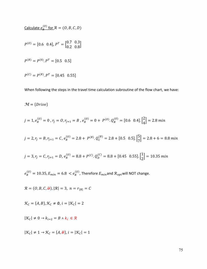
75
Calculate 𝑒𝑅(𝑂)
for ℛ = (𝑂, 𝐵, 𝐶, 𝐷)
𝑃(𝑂) = [0.6 0.4], 𝑃𝑇 = [0.7 0.30.2 0.8
]
𝑃(𝐵) = 𝑃(0). 𝑃𝑇 = [0.5 0.5]
𝑃(𝐶) = 𝑃(𝐵). 𝑃𝑇 = [0.45 0.55]
When following the steps in the travel time calculation subroutine of the flow chart, we have:
M = {𝐷𝑟𝑖𝑣𝑒}
𝑗 = 1, 𝑒𝑅(𝑂)
= 0 , 𝑟𝑗 = 𝑂, 𝑟𝑗+1 = 𝐵 , 𝑒𝑅(𝑂)
= 0 + 𝑃(𝑂). 𝑄𝐵(𝑂)
= [0.6 0.4]. [24
] = 2.8 𝑚𝑖𝑛
𝑗 = 2, 𝑟𝑗 = 𝐵, 𝑟𝑗+1 = 𝐶, 𝑒𝑅(𝑂)
= 2.8 + 𝑃(𝐵). 𝑄𝐶(𝐵)
= 2.8 + [0.5 0.5]. [57
] = 2.8 + 6 = 8.8 𝑚𝑖𝑛
𝑗 = 3, 𝑟𝑗 = 𝐶, 𝑟𝑗+1 = 𝐷, 𝑒𝑅(𝑂)
= 8.8 + 𝑃(𝐶). 𝑄𝐷(𝐶)
= 8.8 + [0.45 0.55]. [12
] = 10.35 𝑚𝑖𝑛
𝑒𝑅(𝑂)
= 10.35, 𝐸𝑚𝑖𝑛 = 6.8 < 𝑒𝑅(𝑂)
, Therefore 𝐸𝑚𝑖𝑛and ℛ𝑜𝑝𝑡will NOT change.
ℛ = (𝑂, 𝐵, 𝐶, 𝐷), |ℛ| = 3, 𝑛 = 𝑟|ℛ| = 𝐶
𝒦𝐶 = {𝐴, 𝐵}, 𝒦𝐶 ≠ ∅, 𝑖 = |𝒦𝐶| = 2
|𝒦𝐶| ≠ 0 → 𝑘𝑖=2 = 𝐵 ˄ 𝑘𝑖 ∈ ℛ
|𝒦𝐶| ≠ 1 → 𝒦𝐶 = {𝐴, 𝐵}, 𝑖 = |𝒦𝐶| = 1

76
|𝒦𝐶| ≠ 0 → 𝑘𝑖=1 = 𝐴 ˄ 𝑘𝑖 ∉ ℛ
𝑛 = 𝑘𝑖 = 𝐴 (𝑛 ≠ 𝐷), 𝒦𝐶 = {𝐴}, ℛ = (𝑂, 𝐵, 𝐶, 𝐴)
There is no node from 𝐴 to destination, which means this loop-processed node is a dead-end
node. The algorithm is able to identify this situation and it returns to the previous node by
following the steps below:
Identify adjacent nodes to 𝑛 = 𝐴: 𝒦𝐴 = {𝑂, 𝐵, 𝐶}, 𝑖 = |𝒦𝐴| = 3
|𝒦𝐴| ≠ 0 → 𝑘𝑖=3 = 𝐶 ˄ 𝑘𝑖 ∈ ℛ
|𝒦𝐴| ≠ 1 → 𝒦𝐴 = {𝑂, 𝐵, 𝐶}, 𝑖 = |𝒦𝐴| = 2
|𝒦𝐴| ≠ 0 → 𝑘𝑖=2 = 𝐵 ˄ 𝑘𝑖 ∈ ℛ
|𝒦𝐴| ≠ 1 → 𝒦𝐴 = {𝑂, 𝐵}, 𝑖 = |𝒦𝐴| = 1
|𝒦𝐴| ≠ 0 → 𝑘𝑖=1 = 𝑂 ˄ 𝑘𝑖 ∈ ℛ
|𝒦𝐴| = 1 → ℛ = (𝑂, 𝐵, 𝐶, 𝐴),ℛ ≠ ∅ → 𝑛 = 𝑟|ℛ| = 𝐶, 𝑖 = |𝒦𝐶| = 0
(𝑓𝑟𝑜𝑚 𝑎𝑏𝑜𝑣𝑒: 𝒦𝐶 = ∅)
𝐴 was a dead-end node and was successfully removed from the route list. Now the algorithm
processes the preceding node in the list, 𝐶.
|𝒦𝐶| = 0 → ℛ = (𝑂, 𝐵, 𝐶),ℛ ≠ ∅ → 𝑛 = 𝑟|ℛ| = 𝐵, 𝑖 = |𝒦𝐵| = 2

77
(𝑓𝑟𝑜𝑚 𝑎𝑏𝑜𝑣𝑒: 𝒦𝐵 = {𝑂, 𝐴})
Since there is no unvisited nodes available adjacent to node 𝐶, this is also be removed from the
route list and the node before that (𝐵) becomes the current node. By removing these nodes
and identifying them as visited, the algorithm avoids looping infinitely. The process of
identifying other routes continues from node 𝐵, where there is one more unvisited adjacent
node available(i.e. 𝐴).
|𝒦𝐵| ≠ 0 → 𝑘𝑖=2 = 𝐴 ˄ 𝑘𝑖 ∉ ℛ
𝑛 = 𝑘𝑖 = 𝐴 (𝑛 ≠ 𝐷), 𝒦𝐵 = {𝑂, 𝐴},ℛ = (𝑂, 𝐵, 𝐴)
Re-identify adjacent nodes to 𝑛 = 𝐴: 𝒦𝐴 = {𝑂, 𝐵, 𝐶}, 𝑖 = |𝒦𝐴| = 3
|𝒦𝐴| ≠ 0
𝑘𝑖=3 = 𝐶 ˄ 𝑘𝑖 ∉ ℛ
𝑛 = 𝑘𝑖 = 𝐶 (𝑛 ≠ 𝐷), 𝒦𝐴 = {𝑂, 𝐵, 𝐶}, ℛ = (𝑂, 𝐵, 𝐴, 𝐶)
Re-identify adjacent nodes to 𝑛 = 𝐶: 𝒦𝐶 = {𝐴, 𝐵, 𝐷}, 𝑖 = |𝒦𝐶| = 3
|𝒦𝐶| ≠ 0
𝑘𝑖=3 = 𝐷 ˄ 𝑘𝑖 ∉ ℛ
𝑛 = 𝑘𝑖 = 𝐷 (𝑛 = 𝐷), 𝒦𝐶 = {𝐴, 𝐵, 𝐷}, ℛ = (𝑂, 𝐵, 𝐴, 𝐶, 𝐷)

78
Calculate 𝑒𝑅(𝑂)
for ℛ = (𝑂, 𝐵, 𝐴, 𝐶, 𝐷)
𝑃(𝑂) = [0.6 0.4], 𝑃𝑇 = [0.7 0.30.2 0.8
]
𝑃(𝐵) = 𝑃(0). 𝑃𝑇 = [0.5 0.5]
𝑃(𝐴) = 𝑃(𝐵). 𝑃𝑇 = [0.45 0.55]
𝑃(𝐶) = 𝑃(𝐴). 𝑃𝑇 = [0.425 0.575]
Following the steps in the travel time calculation subroutine:
M = {𝐷𝑟𝑖𝑣𝑒}
𝑗 = 1, 𝑒𝑅(𝑂)
= 0 , 𝑟𝑗 = 𝑂, 𝑟𝑗+1 = 𝐵 , 𝑒𝑅(𝑂)
= 0 + 𝑃(𝑂). 𝑄𝐵(𝑂)
= [0.6 0.4]. [24
] = 2.8 𝑚𝑖𝑛
𝑗 = 2, 𝑟𝑗 = 𝐵, 𝑟𝑗+1 = 𝐴, 𝑒𝑅(𝑂)
= 2.8 + 𝑃(𝐵). 𝑄𝐴(𝐵)
= 2.8 + [0.5 0.5]. [23
] = 2.8 + 2.5 = 5.3 𝑚𝑖𝑛
𝑗 = 3, 𝑟𝑗 = 𝐴, 𝑟𝑗+1 = 𝐶, 𝑒𝑅(𝑂)
= 5.3 + 𝑃(𝐴). 𝑄𝐶(𝐴)
= 5.3 + [0.45 0.55]. [25
] = 8.95 𝑚𝑖𝑛
𝑗 = 4, 𝑟𝑗 = 𝐶, 𝑟𝑗+1 = 𝐷, 𝑒𝑅(𝑂)
= 8.95 + 𝑃(𝐶). 𝑄𝐷(𝐶)
= 8.95 + [0.425 0.575]. [12
] = 10.525 𝑚𝑖𝑛
𝑒𝑅(𝑂)
= 10.525, 𝐸𝑚𝑖𝑛 = 6.8 < 𝑒𝑅(𝑂)
, Therefore 𝐸𝑚𝑖𝑛and ℛ𝑜𝑝𝑡will NOT change.
ℛ = (𝑂, 𝐵, 𝐴, 𝐶, 𝐷), |ℛ| = 4, 𝑛 = 𝑟|ℛ| = 𝐶
𝒦𝐶 = {𝐴, 𝐵}, 𝒦𝐶 ≠ ∅, 𝑖 = |𝒦𝐶| = 2
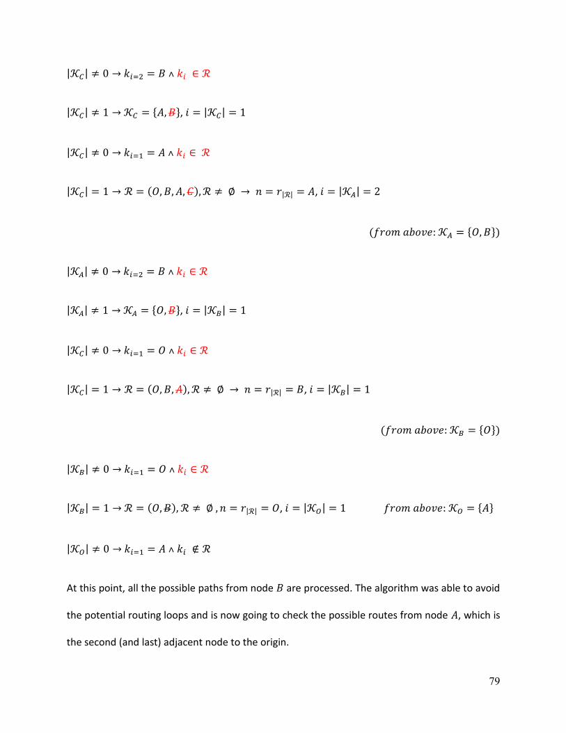
79
|𝒦𝐶| ≠ 0 → 𝑘𝑖=2 = 𝐵 ˄ 𝑘𝑖 ∈ ℛ
|𝒦𝐶| ≠ 1 → 𝒦𝐶 = {𝐴, 𝐵}, 𝑖 = |𝒦𝐶| = 1
|𝒦𝐶| ≠ 0 → 𝑘𝑖=1 = 𝐴 ˄ 𝑘𝑖 ∈ ℛ
|𝒦𝐶| = 1 → ℛ = (𝑂, 𝐵, 𝐴, 𝐶), ℛ ≠ ∅ → 𝑛 = 𝑟|ℛ| = 𝐴, 𝑖 = |𝒦𝐴| = 2
(𝑓𝑟𝑜𝑚 𝑎𝑏𝑜𝑣𝑒: 𝒦𝐴 = {𝑂, 𝐵})
|𝒦𝐴| ≠ 0 → 𝑘𝑖=2 = 𝐵 ˄ 𝑘𝑖 ∈ ℛ
|𝒦𝐴| ≠ 1 → 𝒦𝐴 = {𝑂, 𝐵}, 𝑖 = |𝒦𝐵| = 1
|𝒦𝐶| ≠ 0 → 𝑘𝑖=1 = 𝑂 ˄ 𝑘𝑖 ∈ ℛ
|𝒦𝐶| = 1 → ℛ = (𝑂, 𝐵, 𝐴), ℛ ≠ ∅ → 𝑛 = 𝑟|ℛ| = 𝐵, 𝑖 = |𝒦𝐵| = 1
(𝑓𝑟𝑜𝑚 𝑎𝑏𝑜𝑣𝑒: 𝒦𝐵 = {𝑂})
|𝒦𝐵| ≠ 0 → 𝑘𝑖=1 = 𝑂 ˄ 𝑘𝑖 ∈ ℛ
|𝒦𝐵| = 1 → ℛ = (𝑂, 𝐵), ℛ ≠ ∅ , 𝑛 = 𝑟|ℛ| = 𝑂, 𝑖 = |𝒦𝑂| = 1 𝑓𝑟𝑜𝑚 𝑎𝑏𝑜𝑣𝑒: 𝒦𝑂 = {𝐴}
|𝒦𝑂| ≠ 0 → 𝑘𝑖=1 = 𝐴 ˄ 𝑘𝑖 ∉ ℛ
At this point, all the possible paths from node 𝐵 are processed. The algorithm was able to avoid
the potential routing loops and is now going to check the possible routes from node 𝐴, which is
the second (and last) adjacent node to the origin.

80
𝑛 = 𝑘𝑖 = 𝐴 (𝑛 ≠ 𝐷), 𝒦𝑂 = {𝐴}, ℛ = (𝑂, 𝐴)
It should be noted that now 𝒦𝑂 = ∅, which means that there is no other node to process, after
identifying all possible paths from 𝐴 to destination.
Re-identify adjacent nodes to 𝑛 = 𝐴: 𝒦𝐴 = {𝑂, 𝐵, 𝐶}, 𝑖 = |𝒦𝐴| = 3
|𝒦𝐴| ≠ 0
𝑘𝑖=3 = 𝐶 ˄ 𝑘𝑖 ∉ ℛ
𝑛 = 𝑘𝑖 = 𝐶 (𝑛 ≠ 𝐷), 𝒦𝐴 = {𝑂, 𝐵, 𝐶}, ℛ = (𝑂, 𝐴, 𝐶)
Re-identify adjacent nodes to 𝑛 = 𝐶: 𝒦𝐶 = {𝐴, 𝐵, 𝐷}, 𝑖 = |𝒦𝐶| = 3
|𝒦𝐶| ≠ 0
𝑘𝑖=3 = 𝐷 ˄ 𝑘𝑖 ∉ ℛ
𝑛 = 𝑘𝑖 = 𝐷 (𝑛 = 𝐷), 𝒦𝐶 = {𝐴, 𝐵, 𝐷}, ℛ = (𝑂, 𝐴, 𝐶, 𝐷)
Calculate 𝑒𝑅(𝑂)
for ℛ = (𝑂, 𝐴, 𝐶, 𝐷)
𝑃(𝑂) = [0.6 0.4], 𝑃𝑇 = [0.7 0.30.2 0.8
]
𝑃(𝐴) = 𝑃(0). 𝑃𝑇 = [0.5 0.5]
𝑃(𝐶) = 𝑃(𝐴). 𝑃𝑇 = [0.45 0.55]

81
The travel time calculation is performed using the subroutine of the flow chart (Figure 3):
M = {𝐷𝑟𝑖𝑣𝑒}
𝑗 = 1, 𝑒𝑅(𝑂)
= 0 , 𝑟𝑗 = 𝑂, 𝑟𝑗+1 = 𝐴 , 𝑒𝑅(𝑂)
= 0 + 𝑃(𝑂). 𝑄𝐴(𝑂)
= [0.6 0.4]. [13
] = 1.8 𝑚𝑖𝑛
𝑗 = 2, 𝑟𝑗 = 𝐴, 𝑟𝑗+1 = 𝐶, 𝑒𝑅(𝑂)
= 1.8 + 𝑃(𝐴). 𝑄𝐶(𝐴)
= 1.8 + [0.5 0.5]. [25
] = 1.8 + 3.5 = 5.3 𝑚𝑖𝑛
𝑗 = 3, 𝑟𝑗 = 𝐶, 𝑟𝑗+1 = 𝐷, 𝑒𝑅(𝑂)
= 8.8 + 𝑃(𝐶). 𝑄𝐷(𝐶)
= 5.3 + [0.45 0.55]. [12
] = 6.85 𝑚𝑖𝑛
𝑒𝑅(𝑂)
= 6.85, 𝐸𝑚𝑖𝑛 = 6.8 < 𝑒𝑅(𝑂)
, Therefore 𝐸𝑚𝑖𝑛and ℛ𝑜𝑝𝑡will NOT change.
ℛ = (𝑂, 𝐴, 𝐶, 𝐷), |ℛ| = 3, 𝑛 = 𝑟|ℛ| = 𝐶
𝒦𝐶 = {𝐴, 𝐵}, 𝐾𝐶 ≠ ∅, 𝑖 = |𝒦𝐶| = 2
|𝒦𝐶| ≠ 0 → 𝑘𝑖=2 = 𝐵 ˄ 𝑘𝑖 ∉ ℛ
𝑛 = 𝑘𝑖 = 𝐵 (𝑛 ≠ 𝐷), 𝒦𝐶 = {𝐴, 𝐵}, ℛ = (𝑂, 𝐴, 𝐶, 𝐵)
Re-identify adjacent nodes to 𝑛 = 𝐵: 𝒦𝐵 = {𝑂, 𝐴, 𝐶, 𝐷, 𝑟1}, 𝑖 = |𝒦𝐵| = 5
𝒦𝐵 = {𝑂, 𝐴, 𝐶, 𝐷, 𝑟1}, Set the size of 𝒦𝐵: 𝑖 = 5
|𝒦𝐵| ≠ 0
𝑘𝑖=5 = 𝑟1 ˄ 𝑘𝑖 ∉ ℛ

82
𝑛 = 𝑘𝑖 = 𝑟1 (𝑛 ≠ 𝐷), 𝒦𝐵 = {𝑂, 𝐴, 𝐶, 𝐷, 𝑟1}, ℛ = (𝑂, 𝐴, 𝐶, 𝐵, 𝑟1)
Identify adjacent nodes to 𝑛 = 𝑟1: 𝒦𝑟1= {𝐵, 𝑟2}, 𝑖 = |𝒦𝑟1
| = 2
|𝒦𝑟1| ≠ 0
𝑘𝑖=2 = 𝑟2 ˄ 𝑘𝑖 ∉ ℛ
𝑛 = 𝑘𝑖 = 𝑟2 (𝑛 ≠ 𝐷), 𝒦𝑟1= {𝐵, 𝑟2}, ℛ = (𝑂, 𝐴, 𝐶, 𝐵, 𝑟1, 𝑟2)
Identify adjacent nodes to 𝑛 = 𝑟2: 𝒦𝑟2= {𝑟1, 𝐷}, 𝑖 = |𝒦𝑟2
| = 2
|𝒦𝑟2| ≠ 0
𝑘𝑖=2 = 𝐷 ˄ 𝑘𝑖 ∉ ℛ
𝑛 = 𝑘𝑖 = 𝐷 (𝑛 = 𝐷), 𝒦𝑟2= {𝐵, 𝐷}, ℛ = (𝑂, 𝐴, 𝐶, 𝐵, 𝑟1, 𝑟2, 𝐷)
Calculate 𝑒𝑅(𝑂)
for ℛ = (𝑂, 𝐴, 𝐶, 𝐵, 𝑟1, 𝑟2, 𝐷)
𝑃(𝑂) = [0.6 0.4], 𝑃𝑇 = [0.7 0.30.2 0.8
]
𝑃(𝐴) = 𝑃(0). 𝑃𝑇 = [0.5 0.5]
𝑃(𝐶) = 𝑃(𝐴). 𝑃𝑇 = [0.45 0.55]

83
There is no traffic conditions defined for Transit or Walk modes. The travel time calculation is
performed using the subroutine of the flow chart (Figure 3). First, the transportation modes
associated with each node in route ℛ is identified:
M = {𝐷𝑟𝑖𝑣𝑒, 𝐷𝑟𝑖𝑣𝑒, 𝐷𝑟𝑖𝑣𝑒, 𝑊𝑎𝑙𝑘, 𝑇𝑟𝑎𝑛𝑠𝑖𝑡, 𝑊𝑎𝑙𝑘}
Other initializations: 𝑗 = 1, 𝑚0 = 𝐷𝑟𝑖𝑣𝑒, 𝑡𝑟𝑎𝑛𝑓 = 0, 𝑤 = 0, 𝑒𝑅(𝑂)
= 0
𝑗 = 1, 𝑒𝑅(𝑂)
= 0 , 𝑟𝑗 = 𝑂,M𝑗 = 𝐷𝑟𝑖𝑣𝑒, 𝑟𝑗+1 = 𝐴 , 𝑒𝑅(𝑂)
= 0 + 𝑃(𝑂). 𝑄𝐴(𝑂)
= [0.6 0.4]. [13
] =
1.8 𝑚𝑖𝑛
𝑗 = 2, 𝑟𝑗 = 𝐴,M𝑗 = 𝐷𝑟𝑖𝑣𝑒, 𝑟𝑗+1 = 𝐶, 𝑒𝑅(𝑂)
= 1.8 + 𝑃(𝐴). 𝑄𝐶(𝐴)
= 1.8 + [0.5 0.5]. [25
] = 1.8 +
3.5 = 5.3 𝑚𝑖𝑛
𝑗 = 3, 𝑟𝑗 = 𝐶,M𝑗 = 𝐷𝑟𝑖𝑣𝑒, 𝑟𝑗+1 = 𝐵, 𝑒𝑅(𝑂)
= 5.3 + 𝑃(𝐶). 𝑄𝐵(𝐶)
= 5.3 + [0.45 0.55]. [57
] =
11.4 𝑚𝑖𝑛
𝑗 = 4, 𝑟𝑗 = 𝐵,M𝑗 = 𝑊𝑎𝑙𝑘, 𝑟𝑗+1 = 𝑟1,
M𝑗 ≠ 𝑚0: mode change happened from node 𝑗 to 𝑗 + 1. 𝑡𝑟𝑎𝑛𝑠𝑓 < 4
𝑡𝑟𝑎𝑛𝑓 = 1, 𝑤 = 𝑝𝑎𝑟𝑘 = 5 𝑚𝑖𝑛 (additional 5 minutes to park the car and get to the subway
entrance), 𝑚0 = M𝑗 = 𝑊𝑎𝑙𝑘
𝑒𝑅(𝑂)
= 11.4 + 𝑤 + 𝑄𝑟1
(𝐵)= 11.4 + 5 + 1 = 17.4 min

84
𝑗 = 5, 𝑤 = 0, 𝑟𝑗 = 𝑟1,M𝑗 = 𝑇𝑟𝑎𝑛𝑠𝑖𝑡, 𝑟𝑗+1 = 𝑟2
M𝑗 ≠ 𝑚0: mode change happened from node 𝑗 to 𝑗 + 1. 𝑡𝑟𝑎𝑛𝑠𝑓 < 4
Assuming traveler started at 4:00 pm and the subway runs at 5 minute intervals between 4 and
5 pm:
𝑡𝑟𝑎𝑛𝑓 = 2, 𝑤 = 𝑤𝑎𝑖𝑡𝑖𝑛𝑔 𝑡𝑖𝑚𝑒 = 04: 20: 00 − (04: 00: 00 + 0: 17: 24) = 2.6 𝑚𝑖𝑛
𝑚0 = M𝑗 = 𝑇𝑟𝑎𝑛𝑠𝑖𝑡
𝑒𝑅(𝑂)
= 17.4 + 2.6 + 𝑄𝑟2
(𝑟1)= 17.4 + 2.6 + 2 = 22 𝑚𝑖𝑛
𝑗 = 6, 𝑤 = 0, 𝑟𝑗 = 𝑟2,M𝑗 = 𝑊𝑎𝑙𝑘, 𝑟𝑗+1 = 𝐷
M𝑗 ≠ 𝑚0: mode change happened from node 𝑗 to 𝑗 + 1. 𝑡𝑟𝑎𝑛𝑠𝑓 < 4
𝑡𝑟𝑎𝑛𝑠𝑓 = 2,
𝑒𝑅(𝑂)
= 22 + 0 + 𝑄𝐷(𝑟2)
= 22 + 1 = 23 𝑚𝑖𝑛
𝑒𝑅(𝑂)
= 23, 𝐸𝑚𝑖𝑛 = 6.8 < 𝑒𝑅(𝑂)
, Therefore 𝐸𝑚𝑖𝑛and ℛ𝑜𝑝𝑡will NOT change.
ℛ = (𝑂, 𝐴, 𝐶, 𝐵, 𝑟1, 𝑟2, 𝐷), |ℛ| = 6, 𝑛 = 𝑟|ℛ| = 𝑟2
𝒦𝑟2= {𝐵}, 𝒦𝑟2
≠ ∅ → 𝑖 = | 𝒦𝑟2| = 1
| 𝒦𝑟2| ≠ 0 → 𝑘𝑖=1 = 𝐵 ˄ 𝑘𝑖 ∈ ℛ

85
| 𝒦𝑟2| = 1 → ℛ = (𝑂, 𝐴, 𝐶, 𝐵, 𝑟1, 𝑟2),ℛ ≠ ∅ → 𝑛 = 𝑟|ℛ| = 𝑟1, 𝑖 = |𝒦𝑟1
| = 0
| 𝒦𝑟1| ≠ 0 → 𝑘𝑖=1 = 𝐵 ˄ 𝑘𝑖 ∈ ℛ
| 𝒦𝑟1| = 1 → ℛ = (𝑂, 𝐴, 𝐶, 𝐵, 𝑟1),ℛ ≠ ∅ → 𝑛 = 𝑟|ℛ| = 𝐵, 𝑖 = |𝒦𝐵| = 4
(𝑓𝑟𝑜𝑚 𝑎𝑏𝑜𝑣𝑒 𝒦𝐵 = {𝑂, 𝐴, 𝐶, 𝐷})
𝑘𝑖=4 = 𝐷 ˄ 𝑘𝑖 ∉ ℛ
𝑛 = 𝑘𝑖 = 𝐷 (𝑛 = 𝐷), 𝒦𝐵 = {𝑂, 𝐴, 𝐶, 𝐷},ℛ = (𝑂, 𝐴, 𝐶, 𝐵, 𝐷)
Calculate 𝑒𝑅(𝑂)
for ℛ = (𝑂, 𝐴, 𝐶, 𝐵, 𝐷)
𝑃(𝑂) = [0.6 0.4], 𝑃𝑇 = [0.7 0.30.2 0.8
]
𝑃(𝐴) = 𝑃(0). 𝑃𝑇 = [0.5 0.5]
𝑃(𝐶) = 𝑃(𝐴). 𝑃𝑇 = [0.45 0.55]
𝑃(𝐵) = 𝑃(𝐶). 𝑃𝑇 = [0.425 0.575]
The travel time calculation is performed using the subroutine of the flow chart (Figure 3):
𝑗 = 1, 𝑒𝑅(𝑂)
= 0 , 𝑟𝑗 = 𝑂, 𝑟𝑗+1 = 𝐴 , 𝑒𝑅(𝑂)
= 0 + 𝑃(𝑂). 𝑄𝐴(𝑂)
= [0.6 0.4]. [13
] = 1.8 𝑚𝑖𝑛
𝑗 = 2, 𝑟𝑗 = 𝐴, 𝑟𝑗+1 = 𝐶, 𝑒𝑅(𝑂)
= 1.8 + 𝑃(𝐴). 𝑄𝐶(𝐴)
= 1.8 + [0.5 0.5]. [25
] = 1.8 + 3.5 = 5.3 𝑚𝑖𝑛

86
𝑗 = 3, 𝑟𝑗 = 𝐶, 𝑟𝑗+1 = 𝐵, 𝑒𝑅(𝑂)
= 5.3 + 𝑃(𝐶). 𝑄𝐵(𝐶)
= 5.3 + [0.45 0.55]. [57
] = 11.4 𝑚𝑖𝑛
𝑗 = 4, 𝑟𝑗 = 𝐵, 𝑟𝑗+1 = 𝐷, 𝑒𝑅(𝑂)
= 11.4 + 𝑃(𝐵). 𝑄𝐷(𝐵)
= 11.4 + [0.425 0.575]. [35
] = 15.5 𝑚𝑖𝑛
𝑒𝑅(𝑂)
= 15.5, 𝐸𝑚𝑖𝑛 = 6.8 < 𝑒𝑅(𝑂)
, Therefore 𝐸𝑚𝑖𝑛and ℛ𝑜𝑝𝑡will NOT change.
ℛ = (𝑂, 𝐴, 𝐶, 𝐵, 𝐷), |ℛ| = 4, 𝑛 = 𝑟|ℛ| = 𝐵
𝒦𝐵 = {𝑂, 𝐴, 𝐶}, 𝒦𝐵 ≠ ∅, 𝑖 = |𝒦𝐵| = 3
|𝒦𝐵| ≠ 0 → 𝑘𝑖=3 = 𝐶 ˄ 𝑘𝑖 ∈ ℛ
|𝒦𝐵| ≠ 1 → 𝒦𝐵 = {𝑂, 𝐴, 𝐶}, 𝑖 = |𝒦𝐵| = 2
|𝒦𝐵| ≠ 0 → 𝑘𝑖=2 = 𝐴 ˄ 𝑘𝑖 ∈ ℛ
|𝒦𝐵| ≠ 1 → 𝒦𝐵 = {𝑂, 𝐴}, 𝑖 = |𝒦𝐵| = 1
|𝒦𝐵| ≠ 0 → 𝑘𝑖=1 = 𝑂 ˄ 𝑘𝑖 ∈ ℛ
|𝒦𝐵| = 1 → ℛ = (𝑂, 𝐴, 𝐶, 𝐵), ℛ ≠ ∅ → 𝑛 = 𝑟|ℛ| = 𝐶, 𝑖 = |𝒦𝐶| = 1
(𝑓𝑟𝑜𝑚 𝑎𝑏𝑜𝑣𝑒: 𝒦𝐶 = {𝐴})
|𝒦𝐶| ≠ 0 → 𝑘𝑖=1 = 𝐴 ˄ 𝑘𝑖 ∈ ℛ
|𝒦𝐶| = 1 → ℛ = (𝑂, 𝐴, 𝐶), ℛ ≠ ∅ → 𝑛 = 𝑟|ℛ| = 𝐴, 𝑖 = |𝒦𝐴| = 2
(𝑓𝑟𝑜𝑚 𝑎𝑏𝑜𝑣𝑒 𝒦𝐴 = {𝑂, 𝐵})
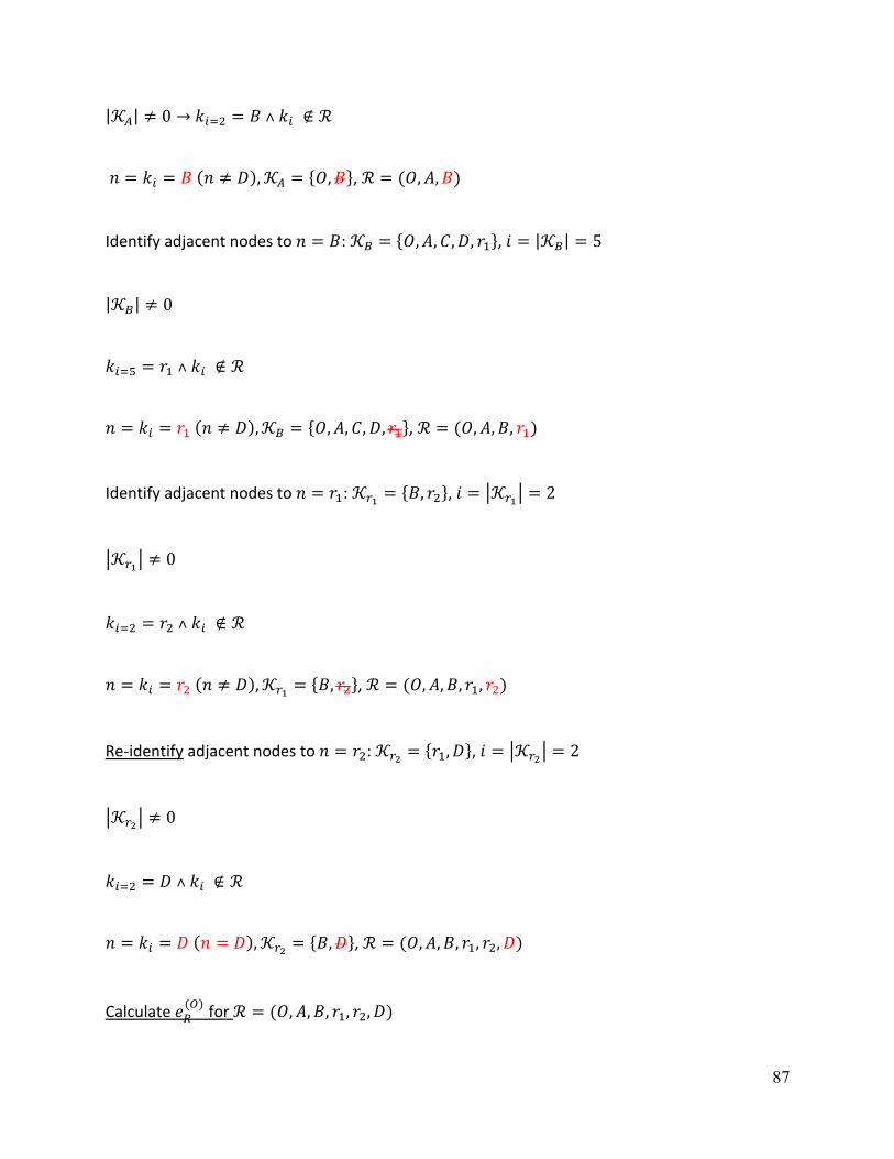
87
|𝒦𝐴| ≠ 0 → 𝑘𝑖=2 = 𝐵 ˄ 𝑘𝑖 ∉ ℛ
𝑛 = 𝑘𝑖 = 𝐵 (𝑛 ≠ 𝐷), 𝒦𝐴 = {𝑂, 𝐵}, ℛ = (𝑂, 𝐴, 𝐵)
Identify adjacent nodes to 𝑛 = 𝐵: 𝒦𝐵 = {𝑂, 𝐴, 𝐶, 𝐷, 𝑟1}, 𝑖 = |𝒦𝐵| = 5
|𝒦𝐵| ≠ 0
𝑘𝑖=5 = 𝑟1 ˄ 𝑘𝑖 ∉ ℛ
𝑛 = 𝑘𝑖 = 𝑟1 (𝑛 ≠ 𝐷), 𝒦𝐵 = {𝑂, 𝐴, 𝐶, 𝐷, 𝑟1}, ℛ = (𝑂, 𝐴, 𝐵, 𝑟1)
Identify adjacent nodes to 𝑛 = 𝑟1: 𝒦𝑟1= {𝐵, 𝑟2}, 𝑖 = |𝒦𝑟1
| = 2
|𝒦𝑟1| ≠ 0
𝑘𝑖=2 = 𝑟2 ˄ 𝑘𝑖 ∉ ℛ
𝑛 = 𝑘𝑖 = 𝑟2 (𝑛 ≠ 𝐷), 𝒦𝑟1= {𝐵, 𝑟2}, ℛ = (𝑂, 𝐴, 𝐵, 𝑟1, 𝑟2)
Re-identify adjacent nodes to 𝑛 = 𝑟2: 𝒦𝑟2= {𝑟1, 𝐷}, 𝑖 = |𝒦𝑟2
| = 2
|𝒦𝑟2| ≠ 0
𝑘𝑖=2 = 𝐷 ˄ 𝑘𝑖 ∉ ℛ
𝑛 = 𝑘𝑖 = 𝐷 (𝑛 = 𝐷), 𝒦𝑟2= {𝐵, 𝐷}, ℛ = (𝑂, 𝐴, 𝐵, 𝑟1, 𝑟2, 𝐷)
Calculate 𝑒𝑅(𝑂)
for ℛ = (𝑂, 𝐴, 𝐵, 𝑟1, 𝑟2, 𝐷)

88
𝑃(𝑂) = [0.6 0.4], 𝑃𝑇 = [0.7 0.30.2 0.8
]
𝑃(𝐴) = 𝑃(0). 𝑃𝑇 = [0.5 0.5]
There is no traffic conditions defined for Transit or Walk modes. The travel time calculation is
performed using the subroutine of the flow chart (Figure 3). First, the transportation modes
associated with each node in route ℛ is identified:
M = {𝐷𝑟𝑖𝑣𝑒, 𝐷𝑟𝑖𝑣𝑒, 𝑊𝑎𝑙𝑘, 𝑇𝑟𝑎𝑛𝑠𝑖𝑡, 𝑊𝑎𝑙𝑘}
Other initializations: 𝑗 = 1, 𝑚0 = 𝐷𝑟𝑖𝑣𝑒, 𝑡𝑟𝑎𝑛𝑠𝑓 = 0, 𝑤 = 0, 𝑒𝑅(𝑂)
= 0
𝑗 = 1, 𝑒𝑅(𝑂)
= 0 , 𝑟𝑗 = 𝑂, 𝑟𝑗+1 = 𝐴 , 𝑒𝑅(𝑂)
= 0 + 𝑃(𝑂). 𝑄𝐴(𝑂)
= [0.6 0.4]. [13
] = 1.8 𝑚𝑖𝑛
𝑗 = 2, 𝑟𝑗 = 𝐴, 𝑟𝑗+1 = 𝐵, 𝑒𝑅(𝑂)
= 1.8 + 𝑃(𝐴). 𝑄𝐵(𝐴)
= 1.8 + [0.5 0.5]. [23
] = 1.8 + 2.5 = 4.3 𝑚𝑖𝑛
𝑗 = 3, 𝑟𝑗 = 𝐵,M𝑗 = 𝑊𝑎𝑙𝑘, 𝑟𝑗+1 = 𝑟1,
M𝑗 ≠ 𝑚0: mode change happened from node 𝑗 to 𝑗 + 1. 𝑡𝑟𝑎𝑛𝑠𝑓 < 4
𝑡𝑟𝑎𝑛𝑓 = 1, 𝑤 = 𝑝𝑎𝑟𝑘 = 5 𝑚𝑖𝑛 (additional 5 minutes to park the car and get to the subway
entrance), 𝑚0 = M𝑗 = 𝑊𝑎𝑙𝑘
𝑒𝑅(𝑂)
= 4.3 + 𝑤 + 𝑄𝑟1
(𝐵)= 4.3 + 5 + 1 = 10.3 min
𝑗 = 4, 𝑤 = 0, 𝑟𝑗 = 𝑟1,M𝑗 = 𝑇𝑟𝑎𝑛𝑠𝑖𝑡, 𝑟𝑗+1 = 𝑟2

89
M𝑗 ≠ 𝑚0: mode change happened from node 𝑗 to 𝑗 + 1. 𝑡𝑟𝑎𝑛𝑠𝑓 < 4
Assuming traveler started at 4:00 pm and the subway runs at 5 minute intervals between 4 and
5 pm:
𝑡𝑟𝑎𝑛𝑓 = 2, 𝑤 = 𝑤𝑎𝑖𝑡𝑖𝑛𝑔 𝑡𝑖𝑚𝑒 = 04: 15: 00 − (04: 00: 00 + 00: 10: 18) = 4.7 𝑚𝑖𝑛
𝑚0 = M𝑗 = 𝑇𝑟𝑎𝑛𝑠𝑖𝑡
𝑒𝑅(𝑂)
= 10.3 + 4.7 + 𝑄𝑟2
(𝑟1)= 10.3 + 4.7 + 2 = 17 𝑚𝑖𝑛
𝑗 = 5, 𝑤 = 0, 𝑟𝑗 = 𝑟2,M𝑗 = 𝑊𝑎𝑙𝑘, 𝑟𝑗+1 = 𝐷
M𝑗 ≠ 𝑚0: mode change happened from node 𝑗 to 𝑗 + 1. 𝑡𝑟𝑎𝑛𝑠𝑓 < 4
𝑡𝑟𝑎𝑛𝑠𝑓 = 2,
𝑒𝑅(𝑂)
= 17 + 0 + 𝑄𝐷(𝑟2)
= 17 + 1 = 18 𝑚𝑖𝑛
𝑒𝑅(𝑂)
= 18, 𝐸𝑚𝑖𝑛 = 6.8 < 𝑒𝑅(𝑂)
, Therefore 𝐸𝑚𝑖𝑛and ℛ𝑜𝑝𝑡will NOT change.
ℛ = (𝑂, 𝐴, 𝐵, 𝑟1, 𝑟2, 𝐷), |ℛ| = 5, 𝑛 = 𝑟|ℛ| = 𝑟2
𝒦𝑟2= {𝐵}, 𝒦𝑟2
≠ ∅ → 𝑖 = |𝒦𝑟2| = 1
| 𝒦𝑟2| ≠ 0 → 𝑘𝑖=1 = 𝐵 ˄ 𝑘𝑖 ∈ ℛ
|𝒦𝑟2| = 1 → ℛ = (𝑂, 𝐴, 𝐵, 𝑟1, 𝑟2),ℛ ≠ ∅ → 𝑛 = 𝑟|ℛ| = 𝑟1, 𝑖 = |𝒦𝑟1
| = 0

90
|𝒦𝑟1| ≠ 0 → 𝑘𝑖=1 = 𝐵 ˄ 𝑘𝑖 ∈ ℛ
| 𝒦𝑟1| = 1 → ℛ = (𝑂, 𝐴, 𝐵, 𝑟1),ℛ ≠ ∅ → 𝑛 = 𝑟|ℛ| = 𝐵, 𝑖 = |𝒦𝐵| = 4
(𝑓𝑟𝑜𝑚 𝑎𝑏𝑜𝑣𝑒 𝒦𝐵 = {𝑂, 𝐴, 𝐶, 𝐷})
𝑘𝑖=4 = 𝐷 ˄ 𝑘𝑖 ∉ ℛ
𝑛 = 𝑘𝑖 = 𝐷 (𝑛 = 𝐷), 𝒦𝐵 = {𝑂, 𝐴, 𝐶, 𝐷},ℛ = (𝑂, 𝐴, 𝐵, 𝐷)
Calculate 𝑒𝑅(𝑂)
for ℛ = (𝑂, 𝐴, 𝐵, 𝐷)
𝑃(𝑂) = [0.6 0.4], 𝑃𝑇 = [0.7 0.30.2 0.8
]
𝑃(𝐴) = 𝑃(0). 𝑃𝑇 = [0.5 0.5]
𝑃(𝐵) = 𝑃(𝐴). 𝑃𝑇 = [0.45 0.55]
The travel time calculation is performed using the subroutine of the flow chart (Figure 3):
M = {𝐷𝑟𝑖𝑣𝑒}
𝑗 = 1, 𝑒𝑅(𝑂)
= 0 , 𝑟𝑗 = 𝑂, 𝑟𝑗+1 = 𝐴 , 𝑒𝑅(𝑂)
= 0 + 𝑃(𝑂). 𝑄𝐴(𝑂)
= [0.6 0.4]. [13
] = 1.8 𝑚𝑖𝑛
𝑗 = 2, 𝑟𝑗 = 𝐴, 𝑟𝑗+1 = 𝐵, 𝑒𝑅(𝑂)
= 1.8 + 𝑃(𝐴). 𝑄𝐵(𝐴)
= 1.8 + [0.5 0.5]. [23
] = 1.8 + 2.5 = 4.3 𝑚𝑖𝑛
𝑗 = 3, 𝑟𝑗 = 𝐵, 𝑟𝑗+1 = 𝐷, 𝑒𝑅(𝑂)
= 4.3 + 𝑃(𝐵). 𝑄𝐷(𝐵)
= 4.3 + [0.45 0.55]. [35
] = 8.4 𝑚𝑖𝑛

91
𝑒𝑅(𝑂)
= 8.4, 𝐸𝑚𝑖𝑛 = 6.8 < 𝑒𝑅(𝑂)
, Therefore 𝐸𝑚𝑖𝑛and ℛ𝑜𝑝𝑡will NOT change.
ℛ = (𝑂, 𝐴, 𝐵, 𝐷), |ℛ| = 3, 𝑛 = 𝑟|ℛ| = 𝐵
𝒦𝐵 = {𝑂, 𝐴, 𝐶}, 𝒦𝐵 ≠ ∅, 𝑖 = |𝒦𝐵| = 3
|𝒦𝐵| ≠ 0 → 𝑘𝑖=3 = 𝐶 ˄ 𝑘𝑖 ∉ ℛ
𝑛 = 𝑘𝑖 = 𝐶 (𝑛 ≠ 𝐷), 𝒦𝐵 = {𝑂, 𝐴, 𝐶}, ℛ = (𝑂, 𝐴, 𝐵, 𝐶)
Identify adjacent nodes to 𝑛 = 𝐶: 𝒦𝐶 = {𝐴, 𝐵, 𝐷}, 𝑖 = |𝒦𝐶| = 3
|𝒦𝐶| ≠ 0
𝑘𝑖=3 = 𝐷 ˄ 𝑘𝑖 ∉ ℛ
𝑛 = 𝑘𝑖 = 𝐷 (𝑛 = 𝐷), 𝒦𝐶 = {𝐴, 𝐵, 𝐷}, ℛ = (𝑂, 𝐴, 𝐵, 𝐶, 𝐷)
Calculate 𝑒𝑅(𝑂)
for ℛ = (𝑂, 𝐴, 𝐵, 𝐶, 𝐷)
𝑃(𝑂) = [0.6 0.4], 𝑃𝑇 = [0.7 0.30.2 0.8
]
𝑃(𝐴) = 𝑃(0). 𝑃𝑇 = [0.5 0.5]
𝑃(𝐵) = 𝑃(𝐴). 𝑃𝑇 = [0.45 0.55]
𝑃(𝐶) = 𝑃(𝐵). 𝑃𝑇 = [0.425 0.575]
The travel time calculation is performed using the subroutine of the flow chart (Figure 3):

92
M = {𝐷𝑟𝑖𝑣𝑒}
𝑗 = 1, 𝑒𝑅(𝑂)
= 0 , 𝑟𝑗 = 𝑂, 𝑟𝑗+1 = 𝐴 , 𝑒𝑅(𝑂)
= 0 + 𝑃(𝑂). 𝑄𝐴(𝑂)
= [0.6 0.4]. [13
] = 1.8 𝑚𝑖𝑛
𝑗 = 2, 𝑟𝑗 = 𝐴, 𝑟𝑗+1 = 𝐵, 𝑒𝑅(𝑂)
= 1.8 + 𝑃(𝐴). 𝑄𝐵(𝐴)
= 1.8 + [0.5 0.5]. [23
] = 1.8 + 2.5 = 4.3 𝑚𝑖𝑛
𝑗 = 3, 𝑟𝑗 = 𝐵, 𝑟𝑗+1 = 𝐶, 𝑒𝑅(𝑂)
= 4.3 + 𝑃(𝐵). 𝑄𝐶(𝐵)
= 4.3 + [0.45 0.55]. [57
] = 10.4 𝑚𝑖𝑛
𝑗 = 4, 𝑟𝑗 = 𝐶, 𝑟𝑗+1 = 𝐷, 𝑒𝑅(𝑂)
= 10.4 + 𝑃(𝐶). 𝑄𝐷(𝐶)
= 10.4 + [0.425 0.575]. [12
] = 11.97 𝑚𝑖𝑛
𝑒𝑅(𝑂)
= 11.97, 𝐸𝑚𝑖𝑛 = 6.8 < 𝑒𝑅(𝑂)
, Therefore 𝐸𝑚𝑖𝑛and ℛ𝑜𝑝𝑡will NOT change.
ℛ = (𝑂, 𝐴, 𝐵, 𝐶, 𝐷), |ℛ| = 4, 𝑛 = 𝑟|ℛ| = 𝐶
𝒦𝐶 = {𝐴, 𝐵}, 𝒦𝐵 ≠ ∅, 𝑖 = |𝒦𝐵| = 2
|𝒦𝐶| ≠ 0 → 𝑘𝑖=2 = 𝐵 ˄ 𝑘𝑖 ∈ ℛ
|𝒦𝐶| ≠ 1 → 𝒦𝐶 = {𝐴, 𝐵}, 𝑖 = |𝒦𝐵| = 1
|𝒦𝐶| ≠ 0 → 𝑘𝑖=1 = 𝐴 ˄ 𝑘𝑖 ∈ ℛ
|𝒦𝐶| = 1 → ℛ = (𝑂, 𝐴, 𝐵, 𝐶), ℛ ≠ ∅ → 𝑛 = 𝑟|ℛ| = 𝐵, 𝑖 = |𝒦𝐵| = 2
(𝑓𝑟𝑜𝑚 𝑎𝑏𝑜𝑣𝑒: 𝒦𝐵 = {𝑂, 𝐴})
|𝒦𝐵| ≠ 0 → 𝑘𝑖=2 = 𝐴 ˄ 𝑘𝑖 ∈ ℛ

93
|𝒦𝐵| ≠ 1 → 𝒦𝐵 = {𝑂, 𝐴}, 𝑖 = |𝒦𝐵| = 1
|𝒦𝐵| ≠ 0 → 𝑘𝑖=1 = 𝑂 ˄ 𝑘𝑖 ∈ ℛ
|𝒦𝐵| = 1 → ℛ = (𝑂, 𝐴, 𝐵), ℛ ≠ ∅ → 𝑛 = 𝑟|ℛ| = 𝐴, 𝑖 = |𝒦𝐴| = 1
(𝑓𝑟𝑜𝑚 𝑎𝑏𝑜𝑣𝑒: 𝒦𝐴 = {𝑂})
|𝒦𝐴| ≠ 0 → 𝑘𝑖=1 = 𝑂 ˄ 𝑘𝑖 ∈ ℛ
|𝒦𝐴| = 1 → ℛ = (𝑂, 𝐴), ℛ ≠ ∅ → 𝑛 = 𝑟|ℛ| = 𝑂, 𝑖 = |𝒦𝑂| = 0
(𝑓𝑟𝑜𝑚 𝑎𝑏𝑜𝑣𝑒: 𝒦𝑂 = ∅)
𝒦𝑂 = ∅: which means that all adjacent nodes to the origin node have been visited.
|𝒦𝑂| = 0 → ℛ = (𝑂), ℛ = ∅ → Found the minimum path, Report:
𝐸𝑚𝑖𝑛 = 6.8 𝑚𝑖𝑛 , ℛ𝑜𝑝𝑡 = (𝑂, 𝐵, 𝐷)
3.5 Discussion on Transition Probability in Transportation Network
When the proposed algorithm is applied for route optimization in transportation networks, the
states of the system represent traffic conditions in the network. Similarly, transition probability
matrix denotes the probability of changes in traffic condition when travelling from one node to
another. In the previous sections, it was assumed that a unique transition probability matrix is
applicable at any location in the network. However, transportation network consists of
different road types (i.e. highway, arterial, etc.) which do not have the same traffic

94
characteristics (e.g. average speed, traffic volume). Consequently, there will be different
patterns of change in traffic conditions along each of these road types. Furthermore, traffic
conditions depend on the peak period and are not necessarily the same at different locations
within a large transportation network. Therefore, a more realistic representation of the
network should consider distinct transition probability matrices associated with different road
types and different peak directions within the network.
Using this approach, the estimation of transition probability matrix (𝑃𝑇) used to calculate the
state probability vector for the (𝑛 + 1)𝑡ℎ node, 𝑃(𝑛+1) = 𝑃(𝑛)𝑃𝑇 as shown in Figure 2, will be
specific to the link (road type) between nodes 𝑛 and 𝑛 + 1. According to Figure 2 there are
three different routes available between nodes 𝑛 and 𝑛 + 1, 𝑑1(𝑛)
, 𝑑2(𝑛)
𝑎𝑛𝑑 𝑑3(𝑛)
. Depending on
the type of the links related to each route, different transition probability matrices can be
defined and applied to each type.
The methodology described in the previous sections, applies the one-step transition probability
(𝑃𝑇) during each step when moving from one node to its adjacent node. For example, according
to Figure 2, when the traveler moves from node 𝑛 at time step 𝑡𝑛 to adjacent node (𝑛 + 1), the
time step at node 𝑛 + 1 is denoted by 𝑡𝑛+1. Expected penalty (travel time) from node 𝑛 to 𝑛 +
1 is the difference between 𝑡𝑛 and 𝑡𝑛+1, and is calculated using equation (3): 𝑒(𝑛) =
𝑃(𝑛). 𝑄𝑛+1(𝑛)
. Then the state probability vector for node 𝑛 + 1 is updated using equation (2) and
the one-step transition probability matrix: 𝑃(𝑛+1) = 𝑃(𝑛)𝑃𝑇 . Therefore, the probability vector
for each node is updated each time traveler moves to that node, without considering the
(𝑡𝑛+1 − 𝑡𝑛) time step and estimated travel time between the two nodes (𝑒(𝑛)).

95
As proposed previously in Section 3.3 collected traffic speed data is used to estimate the
transition probability matrix for the network. The resolution of the collected data (i.e. sampling
frequency) and the intervals for which speed data is aggregated represents the minimum time
period during which the changes in traffic conditions can be captured. For example, if
aggregated speed data for 2-minute intervals were used for estimating the transition
probability matrix, it can be assumed that if the travel time from one node to its adjacent node
is less than 2 minutes, the probability vector of traffic conditions at the adjacent node does not
need to be updated. Therefore, the resolution of traffic data can be used as an update
threshold for applying the transition probability matrix and updating state probabilities at each
node. Figure 5 presents a revised subroutine that can be used in the main flowchart to include
the time step threshold in probability matrix calculation for each node. The new procedure
temporarily stores the estimated travel time from node 𝑗 to node 𝑗 + 1 into 𝑡𝑗,𝑗+1, and checks it
against the defined threshold (𝑇𝑡𝑠). If the estimated time between the two nodes is equal or
greater than threshold, the traffic condition probability vector at node 𝑗 + 1 will be calculated
by applying the one-step transition probability matrix, as described in the previous sections.
However, if the expected travel time is less than the update threshold value, the state
probability vector at 𝑗 + 1 will not change, as compared to node 𝑗.
This enhancement of the proposed methodology can capture more accurately the stochastic
effects of traffic conditions along the network on travel time. The hypothetical example
network used previously in this section is also use here to demonstrate its benefits. However,
due to limitation of the available real-world data this enhancement has not been applied to any
of the case studies in this thesis.

96
Figure 5: Time-Step Threshold Optimization Subroutine
Calculate eR
(O) (expected travel time from O to D) Multi-modal Subroutinewith Time Step Threshold
No
Define MSet j=1
Set m0=Mj
Set transf=0
Set w=0
Set park=5
j < |R |
Calculate expected TT from O to rj+1
j=j+1
w=0
Yes
eR
(O)<Emin
No Emin=eR
(O)
Ropt=R
R=R\{r|R|}
n = r|R|
Kn== Ø |R |==1
No
Yes
Found Emin and
Ropt
Yes
Yes
No
Definitions
: Vector of the probabilities of the system to
be in each state (traffic conditions)
: Vector of travel time between rj and rj+1 in
each possible state
: Set of transportation Modes related to each
node in route R: Threshold for minimum time to apply transition probability : Current transportation mode
: Number of mode transfers
: Waiting time for mode transfer: Time required to park the car
)()()()(
1. j
j
j r
r
rOO QPwee
RR
)( jrP
)(
1
j
j
r
rQ
0)( OeR
M
Mj is Transit?
Mj ≠ m0
transf=transf+1
transf > 2 OR
Mj is Drive
No
YesYes
No
No
Yes
0m
transf
w
m0 is Drive?w=park
m0 = Mj
No
Yes
park
Calculate w
m0 = Mj
Route identifiedCalculate eR (O)
tsT
tsT
Identify next Route
)()(
1, 1. j
j
j r
r
r
jj QPwt
tsjj Tt 1,
TrrPPP jj .
)()( 1
)()( 1 jj rrPP
Yes
No

97
The example provided in Section 3.4 applied the flowchart presented in Figure 3 to calculate
the optimal path between point O (origin) and point D (destination) in a sample network (Figure
4). To demonstrate the application of the proposed time-step threshold, the revised subroutine
shown in Figure 5 is used in conjunction with the flowchart. An arbitrary time-step threshold:
𝑇𝑡𝑟 = 5 𝑚𝑖𝑛𝑢𝑡𝑒𝑠 is assumed.
The optimal route calculation steps followed in the example to identify possible routes remain
the same and are not repeated here. The only difference between the new time-step threshold
subroutine and the one include in the flowchart is related to the calculation of 𝑒𝑅(𝑂)
. Therefore
the effect of introducing the time-step threshold in the example is shown by revising the 𝑒𝑅(𝑂)
calculations for each route identified in the previous example. Since the transition probability in
this example was only applied to “𝐷𝑟𝑖𝑣𝑖𝑛𝑔” mode, the changes are applied to the calculations
related to this mode. These changes and the revised calculation for the optimal path
calculations are listed in the following steps:
Calculate 𝑒𝑅(𝑂)
for ℛ = (𝑂, 𝐵, 𝑟1, 𝑟2, 𝐷)
Mode change occurs at node B and continues until destination.
Calculate 𝑒𝑅(𝑂)
for ℛ = (𝑂, 𝐵, 𝐷)
𝑃(𝑂) = [0.6 0.4], 𝑃𝑇 = [0.7 0.30.2 0.8
]
To re-calculate the optimal route by applying the time-step threshold subroutine, the travel
time between each pair of nodes is compared with 𝑇𝑡𝑟 = 5:

98
𝑗 = 1, 𝑒𝑅(𝑂)
= 0 + 𝑤 + 𝑃(𝑂). 𝑄𝐵(𝑂)
= 2.8 𝑚𝑖𝑛, 𝑡𝑗,𝑗+1 = 𝑃(𝑂). 𝑄𝐵(𝑂)
= 2.8 𝑚𝑖𝑛
𝑗 = 2, 𝑡𝑗,𝑗+1 < 𝑇𝑡𝑟 → 𝑃(𝐵) = 𝑃(𝑂) = [0.6 0.4]
Since the expected travel time from 𝑂 to 𝐵 is less than threshold, the transition probability
matrix is not considered for calculating the probability vector at node 𝐵.
𝑗 = 2, 𝑒𝑅(𝑂)
= 2.8 + 𝑃(𝐵). 𝑄𝐷(𝐵)
= 2.8 + [0.6 0.4]. [35
] = 2.8 + 3.8 = 6.6 𝑚𝑖𝑛
𝐸𝑚𝑖𝑛 = 𝑒𝑅(𝑂)
= 6.6 and ℛ𝑜𝑝𝑡 = ℛ = (𝑂, 𝐵, 𝐷)
The expected travel time calculated for route (𝑂, 𝐵, 𝐷) by using the proposed time-step
threshold is now less than the time estimated for the same in the previous example (i.e.
6.8 𝑚𝑖𝑛).
Calculate 𝑒𝑅(𝑂)
for ℛ = (𝑂, 𝐵, 𝐶, 𝐷)
Based on the previous route:
𝑃(𝑂) = [0.6 0.4], 𝑃𝑇 = [0.7 0.30.2 0.8
]
𝑗 = 1, 𝑒𝑅(𝑂)
= 2.8 𝑚𝑖𝑛, 𝑡𝑡 = 2.8 𝑚𝑖𝑛
𝑗 = 2, 𝑡𝑗,𝑗+1 < 𝑇𝑡𝑟 → 𝑃(𝐵) = 𝑃(𝑂) = [0.6 0.4]
𝑗 = 2, 𝑒𝑅(𝑂)
= 2.8 + 𝑃(𝐵). 𝑄𝐶(𝐵)
= 2.8 + [0.6 0.4]. [57
] = 2.8 + 5.8 = 8.6 𝑚𝑖𝑛,𝑡𝑗,𝑗+1 = 5.8 𝑚𝑖𝑛

99
𝑗 = 3, 𝑡𝑗,𝑗+1 > 𝑇𝑡𝑟 → 𝑃(𝐶) = 𝑃(𝐵). 𝑃𝑇 = [0.5 0.5]
𝑒𝑅(𝑂)
= 8.6 + 𝑃(𝐶). 𝑄𝐷(𝐶)
= 8.6 + [0.5 0.5]. [12
] = 10.1 𝑚𝑖𝑛
𝑒𝑅(𝑂)
= 10.1, 𝐸𝑚𝑖𝑛 = 6.6 < 𝑒𝑅(𝑂)
, Therefore 𝐸𝑚𝑖𝑛and ℛ𝑜𝑝𝑡will NOT change.
The calculations are conducted for all possible routes. The optimum route is ℛ𝑜𝑝𝑡 = (𝑂, 𝐵, 𝐷),
similar to the previous example, and estimated travel time on that route is 6.6 𝑚𝑖𝑛, which is
different from the estimated travel time without considering the update time-step threshold.

100
CHAPTER 4. ANALYSIS AND RESULTS
The proposed methodology is applied to three different case studies. The first and second case
studies investigate application of the proposed methodology to find the shortest route for
travelers. Initially a small real-world network located in the central business district area of
Montreal, Quebec is used to evaluate the potential benefits of proposed methodology to
travelers using public transportation. In the second case study, a large area of Toronto CBD with
several transportation modes (i.e. car, train, subway, bus, street car, bike and walk) is used to
evaluate the benefits of proposed routing algorithm. In the third case study a bus line in
Longueuil, Quebec is used to investigate benefits of alleviating the impact of traffic congestion
on transit users and transit system’s operating costs. Detailed description of each case study
and achieved results are presented here below.
4.1 Montreal case study
The study area includes a small size road network in the city’s central business district (CBD),
delimited by three 1.5-km long arterials (i.e. a segment of a two-way road - Sherbrooke street,
and two one-way road segments along de Maisonneuve Blvd. and Sainte-Catherine street. As it
can be seen from Figure 6, the arterial roads are intersected by several smaller roads, between
Guy street on the west side and University street on the east side. This study area is serviced by
three subway stations and it includes pedestrian sidewalks along all the streets. Additional
public transit services are provided by two bus lines, 24 and 15, both running eastbound, and
are operated along Sherbrooke and Sainte-Catherine, respectively. In addition, a two-way
bicycle lane has been integrated in recent years along de Maisonneuve, with a bicycle sharing

101
service available nearly six months a year during the warm season. Figure 7 shows a sketch of
all transportation modes available within the study area.
4.1.1 Analysis and Results
The proposed method is used to model the study area and find the optimal route for traveling
between two arbitrarily selected nodes in the study area using any of the available modes,
motorized or non-motorized. The intersections marked with A and B in Figure 6 correspond to
the origin and the destination nodes, as shown in the associated public transportation network
graph sketched in Figure 7. A traveler using the network shown in Figure 7, in order to reach
point B from point A may choose among several alternative routes, four of which are identified
as follows. First, the traveler starting at A could use the subway from the Guy-Concordia
station to the McGill station and walk the last segment of the trip towards destination B. The
second alternative could be to walk from origin A to one of the bus stops either at the
intersection with Sherbrook St. or with Sainte-Catherine St. and travel by bus towards the
destination B, where an additional distance to the destination B might have to be walked,
depending which the bus line was used. Third, a traveler could decide to use the bicycle sharing
system, which may include walking a certain distance to and/or from the closest bicycle station.
Finally, travelers could use private passenger cars and drive from A to B via Sherbrooke St. or
Sainte-Catherine St. To evaluate the model’s ability to select the optimal route using the MDP
algorithm described in Section 3.4, first traffic state conditions for each transportation mode
within the network are identified. In this case study, two hypothetical conditions regarding the
road traffic conditions and also the reliability of the transit network are considered.

102
Figure 6: Plan of study area (Source: Google Maps©)
B
A

103
Figure 7: Public transportation network within the study area (drawing not to scale)
Sherbrooke

104

105
In order to estimate the probability of observing different traffic conditions and the related
transition probability matrix, real-world traffic speed was used to identify different traffic
conditions related to the study network. The following tasks have been performed to build the
transition probability matrix for the MDP methodology:
1. Driving from point A to B, drivers would use either of two major arterials within the
study area, Sherbrooke and Sainte-Catherine, respectively. Since traffic data for the
subject streets was not available at the time of study, traffic speed data collected along
a major arterial in Toronto (Yonge St, within downtown area) was collected and used in
this example. This arterial was use due to its similarity with the study area (i.e. high
pedestrian volumes and presence of bicycles mixed within vehicular traffic). The average
speed data from GPS equipped vehicles was aggregated over 15-minute period
intervals.
2. Speed graphs for 15-minute time intervals where produced and analyzed to better
understand the range of changes in the average speed data along each direction. The
analysis was done for the period between 14:00 and 19:00 and for all weekdays (during
a calendar week in September 2012), the weekend data were excluded.
3. The processed speed values were divided into two arbitrary ranges to represent two
types of traffic conditions: A) off-peak: speed > 40km/h; B) peak: speed <= 40 km/h.
4. A visual basic program was developed to calculate the elements of transition probability
matrix by applying the methodology described in Chapter 3. The probability of observing
a change in traffic conditions was estimated based on the number of changes in the

106
average traffic speed from one traffic condition range to another during each 15-minute
interval. Final transition probability matrix is shown in Table 1.
Table 1: Road Network Transition Probability Matrix (Montreal Case Study)
Future Traffic State
Current Traffic State
A B
A (off-peak) 0.86 0.14
B (peak) 0.08 0.92
5. Each row in Table 1 represents the probability of change in traffic conditions from initial
state (Rows A and B) to another state (Columns A and B). Based on this table, the
probability of the traffic conditions to improve from level B to level A is 0.08. There is
also 14% chance that traffic condition would deteriorate from level A to level B.
Moreover, the probabilities of traffic condition levels A and B to remain at the same
level are 0.86 and 0.92, respectively.
It should be noted that in Table 1, the sum of probabilities for traffic change (each row) is equal
to one. However, the values within a column of the table do not represent the same probability
relationship between two states. In order to use the transition probability values, the initial
traffic state should be chosen from the rows of matrix and the future traffic state should be
selected from one of the columns.
Initially, it was assumed that there is no disruption in service provided by the subway. In order
to estimate the probability of bicycle being available at BIXI® stations, their availability at five
BIXI® stations within the study area were randomly checked during the afternoon peak hour.
The bicycle readiness probability was estimated from the ratios between the number of times

107
bicycles were available and the total number of observations. For the study period (between
16:00 and 17:00) the probability of bicycles not being available within the study area was 0.3.
Based on the above assumptions, the transition probability matrices for the metro and BIXI®
network were calculated and are shown in Table 2 and Table 3, respectively.
Table 2: Transition Probability Matrix for Metro Network
Future Metro State
Current Metro State
A B
A (normal service) 1 0
B (interruption) 1 0
Table 3: Transition Probability Matrix for Bixi Network
Future Bixi State
Current Bixi State
A B
A (bicycle available) 0.7 0.3
B (bicycle not available) 0.7 0.3
The network is modeled based on the methodology described in the previous section and is
illustrated in Figure 8. In total the network includes 9 nodes and 14 links. The following
constraints have been considered in this example:
1. Traveler is moving from point A (node 1) to point B (node 9);
2. It is assumed that a traveler starts the trip at 4:00 pm and has access to their
automobile at point A;
3. The model accounts for the directional graph associated with the network. For example,
Maisonneuve Blvd (connects nodes 1, 4 and 7) is a one way westbound arterial for
vehicles. Therefore, the private car mode is not available on links 4 and 7 (See Figure 8);

108
4. The direction of traffic was considered when creating the links and separate links are
created for each direction of traffic along arterials related to the study area. However,
not all the bidirectional links are represented;
5. Since the scenarios are evaluated at the beginning of the afternoon peak period, the
initial probability of traffic states was considered to be [0.4, 0.6], corresponding to
higher chances of observing peak traffic conditions (60%).
6. Bus stops are located at nodes 2, 5 and 9 for line 24. Similarly, bus route 15 has stops at
nodes 3,6 and 8;
7. Metro stations are located at nodes 1, 4 and 7;
8. A BIXI® station is available at all the nodes within the network;
9. A transfer/access time of 2 minutes between metro entrance and platform is
considered;
10. Two-minute operating time for BIXI® bicycles at docking stations is assumed.

109
Figure 8: Modeled network (nodes/node), Montreal case study
The study used the regular weekday schedule of the city’s subway system available through the
local public transit agency, Société de transport de Montréal (STM). The transit schedule data
was integrated into the route nodes parameters of transit stations, as was previously explained
in Section 3.1 of the Methodology (Figure 1). Table 4 presents an example of data processing
for the metro station Guy-Concordia and the line 24 bus stop at intersection of Peel and
Sherbrooke.
1
1 LEGEND
Node
Link
Origin/Destination
Driving Direction
A/B
2
1
3
4
5
6
7
9
8
A
2
1
4
3
5
7
8
6
9
10
B Sherbrooke St.
De Maisonneuve Blvd.
Sainte-Catherine St.
Guy St.
Peel St. University St.
11
12
14
13

110
Table 4: Sample route/station node parameters for metro and bus modes
Metro Station
Guy-Concordia
Bus Stop
Sherbrooke/Peel
Route Node 1 2
Station Node 1 4
Mode Metro Bus
Transit Line 1 24
Transfer Time [min] 2 -
Route Event Type
(Departure/Arrival) Departure Departure
Next Route Node 4 5
Departure Times 16:02, 16:06,
16:10, …
16:03, 16:11, 16:19,
…
In order to estimate the driving time on the links, Google Maps® data is used. Travel time on
each link was estimated by defining the beginning and end nodes of each link, as the starting
and end point of an arbitrary trip in Google Maps® and the average estimated driving time
during peak and off-peak hours during weekdays reported by Google Maps® was used for the
calculations. For example, the westbound driving time on Sherbrooke St., between nodes 2 and
4 was estimated to be 3 and 5 minutes during off-peak and peak periods, respectively. Also, the
departure time of bus/metro (Table 4) at each station is integrated into the transit model. It is
assumed that a traveler’s cost to use the public transportation or the bicycle sharing system is
the same. Therefore, the performance measure used to determine the optimal route choice is
given by the expected travel time between the origin and the destination. An average
pedestrian walking and cycling speed of 3 and 15 km/h are used for calculating travel time on
the links by each of these modes. The lengths of the E-W and N-S links are approximately 550 m
and 175 m respectively. The expected travel time is evaluated using the flowchart previously
shown in Figure 4 and summarized below in Table 5.

111
Table 5: Estimated travel times for select modes from A to B – No Service interruption at metro is expected (Departure at 4:00 pm)
Route No.
Travel Modes Sequence of Nodes
(See Figure 20) Travel/Transfer
Time [min]
1 Automobile 1(A), 2, 5, 9(B) 11.2+10*
2 Metro +walk 1(A), 4, 7, 9(B) 9**
3 Cycling 1(A), 2, 5, 9(B) 10.8
4 Walk + Bus (24) 1(A), 2, 5, 9(B) 17.4**
*10 minutes is allocated for parking the car and walking to destination
**Travel time includes the walking/access time to bus stop/metro platform, actual ride time on the bus/metro and walking time from bus stop/metro station to destination
It can be seen in Table 5 that, as expected, if a traveler begins the trip at 4:00 pm, the fastest
route is provided by the subway and it amounts to about 9 minutes. Alternatively, a traveler
can use BIXI® between A and B with a travel time of about 11 minutes. If traveler uses the bus
line 24 on Sherbrooke St, total trip duration is 17 minutes. Driving an automobile between the
A and B leads to the longest travel time, about 21 minutes including, an estimated 10 minutes
time for parking the vehicle in the proximity of the destination and walking to point B. This
additional parking/walking time is expected due to reduced availability of parking in the
Montreal CBD, especially during the afternoon peak traffic.
The above estimations are valid assuming that the subway service with normal operations and
no disruptions. However, if a 20% chance of an interruption in the Metro service is assumed (an
arbitrarily selected value) and it continues during the whole peak hour, the expected travel
time or route 2 increases to 21 minutes. Under this assumption, the metro mode does not
provide the minimum travel time between A and B, and the route 3 is the optimal alternative
(i.e. using the bicycle, as shown in Table 6).
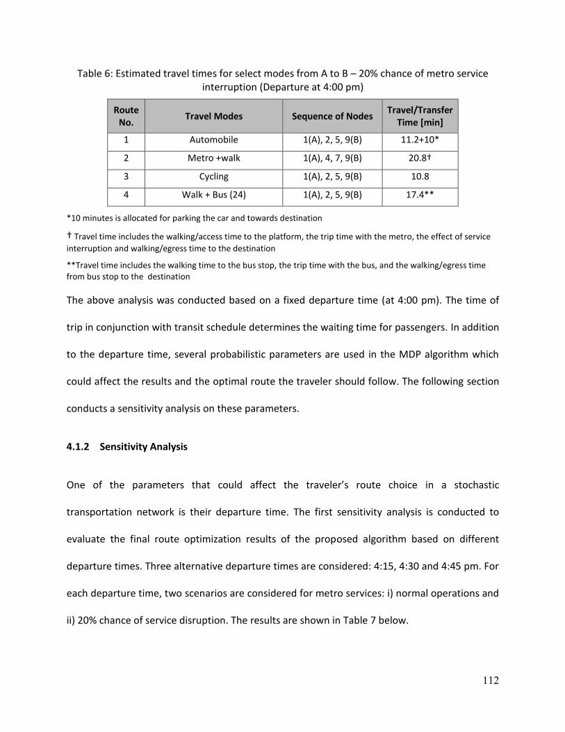
112
Table 6: Estimated travel times for select modes from A to B – 20% chance of metro service interruption (Departure at 4:00 pm)
Route No.
Travel Modes Sequence of Nodes Travel/Transfer
Time [min]
1 Automobile 1(A), 2, 5, 9(B) 11.2+10*
2 Metro +walk 1(A), 4, 7, 9(B) 20.8†
3 Cycling 1(A), 2, 5, 9(B) 10.8
4 Walk + Bus (24) 1(A), 2, 5, 9(B) 17.4**
*10 minutes is allocated for parking the car and towards destination
† Travel time includes the walking/access time to the platform, the trip time with the metro, the effect of service
interruption and walking/egress time to the destination
**Travel time includes the walking time to the bus stop, the trip time with the bus, and the walking/egress time from bus stop to the destination
The above analysis was conducted based on a fixed departure time (at 4:00 pm). The time of
trip in conjunction with transit schedule determines the waiting time for passengers. In addition
to the departure time, several probabilistic parameters are used in the MDP algorithm which
could affect the results and the optimal route the traveler should follow. The following section
conducts a sensitivity analysis on these parameters.
4.1.2 Sensitivity Analysis
One of the parameters that could affect the traveler’s route choice in a stochastic
transportation network is their departure time. The first sensitivity analysis is conducted to
evaluate the final route optimization results of the proposed algorithm based on different
departure times. Three alternative departure times are considered: 4:15, 4:30 and 4:45 pm. For
each departure time, two scenarios are considered for metro services: i) normal operations and
ii) 20% chance of service disruption. The results are shown in Table 7 below.

113
Table 7: Estimated travel times (A to B) for different departure times
Metro Service
Travel Modes Sequence of
Nodes
Travel/Transfer Time [min]
Departure
at 4:15 pm
Departure
at 4:30 pm
Departure
at 4:45 pm
Normal
service
Driving 1(A), 2, 5, 9(B) 11.2+10 21.2 21.2
Metro + Walk 1(A), 4, 7, 9(B) 9 10 7
Cycling 1(A), 2, 5, 9(B) 10.8 10.8 10.8
Walk + Bus (24) 1(A), 2, 5, 9(B) 17.4 18.4 21.4
Service
interruption
(0.2
probability)
Driving 1(A), 2, 5, 9(B) 21.2 21.2 21.2
Metro + Walk 1(A), 4, 7, 9(B) 20.8 22 19
Cycling 1(A), 2, 5, 9(B) 10.8 10.8 10.8
Walk + Bus (24) 1(A), 2, 5, 9(B) 17.4 18.4 21.4
As it can be seen in Table 7, the departure time affects the estimated travel times of the trips
made via the alternative routes with metro or the bus. As expected, when metro is operating
normally, the optimal route from A to B is by using metro. However, when there is service
interruption, using a BIXI® bicycle represents the fastest route to get to destination. If cycling is
not an option for the traveler, depending on the departure time, the metro or bus routes
become the alternative solution. For example, if the traveler starts from A at 4:15 or 4:30pm,
the optimal route is given by the bus line on Sherbrooke. But, if the traveler departs after
4:45pm, the metro would provide the fastest route (assuming that cycling is not an option for
the traveler).
Table 7 also provides the impact of metro service interruption in this hypothetical travel
scenario. It can be seen that the metro service interruption could increase the travel time of
this mode by 120%. Additional sensitivity analysis is conducted on testing different values of
metro service interruption probability, when this mode would become the second alternative

114
route. Figure 9 presents the changes in estimated travel time using metro under different
probabilities of having a service interruption. It can be seen that, for departures at 4:00 pm and
when the probability of metro service disruption is higher than 13%, the Bus alternative
becomes the optimal route to move from A to B.
Figure 9: Travel time impact due to different probability values of service interruption at Metro
(Departure 4:00 pm)
Similar sensitivity analysis can be conducted on different probabilities of bicycle availability at
BIXI® stations and its effect on the optimal route. Figure 10 presents the estimated travel times
for using the bicycle mode using different availability probability values. It can be seen that if
there is a 50% chance of no bicycles available at the station, the expected travel time increases
to nearly 15 minutes, which is comparable the expected travel time by bus. Depending on the
convenience level of travelers and their value of time, using the bicycle may not be an option
for them. Figure 10 also shows the expected travel time from A to B, under different
probabilities of observing peak-period traffic congestion. Similarly, as explained above, these
travel times include a flat 10-minute time for parking and walking to destination. On the other
0
5
10
15
20
25
0% 5% 10% 15% 20%
Trav
el t
ime
fro
m A
to
B [
min
]
Probability of Service Interruption
Metro Bus (24)
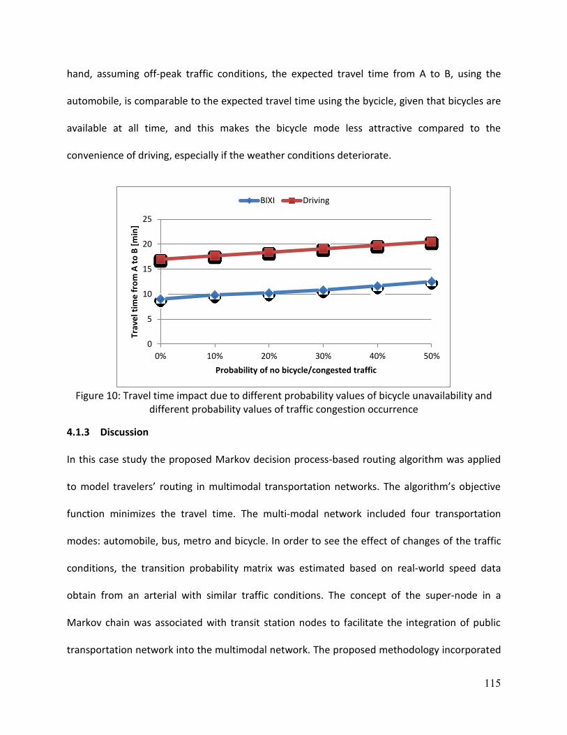
115
hand, assuming off-peak traffic conditions, the expected travel time from A to B, using the
automobile, is comparable to the expected travel time using the bycicle, given that bicycles are
available at all time, and this makes the bicycle mode less attractive compared to the
convenience of driving, especially if the weather conditions deteriorate.
Figure 10: Travel time impact due to different probability values of bicycle unavailability and
different probability values of traffic congestion occurrence
4.1.3 Discussion
In this case study the proposed Markov decision process-based routing algorithm was applied
to model travelers’ routing in multimodal transportation networks. The algorithm’s objective
function minimizes the travel time. The multi-modal network included four transportation
modes: automobile, bus, metro and bicycle. In order to see the effect of changes of the traffic
conditions, the transition probability matrix was estimated based on real-world speed data
obtain from an arterial with similar traffic conditions. The concept of the super-node in a
Markov chain was associated with transit station nodes to facilitate the integration of public
transportation network into the multimodal network. The proposed methodology incorporated
0
5
10
15
20
25
0% 10% 20% 30% 40% 50%
Trav
el t
ime
fro
m A
to
B [
min
]
Probability of no bicycle/congested traffic
BIXI Driving

116
transit schedule into calculations and was applied to a real-world network located in Montreal,
Quebec. The public transportation fixed schedule was used to compile the route node
parameters for the modeled network. The case study demonstrated the calculation procedure
of optimal routes for a traveler moving between two arbitrarily selected nodes in the network.
Several cases were tested by considering different operations conditions with a given
probability of congested traffic and/or service disruption for two of the available transportation
modes (Metro and Cycling). The results demonstrated the applicability of the proposed
algorithm to identify the fastest route to destination. It was shown that automobile travelers
can save up to 14 minutes of travel time by switching to another transportation mode (e.g.
metro, bus, or bicycle).
The case study clearly shows the applicability of the proposed algorithm in evaluating the
optimal route in a stochastic network and potential benefits as compared to shortest path
algorithm. The results showed that by accounting for some stochastic parameters of different
transportation networks, travelers could optimize their travel times when travel time delays
occur for specific transportation modes. In this case study, the availability of traffic data for the
study arterials was limited. Using wider range of speed data, for several days within the peak
period, could improve the traffic condition predictability. In addition, the probability of the
Bixi© bicycles being available could be more accurately estimated by using historical data
related to availability of bicycles at bike stations during rush hour throughout the study area.

117
4.2 Toronto case study
The first case study investigated one application of the proposed methodology in a small
network located within the downtown area of Montreal. In this section the MDP algorithm is
applied to model general travelers’ routing in a larger and more complex network of motorized
and non-motorized modes. The 45 km2 study area is located within the Greater Toronto Area
(GTA). The network includes more than 80 km of major roadways, including QEW and Gardiner
Expressway Highways (West of the CBD) and several major arterials within the Toronto CBD
area and is shown in Figure 11.
Figure 11: Layout of the study area, roadway network and select transportation modes (Source: Google Earth)
Go Train Subway Tram/Bus Bicycle Station Study Area
B
A

118
The boundaries of the study area are limited to Islington Avenue on the west, Bay St on the
east, Lakeshore Blvd on the south and Bloor St on the north. The selected area with multiple
transportation facilities (i.e. commuter trains, street cars, buses, subway and bicycle paths)
enabled us to better model the stochastic behavior of a transportation networks and to
evaluate the performance of proposed methodology in more realistic network.
The proposed method is used to find the optimal route for traveling between two arbitrarily
selected node (marked as A and B in Figure 11) by using private and public transportation. This
is a typical route for commuters living outside the City of Toronto. Travelers might combine
carpooling parking lots and the commuter trains. The analysis includes the peak period and
captures the heavy congestion along major highways (QEW and Gardiner Express) connecting
the GTA suburbs to downtown Toronto. During the rush hour periods, heavy traffic on the EB
highway/arterials towards downtown Toronto could be expected. The case study considers the
stochastic traffic conditions along the roadways within the study network. Travel time along
these roadways would change according to different traffic conditions.
4.2.1 Network Model
The network is modeled based on the methodology presented in Chapter 3. In total, 34 Nodes
and 58 links, to represent intersections and arterials, are identified in the study network. Figure
12 and Figure 13 present schematic of the model with the created node and link numbers
respectively. Nodes for the arterials represent the intersection of two streets. For Gardiner Exp.
nodes represent intersection of the exit ramp with the crossing street. If there is no exit
available (e.g. Gardiner Exp. at Bathurst St), no node is created (See Figure 12).

119
Figure 12: Schematic model of the nodes/node numbers within the network
The direction of traffic was considered when creating the links and separate links are created
for each direction of traffic along arterials related to the study area. However, not all the
bidirectional links are represented (See Figure 13).

120
Figure 13: Schematic model of the links/link numbers within the network
In addition eight bus/tram lines, two subway lines and one commuter train route were coded in
the model. The time-tables of the commuter train, tram/bus and subway at each station are
integrated into the transit model. Travel time information for transit modes is evaluated using
their regular daily schedule. The waiting time for next transit service is estimated based on
original departure time and estimated arrival time of individual traveler at each station/top.
Details regarding modeling the public transit lines are provided later in this section. Bicycle
sharing facilities near different nodes are also integrated into the network. Travel time for
bicycles/pedestrians on each link each are calculated based on typical average speeds used in
similar studies conducted by FHWA 2006.
In order to estimate the travel time along the network links under different traffic conditions, a
microscopic computer model of the study network was implemented using AIMSUN (Advanced

121
Interactive Microscopic Simulator for Urban and Non-Urban Networks). This software package
is a proprietary microscopic simulator that can model traffic conditions of real-world traffic
networks on a computer. The behavior of every single vehicle is continuously modeled
throughout the simulation using several driver behavior models (e.g. car-following, lane-
changing, gap-acceptance, etc.). AIMSUN is capable of performing microscopic and mesoscopic
simulation as well as hybrid simulation, allowing modeling of large areas while focusing on the
areas that require detailed traffic analysis. The reason for using AIMSUN in this case study is the
ability to easily import and edit GIS files as the first step in developing the model, as explained
here after.
In order to model the study area in AIMSUN, the following tasks were conducted:
1. The base geometry skeleton was developed by importing a GIS map of the study area in
AIMSUN. The GIS maps from Land Information Ontario (LIO) (See Figure 14) was used
which included key geometry attributes, i.e. number of lanes, road types, street names
and speed limits in multiple datasets. These datasets were appropriately merged into
one dataset based on a common identifier and joined with the road network map using
ESRI ArcGIS software;
Study Area

122
Figure 14: GIS network acquired from LIO and the study area in this project
2. The study area network with key attributes was imported in AIMSUN for development
of the base geometry. The model was then refined by using Google Maps and Google
Street View to make necessary changes regarding the geometry/number of lanes for all
roadways within the model. Figure 15 shows the network model in AIMSUN;
Figure 15: Study area modeled in AIMSUN
3. The actual traffic demand as well as traffic signal timings was coded in the model.
Separate traffic demand was available for a 4-hour period between 15:00 and 19:00. In
order to create free-flow and congested scenarios, the simulation was conducted for a
4-hour period (15:00 – 19:00) with available hourly demands. A half hour warm-up
period was used for the simulation. The microscopic model was calibrated using real
data collected during PM peak period for major arterials and QEW highway (traffic
counts, speed and travel time data). In order to account for the stochastic nature of

123
vehicle arrivals, five simulation runs with distinct random seeds were conducted. The
average of five replications was used as the final result.
4. The simulation results were stored in a SQLITE database file by AIMSUN. The output was
in the form of a table and included Section IDs, time intervals, and simulated travel
time/speeds. Each section ID in AIMSUN corresponds to one link in the modeled
network. SQL code was used to extract travel time and speed data for the required links
within the network from the SQLITE database. The data were imported into Excel from
SQLITE. A Visual Basic code was developed to import the results into a template created
in an Excel worksheet. Link travel times were assigned to corresponding arterials and
highway sections of the study area. (See Appendix A)
The simulation results were used to estimate the link travel times on Gardiner Expressway and
major arterials in the network under different traffic congestion levels. Travel times for all the
links were aggregated for 30 minute intervals within the 4-hour simulation period (3:00 – 7:00
pm). It was expected that during the first hour of simulation no congestion forms within the
network and therefore the estimated travel time during the first hour was considered as the
off-peak travel time. The simulation results for later hours within the simulation period were
also analyzed to estimate the travel times corresponding to the peak and congested traffic
conditions along each link.
4.2.2 Model Calibration
The control data used to calibrate the model was comprised of volume and speed data. The
volume data was compiled from a mix of counts from different detectors. Speed data was

124
collected for Gardiner Expressway, Lake Shore Boulevard and major arterials. For this study
area GPS based speed information from proprietary data accessible via private data collection
source was used. Signal timing plans were another important part of the model’s calibration
and was available from the municipalities with jurisdiction in the study area.
Driving behaviour
Driver behaviour is calibrated in four different categories within AIMSUN. The first category is
the model’s experiment properties. This is where the simulation step and reaction times are
calibrated. These two parameters are tied together in that the reaction time must be a multiple
of the simulation step. The simulation step and reaction time were adjusted to calibrate the
overall speeds and level of congestion on the highway and major arterials.
The second category is the section properties. The section properties are used to calibrate the
operation at on-ramps by adjusting how cooperative vehicles are with merging vehicles, the
distance over which that they will cooperate, and the distance over which vehicles will merge
into traffic. The section properties are also used to set speed limits.
The third category is the node properties. The node properties are used to calibrate how
vehicles will react to upcoming turns in their path. Each turn has two variables that define the
limits of three zones upstream. In the first zone, vehicles are unaware of the upcoming turn. In
the second zone, vehicles recognize the upcoming turn but will still make lane choice decisions
based on speed advantages. In the third zone, the vehicles will make whatever lane changes
necessary; even if they must slow down to do so. These parameters are key to calibrating traffic

125
operation at off-ramps and were adjusted in the model to reflect levels of congestion observed
in the speed data collected.
The fourth category is the vehicle properties. This is where characteristics such as speed
acceptance, maximum desired speed, and acceleration/deceleration curves are defined for
each vehicle type (e.g. cars, light trucks, heavy trucks, etc.).
The visual observation of the model was completed under different simulation scenarios to
ensure that the model overall is operating as expected and that driving behavior (merging, lane
changing, speed reduction, queue formation, etc.) is reasonable.
Volume
Traffic volume calibration involves comparing average traffic volumes generated from the
simulation model against the observed traffic volumes. The Geoffrey E. Havers (GEH) statistic
formula is used for this comparison. The GEH statistic is an empirical formula similar to chi-
square test that is used in traffic modelling to compare two sets of traffic volumes. GEH
statistics can be used as an acceptance criterion for travel demand forecasting and model
calibration as shown in Equation (7):
𝐺𝐸𝐻 = √2(𝑀−𝐶)2
𝑀+𝐶 (7)
Where, M is the hourly traffic volume from the model and C is the hourly volume from the
traffic count.

126
For calibrating traffic models in the "base case" scenario, according to the FHWA (2004)
guidelines for microsimulation modelling, a GEH of less than 5.0 for 85% of the links is
considered an acceptable match between the modelled and observed hourly volumes. In this
model, volumes of all major arterials and Expressway within the network were considered for
calibration. The calculated GEH for 90% of the volumes were less than 5.0 which shows that the
model is well calibrated in terms of traffic volumes. Figure 18 shows the calculated GEH
statistics for the model.
Figure 16: GEH Statistics Calculations for the modeled study area
Speed
Speed calibration was done for highway and major arterials. Speed profiles were constructed
from the GPS data and compared with outputs from the model. The GPS data is aggregated
based on changes in road cross-sections, resulting in a step-graph. The modeled speeds are

127
plotted in two forms: (1) as a step-graph based on AIMSUN’s section divisions and (2) a smooth
line-graph based on detectors spaced every 100m. Figure 17 shows a sample speed profile for
Gardiner Expressway.
Figure 17: Speed profile used for calibration – Gardiner Expressway
4.2.3 Traffic Conditions and Transition Probabilities
The proposed MDP methodology incorporates transition probabilities which denote the
probability that traffic conditions change from one node to another node within the network. In
order to estimate the probability of observing different traffic conditions and the related
transition probability matrix, real-world traffic speed was used to identify different traffic
conditions related to the study network. The following tasks have been performed to build the
transition probability matrix for the MDP methodology:
_______ GPS Speed
_______ Section Speed
______ Detector Speed
_______ GPS Speed _______ Section Speed ______ Detector Speed

128
1. Traffic speed data collected for two different directions along four major arterials in
Toronto during the 4th week of September 2012 was available. The average speed data
from GPS equipped vehicles was aggregated over 15-minute period intervals. Speed
data was available for about 50 kilometer length of major arterials was analyzed.
2. Speed graphs for 15-minute time intervals where created and analyzed to better
understand the range of changes in the average speed data along each
corridor/direction. The analysis was done for the period between 14:00 and 19:00 and
for all weekdays, the weekend data were excluded. Figure 18 shows a sample of such
graph for the northbound direction of one section along Dufferin St.
Figure 18: Sample of 15-minute interval average speed profile along Dufferin St. (NB)
3. Based on the observations from the speed graphs, outlier days/locations were removed
from the analysis. For example, in case Dufferin St. speed graph shown in Figure 18, the
average speed data related to “day 1” was identified as an outlier (with a different
trend compared to the other days) and therefore was not considered for the
0
10
20
30
40
50
60
70
Spe
ed
(K
m/h
)
Time of Day
Average Weekday Speed - Dufferin St. NB
Day 2
Day 3
Day 4
Day 5
Day 1

129
calculation. Day 1 was considered to be an outlier because more than 70% of the data
points were outside the 95% confidence interval of the other four days.
4. The collected speed values were divided into three arbitrary ranges to represent three
types of traffic conditions: A) off-peak: speed > 40km/h; B) peak: 20< speed <= 40
km/h; and C) congested: speed <= 20km/h.
5. A visual basic program was developed to calculate the elements of transition
probability matrix by applying the methodology described in Chapter 3. The probability
of observing a change in traffic conditions was estimated based on number of changes
in the average traffic speed from one traffic condition range (defined above) to another
during each 15-minute interval. This calculation was done based on weekday data
(excluding weekend and outlier) and for each direction of travel along each arterial.
6. The calculated probability matrices of arterials were compared for the directions of
traffic movement related to this study (northbound and eastbound). Final transition
probability matrix was calculated by averaging the corresponding elements of each
probability matrix of arterials and is shown in Table 8.
Table 8: Transition Probability Matrix (Arterials)
Future Traffic State
Current Traffic State A B C
A (off-peak) 0.86 0.14 0.00
B (peak) 0.11 0.86 0.03
C (congested) 0.03 0.22 0.75
7. Each row in Table 8 represents the probability of the change in traffic condition from
initial state (Rows: A, B and C) to another state (Columns: A, B and C). Based on this

130
table, the probability of the traffic conditions to improve from level C to level A and B is
0.03 and 0.22 respectively. Similarly, the probability of traffic condition level B to be
improved to level A is 0.11. There is also 3% chance that traffic condition would
deteriorate from level B to level C. Moreover, the probabilities of traffic condition levels
A, B and C to remain at the same level are 0.86, 0.86 and 0.75 respectively.
As it can be seen in Table 8, the sum of probabilities for traffic change (each row) is
equal to one. However, this relationship does not apply to the columns of this table. On
the other hand, the numbers along columns of the table does not represent the same
probability relationship between two states. The transition probability numbers are only
applicable if the initial traffic state is chosen form rows and the future traffic state is
selected from one of the columns.
8. The study area in this study includes one major east-west Highway (QEW) that connects
Toronto to the west of the province. It should be noted that the changes in traffic flow
parameters on highways (e.g. speed, density, shockwave speed) is different than those
on arterials, therefore the probability of changes in traffic state is also different and
should be considered in the analysis. For the purpose of this study, since the
aggregated speed data was not available for QEW highway, a parallel highway (401)
was used as reference for evaluating the transition probability matrix along highway
section.
Spot speed data on two different sections of Highway 401 was available for one day
(May 13 2011). Speed values were aggregated for 1-min periods between 15:00 and
19:00 on the count day. The same process as for the arterials was used to estimate the

131
probability of change in the speed on vehicles on the EB direction of the highway, as per
the study area. The collected speed values were divided into three arbitrary ranges to
represent three types of highway traffic conditions: A) off-peak: speed > 70 km/h; B)
peak: 50< speed <= 70 km/h; and C) congested: speed <= 50 km/h.
The final probability matrix was built by using the average probabilities for each change in
traffic state on highway 401. Table 9 presents the results:
Table 9: Transition Probability Matrix (Highway)
Future Traffic State
Current Traffic State A B C
A (off-peak) 0.71 0.29 0.00
B (peak) 0.12 0.59 0.29
C (congested) 0.00 0.17 0.83
9. In order to have similar transition probabilities for the whole network, the average
probabilities between the two matrices are used as the final transition probability
matrix in the MDP algorithm (see Table 10)
Table 10: Transition Probability Matrix (Study Network)
Future Traffic State
Current Traffic State A B C
A (off-peak) 0.78 0.21 0.00
B (peak) 0.12 0.72 0.16
C (congested) 0.02 0.19 0.79
The initial transitions probability matrix can be created by using arbitrary probability
values and based on the available departure time. Depending on the departure time and

132
its observed traffic conditions, a higher probability should be assigned to related traffic
state. For example, for the beginning of peak period, it is assumed that traffic state B
(peak) has a higher probability compared to the other two states. Therefore, the
arbitrary probability matrix presented in Table 11 can be used:
Table 11: Initial probability matrix when departure time is at the beginning of peak period
A B C
25% 50% 25%
4.2.4 Public Transit Network
The study area included the following transit modes/lines (as shown in Figure 19):
1. Go Transit Lakeshore east train, with 3 station within the study network (i.e. Mimico,
Exhibition and Union);
2. Subway yellow line 1 (Yonge-University-Spadina), where 5 stations were included in the
study area (i.e. Union, St Andrew, Osgoode, St Patrick and Queen’s Park);
3. Subway green line 2 (Bloor-Danforth), where 15 stations starting from Islington on west
to St George St were included in the study network;
4. Bus line 6, with 5 stops on Bay St (i.e. at Front, Queen, Dundas, College and Wellesley
Streets);
5. Bus line 142 (express), with 4 stops on University St (i.e. at Queen, Dundas, College and
Wellesley Streets);
6. Streetcar line 501/Bus line 301, with 3 stops along Queen St (at Bathurst, Spadina and
University Streets);

133
7. Streetcar line 505, with 3 stops along Dundas St (at Bathurst, Spadina and University
Streets);
8. Streetcar line 506/Bus line 306, with 3 stops along College St (at Bathurst, Spadina and
University Streets); and
9. Streetcar line 511, with 3 stops along Bathurst St (at Queen, Dundas and College
Streets).
The transit schedule for each line at each station/stop was derived from Toronto Transit
Commission (TTC) website and is provided in Appendix B. Travel time on each link between
each two steps within the network was then calculated based on the scheduled times at
each station. In addition, any applicable waiting time was also calculated based on the
difference between estimated traveler’s arriving time at station and scheduled transit time
and was added to travel time of related link.

134
Figure 19: Transit network within the study area
The study area also includes 20 bike sharing stations of BikeShare Toronto. It was assumed that
during the analysis, the bicycle docking stations have at least one available bike to rent or one
available spot to return the bicycle. The travel time for the links by using bicycle mode was
estimated based on the length of the link and by applying an average speed of 12 km/h for
bicycles. An additional one minute was allocated for docking and undocking the bicycles at each
station. The average walking speed of 5 km/h was used to calculate the walking time on each
link.
1
B
Go Transit train
Subway line 1
Subway line 2
Tram/Bus (301/501,306/506,505,511)
Bus line 6 & 142
Bicycle Station
Destination
1
301/ 501
306/ 506
505
511
2
6 142

135
4.2.5 Routing Constraints
In order to improve the efficiency of the routing algorithm and to better represent the actual
behavior of passengers, the following constraints/assumptions were considered in developing
the algorithm:
1. The maximum number of mode transfers (e.g. car to bus, bus to walking, etc.) is limited
to two, to represent more realistically the expected behavior of commuters.
2. In regards to private mode (cars), mode change is only allowed from car to other
transportation modes (and not vice versa). In this case, a transfer time of 5 to 15
minutes (variable based on the location) is considered for parking the vehicle and
arriving at the station/stop. For example, in case of commuter train parking lots, which
are outside the CBD, this transfer time is smaller than the expected transfer times for
parking within the CBD area (i.e. roadside parking).
3. The expected average transfer time for accessing bicycle-sharing docks is two minutes.
4. All prohibited turn movements at various intersections are considered in the algorithm.
5. For transfers between the commuter train and other transit modes at the downtown
central station (Union station) an average five-minute transfer time is assumed.
4.2.6 Analysis Results
The proposed algorithm was applied to find the optimal path between the arbitrarily selected
points A and B. A starting time of 17:00 was used as reference time for travel time calculations.
A Visual Basic (VB) program was developed to implement the routing model described in the

136
previous chapter and to estimate the optimal route. The VB code used recursive function
technique to process the MDP algorithm (See Appendix C).
Table 12 shows the results of estimating the optimal and select alternative routes of the
hypothetical trip made by a commuter between A and B. It is assumed that traveler uses his
own private vehicle to depart from A. Since the algorithm only identifies the optimal path, its
implementation in the VB code was adjusted to obtain, for comparison purposes, two
alternative paths presented in the following tables (Route No. 2 and 3).
Table 12: Estimated travel times for select routes from A to B
Route No.
Transit Modes Sequence of Nodes (See
Figure 20-Figure 22)
Travel Time [min]
1 Car, Subway, Bike/Walk A,2,3,4,5,11,18,25,B 30
2 Car, Walk A,1,13,20,21,22,23,24,B 61
3 Car, Go Train, Subway, Walk A,1,6,28,21,22,23,24,B 34
According to Table 12 the following observations can be made regarding the results:
1. The optimal route for traveler (minimum travel time) is to drive north and then east
along Bloor St, up to Bathurst St. and then take the subway to University St. Then, they
can use bicycle or they can walk towards destination (See Figure 20). The total travel
time of this path is 31 minutes, compared to 61 minute estimated time for using car
only (driving from A to B).

137
Figure 20: Traveler’s optimal route
2. The second best option is to take the commuter train up to Union Station, and then
switch to subway NB up to College St. Then, they can walk to destination (See Figure
21). Total estimated travel time is this scenario is 34 minutes.
Driving Car Subway Bicycle Route /Walk

138
Figure 21: Second alternative route
3. Estimated travel time for driving along Gardiner highway EB and then University St NB
(as shown in Figure 22) is about an hour, which is almost twice the time along the
optimal route by using public transit. This is true during the congested traffic state.
However, in case of normal traffic conditions (peak period) the estimated travel time for
this route is 30 minutes.
Driving Car Go Train Subway Bicycle Route /Walk

139
Figure 22: Preferred route under normal traffic condition
4.2.7 Sensitivity Analysis
In order to evaluate the effect of the stochastic parameters on the MDP algorithm results, a
sensitivity analysis is conducted. The effect of arbitrary selected ranges of travelling speed, to
represent different traffic conditions is evaluated. Initially, the following ranges of speed values
are used to represent the following conditions: A) off-peak: speed > 45km/h; B) peak: 30<
speed <= 45 km/h; and C) congested: speed <= 30km/h. The estimated travel times for previous
routes are calculated using the proposed algorithm and results are shown in Table 13.
Table 13: Estimated travel times for select routes from A to B (revised transition probabilities)
Route No.
Transit Modes Sequence of Nodes (See
Figure 20-Figure 22)
Travel Time [min]
1 Car, Subway, Bike/Walk A,2,3,4,5,11,18,25,B 31
2 Car, Walk A,1,13,20,21,22,23,24,B 53
3 Car, Go Train, Subway, Walk A,1,6,28,21,22,23,24,B 34
Driving Car Walk

140
It can be seen that the expected travel time using the automobile mode could change by about
10% for different routes. However, the optimum route and the second preferred route do not
change.
Additionally, the limits of speed ranges representing different traffic conditions are decreased
to the following values: A) off-peak: speed > 30km/h; B) peak: 15< speed <= 30 km/h; and C)
congested: speed <= 15km/h. Updated travel times for preferred routes are shown in Table 14.
Table 14: Estimated travel times for select routes from A to B (revised transition probabilities)
Route No.
Transit Modes Sequence of Nodes (See
Figure 20-Figure 22)
Travel Time [min]
1 Car, Subway, Bike/Walk A,2,3,4,5,11,18,25,B 31
2 Car, Walk A,1,13,20,21,22,23,24,B 54
3 Car, Go Train, Subway, Walk A,1,6,28,21,22,23,24,B 34
The results show that there is minimal increase in travel time for route no. 2, by 1 minute.
Nevertheless, the optimal and the second preferred route do not change. While under the
tested case study the sensitivity analysis does not show significant impact on the optimal route,
it can be seen that this model is able to capture such variations, and depending on the
complexity of the network one can use the model to identify optimal routes under different
traffic conditions.
The above analysis was conducted by applying similar transition probability matrices for
arterials and highways. This was done using the average of two transition probability matrices
(Table 10). As discussed in Section 3.5, the traffic pattern and changes in traffic speed may be
different on arterials and highways and separate transition probability matrices may be used

141
for different roadways within the network. To study the effect of this change, additional
analysis was conducted to identify the optimum route by using the transition probability
matrices for corresponding link types (i.e. Table 8 for arterials and Table 9 for highway) and the
results are summarized in Table 15.
Table 15: Estimated travel times for select routes from A to B (Different transition probability Matrices for arterials and highway)
Route No.
Transit Modes Sequence of Nodes (See
Figure 20-Figure 22)
Travel Time [min]
1 Car, Subway, Bike/Walk A,2,3,4,5,11,18,25,B 28
2 Car, Walk A,1,13,20,21,22,23,24,B 55
3 Car, Go Train, Subway, Walk A,1,6,28,21,22,23,24,B 34
The results show minor improvements in estimated travel time for the optimum (28 min vs. 31
min). This is due to the smaller chances of transitioning to congested traffic condition in the
transition probability matrix for arterials as compared to the average transition probability
matrix for the whole network.
4.2.8 Discussion
The proposed MDP algorithm was applied to a real world transportation network located within
the Greater Toronto Area to find the optimal path for a traveler between to arbitrary points.
The studied multi-modal network included Commuter train, Bus, Street car, Subway, Bicycle
and Automobile modes. The transit network schedule was modeled using the Super node
approach presented in the previous sections. In order to account for changes in traffic
conditions, transition probability matrices were evaluated using real world speed data along
several roadways in the Toronto City. The proposed routing algorithm successfully identified

142
the optimal (shortest) route for a traveler moving between two arbitrarily selected locations in
the network, using different travel modes. A sensitivity analysis was conducted to demonstrate
the ability of the model to capture the effect of probabilistic parameters used for the route
estimation. It was also shown that the proposed methodology can realistically account for the
stochastic properties of traffic conditions along different types of transportation facilities. While
there were some limitations of the data source (only one highway segment was used to collect
highways-specific transition probability matrix) there was sufficient data to demonstrate how
using different transition probability matrices for different type of links (i.e. arterials vs.
highways) can lead to different outcome (i.e. optimal path). It is expected that if a more
heterogeneous network is tested (i.e. different types of facilities and associated probability
matrices) using specific matrices by road type would lead to more realistic modeling results
when an aggregated transition probability matrix is used.
In this case study first a network wide transition probability was applied for route optimization.
A sensitivity analysis was conducted to see the effect of applying separate transition probability
matrices for arterial and highway corridors. Given that in a large transportation network there
is a high degree of heterogeneity in terms of traffic conditions along different roadway types at
any given time, the reliability of the methodology could be further improved by utilizing
different transition probabilities for different sections of a large network.

143
4.3 Longueuil case study
The 2-km long study area is located on a corridor between the Champlain and Victoria bridges,
in Longueuil, Quebec. The two-way, three lanes each direction arterial, Boulevard Taschereau,
(henceforth referred to as the major street) crosses five local streets (minor approaches), see
Figure 23. The major street is used on both directions by several bus lines from RTL (Reseau de
transport de Longueuil). All bus stops are placed at the stop line of each intersection with the
minor streets (i.e. near-side bus stops). In this study the west bound approach of the major
street, starting from Churchill Blvd, is considered as the regular path for RTL bus line number 4.
This bus line originates from the Longueuil terminal, heading west towards Cornwall and
Maricourt and has five stops within the study area and cannot be skipped.
The reason for selecting this particular segment is that it is a straight section of a major
roadway (134) that further downstream merges into highway 15. In addition, there are several
arterials and minor streets (e.g. Rue Victoria, Rue de Mont Royal) available for rerouting the
busses in case of congestion along the major road. The average spacing between bus stops is
about 400 m. The extra distance that bus would travel in case of rerouting ranges between 200
and 700 meters.
In this case study all buses travel between nodes 1 and 5 (as shown in Figure 24), which
represent the beginning and the destination nodes, respectively. If rerouting via minor roads is
necessary, the stops can be relocated downstream of the intersection either on the major
street or on the minor street, depending whether, in order to reach the next stop, the bus will
get back on the predetermined route or will continue on an alternative route , respectively. For
example, a bus may detour via Mont Royal Street in order to advance from node 2 to node 3. If

144
the bus resumes its predetermined route on the major road then, in order to service the stop at
node 3, it will stop on the major road downstream of the Charles Street intersection.
Figure 23: Layout of Study Area (Source: Google Maps)

145
Figure 24: Alternative scenarios: lane closures in the network
Figure 25: Bus routes: nodes and links

146
To evaluate the effectiveness of the proposed approach in the real world, traffic demand data
and phasing times for signal controllers of intersections were collected from Quebec Transport
Ministry and bus schedule and passenger count data was available through the local public
transit agency, Reseau de Transport du Longueil (RTL). The bus schedule is used to generate bus
fleet for microscopic simulations and also in model calibration to ensure buses arrive at
consecutive bus stops according to their schedule. The passenger count data were used in the
model as number of boarding/alighting for buses at each stop and to calculate their dwell time.
Based on field observations, the afternoon peak hour demand on the major street varies
between 800 and 2000 veh/h on each direction during the three peak hours between 15 and
18. Also, the volume of cars on minor approaches is estimated at 200 veh/h.
The network, i.e. arterials and minor streets presented in Figure 24, was modeled and calibrated
in a microscopic simulator, VISSIM (PTV America 2011). VISSIM is a microscopic, time-step and
behavior-based simulation model capable to simulate mixed vehicular traffic including public
transportation operations. It is being used for more than two decades by researchers and
practitioners in various transportation applications. In this study the latest available version
was used, VISSIM 5.2. The reason for using VISSIM in this case study is the ability to easily
define and work with transit lines/routes and bus stops within the model.
4.3.1 Model Calibration
The model was calibrated based on the available traffic demand from MTQ at several
intersections along Taschereau Blvd. The simulated traffic volumes were compared with vehicle
counts to make sure the FHWA (2004) guidelines for micro-simulation modelling (Equation 7), a

147
GEH value less than 5.0 for 85% of the links is met. A summary of calculated GEH statistics for
different locations along the major road is presented in Figure 26. Speed data at the study
corridor were not available to be used for the calibration.
.
Figure 26: GEH Statistics Data
4.3.2 Experimental Analysis
For illustrative purposes, in this study we assume that major street is characterized by one of
the five different traffic conditions. Each traffic condition corresponds to a different state in the
associated Markov system. One of the states represents free-flow operating traffic conditions
under which bus operations on the pre-determined bus routes are not affected. The other five
states correspond to five different traffic congestion levels based on possible lane closures
scenarios as shown in Figure 24 and defined below:

148
Scenario 1: One EB traffic lane is closed on Taschereau Boulevard, west bound at the
end of the study corridor between Regent and Lawrence Streets (nodes 4 and 5 in Figure
25).
Scenario 2: Two EB traffic lanes are closed to traffic on Taschereau Boulevard, west
bound between Regent and Lawrence Streets.
Scenario 3: One EB traffic lane on Taschereau Boulevard, between Margaret and Regent
Streets is closed to vehicles (nodes 3 and 4 in Figure 25).
Scenario 4: Two EB traffic lanes are closed to traffic on Taschereau Boulevard, west
bound between Margaret and Regent Streets.
Scenario 5: Two EB traffic lanes on Taschereau Boulevard, between Charles and
Lawrence Streets are closed to traffic.
Each scenario was simulated in VISSIM for three hours using the same traffic demand input (See
Table 16). Each scenario was run with the same ten distinct random seeds, to account for
stochastic variations in the model and to allow for consistent comparison. Standard deviation
and standard error of ten travel times based on ten different random seeds were calculated at
different time stamps for each scenario. It was observed that the confidence interval for most
of the travel times of buses were below 10% except for a few cases. This can be explained by
the fact that due to inherent randomness of each simulation run, in certain instances buses may
be affected by additional delay due to random vehicle arrival at the traffic signal. Since the
simulated corridor is short, 2-km long, the impact of waiting an additional cycle length at one of
the intersections along the corridor may have a substantial effect on the accumulated travel
time on the links.

149
Table 16: Vehicle input volumes
Total Vehicle Flow
(Veh/h) Movement
Ratio (% of total
Flow) Approach/Simulation
Time
First
hour
Second
hour
Third
Hour
Taschereau West
bound 800 1600 2000
Through 80%
Right/Left Turn 20%
Taschereau West
bound 800 1600 2000
Through 60%
Right/Left Turn 40%
Churchill
Boul./Grande
Allée/Victoria St. 200 200 200
Through 60%
Right/Left Turn 40%
A total of 50 simulation runs were conducted. Average bus travel times were calculated from
each simulated scenario. A 𝑡-test analysis was conducted to determine if the difference
between average travel times estimated in alternative scenarios are statistically significant for
similar links. Table 17 shows the results of the tests that compare average travel time, in
seconds, of the base scenario – the scenario representing free-flow traffic conditions, μ0 and
the average travel time of buses in each of five traffic congestion alternative cases (𝜇𝑖 , where
𝑖 = 1 … 5). The null hypothesis tested is that the two average values are not significantly
different (𝐻0: 𝜇0 − 𝜇𝑖 = 0) at 95% confidence.
It can be seen in Table 17 that under certain traffic conditions, some links shows statistically
significant different average travel times at 95% confidence. For example, it was found that
there is a statistically significant difference between average travel times on link 7 when the
base scenario and scenario 4 are compared. Moreover, link no. 4 shows a statistically significant
150
difference for all simulated traffic conditions. This means that if buses are rerouted to travel
through links 4 and 7, there will be a significant saving in travel times under certain traffic
conditions. Furthermore, for other links, the t-test results show that statistically there is no
difference between average travel times estimated for alternative scenarios. This indicates that
these links may not have significant effect on the savings in travel time/costs, if the buses are
rerouted to travel through them to get to the destination. The optimal routing calculations
provided in the next section yield to the same conclusion.
It can be seen in Table 17 that link number 4 has the most significant results compared to the
base scenario. This can be explained that by creating traffic congestion on the links downstream
of link 4, the queuing condition occurs at upstream since the vehicles are not able to clear the
intersection and travel via the available downstream lanes. Therefore, the travel time on link 4
increases compared to alternative routes. Due to the relatively low congestion level created in
the network in scenarios 1-4 the other links did not show a statistically significant travel time
difference. By modeling more severe congestion conditions, scenario 5, much longer queuing
occurred upstream on link 4 and additional optimized paths were identified which are
presented in the following section.

151
Table 17: Results of the t-test analysis for the travel time difference
t-values for t-test (𝐻0: 𝜇0 − 𝜇𝑖 = 0; 𝑤ℎ𝑒𝑟𝑒 𝑖 = 1. .5)
Link no. Scen. 1 Scen. 2 Scen. 3 Scen. 4 Scen. 5
2 0.72 0.12 0.2 -1.5 -27*
4 -2.9* -2.8* -3.0* -6.6* -7.3*
5 -0.33 -0.83 -0.71 -4.3* -130*
7 -1.1 -0.78 -1 -8.1* -8.2*
* denotes statistically different means at 95% confidence (t-critical = 2.03)
4.3.3 Computation Results
The impact of the hypothetical traffic congestion scenarios defined above was evaluated
through the proposed adaptive routing methodology. In the proposed methodology, a penalty
(cost) is assigned in each step while moving from one node to another. Equation (5) is used to
estimate total penalties earned at the end node and decision is made based on minimized
penalties. In this study, the objective is to find the optimal route for which the total cost is
minimized. The reward for traveling from one stop to the adjacent one is calculated considering
both travel time and operating costs for buses. Based on a report released by Transport Canada
(2006), the value of time for passengers is estimated as $29.7 per hour (2003 $). Using the
latest annual report of American Public Transportation Association (2010), operating cost for
buses is calculated as $5 per kilometer (2008 $) which includes Vehicle Operations,
Maintenance, General Administration (Salaries and Wages, Materials and Supplies, Services)
and Purchased Transportation.
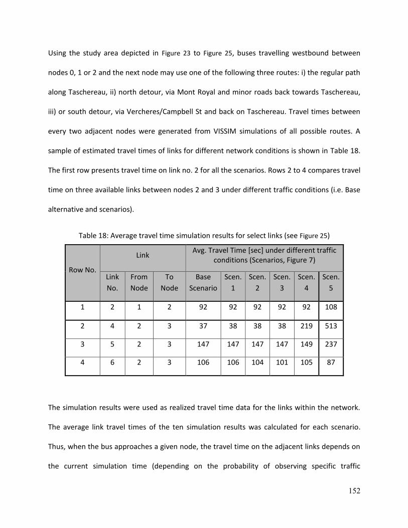
152
Using the study area depicted in Figure 23 to Figure 25, buses travelling westbound between
nodes 0, 1 or 2 and the next node may use one of the following three routes: i) the regular path
along Taschereau, ii) north detour, via Mont Royal and minor roads back towards Taschereau,
iii) or south detour, via Vercheres/Campbell St and back on Taschereau. Travel times between
every two adjacent nodes were generated from VISSIM simulations of all possible routes. A
sample of estimated travel times of links for different network conditions is shown in Table 18.
The first row presents travel time on link no. 2 for all the scenarios. Rows 2 to 4 compares travel
time on three available links between nodes 2 and 3 under different traffic conditions (i.e. Base
alternative and scenarios).
Table 18: Average travel time simulation results for select links (see Figure 25)
Row No.
Link Avg. Travel Time [sec] under different traffic
conditions (Scenarios, Figure 7)
Link
No.
From
Node
To
Node
Base
Scenario
Scen.
1
Scen.
2
Scen.
3
Scen.
4
Scen.
5
1 2 1 2 92 92 92 92 92 108
2 4 2 3 37 38 38 38 219 513
3 5 2 3 147 147 147 147 149 237
4 6 2 3 106 106 104 101 105 87
The simulation results were used as realized travel time data for the links within the network.
The average link travel times of the ten simulation results was calculated for each scenario.
Thus, when the bus approaches a given node, the travel time on the adjacent links depends on
the current simulation time (depending on the probability of observing specific traffic

153
conditions on those links). Transition probability matrix is formed based on the assumption that
the five different traffic conditions (i.e. free-flow, congestion scenario 1, 2, 3, 4 or 5) may occur
with the same probability through the network (𝑝𝑖𝑗=0.2). A Visual Basic code was written to
manipulate data and estimate the optimal route based on the proposed methodology (Figure
3). A recursive function is used in the code that accepts the beginning and destination nodes
and arriving time at beginning node as parameters, calculates the links travel times based on
the arrival time at nodes and calculates total cost by using Equation (5) for each chain of links
between beginning and destination nodes. The total cost is evaluated by summing up the
estimated travel time converted to cost and operating cost for the total distance traveled by
bus. The combinations of links that yield the minimum total cost are selected as optimal route
to be taken by the bus.
Table 19 shows select analysis results for the studied area. For example, under congested traffic
conditions caused by closure of two traffic lanes between nodes 3 and 4 (Scenario 4), if buses
arrives at 𝑛𝑜𝑑𝑒 1 at 𝑡 = 25𝑚𝑖𝑛, the regular path (links 1,4,7 and 10) remains the optimal route.
However, if the bus arrives at 𝑛𝑜𝑑𝑒 1 at a later time (i.e. 𝑡 = 80 𝑚𝑖𝑛) then the optimal route is
determined by links 1,6,7 and 10. The estimated cost savings are per passenger on the bus.
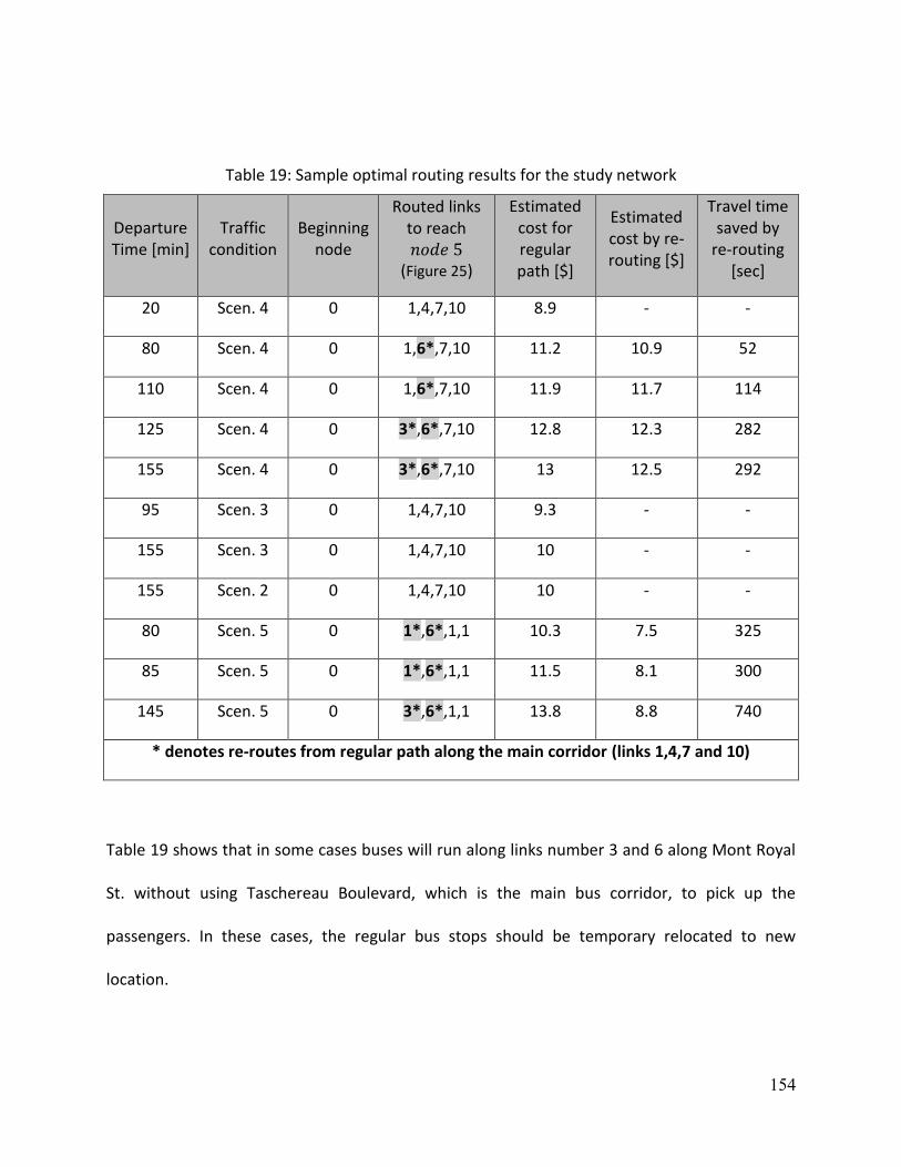
154
Table 19: Sample optimal routing results for the study network
Departure Time [min]
Traffic condition
Beginning node
Routed links to reach 𝑛𝑜𝑑𝑒 5
(Figure 25)
Estimated cost for regular path [$]
Estimated cost by re-routing [$]
Travel time saved by
re-routing [sec]
20 Scen. 4 0 1,4,7,10 8.9 - -
80 Scen. 4 0 1,6*,7,10 11.2 10.9 52
110 Scen. 4 0 1,6*,7,10 11.9 11.7 114
125 Scen. 4 0 3*,6*,7,10 12.8 12.3 282
155 Scen. 4 0 3*,6*,7,10 13 12.5 292
95 Scen. 3 0 1,4,7,10 9.3 - -
155 Scen. 3 0 1,4,7,10 10 - -
155 Scen. 2 0 1,4,7,10 10 - -
80 Scen. 5 0 1*,6*,1,1 10.3 7.5 325
85 Scen. 5 0 1*,6*,1,1 11.5 8.1 300
145 Scen. 5 0 3*,6*,1,1 13.8 8.8 740
* denotes re-routes from regular path along the main corridor (links 1,4,7 and 10)
Table 19 shows that in some cases buses will run along links number 3 and 6 along Mont Royal
St. without using Taschereau Boulevard, which is the main bus corridor, to pick up the
passengers. In these cases, the regular bus stops should be temporary relocated to new
location.

155
Although moving bus stops can be confusing for the riders, however, temporary relocation of
bus stops is being practiced in the city of Montreal by local transportation agencies. For
example, during special events, STM regularly cancels or relocates bus stops in the network.
This happens for example in cases of accidents along the urban routes, or due to heavy snow
falls during winter season. The STM mobile vehicles are responsible for posting necessary signs
and guidelines. These changes will also be reflected in the online schedule and all the drivers
will be informed by radio. The passengers will have to wait at new location to board the bus
and buses will not wait for potential passengers to arrive so there will be no significant changes
in their dwell time.
It can be seen in Table 19 that for some traffic conditions re-routing based on minimum cost
method is not necessary. Nevertheless, the proposed methodology can help transportation
operators to use flexible cost policies to manage their fleet and provide passengers with better
service when specific traffic congestion conditions occur in the network. Since the case study is
based on a small network with short distances, the savings in travel times are not considerable.
If a larger area of transit network is considered and modeled accordingly by applying the
proposed method to all bus lines, it is expected that total savings in the network would provide
considerably higher benefits to both, the travelers and the transit authority.
4.3.4 Sensitivity Analysis
The bus optimal path identified by the proposed algorithm given the study network depends on
several parameters. Due to changes in traffic conditions during the study period, one parameter
is the departure time of the bus and the initial traffic conditions. The results presented Table 19

156
show effects of assuming different departure times on the trip optimal cost, under different
traffic conditions. Since the results shown in Table 19 were based on total cost saving per
individual passenger, additional analysis is conducted to estimate the cost savings based on the
passenger occupancy of the bus. The estimations are done by assuming the average number of
passenger in the bus to be 10 and 20 persons, respectively and the results are summarized in
Table 20. It can be seen that when the average number of passengers in the subject bus
increases, total cost savings by rerouting the bus during congested traffic conditions would also
increase. This applies to only one bus line. The same estimation can be done for the whole fleet
and total estimated cost savings can be used for justifying the rerouting exercise.
Table 20: The effects of re-routing on trip cost-savings under different scenarios
Departure Time [min]
Traffic condition
Beginning node
Routed links to reach 𝑛𝑜𝑑𝑒 5
(Figure 25)
Cost saving by rerouting [$]
(10 passengers onboard)
Cost saving by rerouting [$]
(20 passengers onboard)
20 Scen. 4 0 1,4,7,10 - -
80 Scen. 4 0 1,6*,7,10 3 6
110 Scen. 4 0 1,6*,7,10 2 4
125 Scen. 4 0 3*,6*,7,10 5 10
155 Scen. 4 0 3*,6*,7,10 5 10
80 Scen. 5 0 1*,6*,1,1 28 56
85 Scen. 5 0 1*,6*,1,1 34 68
145 Scen. 5 0 3*,6*,1,1 50 100
* denotes re-routes from regular path along the main corridor (links 1,4,7 and 10)

157
4.3.5 Discussion
The Longueuil bus line case study investigated one application of the proposed methodology by
providing transportation operators with an overall situation of the system and its performance
and by assisting decision makers in their assessment to improve the efficiency of transportation
system. This case study applied the proposed MDP algorithm to estimate the optimal path a
bus should follow while maintaining the scheduled bus stops. An objective function was
defined to minimize the bus travel time by considering value of time and operating costs of the
fleet. The proposed methodology was applied to a 2-km long section of a bus line operating
along a 3-lane arterial, for which five different traffic congestion scenarios were tested. The
assumed scenarios represent one or two lanes closed to all traffic at two different locations
along the regular bus line. The simulation results for congestion conditions of scenario 4
showed that the travel time saved in several time intervals was in the range of 50 to 740
seconds. The sensitivity analysis showed that, depending on traffic conditions, the total cost
savings per bus (i.e. value of passenger lost time due congested conditions) can be as high as
$100, when an average of bus occupancy of 20 passengers is assumed.
This case study only considered one bus line and for a short section of their regular path. The
potential benefits of cost savings for transit agencies could be better evaluated by considering
several transit lines within their fleets and for a larger transit network. In addition, the traffic
conditions prediction could be significantly improved by using real-world traffic data collected
for the study arterials.

158
CHAPTER 5. CONCLUSION AND RECOMMENDATIONS
5.1 Conclusion
The research beforehand developed a novel routing procedure for multi-modal networks based
on graph theory and Markov Decision Process. The most important benefit of this routing
methodology stems from its application in a system optimization context. This is due to the
flexibility of the objective defined by the proposed procedure. Mainly, the methodology seeks
to minimize the impact of congested traffic conditions on the overall travel time and/or cost
incurred by travelers as well as the operating cost of transit agencies. It was shown in this
thesis that these different objectives are achieved by means of modeling the stochastic effects
of traffic conditions as well as the ability of travelers to use different transportation modes. To
demonstrate the benefits of the proposed system optimization methodology, three case
studies involving real world networks were tested.
In the first and second case studies, the proposed routing algorithm was applied to model
travelers’ routing in a multi-modal transportation network. The algorithm’s objective function
minimizes the travel time for travelers. The proposed methodology has the capability of
incorporating public transit schedules into the algorithm and was applied to two real-world
multi-modal networks located in Montreal, QC and Toronto, ON. These multi-modal networks
include passenger cars, public transit (i.e. commuter trains, bus, streetcar, subway) and bicycle
facilities. The concept of super-node in a Markov chain was associated with transit station
nodes to facilitate the integration of public transportation into the multimodal network. The

159
public transportation fixed schedule was used to compile the route node parameters for the
modeled network.
The Montreal case study demonstrated the calculation procedure of optimal routes for a
traveler moving between two arbitrarily selected nodes in a multi modal network. In this case
study, two scenarios were tested in a transit network. The first scenario assumed normal
operation conditions, with a given probability of service disruption for two of the available
transportation modes. The second scenario assumed the occurrence of an interruption in the
metro service during the execution of a trip. A sensitivity analysis was conducted on several
parameters used for estimating the optimal route. The effect of different probabilities of
service interruption and departure times on the results were studied. The results
demonstrated the applicability of the proposed algorithm to identify the fastest route to
destination. It was shown that automobile travelers can save up to 14 minutes of travel time by
switching to another transportation mode (e.g. metro, bus, or bicycle). It was also shown that in
a stochastic network potential benefits could be achieved by using the proposed methodology
compared to the shortest path algorithm.
In the Toronto case study, the proposed methodology was applied to a transportation network
that consists of more than 80 km of major roadways, including the Gardiner Expressway and
several major arterials within the Toronto CBD. The developed algorithm was used to find the
optimal route for a typical commuter travelling from the suburb to downtown Toronto.
Travelers had the option to travel with their car and/or one of the available transit modes (i.e.
commuter train, two subway lines and 8 bus/street car lines). The study network was

160
developed by using the proposed graph model. In addition, a microscopic simulation was
modeled in AIMSUN to estimate travel times within the network under different traffic
conditions. Real-world travel time and speed data was used to calibrate the model. Three
different traffic conditions were evaluated: A) Off-peak; B) Peak and C) Congested.
Furthermore, aggregated speed data for 15-minute intervals along several major arterials in the
city of Toronto was used to calculate the required transition probability matrix of the MDP
algorithm. Transit schedules were publicly available and processed from the Go Transit and
Toronto Transit Commission web sites. A database was created to store the travel time data
along all the links of the network and for all possible modes. The developed algorithm was
implemented in a VB program and was used to find the optimal travel path. Results showed
that while a typical driving route between two arbitrary points could take about 30 minutes;
during congestion, the same route could take twice the time (61 minutes). However, during the
congested period, the traveler could save about half an hour by taking an alternative path and
switching to transit mode. The proposed algorithm was able to identify the optimal path for
travelers considering the stochastic properties of traffic conditions and the benefits when
compared to a shortest path methodology. A sensitivity analysis was performed to evaluate the
effect of using different speed values to identify congestion conditions on expected travel times
along the available routes.
The third case study used an arterial in Longueuil, QC to apply the Markovian optimal routing
methodology to a fixed route public transit system. A Markov chain process with penalty was
used to estimate the optimal path that a bus should follow while maintaining the exiting bus
stops. An objective function was defined to minimize the bus travel time by considering the

161
value of time and operating costs of the fleet. The proposed methodology was applied to a 2-
km long section of a bus line operating along a 3-lane arterial. To evaluate the effectiveness of
the routing algorithm, five different traffic congestion scenarios were tested. The assumed
scenarios represent one or two lanes closed to all traffic at two different locations along the
regular bus line. The simulation results showed that the average travel time savings per vehicle
was in the range of 50 to 740 seconds. The case study presented an application of the proposed
algorithm for transit agencies and its potential benefits by reducing total travel cost for bus line
operator. A sensitivity analysis was conducted to show the magnitude of the total cost savings
when the number of passengers increases.
5.2 Major Contributions
This research presents a novel integrated public and roadway traffic application in ITS which
incorporates the stochastic behaviour of traffic flow into a route optimization methodology.
Previous route optimization studies consider passenger vehicles as the only transportation
mode in their routing algorithm. Available studies in multi-modal transportation networks
mainly use the simple Dijkstra’s Shortest Path algorithm or a routing policy based on DSP to
identify the best route. This research developed a methodology to use Markov process in a
route optimization algorithm for a multi-modal transportation network. The proposed approach
applies probabilistic based methods to better estimate the parameters related to the stochastic
nature of traffic parameters in a transportation network.
The proposed methodology can be integrated within an ATIS/APTS application to help alleviate
the impact of traffic congestion on transit users and on the operating costs of the transit

162
system. By providing an optimal route based on the online information available at any time,
the bus operators can re-route their fleet so that passengers minimize their journey delay,
while at the same time reducing the overall operating cost. Additionally, the transit agencies
would benefit from having a more efficient fleet management and providing passengers with a
more reliable service. These benefits are expected to have a positive effect on increasing the
ridership. For example, in case of incidents that cause severe traffic congestion, a transit agency
would be able to minimize the disruption to the original timetable and reduce the impact on
the operating costs by rerouting buses at certain nodes based on real-time information about
traffic conditions.
In order to calculate the optimal routes, traffic information should be available for all the links
in the network. This type of information, compiled from various sources, is more and more
readily available on major arterials of large urban agglomerations. Many agencies use transit
vehicles equipped with on-board GPS units which can provide real-time location information
that can be used to estimate real-time travel time and traffic conditions. The proposed
methodology can be used in conjunction with this type of data to identify optimal re-routing
scenarios under special circumstances (e.g. incident in the transit network or during especial
events). The on-route information could be provided to travelers by using various transit
information dissemination tools (i.e. many modern transit stations and subway cars are
equipped with real-time display panels, or via specialized mobile applications).
Finally, in contrast to existing proprietary routing optimization tools – available online to the
general public, this work can be made available to practitioners and researchers for
163
deployment and future improvements as an open source multi-modal trip planner
methodology. While individual users of a transportation network can benefit from different
implementations, in general, transportation agencies are mostly interested in the overall
system optimization criterion – feature not available through the existing online tools.
However, while this thesis demonstrated the applicability of both optimization features, more
work is envisioned toward enhancing the developed methodology and its applications.
5.3 Research Limitations
The main limitations of the proposed methodology are as follows:
Currently the algorithm uses a system wide transition probability for each mode of
transport in order to estimate the optimal path. This limitation would consider the same
probabilities of change from one traffic state to another for different sections of a large
network. The effect of this limitation on the results is much less when the system is in
congestion mode given that there is less variability in the changes of traffic condition
during congestion.
The threshold introduced for applying transition probability matrix and updating state
probabilities at each node is not incorporated in the analysis conducted through the
real-world case studies. Nevertheless, it was shown that the proposed methodology is
able to capture this enhancement of the routing algorithm using a hypothetical
network.
The methodology requires the subject network to be modeled using the graph theory
and the Supernode concept for public transit. This process can be a considerable

164
amount of work. However, once the network is thoroughly modeled, it may be used for
different applications that were tested in this research work (i.e. optimal path for
traveling public or cost effective routes for transit agencies).
The algorithm required initial travel time information for all the links in the model. If
historical travel time data is not available, microscopic simulation can be used, with an
additional computational and resource cost. Nevertheless, the travel times can be
subsequently updated, when more recent traffic data becomes available (e.g. travel
time studies or GPS data). It is expected that in the near future, travel times of the
transit fleet would be easily estimated in an automated and real-time fashion by using
on-board GPS units of transit vehicles, equipment that is more and more frequently
adopted by various transit agencies.
5.4 Recommendation and Future Work
Although this thesis provides important contributions to the optimal route evaluation in a
stochastic network, there is still considerable room for further research, mainly by addressing
the limitations identified above. Several recommendations and potential future work is
presented in the following section to better enhance the model and increase its reliability. This
is presented in two parts: current study enhancement area and current study extension area.
5.4.1 Current study enhancement area
The thesis work can be expanded to use different transition probability matrices within
large networks by breaking them down into several sub networks. This can be done by
considering several factors related to traffic and/or geometric conditions within the
165
network, including but not limited to the peak period and peak direction of traffic and
corridor types (i.e. Freeway, highway or arterial corridors).
The case studies presented in this thesis apply the transition probability matrix at each
step to evaluate probability vectors of traffic conditions at each node. A methodology is
developed and suggested to use a minimum time as a threshold for applying transition
probabilities at each step which can be used in future works. By using the resolution of
the collected traffic speed data as the threshold, a more realistic change in traffic
condition may be estimated.
The resolution of traffic speed data being used as a representative parameter to define
traffic conditions may not be available for all major corridors and highways within the
network. In such cases, to increase the accuracy of capturing the changes in traffic
conditions along different corridors, script based queries may be developed to use
Google traffic information as an additional source.
5.4.2 Current study extension area
The algorithm can be improved to learn from the history of unsuccessful routes used for
identifying the optimal path in the previous steps. This could potentially improve the
performance of the process by eliminating unnecessary calculations. A database
platform could be implemented for the tool, enabling it to access the most recent travel
time data on roadways as well as the most recent transit schedule.

166
The algorithm could certainly be improved by integrating online (open source) transit
schedule, real time arrival data regarding transit lines and bike sharing availability
information from corresponding agencies.
A user interface can be designed to use the proposed route optimization algorithm in
providing the general traveling public with the necessary information to help them
make informed decisions about the mode/route of their trips.
Eventually, the proposed methodology can be extended for the whole metropolitan
area of a city and be used as a model for other cities in Canada. The proposed approach
can be applied to create a complete transportation package to provide transportation
operators with an overall status of the system and its service performance and to assist
decision makers in their assessment to improve the efficiency of the transportation
system.

167
REFERENCES
Abaza, K. A., S. A. Ashur, and I. A. Al-Khatib. 2004. Integrated Pavement Management
System with a Markovian Prediction Model. Journal of Transportation Engineering, Vol. 130,
No. 1, pp. 24-33
Abdalla M.F. and Abdel-Aty M.A. 2006. Modeling Travel Time under ATIS Using Mixed Linear
Models. Transportation, 33(1): 63-82
Abdel-Aty, M., Abdalla, M.F., 2004. Modeling drivers’ diversions from normal routes under
ATIS using generalized estimating equations and binomial probit link function.
Transportation 31, 327–348.
Abdel-Aty, M.A., Abdalla, M.F., 2006. Examination of multiple mode/route-choice
paradigms under atis. Transactions on Intelligent Transportation Systems 7 (3), 332–348.
Addulhai, B., Porwal, H., and Recker, W. 1999. Short-term Freeway Traffic Flow Prediction
Using Genetically-Optimized Time-Delay-Based Neural Networks. Transportation Research
Board 78th Annual Meeting, Washington D.C.
Alescandru, C. and S. Ishak. 2004. Hybrid Model-Based and Memory-Based Traffic Prediction
System. Transportation Research Record 1879, pp.59-70.
Arentze, T.A. 2013. Adaptive Personalized Travel Information Systems: A Bayesian Method
to Learn Users' Personal Preferences in Multimodal Transport Network. Intelligent
Transportation Systems, IEEE Transactions, vol.14, no.4, pp. 1957-1966.
168
Arentze T. and Timmermans H. 2004. Multistate supernetwork approach to modelling
multi-activity, multimodal trip chains. International Journal of Geographical Information
Science, 18(7): 631-651
Bdel-Aty, M.A. and Abdalla, M.F. 2006. Examination of Multiple Mode/Route-Choice
Paradigms Under ATIS. Intelligent Transportation Systems, IEEE Transactions, vol.7, no.3:
332-348
Bell, M.G.H., Schmöcker, J.-D., Iida, Y., Lam, W.H.K., 2002. Transit assignment: an application
of absorbing Markov chains. Proceedings of 15th International Symposium on
Transportation and Traffic Theory (ISTTT), Adelaide.
Bell, M. G. H. 2009. A multi-path Astar algorithm for risk averse vehicle navigation.
Transportation Research Part B, Methodological, vol. 43, no. 1, pp. 97–107.
Ben-Akiva, M., Ramming, S., 1998. Lecture notes: discrete choice models of traveler
behavior in networks. Prepared for Advanced Methods for Planning and Management of
Transportation Networks, Capri, Italy.
Ben-Akiva, M., Bierlaire, M., 1999. Discrete choice methods and their applications to short-
term travel decisions. In: Hall, R. (Ed.), Handbook of Transportation Science. Kluwer, pp. 5–
34.
BikeShare Toronto. http://www.bikesharetoronto.com/ [accessed November 2014]

169
Bingfeng S., Zhong M. and Ziyou G. 2008. System Optimization Model for Traffic Network
with ATIS. Intelligent Transportation Systems. In Proceedings of 11th International IEEE
Conference, Beijing, China, October 2008
Bogers, E.A.I., Viti, F., Hoogendoorn, S.P., 2005. Joint modeling of advanced travel
information service, habit, and learning impacts on route choice by laboratory simulator
experiments. Transportation Research Record 1926, 189–197.
Cascetta, E., Nuzzolo, A., Russo, F., Vitetta, A., 1996. A modified logit route choice model
overcoming path overlapping problems. Specification and some calibration results for
interurban networks. In: Lesort, J.B. (Ed.), Proceedings of the 13th International Symposium
on Transportation and Traffic Theory, Lyon, France.
Casey, B., Guo, H. and Bhaskar, A. 2013. A computational analysis of shortest path
algorithms for integrated transit and automobile trip planning. 36th Australasian Transport
Research Forum (ATRF, Brisbane, Queensland, Australia.
Crainic, T. G., Errico, F., Malucelli, F. and Nonato, M. 2008. Designing the master schedule
for demand- adaptive transit systems. In Annals of Operations Research, Springer. Doi:
10.1007/s10479-010-0710-5
Daganzo, C. F. and Sheffi, Y. 1977. On stochastic models of traffic assignment,
Transportation Science, 11, pp. 253–274.
Dijkstra, E. W. 1959. A note on two problems in connexion with graphs. Numerische
Mathematik, vol. 1, no. 1, pp. 269–271.

170
Dong J., Mahmassani H.S. 2009. Flow breakdown and travel time reliability. Transportation
Research Record, 2124, pp 203-212.
Eppstein, D. 1999. Finding the k shortest paths. Society of Industrial and Applied
Mathematics Journal, vol. 28, no. 2, pp. 652–673.
ESRI ArcGIS Platform. http://www.esri.com/software/arcgis
FHWA (2004). Traffic Analysis Toolbox Volume III: Guidelines for Applying Traffic
Microsimulation Modeling Software. US Federal Highway Administration.
http://ops.fhwa.dot.gov/trafficanalysistools/tat_vol3/vol3_guidelines.pdf [accessed November
2015]
FHWA (2006). Evaluation of Safety, Design, and Operation of Shared-Use Paths. US Federal
Highway Administration Report No. FHWA-HRT-05-137, July 2006
http://www.fhwa.dot.gov/publications/research/safety/pedbike/05137/chapter5.cfm
[accessed November 2014]
Fu, Xiao and Lam, WilliamH.K. 2014. A network equilibrium approach for modelling activity-
travel pattern scheduling problems in multi-modal transit networks with uncertainty.
Springer Science, Transportation 41: 37-55
Gao S. and Chabini I. 2006. Optimal Routing Policy Problems in Stochastic Time-dependent
Networks. Transportation Research Part B 40: 93–122

171
Gao S., Frejinger E. and Ben-Akiva M. 2010. Adaptive route choices in risky traffic networks:
A prospect theory approach, Transportation Research Part C: Emerging Technologies,
Volume 18, Issue 5: 727-740
Geroliminis N. and Skabardonis A. (2005). Prediction of arrival profiles and queue lengths
along signalized arterials by using a markov decision process. Transportation Research
Record, 1934, pp. 116-124.
GEH Statistics. http://en.wikipedia.org/wiki/GEH_statistic [accessed November 2015]
Go Transit 2010. Strategic plan 2020.
http://www.gotransit.com/public/en/docs/publications/Strategic_Plan_GO_2020_lowres.pdf
[accessed November 2015]
Hamed, M., Al-Masaeid, H., and Said, Z. (1995). Short-Term Prediction of Traffic Volume in
Urban Arterials. Journal of Transportation Engineering, 121(3), 249–254.
Hart, P. E., Nilsson, N. J. and Raphael B. 1968. A formal basis for the heuristic determination
of minimum cost paths. IEEE Transportation Systems Science and Cybernetics, vol. 4, no. 2,
pp. 100–107.
Huang H. and Li Z. A Multiclass. 2007. Multi-criteria Logit-based Traffic Equilibrium
Assignment Model under ATIS. European Journal of Operational Research, 176(3): 1464-
1477
Ishak, S. and Al-Deek, H. 2003. Statistical Evaluation of I-4 Traffic Prediction System.
Transportation Research Record, 1856, 2003, pp. 16-24

172
Khani A., Lee S., Hickman M., Noh h. and Nassir N. 2012. Intermodal Path Algorithm for
Time-Dependent Auto Network and Scheduled Transit Service. Transportation Research
Record: Journal of the Transportation Research Board. 2284: 40-46
Kurauchi, F., Bell, M.G.H., Schmocker, J.D. 2003. Capacity constrained transit assignment
with common lines. Journal of Mathematical Modeling and Algorithms 2(4): 309–327
Land Information Ontario (LIO). Ontario Road Network Street.
https://www.ontario.ca/environment-and-energy/land-information-ontario [accessed
November 2014]
Lili Du, Lanshan Han, Xiang-Yang Li. 2013. “Distributed coordinated in-vehicle online routing
using mixed-strategy congestion game”. Transportation Research Part B: Methodological,
Volume 67, pp. 1-17
Lin, W.H. and Bertini, R.L. 2004. Modeling Schedule Recovery Processes in Transit
Operations for Bus Arrival Time Prediction. In Journal of Advanced Transportation 38(3):
347–365
Jeremy J. Blum and Tom V. Mathew 2011. Intelligent Agent Optimization of Urban Bus
Transit System Design. Journal of Computing in Civil Engineering, 25 (5), 357-370
Joseph N. Prashker and Shlomo Bekhor. 2004. Route Choice Models Used in the Stochastic
User Equilibrium Problem, A Review. Transport Reviews: A Transnational Transdisciplinary
Journal, 24:4, 437-463.

173
Markov A. A. and Nagorny N.M. 1988. The theory of algorithms. Springer Netherlands, Nov
30, 1988
Meng, M. , Shao, C. , Zeng, J. , and Dong, C. 2014. A simulation-based dynamic traffic
assignment model with combined modes. PROMET-Traffic Transp. , 26 (1 ), 65–73.
Nagurney A and Smith F. 2003. Supernetworks: paradoxes, challenges and new
opportunities. In Proceedings of 1st International Conference on the Economic and Social
Implications of Information Technology, Washington, DC, January 2003
Nassir N., Khani A., Hickman M. and Noh H. 2012. Algorithm for Intermodal Optimal
Multidestination Tour with Dynamic Travel Times. Transportation Research Record: Journal
of the Transportation Research Board. 2283: 57–66
Nikolova E. and Karger D.R. 2008. Route Planning under Uncertainty: The Canadian Traveler
Problem. In Proceedings of 23rd AAAI Conference on Artificial Intelligence, Chicago, Illinois,
July 2008
Ortiz-Garcia, J. J. , S. B. Costello, and M. S. Snaith. 2006. Derivation of Transition Probability
Matrices for Pavement Deterioration Modeling. Journal of Transportation Engineering, Vol.
132, No. 2, pp. 141-161
Pajor, Thomad 2009. Multi-Modal Route Planning. University of Karlsruhe, Master Thesis.
http://i11www.iti.uni-karlsruhe.de/_media/teaching/theses/files/da-pajor-09.pdf [accessed
November 2014]

174
Panou, Maria. 2012. Personalized application for multimodal route guidance for travelers.
European Transport Research Review, Volume 4, No. 1, pp. 19-26
Polyviou, Polyvios. 2011. Modelling traffic incidents to support dynamic bus fleets
management for sustainable transport. University of Southampton, School of Civil
Engineering and the Environment, Doctoral Thesis. http://eprints.soton.ac.uk/195335
[accessed November 2014]
Probability Density Function (PDF). 2014.
http://en.wikipedia.org/wiki/Probability_density_function [accessed November 2014]
Qi, Y. and Ishak, S. 2012. Stochastic Approach for Short-Term Freeway Traffic Prediction
During Peak Periods. Intelligent Transportation Systems, IEEE Transactions, no.99, pp.1,13.
2012
Quebec 511. 2014. http://www.quebec511.gouv.qc.ca/en/ [accessed November 2014]
Ramezani M. and Geroliminis N. 2012. On the estimation of arterial route travel time
distribution with Markov chains. Transportation Research Part B: Methodological, Volume
46, Issue 10, pp: 1576-1590
Road Conditions 511. 2012. http://511.gov.ns.ca/map/ [accessed November 2014]
Schmocker J., Michael G.H. Bell, Fumitaka K. 2008. A quasi-dynamic capacity constrained
frequency-based transit assignment model. Transportation Research Part B:
Methodological, Volume 42, Issue 10, pp 925-945

175
Sheskin, Theodore J. 2011. Markov chains and decision processes for engineers and
managers. CRC Press, Taylor & Francis Group, Boca Raton, FL
Srinivasan, K.K., Mahmassani, H., 2003. Analyzing heterogeneity and unobserved structural
effects in route-switching behavior under atis: a dynamic kernel logit formulation.
Transportation Research Part B 37, 793–814.
SQLITE SQL database engine. http://www.sqlite.org/ [accessed November 2014]
Teklu F, Watling D. and Connors R. 2007. A Markov Process Model for Capacity-constrained
Frequency-based Transit Assignment. In Transportation & Traffic Theory (eds. R.Allsop,
M.Bell, B.Heydecker), Elsevier, Oxford: 483-506.
Ukkusuri S. and Patil G. 2007. Exploring User Behavior in Online Network Equilibrium
Problems. Transportation Research Record: Journal of the Transportation Research Board,
2029: 31-38
Wagner D. and Willhalm T. 2007. Speed-up techniques for shortest-path computations.
24th Annual Conference of Theoretical Aspects in Computer Science, Aachen, Germany, pp.
23–36.
Wang Zhenbao and Chen Yanyan. 2012. Development of Location Method for Urban Public
Transit Networks Based on Hub-and-Spoke Network Structure. Transportation Research
Record: Journal of the Transportation Research Board, 2276: 17-25

176
Wang Wen-juan, Xiang-pei Hu, Li-rong Wu and Yan Fang. 2009. A Simulation Optimization
Approach to Campus Bus Routing with Diversion. In Proceedings of Fourth International
Conference on Innovative Computing, Information and Control (ICICIC), December 2009
West Douglas B. 2001. Introduction to Graph Theory. Second Edition. Prentice Hall, Upper
Saddle River, NJ.
Wong, Andrew Chun Kit. 2009. Travel Time Prediction Model for Regional Bus Transit.
University of Toronto, Department of Civil Engineering, Master Thesis.
http://hdl.handle.net/1807/26531 [accessed November 2014]
Xia, J. and M. Chen. 2009. Dynamic Freeway Corridor Travel Time Prediction Using Single
Inductive Loop Detector Data. Transportation Research Board, Transportation Research
Board 88th Annual Meeting, Washington D.C., 2009.
Lin Xiao; Lo, H.K. 2014. Adaptive Vehicle Navigation With En Route Stochastic Traffic
Information. Intelligent Transportation Systems, IEEE Transactions, vol.15, no.5, pp. 1900-
1912
Yang, C. and Luk, J. 2008. Dynamic Model for Evaluation of Advanced Traveler Information
System. ASCE Plan, Build, and Manage Transportation Infrastructure Conference, in
China. March 2008: 317-327
Yang, Q.D. (1997). A simulation laboratory for evaluation of dynamic traffic management
systems. Ph.D. thesis, Massachusetts Institute of Technology, Boston

177
Yeon J., Elefteriadou L., Lawphongpanich S. (2008). Travel time estimation on a freeway
using discrete time markov chain. Transportation Research Part B, 42, pp. 325-338.
Zhang J., Liao F., Arentze T. and Timmermans H. 2011. A multimodal transport network
model for advanced traveler information systems, Procedia - Social and Behavioral Sciences,
20: 313-322
Zhifeng Lang, Enjian Yao, Weisong Hu, Zheng Pan. 2014. A Vehicle Routing Problem Solution
Considering Alternative Stop Points. Social and Behavioral Sciences, Volume 138, pp. 584-
591

178
APPENDIX A: AIMSUN Simulation Results
VBA Code for extracting data from Aimsun SQLite output file (CSV): Sub ExtractAimsunResults() 'Template sheet conainting secions inputSheet = "TrafficVolumes" 'AIMSUN Result file (Excel) resultFile="C:\Users\behzad.rouhieh\Desktop\Behzad\Concordia\PhDProposal\PhD Thesis\outputAVG.xlsx" ' Number of intervals for results (ent) interval = 8 'Opens AIMSUN result file (Excel) Workbooks.Open resultFile 'Number of rows N1 = Workbooks(1).Sheets(inputSheet).UsedRange.Rows.Count N2 = Workbooks(2).Sheets(1).UsedRange.Rows.Count j = 2 For i = 4 To N1 ID = Workbooks(1).Sheets(inputSheet).Cells(i, 5).Value pLane = Workbooks(1).Sheets(inputSheet).Cells(i, 14).Value auxL = Workbooks(1).Sheets(inputSheet).Cells(i, 16).Value lakeShore = Workbooks(1).Sheets(inputSheet).Cells(i, 17).Value nLanes = Workbooks(1).Sheets(inputSheet).Cells(i, 10).Value + auxL totLanes = Workbooks(1).Sheets(inputSheet).Cells(i, 9).Value ttLanes = nLanes If (nLanes >= 3 And lakeShore <> 1) Then ttLanes = ttLanes - 1 End If Do While (j <= N2) If (Workbooks(2).Sheets(1).Cells(j, 2).Value = ID) Then 'starting column for data input col = 18

179
For k = j To (j + (interval - 1) * totLanes) Step totLanes ' Initiate All Lanes parametrs: Volume, Travel Time, Speed volAll = 0 ttAll = 0 spAll = 0 zsp = 0 ztt = 0 ' Calculate Travel Time and Speed For l = 1 + auxL To ttLanes 'v = Workbooks(2).Sheets(1).Cells(k + l - 1, 7).Value sp = Workbooks(2).Sheets(1).Cells(k + l - 1, 25).Value tt = Workbooks(2).Sheets(1).Cells(k + l - 1, 29).Value ' Sum of parameters for all lanes 'volAll = volAll + v If (sp <= 0) Then Workbooks(1).Sheets(inputSheet).Cells(i, 5).Interior.ColorIndex = 7 zsp = zsp + 1 ' Number of zero/negative results Else If l <= (ttLanes) Then spAll = spAll + sp End If End If If tt <= 0 Then Workbooks(1).Sheets(inputSheet).Cells(i, 5).Interior.ColorIndex = 7 ztt = ztt + 1 ' Number of zero/negative results Else If l <= (ttLanes) Then ttAll = ttAll + tt End If End If Next l 'Calculate Volumes For l = 1 To totLanes v = Workbooks(2).Sheets(1).Cells(k + l - 1, 7).Value 'sp = Workbooks(2).Sheets(1).Cells(k + l - 1, 25).Value 'tt = Workbooks(2).Sheets(1).Cells(k + l - 1, 29).Value 'zsp = 0 'ztt = 0

180
' Sum of parameters for all lanes volAll = volAll + v Next l ' If priority lane exists, GP Lanes and Priority Lane parameters will be calculated If pLane = 1 Then 'If highway (note Lake Shore)-> PL on the left If lakeShore <> 1 Then volPl = Workbooks(2).Sheets(1).Cells(k + auxL, 7).Value spPl = Workbooks(2).Sheets(1).Cells(k + auxL, 25).Value If spPl < 0 Then spPl = 0 End If ttPl = Workbooks(2).Sheets(1).Cells(k + auxL, 29).Value If ttPl < 0 Then ttPl = 0 End If volGpl = volAll - volPl If volGpl < 0 Then volGpl = 0 End If spGpl = spAll - spPl If spGpl < 0 Then spGpl = 0 End If ttGpl = ttAll - ttPl If ttGpl < 0 Then ttGpl = 0 End If 'Average for ttime and speed for GP lanes If (ttLanes - zsp - 1 - auxL = 0) Then spGpl = 0 Else spGpl = spGpl / (ttLanes - zsp - 1 - auxL) End If If (ttLanes - ztt - 1 - auxL = 0) Then ttGpl = 0 Else

181
ttGpl = ttGpl / (ttLanes - ztt - 1 - auxL) End If Else 'If on Lake Shore -> Pl on the right volPl = Workbooks(2).Sheets(1).Cells(k + nLanes - 1, 7).Value spPl = Workbooks(2).Sheets(1).Cells(k + nLanes - 1, 25).Value If spPl < 0 Then spPl = 0 End If ttPl = Workbooks(2).Sheets(1).Cells(k + nLanes - 1, 29).Value If ttPl < 0 Then ttPl = 0 End If volGpl = volAll - volPl If volGpl < 0 Then volGpl = 0 End If spGpl = spAll - spPl If spGpl < 0 Then spGpl = 0 End If ttGpl = ttAll - ttPl If ttGpl < 0 Then ttGpl = 0 End If 'Average for ttime and speed for GP lanes If (ttLanes - zsp - 1 - auxL = 0) Then spGpl = 0 Else spGpl = spGpl / (ttLanes - zsp - 1 - auxL) End If If (ttLanes - ztt - 1 - auxL = 0) Then ttGpl = 0 Else ttGpl = ttGpl / (ttLanes - ztt - 1 - auxL) End If End If

182
Else volPl = 0 spPl = 0 ttPl = 0 volGpl = volAll If (ttLanes - zsp - auxL = 0) Then spGpl = 0 Else spGpl = spAll / (ttLanes - zsp - auxL) End If If (ttLanes - ztt - auxL = 0) Then ttGpl = 0 Else ttGpl = ttAll / (ttLanes - ztt - auxL) End If End If 'Average for ttime and speed for ALL lanes If (ttLanes - zsp - auxL = 0) Then spAll = 0 Else spAll = spAll / (ttLanes - zsp - auxL) End If If (ttLanes - ztt - auxL = 0) Then ttAll = 0 Else ttAll = ttAll / (ttLanes - ztt - auxL) End If ' Write data into the tamplate sheet Workbooks(1).Sheets(inputSheet).Cells(i, col).Value = ttAll Workbooks(1).Sheets(inputSheet).Cells(i, col + interval).Value = ttGpl Workbooks(1).Sheets(inputSheet).Cells(i, col + (2 * interval)).Value = ttPl Workbooks(1).Sheets(inputSheet).Cells(i, col + (3 * interval)).Value = spAll Workbooks(1).Sheets(inputSheet).Cells(i, col + (4 * interval)).Value = spGpl Workbooks(1).Sheets(inputSheet).Cells(i, col + (5 * interval)).Value = spPl Workbooks(1).Sheets(inputSheet).Cells(i, col + (6 * interval)).Value = volAll Workbooks(1).Sheets(inputSheet).Cells(i, col + (7 * interval)).Value = volGpl Workbooks(1).Sheets(inputSheet).Cells(i, col + (8 * interval)).Value = volPl

183
col = col + 1 Next k j = k If Workbooks(1).Sheets(inputSheet).Cells(i + 1, 5).Value = ID Then j = j - (interval * totLanes) End If Exit Do Else j = j + 1 End If Loop Next i End Sub

184
Sample of Aimsun output results (SQLite file):

185
APPENDIX B: Public Transit Schedule

186

187

188

189

190

191

192
APPENDIX C: Visual Basic Code for the MDP Algorithm
'Nodes array includes "to nodes" from each node (0-33) and related links. Maximum 3 nodes possbible from each node Public Nodes(33, 6) As Integer 'Transit schedule Public transit(60, 60) As Date 'Traveltime (tt) array includes travel time on that link for each mode. 1-3. Cars: three travel times for each traffic state (congestion)- 4. transit: will be extracted based on the schedule- 5. Bike - 6. Walk Public tt(60, 6) As Double 'Keep record of nodes/modes in each travel path Public tPath(1000, 3) As Integer 'Keep record of "min travel time" and "best mode" Public optPath(1000, 2) As Integer 'Transition Probabiity Matrix for cars: probability of change in traffic conditions: A, B and C: ' A B C 'A (1,1) (1,2) (1,3) 'B (2,1) (2,2) (2,3) 'C (3,1) (3,2) (3,3) Public prob(3, 3) As Double 'Current traffic state. The current traffic state is the state with highiest probability at each time Public trafficState(1, 3) As Double 'number of steps (links) to take and record in tPath Global step As Integer 'Number of mode changes in each step: Maximum TWO is allowed. Transit-> Car is not allowed. Walking can be the third mode (transfer times is not considered in walking. they are included in the access time) Global mChange(1000) As Integer 'Starting/End Nodes and Time -> to be set in main() Global startTime As Date Global startNode As Integer Global destNode As Integer Global lastNode As Integer Global flag As Integer 'Check if next node is more than destination node: do not consider it

193
Global minTT As Double 'Keeps minimum travel time of all routes Global atDestination As Boolean Global parkTime As Double Global Row As Integer 'DEBUG ONLY: MUST USE ONLY THIS MODE Global mustMODE As Integer Sub Initialization() 'Populate Nodes Array based on "Network" sheet inpSheet = "Network" n = Worksheets(inpSheet).UsedRange.Rows.count For i = 0 To 33 For j = 1 To 6 Nodes(i, j) = -1 Next j Next i For i = 2 To n Node = Worksheets(inpSheet).Cells(i, 1).Value toNode = Worksheets(inpSheet).Cells(i, 2).Value link = Worksheets(inpSheet).Cells(i, 3).Value If Nodes(Node, 1) = -1 Then Nodes(Node, 1) = toNode Nodes(Node, 4) = link Else If Nodes(Node, 2) = -1 Then Nodes(Node, 2) = toNode Nodes(Node, 5) = link Else Nodes(Node, 3) = toNode Nodes(Node, 6) = link End If End If Next i 'Populate travel time (tt) array based on "Network" sheet. travel time will include access+wait times 'Transit tt will be added later based on schedule/arriving time

194
inpSheet = "Network" n = Worksheets(inpSheet).UsedRange.Rows.count col = 4 'First column that includes travel times - Now is Column D For i = 2 To n link = Worksheets(inpSheet).Cells(i, 3).Value 'Cars: three travel times 'State A tt(link, 1) = Worksheets(inpSheet).Cells(i, col).Value + Worksheets(inpSheet).Cells(i, col + 3).Value + Worksheets(inpSheet).Cells(i, col + 4).Value 'State B tt(link, 2) = Worksheets(inpSheet).Cells(i, col + 1).Value + Worksheets(inpSheet).Cells(i, col + 3).Value + Worksheets(inpSheet).Cells(i, col + 4).Value 'State C tt(link, 3) = Worksheets(inpSheet).Cells(i, col + 2).Value + Worksheets(inpSheet).Cells(i, col + 3).Value + Worksheets(inpSheet).Cells(i, col + 4).Value 'Transit travel times, without considering schedule/arriving time tt(link, 4) = Worksheets(inpSheet).Cells(i, col + 5).Value + Worksheets(inpSheet).Cells(i, col + 6).Value + Worksheets(inpSheet).Cells(i, col + 7).Value 'Bike tt(link, 5) = Worksheets(inpSheet).Cells(i, col + 9).Value + Worksheets(inpSheet).Cells(i, col + 10).Value + Worksheets(inpSheet).Cells(i, col + 11).Value 'Walk tt(link, 6) = Worksheets(inpSheet).Cells(i, col + 13).Value + Worksheets(inpSheet).Cells(i, col + 14).Value + Worksheets(inpSheet).Cells(i, col + 15).Value Next i 'Populate transit schedule based on "Bus-Train Schedule" sheet inpSheet = "Bus-Train Schedule" n = Worksheets(inpSheet).UsedRange.Rows.count col = 4 'First column that includes travel times - Now is Column D freq = 0 'Each schedule delarture For i = 0 To 60 For j = 1 To 60 transit(i, j) = -1 Next j Next i

195
link = Worksheets(inpSheet).Cells(2, 1).Value For i = 2 To n If Worksheets(inpSheet).Cells(i, 1).Value <> link Then link = Worksheets(inpSheet).Cells(i, 1).Value freq = 0 End If freq = freq + 1 transit(link, freq) = Worksheets(inpSheet).Cells(i, 2).Value Next i 'Initialized mode change and travel path record For i = 1 To 1000 mChange(i) = 0 tPath(i, 1) = -1 tPath(i, 2) = -1 tPath(i, 3) = -1 optPath(i, 1) = -1 optPath(i, 2) = -1 Next i tPath(0, 1) = startNode tPath(0, 2) = 1 'Initialize transition probability matrix inpSheet = "Probability" For i = 1 To 3 For j = 1 To 3 prob(i, j) = Worksheets(inpSheet).Cells(i + 17, j + 8).Value Next j Next i End Sub Function getTraveltime(link As Integer, mode As Integer, traveltime As Double, pMode As Integer) As Double ' Return travel time on link for mode, to consider arriving time at startTime+traveltime 'Temporaru stores next traffic state Dim nextState(1, 3) As Double

196
'Temporary variable for returned travel time '-1 is to check if mode is available for that arrival time/link temptt = -1 waitTime = -1 'If bike or walk mode, then get travel times from the previously populated tt array If mode = 3 Or mode = 4 Then temptt = tt(link, mode + 2) Else 'For Car mode, travel time should be calcualted considering probability of changes in traffic state If mode = 1 Then 'Based on current traffic state temptt = trafficState(1, 1) * tt(link, 1) + trafficState(1, 1) * tt(link, 2) + trafficState(1, 1) * tt(link, 3) 'Calculating next traffic state For i = 1 To 3 nextState(1, i) = trafficState(1, i) * prob(i, 1) + trafficState(1, i) * prob(i, 2) + trafficState(1, i) * prob(i, 3) Next i 'Set current traffic state equals to next traffic state For i = 1 To 3 trafficState(1, i) = nextState(1, i) Next i Else 'For Transit, travel time is calculated considering arrival time/schedule If mode = 2 Then 'Calculates arrival time based on start/traveltime so far arrivalTime = DateAdd("n", traveltime, startTime) 'Waiting time for arriving time. if arrives with transit, skip this If pMode = 2 Then waitTime = 0 Else For j = 1 To 60 If transit(link, j) >= arrivalTime Then

197
waitTime = Minute(transit(link, j) - arrivalTime) Exit For End If Next j End If 'If one scheduled departure is available If waitTime > -1 Then temptt = tt(link, mode + 2) + waitTime End If End If End If End If 'Returns estimated travel time for requested link/mode getTraveltime = temptt End Function Function modeChangeIsValid(link As Integer, pMode As Integer, mode As Integer) As Boolean Dim validity As Boolean validity = False If mustMODE > -1 Then If mode = mustMODE Then validity = True End If Else If (mode = 1 And tt(link, mode) > 0) Or (mode > 1 And tt(link, mode + 2) > 0) Then 'Checking for mode change criteria. Maximum 2 is allowed. Walking(mode 4) is exception at the end. NO mode change from others to car! If mode = 1 And pMode <> 1 Then validity = False Else If pMode <> mode Then mChange(step) = mChange(step - 1) + 1 End If

198
If mChange(step) <= 2 Then validity = True If pMode = 1 And mode > 1 Then Select Case link Case 1, 2, 3, 4, 5, 6, 27, 28, 29, 57, 58 parkTime = 5 Case Else parkTime = 15 End Select End If Else mChange(step) = mChange(step) - 1 End If End If End If End If modeChangeIsValid = validity End Function Function shortestPath(n As Integer, caltt As Double) As Double ' Finds the optimal route. gets "n" as the beginning node and "caltt" as the calculated travel time so far Dim nextNode, nextMode As Integer Dim i, j As Integer Dim traveltime As Double Dim returnTT As Double Dim modeChangeAllowed As Boolean 'Initial large number for optimal traveltime ' No. of steps from origin to destination. Increases each time function is called (one route to be calculated) step = step + 1 'Carry forward previous number of mode changes mChange(step) = mChange(step - 1) If n = destNode Then

199
atDestination = True returnTT = caltt ' reached destination node Else If (n = lastNode) Then flag = -1 returnTT = 10000000 ' reached destination node Else ' Two inner loops: ' One for available links(nodes), maximum 3, from current node and the other for available modes, maximum 4, for each link For i = 1 To 3 'Checking to see if next node (maximum 3) is actually available. in most cases there is only 2 available nodes from the current node! If Nodes(n, i) <> -1 Then flag = 1 For j = 1 To 4 parkTime = 0 If (flag <> -1) Then modeChangeAllowed = modeChangeIsValid(Nodes(n, i + 3), tPath(step - 1, 0), j) If ((step = 1) Or (modeChangeAllowed)) Then 'Get travel time of link n->Nodes(n,i)=Nodes(n,i+3) when using mode j, pass current traveltime (caltt) for transit schedule check 'CHECK for -1 returned!!! No Link/Mode avaialble temptt = getTraveltime(Nodes(n, i + 3), j, caltt, tPath(step - 1, 0)) 'To temporary show what will be the next mode! tPath(step, 0) = j tPath(step, 3) = n If (temptt > 0) Then tPath(step, 1) = Nodes(n, i) tPath(step, 2) = j traveltime = caltt + temptt + parkTime If traveltime <= minTT Then traveltime = shortestPath(Nodes(n, i), traveltime) If (atDestination) Then

200
'If reached destination, add time for park to car If j = 1 Then traveltime = traveltime + 15 End If If (flag <> -1 And traveltime <= minTT) Then minTT = traveltime returnTT = traveltime nextMode = j ' Store travel path record: nodes and modes from destination to origin! m = 0 Do m = m + 1 optPath(m, 0) = minTT optPath(m, 1) = tPath(m, 1) optPath(m, 2) = tPath(m, 2) 'Excel Sheets("Result").Cells(1 + Row, m) = optPath(m, 1) Sheets("Result").Cells(2 + Row, m) = optPath(m, 2) Loop While tPath(m, 1) <> destNode Sheets("Result").Cells(2 + Row, m + 1) = minTT Row = Row + 2 atDestination = False End If End If Else traveltime = 10000 End If 'for <=minTT returnTT = traveltime End If 'for temptt>0 'If mode change occurred, deduct the number of lane changes by 1, for next mode to be checked! If tPath(step - 1, 0) <> j Then mChange(step) = mChange(step) - 1 End If

201
End If ' For mode change allowed End If 'for flag<>-1 Next j End If Next i 'step = step - 1 End If End If 'Returns the estimated minimum travel time so far mChange(step) = 0 step = step - 1 shortestPath = returnTT End Function Sub main() Dim myTravelTime As Double 'Get start time from origin startTime = "17:00:00" 'TimeValue(InputBox("Enter start time (hh:mm):", "Start time at Origin (A)", "17:00:00")) startNode = 0 'InputBox("Enter the beginning node:", "Origin", 0) destNode = 33 '33 'Destination Node = 33(B) atDestination = False lastNode = 33 minTT = 1000000 Row = 0 'PRINT IN EXCEL 'Starting traffic state: 1:A, 2:B, 3:C trafficState(1, 1) = 0.25 trafficState(1, 2) = 0.5 trafficState(1, 3) = 0.25 step = 0

202
Sheets("Result").Cells.ClearContents 'Populate Nodes and TravelTimes arrays Initialization 'Initiates shortest path calculation from startNode to destNode myTravelTime = shortestPath(startNode, 0) End Sub


![i Unsupervised Mechanisms for Optimizing On-Time ......passenger transfer time (required time to switch from one route to another route to get to destinations) [8], minimizing transfer](https://img.dokumen.tips/doc/110x75/6055a5386d0cb70151234812/i-unsupervised-mechanisms-for-optimizing-on-time-passenger-transfer-time.jpg)


![Monitoria multimodal cerebral multimodal monitoring[2]](https://img.dokumen.tips/doc/110x75/552957004a79599a158b46fd/monitoria-multimodal-cerebral-multimodal-monitoring2.jpg)