Embed Size (px)
Citation preview

Unpublished Working Paper October 16, 2021
Modeling and Measuring Place-based Differences in Crime Composition Theodore S. Lentz Criminal Justice & Criminology Helen Bader School of Social Welfare University of Wisconsin at Milwaukee [email protected] P. Jeffrey Brantingham Department of Anthropology University of California, Los Angeles [email protected] Abstract Questions about the compositional mixture of crime types have not featured prominently in studies of the geography of crime. We develop an extension of the passive sampling model of crime diversity to examine whether similarities or differences in crime problems between places can be attributed to stochastic processes. The model provides formal expectations for three comparative measures of crime composition similarity between places of any area size (i.e., shared crime types, unshared crime types, Jaccard similarity). The model is then tested against observed crime patterns in St. Louis, Missouri during 2017 (N = 46,855 crimes across 161 unique offense types). The passive sampling model fits observed crime patterns with limited qualifications, implying that stochastic processes may play a substantial role in why places have dissimilar crime composition. Places may display divergent crime diversity patterns despite a common underlying crime generating process. Differences are largely due to the occurrence of uncommon, though not exceptionally rare crime types. This suggests that crime prevention strategies may be better suited for identifying general crime hot spots of all offenses, rather than focusing on hot spots of specific offense types. Keywords: environmental criminology, crime and place, crime diversity, Jaccard similarity, passive sampling

2
1 INTRODUCTION
Questions regarding the compositional mixture of crime types across different places
have not featured prominently in geographic criminology. Most studies of the geographic
patterning of crime have either focused on single crime types (Hipp, 2016), or closely related
crime types lumped into aggregate categories, such as violent or property crime (Schreck et al.,
2009). Few studies have sought to understand why different crime types occur together and
whether there is some mechanistic basis for patterns of crime diversity (Brantingham, 2016;
Khorshidi et al. 2021; Quick et al., 2018; Schreck et al., 2009). At present it is not at all clear
why some places support a limited set of crime types and others a diverse array. Possible
explanations are that crime diversity is tied to characteristics of environmental settings
(Brantingham & Brantingham, 1995; Brantingham & Brantingham, 1981, 1984), opportunities
(Cloward & Ohlin, 1960), or social structures (Ha & Andresen, 2017). In any case, the working
hypothesis of contemporary theories is that social-environmental conditions constrain the types
of crime that can occur (Felson & Clarke, 1998; Wilcox & Cullen, 2018; Wilcox et al., 2003).
An intuitive example is the one-to-one match between commercial burglary and commercial land
use, whereby this offense type requires the specific environmental condition. This paper
examines the argument that these environmental constraints are over-emphasized in the
literature, and adds to recent work suggesting a weak link between crime diversity and social-
environmental conditions (Brantingham, 2016; Lentz, 2018).
Crime pattern theory provides a general theoretical characterization of the ways in which
place affects specialization. Environments emit both general and specific cues that influence
offender decisions (Brantingham & Brantingham, 1993). General cues signal to offenders that a
given place supports many different types of crime. Specific cues signal that a place supports a

3
particular type of crime. Environments dominated by general crime cues should present high
crime diversity. Environments dominated by one specific crime cue should present low crime
diversity. Specific crime cues will drive high crime diversity only to the extent that those cues
are also rich in that place. Indeed, if there is a one-to-one relationship between specific cues and
crime types, then crime richness will directly parallel cue richness (Brantingham, 2016;
Khorshidi et al. 2021). Crime pattern theory therefore suggests that the crime diversity at a place
is a proxy for whether place-based cues are crime general (universal) or crime specific, and
whether the environment is dominated by general or specific cues.
Inherent to the study of crime diversity is the notion that places can be compared to
reveal differences in the underlying processes responsible for crime composition. To date, little
work has been done to develop a formal comparative approach to crime diversity across places.
Yet, the implicit operating assumption is that similarity in crime diversity across places indicates
a common set of underlying crime generating processes (Weisburd et al., 2016; Weisburd, Groff,
& Yang, 2012). Places that are different in crime diversity should also have divergent underlying
crime generating processes. Such inferences about crime diversity and place, however, may not
be this straightforward. Prior work suggests that crime diversity in a single place at any spatial
scale, is largely indistinguishable from a passive sampling process that randomly assigns crimes
to places based only on their global frequency (Brantingham, 2016; Lentz, 2018). The
implication for comparative criminology is that differences in crime diversity between places
may not reflect different underlying crime generating processes, but rather the operation of
stochastic forces. To be blunt, perhaps the characteristics of “place” do not matter all that much
for crime diversity. If this provocative idea were to prove even partially correct it would have

4
implications for the design and implementation of crime prevention strategies, as we discuss later
in the paper.
Additionally, issues of scale animate current crime and place research (Boessen & Hipp,
2015; Gerell, 2017; Haberman et al., 2017; Hipp & Williams, 2020; Hipp et al., 2017; Taylor,
2015; Weisburd, 2015). Micro-geographic places should present low crime diversity simply
because their size can support only a narrow range of environmental settings. If micro-
geographic locations indeed host different crime types then we might also feel safe in asserting
that the crime problems in two places are distinct, reflecting divergent crime-generating
processes. Conversely, meso- and macro-geographic scales of observation might be expected to
present considerable crime diversity. If high diversity locations host many of the same crime
types then we might also feel safe in asserting that their crime problems are largely the same,
reflecting similar underlying processes.
Few studies to date have directly investigated the nature of crime diversity at place.
Weisburd et al. (1992) assessed pairwise correlations among unique crime types to compare their
spatial distributions at the street-segment level. Their results show a mixture of nonsignificant
(46 percent), weak (34 percent), and strong (20 percent) associations among unique crime types,
implying a mixture of general and specific processes. More recently, Quick and Brunton-Smith
(2018) estimated multivariate spatial models to partition residuals into general and crime-type
specific variation at a micro spatial scale. Similar to Weisburd et al. (1992), they found evidence
for a mixture of general and specific influence on crime patterns. Their analysis presents a more
rigorous test of these processes, but only at one spatial scale and for only four crime types (i.e.,
burglary, robbery, vehicle crime, violent crime).
5
Quick et al. (2018) review alternative methods to assess crime and place specialization in
more limited ways. Most previous studies use some type of cluster detection method, such as the
location quotient (Andresen, 2007; Brantingham & Brantingham, 1998), spatial point pattern test
(Andresen, 2009; Wheeler et al., 2018 2018), or hot spot identification (Haberman, 2017) to
compare crime patterns disaggregated by offense type. Another alternative is the use of
regression analysis to compare effects of independent variables on crime patterns disaggregated
by type (Hipp, 2007; Roncek & Maier, 1991) or comparison of longitudinal trajectories by
offense type (Andresen et al., 2017). All such methods are impractical for comparing many
crime types simultaneously and do not accommodate a large range of spatial scales in the
analysis.
Brantingham (2016) took a different approach. Starting from first principles developed by
Coleman (1981), the mean and variance in the number of unique crimes for an area of defined
size is computed using only information about the global frequency of each unique crime type
and the relative size of the area under observation. The model is completely neutral since the
probability that a crime occurs in a given area is independent of both environmental
characteristics (other than area size) and the specific type of crime. Surprisingly, this simple
model predicted the qualitative relationship between increasing area size and increasing crime
diversity, and it predicted the quantitative relationship with constant scaling. Brantingham (2016)
concluded that geographic crime diversity has a large stochastic component.
One important limitation of prior work is treating crime diversity as a meaningful
measure without specific mention of the crime types involved. For example, one place with both
robberies and assaults and another with burglaries and vandalism would both have a diversity
measure of two unique crime types. In some sense, this is a valid aggregate that captures the

6
scale or magnitude of the problem in each place (albeit neglecting both crime frequency and
harm). It is perhaps unfair, however, to say that the crime problems are equivalent. Very
different responses may be warranted from a problem-oriented perspective (Braga & Weisburd,
2010; Goldstein, 1990; Spelman & Eck, 1987). A comparative model is still needed that
accounts for explicit similarities and differences in crime types between areas, yet also maintains
the key features of the passive sampling model useful for hypothesis testing.
In this study, we develop an extension of the passive sampling model of crime diversity
to address whether similarities or differences in observed crime problems between places can be
attributed to neutral, stochastic processes. The passive sampling model thus provides a null
hypothesis for the comparative study of crime diversity across places across spatial scales. We
test the comparative passive sampling model against crime patterns in St. Louis, Missouri during
2017 (N = 46,855 crimes), and discuss how our findings inform crime prevention policy and
future research moving forward.
2 METHODS
2.1 Model Specification
A primary goal of this paper is to develop a comparative model for crime problem
similarity between places. We focus here on the specific combination of unique crime types that
occur in two locations under comparison, referred to as crime composition. Several indicators
can be examined to compare the crime composition in different places. The number of shared
crime types describes how much the crime problem in one place is similar to the type of problem
in another place; the number of unshared crime types describes how much the crime problems
are different. We can then use a normalized measure of similarity that relates the number of

7
shared crime types to the total number of unique crime types in both places, well-known in
ecology as the Jaccard index of similarity (Jaccard, 1908; Real & Vargas, 1996).
Fig. 1 uses a Venn diagram to illustrate how these different comparative measures are
created for two hypothetical places, much like Chao et al. (2005). Using notation from set
theory, let 𝑆(") and 𝑆($) be the number of unique crime types occurring in places 𝑘 and 𝑙,
respectively.1 Let 𝑆("$) be the number of unique crime types shared by places 𝑘 and 𝑙. Let 𝑆("⊝$)
be the sum of the number of unique crime types in 𝑘, but not in 𝑙, and the number that are in 𝑙,
but not in 𝑘. Thus 𝑆("⊝$) represents the number of unshared crime types. Referring to Fig. 1, the
number of unique crime types in place k is 𝑆(") = 5, while the number of types in place l is
𝑆($) = 6. The number of shared crime types is 𝑆("$) = 3, while the number of unshared crime
types is 𝑆("⊝$) = 𝑆(") + 𝑆($) − 2 ∗ 𝑆("$) = 5. The total richness of both places combined is
𝑆(") + 𝑆($) − 𝑆("$) = 8. The Jaccard index of similarity measures the proportion of the total
number of unique crime types (total richness) shared by the two places, such that values range
from ‘0’ (no shared types) to ‘1’ (all types shared). The value of the Jaccard index in Fig. 1 is
𝐽 = &'()*+,-,($)/0'1*&&
= 2("#)
2(")32(#)42("#)= 0.375.
[Fig. 1 about here]
Crime composition, and the related Jaccard index, has advantages over other metrics for
comparing crime problems. Alternatives include a crime profile, which is a ratio of one crime
type to another (Schreck et al., 2009) and crime richness, which is simply a count of unique
1 The use of set theory notation is not to overcomplicate the model, but because later calculations of the mean and variance are more easily articulated using this notation style.

8
offense types (Brantingham, 2016). Crime profiles are limited to only two crime types, and crime
richness does not account for qualitative distinctions among different types. Crime composition
considers the specific combination of crime types that occur in a location, places no constraints
on the number of types considered or their frequencies, and can be used at any spatial scale,
thereby improving upon the limitations of prior methods.
Next we propose an extension to Brantingham’s (2016) passive sampling model of crime
diversity as a baseline comparison for observed crime patterns . A complete explanation of the
baseline passive sampling model can be found in Appendix A. Briefly, the probability p that a
crime of type i is observed to occur in any given place k is equal to:
𝑝/ = 1 − (1 − 𝛼")1% (1)
where α is the relative area size of place k (i.e., 𝛼" =()*(-5",-,($()*(
) and 𝑛/ is the known global
frequency of crime type i in the jurisdiction. The probability that a crime occurs in a given place
is affected only by the relative size of that place and the overall frequency of each crime type.
We now extend the passive sampling model to the comparison of two randomly sampled,
non-overlapping places in terms of their crime problems. Our central question concerns how
many crime types are shared among two sampled places under passive sampling conditions.
Given equation (1), let 𝑝/(") and 𝑝/
($) be the probabilities that least one instance of crime type i is
observed independently in places 𝑟" and 𝑟$. Assuming that regions 𝑟" and 𝑟$ are of identical size
(i.e., 𝛼" = 𝛼$) and correcting for rare crime types that occur just once, the joint probability that
at least one instance of crime type i is observed in both 𝑟" and 𝑟$ is then:
𝑝/("$) = 𝑝/
(")𝑝/($) = 1 − (1 − 𝛼)1% − (1 − 𝛼)1%46 + (1 − 𝛼)71%46 (2)

9
We can then use these probabilities to derive the mean (�̅�("$)) and variance (𝜎7("$)) in the
number of crime types shared between two sampled places via the Binomial theorem (Coleman,
1981).
�̅�("$) =;𝑝/
(")𝑝/($)
2
/86
= 𝑆 −;(1 − 𝛼)1% −;(1 − 𝛼)1%462
/86
2
/86
+;(1 − 𝛼)71%462
/86
(3)
𝜎7("$) =;𝑝/
("$)𝑝/("$)𝑞/
("$)𝑞/("$)
2
/86
=;(1 − 𝛼)71%2
/86
− 2;(1 − 𝛼)71%2
/86
+;(1 − 𝛼)91%2
/86
(4)
The above quantities also allow us to compute summary measures of the unshared and total
crime types in places 𝑟" and 𝑟$ under neutral conditions. The mean number of unshared crime
types is computed as �̅�(") + �̅�($) − 2�̅�("$), where �̅�(") and 𝑠̅($) are the mean number of unique
crime types in each region independent of the other (Appendix A). The total richness in the pair
of places is computed as �̅�(") + �̅�($) − �̅�("$).
We also compute the Jaccard index of similarity assuming passive sampling. The Jaccard
index is used to characterize the degree of overlap between two binary vectors. Each entry in the
two vectors records the presence or absence of a discrete entity such as species or crime type
(Chao et al., 2005). When the two vectors have no entries in common the index is zero, when all
the entries are shared in common the index is one. We seek the mean Jaccard index given
repeated observations of paired places under passive sampling conditions. Using the above
quantities, the mean Jaccard index is:

10
𝐽(̅"$) =
�̅�("$)
𝑠̅(") + �̅�($) − �̅�("$)
(5)
The variance of the Jaccard index under passive sampling is:
VAR[𝐽("$)] =
𝐽("$)B1 − 𝐽("$)C𝑆 =
�̅�("$)B�̅�(") + �̅�($) − 2�̅�("$)C𝑆(�̅�(") + �̅�($) − 2�̅�("$))7
(6)
where 𝑆 is the total number of unique crime types observed in the entire jurisdiction.
2.2 Data and Measures
We now turn our attention to testing these theoretical expectations against observed crime
data from St. Louis, Missouri.2 St. Louis is 66 square miles in size with a population of 320,000
residents spatially segregated across racial lines (50 percent black, 43 percent white). The focus
of this study is on crimes recorded by the St. Louis Metropolitan Police Department (SLMPD)
during 2017.3 Excluded from analysis are any crimes that could not be geocoded to a location in
the city.
Crime classification is critical here, as our purpose is to examine comparative crime
problems in terms of the types of crime that occur. The SLMPD classifies crime incidents using
161 unique codes. While not all codes are equally different from one another, distinguishing
crime events into many unique types is important for determining the potential role of
opportunity constraints on the diversity of crime. The final 2017 sample for St. Louis includes
46,855 crime incidents classified into S=161 unique crime types.
2 Appendix C replicates the results in Los Angeles, CA as a first test of generalizability. 3 The crime data are publicly available from SLMPD [https://www.slmpd.org/Crimereports.shtml].

11
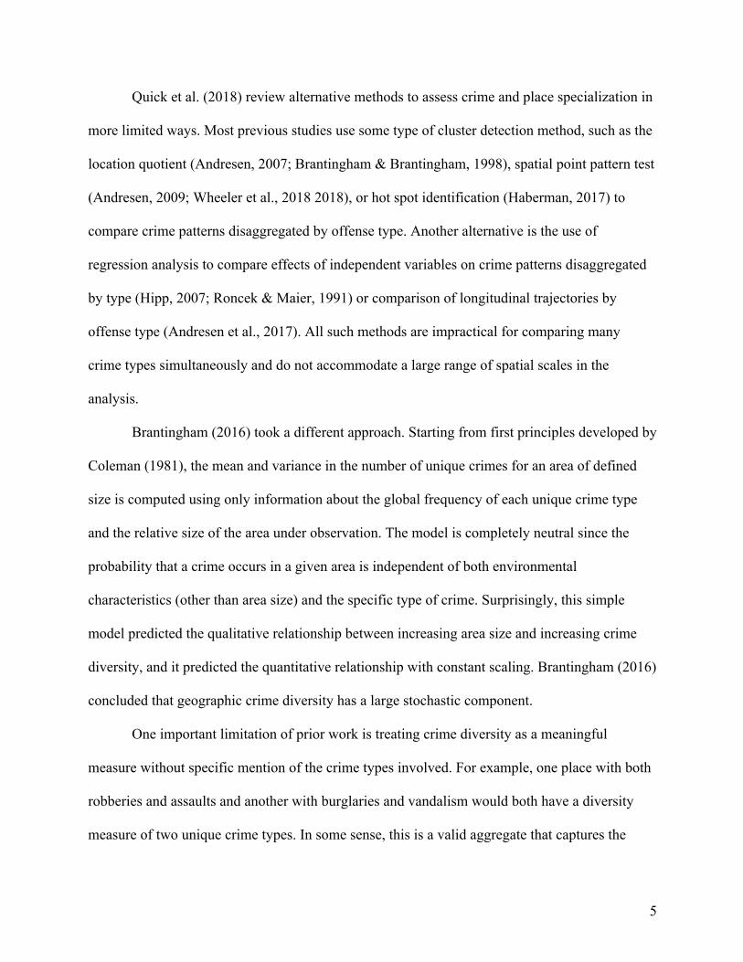
Fig. 2A shows the spatial distribution of 1,000 random selected crime incidents
overlaying a point density map of all incidents to illustrate substantial spatial clustering. Fig. 3B
shows a rank-frequency plot to describe the distribution of crimes across types. The x-axis in
Fig. 3B ranks each crime type from the most frequent (rank=1) to the least frequent crime type
(rank=S), while the y-axis is the log-frequency of each crime type. If incidents were equally
distributed across crime types, the plots would make a nearly horizontal line across the graph.
The plot in Fig. 2B, however, demonstrates that crime incidents are concentrated within types,
with just a few common crime types accounting for the majority of incidents. Thus, crimes are
concentrated both within places and within types.
[Fig. 2 about here]
We chose to aggregate crimes by randomly selecting crime locations and defining areas
of a given buffer distance around each selected location so that each place is a circular area of
fixed size. This allows us to adjust the buffer distance to create areas of any size. Arbitrary units
may be more applicable for policy and practice than standard area units such as grid cells or
census blocks because police may find it easier to target efforts at specific point locations rather
than develop responses for entire areas. We therefore find this unit of analysis defensible
theoretically and in terms of policy and practice.
To select the sample for analysis, 1000 sites are randomly selected without replacement
from the entire list of crime locations. Each place is determined by drawing a buffer distance
around each selected site for 30 area sizes ranging from micro places (0.007 square miles) to

12
large areas (6.339 square miles).4 For each sampled site, a second site of equal size is randomly
selected at least twice the buffer distance away from the first to ensure there is no spatial overlap
within pairs. The crime types occurring within the buffer distance at both sampled sites are
recorded, and this procedure is repeated for each spatial scale examined. All comparative metrics
are recorded for each sampled pair. Note that high crime areas are sampled with greater
probability than low crime areas. Whereas a spatially random sample might have been more
representative of the city landscape, our strategy samples directly from the observed crime
distribution. This is purposeful given that police often target resources toward high crime areas
to achieve the greatest overall impacts, but also includes low crime places (albeit with lower
probability). Our results are therefore more applicable to these high crime places than to low
crime places that are rarely an enforcement priority.
To summarize the observed patterns, the theoretical and empirical means and standard
deviations are computed for each spatial scale and displayed graphically in relation to area size.
The observed and theoretical values are presented in Appendix B for reference. Kolmogorov-
Smirnov D (Massey Jr, 1951) tests are used to detect differences between observed crime-area
curves and the theoretical expectations. If significant differences exist, each value of the passive
sampling model is multiplied by a constant factor such that the scaled theoretical expectation is
statistically equivalent to observed values. These scaling constants measure the difference
between the observed and theoretical values to quantify model fit. A constant equal to 1.0
indicates no scaling is used. A value between zero and 1.0 indicates that the model underpredicts
4 The area sizes used in this study are computed by increasing buffer size around sampled locations from 250 feet to 7500 feet in increments of 250. The choice of scales ensures that the range of area sizes includes micro-places that fit the original definition of Sherman et al. (1989) as areas that can be fully seen by the human eye standing at one point location (250-500 feet in either direction), as well as large intracity areas that might represent large neighborhoods or communities (6.3 square miles).

13
observed patterns, and a value greater than 1.0 indicates overprediction. Scaling by a constant
term implies that the difference between theoretical and observed values is proportional across
spatial scales, implying scale invariance of the crime-generating processes (Land et al., 1990).
The final step of analysis examines unshared crime types in greater depth to understand
how they contribute to dissimilarity between places. In this step, we want to know which offense
types are responsible for making places dissimilar. We defined two quantities. Let 𝜏/ be a count
of the number of times crime type 𝑖 is present at least once in M repeated random samples of
paired regions. For a single crime type, three random samples [present, present], [present,
absent], and [absent, present] would yield 𝜏/ = 3. Let 𝑢/ be a count of the number of times that
crime type 𝑖 is present in only one of the paired regions over M repeated samples (i.e., unshared).
In the above example, the number of times crime type i is unshared is 𝑢/ = 2. We can compare
the total frequency of a crime type 𝜏/ with the frequency that crime type is unshared to determine
whether rare or common crime types tend to be the reason that places differ in crime
composition. If common crime types are often responsible for differences in crime composition,
then identify offense-specific hot spots seems necessary from a policy/practice standpoint. If rare
crime types are implicated, then offense-specific hotspotting may not be warranted.
3 RESULTS
The first step of analysis examined total richness, shared crime types, and unshared crime
types in paired locations across spatial scales in St. Louis. Fig. 3 shows that the observed mean
values for each measure increased nonlinearly with area size. Note that the mean number of
shared crime types was much higher than the mean number of unshared types in sample pairs,
especially for larger sample area sizes (Fig. 3A). The passive sampling model matched the
14
observed patterns for both richness (D = 0.1; p > 0.05) and shared crime types (D = 0.2; p >
0.05). The observed mean number of unshared crime types is significantly higher than expected
by passive sampling (D=0.9; p<.001).
[Fig. 3 about here]
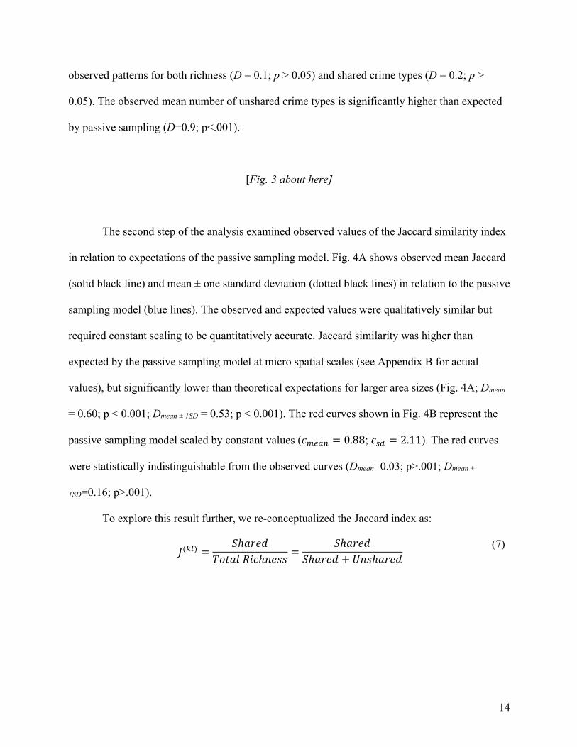
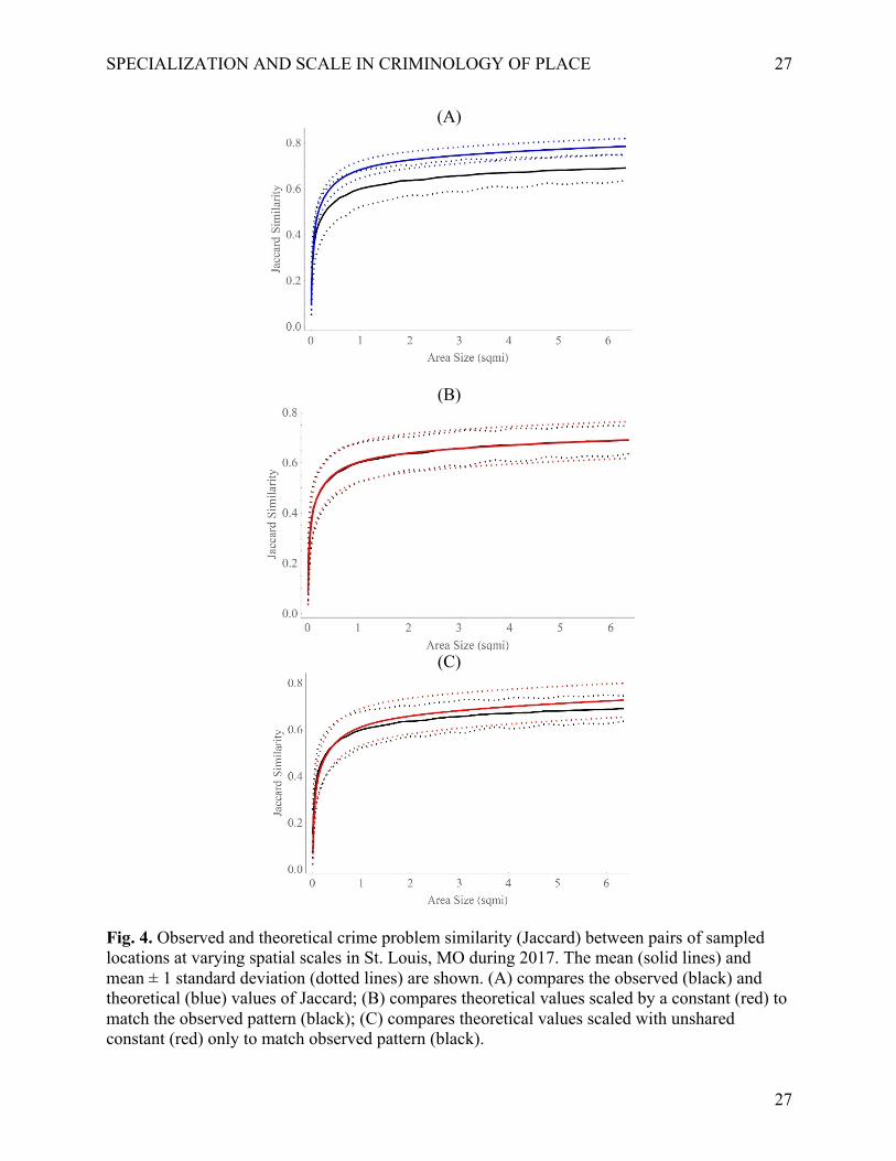
The second step of the analysis examined observed values of the Jaccard similarity index
in relation to expectations of the passive sampling model. Fig. 4A shows observed mean Jaccard
(solid black line) and mean ± one standard deviation (dotted black lines) in relation to the passive
sampling model (blue lines). The observed and expected values were qualitatively similar but
required constant scaling to be quantitatively accurate. Jaccard similarity was higher than
expected by the passive sampling model at micro spatial scales (see Appendix B for actual
values), but significantly lower than theoretical expectations for larger area sizes (Fig. 4A; Dmean
= 0.60; p < 0.001; Dmean ± 1SD = 0.53; p < 0.001). The red curves shown in Fig. 4B represent the
passive sampling model scaled by constant values (𝑐:*(1 = 0.88; 𝑐&+ = 2.11). The red curves
were statistically indistinguishable from the observed curves (Dmean=0.03; p>.001; Dmean ±
1SD=0.16; p>.001).
To explore this result further, we re-conceptualized the Jaccard index as:
𝐽("$) =
𝑆ℎ𝑎𝑟𝑒𝑑𝑇𝑜𝑡𝑎𝑙𝑅𝑖𝑐ℎ𝑛𝑒𝑠𝑠 =
𝑆ℎ𝑎𝑟𝑒𝑑𝑆ℎ𝑎𝑟𝑒𝑑 + 𝑈𝑛𝑠ℎ𝑎𝑟𝑒𝑑
(7)

15
and applied scaling to make expected mean unshared crime types match observed values. 5 The
red curves shown in Fig. 4C represent the passive sampling model when only the unshared
portion of the Jaccard index were scaled by the constant value of 𝑐;1&'()*+ = 1.37 and matched
the observed pattern (Dmean = 0.27; p > 0.05). Overall, unshared crime types drove the bulk of
proportional differences in crime problems unaccounted for by the passive sampling model.
[Fig. 4 about here]
Finally, Fig. 5 shows how the rate at which a crime is unshared depended on the rate at
which it was sampled, noting that both 𝜏/ and 𝑢/ were mediated by the size of the paired regions
under observation. Fig. 5A shows the result for small paired regions (0.007 sq mi, or a disk with
a radius of 250 feet) and Fig. 5B for large paired regions (6.339 sq mi, or a disk with a radius of
7500 feet). Starting with the larger areas shown in Fig. 5B, crime types sampled infrequently
because they were rare overall (low 𝜏/) (marked as point 1), were also infrequently the cause of
the paired regions being different (low 𝑢/). Rare crime types did not occur frequently enough to
be decisive in driving differences between locations. Crime types that were sampled at a high
rate because they are common overall (high 𝜏/) (marked as point 2) were also infrequently the
cause of paired regions being different (low 𝑢/). Common crime types were not only sampled
frequently overall, but they appear frequently in both of the paired regions under comparison on
the basis of chance. Crime types of intermediate frequency (mid quartile range between 5 and 50
5 We can rewrite the equation for Jaccard as: 𝐽(𝑘𝑙) = &('()
&('())*&('))&(()+,&('()-. We then apply the constant (c) only to
the unshared portion of the equation as follows: 𝐽(𝑘𝑙) = &('()&('())(.∗*&('))&(()+,&('()-)
.
16
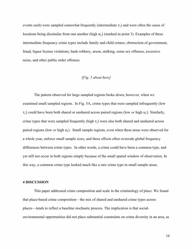
events each) were sampled somewhat frequently (intermediate 𝜏/) and were often the cause of
locations being dissimilar from one another (high 𝑢/) (marked as point 3). Examples of these
intermediate frequency crime types include family and child crimes, obstruction of government,
fraud, liquor license violations, bank robbery, arson, stalking, some sex offenses, excessive
noise, and other public order offenses.
[Fig. 5 about here]
The pattern observed for large sampled regions broke down, however, when we
examined small sampled regions. In Fig. 5A, crime types that were sampled infrequently (low
𝜏/) could have been both shared or unshared across paired regions (low or high 𝑢/). Similarly,
crime types that were sampled frequently (high 𝜏/) were also both shared and unshared across
paired regions (low or high 𝑢/). Small sample regions, even when these areas were observed for
a whole year, enforce small sample sizes, and these effects often overrode global frequency
differences between crime types. In other words, a crime could have been a common type, and
yet still not occur in both regions simply because of the small spatial window of observation. In
this way, a common crime type looked much like a rare crime type in small sample areas.
4 DISCUSSION
This paper addressed crime composition and scale in the criminology of place. We found
that place-based crime composition—the mix of shared and unshared crime types across
places—tends to reflect a baseline stochastic process. The implication is that social-
environmental opportunities did not place substantial constraints on crime diversity in an area, as

17
opportunity theories would imply (Felson & Clarke, 1998; Wilcox & Cullen, 2018; Wilcox et al.,
2003). The analyses of crime patterns in St. Louis showed that the mean total richness and mean
number of shared crime types between sampled places matches expectations from the passive
sampling model, without the need for constant scaling. This suggests that the comparative
passive sampling model, which assumes the operation of general crime cues and an absence of
individual offending specialization, is a plausible explanation for crime problem similarity
between sampled places. As it relates to policy, the findings imply that crime prevention
strategies may be better suited for identifying general crime hot spots of all offenses, rather than
identifying hot spots of specific offense types.
A caveat to the above conclusion is that sampled pairs of places often had more unshared
crime types than expected by the passive sampling model. It appeared, however, that only some
crime types really mattered for distinguishing such locations from one another. Specifically,
crime types that occurred at intermediate frequencies overall in the jurisdiction were often the
cause of places being different from one another. Importantly, these intermediate frequency
crime types were not “high profile” crimes (e.g., assault). But neither were they truly “oddball”
crimes that prompt minimal attention (Felson 2006). Crimes that occur relatively infrequently,
but were often the cause of place-based crime compositional differences (i.e., unshared crime
types), included family and child crimes, obstruction of government, fraud, liquor license
violations, bank robbery, arson, stalking, some sex offenses, excessive noise, and other public
order offenses. This observation reinforces the idea that general crime hot spot identification may
be sufficient for directing crime prevention strategies. To the extent that crime type-specific hot
spot identification is necessary, it may only need to focus on a handful of relatively uncommon
crime types.

18
The above conclusions were not invariant over spatial scale. Micro places in St. Louis
were actually more similar to one another than expected by chance alone. This is important for
the study of crime and place because micro-spatial patterns often display larger variability than
macroscopic patterns in terms of crime frequency (Mohler et al., 2018; Schnell et al., 2017;
Steenbeek & Weisburd, 2016; Weisburd, 2015). As it relates to the qualitative nature of crime
problems, we might have assumed that micro-places would be quite different from one another
in a structured way. Instead, we observed that the patterns at micro places were even more
similar than expected from the passive sampling model, which spreads crime types evenly across
place. The pattern appeared to be driven by unshared crime types. Although variation in Jaccard
similarity was larger at micro scales than at macro scales (see coefficient of variation in
Appendix B), the average dissimilarity (unshared crime types) between micro-places was lower
than expected by passive sampling. Overall, the observation was that crime problems in micro-
places were much less different from one another than is often implied.
Our study had several limitations. First, the sampling method we used does not explicitly
account for edge effects. Areas sampled from the edge of the city would not be as large in
practice as their expected sizes. We are unsure how edge effects might affect the results. Second,
the crime composition metric we used treats all dissimilar crime types as equally dissimilar
(Peet, 1974). Simple assault and aggravated assault, for example, are considered just as different
from one another as simple assault and larceny. While this may be viewed as an
oversimplification, such an assumption should also make it easier to reject the null hypothesis
that environmental crime cues are always general (i.e., no place-based specialization). If we
allowed a more nuanced classification where crime types carried a weighted dissimilarity with
other types, it would be harder to reject the null hypothesis (Lentz, 2018). Given that we find it

19
difficult to fully reject the null hypothesis, our conservative use of the crime composition metric
strengthens our conclusion that specific cues contribute much less influence than criminological
theory might expect.
The use of stochastic models, such as passive sampling, tend to be met with immediate
criticism and apprehension. One reason is because they often stand in opposition to mainstream
theoretical perspectives. In the present case, the passive sampling model challenges the claim
that variation in environmental conditions or opportunities is responsible for differences in the
types of crime that occur across places – a claim that follows directly from the tenets of
environmental criminology (Brantingham & Brantingham, 1981), opportunity theory (Wilcox &
Cullen, 2018), and the criminology of place (Weisburd et al., 2016; Weisburd et al., 2012). One
might wonder how such a model can explain an observed pattern despite a large literature
supporting the mainstream idea.
Alternatively, we may just accept that multiple types of processes (e.g., general and
specific cues, stochastic and deterministic) may be important in generating observed patterns of
interest. This idea is consistent with mechanism-based perspectives in the broader social sciences
(Hedström & Swedberg, 1998) and is making its way into the criminology of place (Bruinsma &
Pauwels, 2018; Taylor, 2015). As it pertains to this study, the passive sampling model suggests
that stochasticity dominates much of what we see in spatial patterns of crime diversity, implying
a general lack of crime and place specialization, but we acknowledge that specific cues may also
play a role in certain instances.
5 CONCLUSION

20
This paper improves on approaches for examining crime diversity across spatial scales.
Our findings contribute to a growing body of work that suggests environments have general
influence on the crime that occurs there, rather than narrowly influencing specific types of crime
events. It follows that crime prevention strategies may be better suited for identifying general
crime hot spots of all offenses, rather than identifying hot spots of specific offense types. The
comparative passive sampling model can be used to test whether places differ in the types of
crimes that occur there on the basis of chance. This approach developed herein could also be
adapted for comparing the composition of any type of place-based phenomenon. The model
leverages mathematical machinery with a long history in ecology (Chao et al., 2005; Coleman,
1981), rather than relying on simulation to generate the null distribution. The comparative
passive sampling model could complement other approaches to examining the geographic
distribution of any physical or social phenomenon across spatial scales.

21
6 REFERENCES Andresen, M. A. (2007). Location quotients, ambient populations, and the spatial analysis of
crime in Vancouver, Canada. Environment and Planning A, 39(10), 2423-2444. Andresen, M. A. (2009). Testing for similarity in area-based spatial patterns: a nonparametric
Monte Carlo approach. Applied Geography, 29(3), 333-345. Andresen, M. A., Curman, A. S., & Linning, S. J. (2017). The trajectories of crime at places:
understanding the patterns of disaggregated crime types. Journal of Quantitative Criminology, 33(3), 427-449.
Boessen, A., & Hipp, J. R. (2015). Close‐ups and the scale of ecology: Land uses and the geography of social context and crime. Criminology, 53(3), 399-426.
Braga, A. A., & Weisburd, D. (2010). Policing problem places: Crime hot spots and effective prevention. Oxford University Press on Demand.
Brantingham, P., & Brantingham, P. (1995). Criminality of place: Crime generators and crime attractors. European journal on criminal policy and research, 3(3), 5-26.
Brantingham, P. J. (2016). Crime diversity. Criminology, 54(4), 553-586. Brantingham, P. J., & Brantingham, P. L. (1981). Environmental criminology. Sage Publications
Beverly Hills, CA. Brantingham, P. J., & Brantingham, P. L. (1984). Patterns in crime. Macmillan New York. Brantingham, P. L., & Brantingham, P. J. (1998). Mapping crime for analytic purposes: location
quotients, counts, and rates. Crime mapping and crime prevention, 8, 263-288. Brantingham, P. L., & Brantingham, P. L. (1993). Environment, routine and situation: Toward a
pattern theory of crime. Advances in Criminological Theory, 5(2), 259-294. Chao, A., Chazdon, R. L., Colwell, R. K., & Shen, T. J. (2005). A new statistical approach for
assessing similarity of species composition with incidence and abundance data. Ecology letters, 8(2), 148-159.
Cloward, R. A., & Ohlin, L. E. (1960). Delinquency and opportunity: A study of delinquent gangs (Vol. 6). Routledge.
Coleman, B. D. (1981). On random placement and species-area relations. Mathematical Biosciences, 54(3-4), 191-215.
Felson, M. (2006). Crime and nature. Thousand Oaks: Sage. Felson, M., & Clarke, R. V. (1998). Opportunity makes the thief. Police research series, paper,
98. Gerell, M. (2017, June 01). Smallest is better? The spatial distribution of arson and the
modifiable areal unit problem. Journal of Quantitative Criminology, 33(2), 293-318. Ha, O. K., & Andresen, M. A. (2017). Unemployment and the specialization of criminal activity:
A neighborhood analysis. Journal of Criminal Justice, 48, 1-8. Haberman, C. P. (2017). Overlapping hot spots? Criminology & Public Policy, 16(2), 633-660. Haberman, C. P., Sorg, E. T., & Ratcliffe, J. H. (2017, September 01). Assessing the validity of
the law of crime concentration across different temporal scales. Journal of Quantitative Criminology, 33(3), 547-567.
Hipp, J. R. (2007). Income inequality, race, and place: Does the distribution of race and class within neighborhoods affect crime rates? Criminology, 45(3), 665-697.
Hipp, J. R. (2016). General theory of spatial crime patterns. Criminology, 54(4), 653-679. Hipp, J. R., & Williams, S. A. (2020). Advances in Spatial Criminology: The Spatial Scale of
Crime. Annual Review of Criminology, 3(1).

22
Hipp, J. R., Wo, J. C., & Kim, Y.-A. (2017). Studying neighborhood crime across different macro spatial scales: The case of robbery in 4 cities. Social science research, 68, 15-29.
Jaccard, P. (1908). Nouvelles recherches sur la distribution florale. Bull. Soc. Vaud. Sci. Nat., 44, 223-270.
Khorshidi, S., Carter, J., Mohler, G. et al. (2021). Explaining crime diversity with google street view. Journal of Quantitative Criminology (2021). https://doi.org/10.1007/s10940-021-09500-1.
Land, K. C., McCall, P. L., & Cohen, L. E. (1990). Structural covariates of homicide rates: Are there any invariances across time and social space? American Journal of sociology, 95(4), 922-963.
Lentz, T. S. (2018). Crime Diversity: Reexamining Crime Richness Across Spatial Scales. Journal of Contemporary Criminal Justice, 34(3), 312-335.
Massey Jr, F. J. (1951). The Kolmogorov-Smirnov test for goodness of fit. Journal of the American Statistical Association, 46(253), 68-78.
Mohler, G. O., Short, M. B., & Brantingham, P. J. (2018). The concentration dynamics tradeoff in crime hot spotting. In D. Weisburd & J. E. Eck (Eds.), Unraveling the Crime-Place Connection (Vol. 22, pp. 19-40). Routledge.
Quick, M., Li, G., & Brunton-Smith, I. (2018). Crime-general and crime-specific spatial patterns: A multivariate spatial analysis of four crime types at the small-area scale. Journal of Criminal Justice, 58, 22-32.
Real, R., & Vargas, J. M. (1996). The probabilistic basis of Jaccard's index of similarity. Systematic biology, 45(3), 380-385.
Roncek, D. W., & Maier, P. A. (1991). Bars, blocks, and crimes revisited: Linking the theory of routine activities to the empiricism of “hot spots”. Criminology, 29(4), 725-753.
Schnell, C., Braga, A. A., & Piza, E. L. (2017). The influence of community areas, neighborhood clusters, and street segments on the spatial variability of violent crime in Chicago. Journal of Quantitative Criminology, 33(3), 469-496.
Schreck, C. J., McGloin, J. M., & Kirk, D. S. (2009). On the origins of the violent neighborhood: A study of the nature and predictors of crime‐type differentiation across Chicago neighborhoods. Justice Quarterly, 26(4), 771-794.
Spelman, W., & Eck, J. E. (1987). Problem-oriented policing. US Department of Justice, National Institute of Justice.
Steenbeek, W., & Weisburd, D. (2016). Where the action is in crime? An examination of variability of crime across different spatial units in The Hague, 2001–2009. Journal of Quantitative Criminology, 32(3), 449-469.
Taylor, R. B. (2015). Community criminology: Fundamentals of spatial and temporal scaling, ecological indicators, and selectivity bias. NYU Press.
Weisburd, D. (2015). The law of crime concentration and the criminology of place. Criminology, 53(2), 133-157.
Weisburd, D., Maher, L., Sherman, L., Buerger, M., Cohn, E., & Petrisino, A. (1992). Contrasting crime general and crime specific theory: The case of hot spots of crime. Advances in Criminological Theory, 4(1), 45-69.
Wheeler, A. P., Steenbeek, W., & Andresen, M. A. (2018). Testing for similarity in area‐based spatial patterns: Alternative methods to Andresen's spatial point pattern test. Transactions in GIS, 22(3), 760-774.

23
Wilcox, P., & Cullen, F. T. (2018). Situational Opportunity Theories of Crime. Annual Review of Criminology, 1(1), 123-148.
Wilcox, P., Land, K. C., & Hunt, S. A. (2003). Criminal circumstance: A dynamic multi-contextual criminal opportunity theory. Transaction Publishers.

24
Fig. 1. Graphical representation comparing crime composition between two hypothetical places k and l. Each dot represents a unique crime type and the shaded portion of the Venn diagram indicates which crime types are counted in the metric. (A) shows the number of unique crime types occurring in place k; (B) shows the number of unique crime types occurring in place l; (C) shows the number of shared crime types occurring in both places; (D) shows the number of unshared crime types occurring in either place k or l, but not both. The total richness of both places is the sum of the number of shared and unshared crime types or equivalently the sum of crime types in places k and l minus the number shared (total richness=8). Jaccard similarity is the proportion of the total number of unique crime types shared by both places (𝐽"$ = <
== 0.375).
Adapted from Chao et al. (2005).

Unpublished Working Paper October 16, 2021
(A)
(B)
Fig. 2. Concentration of crime across space and crime type in St. Louis, 2017. (A) Random sample of 1,000 crimes overlaying kernel density map of all crimes. (B) Rank-frequency plot showing the distribution of incidents across crime types St. Louis (black plots; S = 161 unique crime types). The y-axis is sorted from the most frequent crime type (rank=1) to the least frequent, and the x-axis shows the log-frequency of each type. Crime types that occur only once in the data have log-frequency equal to zero.
0 50 100 1500
2
4
6
8
Rank
LogFrequency
Downtown
Forest Park

SPECIALIZATION AND SCALE IN CRIMINOLOGY OF PLACE 26
26
(A)
(B)
Fig. 3. Observed and theoretical mean values of crime richness (black), shared crime types (blue), and unshared crime types (red) in pairs of sampled locations as a function of area size in St. Louis, MO during 2017. (A) shows observed patterns only and (B) compares observed patterns (solid lines) and theoretical expectations (dashed lines). Theoretical expectations represent passive sampling model.
SPECIALIZATION AND SCALE IN CRIMINOLOGY OF PLACE 27
27
(A)
(B)
(C)
Fig. 4. Observed and theoretical crime problem similarity (Jaccard) between pairs of sampled locations at varying spatial scales in St. Louis, MO during 2017. The mean (solid lines) and mean ± 1 standard deviation (dotted lines) are shown. (A) compares the observed (black) and theoretical (blue) values of Jaccard; (B) compares theoretical values scaled by a constant (red) to match the observed pattern (black); (C) compares theoretical values scaled with unshared constant (red) only to match observed pattern (black).

SPECIALIZATION AND SCALE IN CRIMINOLOGY OF PLACE 28
28
(A)
(B)
Fig. 5. Relationship between observed total frequency and sample unshared frequency in sample pairs for each unique crime type (N = 161 Types) in St. Louis, MO 2017. (A) shows relationship for 0.007 square mile areas; (B) shows relationship for 6.338 square mile areas. Crime types that occur only once have log frequency equal to zero.
1 2
3