Modeling and Design of Buoyancy Driven Equipment for Deep

Modeling and Design of Buoyancy Driven Equipment for Deep OceanSensing

Sam Fladung1, James Truman2 and Anthony Westphal3

Abstract— This paper presents a view of modeling anddesigning buoyancy driven systems for deep ocean research.Buoyancy engines provide a method to move systems verticallywithin the water column and maintain depth with minimal en-ergy. A simple dynamics simulator is presented to simulate thesystem and characterize its robustness to parameter variations.A test fixture and methodology is shown for characterizinghydraulic pump performance over the range of pressures andrates required for the buoyancy system.

I. INTRODUCTION

A. Examples of buoyancy driven systems

There are many example of buoyancy driven systems incurrent operation. These include the APEX (AutonomousProfiling Explorer) profiling floats. These are buoyancydriven drifting sensor systems. They are capable of au-tonomous missions exceeding four years in length to depthsof 2000m. The floats carry a variety of sensors and are usedin applications ranging from ocean modeling to biogeochem-ical analysis. These are built around a cylindrical (eitheraluminum or carbon fiber) hull (Figure 1).

The APEX Deep extends this capability to 6000m of depthand can run more than 150 autonomous vertical profiles.They are built using a buoyancy engine housed within a glasssphere (Figure 2).

The Slocum Glider uses a buoyancy engine in addition toa variable pitch mechanism and rudder to allow the vehicleto navigate through the ocean. These gliders are capable ofautonomous deployments of up to 18 months and can workat depths of up to 1000m (Figure 3). Systems are availableusing alkaline, lithium primary and rechargeable lithium ionbatteries. A 3500m version is currently in development.These systems have crossed oceans as part of the Rutger’sChallenger Program.[1]

II. SIMPLE DYNAMICS SIMULATOR

A simplified view of the vehicle dynamics can look atjust the vertical component (ie an APEX float or standalonebuoyancy engine). The free response of the system can berepresented as a two variable state system. The two statevariables are depth (x) and speed of change of depth (x).

1Sam Fladung is an Electrical Engineer at Teledyne WebbResearch, 49 Edgerton Dr, North Falmouth, MA [email protected]

2James Truman is a Hardware Engineering Manager at Teledyne WebbResearch, 49 Edgerton Dr, North Falmouth, MA 02556

3Anthony Westphal is a Mechanical Engineer at Teledyne Benthos, 49Edgerton Dr, North Falmouth, MA 02556

Fig. 1. Teledyne APEX Profiling Float

Fig. 2. Teledyne APEX Deep Profiling Float

Fig. 3. Teledyne Slocum Glider

These can be represented by a vector (X).

X =

[xx

](1)

The dynamics of the system are shown in (2) (where m =system mass and

∑F is the sum of all forces acting on the

system:

x =

∑F

m(2)

The forces acting on the system include:• Gravity (weight)• Buoyancy• DragThe gravity force is calculated in (3).

Fg = m ∗ g (3)

The equation for the magnitude of the drag force is shownin (4) with Cd as the drag coefficient and A as the cross-sectional area.

||Fd|| =1

2∗ ρCd ∗A ∗ x2 (4)

Note that this force must always oppose the direction oftravel. Equation (5) shows the drag equation with the correctsign.

Fd = −1

2∗ ρCd ∗A ∗ x2 ∗ sgn(x) (5)

The buoyancy force is dependent on the volume of the systemand the density of water at that depth/temperature. Thesystem will compress due to both pressure and temperature.The pressure component is defined in (6) where the constantα represents the compressibility of the system in responseto pressure.

dV

V= −α∆P (6)

The temperature component is defined in (7) where theconstant β represents the change of volume in response to atemperature change.

dV

V= β∆T (7)

These two are coupled together, although ignoring the cou-pling does not introduce significant error over the normaloperating conditions. This removes a quadratic term andsimplifies the simulation.

Equation (8) shows the combined ∆V equation.

dV

V= β∆T − α∆P (8)

The density of seawater is depth, temperature and salinitydependent. The density can be calculated using the UNESCOequation of state [3].

The buoyancy force calculation is shown in (9) and (10).

FB = Vsys ∗ ρH2O ∗ g (9)

Parameter ValuePressure Compressibility (α) 3e-6 1

dBarThermal Compressibility (β) 2e-5 1

KSystem Volume (V) 0.1080 m3

System Mass (m) 113.5 kgArea 0.0706 m3

Drag Coefficient (Cd) 1.5

FB = Vinit ∗ (1− α∆P ) ∗ (1 + β∆T ) ∗ ρH2O ∗ g (10)

The system may be simulated in the discrete time domainusing the formula shown in (11) and (12)

xn = xn−1 + dt ∗ x (11)

xn = xn−1 + dt ∗ x (12)

This method assumes that dt is small relative to thesystem response. To use larger values of dt, more accurateapproximations can be used to interpolate (Trapezoidal orsolving the ODE in between each set of points for example(eg. using the Runge-Kutta algorithm)).

III. EXAMPLE UNCONTROLLED SIMULATIONS

Given the equations in section II it is possible to simulatethe descent of the system through the water column.

Figure 4 shows the simulated trajectory for a system withthe properties shown in Table III.

0 2 4 6 8 10 12

Time (hrs)

0

500

1000

1500

2000

2500

3000

3500

Dep

th (

m)

Depth vs Time

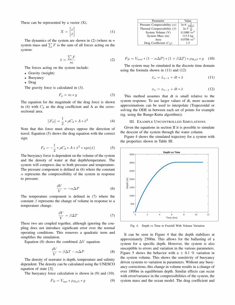
Fig. 4. Depth vs Time in Freefall With Volume Variation

It can be seen in Figure 4 that the depth stabilizes atapproximately 2500m. This allows for the ballasting of asystem for a specific depth. However, the system is alsosusceptible to errors and variation in the various parameters.Figure 5 shows the behavior with a ± 0.1 % variation inthe system volume. This shows the sensitivity of buoyancydriven systems to variation in parameters. Without any buoy-ancy corrections, this change in volume results in a change ofover 1800m in equilibrium depth. Similar effects can occurwith error/variance in the compressibilities of the system, thesystem mass and the ocean model. The drag coefficient and

system area will change how long the system takes to reachsteady state, but will not change the final depth achieved.

0 2 4 6 8 10 12

Time (hrs)

0

500

1000

1500

2000

2500

3000

3500

4000

Dep

th (

m)

Depth vs Time

Vap:0.107892Vap:0.108Vap:0.108108

Fig. 5. Depth vs Time in Freefall

IV. COMPRESSIBILITY AND STABILITY

An interesting property of these buoyancy driven systemsis that as long as the system is less compressible than theseawater, it will be stable in the water column (neglectinginternal waves or other water density boundaries). This canbe seen from the fact that as the depth is increased, thechange in the density of the system will be less than thechange on the water density (based on stiffness property).This will result in an upwards buoyancy force returning thesystem towards its equilibrium point. Likewise, if the systemis disturbed upwards, the density of the system will decreaseslower than the water, giving it a downwards force to returntoward its equilibrium position. This means that energy isnot required for vertical adjustments to maintain the depthonce equilibrium is reached.

The downside of this stability is that the greater thecompressibility difference between the water and the system,the more buoyancy volume must be used to move the systemby a fixed amount vertically in the water column.

V. CONTROLLING THE BUOYANCY

The buoyancy of the system can be controlled by changingthe systems volume. If the volume increases while the massremains constant, the system will move upwards in thewater column. This change in buoyancy can be achieved bypumping oil from inside the system into an external bladder.The size of the bladder and internal oil reservoir capacitywill limit the amount of buoyancy that can be achieved bya given system.

To simulate this buoyancy control, a simple controller isimplemented. The purpose of this controller is to show thatthe system can be controlled over the parameter variationand need not be representative of the final control algorithm.

TABLE ICONTROLLER PARAMETERS

Parameter Value

PD Control P term 0.00001m2

sPD Control D term 0.01m2

Total Oil Volume 0.0040 m3

Oil Flow Rate Limit Out 2.5e-5 m3/sOil Flow Rate Limit In 6.3e-6 m3/s

Target Depth 2500m

TABLE IISYSTEM PARAMETER VARIATION

Parameter VariationVolume ±0.5%

Pressure Compressibility (α) ±20%Coefficient of Thermal Expansion (β) ±20%

Drag Coefficient (Cd) ±50%

The controller outputs the desired oil volume rate of change(m3/s) as shown in (13)

dV

dt= pterm ∗ (x− xtarget) + dterm ∗ x (13)

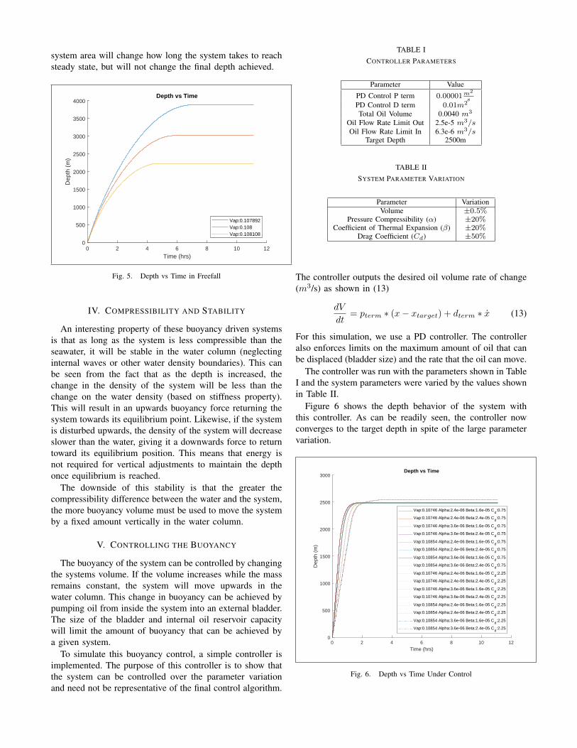
For this simulation, we use a PD controller. The controlleralso enforces limits on the maximum amount of oil that canbe displaced (bladder size) and the rate that the oil can move.

The controller was run with the parameters shown in TableI and the system parameters were varied by the values shownin Table II.

Figure 6 shows the depth behavior of the system withthis controller. As can be readily seen, the controller nowconverges to the target depth in spite of the large parametervariation.

0 2 4 6 8 10 12

Time (hrs)

0

500

1000

1500

2000

2500

3000

Dep

th (

m)

Depth vs Time

Vap:0.10746 Alpha:2.4e-06 Beta:1.6e-05 Cd:0.75
















Fig. 6. Depth vs Time Under Control

VI. BUOYANCY CONTROL ENERGY REQUIREMENTS

The energy requirements for a buoyancy system are de-pendent on the amount of oil flow and the depth at whichit is pumped. Equation (14) shows that hydraulic work isthe product of the volume of fluid moved and the pressureagainst which it is moved.

W = p ∗ V (14)

For a stable system (less compressible than the seawater),the energy is only needed to stop the descent or change depth.The control algorithm chosen can tradeoff energy use forsystem descent speed. Essentially, the earlier oil is pumpedout to slow the system, the less energy it uses, but the longerit takes to reach the target depth.

A worst case energy usage can be estimated by assumingthat the entire volume is pumped at the target depth. In thiscase, the hydraulic work required is defined in (15).

Wmax = ptarget ∗ Vbladder (15)

In addition, there will be losses in the system. See sectionVII for examples of the pump efficiencies.

If the controller is modelled, the simulation can give anenergy use estimate. Figure 7 shows the energy used withthe simple simulation controller. The energy is around halfthe worst case energy.

Energy Use of Buoyancy System

0 1 2 3 4 5 6

Energy Used (J) 104

V:0.107 :2.4e-06 :1.6e-05 Cd:0.75

V:0.107 :2.4e-06 :2.4e-05 Cd:0.75

V:0.107 :3.6e-06 :1.6e-05 Cd:0.75

V:0.107 :3.6e-06 :2.4e-05 Cd:0.75

V:0.109 :2.4e-06 :1.6e-05 Cd:0.75

V:0.109 :2.4e-06 :2.4e-05 Cd:0.75

V:0.109 :3.6e-06 :1.6e-05 Cd:0.75

V:0.109 :3.6e-06 :2.4e-05 Cd:0.75

V:0.107 :2.4e-06 :1.6e-05 Cd:2.25

V:0.107 :2.4e-06 :2.4e-05 Cd:2.25

V:0.107 :3.6e-06 :1.6e-05 Cd:2.25

V:0.107 :3.6e-06 :2.4e-05 Cd:2.25

V:0.109 :2.4e-06 :1.6e-05 Cd:2.25

V:0.109 :2.4e-06 :2.4e-05 Cd:2.25

V:0.109 :3.6e-06 :1.6e-05 Cd:2.25

V:0.109 :3.6e-06 :2.4e-05 Cd:2.25

Fig. 7. Energy Used To Stabilize At Depth

VII. BUOYANCY PUMP CHARECTERIZATIONS

The pump chosen for a buoyancy system is primarilyselected for pressure, pump rate, and efficiency. The pumpmust be able to pump against at least the ocean pressureat the maximum expected depth plus a safety factor. Thepump rate determines how fast the system can change itsbuoyancy. A faster rate allows the system to move quickerbetween different depths. Efficiency determines the energyrequirements for the system. In addition, there are oftenmechanical and electrical constraints on the size and powerof the system.

A. Pump Test Setup

In order to evaluate hydraulic pumps for their suitabilityin specific buoyancy applications, the following test setupshown in Figure 8 was used. The fixture connects the pumpbetween two reservoirs. The hydraulic flow is routed throughan adjustable pressure relief valve to simulate the oceanpressure. The mass of the oil moved through the system ismeasured by a scale under the output reservoir. In order toavoid startup transient effects, the pump is brought to fullspeed several seconds prior to the measurements beginning.This alleviates accelleration effects. The pump and inputreservoir are held in a thermal chamber at approximately4°C as this is the expected operating range.

Input

Reservoir

Output

Reservoir

Motor Pump

Adjustable Relief Valve

Scale

Pressure

Sensor

Power Supply

Power Supply

Power Supply

Power Supply

Ammeter

Ammeter

Ammeter

Ammeter

Motor Controller Motor

Volt Meter

Thermocouple

Throttle

Jeti Translator

Fig. 8. Test Fixture Block Diagram for Pump Testing. Shows the hydraulicand electrical connections of the system.

To evaluate the pump the pump motor speed and reliefvalve pressure are used as control variables. The motor speed,output pressure, input current, input voltage and reservoirmass are measured and recorded while the system is runningat steady state. Startup and stop transients are removed fromthe data.

B. Pump System Under Test

An example pump with measurements is included here.The pump in this example was a radial piston pump with anominal displacement of 0.63 cc/rev.

C. Visualizing Pump Data

The system efficiency, effective displacement and powerusage are calculated for each test using (16) to (20). Theelectrical power is calculate as

Pin = mean(Iin ∗ Vin) (16)

where Pin is the electrical power input, Iin represents themeasured current inputs and Vin represents the measuredvoltage inputs to the motor system.

The electrical energy used is calculated as

Uin = Pin ∗∆t (17)

where Uin is the energy used and ∆t is the test time interval.The hydraulic output work is calaculated as

Wout = mean(p) ∗ ∆m

ρfluid(18)

where Wout is the output work, p is the measured pressuresignal, ∆m is the change in mass over the test time intervaland ρfluid is the density of the fluid at the test temperature.

The efficiency (η) is calculated in (19)

η =Wout

Uin(19)

The effective displacement is calculate as

Qv =∆m

ρfluid ∗∆t

1

ωmotor(20)

where Qv is the effective displacement, and ωmotor is theangular speed of the motor.

These are plotted on a contour plot with intermediatevalues interpolated on a grid between them. This shows theexpected value between actual measurements. Parts of thegraph region are outside of the test region either due toexceeding the power requirements of the test setup or beingbelow the expected operating speed of the motor. These areasappear as white in the graphs. The actual data points areoverlayed on the plots as red circles to indicate the locationsof measurements. Plots are shown with actual measurementsfor an example motor/pump combination.

Figure 9 shows the electrical power required to run thepump at the operating point (speed and pressure). The powerrequirement drives other system considerations includingbattery sizing. Depending on the application, this may limitthe speed at which the pump can be run at different depths.The equipotential lines on the contour plots show the safeoperating limits for a given power limitation.

Fig. 9. Power vs RPM and Pressure For Hydraulic Pump

The mechanical efficiency plot in Figure 10 shows wherethe pump operates most efficiently. Unfortunately the optimalpoint for efficiency may lie outside of the safe operating areafrom a power or current perspective and so a compromisemust be reached. The maximum efficiency for this pump andmotor combination was shown to be around 4000dBar.

Fig. 10. Mechanical Efficiency vs RPM and Pressure For Hydraulic Pump

The final results plot is shown in Figure 11 which showsthe effective displacement of the pump. This shows howmuch oil is moved with each rotation of the pump. This canbe used to identify mismatches of oil viscosity to the pump.If there is an excessive drop in the effective displacement,the oil may have insufficient viscosity for use at the testedtemperature.

Fig. 11. Volumetric Efficiency vs RPM and Pressure For Hydraulic Pump

D. Viscosity

The hydraulic fluid used with the pump is an integral partof the system. The viscosity of the oil can have a largeeffect on pump performance. If the viscosity is too low,

the volumetric efficiency is reduced. If it is too high, thefrictional losses in the system will become large [2]. Theviscosity is a temperature-dependent parameter. This meansit is important to test the system under the temperature rangeunder which it will be operated.

VIII. CONCLUSIONS

Buoyancy engines can be used to move equipment todesired depths in the ocean. They provide the ability to adjustfor parameter variation of the system. When made stifferthan the water, they require negligible energy to maintain adepth. Pumps can be sized to deliver the required buoyancyfor a system and tested to verify their behavior over theoperating range. Simulation and the test setup provide aneffective design tool for optimizing performance.

REFERENCES

[1] Dobson, Collin, J. Mart, N. Strandskov, J. Kohut, O. Schofield, S.Glenn, C. Jones, C. Barrera. 2013. The Challenger Glider Mission: AGlobal Ocean Predictive Skill Experiement, Proceedings Oceans IEEEMTS 2013, San Diego.

[2] Rydberg, Karl-Erik. (2013). Hydraulic Fluid Properties and theirImpact on Energy Efficiency. 447-453. 10.3384/ecp1392a44.

[3] UNESCO (1981) Tenth report of the joint panel on oceanographictables and standards. UNESCO Technical Papers in Marine Science,Paris, 25 p

Documents

Modeling and Design of Buoyancy Driven Equipment for Deep