Embed Size (px)
Citation preview

Modeling and Controller Design of a Wind
Energy Conversion System Including a
Matrix Converter
by
S. Masoud Barakati
A thesis
presented to the University of Waterloo
in fulfillment of the
thesis requirement for the degree of
Doctor of Philosophy
in
Electrical and Computer Engineering
Waterloo, Ontario, Canada, 2008
© S. Masoud Barakati 2008

ii
AUTHOR'S DECLARATION
I hereby declare that I am the sole author of this thesis. This is a true copy of the thesis, including any
required final revisions, as accepted by my examiners.
I understand that my thesis may be made electronically available to the public.

iii
Abstract
In this thesis, a grid-connected wind-energy converter system including a matrix converter is
proposed. The matrix converter, as a power electronic converter, is used to interface the induction
generator with the grid and control the wind turbine shaft speed. At a given wind velocity, the
mechanical power available from a wind turbine is a function of its shaft speed. Through the matrix
converter, the terminal voltage and frequency of the induction generator is controlled, based on a
constant V/f strategy, to adjust the turbine shaft speed and accordingly, control the active power
injected into the grid to track maximum power for all wind velocities. The power factor at the
interface with the grid is also controlled by the matrix converter to either ensure purely active power
injection into the grid for optimal utilization of the installed wind turbine capacity or assist in
regulation of voltage at the point of connection. Furthermore, the reactive power requirements of the
induction generator are satisfied by the matrix converter to avoid use of self-excitation capacitors.
The thesis addresses two dynamic models: a comprehensive dynamic model for a matrix converter
and an overall dynamical model for the proposed wind turbine system.
The developed matrix converter dynamic model is valid for both steady-state and transient
analyses, and includes all required functions, i.e., control of the output voltage, output frequency, and
input displacement power factor. The model is in the qdo reference frame for the matrix converter
input and output voltage and current fundamental components. The validity of this model is
confirmed by comparing the results obtained from the developed model and a simplified
fundamental-frequency equivalent circuit-based model.
In developing the overall dynamic model of the proposed wind turbine system, individual models
of the mechanical aerodynamic conversion, drive train, matrix converter, and squirrel-cage induction
generator are developed and combined to enable steady-state and transient simulations of the overall
system. In addition, the constraint constant V/f strategy is included in the final dynamic model. The
model is intended to be useful for controller design purposes.
The dynamic behavior of the model is investigated by simulating the response of the overall model
to step changes in selected input variables. Moreover, a linearized model of the system is developed
at a typical operating point, and stability, controllability, and observability of the system are
investigated.

iv
Two control design methods are adopted for the design of the closed-loop controller: a state-
feedback controller and an output feedback controller. The state-feedback controller is designed based
on the Linear Quadratic method. An observer block is used to estimate the states in the state-feedback
controller. Two other controllers based on transfer-function techniques and output feedback are
developed for the wind turbine system.
Finally, a maximum power point tracking method, referred to as mechanical speed-sensorless
power signal feedback, is developed for the wind turbine system under study to control the matrix
converter control variables in order to capture the maximum wind energy without measuring the wind
velocity or the turbine shaft speed.

v
Acknowledgements
I would like to express my deepest gratitude to my supervisors, Professor Mehrdad Kazerani and
Professor J. Dwight Aplevich for their generous support and supervision, and for the valuable
knowledge that they shared with me. I learned valuable lessons from their personality and their
visions.
I am also grateful to my Doctoral Committee Members, Professor Daniel E. Davison, Professor
Claudio A. Canizares, and Professor Amir Khajepour and also the external examiner, Professor M.
Reza Iravani.
With great thanks, I want to acknowledge the partial financial support of the Iranian Ministry of
Science, Research, and Technology and the Natural Sciences and Engineering Research Council
(NSERC) of Canada.
My thanks are also extended to the ECE Department of the University of Waterloo for a nice
atmosphere, kind treatment and support.
Special thanks to my friends, Dr. X. Chen, Naghmeh Mansouri and Fariborz Rahimi for their
helpful discussion and valuable comments, and also thanks to Mrs Jane Russwurm for proofreading.
My grate thanks to my parents, brothers and sister for their unconditional love and their support
during the long years of my studies.
Finally, and most importantly, I would like to express my deep appreciation to my beloved wife,
Mehri, for all her encouragement, understanding, support, patience, and true love throughout the ups
and downs.
As always, I thank and praise God by my side.

vi
Dedication
This thesis is dedicated to my mother, my wife, Mehri, and my lovely angel, Samin.

vii
Table of Contents AUTHOR'S DECLARATION ...............................................................................................................ii Abstract .................................................................................................................................................iii Acknowledgements ................................................................................................................................ v Dedication .............................................................................................................................................vi Table of Contents .................................................................................................................................vii List of Figures .......................................................................................................................................xi List of Tables.......................................................................................................................................xvi List of Symbols ..................................................................................................................................xvii Acronyms ........................................................................................................................................... xxv Chapter 1 Introduction............................................................................................................................ 1
1.1 Research Motivation..................................................................................................................... 1 1.1.1 Growth of Installed Wind Turbine Power ............................................................................. 1 1.1.2 Environmental Advantages of Wind Energy......................................................................... 2
1.2 Historical Background and Literature Survey .............................................................................. 2 1.3 Wind Energy Conversion System (WECS).................................................................................. 4
1.3.1 Classification of Wind Turbine Rotors.................................................................................. 5 1.3.2 Common Generator Types in Wind Turbines ....................................................................... 7 1.3.3 Mechanical Gearbox.............................................................................................................. 9 1.3.4 Control Method ..................................................................................................................... 9 1.3.5 Power Electronic Converter ................................................................................................ 11 1.3.6 Different Configurations for Connecting Wind Turbines to the Grid ................................. 15 1.3.7 Starting and disconnecting from electrical grid................................................................... 18
1.4 Literature Survey on Using Matrix Converters in Wind Turbine Systems ................................ 19 1.5 Thesis Objectives ....................................................................................................................... 20 1.6 The Proposed Wind Energy Conversion System ....................................................................... 21 1.7 Thesis Outline............................................................................................................................. 22
Chapter 2 Matrix Converter Structure and Dynamic Model ................................................................ 23 2.1 Introduction ................................................................................................................................ 23 2.2 Static Frequency Changer (AC/AC Converter).......................................................................... 24 2.3 Matrix Converter Structure......................................................................................................... 25 2.4 Modulation Strategy for the Matrix Converter........................................................................... 27

viii
2.5 Commutation Problems in Matrix Converter............................................................................. 30 2.6 Simulation Results of the Matrix Converter Based on SVPWM............................................... 31 2.7 An Overall Dynamic Model for a the Matrix Converter System............................................... 34
2.7.1 Low- Frequency Transformation Matrix ............................................................................ 34 2.7.2 Output voltage and input current of Matrix Converter ....................................................... 35 2.7.3 Matrix Converter Equivalent Circuit Model ....................................................................... 37 2.7.4 Evaluation of Matrix Converter Equivalent Circuit Model ................................................ 37
2.8 Matrix Converter State-Space Dynamic Model......................................................................... 41 2.8.1 Matrix Converter Equations Referred to One-Side............................................................. 41 2.8.2 Voltage Equations at Input Side of Matrix Converter Circuit ............................................ 42 2.8.3 Voltage Equations at the Output Side of Matrix Converter Circuit .................................... 42 2.8.4 Current Equations ............................................................................................................... 43 2.8.5 Matrix converter Equations in qdo Reference Frame ......................................................... 44 2.8.6 State-Space-qdo Model of the Matrix Converter System ................................................... 47 2.8.7 Power Formula in the State-Space-qdo Model ................................................................... 52
2.9 Evaluation of the Matrix Converter Dynamic Model ................................................................ 55 2.10 Summary .................................................................................................................................. 59
Chapter 3 Overall Dynamic Model of the Wind Turbine System and Small Signal Analysis ............ 60 3.1 Introduction................................................................................................................................ 60 3.2 Dynamic Model of the Wind Turbine System ........................................................................... 61
3.2.1 Aerodynamic Model ........................................................................................................... 62 3.2.2 Mechanical Model .............................................................................................................. 65 3.2.3 Induction Machine Model................................................................................................... 67 3.2.4 Gearbox Model ................................................................................................................... 71 3.2.5 Grid model .......................................................................................................................... 72 3.2.6 Wind Speed Model ............................................................................................................. 72
3.3 Overall Dynamic Model of the Wind Turbine System .............................................................. 76 3.4 Verification of the Overall Dynamic Model .............................................................................. 79
3.4.1 Starting the Wind Turbine System...................................................................................... 79 3.4.2 Steady-State Performance of the System ............................................................................ 81 3.4.3 Step Response of the System .............................................................................................. 84
3.5 Overall Dynamic Model and Constant V/f Strategy .................................................................. 87

ix
3.5.1 Verification of the Overall Dynamic Model with Constant V/f Strategy ............................ 88 3.6 Limitations of the variables changes .......................................................................................... 90 3.7 Linearized Model of the Wind Turbine System ......................................................................... 91 3.8 Linearized Model Performance Evaluation................................................................................ 93 3.9 Local Stability Evaluation .......................................................................................................... 95 3.10 Controllability and Observability ............................................................................................. 96
3.10.1 Gramian method ................................................................................................................ 96 3.11 Balanced Realization ................................................................................................................ 97 3.12 Reduced-Order Model .............................................................................................................. 99 3.13 Summary ................................................................................................................................ 101
Chapter 4 Controller Design for the Wind Turbine System under Study........................................... 103 4.1 Introduction .............................................................................................................................. 103 4.2 Augmented System with Integrator.......................................................................................... 104
4.2.1 Closed-loop state-space equations..................................................................................... 105 4.3 LQ method for State-Feedback Controller Design................................................................... 106
4.3.1 Design of an LQ Controller for the Wind Turbine System ............................................... 107 4.3.2 Evaluation of the Closed-loop System with LQ Controller............................................... 108
4.4 Eigenvalue Placement of an LQ Optimal System .................................................................... 110 4.4.1 Boundary of the LQ optimal Closed-Loop Eigenvalues ................................................... 111 4.4.2 Eigenvalue Placement Using a Genetic Algorithm Approach .......................................... 112 4.4.3 Applying GA to LQ Optimal Controller for the Wind Turbine System............................ 114
4.5 Observer-based State-Feedback Controller with integral Control............................................ 119 4.5.1 Design of an Optimal Observer for the Wind Turbine System ......................................... 119
4.6 Design of a Controller Using Transfer Function Techniques................................................... 124 4.6.1 Design of a Decoupling Controller.................................................................................... 124 4.6.2 Reducing cross-channel interactions ................................................................................. 125 4.6.3 Applying the reduced cross-channel interactions approach to the wind turbine system ... 126 4.6.4 Sequential Loop Closure Approach (SLC)........................................................................ 131 4.6.5 Applying the SLC approach to the wind turbine system................................................... 132 4.6.6 Closed-Loop Wind Turbine Nonlinear Model with the SLC Controller........................... 140
4.7 Summary .................................................................................................................................. 143 Chapter 5 Maximum Power Point Tracking Control for the Proposed Wind Turbine System.......... 145

x
5.1 Introduction.............................................................................................................................. 145 5.2 Maximum Power Tracking Concept ........................................................................................ 146 5.3 Maximum Power Point Tracking Methods .............................................................................. 147
5.3.1 Perturbation and Observation Method .............................................................................. 147 5.3.2 Wind Speed Measurement Method................................................................................... 148 5.3.3 Power Signal Feedback (PSF) Control ............................................................................. 149 5.3.4 Mechanical Speed-Sensorless PSF method ...................................................................... 151
5.4 Implementing the P&O Method for a Small Wind Turbine System including a Matrix
Converter........................................................................................................................................ 157 5.5 Implementing the Mechanical Speed-Sensorless PSF Method on the Wind Turbine System
under Study .................................................................................................................................... 159 5.5.1 Evaluation of the Mechanical Speed-sensorless PSF method with the instantaneous wind
velocity....................................................................................................................................... 165 5.6 Summary .................................................................................................................................. 166
Chapter 6 Conclusions ....................................................................................................................... 167 6.1 Summary and conclusions ....................................................................................................... 167 6.2 Contributions............................................................................................................................ 170 6.3 Suggestions for Future work .................................................................................................... 171
Appendix A Practical Bidirectional Switch Configuration for the Matrix Converter ....................... 173 Appendix B Switch State Combinations in MC ................................................................................ 175 Appendix C Modulation Algorithm and SVPWM ............................................................................ 177 Appendix D A Comparison Between PWM and SVPWM Techniques ............................................ 189 Appendix E Safe Commutation in MC and Indirect MC Topology .................................................. 193 Appendix F Calculating the term (K0D)DT(K0)-1................................................................................ 200 Appendix G Overall Dynamic Model Equations of the Wind Turbine System................................. 205 Appendix H Incorporating Constant V/f strategy in the Overall Dynamic Model Equations............ 211 Appendix I Linearized Model Of the Wind Turbine System............................................................. 215 Appendix J Luenberger Observer Construction................................................................................. 219 Appendix K Transfer Function of the Wind Turbine System............................................................ 223 Appendix L Parameters of the system under study............................................................................ 224 Bibliography………………………………………………………………………………………...225

xi
List of Figures Fig. 1-1: Installed wind turbine power worldwide and in Canada [1][2] ............................................... 2 Fig. 1-2: Block diagram of a WECS ...................................................................................................... 4 Fig. 1-3: (a) a typical vertical-axis turbine (the Darrius rotor) (b) a horizontal-axis wind turbine ........ 5 Fig. 1-4: (a) Upwind structure (b) Downwind structure[23] .................................................................. 7 Fig. 1-5: Comparison of power produced by a variable-speed wind turbine and a constant-speed wind
turbine at different wind speeds ........................................................................................................... 10 Fig. 1-6: Power output disturbance of a typical wind turbine with (a) constant-speed method and (b)
variable-speed methods [31] and [9] .................................................................................................... 11 Fig. 1-7: The back-to-back rectifier-inverter converter........................................................................ 12 Fig. 1-8: Matrix converter structure ..................................................................................................... 13 Fig. 1-9: Wind turbine system with SCIG............................................................................................ 16 Fig. 1-10: Wind turbine systems based on induction generator with capability of variable-speed
operation: (a) Wound-Rotor, (b) Doubly-Fed, and (c) Brushless Doubly-Fed induction generators... 17 Fig. 1-11: Wind turbine systems with fully-rated power converter between generator terminals and
the grid: (a) induction generator with gearbox, (b) synchronous and, (c) PM synchronous generator 19 Fig. 1-12: Block diagram of the proposed wind energy conversion system ........................................ 21 Fig. 2-1: Block diagram of a three-phase to three-phase static frequency changer.............................. 24 Fig. 2-2: A matrix converter circuit...................................................................................................... 26 Fig. 2-3: Undesirable situations in MC: (a) short circuit of input sources (b) open circuit of inductive
load ....................................................................................................................................................... 27 Fig. 2-4: The switching pattern in a sequence period........................................................................... 29 Fig. 2-5: Implementing MC circuit in PSIM environment ................................................................... 32 Fig. 2-6: Implementing the whole MC system in PSIM environment for simulation based on the
SVPWM technique, DLL block executes the SVPWM method .......................................................... 32 Fig. 2-7: Simulation results of the MC: (a) output line-to-line voltages, (b) phase-A output current, iA,
(c) phase-a input current, ia, and (d) phase-a input phase voltage, va , and input current fundamental
component, ia1....................................................................................................................................... 33 Fig. 2-8 : One-line, fundamental-frequency equivalent circuit of the MC system............................... 37 Fig. 2-9: Schematic diagram of the equivalent circuit in PSIM environment; the DLL block simulates
the transformation matrix D ................................................................................................................. 38 Fig. 2-10: Line-to-Line output voltages of the MC-SVM and equivalent-circuit models.................... 39

xii
Fig. 2-11: Phase-a input source currents of the MC-SVM and equivalent-circuit models .................. 40 Fig. 2-12: Final MC state-space qdo mode .......................................................................................... 55 Fig. 2-13: A comparison of the MC output voltage in the state-space qdo model and equivalent circuit
model with a 20% step change in voltage gain at t=0.1s ..................................................................... 57 Fig. 2-14: A comparison of the input source current in the state-space qdo model and equivalent
circuit model with a 20% step change in voltage gain at t=0.1s .......................................................... 57 Fig. 2-15: A comparison of the output source P and Q in the state-space qdo model and equivalent
circuit model with a 20% step change in voltage gain at t=0.1s .......................................................... 58 Fig. 3-1: Schematic diagram of the proposed wind turbine system..................................................... 61 Fig. 3-2 Block diagram of the overall wind turbine system model...................................................... 62
Fig. 3-3: A typical Cp versus λ curve................................................................................................... 64 Fig. 3-4: Block diagram of the aerodynamic wind turbine model ...................................................... 64 Fig. 3-5: A complete mechanical model of the wind Turbine shaft..................................................... 65 Fig. 3-6: Equivalent circuit for the induction machine [117]............................................................... 67 Fig. 3-7: A per-phase equivalent circuit for induction machine .......................................................... 68 Fig. 3-8: Torque-speed curve of induction machine [117][118].......................................................... 69 Fig. 3-9: qdo-equivalent circuit of an induction machine [118][121].................................................. 69 Fig. 3-10: Turbulence spectral density function according to Von-Karman’s method........................ 74 Fig. 3-11: Instantaneous wind speed as a function of time .................................................................. 74 Fig. 3-12: Wind speed fluctuation: unfiltered and low pass filtered.................................................... 75 Fig. 3-13 Inputs, state variables and outputs of the overall dynamic model of wind turbine system . 79 Fig. 3-14: Grid active and reactive power during the starting and the steady-state operation. ............ 80 Fig. 3-15: Phase-a and three-phase grid current during the starting and steady-state operation.......... 81 Fig. 3-16: Steady-state grid active and reactive power versus the MC output frequency.................... 82 Fig. 3-17: Steady-state grid active and reactive powers versus the MC voltage gain.......................... 82 Fig. 3-18: Steady-state grid reactive power versus the parameter ‘a’ in lagging and leading regions. 83
Fig. 3-19: Steady-state grid active and reactive powers versus the MC output voltage angle (αo). .... 84
Fig. 3-20: Grid active and reactive powers and phase-a grid current responses of the dynamic wind
model to 5% step increase in the MC output frequency (ωe) at t=0.2[sec.]......................................... 85 Fig. 3-21: Grid active and reactive powers and phase-a grid current responses of the dynamic wind
model to 10% step increase in the MC voltage gain at t=0.2[sec.] ...................................................... 86

xiii
Fig. 3-22: Grid active and reactive powers and phase-a grid current responses of the dynamic wind
model to 75% step decrease in the parameter “a” at t=0.2[sec] .......................................................... 86 Fig. 3-23: Grid active and reactive powers and phase-a grid current responses of the dynamic wind
model to 10% step increase in the wind velocity at t=0.2[sec.]. .......................................................... 87 Fig. 3-24: Steady-state grid active and reactive powers versus the MC output frequency with constant
V/f strategy............................................................................................................................................ 88 Fig. 3-25: Grid active and reactive powers and phase-a grid current responses of the dynamic wind
model with constant V/f strategy to 5% step-increase in the MC output frequency at t=0.2[sec.] ....... 89 Fig. 3-26: Phase-a grid current response of the dynamic model with constant V/f strategy to a 5%
ramp-increase in the MC output frequency at t=0.2 [sec]. ................................................................... 90 Fig. 3-27: Small-signal model of the wind turbine system................................................................... 92 Fig. 3-28: System response to a step change in the MC output frequency with nonlinear and linearized
models .................................................................................................................................................. 93 Fig. 3-29: System response to a step change in parameter a of the MC with nonlinear and linear
models, (a) Zoomed out view (b) Zoomed in view .............................................................................. 94 Fig. 3-30: System response to a step change in the wind velocity with nonlinear and linear models.. 95 Fig. 3-31 : A comparison of the responses to step change in the MC output frequency for three linear
models: Original 11th-order, reduced 9th-order using matching DC-Gain method and, reduced 9th-order
direct deletion method ........................................................................................................................ 100 Fig. 3-32: A comparison of the responses to step change in the MC output frequency for three linear
models: Original 11th-order, reduced 8th-order using matching DC-Gain method, and reduced 8th-order
direct deletion method ........................................................................................................................ 101 Fig. 4-1 The wind turbine linearized state-space model augmented by an integrator ........................ 104 Fig. 4-2: The wind turbine closed-loop system with state-feedback .................................................. 105 Fig. 4-3: System (linearized model) with LQ controller: step response of the active and reactive
powers to a 1- kW step change in active power reference ................................................................. 109 Fig. 4-4: System (linearized model) with LQ controller: step response of the active and reactive
powers to a 1-kVar step change in reactive power reference ............................................................. 109 Fig. 4-5: Region of location of LQ optimal closed-loop eigenvalues ................................................ 111 Fig. 4-6: Schematic diagram of the chromosome representation of Q and R matrices ...................... 113 Fig. 4-7: Crossover operation on two chromosomes to make two new chromosome ........................ 113 Fig. 4-8: Mutation operator on one element of a chromosome .......................................................... 114

xiv
Fig. 4-9: Region of desired closed-loop eigenvalues clustering for GA approach ............................ 114 Fig. 4-10: Minimum performance index of each generation in the GA............................................. 116 Fig. 4-11: System (linearized model) with LQ-GA controller: (a) step response of active and reactive
powers to a 1-kW step change in active power reference (b) control signals ................................... 117 Fig. 4-12: System (linearized model) with LQ-GA controller: (a) step response of active and reactive
powers to a 1- kVar step change in reactive power reference (b) control signals............................. 118 Fig. 4-13: The observer in the state-feedback.................................................................................... 119 Fig. 4-14: The closed-loop observer-based system with integral control .......................................... 120 Fig. 4-15: System with observer, step response to 1 KW step change in active power (a) active and
reactive power responses (b) control signals ..................................................................................... 122 Fig. 4-16: System with observer, step response to a 1-KW step change in reactive power (a) active
and reactive power responses (b) control signals............................................................................... 123 Fig. 4-17: Decentralized diagonal control of a 2×2 system ............................................................... 124 Fig. 4-18: Reducing cross-channel interaction; by applying a matrix W(S) to the system................ 125 Fig. 4-19: Closed-loop controller for decoupled system and diagonal controller.............................. 126 Fig. 4-20: Bode diagram of the augmented system in decoupled DC-gain approach........................ 127 Fig. 4-21: Closed-loop Gaug11 system with controller C11 , (a) root locus and bode diagram, (b) step
response ............................................................................................................................................. 129 Fig. 4-22: Closed-loop Gaug(2,2) system with controller C2 , (a) root locus and bode diagram, (b) step
response ............................................................................................................................................. 130 Fig. 4-23: Step response of the closed-loop MIMO system with the final controller designed with DC-
decoupling approach .......................................................................................................................... 131 Fig. 4-24: Sequential loop closure structure for a 2×2 upper-triangular system [130][150].............. 132 Fig. 4-25: Open-loop step response of the wind turbine system........................................................ 133 Fig. 4-26: A comparison of the step response of the first-channel of main system (G11) and second-
order approximation (G11-apr) ............................................................................................................. 134 Fig. 4-27: Closed-loop with PI controller for the G11-apr.................................................................... 134 Fig. 4-28: The stable region with varying Kp and KI for the closed-loop system of G11-apr and PI
controller ............................................................................................................................................ 136 Fig. 4-29: Root locus of the closed-loop system to tune the PI controller parameters ...................... 136 Fig. 4-30: Step response of the closed-loop second-order system G11-apr with PI controller ............. 137

xv
Fig. 4-31: Closed-loop G22 system with controller C22 , (a) root locus and bode diagram, (b) step
response .............................................................................................................................................. 138 Fig. 4-32: Bode plot of the loop gain of the system G22 and controller C22 ....................................... 139 Fig. 4-33: SVD of the MIMO closed-loop system loop gain with SLC controller ............................ 140 Fig. 4-34: Block diagram of the closed-loop system in the Simulink/Matlab.................................... 141 Fig. 4-35: Comparison of the linear and nonlinear closed-loop system responses to step changes in
references............................................................................................................................................ 141 Fig. 4-36: The control signals variations when step changes are applied to the output references .... 142 Fig. 5-1: Wind turbine mechanical output power versus shaft speed................................................. 146 Fig. 5-2: P&O method: (a) turbine power versus shaft speed and principle of the P&O method (b)
block diagram of the P&O control in wind turbine ............................................................................ 148 Fig. 5-3: Block diagram of a wind energy system with shaft speed control using wind WSM method
............................................................................................................................................................ 149 Fig. 5-4: Block diagram of a wind energy system with Power Signal Feedback control................... 150 Fig. 5-5: The power signal control concept........................................................................................ 150 Fig. 5-6 : Block diagram of the mechanical speed-sensoreless PSF control system.......................... 151 Fig. 5-7: Wind turbine torque versus shaft speed on the generator side for different wind velocites 152
Fig. 5-8: Maximizing captured wind power by shifting Tc - ωr curve with respect to TT - ωr curve ... 153 Fig. 5-9: Stages of finding the lookup table in the mechanical sensorless PSF method .................... 156 Fig. 5-10: Maximum power point tracking control at varying wind velocity with P&O method ...... 158 Fig. 5-11: Frequency set point variations during maximum power point tracking with P&O method
............................................................................................................................................................ 158 Fig. 5-12: PTopt(ωs) and PGrid_opt(ωs) curves ........................................................................................ 159 Fig. 5-13: Block diagram of the wind turbine system with the mechanical speed-sensorless PSF in
Matlab/Simulink................................................................................................................................. 160 Fig. 5-14: Grid active power for the wind turbine system including speed-sensorless PSF method .162 Fig. 5-15: Grid reactive power for the wind turbine system including speed-sensorless PSF method
............................................................................................................................................................ 162 Fig. 5-16: Synchronous frequency at induction generator terminals for the wind turbine system .... 163 Fig. 5-17: Turbine shaft mechanical speed for the wind turbine system including PSF method ....... 163 Fig. 5-18: Maximum and minimum levels of grid active power for the wind turbine system ........... 164 Fig. 5-19: Evaluating the system including the speed-sensorless PSF method with the wind model 165

xvi
List of Tables Table 2.1: Parameters of the MC circuit. ............................................................................................. 26 Table 2.2: Parameters of the simulated MC system............................................................................. 38 Table 2.3: A comparison of active and reactive powers and displacement power factors of MC-SVM
and equivalent-circuit models .............................................................................................................. 40 Table 2.4: Parameters of the input and output sources of the MC system........................................... 56 Table 2.5: Steady-state values of the state variables in qdo reference frame for the model ................ 56 Table 2.6 Active and reactive power for the two models .................................................................... 58 Table 3.1: Mechanical model parameters ............................................................................................ 66 Table 3.2: Values of the input parameters and the grid power at the operating point ......................... 80 Table 3.3: Variations in output variables of the wind turbine model against some input variations ... 87 Table 3.4: Variations of output variables of the wind turbine model with constant V/f strategy for step
change in frequency and voltage gain.................................................................................................. 89 Table 3.5: Input, state and output variables at the operating point for linearization............................ 93 Table 3.6 Eigenvalues of the linearized system at the operating point ................................................ 95 Table 3.7: Singular values of Gramian matrices Wc and Wo ................................................................ 98 Table 3.8 The singular values of the balanced Gramian..................................................................... 99 Table 4.1: Zeros of the system at the operating point ........................................................................ 108 Table 4.2: Closed-loop system Eigenvalues with LQ controller at the operating point .................... 110 Table 4.3: Closed-loop system Eigenvalues at the operating point with GA-LQ optimal controller 116 Table 4.4: Multi-loop gain and phase margins for the wind turbine system without and with observer
........................................................................................................................................................... 121 Table 5.1: Parameters of the wind turbine system at the operating point .......................................... 160 Table 5.2: Maximum Power at different wind velocity ..................................................................... 161

xvii
List of Symbols A
a : Constant parameter for adjusting the MC input displacement power factor
Ai : Amplitude of the wind speed fluctuation
Ai : Amplitude of the ith harmonic
αout : Output source phase angle,
αi : Input source voltage phase angle
:oα Output voltage angle of the MC
Ar : Area covered by the rotor
B
B : Damper with damping coefficient
β : Rotor blade pitch angle [rad.]
C C : Input filter capacitor per phase per phase
( )finalC s : Final controller matrix
CI : Capacitance matrix.
Cp : Performance coefficient (or power coefficient)
D
D : Transformation matrix
D-1 : Inverse transformation matrix of the MC
DI(ωo): Direct transformation matrix of MC
dij (i=a,b,c, j=A,B,C ) : Duty cycle between phase i and phase j
dj : Minimum distance of the jth eigenvalue from the desired region in the s-plan
/T g gearnδθ θ θ= − : Angle difference
/T g gearnδω ω ω= − : Angular speed difference
DPFin : Input displacement power factor

xviii
DPFout : Output displacement power factor
F
iϕ : MC input displacement angle
oϕ : Output (or load) angle of MC current
fr : Rotor angular speed (in Hz)
of : MC output frequency
if : MC input frequency
G
Gaug(s) : Augmented system transformer function matrix
H
h : Height at which the wind speed signal
I
I : Identity matrix
abci : Input vectors of MC current at input frequency frame
ABCi : Current vector of the output source
abcCi : Capacitor current vector
Dabcii : Fictitious input source current vector
abcii : Vector of current of the input source
Diαβγ : Current vector transferred to the MC output frequency frame
ii (i=a,b,c) : Three-phase MC input currents
ij (j=A,B,C) : Three-phase MC output currents D
qdoCi Fictions capacitor current vector transferred to qdo in the MC output frequency reference frame
Ir : Rotor current

xix
J
J : Total shaft moment inertia
JG : generator rotor inertia
JT : wind turbine rotor inertia
K
K : Feedback gain constant matrix
1oK − : Inverse matrix of Ko
ζ*=cos(θ*): Acceptable values for damping ratio
KI : Integrator gain controller
Ko : abc to qdo transformation matrix
Kp : Proportional gain controller
Ks : stiffness coefficient
KVF : Constant parameter
KW : Proportionality constant
L : Turbulence length
λ : Tip-speed-ratio (TSR)
λopt : Optimal tip-speed-ratio
Li : Input source plus filter inductance per phase LI : Combined inductance matrix of the input source filter
Llr : Rotor inductance (referred to stator circuit)
Lls : stator inductance
LM : magnetizing inductance
Lo :Output source inductance M
mv: Modulation index of voltage source inverter

xx
N
N : the number of blades
ne : Number of closed-loop eigenvalues
ngear : Gear box ratio
np : Population number
O
ωT : angular speed of the turbine shaft [rad/s]
optrω : Angular shaft speed corresponding to maximum power point
optgω : Optimal mechanical shaft speed
optsω : Optimal generator synchronous speed
maxPω : Angular shaft speed corresponding to the maximum power
ωi : MC input angular speed
ωo : MC output angular speed
ωb : Base electrical angular speeds
ωe : Stator angular electrical frequency
ωe_rated : MC rated output frequency
ωg : Generator shaft speed [rad/s]
ωGrid : Generator synchronous frequency
ωre : rotor electrical angular speed
ωs : synchronous speed
P
P : number of poles
Pgen-opt: Optimal generator powers
Pmax : Maximum power

xxi
Popt : Optimal power
Pout : MC active power at the output source terminals
ψi : A random phase angle
drψ : d-axis rotor flux linkages
dsψ : d-axis stator flux linkages
qrψ : q-axis rotor flux linkages
qsψ : q-axis stator flux linkages
PT : Mechanical power extracted from turbine rotor
Q
Q : State weighting matrix of LQ method
q=Vom/Vim: MC output-to-input voltage gain.
Qfic : State weighting matrix of LQ method in observer design
Qout : MC reactive power at the output source terminals
qrated : MC rated voltage gain
R
R : Turbine rotor radius
R : Output weighting matrix of LQ method
Rfic : Output weighting matrix of LQ method in observer design
Ri : Input source resistance per phase RI : Combined resistance matrix of the input source filter
rmax : Maximum radii
rmin : Minimum radii
Ro : Output source resistance per phase ρ: Air density [kg/m3]
rr : rotor resistance

xxii
rs : stator resistance
S
s : slip
S(ω) spectral density function
Sij (i=a,b,c, j=A,B,C ) : Switch between phase i and phase j
σ* : Acceptable values for real part
σ : standard deviation
T
T e : electromechanical torque
τ : Filter time constant
Tc : Counter torque that is developed in the induction generator
TC : Induction generator counter-torque
Te : Generator electromechanical torque
θVSI: Angle between the reference vector and the closest clockwise state vector
θCSI: Input space vector angle current
Tg : Induction generator torque
TL: Load torque
Topt: Optimal turbine torque
TT : Mechanical torque extracted from turbine rotor
θg :Generator shaft angle [rad]
θT : Wind Turbine shaft angle [rad]
V
Dabciv : Fictitious input source voltage vector
_abc inv : Vector of voltage of the input source

xxiii
_ABC outv : Voltage vector of the output source
vdr: d-axis rotor voltages
vds: d-axis stator voltages
VGm : Peak value of the grid phase voltage
VGrid-rated : Grid rated voltage
vi, ii (i=a,b,c) : Three-phase MC input voltages
vi_in, (i=a,b,c) : Three-phase input voltage sources
Vim : peak values input voltage magnitudes
vj, (j=A,B,C) : Three-phase MC output voltage
vj_out (j=A,B,C) : Three-phase output voltage sources
Vm_in : Input source voltage peak value
Vm_Out : Output source voltage peak value
abcv : Input vectors of MC voltages at input frequency frame
ABCv : Output voltage vector of MC
Dvαβγ : Voltage vector transferred to the MC output frequency frame
DdGv : Grid voltage in the d- frame referred to output side
DqGv : Grid voltage in the q- frame referred to output side
VoL_ref : Vector line voltage reference
Vom : Peak values of output voltage magnitudes D
qdoOv Output voltage vector of the MC, ABCv , transferred to the qdo reference frame
vqr: q- axis rotor voltages
vqs: q-axis stator voltages
VW : Velocity of the wind [m/s]

xxiv
VWM : Mean value of wind speed
W
Wc : Controllability Gramian
Wo : Observability Gramian
X
x : Estimated state variable vector
Xlr=ωeLlr : Rotor leakage reactance
Xls=ωeLls : Stator leakage reactance
Xm=ωeLml : Magnetization reactance

xxv
Acronyms BDFIG: Brushless Doubly-Fed induction
generator
DFIG: Doubly-Fed Induction Generator
DPF: Displacement Power Factor
GA: Genetic Algorithm
HAWT: Horizontal-axis wind turbines
IG: Induction Generator
LQ: Linear-Quadratic
MC: Matrix Converter
MIMO: Multi Input Multi Output
MPPT: Maximum Power Point Tracking
O&M: Operation and Maintenance
P&O: Perturbation and Observation
PE: Power Electronic
PEC: Power Electronic Converter
PI: Proportional Integrator
PM: Permanent Magnet
PSF: Power Signal Feedback
PWM: Pulse-Width Modulation
SC: Squirrel-Cage
SCIG: Squirrel-Cage Induction Generator
SISO: Single Input Single Output
SLC: Sequential Loop Closure
SVM: Space Vector Modulation
SVPWM: Space Vector Pulse-Width
Modulation
SVD: Singular Value Decomposition
THD: Total Harmonic Distortion
V/f: Voltage/frequency
VAWT: Vertical-axis wind turbine
VSC: Voltage-Source Converters
WECS: Wind Energy Conversion Systems
WR: Wound-Rotor
WRIG: Wound-Rotor Induction Generator
WSM: Wind Speed Measuring


1
Chapter 1 Introduction
1.1 Research Motivation
Wind is one of the most abundant renewable sources of energy in nature. The economical and
environmental advantages offered by wind energy are the most important reasons why electrical
systems based on wind energy are receiving widespread global attention.
1.1.1 Growth of Installed Wind Turbine Power
Due to the increasing demand on electrical energy, a considerable amount of effort is being made to
generate electricity from new sources of energy. Wind energy is now achieving exponential growth
and has great potential. For example, Fig. 1-1 illustrates the installed wind turbine power in Canada
and worldwide [1][2]. According to the figure, installed capacity of wind energy system has
multiplied fourfold worldwide and more than tenfold in Canada between 2000 until 2006.
As another example, Ontario had a wind generation capacity of 15MW in 2003. By the end of
2008, that number will jump to over 1,300 MW and put Ontario in first place for wind generation in
Canada [3]. Meanwhile, Ontario government has a target to generate 10 per cent of its total energy
demand from new renewable sources including wind by 2010.

Chapter 1. Introduction
2
3000 7475 966313696 18039
2432031164
3929047686
59004
73904
01000020000300004000050000600007000080000
'93 '97 '98 99 '00 '01 '02 '03 '04 '05 '06
World
Installed Power (MW)
137 198 236322
444
684
1460 1588
0200400600800
1000120014001600
'00 '01 '02 '03 '04 '05 '06 '07
Canada
Installed Power (MW)
Fig. 1-1: Installed wind turbine power worldwide and in Canada [1][2]
1.1.2 Environmental Advantages of Wind Energy
Nowadays, we are faced with environmental disasters that threaten our well-being and existence.
Rising pollution levels and dramatic changes in climate demand a reduction in environmentally-
damaging emissions. One of the major sources of air pollution is fossil fuel combustion in power
plants for producing electricity. Preferred solutions to prevent emissions are using renewable and
cleaner energy sources. In fact, for every 1 kWh of electricity generated by wind, the emission of CO2
is reduced by 1kg, and operation of a wind turbine weighing 50 tons prevents burning of 500 tons of
coal annually [4].
1.2 Historical Background and Literature Survey
Although wind energy was used for the generation of electricity in the 19th century, the low price of
fossil fuels, such as oil and coal, made this option economically unattractive. With the oil crisis of
1973, research on the modern Wind Energy Conversion Systems (WECS) was revived. First, research
was concentrated on making modern wind turbines with larger capacity, which led to the
development of enormous machines as research prototypes. At that time, the making of huge turbines

Chapter 1. Introduction
3
was hindered by technical problems and high cost of manufacturing [5]. Therefore, attention was
turned to making low-price turbines. These systems comprised of a small turbine, an asynchronous
generator, a gearbox, and a simple control method. The turbines had ratings of at least several tens of
kilowatts, with normally three fixed blades. In this kind of system, the shaft of the turbine rotates at a
constant speed. The asynchronous generator is a proper choice for this system. These low-cost and
small-sized components made the price reasonable even for individuals to purchase [6].
As a result of successful research on wind energy conversion systems, a new generation of wind
energy systems was developed on a larger scale. During the last two decades, as the industry has
gained experience, the production of wind turbines has grown in size and power rating. It means that
the rotor diameter, generator rating, and tower height have all increased. During the early 1980s, wind
turbines with rotor spans of about 10 to 15 meters, and generators rated at 10 to 65 kW, were
installed. By the mid-to late 1980s, turbines began appearing with rotor diameters of about 15 to 25
meters and generators rated up to 200 kW. Today, wind energy developers are installing turbines
rated at 200 kW to 2 MW with rotor spans of about 47 to 80 meters. According to American Wind
Energy Association (AWEA), today’s large wind turbines produce as much as 120 times more
electricity than early turbine designs, with Operation and Maintenance (O&M) costs only modestly
higher, thus dramatically cutting O&M costs per kWh. Large turbines do not turn as fast, and produce
less noise in comparison to small wind turbines [7].
Another modification has been the introduction of new types of generator in wind system. Since
1993, a few manufacturers have replaced the traditional asynchronous generator in their wind turbine
designs with a synchronous generator, while other manufacturers have used doubly-fed asynchronous
generators.
In addition to the above advances in wind turbine systems, new electrical converters and control
methods were developed and tested. Electrical developments include using advanced power
electronics in the wind generator system design, and introducing the new concept, namely variable
speed. Due to the rapid advancement of power electronics, offering both higher power handling
capability and lower price/kW [8], the application of power electronics in wind turbines is expected to
increase further. Also, some control methods were developed for big turbines with the variable-pitch
blades in order to control the speed of the turbine shaft. The pitch control concept has been applied
during the last fourteen years.

Chapter 1. Introduction
4
A lot of effort has been dedicated to comparison of different structures for wind energy systems, as
well as their mechanical, electrical and economical aspects. A good example is the comparison of
variable-speed against constant-speed wind turbine systems. In terms of energy capture, all studies
come to the same result that variable speed turbines will produce more energy than constant speed
turbines [9]. Specifically, using variable-speed approach increases the energy output up to 20% in a
typical wind turbine system [10]. The use of pitch angle control has been shown to result in
increasing captured power and stability against wind gusts.
For operating the wind turbine in variable speed mode, different schemes have been proposed. For
example, some schemes are based on estimating the wind speed in order to optimize wind turbine
operation [11]. Other controllers find the maximum power for a given wind operation by employing
an elaborate searching method [12]-[14]. In order to perform speed control of the turbine shaft, in
attempt to achieve maximum power, different control methods such as field-oriented control and
constant Voltage/frequency (V/f) have been used [15]-[18].
1.3 Wind Energy Conversion System (WECS)
Wind energy can be harnessed by a wind energy conversion system, composed of wind turbine
blades, an electric generator, a power electronic converter and the corresponding control system. Fig.
1-2 shows the block diagram of basic components of WECS. There are different WECS
configurations based on using synchronous or asynchronous machines, and stall-regulated or pitch-
regulated systems. However, the functional objective of these systems is the same: converting the
wind kinetic energy into electric power and injecting this electric power into a utility grid.
Fig. 1-2: Block diagram of a WECS

Chapter 1. Introduction
5
As mentioned in the previous section, in the last 25 years, four or five generations of wind turbine
systems have been developed [19]. These different generations are distinguished based on the use of
different types of wind turbine rotors, generators, control methods and power electronic converters. In
the following sections, a brief explanation of these components is presented.
1.3.1 Classification of Wind Turbine Rotors
Wind turbines are usually classified into two categories, according to the orientation of the axis of
rotation with respect to the direction of wind, as shown in Fig. 1-3 [20][21]:
• Vertical-axis turbines
• Horizontal-axis turbines
Fig. 1-3: (a) a typical vertical-axis turbine (the Darrius rotor) (b) a horizontal-axis wind turbine

Chapter 1. Introduction
6
1.3.1.1 Vertical-axis wind turbine (VAWT)
The first windmills were built based on vertical-axis structure. This type has only been incorporated
in small-scale installations. Typical VAWTs include the Darrius rotor, as shown in Fig. 1-3 (a).
Advantages of the VAWT [22][23] are:
• Easy maintenance for ground mounted generator and gearbox,
• Receive wind from any direction (No yaw control required), and
• Simple blade design and low cost of fabrication.
Disadvantages of vertical-axis wind turbine are:
• Not self starting, thus, require generator to run in motor mode at start,
• Lower efficiency (the blades lose energy as they turn out of the wind),
• Difficulty in controlling blade over-speed, and
• Oscillatory component in the aerodynamic torque is high.
1.3.1.2 Horizontal-axis wind turbines (HAWT)
The most common design of modern turbines is based on the horizontal-axis structure. Horizontal-
axis wind turbines are mounted on towers as shown in Fig. 1-3 (b). The tower’s role is to raise the
wind turbine above the ground to intercept stronger winds in order to harness more energy.
Advantages of the HAWT:
• Higher efficiency,
• Ability to turn the blades, and
• Lower cost-to-power ratio.
Disadvantages of horizontal-axis:
• Generator and gearbox should be mounted on a tower, thus restricting servicing, and
• More complex design required due to the need for yaw or tail drive.
The HAWT can be classified as upwind and downwind turbines based on the direction of receiving
the wind, as shown in Fig. 1-4 [24][25]. In the upwind structure the rotor faces the wind directly,

Chapter 1. Introduction
7
while in downwind structure, the rotor is placed on the lee side of the tower. The upwind structure
does not have the tower shadow problem because the wind stream hits the rotor first. However, the
upwind needs a yaw control mechanism to keep the rotor always facing the wind. On the contrary,
downwind may be built without a yaw mechanism. However, the drawback is the fluctuations due to
tower shadow.
Fig. 1-4: (a) Upwind structure (b) Downwind structure[23]
1.3.2 Common Generator Types in Wind Turbines
The function of an electrical generator is providing a means for energy conversion between the
mechanical torque from the wind rotor turbine, as the prime mover, and the local load or the electric
grid. Different types of generators are being used with wind turbines. Small wind turbines are
equipped with DC generators of up to a few kilowatts in capacity. Modern wind turbine systems use
three phase AC generators [23]. The common types of AC generator that are possible candidates in
modern wind turbine systems are as follows:
• Squirrel-Cage (SC) rotor Induction Generator (IG),
• Wound-Rotor (WR) Induction Generator,
• Doubly-Fed Induction Generator (DFIG),
• Synchronous Generator (With external field excitation), and
• Permanent Magnet (PM) Synchronous Generator.

Chapter 1. Introduction
8
For assessing the type of generator in WECS, criteria such as operational characteristics, weight of
active materials, price, maintenance aspects and the appropriate type of power electronic converter,
are used.
Historically, induction generator (IG) has been extensively used in commercial wind turbine units.
Asynchronous operation of induction generators is considered an advantage for application in wind
turbine systems, because it provides some degree of flexibility when the wind speed is fluctuating.
There are two main types of induction machines: squirrel cage (SC), and wound rotor. Another
category of induction generator is the doubly fed induction generator (DFIG). The DFIG may be
based on the squirrel-cage or wound-rotor induction generator.
The induction generator based on Squirrel-Cage rotor (SCIG) is a very popular machine because of
its low price, mechanical simplicity, robust structure, and resistance against disturbance and vibration.
The wound-rotor is suitable for speed control purposes. By changing the rotor resistance, the output
of the generator can be controlled and also speed control of the generator is possible. Although wound
rotor induction generator has the advantage described above, it is more expensive than a squirrel-cage
rotor.
The Doubly-Fed Induction Generator (DFIG) is a kind of induction machine in which both the
stator windings and the rotor windings are connected to the source. The rotating winding is connected
to the stationary supply circuits via power electronic converter. The advantage of connecting the
converter to the rotor is that variable-speed operation of the turbine is possible with a much smaller,
and therefore much cheaper converter. The power rating of the converter is often about 1/3 the
generator rating [26].
Another type of generator that has been proposed for wind turbines in several research articles is
synchronous generator [27]-[29]. This type of generator has the capability of direct connection
(direct-drive) to wind turbines, with no gearbox. This advantage is favorable with respect to lifetime
and maintenance. Synchronous machines can use either electrically excited or permanent magnet
(PM) rotor.
The PM and electrically-excited synchronous generators differ from the induction generator in that
the magnetization is provided by a Permanent Magnet pole system or a dc supply on the rotor,
featuring providing self-excitation property. Self-excitation allows operation at high power factors
and high efficiencies for the PM synchronous.

Chapter 1. Introduction
9
It is worth mentioning that induction generators are the most common type of generator use in
modern wind turbine systems [8].
1.3.3 Mechanical Gearbox
The mechanical connection between an electrical generator and the turbine rotor may be direct or
through a gearbox. In fact, the gearbox allows the matching of the generator speed to that of the
turbine. The use of gearbox is dependent on the kind of electrical generator used in WECS. However,
disadvantages using a gearbox are reductions in the efficiency and, in some cases, reliability of the
system.
1.3.4 Control Method
With the evolution of WECS during the last decade, many different control methods have been
developed. The control methods developed for WECS are usually divided into the following two
major categories:
• Constant-speed methods, and
• Variable-speed methods.
1.3.4.1 Variable-Speed Turbine versus Constant-Speed Turbine
In constant-speed turbines, there is no control on the turbine shaft speed. Constant speed control is an
easy and low-cost method, but variable speed brings the following advantages:
• Maximum power tracking for harnessing the highest possible energy from the wind,
• Lower mechanical stress,
• Less variations in electrical power, and
• Reduced acoustical noise at lower wind speeds.
In the following, these advantages will be briefly explained.
Using shaft speed control, higher energy will be obtained. Reference [30] compares the power
extracted for a real variable-speed wind turbine system, with a 34-m-diameter rotor, against a
constant-speed wind turbine at different wind speeds. The results are illustrated in Fig. 1-5. The figure
shows that a variable-speed system outputs more energy than the constant-speed system. For

Chapter 1. Introduction
10
example, with a fixed-speed system, for an average annual wind speed of 7m/s, the energy produced
is 54.6MWh, while the variable-speed system can produce up to 75.8MWh, under the same
conditions.
0 2 4 6 8 10 12 14 16 18 200
20
40
60
80
100
120
140
160
180
TUR
BIN
E PO
WE
R (k
Wat
)
Wind speed (m/s)
Variable speed
Constant speed
Fig. 1-5: Comparison of power produced by a variable-speed wind turbine and a constant-speed wind
turbine at different wind speeds
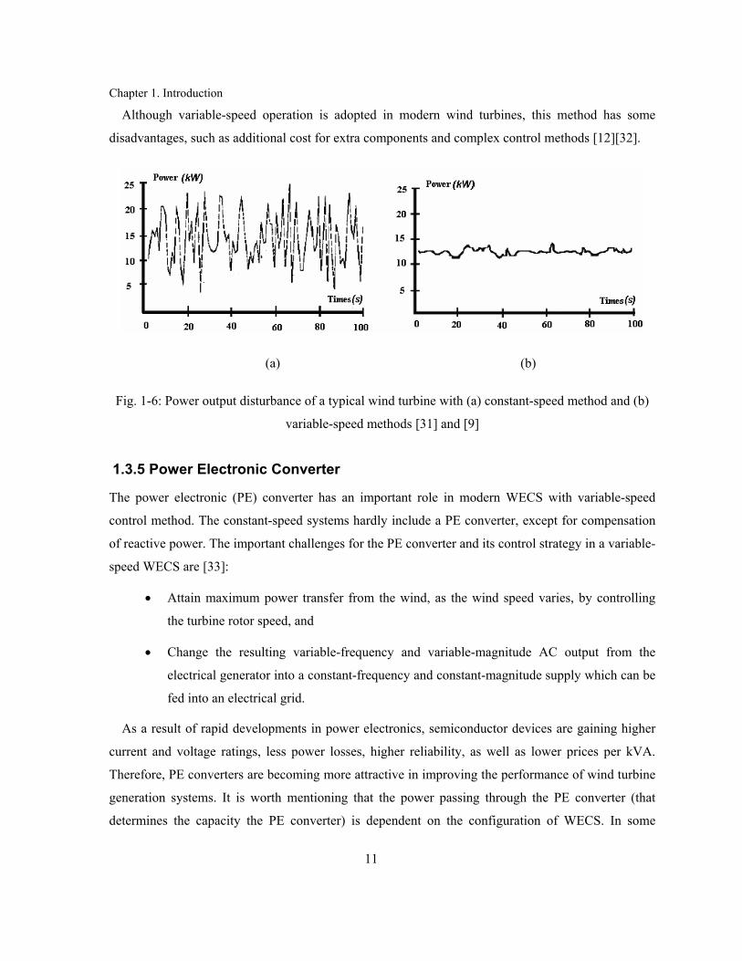
During turbine operation, there are some fluctuations related to mechanical or electrical
components. The fluctuations related to the mechanical parts include current fluctuations caused by
the blades passing the tower and various current amplitudes caused by variable wind speeds. The
fluctuations related to the electrical parts, such as voltage harmonics, is caused by the electrical
converter. The electrical harmonics can be conquered by choosing the proper electrical filter.
However, because of the large time constant of the fluctuations in mechanical components, they
cannot be canceled by electrical components. One solution that can largely reduce the disturbance
related to mechanical parts is using a variable-speed wind turbine. References [31] and [9] compare
the power output disturbance of a typical wind turbine with the constant-speed and variable-speed
methods, as shown in Fig. 1-6. The figure illustrates the ability of the variable-speed system to reduce
or increase the shaft speed in case of torque variation. It is important to note that the disturbance of
the rotor is related also to the mechanical inertia of the rotor.
Chapter 1. Introduction
11
Although variable-speed operation is adopted in modern wind turbines, this method has some
disadvantages, such as additional cost for extra components and complex control methods [12][32].
(a) (b)
Fig. 1-6: Power output disturbance of a typical wind turbine with (a) constant-speed method and (b)
variable-speed methods [31] and [9]
1.3.5 Power Electronic Converter
The power electronic (PE) converter has an important role in modern WECS with variable-speed
control method. The constant-speed systems hardly include a PE converter, except for compensation
of reactive power. The important challenges for the PE converter and its control strategy in a variable-
speed WECS are [33]:
• Attain maximum power transfer from the wind, as the wind speed varies, by controlling
the turbine rotor speed, and
• Change the resulting variable-frequency and variable-magnitude AC output from the
electrical generator into a constant-frequency and constant-magnitude supply which can be
fed into an electrical grid.
As a result of rapid developments in power electronics, semiconductor devices are gaining higher
current and voltage ratings, less power losses, higher reliability, as well as lower prices per kVA.
Therefore, PE converters are becoming more attractive in improving the performance of wind turbine
generation systems. It is worth mentioning that the power passing through the PE converter (that
determines the capacity the PE converter) is dependent on the configuration of WECS. In some

Chapter 1. Introduction
12
applications, the whole power captured by a generator passes through the PE converter, while in other
categories only a fraction of this power passes through the PE converter.
The most common converter configuration in variable-speed wind turbine system is the rectifier-
inverter pair. A matrix converter, as a direct AC/AC converter, has potential for replacing the
rectifier-inverter pair structure.
1.3.5.1 Back-to-back rectifier-inverter pair
The back-to-back rectifier-inverter pair is a bidirectional power converter consisting of two
conventional pulse-width modulated (PWM) voltage-source converters (VSC), as shown in Fig. 1-7.
One of the converters operates in the rectifying mode, while the other converter operates in the
inverting mode. These two converters are connected together via a dc-link consisting of a capacitor.
The dc-link voltage will be maintained at a level higher than the amplitude of the grid line-to-line
voltage, to achieve full control of the current injected into the grid. Consider a wind turbine system
including the back-to-back PWM VSC, where the rectifier and inverter are connected to the generator
and the electrical grid, respectively. The power flow is controlled by the grid-side converter in order
to keep the dc-link voltage constant, while the generator-side converter is responsible for excitation of
the generator (in the case of squirrel-cage induction generator) and control of the generator in order to
allow for maximum wind power to be directed towards the dc bus [82]. The control details of the
back-to-back PWM VSC structure in the wind turbine applications has been described in several
papers [33]-[36].
dcC
Rectifier Inverter
Fig. 1-7: The back-to-back rectifier-inverter converter
Among three-phase AC/AC converters, the rectifier-inverter pair structure is the most commonly
used, and thus, the most well-known and well-established. Due to the fact that many semiconductor
device manufacturers produce compact modules for this type of converter, the component cost has

Chapter 1. Introduction
13
gone down. The dc-link energy-storage element provides decoupling between the rectifier and
inverter. However, in several papers, the presence of the dc-link capacitor has been considered as a
disadvantage. The dc-link capacitor is heavy and bulky, increases the cost, and reduces the overall
lifetime of the system [37]-[40].
1.3.5.2 Matrix Converter
Matrix converter (MC) is a one-stage AC/AC converter that is composed of an array of nine
bidirectional semiconductor switches, connecting each phase of the input to each phase of the output.
This structure is shown in Fig. 1-8.
The basic idea behind matrix converter is that a desired output frequency, output voltage and input
displacement angle can be obtained by properly operating the switches that connect the output
terminals of the converter to its input terminals.
The development of MC configuration with high-frequency control was first introduced in the work
of Venturini and Alesina in 1980 [41][42]. They presented a static frequency changer with nine
bidirectional switches arranged as a 3×3 array and named it a matrix converter. They also explained
the low-frequency modulation method and direct transfer function approach through a precise
mathematical analysis. In this method, known as direct method, the output voltages are obtained from
multiplication of the modulation transfer matrix by input voltages [43]. Since then, the research on the
MC has concentrated on implementation of bidirectional switches, as well as modulation techniques.
Fig. 1-8: Matrix converter structure
One of practical problems in the implementation of MC is the use of four-quadrant bidirectional
switches. Using this type of switch is necessary for successful operation of MC. The earlier works

Chapter 1. Introduction
14
applied thyristors with external forced commutation circuits to implement the bidirectional controlled
switch [44][45], but this solution was bulky and its performance was poor. Monolithic four-quadrant
switches are not available to date. However, the introduction of power transistors provided the
possibility of implementing four-quadrant switches by anti-parallel connection of two two-quadrant
switches. Another problem in implementing MC is the switch commutation problem that produces
over-current, due to short circuiting of the ac sources, or over-voltage spikes, due to open circuiting
the inductive loads, that can destroy the power semiconductor. Safe commutation has been achieved
by the development of several multi-step commutation strategies and the “semi-soft current
commutation” technique [46]-[49].
A different modulation method that has been introduced in the literature is the indirect transfer
matrix based on a “fictitious dc link”. This method was introduced by Rodriguez in 1983 [50]. In this
method, based on the conventional PWM technique, at each switching period, each output line
connects two input lines that have maximum line-to-line voltage [51]. In 1986, Ziogas [52][53]
expanded this method by mathematical analysis. At the same time, another useful modulation method
that was introduced instead of PWM was space vector modulation [54][55]. In the next few years, the
principles of this method were developed for MC by researchers [56][57].
In 2001, a novel MC topology with a simple switching method, without commutation problems,
was developed by Wei and Lipo [58][59]. The improved matrix converter is based on the concept of
“fictitious dc link” used in controlling the conventional matrix converter. However, there is no energy
storage element between the line-side and load-side converters.
Nowadays, the operational and technological research on MC is continuing [60]. The following
items show the state of the art research on MC:
• New topology of MC [59][61],
• Safe and practical commutation strategies [62][63],
• Abnormal operational conditions [64][65],
• Protection issues and ride-through capability [66][67],
• New bidirectional switches and packaging [68][69],
• Input filter design [70][71], and
• New control methods [72][73].

Chapter 1. Introduction
15
1.3.5.3 Comparison of MC with the rectifier-inverter pair
As in the case of rectifier-inverter pair under PWM switching strategy, MC provides low-distortion
sinusoidal input and output waveforms, bi-directional power flow, and controllable input power factor
[74]. The main advantage of the MC is in its compact design which makes it suitable for applications
where size and weight matter, such as in aerospace applications [66][75].
The following drawbacks have been attributed to matrix converters: The magnitude of the MC
output voltage can only reach 0.866 times that of the input voltage, input filter design for MC is
complex, and because of absence of a dc-link capacitor in the MC structure the decoupling between
input and output and ride-through capability do not exist, limiting the use of MC [66][67][76].
In [77] and [78], the efficiencies of an MC and a rectifier-inverter pair with the same ratings are
compared. Based on the results, one can conclude that at low switching frequencies, the MC has
higher efficiency than the rectifier-inverter pair under PWM. However, adopting different modulation
schemes can reduce the switching losses in the rectifier-inverter pair [79]. In an MC, loss reduction is
possible by reducing the number of switchings [80] and using a modified SVM approach.
1.3.6 Different Configurations for Connecting Wind Turbines to the Grid
The connection of the wind turbine to the grid depends on the type of electrical generator and power
electronic converter used. Based on the application of PE converters in the WECS, the wind turbine
configurations can be divided into three topologies: directly connected to the grid without any PE
converter, connected via full-scale the PE converter, and connected via partially-rated PE converter.
In the following, the generator and power electronic converter configurations most commonly used in
wind turbine systems are discussed.
As a simple, robust and relatively low-cost system, a squirrel-cage induction generator (SCIG), as
an asynchronous machine, is connected directly to the grid, as depicted in Fig. 1-9. For an induction
generator, using a gearbox is necessary in order to interface the generator speed and turbine speed.
The capacitor bank (for reactive power compensation) and soft-starter (for smooth grid connection)
are also required. The speed and power are limited aerodynamically by stall or pitch control. The
variation of slip is in the range of 1-2%, but there are some wind turbines based on SCIG in industry
with increased rotor resistance and, therefore, increased slip (2-3%). This scheme is used to allow a
little bit of speeding up during wind gusts in order to reduce the mechanical stresses. However, this

Chapter 1. Introduction
16
configuration based on almost fixed speed is not proper for a wind turbine in a higher power range
and also for locations with widely varying wind velocity [8][81].
Gear Box
Reactive Compensator
GridSCIG
Fig. 1-9: Wind turbine system with SCIG
Three wind turbine systems based on induction generators, with the capability of variable-speed
operation are shown in Fig. 1-10 [8][19]. The wind turbine system in Fig. 1-10 (a) uses a wound-rotor
induction generator (WRIG). The idea of this model is that the rotor resistance can be varied
electronically using a variable external rotor resistance and a PE converter. By controlling the rotor
resistance, the slip of the machine will be changed over a 10% range (speed range 2-4%) [8]. In
normal operation, the rotor resistance is low, associated with low slip, but during wind gusts the rotor
resistance is increased to allow speeding up.
Fig. 1-10 (b) shows a configuration employing a Doubly-Fed Induction Generator (DFIG) and a
power electronic converter that connects the rotor winding to the grid directly. With this
configuration, it is possible to extend the speed range further without affecting the efficiency. The
reason for speed control without loss of efficiency is that slip power can be fed back to the grid by the
converter instead of being wasted in the rotor resistance. Note that the power rating of the power
converter is sPnom , where ‘s’ is the maximum possible slip and Pnom is the nominal power of the
machine. The rotor slip (s) can be positive or negative because the rotor power can be positive or
negative, due to the bidirectional nature of power electronic converter. For example, if the power
rating of the converter is 10% of the power rating of the generator, the speed control range is from
90% to 110% of the synchronous speed. It means at 110% speed, s=-0.1 and power is fed from the
rotor to the grid, whereas at 90% speed, the slip is s=+0.1, and 10% of the power is fed from the grid
to the rotor through the converter. With these attributes, i.e., a larger control range and smaller losses,
the configuration in Fig. 1-10 (b) is more attractive than the configuration in Fig. 1-10 (a).

Chapter 1. Introduction
17
G ea r B o x
R eactiv e C o m p en sator
G rid
W R IG
R esista n ce co n tro l b y P E C
(a )
G ea r B o x
D F IG
(b )
G rid
_~_~
G ea r B o x
B D F IG
(c )
G rid
_~_~
Fig. 1-10: Wind turbine systems based on induction generator with capability of variable-speed
operation: (a) Wound-Rotor, (b) Doubly-Fed, and (c) Brushless Doubly-Fed induction generators
In the configurations shown in Fig. 1-10 (a) and Fig. 1-10 (b), with wound-rotor induction
generator, the access to the rotor is possible through the slip rings and brushes. Slip rings and brushes
cause mechanical problems and electrical losses. In order to solve the problems of using slip rings and
brushes one alternative is using the Brushless Doubly-Fed induction generator (BDFIG), shown in
Fig. 1-10 (c). In this scheme, the stator windings (main winding) are directly connected to the grid,
while the three-phase auxiliary winding is connected to the electrical grid through a PE converter. By
using the appropriate control in the auxiliary winding, it is possible to control the induction machine
at almost any speed. Also, in this configuration, a fraction of the generator power is processed in the
converter.
In the third category, the electrical machine is connected to the electrical grid via a fully-rated
converter. It means that the whole power interchanged between the wind turbine and the electrical
grid must be passed through a PE converter. This implies extra losses in the power conversion.
However this configuration will improve the technical performance. In this configuration, as an
electrical machine, it is possible to use induction machine or synchronous machine, as shown in Fig.

Chapter 1. Introduction
18
1-11 [8][19][82]. Note that the system of Fig. 1-11 (a) uses a gearbox together with a SC induction
generator. The systems of Fig. 1-11 (b) and (c) use synchronous generators without a gear box.
The configuration in Fig. 1-11 (b) the synchronous generator needs a small power electronic
converter for field excitation, and slip rings. An advantage of using the synchronous generator is the
possibility of eliminating the gearbox in the wind turbine (direct-drive wind turbine). Direct drive
generators essentially have a large diameter because of the high torque. In gearless drives, induction
machines cannot be used because of the extreme excitation losses in these large machines due to the
large air gap. However, synchronous machines can be used in direct-drive wind turbines, with either
electrically excited or permanent-magnet rotor structures (Fig. 1-11 (c)). Direct-drive systems with
permanent magnet excitation are more expensive, because of the high price of magnets, but have
lower losses. Nowadays, the price of permanent magnets is decreasing dramatically. Another
disadvantage of using permanent magnet synchronous machine is the uncontrollability of its
excitation.
All configurations shown in Fig. 1-11 have the same control characteristics since the power
converter between the generator and the grid enables fast control of active and reactive power. Also,
the generator is isolated from the grid by a dc-link capacitor. But, using fully-rated power electronic
converter is the disadvantage of these configurations.
Different wind turbine manufacturers produce different configurations. Comparing different
systems from different points of view shows a trade-off between cost and performance.
1.3.7 Starting and disconnecting from electrical grid
When wind velocities reach approximately 7 miles per hour wind turbine’s blades typically start
rotating, but, at 9 to 10 mph, they will start generating electricity. To avoid damage, most turbines
automatically shut themselves down when wind speeds exceed 55 to 65 mph. When the wind turbines
are connected to or disconnected from the grid, voltage fluctuation and transient currents can occur.
The high current can be limited using a soft-start circuit [22].

Chapter 1. Introduction
19
GearBox
Grid
IG
(a)
Multi-pole SG
(b)
_
~
(c)
~~ __
QrefPref
Grid
~_
QrefPref
~
_
Multi-pole PM-SG
_Grid
~_
QrefPref
~
Fig. 1-11: Wind turbine systems with fully-rated power converter between generator terminals and
the grid: (a) induction generator with gearbox, (b) synchronous and, (c) PM synchronous generator
1.4 Literature Survey on Using Matrix Converters in Wind Turbine Systems
Some researchers have adopted MC as a PE converter in variable-speed wind turbine systems. In
reference [83], an MC is used to interface the grid and the induction generator. A closed-loop speed
observer is adopted to estimate the generator variables, i.e., shaft speed, generator active power, and
stator flux. The main drawback of this method is using an observer that dramatically decreases the
gain and phase margin of the system. Also, the closed-loop system needs a reference for the stator
flux. Furthermore, the system does not include maximum power point tracking.
A variable-speed wind turbine system with a DFIG, using an MC in the rotor circuit has been
presented in [84]. In this system, the MC is used to control the DFIG based on a sliding mode control
technique to extract the maximum energy from the wind. The induction generator can operate under

Chapter 1. Introduction
20
or above the synchronous speed with a smooth operation. However, the system needs a stator flux
estimator to obtain the current reference. Adding a flux observer adds complexity to the system.
In [85]-[89], the advantages of an MC and a brushless doubly-fed machine (BDFM) are combined
in a variable-speed wind turbine system. In these papers, an MC is used to control the generator and
capture the maximum energy from the wind. A field-oriented vector control method is used in [85] to
control a BDFM in order to capture maximum wind energy and improve the generated electric power
quality. The output frequency of the BDFM is kept constant and the output power regulated by
controlling the exciting voltage of control winding when the shaft speed of machine varies. This
topology needs a turbine shaft speed sensor as well as power and flux estimators. In [86]-[89], the
control of BDFM is based on field-oriented vector control and a decoupling control of the active and
reactive powers of the generator. The control method suffers from a number of drawbacks due to
measuring a lot of variables such as: wind velocity, generator shaft speed, stator and rotor currents,
and rotor voltage.
1.5 Thesis Objectives
Based on the state-of-the-art in wind energy conversion research discussed above, this work aims to
investigate the application of MC in wind energy conversion systems for two reasons: first, MC is an
emerging technology with the potential of replacing rectifier-inverter pair, and second, no thorough
study of this application has been made.
The main objectives of this thesis are as follows:
1- Developing a low-to-medium-power (below 1MW), variable-speed wind turbine system based
on a matrix converter and an induction generator,
2- Adopting the MC control functions to control active and reactive powers injected into the grid,
3- Developing a comprehensive dynamic model for the MC to satisfy all functions of the MC,
including the control of the displacement power factor,
4- Developing a comprehensive dynamic mathematical model for the wind turbine system
including MC to be used for controller design purposes,
5- Control of the induction machine based on constant V/f strategy to avoid saturation of the
induction generator,

Chapter 1. Introduction
21
6- Designing a state-feedback and an output-feedback controller for the system to improve the
system performance, and
7- Developing a maximum power point tracking method to vary MC control variables in order to
capture maximum wind energy, without measuring the wind velocity or the mechanical speed
of turbine shaft.
1.6 The Proposed Wind Energy Conversion System
Based on the objectives stated in the previous section, a wind energy conversion system based on a
squirrel cage induction generator (SCIG) and an MC is proposed. Fig. 1-12 shows the block diagram
of the proposed wind energy conversion system.
Fig. 1-12: Block diagram of the proposed wind energy conversion system
The SCIG is a low-cost and robust machine and the industry has a lot of experience in dealing with
it. In addition, the induction generator has high reliability and the right mechanical properties for
wind turbines, such as slip and a certain degree of overload capability. These are the main reasons for
choosing this type of generator in the proposal system.
The wind turbine is followed by a gearbox which steps up the shaft speed. Note that working at a
low shaft speed translates into a low induction generator terminal frequency which can result in core
saturation unless a low terminal voltage is imposed. At low terminal voltages, the operating current
will be high, making the scheme impractical.
As a power electronic converter, a matrix converter is used. MC interfaces the SCIG with the grid
and implements shaft speed control. In the proposed system, the MC input is connected to the grid
and the generator terminals are connected to the MC output. The MC provides direct AC/AC
conversion and is considered an emerging alternative to the conventional two-stage AC/DC/AC

Chapter 1. Introduction
22
converter. MC is highly controllable and allows independent control of the output voltage magnitude,
frequency, and phase angle, as well as input power factor. Compared with the dc-link AC/AC
converter system, an advantage of MC is the elimination of the dc-link, including bulky capacitors.
Therefore, it can be recognized as a full-silicon structure in a compact design. Furthermore, the
structure is inherently capable of four-quadrant operation.
The space vector pulse width modulation (SVPWM) technique can be applied to control the
switching in an MC, and some solutions such as a four-step switching method and the improved MC
topology can be adopted to solve the commutation problem.
The closed-loop controller adjusts the MC controller variables in order to improve the system
steady-state and transient performance. The controller including the MPPT method controls the shaft
speed to maximize the power captured from the wind.
1.7 Thesis Outline
Chapter 2 is dedicated to development and validation of a comprehensive dynamic model for MC in
the qdo reference frame.
Chapter 3 presents an overall nonlinear dynamic mode for the proposed system in the qdo reference
frame. The final model is expanded to include the constant V/f strategy. Based on the overall model, a
linearized model is developed to investigate local stability and system performance.
Chapter 4 discusses the design of a closed-loop feedback controller based on the linear model. A
state-feedback controller with observer is designed for the system and evaluated. Then, to improve
the system performance, two other controllers based on transfer function techniques are designed.
Chapter 5 starts with introducing three different MPPT methods, i.e., Perturbation and Observation
(P&O), Wind Speed Measuring (WSM), and Power Signal Feedback (PSF). Then, the mechanical
speed-sensorless PSF method is developed for the wind turbine system under study.
Chapter 6 summarizes the thesis main points and contributions, and proposes future directions for
research.
Finally, the thesis ends with appendixes as listed in the table of contents.

23
Chapter 2
Matrix Converter Structure and Dynamic Model
2.1 Introduction
Power electronic converters (PECs) play two important roles in modern variable-speed wind energy
conversion systems: interfacing the wind turbine to the electrical utility grid and controlling the wind
turbine. A static frequency changer can satisfy the requirements of a variable-speed wind turbine. The
two main structures that are suitable for this application are: dc-link AC/DC/AC converter and matrix
converter (MC). The most common power electronic configuration for SCIG-based variable-speed
WECS is an AC/DC/AC converter with a large dc-link capacitor.
The MC provides direct AC/AC conversion and is considered an emerging alternative to the
conventional two-stage AC/DC/AC converter topology [60][66]. An MC offers a high degree of
controllability that allows independent control of the output voltage magnitude, frequency, and phase
angle, as well as the input power factor. When compared with the dc-link AC/DC/AC converter
system, a principal feature of the MC is elimination of the dc-link and the bulky capacitors.

Chapter 2. Matrix Converter …
24
In the proposed system, the MC controls the terminal voltage and frequency of the induction
generator in such way that the wind turbine is operated at its maximum power point. In addition, the
MC implements unity power factor at the interface with the grid. This system targets small-to-
medium-power wind turbines.
In this chapter, first the MC topology and its switching method is introduced. Then a
comprehensive dynamic model for the MC will be developed which is valid for both steady-state and
transient analyses. The comprehensive model satisfies all normal functions of MC, i.e., control of the
output voltage magnitude, output frequency, and input displacement power factor. The developed
model is in qdo reference frame and is based on the MC input and output voltage and current
fundamental components. The validity of this model will be confirmed by comparing the results
obtained from the model with those obtained from a simplified fundamental-frequency equivalent
circuit-based model and the simulation results from PSIM simulation package.
2.2 Static Frequency Changer (AC/AC Converter)
A static frequency changer is a converter which can convert ac power at a given frequency to ac
power at a different frequency. In this conversion, voltage magnitude and phase angle can be
controlled as well. Fig. 2-1 shows the block diagram of a three-phase to three-phase static frequency
changer. The side-1 of the static frequency changer is connected to a three-phase ac power supply
with balanced sinusoidal voltages at the frequency f1, voltage magnitude V1 and phase angle φ1, while
a three-phase load is connected on side-2. The frequency changer converters the three-phase balanced
sinusoidal voltage on side-1 to a three-phase balanced sinusoidal system on side-2 at new electrical
characteristics, frequency f2, voltage magnitude V2 and voltage phase angle φ2 [90].
Static Frequency Changer
Va
Vb
Vc
ia
ib
ic
3-PHLoad
VA
VB
VC
iA
iB
iC
Side-1 Side-2 With (f2, V2 , 2 )With (f1, V1 , 1 )
Fig. 2-1: Block diagram of a three-phase to three-phase static frequency changer
From the viewpoint of structure, static frequency changers are divided into two categories: two-
stage or rectifier-inverter pair (indirect topology), and single-stage (direct topology). The term direct

Chapter 2. Matrix Converter …
25
means that the energy does not appear in the form of dc in the conversion process. Therefore,
electrical energy can be transferred between the input and output of the converter without a dc-link. A
single-stage static frequency changer can be realized by thyristors. In that case, it is called a naturally-
commutated cycloconverter, featuring restricted frequency conversion. It is also possible to realize a
single-stage static frequency changer by controllable switches. In this case, it is called a forced-
commutated cycloconverter or a Matrix Converter (MC).
2.3 Matrix Converter Structure
The structure of a MC is shown in Fig. 2-2 and the parameters of the circuit are defined in Table 2.1
The MC connects the three-phase ac voltages on input side to the three-phase voltages on output side
by a 3×3 matrix (or array) of bi-directional switches. In total, MC needs 9 bi-directional switches, one
switch between each input phase and each output phase. A second-order L-C filter is used at the input
terminals to filter out the high frequency harmonics of the input currents [90]-[92].
The MC, as an AC/AC converter, satisfies the requirement of providing a sinusoidal voltage on the
load side and a sinusoidal current on the source side. Meanwhile, it is possible to adjust the input
displacement angle and control the output voltage magnitude and phase angle by properly operating
the switches. Since there is no dc-link as compared with a two-stage conventional AC/DC/AC
converter, MC can be recognized as a full-silicon structure in a compact design. Also, the structure is
inherently capable of a four-quadrant operation, with the output voltage and input current sinusoidally
shaped with low distortion.
The disadvantages of a MC are in the high number of devices in the power circuit (18 switches and
18 diodes) and complexity of topology. Appendix A explains the practical switch configurations and
compares the bidirectional switch structures for the MC.

Chapter 2. Matrix Converter …
26
aii
bii
cii
C_a inv
_b inv _c inv
iR iLai
bi
ci
av
bv
cv Ci
_C outv _B outv _A outv
oR oL
Bi
AiAv
Bv
Cv
AbS
AcS
BaS
BbS
BcS
CaS
CbS
CcS
AaS
Fig. 2-2: A matrix converter circuit
Table 2.1: Parameters of the MC circuit.
Parameters Descriptions
vi, ii (i=a,b,c) vj, ij (j=A,B,C) vi_in, (i=a,b,c) vj_out (j=A,B,C) Ri Li C Ro Lo
Sij (i=a,b,c, j=A,B,C )
Three-phase MC input voltages and currents Three-phase MC output voltage and currents Three-phase input voltage sources Three-phase output voltage sources Input source resistance per phase Input source plus filter inductance per phase Input filter capacitor per phase per phase Output source resistance per phase Output source inductance Switch between phase i and phase j

Chapter 2. Matrix Converter …
27
2.4 Modulation Strategy for the Matrix Converter
In the MC the switching method should be chosen in such a way that the output voltages have
sinusoidal waveforms at the desired frequency, magnitude and phase angle. Also, the input currents
should be sinusoidal at the desired displacement power factor. In order to achieve this target, a proper
choice of the switching pattern should be applied to the switches of the MC in a switching period. A
proper switching pattern is obtained by choosing a suitable modulation method. The modulation
problem in general starts with choosing a switching function for the switches of the MC as follows
[60][93]:
1 ,( ) , , , , , , .
0 ,ij
ijij
S closedS t i A B C j a b c
S open= = =⎧⎪⎨⎪⎩
(2.1)
The following constraint applies to the switching functions:
1, , , .ia ib icS S S i A B C+ + = = (2.2)
This constraint comes from the fact that MC is supplied from a voltage source and generally feeds
an inductive load. Connecting more than one input phase to one output phase causes a short circuit
between two input sources (Fig. 2-3(a)). Also, disconnecting all input phases from an output phase
results in an open circuit in the load (Fig. 2-3 (b)) [55].
Fig. 2-3: Undesirable situations in MC: (a) short circuit of input sources (b) open circuit of inductive
load

Chapter 2. Matrix Converter …
28
By considering two states for each switching function based on (2.1), there are 512 states for a total
of 9 switches in the MC. By applying the constraint (2.2) to the switching algorithms of the MC of
Fig. 2-2, only 27 allowable combinations can exist. These switching state combinations are shown in
Appendix B.
Finding a proper modulation strategy for MC starts with considering a set of input and output
voltages and currents, based on MC circuit of Fig. 2-2, as follows:
an
abc bn
cn
vv v
v
⎡ ⎤⎢ ⎥= ⎢ ⎥⎢ ⎥⎣ ⎦
, AN
ABC BN
CN
vv v
v
⎡ ⎤⎢ ⎥= ⎢ ⎥⎢ ⎥⎣ ⎦
, a
abc b
c
ii i
i
⎡ ⎤⎢ ⎥= ⎢ ⎥⎢ ⎥⎣ ⎦
, A
ABC B
C
ii i
i
⎡ ⎤⎢ ⎥= ⎢ ⎥⎢ ⎥⎣ ⎦
, (2.3)
where abcv and ABCv are the MC input and output phase-to-neutral voltage vectors, and abci and ABCi
are the MC input and output current vectors.
Based on the definition of switching function given by (2.1), the MC instantaneous switching
function matrix is as follows [90]-[95]:
.Aa Ab Ac
Ba Bb Bc
Ca Cb Cc
s s sS s s s
s s s
⎡ ⎤⎢ ⎥= ⎢ ⎥⎢ ⎥⎣ ⎦
(2.4)
The input-side and output-side voltages and currents are related by the following equations:
ABC abcv S v= ⋅ , and .Tabc ABCi S i= , (2.5)
where ST is the transpose of S. The elements of S should be chosen properly to obtain the desired
fundamental components of output voltages and input currents. This means that in a certain period of
time, the switches of the MC have to be turned on and off according to a specific switching pattern.
Assuming that the switching frequency is much higher than the input and output frequencies, the
switching functions can be replaced by their low-frequency components, as far as the fundamental
components of input-side and output-side voltages and currents are concerned. Based on this, the
switching functions in S can be replaced by the ‘duty cycles’ of switches. The duty cycle is defined
as:

Chapter 2. Matrix Converter …
29
( ) , , , , , ,ijij
Seq
td t i A B C j a b c
T= = = (2.6)
where tij is the ON period of the switch ij in a switching sequence time. For example, as illustrated in
Fig. 2-4, during a certain sequence period Tseq, the output phase “A” is connected to input phase “a”
during time period tAa and is connected to phase ‘b’ and ‘c’ during time periods tAb and tAc ,
respectively [60].
seqT
1=AaS
Aat1=AbS 1=AcS
Abt Act1=BaS 1=BbS 1=BcS
Bat Bbt Bct1=CaS 1=CbS 1=CcS
Cat CbtCct
Fig. 2-4: The switching pattern in a sequence period
The following two restrictions apply to the duty cycle based on the (2.2):
0 1, ( , , ), ( , , ).
1ji
ja jb jc
dj A B C i a b c
d d d≤ ≤
∈ ∈+ + =
⎧⎨⎩
(2.7)
By considering the duty cycles of the switches, the matrix S can be replaced by matrix D, given by
(2.8), where elements are the low-frequency components (or local averages) of S matrix elements.
.Aa Ab Ac
Ba Bb Bc
Ca Cb Cc
d d dD d d d
d d d
⎡ ⎤⎢ ⎥= ⎢ ⎥⎢ ⎥⎣ ⎦
(2.8)
The matrix D is called modulation matrix or low-frequency transformation matrix.
The solution to the modulation problem is that of finding the elements of matrix D in such a way
that the desired output voltage and input current vectors are obtained, and the restrictions given by
(2.7) are satisfied. Therefore the equation (2.5) can be rewritten as [91][93][94]

Chapter 2. Matrix Converter …
30
ABC abcv D v= ⋅ , and .Tabc ABCi D i= , (2.9)
where abcv and ABCi are a set of sinusoidal input voltages and output currents, and ABCv and abci are
the desired fundamental-frequency output voltages and input currents at the MC terminals.
Based on the concept of high-frequency switching and low-frequency transfer function, the
following steps should be taken in finding a control method for the MC:
• choosing a modulation algorithm based on the structure of the transformation matrix,
• finding a proper duty cycle formula, dij, for switching to realize the transformation
matrix and satisfy the duty cycle restrictions, given by equation (2.7), and
• determining the states of the nine switches in the MC in each sequence period based on
the duty cycle.
Appendix C is dedicated to describing two major modulation algorithms, i.e., direct and indirect
approaches. The indirect method, which is based on the concept of fictitious rectifier-inverter pair and
dc-link, is an appropriate method for implementing Pulse Width Modulation (PWM) and Space
Vector PWM (SVPWM) techniques. The details of the (SVPWM) technique are given in Appendix
C. In addition, a comparison between PWM and SVPWM modulation techniques is presented in
Appendix D.
2.5 Commutation Problems in Matrix Converter
As mentioned in previous section, in order to avoid short circuiting the input lines, no two
bidirectional switches should be switched on to the same output phase at any instant. Also, for
preventing an open circuit in inductive load on the output side of the MC, bidirectional switches
linked to the same output phase should not all be turned off at any instant. Since practical
semiconductor switches have propagation delays and finite switching times, switches cannot be
switched on and off instantaneously. These two issues are commutation problems in the MC that are
more difficult to overcome than in conventional voltage source converters. The following two
solutions have been pointed out in the literatures for the commutation problems in MC:
• Safe commutation in switching sequence
• Indirect MC topology
Appendix E is dedicated to describing these solutions.

Chapter 2. Matrix Converter …
31
2.6 Simulation Results of the Matrix Converter Based on SVPWM
In this section, the simulation results of a MC circuit, Fig. 2-2, using the SVPWM technique are
presented. Fig. 2-5 illustrates the MC circuit set up in PSIM environment. This circuit is implemented
in MC module of Fig. 2-6. This figure shows the whole system required for simulation of the MC
based on the SVPWM technique. The DLL block executes the SVPWM method and contains four
control variables (or desired values) that can be used to control the MC output voltage magnitude,
frequency and phase angle, as well as the input displacement angle.
As an example to assess the performance of MC of Fig. 2-6, the input source characteristics,
control variables and load characteristics are set as follows:
• Input Source: Vin-peak=140V (Phase-to-Neutral), fin=60Hz,
• MC control variables: Voltage gain = 0.571, output frequency =75Hz, output voltage angle=0, input displacement power factor=1, and
• Load: Three-phase RL load (Y-connected), Rload=20Ω, Lload=50mH (all per phase). Fig. 2-7 shows the results of simulation. As shown in the figure, the fundamental components of
the output line-to-line voltages, output currents and input currents are sinusoidal. The simulation
results confirm that the desired values for the output frequency, voltage magnitude and phase angle,
as well as the input displacement angle are achievable. Fig. 2-7 (a) shows the output frequency is 75
Hz. Also, Fig. 2-7 (d) illustrates that the input phase current and voltage are in-phase, due to the fact
that the input displacement angle is set to zero.

Chapter 2. Matrix Converter …
32
Fig. 2-5: Implementing MC circuit in PSIM environment
Fig. 2-6: Implementing the whole MC system in PSIM environment for simulation based on the SVPWM
technique, DLL block executes the SVPWM method

Chapter 2. Matrix Converter …
33
Fig. 2-7: Simulation results of the MC: (a) output line-to-line voltages, (b) phase-A output current, iA,
(c) phase-a input current, ia, and (d) phase-a input phase voltage, va , and input current fundamental
component, ia1.

Chapter 2. Matrix Converter …
34
2.7 An Overall Dynamic Model for a the Matrix Converter System
In this section, a comprehensive dynamic model for a matrix converter (MC) is developed which is
valid for both steady-state and transient analyses. The comprehensive model includes all normal
functions of the MC, i.e., control of the output voltage magnitude, output frequency, and input
displacement power factor. The model is in the qdo reference frame for the MC input and output
voltage and current fundamental components. The validity of this model is confirmed by comparing
the results obtained with those of a simplified fundamental-frequency equivalent circuit-based model
and the simulation results from PSIM package.
2.7.1 Low- Frequency Transformation Matrix
As mentioned in section 2.4, as far as the fundamental components of the MC input and output
voltages and currents are concerned, the switching function matrix S can be replaced by the
transformation matrix D. The transformation matrix D should satisfy the following three
requirements:
(a) restrictions on duty cycle, described by equation (2.2),
(b) sinusoidal output voltages with controllable frequency, magnitude and phase angle,
(c) sinusoidal input currents,
(d) desired input displacement power factor.
The following low-frequency transformation matrices are two basic solutions that individually satisfy
the requirements (a), (b) and (c) [55][60][91][93][94].
1 1 1
1 1 1 1
1 1 1
1 2 cos( ) 1 2 cos( 2 / 3) 1 2 cos( 2 / 3)1 1 2 cos( 2 / 3) 1 2 cos( ) 1 2 cos( 2 / 3)3
1 2 cos( 2 / 3) 1 2 cos( 2 / 3) 1 2 cos( )
s s s
s s s
s s s
q q qD q q q
q q q
θ θ π θ πθ π θ θ πθ π θ π θ
+ + − + +⎡ ⎤⎢ ⎥= + + + + −⎢ ⎥⎢ ⎥+ − + + +⎣ ⎦
(2.10)
2 2 2
2 2 2 2
2 2 2
1 2 cos( ) 1 2 cos( 2 / 3) 1 2 cos( 2 / 3)1 1 2 cos( 2 / 3) 1 2 cos( 2 / 3) 1 2 cos( )3
1 2 cos( 2 / 3) 1 2 cos( ) 1 2 cos( 2 / 3)
s s s
s s s
s s s
q q qD q q q
q q q
θ θ π θ πθ π θ π θθ π θ θ π
+ + − + +⎡ ⎤⎢ ⎥= + − + + +⎢ ⎥⎢ ⎥+ + + + −⎣ ⎦
(2.11)
where 1 ( )s i o ot tθ ω ω α= − + , 2 ( )s i o ot tθ ω ω α= + + , ii fπω 2= , if : MC input frequency, oo fπω 2= ,
of : output frequency of the MC, :oα output voltage angle of the MC (input voltage angle as a

Chapter 2. Matrix Converter …
35
reference), and q=Vom/Vim: MC output-to-input voltage gain. Note that 87.00 ≤≤ q and Vom and Vim
are peak values of output and input voltage magnitudes.
It is worth mentioning that matrices D1 and D2 satisfy the duty cycle restriction, giving by equation
(2.2), and are invertible, a property useful for future calculations.
Note that neither D1 nor D2 alone can control the input displacement power factor. In fact, matrix
D1 gives the same phase displacement at the input as at the output, whereas matrix D2 yields a phase
displacement at the input equal in magnitude and opposite in sign to that at the output [94][95].
However, the combination of the two transformation matrices given by (2.12) provides controllability
of input displacement power factor.
1 2(1 )D aD a D= + − . (2.12)
In (2.12), a is a constant parameter varying between 0 and 1(0 1a≤ ≤ ).
In order to get a unity displacement power factor at the MC input terminals, the parameter a should
be set at 0.5. Note that this dose not result in a unity displacement power factor at input source
terminals.
2.7.2 Output voltage and input current of Matrix Converter
To find the output terminal voltage and input terminal current, consider the low-frequency
transformation function (2.12) and a set of sinusoidal input voltages, as follows:
cos( )cos( 2 / 3)cos( 2 / 3)
i
abc im i
i
tv V t
t
ωω πω π
⎡ ⎤⎢ ⎥= −⎢ ⎥⎢ ⎥+⎣ ⎦
, (2.13)
where oϕ is the output (or load) angle. Using equation (2.9), the MC output voltages can be written as
follows:
1 2
cos( )( ( 1) ) cos( 2 /3)
cos( 2 /3)
o o
ABC abc abc im o o
o o
tv Dv aD a D v qV t
t
ω αω α πω α π
+⎡ ⎤⎢ ⎥= = + − = + −⎢ ⎥⎢ ⎥+ +⎣ ⎦
. (2.14)
The output currents will be therefore be:
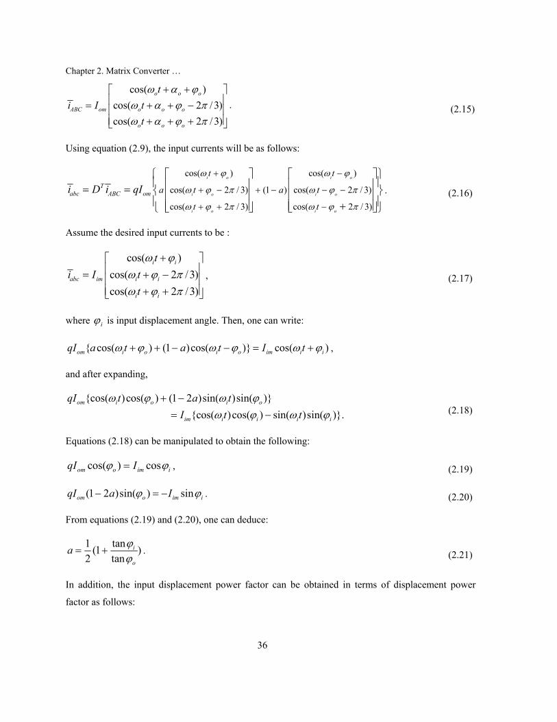
Chapter 2. Matrix Converter …
36
cos( )cos( 2 /3)cos( 2 /3)
o o o
ABC om o o o
o o o
ti I t
t
ω α ϕω α ϕ πω α ϕ π
+ +⎡ ⎤⎢ ⎥= + + −⎢ ⎥⎢ ⎥+ + +⎣ ⎦
. (2.15)
Using equation (2.9), the input currents will be as follows:
cos( ) cos( )
cos( 2 / 3) (1 ) cos( 2 / 3)
cos( 2 / 3) cos( 2 / 3)
i o i o
i o i o
i o i o
Tabc ABC om
t t
a t a t
t t
i D i qIω ϕ ω ϕ
ω ϕ π ω ϕ π
ω ϕ π ω ϕ π
+ −
+ − + − − −
+ + −
⎧ ⎡ ⎤ ⎡ ⎤⎫⎪ ⎪⎢ ⎥ ⎢ ⎥= = ⎨ ⎬⎢ ⎥ ⎢ ⎥⎪ ⎪+⎢ ⎥ ⎢ ⎥⎩ ⎣ ⎦ ⎣ ⎦⎭
. (2.16)
Assume the desired input currents to be :
cos( )cos( 2 /3)cos( 2 /3)
i i
abc im i i
i i
ti I t
t
ω ϕω ϕ πω ϕ π
+⎡ ⎤⎢ ⎥= + −⎢ ⎥⎢ ⎥+ +⎣ ⎦
, (2.17)
where iϕ is input displacement angle. Then, one can write:
cos( ) (1 )cos( ) cos( )om i o i o im i iqI a t a t I tω ϕ ω ϕ ω ϕ+ + − − = + ,
and after expanding,
cos( )cos( ) (1 2 )sin( )sin( )cos( )cos( ) sin( )sin( ).
om i o i o
im i i i i
qI t a tI t t
ω ϕ ω ϕω ϕ ω ϕ
+ −= −
(2.18)
Equations (2.18) can be manipulated to obtain the following:
cos( ) cosom o im iqI Iϕ ϕ= , (2.19)
(1 2 )sin( ) sinom o im iqI a Iϕ ϕ− = − . (2.20)
From equations (2.19) and (2.20), one can deduce:
1 tan(1 )2 tan
i
o
a ϕϕ
= + . (2.21)
In addition, the input displacement power factor can be obtained in terms of displacement power
factor as follows:

Chapter 2. Matrix Converter …
37
1 1costan [(21 1) tan(cos ( ))]in outDPF DPF− −= − , (2.22)
where cos( )in iDPF ϕ= and cos( )out oDPF α= are the input and output displacement power factors.
Equation (2.22) shows the variation of input displacement power factor as a function of parameter a
and output displacement power factor.
2.7.3 Matrix Converter Equivalent Circuit Model
Based on to the transformation matrix given by (2.12), MC can be represented by dependent current
and voltage sources at the input and output terminals, respectively. In fact, the voltage and current
dependent sources model the MC transformation matrix. This fundamental-frequency equivalent
circuit is shown in Fig. 2-8, corresponding to the MC circuit in Fig. 2-2 [94]. In comparison with
other MC equivalent-circuit models proposed in literature [92], the model of Fig. 2-8 is new in the
sense that it uses the transformation matrix given by (2-12). This model will be used as a reference
model to verify the state-space model developed in section 2.8.
_ABC outv
oR oLiR iL
C_abc inv
_A outva ii Ai_a inv
ai
ci
bib ii_b inv
_c invc ii
Av
Bv
Cv
_B outvBi
_C outvCi
Fig. 2-8 : One-line, fundamental-frequency equivalent circuit of the MC system
2.7.4 Evaluation of Matrix Converter Equivalent Circuit Model
In this subsection, first the MC equivalent circuit model of Fig. 2-8 is evaluated. For this purpose, a
typical MC system (Fig. 2-2) that is connected to two electrical systems with different frequencies
and impedances is simulated. For simplicity, the side-2 system is considered to be a passive load. The

Chapter 2. Matrix Converter …
38
MC is assumed to be composed of ideal switches and is controlled by the SVPWM switching method,
referred to as MC-SVM from now on. Then the simulation results are compared with those obtained
from simulation of the MC equivalent circuit (Fig. 2-8). Both circuits are simulated in the PSIM
environment. The schematic diagrams of the fundamental-frequency equivalent circuit and MC-SVM
system in PSIM are illustrated in Fig. 2-9 and Fig. 2-6, respectively. For both systems, the source at
the input-side is represented by three-phase sinusoidal voltages. To be consistent with MC-SVM
system in Fig. 2-6, the equivalent circuit model (Fig. 2-8) contains a simple three-phase passive load,
with resistance RLoad and inductance LLoad, on the output side. The parameters of the MC system are
shown in Table 2.2. In the following, selected simulation results of the MC equivalent system are
presented.
Fig. 2-9: Schematic diagram of the equivalent circuit in PSIM environment; the DLL block simulates
the transformation matrix D
Table 2.2: Parameters of the simulated MC system
Input System Output System Matrix Converter
Vph_in= 110 [V], Ri= 0.1[Ω]
Li = 0.1 [mH], C=20[µF]
fi=60[Hz]
Ro== 0.1[Ω], Li = 0.1 [mH]
RLoad== 0.1[Ω], Lload = 0.1 [mH]
fo=50[Hz]
Voltage gain q=0.5
Output voltage angle αo=0
Switching frequency=5 [kHz]
Fig. 2-10 shows the line-to-line output voltage waveforms of MC from the two models. For the
MC-SVM system, the output voltage is pulsed; however, its fundamental component has the same

Chapter 2. Matrix Converter …
39
frequency and approximately the same magnitude as the output voltage of the equivalent-circuit
model.
The waveforms input source currents for the two systems are illustrated in Fig. 2-11. The input
source current of the MC-SVM is a pulsed waveform; however, as shown in Fig. 2-11, the
corresponding source current is a sinusoidal with the same magnitude as the MC input source current
of the equivalent circuit MC model.
The active and reactive powers at the input and output terminals, as well as the input displacement
power factors are compared in Table 2.3. Based on the data presented in Table 2.3, there are minor
differences between the active powers of the two models. This is because of the minor difference
betweens the magnitude of input current and output voltage waveforms in the two models. However,
there is a rather large difference between the output reactive powers of the two models. The main
reason for this is the inclusion of harmonic components in the output voltage of MC-SVM model in
calculation of output reactive power, whereas in the equivalent-circuit MC model, only the
fundamental component of the output voltage has been considered. Filtering the output voltage signal
of MC-SVM model before reactive power calculation should bring the results much closer.
0.1 0.105 0.11 0.115 0.12 0.125 0.13 0.135 0.14 0.145 0.15-150
-100
-50
0
50
100
150
t[sec]
V[V]
Line-to-line Output volatge for SVM-MC and Equivalent-Circuit model
MC-SVM MC-SVM FundementalEquivalent-Circuit MC
Fig. 2-10: Line-to-Line output voltages of the MC-SVM and equivalent-circuit models.

Chapter 2. Matrix Converter …
40
0.1 0.105 0.11 0.115 0.12 0.125 0.13 0.135 0.14 0.145 0.15-5
-4
-3
-2
-1
0
1
2
3
4
5
t[sec]
I[Am
p.]
Input source current of the MC system
MC-SVMEquivalent-Circuit MC
Fig. 2-11: Phase-a input source currents of the MC-SVM and equivalent-circuit models
Table 2.3: A comparison of active and reactive powers and displacement power factors of MC-SVM
and equivalent-circuit models
Pin(W) Pout(W) Qin(Var) Qout(Var) DPFin
MC-SVM 883.86 881.73 244.9 138.5 0.963
Lagging
Equivalent-Circuit MC 895.34 889.16 247.78 116.38 0.964
Lagging
Error% 1.3 0.84 1.1 15.97 0.1

Chapter 2. Matrix Converter …
41
2.8 Matrix Converter State-Space Dynamic Model
2.8.1 Matrix Converter Equations Referred to One-Side
The ideal MC, itself, contains no energy-storage elements, and thus, has no dynamics. However, the
impedances of connecting lines and input filters should be included in a complete dynamic model. As
shown in Fig. 2-1, the two circuits connected to the input and output terminals of the MC are operated
at two different frequencies. To establish an overall model for the system under study, the variables
(voltages and currents) should be transferred to a common frequency frame. In this work, all
quantities are referred to the output frequency frame.
In order to transfer the quantities from abc coordinates at input frame frequency to a new frame
αβγ , at the output frequency, one can write [91][92][95]:
Dabcf Dfαβγ = or 1 D
abcf D fαβγ−= , (2.23)
where [ ]D D D Df f f fαβγ α β γ= T, [ ]abc a b cf f f f= T, and D and D-1 are the transformation matrix
and inverse transformation matrix of the MC. As a result, the input voltages and currents of the MC
circuit can be transferred to output frequency frame as follows:
Dabcv Dvαβγ = , (2.24)
Dabci Diαβγ = , (2.25)
where [ ]Tabc a b cv v v v= and [ ]T
abc a b ci i i i= are the input vectors of voltages and
current at input frequency frame of the MC, respectively. The vector Dvαβγ and Diαβγ are the voltages
and currents transferred to the output frequency frame.
In equation (2.24), suppose vαβγ to be the MC input terminal voltages, i.e., abcv vαβγ = , according
to (2.14):
DABC abcv v Dvαβγ= = (2.26)
where the [ ]TABC A B Cv v v v= is the output voltage vector of the MC.

Chapter 2. Matrix Converter …
42
Equation (2.26) states that the input terminal voltages transferred to the output frequency frame
correspond to output terminal voltages. However, it is worthwhile to note that the current vector Diαβγ ,
given by equation (2.25), has no equivalent variable on the output circuit of Fig. 2-1; in other words,
it is a fictitious variable.
2.8.2 Voltage Equations at Input Side of Matrix Converter Circuit
To obtain a state-space-qdo model for the system, the first step is to develop the equations in the
input frequency frame and then transfer them to the output frequency frame. The voltage equation
(KVL) of the input circuit, in the input frequency frame, can be written as follows:
_abc abc in I abci I abcidv v R i L idt
= − − , (2.27)
where _ _ _ _[ ]Tabc in a in b in c inv v v v= and [ ]T
abci ai bi cii i i i= are the vectors of voltage and
current of the input source, respectively, and 0 0
0 00 0
i
I i
i
RR R
R
⎡ ⎤⎢ ⎥= ⎢ ⎥⎢ ⎥⎣ ⎦
and 0 0
0 00 0
i
I i
i
LL L
L
⎡ ⎤⎢ ⎥= ⎢ ⎥⎢ ⎥⎣ ⎦
are the
combined resistance and inductance matrices of the input source and input filter, respectively. Pre-
multiplying the two sides of the equation (2.27) by transformation matrix D we have:
_[ ]abc abc in I abci I abcidD v D v R i L idt
= − − . (2.28)
From (2.24)-(2.26), (2.28) can be rewritten as follows:
_ ( )D DABC abc in I abci I abci
dv v R i D L idt
= − − , (2.29)
where Dabciv and D
abcii are fictitious input source voltage and current vectors, respectively, transferred
by transformation matrix D from the input frequency frame to the output frequency frame,
respectively.
2.8.3 Voltage Equations at the Output Side of Matrix Converter Circuit
The following equation shows the KVL at the output side of MC circuit of Fig. 2-2.

Chapter 2. Matrix Converter …
43
_ ( )ABC ABC out O ABC O ABCdv v R i L idt
= + + , (2.30)
where _ _ _ _[ ]TABC out A out B out C outv v v v= and T
CBAABC iiii ][= are the voltage and current
vectors of the output source, respectively, and 0 0
0 00 0
o
O o
o
RR R
R
⎡ ⎤⎢ ⎥= ⎢ ⎥⎢ ⎥⎣ ⎦
and 0 0
0 00 0
o
O o
o
LL L
L
⎡ ⎤⎢ ⎥= ⎢ ⎥⎢ ⎥⎣ ⎦
are
the resistance and inductance matrices of the output source, respectively. Note that the subscript “o”
indicates variables in the output side of the MC.
The right hand sides of the voltage equations (2.29) and (2.30) are equal, so we can write:
_ _( ) ( )D DABC out o ABC o ABC abc in I abci I abci
d dv R i L i v R i D L idt dt
+ + = − − . (2.31)
2.8.4 Current Equations
The capacitor current vectors in terms of capacitor voltages can be written in the input frequency
frame, as follows:
( )abcC I abcdi C vdt
= , (2.32)
where [ ]TabcC aC bC cCi i i i= is the capacitor current vector, and
⎥⎥⎥
⎦
⎤
⎢⎢⎢
⎣
⎡=
CC
CCI
000000
is the
capacitance matrix.
To transfer the capacitor current to the output frequency frame, a fictitious capacitor current can be
defined as follows:
DabcC abcCi Di= . (2.33)
From equations (2.26) and (2.33), equation (2.32) can be rewritten as:
1 1( )DabcC I ABC
dD i C D vdt
− −= , (2.34)

Chapter 2. Matrix Converter …
44
1( )DabcC I ABC
di DC D vdt
−∴ = .
Equations (2.27), (2.30) and (2.34) are a set of nine nonlinear equations for the MC dynamic model
in three-phase abc frame.
2.8.5 Matrix converter Equations in qdo Reference Frame
In order to convert time-varying abc quantities to quantities with time-invariant steady-state values,
the equations of the MC should be transferred to a qdo reference frame rotating at the angular
frequency ωo of the system on the output side. The abc quantities are transferred to qdo reference
frame by an abc-to-qdo transformation matrix, Ko, as follows:
abc o qdof K f= , or 1qdo o abcf K f−= , (2.35)
where
2 2cos cos( ) cos( )
3 32 2 2
sin sin( ) sin( )3 3 3
1 1 12 2 2
o o o
o o o oK
π πθ θ θ
π πθ θ θ
− +
= − +
⎡ ⎤⎢ ⎥⎢ ⎥⎢ ⎥⎢ ⎥⎢ ⎥⎢ ⎥⎣ ⎦
, ( )o ot tθ ω= , and 1oK − is the inverse
matrix of Ko [96].
The abc and αβγ variables in the voltage and current equations of the MC system should be
substituted by the corresponding qdo variables. Starting with the voltage equation (2.31) and using
(2.35), one can deduce:
1 1 1 1 1 1_ _( ) (( ) ( ))D D D
o qdo out o o qdo o o qdoO o qdo in i o qdoi i o qdoid dK v R K i L K i K v R K i DL K D idt dt
− − − − − −+ + = − − ,
1_
1_
( ) ( )
( ) (( ) ( )).
qdo out o qdoO o qdoO o o o qdoO
D D Dqdo in i qdoi o i o qdoi
d dv R i L i K L K idt dt
dv R i K D L K D idt
−
−
+ + +
= − − (2.36)
Using the Ko definition, one can write:

Chapter 2. Matrix Converter …
45
1
sin cos( ) 02 2( ) sin( ) cos( ) 03 3
2 2sin( ) cos( ) 03 3
o o
o o o o
o o
d Kdt
θ θπ πω θ θ
π πθ θ
−
⎡ ⎤⎢ ⎥−⎢ ⎥⎢ ⎥= − − −⎢ ⎥⎢ ⎥⎢ ⎥− + +⎣ ⎦
1
0 0( ) 0 0 .
0 0 0
o
o i o odK L K Ldt
ωω−
⎡ ⎤⎢ ⎥∴ = −⎢ ⎥⎢ ⎥⎣ ⎦
(2.37)
The term oK D in (2.36) can be simplified as follows:
1 2( (1 ) )
2 2cos( ) cos(( ) ) cos(( ) )3 3
2 2 2sin( ) sin(( ) ) sin(( ) )3 3 3
1 1 12 2 2
2 2cos( ) cos(( ) ) cos(( ) )3 3
2 (1 ) sin(3
o o
i o i o i o
i o i o i o
i o i o i o
K D K aD a D
t t t
aq t t t
q q q
t t t
a q
π πω α ω α ω α
π πω α ω α ω α
π πω α ω α ω α
= + − =
⎡ ⎤− − − − +⎢ ⎥
⎢ ⎥⎢ ⎥− − − − + +⎢ ⎥⎢ ⎥⎢ ⎥⎢ ⎥⎣ ⎦
+ + − + +
− −2 2) sin(( ) ) sin(( ) ) .3 3
1 1 12 2 2
i o i o i ot t t
q q q
π πω α ω α ω α
⎡ ⎤⎢ ⎥⎢ ⎥⎢ ⎥+ − + − − + +⎢ ⎥⎢ ⎥⎢ ⎥⎢ ⎥⎣ ⎦
(2.38)
For a nonsingular and thus invertible matrix of K0D, it is necessary to consider the following
restriction for parameter a:
21
≠a . (2.39)
Also, the last term on the right side of equation (2.36) can be simplified as follows:

Chapter 2. Matrix Converter …
46
10 0
0 02 1
( ) [( ) ] (2 1) 0 00 0 0
ii
I i i
LadK D L K D a L
dt
ω
ω−
⎡ ⎤⎢ ⎥−⎢ ⎥
= − −⎢ ⎥⎢ ⎥⎢ ⎥⎣ ⎦
. (2.40)
Based on the equations (2.38) and (2.40), equation (2.36) is rewritten as follows:
_
_
0 0( ) 0 0
0 0 0
0 02 1
( ) (2 1) 0 00 0 0
o
qdo out o qdoO o qdoO o o dqoO
i
D D D Dqdo in i qdoi i qdoG i i qdoi
dv R i L i L idt
adv R i L i L a idt
ωω
ω
ω
⎡ ⎤⎢ ⎥+ + + −⎢ ⎥⎢ ⎥⎣ ⎦
⎡ ⎤⎢ ⎥−⎢ ⎥
= − − − − −⎢ ⎥⎢ ⎥⎢ ⎥⎣ ⎦
(2.41)
Equation (2.41) shows the state equations for the voltages of the MC output side in qdo reference
frame.
With the same procedure, the MC current equations (2.32) in abc reference frame can be
transferred to qdo output frequency reference frame directly, using equations (2.26), (2.33), and
(2.35) as follows:
1 1( ) (( ) )Do qdoC I o qdoO
dK D i C K D vdt
− −= , (2.42)
where DqdoCi is the capacitor current vector transferred to qdo in the output frequency reference frame
of the MC, and DqdoOv is the output voltage vector of the MC, ABCv , transferred to the qdo reference
frame. Note that DqdoCi is a fictions current vector.
Equation (2.42) can be rearranged as:

Chapter 2. Matrix Converter …
47
1 1
1
( ) (( ) ) (( ) )
( ) ( ) .
DqdoC o I o qdo o qdoO
I qdoO o I o qdoO
d di K D C K D v K D vdt dt
d dC v K D C K D vdt dt
− −
−
= +
= + (2.43)
Using (2.40), equation (2.43) can be simplified as follows:
0 02 1
( ) (2 1) 0 00 0 0
i
DqdoC I qdoO i qdoO
adi C v C a vdt
ω
ω
⎡ ⎤⎢ ⎥−⎢ ⎥
= + − −⎢ ⎥⎢ ⎥⎢ ⎥⎣ ⎦
. (2.44)
Equation (2.44) shows the capacitor state equations of the MC output side in qdo reference frame.
2.8.6 State-Space-qdo Model of the Matrix Converter System
The overall state-space model in qdo reference frame of the MC system contains equation (2.41) and
(2.44), referred to as state-space-qdo model from now on. Note that the system under study is a
balanced three-phase system; therefore, the zero-sequence voltage and currents are zero.
Equation (2.41) can be rewritten for q-axis and d-axis as follows:
_ _
_ _
( ) ( ) ,2 1
( ) ( ) (2 1) .
D D D Diq out o qO o qO o o dO q in i qi i qi i di
D D D Dd out o dO o dO o o qO d in i di i di i i qi
d dv R i L i L i v R i L i L idt dt ad dv R i L i L i v R i L i L a idt dt
ωω
ω ω
⎧ + + + = − − −⎪⎪ −⎨⎪ + + − = − − + −⎪⎩
(2.45)
Reordering equation (2.45) gives:
_ _
_ _
1( ) ( ) ( ),2 1
1( ) ( ) (2 1) ( ).
D D D Do i i i iqO o dO qO qi qi di q in q out
o o o o o
D D D Do i i idO o qO dO di di i qi d in d out
o o o o o
d R R L d Li i i i i i v vdt L L L dt L a Ld R R L d Li i i i i a i v vdt L L L dt L L
ωω
ω ω
⎧ = − − − − − + −⎪ −⎪⎨⎪ = − − − + − + −⎪⎩
(2.46)
To change (2.46) to a set of state equations, the equation (2.41) should be employed. The right hand
side of the equation (2.41) is the output voltages of the MC transferred to the qdo reference frame, as
follows:

Chapter 2. Matrix Converter …
48
_
0 02 1
( ) (2 1) 0 0 .0 0 0
i
D D D DqdoO qdo in i qdoi i qdoi i i qdoi
adv v R i L i L a idt
ω
ω
⎡ ⎤⎢ ⎥−⎢ ⎥
= − − − − −⎢ ⎥⎢ ⎥⎢ ⎥⎣ ⎦
(2.47)
For a balanced three-phase system, equation (2.47) can be rewritten for q-axis and d-axis as follows:
_
_
( ) ,2 1
( ) (2 1) .
D D D Diq in qO i qi i qi i di
D D D Dd in dO i di i di i i qi
dv v R i L i L idt adv v R i L i L a idt
ω
ω
⎧ = + + +⎪⎪ −⎨⎪ = + + − −⎪⎩
(2.48)
Substituting (2.48) in (2.46), one gets:
_
_
1( ) ( ),
1( ) ( ).
oqO qO o dO qO q out
o o
odO o qO dO dO d out
o o
d Ri i i v vdt L Ld Ri i i v vdt L L
ω
ω
⎧ = − − + −⎪⎪⎨⎪ = − + −⎪⎩
(2.49)
Other state equations can be written by reordering equation (2.45) for ( )Dqi
d idt
and ( )Ddi
d idt
, as
follows:
_ _
_ _
( ) ( ) ,2 1
( ) ( ) (2 1) .
D D D Dii qi o qO o qO o o dO i qi i di q in q out
D D D Di di o dO o dO o o qO i di i i qi d in d out
d dL i R i L i L i R i L i v vdt dt ad dL i R i L i L i R i L a i v vdt dt
ωω
ω ω
⎧ = − − − − − + −⎪⎪ −⎨⎪ = − − + − + − + −⎪⎩
(2.50)
Substituting (2.49) in (2.50) yields:
_
_
1 1( ) ,2 1
1 1( ) (2 1) .
D D D Di iqi qi di qO q in
i i i
D D D Didi i qi di dO d in
i i i
d Ri i i v vdt L a L L
d Ri a i i v vdt L L L
ω
ω
⎧ = − − − +⎪ −⎪⎨⎪ = − − − +⎪⎩
(2.51)
In the following, the last couple of state equations, related to the output terminal voltage of the MC,
are derived. In Fig. 2-2, KCL equations at the terminal of the capacitor bank can be written as
follows:

Chapter 2. Matrix Converter …
49
abcC abci abci i i= − . (2.52)
Substituting equation (2.16) in (2.52) and transferring the result to output frequency qdo reference
farme, we have:
TabcC abci ABCi i D i= − ,
1 1 10 0 0( ) ( ) ( )D D T
qdoC qdoi qdoOK D i K D i D K i− − −= − ,
10 0( ) ( )D D T
qdoC qdoi qdoOi i K D D K i−∴ = − . (2.53)
The term 100 )()( −KDDK T is simplified in Appendix F as
1 2 2 20 0
2
cos( ) sin( ) 0( ) ( ) cos( ) (2 1) sin( ) (2 1) cos( ) 0
10 0cos( )
o oT
o o o
o
K D D K q a a
q
α αα α α
α
−
⎡ ⎤⎢ ⎥⎢ ⎥
= − −⎢ ⎥⎢ ⎥⎢ ⎥⎢ ⎥⎣ ⎦
. (2.54)
From equation (2.54), equation (2.53) can be simplified as follows:
2 2 2
2
cos( ) sin( ) 0cos( ) (2 1) sin( ) (2 1) cos( ) 0
10 0cos( )
o oD D
qdoC qdoi o o o qdoO
o
i i q a a i
q
α αα α α
α
⎡ ⎤⎢ ⎥⎢ ⎥
= − − −⎢ ⎥⎢ ⎥⎢ ⎥⎢ ⎥⎣ ⎦
. (2.55)
Finally, substituting equation (2.55) in (2.44), one gets:

Chapter 2. Matrix Converter …
50
2 2 2
2
cos( ) sin( ) 0( ) cos( ) (2 1) sin( ) (2 1) cos( ) 0
10 0cos( )
0 02 1
(2 1) 0 0 .0 0 0
o o
I qdoO o o o qdoO
o
i
Dqdoi i qdoO
dC v q a a idt
q
ai C a v
α αα α α
α
ω
ω
⎡ ⎤⎢ ⎥⎢ ⎥
= − − −⎢ ⎥⎢ ⎥⎢ ⎥⎢ ⎥⎣ ⎦
⎡ ⎤⎢ ⎥−⎢ ⎥
+ − − −⎢ ⎥⎢ ⎥⎢ ⎥⎣ ⎦
(2.56)
For a balanced three-phase system, equation (2.56) can be rewritten for q-axis and d-axis as follows:
2 2 2
2 2 2 2 2
cos ( ) cos( )sin( ) ,2 1
(2 1) cos( )sin( ) (2 1) cos ( ) (2 1) .
D iqo o qO o o dO qi dO
Ddo o o qO o dO di i qO
dC v q i q i i C vdt a
dC v q a i q a i i C a vdt
ωα α α
α α α ω
⎧ = − − + −⎪⎪ −⎨⎪ = − − − − + + −⎪⎩
(2.57)
Finally, an overall state-space-qdo dynamic model of the balanced three-phase MC system, shown
in Fig. 2-2, is given by equations (2.49), (2.51), and (2.57). The overall model is of the form:
d x Ax Budt
= + . (2.58)
where
_
_
_
_
,
qo
q outdoD
d outqiDDq indiDd inqo
do
ivivi
x uvivv
v
⎡ ⎤⎢ ⎥ ⎡ ⎤⎢ ⎥ ⎢ ⎥⎢ ⎥ ⎢ ⎥= =⎢ ⎥ ⎢ ⎥⎢ ⎥ ⎢ ⎥⎢ ⎥ ⎢ ⎥⎣ ⎦⎢ ⎥⎢ ⎥⎣ ⎦
,

Chapter 2. Matrix Converter …
51
2 2 2
2 2 2 2 2
10 0 0
10 0 0
10 0 02 1
10 0 (2 1) 0
cos ( ) cos( )sin( ) 1 0 02 1
(2 1) cos( )sin( ) (2 1) cos ( ) 10 (2 1) 0
oo
o o
oo
o o
i i
i i
ii
i i
o o o i
o o oi
RL L
RL L
RL a LA
RaL L
q qC C C a
q a a q aC C C
ω
ω
ω
ω
α α α ω
α α α ω
⎡ ⎤− −⎢ ⎥⎢ ⎥⎢ ⎥
−⎢ ⎥⎢ ⎥⎢ ⎥
− − −⎢ ⎥−⎢ ⎥=⎢ ⎥
− − −⎢ ⎥⎢ ⎥⎢ ⎥⎢ ⎥− − −
−⎢ ⎥⎢ ⎥− −⎢− − −⎣ ⎦
⎥
, and
1 0 0 0
10 0 0
10 0 0
10 0 0
0 0 0 00 0 0 0
o
o
i
i
L
L
BL
L
⎡ ⎤−⎢ ⎥⎢ ⎥⎢ ⎥
−⎢ ⎥⎢ ⎥⎢ ⎥
= ⎢ ⎥⎢ ⎥⎢ ⎥⎢ ⎥⎢ ⎥⎢ ⎥⎢ ⎥⎢ ⎥⎣ ⎦
.
Note that the input vector, u , contains the input and output source voltages in the qdo frame. The
output source voltages in the qdo frame can be obtained from the balanced sinusoidal three-phase
voltages in the abc frame that is defined as follows:
_ _
cos( )cos( 2 /3)cos( 2 /3)
o out
abc out m out o out
o out
vt
V tt
ω αω α πω α π
+⎡ ⎤⎢ ⎥= + −⎢ ⎥⎢ ⎥+ +⎣ ⎦
(2.59)
where Vm_Out and αout are the output source voltage peak value and phase angle, respectively. From K0
definition, equation (2.35), the output source voltages in the qdo frame is:

Chapter 2. Matrix Converter …
52
_ 0 _ _
cos( )sin( )
0
out
qdo out abc out m out outv K v Vαα
⎡ ⎤⎢ ⎥= = −⎢ ⎥⎢ ⎥⎣ ⎦
. (2.60)
Moreover, if the input source voltages are defined with the balanced sinusoidal three-phase
voltages in the abc frame, as
_ _
cos( )cos( 2 /3)cos( 2 /3)
i i
abc in m in i i
i i
vt
V tt
ω αω α πω α π
+⎡ ⎤⎢ ⎥= + −⎢ ⎥⎢ ⎥+ +⎣ ⎦
, (2.61)
where Vm_in and αi are the input source voltage peak value and phase angle, then, using equation
(2.38), the input source voltages in qdo frame transferred to output side of the MC are obtained as
follows:
_ 0 _ _
cos( )( ) sin( )
0
oD
qdo in abc in m in ovv K D qVαα
⎡ ⎤⎢ ⎥= = −⎢ ⎥⎢ ⎥⎣ ⎦
. (2.62)
In (2.62) the input source voltage is considered as the reference, i.e., 0=iα .
2.8.7 Power Formula in the State-Space-qdo Model
The active and reactive powers of the input and output sources in the MC system of Fig. 2-1 are
output variables in the state-space qdo model. In the following, the active and reactive power
formulas based on the state variables of the model in qdo-frame are presented.
2.8.7.1 Output Power Formula
The active and reactive power formulas at the output source terminals can be expressed as follows:
_ _3 ( )2Out q out qo d out doP v i v i= + , (2.63)
_ _3 ( )2Out d out qo q out doQ v i v i= − . (2.64)
Substituting equation (2.60) in (2.63) and (2.64), one gets:

Chapter 2. Matrix Converter …
53
_3 (cos( ) sin( ) )2Out out outm out qo doP V i iα α= − , (2.65)
_3 (sin( ) cos( ) )2Out out outm out qo doQ V i iα α= − + . (2.66)
2.8.7.2 Input Power Formula
The input source active power formula in the qdo frame can be defined as follows:
_32
Tin qdo in qdoiP v i= . (2.67)
To derive the input source active power formula in the qdo frame in terms of state variables, it is first
necessary to write the input source current in the qdo frame, qdoii , in terms of the state variables of the
model given in (2.58). Using transformation matrix (2.38), the input source current vector can be
transformed from abc frame to qdo frame or vice versa as follows:
( ( ) )Dqdoi o o abcii K D iω= ,
1( ( ) ) Dabci o o qdoii K D iω −∴ = .
(2.68)
To transfer the input source current vector to qdo frame, based on equation (2.68), one can write: 1( )( ( ) ) D
qdoi o i o o qdoii K K D iω ω −= . (2.69)
The term 1( )( ( ) )o i o oK K Dω ω − can be simplified as follows:
1
cos( ) sin( ) 0sin( ) cos( )1( )( ( ) ) 02 1 2 1
10 0
o o
o oo i o oK K D
q a a
q
α αα αω ω −
⎡ ⎤⎢ ⎥−⎢ ⎥⎢ ⎥= ⎢ ⎥− −⎢ ⎥⎢ ⎥⎢ ⎥⎣ ⎦
. (2.70)
The input source voltage in qdo frame can be written as:

Chapter 2. Matrix Converter …
54
_ _
cos( )( ) sin( )
0
i
qdo in o i abc in im iv K v Vα
ω α⎡ ⎤⎢ ⎥= = ⎢ ⎥⎢ ⎥⎣ ⎦
. (2.71)
Substituting (2.69), (2.70) and (2.71) in equation (2.67), the input source active power formula for
a balanced three phase system is:
__
3 (cos( ) sin( ) ) (sin( ) cos( ) )2 2 1
3 sin( )cos( )(cos( ) sin( ) ) (sin( ) cos( ) ).2 2 1
d inD D D Din q in o qi o di o qi o di
D D D Dim ii o qi o di o qi o di
vP v i i i i
q aV i i i iq a
α α α α
αα α α α α
= − + +−
= − + +−
(2.72)
Taking the input source voltage as the reference, i.e., 0=iα , power formula (2.72) can be
simplified as follows:
3 [cos( ) sin( ) ]2
D Din im o qi o diP V i i
qα α= − . (2.73)
By inspection, the reactive power formula in qdo frame, )(23
dqqd ivivQ −= , can be obtained from
the power formula, )(23
ddqq ivivP += , if the vq and vd are replaced by vd and –vq, respectively.
Therefore, the reactive power formula for input source based on equation (2.72) can be written as
follows:
__
3 (cos( ) sin( ) ) (sin( ) cos( ) )2 2 1
3 cos( )sin( )(cos( ) sin( ) ) (sin( ) cos( ) ).2 2 1
q inD D D Din d in o qi o di o qi o di
D D D Dim ii o qi o di o qi o di
vQ v i i i i
q aV i i i iq a
α α α α
αα α α α α
= − − +−
= − − +−
(2.74)
With the assumption 0=iα , the reactive power formula (2.74) can be written as:
3 (sin( ) cos( ) )2 2 1
D Dimin o qi o di
VQ i iq a
α α=− +−
. (2.75)
Fig. 2-12 illustrates final MC state-space qdo mode that is used in the following simulations. In this
model, the MC control variables (ωo, q, a, and αo) and the input and output source powers are chosen

Chapter 2. Matrix Converter …
55
as the input and output variables, respectively. Note that other constant input variables are not shown
in the figure. Also the model is valid for a balanced system without zero-sequence.
Note that, in comparison with the other state-space MC model proposed in [92], the model of Fig.
2-12 is comprehensive in the sense that it includes input displacement power factor as a control
variable.
oω
q
a
oα
OutP
InQ
Control variables States Outputs
Output frequency
Voltage gain
DPF control
voltage angle
Outputactive power
Inputreactive power
qo
doDqiDdi
qo
do
iiiivv
MC state-space-qdo model
OutQ Outputreactive power
InP Inputactive power
Fig. 2-12: Final MC state-space qdo mode
2.9 Evaluation of the Matrix Converter Dynamic Model
The objective is to evaluate the performance of the state-space-qdo dynamic model of the MC system
introduced in the previous section. To validate the MC state-space qdo model, first the model is
simulated using Matlab/Simulink; then, the simulation results are compared with those of the
equivalent-circuit MC model (Fig. 2-8). The MC system parameters are the same as in the previous
example (Table 2.2), except for the source and load on the input and output sides. Table 2.4 shows the
parameters of the input and output source sides for the system under study.

Chapter 2. Matrix Converter …
56
Table 2.4: Parameters of the input and output sources of the MC system
Source Line-to-Line voltage Frequency
Input-side 720(V) 60 Hz
Output-side 400(V) 50 Hz
In the following simulations, the parameter a related to input displacement angle is fixed at 0.6 and
output voltage angle of the MC is set to zero (αo=0). Meanwhile, the input source voltage is taken as
the reference.
The state-space-qdo model consist of six state variables in the qdo reference frame, given by
equation (2.58). First, the steady-state simulation results related to the state variables in the qdo
reference frame are presented in Table 2.5.
Table 2.5: Steady-state values of the state variables in qdo reference frame for the model
State variables of the State-
Space-qdo model [ ]qoi A [ ]doi A [ ]D
qii A [ ]Ddii A [ ]qov V [ ]dov V
Value -239.65 78.54 -1.24 -59.95 300.16 -0.33
In order to verify the model with the equivalent-circuit model of Fig. 2-8, the state variables in the
qdo reference frame should be transferred to abc reference frame. This transformation can be done
using inverse transformation matrices of equations (2.35) and (2.38).
Fig. 2-13 and Fig. 2-14 compare phase-a voltage at the MC output terminals and currents at input
source terminals, respectively, for the MC space-state qdo and equivalent circuit MC models. In
addition, Fig. 2-15 shows active and reactive power at the output source terminals for the two models.
The results confirm the equivalence of the two models.
Table 2.6 shows the steady-state active and reactive powers of the two systems, as well as the input
displacement power factors at the operating point (shown in Table 2.5). The numerical results for the
two systems are practically identical. Note that the negative sign for the power shows that the
direction of power is from input-side source to the output-side source.

Chapter 2. Matrix Converter …
57
0 0.02 0.04 0.06 0.08 0.1 0.12 0.14 0.16 0.18 0.2-400
-300
-200
-100
0
100
200
300
400MC Output Voltage
[V]
time[sec]
State-Spase dqEquivalent Circuit
Fig. 2-13: A comparison of the MC output voltage in the state-space qdo model and equivalent circuit
model with a 20% step change in voltage gain at t=0.1s
0 0.02 0.04 0.06 0.08 0.1 0.12 0.14 0.16 0.18 0.2-150
-100
-50
0
50
100
150Current at the input source
[A]
time[sec]
State-Spase dqEquivalent Circuit
Fig. 2-14: A comparison of the input source current in the state-space qdo model and equivalent
circuit model with a 20% step change in voltage gain at t=0.1s

Chapter 2. Matrix Converter …
58
0 0.02 0.04 0.06 0.08 0.1 0.12 0.14 0.16 0.18 0.2-100
0
100
200Active power at the output source
[kW
]
0 0.02 0.04 0.06 0.08 0.1 0.12 0.14 0.16 0.18 0.2-50
0
50Reactive power at the output source
[kV
ar]
time[sec]
State-Spase dqEquivalent Circuit
State-Spase dqEquivalent Circuit
Fig. 2-15: A comparison of the output source P and Q in the state-space qdo model and equivalent
circuit model with a 20% step change in voltage gain at t=0.1s
Table 2.6 Active and reactive power for the two models
Model Pin(kW) Pout(kW) Qin(kVar) Qout(kVar) DPFin
State-Space-qdo -105.69 117.41 -10.92 38.491 0.9947 Lagging
Equivalent- Circuit -105.67 117.4 -10.912 38.501 0.9947 Lagging

Chapter 2. Matrix Converter …
59
2.10 Summary
In this chapter, the matrix converter (MC), together with its control methods and overall dynamic
model, are discussed. The MC has no limitation on the output frequency. Also, it is possible to adjust
the input displacement angle and control the output voltage magnitude and phase angle by properly
operating the switches. Since there is no dc-link as compared with a two-stage converter, the MC can
be recognized as a full-silicon structure in a compact design. Furthermore, the structure is inherently
capable of a four-quadrant operation.
For controlling the switching in a MC, the space vector pulse width modulation (SVPWM)
technique can be applied in the same way that it is applied to a DC/AC converter. The SVPWM offers
advantages with respect to the conventional PWM methods, such as lower number of switchings in
each cycle and better output waveforms, but it is more complex.
The main objective of this chapter is dedicated to developing an overall dynamic model for the MC
system. The developed model contains six nonlinear equations in the same frequency frame. The final
model contains six state variables and four control variables. Input and output active and reactive
power formulas are developed based on the model state variables. To evaluate the MC state-space
qdo dynamic model, first the model is simulated with Matlab/Simulink; then, the results are compared
with the simulation results of a model based on the MC equivalent circuit, obtained from the PSIM
simulation package. The results of the two models are fairly close. The state-space model presented is
comprehensive in the sense that it includes output voltage magnitude, frequency and phase angle, as
well as input displacement power factor as control variables. The proposed model can be used
effectively in modeling electrical systems including MC for transient study, stability analysis, and
systematic controller design.

60
Chapter 3 Overall Dynamic Model of the Wind Turbine System and Small Signal Analysis
3.1 Introduction
In this chapter, first a nonlinear dynamic model of a grid-connected wind-energy conversion system
including a MC is developed in qdo reference frame. Detailed models of the mechanical aerodynamic
conversion, drive train, and squirrel-cage induction generator are developed and combined with that
of MC presented in Chapter 2 to enable steady-state and transient analysis of the overall system.
Then a linear model is developed by linearization of the nonlinear dynamic equations around an
operating point. The linearized model is employed to investigate the local stability of the system at
the steady-state operating point. In addition, some of the system properties, such as controllability
and observability, are investigated. The validity of the linear model is confirmed by comparing the
results obtained with those of the nonlinear model. The linear model is used in Chapter 4 to design a
controller in order to improve the steady state and transient performances.
Section 3.2 is dedicated to the dynamic models of the components of the proposed wind turbine
system. This includes aerodynamic, mechanical, induction machine, and wind speed models. The
overall dynamic model and its verification in the steady-state and the transient are presented in

Chapter 3. Overall Dynamic Model …
61
Sections 3.3 and 3.4, respectively. The dynamic model of the system is completed in Section 3.5,
with inclusion of constant V/f control strategy for the induction machine. The linear model of the
wind turbine system is developed in Section 3.6. In Section 3.8, the linear model is verified by
comparison with the nonlinear model. Section 3.9 deals with local stability evaluation, while Section
3.10 analyses controllability and observability. Section 3.11 develops a balanced realization model.
Finally, a reduced-order model is obtained in Section 3.12.
3.2 Dynamic Model of the Wind Turbine System
Fig. 3-1 illustrates the schematic diagram of the proposed wind turbine system. The system consists
of the wind turbine rotors, a gearbox, squirrel-cage induction generator, and a matrix converter (MC).
GridIG
Blades
Wind
n1
n2
Gearbox
Control
Matrix Converter
Fig. 3-1: Schematic diagram of the proposed wind turbine system
MC interfaces the induction generator with the grid and implements a shaft speed control methods
to achieve maximum power-point tracking at varying wind velocities. It also performs power factor
control at the grid interface and satisfies the Var demand at the induction generator terminals.
Different components of the wind turbine system model and the interactions among them are
illustrated in Fig. 3-2[95]. The figure shows model blocks for wind speed, the aerodynamic wind
turbine, mechanical components, electrical generator, matrix converter, and utility grid. The system
may also contain some mechanical parts for blades angle control.
In the following sections, detailed discussions of the building blocks of the overall model are
presented. Note that, the dynamic model of the MC was developed in Chapter 2, will be used in this
section.

Chapter 3. Overall Dynamic Model …
62
PowerCoefficient
AerodynamicTorque λ
WindSpeedModel
Bladeangle
Control
β
Aerodynamic Model
WV
Tω
GeneratorModel
MechanicalModel
UtilityGrid
TT
gω
GP
GQ
shaftT MCModel
gridP
gridQ
Fig. 3-2 Block diagram of the overall wind turbine system model
3.2.1 Aerodynamic Model
As illustrated in Fig. 3-2, the output of the aerodynamic model block is the mechanical torque on the
wind-turbine shaft, that is a function of the wind-turbine characteristics, wind speed, shaft speed, and
the blade angle. In the following, a formula for the turbine output power and torques will be
introduced.
3.2.1.1 Wind Turbine Output Torque
As the wind blows, it turns the wind turbine’s blades, which turns the generator rotor to produce
electricity. The output power of wind turbine is related to two parameters: wind speed and rotor size.
This power is proportional to the cubic wind speed, when all other parameters are assumed constant.
Thus, the output power of wind turbines will increase significantly as wind speed increases. In
addition, larger rotors allow turbines to intercept more wind, increasing their output power. The
reason is that the rotors sweep a circular surface whose area is a function of the square of the blade
length. Thus, a small increase in blade length leads to a large increase in the swept area and energy
capture. But, for economical and technical reasons, the size of the blades in wind turbines has
limitations.
The mechanical power and mechanical torque on the wind turbine rotor shaft are given by (3.1)
and (3.2), respectively [95][106]-[108].
31 ( , )2T r p WP A C Vρ β λ= , (3.1)

Chapter 3. Overall Dynamic Model …
63
31 ( , )2T r p W
T
T A C Vρ β λω
= , (3.2)
where:
PT = mechanical power extracted from turbine rotor,
TT = mechanical torque extracted from turbine rotor,
Ar = area covered by the rotor= pR2 where R is turbine rotor radius [m],
VW= velocity of the wind [m/s],
Cp= performance coefficient (or power coefficient),
ρ = air density [kg/m3],
λ= tip-speed-ratio (TSR),
β = rotor blade pitch angle [rad.],
ωT = angular speed of the turbine shaft [rad/s].
The blade tip-speed-ratio is defined as follows:
blade tip speedwind speed
T
W
RV
ωλ ×= = . (3.3)
The power coefficient Cp is related to the tip-speed-ratio λ, and rotor blade pitch angle, β. Fig. 3-3
shows a typical Cp versus tip-speed-ratio curve. Cp changes with different values of the pitch angle,
but the best efficiency is obtained for β=0 [21]. In the study reported in this thesis, it is assumed that
the rotor pitch angle is fixed and equal to zero.
The power coefficient curve has been described by different fitted equations in the literature
[12][21][109]. In this study, the Cp curve is approximated analytically according to [106][107]:
( 3 )( , ) (0.44 0.0167 )sin[ ] 0.00184( 3 )15 0.3
Cpπ λλ β β λ β
β− +
= − − − +−
. (3.4)
The theoretical upper limit for Cp is 0.59 according to Betz’s Law, but its practical range of
variation is 0.2-0.4 [21][110].
Equations (3.1)-(3.4) give a model for the transfer of wind kinetic energy to mechanical energy on
the shaft of wind turbine. The block diagram of this model is shown in Fig. 3-4.

Chapter 3. Overall Dynamic Model …
64
6 7 8 9 10 11 12
0.25
0.3
0.35
0.4PO
WE
R C
OE
FFIC
IEN
T C
p( λ,β
)
Tip-Speed-Ratio λ
β3
β2
β1β1<β2<β3
Fig. 3-3: A typical Cp versus λ curve
T
W
R
V
ω ×
31( , )
2 r p WA C Vρ β λ31
( , )2 r p W
T
A C Vρ β λω
Fig. 3-4: Block diagram of the aerodynamic wind turbine model
3.2.1.2 Tower-Shadow Effect
The tower-shadow effect is caused by the periodical passing by of the wind turbine blades past the
wind tower [111][112]. This gives a drop in the mechanical torque which is transferred to the
generator shaft and subsequently felt as a drop in the output voltage. Usually the tower-shadow effect
has a frequency proportional to the number of blades, for example, three per revolution for a three
blade turbines. To account for the tower-shadow effect, a periodic torque pulse with frequency fTP is
added to the output torque of the aerodynamic model. The frequency of the periodic torque is [81]:
rTP fNf ×= , (3.5)
where N is the number of blades and fr the rotor angular speed (in Hz).

Chapter 3. Overall Dynamic Model …
65
The magnitude of the torque depends on the type of wind turbine. As mentioned, based on the
direction of wind received by the wind turbine, there are two structures: upwind and downwind. The
tower-shadow effect is more significant in the downwind turbine. For this case, as a rule of thumb,
the magnitude of this torque pulse equals 0.1 p.u., based on the rated torque of the wind turbine. The
magnitude of the torque pulse for the upwind rotor is smaller in comparison with that for the
downwind rotor [22][23]. The tower-shadow torque should be considered as a disturbance at the
output of block diagram Fig. 3-4.
3.2.2 Mechanical Model
In this section, a complete mechanical model for the wind turbine shaft dynamics is presented.
Since the time constants of some mechanical parts are large in comparison with those of the electrical
components, and detailed information on all mechanical parameters is not available [113], the
mechanical model has been developed based on reasonable time constant values and the data
available. The model of a wind turbine drive train is fundamentally a three-mass model
corresponding to a large mass for the wind turbine rotor, a mass for the gearbox and a mass for the
generator. The moments of inertia of the shafts and gearbox can be neglected because they are small
compared with the moments of inertia of the wind turbine and the generator [114][115]. Therefore,
the mechanical model is essentially a two-mass model of rotor dynamics, consisting of a large mass
and a small mass, corresponding to the wind turbine rotor inertia JT and generator rotor inertia JG,
respectively [11][108][114]-[116], as shown in Fig. 3-5. The low-speed shaft is modeled as an inertia,
a spring with stiffness coefficient Ks, and a damper with damping coefficient B. An ideal gear box
with the gear ratio 1:ngear is included between the low-speed and high-speed shafts. Also, the
parameters of the mechanical model are defined in Table 3.1.
eT
GJTT
TJ
sK
BTω gω
1: gearn
Aero
dyna
mic
Low-speedshaft
Gearbox
High-speedShaft
Generator
Fig. 3-5: A complete mechanical model of the wind Turbine shaft

Chapter 3. Overall Dynamic Model …
66
Table 3.1: Mechanical model parameters
Parameter Description Parameter Description
JT Wind turbine inertia [kg.m2] ωT Wind Turbine shaft speed [rad/s]
JG Generator inertia [kg.m2] ωg Generator shaft speed [rad/s]
Ks Stiffness coefficient [N.m/rad] θT Wind Turbine shaft angle [rad]
B Damper
coefficient[N.m/rad./s]
θg Generator shaft angle [rad]
TT Wind turbine torque [N.m] 1:ngear Gear ratio
Te Generator electromechanical
torque [N.m]
The drive train converts the aerodynamic torque TT on the low-speed shaft to the torque on the
high-speed shaft Te. The dynamics of the drive train are described by the following three differential
equations:
)]([1 δωδθω BKTJdt
dsT
TT +−= , (3.6)
δωδθ =)(dtd , (3.7)
1 1[ ( ) ]g s eG gear
d K B Tdt J nω δθ δω= + − . (3.8)
where /T g gearnδθ θ θ= − , /T g gearnδω ω ω= − , TT is the turbine mechanical torque from (3.2) and Te
is the generator electromechanical torque which will be introduced in the next section.
It is worth mentioning that as a simple dynamic model, one can consider a single mass model, i.e.,
one lumped mass accounting for all the rotating parts of the wind turbine. In fact, the stiffness and
damping of shaft are used for the sake of completeness and can be removed in case they are not
important in a specific application. This removal simplifies the dynamic model and reduces system
order, but the completeness of dynamic model will be compromised. In the wind turbine system
under study, in order to model the mechanical system, a two-mass model will be adopted. However,
at the end of this chapter in section 3.12, some reduced-order methods will be presented to reduce the
order of the overall dynamic model of the system.

Chapter 3. Overall Dynamic Model …
67
3.2.3 Induction Machine Model
Fig. 3-6 shows an idealized three-phase induction machine consisting of a stator and a rotor
[117][118]. Each phase in stator and rotor windings has a concentrated coil structure. The balanced
three-phase ac voltages in the stator induce current in the short-circuited rotor windings by induction
or transformer action. It can be shown that the stator current establishes a spatially sinusoidal flux
density wave in the air gap which rotates at synchronous speed given by:
2s eP
ω ω= , (3.9)
where ωs is the synchronous speed in rad/sec, ωe stator angular electrical frequency in rad/sec, and P
the number of poles. If the mechanical shaft speed of the machine is define as ωr (in rad/sec), at any
speed ωs, the speed difference ωs-ωr creates slip (s). The slip is defined as follows:
s r
s
s ω ωω−
= . (3.10)
In the induction generator, at steady-state operating point, ωr (=ωg) is slightly higher than ωs (i.e.,
s<0), while in induction motor, ωr is slightly lower than ωs (i.e., s>0).
as
bs
cs
arbr
cr
c’r
a’r b’r
c’s
a’s
b’s
Statoras axis
Rotorar axis
r rtθ ω=
rω
Rotor
Stator
Rotor
Fig. 3-6: Equivalent circuit for the induction machine [117]
A transformer-like per-phase equivalent circuit for induction machine, in steady-state, is shown in
Fig. 3-7.
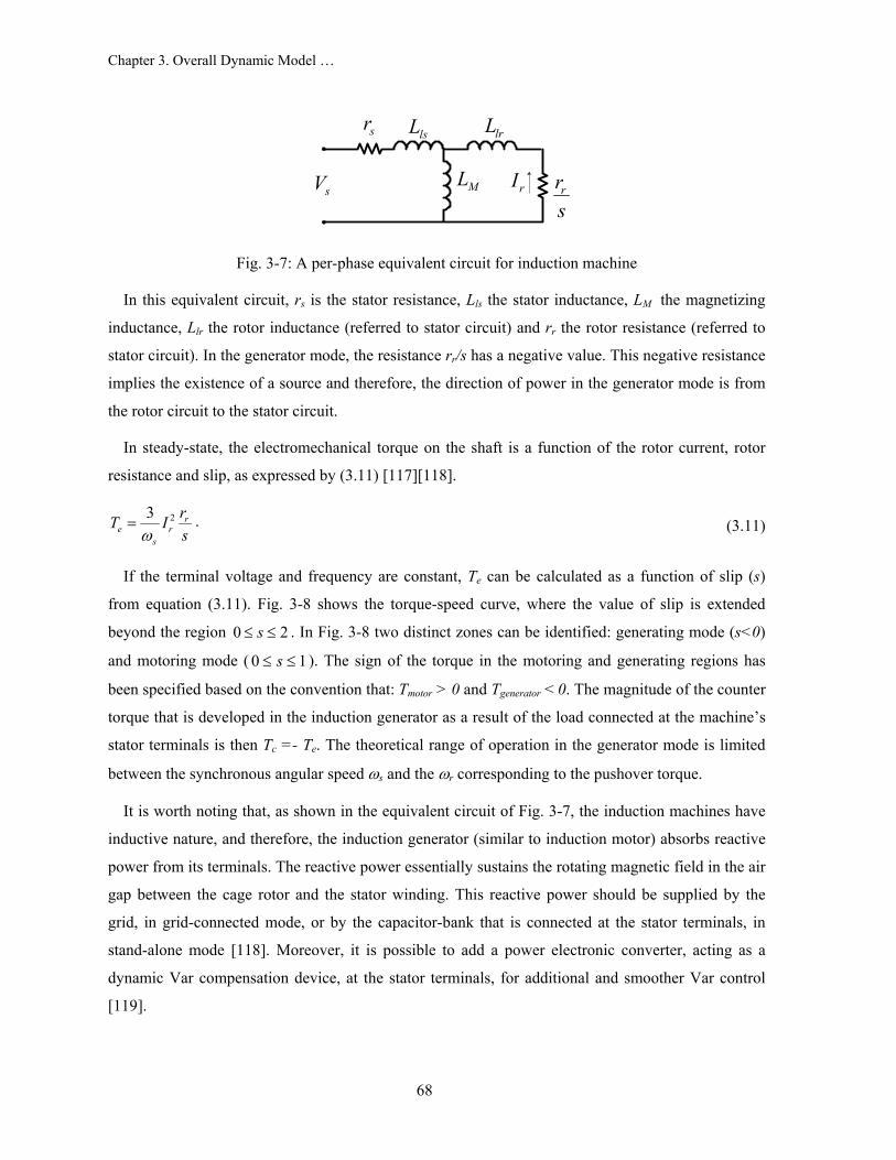
Chapter 3. Overall Dynamic Model …
68
sr lsL
ML
lrL
rrs
sV rI
Fig. 3-7: A per-phase equivalent circuit for induction machine
In this equivalent circuit, rs is the stator resistance, Lls the stator inductance, LM the magnetizing
inductance, Llr the rotor inductance (referred to stator circuit) and rr the rotor resistance (referred to
stator circuit). In the generator mode, the resistance rr/s has a negative value. This negative resistance
implies the existence of a source and therefore, the direction of power in the generator mode is from
the rotor circuit to the stator circuit.
In steady-state, the electromechanical torque on the shaft is a function of the rotor current, rotor
resistance and slip, as expressed by (3.11) [117][118].
23 re r
s
rT Isω
= . (3.11)
If the terminal voltage and frequency are constant, Te can be calculated as a function of slip (s)
from equation (3.11). Fig. 3-8 shows the torque-speed curve, where the value of slip is extended
beyond the region 0 2s≤ ≤ . In Fig. 3-8 two distinct zones can be identified: generating mode (s<0)
and motoring mode ( 0 1s≤ ≤ ). The sign of the torque in the motoring and generating regions has
been specified based on the convention that: Tmotor > 0 and Tgenerator < 0. The magnitude of the counter
torque that is developed in the induction generator as a result of the load connected at the machine’s
stator terminals is then Tc =- Te. The theoretical range of operation in the generator mode is limited
between the synchronous angular speed ωs and the ωr corresponding to the pushover torque.
It is worth noting that, as shown in the equivalent circuit of Fig. 3-7, the induction machines have
inductive nature, and therefore, the induction generator (similar to induction motor) absorbs reactive
power from its terminals. The reactive power essentially sustains the rotating magnetic field in the air
gap between the cage rotor and the stator winding. This reactive power should be supplied by the
grid, in grid-connected mode, or by the capacitor-bank that is connected at the stator terminals, in
stand-alone mode [118]. Moreover, it is possible to add a power electronic converter, acting as a
dynamic Var compensation device, at the stator terminals, for additional and smoother Var control
[119].

Chapter 3. Overall Dynamic Model …
69
The output voltage of the generator, in stand-alone operation, can be estimated from the
intersection point of the magnetization curve of the machine and the impedance line of the capacitor.
This intersection point defines the operating point. Also the output frequency, in a grid connection, is
dictated by the grid, while in stand-alone operation, it is a function of the load, rotor speed and
excitation capacitance [120].
rω rω
M otoring generating
Synchronous Speed
1
0S lip,s
r
s
puωω
Speed
1
0
sω sω
Fig. 3-8: Torque-speed curve of induction machine [117][118]
3.2.3.1 Dynamic Model of the Induction Machine
A commonly-used induction machine model is based on the flux linkages [118]. The dynamic
equivalent circuit of the induction machine in qdo frame is illustrated in Fig. 3-9 [118][121].
sr e dsω Ψ lsL
ML
lsL ( )e re drω ω− Ψ rr
qsi+
-
qrVqri+
-
sr e qsω Ψ lsL
ML
lrL ( )e re qrω ω− Ψ rr
dsi+
-dsV drVdri
+
-
qrqr
b
ϕω
Ψ =qsqs
b
ϕω
Ψ =
dsds
b
ϕω
Ψ = drdr
b
ϕω
Ψ =
qsV
Fig. 3-9: qdo-equivalent circuit of an induction machine [118][121]

Chapter 3. Overall Dynamic Model …
70
Note that in the qdo-equivalent circuit all the rotor parameters are transferred to the stator side. The
machine is described by four differential equations based on flux linkage in the qdo frame and one
differential equation based on rotor electrical angular speed, as follows:
qsbqrdseqsqs vCC
dtd
ωψψωψψ
++−= 21 , (3.12)
dsbdrdsqseds vCC
dtd
ωψψψωψ
+++= 21 , (3.13)
3 4 ( )qrqs qr e re dr
dC C
dtψ
ψ ψ ω ω ψ= + − − , (3.14)
3 4( )drds e re qr dr
d C Cdtψ ψ ω ω ψ ψ= + − + , (3.15)
( )2
ree L
d p T Tdt Jω ⎛ ⎞= −⎜ ⎟
⎝ ⎠, (3.16)
where
)1(*
1 −=ls
ml
ls
sb x
xxrC ω ,
lr
ml
ls
sb x
xxrC
*
2 ω= ,ls
ml
lr
rb x
xxrC
*
3 ω= ,
)1(*
4 −=lr
ml
lr
rb x
xxrC ω , 1111* )( −−−− ++= lrlsmml xxxx ,
dsψ , qsψ , drψ and qrψ : d-axis and q-axis stator and rotor flux linkages,
rr and rs : rotor and stator resistances,
Xls=ωeLls and Xlr=ωeLlr : stator and rotor leakage reactances, Xm=ωeLml : magnetization reactance,
ωe, ωb : stator and base electrical angular speeds, ωre : rotor electrical angular speed,
vqs, vds: q and d-axis stator voltages, vqr, vdr: q and d-axis rotor voltages,
Te and TL: electromechanical and load torque.
The stator and rotor currents, in the qdo-equivalent circuit of Fig. 3-9, can be found as follows:
1 ( )qs qs mqls
ix
ψ ψ= − , (3.17)

Chapter 3. Overall Dynamic Model …
71
1 ( )ds ds mdls
ix
ψ ψ= − , (3.18)
1 ( )qr qr mqlr
ix
ψ ψ= − , (3.19)
1 ( )dr dr mdlr
ix
ψ ψ= − , (3.20)
where
* [ ]qs qrmq ml
ls lr
xx xψ ψ
ψ = + and * [ ]ds drmd ml
ls lr
xx xψ ψψ = + .
In addition, the electromechanical torque of the machine can be written as follows:
53 1 ( ) ( )2 2e ds qs qs ds dr qs qr ds
b
pT i i Cψ ψ ψ ψ ψ ψω
⎛ ⎞= − = −⎜ ⎟⎝ ⎠
, (3.21)
where lrls
ml
b xxxPC
*
51
223
ω= .
3.2.3.2 Constant V/f Speed Control Method
To avoid saturation of induction machine when the stator frequency changes, the stator terminal
voltage is also adjusted using a constant a constant V/f strategy. This method is well known for the
induction machine speed control [122]. A power electronic converter should be employed at the
terminals of the induction generator to implement the constant V/f strategy. In the study reported in
this thesis, this strategy is implemented for adjusting the speed of the turbine shaft to achieve
maximum power point tracking.
3.2.4 Gearbox Model
As mentioned in Chapter 1, the duty of a mechanical gearbox is transforming the mechanical power
from the slow turning rotor shaft to a fast-turning shaft, which drives the generator. The gearbox is
mostly used in the wind turbines with induction generators. The need for this transmission arises
from the problem that an induction generator cannot be built for very low speeds with good
efficiency.

Chapter 3. Overall Dynamic Model …
72
In order to model the gearbox, it is only needed to consider that the generator torque can simply be
transferred to the low speed shaft by a multiplication. For example, for gearbox of Fig. 3-5, one can
write [123]:
gTgear
e T
Tn
Tωω
= = . (3.22)
Note that for a no ideal gearbox, the efficiency of the gearbox should be considered in the model.
3.2.5 Grid model
The grid model consists of an infinite bus. The infinite-bus model can be used when the grid power
capacity is sufficiently large such that the action of any one user or generator will not affect the
operation of the power grid. In an infinite bus, the system frequency and voltage are constant,
independent of active and reactive power flows.
3.2.6 Wind Speed Model
Although the wind model is not part of the wind turbine model, the output power calculation in the
wind turbine rotor requires the knowledge of instantaneous wind speed.
Wind is very difficult to model because of its highly-variable behavior both in location and time.
Wind speed has persistent variations over a long-term scale. However, surface conditions such as
buildings, trees, and areas of water affect the short-term behaviour of the wind and introduce
fluctuations in the flow, i.e., wind speed turbulence.
A brief review of the literature reveals different wind speed models. For example, a wind model
based on superposition of components is proposed in [124]. In this method, the wind speed is
modeled by four components: mean wind speed, ramp wind component, gust wind component and
noise wind component. However, determining all four components is a difficult task.
In this study, wind speed is modeled with a random process. The model is based on Van Der
Hoven and Von Karman’s models [95][125]. The instantaneous value of wind speed, vW (t), can be
described as the wind speed average value plus fluctuations in the wind speed, as follows:
1( ) cos( )
N
W WM i i ii
v t V A tω=
Ψ= + +∑ , (3.23)
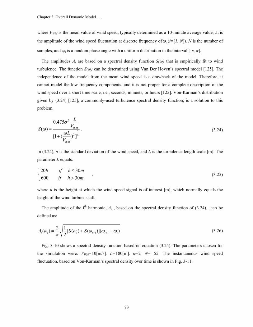
Chapter 3. Overall Dynamic Model …
73
where VWM is the mean value of wind speed, typically determined as a 10-minute average value, Ai is
the amplitude of the wind speed fluctuation at discrete frequency of iω (i=[1, N]), N is the number of
samples, and ψi is a random phase angle with a uniform distribution in the interval [-π, π].
The amplitudes Ai are based on a spectral density function S(ω) that is empirically fit to wind
turbulence. The function S(ω) can be determined using Van Der Hoven’s spectral model [125]. The
independence of the model from the mean wind speed is a drawback of the model. Therefore, it
cannot model the low frequency components, and it is not proper for a complete description of the
wind speed over a short time scale, i.e., seconds, minuets, or hours [125]. Von-Karman’s distribution
given by (3.24) [125], a commonly-used turbulence spectral density function, is a solution to this
problem.
2
52 6
0.475( )
[1 ( ) ]
WM
WM
LVS
LV
σω
ω=
+. (3.24)
In (3.24), σ is the standard deviation of the wind speed, and L is the turbulence length scale [m]. The
parameter L equals:
20 30600 30
h if h mif h m
≤⎧⎨ >⎩
, (3.25)
where h is the height at which the wind speed signal is of interest [m], which normally equals the
height of the wind turbine shaft.
The amplitude of the ith harmonic, Ai , based on the spectral density function of (3.24), can be
defined as:
1 12 1( ) [ ( ) ( )]( )
2i i i i i iA S Sω ω ω ω ωπ + += + − . (3.26)
Fig. 3-10 shows a spectral density function based on equation (3.24). The parameters chosen for
the simulation were: VWM=10[m/s], L=180[m], σ=2, N= 55. The instantaneous wind speed
fluctuation, based on Von-Karman’s spectral density over time is shown in Fig. 3-11.

Chapter 3. Overall Dynamic Model …
74
0 500 1000 1500 2000 2500 3000 3500 40000
0.02
0.04
0.06
0.08
0.1
0.12
0.14
0.16
0.18
fS( ω
)[m2 /s
2 ]
f[Cycles/hour]
Fig. 3-10: Turbulence spectral density function according to Von-Karman’s method
0 5 10 15 20 25 30 35 408
8.5
9
9.5
10
10.5
11
11.5
12
Win
d Sp
eed
[m/s
]
t[Sec]
Fig. 3-11: Instantaneous wind speed as a function of time

Chapter 3. Overall Dynamic Model …
75
3.2.6.1 High-Frequency Damping Effect
For wind power calculations, the instantaneous wind speed model should be augmented with
complex wind effects on the wind turbine blades, including high-frequency damping effects and
tower-shadow effects. In this section, the high-frequency damping effect is discussed.
The phenomenon of damping the high-frequency wind speed variations over the blades surface,
namely high-frequency damping effect, should be included in the aerodynamic model of the wind
turbine [108]. To approximate this effect, a low-pass filter with the following transfer function is
employed.
1( )1
H ssτ
=+
. (3.27)
The filter time constant τ depends on the turbine radius, average wind speed at hub height, and the
intensity of wind turbulence. Fig. 3-12 shows the instantaneous wind speed and corresponding low-
pass filtered signal.
0 5 10 15 20 25 30 35 408
8.5
9
9.5
10
10.5
11
11.5
12Wind Speed
Win
d Sp
eed
[m/s
]
t[Sec]
UnfiltreedLow-pass filtered
Fig. 3-12: Wind speed fluctuation: unfiltered and low pass filtered.
It is worth mentioning that the low-pass filtered wind speed data can be saved in a memory and
used later for simulation, instead of using the instantaneous wind speed data and the low-pass filter
dynamic equation.

Chapter 3. Overall Dynamic Model …
76
3.3 Overall Dynamic Model of the Wind Turbine System
In the previous section and the pervious chapter, the components of the wind turbine system, shown
in Fig. 3-2, were modeled by thirteen nonlinear equations (excluding the wind model): three, given
by equations (3.6)-(3.8), for the wind turbine and shafts; six, given by equation (3.55), for the MC in
balanced three-phase operation; and four, given by (3.17)-(3.20), for the induction machine. Using
these equations, a complete dynamic model of the wind turbine will be developed in this section.
In the proposed system, Fig. 3-1, the input and output sub-circuits of the MC are connected to the
electrical grid and the stator terminals of the induction generator, respectively. Therefore, based on
the quantities defined in Section 3.2 and Chapter 3, the following equations can be written for the
voltages, currents and frequency of the MC, as well as the induction generator terminal voltages:
Generator terminal voltages: _qs q outv v= , _ds d outv v= , (3.28)
Generator terminal currents: qoqs ii = , dods ii = , (3.29)
Generator synchronous frequency and MC input frequency: o eω ω= , i Gridω ω= , (3.30)
MC input sub-circuit terminal voltages: _qG q inv v= , _dG d inv v= . (3.31)
In generator equations (3.12) and (3.13), the generator terminal voltages, vqs and vds, should be
stated in terms of state variables and inputs variables. Note that, for the overall system, the grid
voltage, vqG and vdG, are the input variables.
From equation (2.49) the generator voltage can be written as follows:
_ 0qs q out o qs o qs e ds qodv v L i R i L i vdt
ω= = − − − + , (3.32)
_ds d out o ds o e qs o ds dodv v L i L i R i vdt
ω= = − + − + . (3.33)
Substituting the generator currents, equations (3.17) and (3.18), and their derivations in equations
(3.32) and (3.33), and using equations (3.14) and (3.15), the generator terminal voltages can be
expressed as a function of the system state variables, as follows:

Chapter 3. Overall Dynamic Model …
77
* * * *0
3
* *0
4
( ) [1 ] ( [1 ]) [1 ]
( ) ,
o ml o ml o ml e mlqs qs qs ds
ls ls ls ls ls ls ls ls
ml o o mlqr dr re qo
ls ls ls ls ls
d L x L x R x L xv Cdt x x x x x x x x
x L R L xC vx x x x x
ωψ ψ ψ
ψ ψ ω
−= − + − − − −
+ + + + (3.34)
* * * *
3
* *
4
( ) [1 ] ( [1 ]) ( [1 ])
( ) .
o ml o e ml o ml o mlds ds qs ds
ls ls ls ls ls ls ls ls
o ml mlqr re dr o o do
ls ls ls ls
d L x L x L x R xv Cdt x x x x x x x x
L x x L C R vx x x x
ωψ ψ ψ
ψ ω ψ
−= − + − + − −
− + + + (3.35)
Next, using equations (3.34) and (3.35), the stator flux linkage equations, (3.12) and (3.13), can be
presented as a function of system state variables, as follows:
* * * * *1 2 3 4 5qs qs e ds qr dr re qo
d C C C C C vdtψ ψ ωψ ψ ψ ω= + + + + , (3.36)
* * * * *2 1 4 3 5ds e qs ds qr re dr do
d C C C C C vdtψ ωψ ψ ψ ω ψ= − + − + + , (3.37)
where
1]1[*
0 +−=ls
ml
ls
ob x
xxLC ω , ])1[(1 **
310
*1
ls
ml
ls
ob
ls
ml
ls
ob
xx
xR
xx
xLCC
CC −−+=
ωω,
** 02
0
1 ( 1 [1 ])b ml
ls ls
L xCC x x
ω= − − − , ))((1
4
*
20
*3
ls
o
ls
o
ls
mlb
xR
xLC
xxC
CC ++=
ω,
ls
ml
ls
b
xx
xL
CC
*0
0
*4
1 ω= , *
50
1CC
= .
Finally, by combining the state-equation of the mechanical shaft, electrical generator, and the MC,
the overall model of the system can be described by the following eleven nonlinear equations. The
derivation of the overall system model from the component’s models and all the constant coefficients
has been presented in Appendix G.
1 12 1
gridD D D DiqG qG dG qo qG
i i i
Rd i i i v vdt L a L L
ω= − − − +
−, (3.38)
1 1(2 1)D D D DidG grid qG dG do dG
i i i
Rd i a i i v vdt L L L
ω= − − − + , (3.39)

Chapter 3. Overall Dynamic Model …
78
7 7 8 81
2 1gridD
qo qs ds qr dr qG dod v A A A A i vdt C a
ωϕ ϕ ϕ ϕ′ ′= + + + + −
−, (3.40)
2 2 2 27 7 8 8(2 1) (2 1) (2 1) (2 1)
1 (2 1) ,
do qs ds qr dr
DdG grid qo
d v A a A a A a A adt
i a vC
ϕ ϕ ϕ ϕ
ω
′ ′= − + − + − + −
+ + − (3.41)
* * * * *1 2 3 4 5qs qs e ds qr dr g e qo
d C C C C C vdtψ ψ ωψ ψ ψ ω ω= + + + + , (3.42)
* * * * *2 1 4 3 5ds e qs ds qr g dr e do
d C C C C C vdtψ ωψ ψ ψ ω ψ ω= − + − + + , (3.43)
3 4 ( )qr qs qr e g drd C Cdtψ ψ ψ ω ω ψ= + − − , (3.44)
3 4( )dr ds e g qr drd C Cdtψ ψ ω ω ψ ψ= + − + , (3.45)
5
21 1[ ( ( ) ( )]gG s T dr qs qr ds
G gear gear
d K B Cdt J n P n
ωω θ ω ψ ψ ψ ψ= ∆ + − − − , (3.46)
2 gT
gear
ddt P n
ωθ ω= − , (3.47)
3 21 1[ ( , ) ( ( )]2
gT r p w s T
T T G
d A C V K Bdt J PR
ωω ρ β λ θ ω
ω= − ∆ + − . (3.48)
The power exchanged between grid and the wind turbine is an important quantity of the wind
turbine system. Therefore, the grid active and reactive powers injected into the grid are chosen as the
output variables for the model. The formula for the grid power based on the equations (2.73) and
(2.75) can be written as follows:
3 [cos( ) sin( ) ]
2D D
Grid Gm o qG o dGP V i iq
α α= − , (3.49)
3 (sin( ) cos( ) )2 2 1
D DGmGrid o qG o dG
VQ i iq a
α α=− +−
, (3.50)
where VGm is the peak value of the grid phase voltage.
The schematic diagram of the wind turbine system’s overall dynamic model is shown in Fig. 3-13.
The model is characterized by six inputs u , two outputs y , and eleven state variables x . Out of the
six inputs, ωe, q, a, and αo are adjustable control variables of the MC, β is pitch angle of the turbine

Chapter 3. Overall Dynamic Model …
79
blades, and VW is the wind velocity. The active and reactive powers injected into the grid are treated
as output variables for the model.
DqGiDdGiqovdov
qsψdsψqrψdrψ
gωδθ
Tω
eω
q
a
oα
WV
β
GridP
GridQ
Inputs States Outputs yxu
MC Output frequency
MC Voltage gain
DPF control
MC voltage angle
Wind vlocity
Pitch angle
Fig. 3-13 Inputs, state variables and outputs of the overall dynamic model of wind turbine system
3.4 Verification of the Overall Dynamic Model
Here, the objective is to study the behavior of the system output variables, i.e., active and reactive
powers injected into the utility grid, in response to variations of the input variables. In the following
subsections, first the starting operation of the system will be simulated. Then, steady-state
performance of the system for some input variations is investigated. Finally, the dynamic behavior of
the model will be investigated by simulating its step responses. Although the realistic wind speed
model was described in section 3.2.6, without loss of generality, in the following simulations the
wind velocity is considered as a constant signal.
3.4.1 Starting the Wind Turbine System
The soft-starting procedure to reduce inrush current during the connection of the wind turbine to the
grid was discussed in Chapter 1. This subsection, the system simulation starts with the wind turbine
already connected to the grid [126]. The parameters of the wind turbine system are shown in
Appendix L (Table L.2).
Fig. 3-14 shows the active and reactive power injected into the grid. The simulation starts with
zero shaft speed and rated grid voltage. The electrical machine initially works in the motoring mode

Chapter 3. Overall Dynamic Model …
80
and draws active power from the grid. When the shaft speeds up and the wind power increases, the
machine switches to the generating mode and the direction of the power-flow will be changed from
the generator to the grid. Table 3.2 shows the values for the model input parameters, the grid power,
and the power factor at the operating point. The base values for the grid power and voltage are
Sb=100 [kVA] and Vbll
(rms)=4 [kV], respectively. Also, the phase-a and zoomed-in three-phase grid
currents during the starting and steady-state operation are shown in Fig. 3-15.
0 0.1 0.2 0.3 0.4 0.5 0.6 0.7 0.8 0.9-1000
-500
0
500Power Injected to the Grid
Act
ive
Pow
er [k
W]
time[sec]
0 0.1 0.2 0.3 0.4 0.5 0.6 0.7 0.8 0.90
500
1000
Reac
tive
Pow
er[k
Var]
time[sec]
Fig. 3-14: Grid active and reactive power during the starting and the steady-state operation.
Table 3.2: Values of the input parameters and the grid power at the operating point
Voltage
Gain
Output
voltage
angle
MC output
frequency
Pitch
Angle
DPF
Control Wind Speed
Grid Power and
power factor
q=0.5 αο=0 fe = 6o [Hz] β=0 a=0.8 VW=10[m/s]
PGrid= 82.76[kW]
QGrid=40.87[kVar]
PFGrid=0.89

Chapter 3. Overall Dynamic Model …
81
0 0.1 0.2 0.3 0.4 0.5 0.6 0.7-200
-100
0
100
200One-phase grid current
[Am
p.]
time[sec]
0.7 0.72 0.74 0.76 0.78 0.8 0.82 0.84 0.86 0.88 0.9
-20
-10
0
10
20
Zoomed in three-phase grid currents
[Am
p.]
time[sec]
Fig. 3-15: Phase-a and three-phase grid current during the starting and steady-state operation.
3.4.2 Steady-State Performance of the System
The active and reactive powers injected into the grid are functions of the system inputs. Therefore, it
is important to know how the grid power varies as the inputs of the system vary in their permitted
ranges. In the following, the system steady-state output response to variations of the MC output
frequency, voltage gain, and output voltage angle, as well as, parameter ‘a’, are discussed.
Fig. 3-16 shows the steady-state grid active and reactive powers versus the MC output frequency,
while other inputs of the system remain fixed at the rated values based on Table 3.1. As shown in Fig.
3-16, the active power first increases and then decreases as the frequency rises, while the reactive
power decreases. The behavior of the active power verses frequency variation can be explained based
on the wind turbine’s power-verses-speed curve and the electrical generator power-verses-frequency
curve, which will be are discussed further detail in Chapter 5 [95]. In addition, increasing the MC
output frequency raises the consumption of the system reactive power, hence the reactive power
injected to the grid will be decreased.
Fig. 3-17 shows the steady-state grid active and reactive power versus the MC gain voltage. The
gain voltage variation has a significant effect on the grid reactive power and a minor effect on the
grid active power [95].

Chapter 3. Overall Dynamic Model …
82
0.7 0.8 0.9 1 1.1 1.2 1.3 1.4 1.5 1.60.5
0.6
0.7
0.8
0.9Grid Active and Reactive Power
P[p
.u.]
0.7 0.8 0.9 1 1.1 1.2 1.3 1.4 1.5 1.60.2
0.3
0.4
0.5
0.6
0.7
Q[p
.u.]
MC Output frequency [p.u.]
Fig. 3-16: Steady-state grid active and reactive power versus the MC output frequency
0.6 0.8 1 1.2 1.4 1.6 1.80.8
0.81
0.82
0.83
Grid Active and Reactive Power
P[p
.u.]
0.6 0.8 1 1.2 1.4 1.6 1.80
0.5
1
1.5
Q[p
.u.]
MC voltage gain [p.u.]
Fig. 3-17: Steady-state grid active and reactive powers versus the MC voltage gain

Chapter 3. Overall Dynamic Model …
83
Fig. 3-18 shows linear variations in grid reactive power in both lagging and leading regions,
corresponding to the ranges, 0%a<0.5 and 0.5<a%1, respectively. Note that the grid active power
(not shown) is almost constant for variations of parameter ‘a’.
Fig. 3-19 shows the system outputs versus the MC output voltage angle, αo. Both grid active and
reactive powers change dramatically with the angle αo. The electrical machine enters motoring mode,
P<0, for some ranges of variations of the MC output voltage angle. The results show that αo is not an
appropriate input to control the system, because it causes severe variations in the system outputs and
sometimes makes the machine swing between generatoring and motoring modes. Therefore, the MC
output voltage angle will be kept constant at αo =0 in the rest of this thesis to maintain the machine in
the generatoring mode.
0.2 0.3 0.4 0.5 0.6 0.7 0.80.1
0.15
0.2
0.25
0.3
0.35
0.4
0.45
0.5
0.55
0.6Grid Reactive Power
Q[p
.u.]
Parameter " a"
LeadingLagging
Fig. 3-18: Steady-state grid reactive power versus the parameter ‘a’ in lagging and leading regions.
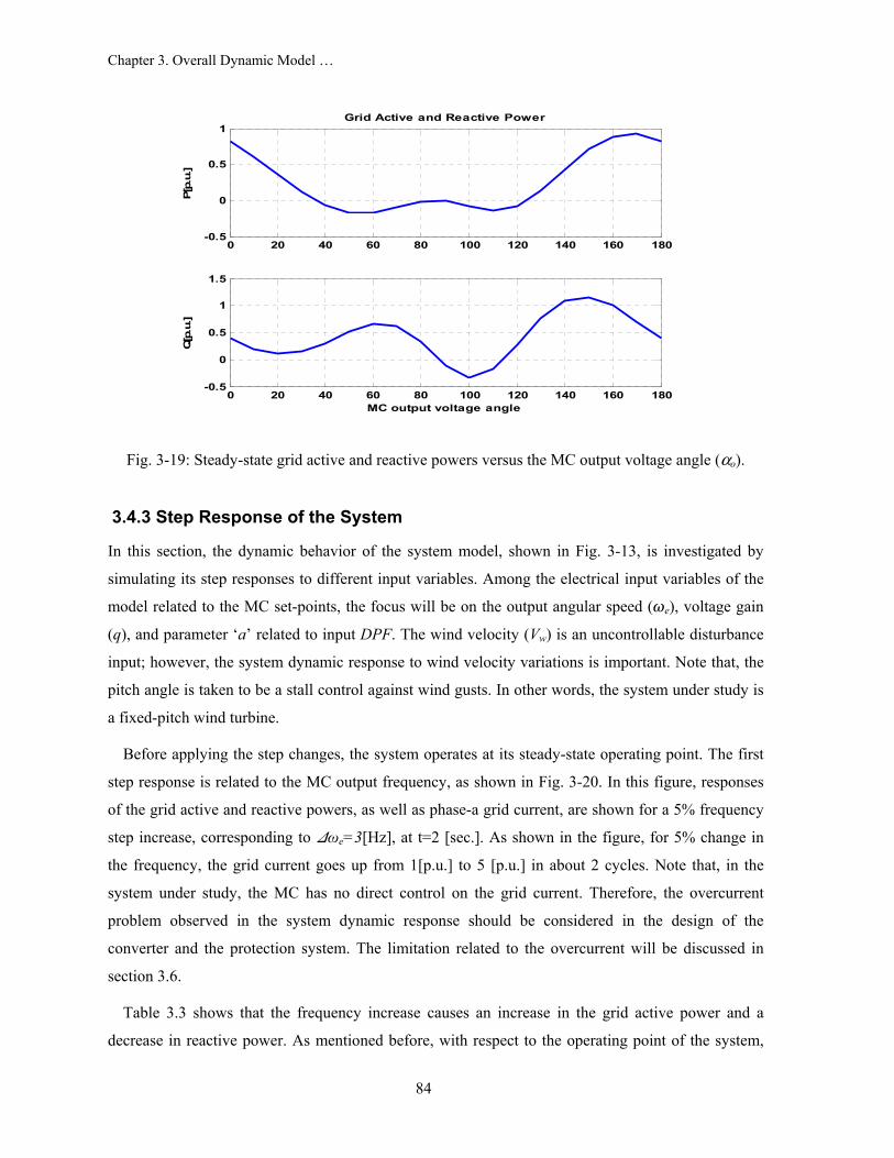
Chapter 3. Overall Dynamic Model …
84
0 20 40 60 80 100 120 140 160 180-0.5
0
0.5
1Grid Active and Reactive Power
P[p
.u.]
0 20 40 60 80 100 120 140 160 180-0.5
0
0.5
1
1.5
Q[p
.u.]
MC output voltage angle
Fig. 3-19: Steady-state grid active and reactive powers versus the MC output voltage angle (αo).
3.4.3 Step Response of the System
In this section, the dynamic behavior of the system model, shown in Fig. 3-13, is investigated by
simulating its step responses to different input variables. Among the electrical input variables of the
model related to the MC set-points, the focus will be on the output angular speed (ωe), voltage gain
(q), and parameter ‘a’ related to input DPF. The wind velocity (Vw) is an uncontrollable disturbance
input; however, the system dynamic response to wind velocity variations is important. Note that, the
pitch angle is taken to be a stall control against wind gusts. In other words, the system under study is
a fixed-pitch wind turbine.
Before applying the step changes, the system operates at its steady-state operating point. The first
step response is related to the MC output frequency, as shown in Fig. 3-20. In this figure, responses
of the grid active and reactive powers, as well as phase-a grid current, are shown for a 5% frequency
step increase, corresponding to Dωe=3[Hz], at t=2 [sec.]. As shown in the figure, for 5% change in
the frequency, the grid current goes up from 1[p.u.] to 5 [p.u.] in about 2 cycles. Note that, in the
system under study, the MC has no direct control on the grid current. Therefore, the overcurrent
problem observed in the system dynamic response should be considered in the design of the
converter and the protection system. The limitation related to the overcurrent will be discussed in
section 3.6.
Table 3.3 shows that the frequency increase causes an increase in the grid active power and a
decrease in reactive power. As mentioned before, with respect to the operating point of the system,

Chapter 3. Overall Dynamic Model …
85
increasing the frequency may increase or decrease the active power. However, in this case, the
frequency increase causes the increase in consumption of the system reactive power. Note that, from
the control point of view, the system response to a step change in frequency indicates that the system
is of non-minimum-phase nature.
0.1 0.2 0.3 0.4 0.5 0.6 0.7-4
-20
2Grid Active Power
[p.u
.]
0.1 0.2 0.3 0.4 0.5 0.6 0.70.2
0.4
0.6
Grid Reactive Power
[p.u
.]
0.1 0.2 0.3 0.4 0.5 0.6 0.7-5
0
5phase-a Grid Current
[p.u
.]
time[Sec]
Fig. 3-20: Grid active and reactive powers and phase-a grid current responses of the dynamic wind
model to 5% step increase in the MC output frequency (ωe) at t=0.2[sec.].
Fig. 3-21 shows the step response of the system to a 5% step increase in the MC voltage gain (q).
As shown in this figure and Table 3.3, voltage gain increase results in a significant increase in grid
reactive power, while active power remains almost constant, because reactive power, unlike active
power, is highly dependent on the voltage magnitude.
A big step change is considered for the parameter “a”, related to grid DPF control, as shown in Fig.
3-22. The step response of Fig. 3-22 and results in Table 3.3 reveal that the system is stable with this
big step change, and also that grid reactive power is changed from the leading to the lagging state.
This big change in the parameter “a” is applied to the system to show the capability of the system
reactive power control.
Finally, the last step response is related to the wind velocity. As mentioned earlier, the wind
velocity is an uncontrollable input and its step change shows the system performance for disturbance
variation. The step response, illustrated in Fig. 3-23, and the results in Table 3.3, show that wind

Chapter 3. Overall Dynamic Model …
86
velocity increments dramatically increase the grid active power. This occurs because of increase in
the turbine mechanical power.
0.1 0.15 0.2 0.25 0.3 0.35 0.4 0.45 0.50.20.40.60.8
11.2
Grid Active Power[p
.u.]
0.1 0.15 0.2 0.25 0.3 0.35 0.4 0.45 0.5
0.5
1
Grid Reactive Power
[p.u
.]
0.1 0.15 0.2 0.25 0.3 0.35 0.4 0.45 0.5
-101
Phase-a Grid Current
[p.u
.]
time[sec]
Fig. 3-21: Grid active and reactive powers and phase-a grid current responses of the dynamic wind
model to 10% step increase in the MC voltage gain at t=0.2[sec.]
0.1 0.15 0.2 0.25 0.3 0.35 0.4 0.45 0.5
0.70.80.9
Grid Active Power
[p.u
.]
0.1 0.15 0.2 0.25 0.3 0.35 0.4 0.45 0.5
-0.5
0
0.5Grid Reactive Power
[p.u
.]
0.1 0.15 0.2 0.25 0.3 0.35 0.4 0.45 0.5
-1
0
1
Phase-a Grid Current
[p.u
.]
time[sec]
Fig. 3-22: Grid active and reactive powers and phase-a grid current responses of the dynamic wind
model to 75% step decrease in the parameter “a” at t=0.2[sec]

Chapter 3. Overall Dynamic Model …
87
0.1 0.15 0.2 0.25 0.3 0.35 0.4 0.45 0.50.8
1
Grid Active Power
[p.u
.]
0.1 0.15 0.2 0.25 0.3 0.35 0.4 0.45 0.50.4
0.42
0.44Grid Reactive Power
[p.u
.]
0.1 0.15 0.2 0.25 0.3 0.35 0.4 0.45 0.5-2
0
2Phase-a Grid Current
[p.u
.]
time[sec]
Fig. 3-23: Grid active and reactive powers and phase-a grid current responses of the dynamic wind
model to 10% step increase in the wind velocity at t=0.2[sec.].
Table 3.3: Variations in output variables of the wind turbine model against some input variations
ef∆ =5% q∆ =5% a∆ =-75% WV∆ =10%
GridP∆ 1.82% 0.09% 0.05% 25.56%
GridQ∆ -4.4% 10.12% -229.5% 4.82%
3.5 Overall Dynamic Model and Constant V/f Strategy
As mentioned in Subsection 3.2.3.2, the terminal voltage and frequency of the induction generator are
usually controlled according to the constant V/f strategy to avoid flux saturation. The ratio of the
variation of voltage and frequency is:
_
ratedVF
e rated
qKω
= , (3.51)
where KVF is a constant parameter, and qrated and ωe_rated are the MC rated voltage gain and output
frequency, respectively.

Chapter 3. Overall Dynamic Model …
88
To take into account the constant V/f strategy in the overall dynamic model, shown in Fig. 3-13,
the model should be modified based on the equation (3.51). The modified model nonlinear dynamic
equations are given in Appendix H.
3.5.1 Verification of the Overall Dynamic Model with Constant V/f Strategy
The steady-state and dynamic behaviors of the model with constant V/f strategy for the input
variations must be the same as the results shown in the previous section, except for the MC frequency
output. Therefore, the output response of the new model is verified only for the MC frequency
change. Because of the constant V/f strategy, a change in the frequency is proportional to a change in
the MC voltage gain whose magnitude can be determined based on the equation (3.51).
Fig. 3-24 shows the steady-state grid active and reactive powers verses the MC output frequency.
During frequency increase, grid active power increases and then decreases, while reactive power
increases with an almost constant slope. Increasing the frequency corresponds to increase in the
voltage gain and the resulting increase in reactive power.
0.7 0.8 0.9 1 1.1 1.2 1.3 1.4 1.5 1.6
0.5
0.6
0.7
0.8
Grid Active and Reactive Power
P[p
.u.]
0.7 0.8 0.9 1 1.1 1.2 1.3 1.4 1.5 1.60.2
0.3
0.4
0.5
0.6
0.7
Q[p
.u.]
MC Output frequency [p.u.]
Fig. 3-24: Steady-state grid active and reactive powers versus the MC output frequency with constant
V/f strategy
For the dynamic response, consistent with the previous simulation, a 5% step-increase is applied at
t=2 [sec.] to the MC set-point frequency. Fig. 3-25 illustrates the step response of the grid power and

Chapter 3. Overall Dynamic Model …
89
phase-a current. In addition, Table 3.4 shows the steady-state changes of the grid active and reactive
powers for the applied step change.
The dynamic and steady-state results, Fig. 3-25 and Table 3.4, can be interpreted by considering
the results of step change in frequency and the voltage gain, Fig. 3-20, Fig. 3-21 and Table 3.3, and
coupling effects between the grid active and reactive power. As a result, changes in frequency affect
both active and reactive power, but the magnitude of these effects depends on to the system operating
point.
0.1 0.2 0.3 0.4 0.5 0.6 0.7-4
-20
2Grid Active Power
[p.u
.]
0.1 0.2 0.3 0.4 0.5 0.6 0.7
0.5
1Grid Reactive Power
[p.u
.]
0.1 0.2 0.3 0.4 0.5 0.6 0.7-5
0
5Phase-a Grid Current
[p.u
.]
time[sec]
Fig. 3-25: Grid active and reactive powers and phase-a grid current responses of the dynamic wind
model with constant V/f strategy to 5% step-increase in the MC output frequency at t=0.2[sec.]
Table 3.4: Variations of output variables of the wind turbine model with constant V/f strategy for step
change in frequency and voltage gain
ef∆ =5%
GridP∆ 1.82%
GridQ∆ 5.12%

Chapter 3. Overall Dynamic Model …
90
3.6 Limitations of the variables changes
The allowable range of variation of system variables are determined by the ratings of system
components. As shown in Figs. 3-20 and 3-25, in response to a small step change in the generator
terminal frequency in the open-loop system, the grid current rises from 1 [p.u.] to 5 [p.u.] over 2
cycles. Devices such as MC switches cannot tolerate currents of five times their rated values in
transients lasting 2 cycles. Sizing the devices based on the maximum transient current is not
economical either. In actual wind turbine systems, such large over-currents can be avoided by
applying changes in the control variables in the form of a ramp function instead of a step function. In
the closed-loop system, there are no step changes in the wind velocity (Fig. 3-12), and as a result, no
step changes in the control variables occur.
Fig. 3-26 shows a 5% ramp-increase in the MC frequency at t=0.2 [sec]. Comparing the grid
current in this figure with that in Fig. 3-25 shows that the maximum transient current has been limited
to 1.6 [p.u.]. This allows for sizing the system component more economically. Note that there are no
limitations in using step-change for other inputs. For example, in Fig. 3-22 a step-change in the
parameter a results in no significant transient current.
0.1 0.2 0.3 0.4 0.5 0.6 0.71
1.02
1.04
1.06Ramp input
[p.u
.]
0.1 0.2 0.3 0.4 0.5 0.6 0.7-2
-1
0
1
2Phase-a Grid Current
[p.u
.]
time[sec]
Fig. 3-26: Phase-a grid current response of the dynamic model with constant V/f strategy to a 5%
ramp-increase in the MC output frequency at t=0.2 [sec].

Chapter 3. Overall Dynamic Model …
91
3.7 Linearized Model of the Wind Turbine System
The nonlinear state-space model of the wind turbine system (with constant V/f strategy) presented in
section 3.5, contains eleven nonlinear equations. The sources of nonlinearity are the turbine torque
equation (3.2), induction machine equations (3.12)-(3.16), and the MC equation (2.58).
In the next sections, a small-signal model is used to systematically study local stability,
controllability, and observability. The small-signal model is developed by linearizing the eleven
nonlinear equations (Appendix H) around an operating point. The linearized model, is described by
the following state-space equations:
dX A X B U
dt∆ = ∆ + ∆ ,
Y C X D U∆ = ∆ + ∆ ,
(3.52)
where
[ ( ) ]D D TqG dG qo do qs ds qr dr g TX i i v v ω δθ ω∆ = ∆ ∆ ∆ ∆ ∆Ψ ∆Ψ ∆Ψ ∆Ψ ∆ ∆ ∆ ,
[ ]Te o WU q a Vω α β∆∆ = ∆ ∆ ∆ ∆ ∆ , and [ ]Grid Grid
TY P Q∆ = ∆ ∆ .
In equation (3.52), A, B, C, and D are the Jacobian matrices, calculated at the operating point. The
detailed linearization of the nonlinear equations is presented in Appendix I. This linearization results
in the matrices A, B, C, and D as follows:
0
0
3,5 3,6 3,7 3,80
04,5 4,6 4,7 4,8
* 0 * * 0 * * 0 * 05 1 2 3 4 4
* 0 * 0 * * 0 * *5 2 1 4 3 4
1 0 0 0 0 0 0 0 02 1
1(2 1) 0 0 0 0 0 0 0 0
1 0 0 0 0 02 1
10 (2 1) 0 0 0 0
0 0 0 0 00 0 0
grid
girdi
i i
i
i i
grid
grid
e e g dr
e e g qr
RL a L
RaL L
a a a aC a
a a a a aC
C C C C C CAC C C C C C
ω
ω
ω
ω
ω ω ω ϕω ω ω ϕ
− − −−
− − −
−−
−
=− − − 0
0 0 03 4
0 0 03 4
9,5 9,6 9,7 9,8 2
7 5 11,11
0 00 0 0 0 0 0 00 0 0 0 0 0 0
20 0 0 0
20 0 0 0 0 0 0 0 0 1
0 0 0 0 0 0 0 0
g e dr
e g qr
s
G gear G gear G gear
gear
C CC C
B K Ba a a aPJ n J n J n
Pn
K K a
ω ω ϕω ω ϕ
⎡ ⎤⎢ ⎥⎢ ⎥⎢ ⎥⎢ ⎥⎢ ⎥⎢ ⎥⎢ ⎥⎢ ⎥⎢ ⎥⎢ ⎥⎢ ⎥⎢ ⎥⎢ ⎥⎢ ⎥⎢ ⎥−⎢ ⎥
− −⎢ ⎥⎢ ⎥
−⎢ ⎥⎢ ⎥⎢ ⎥⎢ ⎥−⎢ ⎥⎢ ⎥⎣ ⎦

Chapter 3. Overall Dynamic Model …
92
0 00
2
0 00
0
3,1 3,30 2
4,1 4,2 4,3* 0 * 02 5
* 0 * 02 5
0
cos( ) 2 (sin( ) )( ) 0 0(2 1)
sin( ) (cos( ) )2 ( ) 0 0
20 0
(2 1)0 0
0 0 0 0
0 0 0 00 0 0 0
DM VF o i dG M VF o e
i i
DM VF o M VF o egrid qG
i i
grid do
ds qo
qs do
dr
qr
V K i V KL a L
V K V Ki
L L
vb b
ab b b
BC C v
C C v
α ω α ω
α α ωω
ω
ψ
ψ
ψ
ψ
−−
− −
−
=+
− +
−0
9,1
11,4 11,5
0 0 0 00 0 0 0
0 0 0 0 00 0 0
b
b b
⎡ ⎤⎢ ⎥⎢ ⎥⎢ ⎥⎢ ⎥⎢ ⎥⎢ ⎥⎢ ⎥⎢ ⎥⎢ ⎥⎢ ⎥⎢ ⎥⎢ ⎥⎢ ⎥⎢ ⎥⎢ ⎥⎢ ⎥⎢ ⎥⎢ ⎥⎢ ⎥⎢ ⎥⎣ ⎦
,
0 0
0 0 0
cos sin 0 0 0 0 0 0 0 0 03
sin cos2 ( ) ( ) 0 0 0 0 0 0 0 0 02 1 2 1
o oGm
o oVF e
VC
Ka a
α α
α αω
−= − −
− −
⎡ ⎤⎢ ⎥⎢ ⎥⎢ ⎥⎣ ⎦
,
0 0
00 0 0
2
cos sin( ) 0 ( sin cos ) 0 0
32 sin cos sin cos cos( ) sin( )
( ) 2( ) ( ) 0 0(2 1) (2 1) 2 1
D DqG o dG o D D
qG o dG oeGm
D D D D D DVF e qG o dG o qG o dG o o qG o dG
e
i ii i
VDK i i i i i i
a a a
α αα α
ωω α α α α α α
ω
⎡ ⎤−+⎢ ⎥
⎢ ⎥= − ⎢ ⎥+ + −⎢ ⎥− −− − −⎢ ⎥⎣ ⎦
.
The constant parameters in the above matrices are given in Appendix I. Also, the superscript "0”
indicates the variable value at the operating point.
The small-signal model of the wind turbine system is illustrated schematically in Fig. 3-27.
eω∆q∆a∆
oα∆
WV∆β∆
GridP∆
GridQ∆
Linearized Model
d X A X B Udt
∆ = ∆ + ∆
Y C X D U∆ = ∆ + ∆
U∆ Y∆X∆
Fig. 3-27: Small-signal model of the wind turbine system

Chapter 3. Overall Dynamic Model …
93
3.8 Linearized Model Performance Evaluation
In order to evaluate the linearization error at an operating point, the linearized model responses to
step changes in some inputs are compared with those of the nonlinear model.
The numerical values in the Jacobian matrices A, B, C, and D at the operating point are shown in
Appendix I. The operating point is given in Table 3.5.
Table 3.5: Input, state and output variables at the operating point for linearization
0 2 60[ / s]e radω π= 0 0.5q = 0 0.8a = 0 0o
α = 0 10[ / ]W
V m s=
0 0β = 0( ) 8.45[ ]DqGi A= − 0( ) 2.5[ ]D
dGi A= 0 1632.3[ ]qo
v V= 0 2.16[ ]do
v V= −
0 26.45[ ]qs
WbΨ = 0 1632.5[ ]ds
WbΨ = 0 109.5[ ]qr
WbΨ = 0 1591.1[ ]dr
WbΨ = 0 378.5[ / ]g
rad sω =
0 0.004[ ]radδθ = 0 9.45[ ]T
radω = 0 82.79[ ]GridP kW= 0 40.88[ ]GridQ kW=
Fig. 3-28 shows the system response to a step increase of 1 Hz (6.28 rad/sec) in the MC output
frequency for linearized and nonlinear models. In the next simulation, the system response to a 10%
step change in parameter ‘a’ for linearized and nonlinear models is obtained (see Fig. 3-29). Fig. 3-30
provides the response of the system to a 5% step increase in wind velocity for linearized and
nonlinear models.
0 0.1 0.2 0.3 0.4 0.5 0.6 0.7 0.8-1
0
1
2Step Response of the Grid Active Power for ∆ωe=6.2832 [rad/sec.]
P [p
.u.]
Nonlinear ModelLinear Model
0 0.1 0.2 0.3 0.4 0.5 0.6 0.7 0.80.2
0.4
0.6
0.8Step Response of the Grid Reactive Power for ∆ωe=6.2832[rad/sec.]
t[sec]
Q [p
.u.]
Fig. 3-28: System response to a step change in the MC output frequency with nonlinear and
linearized models

Chapter 3. Overall Dynamic Model …
94
0.08 0.1 0.12 0.14 0.16 0.18 0.2 0.22 0.24
0.7
0.8
0.9
1Step Response of the Grid Active Power for ∆a=10%
P [p
.u.]
0.08 0.1 0.12 0.14 0.16 0.18 0.20.2
0.4
0.6
0.8
1Step Response of the Grid Reactive Power for ∆a=10%
t[Sec]
Q [p
.u.]
Nonlinear ModelLinear Model
(a)
0.1 0.101 0.102 0.103 0.104 0.105 0.106
0.7
0.8
0.9
1Step Response of the Grid Active Power for ∆a=10%
P [p
.u.]
0.1 0.101 0.102 0.103 0.104 0.105 0.106
0.3
0.4
0.5
0.6
0.7
Step Response of the Grid Reactive Power for ∆a=10%
t[sec]
Q [p
.u.]
Nonlinear ModelLinear Model
(b)
Fig. 3-29: System response to a step change in parameter a of the MC with nonlinear and linear
models, (a) Zoomed out view (b) Zoomed in view

Chapter 3. Overall Dynamic Model …
95
0 0.1 0.2 0.3 0.4 0.5 0.6
0.85
0.9
0.95
Step Response of the Grid Active Power for ∆ VW=5%
P [p
.u.] Nonlinear Model
Linear Model
0 0.1 0.2 0.3 0.4 0.5 0.60.4
0.405
0.41
0.415
0.42
Step Response of the Grid Reactive Power for ∆ VW=5%
t[Sec]
Q [p
.u.]
Fig. 3-30: System response to a step change in the wind velocity with nonlinear and linear models
The simulation results reveal that the small-signal linear model is an accurate approximation of the
nonlinear model.
3.9 Local Stability Evaluation
Different methods to verify the local stability are pointed out in the literature [127][128]. A common
method is to check the eigenvalues of the linearized system. When the real parts of all eigenvalues of
the linearized system are negative, the nonlinear system is locally stable around the steady-state
operating point [129] .
The eigenvalues of the small-signal model linearized around the operating point (Table 3.5) are
shown in Table 3.6. The real parts of all eigenvalues are negative; therefore, the linearized small-
signal model is asymptotically stable at the steady-state operating point.
Table 3.6 Eigenvalues of the linearized system at the operating point
Eigenvalues
-12.205 ± 32.232i
-25.237
-28.126 ± 140.2i
-49.646 ± 32400i
-49.764 ± 31574i
-50.91± 372.8i

Chapter 3. Overall Dynamic Model …
96
3.10 Controllability and Observability Controllability and obeservability are important properties of a system to be controlled. The
fundamental controllability issue is associated with the question of whether the system states can be
controlled in a time interval with a bounded input. Observability describes the ability to determine the
system states with output measurements in a time interval.
The well-known theoretical method for testing controllability/observability is to check if the
controllability /observability matrix has a full rank. This technique is normally not appropriate for
numerical reasons.
3.10.1 Gramian method
One alternative method for testing controllability and observability of continuous and linear-time-
invariant systems starts with solving the Lyapunov equation [127]
TTCC BBAWAW −=+ , (3.53)
where Wc is named controllability Gramian.
Similarly, to test observability, the observability Gramian Wo is computed as
CCAWWA Too
T −=+ . (3.54)
The system is controllable and observable if Wc and Wo are full-rank matrices.
In order to check the rank of the matrices, the singular value decomposition (SVD) method can be
applied. Based on the SVD theorem, every n×p matrix X can be decomposed into a product of three
matrices R, S, and Q, so that [127][130]
TRSQX = , (3.55)
where 1( ,..., ) n nnR r r ×= ∈ℜ and 1( ,..., ) p p
pQ q q ×= ∈ℜ are orthogonal matrices,
1( ,..., ) n pqS diag σ σ ×= ∈ℜ , and 0...21 ≥≥≥≥ qσσσ ( min( , )q n p= ) are singular values of matrix X.
In the linearized model of the system, the SVD of Wc and Wo at the operating point are shown in
Table 3.7. Based on Table 3.7, all singular values of the matrices Wc and Wo are non-zero, and
therefore, the system is completely controllable and observable. However, the singular values of Wc
and Wo are distributed in wide ranges, the evidence of an ill-conditioned system. To show this fact, an
index called condition-number can be used. The condition number is defined as

Chapter 3. Overall Dynamic Model …
97
Condition number = σmax / σmin .
The condition number reveals the size of the numerical error that is likely to be introduced by
matrix computations. While a large condition number denotes an ill-conditioned system, a number
close to one indicates a well-conditioned system. For example, the condition-number for the singular
values of Wc is 2.0913×10¹⁶; therefore, this large number implies the matrix is ill-conditioned and
close to rank deficiency.
3.11 Balanced Realization
This section is dedicated to converting the linearized model to a balanced realization model. A
balanced realization has a coordinate system such that its controllability and observability matrices
are diagonal and equal. The balanced realization tends to have less numerical errors than other
realizations. In addition, a balanced realization divides the system into strongly- and weakly-
controllable parts. Therefore, the system order will be decreased by canceling the weakly-controllable
part of the system [131].
In the following, a balanced realization, based on the Gramian method, is presented. The Gramian
method is used to find a transformation matrix to convert the state-space model to an appropriate
coordinate system in which the chosen system Gramian matrices are diagonal and equal.
The state coordinate transformation matrix T that transforms the linear model given by (3.52), with
controllability and observability Gramian matrices Wc and Wo, to the equivalent balanced model, is as
follows:

Chapter 3. Overall Dynamic Model …
98
Table 3.7: Singular values of Gramian matrices Wc and Wo
Singular Values of
WC
Singular Values of
Wo
8.3711×10¹²
3.477×10¹²
8.7259×10⁹
3.7327×10⁹
5.2685×10⁸
4.0851×10⁸
3.2792×10⁷
45146
571.31
8.3934
4.0028×10⁻⁴
3.6331×10¹⁰
4.9801×10⁷
1.3011×10⁶
4.6593×10⁵
3.0967×10⁵
8475.3
6736.1
5385.4
3222.1
1312.5
471.21
,
,
b b b b
b b b
dX A X B U
dtY C X D U
∆ = ∆ + ∆
∆ = ∆ + ∆ (3.56)
where 1 1, , ,b b b bX X AT TAT B TB C CT− −∆ ∆= = = = , and bD D= .
In addition, the Gramian matrices Wc and Wo, should be transformed to new matrices as follows
[127][129]:
1
,
.
b Tc cb T
o o
W TW T
W T W T −
=
= (3.57)
For the linearized system under study, the singular values of the Gramian based on a balanced
realization are illustrated in Table 3.8.

Chapter 3. Overall Dynamic Model …
99
Table 3.8 The singular values of the balanced Gramian
7.2473×10⁷
7.245×10⁷
5.7771×10⁷
5.7692×10⁷
2.0583×10⁶
1.7187×10⁶
7.7641×10⁵
3.9973×10⁵
4463.6
2406.1
1683.3
The condition number for the balanced realization is decreased to 4.3054×10⁴, showing a significant
decrease with respect to that of the previous case.
3.12 Reduced-Order Model
To reduce calculation effort during controller design, the 11th order model can be reduced to a lower-
order model, while keeping the performance as close as possible to the original model. There are
several methods for reducing the order of systems [132]. For example, one method, named direct
deletion, simply omits some weakly-controllable states. This scheme gives a good approximation in
the frequency domain. This technique must be modified to guarantee a close match between the
steady-state responses of the reduced-order and the original systems [131]. Another method, named
enforce matching DC-Gain, is based on matching the steady-state conditions in the step response.
The functions for these two methods are available in Matlab’s Control Toolbox.
Using Gramian balanced realization and eliminating the weakly-controllable modes, the order of
the system is reduced to 9th-order and 8th-order. Although the order reduction is not significant, it
specifies the minimum order that the system can have without considerable loss of performance
compared to the original system.
In the following, the response of a step change in the MC output frequency of the reduced-order
model, developed by both matching DC-Gain and direct deletion methods, are presented. The results
are compared with the response of the original 11th-order model. Fig. 3-31 shows the response of 9th-
order model, as well as the reduced model through matching DC-Gain and direct deletion methods.

Chapter 3. Overall Dynamic Model …
100
The 9th-order model is based on eliminating the last two state variables corresponding to the smallest
singular values (Table 3.8). The transient and steady-state responses for the original 11th-order model
and two reduced-order models are fairly close.
An 8th-order model can be developed by eliminating the last three state variables. Fig. 3-32
illustrates the response of 8th-order model, reduced through both methods. In the first output response
(the grid active power), two reduced model responses are close to the original one. With the second
output (the grid reactive power), while the direct deletion accurately reflects the transient behavior of
the original 11th-order model, the reduced model with matching DC-Gain method guarantees only the
zero steady-state error and a reasonable dynamic response.
It is worth mentioning that the reduced-order system is obtained from the balanced realization
system in which the states are different from those of the original system. Therefore, comparing the
states of the reduced-order system with those of the original system, to identify the omitted states, is
impractical. However, one can say intuitively that the omitted states in the reduced-order model are
related to the fast dynamics of the system under study.
0 0.05 0.1 0.15 0.2 0.25 0.3 0.35 0.4 0.45 0.5-1
0
1
2Step Response of the Grid Active Power for ∆ωe=6.2832[rad/sec.]
P [p
.u.]
0 0.05 0.1 0.15 0.2 0.25 0.3 0.35 0.4 0.45 0.50.2
0.4
Step Response of the Grid Reactive Power for ∆ωe=6.2832[rad/sec.]
t[sec]
Q [p
.u.]
Original modelReduced, matching DC-GainReduced, direct deletion
Fig. 3-31 : A comparison of the responses to step change in the MC output frequency for three linear
models: Original 11th-order, reduced 9th-order using matching DC-Gain method and, reduced 9th-
order direct deletion method

Chapter 3. Overall Dynamic Model …
101
0 0.05 0.1 0.15 0.2 0.25 0.3 0.35 0.4 0.45 0.5-1
0
1
2Step Response of the Grid Active Power for ∆ωe=6.2832[rad/sec.]
P [p
.u.]
0 0.05 0.1 0.15 0.2 0.25 0.3 0.35 0.4 0.45 0.5
0.2
0.4
0.6
0.8Step Response of the Grid Reactive Power for ∆ωe=6.2832[rad/sec.]
t[sec]
Q [p
.u.]
Original modelReduced, matching DC-GainReduced, direct deletion
Fig. 3-32: A comparison of the responses to step change in the MC output frequency for three linear
models: Original 11th-order, reduced 8th-order using matching DC-Gain method, and reduced 8th-
order direct deletion method
3.13 Summary
In this chapter, the focus has been on developing a comprehensive dynamic mathematical model of
the proposed wind turbine system to be used for controller design purposes. Detailed mathematical
models of the mechanical aerodynamic conversion, drive train, and squirrel-cage induction generator
are developed and combined with the MC model from Chapter 2 to enable steady-state and transient
simulations of the overall system. The components of the wind turbine system are modeled by
thirteen nonlinear equations: three for the turbine and shafts, six for the MC, and four for the
induction machine. By combining the state equations of the system components, the overall model of
the system can be described by six inputs u , two outputs y , and eleven state variables x . Out of the
six inputs, four are adjustable control variables of the MC, one is pitch angle of the turbine blades,
and one is the wind velocity. The active and reactive powers injected into the grid are treated as
output variables for the model. To avoid saturation of the induction machine when the stator
frequency changes, a constant V/f strategy is incorporated in the model and a dynamic model is
developed based on the constant V/f strategy. The final dynamic model with the constant V/f strategy
contains two controllable inputs and two outputs. The model is intended to be useful for controller
design purposes.

Chapter 3. Overall Dynamic Model …
102
To verify the dynamic model, first the starting operation of the system is simulated. Then steady-
state performance of the system for some input variations is explored. Finally, the dynamic behaviour
of the model is investigated by simulating its step response. In the starting mode, it is supposed that
the machine is connected to the grid without using the soft-starting method. So, the electrical
machine initially works in the motoring mode and draws active power from the grid and then the
machine switches to the generating mode and the direction of the power flow will be changed from
the generator to the grid.
Steady-state model performance is studied by applying changes to input variables and observing
the model response. Steady-state response of the model shows the grid active and reactive power
varying with the MC output frequency. But, varying the parameter ‘a’ affects only the grid reactive
power. The results reveal that changing the parameter ‘a’ can change the direction of the reactive
power from leading to lagging and vice versa.
Dynamic behavior of the model is investigated by simulating the step responses to some input
variables, e.g., MC output frequency (ωe), voltage gain (q), parameter a , and the wind velocity (Vw).
The results show that the open-loop system is stable for the step changes in the inputs. In addition,
from the control point of view, the step response of the system shows a type of non minimum-phase
behaviour.
Moreover, a linearized model of the wind turbine system is developed around an operating point,
and stability, controllability, and observability of the system are investigated. The simulation results
show the local stability of the open loop system against the input variations around the operating
point. The Gramian method is employed to evaluate the controllability and observability at the
operating point. Using the Gramian method, a balanced realization is developed. The balanced
realizations tend to have less numerical error than other realizations.
Moreover, effort was made to find a reduced-order model that has a performance as close as
possible to the original model. Two reduced-order methods were used to find transformation matrices
to convert the state-space model to appropriate coordinate systems in which the order of the system
has been reduced from eleven to nine or from eleven to eight. The simulation results reveal that the
reduced 9th-order model by DC-Gain method is an accurate approximation to the nonlinear model
both in transient and steady-state performances. The reduced 8th-order model by DC-Gain method is
also acceptable if there is no concern about the accuracy in dynamic response.
Overall, it can be concluded that the developed linear model is an appropriate model for design of a
controller to improve the steady-state and transient performances of the system.

103
Chapter 4 Controller Design for the Wind Turbine System under Study
4.1 Introduction
In Chapter 3, a linear model for the proposed grid-connected wind turbine system was developed.
Then, for the linearized model, the performance of the steady-state and transient responses was
evaluated. In this chapter, a closed-loop feedback controller based on the linear model is
designed. Based on the stability analysis in Chapter 3, the open-loop system is stable; therefore,
the closed-loop controller design objective is to track a class of desired references. In addition, the
controller designed in this chapter will be complemented by the maximum power point tracking
algorithm in Chapter 5.
Two control design methods are adopted for design of closed-loop controller: a state-feedback
controller and an output-feedback controller.
The state-feedback controller is designed based on the Linear Quadratic (LQ) method. A
genetic algorithm is used to determine the weighting matrices of the LQ method to locate the
closed-loop eigenvalues as close as to the desired possible values. Then, an estimation method is
implemented as an observer block in the state-feedback controller. The observer estimates the
states by measuring the system output and input.
Other controller design methods for MIMO systems are based on transfer function. Two
controllers based on the transfer function techniques are developed for the wind turbine system.

Chapter 4. Controller Design …
104
First, a simple approach, based on ignoring the cross-channel interactions at a certain frequency,
is adopted. Second, a sequential loop closure (SLC) method is used to design a MIMO controller
without ignoring the cross-channel interactions.
In the next section, the equations of the state-feedback closed-loop system are derived. Section
4.3 is dedicated to LQ method for the state-feedback controller design. In section 4.4, the genetic
algorithm is employed to place the closed-loop system eigenvalues to the desired region in the s-
plane. The observer design stages for the state-feedback controller are presented in section 4.5.
Two controllers using transfer function techniques are designed in section 4.6. Finally, in the last
section, the linear controller designed based on SLC method is used in the closed-loop nonlinear
system and the simulation results are compared with those of the wind turbine linear model.
4.2 Augmented System with Integrator
In this section, an integrator is added to the wind turbine system, to form the augmented system
model shown in Fig. 4-1. The wind turbine linearized state-space model was presented in Chapter
3. The tracking error is defined as the deviation of the wind turbine system output from the
corresponding reference signal. In Fig. 4-1, the wind turbine model has the input vector
[ ]Teu aω= , the state vector x contains eleven variables, the output vector is [ ]Ty P Q= , the
output reference is [P ]Tr ref refy Q= , and the tracking error is defined as: rz y y= − . Note that
the closed-loop system references can be determined based on desired active and reactive powers
delivered to the grid. For example, the active power reference will be obtained based on the
maximum power tracking algorithm presented in Chapter 5. In general, an integrator can be
added in series with the plant to overcome the problem of steady-state error. In other words,
adding the integral action guarantees zero steady-state error in a closed-loop stable system.
sI-
/dz dtzyu
Wind turbinelinearized Model
ry
uDxCyuBxAx
+=+=
Fig. 4-1 The wind turbine linearized state-space model augmented by an integrator
The state-space model of the wind turbine model augmented by the integrator is as follows:

Chapter 4. Controller Design …
105
r rd x Ax Bu B ydt
= + + ,
y C x Du= + ,
(4.1)
where, ⎥⎦
⎤⎢⎣
⎡=
zx
x~ , ⎥⎦
⎤⎢⎣
⎡=
00~
CA
A , ⎥⎦
⎤⎢⎣
⎡=
DB
B~ , ⎥⎦
⎤⎢⎣
⎡−
=I
Br
0~ , [ ]0C C= , and I is an identity matrix.
4.2.1 Closed-loop state-space equations
Fig. 4-2 shows the closed-loop system with regular state-feedback. In the closed-loop system, it is
assumed that the state vector x is measurable. The matrix K=[K1 K2] is a constant matrix which
is designed to achieve proper performance.
Adding the state-feedback equation to the augmented plant equations results in the closed-loop
state-space model
,
,
C C r
C
d x A x B ydty C x
= +
=
(4.2)
where ⎥⎦
⎤⎢⎣
⎡−−−−
=21
21~DKDKCBKBKA
AC , ⎥⎦
⎤⎢⎣
⎡−
=I
BC
0~ , [ ]21~ DKDKCCC −−= .
The input signal u in the closed-loop system is
1 2[ ]u K K x K x= − = − . (4.3)
Output-Reference
sI
K1
-zyu
x-- K2
ry
uDxCyuBxAx
+=+=
W ind turbinelinearize Model
/dz dt
z
Controller
Fig. 4-2: The wind turbine closed-loop system with state-feedback

Chapter 4. Controller Design …
106
4.3 LQ method for State-Feedback Controller Design
The aim of the controller design is to determine the gain of the controller, i.e., K =[K1 K2], to
make the augmented system stable and result in a proper overshoot/undershoot and settling time
of the closed-loop time domain responses. The system stability and performance are related to the
locations of the closed-loop poles. Theoretically, if the system is controllable, the closed-loop
poles can be arbitrarily placed in the complex plane. For small order system, the classical method
to choosing desired pole position can be used. However, for multi-input multi-output systems it is
difficult to choice of desired pole locations [130][131][147].
An alternative approach is to determine state-feedback gains so that the closed-loop system
optimizes a cost function. This approach is called Linear Quadratic (LQ). One of the advantages
of the LQ approach is that the decision about the desired pole locations is replaced by a more
intuitive decision involving the choice of two weighting matrices [130][133]. The LQR also
guarantees a phase margin of 60 degrees for single-input, single-output systems.
The cost function, used in the design of an LQ controller, is defined as
2
0
( ) [ ( ) ( ) ( ) ( )]t T TJ u e x t Q x t u t Ru t dtσ∞
= +∫ , (4.4)
where σ≥0 is a real number, x is an n-dimensional sate vector, u is an r-dimensional control
input vector, and Q (state weighting) an n×n positive semi-definite matrix, and R (input
weighting) an r×r positive definite matrix. The state ( )x t and input signal (control signal) ( )u t
are penalized by the cost function. Application of the LQ approach to optimal design involves
choosing the Q and R matrices to provide satisfactory closed-loop performance. The satisfactory
performance in the time domain response can be defined as a reasonable overshoot/undershoot
and settling time.
Designing an LQ optimal controller for the system of Fig. 4-2 means determining the gain
matrix K in (4.3) that results in an optimal stabilizing controller. For the closed-loop feedback
system, if ( , )A B is controllable (stabilizable) and ( , )Q A is observable (detectable), then the
control gain, i.e., K matrix, can be calculated from the formula
1 TK R B P−= , (4.5)
where P is a unique symmetric positive semi-definite solution of the Algebraic Riccati Equation
(ARE):

Chapter 4. Controller Design …
107
1
2 0,
.
T T
T
A P PA PHP P Q
H BR B
σ−
+ − + + =
= (4.6)
By tuning Q and R, one can specify the penalization of each element of the state vector and
each control signal, and change the location of the closed-loop eigenvalues.
To achieve satisfactory performance, it is convenient to use iteration to find Q and R. Common
practice is to choose diagonal Q and R matrices. With a diagonal Q matrix, the ith element of Q
can be assigned as a weight to penalize the ith component of the state matrix. Meanwhile, if it is
desired to have a small control signal, the diagonal terms of the R matrix must be increased.
Therefore, LQ design is a trade-off between the size of the input signals and state variables.
There are an infinite number of possible selections for Q and R. However, some methods for
choosing Q and R as starting points of the iteration are suggested in the literature. For example, to
penalize the size of the system output signals in the cost function (4.4), a common choice for Q is
Q=CTC [130][133][134]. Another method is using Bryson’s rule [134]. Based on this rule, a first
choice for matrices Q and R are as follows:
2
2
1 1,2,..., ,
1 1,2,..., ,
iii
jjj
Q i lMaximum acceptable value of x
R j mMaximum acceptable value of u
= ∈
= ∈
(4.7)
where l and m are numbers of system states and inputs, respectively.
In fact, Bryson’s rule scales the variables that appear in the cost function (4.4) such that the
maximum acceptable value for each term is one.
4.3.1 Design of an LQ Controller for the Wind Turbine System
This section is dedicated to the design of an LQ controller for the wind turbine system under
study [152]. In other words, the matrix K =[K1 K2] in the closed-loop system Fig. 4-2 is
determined based on LQ controller design strategy.
The open-loop system was modeled in Chapter 3 as a state-space model with two inputs, two
outputs, and eleven state variables. It is worth mentioning that the open-loop system is locally
stable around the operating point, and the augmented system of Fig. 4-1 has two poles at the
origin. However, the system is non-minimum-phase, because of three zeros in open-right-half-
plan (ORHP), as shown in Table 4.1. Note that the operating point of the system was given in
Table 3.5.

Chapter 4. Controller Design …
108
The real ORHP zeros act like delays in system response and constrain in the controller design.
In other words, an ORHP zero puts an upper limit on the controller bandwidth, and the controller
does not achieve arbitrarily fast tracking performance [130]. In addition, in the presence of an
ORHP zero, the step response necessarily has an undershoot, whose magnitude tends to infinity
as the settling time tends to zero [130][135].
Table 4.1: Zeros of the system at the operating point
-1.9334×10⁵ -55.211 ± 131.52i
-34114 -19.997 ± 261.6i
33247 -25.90
45.761 ± 8153.9i -1.053
In the following controller design, a reduced 9th-order model is used. The augmented system is
completely controllable, satisfying our first LQ requirement. The LQ method is used to design the
state-feedback integral controller so that the following performance goals are satisfied:
• the step response settling time is less than 5 seconds,
• the step-response steady-state error is zero, and
• the overshoot or undershoot is less than 20%.
Accordingly, the starting elements of the Q and R matrices are chosen based on (4.7) and some
trial and error as:
2 4
6
10 1 1 1 1 1 1 1 1 1 1 10 2.4 10
1.759 10 00 1
,
.
Q diag
R
− −
−
= × × ×
⎡ ⎤×⎢ ⎥⎣ ⎦
=
With the Q shown above, the augmented system is observable, satisfying the second LQ
requirement.
4.3.2 Evaluation of the Closed-loop System with LQ Controller
To evaluate the LQ controller performance, the system step response, as well as the location of
the closed-loop eigenvalues, will be considered.
The system responses when a step change is applied to each channel of the reference signals,
i.e., step change in the active and reactive power references, are shown Fig. 4-3 and Fig. 4-4,

Chapter 4. Controller Design …
109
respectively. As these figures illustrate, the first channel settling time is large, ts>5 sec. Note that
the integrator resulted in a zero steady-state error in step response. Also, the system has an
undershoot, that appears in responses to step change in the reactive power reference, as shown in
Fig. 4-4.
0 1 2 3 4 5 6 70
200
400
600
800
1000Step Response of the Active and Reactive Powers for ∆P=1[kW]
P [W
at]
0 0.01 0.02 0.03 0.04 0.05 0.06 0.07 0.08 0.09 0.1-10
0
10
20
t[sec]
Q [V
ar]
Fig. 4-3: System (linearized model) with LQ controller: step response of the active and reactive
powers to a 1- kW step change in active power reference
0 0.02 0.04 0.06 0.08 0.1 0.12 0.14 0.16 0.18 0.2-60
-40
-20
0
Step Response of the Active and Reactive Powers for ∆Q=1[kVar]
P [W
at]
0 2 4 6 8 10 12 14 16 18 20
x 10-3
0
500
1000
t[sec]
Q [V
ar]
Fig. 4-4: System (linearized model) with LQ controller: step response of the active and reactive
powers to a 1-kVar step change in reactive power reference

Chapter 4. Controller Design …
110
Table 4.2 shows the eigenvalues of the closed-loop system with the LQ controller. The system
is stable, but the eigenvalue -0.48017 results in a large settling time and a slow closed-loop
system. In addition, two pairs of eigenvalues -7719 ± 30125i and -159.91±288.18i have small
damping ratio.
Table 4.2: Closed-loop system Eigenvalues with LQ controller at the operating point
-3.739×10⁶ -159.91± 288.18i
-3.5234×10⁵ -38.451
-32384 -26.814
-7719 ± 30125i -0.48017
-4308.6
4.4 Eigenvalue Placement of an LQ Optimal System
The time and frequency responses of a closed-loop control system depend on the location of the
system eigenvalues in the s-plane. In the previous section, the LQ optimal method was employed
to design a controller. As mentioned, the LQ method requires choosing the positive semi-definite
Q and positive definite R matrices in order to provide satisfactory closed-loop performance. For a
high-order system, the number of Q and R elements is large, and finding the best weighting
matrices by trial and error to achieve a desired transient performance is difficult.
In general, the objective of designing a feedback controller such that the closed-loop system
has a desired transient performance can be achieved by clustering the eigenvalues of the closed-
loop system in a specified stable region of the s-plane. Some methods have been presented in the
literature for determining the weighting matrices, Q and R, to locate the closed-loop eigenvalues
as close to the desired values as possible [138]-[142]. In [138], a sequential method which selects
the weighting matrix Q in order to determine the real parts of the closed-loop eigenvalues has
been proposed. Another sequential design via a root-locus technique is given in [139]. An inverse
approach to place some of closed-loop eigenvalues exactly at specified points is developed by
Sugimoto in [140].
In this section, first a direct approach for clustering of the closed-loop eigenvalues of an LQ
optimal system will be presented. To overcome the limitation of the direct approach, another
method, based on a genetic algorithm, is employed.

Chapter 4. Controller Design …
111
4.4.1 Boundary of the LQ optimal Closed-Loop Eigenvalues
In this subsection, a computer-aided method for the clustering of closed-loop eigenvalues in the
LQ optimal method is presented. This method is based on the results presented in [141][142].
While in [141], with given Q and R, the closed-loop eigenvalue region is determined, in [142] a
reverse approach is adopted to find the best weighting matrices, Q and R, to locate the
eigenvalues in a desired region in the left-half s-plane.
By an LQ optimal controller, the closed-loop eigenvalues are bounded by two half circles of
radii rmin and rmax, and centered at -α%0, where α=0 is the imaginary axis. The imaginary parts
are bounded by two lines parallel to the real axis [141]. This region is shown in Fig. 4-5 and can
be stated mathematically as follows:
2 2 2 2min max( , ) : ( ) ( , ) :x y r x y r x y yα β β≤ + + ≤ ∩ − ≤ ≤ . (4.8)
rmax
r min
α−
Im
β−
β
Re
Fig. 4-5: Region of location of LQ optimal closed-loop eigenvalues
For an LQ optimal closed-loop system, with cost function given by (4.4) and control gain given
by (4.5), it can be proven that the parameters of region (4.8) are as follows [141]:
max 0( )eig jZβ = , (4.9)
where eig represents all the eigenvalues of a matrix, and Z0 is given by: 10
1( )
2TZ A QAQ−= − if
in the Riccati equation (4.6), 0 0Q and H> ≥ .

Chapter 4. Controller Design …
112
In addition the radii rmin and rmax can be determined as
2min min ( )r eig W= ,
2max ( )manr eig W= ,
(4.10)
where eig(W) represents all the eigenvalues a constant n×n matrix W, and n is order of the closed-
loop system [142]. If Q>0 and H≥0, then W is given by:
1(( ) ( ) )TW A I Q A I H Qσ σ−= + + + . (4.11)
In a reverse approach, if a region’s bounds are specified by two half circles of radii rmin and rmax
only, it is possible to develop a method to determine the weighting matrix Q by using (4.10) and
(4.11). To accomplish this goal, first matrix W should be chosen. Clearly, there are an infinite
number of possible selections for W. One simple method is placing the value r2min and r2
max
directly on the diagonal of W. All the off-diagonal elements are equal to zero. Then, matrix R
must be selected such that the resulting H matrix is at least positive semi-definite. A solution for
equation (4.11) is presented in [142] based on solving a discrete algebraic Lyapunov matrix
equation. However, this method cannot be developed for systems of high order (higher than two),
since finding an appropriate W, resulting in a positive semi-definite Q, is not practical.
4.4.2 Eigenvalue Placement Using a Genetic Algorithm Approach
In this subsection, a genetic algorithm (GA) is deployed to place the closed-loop eigenvalues of
the LQ system in a specified region in the left-half s-plane. GA is a well-known search method to
find near-optimal solutions and has been employed in optimal control problems [143][144]. GA
can be employed to search for the best weighting matrices corresponding to the desired
eigenvalues [145]. In contrast to the previous method, GA has no system order constraint.
To implement GA, a genetic representation of feasible solutions, namely chromosomes, and a
fitness function to evaluate the candidate solutions are required. For LQ optimal problems, the
chromosome contains information about the weighting matrices. In this study, for simplicity,
diagonal weighting matrices are considered to be
1
1
,......., ,
,........., .l
m
Q diag q q
R diag r r
=
= (4.12)
A chromosome based on the weighting matrix information is shown in Fig. 4-6.

Chapter 4. Controller Design …
113
Fig. 4-6: Schematic diagram of the chromosome representation of Q and R matrices
The algorithm begins by establishing an initial population of chromosomes. Then, Riccati
equation (4.6) is solved for each chromosome in the population to determine the closed-loop
eigenvalues. The fitness function for each chromosome in the population can be defined as
follows:
1
1( ) , 1,...e pn
jj
fit i i nd
=
= =
∑,
(4.13)
where dj is the minimum distance of the jth eigenvalue from the desired region in the s-plan, ne is
the number of closed-loop eigenvalues, and np is the population number.
The initial population should be improved through several iterations. In each iteration, three
operators, selection, crossover, and mutation, are performed to generate a new population.
The selection operator, also known as ‘roulette wheel selection’, chooses the best chromosome
of the current generation, so that the chromosome with largest fitness value has higher probability
of selection in the next generation, although this selection operator gives a chance for weak
solutions (low fitness value) to be selected, hoping that they can generate some good solutions
(high fitness value) in the crossover operation.
The crossover operation is to generate new individuals from the ones chosen by selection
operator. A crossover between two individuals is performed by selecting a point on the
chromosomes of the two individuals and swapping the chromosomes beyond that point. Fig. 4-7
shows the crossover operation that is performed on two chromosomes.
q1 q2 q3 …. r3r1 r2 ….
Crossoverpoint 1
Crossoverpoint 2
Chromosome1
Chromosome 2 q1* q2
* q3* r3
*r1* r2
* ….
q1 q2 ….* r3r2 ….
q1* q2
*
q3*
…. r3*
r1*
r2* ….q3….* r1
Crossover
Fig. 4-7: Crossover operation on two chromosomes to make two new chromosome

Chapter 4. Controller Design …
114
A mutation operator probabilistically changes an arbitrary element of a chromosome to a new
value. Mutation avoids local optima by generating new individuals which may not be similar to
the current individuals. Fig. 4-8 shows an example of a mutation operator, where the second
element of the chromosome is chosen to change.
Element selected formutation opration
q1 q2 ql…. rmr1 r2 …. q1 q2** ql…. rmr1 r2 ….
Mutation
Fig. 4-8: Mutation operator on one element of a chromosome
4.4.3 Applying GA to LQ Optimal Controller for the Wind Turbine System
In section 4.3.1, an LQ optimal controller was designed that could not satisfy the condition of the
transient response. In this subsection, it is tried to tune the LQ controller so that the closed-loop
eigenvalues of the system occur at the desired locations of the s-plane. Fig. 4-9 illustrates the
region of the desired eigenvalues in this study.
Im
*θ
Region ofdesired
Eigenvalues
*σ−
jth Closed- loopeigenvalue
θσ−
jω
nω
d j
Re
Fig. 4-9: Region of desired closed-loop eigenvalues clustering for GA approach
Consider a pair of stable complex poles with real part -σ (rate of decay) and imaginary part
±jω, i.e., P1,2=-σ±jω. The damping ratio for these poles, ζ =cos(θ), will determine how fast the
response, related to these poles, decays toward steady state. Acceptable values for damping ratio
and real part are defined as ζ*=cos(θ*), and -σ*, respectively. A desired closed-loop region in the
s-plane should have ζ≥ ζ* and σ≥ σ*. Therefore, the desired region can be described
mathematically as follows:

Chapter 4. Controller Design …
115
* * *( , ) : tan( ) ( , ) :yx y x y xx
θ θ σ⎧ ⎫− ≤ ≤ ∩ ≤ −⎨ ⎬⎩ ⎭
. (4.14)
In the following simulations, as a not very conservative design, the region of desired closed-
loop eigenvalues is defined based on ζ*=0.6 and σ*=1.2.
As mentioned before, in the LQ design, the locations of closed-loop eigenvalues depend on the
values of the weighting matrices. A chromosome is represented by a 1×13 vector, containing the
eleven diagonal elements of the Q matrix and the two diagonal elements of the R matrix,
generated with a random uniform distribution. The population contains seventy chromosomes. An
acceptable chromosome should satisfy the condition for solving the Riccati equation (4.6). The
closed-loop eigenvalues corresponding to acceptable chromosomes can be determined, and then
the fitness function for each chromosome is calculated based on fitness index (4.13). The
crossover and mutation operators use uniform distributions to choose the crossover points and
mutation elements, respectively, using the probability of the crossover and mutation equal to 0.8
and 0.07, respectively.
Fig. 4-10 illustrates the error index of each generation. This index for each chromosome
corresponds to the total distance of the closed-loop eigenvalues from the desired region in the s-
plane, i.e., 1
en
jj
d=∑ in equation (4.13). The best weighting matrices obtained are as follows:
510 9.1 9.97 9.99 9.74 0.58 0.27 1.03 2.48 0.43 0.011 6.7 ,
0.108 16.7 ,R
Q diag
diag=
=
and the resulting closed-loop eigenvalues are shown in Table 4.3. The minimum damping ratio
for the resulting eigenvalues (ζ=0.66) is larger than optimal damping ration (ζ*) and the absolute
value of the real part of the eigenvalue closest to the imaginary axis (1.45) is larger than the
absolute value of the optimal real part (σ*). Therefore, all closed-loop eigenvalues are in the
desired region.
To evaluate the time domain response of the system with the LQ controller modified by GA,
the system response to step changes in the active and reactive power references are shown in Fig.
4-11 and Fig. 4-12, respectively. The corresponding input control signals for the step change are
also illustrated in the each figure.

Chapter 4. Controller Design …
116
0 100 200 300 400 500 600 700 8000
100
200
300
400
500
Iteration
Erro
r
GA PERFORMANCE
Fig. 4-10: Minimum performance index of each generation in the GA
Table 4.3: Closed-loop system Eigenvalues at the operating point with GA-LQ optimal controller
-3.8744×10⁷ -263.89
-2.1717×10⁶ -152.42±178.5i
-17356 ±20486i -25.92
-32268 -1.45
-25415
As seen from Fig. 4-11 and Fig. 4-12, the controller has good performance, i.e., the system
outputs have, settling time of less than 5 seconds, with zero steady-state errors. The control
signals in Fig. 4-3 (b) show that the frequency control signal ωe strongly affects the active power,
while the input displacement power factor signal a is almost constant during real power change.
On the other hand, the output reactive power variation, illustrated in Fig. 4-4 (b), is more sensitive
to the variations of parameter a.

Chapter 4. Controller Design …
117
0 0.5 1 1.5 2 2.50
500
1000
1500Step Response of the Active and Reactive Powers for ∆P=1[kW]
P [W
at]
0.01 0.02 0.03 0.04 0.05 0.06 0.07 0.08 0.09 0.1-1
-0.5
0
0.5
1
t[sec]
Q [V
ar]
(a)
0 0.5 1 1.5 2 2.5 3 3.5 4-0.5
0
0.5
1Control Signals for Step Change of Active Power Reference ∆P=1[kW]
∆ω
e [rad
/sec
]
0 0.05 0.1 0.15 0.2 0.25
-5
0
5
x 10-4
t[sec]
∆a
(b)
Fig. 4-11: System (linearized model) with LQ-GA controller: (a) step response of active and
reactive powers to a 1-kW step change in active power reference (b) control signals

Chapter 4. Controller Design …
118
0 0.01 0.02 0.03 0.04 0.05 0.06 0.07 0.08 0.09 0.1-0.5
0
0.5 Step Response of the Reactive Power for ∆ Q=1[KVar]
t[Sec]
P [W
at]
0 0.01 0.02 0.03 0.04 0.05 0.06 0.07 0.08 0.09 0.10
500
1000
1500
t[Sec]
Q [V
ar]
(a)
0 0.01 0.02 0.03 0.04 0.05 0.06 0.07 0.08 0.09 0.1-2
0
2
4x 10⁻³
Control Signals with Step Change of Reactive Power Reference ∆ Q=1[KVar]
∆ω
e[rad
/sec
]
0 0.01 0.02 0.03 0.04 0.05 0.06 0.07 0.08 0.09 0.1-8
-6
-4
-2
0x 10-3
t[Sec]
∆ a
(b)
Fig. 4-12: System (linearized model) with LQ-GA controller: (a) step response of active and
reactive powers to a 1- kVar step change in reactive power reference (b) control signals

Chapter 4. Controller Design …
119
4.5 Observer-based State-Feedback Controller with integral Control
In practice, sometimes it is impossible or impractical to measure some or all of the state variables.
In this case, unmeasurable states can be estimated using estimation methods. The estimated states
can be used in a state-feedback controller if the estimation error approaches zero or is reasonably
small. The estimation method, which is implemented as an observer block, can be a part of the
state-feedback controller. The observer estimates the states by measuring the output and input
variables. In other words, the inputs of the observer block are the system input and output vectors,
u and y , respectively, and its output is the estimated state variable vector, x , as shown in Fig.
4-13.
yuSystem
Observerx
uDxCyuBxAx
+=+=
Fig. 4-13: The observer in the state-feedback
There are a number of different observer methods in the literature, but a straightforward
observer based on the Luenberger observer is adopted for this study [130][133]. The Luenberger
observer and the closed-loop equations for the system based on the observer are given in
Appendix J.
4.5.1 Design of an Optimal Observer for the Wind Turbine System
This subsection deals with the design of an optimal observer for the wind system under study to
estimate the state vector. To evaluate the observer, the performance of the closed-loop system
with an observer should be compared to that without an observer, which was given in section
4.3.2.
The LQ state-feedback controller developed in the previous section can be used in this section.
This means that the optimal observer can be added to the control loop with the estimated states
used instead of the actual states. The closed-loop observer-based state-feedback scheme with
integral control is shown in Fig. 4-14.

Chapter 4. Controller Design …
120
Output-Reference
Is
K2
K1
-
yr
Zyu
--
System
Observerx
uDxCyuBxAx
+=+= /dz dt
Fig. 4-14: The closed-loop observer-based system with integral control
The following criteria are considered in the optimal observer design procedure:
(a) the observer should not cause a great change in the transient response,
(b) the observer should be robust and have no noise amplification problem, and
(c) the observer should not decrease the system gain and phase margins significantly.
The transient response of the system with observer contains an additional transient as the
observer estimation error decays to zero. For a fast error decay, the poles of the observer should
be far enough from the origin in the left-half s-plane. However, to avoid the robustness problem
and noise amplification, the observer poles should not be placed very far in the left-half s-plane.
The design of the optimal observer using LQ method is started by choosing the weighting
matrices Qfic and Rfic. Note that from the design point of view, since the design of observer deals
with fictitious control signals, there will not be any limitation on the size of weighting matrices
[130]. Choosing the weighting matrices in design of the optimal observer using the LQ method is
done after some trial and error to satisfy the design criteria as much as possible.
In the following, the transient behavior of the system including observer is evaluated. Note that
in order to show the additional transients caused by the observer, a reasonable initial condition
error (0.05) is considered for the observer. This observer error should decay to zero; however, the
observer causes extra transients because it needs some time to bring the estimation error to zero.
The responses to step changes in the active and reactive power references are shown in Fig.
4-15 and Fig. 4-16, respectively. The corresponding input control signals for the step change are
also illustrated in each figure. The simulation results show that the observer affects the system
transients. However, the observer does not affect the steady-state (tracking) response.

Chapter 4. Controller Design …
121
The step responses shown in Fig. 4-15 and Fig. 4-16 cannot reveal the effect of the observer in
the system. A better way of showing the observer’s effect is measuring the phase-margin and
gain-margin and comparing them with the phase-margin and gain-margin of the system without
observer. In order to measure the phase and gain margins, applying the normal definition to each
of the scalar transfer functions is not correct. Also, there is more than one way to apply
frequency-domain methods to MIMO systems, and consequently, there is no unique definition for
gain and phase margins for MIMO systems.
An index for the gain and phase margins in MIMO systems is the multi-loop margin
[137][146]. This index represents the largest range for gain and phase variations in each channel,
which results in a stable closed-loop system. The method of calculating this index is fully
described in [146], and it has become a standard command in Matlab.
Table 4.4 compares the multi-loop indices for the system with observer and that without
observer.
Table 4.4: Multi-loop gain and phase margins for the wind turbine system without and with
observer
Multi-Loop Gain Margin Multi-Loop Phase Margin
System without observer [0.0073 136.97] [-89.16 89.16]
System with observer [0.5 1.86] [-33 33]
As shown in Table 4.4, the gain and phase margins are dramatically decreased when the
observer is added to the system. In fact, the observer increases the bandwidth of the controller.
Recall from the previous section that the system has some zeros in the right-half plane; therefore,
the high-bandwidth controller causes a big undershoot and decreases the phase-margin.

Chapter 4. Controller Design …
122
0 0.5 1 1.5 2 2.50
500
1000
1500Step Response of the Active and Reactive Powers for ∆P=1[kW]
P [W
at]
0 0.1 0.2 0.3 0.4 0.5 0.6 0.7 0.8 0.9 1
x 10-3
-1000
-500
0
500
1000
t[sec]
Q [V
ar]
(a)
0 0.5 1 1.5 2 2.50
5
10
15
20Control Signals for Step Change of Active Power Reference ∆P=1[kW]
∆ω
e [rad
/sec
]
0 0.01 0.02 0.03 0.04 0.05 0.06-1
-0.5
0
0.5
1
t[sec]
∆ a
(b)
Fig. 4-15: System with observer, step response to 1 KW step change in active power (a) active
and reactive power responses (b) control signals

Chapter 4. Controller Design …
123
0 0.01 0.02 0.03 0.04 0.05 0.06 0.07 0.08 0.09 0.1-40
-20
0
Step Response of the Active and Reactive Powers for ∆Q=1[kVar]
t[Sec]
P [W
at]
0 1 2 3 4 5 6 7 8 9 10
x 10-3
0
500
1000
t[sec]
Q [V
ar]
(a)
0 0.1 0.2 0.3 0.4 0.5 0.6 0.7 0.8 0.9 1
-2
0
2
4
6x 10⁻³
Control Signals for Step Change of Reactive Power Reference ∆Q=1[kVar]
∆ω
e[rad/
sec]
0 0.02 0.04 0.06 0.08 0.1 0.12 0.14 0.16 0.18 0.2
-7
-6.5
-6
-5.5x 10⁻³
t[sec]
∆ a
(b)
Fig. 4-16: System with observer, step response to a 1-KW step change in reactive power (a)
active and reactive power responses (b) control signals

Chapter 4. Controller Design …
124
4.6 Design of a Controller Using Transfer Function Techniques
Some controller design methods for MIMO systems deal with transfer function tools [130][147]-
[150]. In contrast to state-space controller design techniques, using transfer function techniques is
not very systematic. The controller design methods based on transfer functions can be divided in
two categories [130]: methods based on decoupling the MIMO system and applying the usual
controller design techniques for SISO systems, and methods extending the SISO controller design
techniques directly to the MIMO systems.
In this section, a controller is designed for the wind turbine system based on transfer function
techniques. First, a simple approach, based on ignoring the cross-channel interactions at a certain
frequency, is adopted. Second, a sequential loop closure method is used to design a MIMO
controller without ignoring the cross-channel interactions.
4.6.1 Design of a Decoupling Controller
If cross-channel interactions can be ignored, the resulting controller consists of independent
feedback controllers (diagonal controller) [130][147]. Fig. 4-17 illustrates a 2×2 system, with
transfer function matrix G(s), given by (4.15).
11 12
21 22
( )G G
G sG G⎡ ⎤
= ⎢ ⎥⎣ ⎦
. (4.15)
If the subsystems are weakly coupled, ignoring the interactions during the design process is
reasonable. The controller design of subsystems is not a complicated task. A diagonal controller
C(s) for the system is as follows:
11
22
( ) 0( )
0 ( )C s
C sC s
⎡ ⎤= ⎢ ⎥⎣ ⎦
. (4.16)
G(S)C11(s)
-1y
1u
C22(s)
1r
Controller C(s)
2y2r- 2u
Fig. 4-17: Decentralized diagonal control of a 2×2 system

Chapter 4. Controller Design …
125
Ignoring the cross-channel terms and using decoupled control may limit the control
performance [148]. One can prove theoretically that with decoupled control, perfect control of all
outputs can be attained if the system has no right-half plane zeros that limit the use of high-gain
feedback [149]. However, for a MIMO system with finite bandwidth, there is a performance loss
with decoupled control. Moreover, interaction corresponding to off-diagonal terms may lead to
instability.
The MIMO wind turbine system under study is not decoupled, and also has right-half plane
zeros. Therefore, ignoring the cross-channel interactions and then designing the SISO controller
for each channel yield a low-performance controller.
4.6.2 Reducing cross-channel interactions
In this approach, the cross-channel interaction is decreased at only one frequency. In other words,
this approach decouples the system at a chosen frequency rather than at all frequencies and the
resulting system is not completely decoupled. In order to have a decoupled system at steady-state,
the DC conditions should be considered for applying this approach.
The method begins with applying a gain matrix W(s) to the system. The resulting system is
called the augmented system, as shown in Fig. 4-18.
u′u
y
Fig. 4-18: Reducing cross-channel interaction; by applying a matrix W(S) to the system
The augmented system is defined as:
( ) ( ) ( )augG s G s W s= . (4.17)
To decouple the augmented system near DC, the system transfer function at zero frequency
should be invertible, so that W(s) matrix can be obtained for zero frequency as follows:
(0) ( (0))W inv G= , (4.18)

Chapter 4. Controller Design …
126
where inv(G(0)) is the inverse of the system transfer function matrix at zero frequency. The
augmented system with the diagonal ( )C s controller is shown in Fig. 4-19.
W(s) G(s) y
Gaug
( )C sr-
Fig. 4-19: Closed-loop controller for decoupled system and diagonal controller
The final controller for the system can be obtained by combining the controller and DC-gain
matrix as follows:
( ) (0) ( )finalC s W C s= . (4.19)
4.6.3 Applying the reduced cross-channel interactions approach to the wind turbine system
To decouple the system under study, first one needs to compute the matrix W(0), equation (4.18),
and obtain the augmented system. The transfer function of the open-loop wind turbine system,
G(s), is given in Appendix K. The Bode plots of all augmented system channels are shown in Fig.
4-20. This plot shows that the augmented system at DC is an identity matrix, which verifies that
the augmented system is perfectly decoupled at steady-state. Therefore, ignoring the cross-
channel interaction is reasonable for the augmented system.
In the next stage, one has to design a diagonal controllerC for the new diagonal system, i.e.,
two SISO controllers for each channel. The controller C is as follows:
11
22
( ) 0( )
0 ( )C s
C sC s
⎡ ⎤= ⎢ ⎥⎣ ⎦
. (4.20)
To design these two controllers, the SISOTOOL package is used. The objective of controller
design strategy is achieving arbitrarily good tracking, i.e., reasonable overshoot or undershoot and
settling time for the step response. Note that the system has some right-half plane zeros, which
impose an upper limit on the control loop bandwidth. In other words, a low-bandwidth controller
has to be used to achieve reasonable tracking performance [135].

Chapter 4. Controller Design …
127
-100
0
100From: In(1)
To: O
ut(1
)
0
360
720
To: O
ut(1
)
-100
0
100
To: O
ut(2
)
100
105
0
720
1440
To: O
ut(2
)From: In(2)
100
105
Bode Diagram of the Augmented System
Frequency (rad/sec)
Mag
nitu
de (d
B) ;
Pha
se (d
eg)
Fig. 4-20: Bode diagram of the augmented system in decoupled DC-gain approach
The first controller 11C is designed for the first element of the augmented transfer function, i.e.,
Gaug11. A typical set of objectives for 11C are as follows: the step response undershoot less than
100%, settling time less than 20s, and zero steady-state error. Note that for this system, it is
possible to design a controller to bring the settling time to zero, but the step response undershoot
magnitude tends to go to infinity; hence, it is impossible to achieve arbitrarily good tracking.
The following controller is designed for the transfer function Gaug11 :
110.0611(1 0.41 )( )
(1 1.25 )sC s
s s+
=+
. (4.21)
The corresponding root locus, bode diagram and step response of the closed-loop Gaug11 system
with controller 11C is shown in Fig. 4-21. The performance results show that the system meets the
design conditions.
To design the controller 22C , the transfer function Gaug22 should be considered. The controller
C22 is designed to achieve a good performance. One can design a controller with a reasonable

Chapter 4. Controller Design …
128
bandwidth to achieve an overshoot less than 10% and settling time less than 1 sec. For this
purpose, the controller is designed with the following transfer function:
225.8(1 0.019 )( )
(1 0.15 )sC s
s s+
=+
. (4.22)
Fig. 4-22 shows the root locus, Bode diagram and step response of the closed-loop system
Gaug22 with controller C22. The simulation result illustrates that the controller satisfies the design
conditions.
The final controller for the main system G(s) can be derived using equations (4.18)-(4.22). To
check the performance of the MIMO system with the final controller design, first the stability of
the closed-loop system should be checked. While the controller ( )C s is perfectly designed for
the augmented system, the final controller Cfinal(s) results in an unstable closed-loop system. This
instability occurs consequently to the cross-channel interactions. To decrease the effect of cross-
channel interactions, the controller bandwidth in each channel should be decreased. By trial and
error and reducing the gain of the controller ( )C s , it is possible to make the closed-loop system
stable. However, reducing the controller gain will increase the system settling time. The final
controller, ending up with a stable MIMO closed-loop system is as follows:
6 9
7 6
5.5 10 ( 2.439) 3.9 10 ( 2.439)( 0.833) ( 0.833)
( )9 10 ( 52.63) 1.084 10 ( 52.63)
( 6.67) ( 6.67)
final
s ss s s s
C ss s
s s s s
− −
− −
⎡ ⎤− × + × +⎢ ⎥+ +⎢ ⎥=⎢ ⎥− × + − × +⎢ ⎥
+ +⎣ ⎦
. (4.23)
The final closed-loop MIMO step responses are shown in Fig. 4-23. As indicated, the closed-
loop system is stable with zero steady-state error. However, we have a sizable settling time in
channel one and its cross-channel coupling (from input-1 to output-2), may not be acceptable.

Chapter 4. Controller Design …
129
10-5
100
105
1010
0
180
360
540
720
P.M.: 43.3 deg Freq: 0.0828 rad/sec
Frequency (rad/sec)
-200
-150
-100
-50
0
50
G.M.: 3.63 dB Freq: 0.333 rad/secStable loop
Open-Loop Bode C11
-6 -4 -2 0 2 4-0.4
-0.3
-0.2
-0.1
0
0.1
0.2
0.3
0.4Root Locus C
11
Real Axis
(a)
Step Response
Time (sec)
Ampl
itude
0 5 10 15 20 25 30 35-1
-0.5
0
0.5
1
1.5
(b)
Fig. 4-21: Closed-loop Gaug11 system with controller C11 , (a) root locus and bode diagram, (b)
step response

Chapter 4. Controller Design …
130
100
105
0
90
180
270
P.M.: 60.1 deg Freq: 4.78 rad/sec
Frequency (rad/sec)
-150
-100
-50
0
50
G.M.: 40.2 dB Freq: 3.16e+004 rad/secStable loop
Open-Loop Bode EditorC22
-4 -2 0 2 4 6 8
x 104
-4
-3
-2
-1
0
1
2
3
4x 10
4 Root Locus Editor C22
Real Axis
(a)
Step Response
Time (sec)
Ampl
itude
0 0.5 1 1.50
0.2
0.4
0.6
0.8
1
1.2
1.4
(b)
Fig. 4-22: Closed-loop Gaug(2,2) system with controller C2 , (a) root locus and bode diagram, (b)
step response

Chapter 4. Controller Design …
131
0 20 40 60 80 100-0.5
0
0.5
1
To: O
ut(2
)
From: In(2)
0 2 4 6 8 10
Step Response of the closed-loop system
Time (sec)
Ampl
itude
-1
-0.5
0
0.5
1From: In(1)
To: O
ut(1
)Ref.
Ref.
0.01
-0.01
Fig. 4-23: Step response of the closed-loop MIMO system with the final controller designed with
DC-decoupling approach
4.6.4 Sequential Loop Closure Approach (SLC)
In special cases when the transfer function of the system has a triangular structure, SISO
techniques can be used to design the controller for an MIMO system, sequentially
[130][147][150]. Although the wind turbine system under study has non-triangular structure, in
the next subsection we will show by ignoring a weak cross-channel coupling the transfer function
of the system can be converted to triangular form.
The SLC controller design begins with designing an SISO controller for the channel that has no
cross-channel interactions with other channels. Then, the design will continue to the next channel
while taking into account the effect of the previously-designed channel as a disturbance. For
example, consider that the system has a 2×2 upper triangular structure as follows:
1 11 12 1
2 22 20y T T uy T u⎡ ⎤ ⎡ ⎤ ⎡ ⎤
=⎢ ⎥ ⎢ ⎥ ⎢ ⎥⎣ ⎦ ⎣ ⎦ ⎣ ⎦
. (4.24)
A schematic of implementing the SLC structure for a 2×2 upper-triangular system is shown in
Fig. 4-24. One can design controller C22 for the second channel so that the closed-loop system
containing T22 and C22 has a good performance. In the next stage, the controller C11 is designed

Chapter 4. Controller Design …
132
for the first channel (T11) by considering the effect of the second cross-channel coupling as a
disturbance. The strategy for designing the controller C11 is to have a good performance and a
good disturbance rejection for the first channel closed-loop system. With a good disturbance
rejection, the second closed-loop system has no serious effect on the first closed-loop
performance. Note that the stability of the cross-channel transfer function T12 is a necessary
condition for the final controller.
Fig. 4-24: Sequential loop closure structure for a 2×2 upper-triangular system [130][150]
4.6.5 Applying the SLC approach to the wind turbine system
The wind turbine system under study has non-triangular structure. In the first stage of SLC
method, the system transfer function is converted to a triangular form. One possible method is to
ignore a weak cross-channel coupling. Fig. 4-25 illustrates the open-loop step responses of the
wind turbine system under study. It can be recognized from the step response that the second
input has no strong interaction with the first output, while there is a strong coupling between
second output and the first input. This fact was confirmed in the previous simulations; for
example, see Fig. 4-23. The reason for this weak coupling is that the second input is a parameter
for tuning the output reactive power and has no significant effect on the first output, i.e., output
active power.

Chapter 4. Controller Design …
133
0 0.5 1-10
-5
0
5Input1-Output1
P [k
Wat
]
0 0.5 1-1
-0.5
0
0.5
1Input1-Output2
t[sec]
Q [k
Var]
0 0.5 1-0.2
-0.1
0
0.1
0.2Input2-Output1
0 0.5 1-2
0
2
4
6Input2-Output2
t[sec]
Fig. 4-25: Open-loop step response of the wind turbine system
By ignoring the input2-output1 cross-channel the new system structure is triangular. However,
for simplicity, one can re-order the inputs and outputs to change the system transfer function to
upper triangular form, as follows:
2 22 12 2
1 21 11 10y G G uy G G u
⎡ ⎤ ⎡ ⎤ ⎡ ⎤=⎢ ⎥ ⎢ ⎥ ⎢ ⎥≈⎣ ⎦ ⎣ ⎦ ⎣ ⎦
. (4.25)
The SLC controller design starts with focusing on the first channel transfer function, G11 . The
open-loop step response of the first channel is similar to that of a second-order system. Therefore,
a convenient way to design a controller for this channel is to approximate the system by a second-
order system. A second-order transfer function can be found so that its step response is fairly
close to the main system step response. An approximated second-order transfer function for the
first channel is obtained as
1
1 211 2
2 3apr
N s NGD s D s D−
+=+ +
, (4.26)
where N1=-12.47×10⁵ , N2=1.155×10⁵ , D1=1, D2=23.2 , and D3=1153.

Chapter 4. Controller Design …
134
Fig. 4-26 compares the open loop step responses of the main transfer function (G11) with the
second-order approximated transfer function G11-apr. As shown in this figure, second-order system
is a good approximation for the main system.
0 0.1 0.2 0.3 0.4 0.5 0.6 0.7 0.8 0.9 1-8
-6
-4
-2
0
2
4Step Response of the input1-Output1
t[sec]
P [k
Wat
]main system responseSecond-order response
Fig. 4-26: A comparison of the step response of the first-channel of main system (G11) and
second-order approximation (G11-apr)
4.6.5.1 Design of a controller for the first loop
In this subsection, a closed-loop controller is designed for the SISO transfer function G11-apr. For
the second-order system designing a Proportional-Integral (PI) controller is a suitable choice. The
PI controller will increase the order of the system and adds a zero to the system as well; so, it will
eliminate the steady-state step error [151]. The closed-loop system has the form shown in Fig.
4-27.
1u
-
1yP IK s K
s+
11 aprG −Ref
Fig. 4-27: Closed-loop with PI controller for the G11-apr

Chapter 4. Controller Design …
135
The transfer function of the PI controller is
11p IK s K
Cs+
= . (4.27)
The aim of the design is to tune the two gains Kp and KI to satisfy transient response
specifications. In the first step, the stability region of the system is found when a PI controller is
present. The Routh-Herwitz method is adopted to look for the values of Kp and KI that make the
system stable. The characteristic polynomial for the closed-loop system of Fig. 4-27 is
21 2 2 3( ) ( )( ) ( )p Is K s K N s N s s D s D∆ = + + + + + . (4.28)
Using the above characteristic polynomial, the stable region, with Kp and KI varying, can be
found as shown in Fig. 4-28. The following conditions are considered for the design of a PI
controller (Kp and KI should be chosen form the stable region):
• zero steady-state error for a step reference, and
• damping ratio ξ=0.7 and damping frequency ωn=1.
The integral term in the PI controller satisfies the first requirement. To tune the two gains Kp
and KI to satisfy the second specification, the root locus technique is used to place the system
complex eigenvalues with ξ=0.7 and ωn=1, as shown in Fig. 4-29. The gains Kp=6.31×10⁻⁴ and
KI=-8.13×10⁻⁴ put the closed-loop complex eigenvalues in the desired place. Fig. 4-30 shows the
step response with the designed PI controller. As shown in this figure, the response has an
acceptable overshoot (10%) and settling time (less than 10 sec), but it has a big undershoot. To
decrease the system undershoot, the bandwidth of the PI controller must be decreased. By tuning
the PI controller gain, one can decrease the response undershoot. However, it causes the response
settling time to increase, as shown in Fig. 4-30. Therefore, the choice of values of Kp and KI is a
trade-off between the undershoot and settling time.

Chapter 4. Controller Design …
136
-0.5 0 0.5 1 1.5 2 2.5 3 3.5
x 10-4
-9.25
-9.2
-9.15
-9.1
-9.05
-9
-8.95
-8.9x 10⁻⁴ Determaining the Stable Region
Kp
K I
Kp=-0.18605e-4 KI<0Kp>-0.18605e-4
StableRegion
UnstableRegion
Fig. 4-28: The stable region with varying Kp and KI for the closed-loop system of G11-apr and PI
controller
-1.4 -1.2 -1 -0.8 -0.6 -0.4 -0.2 0 0.2-0.8
-0.6
-0.4
-0.2
0
0.2
0.4
0.6
0.80.7
0.7
1
Root-Locus of the closed-loop second-order model w ith Kp varing and KI=-8.13e-4
Real Axis
Imag
inar
y A
xis
ωn=
Kp=6.13e-5
ξ=0.7
Fig. 4-29: Root locus of the closed-loop system to tune the PI controller parameters
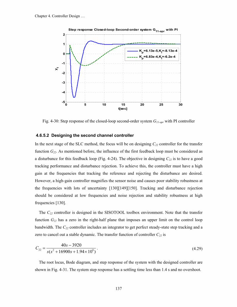
Chapter 4. Controller Design …
137
0 5 10 15 20 25 30-5
-4
-3
-2
-1
0
1
2Step response Closed-loop Second-order system G11-apr with PI
t[sec]
y 1
Kp=6.13e-5,KI=-8.13e-4
Kp=6.83e-4,KI=-6.2e-4
Fig. 4-30: Step response of the closed-loop second-order system G11-apr with PI controller
4.6.5.2 Designing the second channel controller
In the next stage of the SLC method, the focus will be on designing C22 controller for the transfer
function G22. As mentioned before, the influence of the first feedback loop must be considered as
a disturbance for this feedback loop (Fig. 4-24). The objective in designing C22 is to have a good
tracking performance and disturbance rejection. To achieve this, the controller must have a high
gain at the frequencies that tracking the reference and rejecting the disturbance are desired.
However, a high-gain controller magnifies the sensor noise and causes poor stability robustness at
the frequencies with lots of uncertainty [130][149][150]. Tracking and disturbance rejection
should be considered at low frequencies and noise rejection and stability robustness at high
frequencies [130].
The C22 controller is designed in the SISOTOOL toolbox environment. Note that the transfer
function G22 has a zero in the right-half plane that imposes an upper limit on the control loop
bandwidth. The C22 controller includes an integrator to get perfect steady-state step tracking and a
zero to cancel out a stable dynamic. The transfer function of controller C22 is
The root locus, Bode diagram, and step response of the system with the designed controller are
shown in Fig. 4-31. The system step response has a settling time less than 1.4 s and no overshoot.
22 2 840 3920
( 16900 1.94 10 )sC
s s s−
=+ + ×
. (4.29)

Chapter 4. Controller Design …
138
100
102
104
106
-180
0
180
360
P.M.: 58.5 degFreq: 3.17e+004 rad/sec
Frequency (rad/sec)
-150
-100
-50
0
50
G.M.: 30 dBFreq: 1.1e+003 rad/secStable loop
Open-Loop Bode C22
-4 -2 0 2 4
x 104
-2
-1.5
-1
-0.5
0
0.5
1
1.5
2x 10
5 Root Locus C22
Real Axis
(a)
Step Response of closed-loop system G22 with C22
Time (sec)
Am
plitu
de
0 0.2 0.4 0.6 0.8 1 1.2 1.4 1.6 1.8-0.2
0
0.2
0.4
0.6
0.8
1
1.2
Ref.
(b)
Fig. 4-31: Closed-loop G22 system with controller C22 , (a) root locus and bode diagram, (b) step
response

Chapter 4. Controller Design …
139
Fig. 4-32 illustrates the Bode plot of the second loop gain, i.e., L22=G22×C22. The figure reveals
that the second closed-loop system has a high gain at low frequency for good tracking and
disturbance rejection and low gain at high frequency for stability robustness and sensor noise
rejection.
10-2
100
102
104
-40
-20
0
20
40
60
80Bode Plot (G22C22)
Frequency (rad/sec)
Mag
nitu
de (d
B)
Fig. 4-32: Bode plot of the loop gain of the system G22 and controller C22
In order to verify the MIMO closed-loop system performance with the controller designed by
SLC method, the Singular Value Decomposition (SVD) index, that was defined in the pervious
chapter, is employed to find the maximum and minimum of the system loop gain. The large/small
SVD means large/small gain of a system. The SVD of the MIMO closed-loop system loop gain is
illustrated in Fig. 4-33. The system has a large SVD at low frequencies and a small SVD at high
frequencies. Therefore, the MIMO closed-loop system has a good tracking and disturbance
rejection at low frequency and good sensor noise rejection and stability robustness at high
frequency.

Chapter 4. Controller Design …
140
10-3
10-2
10-1
100
101
102
-40
-20
0
20
40
60
80Singular Values of the MIMO Closed-Loop Sysem
Frequency (rad/sec)
Max
and
nin
sin
gula
r val
ues
(dB
) (dB
)Max SVD
Min SVD
Fig. 4-33: SVD of the MIMO closed-loop system loop gain with SLC controller
4.6.6 Closed-Loop Wind Turbine Nonlinear Model with the SLC Controller
The linear controller designed with SLC is used to control the wind turbine system under study.
The linear and nonlinear system models are used in the simulations to follow. Fig. 4-34 shows the
schematic diagram of implementation of the closed-loop system in the Simulink/Matlab
environment. The closed-loop system responses to the step changes in the active and reactive
power references are shown in Fig. 4-35. The figure reveals a small discrepancy between the
linear and nonlinear model responses. Before applying the step change at t=1sec, the system is in
steady-state at the operating point. The step change is applied to the output active and reactive
power references at t=1 and 40 sec, respectively. The corresponding input control signals are also
illustrated in Fig. 4-36. As seen in Fig. 4-35, the system outputs follow the references with zero
steady-state errors. The control signals in Fig. 4-36 show that the frequency control signal
strongly affects the active power, while the input power factor signal is almost constant during
real power changes. On the other hand, the output reactive power variation is more sensitive to
the variations of input power factor control signal.

Chapter 4. Controller Design …
141
Fig. 4-34: Block diagram of the closed-loop system in the Simulink/Matlab
0 10 20 30 40 50 60 70 8082
84
86
88
90Step change ∆ P=1[kW] at t=1[sec],∆ Q=1[kVar] at t=40 [sec]
y 1=P [k
W]
0 10 20 30 40 50 60 70 8094
95
96
97
98
t[sec]
y 2=Q [k
Var
]
Linear Sys.Nonlinear Sys.
Pref
Qref
Fig. 4-35: Comparison of the linear and nonlinear closed-loop system responses to step changes
in references

Chapter 4. Controller Design …
142
0 10 20 30 40 50 60 70 80375
380
385
390
The control signels u1 and u2 for step change in the output references
u 1 [rad
/sec
]
0 10 20 30 40 50 60 70 800.598
0.6
0.602
0.604
t[sec]
u 2
Fig. 4-36: The control signals variations when step changes are applied to the output references

Chapter 4. Controller Design …
143
4.7 Summary
A closed-loop feedback controller, based on the linear model, is designed. The open-loop system
is locally stable around the operating point, and the controller design objective is to track a class
of desired active and reactive powers delivered to the grid. Two control design methods are
adopted for the wind turbine system: a state-feedback controller and an output-feedback
controller.
In the state-feedback controller, since the goal is to achieve zero steady-state error for the
family of step reference signals, first an integrator is added after the system. The combination of
the system with the integrator forms the augmented plant. Then, the state-feedback controller is
designed based on the LQ method. The LQ method is proved to be simple and effective for
adjusting the parameters of the closed-loop controller. The LQ method involves choosing
weighting matrices that minimize a cost function and provide satisfactory closed-loop
performance. The closed-loop performance depends on the location of the system eigenvalues in
the s-plane, and the locations of the eigenvalues are dependent on the weighting matrices in the
LQ method. For a high-order system, the number of Q and R elements is large, and finding the
best weighting matrices by trial and error to achieve a desired transient performance is difficult.
A genetic algorithm (GA) is used to determine the weighting matrices of the LQ method to
locate the closed-loop eigenvalues as close to the desired values as possible. The simulation
results reveal that the system with the closed-loop controller, designed by LQ and GA methods,
can satisfy the design constraints.
The state-feedback controller needs to measure all state variables. However, it is impractical to
measure all state variables in the system under study. Therefore, an observer is designed and used
in the state-feedback loop. The observer estimates the states by measuring the output and input
variables. The inputs of the observer block are the system input and output vectors, and its output
is the estimated state variables. The simulation results show that the observer affects the system
transients, but it has no effect on the steady-state (tracking) response. However, the gain and
phase margins are dramatically decreased when the observer is added to the system. In fact, the
observer increases the bandwidth of the controller. Because the system has some zeros in the
right-half plane, the high-bandwidth controller causes a big undershoot and decreases the phase-
margin.
Two other controllers based on the transfer function techniques are developed for the wind
turbine system.

Chapter 4. Controller Design …
144
First, a simple approach, based on decoupling the system at DC, is adopted. The controller is
carefully designed for the system, but the final controller results in an unstable closed-loop
system. This instability occurs consequent to the cross-channel interactions. To decrease the
effect of cross-channel interactions, the controller bandwidth in each channel should be
decreased. The closed-loop system becomes stable by trial and error and reducing the gain of the
controller. However, reducing the controller gain increases the system settling time.
Second, a sequential loop closure method is used to design a MIMO controller without ignoring
the cross-channel interactions at a certain frequency. By ignoring a weak cross-channel coupling,
the transfer function of the system under study can be converted to a triangular form. The SLC
controller design begins with designing an SISO controller for the channel that has no cross-
channel interactions with other channels. Then, the design will continue to the next channel while
taking into account the effect of the previously-designed channel as a disturbance. For simplicity
in controller design, the first channel transfer function is approximated by a second-order system.
A PI controller is designed for the second-order system to satisfy the design conditions. The
second loop controller is designed so that the closed-loop system has a high gain at low
frequencies which yields good tracking and disturbance rejection. Also, the closed-loop with
second loop controllers has low gain at high frequencies which yields stability robustness and
sensor noise rejection. The SVD index reveals that the final MIMO closed-loop system with the
SLC controller has a good tracking and disturbance rejection as well as a reasonable sensor noise
rejection and stability robustness.
Finally, the controller based on the SLC method is used in the closed-loop nonlinear MIMO
system. The simulation results are compared with those of the wind turbine linear model. The
results indicate that the system outputs follow the references with zero steady-state errors, and
there is a small discrepancy between the linear and nonlinear model responses. In addition, the
control signals show that the frequency control signal strongly affects the active power, while the
input power factor control signal is almost constant during real power changes. On the other hand,
the output reactive power variation is more sensitive to the variations of input power factor
control signal.

145
Chapter 5 Maximum Power Point Tracking Control for the Proposed Wind Turbine System
5.1 Introduction
This chapter focuses on the maximum wind power extraction algorithm, or Maximum Power
Point Tracking (MPPT) control, for the proposed wind energy conversion system. At a given
wind velocity, the mechanical power available from a wind turbine is a function of its shaft speed.
To maximize the power captured from the wind, the shaft speed has to be controlled. In order to
track maximum power, the matrix converter (MC) adjusts the induction generator terminal
frequency, and thus, the turbine shaft speed. The MC also adjusts the reactive power transfer at
the grid interface towards voltage regulation or power factor correction. A MPPT algorithm is
integrated in the closed-loop control system designed in the previous chapter, to control the MC
in order to capture maximum wind power.
In the next section, the concept of the MPPT in the wind energy conversion systems is
presented. Three existing maximum wind power extraction methods, Perturbation and
Observation (P&O), Wind Speed Measuring (WSM), and Power Signal Feedback (PSF), are
reviewed in Section 5.3. In Section 5.4, the implementation of P&O method for the proposed

Chapter 5. Maximum Power Point Tracking …
146
wind turbine system is introduced. Section 5.5, presents power signal feedback method, called
sensor-less PSF, for the wind turbine system under study. The claims made for the capabilities of
the proposed scheme are supported by analysis and simulation results.
5.2 Maximum Power Tracking Concept
In this section, the concept of Maximum Power Point Tracking (MPPT) is presented. The
variable-speed wind turbine (VSWT) was introduced in Chapter 1. At a given wind velocity, the
mechanical power available from a wind turbine is a function of its shaft speed. To maximize the
power captured from the wind, the shaft speed has to be controlled by a variable-speed method.
As mentioned in Chapter 1, the variable-speed wind turbine (VSWT) provides more energy
output, lower mechanical stress, and less power fluctuations, compared to the constant-speed
turbine.
The equations of the wind turbine mechanical power and mechanical torque were given in
Chapter 3 (see equations (3.1) and (3.2)). The wind turbine mechanical output power, PT is
affected by the ratio of the turbine shaft speed and the wind velocity, i.e., tip-speed-ratio
(λ=RωT/VW). As a result of variations in wind velocity, the turbine shaft speed ωT (or generator
shaft speed ωg), and wind turbine power PT will change. Fig. 5-1 shows a family of typical PT
versus ωr curves for different wind velocities for a typical system. As seen in this figure, different
power curves have different maximum power, Pmax (or optimal power, Popt).
Wind Turbine Power-versus-Turbine speed
Win
d Tu
rbin
e Po
wer
PT(k
Wat
)
Turbine Shaft Speed, ωT (rad/sec)
VW1
VW2
VW3
POpt VW3>VW2>VW3
Fig. 5-1: Wind turbine mechanical output power versus shaft speed

Chapter 5. Maximum Power Point Tracking …
147
In Fig. 5-1, the shaft speed maxPω corresponding to the maximum power is obtained from the
following equation:
0max
=∂∂
P
TPω
(5.1)
Substituting equation (3.1) and (3.4) from Chapter 3 in (5.1), yields:
12 2
15 0.3 0.00184 (15 0.3 )( cos ( ) 3)0.5 (0.44 0.0167max
wP
W
VR V
β β βωπ π ρ β
−− −⎛ ⎞= +⎜ ⎟ −⎝ ⎠ (5.2)
From (3.1) and (5.2) the maximum mechanical output power formula is:
( )maxmax T PP P ω= (5.3)
From mechanical design point of view, wind turbines are designed to operate at maximum
power for an average wind speed. However, it is clear that wind speed dose not stay at an average
level all the time. At lower wind speeds, tip speed ratio (λ) is increased (with constant rotor
speed), and accordingly, the power coefficient Cp decreases (equation (3.4)). As a consequence,
the wind turbine is not operating under optimal conditions (where Cp is low) most of the time.
Optimal operating conditions can be achieved by employing a MPPT method. Implementing a
MPPT method depends on wind turbine structure; however, these methods can be roughly
classified into three types [153]-[155]. In the following section, different MPPT methods are
discussed.
5.3 Maximum Power Point Tracking Methods
A literature survey identifies three common MPPT methods namely, perturbation and observation
(P&O) [106], wind speed measurement (WSM) [153], and power signal feedback (PSF)
[16][154]. In the following, these three methods are briefly explained.
5.3.1 Perturbation and Observation Method
The Perturbation and Observation (P&O) or Hill-Climb Searching (HCS) method is based on
perturbing the turbine shaft speed in small steps and observing the resulting changes in turbine
mechanical power [106][154].
The concept and schematic diagram of the P&O method is shown in Fig. 5-2. If the shaft speed
increment (∆ωT) results in a turbine power increment (∆PT), the operating region is in the up-hill

Chapter 5. Maximum Power Point Tracking …
148
curve, and increasing shaft speed must be continued toward maximum power point; otherwise,
the turbine operating region is in the down-hill curve, so the shaft speed should be decreased by
the P&O method to reach the maximum power point. To implement the P&O method, one can
check the signs of (∆ωT) and (∆PT/∆ωT). The shaft speed is incremented (∆ωT>0) in small steps
as long as (∆PT/∆ωT)>0 or decremented (∆ωT<0) in small steps as long as (∆PT/∆ωT)<0. This is
continued till maximum power point is reached, i.e., (∆PT/∆ωT)=0. If incrementing shaft speed
results in (∆PT/∆ωT)<0 or decrementing shaft speed results in (∆PT/∆ωT)>0, the direction of shaft
speed change must be reversed [106].
Tω
TP
TP∆Tω∆
xT MaPTP
Tω
Fig. 5-2: P&O method: (a) turbine power versus shaft speed and principle of the P&O method (b)
block diagram of the P&O control in wind turbine
The superiority of P&O method to other MPPT methods is in that it does not require priori
knowledge of the maximum wind turbine power at different wind velocities, and electrical
machine parameters [106][153][157]. However, P&O method is suitable for systems with small
inertia (small time-constant) [12][158], such as solar energy conversion systems with no inertia
or low-power and low-inertia wind turbine systems [156]. For medium and large-inertia wind
turbine systems, the turbine speed cannot follow changes in wind velocity; so, the P&O method
(without any other controller) will not be able to control the wind turbine system properly [154].
5.3.2 Wind Speed Measurement Method
The aim of the turbine speed control is to maintain turbine shaft speed at optimal value, i.e.,
maxPω , so that maximum mechanical power can be captured at any given wind velocity (VW)
[153][159]. In the wind speed measurement (WSM) method, both wind velocity and shaft speed
(ωT) should be measured. Also, optimal tip-speed-ratio (lopt) must be determined for the
controller. The block diagram of this method is shown in Fig. 5-3.

Chapter 5. Maximum Power Point Tracking …
149
Although this method is a simple method for implementing the MPPT, there are two drawbacks
to implementing the WSM method. First, obtaining accurate value of the wind velocity is
complicated and increases the cost of the system [153][160]. Second, the optimal tip-speed-ratio
is dependent on the wind energy system characteristics. Therefore, the controller will require
adjustment before installation in a new wind energy system [154].
WV
Wind TurbineSystemController
Tω
optλ maxPω
-
T
W
R
V
ωλ
×=
λ
+
Fig. 5-3: Block diagram of a wind energy system with shaft speed control using wind WSM
method
5.3.3 Power Signal Feedback (PSF) Control
The block diagram of a wind energy system with PSF control is shown in Fig. 5-4. In this
method, the maximum power curve of the wind turbine, Fig. 5-1, should be obtained first from
experimental results. Then, the data points for maximum output power and the corresponding
wind turbine speed must be recorded in a lookup table[154][160]-[162].
The concept of the PSF method is illustrated in Fig. 5-5. Tracking of the maximum power
curve, the dashed-curve, is the aim of the PSF method. Suppose the system is initially stable at
point A with wind velocity V1, shaft speed ωT1 and maximum output power P1. If the wind
velocity increases to V0, the new optimum power targeted by the controller should be P0. In the
moment following the wind velocity change, the shaft speed is still at ωT1, due to inertia of the
shaft. But, the turbine output power is increased to P'1, while the power reference based on the
lockup table is still P1. The shaft will accelerate under additional turbine torque and the operating
point is moved by the controller on the PT-ωT curve corresponding to V0 toward point B.
Eventually, the system will stabilize at point B with the new output power P0. Similar to this
scenario, if the system is settled down initially at point C and the wind velocity decrease to the V0,
the shaft decelerates toward ωT0.

Chapter 5. Maximum Power Point Tracking …
150
Wind EnergySystemController
Tω
_T OptP-
TP
Lookup Table
Tω
Fig. 5-4: Block diagram of a wind energy system with Power Signal Feedback control
Wind Turbine Power-versus-Turbine speed
Win
d Tu
rbin
e P
ower
PT (k
Wat
)
Turbine Shaft Speed, ωT (rad/sec)
V1
V0
V2
POpt
P1
P'1
P0P'
2
P2
ωT1 ωT0 ωT2
A
B
C
Fig. 5-5: The power signal control concept
To implement PSF control, the controller should be aware of the wind turbine maximum power
versus shaft speed curve. The maximum power is tracked by the shaft speed measurement and
corresponding power reference determination. No wind velocity measurement is required in this
method [154][162].
Although the PSF method does not require measuring the wind velocity, a barrier is the
difficulty of obtaining the maximum power curve of the wind turbine. Moreover, measuring the
mechanical shaft speed and wind turbine output power is another drawback of the PSF method.
In the following, a mechanical speed-sensorless PSF method is implemented in the wind
turbine system to overcome the mechanical shaft speed measurement requirement.

Chapter 5. Maximum Power Point Tracking …
151
5.3.4 Mechanical Speed-Sensorless PSF method
This subsection presents a maximum power tracking approach, called sensor-less PSF method.
The method has the capability of providing a power reference for the controller corresponding to
maximum power point without measuring the turbine shaft speed. In other words, the method is
based on PSF control, but neither wind velocity sensor nor turbine speed sensors are required.
This is the significant advantage of this method. The method can be developed for all wind-
turbine system including an induction-generator (I.G.) [16][163]-[165].
Fig. 5-6 shows the block diagram of a mechanical speed-sensorless PSF control system. In this
method a look-up table containing induction generator synchronous speeds (ωs) corresponding to
the optimal generator powers (Pgen-opt) is used. As the wind velocity keeps changing with time, the
wind turbine must keep adjusting its speed to track the optimum wind turbine speed. In the
following, the details of the sensorless PSF method are presented.
sω
. .I G
sω
Fig. 5-6 : Block diagram of the mechanical speed-sensoreless PSF control system
In the system under study the generator is connected to the turbine through a gearbox with gear
ratio ngear . Based on the turbine power-versus-turbine shaft speed (PT-versus-ωT) curves of Fig. 5-
1, the torque versus shaft speed at the generator side (Tg-versus-ωg) characteristics are shown in
Fig. 5-7. Note that in this figure, the quadratic optimal torque curve, Topt-vesus-ωg , is drawn
based on the following formula:
The dynamic behavior of the turbine and induction generator can be described as follows:
max
maxopt
P
PTω
= . (5.4)

Chapter 5. Maximum Power Point Tracking …
152
where TC(=-Tg) is the induction generator counter-torque and J is total shaft moment inertia
(including turbine and generator shaft inertia).
Wind Turbine Torque-versus-Turbine speed
Torq
ue a
t gen
rato
r sid
e (N
.m)
shaft speed at the genrator side, ωg (rad/sec)
ToptVW3
VW2
VW1
VW3>VW2>VW1
Tmax
Fig. 5-7: Wind turbine torque versus shaft speed on the generator side for different wind velocites
Maximum power production for any wind velocity is achieved when the generator counter-
torque equals optimal turbine torque (Topt). The equilibrium shaft speed can be found graphically
as the intersection of turbine torque-speed curve with generator torque-speed curves as illustrated
in Fig. 5-8 [106]. In this figure, the PT-versus-ωT and TT-versus-ωT curves of the wind turbine, as
well as a family of Tc-versus-ωg curves for the induction generator for different generator
synchronous speeds (ωs) are shown. Note that all curves are drawn on the same side of the
gearbox. By varying the output frequency of the converter (ωe), and thus, induction generator
synchronous speed (ωs), the Tc-versus-ωg curve can be shifted to the right or left with respect to
the wind turbine torque-speed curve to assume a wide range of possible steady-state operating
points defined by the intersections of the two curves. Obviously, one of the operating points
gT c
dT T J
dtω
− = . (5.5)

Chapter 5. Maximum Power Point Tracking …
153
corresponds to maximum power. To move from one operating point to another, ωe is changed in
steps (small enough to maintain generating mode) and the difference between the wind turbine
torque TT and the new generator counter torque Tc at the operating speed will accelerate or
decelerate the shaft according to equation (5.5) until the new steady-state operating point is
reached. In the following, moving towards maximum power point starting on two different sides
of optimal operating point are presented [106].
0 .33 .66 1 1.33 1.66-1.5
-1
-.5
0
.5
1
1.5
2
2.5
Shaft Speed ωr [p.u.]
TT Tc
Torq
ue [p
.u.]
PT
Pow
er [p
.u.]
P T
T T
OP1
OPopt
OP2
1
ωs1
ωsopt
ωs2
Optimal TC Tc=-Tg
ωr/ωr-opt
Fig. 5-8: Maximizing captured wind power by shifting Tc - ωr curve with respect to TT - ωr curve
A. Accelerating Shaft towards Maximum Power Point
In Fig. 5-8, OPopt is the operating point corresponding to maximum power captured from the wind
at the wind velocity of VW. At this point PT =1 [p.u.], TT =1 [p.u.], and ωr = optrω =1[p.u.], where
optrω is the angular shaft speed corresponding to maximum power point.
Assuming the present operating point to be OP1, corresponding to ωs1, the shaft should speed
up so that the operating point OPopt can be assumed by the system. This can be achieved by

Chapter 5. Maximum Power Point Tracking …
154
increasing ωs from ωs1 to optsω through an increase in the induction generator terminal frequency.
The frequency adjustment is performed in steps small enough for the induction machine to keep
operating as a generator throughout the transition period. This action makes TT-Tc>0 and
accelerates the shaft according to equation (5.5) towards maximum power point.
B. Decelerating Shaft towards Maximum Power Point
Assuming the present operating point to be OP2, corresponding to ωs2, the shaft should slow
down so that the system assumes the operating point OPopt. This can be accomplished by
decreasing ωs from ωs2 to optsω through a decrease in the induction generator terminal frequency
and voltage according to constant V/f strategy, in steps small enough to restrict operation within
the stable generating region. This action makes TT-Tc<0 and decelerates the shaft according to
equation (5.5) towards maximum power point.
5.3.4.1 The Maximum Power Point Data in the Mechanical Sensorless PSF Method
In the following, a formula for the optimal Popt-versus-ωs curve will be derived and the
corresponding data of the curve will be entered in the lookup table of Fig. 5-6 [16][165].
The generator torque is a function of its terminal voltage, and ωs, and ωg, as given by equation
(5.6).
As mentioned in Chapter 3, section 3.5, the induction generator voltage terminal is adjusted by
the MC according to a constant V/f strategy. To satisfy this strategy, the magnitude of induction
generator terminal voltage should be varied linearly with synchronous frequency as follows:
where KW is a proportionality constant. This constant can be calculated based on the constant V/f
ratio, that was defined in equation (3.51), as follows:
where VGrid-rated is the grid rated voltage.
( , , )G s s gT f V ω ω= . (5.6)
( )s s W sV Kω ω= , (5.7)
W VF Grid ratedK k V −= , (5.8)

Chapter 5. Maximum Power Point Tracking …
155
Substituting (5.7) in equation (5.6), and using the induction machine equivalent circuit in
Chapter 3, Fig. 3-7, and equation (3.11), the generator torque can be written as a function of ωs
and ωg :
Note that, in the generating mode of the induction machine, ωs < ωg and sign of Tg is negative,
representing a counter torque.
At the shaft speed ωr, the optimal torque corresponding to the maximum acquisition power can
be found from the Topt-versus-ωr curve, Fig. 5-1. The system is at the maximum power point if the
induction generator counter-torque is equal to Topt :
Tg can be calculated using the induction machine equivalent circuit, Fig. 3-7, as follows:
where Ir is the rotor current and can be obtained from the equivalent circuit as
where Zs=rs+jωsLs is the stator impedance, Zr=rr(ωs/( ωs- ωr))+j ωsLr is the rotor impedance, and
Zm=jωsLM is the magnetizing impedance.
Using equation(5.10), for a given optimal turbine torque and mechanical shaft speed
(optg gω ω= ), the corresponding generator synchronous speed (
opts sω ω= ) can be determined. In
other words, by solving equation (5.10) it is possible to plot the Topt–versus-optsω curve.
Employing this curve, instead of Topt–versus-optgω , makes the system speed-sensorless, because
there is no need to measure the mechanical speed ωg.
The lookup table in Fig. 5-6, contains the data points of Pgen_opt-versus-optsω curve, that can be
obtained easily from the Topt-versus-optsω curve as follows.
The optimal turbine power is:
( , )g g rT f ω ω= . (5.9)
( )opt g gT Tω = − . (5.10)
23 r rg
s g
r IT
ω ω=
−, (5.11)
( )( )
s s mr
s R m m r
V ZI
Z Z Z Z Zω
=+ +
, (5.12)

Chapter 5. Maximum Power Point Tracking …
156
Pgen_opt can be calculated using the induction machine equivalent circuit as
where Pmech_loss represents mechanical losses, Is and Ir are induction generator stator and rotor
currents, and 23 s sr I and 23 r rr I are copper losses in the stator and the rotor, respectively. Note that
the stator current can be determined as
Finally, the amounts of Pgen_opt -versus-optsω should be entered in the lookup table of Fig. 5-6.
The flowchart of Fig. 5-9 shows briefly the stages of finding the lookup table for implementing
using the mechanical speed-sensorless PSF method.
( , , )( , )
( )g s s g
g s gs s W s
T f VT f
V Kω ω
ω ωω ω= ⎫
=⎬= ⎭ @ 0 ( )W
TV cte opt g
g
T T fδ ωδω = = ⇒ =
( )optopt g opt sT T T f ω= − ⇒ =
2 2_ _( ) ( ) 3 3
opt opt
opt
gen opt s opt g mech loss s s r r
s
Evaluating P P P r I r I
at different values
ω ω
ω
= − − −
_ optgen opt sPuting thedata P and
in lookup table
ω
Fig. 5-9: Stages of finding the lookup table in the mechanical sensorless PSF method
( ) ( )opt opt optopt g opt g gP Tω ω ω= . (5.13)
2 2_ _( ) ( ) 3 3
opt optgen opt s opt g mech loss s s r rP P P r I r Iω ω= − − − , (5.14)
s ms r
m
Z ZI IZ+
= . (5.15)

Chapter 5. Maximum Power Point Tracking …
157
5.4 Implementing the P&O Method for a Small Wind Turbine System including a Matrix Converter
As mentioned in the pervious section, P&O method is suitable for the wind turbines with small
inertia. Therefore, other MPPT methods should be employed in the wind turbine under study. In
this section, in order to evaluate the P&O method, a wind turbine system including an induction
generator and an MC, with small inertia, is considered. Selected simulation results obtained from
the low-power wind turbine system under study are presented in this section; the detailed
explanations are given in [106]. Note that in [106], instead of a conventional MC, an improved
MC topology which does not have any commutation problems was adopted for the small wind
turbine system. The MC state-space dynamic model that was developed in Chapter 2 is a valid
model for the improved MC.
The structure of the system is the same as in Fig. 5-6, except for the controller which is based
on P&O method. The system parameters are shown in Appendix L. To assess the capability of the
P&O method in tracking the maximum power point at varying wind velocity, a step change is
applied to the wind velocity. The system is first operating at the wind velocity of Vw1=8m/s. At
this velocity, the optimal power captured from the wind turbine is 37kW. At t=1.8s, the wind
velocity is decreased to 6m/s. The optimal power corresponding to this velocity is 15kW. Again,
at t=2.5s, the wind velocity is increased back to 8m/s. Fig. 5-10 illustrates successful tracking of
maximum power using the P&O method following the changes made to the wind velocity. Fig. 5-
11 shows the variations in the matrix converter output frequency set-point that results in the
necessary changes in the induction generator terminal frequency and thus the shaft speed in
attempt to track the maximum power point. It has to be noted that the magnitude of the induction
generator terminal voltage has been varied with frequency according to the constant V/f strategy.
Also, the displacement power factor at the interface with the grid has been maintained at unity at
steady-state, using matrix converter control.
As mentioned, this method does not require priori knowledge of maximum wind turbine power
at different wind velocities, and induction machine parameters. Also, using this method,
maximum power point can be reached irrespective of the present operating point, while
maintaining the operation in the stable generating region during transitions.

Chapter 5. Maximum Power Point Tracking …
158
0.5 1 1.5 2 2.50.5
1
1.5
2
2.5
3
3.5
4x 10⁴
PG
rid(k
Wat
)
Time[sec]
Popt=37(kWat) P
opt=37(kWat)
Popt=15(kWat)
PGridPopt
Fig. 5-10: Maximum power point tracking control at varying wind velocity with P&O method
0.5 1 1.5 2 2.5 330
35
40
45
50
55
60
Set
-poi
nt fr
eque
ncy
of M
c [H
z]
Time[sec]
Fig. 5-11: Frequency set point variations during maximum power point tracking with P&O
method

Chapter 5. Maximum Power Point Tracking …
159
5.5 Implementing the Mechanical Speed-Sensorless PSF Method on the Wind Turbine System under Study
In this section, simulation results of the wind turbine system under study including the
mechanical speed-sensorless power signal feedback are presented. The parameters of the wind
turbine system are given in Appendix L.
To implement the mechanical speed-sensorless PSF method, based on block diagram Fig. 5-6,
first, the curves Topt(ωg) (Fig. 5-7) and Topt(ωs , ωg) (equations (5.6) and (5.7)) should be
determined. Second, the lookup table data can be obtained based on flowchart of Fig. 5-9.
In the wind turbine system, it is easier to measure the grid power instead of the power at the
generator output terminals. Therefore, for implementing the speed-senseless PSF method on the
system, the grid optimal power, PGrid_opt , should be entered in the lookup table. The PGrid_opt(ωs)
curve can be calculated by subtracting MC active power losses from the Pgen_opt at each
synchronous frequency. Fig. 5-12 shows the curves PT_opt-versus-ωs and PGrid_opt-versus-ωs for the
system under study.
250 300 350 400 450 500 550 6000
50
100
150
200
250
P[Kw
at]
ωs-ref [rad/Sec] synchronous frequency at the genrator side
PT-opt
PGrid-opt
Total power losses
Fig. 5-12: PTopt(ωs) and PGrid_opt(ωs) curves

Chapter 5. Maximum Power Point Tracking …
160
The schematic diagram of the wind turbine system with the speed sensor-less PSF, in
Matlab/Simulink environment, is shown in Fig. 5-13.
Fig. 5-13: Block diagram of the wind turbine system with the mechanical speed-sensorless PSF
in Matlab/Simulink
The system is originally stable at an operating point with wind velocity of 10 m/s before
applying the maximum power point tracking (MPPT) method. Table 5.1 shows the input and
output parameters of the system at the operating point.
Table 5.1: Parameters of the wind turbine system at the operating point
Voltage
Gain
Output voltage
angle
MC output
frequency
Rotor pitch
angle Wind speed Grid powers
q=0.5 αο=0 fo_MC = 6o Hz β=0 VW=10[m/s] PGrid= 80.82[kWat]
QGrid=56.42[kVar]
In the following simulations, the mean wind velocity will be changed to verify the capability of
the MPPT method used. Table 5.2 shows the maximum mechanical wind power and the grid

Chapter 5. Maximum Power Point Tracking …
161
active power reference for three different wind velocities. The controller should follow the
maximum power at each wind velocity.
Table 5.2: Maximum Power at different wind velocity
Wind velocity
[m/s]
WT Maximum Power
[kWat]
Grid Maximum Power
[kWat]
VW =10 PTopt= 86.39 PGrid,opt= 84.96
VW =11 PTopt= 114.99 PGrid,opt= 113.11
VW =12 PTopt= 149.29 PGrid,opt= 146.81
Note that in Table 5.2, the discrepancy between the wind turbine and the grid maximum power
is because of the system total losses.
Fig. 5-14 depicts the grid active power of the wind turbine system with the speed-sensorless
PSF at three wind velocities. The system works at the operating point, Table 5.1, initially. The
MMPT algorithm has stabilized the system at maximum power point corresponding to wind
velocity equals 10 m/s. Mean wind velocity is then increased to 12 m/s at t=30s, decreased to
11m/s at t=60s, and finally decreased to 10 m/s at t=90s. The wind turbine system tracks the
maximum power corresponding to different wind velocities successfully. At the same time, the
grid reactive power and synchronous speed of induction generator are controlled by the MC. The
reactive power of the grid is kept almost constant by the MC as shown in Fig. 5-15. Fig. 5-16 and
Fig. 5-17 illustrate the electrical synchronous speed of the generator, which is adjusted by the
MC, and the mechanical shaft speed of the turbine, respectively, in response to the wind velocity
variations.
Also, as shown in Fig. 5-14, the settling time of the system with the MPPT method, for the step
change, is about 8s. In other words, the system can track the maximum power point for the mean
wind speed changes that take place at frequencies lower than approximately 1/8 Hz.

Chapter 5. Maximum Power Point Tracking …
162
0 10 20 30 40 50 60 70 80 90 100 11080
90
100
110
120
130
140
150Grid active power
P Grid
[kW
at]
time[sec]
PGridopt
PGrid
Fig. 5-14: Grid active power for the wind turbine system including speed-sensorless PSF method
0 10 20 30 40 50 60 70 80 90 100 11040
45
50
55
60
65Grid Rective Power
QG
rid [k
Var
]
time[sec]
Fig. 5-15: Grid reactive power for the wind turbine system including speed-sensorless PSF
method
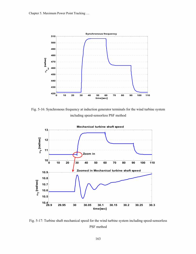
Chapter 5. Maximum Power Point Tracking …
163
0 10 20 30 40 50 60 70 80 90 100 110420
430
440
450
460
470
480
490
500
510Synchronous frequency
ωs op
t [rad
/sec
]
time[sec]
Fig. 5-16: Synchronous frequency at induction generator terminals for the wind turbine system
including speed-sensorless PSF method
0 10 20 30 40 50 60 70 80 90 100 11010
11
12
13
ωT [r
ad/s
ec]
Mechanical turbine shaft speed
29.9 29.95 30 30.05 30.1 30.15 30.2 30.25 30.310.4
10.5
10.6
10.7
10.8
10.9
ωT [r
ad/s
ec]
time[sec]
Zoomed in Mechanical turbine shaft speed
Zoom in
Fig. 5-17: Turbine shaft mechanical speed for the wind turbine system including speed-sensorless
PSF method

Chapter 5. Maximum Power Point Tracking …
164
Fig. 5-18 shows the range of variation of wind speed over which maximum power point can be
successfully tracked. Accordingly, the minimum wind speed at which the wind turbine injects
active power into the grid, is 3m/s corresponding to maximum grid power of 1.04kW. The
maximum wind speed limit of the system is 22m/s corresponding to a maximum grid power of
838.82kW. Therefore, the system with the adopted MPPT method is capable of tracking the
maximum power in response to a step decrease to VW=3m/s and a step increase VW=22m/s from
the operating point (VW=10m/s, PGrid,opt=84.96kW). At wind velocities below 3m/s, the direction
of the active power flow will be from the grid to the wind turbine because the electrical machine
operates in motoring mode. If the wind speed exceeds 22m/s, the controller will not be able to
track maximum power.
0 10 20 30 40 50 60 70 80 90 1000
100
200
300
400
500
600
700
800
900Generator active power
Gri
d ac
tive
Pow
er [k
W]
time[sec]
VW=3m/sPGrid
opt=1.04kW
VW=10m/sPGrid
opt=84.96kW
VW=22m/sPGrid
opt=838.82kW
Fig. 5-18: Maximum and minimum levels of grid active power for the wind turbine system
including speed-sensorless PSF method
The simulation results show that the controller including the mechanical sensorless PSF
method has a high capability to track the maximum power point at different wind velocities.
However, accuracy of the method depends on the data obtained for the lookup table.

Chapter 5. Maximum Power Point Tracking …
165
5.5.1 Evaluation of the Mechanical Speed-sensorless PSF method with the instantaneous wind velocity
In Subsection 3.2.6, the wind velocity model was described as the wind speed average value plus
a stochastic fluctuation of the wind velocity, equation (3.23). Also, the high-frequency damping
phenomenon was considered in the final wind velocity model to be used in the wind turbine
model, as shown in Fig. 3-12.
In the previous simulations of Section 5.5, the wind velocity was considered to be a constant
signal with some step changes. In this subsection, the controller including the speed-sensorless
PSF method is evaluated with an instantaneous wind velocity model. The wind velocity signal
(VW) and the grid active response (PGrid), as well as the optimal synchronous speed, are depicted
in Fig. 5-19. As shown in this figure, the mean value of the instantaneous wind velocity is
increased from 10m/s to 11m/s at t=20s. In each instance, the system follows the instantaneous
wind velocity variations and the controller leads the system toward the maximum power point
based on the mean wind velocity. The simulation results reveal that the controller including the
speed-sensorless PSF method is capable of working with the instantaneous wind velocity.
0 5 10 15 20 25 30 35 408
10
12Wind Speed
Spee
d [m
/s]
5 10 15 20 25 30 35 4080
100
120Grid active power
PG
rid[k
Wat
]
5 10 15 20 25 30 35 40400
450
500Synchronous frequency
ωs op
t [rad
/sec
]
time[sec]
mean VW VW
Fig. 5-19: Evaluating the system including the speed-sensorless PSF method with the
instantaneous wind model

Chapter 5. Maximum Power Point Tracking …
166
5.6 Summary
This chapter presented a maximum power point tracking (MPPT) method for the proposed wind
turbine system. The controller including the MPPT method controls the shaft speed to maximize
the power captured from the wind. This is possible by adjusting the MC output frequency. The
output voltage is adjusted according to constant V/f strategy. The controller also adjusts the MC
variables to control the reactive power transfer at the grid interface to regulate the power factor.
The concepts of three MPPT methods, Perturbation and Observation (P&O), Wind Speed
Measuring (WSM), and Power Signal Feedback (PSF) are reviewed.
The P&O method is a continuous search algorithm to track the maximum power point. The
P&O method does not require prior knowledge of the maximum wind turbine power at different
wind velocities, or electrical machine parameters. However, this method is suitable for wind
turbine systems with very small inertia that can respond quickly to shaft speed change requests.
The wind speed measurement (WSM) method regulates the shaft speed to keep the turbine at
an optimal tip-speed-ratio (lopt). In this method, both wind velocity and shaft speed (ωT) should
be measured. Also, lopt must be given to the controller. This method suffers two drawbacks:
difficulty of measuring the wind velocity and dependence of lopt on the wind turbine
characteristics.
In the PSF method, the controller should be aware of the wind turbine maximum power versus
shaft speed curve. In this method, the maximum power is tracked by the shaft speed measurement
only and no wind velocity measurement is required. However, the difficulty of obtaining the
maximum power curve of the wind turbine, and measuring the mechanical shaft speed and wind
turbine output power are the drawbacks of the PSF method.
A developed power signal feedback method, called speed-sensorless PSF, is proposed for the
wind turbine system under study to improve the PSF method. The method needs neither a wind
velocity sensor nor a turbine speed sensor. Simulation results show successful tracking of
maximum power at all wind velocities.

167
Chapter 6 Conclusions
6.1 Summary and conclusions
In this thesis, a wind energy conversion system including a matrix converter (MC) is proposed. A
squirrel-cage induction generator (SCIG) is selected because of its low-cost, robustness and high
reliability for wind turbines. The wind turbine is followed by a gearbox which steps up the shaft
speed. MC interfaces the SCIG with the grid and transfers the entire power generated by the wind
turbine to the grid. Also, MC controls the terminal voltage and frequency of the induction
generator, based on a constant V/f strategy, to adjust the turbine shaft speed, and accordingly,
control the active power injected into the grid to track maximum power at all wind velocities. The
power factor at the interface with the grid is also controlled by MC to either ensure purely active
power injection into the grid for optimal utilization of the installed wind turbine capacity or assist
in regulation of voltage at the point of connection. Furthermore, the reactive power requirements
of the induction generator are satisfied by MC to avoid use of self-excitation capacitors.
A dynamic model that represents the proposed system and a closed-loop controller to track the
desired active and reactive powers delivered to the grid are developed. The desired power is used
as the reference for the closed-loop control of the power injected into the grid. The controller uses
an algorithm to derive the maximum power that can be achieved at a given wind velocity. In
order to track maximum power, MC adjusts the induction generator terminal frequency, and thus
the turbine shaft speed. MC adjusts the reactive power transfer at the grid interface to achieve
voltage regulation or power factor correction.
Chapter 2 introduces MC and its overall dynamic model. An MC is highly controllable and
allows independent control of the output voltage magnitude, frequency, and phase angle, as well
as the input power factor. Compared with the DC-link AC/AC converter systems, an advantage of

Chapter 6. Conclusions
168
the MC is elimination of the DC-link, including bulky capacitors. Furthermore, the MC structure
is inherently capable of a four-quadrant operation. The developed dynamic model consists of six
nonlinear equations in the same frequency frame. The final state-space qdo dynamic model
contains six state variables and four control variables. Input and output active and reactive power
formulas are developed based on the model state variables. To evaluate the MC state-space qdo
dynamic model, first the model is simulated with Matlab/Simulink; then, the results are compared
with the simulation results of a model based on the MC fundamental-frequency equivalent circuit,
obtained from the PSIM simulation package. The results of the two models are fairly close. The
presented state-space model is comprehensive in the sense that it includes output voltage
magnitude, frequency and phase angle, as well as input displacement power factor, as control
variables. The proposed model can be used effectively in modeling electrical systems including
MC, for transient study, stability analysis, and systematic controller design.
Chapter 3 focuses on developing a comprehensive dynamic mathematical model of the
proposed wind turbine system to be used for controller design purposes. Detailed mathematical
models of the mechanical aerodynamic conversion, drive train, and squirrel-cage induction
generator are developed and combined with the MC model to enable steady-state and transient
simulations of the overall system. To avoid saturation of the induction machine when the stator
frequency is changed, the dynamic model is modified based on the constant V/f strategy. Steady-
state response of the model shows that the grid active and reactive power vary with the MC
output frequency. But, by varying the parameter that controls the displacement power factor, only
the grid reactive power is affected. Dynamic behavior of the model is investigated by simulating
the step responses to selected input variables.
Moreover, a linearized model of the wind turbine system is developed around an operating
point. The results show the local stability of the open loop system against the input variations
around the operating point. However, the step response of the system shows a type of
nonminimum-phase behaviour. The controllability and observability are evaluated at the
operating point and a reduced-order model that has performance close to the original model is
developed. It is concluded that the linear model is an appropriate model for the design of a
controller to improve the steady-state and transient performances of the system.
Chapter 4 is dedicated to the design of a closed-loop feedback controller based on the linear
model to track the desired active and reactive powers delivered to the grid. Two control design
methods are adopted for the wind turbine system: a state-feedback and an output-feedback
controller. In the state-feedback closed-loop system, first an integrator is added after the system

Chapter 6. Conclusions
169
model to achieve zero steady-state error for the step response. Then, the state-feedback controller
is designed based on the LQ method. The LQ method is effective for adjusting the parameters of
the closed-loop controller. A genetic algorithm (GA) is used to determine the weighting matrices
of the LQ method to locate the closed-loop eigenvalues as close to the desired values as possible.
The simulation results reveal that the system with the closed-loop controller, designed by LQ and
GA method, can satisfy the design constraints. Moreover, an observer is designed and used in the
state-feedback loop. The simulation results show that the observer affects the system transients,
but it has no effect on the steady-state (tracking) response. However, the gain and phase margins
are dramatically decreased when the observer is added to the system.
Two other approaches to design of the controller based on transfer function techniques are
adopted: DC decoupling and a sequential loop closure (SLC). The controller designed with DC
decoupling approach yields a low-gain controller that causes a long settling time that is not
acceptable. The simulation results with the SLC controller show good tracking and disturbance
rejection, as well as reasonable sensor noise rejection and stability robustness, for both linear and
nonlinear versions of the proposed model. In addition, the simulation results with SLC closed-
loop controller show that the frequency control signal strongly affects the active power, while the
input power factor control signal is almost constant during real power changes.
Chapter 5 presents the maximum power point tracking (MPPT) based on two methods:
Perturbation and Observation (P&O), and Power Signal Feedback (PSF). The P&O method is a
continuous search algorithm to track the maximum power point. The P&O method does not
require prior knowledge of the maximum wind turbine power at different wind velocities and
electrical machine parameters. However, this method is suitable for wind turbine systems with
very small inertia, that can respond quickly to shaft speed change requests. In the PSF method,
the controller should be aware of the wind turbine maximum power versus shaft speed curve. In
this method, the maximum power is tracked by shaft speed measurement only, and no wind
velocity measurement is required. However, the difficulty of obtaining the maximum power curve
of the wind turbine, as well as measuring the mechanical shaft speed and wind turbine output
power are the drawbacks of the PSF method. A developed power signal feedback method, called
speed-sensorless PSF, is proposed for the wind turbine system under study to improve the PSF
method. The method needs neither a wind velocity sensor nor a turbine speed sensor; but, it needs
the maximum power curve of the wind turbine. Simulation results show successful tracking of
maximum power at all wind velocities.

Chapter 6. Conclusions
170
6.2 Contributions
The focus of this thesis is on three main issues:
• Developing a dynamic model for MC and the proposed wind energy conversion
system,
• Designing a closed-loop controller for the proposed system, and
• Developing a maximum power point tracking method for the system under study.
This research is novel because it proposes the use of an MC in a wind turbine system and
develops a dynamic overall model and a maximum power point tracking controller for the
proposed wind turbine system.
The following outline the contributions of this thesis:
1. A wind energy conversion system based on an induction generator and a matrix converter,
that has not been thoroughly investigated before, is proposed.
2. A comprehensive state-space qdo dynamic model is developed for the MC. The main
contribution in this model is to include a control variable for input displacement power factor.
The model could be used effectively in modeling electrical systems including MC, for transient
study, stability analysis, and systematic controller design.
3. In the modeling of the proposed wind turbine system, the main contribution of this work is
developing an overall model that considers all electrical and mechanical control variables. The
model contains four control variables related to the MC and one for turbine blade pitch angle
control, and considers wind velocity as a disturbance input. Another contribution in this part is to
modify the dynamic model based on a constant V/f strategy to avoid saturation of the induction
machine when the induction generator stator frequency is changed.
4. In the linearized model, the main contribution is developing a reduced-order model of the
system based on the linearized model with a performance as close as possible to the original
model.
5. In the closed-loop state-feedback controller design, the main contribution of this work is
using the genetic algorithm (GA) in the linear-quadratic (LQ) method to satisfy the design
constraints perfectly.
6. For the proposed wind turbine, an output-feedback controller is designed based on an SLC
method. The main contribution of this part is adopting a simple method for designing the

Chapter 6. Conclusions
171
controller, first by ignoring a weak cross-channel coupling, and second by approximating a
channel by a second-order system and designing a PI controller. The designed controller has a
good transient and tracking performance, disturbance and sensor noise rejection, and stability
robustness.
7. In the maximum power point tracking controller design, the main contribution of this work is
to develop a method for the proposed system which needs neither a wind velocity sensor nor a
turbine shaft speed sensor. In this method, the electrical power injected to the grid is the only
measurement in the closed-loop system.
6.3 Suggestions for Future work
To continue and complete the work presented in this dissertation, one can focus on a number of
specific areas as follows:
• Experimental Test
A laboratory prototype of the proposed wind energy conversion system can be built and tested to
verify the validity of the developed dynamic model.
• Multilevel Matrix Converter
A multilevel MC is scalable to higher power and voltage levels. The purpose of using multilevel
MC is to improve the energy capture of the wind turbine. Studying the configuration and
switching strategy of multilevel MC, and developing a dynamic model of a wind turbine system
including a multilevel MC are suggested.
• Robust Control of the Wind Turbine System
To identify the wind turbine model parameters, the wind speed statistics should be collected at
each operating point during long intervals. The developed model is subject to parameter
uncertainty. In order to cope with the model uncertainties and design a controller accordingly, the
techniques of linear robust control theory should be used.
• Using Permanent Magnet (PM) Generator in the Proposed System
The progress in the permanent magnet materials fabrication has extended the PM generator
lifetime and decreased the production cost. This is a motivation for replacing the induction
generator (and gearbox) with a PM generator.

Chapter 6. Conclusions
172
• Intelligent Maximum Power Point Tracking (MPPT) Algorithm
An intelligent algorithm can be developed for MPPT with the following features:
- independent of the wind turbine characteristics, and thus flexible and effective, and
- trainable online to behave adaptively.

173
Appendix A Practical Bidirectional Switch Configuration for
the Matrix Converter For many years, thyristor have been the preferred semiconductor switch in power electronic
converters. To realize a bidirectional switch, two thyristors have to be connected in antiparallel.
In order to turn off the thyristor, force-commutating circuits should be used. This results in
increased size and complexity of circuits. As a result of development the new generation of
inherent gate-turn-off switches such as GTO, BJT, MOSFET and IGBT, as well as increasing
their power ratings, these switches have become a better choice than the thyristor. In order for an
MC to have capability of four-quadrant operation, bidirectional or four-quadrant switches are
required.
A four-quadrant switch is capable of blocking voltages of both polarities in OFF-state and
conducting currents in both directions in ON-state. Currently, there is no monolithic switch in the
market with this capability. In practice, the four-quadrant switch can be realized using power
diodes and gate-turn-off switches.
Fig A-1 illustrates three practical methods of realizing bidirectional switches with power diodes
and insulated bipolar junction gate transistor (IGBT). Table A-1 compares the three bidirectional
switch structures, i.e. diode bridge, common emitter and common collector. Among these three
possible bidirectional switch structures, the common-emitter configuration has minimized stray
inductance and is usually preferred in practice [97][98].

Appendix A. Practical Bidirectional Switch...
174
i +
-
ν
+
ν
-
i
ν
+
-
i
(a) (b) (c)
Fig. A-1: Three practical bidirectional switch configurations: (a) Diode bridge and one switch (b)
Common emitter and (c) common collector
Table A-1 comparison of bidirectional switch structures [97][98]
A MC circuit may be constructed from the bidirectional switch cell with discrete components.
It is also feasible to build a MC in a package with IGBT modules. The technology has moved in
the direction of developing a practical full MC power circuit in a single package. Some types of
single-package MC are now commercially available.
Structure Number of
components Advantages Disadvantages
Diode Bridge
and one switch 4 diodes 1 switch
One gate drive per switch cell
-High device losses -No control on the direction of
current by switch
Common
emitter 2 diodes 2 switches
Independent control of the direction of current
High number of isolated power supplies for the gate drives in MC models
Common
collector 2 diodes 2 switches
Reduce the number of isolated power supplies for the gate drives in MC module
High stray inductance

175
Appendix B Switch State Combinations in MC
Table B-1: 27 Switch state combinations in MC[55] Group Switches ‘ON’ VAB VBC VCA ia ib ic
I
SAa SBb SCc
SAa SBc SCb
SAb SBa SCc
SAb SBc SCa
SAc SBa SCb
SAc SBb SCa
vab vbc vca
-vca -vbc -vab
-vab - vca - vbc
vbc vca vab
vca vab vbc
-vbc -vab -vca
iA iB iC
iA iC iB
iB iA iC
iC iA iB
iB iC iA
iC iB iA
II-A
SAa SBc SCc
SAb SBc SCc
SAb SBa SCa
SAc SBa SCa
SAc SBb SCb
SAa SBb SCb
-vac 0 vca
vbc 0 -vbc
-vab 0 vab
vca 0 -vca
-vbc 0 vbc
-vab 0 -vab
iA 0 -iA
0 iA -iA
-iA iA 0
-iA 0 iA
0 -iA iA
iA -iA 0
II-B
SAc SBa SCc
SAc SBb SCc
SAa SBb SCa
SAa SBc SCa
SAb SBc SCb
SAb SBa SCb
vca -vca 0
-vbc -vbc 0
-vab - vab 0
-vca vca 0
vbc -vab 0
-vab vab 0
iB 0 -iB
0 iB -iB
-iB iB 0
-iB 0 iB
0 -iB iB
iB -iB 0
II-C
SAc SBc SCa
SAc SBc SCb
SAa SBa SCb
SAa SBa SCc
SAb SBb SCc
SAb SBb SCa
0 vca -vca
0 -vbc -vbc
0 -vab - vab
0 -vca vca
0 vbc -vab
0 -vab vab
ic 0 -iC
0 iC -iC
-iC iC 0
-iC 0 iC
0 -iC iC
iC -iC 0
III
SAa SBa SCa
SAb SBb SCb
SAc SBc SCc
0 0 0 0 0 0 0 0 0
0 0 0 0 0 0 0 0 0

Appendix B. Switch State Combinations
176
Based on Table B.1, the connections between input and output phases of MC can be classified in
three groups with different properties, as illustrated in Table B.2.
Table B.2: Classifications of switch state combinations of Table B.1
Number of combinations Special Feature
Group I 6 combinations Each output phase is connected to a different input phase
Group II 3×6 combinations Two output phases are shorted
Group III 3 combinations Three output phases are shorted

177
Appendix C Modulation Algorithm and SVPWM
There are two major modulation algorithms in the literature for controlling the switches in an MC,
i.e., direct and indirect methods [60].
C.1 Direct switching matrix approach
A transformation matrix D, whose elements are sinusoidal functions at frequency io ωω ± , makes a
direct connection between the input and output voltages and currents of MC. Thus, this method is
named direct method. In this method, one can prove that the maximum voltage gain is restricted to
0.5 instead of 0.87 [60]. Improving the feasible voltage ratio to 0.87 is possible by injecting the third
harmonics of the input and output frequencies into the desired output phase voltages as shown in
equation (C.1).
1 1cos(3 ) cos(3 )6 2 3cos( )1 1cos( 2 / 3) cos(3 ) cos(3 )6 2 3
cos( 2 / 3)1 1cos(3 ) cos(3 )6 2 3
o i
o
ABC om o o i
o
o i
t tt
v V t t tt
t t
ω ωω
ω π ω ωω π
ω ω
⎡ ⎤⎧ ⎫− +⎢ ⎥⎪ ⎪⎢ ⎥⎪ ⎪⎢ ⎥⎪ ⎪= − + − +⎨ ⎬⎢ ⎥
⎪ ⎪⎢ ⎥+ ⎪ ⎪⎢ ⎥− +⎪ ⎪⎢ ⎥⎩ ⎭⎣ ⎦
(C.1)
where ABCv is the MC output voltage vector, Vom is the peak value of MC output voltage, and ωi and
ωo are the input and output MC frequencies, respectively. These additional injected harmonics are
called common-mode voltages. Even though common-mode voltages cause nonsinusoidal output
phase voltages, they have no effect on the output line-to-line voltages and allow the desired voltage
gain to increase to 87% [60][65][99]. Adding the common-mode voltages makes analysis and
implementing the direct switching matrix method difficult. It is worth mentioning that this method
uses all combinations of the three groups in Table B.2.

Appendix C. Modulation Algorithm…
178
C.2 Indirect switching matrix approach
The indirect switching matrix approach or indirect modulation is based on a simplified modulator
model, making it feasible to implement classical PWM methods for MCs [55][97][99]. This method
is based on the fact that the MC, and its transfer switching matrix, are considered as an imaginary
two-stage transformation: rectification stage and inverter stage. In the rectification stage, a fictitious
dc link with a dc voltage of constant local average will be provided. Then, the fictitious dc voltage is
converted to the three-phase output voltages in inverter stage. One solution for the transformation
matrix D is as follows:
cos( ) cos( ). cos( 2 /3) cos( 2 /3) ( ). ( )
cos( 2 / 3) cos( 2 / 3)
To o i i
To o i i I o R i
o o i i
t tD m t t D D
t t
ω ϕ ω ϕω ϕ π ω ϕ π ω ωω ϕ π ω ϕ π
+ −⎡ ⎤ ⎡ ⎤⎢ ⎥ ⎢ ⎥= + − − − =⎢ ⎥ ⎢ ⎥⎢ ⎥ ⎢ ⎥+ + − +⎣ ⎦ ⎣ ⎦
(C.2)
In the above transformation matrix the )( oID ω is the 3×1 inverter transfer matrix which is a
function of output frequency, and the )( iRD ω is the 3×1 rectifier transfer matrix which is a function
of input frequency. The concept of the indirect method is illustrated in Fig. C-1 by six imaginary
switches for the rectifier part and six imaginary switches for the inverter part.
ai bi ci ABi BCi
CAi
anv bnv cnv
pnv
Fig. C-1: Two- stage MC with fictitious dc-link
To make the concept of fictitious dc voltage clear, one can multiply the input ac voltage vector
from (3-11) by )( iTRD ω . Then, a constant equivalent dc voltage is obtained as follow:

Appendix C. Modulation Algorithm…
179
[ ]
( )cos( )
cos( ) cos( 2 /3) cos( 2 / 3) cos( 2 /3)cos( 2 / 3)
1.5 cos( )
TR i iPh
i
i i i i i i im i
i
im i consta nt
D vt
t t t V tt
V
ωω
ω ϕ ω ϕ π ω ϕ π ω πω π
ϕ
=
⎡ ⎤⎢ ⎥+ + − + + −⎢ ⎥⎢ ⎥+⎣ ⎦
= × × =
(C.3)
Also three-phase output voltages will be produced by multiplying the constant voltage given in
(C.3) and inverter transfer matrix )( oID ω .
It follows from Fig. C-1 that the connection between the input and output phases is possible only
through the positive and negative rails of the fictitious dc link. Due to the operation of the inverter
stage, one of the following two switching conditions occurs at any given time:
• Two phases of the input and output connect to the same line ‘P’ or ‘N’, and
• Three phases of input or output connect to the same line ‘P’ or ‘N’.
These two possible conditions include all combinations of groups II and III, and none from the group
I, in Table B.2. Thus this method will realized only 21 switching combinations out of the 27
combinations in total. It is unlike direct matrix transfer approach that uses all combinations.
Reference [55] shows that the maximum voltage gain with indirect method is 3 / 2 , without
necessary harmonic injection into the transfer matrix.
The indirect method is well-known method for implementing PWM techniques in MC, like general
voltage source and current source converters, and it does not have the complexity of direct approach.
In the next section, a systematic PWM method based on indirect switching matrix approach is
reviewed.
C.3 Space Vector Pulse width Modulation Technique
The space vector-based pulse width modulation (SVPWM) technique is a well known method in
control of DC/AC converters [100]. The SVPWM offers a number of useful features, especially in
realistic implementation, such as:
• voltages or currents can be represented in two-dimension reference frames instated of
three-dimensional abc frames,
• reducing the number of switching in each cycle,
• better output waveforms compared with conventional PWM methods,

Appendix C. Modulation Algorithm…
180
• controllable PFin (input Power Factor) regardless of the PFout (load power factor),
• extending easily to multilevel inverters by inserting additional switching states, and
• SVPWM is a digital modulation technique and is easy to implement with digital
controller, while PWM is an inherently analogue technique.
SVPWM can be applied to MC in the same way that it is applied to DC/AC converter, but is more
complex in this case [55][60][62]. Based on the indirect matrix switching approach, the SVPWM can
be simultaneously applied to both output voltage at the inverter part and input current at the rectifier
part. In the following sections, the SVPWM procedures for both voltage- source inverter and current-
source rectifier are reviewed. Then, the steps for controlling the output voltages and inputs currents
are discussed.
C.5 SVPWM for controlling output voltages of voltage source inverter
Fig. C-2 illustrates the voltage source inverter (VSI) part of the MC circuit of Fig. C-1, with fictitious
dc-link voltage, Vdc .
A B C
N
Side-2
ABi BCi
CAi
+
-
dcv SAP SBP SCP
SAN SBN SCN
P
N
Fig. C-2: Voltage-source inverter with fictitious dc-link voltage, Vdc
Eight possible switching states that can be considered for the six switches of VSI, as shown in Fig.
C-3. The combinations (7) and (8) make zero output voltage.

Appendix C. Modulation Algorithm…
181
A B C
SAp SBp SCp
SAn SBn SCn
P
N
A B C
SAp SBp SCp
SAn SBn SCn
P
N
A B C
SAp SBp SCp
SAn SBn SCn
P
N
A B C
SAp SBp SCp
SAn SBn SCn
P
N
A B C
SAp SBp SCp
SAn SBn SCn
P
N
A B C
SAp SBp SCp
SAn SBn SCn
P
N
(1) (2) (3)
(4) (5) (6)
A B C
SAp SBp SCp
SAn SBn SCn
P
N
A B C
SAp SBp
SAn SBn
P
N
(7) (8)
SCp
SCn
Fig. C-3: Eight possible switching states for the six switches of VSI
The desired three-phase output ac voltages vAB, vBC and vCA are a set of quantized values in abc
coordinate at each state. These voltages can be transferred to a fixed two-dimensional dq-frame as
follows [101]:
2 21 cos( ) cos( )2 3 3
2 23 0 sin( ) sin( )3 3
ABoq
BCod
CA
vV
vV
v
π π
π π
⎡ ⎤ ⎡ ⎤−⎢ ⎥⎡ ⎤ ⎢ ⎥= ⎢ ⎥⎢ ⎥ ⎢ ⎥⎣ ⎦ ⎢ ⎥− ⎢ ⎥⎣ ⎦⎢ ⎥⎣ ⎦
(C.4)
In complex form, the space vector of the desired quantized output line voltages can be defined by:
2 23 32 ( )
3j j
oL AB BC CAV v v e v eπ π
−= + + (C.5)

Appendix C. Modulation Algorithm…
182
This transformation can be used for any of the three-phase quantities in abc-frame, i.e., voltages or
currents related to the voltage or current source converters.
By calculating the switching state vector for allowed output voltages of the voltage-source inverter
in each switching state, six non-zero space switching voltage vectors, 1 2 6, ,...,V V V , will result, as
illustrated in Fig C-4. These vectors can form a hexagon centered at the origin of the dq frame. The
remaining two zero voltage space voltage vectors, 0V & 7V , are located at the origin of the frame.
6/11π
6/π
2/π
6/5π
6/7π
6/9π
),,(1 nnpV
),,(2 nppV
),,(4 ppnV
),,(5 pnnV
ABv
BCv
CAv
),,(3 npnV
),,(),,( 00 nnnVorpppV
pn
),,(6 pnpV
pn
pn
pn
pn
pn
A B C
A B C
A B C
A B CA B C
A B C
p
A B Cn
p
A B Cn
d-axis
q-axis
0V
Fig. C-4:Output voltage space vector in complex plane
The continuous desired output voltages, vAB(t), vBC(t) and vCA(t) can be represented by a space
vector given by (C.6).

Appendix C. Modulation Algorithm…
183
( )_ 3 o oj t
oL ref omV V e ω ϕ+= (C.6)
This reference vector should be synthesized using the two active vectors adjacent to the reference
vector and a zero vector. Fig. C-5 illustrates an example of how refolV _ can be synthesized when it is
located in sector 1, between non-zero vectors 1V and 6V
6VV =α
1VV =β
refoLV _
VSIθααVd
ββVd
Fig. C-5: refoLV _ synthesis using vectors 1V and 6V
During each switching period, Ts, the VoL_ref is calculated by choosing the time αT spent in vector
Vα , and time βT spent in vector Vβ . The rest of the time 0T is dedication to a zero vector. These
three time periods can be stated by duty cycles using trigonometric identities as
0 0
sin( ).3
( ).( )
v VSI s s
v VSI s s
v v s s
T m T d T
T m sin T d TT d T T T T
α α
β β
α β
πθ
θ
= − =
= =
= = − +
⎧⎪⎪⎨⎪⎪⎩
⇒
0
( )3
( )1 ( )
v VSI
v VSI
v
d m sin
d m sind d d
α
β
α β
πθ
θ
= −
=
= − +
⎧⎪⎪⎨⎪⎪⎩
, (C.7)
where 10 ≤≤ vm is the modulation index of voltage source inverter, and SVIθ the angle between the
reference vector and the closest clockwise state vector.
There are several methods for distributing the time periods ),,( 0TTT βα during a switching period
in space vector modulation. One possible way is shown in Fig. C-6.

Appendix C. Modulation Algorithm…
184
Ts
2/βT 2/αT 2/αT 2/βT0T
Fig. C-6: A possible method of distributing the time periods during one switching period
C.6 SVPWM for control input currents of Current-Source Rectifier
The first part of indirect MC of Fig. C-1, with a fictitious dc-link current, dcI , can be considered as a
current-source rectifier. The implementation of SVPWM for the current-source rectifier is very
similar to that of the voltage-source inverter. It is necessary to replace VSIθ with input space vector
angle current CSRθ and subscripts α and β in duty cycles with subscriptsµ andγ , respectively.
Also, there is a similar hexagon for input currents of current-source rectifier, as shown in Fig. C-7.
Furthermore the duty cycles for the current-source rectifier are as follows:
0 0
( )3
( )( )
c CSR s s
c CSR s s
c c s s
T m sin T d T
T m sin T d TT d T T T T
µ µ
γ γ
µ γ
π θ
θ
⎧ = − =⎪⎪
= =⎨⎪ = = − +⎪⎩
⇒
0
( )3
( )1 ( )
c CSR
c CSR
c
d m sin
d m sind d d
µ
γ
µ γ
π θ
θ
⎧ = −⎪⎪
=⎨⎪ = − +⎪⎩
, (C.8)
where 10 ≤≤ cm is the modulation index of the current-source rectifier.

Appendix C. Modulation Algorithm…
185
6/11π
6/π
2/π
6/5π
6/7π
6/9π
),,(1 npI ×
),,(2 npI ×
),,(4 pnI ×
),,(5 pnI ×
ai
bi
ci
),,(3 ×pnI
a b c
p
pn
a b cpn
a b cpn
a b cpn
a b c
0I
q-axis
d-axis
6 ( , , )I p n ×
pn
n
a b c a b c a b cpn
Zero-state vectors
Fig. C-7: Input current space vector in complex plane

Appendix C. Modulation Algorithm…
186
C.7 SVPWM for Output Voltages and Input Currents in the Matrix Converter
In the MC with indirect method, it is supposed to have supposes a target constant voltage space
vector, for the inverter part, and a constant current space vector, for the rectifier part. Each converter
has a hexagon which contains six °60 sectors. In total, 6×6 combinations can be considered in each
sequence. For each converter there are three duty cycles based on (C.6) and (C.7). In [55] it is proved
that the modulation process in the MC is performed by using five combined duty cycles as follows:
00
( ) ( ),3 3
( ) ( ),3
( ) ( ),3
( ) ( ),3
1 ( ),
VSI CSRs
VSI CSRs
VSI CSRs
VSI CSRs
s
Td d d m sin sin
T
Td d d m sin sin
T
Td d d m sin sin
T
Td d d m sin sin
T
Td d d d d
T
αµαµ α µ
βµβµ β µ
βγβγ β γ
αγαγ α γ
αµ βµ βγ αγ
π πθ θ
πθ θ
πθ θ
πθ θ
= × = = − −
= × = = −
= × = = −
= × = = −
= = − + + +
(C.9)
where cv mmm ×= is the modulation index, and the d0 is the duty ratio corresponding to zero states,
given in Table B.1.
There are different combinations for ordering the time segments corresponding to duty ratios given
by equation (C.9) in each switching cycle. Fig. C-8 shows a distribution, among the possible
combinations, that has minimum change of state of switches during a switching cycle as well as
symmetrical switching around the zero-voltage interval.
Ts
2/αµT 2/βµT 2/αµT 0T2/βνT 2/αµT 2/βνT 2/βµT 2/αµT
Fig. C-8: A distribution of duty cycles of switches during a switching cycle
Based on six segments in the desired output voltage space vector hexagon of Fig C-4 and six
segments in the desired input current space vector hexagon of Fig C-7, as well as four duty cycles for

Appendix C. Modulation Algorithm…
187
each switching cycle (Ts), in total there are 6×6×4=144 combinations of switches in the MC, as shows
in Fig. C-9.
According to the above discussions space vector modulation-based control of 3-phase to 3-phase
MC has to perform in each switching cycle, Ts, as follows:
A. Based on the 3-phase desired output voltages, the phase angle of the desired output voltage space
vector of output voltages (equation (C.5)), i.e., VSIθ , should be determined.
B. By VSIθ , the output voltage operational segment based on hexagon of Fig. C.4 will be determined.
C. With this operational segment, the duty cycles, dα and dβ can be determined.
D. For desired input currents and by doing the same procedure outlined in (A) to (C), and considering
Fig. C-7 and (C.8), the duty cycles dµ and dγ can be determined.
E. The combined duty cycles of the MC are based on (C.9), and therefore the switching times can be
calculated.
F. The calculated switching times will be converted to switching pulses for MC switching based on
Fig. C-9.
G. After completing a switching cycle, the stages (A) to (F) will be repeated for a new set of desired
output voltages and input currents.

Appendix C. Modulation Algorithm…
188
------ 2 ----
------ 3 ----
------ 1 ---- ------ 4 ----
------ 5 ----
------ 6 ----
ABCa b c
αµd βµd α γd βγd
Fig. C-9: 144 combinations of switch states in MC

189
Appendix D A Comparison Between PWM and SVPWM
Techniques In order to compare the performances of the PWM and SVPWM modulation techniques, these
methods are applied to a DC/AC converter as shown in the Fig. 3-26. As illustrated in Fig D-1, an
induction motor is connected to the ac terminals of the converter. In Fig. D-1(a) the conventional
PWM method is implemented by an analogue circuit, while in Fig. D-1(b), the SVPWM method is
implemented digitally (using a routine in a DLL block). The inputs of the DLL block are the desired
output frequency, magnitude of the output voltage, the switching frequency and the input
displacement angle.
The comparison is done under the same conditions for the input power supply and mechanical
Load.
The line-to-line output terminal voltage and output line current for the PWM and SVPWM methods
are shown in Fig. D-2 (a) and Fig. D-2 (b), respectively. Furthermore, Fig. D-3 and Table D.1
illustrate the harmonic spectrum and Total Harmonic Distortions (THD) for the two methods. Fig. D-
4 compares the number of switchings under these methods.
Based on these simulation results, SVPWM technique shows the following advantages over PWM
technique:
• Lower harmonic distortion
• Fewer number of switchings
Having these advantages in mind, the SVPWM technique will be chosen as the method of
modulation for matrix converter, although implementation of SVPWM is more complex than
conventional PWM.

Appendix D. A Comparison Between PWM and SVPWM…
190
Fig. D-1: Block diagrams of a DC/AC converter controlled under methods (a) PWM and (b) SVPWM

Appendix D. A Comparison Between PWM and SVPWM…
191
Fig.D-2: Line-to-Line output voltage (VAB) and output current (iA) of the converter with (a) PWM
method, (b) SVPWM method
Fig. D-3: A comparison of Harmonic spectrums for (a) PWM method and (b) SVPWM method

Appendix D. A Comparison Between PWM and SVPWM…
192
Table D.1: A comparison of number of switching per period and output voltage THDs for PWM
SVPWM methods
Method Number of Switchings (in a period) THD%
PWM 600 69
SVPWM 320 50
Fig. D-4: A comparison of the number of switchings of PWM and SVPWM methods

193
Appendix E Safe Commutation in MC and Indirect MC Topology
E.1 Safe Commutation in Switching Sequence of a MC
Due to the commutation problems in bidirectional switches, safe commutation between an out-going
and an in-coming switch cannot be achieved in one step only, and multi-step switching is mandatory.
A reliable approach in this case is the four-step commutation method. This technique lets the load
current be transferred from one switch to another switch without causing an input source line-to-line
short circuit or an inductive load current open circuit. The principal concept of four-step technique
can be explained by connecting two phases of a 3-phase balanced source to one phase of the load
through two bi-directional switches, as shown in Fig. E-1 [60].
LOAD
L Ai −
bv av
1AaS
2AaS
1AbS
2AbS
Fig. E-1: Two-phase to single-phase MC for principal concept of four-step technique
It is supposed that in the initial state, the direction of the load current is as shown and the right
switches, SAa1 and SAa2 are on. Thus, the load current is passing through the bidirectional switch SAa. If
the load current is to be commutated to the left source (vb), the switches SAb1 and SAb2 are required to
turn on. With ideal switches, it is only necessary to turn off the outgoing bidirectional switch SAa and

Appendix E. Safe Commutation in MC…
194
gate the incoming bidirectional switch SAb. It means that the commutation will be done in one step, as
shown in Fig. E-2(a). However, in real switches, the commutation between these two switches
involves changing the switch states of four devices, based on the direction of the current [47]. In this
method, in the first stage, according to the direction of the current, the device that is not conducting,
in this case SAa2, will be turned off. In the next stage, the devise SAb1 is gated to undertake the current
in the specified direction. Therefore, the load current will be completely transferred to this incoming
device after turning off the outgoing device SAa1. The four-step commutation method will be
completed by turning on the device SAb2 as it permits the current reversals capability in incoming
bidirectional switch, SAb. The timing of the four-step method is shown in Fig. E-2(b). It is worth
noting that the time delay, Td, between switching depends on device characteristics.
AaS
AbS
1AaS
2AaS
1AbS
2AbS
dT
(a)
(b)
Fig. E-2: Timing diagram (a) Ideal switches (b) Four-step method
The application of the four-step method in the three-phase MC is more complex than in the
previous example. In the three-phase MC, each phase of the output has three bidirectional switches to
connect to the three phases of the input. Therefore, for each output line, six devices go through switch
state change sequentially. For these six devices, there are 15 valid state combinations, as listed in
Table E.1. The first three states are the initial states before the commutation commences or the last
state after commutation is finished. When an output terminal is switched from one of the three input
phases to another, it means switching between one of the three first states. For implementing the four-
step method, four intermediate states or transient states, out of states 4 to 15 in Table E.1, are

Appendix E. Safe Commutation in MC…
195
required. The choice of the intermediate states depends on the direction of the current and desired
input phase as well as the original input phase to which an output was connected. According to Table
E.1 and also two possible directions for current in each state, there are 12 switching path, as shown in
Fig. E-3 [102].
Table E.1: State combinations for the six devices in one output phase of MC with four-step method
State SaA1 SaA2 SbA1 SbA2 ScA1 ScA2
1 on on off off off Off
2 off off on on off Off
3 off off off off on On
4 on off off off off Off
5 off on off off off Off
6 off off on off off Off
7 off off off on off Off
8 off off off off on off
9 off off off off off on
10 on off on off off off
11 off on off on off off
12 off off on off on off
13 off off off on off on
14 on off off off on off
15 off on off off off on
The four-step commutation method in MC can be realized in two ways: (1) writing the SVPWM code
in a microcontroller or a DSP, and (2) using discrete circuit components.
In [102], a logic circuit is proposed as a better alternative to the microcontroller/DSP method or
other discrete component-based circuits. The overall circuit configuration of the logic circuit is shown
in Fig. E-4. This circuit uses only a few logic gates, and is simple, inexpensive, easy to understand
and easy to realize by FPGA (field programmable Gate Array) or other programmable devices.

Appendix E. Safe Commutation in MC…
196
1
4
10
6
2
4
14
8
36 12 8
5
11
7
7 13 9
5
15
9
1,2,3 initial or end State, other states transition states____ positive current path
------- negative current path Fig. E-3: 12-path switching for the six devices in one output phase of MC with four-step method
Fig. E-4: A logic circuit for realization of four-step method
E.2 Indirect Matrix Converter Topology
As mentioned in the pervious section, a serious drawback attributed to the conventional MC topology
is the commutation problems. Some solutions, such as the four-step switching method for safe
operation of the switches, require complicated switching strategies, impairing the elegance of the
topology. This is a serious problem that can limit the application of MCs in industry. In this section, a
novel topology of MC with advantages over the conventional MC will be introduced [59][103]. This
topology is known as the indirect MC (IMC).

Appendix E. Safe Commutation in MC…
197
The indirect MC is composed of two separate parts, the rectifier stage and the inverter stage. This is
based on the concept of fictitious dc-link used in the indirect modulation method for controlling the
conventional MC. It is also similar to the traditional AC/DC/AC converter after eliminating the DC
capacitor [103][104]. In the indirect MC topology, the rectifier and inverter parts are realized by 12
switches. Note that, there is no energy storage element between the line-side and load-side converters.
Fig. E-5 shows the schematic diagram of the IMC topology.
dci
Ai Bi Ci
sav
sbv
scv
avbv
cv Av Bv Cv
ai
bi
ci
fC
dcV
Fig. E-5: Schematic diagram of the indirect matrix converter topology
In this structure, the inverter is fed by a rectifier which is able to operate with positive and negative
dc current and voltage, as required by the inverter. The dc-link voltage can be considered as both a
voltage source and current source. A stiff voltage and current characteristic can be provided by input
voltage source and inductive load, respectively. However, for compensation of the ripple in input
current, filter capacitors are added.
The lack of commutation problems is the important advantage of this new topology. The reason for
this feature can be explained as follows.
There is a real dc-link between rectifier and inverter in the indirect MC. When a current
commutation in the rectifier side is requested, it is possible to connect three output phases in the

Appendix E. Safe Commutation in MC…
198
inverter side to the positive or negative bus. This causes a zero current in the dc-link as well as the
rectifier side. Therefore, all switches on the rectifier side turn on and turn off at the instant of zero
current; this means soft switching. Thus, the commutation problems associated with the conventional
MC are absolutely avoided. Also, all load-side switches commutate like a conventional DC/AC
inverter.
E.3 Choosing the Type and Number of Switches
By controlling the polarity of dc voltage in such a way that dc-link voltage is always positive, it is
possible to use unidirectional switches in the inverter part as shown in Fig. E-6. It is worth noting that
with negative dc voltage a short circuit will happen in the inverter legs in this configuration.
Therefore, the inverter side is the same as the traditional inverter. But the rectifier has all bidirectional
switches unlike the conventional rectifier. Thus, the number of switches in this new configuration will
be 18: 12 switches for the rectifier part and 6 switches for the inverter part.
Even thought unidirectional switches are used on the rectifier side, this new structure of the MC
has the potential to work in four quadrants. However, some researchers have shown that the number
of switches can be reduced, under certain conditions, to 9 unidirectional switches in an ultra sparse
MC (USMC) topology, resulting in a reduction in the cost [59][105].
E.4 Modulation Algorithm
In the IMC topology, there are two converters that are separated by the dc-link. From the
modulation point of view, this separation has some distinguished merits. This feature reduces the
complexity of the control method. For controlling these two converters, the space vector PWM
(SVPWM) as well as conventional PWM methods can be applied to both rectifier and inverter. The
PWM method is a simple method in comparison with SVPWM method, and it can be implemented by
analog devices, but SVPWM has better performance especially in inverter. In [58], a PWM method
for the rectifier side and a SVPWM for the inverter side are used.

Appendix E. Safe Commutation in MC…
199
dci
Ai Bi Ci
sav
sbv
scv
avbv
cv Av Bv Cv
ai
bi
ci
fC
Fig.E-6: IMC with 12 bidirectional switches on the rectifier side and 6 switches unidirectional in the
inverter part
Briefly, the indirect MC topology has the following advantages:
• Since all the switches at the line-side turn on and turn off at zero current and also all load side
switches commutate like a conventional DC/AC inverter, the commutation problems associated
with the bidirectional switches in the conventional MC topology have been solved.
• It has the same performance as the conventional MC such as unity input power factor and close-to-
sinusoidal waveforms containing switching harmonics only.
• No bulky capacitor is needed in the dc-link.
• The control method is simple because of separated converters and the possibility of using a PWM
algorithm instead of SVPWM algorithm.
• Due to soft switching on the rectifier side, it is expected to have higher efficiency than the
conventional MC.

200
Appendix F Calculating the term (K0D)DT(K0)-1
In order to calculate the term 10 0( ) ( )TK D D K − , one can write :
1 10 0 0 1 0 2 1 2 0
10 1 1 0 2 1 0 1 2 0 2 2 0
( ) ( ) (( ) ( ) )( ) ( )
( ) ( ) ( ) ( ) ( ) ( ) ( ) ( ) ( ) .
T T
T T T T
K D D K K D K D D D K
K D D K D D K D D K D D K
− −
−
= + +
= + + + (F.1)
From equation (2.12) and definition of K0 ,
1
2 2cos( ) cos( ) cos( )
3 32 2 2
cos( ) (2 1)sin( ) (2 1)sin( ) (2 1)sin( )3 3 3
1 1 12 cos( ) 2 cos( ) 2 cos( )
( ) .
i i i
o i i i
o o o
o
t t t
q a t a t a t
q q q
K D
π πω ω ω
π πα ω ω ω
α α α
− +
− − − − +
⎡ ⎤⎢ ⎥⎢ ⎥⎢ ⎥= ⎢ ⎥⎢ ⎥⎢ ⎥⎢ ⎥⎣ ⎦
(F.2)
2
2 2(2 1)sin( ) (2 1)sin( ) (2 1)sin( )
3 32 2 2
sin( ) cos( ) cos( ) cos( )3 3 3
0 0 0
( ) .
i i i
o i i io
a t a t a t
q t t tK D
π πω ω ω
π πα ω ω ω
− − − − +
− − − − +
⎡ ⎤⎢ ⎥⎢ ⎥⎢ ⎥=⎢ ⎥⎢ ⎥⎢ ⎥⎣ ⎦
(F.3)
The four terms of right-hand-side of equation (F.1) can be determined as follows:
1- Determining 0 1 1( ) ( )TK D D :
1 1 1
1 1 1
1 1 1
1 1 1
1
13
(23
1 2 cos( ) 1 2 cos( 2 / 3) 1 2 cos( 2 / 3)
1 2 cos( 2 / 3) 1 2 cos( ) 1 2 cos( 2 / 3)
1 2 cos( 2 / 3) 1 2 cos( 2 / 3) 1 2 cos( )
cos( ) cos( 2 / 3) cos( 2 / 3)
cos(
s s s
s s s
s s s
s s s
s
a
aq
q q q
q q q
q q q
Dθ θ π θ π
θ π θ θ π
θ π θ π θ
θ θ π θ π
θ=
+ + − + +
+ + + −
+ + + +
− +
=⎡ ⎤⎢ ⎥+⎢ ⎥
−⎢ ⎥⎣ ⎦
1 1 11
1 1 1
)2 / 3) cos( ) cos( 2 / 3) (2 )3
cos( 2 / 3) cos( 2 / 3) cos( )
1 1 11 1 1 .1 1 1
s s
s s s
aqD Onesπ θ θ π
θ π θ π θ
+ =+ − +
− +
⎡ ⎤⎡ ⎤⎢ ⎥⎢ ⎥⎢ ⎥⎢ ⎥⎢ ⎥⎢ ⎥⎣ ⎦ ⎣ ⎦
(F.4)

Appendix F. Calculating the term (K0D)DT(K0)-1
201
where and 1 ( )s i o ot tθ ω ω α= − + . From (F.2) and (F.4), one can get,
1 1 1
1 1 1 1 1 1
11 1 1
0 1 11
2 2cos cos( ) cos( )
3 3 cos( ) cos( 2 / 3) cos( 2 / 3)2 2
sin sin( ) sin( ) cos( 2 / 3) cos( ) cos( 2 / 3)3 3
cos(
2( ) ( (2 )) (2 )cos( )
3 3 3
i i i
s s s
i i i s s s
s
To
t t t
A t A t A t
B B B
a aK D qD q q
π πω ω ω
θ θ π θ ππ π
ω ω ω θ π θ θ π
θ
α
− +
+ −
− + − +
+
= ×
⎡ ⎤⎢ ⎥⎢ ⎥⎢ ⎥⎢ ⎥⎢ ⎥⎢ ⎥⎣ ⎦
1 12 / 3) cos( 2 / 3) cos( )
,
s sπ θ π θ−
⎡ ⎤⎢ ⎥⎢ ⎥⎢ ⎥⎣ ⎦
(F.5)
where 1 (2 1)A a= − and 11
2 cos( )o
Bq α
= . Thus, from (F.4) and (F.5), one can write:
1 1 1
0 1 1 1 1 1 1 1 1
2 2cos( ) cos( ) cos( )
3 32 2
( ) ( ) sin( ) sin( ) sin( ) ,3 3
3 3 3
o o o o o o
To o o o o o
K t K t K t
K D D A K t A K t A K t
a a a
π πω α ω α ω α
π πω α ω α ω α
+ + − + +
= + + − + +
⎡ ⎤⎢ ⎥⎢ ⎥⎢ ⎥⎢ ⎥⎢ ⎥⎢ ⎥⎣ ⎦
(F.6)
where 21
3 2 2( (2 ))cos( ) cos( )2 3 3 3o o
aK q q aqα α= = .
2- Determining 0 2 1( ) ( )TK D D
Comparing the terms (K0D)1 and (K0D)2, one can find easily the term (K0D)2(D1)T from equation
(F.6) as follows:
1 2 1 2 1 2
0 2 1 2 2 2
2 2sin( ) sin( ) sin( )3 3
2 2( ) ( ) cos( ) cos( ) cos( ) ,3 3
0 0 0
o o o o o o
To o o o o o
A K t A K t A K t
K D D K t K t K t
π πω α ω α ω α
π πω α ω α ω α
⎡ ⎤+ + − + +⎢ ⎥⎢ ⎥⎢ ⎥= − + − + − − + +⎢ ⎥⎢ ⎥⎢ ⎥⎢ ⎥⎣ ⎦
(F.7)
where 22
3 2 2( (2 ))sin( ) sin( )2 3 3 3o o
aK q q aqα α= = .
3-Determaining 0 1 2( ) ( )TK D D :

Appendix F. Calculating the term (K0D)DT(K0)-1
202
2 2 2
2 2 2
2 2 2
2 2 2
2
1
3
1(2
3
1 2 cos( ) 1 2 cos( 2 / 3) 1 2 cos( 2 / 3)
1 2 cos( 2 / 3) 1 2 cos( 2 / 3) 1 2 cos( )
1 2 cos( 2 / 3) 1 2 cos( ) 1 2 cos( 2 / 3)
cos( ) cos( 2 / 3) cos( 2 / 3)
cos
s s s
s s s
s s s
s s s
a
aq
q q q
q q q
q q q
Dθ θ π θ π
θ π θ π θ
θ π θ θ π
θ θ π θ π
−
−=
+ + − + +
+ − + + +
+ + + + −
− +
=⎡ ⎤⎢ ⎥⎢ ⎥⎢ ⎥⎣ ⎦
2 2 2 22
2 2 2
)1
( 2 / 3) cos( 2 / 3) cos( ) (2 )3
cos( 2 / 3) cos( ) cos( 2 / 3)
1 1 11 1 1 .1 1 1
s s s
s s s
aqD Onesθ π θ π θ
θ π θ θ π
+ =−
+ +
⎡ ⎤⎡ ⎤⎢ ⎥⎢ ⎥− ⎢ ⎥⎢ ⎥⎢ ⎥+ −⎢ ⎥⎣ ⎦ ⎣ ⎦
(F.8)
where 2 ( )s i o ot tθ ω ω α= + + . From (F.2) and (F.8), one can get:
2 2 2
1 1 1 2 2 2
1 1 1
0 1 22
2 2cos cos( ) cos( )
3 3 cos( ) cos( 2 / 3) cos( 2 / 3)2 2
sin sin( ) sin( ) cos( 2 / 3) cos( 2 / 3) cos( )3 3
cos(
1 2 1( ) ( (2 )) (2 )cos( )3 3 3
i i i
s s s
i i i s s s
To
t t t
A t A t A t
B B B
a aK D qD q q
π πω ω ω
θ θ π θ ππ π
ω ω ω θ π θ π θ
θ
α
− +− +
− + − +
− −=
⎡ ⎤⎢ ⎥⎢ ⎥⎢ ⎥⎢ ⎥⎢ ⎥⎢ ⎥⎣ ⎦
2 2 22 / 3) cos( ) cos( 2 / 3)
,
s s sπ θ θ π+ −
⎡ ⎤⎢ ⎥⎢ ⎥⎢ ⎥⎣ ⎦
(F.9)
where 11
2 cos( )o
Bq α
= . Thus from (F.8) and (F.9) one can write:
' ' '1 1 1
' ' '0 1 2 1 1 1 1 1 1
2 2cos( ) cos( ) cos( )3 32 2( ) ( ) sin( ) sin( ) sin( ) ,3 3
1 1 13 3 3
o o o o o o
To o o o o o
K t K t K t
K D D A K t A K t A K t
a a a
π πω α ω α ω α
π πω α ω α ω α
⎡ ⎤+ + − + +⎢ ⎥⎢ ⎥⎢ ⎥= − + − + − − + +⎢ ⎥⎢ ⎥− − −⎢ ⎥⎢ ⎥⎣ ⎦
(F.10)
where ' 21
3 2 1 2( (2 ))cos( ) (1 ) cos( )2 3 3 3o o
aK q q a qα α−= = − .
4-Determaining 0 2 2( ) ( )TK D D
Comparing the terms (K0D)1 and (K0D)2, one can find easily the term (K0D)2(D2)T from equation
(F.10) as follows:

Appendix F. Calculating the term (K0D)DT(K0)-1
203
1 2 1 2 1 2
0 2 2 2 2 2
2 2sin( ) sin( ) sin( )3 3
2 2( ) ( ) cos( ) cos( ) cos( ) ,3 3
0 0 0
o o o o o o
To o o o o o
A K t A K t A K t
K D D K t K t K t
π πω α ω α ω α
π πω α ω α ω α
⎡ ⎤′ ′ ′− + − + − − + +⎢ ⎥⎢ ⎥⎢ ⎥′ ′ ′= − + − + − − + +⎢ ⎥⎢ ⎥⎢ ⎥⎢ ⎥⎣ ⎦
(F.11)
where 22
3 2 1 2( (2 ))sin( ) (1 ) sin( )2 3 3 3o o
aK q q a qα α−′ = = − .
From (F.6) and (F.10),
0 1 0 1 1 2
2 2 2 2
2 2 2
( ) ( ) ( ) ( )
2 2cos( ) cos( ) cos( )3 3
2 2 2cos( ) (2 1) sin( ) (2 1) sin( ) (2 1) sin( ) .3 3 3
1 1 12 cos( ) 2 cos( ) 2 cos( )
T T
o o o o o o
o o o o o o o
o o o
K D D K D D D
t t t
q a t a t a t
q q q
π πω α ω α ω α
π πα ω α ω α ω α
α α α
= +
⎡ ⎤+ + − + +⎢ ⎥
⎢ ⎥⎢ ⎥= − + − + − − + +⎢ ⎥⎢ ⎥⎢ ⎥⎢ ⎥⎣ ⎦
(F.12)
From (F.7) and (F.11),
2 2 2
2
0 2 0 2 1 2
2 2(2 1) sin( ) (2 1) sin( ) (2 1) sin( )
3 32 2 2
sin( ) cos( ) cos( ) cos( )3 3 3
0 0 0
( ) ( ) ( ) ( )
o o o o o o
o o o o o o o
T T
a t a t a t
q t t t
K D D K D D Dπ π
ω α ω α ω α
π πα ω α ω α ω α
− + − + − − + +
= − + − + − − + +
= +
⎡ ⎤⎢ ⎥⎢ ⎥⎢ ⎥⎢ ⎥⎢ ⎥⎢ ⎥⎣ ⎦
. (F.13)
Therefore, from (F.12) and (F.13), the term 0 1 0 2 1 2(( ) ( ) )( )TK D K D D D+ + can be calculated.
5- Calculation the term 10 0( ) ( )TK D D K −
One can write: 1 1 10 0 0 1 0 0 2 0( ) ( ) (( ) ) ( ) (( ) ) ( )T T TK D D K K D D K K D D K− − −= + . Also we have :

Appendix F. Calculating the term (K0D)DT(K0)-1
204
1
cos sin 12 2( ) cos( ) sin( ) 13 3
2 2cos( ) sin( ) 13 3
o o
o o o
o o
t t
K t t
t t
ω ωπ πω ω
π πω ω
−
⎡ ⎤⎢ ⎥⎢ ⎥⎢ ⎥= − −⎢ ⎥⎢ ⎥⎢ ⎥+ +⎣ ⎦
. (F.14)
Finally, from (F.12), (F.13) and (F.14), one can get:
1 2 2 20 0
2
cos( ) sin( ) 0( ) ( ) cos( ) (2 1) sin( ) (2 1) cos( ) 0
10 0cos( )
o oT
o o o
o
K D D K q a a
q
α αα α α
α
−
⎡ ⎤⎢ ⎥⎢ ⎥⎢ ⎥⎢ ⎥⎢ ⎥⎢ ⎥⎣ ⎦
= − − . (F.15)

205
Appendix G Overall Dynamic Model Equations of the Wind
Turbine System The overall dynamic model of the system contains equations of the MC, induction generator, and
wind turbine as follows:
G.1 State equations of the Matrix Converter system
The overall state-space-qdo dynamic model of the balanced three-phase MC system, shown in Fig.
4.1 is given by equations (2.49), (2.51), and (2.57) which are repeated here:
_1( ) ( )o
qO qO o dO qO q outo o
Rd i i i v vdt L L
ω= − − + − , (G.1)
_1( ) ( )o
dO o qO dO dO d outo o
Rd i i i v vdt L L
ω= − + − , (G.2)
_1 1( )
2 1D D D Di iqi qi di qO q in
i i i
Rd i i i v vdt L a L L
ω= − − − +
−, (G.3)
_1 1( ) (2 1)D D D Di
di i qi di dO d ini i i
Rd i a i i v vdt L L L
ω= − − − + , (G.4)
2 2 2cos ( ) cos( )sin( ) 12 1
Do o o iqo qO dO qi dO
q qd v i i i vdt C C C a
α α α ω= − − + −
−, (G.5)
2 2
2 2 2
(2 1) cos( )sin( )
(2 1) cos ( ) 1 (2 1) .
o odo qO
DoqO dG i qO
d q av idt C
q a i i a vC C
α α
α ω
−= −
−− + + −
(G.6)
G.2 State Equations of Induction Generator
From equations (3.12)-(3.16), one can write:

Appendix G. Overall Dynamic Model Equations…
206
qsbqrdseqsqs vCC
dtd
ωψψωψψ
++−= 21 , (G.7)
dsbdrdsqseds vCC
dtd ωψψψωψ
+++= 21 , (G.8)
3 4 ( )qrqs qr e re dr
dC C
dtψ
ψ ψ ω ω ψ= + − − , (G.9)
3 4( )drds e re qr dr
d C Cdtψ ψ ω ω ψ ψ= + − + , (G.10)
where:
)1(*
1 −=ls
ml
ls
sb x
xxrC ω ,
lr
ml
ls
sb x
xxrC
*
2 ω= ,ls
ml
lr
rb x
xxrC
*
3 ω= , )1(*
4 −=lr
ml
lr
rb x
xxrC ω ,
1111* )( −−−− ++= lrlsmml xxxx .
In addition, the electromechanical torque of the machine can be written as follows:
53 1 ( ) ( )2 2e ds qs qs ds dr qs qr ds
b
pT i i Cψ ψ ψ ψ ψ ψω
⎛ ⎞= − = −⎜ ⎟⎝ ⎠
, (G.11)
where lrls
ml
b xxxPC
*
51
223
ω= .
G.3 Rotor and Shaft State Equations of the Wind Turbine
From equations (3.6)-(3.8), one gets:
)]([1 δωδθω BKTJdt
dsT
TT +−= , (G.12)
gT
gear
ddt n
ωδθ ω= − , (G.13)
1 1[ ( ) ]g s eG gear
d K B Tdt J nω δθ δω= + − , (G.14)
where

Appendix G. Overall Dynamic Model Equations…
207
31 ( , )2T r p w
T
T A C Vρ β λω
= is the turbine mechanical torque,
( 3 )( , ) (0.44 0.0167 )sin[( )] 0.00184( 3 )15 0.3
Cpπ λλ β β λ β
β− +
= − − − +−
,
/T g gearnδθ θ θ= − , /T g gearnδω ω ω= − , and Te is the generator electromechanical torque.
G.4 Complete Dynamic Model Equations
At the input and output terminals of the MC, one can write:
_qs q outv v= , _ds d outv v= , (G.15)
qoqs ii = , dods ii = , D Dqi qGi i= , D D
di dGi i= , (G.16)
oe ωω = , i gridω ω= , 2
g rePω ω= , (G.17)
_qG q inv v= , _dG d inv v= . (G.18)
In equations (G.7) and (G.8), the generator terminal voltages, vqs and vds, should be stated in terms
of state variables and inputs variables. Note that, for the overall system, the grid voltage, vqG and vdG,
are the input variables.
From equation (G.1) and (G.2), the generator voltage can be written as follow:
_ 0qs q out o qs o qs e ds qodv v L i R i L i vdt
ω= = − − − + , (G.19)
_ds d out o ds o e qs o ds dodv v L i L i R i vdt
ω= = − + − + . (G.20)
The generator stator current equations, in the dqo frame, can be obtained from the flux equation
equations as follows:
* *1 [ (1 ) ]ml mlqs qs qr
ls ls lr
x xix x x
ψ ψ= − − , (G.21)

Appendix G. Overall Dynamic Model Equations…
208
* *1 [ (1 ) ]ml mlds ds dr
ls ls lr
x xix x x
ψ ψ= − − . (G.22)
Substituting the generator currents, equations (G.21) and (G.22), and their derivations in equations
(G.19) and (G.20), and using equations (G.9) and (G.10), the generator terminal voltage can be
written as a function of the state variables of the system, as follows:
* * * *0
3
* *0
4
( ) [1 ] ( [1 ]) [1 ]
( ) ,
o ml o ml o ml e mlqs qs qs ds
ls ls ls ls ls ls ls ls
ml o o mlqr dr re qo
ls ls ls ls ls
d L x L x R x L xv Cdt x x x x x x x x
x L R L xC vx x x x x
ωψ ψ ψ
ψ ψ ω
−= − + − − − −
+ + + + (G.23)
* * * *
3
* *
4
( ) [1 ] ( [1 ]) ( [1 ])
( ) .
o ml o e ml o ml o mlds ds qs ds
ls ls ls ls ls ls ls ls
o ml mlqr re dr o o do
ls ls ls ls
d L x L x L x R xv Cdt x x x x x x x x
L x x L C R vx x x x
ωψ ψ ψ
ψ ω ψ
−= − + − + − −
− + + + (G.24)
Now, using equations (G.23), (G.24) and (G.17), the stator flux state-equations, (G.7) and (G.8),
can be stated as a function of states variables of the system, as follows:
* * * * *1 2 3 4 5qs qs e ds qr dr g e qo
d C C C C C vdtψ ψ ωψ ψ ψ ω ω= + + + + , (G.25)
* * * * *2 1 4 3 5ds e qs ds qr g dr e do
d C C C C C vdtψ ωψ ψ ψ ω ψ ω= − + − + + , (G.26)
where
1]1[*
0 +−=ls
ml
ls
ob x
xxLC ω , ])1[(1 **
310
*1
ls
ml
ls
ob
ls
ml
ls
ob
xx
xR
xx
xLCC
CC −−+=
ωω,
** 02
0
1 ( 1 [1 ])b ml
ls ls
L xCC x x
ω= − − − , ))((1
4
*
20
*3
ls
o
ls
o
ls
mlb
xR
xLC
xxC
CC ++=
ω,
ls
ml
ls
b
xx
xL
CC
*0
0
*4
1 ω= , *
50
1CC
= .
It is worth mentioning that, upon the assumption of ωe= ωb the above coefficients are independent
of the frequency variations.
Finally, in following the output voltage state equations of the MC are rewritten. Substituting
equations (G.16), (G.21) and (G.22) in equations (G.5) and (G.6), one gets:

Appendix G. Overall Dynamic Model Equations…
209
7 7 8 81
2 1gridD
qo qs ds qr dr qG dod v A A A A i vdt C a
ωψ ψ ψ ψ′ ′= + + + + −
−, (G.27)
2 2 2 27 7 8 8(2 1) (2 1) (2 1) (2 1)
1 (2 1) ,
do qs ds qr dr
DdG grid qo
d v A a A a A a A adt
i a vC
ψ ψ ψ ψ
ω
′ ′= − + − + − + −
+ + − (G.28)
where:
)1()(cos *22
7LS
ml
LS
o
xx
CxqA −−=
α, )1()sin()cos( *2
7LS
ml
LS
oo
xx
CxqA −−=′
αα , LS
ml
LS
o
xx
CxqA
*22
8)(cos α
= ,
LS
ml
LS
oo
xx
CxqA
*2
8)sin()cos( αα
=′ .
Substituting equation (G.11) in (G.14), the generator shaft speed state equation becomes:
51 1 2[ ( ( ) ( )]G
g s T dr qs qr dsG gear gear
d K B Cdt J n P n
ωω θ ω ψ ψ ψ ψ= ∆ + − − − . (G.29)
Also, the wind turbine shaft speed from equations (G.12) and turbine torque definition is:
3 21 1[ ( , ) ( ( )]2
GT r p w s T
T T G
d A C V K Bdt J PR
ωω ρ β λ θ ωω
= − ∆ + − . (G.30)
Eventually, the complete dynamic model of the wind turbine system can be summarized in the
form of eleven state-equations, as follows:
1 12 1
gridD D D DiqG qG dG qo qG
i i i
Rd i i i v vdt L a L L
ω= − − − +
−, (G.31)
1 1(2 1)D D D DidG grid qG dG do dG
i i i
Rd i a i i v vdt L L L
ω= − − − + , (G.32)

Appendix G. Overall Dynamic Model Equations…
210
7 7 8 81
2 1gridD
qo qs ds qr dr qG dod v A A A A i vdt C a
ωψ ψ ψ ψ′ ′= + + + + −
−, (G.33)
2 2 2 27 7 8 8(2 1) (2 1) (2 1) (2 1)
1 (2 1) ,
do qs ds qr dr
DdG grid qo
d v A a A a A a A adt
i a vC
ψ ψ ψ ψ
ω
′ ′= − + − + − + −
+ + − (G.34)
* * * * *1 2 3 4 5qs qs e ds qr dr g e qo
d C C C C C vdtψ ψ ωψ ψ ψ ω ω= + + + + , (G.35)
* * * * *2 1 4 3 5ds e qs ds qr g dr e do
d C C C C C vdtψ ωψ ψ ψ ω ψ ω= − + − + + , (G.36)
3 4 ( )qr qs qr e g drd C Cdtϕ ψ ψ ω ω ψ= + − − , (G.37)
3 4( )dr ds e g qr drd C Cdtϕ ψ ω ω ψ ψ= + − + , (G.38)
5
21 1[ ( ( ) ( )]gG s T dr qs qr ds
G gear gear
d K B Cdt J n P n
ωω θ ω ψ ψ ψ ψ= ∆ + − − − , (G.39)
2 gT
gear
ddt P n
ωθ ω= − , (G.40)
3 21 1[ ( , ) ( ( )]2
gT r p w s T
T T G
d A C V K Bdt J PR
ωω ρ β λ θ ω
ω= − ∆ + − . (G.41)
Note that in the state equations the grid voltage in qdo frame transferred to output side of the MC,
based on equation (5-8), can be rewritten as follows:
cos( )sin( )
0
oD
qdoG Gm ov qVαα
⎡ ⎤⎢ ⎥= −⎢ ⎥⎢ ⎥⎣ ⎦
. (G.42)

211
Appendix H Incorporating Constant V/f strategy in the Overall
Dynamic Model Equations The speed control of the induction generator is commonly performed based on the constant V/f
strategy. In other words, variation of the terminal frequency of the induction generator (synchronous
speed) should be related to the terminal voltage of induction generator. In the following, first grid
terminal voltage in qdo frame is determined, and then, the state equations are rewritten.
The voltages DqGv and D
dGv , i.e., the grid voltages in the dqo-D frame, are obtained as follows:
( )DqdoG O abcGv K D v= , (H.1)
where ⎥⎥⎥
⎦
⎤
⎢⎢⎢
⎣
⎡
++−++
=)3/2cos()3/2cos(
)cos(
παωπαω
αω
ii
ii
ii
MabcG
tt
tVv and
2 2cos( ) cos( ) cos( )3 3
2 2 2cos( ) (2 1)sin( ) (2 1)sin( ) (2 1)sin( )3 3 3
1 1 12 cos( ) 2 cos( ) 2 cos( )
2(2 1)sin( ) (2 1)sin( ) (2 1)sin(3
2 sin( )3
o
i i i
o i i i
o o o
i i i
o
K D
t t t
q a t a t a t
q q q
a t a t a t
q
π πω ω ω
π πα ω ω ω
α α α
πω ω ω
α
=
⎡ ⎤− +⎢ ⎥
⎢ ⎥⎢ ⎥− − − − + +⎢ ⎥⎢ ⎥⎢ ⎥⎢ ⎥⎣ ⎦
− − − −2 )3
2 2cos( ) cos( ) cos( ) .3 3
0 0 0
i i it t t
π
π πω ω ω
⎡ ⎤+⎢ ⎥⎢ ⎥⎢ ⎥− − − − +⎢ ⎥⎢ ⎥⎢ ⎥⎢ ⎥⎣ ⎦
Substituting the equations for DqdoGv and K0D in (H.1), one gets:

Appendix H. Incorporating Constant V/f…
212
cos( ) (2 1)sin( )2 3 3[ cos( ) (2 1)sin( ) sin( ) cos( ) ]3 2 2
0 0
cos( )cos( ) (2 1)sin( )sin( )[ sin( )cos( ) (2 1)cos( )sin( ) .
0
i iD
qdoG M o i o i
o i o i
M o i o i
av V q a
aV q a
α αα α α α
α α α αα α α α
− −⎡ ⎤ ⎡ ⎤⎢ ⎥ ⎢ ⎥= − − + −⎢ ⎥ ⎢ ⎥⎢ ⎥ ⎢ ⎥⎣ ⎦ ⎣ ⎦
− −⎡ ⎤⎢ ⎥= − − −⎢ ⎥⎢ ⎥⎣ ⎦
(H.2)
Taking the phase angle of the input voltage as a reference and equal to zero, i.e., 0=iα , equation
(H.2) can be rewritten as follows :
cos( )sin( )
0
oD
qdoG M ov V qαα
⎡ ⎤⎢ ⎥= −⎢ ⎥⎢ ⎥⎣ ⎦
(H.3)
In order to take into account the constant V/f strategy in the equations, one can write:
_
ratedVF
e rated
qKω
= (H.4)
where KVF is a constant parameter, and qrated and ωe_rated are the MC rated voltage gain and output
frequency, respectively.
Subsisting (H.4) in (H.3):
⎥⎥⎥
⎦
⎤
⎢⎢⎢
⎣
⎡−=
0)sin(
)cos(
o
o
eVFMDqdoG KVv α
αω (H.5)
Subsisting (H.5) in equations (G.31) and (G.32) results in :
1 cos( )2 1
gridD D Di M VF oqG qG dG qo e
i i i
d R V Ki i i vdt L a L L
ω α ω= − − − +−
(H.6)
1 sin( )(2 1)D D Di M VF odG grid qG dG do e
i i i
d R V Ki a i i vdt L L L
αω ω= − − − −
(H.7)

Appendix H. Incorporating Constant V/f…
213
In order to take into account the constant V/f strategy for other equations, the only minor changes
are related to the coefficients of equations (G.33) and (G.34) as follows:
2 2 * 2 2 *
7
2 *2 2
7 _1
cos ( ) ( ) cos ( )( 1) ( 1)
( ) ( 1) cos ( ) cos ( ),
o ml VF e o ml
LS LS e S LS
VF mle o e o
S LS
q x K xACx x C L x
K x ACL x
α ω αω
ω α ω α
= − = −
= − =
where e
LSs
xLω
= and 2 *
7 _1( ) ( 1)VF ml
S LS
K xACL x
= − .
)2sin(21)1()sin()cos(
1_7
*2
7 oeLS
ml
LS
oo Axx
CxqA αω
αα=−−=′ .
2 2 * 2 *2 2
8 8 _1( ) cos ( ) ( )( ) ( ) cos ( ) cos ( )VF e o ml VF ml
e o e oe S LS S LS
K x K xA AC L x CL xω α ω α ω α
ω= = = ,
where 2 *
8 _1( ) ( )VF ml
S LS
K xACL x
= .
)2sin(21)sin()cos(
1_8
*2
8 oeLS
ml
LS
oo Axx
CxqA αω
αα==′ .
Finally, the overall equations of the nonlinear model with the constant V/f strategy are as follows:
1 cos( )2 1
gridD D Di M VF oqG qG dG qo e
i i i
d R V Ki i i vdt L a L L
ω α ω= − − − +−
, (H.8)
ei
oVFMdo
i
DdG
i
iDqGi
DdG L
KVvL
iLRiai
dtd ω
αω
)sin(1)12( −−−−= , (H.9)
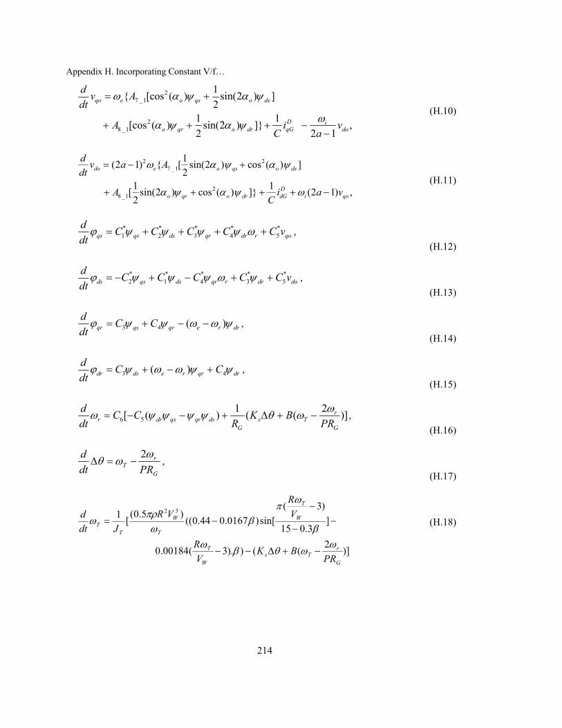
Appendix H. Incorporating Constant V/f…
214
27 _1
28 _1
1 [cos ( ) sin(2 ) ]2
1 1[cos ( ) sin(2 ) ] ,2 2 1
qo e o qs o ds
D io qr o dr qG do
d v Adt
A i vC a
ω α ψ α ψ
ωα ψ α ψ
= +
+ + + −−
(H.10)
2 27 _1
28 _1
1(2 1) [ sin(2 ) cos ( ) ]2
1 1[ sin(2 ) cos ( ) ] (2 1) ,2
do e o qs o ds
Do qr o dr dG i qo
d v a Adt
A i a vC
ω α ψ α ψ
α ψ α ψ ω
= − +
+ + + + −
(H.11)
* * * * *1 2 3 4 5qs qs ds qr dr r qo
d C C C C C vdtϕ ψ ψ ψ ψ ω= + + + + ,
(H.12)
* * * * *2 1 4 3 5ds qs ds qr r dr do
d C C C C C vdtϕ ψ ψ ψ ω ψ= − + − + + ,
(H.13)
3 4 ( )qr qs qr e r drd C Cdtϕ ψ ψ ω ω ψ= + − − ,
(H.14)
3 4( )dr ds e r qr drd C Cdtϕ ψ ω ω ψ ψ= + − + ,
(H.15)
6 51 2[ ( ) ( ( )]r
r dr qs qr ds s TG G
d C C K Bdt R PR
ωω ψ ψ ψ ψ θ ω= − − + ∆ + − ,
(H.16)
G
rT PRdt
d ωωθ 2−=∆ ,
(H.17)
)]2(()).3(00184.0
]3.015
)3(sin[)0167.044.0(()5.0([1 32
G
rTs
W
T
W
T
T
W
TT
PRBK
VR
VR
VRJdt
d
ωωθβωβ
ωπβ
ωπρ
ω
−+∆−−
−−
−−=
(H.18)

215
Appendix I Linearized Model Of the Wind Turbine System
I.1 Linearization the Nonlinear equations
The linearized equations based on the eleven nonlinear equations (H.8)-(H.18) are as follows:
0
0
00
2
1 cos( )2 1
2 (sin( ) )( )(2 1)
gridD D Di Gm VF oqG qG dG qo e
i i iD
i dG Gm VF o eo
i
d R V Ki i i vdt L a L L
i V Kaa L
ω α ω
ω α ω α
∆ = − ∆ − ∆ − ∆ + ∆−
+ ∆ − ∆−
, (I.1)
0
0 00
0
1(2 1)
sin( ) (cos( ) )2 ( )
D D DidG grid qG dG do
i i
DGm VF o Gm VF o ee grid qG
i i
d Ri a i i vdt L L
V K V Ki aL L
ω
α α ωω ω α
∆ = − ∆ − ∆ − ∆
− ∆ + ∆ − ∆, (I.2)
0
0
0 2
3,5 3,6 3,7
3,8 3,1 3,3
12 1
2(2 1)
gridDqo qG do
grid doe o
qs ds qr
dr
dv i v
dt C av
aa
a a a
a b b
ω
ωω α
ψ ψ ψ
ψ
∆ = ∆ − ∆−
+ ∆ + ∆ + ∆−
+ ∆ + ∆ + ∆
+ ∆, (I.3)
4,7 4,8
4,1 4,2 4,3
04,5 4,6
1 (2 1)do
e o
qs ds qr drDdG grid qo
dv
dta
a a
b b b
i a v a aC
ω α
ψ ψ ψ ψω∆ =
+ ∆ + ∆ + ∆
∆ + ∆ + ∆ + ∆∆ + − ∆ +, (I.4)
* * * * 01 2 3 4
* * 0 * 0 * 04 5 2 5( )
qs qs e ds qr g dr
odr g e qo ds qo e
d C C C Cdt
C C v C C v
ψ ψ ω ψ ψ ω ψ
ψ ω ω ψ ω
∆ = ∆ + ∆ + ∆ + ∆
+ ∆ + ∆ + + ∆, (I.5)
* * * 02 1 4
* * 0 * 0 * 0 * 03 5 4 2 5( )
ds e qs ds g qr
dr e do qr g qs do e
d C C Cdt
C C v C C C v
ψ ω ψ ψ ω ψ
ψ ω ψ ω ψ ω
= − ∆ + ∆ − ∆
+ ∆ + ∆ − ∆ + − + ∆, (I.6)

Appendix I. Linearized Model…
216
0 0 0 03 4qr qs qr e dr g dr dr g dr e
d C Cdt
ψ ψ ψ ω ψ ω ψ ψ ω ψ ω∆ = ∆ + ∆ − ∆ + ∆ + ∆ − ∆ , (I.7)
0 0 0 03 4( )dr ds e g qr dr qr g qr e
d C Cdt
ψ ψ ω ω ψ ψ ψ ω ψ ω∆ = ∆ + − ∆ + ∆ − ∆ + ∆ , (I.8)
9,5 9,6 9,7 9,8 2
9,1
2
( )
g qs ds qr dr gG gear
sT e
G gear G gear
d Ba a a adt PJ n
K B bJ n J n
ω ψ ψ ψ ψ ω
δθ ω ω
∆ = ∆ + ∆ + ∆ + ∆ − ∆
+ ∆ + ∆ + ∆, (I.9)
2( ) T ggear
ddt Pn
δθ ω ω∆ = ∆ − ∆ , (I.10)
7 5 11,4 11,511,11( )T g T Wd K K b V bdt
aω ω δθ ω β∆ = ∆ + ∆ + ∆ + ∆ + ∆ , (I.11)
where
001 )(
T
WVKω
= , )3)((3.015
00
02 −
−=
W
T
VRK ω
βπ
, 021
03 βKKK += , 0
004 3.015 β
π−
−= WVRK ,
006 WVK = , 0 0 0 2
7 1 6 0 2 01
0.3( ) ( 3)(15 0.3 )
RK K KK
πβ
= −−
,
2 0 0 2 03,5 7 _1 3,6 7 _1 3,7 8 _1
0 2 03,8 8 _1 4,5 7 _1
2 2 0 2 04,6 7 _1 4,7 8 _1
4,8 8 _1
1( cos ( )) , ( sin(2 )) , ( cos ( )) ,2
1 1( sin(2 )) , ((2 1) sin(2 )) ,2 2
1((2 1) cos ( )) , ((2 1) sin(2 )) ,2
(
e o e o e o
e o e o
e o e o
a A a A a A
a A a A a
a A a a A a
a A
ω α ω α ω α
ω α ω α
ω α ω α
= = =
= = −
= − = −
= 0 06 69,5 9,62 0 2 0
0 06 69,7 9,82 0 2 0
0 2 0 0 0 0 0 0 0 2 0 011,11 1 6 2 1 4 2 3 1 5 6 4 6
2 2 0 ,( ) ( )
,( ) ( )
( ( ) sin( ) cos( )) ( )
(2 1) cos ( )) , ,
,
,
dr qrG e G e
ds qsG e G e
e oC C
a aJ J
C Ca a
J J
a K K K K K K K K K K K K
a ψ ψω ω
ψ ψω ω
ω α −= =
= = −
= − − − +
−
* 2 * 2 03,1 7 8
* * 03,3 7 8
1 1 [cos ( ) sin(2 ) ] [cos ( ) sin(2 ) ] ,2 2
[ sin(2 ) cos(2 ) ] [ 2sin( ) cos(2 ) ] ,
o qs o ds o qr o dr
e o qs o ds o qr o dr
b A A
b A A
α ϕ α ψ α ψ α ψ
ω α ψ α ψ α ψ α ψ
= + + +
= − + + − +

Appendix I. Linearized Model…
217
2 * 2 * 2 04,1 7 8
* 2 * 2 04,2 7 8
2 *4,3 7
1 1(2 1) [ sin(2 ) cos ( ) ] [ sin(2 ) cos ( ) ] ,2 2
1 14(2 1) [ sin(2 ) cos ( ) ] [ sin(2 ) cos ( ) ] ,2 2
(2 1) [cos(2 ) sin(2 )
o qs o ds o qr o dr
e o qs o ds o qr o dr
e o qs o
b a A A
b a A A
b a A
α ψ α ψ α ψ α ψ
ω α ψ α ψ α ψ α ψ
ω α ψ α
= − + + +
= − + + +
= − − * 08
0 0 0 069,1 3 0
0 0 0 0 0 0 0 0 0 0 011,4 1 6 2 4 2 3 5 6 3 1 5 6 4
0 0 0 0 0 2 0 0 2 0 0 211,5 7 3 2 1 6 2 2 6 3 1 6 4
] [cos(2 ) cos(2 ) ] ,
2 ( ),( )
(3 sin( ) cos( )) 2 3 ,
cos( ) ( ) sin( ) ( ) ( ) .
ds o qr o dr
dr qs qr dse
A
Cb
b K K K K K K K K K K K K K
b K K K K K K K K K K K K
ψ α ψ α ψ
ψ ψ ψ ψω
+ −
= −
= + + +
= + + +
I.2 Output equations of the small-signal model
The output of small-signal model contains the grid real and reactive powers, i.e., ∆PGrid and
∆QGrid that can be derived based on the nonlinear equations (3.49) and (3.50), as follows:
0 0 00
00
3 cos( ) sin( ) (sin( ) cos( ) )2
1 (cos( ) sin( ) ) ,
D D D DGmGrid o qG o dG o qG o dG o
VF e
D Do qG o dG e
e
VP i i i iK
i i
α α α α αω
α α ωω
∆ = ∆ − ∆ − + ∆
− − ∆ (I.12)
0 0 0
0
00 0
3 1( ) sin( ) cos( )2 (2 1)
(cos( ) sin( ) )
2 1(sin( ) cos( ) ) ( ).(2 1)
D DGmGrid o qG o dG
VF eD D
o qG o dG o
D Do qG o dG e
e
VQ i iK a
i i
i i aa
α αω
α α α
α α ωω
∆ = − ∆ + ∆−
+ − ∆
−+ + ∆ − ∆
−
(I.13)

Appendix I. Linearized Model…
218
I.3 Numerical values of the Jacobian matrices
The numerical values of the Jacobian matrices A, B, C, and D at the operating point are:
A= -100 -628.32 -1000 0 0 0 0 0 0 0 0
226.19 -100 0 -1000 0 0 0 0 0 0 0
1e6 0 0 -628.32 -1.0479e5 0 1.025e5 0 0 0 0
0 1e6 226.19 0 0 -37726 0 36902 0 0 0
0 0 325.55 0 -45.54 -376.99 44.375 50.528 212.38 0 0
0 0 0 325.55 376.99 -45.54 -50.528 44.375 -14.612 0 0
0 0 0 0 28.905 0 -29.551 1.5489 1591.1 0 0
0 0 0 0 0 28.905 -1.5489 -29.551 -109.47 0 0
0 0 0 0 0.87472 -0.060182 -0.89748 0.014545 -1.0531 16849 42.123
0 0 0 0 0 0 0 0 -0.025 0 1
0 0 0 0 0 0 0 0 1.25 -20000 -55.302
B= 4331.6 5243.1 0 0 0
0 -6371.2 -9.798e5 0 0
22411 -4527.5 -7.9796e6 0 0
-7619.9 -1.792e7 3.0415e6 0 0
-222.94 0 0 0 0
24.59 0 0 0 0
-1591.1 0 0 0 0
109.47 0 0 0 0
0.39844 0 0 0 0
0 0 0 0 0
0 0 0 22.848 -5.3188
C=
9798 0 0 0 0 0 0 0 0 0 0 0 -16330 0 0 0 0 0 0 0 0 0 D=
219.62 0 -24528 0 0 108.44 1.3627e5 1.3799e5 0 0

219
Appendix J
Luenberger Observer Construction
The block diagram of the Luenberger observer is shown in Fig. J-1. The observer is fundamentally a
copy of the plant, so that it has the same input and almost the same differential equations. First, the
actual measured output y is compared to the estimated output ŷ, and then, using the observer gain L,
the estimated states x is produced so that this state vector tends to the actual state vector x .
-
yu
System
uDxCyuBxAx
+=+=
ˆ ˆ ˆ( )x A x Bu L y y= + + −
y
x
Observer
L
C
D
+
Fig. J-1: The closed-loop feedback system with optimal observer augmented
The observer state-space equations are as follows:
ˆ ˆ ˆ( ) ,ˆ ˆ .x Ax L y y Buy Cx Du= + − += +
(J.1)
The state-estimator or observer error is:
ˆe x x= − . (J.2)

Appendix J. Luenberger Observer
220
In general, the observer is called asymptotically stable if the observer error converges to zero, for any
initial condition e(0), when t→∞ [136]. For a Luenberger observer, one can prove that observer error
dynamics is [130][131]:
ˆ ( ) ( )e x x A LC e t= − = − . (J.3)
Therefore, the Luenberger observer is asymptotically stable if and only if the eigenvalues of A-LC
are all in the left-half plane. Moreover, arbitrary observer error dynamics can be assigned if and only
if (AT, CT) is controllable.
In practice, the methods such as pole placement or LQ can be used to find the observer gain L so
that the observer is asymptotically stable with desired dynamics. Since the observer dynamics should
be much faster than the system itself, we need the eigenvalues of A-LC to be farther to the left than
those of A-BK [130][131].
J-1 Closed-Loop Equations for the System Based on Observer
In this subsection, equations of the closed-loop system, comprised of the augmented system together
with the state feedback controller, Fig. 4-2, are modified to include the Luenberger observer
equations. The closed-loop observer-based state-feedback with integral control scheme is shown in
Fig. 4-14.
In this system, the controller contains the following three dynamics:
• The state-feedback equations using the estimated state x :
[ ]1 2 1 2
ˆ ˆˆ
x xu K K K K x K z
z z⎡ ⎤ ⎡ ⎤
= − = − = − −⎢ ⎥ ⎢ ⎥⎣ ⎦ ⎣ ⎦
. (J.4)
• The integrator equations:
rz y y= − . (J.5)
• The observer equations:
ˆ ˆ ˆ ˆ ˆ ˆ( ) ( ) ( )x Ax L y y BKx A BK x L y y= + − − = − + − , (J.6)
where ˆ ˆ( )y C DK x= − .

Appendix J. Luenberger Observer
221
Although the closed-loop system state vector is ˆ[ ]Tx z x , choosing the states representation
[ ]Tx z e is more practical in the implementation of the state-space model. Therefore, the state-
space equations are:
1 2 1( )x Ax Bu A BK x BK z BK e= + = − − + , (J.7)
1 2 1( ) ( ) ( )r rz y y C DK x DK z DK e y= − = − − + − , (J.8)
ˆ ( )e x x A LC e= − = − . (J.9)
Finally, the output equation is:
1 2 1( ) ( ) ( )y Cx Du C DK x DK z DK e= + = − − + . (J.10)
J-2 Optimal Observer
This subsection is dedicated to the use of LQ method to design an optimal observer. The system with
a Luenberger observer, equations (J.7)-(J.10), is considered. To use the LQ method to find an optimal
observer, the observer dynamic equation should be rewritten as an LQ problem to design the observer
gain L in an optimal way. One can prove that the observer error dynamics, equation (J.9), is the same
as that of the following fictitious error [130]:
T Tfic fic fice A e C u= + , (J.11)
Tfic ficu L e= − . (J.12)
Equations (J.11) and (J.12) are in the form of a fictitious system and controller; so, it is possible to
use the LQ method to design the optimal controller, and get the optimal gain LT for the system of
(J.11). To find the optimal controller, the following requirements should be satisfied:
• (AT,CT) is controllable (stabilizable)
• (Qfic,AT) is observable (detectable)

Appendix J. Luenberger Observer
222
where Qfic is the penalty weighting matrix of the fictitious error. As with the previous explanation for
the LQ method, the design of the optimal observer is possible by solving the corresponding ARE,
equation (4.6). Then, the observer gain L matrix can be calculated from the following formula:
1Tfic ficL P C R−= , (J.13)
where Pfic is a unique symmetrical positive semi-definite solution of the ARE, and Rfic the penalty
weighting matrix of the fictitious control signals.

223
Appendix K Transfer Function of the Wind Turbine System
11 12
21 22
( )G G
G sG G⎡ ⎤
= ⎢ ⎥⎣ ⎦
G11=
219.62 (s+1.935e5)(s+25.48)(s-0.08957) (s2+56.24s+2.042e4) (s2 +49.24s+6.833e4)(s2-90.57s+6.649e7)(s2+112.5s + 1.01e9)
________________________________________________________________________________________________________________
(s+25.24)(s2 + 24.41s+ 188)(s2 + 56.25s + 2.045e4)(s2 +101.8s+1.416e5) (s2+99.53s + 9.969e8) (s2 + 99.29s+1.05e9)
G12=
51371893.8(s+5.784e4)(s-5.613e4)(s-2003)(s+27.08)(s2+1.954s+14.44)(s2+56.24s+2.04e4)(s2 +2142s+2.829e6)
________________________________________________________________________________________________________________
(s+25.24) (s2 +24.41s+1188) (s2+56.25s+2.045e4) (s2+101.8s +1.416e5) (s2+99.53s +9.969e8) (s2 +99.29s +1.05e9)
G21=
108.44(s-4992)(s+1.084e4)(s-48.88)(s-6.062)(s+5.299)(s2 +56.19s +2.044e4) (s2-3726s+7.169e7)(s2-1718s + 7.597e8)
________________________________________________________________________________________________________________
(s+25.24) (s2+ 24.41s + 1188) (s2+56.25s+2.045e4) (s2+101.8s+1.416e5)(s2+99.53s+9.969e8) (s2+99.29s + 1.05e9)
G22=
136270 (s+3.413e4) (s-3.326e4) (s+25.71) (s2+24.55s +1193) (s2+56.25s+2.045e4) (s2+92.35s+1.417e5) (s2+99.19s+1.034e9)
________________________________________________________________________________________________________________
(s+25.24) (s2 + 24.41s +1188) (s2 + 56.25s + 2.045e4) (s2 + 101.8s + 1.416e5) (s2+99.53s + 9.969e8) (s2 + 99.29s + 1.05e9)

224
Appendix L Parameters of the system under study
Table L.1: Parameters of the small wind turbine system
Induction Generator [123] Wind Turbine System Matrix Converter Grid(Infinite Bus)
Vrated=400[V] JT=10 [kg.m2] Ri=Ro=0.0001[Ω] VG=400[V]
frated=60[Hz], P=6[Poles] ngear=20 Li=Lo=.01 [mH] fG=60[Hz]
rs=0.294, rr=0.156 [Ω] ρair =1.25[kg/m3] C=0.001[mF]
Ls=1.39, Lr=0.74 [mH], LM=41 [mH] R=10 [m] 0<q≤0.87
J=0.4[Kg.m2], Pmech_loss=1%Prated 0≤a≤1
Table L.2: Parameters of the system under study
Induction Generator [96] Wind Turbine System Matrix Converter Grid(Infinite Bus)
500[hp], 2.3[KV], 1773[rpm] JT=100 [kg.m2] Ri=Ro=0.1[Ω] VG=4[KV]*
TB=1.98×10³[N.m], IB(abc)=93.6[A] Ks=2×10⁶ [Nm/rad] Li=Lo=1 [mH] fG=60[Hz]
rs=0.262, rr=0.187 [Ω] B=5×10³ [Nm/rad/s] C=0.1[mF]
Xls=1.206, Xlr=1.206, XM=54.02 [Ω] ngear=20 0<q≤0.87
J=11.06[Kg.m2] ρair =1.25[kg/m3] 0≤a≤1
P=4[Poles], Pmech_loss=1%Prated R=10 [m]
*Note that the voltage rating has not been chosen based on the data of a practical wind turbine system.
High voltage levels make the size of the generator impractical due to the high insulation strength
requirements.

225
Bibliography
[1] BTM Consults internet homepage, available at http://www.btm.dk/, March 2007.
[2] CanWEA, Canadian wind energy association, available at www.canwea.ca/, February, 2007.
[3] Donna Cansfield (Ontario Energy Minister), Address of Onatrio’s Largest Wind Farm
Officially opens, , available at aimpowergren.com, April, 2006.
[4] L. Surugiu, and I. Paraschivoiu, "Environmental, social, and economical aspects of wind
energy," AIAA-2000-3008 Environmental, Social and Economical Aspects of Wind Energy, 35th
Intersociety, vol.2, pp. 1167-1174.
[5] S. Krohn, The wind energy pioneer - Poul la Cour, Published by The Danish Wind Turbine
Manufacturers Association, available at: http://webasp.ac-aix-marseille.fr/rsi/bilan/action_0405
/13LduRempart/Doc/Doc_page/windpower.pdf, February, 2008.
[6] R. Hoffmann and P. Mutschler, "The Influence of Control Strategies on the Energy Capture of
Wind Turbines, " Application of Electrical Energy, Piscataway, NJ, USA, 2000, pp. 886-893
[7] P. Migliore, J. van Dam, and A. Huskey, "Acoustic Tests of Small Wind Turbinesat," available
at http://www.wind.appstate.edu/reports/NRELAcousticTestsofSmallWindTurbines.pdf,
February, 2007.
[8] L. H. Hansen, L. Helle, F. Blaabjerg, E. Ritchie, S. Munk- Nielsen, H. Bindner, P. Sørensen,
and B. Bak-Jensen, "Conceptual survey of Generators and Power Electronics for Wind
Turbines, " Risø National Laboratory, Roskilde, Denmark December 2001.
[9] O. Carlson, J. Hylander, and K. Thorborg, "Survey of variable speed operation of wind
turbines," In European Union Wind Energy Conf., Goeteborg, Sweden, May 1996, pp. 406-
409.
[10] M. Idan, D. Lior, and G. Shaviv, "A robust controller for a novel variable speed wind turbine
transmission, " Journal of Solar Energy Engineering, November 1998, pp.120:247-252.
[11] S. Bhowmik and R. Spee, "Wind speed estimation based variable speed wind power
generation," Industrial Electronics Society, 1998. IECON '98, Proc. of the 24th Annual Conf.
of the IEEE , vol. 2, 31 Aug.-4 Sept. 1998 pp.596 – 601.

Bibliography
226
[12] M. G. Simoes, B. K. Bose, and R. J. Spiegel, "Fuzzy logic based intelligent control of a
variable speed cage machine wind generation system, " IEEE Tran. On Power Electronics,
vol.: 12, Issue: 1, pp. 87 – 95, Jan. 1997.
[13] Q. Wang and L. Chang, "An intelligent maximum power extraction algorithm for inverter-
based variable speed wind turbine systems, " IEEE Trans. Power Electronics, vol. 19, Issue: 5,
pp. 1242 – 1249, Sept. 2004.
[14] A. Miller, E. Muljadi, and D.S. Zinger, "A variable speed wind turbine power control," IEEE
Trans. on Energy Conversion, vol. 12, Issue: 2, pp. 181 – 186, June 1997.
[15] Xu Longya and C. Wei, "Torque and reactive power control of a doubly fed induction machine
by position sensorless scheme, " IEEE Trans. on Industry Applications, vol. 31, Issue 3, pp.
636 – 642, May-June 1995.
[16] W. Lu and B. T. Ooi, "Multiterminal LVDC system for optimal acquisition of power in wind-
farm using induction generators," IEEE Trans. On Power Electronics, vol. 17, NO. 4, pp. 558-
563, JULY 2002.
[17] J.L. Rodriguez-Amenedo, S. Arnalte, and J.C. Burgos, "Automatic generation control of a wind
farm with variable speed wind turbines," IEEE Trans. On Energy Conversion, vol 17, Issue 2,
pp. 279 – 284, June 2002.
[18] D. Seyoum and M.F. Rahman, "The dynamic characteristics of an isolated self-excited
induction generator driven by a wind turbine," Rec. in Proc. IAS Conf., Industry Applications
Conf., Annual Meeting, vol. 2, Oct. 2002, pp. 731 – 738.
[19] F. Blaabjerg, Zhe Chen, and S.B. Kjaer, "Power electronics as efficient interface in dispersed
power generation systems," IEEE Trans. on Power Electronics, vol. 19, Issue: 5 , pp.1184 –
1194, Sept. 2004.
[20] L.L. Freries, Wind Energy Conversion Systems , Prentice Hall,1990.
[21] S.Heier, Grid Integration of Wind Energy Conversion Systems, Chapter 1, John Wiley & Sons
Ltd, 1998.
[22] J.F. Manwell, J.G. McGowan, A.L. Rogers, Wind Energy Explained, Theory, Design and
Application, Wiley, 2002.
[23] S. Mathew, Wind Energy Fundamentals, Resource Analysis, and Economics, Springer, 2006.
[24] P.G. Casielles, J. Sanz, and J. Pascual, "Control system for a wind turbine driven self excited
asynchronous generator," in Proc. Mediterranean Electrotechnical Integrating Research,

Bibliography
227
Industry and Education in Energy and Communication Engineering, MELECON '89 Conf.,
April 1989, pp. 95 – 98.
[25] D.A. Torrey, "Variable-reluctance generators in wind-energy systems, " Rec. in IEEE PESC
'93, Power Electronics Specialists Conf., June 1993, pp. 561 – 567.
[26] J. Matevosyan, Wind power in areas with limited export capability, Licentiate Thesis Royal
Institute of Technology Department of Electrical Engineering Stockholm, 2004.
[27] A.J.G. Westlake, J.R. Bumby, and E. Spooner, "Damping the power-angle oscillations of a
permanent-magnet synchronous generator with particular reference to wind turbine
applications," in IEE Proc. Electric Power Applications, vol. 143, Issue: 3, May 1996, pp. 269–
280.
[28] S. Grabic, N. Celanovic, V. Katie, "Series converter stabilized wind turbine with permanent
magnet synchronous generator," in IEEE Conf. PESC 04, Power Electronics Specialists
Conference, vol. 1, June 2004, pp. 464 – 468.
[29] L. Dambrosio, and B. Fortunato, "One step ahead adaptive control technique for a wind
turbine-synchronous generator system," in Proc. IECEC-97, Intersociety Energy Conversion
Engineering Conference, vol. 3, July 1997, pp. 1970 – 1975.
[30] D.S .Zinger, E. Muljadi, "Annualized wind energy improvement using variable speeds," IEEE
Trans. on Industry Applications , vol. 33 , Issue: 6 , pp. 1444 – 1447 Nov.-Dec. 1997.
[31] P. Bauer, S.W.H. De Haan, and M.R.Dubois, "Wind energy and Offshore Windparks: State of
the Art and Trends," EPE-PEMC Dubrovnik & Cavat, 2002, pp 1-15.
[32] P. Bauer, S.W.H. De Haan, C.R. Meyl, and J.T.G. Pierik, "Evaluation of electrical systems for
offshore wind farms," Rec. in IEEE Industry Applications Conf., vol.3, Oct. 2000, pp. 1416–
1423.
[33] E. Bogalecka and Z. Krzeminski, "Control systems of doubly-fed induction machine supplied
by current controlled voltage source inverter, " in Sixth International Conf. on Electrical
Machines and Drives, Conf. Publ. No. 376, Sep 1993, pp. 168 – 172.
[34] C. Knowles-Spittle, B.A.T. Al Zahawi, and N.D. MacIsaac, "Simulation and analysis of 1.4
MW static Scherbius drive with sinusoidal current converters in the rotor circuit," in Proc. IEE
Seventh International Conf. on Power Electronics and Variable Speed Drives, Conf. Publ. No.
456, Sept. 1998, pp. 617 – 621.

Bibliography
228
[35] R. Pena, J.C. Clare, and G.M. Asher, "A doubly fed induction generator using back-to-back
PWM converters supplying an isolated load from a variable speed wind turbine, " Electric
Power Applications, IEE Proc., vol. 143, Issue: 5, Sept. 1996, pp. 380 – 387.
[36] T. Yifan and Xu Longya, " A flexible active and reactive power control strategy for a variable
speed constant frequency generating system," IEEE Trans. on Power Electronics, vol. 10 ,
Issue: 4 , pp. 472 – 478, July 1995.
[37] Wen-Song Chienand and Ying-Yu Tzou, "Analysis and design on the reduction of DC-link
electrolytic capacitor for AC/DC/AC converter applied to AC motor drives, " in Proc. IEEE
PESC 98, Power Electronics Specialists Conf., vol. 1, May 1998, pp. 275 – 279.
[38] J.S. Kim and S. K., Sul, "New control scheme for AC-DC-AC converter without DC link
electrolytic capacitor, " in IEEE Proc. PESC '93, Power Electronics Specialists Conference,
1993, June 1993, pp. 300 – 306.
[39] K. Siyoung, S. Seung-Ki, and T.A. Lipo, "AC to AC power conversion based on matrix
converter topology with unidirectional switches," in Proc. APEC '98, Applied Power
Electronics Conf. and Exposition, 1998, vol. 1, Feb. 1998, pp. 301 – 307.
[40] M. Salo and H. Tuusa, "A high performance PWM current source inverter fed induction motor
drive with a novel motor current control method," in Proc. IEEE PESC 99, Power Electronics
Specialists Conference, 1999, vol. 1 , 27 June-1 July 1999, pp. 506 – 511.
[41] M. Venturini, "A new sine wave in sine wave out, conversion technique which eliminates
reactive elements, " in Proc. POWERCON 7, 1980, pp. E3_1–E3_15.
[42] M. Venturini and A. Alesina, "The generalized transformer: A new bidirectional sinusoidal
waveform frequency converter with continuously adjustable input power factor, " in Proc.
IEEE PESC’80, 1980, pp. 242–252.
[43] J. Rodriguez, "A new control technique for AC–AC converters," in Proc IFAC Control in
Power Electronics and Electrical Drives Conf., Lausanne, Switzerland, 1983, pp. 203–208.
[44] D.H. Shin, G.-H. Cho, and S.-B. Park, "Improved PWM method of forced commutated
cycloconvertors, " in IEE Proc. Electric Power Applications, Proc. B, vol. 136, Issue 3, May
1989, pp.121 – 126.
[45] Y. H. Kim and M. Ehsani, "Control of force-commutated direct frequency changers," in Conf.
Industry Applications, 1990, pp. 1163 – 1170.
[46] N. Burany, "Safe control of four-quadrant switches," in Conf. Rec. Industry Applications, Oct.
1989, pp.1190 – 1194.

Bibliography
229
[47] L. Huber, D. Borojevic, and N. Burany, "Electric Analysis, design and implementation of the
space-vector modulator for forced-commutated cycloconvertors," in Proc. B, IEE Power
Applications, vol. 139, Issue 2, March 1992, pp. 103 – 113.
[48] M. Ziegler and W. Hofmann, "Semi natural two steps commutation strategy for matrix
converters," Rec. 29th Annual Power Electronics Specialists IEEE Conf., PESC 98, vol. 1,
May 1998, pp. 727 – 731.
[49] R. Teichmann and j. Oyama, "ARCP soft-switching technique in matrix converters," IEEE
Trans. On Industrial Electronics, vol. 49, Issue 2, pp. 353 – 361, April 2002.
[50] J. Rodriguez, "A new control technique for AC–AC converters," in Proc. IFAC Control in
Power Electronics and Electrical Drives Conf., Lausanne, Switzerland, 1983, pp. 203–208.
[51] J. Oyama, T. Higuchi, E. Yamada, T. Koga, and T. Lipo, "New control strategy for matrix
converter, " in Proc. IEEE PESC’89, 1989, pp. 360–367.
[52] P. D. Ziogas, S. I. Khan, and M. H. Rashid, "Analysis and design of forced commutated
cycloconverter structures with improved transfer characteristics, " IEEE Trans. Ind.
Electronics, vol. IE-33, pp. 271–280, Aug. 1986.
[53] P. Ziogas, S. Khan, and M. Rashid, "Some improved forced commutated cycloconverter
structures, " IEEE Trans. Ind. Applicat., vol. 1A-21, pp. 1242–1253, Sept./Oct. 1985.
[54] A. Alesina and M. G. B. Venturini, "Analysis and design of optimum amplitude nine-switch
direct AC–AC converters, " IEEE Trans. Power Electron., vol. 4, pp. 101–112, Jan. 1989.
[55] L. Huber and D. Borojevic, "Space vector modulated three phase to three phase matrix
converter with input power factor correction," IEEE Trans. Ind. Applicat., vol. 31, pp. 1234–
1246, Nov./Dec. 1995.
[56] H. Hotate and K. Masuse, "Basic characteristics of matrix-converter-controlled by space vector
modulation considering input voltage conditions" in Conf. IPEMC 2004, the 4th International
Power Electronics and Motion Control, vol. 2, Aug. 2004 pp. 719 – 723.
[57] C. Wang and Q. Lu, "Analysis of naturally sampled space vector modulation PWM in over
modulation region," in Conf. IPEMC 2004, the 4th International Power Electronics and
Motion Control Conf., vol. 2, Aug. 2004, pp. 694 – 698.
[58] L. Wei, T.A. Lipo, "A novel matrix converter topology with simple commutation," Rec. in
Conf. Thirty-Sixth IAS 2001, Industry Applications IEEE Conference Annual Meeting, vol.
3, Sept. 2001, pp. 1749 – 1754.

Bibliography
230
[59] Lixiang Wei, T.A. Lipo, Ho Chan, "Matrix converter topologies with reduced number of
switches," In Conf. PESC02, Power Electronics Specialists Conference, vol. 1, June 2002, pp.
57 – 63.
[60] P.W. Wheeler, J. Rodriguez, J. C. Clare, L. Empringham, A. Weinstein, "Matrix converters: a
technology review, " IEEE Trans. on Industrial Electronics vol. 49, Issue 2, pp. 276 - 288
April 2002
[61] C. Klumpner, P. Nielsen, I. Boldea, F. Blaabjerg, "A new matrix converter motor (MCM) for
industry applications," IEEE Trans. on Industrial Electronics, vol. 49, Issue 2, pp. 325-335.
April 2002
[62] D. Casadei, G. Serra, A. Tani, and L. Zarri, "Matrix converter modulation strategies: A new
general approach based on space-vector representation of the switch state," IEEE Trans. On
Industrial Electronics, vol. 49, pp. 370–381, Apr. 2002.
[63] O. Simon, J. Mahlein, M. N. Muenzer, and M. Bruckmarm, " Modern solutions for industrial
matrix-converter applications," IEEE Trans. On Industrial Electronics, vol. 49, Issue 2, pp.
401-406, April 2002
[64] L. Wei, Y. Matsushita, and T.A. Lipo, " Investigation of dual-bridge matrix converter operating
under unbalanced source voltages," in Conf. PESC '03, Power Electronics Specialist Conf., vol.
3, June 2003, pp. 1293 – 1298.
[65] F. Blaabjerg, D. Casadei, C. Klumpner, and M. Matteini, "Comparison of two current
modulation strategies for matrix converters under unbalanced input voltage conditions," IEEE
Trans. on Industrial Electronics, vol. 49, Issue 2, pp :289 – 296, April 2002.
[66] P.W. Wheeler, J.C. Clare, M. Apap, L. Empringham, C. Whitley, and G. Towers, "Power
supply loss ride-through and device voltage drop compensation in a matrix converter
permanent magnet motor drive for an aircraft actuator" in Conf. PESC 04, Power Electronics
Specialists Conf., vol. 1, June 2004, pp.149 – 154.
[67] C. Klumpner, and F. Blaabjerg, "Experimental evaluation of ride-through capabilities for a
matrix converter under short power interruptions," IEEE Tran. on Industrial Electronics, vol.
49, Issue 2, pp. 315 – 324, April 2002.
[68] J. Adamek, W. Hofmann, and M. Ziegler, "Fast commutation process and demand of
bidirectional switches in matrix converters, " in Conf. PESC '03, Power Electronics Specialist
Conf. vol. 3, June 2003, pp. 1281 – 1286.

Bibliography
231
[69] R. Sittig, A. Krysiak, and St. Chmielus, "Monolithic bidirectional switches promise superior
characteristics, " in Conf. PESC 04, Power Electronics Specialists Conference, vol. 4, June
2004, pp. 2977 – 2982.
[70] Kang Jun-Koo, H. Hara, E. Yamamoto, E. Watanabe, and J. Oyama, "Input harmonics
damping for high power quality applications of matrix converter," Rec. in 38th IAS Annual
Meeting, Industry Applications Conf., vol. 3, Oct. 2003, pp. 1498 – 1503.
[71] S. Ferreira Pinto, and J. Fernando Silva, "Input filter design for sliding mode controlled matrix
converters," in Conf. PESC ’01, Power Electronics Specialists Conference, vol. 2, June 2001,
pp. 648 – 653.
[72] D. Casadei, G. Serra, A. Tani, and L. Zarri, "Effects of input voltage measurement on stability
of matrix converter drive system," in Proc. IEE Electric Power Applications, vol. 151, Issue 4,
July 2004, pp. 487 – 497.
[73] D. Casadei, G. Serra, A. Tani, L. Zarri, "Stability analysis of electrical drives fed by matrix
converters, " in Proc. IEEE ISIE 2002, International Symposium on Industrial Electronics, vol.
4, July 2002, pp. 1108 – 1113.
[74] L. Helle, K.B. Larsen, A. H. Jorgensen, S. Munk-Nielsen, F. Blaabjerg, "Evaluation of
modulation schemes for three-phase to three-phase matrix converters," IEEE Transactions on
Industrial Electronics, vol. 51, issue 1, Feb. 2004 pp.158 – 171.
[75] M. Aten, C. Whitley, G. Towers, P. Wheeler, J. Clare, K. Bradley, "Dynamic performance of a
matrix converter driven electro-mechanical actuator for an aircraft rudder," in Proc. second
International Conference on Power Electronics, Machines and Drives, PEMD 2004, vol. 1,
April 2004, pp. 326 – 331.
[76] B. Ooi and M. Kazerani, "Elimination of the waveform distortions in the voltage-source-
converter type matrix converter," in Conf. Rec. IEEE-IAS Annu. Meeting, vol. 3, 1995, pp.
2500–2504.
[77] P. Nielsen, The matrix converter for an induction motor drive, Ph.D. dissertation, Inst. Energy
Technol., Aalborg Univ., Aalborg East, Denmark, 1996.
[78] P. W. Wheeler and D. A. Grant, "A low loss matrix converter for AC variable-speed drives," in
Proc. EPE Conf., vol. 5, 1993, pp. 27–32.
[79] A.M. Hava, R. J. Kerkman, T.A. Lipo, "A high performance generalized discontinuous PWM
algorithm, " in Proc. PEC’97, vol. 2, 1997, pp. 886–894.

Bibliography
232
[80] P. Nielsen, F. Blaabjerg, and J. K. Pedersen, "Space vector modulated matrix converter with
minimized number of switchings and a feed forward compensation of input voltage unbalance,
" in Proc. PEDES’96, vol. 2, 1996, pp. 833–839.
[81] J.Wu, P.Dong, J.M. Yang, and Y.R. Chen, "A Novel Model of Wind Energy Conversion
System," in Proc. DRPT2004, IEEE International Conf. on Electric Utility Deregulation and
Power Technologies , April 2004 Hong Kong, pp. 804-809.
[82] R., Teodorescu and F. Blaabjerg, "Flexible control of small wind turbines with grid failure
detection operating in stand-alone and grid-connected mode," IEEE Trans. on Power
Electronics vol. 19, Issue 5, pp. 1323 – 1332, Sept. 2004.
[83] T. Satish, K. K. Mohapatra, N. Mohan, "Speed Sensor-less Direct Power Control of a Matrix
Converter Fed Induction Generator for Variable Speed Wind Turbines," in Proc. Power
Electronics, Drives and Energy Systems, PEDES’06, Dec 2006, pp. 1-6.
[84] S. F. Pinto, L. Aparicio, P. Esteves, "Direct Controlled Matrix Converters in Variable Speed
Wind Energy Generation Systems Power Engineering," in Proc. Energy and Electrical Drives,
POWERENG 2007, April 2007, pp. 654 – 659.
[85] Huang Keyuan, He Yikang, "Investigation of a matrix converter-excited brushless doubly-fed
machine wind-power generation system," in Proc. Power Electronics and Drive Systems,
PEDS 2003, Nov. 2003, Vol. 1, pp. 743 – 748.
[86] Qi Wang, Xiaohu Chen, Yanchao Ji, "Control for Maximal Wind Energy Tracing in Matrix
Converter AC Excited Brushless Doubly-Fed Wind Power Generation System," in Proc. IEEE
Industrial Electronics, IECON 2006, Nov. 2006, pp. 718 – 723.
[87] L. Zhang, C. Watthanasarn, "A matrix converter excited doubly-fed induction machine as a
wind power generator," in Proc. Power Electronics and Variable Speed Drives, Sept. 1998, pp.
532 – 537.
[88] D. Aouzellag, K. Ghedamsi, E.M. Berkouk, "Network Power Flow Control of Variable Speed
Wind Turbine," in Proc. Power Engineering, Energy and Electrical Drives, POWERENG
2007, April 2007, pp. 435 – 439.
[89] L. Zhang, C. Watthanasarn, W. Shepherd, "Application of a matrix converter for the power
control of a variable-speed wind-turbine driving a doubly-fed induction generator," in Proc.
Industrial Electronics, Control and Instrumentation, IECON 97. Vol. 2, Nov. 1997, pp. 906-
911.

Bibliography
233
[90] M. Kazerani, Dynamic Matrix Converter Theory Development and Application, Ph.D. thesis,
Department of Electrical Eng., McGill University, Canada, 1995.
[91] B.T. Ooi and M. Kazerani, "Application of dyadic matrix converter theory in conceptual design
of dual field vector and displacement factor controls", in Proc. IEEE Industry Applications
Society Annual Meeting, Vol. 2, Oct. 1994, pp. 903-910.
[92] H. Nikkhajoei, A. Tabesh, and R. Iravani, "Dynamic model of a matrix converter for controller
design and system studies", IEEE Trans. on Power Delivery, Vol. 21, Issue 2, Apr. 2006, pp.
744 – 754.
[93] A. Alesina and M. Venturini, "Solid-state power conversion: A Fourier analysis approach to
generalized transformer synthesis", IEEE Trans. on Circuits and Systems, Vol. 28, Issue 4,
Apr. 1981, pp. 319 – 330.
[94] S.M. Barakati, M. Kazerani, J.D. Aplevich, "An overall model for a matrix converter,"
Accepted in IEEE International symposium on Industrial Electronics, ISIE08, June 2008, pp.
[95] S. M. Barakati, M. Kazerani, and J.D. Aplevich "A Dynamic Model for a Wind Turbine
System Including a Matrix Converter, " in Proc. IASTED, PES2007, January 2006, pp. 1-8.
[96] P. C. Krause, O Wasynczuk , S. D. Sudhoff, Analysis of electric machinery, IEEE Press, 1994.
[97] L. Neft and C.D. Shauder, "Theory and Design of a 30-hp Matrix converter, " IEEE Trans. on
Industrial Applications, vol. 28, no. 3, pp. 546-551, 1992.
[98] P. Wheeler and D. Grant, "Optimized input filter design and low loss switching techniques for
a practical matrix converter" in Proc. of industrial electronics, vol. 144, no. 1, Jan. 1997, pp.
53–60.
[99] D.G. Holmes and T.A. Lipo, "Implementation of a controlled rectifier using AC-AC matrix
converter theory", in Conf. Rec. PESC '89, Power Electronics Specialists Conf., June 1989,
vol.1, pp. 353 – 359.
[100] H.W. van der Broeck, H.-C. Skudelny, and G.V.Stanke, "Analysis and realization of a
pulsewidth modulator based on voltage space vectors," IEEE Tran. on Industry
Applications, vol. 24, pp: 142 – 150, Jan.-Feb. 1988.
[101] J.Hltz, "Pulsewidth modulation- A survey," IEEE Trans. on Industrial Electronics, vol.39, No.
5, 1999, pp. 410-420.
[102] L. Zhang, C. Wathanasarn, and W. Shepherd, "Switch sequencer circuit for safe commutation
of a matrix converter," Electronics Letters , vol. 31, Issue: 18 , Aug. 1995, pp. 1530 -1532.

Bibliography
234
[103] S. Kim, S-K. Sul and T.A. Lipo, "AC/AC power conversion based on matrix converter
topology with unidirectional switches, " IEEE Tran. on Industry Applications, vol .36, No. 1,
2000 , pp. 139-145.
[104] K. Iimori, K. Shinohara, O. Tarumi, Z. Fu, and M. Muroya, "New current-controlled PWM
rectifier-voltage source inverter without DC link components" in Proc. of the Power
Conversion Conf., Nagaoka, Japan, vol. II, Aug. 1997, pp. 783-786.
[105] J.W. Kolar, M. Baumann, F. Schafmeister, and H. Ertl, "Novel three-phase AC-DC-AC sparse
matrix converter," in Proc. Applied Power Electronics Conf. and Exposition, vol. 2, March
2002, pp. 777–791.
[106] S.M. Barakati, M. Kazerani, and X. Chen "A New Wind Turbine Generation System Based on
Matrix Converter, " in Proc. IEEE PES General Meeting, June 2005, pp. 2083-2089.
[107] E.S. Adin and W. Xu, "Control Design and Dynamic Performance Analysis of a Wind
Turbine-Induction Genrator Unit," IEEE Trans. On Energy Conversion, Vol. 15, NO. 1,
MARCH 2000, pp 91-96.
[108] J.G. Slootweg, H. Polinder, and W.L. Kling, "Representing Wind Turbine Electrical
Generating Systems in Fundamental Frequency Simulations," IEEE Trans. on Energy
Conversion, Vol. 18, No.4, Dec. 2003, pp 516-524.
[109] J. G. Slootweg, S. W. H. de Haan, H. Polinder, and W. L. Kling, "General Model for
Representing Variable Speed Wind Turbines in Power System Dynamics Simulations", IEEE
Trans. On Power Systems, Vol. 18, NO. 1, FEB.2003, pp. 144-151.
[110] L.S.T. Ackermann, "Wind Energy Technology and current status. A Review", Renewable and
Sustainable Energy Review, 4:315-375, 2000.
[111] E. Muljadi, C.P. Butterfield, "Power Quality Aspects in a Wind Power Plant," IEEE Power
Engineering Society General Meeting Montreal, Quebec, Canada June, 2006, pp.
[112] Rolf Grünbaum, "Voltage and power quality control in wind power" ABB Power Systems AB
available at http://library.abb.com/GLOBAL/SCOT/scot221.nsf/VerityDisplay/6B5A44E46B
AD5D3DC1256FDA003B4D11/$File/PowerGenEurope2001.pdf,February 2008.
[113] Tomas Petru and T. Thiringer, " Modeling of Wind Turbines for Power System Studies," IEEE
Trans. On Power System, Vol. 17, NO. 4, NOV. 2002,pp 1132-1139.
[114] A. D. Hansen, C. Jauch, P. Sørensen, F. Iov, F. Blaabjerg, "Dynamic wind turbine models in
power system simulation tool DIgSILENT," Risø National Laboratory, Roskilde, available at
http://www.digsilent.de/Software/Application_Examples/ris-r-1400.pdf, Dec. 2003.
Bibliography
235
[115] S. Seman, F. Iov, J. Niiranen, A. Arkkio, "Comparison of Simulators for Variable Speed Wind
Turbine Transient Analysis," International Journal of Energy Research, 2006, Vol. 30, Issue 9,
pp. 713-728.
[116] L. Mihet-Popa, F. Blaabjerg, and I. Boldea, "Wind turbine Generator modeling and Simulation
where rotational speed is the controlled variable," IEEE Trans. on Industry Application, Vol.
40, Jan/Feb 2004, pp 3-10.
[117] B. K. Bose, Power Electronics And Ac Drives, Prentice-Hall, 1986.
[118] P. C. Krause, Analysis of Electrical Machinery, McGraw-Hill Book Co, 1987.
[119] T.F. Chan, and Loi Lei Lai, "Capacitance requirements of a three-phase induction generator
self-excited with a single capacitance and supplying a single-phase load, " IEEE Trans. on
Energy Conversion, vol. 17, Issue 1, pp. 90 – 94, March 2002.
[120] Electric Systems Consulting ABB Inc., "Integration of Wind Energy into the Alberta Electric
System – Stages 2 & 3: Planning and Interconnection Criteria," Prepared for Alberta Electric
System Operator Report Number: 2004-10803-2.R01.4.
[121] B. Ozpineci, L.M. Tolbert, "Simulink implementation of induction machine model- a modular
approach", in Proc. Electric Machines and Drives Conference, IEMDC'03, Vol. 2, Jun. 2003,
pp. 728-734.
[122] A. Munoz-Garcıa, T. A. Lipo, and D. W. Novotny, "A New Induction Motor V/f Control
Method Capable of High-Performance Regulation at Low Speeds," IEEE Tran. on Industry
Applications, Vol. 34, NO. 4, July 1998 pp 813-821.
[123] Powersim Technologies inc, Psim User Manual, Version 4.1, Set.1999, available at
http://www.powersimtech.com, February, 2008.
[124] P. M. Anderson and A. Bose, "Stability Simulation of Wind Turbine Systems," IEEE Trans.
Power Apparatus and system , Vol. PAS-102, No. 12, pp. 3791-3795, Dec 1983.
[125] C. Nichita, D. Luca, B. Dakyo, E. Ceanga, " Large band simulation of the wind speed for real
time wind turbine simulators", IEEE Trans. on Energy Conversion, Vol. 17, No. 4, Dec. 2002,
pp 523 – 529.
[126] Starting (and Stopping) a Turbine, available at http://www.windpower.org/en/tour/wtrb
/electric.htm, February, 2008.
[127] J. D. Aplevich, The Essentials of Linear State-Space Systems, New York: Wiley, 1999.
[128] Khalil, H. Nonlinear Systems, Prentice Hall Inc, second edition, 1996.

Bibliography
236
[129] Jong-Yeob Shin, "Quasi-Linear Parameter Varying Representation of General Aircraft
Dynamic Over A Non-Trim Region", National Institute of Aerospace Hampton, Virginia,
NASA Report, 2007, NO.2005-08.
[130] D. Davison, Multivariable Control Systems, Course Notes-Part B, Published by University of
Waterloo, 2005.
[131] Control System Toolbox for Use with Matlab, Reference Version 6, available at
www.mathworks.com, February, 2008.
[132] B.C. Moore, "Principal component analysis in linear systems controllability, observability, and
model reduction", IEEE Transactions on Automatic Control, Vol. AC-26, (no. I), pages 17-32,
February 1981.
[133] Control tutorials for Matlab, University of Michigan, available at http://www.engin.umich.edu
/group/ctm/examples/pitch/SSpitch.html, February 2008.
[134] Joao P. Hespanha, LQG/LQR Controller Design, Lecture Note of ECE147C, University of
California, Santa Barbara, May 2006.
[135] D. Davison, "Feedback Control: Limitations on Tracking Performance," Presented in
graduated student talks seminar, ECE department at university of Waterloo, January 2007.
[136] Wikipedia, Typical Observer Model, available at http://en.wikipedia.org/wiki/State_observer,
February, 2008.
[137] Matlab Robust Control Toolbox, Reference Version 6, available at www.mathworks.com,
February, 2008.
[138] J. Medanic, H.S. Trap and W.R. Pekins, "Pole placement by performance criterion
modification," IEEE Transaction on Automatic Control, Vol. 33, No. 5, May 1988, pp. 596-
472.
[139] L. S. Shieh, H. M. Did and R. E. Yates, "Sequential Design of linear quadratic state regulator
via the optimal root-locus techniques," Control Theory and Applications, IEE proceedings,
1988, pp.289-294.
[140] K. Sugimoto, "Partial pole placement by LQ regulators: An inverse problem approach," IEEE
Transaction on Automatic Control, Vol. 43, No. 5, May 1998, pp. 706-708.
[141] D. Di Ruscio, "On the location of LQ-optimal closed-loop poles," Proceedings of the 30th
Conference on Decision and Control, 1991, pp. 2317-2320.
[142] M. H. Hsueh and H. Sehitoglu, "A new eigenvalue placement method for linear dynamic
systems," Proceedings of the 36th Conference on Decision and Control, 1997, pp. 4286-4287.

Bibliography
237
[143] D. A. Coly, "An introduction to genetic algorithms for scientists and engineers," Word
scientific, 1999.
[144] D.E. Gol, Genetic algorithms in search optimization and machine learning, Addison Wesle,
1989.
[145] N. Mansouri, H. Khaloozadeh, "The GA approach to eigenvalue placement of an LQ optimal
system," Proceedings of the 2002 IEEE International Conference on Artificial Intelligence
System, 2002, pp.
[146] Blight, J.D., Dailey, R.L. and Gangsass, D. (1994), "Practical control law design for aircraft
using multivariable techniques," International Journal of Control, Vol. 59, No. 1, 93-137.
[147] S. Skogestad, I. Postlethwaite, Multivariable feedback control analysis and design, Second
edition, Wiley, 2005.
[148] J. Lunze, Feedback control of large-scale systems, Prentice Hall, 1992.
[149] G. Zames and D. Bensoussan," Multivariable feedback, sensitivity and decentralized control,"
IEEE Transactions on automatic control, AC-28 (11), 1983, pp 1030-1035.
[150] J.M. Maciejowski, "Multivariable feedback design," Addison-Wesley Publishing Company,
1989.
[151] G.F. Franklin, J.D. Powell, A. Emami-Naeini, Feedback Control of Dynamic System, Fourth
Edition, Prentice-Hall, 2002.
[152] S. M. Barakati, J.D. Aplevich, M. Kazerani, "Controller Design for a Wind Turbine System
Including a Matrix Converter, " in Proc. IEEE Power Engineering Society General Meeting,
2007, pp 1- 8.
[153] T. Thiringer and J. Linders, "Control by variable rotor speed of a fixed-pitch wind turbine
operating in a wide speed range," IEEE Trans. Energy Conv.,vol. EC-8,pp.520-526,Sept. 1993.
[154] Q. Wang and L. Chang, "An intelligent maximum power extraction algorithm for inverter-
based variable speed wind turbine systems, " IEEE Trans. Power Electronics, vol. 19, Issue: 5,
pp. 1242 – 1249, Sept. 2004.
[155] E. Koutroulis, K. Kalaitzakis, "Design of a maximum power tracking system for wind-energy-
conversion," applications Industrial Electronics, IEEE Transactions on, Vol. 53, Issue 2,
April 2006 pp. 486 – 494.
[156] C. Hua and C. Shen, "Comparative study of Peak Power Tracking Techniques for Solar Storage
System," Applied power Electronics Conference and Exposition, vol.2,pp.679-685,Feb.1998.

Bibliography
238
[157] E. Koutroulis, K. Kalaitzakis, and N.C. Voulgaris, "Development of a microcontroller-based,
photovoltaic maximum power point tracking control system," IEEE Trans. on Power
Electronics vol. 16, Issue 1, pp. 46 – 54, Jan. 2001.
[158] T. Tanaka, T. Toumiya, "Output Control by Hill-Climbing Method For a Small Wind Power
Generating System, " Renewable Energy, Vol. 12, No. 4, 1977, pp. 387-400.
[159] I.K. Buehring, L.L. Freris, "Control Policies for Wind Energy Conversion Systems," IEE Proc.
, Vol. 128, pt. C, No. 5, Sept. 1981.
[160] M.Ermis, H.B. Ertan, E. Akpinar, F. Ulgut, Electric, "Autonomous wind energy conversion
system with a simple controller for maximum-power transfer," Power Applications, IEE
Proceedings B, Vol. 139, Issue 5, Sept. 1992, pp.421 – 428.
[161] R.J Wai, C.Y. Lin,Y.R. Chang, "Novel maximum-power-extraction algorithm for PMSG wind
generation system, Electric Power Applications," IET, Vol.1, Issue 2, March 2007, pp:275–
283.
[162] R. Chedid, F. Mard, and M. Basma, “Intelligent control of a class of wind energy conversion
system,” IEEE Trans. Energy Conv., vol. EC-14,pp.1597-1604, Dec. 1999.
[163] G. Poddar, A. Joseph, and A.K. Unnikrishnan, " Sensorless variable-speed controller for
existing fixed-speed wind power generator with unity-power-factor opration", IEEE Trans.
Industrial Electronics, vol.50, N0.5, pp.1007-1015, Oct. 2003.
[164] T. Senjyu, Y. Ochi, E. Muhando, N. Urasaki, H. Sekine, "Speed and Position Sensor-less
Maximum Power Point Tracking Control for Wind Generation System with Squirrel Cage
Induction Generator, " IEEE PES, PSCE '06. Oct. 29 2006-Nov. 1 2006, pp. 2038 – 2043.
[165] S.M. Barakati, M. Kazerani, and J.D. Aplevich, "A Mechanical Speed-Sensorless Maximum
Power Tracking Control for a Wind Turbine System Including a Matrix Converter, " accepted
in IEEE PES General Meeting,PES 2008.