Embed Size (px)
Citation preview
Modeling and Analysis of Three-Stage TransferLines with Unreliable Machines and Finite
BuffersSTANLEY B. GERSHWIN
Massachusetts Institute of Technology, Cambridge. Massachusetts
IRVIN C. SCHICKScientific Systems, Inc.. Cambridge, Massachusetts
(Received April 1980; accepted April 1982)
In an important ctass of systems, which arises in manufacturing, chemicalprocess, and computer contexts, objects move sequentially from one workstation to another, and rest between stations in buffers. In the manufacturingcontext, such systems are called transfer lines. The dynamic behavior of abuffered transfer tine with unreliable work stations is modeled as a Markovchain. The system states consist of the operationai conditions of the workstations and the levels of material in the butters. Ttie steady-state probabilitiesof these states are sought in order to establish relationships between systemparameters and performance measures such as production rate (efficiency),forced-down times, and expected in-process inventory. The steady stateprobabilities are found by choosing a sum-of-products form solution for aclass of states, and deriving the remaining expressions by using the transitionequations. In this way, the order of the system of equations to be solved isdrastically reduced. This algorithm suggests a general approach for solvinglarge scale structured Markov chain problems.
AN IMPORTANT CLASS of systems is one where objects movesequentially from one station to another, and where they rest
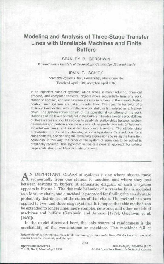
between stations in buffers. A schematic diagram of such a systemappears in Figure 1. The dynamic behavior of a transfer line is modeledas a Markov chain, and a method is proposed for finding the steady stateprobability distribution of the states of that chain. The method has beenapplied to two- and three-stage systems. It is hoped that this method canbe extended to longer lines, more complex networks, and other models ofmachines and buffers (Gershwin and Ammar [1979]; Gershwin et al.[1980]).
In the model discussed here, the only source of randomness is theunreliability of the workstations or machines. The machines fail at
Subject clamfication: 343 inventory levels and throughput in transfer tines. 570 Markov chain model oftransfer lines, 721 reliability and storage.
354OperatJons Research 0030-364X/83/3102-0354 $01.25Vot. 31, No. 2. March-April 1983 © 1983 Operations Research Society of America
Buffered Transfer Lines 355
tt)
<
S " Z
356 Gershwin and Schick
random times and remain inoperable for random periods while they areunder repair. It is possible to compensate for workstation failures byproviding redundancy, i.e., secondary parallel stations that are broughtinto use in case of failures of primary machines. This process, however,can be prohibitively expensive if system components are costly.
An alternative is to place buffer storages between unreliable stages.These provide temporary storage space for the products of stationsupstream of a failed station. Similarly, they provide temporary supphesof workpieces for stations downstream of a failed station. Thus, theydecrease the effects of workstation failures on the rest of the hne.
However, costs of floor space, material handling equipment, and in-process inventory are also important. It is thus necessary to find the"best" storage configuration; this leads to an optimization problem. Tosolve this problem, it is essential to quantify the relations betweentransfer line design parameters (i.e. average up and down times ofworkstations, storage capacities) and the performance measures.
According to Buzacott [1967a], transfer lines were first studied analyt-ically via a probabilistic approach by Vladzievskii [1952]. Applications ofqueueing networks and transfer line models are found in a wide range ofareas, including computer science; coal mining; the cotton, paper andchemical industries; aircraft engine overhauling; and the automotive andmetal cutting industries.
The production rate of transfer lines in the absence of buffers and inthe presence of buffers of infinite capacity has been studied by manyresearchers, including Hunt [1956], Suzuki [1964], Avi-Itzhak and Yadin[1965], Morse [1965], Buzacott [1967a, 1968], Barlow and Proschan[1975], and Rao [1975a]. Some authors analyze rehable transfer lineswhere buffers are nsed to reduce the effects of fluctuations in nondeter-ministic service times (Patterson [1964], Hillier and Boling [1966],Neuts[1968, 1970], Hatcher [1969], Knott [1970a, b], Muth [1973], Ammar andGershwin [1980a]).
Unreliable two-stage systems with finite buffers have been studied(Sevast'yanov [1962], Buzacott [1967a, b; 1969; 1972], Gershwin [1973],Rao [1975a, b], Artamonov [1976], Okamura and Yamashina [1977],Schick and Gershwin [1978], Berman [1979], Gershwin and Berman[1981]). Longer systems are more difficult to analyze because of thecomplexity of machine interference when buffers are full or empty (Oka-mura and Yamashina [1977]). Such systems have been formulated inmany ways (Hildebrand [1968], Hatcher [1969], Knott [1970a, b], Sheskin[1974, 1976], Gershwin and Schick [1977], Buzacott and Hanifin [1978]);and studied by approximation (Sevast'yanov, Buzacott [1967a, b], Masso[1973], Masso and Smith [1974]); as well as simulation (Barten [1962],Freeman [1964], Anderson [1968], Anderson and Moodie [1969], Kay[1972], Hanifin et al. [1975a, b]. Ho et al. [1979]).
Buffered Transfer Lines 357
Some analysts have computed the ergodic probability distribution bysolving the systems of transition equations, either by straightforwardinversion (e.g., Okamura and Yamashina, for two-stage lines) or byexploiting the structure of the system of equations (Schick and Gershwin,Gershwin and Schick [1979a] use its block-tridiagonal structure). Bothapproaches are severely limited by memory and numerical precision.
The only analytic techniques for lines with more than two unreliablestages and finite buffers are for very special systems (Sheskin [1974,1976], Soyster and Toof [1976], Soyster et al. [1979]). In these systemsthe probability that a machine is under repair during a given cycle isindependent of the state of that machine during the previous cycle. Thisrestrictive assumption is not needed in this paper.
This paper is a summary of the two- and three-machine transfer lineresults reported in Schick and Gershwin, and Gershwin and Schick[1979b; 1980a].
1. OVERVIEW OF THE METHOD
To find the steady-state probability distribution of an M-state Markovchain, it is necessary to solve a set of M linear transition equations in Munknowns. In the problem discussed here, M is large, so an efficientmethod is required.
This problem does have a structure that can be exploited. It is possibleto find / vectors ^1, • • • , ^,, each of which satisfies at least M - I of thetransition equations. The number of equations which are unsatisfied forat least one vector is /. Consequently if the probability vector is expressedas a linear combination of these vectors.
P = lUCjij (1.1)
then it is guaranteed to satisfy the M — I equations each > satisfies. Inorder to satisfy the remaining equations, the coefficients C, must beappropriately chosen.
This requires solving / linear equations in I unknowns. Since / is muchsmaller than M, it is relatively easy to do. For example, in the two-machine transfer line M = 4(iV + 1) where N is the capacity of the bufferand / = 2.
In the three-machine line M = 8(Ni + 1)(A 2 + 1) (where N, is thecapacity of buffer i) and / = 4(A i + N2) - 10. Clearly, when Ni and A2are large, / is much smaller than M. However, the / equations in the /unknowns Ci, • • • , C/ are poorly behaved for large /. It has been necessaryto use extended precision (32 decimal place) arithmetic to obtain 5decimal place precision in analyzing transfer lines with large storages.Even though / increases more slowly than M, it still limits the size of theproblem that can be treated. This increase prevents the method, ascurrently formulated, from being usefully applied to longer lines.

358 Gershwin and Schick
The approach presented here can be seen as a general technique forsolving large scale structured Markov chain problems. It should beconsidered a philosophy however, rather than a mechanical tool. Applyingthis technique to specific problems necessitates a great deal of analyticalwork. The benefit of the method is that it uses the structure of the chainto substantially reduce the size of the linear system to be solved. At thesame time, there is a loss of sparsity and, as a result, the problem maybecome ill-conditioned.
Herzog et al. [1975], and Morrison [1980] suggest methods which arealso based on Equation 1.1 but which use basis vectors ^j which areconstructed in very different ways. Both methods use the problem struc-ture to effectively reduce the dimensionality of the system of linearequations that must be solved. Herzog et al. describe their method as ageneral technique. However, the examples they describe have boundarieswhich are much simpler than those of the present problem. Morrisonmakes no claims for generality, and it appears that his technique dependscrucially on certain features of the internal equations.
2. THE UNRELIABLE TRANSFER LINE WITH INTERSTAGE BUFFERSTORAGES
The system under study consists of a linear network of servicingstations (machines) separated by finite capacity buffer storages (Figure1). Workpieces enter the first machine from outside the system. Eachworkpiece is processed by machine 1, after which it moves to storage 1.The part moves in the downstream direction, from machine i to storagei and on to machine i + 1, until it is processed by the last station, machinek, and leaves the system.
The specific nature of the machine operations is of no consequence inthe present analysis. It is assumed, however, that there is a common,fixed, cycle time and all machines that are operating on pieces start atthe same instant.
The buffer is a storage element. Parts pass through a buffer with atratisportation delay that is negligible compared to service times in themachines, except for the delay caused by other parts in the queue.
Machines fail occasionally. Failures may have many causes and thus,the down-times of failed machines, like the up-times of operating ma-chines, are random variables. When a failure occurs, the level in theadjacent upstream storage may rise. If the failure persists long enough,that storage fills up and forces the machine upstream of it to stopprocessing parts. Such a forced down machine is blocked. Similarly, thelevel of the adjacent downstream storage may fall during a failure, as thedownstream machines drain its contents. If the failure persists longenough, the adjacent downstream storage empties and the machine
Buffered Transfer Lines 359
downstream of it stops processing parts. Such a forced down machine isstarved. These effects propagate up and down the line if the repair is notmade promptly.
By supplying both workpieces and room for workpieces, interstagebuffer storages partially decouple adjacent machines. While machinefailures are to some extent inevitable, the effects of a failure of one of themachines on the operation of others is mitigated by the buffer storages.When storages are empty or full, however, this decoupling effect cannottake place. Thus, as the capacities of storages increases, the probabilityof storages heing empty or full decreases and the effects of failures on theproduction rate of the system are reduced. However, an inevitable con-sequence of buffers is in-process inventory. As buffer capacities increase,more partially completed material is present between processing stages.
For each machine in a A-stage transfer line, its operating condition atis defined by
{0 if machine i is under repair, . , ,
1 if machine i is operational,Here, operational means that the machine is capable of processing a
workpiece. Processing actually takes place only if there is at least onepart in the buffer upstream, and at least one empty slot in the bufferdownstream. (Certain authors, e.g., Kraemer and Love [1970], Okamuraand Yamashina, define two additional machine states, for times when amachine is starved or blocked. This is avoided in the present formulation.)
For each storage J, the variable n^ is defined to be the number ofworkpieces in the storage. Each storage has a maximum capacity Nj, i.e.,0 < Wy < A(/,7 = 1, • • • ,k — 1. The state of the system at time t is definedas
sit) = inAt), ••• , nk-iit), a,it), • • • , aM)) (2.1)
where /, an integer, denotes time in machine cycles.The number of all possible system states is given hy M = 2*(iV] +
1) • • • iN/,-i + 1). In order to calculate such quantities as the averageproduction rate, the average quantity of in-process inventory, and thefraction of time each storage is full or empty, the probability of each ofthe M states of Equation 2.1 must be calculated.
Most assumptions made here in formulating the mathematical modelare standard. (See Koenigsberg [1959] and Buzacott and Hanifin.)
(i) An inexhaustible supply of workpieces is available upstream of thefirst machine in the line, and an unlimited storage area is presentdownstream of the last machine. Thus, the first machine is never starved,and the last machine is never blocked.
(ii) All machines have equal and constant service times. (This assump-tion should be compared with those of Buzacott [1972], Gershwin and
360 Gershwin and Schick
Berman, and Berman). Time is scaled so that this machine cycle takesone time unit. Transportation takes negligible time compared to machin-ing times. AH operating machines start their operations at the sameinstant.
(iii) Machines are assumed to have geometrically distributed timesbetween failures and times to repair. If machine i begins processing aworkpiece, there is a constant probability p, that it fails during that cycle.Thus, the mean operating time (in cycles) between failures is 1/p,.Similarly, if machine i is failed at the beginning of a cycle, there is aconstant probability r, that it is repaired during that cycle. Thus, themean time (in cycles) to repair is 1/r,.
(iv) Machines fail only while processing workpieces. Thus, if machinei is operational (a, = 1) but starved (n,-i = 0) or blocked (n. = Ni), itcannot fail.
(v) Workpieces are not destroyed or rejected at any stage in the line.Partly processed workpieces are not added into the line. When a machinebreaks down, the workpiece it was operating on is returned to theupstream storage to wait for the machine to be repaired so that processingcan resume.
(vi) The convention adopted is that a cycle begins with a transition inthe machine operating conditions and ends with a transition in storagelevel. The latter is determined by the new machine states.
The probabilistic model of the system is studied in steady state. Thus,all effects of start-up transients have vanished and the system behaviormay be represented by a stationary probabihty distribution.
By Assumption iii a machine that is processing a part has a probabilityof failure pi. When the machine is operational but forced down (eitherstarved or blocked), it cannot fail. The probability that an operatingmachine remains operational is 1 — p,. The probability that a failedmachine is repaired by the end of any cycle is r,, independent of storagelevels. A failed machine remains down at the end of a cycle withprobability 1 — r,.
Once machine transitions take place, the new storage level is deter-mined (Assumption vi). This value is dependent on the new states of theadjacent machines. If the upstream machine is processing a part, the partis added to the storage; if the downstream machine is processing a part,it is removed from the storage. The new storage level also depends on thestorage levels immediately upstream and downstream at the end of theprevious cycle. For example, if machine i is operational ia,{t -t- 1) = 1)and the upstream storage was not empty (n,-i(O > 0), a new piece entersstorage i.
The two-machine version of this model differs from Buzacott [1967a]in two important ways. First, Assumption vi reverses the convention on
Buffered Transfer Lines 361
the order of events during a processing cycle. Second, Buzacott ignoresevents of small probability, such as the simultaneous failure and repair oftwo machines. With the method described here, it is more convenient notto ignore these events.
The failure and repair probabilities are used in obtaining the statetransition probabilities, defined by Tii,j) = prob[s(f -I- 1) = i\sit) = j].This matrix is related to the probabilities of machine repair and failureand of buffer level changes by prob[s(( -I- l)|s(()] = (n^=i' proh[niit +l)|n,-i(O, aiit + 1), mil), a,^iU + D, m+iit)) (jl?.! prob[a,(( + l)\ni-i(t),aiit), n,it)]) where for convenience, n^i{t) > 0, nk(t) < N* = oo, so that theconditions noit) > 0 and nkit) < N/, are always satisfied.
Note that for all i,j, T{iJ) > 0,
£.T(i ,» = l, (2.2)
and the resulting Markov chain is ergodic (Gershwin and Schick[1979b]). That is, there is a unique probability distribution satisfying
l (2.3)and i:,p(O = l. (2.4)
The steady-state probabilities [pii)] are used in computing importantperformance measures, namely efficiency (production rate), in-processinventory ni = Eint), and forced down (starvation and blockage) proba-bilities (prob[n,-] = 0] and prob[n., = N,]).
The efficiency Ek of a transfer line is the probability that a pieceemerges from the line during any given cycle. Since the machine cyclesare fixed and equal, efficiency is equal to the production rate per machinecycle. It is given by (Schick and Gershwin), Eh = prob[aA = 1, n*-i > 0].
The behavior of these measures as a function of the system parametersipi and r,, i = 1, 2, 3, and Ni, ( = 1, 2) is illustrated in Schick andGershwin, Pomerance [1979], and Gershwin et al. See also Section 5.
3. ANALYTIC SOLUTION OF INTERNAL TRANSITION EOUATIONS
Equations 2.3 and 2.4 comprise a large system, whose dimensionincreases with the product of the buffer capacities. The technique pre-sented here for efficiently solving this system necessitates that the statesbe separated into two basic classes: internal and boundary.
Internal states are those in which
2 < ni < iV, - 2 for all i = 1, •-- , k - 1. (3.1)
It is important to notice that for any ni to satisfy (3.1), it is necessarythat M > 4 for all i. (The method described here can be extended tocases where Ni is less than 4. Such cases differ in detail, but not inconcept, from those treated here.)
362 Gershwin and Schick
Internal transition equations are those that involve only internalstates. They are the equations in which the final state i as well as all theinitial statesy from which there is a nonzero transition probability in (2.3)are internal.
When a state is internal, all the operational machines can transferparts from their upstream to their downstream storages. In other words,no machine is starved or blocked. Then, the final level of storage i isgiven in terms of its initial level and the final operating conditions ofadjacent machines by
niit + 1) = mit) + adt + 1) - a,Mt + 1). (3.2a)
This is in keeping with the convention (Assumption vi) that in each cycle,machine states change before storage levels.
In the sequel, the following notation will be used for clarity: s' = (/i/,• • • , n'k-u ai, . • • , ak') = sit), and s = (m, - • . , «*_,, ai, - • • , a*) =sit + 1). Thus, (3.2a) may be rewritten as
n, = n/ + ai- ai+i. (3.2b)
For internal state transitions, the machine transition probabilities mayall be combined in a single expression as
|n;-,, a.', «/] = [(1 - ri)'^-'rr-y-'-[a -prp}-"'p'.
If s and s' satisfy (3.2), the transition probability is thus
T(s, s') = n?-i [(1 - rO^-VfO'-^'td -p.)"??.-""']"''-
The set Sis) is defined to be the set of all states s' such that given Wi,• • • , /lA-i and ai, - • • , a*, the initial storage levels n/, • • • , nk-i satisfyEquation 3.2. Equation 2.3 becomes
pis) = Z-^sisi T{s, s')pis') ,
where s and s' are related by (3.2).It is assumed here that the steady-state probability distribution for
internal states has a sum-of-products form:
pis) = S - i Cj^is, Xij, . . . . X*-,j, Yi^ - - . , Ykj) (3.4)
where • • i
^(s, Xij, • • • , Xk-i,j, Yij, • • • , Ykj)
= X'^)... X^kttjYt) . . . y^5 (3.5)
and CJ, Xij, and Yy are parameters to be determined. These parametersmust be such that the internal transition equations (3.3) are satisfied.This is an extension of the product form solution (Baskett et al. [1975]).
Buffered Transfer Lines 363
The number of terms in the summation. A, is crucial to the numericalbehavior of this method. The value of A is calculated for two- and three-machine cases in Section 4.2.
To satisfy (3.3), these equations are treated as if they were an ordinarydifferential equation boundary-value problem. In a differential equationof order n, there may be n distinct solutions. Although each of thesesolutions by itself satisfies the equation, only a certain linear combinationof these solutions satisfies the boundary equations. Thus, although thetrue probabilities are given by summations of the form of Equation 3.4,Xij are chosen so that each element in the sum by itself satisfies theinternal transition equations.
If a single term in the summation (3.4) is substituted into (3.3), thefollowing is obtained:
.[(1 -pi)''-p}-''-
where the subscript J is suppressed for clarity. Using Equation 3.2 andsimplifying,
= L. ." • • S"*- IT'-i [(1 - ry-^rr-V-'-^Xil - pd''-p}-"-Yif'.
Note that n, and n/ no longer appear. Dividing both sides byn t i ( l -r ,) ' -" ' rf-leads to
nf-i (Z?'-"-Y?')/((l - ry-^Tf) gg
where for convenience, Xk is defined to be 1. Note that a,' only occurs asan exponent in the right hand side of Equation 3.6; furthermore, a,' onlytakes the values 0 and 1. The following lemma is used to simplifyEquation 3.6:
LEMMA 3.1. For any numbers Ai, • • • , Ak, 2i-o *" *
Proof. Proceeding by induction, it is easy to see that the equation issatisfied for k = 1. Assuming that the equality holds for k, the left side is,for k + 1,
Z l v l V ' TT*+1 A <fi
t n*-i' (1+A.).

364 Gershwin and Schick
Using Lemma 3.1, the right hand side of (3.6) is rewritten asn*-i [1 +
When this is substituted into (3.6), the variables a,' (but not a,) vanish.Simplifying leads to
nt i Jtr'-'-y?' = n*-i [u - ry-'-rr- + d - PJ-'PZ-'Y,]. (3.7)
Equation 3.7 has been derived with no condition on a,; thus, it must holdfor all values of a,. In particular, if a, = 0 for i = 1, • • - , k, then (3.7)reduces to:
l = n * - i [ l - r , + p.Yi]. (3.8)
If ah = 1, and a. = 0 for i = 1, ... ,k,i¥= h, then (3.7) becomes
Xhl^X^Yf, = n?.i.i^/, [l-n + PiYi]-[r, + (1 - pft) Y/,] (3.9)
where, again for convenience, Xo is defined to be 1. Using (3.8), Equation3.9 can be reduced to
= (r, + (1 - A ) Y,)/(l - r, + p,Yi), i = I, •.. , k. (3.10)
Any other sets of values for a, in Equation 3.7 give equations that mayreadily be derived from (3.8) and (3.10). Equations 3.8 and 3.10 arereferred to as parametric equations in the sequel.
Since XQ = Xk = 1, there are k + 1 equations in 2A — 1 unknowns.Furthermore, the weighting and normalizing constants Cj remain to becomputed. In the following sections, the analysis of two- and three-machine lines is completed. This requires the analysis of the parametricequations for A = 2 and 3.
The following notation will be used: U = (Xi, • • • , Xk-i, Yj, . • • , Y*),f > = iX]j, • - • , Xk-ij, Yij, • • • , Ykj).
When k = 2, (3.8) and (3.10) are three equations in three unknowns.They can be combined into a single quadratic equation in one unknown.The solutions are
Y , i - r , / p , ; ( = 1 , 2 , J , * " ^*
Ai2 = Y22/Y12 "
Yi2 = (n + r2- rir2 - p2ri)/{p\ + pt- pip2 - p^rz) I - (3.12)
Y22 = (n + r2- nrz - pir2)/ipi + pi- P1P2 - pan) J
4. THE THREE-MACHINE CASE
The first task is the calculation of expression ^(x, U) for every state s.For internal states, this is done in Section 3. Transient states, states ofinternal form, and states of other forms are considered in Section 4.1.
Buffered Transfer Lines 365
Expressions are found for all states s, but these expressions do notsatisfy all the transition equations. A small subset of the boundary statesQ, remains in which the error gis, U) = |(s, U) — Y.aas' Tis, s')|(s', U) isnot identically zero, i.e., not zero for all U. These errors are used tochoose the constants C, in (3.4) so that all the transition equations aresatisfied. It is important to note that the set of expressions |(s, U) derivedin this section is not unique. It is hoped that this set results in a relativelycompact solution, i.e., that S2 contains few states.
There are two kinds of boundary states in a three-stage line; edgestates and corner states. Edge states are those in which one storage levelis internal and the other is not. Corner states are those in which neitherstorage is internal.
4.1. Transient States, States of Internal Form, and Other Forms
Since transient boundary states have zero steady-state probability, thechoice ^(s, U) = 0 suggests itself Finding expressions for the transientstates is clearly not hard. Finding the transient states themselves is. Thefull set of transient states can be established by the following rules.
(i) States where a, = 0 and either n,-i = 0 or /i, = Ni are transient. Thisis because a starved or blocked machine cannot fail.
(ii) States where machine i — 1 is operating (i.e., not starved orblocked), ni-i = 1, and a, = 0; or a, = 0, n, = N, — 1 and machine i + 1 isoperating, are transient. This is because machine i could not have failedif «,-] = 0 orn, = iV,, and an operating machine upstream or downstreamwould have incremented the storage by plus or minus one, respectively,in the cycle during which machine i failed.
(iii) States where machine i — 1 is operating and n.,-i = 0; or n,-i =N,~i and machine i is operating are transient. This is because an operatingmachine upstream or downstream would increment the storage by plusor minus one, respectively, since by Assumption vi of Section 2, machinetransitions precede and determine storage transitions.
(iv) It is important to note the following exceptions: (1, 0, 1, 1, 1) canbe reached from (0, 0, 0, 1, 1), (1, 1, 1, 1, 0) can be reached from (0, 1, 0,1, 1), (Ni, Na - 1 , 1, 1, 1) can be reached from (Nj, Na, 1, 1, 0), and(Ni -1,N2- 1, 0, 1, 1) can be reached from (M - 1, N2, 1, 1, 0). Thesestates are not transient.
The fact that machine 1 is never starved and machine 3 (for k = 3) isnever blocked must be considered in deriving the transient states.
It is easy to derive | expressions for certain states. For example, thetransition equation for p(l, 2, 0, 1, 1) involves only states of the form (2,2, ai, a-iy a:)), all of which are internal. If (3.5) and the parametric equationsare used, a natural choice for ^(1, 2, 0, 1, 1, U) is the internal form ^(1, 2,0, 1, 1, U) = XiX-i'YzYa. Similarly, it can be shown that ^(1, na, 0, 1,1, U) = XiX^'Y-zYs for aU 2 < na < N2 - 2.
366 ' Gershwin and Schick
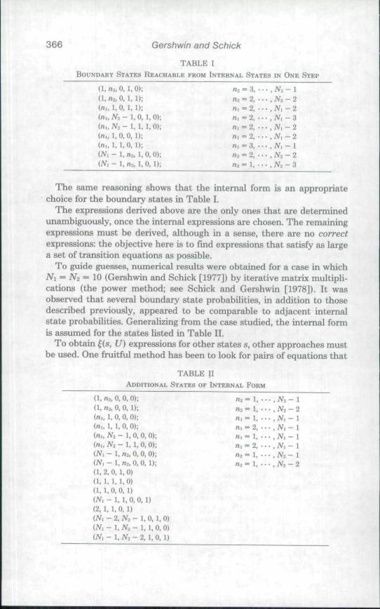
TABLE IBOUNDARY STATES REACHABLE FROM INTERNAL STATES IN ONE STEP
(l,na, 0,1,0); na = 3, ••• , iV2- 1
( 1 , nz, 0, 1,1); /la = 2, . . . . Na - 2(n,. 1,0,1, 1); n, = 2, • . . .N , - 2(n,, M - 1, 0,1, 0); n, = 2, . . . , N, - 3(n,, Ni - 1, 1,1, 0); n, = 2, - . . , N, - 2(ni, 1, 0, 0, 1); Oi = 2. • • • , N, - 2(n,, 1, 1,0, 1); n, = 3, ••• ,N , - 1(N, - 1, na, 1, 0, 0); na = 2, • • • , Na - 2(N, - 1, na, 1, 0, 1); na = 1. . • • , Na - 3
The same reasoning shows that the internal form is an appropriatechoice for the boundary states in Table I.
The expressions derived above are the only ones that are determinedunambiguously, once the internal expressions are chosen. The remainingexpressions must be derived, although in a sense, there are no correctexpressions: the objective here is to find expressions that satisfy as largea set of transition equations as possible.
To guide guesses, numerical results were obtained for a case in whichNi = N2= 10 (Gershwin and Schick [1977]) by iterative matrix multipli-cations (the power method; see Schick and Gershwin [1978]). It wasobserved that several boundary state probabilities, in addition to thosedescribed previously, appeared to be comparable to adjacent internalstate probabilities. Generalizing from the case studied, the internal formis assumed for the states listed in Table II.
To obtain ^(s, U) expressions for other states s, other approaches mustbe used. One fruitful method has been to look for pairs of equations that
TABLE IIADDITIONAL STATES OF INTERNAL FORM
(1,(1,(n.(n,in,(n,(N(N
(1.<1.(1,(N,(2.(N,(Ni
(N,
n-i, 0, 0, 0);"2, 0. 0, I);, 1, 0, 0, 0);. 1. 1. 0, 0);, Na - 1, 0. 0, 0);. Na - 1, 1, 0, 0);, - 1, na, 0, 0, 0);, - 1, na, 0, 0, 1);2, 0, 1, 0)1, 1, I, 0)1, 0, 0, 1)1 - 1, 1,0,0, 1)1.1,0,1)1 - 2, Na - 1, 0, 1, 0)I - 1, Na - 1, 1. 0, 0)1 - 1, No - 2, I, 0, 1)
na =112 =
ni =
rti =
n, =n, -'n2 =na =
1. ••• .1 . • • • ,
1 . • • • ,
2 , • • • ,
1, . . . .
2. • • • ,1 , • - • ,
1 . • • • .
Na- 1Na-2Ni - 1N, - 1N, - 1N, - 1Na- INa-2
Buffered Transfer Lines 367
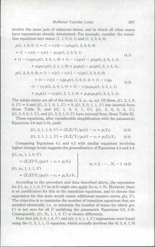
involve the same pair of unknown states, and in which all other stateshave expressions already determined. For example, consider the transi-tion equations into states (1, 1, 0, 0, 1) and (1, 2, 0, 0, 0).
p(l, 1, 0, 0, 1) = (1 - n)(l - r2)r3pih % 0, 0, 0)
+ (1 - r,)(l - r-Ml - p,)pil, 2, 0, 0, 1)(4.1)
+ (1 - rOparapd, 2, 0, 1, 0) + (1 - rOpad - P3)p(l, 2, 0, 1, 1)
, 2, 1. 1, 0) + pip2(l - P3)pil, 2, 1, 1, 1).
p(l, 2, 0, 0, 0) = (1 - r,)(l - r-Ml - r3)p(l, 2, 0, 0, 0)
+ (1 - r,)(l - r2)p3p(l. 2, 0, 0, 1) + (1 - r,)p^ ^^ ^^
•(1 - ra) pil, 2, 0, 1, 0) -t- (1 - ri)p2p3p(l, 2, 0, 1, 1)
+ pipad - r3)p(l, 2, 1, 1, 0) + pip2p3p(l, 2, 1, 1, 1).
The initial states are all of the form (1, 2, ai, a2, 03). Of these, g(l, 2, 1, 0,0, f/) = 0 and ^(1, 2, 1, 0, 1, U) = 0, ^(1, 2, 0, 1, 1, U) has internal form(from Table I), and ^(l, 1, 0, 0, 1, U), ^(1, 2, 0, 0, 0, U),m, 2, 0, 0, 1, U), and ^(1, 2, 0, 1, 0, U) have internal form (from Table II).
These equations, after considerable simplification with the parametricEquations 3.8 and 3.10, yield:
^(1, 2, 1, 1, 0, U) = iX,X2'Y,/p2)il -r2 + P2Y2) (4.3)
^(1, 2, 1, 1, 1, U) = iX,X2'Yi/p2){l - rs + P2Y2)Y3. (4.4)
Comparing Equations 4.1 and 4.2 with similar equations involvinghigher storage levels suggests the generalization of Equations 4.3 and 4.4:
n2, 1,1,0, U)
= (XiXS^y,/p
m, 1,1,1, U)n2 = 2 , . . . , N 2 - l ( 4 . 5 )
According to the procedure and data described above, the expressionfor (1,712, 1, 1, 0, U) in (4.5) might also apply for ng = A2- However, thereis no justification for this in the transition equations, and to choose thisexpression for this state would create additional nonzero errors ^(.s, U).The objective is to maximize the number of transition equations that aresatisfied identically, i.e., to minimize the number of states for which gis,U) is not zero for all U satisfying the parametric Equations 3.8, 3.10.Consequently, ^(1, N2, 1, 1, 0, U) is chosen differently.
Note that ^(0, 2,0, 1, 0, U) and |(0, 2, 0, 1, 1, U) expressions were foundusing the (1, 2, 1, 1, 1) equation, which actually involves the (0, 3, 0, 1, 0)

368 Gershwin and Schick
and (0, 3, 0, 1, 1) states. It was assumed that £(0, 3, 0, 1, 0, U) =^2^(0, 2, 0, 1, 0, U) and |(0, 3, 0. 1, 1, U) = ^2^(0, 2, 0, 1, 1, U). Thecomplete list of expressions is found in Gershwin and Schick [1980a].
For comparison purposes, the complete solution to the two-machineline appears in Table III Note that its boundary structure is a simplifi-cation of the three-machine boundary, with transient states, states ofinternal form, and others. The complete solution technique appears inGershwin and Schick [1980a].
4.2. Construction of the Probability Vector
A small number of boundary transition equations were used to generateeach expression discussed in Section 4.1. It is possible to show, using the
TABLE inSTEADY-STATE PROBABILITIES OF TWO-MACHINE LINE
p(0, 0, 0) = 0p(0, 0.1) = {CX){n + ra - nr2-pplQ, 1, 0) = 0p(0, 1,1) = 0p(l, 0, 0) = CXp(l, 0, 1) = CXY,p(l, 1, 0) = 0
p(n, a,, a^) = CX"YTYt'; 2 s n < W - 2p(iV - I, 0, 0) = CX"-'p{N- 1,0. I) = 0
p(N~ 1,1, 1)p{N, 0, 0) = 0p(N, 0, 1) = 0piN, 1. 0) = {p(N, 1, 1) = 0
X 4 Xi, Yi, and Y2 are given by Equation 3.12; C satisfies (2.4).
parametric equations, that these expressions satisfy many of the remain-ing transition equations identically, i.e., for all values of U.
A significant number / of boundary equations, however, are not satisfiedidentically. The states that these transition equations lead to are called"odd," and the set of odd states is called S2. The number of states linQis much smaller than M. In this section it is shown that the Markov chainmay be solved by solving a set of / linear equations, rather than M. It isalso shown that the number of terms A in (3.4) is equal to /.
For the Markov chain described in Section 2,
Q (4.6)
where / denotes the identity matrix. For a general )fe-stage transfer line,the boundary state probabilities are expressed as a sum of terms, in the

Buffered Transfer Lines 369
form of (3.4). For boundary states s, the |(.s, U) expressions are thosederived at the beginning of Section 4 (for a three-stage transfer line).Note that (3.4) also applies to internal states when ^(s, U) is given by(3.5). Equation 3.4 may he rewritten as
p = :^C (4.7)
where C = [C., • • • , C,f, E = [|(t/,). • - • ,i(t/x)] andm) is a vectorwhose components are ^(s, Uj) for all s. Note that tA, • • • , Ux are Adistinct solutions of the parametric equations. (For A ^ 3, the number ofunknowns exceeds that of equations.) Substituting (4.7) into (4.6),
( r - / ) i C = O. (4.8)
System (4.8) has a nonzero solution C if the matrix (T — / ) i has rankless than or equal to A — 1. Equation (2.4) provides an additional conditionon C which requires that it be nonzero. A unique solution is determinedif the rank of (T — I)B is exactly equal to A — 1.
In Lemma 4.1, it is shown that, for A > /, the rank of a is no greaterthan /. From numerical experience, it appears that for A > Z, if the Uj areall distinct, the rank of i is exactly /. Under this assumption. Lemma 4.2shows that the rank of G is / — 1. In the sequel, we choose A = /.
LEMMA 4.1. //"A > /, the rank of A is at most I.
Proof Let iT - I)j be the yth row of T - /. Matrix H has beencoastructed so that exactly M — loi the M rows ofT- I satisfy (T — /)>i= Q'\ Form the matrix T' by deleting one of the other rows of T— I andreplacing it by p^ = (1, 1, • • • , 1). Again exactly M - I rows T/ of T'satisfy
T/H = ^ . (4.9)
Thii is because v^'Z ^ ^ , which is possible to verify, tediously, using theinternal expressions (3.5), the boundary expressions in Gershwin andSchxk [1980a] and the parametric Equations 3.8 and 3.10. (It is easier todo what the authors did: to verify this numerically.)
Because T is the transition matrix of a Markov chain with a singleergodic final class, T — I has rank M — 1. Equation 2.2 imphes that anyrow of T — / is a linear combination of the others. Furthermore, v^ islinearly independent of all the rows of T — 7. Consequently T' has rankM. Therefore the M — I row vectors in (4.9) are linearly independent.The columns of Z are orthogonal to these vectors. They therefore lie ina subspace of dimension < /, and the lemma is proved.
LEMMA 4.2. Assume \ = I and the rank ofE is I. Then the rank of G is/ — 1 and a unique nonzero C vector exists. (Note: The requirement thatthe rank of i is / is important and limits the set of |(s, V) expressionsthat can be used.)

370 ' Gershwin and Schick
Proof. The rank of T'S is / (Hadley [1964]). Therefore, the rank of(T - I)Z is I or I- 1, since it is the same as T'Z except for one row.
If e is a nonzero vector of dimension M, there is a unique nonzerosolution C to T'ZC = e, provided that component ei is zero for all i suchthat the ith row of T'H is zero. Let e^ be (0, • • - , 0, 1, 0, • • • , 0), wherethe nonzero element is in the location corresponding to the p^ row in T'.Then Q satisfies (4.8) since the row that is replaced in T - / by i- islinearly dependent on the other rows.
If the rank of (T - / ) A were I, the only solution to (4.8) would beQ = 0. Therefore, the rank of (T - / ) i is / - 1. Since G is composed ofthe nonzero rows of (T - I)Z, G also has rank / - 1, and the lemma isproved.
TABLE IVfl. THE SET OF ODD STATES
Comer States
Edge States
(1. 1, 1, 1, I)(M - 1. M - 1,1.1.1)(1, Ni ~ 1,1, 1.1){N, - 1, N-i, 1. 1, 0)(0, 1, 0, 1, 1){Nt. 0, 1, 0, 1)
(n,, 0, 0. 0, 1)(ni, 0,1, 0,1);(0. n-i, 0, 1, 0);
(Ni,na, 1,0,0);iN,, 712. 1, 0, 1);
(ni, N2, 0, 1, 0);(m, N2, 1, 1. 0);
(A?>-( i V , -(0, Naid.Ni
(Nu I,(A^i, 1,(1 . N2,
(1 . N2,
2<ni2<rei2<na
2Znl2sni
2<rt|
2<n.
1,1,-—1.1.0.1,
s<
—
0, 0. 0, 1)0, 1, 0, 1)1. 0, 1, 0)1,0. 1. 1)0,0)0.1)1,0)1.0)
NI - 2N,-2N2-2
N-2~2N-i-2Ni-2N , - 2
Consequently, C is determined by the / linear equations in I unknowns
O . . . , . , (4.10)
and Equation 2.4.The set of odd states, fl, is displayed in Table IV, subdivided into edge
states and corner states. The number of odd edge states depends on thestorage sizes; the number of odd comer states is constant. The totalnumber of odd states, which may be obtained from Table IV by inspec-tion, is / = 4(iVi + N2) — 10. This is linear in storage sizes, while M, thetotal number of system states, is quadratic in storage sizes. Thus, thereduced-order system of Equations 4.10 increases in dimension moreslowly than the original system, (2.3)-(2.4).
(There is exactly one odd edge state in the two-machine case; it hasthe effect of eliminating (3.11) from the sum (3.4).)
Buffered Transfer Lines 371
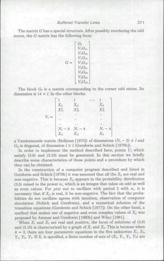
The matrix G has a special structure. After possibly reordering the oddstates, the G matrix has the following form:
Go
G =V2G2
The block Go is a matrix corresponding to the comer odd states. Itsdimension is 14 X /. In the other blocks:
1
Xa
Ni-4 Ni~4
XuXI
Ni-4
a Vandermonde matrix (Bellman [1970]) of dimensions (N, — 3) X / andGij is diagonal, of dimension Ix I (Gershwin and Schick [1979b]).
In order to implement the method described here, points Uj whichsatisfy (3.8) and (3.10) must be generated. In this section we brieflydescribe some characteristics of these points and a procedure by whichthey can be obtained.
In the construction of a computer program described and listed inGershwin and Schick [1979b] it was assumed that all the Xij are real andnon-negative. This is because Xij appears in the probability distribution(3.5) raised to the power m, which is an integer that takes on odd as wellas even values. For pis) not to oscillate with period 2 witb n,, it isnecessary that if X> is real, it be non-negative. The fact that the proba-bilities do not oscillate agrees with intuition, observation of computersimulation (Schick and Gershwin), and a numerical solution of thetransition equations (Gershwin and Schick [1977]). On the other hand, amethod that makes use of negative and even complex values of Xjj wasproposed by Ammar and Gershwin [1980b] and Wiley [1981].
When Xi and X2 are real and positive, the locus of solutions of (3.8)and (3.10) is characterized by a graph of Xi and X2. This is because whenk = ^, there are four parametric equations in the five unknowns Xi, X2,Yi, Y2y Y3. UXi is specified, a finite number of sets of (X2, Vi, Y2, Y3) are

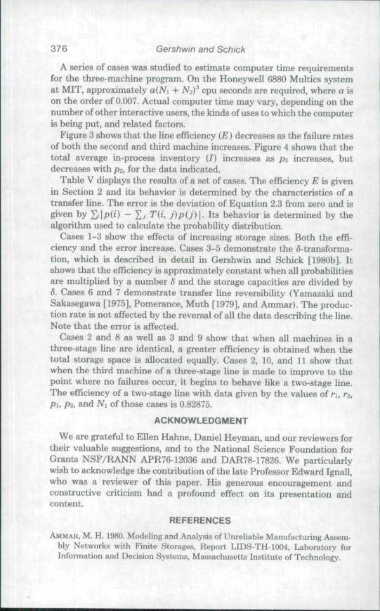
372 Gershwin and Schick
determined. In Figure 2 (Xi, X-2) is plotted. For each (Xi, X2) in this graph,(Yi, Y2, y ) exist such that (3.8), (3.10) are satisfied.
It is shown in Gershwin and Schick [1979b] that either Y,, Y2, Y.i areall positive, or else exactly one of them is negative. All 7, are positive onthe closed curve that passes through (Xi, X-i) = (1, 1) and Y, does notchange the other curves. In addition, the limiting values of Xi and Y, atthe 12 extremes of Figure 2 are calculated.
Figure 2. Locus of (Xy, X2) parameters. For every point on thesecurves, a set of (Yi, Y2, Ya) exists such that (^1, X2, Yi, Y2, Y3) satisfiesEquations 3.8 and 3.10 for k = 3. For this plot, the failure and repairprobabilities are: p, = 0.1, /jj = /J3 = 0.05, n = ra = 0.2, rs = 0.15.
By suitably transforming X, and Y,, it is possible to show that the setof Uj can be generated by repeatedly solving a single quadratic equation.
For A > 3, let Q, = Xi/X.-i, i = i, ... , k. (RecaU that JSCo = Xk = l.) Thisquantity is significant when more general networks are considered(Gershwin and Ammar, and Ammar [1980]). It represents the structureof the network.

Buffered Transfer Lines 373
L e t
Zi = l - n + piY,, i = 1, ••• ,k, (4J1)
W, = Q.Z., i = 1, . . . , A.
Then it can be shown that Wi = (1 - p,)[(Z, - ((1 - r, - p i ) / ( l - p,)))/(Z. - (1 - r.))], i = 1. . . . , A ,
and nf-i ^« = 1- Combining these *
nf-i (1 - pmZi - (1 - n - p,)/(l - Pi))/(Z, - (1 - n))] = 1. (4.13)
If jfe = 3, (4.12) implies that ^2 = (Z1Z3)"'. If this is substituted for Z2 in(4.13), a single equation involving only Zi and Z3 is found. If either Zi orZ3 is assigned a value, this equation reduces to a quadratic equation inthe remaining variable. It can be written in the form (Gershwin andSchick [1980a])
Zs'iAZi" + BZi] + Z-ICZ^ -f- DZi + £ ] + [FZi + G] = 0. (4.14)
In this manner, solving a system of four nonlinear equations is reducedto solving a quadratic equation, since Y", is uniquely determined by Z, andXi by Yi, using Equations 4.11 and 3.10, respectively.
If A > 3, (4.14) becomes an equation in A - 1 variables. If A - 2 arespecified, it is quadratic in the variable remaining.
For A = 3, the procedure is:1. Choose any Zi satisfying 0 < Zi < (1 - r, - Pi)/(1 - Pi) or
Zi > 1 - ri. (This ensures that Wi, Qi, and A", are positive.)2. Solve (4.14) for Z;,.3. For each (Zi, Z3) pair, determine Z2 = (Zi, Z3)~\4. Obtain Yi fi-om (4.11), / = 1, 2, 3.5. Obtain X fi-om (3.10), i = 1, 2, 3.This procedure is repeated / times, so as to generate distinct values
f/i, • • • , Vi. Any set of distinct Ui, • • • , Ui is satisfactory subject to theobservations in Section 5. The matrix G is constructed and Equation 4.10may be solved together with (2.4).
5. NUMERICAL BEHAVIOR
No numerical difficulties have been encountered in implementing thetwo-machine solution. In fact, a version of it has been written for aprogrammable pocket calculator (Ward [1981]). It should be observedthat it is not necessary to calculate the probability of each state if onlythe performance measures of Section 2 are required. By performingseveral summations analytically (including those in the evaluation of C)computational effort and error are reduced.
374 Gershwin and Schick
Some difficulties were found in the three-machine case. First, althoughthe G matrix is considerably smaller than the T matrix, its size growslinearly with storage sizes (4(A i + N-z) - 10). Consequently, computertime and storage requirements grow with Ni and A 2. This method is thusimpractical for large buffers. Furthermore, this approach cannot beextended to larger systems without conceptual modification.
Second, the numerical behavior of the G matrix deteriorates as Ni andN2 grow. Although Lemma 4.2 shows that the nullity of G is 1, this is true
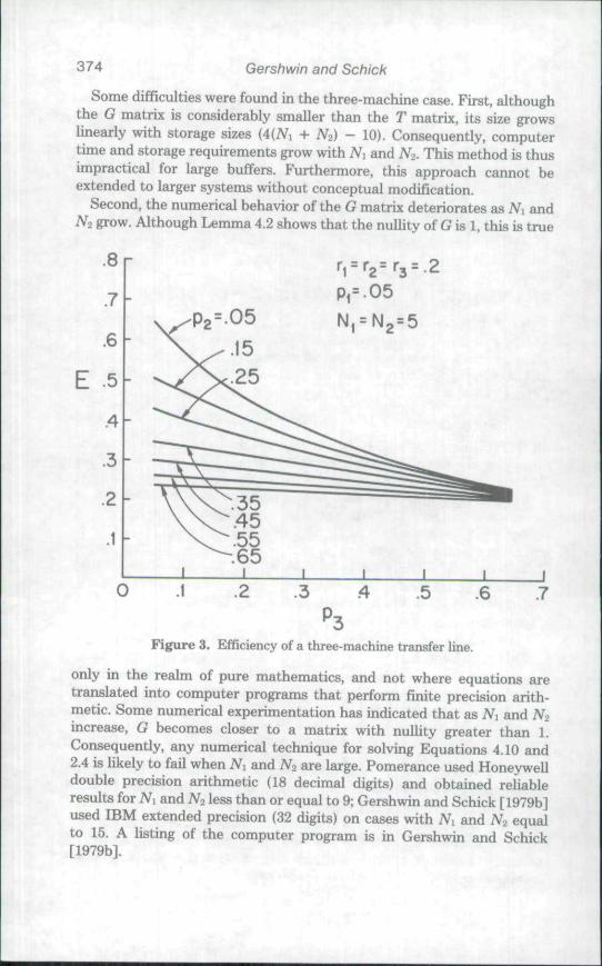
Figure 3. Efficiency of a three-machine transfer line.
only in the realm of pure mathematics, and not where equations aretranslated into computer programs that perform finite precision arith-metic. Some numerical experimentation has indicated that as A i and A'2increase, G becomes closer to a matrix with nullity greater than 1.Consequently, any numerical technique for solving Equations 4.10 and2.4 is likely to fail when Ni and N2 are large. Pomerance used Honeywelldouble precision arithmetic (18 decimal digits) and obtained reliableresults for M and N2 less than or equal to 9; Gershwin and Schick [1979b]used IBM extended precision (32 digits) on cases with Ni and M equalto 15. A listing of the computer program is in Gershwin and Schick[1979b].
Buffered Transfer Lines 375
I
10
9
8
7
6
5
4
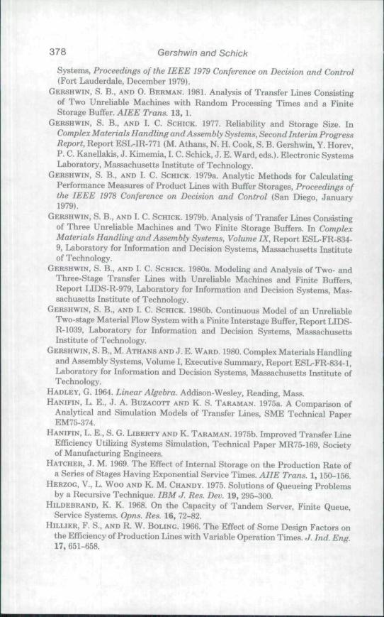
3Pi=05
0 .2 .3 .4 .5 .6 .7
Figure 4, Expected in-process inventory.
Experience suggests that any set of (Z|, Z2, Z3) triplets generatedaccording to the procedure of Section 4 is satisfactory, provided thestorages are not large. That is, when N] and N-z are small, there is noapparent difficulty associated with numerical or analytic singularity ofthe G matrix. However, as M and N2 increase the matrix becomes closeto numerical singularity.
TABLE VA SET OF CASES AND RESULTS
Case
1234567891011
.09
.09
.09
.18
.225
.09
.18
.09
.09
.09
.09
Ta
.09
.09
.09
.18
.225
.225
.225
.09
.09
.09
.09
.09
.09
.09
.18
.225
.18
.09
.0909.09.09
PI
.01
.01
.01
.02
.025
.025
.01
.01
.01
.01
.01
.01
.01
.01
.02
.025
.02
.02
.01
.01
.01
.01
Pa
.01
.01
.01
.02
.025
.01
.025
.01
.01
.001
.0001
A'l
451054484555
N2
4510548461555
E.7676.7743
.8000
.7933
.7895
.7358
.7358
.7741
.7967
.8236
.8282
Error
.7X 10 '*
.6 X 10"''
.7 X 10*
.1 X 10"'
.4 X 10"'
.2 X 10"'"
.1 X 10"'"
.2 X 10"'''
.9 X 10""
.4 X 10 '"
.2 X 10"'"
376 Gershwin and Schick
A series of cases was studied to estimate computer time requirementsfor the three-machine program. On the Honeywell 6880 Multics systemat MIT, approximately a(M + Nz)^ cpu seconds are required, where a ison the order of 0.007. Actual computer time may vary, depending on thenumber of other interactive users, the kinds of uses to which the computeris being put, and related factors.
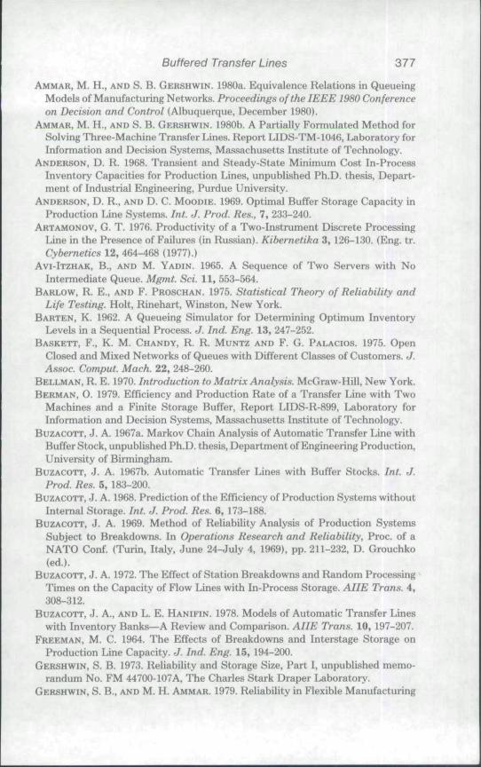
Figure 3 shows that the line efficiency iE) decreases as the failure ratesof both the second and third machine increases. Figure 4 shows that thetotal average in-process inventory (/) increases as ps increases, butdecreases with p2, for the data indicated.
Table V displays the results of a set of cases. The efficiency E is givenin Section 2 and its behavior is determined by the characteristics of atransfer line. The error is the deviation of Equation 2.3 from zero and isgiven by S'|p(O - Sy TH, j)p{J)\. Its behavior is determined by thealgorithm used to calculate the probability distribution.
Cases 1-3 show the effects of increasing storage sizes. Both the effi-ciency and the error increase. Cases 3-5 demonstrate the 5-transforma-tion, which is described in detail in Gershwin and Schick [1980b]. Itshows that the efficiency is approximately constant when all probabilitiesare multiplied by a number S and the storage capacities are divided byS. Cases 6 and 7 demonstrate transfer line reversibility (Yamazaki andSakasegawa [1975], Pomerance, Muth [1979], and Ammar). The produc-tion rate is not affected by the reversal of all the data describing the line.Note that the error is affected.
Cases 2 and 8 as well as 3 and 9 show that when all machines in athree-stage line are identical, a greater efficiency is obtained when thetotal storage space is allocated equally. Cases 2, 10, and 11 show thatwhen the third machine of a three-stage line is made to improve to thepoint where no failures occur, it begins to behave like a two-stage line.The efficiency of a two-stage line with data given by the values of ri, r2,Pu p2, and Ni of those cases is 0.82875.
ACKNOWLEDGMENT
We are grateful to Ellen Hahne, Daniel Heyman, and our reviewers fortheir valuable suggestions, and to the National Science Foundation forGrants NSF/RANN APR76-12036 and DAR78-17826. We particularlywish to acknowledge the contribution of the late Professor Edward Ignall,who was a reviewer of this paper. His generous encouragement andconstructive criticism had a profound effect on its presentation andcontent.
REFERENCES
AMMAR, M. H. 1980. Modeiing and Analysis of Unreliable Manufacturing Assem-bly Networks witb Finite Storages, Report LIDS-TH-1004, Laboratory forInformation and Decision Systems, Massachusetts Institute of Technology.
Buffered Transfer Lines 377
AMMAR, M. H., AND S. B. GERSHWIN. 1980a. Equivalence Relations in QueueingModels of Manufacturing Networks. Proceedings of the IEEE WHO Conferenceon Decision and Control (Albuquerque, December 1980).
AMMAR, M. H., AND S. B. GERSHWIN. 1980b. A Partially Formulated Method forSolving Three-Machine Transfer Lines. Report LIDS-TM-1046, Laboratory forInformation and Decision Systems, Massachusetts Institute of Technology.
ANDERSON, D. R. 1968. Transient and Steady-State Minimum Cost In-ProcessInventory Capacities for Production Lines, unpublished Ph.D. thesis. Depart-ment of Industrial Engineering, Purdue University.
ANDERSON, D. R., AND D. C. MOODIE. 1969. Optimal Buffer Storage Capacity inProduction Line Systems. Int. J. Prod. Res., 7, 233-240.
ARTAMONOV. G. T . 1976. Productivity of a Two-Instrument Discrete ProcessingLine in tbe Presence of Failures (in Russian). Kibernetika 3,126-130. (Eng. tr.Cybernetics 12, 464-468 (1977).)
AVI-ITZHAK, B., AND M. YADIN. 1965. A Sequence of Two Servers with NoIntermediate Queue. Mgmt. Sci. 11, 553-564.
BARLOW, R. E., AND F. PROSCHAN. 1975. Statistical Theory of Reliability andLife Testing. Holt, Rinehart, Winston, New York.
BARTEN, K. 1962. A Queueing Simulator for Determining Optimum InventoryLevels in a Sequential Process. J. Ind. Eng. 13, 247-252.
BASKETT, F., K. M. CHANDY, R. R. MUNTZ AND F. G. PALACIOS. 1975. OpenClosed and Mixed Networks of Queues with Different Classes of Customers. J.Assoc. Comput. Mach. 22, 248-260.
BELLMAN, R. E. 1970. Introduction to Matrix Analysis. McGraw-Hill, New York.BERMAN, 0. 1979. Efficiency and Production Rate of a Transfer Line witb Two
Machines and a Finite Storage Buffer, Report LIDS-R-899, Laboratory forInformation and Decision Systems, Massacbusetts Institute of Tecbnology.
BUZACOTT, J. A. 1967a. Markov Chain Analysis of Automatic Transfer Line withBuffer Stock, unpublished Ph.D. thesis. Department of Engineering Production,University of Birmingham.
BUZACOTT, J. A. 1967b. Automatic Transfer Lines with Buffer Stocks. Int. J.Prod. Res. 5, 183-200.
BUZACOTT, J. A. 1968. Prediction of the Efficiency of Production Systems withoutInternal Storage. Int. J. Prod. Res. 6,173-188.
BUZACOTT, J. A. 1969. Method of Reliability Analysis of Production SystemsSubject to Breakdowns. In Operations Research and Reliability, Proc. of aNATO Conf. (Turin, Italy, June 24-July 4, 1969), pp. 211-232, D. Grouchko(ed.).
BUZACOTT, J. A. 1972. Tbe Effect of Station Breakdowns and Random ProcessingTimes on the Capacity of Flow Lines with In-Process Storage. AIIE Trans. 4,308-312.
BUZACOTT, J. A., AND L. E. HANIFIN. 1978. Models of Automatic Transfer Lineswith Inventory Banks—A Review and Comparison. AIIE Trans. 10, 197-207.
FREEMAN, M. C. 1964. The Effects of Breakdowns and Interstage Storage onProduction Line Capacity. J. Ind. Eng. 15, 194-200.
GERSHWIN, S. B. 1973. Reliability and Storage Size, Part I, unpublished memo-randum No. FM 44700-107A, Tbe Cbarles Stark Draper Laboratory.
GERSHWIN, S. B., AND M. H. AMMAR. 1979. Reliability in Flexible Manufacturing
378 Gershwin and Schick
Systems, Proceedings of the IEEE 1979 Conference on Decision and Control(Fort Lauderdaie. December 1979).
GERSHWIN, S. B., AND O. BERMAN. 1981. Analysis of Transfer Lines Consistingof Two Unreliable Machines with Random Processing Times and a FiniteStorage Buffer. AIEE Trans. 13, I.
GERSHWIN, S. B., AND I. C. SCHICK. 1977. Reliability and Storage Size. InComplex Materials Handling and Assembly Systems, Second Interim ProgressReport, Report ESL-IR-771 (M. Athans, N. H. Cook, S. B. Gershwin, Y. Horev,P. C. Kanellakis, J. Kimemia, I. C. Schick, J. E. Ward, eds.). Electronic SystemsLaboratory, Massachusetts Institute of Technology.
GERSHWIN, S. B., AND I. C. SCHICK. 1979a. Analytic Methods for CalculatingPerformance Measures of Product Lines with Buffer Storages, Proceedings ofthe IEEE 1978 Conference on Decision and Control (San Diego, January1979).
GERSHWIN, S. B., AND I. C. SCHICK. 1979b. Analysis of Transfer Lines Consistingof Three Unreliable Machines and Two Finite Storage Buffers. In ComplexMaterials Handling and Assembly Systems, Volume IX, Report ESL-FR-834-9, Laboratory for Information and Decision Systems, Massachusetts Instituteof Technology.
GERSHWIN, S, B., AND I. C. SCHICK. 1980a. Modeling and Analysis of Two- andThree-Stage Transfer Lines with Unreliable Machines and Finite Buffers,Report LIDS-R-979, Laboratory for Information and Decision Systems, Mas-sachusetts Institute of Technology.
GERSHWIN, S. B., AND I. C. SCHICK. 1980b. Continuous Model of an UnreliableTwo-stage Material Flow System with a Finite Interstage Buffer, Report LIDS-R-1039, Laboratory for Information and DecLsion Systems, MassachusettsInstitute of Technology.
GERSHWIN, S. B., M. ATHANS AND J. E. WARD. 1980. Complex Materials Handlingand Assembly Systems, Volume I. Executive Summary, Report ESL-FR-834-1,Laboratory for Information and Decision Systems, Massachusetts Institute ofTechnology.
HADLEY, G. 1964. Linear Algebra. Addison-Wesley, Reading, Mass.HANIFIN, L. E., J. A. BUZACOTT AND K. S. TARAMAN. 1975a. A Comparison of
Analytical and Simulation Models of Transfer Lines, SME Technical PaperEM75-374.
HANIFIN, L. E.. S. G. LIBERTY AND K. TARAMAN. 1975b. Improved Transfer LineEfficiency Utilizing Systems Simulation, Technical Paper MR75-169, Societyof Manufacturing Engineers.
HATCHER, J. M. 1969. The Effect of Internal Storage on the Production Rate ofa Series of Stages Having Exponential Service Times. AIIE Trans. 1, 150-156.
HERZOG, V., L. Woo AND K. M. CHANDY. 1975. Solutions of Queueing Problemsby a Recursive Technique. IBM J. Res. Dev. 19, 295-300.
HiLDEBRAND, K. K. 1968. On the Capacity of Tandem Server, Finite Queue,Service Systems. Opns. Res. 16, 72-82.
HiLLiER, F. S., AND R. W. BoLiNG. 1966. The Effect of Some Design Factors onthe Efficiency of Production Lines with Variable Operation Times. J. Ind. Eng.17, 651-658.

Buffered Transfer Lines 379
Ho, Y.-C, M. A. EYLER, AND T. -T . CHIEN. 1979. A Gradient Technique forGeneral Buffer Storage Design in a Production Line, Proc. 1978 IEEE Confer-ence on Decision and Control (San Diego, January 1979).
HUNT, G. C. 1956. Sequential Arrays of Waiting Lines. Opns. Res., 4, 674-684.KAY, E. 1972. Buffer Stocks in Automatic Transfer Lines. Int. J. Prod. Res. 10,
155-165.KNOTT, A. D. 1970a. The Inefficiency of a Series of Work Stations—A Simple
Formula. Int. J. Prod. Res. 8, 109-119.KNOTT, A. D. 1970b. The Effect of Internal Storage on the Production Rate of a
Series of Stages Having Exponential Service Times (letters). AIIE Trans. 2,273.
KoENiGSBERG, E. 1959. Production Lines and Internal Storage—A Review. Mgmt.Sci. 5, 410-433.
KRAEMER, I. A., AND R. F. LOVE. 1970. A Model for Optimizing the BufferInventory Storage Size in a Sequential Production Systems. AIIE Trans. 2,64-69.
MASSO, J. A. 1973. Stochastic Lines and Inter-Stage Storages, unpublished M.S.thesis. Department of Industrial Engineering, Texas Tech. University.
MASSO, J., AND M. L. SMITH. 1974. Interstage Storage for Three Stage LinesSubject to Stochastic Failures. AIIE Trans. 6, 354-358.
MORRISON, J. A. 1980. Analysis of Some Overflow Problems with Queueing. BellSyst. Tech. J. 59, 1427-1462.
MORSE, P. M. 1965. Queues, Inventories and Maintenance. John Wiley & Sons,New York.
MUTH, E. J. 1973. The Production Rate of a Series of Work Stations with VariableService Times. Int. J. Prod. Re.-;. 11, 155-169.
MUTH, E. J. 1979. The Reversibility Property of Production Lines. Mgmt. Sci.25, 152-158.
NEUTS, M. F. 1968. Two Queues in Series with a Finite, Intermediate Waiting-room. J. Appl. Prob. 5, 123-142.
NEUTS, M. F. 1970. Two Servers in Series, Studied in Terms of a Markov RenewalBranching Process. Adv. AppL Prob. 2, 110-149.
OKAMURA, K., AND H. YAMASHINA. 1977. Analysis of the Effect of Buffer StorageCapacity in Transfer Line Systems. AIIE Trans. 9, 127-135.
PATTERSON, R. L. 1964. Markov Processes Occurring in the Theory of TrafficFlow Through an A'-Stage Stochastic Service Systems. J. Ind. Eng. 15,188-193.
POMERANCE, B. 1979. Analysis of a Three-Machine Transfer Line, unpublishedB.S. thesis, Department of Electrical Engineering and Computer Science,Massachusetts Institute of Technology.
RAO, N. P . 1975a. On the Mean Production Rate of a Two-Stage ProductionSystem of the Tandem Type. Int. J. Prod. Res. 13, 207-217.
RAO, N. P . 1975b. Two-Stage Production Systems witb Intermediate Storage.AIIE Trans. 1, 414-421.
SCHICK, I. C, AND S. B. GERSHWIN. 1978. Modeling and Analysis of UnreliableTransfer Lines with Finite Interstage Buffers. In Complex Materials Handlingand Assembly Systems, Volume VI, Report ESL-FR-834-6, Electronic SystemsLaboratory, Massachusetts Institute of Technology.

380 Gershwin and Schick
SEVAST'YANOV, B. A. 1962. Influence of Storage Bin Capacity on the AverageStandstill Time of a Production Line (in Russian). Teoriya Veroyatnostey i eePrimeneniya 7, 438-447. (Eng. tr. Theory of Probability and Its Applications7, 429-438 (1962).)
SHESKIN, T. J. 1974. Allocation of Interstage Storage along an Automatic TransferProduction Line witb DLscret Flow," unpublished Ph.D. thesis, Department ofIndustrial and Management Systems Engineering, Pennsylvania State Univer-sity.
SHESKIN, T . J. 1976. Allocation of Interstage Along an Automatic ProductionLine. AIIE Trans. 8, 146-152.
SOYSTER. A. L., J. W. SCHMIDT AND M. W. ROHRER. 1979. Allocation of BufferCapacities for a Class of Fixed Cycle Production Lines. AIIE Trans. 11, 2.
SOYSTER. A. L., AND D. I. TOOF. 1976. Some Comparative and Design Aspects ofFixed Cycle Production Systems. Naval Res. Logist. Quart. 23, 1976.
SUZUKI, T. 1964. On a Tandem Queue with Blocking. J. Opns. Res. Soc. Jpn. 6,137-257.
VLADZIEVSKII, A. P . 1952. Probabilistic Law of Operation and Internal Storage ofAutomatic Lines (in Russian). Avtomatika i Telemekhanika 13, 227-281.
WARD, J. E. 1981. TI-59 Calculator Program.s for Tbree Two-Macbine One-BufferTransfer Line Models, Report LIDS-R-1(X)9, Laboratory for Information andDecision System.s, Massachusetts Institute of Technology.
WILEY, R. P. 1980. Analysis of a Tandem Queue Model of a Transfer Line. ReportLID-TH-1150, Laboratory for Information and Decision Systems, Massachu-setts Institute of Technology.
YAMAZAKI, O., AND M. SAKASEGAWA. 1975. Properties of Duality in TandemQueueing Systems. Ann. Inst. Statist. Math. 27, 201-212.
r. t