Modeling and Analysis of Quantum Cryptographic Protocols

by

Christopher J WareB.Sc. University of Victoria 2005

A Thesis Submitted in Partial Fullfillment of theRequirements for the Degree of

MASTER OF SCIENCE

in the Department of Computer Science

c© Christopher J Ware, 2008University of Victoria

All rights reserved. This thesis may not be reproduced in whole or in part, byphotocopy or other means, without the permission of the author.

ii

Modeling and Analysis of Quantum Cryptographic Protocols

by

Christopher J WareB.Sc. University of Victoria 2005

Supervisory Committee

Dr. Bruce Kapron (Department of Computer Science)Supervisor

Dr. Venkatesh Srinivasan (Department of Computer Science)Departmental Member

Dr. Michael Miller (Department of Computer Science)Departmental Member

Dr. Aaron Gulliver (Department of Electrical & Computer Engineering)Outside Member

iii

Supervisory Committee

Dr. Bruce Kapron (Department of Computer Science)Supervisor

Dr. Venkatesh Srinivasan (Department of Computer Science)Departmental Member

Dr. Michael Miller (Department of Computer Science)Departmental Member

Dr. Aaron Gulliver (Department of Electrical & Computer Engineering)Outside Member

Abstract

In this thesis we develop a methodology for the modeling and analysis of quantum

security protocols, and apply it to a cheat sensitive quantum bit commitment protocol.

Our method consists of a formalization of the protocol in the process algebra CQP, a

conversion to the PRISM modeling language, verification of security properties, and

the quantitative analysis of optimal cheat strategies for a dishonest party. We also

define additional syntax and operational semantics for CQP to add decision making

capability.

For a two party protocol involving A committing a bit to B, we show that the

protocol favors a dishonest A over a dishonest B. When only one party is dishonest,

and uses an optimal cheat strategy, we also show that the probability of cheat detec-

tion is bounded at 0.037 for B and 0.076 for A. In addition, a dishonest A is able

to reveal an arbitrary commit bit with probability 1 while a dishonest B is only able

to extract the correct bit before it is revealed with probability 0.854. This bias is

interesting as it gives us insight into how the overall protocol functions and where its

weaknesses are. By identifying these weaknesses we provide a foundation for future

improvements to the protocol to reduce cheating bias or increase cheat detection.

iv

Finally, our methodology reveals the weakness of PRISM in modeling quantum

variables to their full power and as a result we propose the development of a new

modeling tool for quantum protocols.

v

Table of Contents

Supervisory Committee . . . . . . . . . . . . . . . . . . . . . . . . . . . . . . ii

Abstract . . . . . . . . . . . . . . . . . . . . . . . . . . . . . . . . . . . . . . . iii

Table of Contents . . . . . . . . . . . . . . . . . . . . . . . . . . . . . . . . . . v

List of Figures . . . . . . . . . . . . . . . . . . . . . . . . . . . . . . . . . . . vii

List of Tables . . . . . . . . . . . . . . . . . . . . . . . . . . . . . . . . . . . . viii

Dedication . . . . . . . . . . . . . . . . . . . . . . . . . . . . . . . . . . . . . . ix

1. Introduction . . . . . . . . . . . . . . . . . . . . . . . . . . . . . . . . . . . 1

1.1 Quantum Computing and Quantum Information . . . . . . . . . . . . 2

1.1.1 Qubits and Quantum States . . . . . . . . . . . . . . . . . . . 3

1.1.2 Operations and Quantum Computation . . . . . . . . . . . . . 5

1.1.3 Measurement . . . . . . . . . . . . . . . . . . . . . . . . . . . 7

1.1.4 Composite Systems and Entanglement . . . . . . . . . . . . . 8

1.2 Protocols . . . . . . . . . . . . . . . . . . . . . . . . . . . . . . . . . 11

1.2.1 Protocol Analysis . . . . . . . . . . . . . . . . . . . . . . . . . 12

1.3 Process Algebras & Model Checking . . . . . . . . . . . . . . . . . . 13

1.3.1 Communicating Quantum Processes . . . . . . . . . . . . . . . 14

1.3.2 PRISM . . . . . . . . . . . . . . . . . . . . . . . . . . . . . . . 17

1.3.3 Probabilistic Model . . . . . . . . . . . . . . . . . . . . . . . . 17

1.3.4 Property Specification . . . . . . . . . . . . . . . . . . . . . . 18

1.3.5 Simulation . . . . . . . . . . . . . . . . . . . . . . . . . . . . . 19

1.3.5.1 Matlab Quantum Circuit Simulator . . . . . . . . . . 20

1.4 Outline . . . . . . . . . . . . . . . . . . . . . . . . . . . . . . . . . . . 20

2. Quantum Cryptography . . . . . . . . . . . . . . . . . . . . . . . . . . . . 21

2.1 Cryptographic Protocols . . . . . . . . . . . . . . . . . . . . . . . . . 22

2.1.1 Bit Commitment . . . . . . . . . . . . . . . . . . . . . . . . . 22

vi

2.1.2 Oblivious Transfer . . . . . . . . . . . . . . . . . . . . . . . . 22

2.2 Quantum Bit Commitment . . . . . . . . . . . . . . . . . . . . . . . . 23

2.2.1 The No-Go Theorem . . . . . . . . . . . . . . . . . . . . . . . 24

2.2.2 Cheat Sensitive Quantum Bit Commitment . . . . . . . . . . 25

3. Modeling and Analysis . . . . . . . . . . . . . . . . . . . . . . . . . . . . . 29

3.1 The Protocol . . . . . . . . . . . . . . . . . . . . . . . . . . . . . . . 29

3.2 Formalize . . . . . . . . . . . . . . . . . . . . . . . . . . . . . . . . . 30

3.2.1 Conversion to CQP . . . . . . . . . . . . . . . . . . . . . . . . 33

3.3 Modeling . . . . . . . . . . . . . . . . . . . . . . . . . . . . . . . . . . 38

3.4 Verification . . . . . . . . . . . . . . . . . . . . . . . . . . . . . . . . 41

3.5 Analysis and Optimization . . . . . . . . . . . . . . . . . . . . . . . . 43

3.5.1 Dishonest B . . . . . . . . . . . . . . . . . . . . . . . . . . . . 45

3.5.2 Dishonest A . . . . . . . . . . . . . . . . . . . . . . . . . . . . 52

4. Results . . . . . . . . . . . . . . . . . . . . . . . . . . . . . . . . . . . . . . 59

4.1 Quantitative Bounds for Dishonest Bob . . . . . . . . . . . . . . . . . 59

4.1.1 Stochastic Optimization . . . . . . . . . . . . . . . . . . . . . 62

4.1.2 Robust Optimization . . . . . . . . . . . . . . . . . . . . . . . 62

4.2 Quantitative Bounds for Dishonest Alice . . . . . . . . . . . . . . . . 63

4.3 Protocol Bias . . . . . . . . . . . . . . . . . . . . . . . . . . . . . . . 64

4.3.1 Protocol Improvements . . . . . . . . . . . . . . . . . . . . . . 65

5. Conclusion . . . . . . . . . . . . . . . . . . . . . . . . . . . . . . . . . . . . 67

5.1 Future Work . . . . . . . . . . . . . . . . . . . . . . . . . . . . . . . . 68

Bibliography . . . . . . . . . . . . . . . . . . . . . . . . . . . . . . . . . . . . 69

A. CSQBC in CQP . . . . . . . . . . . . . . . . . . . . . . . . . . . . . . . . . 73

B. CSQBC in PRISM . . . . . . . . . . . . . . . . . . . . . . . . . . . . . . . 76

vii

List of Figures

1.1 Syntax of CQP . . . . . . . . . . . . . . . . . . . . . . . . . . . . . . . 15

1.2 Syntax of PCTL . . . . . . . . . . . . . . . . . . . . . . . . . . . . . . . 19

2.1 The BB84 Quantum Bit Commitment Protocol. . . . . . . . . . . . . . 23

2.2 The BCJL93 Quantum Bit Commitment Protocol. . . . . . . . . . . . . 27

2.3 Cheat Sensitive Quantum Bit Commitment Protocol. . . . . . . . . . . 28

3.1 CSQBC Flowchart . . . . . . . . . . . . . . . . . . . . . . . . . . . . . . 34

3.2 measurement results for |b〉 . . . . . . . . . . . . . . . . . . . . . . . . . 49

3.3 CSQBC Dishonest Bob Execution Tree . . . . . . . . . . . . . . . . . . 51

3.4 measurement results for |α〉A . . . . . . . . . . . . . . . . . . . . . . . . 54

3.5 CSQBC Dishonest Alice Execution Tree . . . . . . . . . . . . . . . . . . 58

4.1 PRISM: Cheat Bias vs Cheat Detection . . . . . . . . . . . . . . . . . . 61

4.2 Matlab: Cheat Bias vs Cheat Detection . . . . . . . . . . . . . . . . . . 61

4.3 CSQBC Dishonest Bob: Challenge vs Cheat Detection . . . . . . . . . . 64

viii

List of Tables

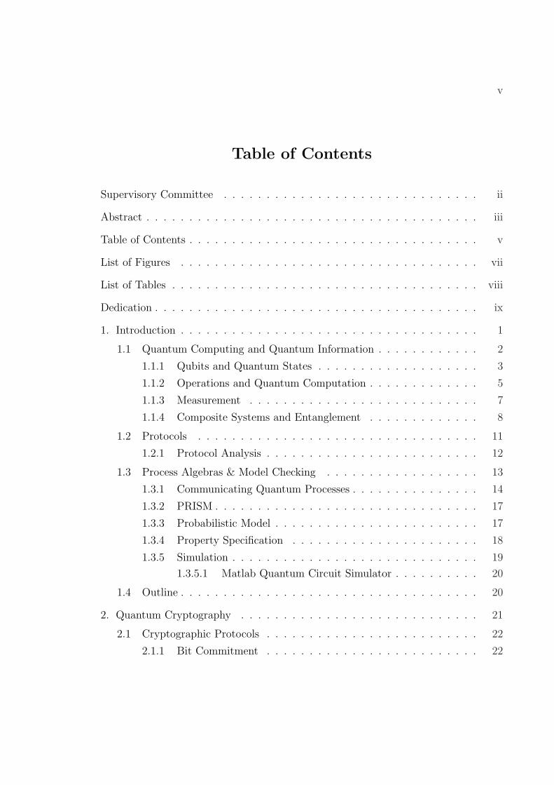
3.1 Property Verification: Honest Case . . . . . . . . . . . . . . . . . . . . 42

3.2 Property Verification: Dishonest Case . . . . . . . . . . . . . . . . . . . 43

4.1 Stochastic Results for Dishonest B . . . . . . . . . . . . . . . . . . . . . 63

4.2 Robust Results for Dishonest B . . . . . . . . . . . . . . . . . . . . . . 63

4.3 Quantitative Results for Dishonest A . . . . . . . . . . . . . . . . . . . 65

4.4 Dishonest A vs dishonest B . . . . . . . . . . . . . . . . . . . . . . . . . 65

ix

Dedication

To my parents, for their continued support and encouragement

Chapter 1

Introduction

Cryptography is the art and science of secure communications, whether it be keeping

information secret from an adversary or the problem of communicating between two

or more mistrustful parties. While cryptography dates back to the Babylonians and

has had historic military use, from the Caesar cypher used by Julius Caesar to com-

municate with his generals to the Enigma machine famously cracked by Alan Turing

during World War II, it is now used in a broad range of commercial and public ap-

plications from talking on cell phones to online shopping. Research and development

in cryptography has never been more important than in this age of communications

and information management.

A significant advance in the cryptographic field has been the introduction of Quan-

tum Computing, the study of computation that can be performed using quantum

mechanical systems, as opposed to the classical computing of our modern digital

computers that can be described with classical physics (mechanics, electromagnetism

etc.). While quantum mechanics was proposed and developed throughout the early

and middle 1900’s, it was only applied to large scale quantum systems (those con-

taining an enormous number of individual quantum systems) such as in the study of

superconductivity. It was not until the later half of the century that there was inter-

est in the more difficult problem of obtaining complete control over a single quantum

system. In 1982 two foundations were laid; first Benioff showed that quantum systems

could efficiently simulate classical computation [3], and second, Feynman showed the

converse is not true and that the number of variables required to describe a quantum

system grow exponentially with its size and can not be efficiently simulated with a

2

classical computer [17]. The proposed solution to this was the quantum computer, or

the universal quantum simulator.

The idea of quantum computing lends itself to cryptography in two ways: first

the laws of quantum mechanics ensure a certain level of protection from quantum

information being intercepted, and second the potential increase in computational

ability threatens some aspects of current cryptography that rely on hard mathematical

problems. As such, the development of quantum computing directly affects the field

of cryptography as advances in research push new ideas for processes and protocols

to improve communications and information security.

The rest of this chapter will introduce quantum computing and protocol analysis

in relation to the design and implementation of a quantum cryptographic primitive

we review in Chapter 2.

In the following two chapters we will take a closer look at quantum computing and

how it is related to the design and implementation of some cryptographic primitives.

1.1 Quantum Computing and Quantum Information

The field of quantum computing mixes the fundamentals of computer science with

the laws of quantum mechanics. As a classical computer must be able to compute

and communicate classical data, a quantum computer must be able to do likewise,

that is manipulate and communicate quantum information. Analogous to classical

computing, quantum computers have similar building blocks: quantum bits to store

information and quantum gates to manipulate information. In addition, quantum

computers have additional capabilities inherited from quantum mechanics. These

include superposition, the ability of a quantum bit to not just be 0 or 1, but some

combination of these values, and entanglement, the correlation quantum bits can have

with each other even at a distance.

3

Following is a brief introduction to Quantum Computing and Quantum Informa-

tion, focused around four fundamental postulates of quantum mechanics [22][32].

1.1.1 Qubits and Quantum States

The quantum bit (or qubit) is the basic building block of the quantum computer,

analogous to the bit in classical computing. Like the classical bit, the qubit can

have a state, |0〉 or |1〉, but unlike the classical bit, the qubit can also be in a linear

combination of states:

|ψ〉 = α|0〉+ β|1〉 (1.1)

where α, β ∈ C, and |α|2 + |β|2 = 1.

The state |ψ〉 is in a combination of states |0〉 and |1〉, but will collapse to just

one of these, upon observation or measurement, with some probability based on the

amplitudes α and β (see section 1.1.3). This combination of states, or superposition,

is key to realizing the power of quantum computation.

Definition 1.1.1. An inner product is a function which takes two vectors as input

and produces a complex number as output.

((ν1, . . . , νn), (ω1, . . . , ωn)) =∑

i

νi∗ωi

where ν∗ is the complex conjugate of ν.

Definition 1.1.2. A finite dimensional Hilbert space is an inner product space,

that is a vector space where all vector pairs have an inner product.

Postulate 1: Associated to any isolated physical system is a complex

vector space with inner product (that is, a Hilbert space) known as the

state space of the system. The system’s state is completely described by

its state vector, which is a unit vector in the system’s state space.

4

Mathematically a qubit is a unit vector in a two dimensional complex vector space.

We represent this vector using Dirac’s braket notation [16]

Definition 1.1.3. Braket notation, also known as Dirac notation, is a convenient

way of expressing vectors in quantum mechanics. The notation is composed of two

components, the “bra” 〈ω| and the “ket” |υ〉. The more common component is the

ket, which is a vector, written as a column vector:

|υ〉 =

υ1

υ2

...

υn

The bra component is the vector dual, 〈υ| = (|υ〉)†, where † denotes the adjoint of

the vector, taken by first transposing and then taking the complex conjugate:

〈υ| =(

υ1∗ υ2

∗ . . . υn∗

)

The full braket notation 〈ω|υ〉 is the scalar product, or inner product, of the two

vectors. While the reverse notation 〉ω|υ〈 is the outer product of the vectors.

With braket notation defined we can add vector representation to Equation 1.1

|ψ〉 = α|0〉+ β|1〉 =

α

β

(1.2)

which, when either α or β are 0, leads us to the states

|0〉 =

1

0

and |1〉 =

0

1

(1.3)

5

which are known as the standard, or computational basis states, and form an or-

thonormal basis for this vector space. Two more important states

|+〉 =1√2|0〉+

1√2|1〉 =

1√2

1√2

(1.4)

and

|−〉 =1√2|0〉 − 1√

2|1〉 =

1√2

− 1√2

(1.5)

are known as the dual, or diagonal basis states, which when measured with respect

to the computational basis, yields result |0〉 with probability | 1√2|2 = 1

2and result |1〉

with probability | ± 1√2|2 = 1

2.

In fact a set of basis states can be defined as any set of vectors that form an

orthonormal basis for a vector space.

1.1.2 Operations and Quantum Computation

Quantum computation is the change of a quantum state by applying a quantum

operation.

Definition 1.1.4. A unitary matrix is a complex matrix U that satisfies the con-

dition U †U = I, where U † is the adjoint of U , obtained by transposing U and then

taking its complex conjugate.

Similar to classical computation, operations are enacted by gates, and a quantum

gate is transformation, represented by a unitary matrix U , applied to a state space

|ψ〉. The unitary property preserves the basic qubit conditions found in Equation 1.1.

Postulate 2: The evolution of a closed quantum system is described by

a unitary transformation. That is, the state |ψ〉 of the system at time t1

6

is related to the state |ψ′〉 of the system at time t2 by a unitary matrix U

which depends only on the times t1 and t2

|ψ′〉 = U |ψ〉. (1.6)

Let us look at the quantum NOT gate, which, similar to the classical NOT oper-

ation, will change the pure state |0〉 to |1〉 and vice versa.

X =

0 1

1 0

(1.7)

In fact, the quantum NOT operation works on any qubit state and effectively switches

the amplitudes, such that α|0〉+ β|1〉 becomes α|1〉+ β|0〉 as shown here

X|ψ〉 =

0 1

1 0

·

α

β

=

β

α

(1.8)

A quantum gate without a classical counterpart is the Hadamard, or H gate. One

of the most useful single qubit operations, the H gate, defined as

H =1√2

1 1

1 −1

(1.9)

maps |0〉 ↔ |+〉 and |1〉 ↔ |−〉, changing pure basis states to diagonal basis states

and vice-versa.

H|0〉 =1√2

1 1

1 −1

·

1

0

=

1√2

1√2

= |+〉 (1.10)

and

H|1〉 =1√2

1 1

1 −1

·

0

1

=

1√2

− 1√2

= |−〉 (1.11)

Quantum gates can operate on more than one qubit as well. For example a

Controlled-U operation is a two qubit operation with a control bit and a target bit.

7

If the control bit is 1 then the operation U is applied to the target bit, otherwise the

target bit is left alone. The most common controlled operation is the Controlled-NOT

(CNOT) operation, defined as

CNOT =

1 0 0 0

0 1 0 0

0 0 0 1

0 0 1 0

(1.12)

1.1.3 Measurement

We have seen how a qubit can be in a potentially infinite number of superpositions

of states, however superpositions cannot be discretely measured. When a quantum

system is measured, or observed, it collapses to a pure basis state with some proba-

bility. Given a single qubit system α|0〉 + β|1〉, measurement on the standard basis

(|0〉, |1〉) will yield result |0〉 with probability |α|2 and |1〉 with probability |β|2, and

leave the system in the value of its result.

Postulate 3: Quantum measurements are described by a collection Mm

of measurement operators. These are operators acting on the state space

of the system being measured. The index m refers to the measurement

outcomes that may occur in the experiment. If the state of the quantum

system is |ψ〉 immediately before the measurement then the probability

that result m occurs is given by

p(m) = 〈ψ|M †mMm|ψ〉, (1.13)

and the state of the system after the measurement is

Mm|ψ〉√〈ψ|M †

mMm|ψ〉(1.14)

8

The measurement operators must satisfy the completeness equation

∑m

M †mMm = I (1.15)

which ensures that the sum of the probabilities p(m) is equal to 1. Note that all

basis states satisfy the completeness equation and therefore make valid measurement

operators.

Example 1.1.5. Measure state |+〉 in the computational basis. From the computa-

tional basis we get measurement operators {M0,M1} where Mi∈0,1 = 〈i|i〉. Then from

Equation 1.13 we have

p(1) =(

1√2

1√2

)· 0 0

0 1

·

0 0

0 1

·

1√2

1√2

=

1

2

and

p(0) =(

1√2

1√2

)· 1 0

0 0

·

1 0

0 0

·

1√2

1√2

=

1

2

Therefore the probabilities of getting result 0 or 1 are both 12.

1.1.4 Composite Systems and Entanglement

Multiple qubit state vectors can be combined together to create a state space

which describes a quantum system. The size of the state space grows with the size of

the cartesian product of its state vectors, therefore, a quantum system of n qubits is

a unit vector in a 2n dimensional complex vector space.

Definition 1.1.6. The tensor product is a way of combining vector spaces to form

a larger vector space. For our purposes we will only consider vectors and matrices

of finite dimension, and so the definition of a tensor product simplifies to the outer

product (for vectors), and the kronecker product (for matrices).

9

Postulate 4: The state space of a composite physical system is the ten-

sor product of the state spaces of the component physical systems. More-

over, if we have systems numbered 1 through n, and system number i

is prepared in the state |ψi〉, then the joint state of the total system is

|ψ1〉 ⊗ |ψ2〉 ⊗ · · · ⊗ |ψn〉.

This gives us the tensor product as a tool to combine quantum state spaces to-

gether into a single system.

Definition 1.1.7. We use the terms A and B to represent the different parties during

two party communications.

Example 1.1.8. Let A and B each have a pure quantum state, |0〉 and |1〉 respectively.

Then we could describe the total system of A and B together as

|0〉 ⊗ |1〉 =

1

0

⊗

0

1

=

0

1

0

0

= |01〉.

A general case two qubit system similar to the general single qubit system in

Equation 1.1 is

|ψ〉 = α00|00〉+ α01|01〉+ α10|10〉+ α11|11〉 =

α00

α01

α10

α11

(1.16)

where α00, α01, α10, α11 ∈ C, and α200 + α2

01 + α210 + α2

11 = 1.

10

We see in Equation 1.16 that if we set any of α00, α01, α10, α11 = 1 we get one of

the four possible pure states, or basis states. Alternatively, by measuring the system

on the computational basis we will also end up with a pure state |00〉, |01〉, |10〉, or

|11〉 with probabilities |α00|2, |α01|2, |α10|2, and |α11|2 respectively.

Similarly some states can be decomposed into separable state vectors. Take the

final state in Example 1.1.8, |01〉, which can be separated into the states |0〉 and |1〉.Now consider the two qubit state |ψ〉= |00〉+|11〉√

2. We can show that |ψ〉 cannot be

expressed in terms of composite states as there are no single qubit states |a〉 and |b〉such that |a〉⊗|b〉=|ψ〉.

Proof Sketch. Assume |ψ〉 can be expressed as a product of two composite states.

Then

|ψ〉 = |a〉 ⊗ |b〉

=

a1

a2

⊗

b1

b2

=

a1b1

a1b2

a2b1

a2b2

=

1√2

0

0

1√2

which upon inspection has no solution.

Definition 1.1.9. When a system cannot be written as a product state of its compo-

nent systems, it is said to be in an entangled state.

The most common entangled states are the four Bell states (also referred to as

EPR states or EPR pairs), named after some of the people who first pointed out

their properties: Bell, Einstein, Podolsky, and Rosen. The Bell states are created

11

from the four computational basis states and applying first a Hadamard gate then a

Controlled Not gate, giving us:

|β00〉 =|00〉+ |11〉√

2(1.17)

|β01〉 =|01〉+ |10〉√

2(1.18)

|β10〉 =|00〉 − |11〉√

2(1.19)

|β11〉 =|01〉 − |10〉√

2(1.20)

Entangled states have the interesting property that by observing any qubit in the

state, there is an immediate effect of determining the value of the other qubits. This

is true no matter how far apart they are and if the qubits are physically separated;

we call this the non-local effect [2].

Example 1.1.10 (EPR Paradox). Consider the 2 qubit Bell state |β01〉 (Equation

1.18). Then let A and B each take half of the state (a single qubit) and separate them

by some distance. WLOG let B measure his half of the state giving him result |0〉, he

then immediately knows that A’s half of the state is |1〉, regardless of whether A has

measured her half yet or not.

1.2 Protocols

We define a protocol as a series of steps with associated rules and actions that

govern the communications between two or more parties working to achieve an explicit

goal. The protocol’s steps must have a sequence; that is, there must be an initial and

a final step and each step must complete before the next step is executed. Each step,

rule, and action must be: firstly, well defined, so that they are unambiguous and there

is no chance of misunderstanding; and secondly, known and agreed, in advance, to all

12

parties involved in the protocol. An example protocol is a Coin Flipping game, which

involves two parties where one party will flip a coin, and depending on the results

there is an agreed upon winner.

A cryptographic protocol is a protocol that includes steps to secure the commu-

nications between the parties. Typically this will address security concerns such as:

the involved parties trust each other and require that the protocol is secure from a

third party eavesdropper, or the parties do not trust each other and require that the

protocol is secure against one of them acting dishonestly. We use the term secure

in the probabilistic sense, that is, it addresses these concerns within some arbitrar-

ily small probability of error. Furthermore, we can say a cryptographic protocol is

unconditionally secure if it is secure against an adversary with unlimited computing

power, and computationally secure if it is secure against an adversary with currently

available (modern day) computing power.

For the two party protocols discussed in this thesis we will use the conventional

naming practice, Alice and Bob (represented by A and B respectively), for the in-

volved parties; where A will typically initiate the protocol and B will respond.

While a great deal of research goes into developing new protocols, it is equally

if not more important to conduct analysis on existing protocols, either to prove a

protocol is secure, improve the bound of error on its security, or prove a protocol

insecure therefore leading to potential improvements.

1.2.1 Protocol Analysis

The formal analysis of cryptographic protocols has been driven from the desire of

researchers to prove protocols secure.

There are four basic approaches to the analysis of cryptographic protocols [30][34]:

1. Model and verify the protocol using specification languages and verification

tools not specifically designed for the analysis of cryptographic protocols.

13

2. Develop expert systems that a protocol designer can use to develop and inves-

tigate different scenarios.

3. Model the requirements of a protocol family using logic for the analysis of

knowledge and belief.

4. Develop a formal method based on the algebraic term-rewriting properties of

cryptographic systems.

The first two approaches are useful for proving specific properties of a protocol

or determining if the protocol contains a given flaw, but they are not guaranteed to

identify all flaws and do not prove security of a protocol. The third approach gained

wide popularity with the introduction of Burrows-Abadi-Needham logic [10], or BAN

logic, and while it has a simple intuitive set of rules making it easy to use, it has

demonstrated serious flaws in protocols. The fourth approach models a cryptographic

protocol as an algebraic system and analyzes the attainability of certain states to show

that a protocol meets its requirements.

State exploration tools are generally stronger than belief logics as they have a lower

level of abstraction, and in our case they are better able to model the probabilistic

nature of quantum computing. Therefore it is this fourth approach that we will be

applying in the modeling and analysis of our quantum cryptographic protocols.

The following sections briefly describe the tools we use for this approach in Chapter

3.

1.3 Process Algebras & Model Checking

We define a process algebra as the use of algebraic laws or axioms to study the

behavior of concurrent systems. It is a tool that allows us to specify these systems as

a number of interacting processes and reason about them using algebraic equations,

14

typically for the purpose of analysis or verification.

While there are a number of process algebras in use with varying sets of rules and

purposes, there are a few features that are common to them all. First is process in-

teraction, where communications between processes happens through channels rather

than shared variables. Secondly, processes are described from a small set of primitive

operators defined by the operational semantics of the process algebra. And finally,

a defined set of algebraic laws that use the set of operators to build and manipulate

expressions.

Model Checking is a method of automatic analysis of these systems used to find

subtle errors or design flaws in the system specification. A model checker usually

takes two inputs, a description of the system to be modeled and a set of properties

that should hold for the system. Process algebras give us a formalized mathematical

framework in which to describe the system of a protocol in a language that can be

used as input to a model checker. The properties expected to hold for a protocol are

most naturally formulated as temporal logic statements.

1.3.1 Communicating Quantum Processes

Communicating Quantum Processes (CQP) is a process algebra that combines

the communication primitives of pi-calculus [31] with quantum primitives for the

transformation and measurement of quantum states. It was created by Simon Gay

and Rajagopal Nagarajan [18] to model systems that have both quantum and classical

communications or computation, such as cryptographic protocols. Initially intended

to model and verify an end-to-end implementation of the BB84 protocol, we will use

the language to formalize the description of a quantum cryptographic primitive in

Chapter 3.

We define the syntax of CQP by the grammar in Figure 1.1, and will describe each

component: types, values, expressions and processes in more detail in the rest of this

15

T ::= Int | Unit | Qbit |[T ] | Op(1) | Op(2) | . . .

v ::= 0 | 1 | . . . | unit | H | . . .

e ::= v | x | measure e | e∗ = e | e + e

P ::= 0 | (P |P ) | e?[x : T ].P | e![e].P | {e}.P | (new x : T )P | (qbit x)P

Figure 1.1: Syntax of CQP

section. For a formal definition that includes internal syntax, operational semantics

and type system, see Gay and Nagarajan’s publication [18].

Types

Types T indicate the kind of data or structure that expressions and values may

contain, as well as the allowable operations or actions. At the basic level we have data

types which consist of primitive types such as Int and Unit (others can be defined), as

well as more complex data types like Qbit for qubits. More advanced types consist of

channel types [T1, . . . , Tn] where each message in the channel is an n-tuple (written

as T ) with component types T1, . . . , Tn, and unitary operator types Op(n) that apply

some unitary operation Op on n qubits.

Definition 1.3.1. The primitive data type Unit has only one value, the constant unit,

used as a filler for uninteresting arguments and results (similar to Void or Null in

some languages). There are no operations on Unit, but there are rules that state Unit

is a legal type and unit is a legal value of Unit. [11]

Values

Values v are a specific piece of data or meaning classified by some data type. Values

can be literal values of data types such as 0, 1, . . . for Int, unit for Unit, and |0〉, |+〉for Qbit, as well as composite values of unitary operator types such as H (Hadamard

16

operator) and X (Not operator).

Expressions

Expressions e consist of values, variables (x,y,z etc.) and operations that can be eval-

uated according to the rules defined by the operational semantics. Operations consist

of measurements measure e1, . . . , en, applications of unitary operators e1, . . . , en∗ = e,

and expressions involving data operators such as e + e′.

Processes

Processes P are the highest level descriptor of a system; they define behavior and

interaction of a system’s component parts. Processes end and branch with the null

(terminated) process 0, and the parallel composition P |Q of processes respectively.

Interaction between processes consists of inputs e?[x : T ].P , where input-bound vari-

able x of type T is received on e, and outputs e![eo].P , where output expression eo is

sent on e. For both inputs and outputs the expression e is constrained by the type

system to refer to a channel. Process actions {e}.P define the inclusion of expressions

into our system. A typical action is the application of a unitary operator, for exam-

ple the application of a Hadamard operator to a qubit variable {x∗ = H}. Finally,

processes can create new variables of any valid type, such as channel declarations

(new x : T )P and qubit declarations (qbit x)P

Example 1.3.2. Consider a simple transmit process where A sends a single qubit to

B, modeled as follows in CQP.

Transmit = (new s :[Qbit])(Alice(s) | Bob(s))

Alice(s :[Qbit]) = (Qbit x)(s![x].0)

Bob(s :[Qbit]) = s?[y : Qbit].0

17

At the top level the Transmit process creates a new qubit channel s, then starts

processes A and B in parallel, both with parameter s. The process A creates a new

qubit x, sends x out on channel s, then terminates, while process Bob waits for an

incoming qubit, which he refers to as y, and once it is received he terminates.

1.3.2 PRISM

PRISM is a probabilistic model checker used to model and analyze systems with

probabilistic behavior. As the result of a qubit measurement is a probabilistic dis-

tribution of the amplitudes of the measurement basis, PRISM is able to model this

behavior as part of an overall quantum system.

There are two stages to the PRISM approach. First is to model the system in the

PRISM language such that all states and transitions of the system are represented.

The second is to formally express properties of the system with a temporal logic to

be analyzed against the PRISM model. By running the temporal logic statements

against the PRISM model we can verify whether or not they hold and with what

probability they hold for the system.

Full descriptions and instructions for both stages can be found in the PRISM

Users’ Guide [33]; however, we will briefly summarize the main components of both

the modeling language, and the temporal logic used to specify the model’s properties.

1.3.3 Probabilistic Model

The type of model we will use in PRISM is the discrete-time Markov chain

(DTMC). The DTMC consists of a finite set of states S, a set of initial states S ⊆ S,

and a transition probability matrix P : S × S → [0, 1]. For each pair of states s, s′

we give the probability of making the transition from s to s′ as P(s, s′), and require

that∑

s′∈S P(s, s′) = 1 for all states s ∈ S. Terminating states can be modeled by

adding a self-loop, that is setting P(s, s) = 1.

18

A PRISM model consists of a number of modules, which are processes that can

interact with each other. A module contains local variables, which at any given

time constitute the state of the module, and a set of commands, which describe the

behavior of the module. Commands take the form:

[]g → λ1 : µ1 + . . . + λn : µn; (1.21)

where the guard g is a predicate over all variables in the model, update µi is a transi-

tion the module can make if the guard is true, and expressions λi assign probabilistic

distributions to the transitions. Transitions are specified by assigning new values to

one or more variables, thus changing the state of the module.

1.3.4 Property Specification

Properties in PRISM are specified using a language based on the temporal logic

PCTL [5][23], a probabilistic extension to the classic temporal logic CTL. The basic

syntax of the language used to express the properties we need is defined in Figure

1.2, where:

• 〈expr〉 is a PRISM language expression which evaluates to a Boolean,

• 〈op〉 is a relational operator (one of <, <=, >= or >),

• 〈p〉 is a PRISM language expression evaluating to a double (real number) in the

range [0,1],

• 〈prop1〉 U 〈prop2〉 is the “Until” path property which is true if 〈prop1〉 is true

until 〈prop2〉 is true.

There are two types of properties used in our model. The first is an assertion

where the outcome is true or false and will look like

P >= 1 [ true U cheat detected ]

19

〈prop〉 ::= true | false | 〈expr〉 |!〈prop〉 |〈prop〉 & 〈prop〉 |〈prop〉 => 〈prop〉 |P〈op〉〈p〉 [ 〈pathprop〉 ]

〈pathprop〉 ::= 〈prop〉 U 〈prop〉

Figure 1.2: Syntax of PCTL

Which will return true if, with probability 1, the expression cheat detected eventually

resolves to true. The other type of property we define is one that evaluates to some

numeric value that corresponds to the probability of that property holding. For

example

P =? [ reveal stage & commit bit = 1 ]

returns the probability P that the model will enter a state such that the expression

reveal stage resolves to true and variable commit bit has the value 1.

1.3.5 Simulation

Quantum systems can also be analyzed through simulation. This is done by

developing the corresponding circuit as a series of quantum gates, then for some

input or initial state, the circuit can be run and a corresponding output or final state

is given. For a finite set of inputs a circuit simulator can give us the outputs to

check against the expected results of a protocol. While a model checker is used to

analyze states within a protocol, the circuit simulator is used to analyze values of

qubits within these states.

20

1.3.5.1 Matlab Quantum Circuit Simulator

The quantum circuit simulator used in this thesis was developed, by the author,

in Matlab as a tool to help check quantum states and transitions [39]. The simulator

takes an input vector that represents the input state, applies a transformation matrix

which is the product of all operations (or gates) in the circuit, and outputs a vector

which represents the final state. An n-bit quantum state can be represented by

a 2n × 2n matrix, however as this requires memory exponential to the size of the

number of qubits, we can only simulate small quantum systems.

1.4 Outline

In Chapter 2 we will introduce quantum cryptography and review related research

that has been completed to date on both quantum cryptographic primitives and the

tools used in their analysis. Chapter 3 will propose our formal approach to the

modeling and analysis of quantum cryptographic primitives as well as detail the tools

and methods we have developed. Chapter 4 will follow the application of our formal

approach to a selected protocol and detail the results. Finally Chapter 5 will conclude

our research and propose future work.

21

Chapter 2

Quantum Cryptography

Quantum Cryptography is the implementation of secure communications and cryp-

tographic protocols based on the laws of quantum mechanics. Initially introduced by

Stephen Wiesner with his multiplexing primitive [40](a quantum implementation of

oblivious transfer), the concept was greatly expanded by Bennett and Brassard with

the BB84 quantum key distribution and quantum coin flipping protocols [4]. BB84

effectively allowed an unconditionally secure (by the laws of quantum mechanics)

method for the distribution of a random bit string over a quantum channel. Over

the next decade a number of algorithms and protocols were developed and enhanced,

most notably of which was Shor’s algorithm, which could efficiently factor prime num-

bers and find discrete logs [35]. This had huge implications, as the assumed hardness

of factoring prime numbers and finding discrete logs is what the security of current

Public Key Cryptography (eg RSA) is based on. If quantum computing could break

classical cryptography, could we then provide a new quantum cryptographic approach

that was secure against an adversary with a quantum computer? Shor’s discovery pro-

pelled quantum cryptography into a rapidly developing field and opened it to a much

larger audience. Shortly after this period IBM built and tested the first quantum

computer [38]. A five qubit machine that was able to demonstrate an order-finding

algorithm with the same structure as Shor’s algorithm.

Today quantum cryptography has a large and vibrant research community working

on a broach range of topics from theoretical protocols to physical experiments on

qubits. Due to the success of the BB84 protocol, a major area of current research

is in quantum communications and in increasing both the distance possible and the

22

reliability of qubit states.

2.1 Cryptographic Protocols

We define a cryptographic protocol as a method for two parties, A and B, to

perform computations involving data that they want to keep secret from each other.

We define cryptographic primitives as building blocks to constructing cryptographic

protocols [13].

The primitives that we will look at are: Bit Commitment and Oblivious Transfer.

2.1.1 Bit Commitment

Bit Commitment is a cryptographic primitive involving two mistrustful parties,

A and B, where A seeks to commit to a bit such that B is unable to learn the bit

before it is revealed (sealing property) and A is unable to change the bit once it has

been committed (binding property).

An example protocol would be A writes the bit down on a piece of paper and

locks it in a lockbox. She then passes that lockbox to B while retaining the key. This

process is binding as A cannot change her bit without getting into the safe (which is

in B’s ownership) and is sealing as B cannot get into the safe without A’s key.

Bit commitment is a fundamental primitive that has been a useful tool in the

implementation of numerous cryptographic protocols, most notably coin tossing [6]

and zero-knowledge proofs [20][21].

2.1.2 Oblivious Transfer

Oblivious Transfer is a cryptographic primitive where A sends a bit to B in such

a way that B receives the bit with 50% probability. B knows whether he received the

bit, while A obtains no information on whether the transfer was successful.

23

An important application of oblivious transfer is in building secure multiparty

computation [12][14][19][25][42].

2.2 Quantum Bit Commitment

Quantum Bit Commitment

Assume that A wishes to commit a bit b to B. Let s be a security parameter.

commit stage

1. A chooses a vector of s random bits B. Each bit is then encoded in the

standard or diagonal basis, standard if b = 0 and diagonal if b = 1. Finally, Asends the resulting sequence of s encoded bits to B.

2. B chooses a random basis (standard or diagonal) to measure each incoming

bit, and records the result into two tables — one for the standard basis and

one for the diagonal.

unveil stage

1. A reveals to B the committed bit b and the unencoded sequence of bits B.

2. B verifies A’s claim by comparing his records in the table for the basis corre-

sponding to b — standard if b = 0 and diagonal if b = 1. There should be

perfect agreement with entries in that table and no correlation with the other

table.

Figure 2.1: The BB84 Quantum Bit Commitment Protocol.

The first published quantum bit commitment protocol (QBC) is from Bennett

and Brassard’s BB84 paper [4]; while the paper itself contained a Quantum Key

24

Distribution and Quantum Coin Flipping protocol, the latter is easily modified to

QBC (see Figure 2.1). The protocol, however, is susceptible to entanglement based

cheating by A. Let A prepare s pairs of entangled bits in the state 1√2([01〉 + [10〉),

then for each state send one half to B and store the other half. When A is ready

to unveil, she measures her bits in the standard basis to commit to b = 0 and the

diagonal basis to commit to b = 1.

The next major development in quantum bit commitment was the BCJL93 [8]

protocol (see Figure 2.2), an improvement on a previous protocol BC91 [7]. Initially

believed to be unconditionally secure, this protocol was later shown to be susceptible

to the same type of entanglement attack as BB84 [28][26]. In fact, during this time

it was put forward that unconditionally secure QBC may not exist.

2.2.1 The No-Go Theorem

The impossibility of unconditionally secure quantum bit commitment, sometimes

referred to as the no-go theorem, was put forward independently by Lo and Chau

[26][27] and Mayers [28][29], and later summarized by Brassard, Crepeau, Mayers,

and Salvail [9]. Initially these were attacks on the BCJL93 protocol showing that it,

and all proposed QBC protocols at the time, were in fact susceptible to the same

EPR attack as BB84. However both claims were later generalized to include all QBC

protocols.

The general idea behind the no-go theorem is that any sealing QBC is necessarily

non-binding. The proof sketches as follows [15]. At the end of the commitment phase,

B will hold one of two quantum states %k for A’s commitment to k ∈ 0, 1. A holds

the purification for this state ψk which she will pass to B during the unveil phase. For

the protocol to be sealing, the two states %k need to be indistinguishable, then from

Uhlmann’s theorem [32][37], there exists a unitary transformation U that rotates the

purification of %0 to %1. Since U is localized to the purification systems only, which

25

are under A’s control, then A is able to switch %k back and forth between %0 and %1

at will, and is therefore not bound to her commitment.

Bounds to the no-go theorem were provided by Spekkens and Rudolph [36] who

looked at degrees of concealment and bindingness that can be achieved simultaneously

in a QBC.

With the advent of the No-Go theorem it is generally accepted that uncondi-

tionally secure quantum bit commitment, and therefore perfectly fair quantum coin

flipping, is impossible. As such, a number of research avenues have opened up in devel-

oping protocols that rely on restrictions to memory, or measurements, or relativistic

location. Another research focus is on the tradeoffs of bindingness and concealment

and bounding the bias of a cheating adversary.

2.2.2 Cheat Sensitive Quantum Bit Commitment

We define a class of cryptographic protocols as cheat sensitive if they guarantee

that if one party cheats, the other will detect the cheating with some probability

strictly greater than zero.

Cheat sensitive quantum bit commitment was introduced simultaneously and in-

dependently by Hardy and Kent [24] and Aharonov et al. [1]. The main idea is to

encode the BC in non-orthogonal states such that if either side tries to extract infor-

mation, they disturb the state and therefore risk detection. Hardy and Kent propose

a protocol where both sides are simultaneously at risk of cheat detection by adding

an entangled singlet state that effectively randomizes which side ends up with the

encoded commit bit, and is therefore able to check for cheating. Figure 2.3 outlines

the protocol and we follow up with a more detailed description in the next chapter.

Hardy and Kent’s protocol is interesting in that it can simultaneously detect

cheating by either party; however the authors only prove that the probability of

detection is nonzero. In the next chapter we will use this protocol as an example of

26

our modeling and analysis methodology, verify the nonzero probability of detection

property, and put quantitative bounds on the cheat detection for both a dishonest Aand a dishonest B.

27

Quantum Bit Commitment Revisited

commit stage

1. B chooses a Boolean matrix G as the generating matrix of a binary linear

(n, k, d)-code C such that the ratio d/n > 10ε and the ratio k/n = 0.52 and

announces it to A.

2. A chooses a random binary vector r of length n and announces it to B.

3. A chooses a random k-bit vector s, such that r · c = x, where c = sG.

4. A chooses a random sequence b of length n of the polarizations, B or D, and

sends to B a sequence of n photons with the polarization of the ith photon

Pbi(ci), where P0(0) = 0◦, P0(1) = 90◦ and P1(0) = 45◦, P1(1) = 135◦.

5. B chooses a random string b′ of n bits and measures the ith photon according

to the basis M(b′i), where M(0) = B and M(1) = D. Let c′ be the n-bit vector

where c′i is the result of the measurement of the ith photon.

unveil stage

1. A sends c,b and x to B.

2. B verifies that c is a codeword of C and computes B =∑

i|b′i=bi

ci⊕c′in/2

, in order

to verify that the error rate is under the limit of those pairs of outgoing and

measured bits that were polarized/measured by the same basis.

3. if B < 1.3ε and x = r · c, then B accepts, otherwise B rejects.

Figure 2.2: The BCJL93 Quantum Bit Commitment Protocol.

28

Cheat Sensitive Quantum Bit Commitment

1. Stage 0: the prelude. B prepares a singlet state, |Ψ−〉AB = 1√2(|0〉A|1〉B −

|1〉A|0〉B), and sends qubit A to A.

2. Stage 1: the commitment. The protocol allows a simple commitment proce-

dure which A may use if she wishes to commit to a definite classical bit: to

commit to 0, she prepares a qubit C chosen randomly to be either |0〉 or |−〉,each with probability 1/2; to commit to 1, she similarly prepares either |1〉 or

|+〉. Then she sends the C qubit to B.

3. Stage 2: the unveiling. A is first given the option of challenging the singlet.

If she does and it fails the test, she has detected cheating. Next, whether or

not she made a challenge, she must reveal the value of the committed classical

bit. B then has the option of challenging the singlet, if A did not. If he does

and the singlet fails the test, he has detected cheating.

4. Stage 3: the game. If either party earlier challenged the singlet, they automat-

ically lose the game. If neither challenged the singlet, they now each measure

their singlet qubit in the |0〉, |1〉 basis. B sends his results to A. If hers is not

opposite, she has detected cheating.

If B reports the result 1 then A loses the game; if 0 then B loses. If A loses

then she reveals the encoding state for C, and if B loses he returns C to A.

This allows the winning party to examine C for signs of cheating.

Figure 2.3: Cheat Sensitive Quantum Bit Commitment Protocol.

29

Chapter 3

Modeling and Analysis

Given a quantum cryptographic protocol our goal is to verify its correctness in the

presence of cheating, and to quantify the bounds of a dishonest party member’s

ability to cheat the protocol, along with the bounds of such cheating being detected.

By identifying a maximum cheat strategy we have identified key steps within the

protocol that may be able to be strengthened.

We will define a formal approach to this task as follows:

1. Formalize the protocol’s description in the process algebra CQP.

2. Model the formalized protocol in the probabilistic model checker PRISM.

3. Verify the protocol model in PRISM with the temporal logic PCTL.

4. Analyze quantum cheat strategies to find optimal values to add to our PRISM

model in the case of a dishonest party.

3.1 The Protocol

The protocol we will consider is a Cheat Sensitive Quantum Bit Commitment

[24]. Here A will commit a bit to B; at the completion of the protocol if either

party attempted to cheat the binding or sealing property then there is some positive

probability that the other party will detect such cheat attempt. We will summarize

the protocol as follows:

Stage 0: the prelude. B prepares a singlet state

|Ψ−〉AB =1√2(|0〉A|1〉B − |1〉A|0〉B) (3.1)

30

and sends qubit A to A. At various points in the protocol the singlet state may

be challenged, where the challenger receives the other party’s half of the state and

measures them to confirm values of 01 or 10. Any variation from these values implies

that the singlet state has been modified and therefore cheating has been detected. If

neither party challenges, the singlet is used to provide a random winner, who receives

the final qubit states and is able to check them for any signs of cheating.

Stage 1: the commitment. A commits to a definite classical bit c ∈ 0, 1: to

commit to 0 A randomly prepares qubit C as either |0〉 or |−〉 with equal probability.

Similarly to commit to 1 she prepares C as either |1〉 or |+〉. Qubit C is then sent to

B.

Stage 2: the unveiling. A has the option of challenging the singlet. If the

challenge fails then cheating is detected, otherwise no cheating is detected yet. Next

A must reveal her committed classical bit c. If A did not challenge the singlet then

B now has the option to do so, with a fail implying that cheating has been detected.

Stage 3: the game. If either party challenged the singlet then the other party

wins the game, otherwise A and B both measure their half of the singlet on the

standard basis and B sends his result to A. If Ameasured = Bmeasured then cheating is

detected, otherwise if B reports 1 then B wins and if he reports 0 then A wins.

If A loses then she must reveal the encoding state for C, B then measures C and

if Cmeasured 6= c, cheating is detected.

If B loses then he must return qubit C, A then measures C and if Cmeasured 6= c,

cheating is detected.

3.2 Formalize

The first step is to formalize the protocol in the language CQP so that we have

a consistent and correct model to work with. A formal description of the protocol

31

allows us to apply a set approach to the modeling and analysis, as well as lay the

framework for automated verification.

The conversion to CQP is a step by step approach of following each stage of the

protocol, identifying communicating channels (both inbound and outbound) and the

logical structure of the decisions made during the protocol. We create additional

classical bits and communication channels to manage party choice, for example to

communicate a binary decision or to terminate the process.

A protocol in CQP consists of a sequence of CQP processes as defined by the

syntax in section 1.3.1. We will review the key components of a CQP process here,

but first let us define the following variables: x as a data type, s as a channel type

with component type x, e as an operation expression, and b as a boolean expression.

Then the protocol can be defined as an overall process P that can be recursively

separated its component processes P1...n as P = Pi, i = 1 . . . n, where Pi is one of the

following process events:

1. {e}.Pi+1 – Process action: evaluate operation e then continue with process Pi+1.

2. s![x].Pi+1 – Process output: send data x along channel s then continue with

process Pi+1.

3. s?[x].Pi+1 – Process input: wait to receive data x from channel s then continue

with process Pi+1.

4. Pi+1|Pi+k – Process branch: continue with both processes Pi+1 and Pi+k, 1 <

k ≤ n− i, concurrently.

5. if b then Pi+1 else Pi+k – Process decision: if expression b evaluates to true then

continue with process Pi+1, otherwise continue with process Pi+k, 1 < k ≤ n− i.

6. 0 – Process end: terminate the current process.

32

All of the above process events are defined in section 1.3.1 except the process

decision, which we will define here.

For the operational semantics in our definitions we use the notation ¢ipi • ti =

p1 • t1 ¢ . . .¢pn • tn to denote a probability distribution∑

i pi = 1 over configurations

ti. Where a configuration t = (σ; φ; e|P ) consists of an expression or process and its

state information σ and φ (qubits and channels respectively)

Definition 3.2.1. A process decision is a process that, given a boolean expression b

and processes P and Q, will evaluate b = 1 and if the evaluation is true will continue

with process P otherwise it continues with process Q. We define the syntax for a

process decision as

P ::= if b then P else Q

with operational semantics defined by the reduction rule

(σ; φ; if b then P else Q) →e b • (σ; φ; P ) ¢ (1− b) • (σ; φ; Q) (R-Dec)

and the typing rule defined as

Γ ` b : Bool Γ ` P Γ ` Q

Γ ` if b then P else Q(T-Dec)

Similar to the process decision, we will also define a new operation expression

called the binary decision operation to give us decision making capability within an

operational expression e in a process action.

Definition 3.2.2. A binary decision (if-then-else) operation is an expression

that, given a boolean expression b and expressions e1 and e0, evaluates b = 1 and if

the evaluation is true it reduces to expression e1 otherwise it reduces to expression e0.

The syntax for the operation is defined as

e ::= if b then e1 else e0

33

with operational semantics defined by the reduction rule

(σ; φ; if b then e1 else e0) →e b • (σ; φ; e1) ¢ (1− b) • (σ; φ; e0) (R-If)

and the typing rule defined as

Γ ` b : Bool Γ ` e1 : T Γ ` e0 : T

Γ ` if b then e1 else e0

(T-If)

3.2.1 Conversion to CQP

We will now detail the protocol conversion to CQP by looking at each stage of the

protocol, breaking it into communication steps between A and B, each containing

a sequence of CQP processes, and follow it with a brief description of the actions

taken. The flowchart in Figure 3.1 gives a high level view of which protocol stages

are followed depending on whether there are challenges.

The complete results of the formalization of the protocol into CQP, which we de-

tail in the following steps, can be found in Appendix A.

Stage 0

B: {a∗ = H}.{a, b∗ = CNot}.s![a]

B creates an entangled pair by applying a Hadamard operation H to the

first qubit a, a Control Not operation CNot on both qubits a, b, then sends

half of the entangled pair a to A on channel s.

A: s?[a : Qbit]

A receives her singlet (half of the entangled pair) qubit a from B.

Stage 1

A: r?[d : Bit].r?[e : Bit].encode(d, e, c).s![c]

34

Figure 3.1: CSQBC Flowchart

35

A obtains two bits from the random bit generator channel r, the first is

her commit bit d and the second is her encoding basis e. She then encodes

her commit bit with the random basis and sends the resulting qubit c to

B.

B: s?[c : Qbit]

B receives A’s commit qubit c.

Stage 2 - Alice Challenges

A: t![x]

A sends her challenge bit x to B.

B: t?[x : Bit].s![b]

B receives A’s challenge bit x then sends his half of the singlet state b to

A.

A: s?[b : Qbit].if (measure a 6= measure b) then {w = 1}.t![w].t![d]

A receives B’s half of the singlet state b and measures it along with her

half of the singlet state a. If the measured singlet states are not equal (no

cheating detected) then A sets the winner bit w to B (since A challenged)

and sends it to him along with her commit bit d.

A: else {w = 0}.t![w].cheatdetected

If the measured singlet states are equal (cheating detected) then A sets

the winner bit w to herself, sends the bit to B then terminates the process

with cheatdetected.

36

Stage 2 - Bob Challenges

A: t![x].t![d]

A sends her no-challenge bit x and commit bit d to B.

B: t?[x : Bit].t?[d : Bit].t![y]

B receives A’s no-challenge bit x and commit bit d, then sends his chal-

lenge bit y to A.

A: t?[y].s![a]

A receives B’s challenge bit y and replies with her half of the singlet state

a.

B: s?[a].if (measure a 6= measure b) then {w = 0}.t![w]

B receives A’s half of the singlet state a and measures it along with his

singlet state b. If the measured singlet states are not equal (no cheating

detected) then B sets the winner bit w to A (since B challenged) and

sends it to her.

B: else {w = 1}.t![w].cheatdetected

If the measured singlet states are equal (cheating detected) then B sets the

winner bit w to himself, sends the bit to A then terminates the process

with cheatdetected.

Stage 2 - No Challenges

A: t![x].t![d]

A sends her no-challenge bit x and commit bit d to B.

37

B: t?[x : Bit].t?[d : Bit].t![y]

B receives A’s no-challenge bit x and commit bit d, then sends his no-

challenge bit y to A.

A: t?[y]

A receives B’s no-challenge bit y.

Stage 3 - Alice Challenges

B wins the game since A challenged the singlet state.

Stage 3 - Bob Challenges

A wins the game since B challenged the singlet state.

Stage 3 - No Challenges

Since neither party challenged the singlet state, a game is played to produce a

random winner w, where w = 0 ⇒ A wins, and w = 1 ⇒ B wins.

B: {w∗ = measure b}.t![w]

B measures his half of the singlet b and sends the result w to A.

A: t?[w].if (measure a 6= w) then t![1] else t![0].cheatdetected

A receives B’s measured half singlet w and compares it to her own half

singlet a. If they are not equal then A sends acceptance to B, otherwise

she sends reject to B and terminates the process with cheatdetected.

Alice Wins

B: s![c].done

38

B returns commit qubit c to A.

A: s?[c].{if e then c∗ = H else unit}.if (d = measure c) then done else cheatdetected

A receives her commit qubit c back from B, decodes it with encode bit e,

measures it and compares it to her original commit bit d. If they match

then she terminates the protocol successfully with done, and if they do

not match then modifications have been detected and she terminates the

protocol with cheatdetected.

Bob Wins

A: t![e].done

A reveals the encoding state e for her commit bit.

B: t?[e : Bit].{if e then c∗ = H else unit}.if (d = measure c) then done else cheatdetected

B receives encoding state e and uses it to decode A’s commit qubit c, then

measures c and compares it to A’s commit bit d. If they match then he

terminates the protocol successfully with done, otherwise modifications

have been detected and he terminates the protocol with cheatdetected.

3.3 Modeling

Once our protocol has been formalized in CQP, we want to model it in PRISM so

that we can run verification experiments on specific properties. The conversion from

CQP to PRISM here has been done for a subset of CQP by following an algorithm

where every CQP process step gets one or more PRISM commands. We define a set of

conversion rules in such a way that they could be used to automate the interpretation

from the formal CQP description to the PRISM model.

To build the model we do the following:

39

1. Create one PRISM module per CQP system (protocol party).

2. Create a PRISM module for qubit operation and measurements, with associa-

tion operation/result global variables.

3. Create one global variable per CQP channel.

4. For each module, create a local variable for stepping and one for each variable

passed to or created by the system.

5. Create a synchronization label for each channel in/out pair.

6. Use the conversion rules below to convert each CQP process step into its equiv-

alent PRISM commands.

Our PRISM model will consist of 3 modules, one for each party A and B and one

to manage qubits. Variables in our PRISM model consist of every variable in the

CQP description as well as a stepping variable for both A and B.

Given a local stepping variable step and a current step counter n, we can define

the conversion rules as a set of PRISM commands for each CQP process step. A

selection of these process steps are as follows:

Process action (measure): {measurea} or {a∗ = U}

[] step=n -> step’=n+1 & operation_in’=a;

[measure] step=n+1 -> step’=n+2;

[] step=n+2 -> step’=n+3 & a’=bit_result;

To measure a qubit first set the global variable operation in to the lo-

cal qubit variable a, synchronize with the measure operation in the qubit

module, then update a with the global variable bit result. Unitary opera-

tions are similarly implemented by changing the synch label from measure

40

to the operation required (eg: Hadamard), and the global result variable

from bit result to qbit result.

Process output: s![x]

[] step=n -> step’=n+1 & s’=x;

[s_i] step=n+1 -> step’=n+2;

To send data x along channel s, first set the global channel variable s to

local data variable x, then set a synchronization step to s i where i is the

iteration of current use of channel s.

Process input: s?[x]

[s_i] step=n -> step’=n+1 & x’=s;

To receive a piece of data x along channel s, first synchronize the step to

the corresponding s![x] (send) statement, then set the local data variable

x to the global channel variable s

Process decision: if b then Pn+1 else Pn+k

[] step=n & b -> step’=n+1;

[] step=n & 1-b -> step’=n+k;

To execute a binary decision b ∈ {0, 1} create a command for both b and

b where b goes to step n + 1 and b goes to step n + k

Process end: 0

[done] step=n -> step’=n;

To end the process we simply create a self-loop.

By applying the above rules to each CQP process step in Appendix A, we create

a complete PRISM model of the protocol, found in Appendix B.

41

3.4 Verification

Now that we have a complete and modeled protocol, we can define properties

to be verified for correctness. First we identify step values within the model that

correspond to the situations of interest and add them to our model as constants:

1. terminates: The protocol terminates successfully.

2. cheat detected: The protocol terminates with cheating detected.

3. alice reveals c: Revealing stage for A, where she reveals her commit bit.

4. bob learns c: Revealing stage for B, where he learns A’s commit bit.

This allows for more intuitive property definitions.

We will start with a control case of running the protocol where both parties are

honest. Let x and y be challenge bits for A and B respectively, d be the commit bit,

e be the encode bit, c be the encoded commit bit, w be a win bit (for the game), and

allow each variable to have an alice or bob prefix to denote who has ownership of the

variable. For any combination of commit, encode, and challenge bits, the following

properties should hold:

1. Termination Property: The protocol terminates successfully for both parties

with probability 1.

• P=? [ true U (alice step=terminates & bob step=terminates) ]

2. Fairness Property: If neither party challenges, A and B have equal probabil-

ity of winning the game.

• P=? [ true U bob w=1 & alice w=1]

3. Sealing Property: Before the revealing stage, B know’s A’s commit bit with

probability 0.5.

42

Alice Challenges Bob Challenges No Challenges

Property 1 1.0 1.0 1.0

Property 2 na na 0.5

Property 3 0.5 0.5 0.5

Property 4 true true true

Table 3.1: Property Verification: Honest Case

• P=? [true U (bob step=Bob Learns C & bob d = bob c) ]

4. Binding Property: After the revealing stage, A’s commit bit is the same as

her revealed bit.

• alice step=Alice Reveals C => P>=1.0 [ X cheat e=0]

We set commit and encode bits as uniformly chosen random boolean variables

and then run experiments for the three different challenge cases. The results are

summarized in Table 3.1.

Next we check the properties against the trivial cheating cases: when A reveals a

bit that is not her commit bit, or when B measures the encoded commit bit before

the reveal stage.

Lemma 3.4.1. In the trivial cheating cases there is no advantage to either party

challenging.

Proof. When a party cheats in the trivial case, there is some probability p that the

other party will detect the cheating only if they are able to test the encoded qubit, that

is, only if the other party loses the game. If the cheating party challenges then they

automatically lose the game and therefore are detected with probability p. However if

they do not challenge then there is some probability q ≤ 1 that the opposing party will

43

Alice Cheats Bob Cheats

Property 1 .84375 .8125

Property 2 0.50 0.50

Property 3 0.25 0.75

Property 4 false true

Table 3.2: Property Verification: Dishonest Case

challenge, therefore losing the game and ensuring that no cheating is detected, or the

probability 1− q that the opposing party does not challenge and winning or losing is

left to the fair game (Property 2). For the cheating party: p > p(1−q) > 0.5p(1−q), so

challenging results in the greatest probability of detection. And for the non-cheating

party 0.5p > 0 as challenging removes any possibility of cheat detection.

Since there is no advantage to challenging we will run experiments for the trivial

cheat strategies only for the case where neither party challenges, see Table 3.2 for

results.

The experiments for the trivial cheating cases show us that when A cheats she

is able to reveal an arbitrary bit of her choice with probability 1 and be detected

cheating with probability 0.156; while B cheating gives him the correct commit bit

with probability 0.75 but he is detected with probability 0.375. This shows a clear

advantage in the protocol to a dishonest A over a dishonest B.

3.5 Analysis and Optimization

With the base and trivial cheating cases verified, we now want to analyze advanced

cheating strategies by identifying all communications channels and quantifying the

results if one party cheats. We do this separately for both classical and quantum

44

channels. Cheating over a classical channel is done by sending bit a instead of a

with some probability pr(a), while cheating over a quantum channel will consist of

applying operations, entangling, and measuring certain qubits.

We look at all the classical bit communication channels in the PRISM model,

labeled t 1...t 8 (see Appendix B) for possibilities of cheating. Challenge and accept

bits can be ignored as they are either allowed any value in the case of the former,

or imply cheat detection by definition in the case of the latter. This leaves two

possibilities for cheating, t 3 and t 8; both are strategies for A. The first of these is

whenA reveals her commit bit and instead reveals a bit other than what she originally

committed, thus breaking the binding property. The second cheat channel is when

A reveals her encode bit, and any incorrect value here may alter B’s confirmation of

her commit bit, again breaking the binding property. Both of these are covered by

the trivial cheat strategy in the previous section.

Next we look at all the quantum bit communication channels.

1. s 1 - Bob sends half of the singlet state

2. s 2 - Alice sends an encoded commit qubit

3. s 3 - Bob sends his half of the entangled state

4. s 4 - Alice sends her half of the entangled state

5. s 5 - Bob returns an encoded commit qubit

Looking back at the process flow in Figure 3.1, we can identify all possible quantum

channel communication sequences as:

1. s 1 → s 2 – no challenge, B wins game

2. s 1 → s 2 → s 5 – no challenge, A wins game

45

3. s 1 → s 2 → s 3 – A challenges

4. s 1 → s 2 → s 4 → s 5 – B challenges

However, analyzing all possible values of a qubit to find an optimal cheat strategy

is difficult in PRISM due to having to add a PRISM state for each possible value of

the qubit. Instead we will analyze the cheat strategies outside of PRISM and then

add the optimized values or ranges to our PRISM model. We will do this first for a

dishonest B and then for a dishonest A.

3.5.1 Dishonest BB’s initiated quantum communications channels are S 1, S 3, and S 5 ; however,

S 3 may be safely removed from any cheat strategy as any modification he can make

to his half of the singlet state can be made before S 1 when he has control over the

full singlet state. B’s overall goal here is to learn something about A’s commit bit

before she reveals it (cheat) as well as reduce the probability that A has of knowing

that he has learned something about her commit bit (cheat detect).

Channel S 1

Quantum communications channel S 1 is B sending half of the prepared singlet

state, to be used during the game stage of the protocol to determine a winner in the

case that neither party challenges the singlet. The cheat strategy for this channel is

for B to prepare a singlet state that favors him in winning the game:

|ΨB〉 = ε|0〉A|1〉B −√

1− ε2|1〉A|0〉B (3.2)

giving B a cheat bias of

ε2 − 1

2(3.3)

where ε > 1√2

results in advantage (0, 0.5] to B.

46

Detection of this cheat happens only when A challenges, and receives B’s half of

the singlet to measure the full state and compare to the expected value of ε = 1√2

found in Equation (3.1).

Lemma 3.5.1. Given A challenges, the probability of cheat detection is

pr(detect) =1

2− ε

√1− ε2 (3.4)

Proof. The probability of detection is the probability of not getting the result |Ψ−〉(3.1) when measuring the state |ΨB〉 (3.2) with measurement observable MΨ− =

|Ψ−〉〈Ψ−|. From Equation (1.13) we have the probability of getting result |Ψ−〉 as

pr(Ψ−) = 〈ΨB|M †ψMψ|ΨB〉

=

0

ε

−√1− ε2

0

T

0 0 0 0

0 12

−12

0

0 −12

12

0

0 0 0 0

0 0 0 0

0 12

−12

0

0 −12

12

0

0 0 0 0

0

ε

−√1− ε2

0

=1

2+ ε

√1− ε2

thus,

pr(detect) = 1− pr(Ψ−) = 12− ε

√1− ε2

Corollary 3.5.2. Let A challenge with probability α, then the results of the game

when B cheats are either cheating detected (φd), B wins (φb), or A wins (φa), with

probabilities:

pr(φd) = α

(1

2− ε

√1− ε2

)(3.5a)

pr(φb) = α

(1

2+ ε

√1− ε2

)+ (1− α)ε2 (3.5b)

pr(φa) = (1− α)(1− ε2) (3.5c)

47

Proof. From Lemma 3.5.1 we have the probability ofA detecting B’s cheat as α(

12− ε

√1− ε2

).

Next B wins if either A challenges and does not detect his cheating α(

12

+ ε√

1− ε2)

or if she does not challenge and he wins the game (1 − α)ε2 (3.3). Finally, A wins

when she does not challenge (1− α) and B does not win the game 1− ε2.

Channel S 5

Quantum communications channel S 5 is B returning the encoded commit qubit

C. The cheat strategy for this channel is for B to extract information c′ out of C before

returning it by measuring on some orthonormal basis |a〉 ⊥ |b〉 that differentiates

the states |0〉, |−〉 (c = 0) and |1〉, |+〉 (c = 1) with probability > 12. That is for

measurement operator Mm∈{a,b} = |m〉〈m|, commit 0 state ψ0 ∈ {0,−}, and commit

1 state ψ1 ∈ {1, +}, the commit bit c = 0 gives result |a〉 or |b〉 with probability

pr(a) = 〈ψ0|M †aMa|ψ0〉 >

1

2(3.6)

pr(b) = 〈ψ0|M †b Mb|ψ0〉 <

1

2(3.7)

and commit bit c = 1 gives probabilities

pr(b) = 〈ψ1|M †b Mb|ψ1〉 >

1

2(3.8)

pr(a) = 〈ψ1|M †aMa|ψ1〉 <

1

2(3.9)

Measurement result |a〉 implies that B extracts c′ = 0 with probability pr(a) and

result |b〉 implies he extracts c′ = 1 with probability pr(b).

Lemma 3.5.3. The optimal basis |a〉 ⊥ |b〉 for extracting commit bit c from encoded

commit qubit C is

|a〉 =

√2+√

2

2

−√

2−√2

2

, |b〉 =

√

2−√2

2√2+√

2

2

(3.10)

48

Proof. WLOG let

|b〉 =

cos(θ)

sin(θ)

for some orthonormal basis |a〉 ⊥ |b〉. Then we want to find θ that maximizes the

probability of getting result |b〉 (c′ = 1) when C = |1〉 or |+〉, and minimizes the

probability of getting result |b〉 when C = |0〉 or |−〉. Writing the basis state as a

measurement operator

Mb = |b〉〈b| = cos2(θ) sin(θ) cos(θ)

sin(θ)cos(θ) sin2(θ)

gives us probability distributions for the measured result in terms of θ as

pr(b, |1〉) = 〈1|MTb Mb|1〉

= sin2(θ)

and

pr(b, |+〉) = 〈+|MTa Ma|+〉

= sin(θ) cos(θ) +1

2

Graphing these probability distributions along with their average (see Figure 3.2)

shows us the optimal values for θ. To evaluate the min and max values for θ we take

the derivative of the average distribution,

d

dθ

(sin2(θ) + sin(θ) cos(θ) +

1

2

)= cos(2θ) + sin(2θ) (3.11)

and solve for 0.

cos(2θ) + sin(2θ) = 0

θ =3π

8,−π

8

49

Figure 3.2: measurement results for |b〉

Therefore the optimal value for θ that maximizes the probability of result |b〉 when

C = |1〉 or |+〉 is cos(3π

8)

sin(3π8

)

=

√

2−√2

2√2+√

2

2

Corollary 3.5.4.

pr(c′ = c) =1

2+

1

2√

2(3.12a)

pr(c′ 6= c) =1

2− 1

2√

2(3.12b)

50

Proof.

pr(c′ = c) = pr(b, |1〉) = sin2

(3π

8

)=

(√2 +

√2

2

)2

=1

2+

1

2√

2

pr(c′ 6= c) = 1− pr(c′ = c) =1

2− 1

2√

2

Detection of this cheat happens only when A wins the game and B has to return

the modified qubit to A so that she can inspect it for tampering. Since extracting c′

tells B nothing about the encoding used on C, B’s optimal strategy is to reapply the

encoding with probability 0.5.

Lemma 3.5.5. Given A wins the game, the probability of cheat detection is

pr(detect) =1

2− 1

4√

2(3.13)

Proof. First consider the case where c′ = c, WLOG let c′ = 1 then C = 1 with

probability 0.5 or C = |+〉 with probability 0.5. When B returns an incorrectly

encoded C then C = 1 with probability 0.5, otherwise C = 1 with probability 1.

Next consider the case where c′ 6= c, WLOG let c′ = 1 then C = 0 with probability

0.5 or C = |−〉 with probability 0.5. When B returns an incorrectly encoded C then

C = 0 with probability 0.5, otherwise C = 0 with probability 0.

Therefore,

pr(detect) =3

4pr(c′ 6= c) +

1

4pr(c′ = c)

=3

4

(1

2− 1

2√

2

)+

1

4

(1

2+

1

2√

2

)

=1

2− 1

4√

2

51

Figure 3.3: CSQBC Dishonest Bob Execution Tree

Cheat Strategy

B’s strategy consists of cheating on both of the analyzed channels s 1 and s 5. His

primary goal is to extract information out of A’s commit qubit C, channel s 1 helps

him rig the game in his favor so that he does not have to return the modified C to A,

and in the event that he does lose the game, channel s 5 sends his best guess of the

original C. See Figure 3.3 for an execution tree of the CSQBC protocol when B is

dishonest. All paths terminate with one of the following states: cheat detected (Φd),

correct bit extracted (Φc), or incorrect bit extracted (Φc).

Theorem 3.5.6 (CSQBC Results with Dishonest B). Given a CSQBC protocol where

A is honest and B is dishonest, and let α be the probability that A challenges. Then

52

the three termination states will occur with probabilities:

pr(Φd) = α

(1

2− ε

√1− ε2

)+ (1− α)(1− ε2)

(1

2− 1

4√

2

)(3.14a)

pr(Φc) =

(1

2+

1

2√

2

)(1− pr(Φd)) (3.14b)

pr(Φc) =

(1

2− 1

2√

2

)(1− pr(Φd)) (3.14c)

(3.14d)

Proof. First we will look at the cheat detected event Φd. Cheating is detected either

during the game phase (Equation 3.5a) or when A does not challenge, wins the game,

and detects a modified qubit C (Equation 3.13). If cheating is not detected (1−pr(φd))

then B either extracts the correct bit (Equation 3.12a) or B extracts the incorrect bit

(Equation 3.12b).

3.5.2 Dishonest AA’s initiated quantum communications channels are S 2, and S 4. A’s overall goal

here is to change her commit bit (cheat) after it has been committed to B but before

she reveals it, as well as reduce the probability that B has of knowing that she has

changed her commit bit (cheat detect).

Channel S 2

Quantum communications channel S 2 is A sending her encoded commit qubit

C. The cheat strategy for this channel is for A to entangle C to A, where A is

an additional quantum system, referred to as an ancilla, which she keeps under her

control

|ψ〉 =∑

r=0,1,+,−|αr〉A|r〉C (3.15)

53

After A reveals an arbitrary commit bit c′, she measures the ancilla to force C to

a commit state c0 = 0 with probability α20+α2

− and c1 = 1 with probability α21+α2

+. If

c′ = c0 then the intended encoding basis is revealed (α0, α1 → standard | α−, α+ → dual),

otherwise the other basis is revealed.

Lemma 3.5.7. The optimal ancilla qubit for collapsing the commit qubit to an arbi-

trary 0 or 1 is

|α〉A =

√

2−√2

2√2+√

2

2

(3.16)

Proof. Let the ancilla be some unit vector

|α〉A =

cos(θ)

sin(θ)

Then we want to find θ that maximizes the probability of collapsing to |0〉 or |−〉 for

c = 0 and |1〉 or |+〉 for c = 1 when measured on either the |0〉 or |1〉 (standard) or

|−〉 ‖ |+〉 (dual) basis. WLOG we choose an arbitrary commit bit c = 1

We know that for any θ, measuring on the standard basis will give us

pr(1) = sin2(θ)

pr(0) = cos2(θ)

and measuring on the diagonal basis will give us

pr(+) =1

2+ cos(θ) sin(θ)

pr(−) =1

2− cos(θ) sin(θ)

Writing the basis state as a measurement operator

Mb = |b〉〈b| = cos2(θ) sin(θ)cos(θ)

sin(θ)cos(θ) sin2(θ)

54

Figure 3.4: measurement results for |α〉A

gives us probability distributions for the measured result in terms of θ as

pr(b, |1〉) = 〈1|MTb Mb|1〉

= sin2(θ)

and

pr(b, |+〉) = 〈+|MTa Ma|+〉

= sin(θ)cos(θ) +1

2

Graphing these probability distributions, Figure 3.4, shows us the optimal values for

θ. To evaluate the min and max values for θ we take the derivative of the average

distributiond

dθ(sin2(θ) + sin(θ)cos(θ) +

1

2) = cos(2θ) + sin(2θ) (3.17)

55

and solve with the expression set to 0.

cos(2θ) + sin(2θ) = 0

θ =3π

8,−π

8

Therefore the optimal value for θ that maximizes the probability of result |b〉 when

C = |1〉 or |+〉, and minimizes the probability of result |b〉 when C = |0〉 or |−〉 is cos(3π

8)

sin(3π8

)

=

√

2−√2

2√2+√

2

2

Detection of this cheat happens only when B wins the game and is able to decode

and measure C to compare to c′.

Lemma 3.5.8. Given B wins the game, the probability of cheat detection is

pr(detect) =2−√2

8≈ 0.0732 (3.18)

Proof. Measuring the ancilla in Lemma 3.5.7 collapses c to either 0 or 1 with proba-

bility

pr(c′ = c) =

(√2 +

√2

2

)2

pr(c′ 6= c) =

(√2−√2

2

)2

In the case that c′ 6= c, A tells B to measure C on the opposite basis resulting in

C = 0 or C = 1 with equal probability. Therefore we have,

pr(detect) =1

2pr(c′ 6= c)

=1

2

(2−√2

4

)

=2−√2

8

56

Channel S 4

Quantum communications channel S 4 is A sending her half of the singlet state.

The cheat strategy for this channel is for A to modify her half of the singlet state to

favor herself as the winner.

0

1√2

1√2

0

→

0

ε√

1− ε2

0

(3.19)

where ε > 1√2

gives advantage ε2 − 12

to A. Detection can occur with probability

ε2 − 12

if the cheater does not challenge.

Claim 3.5.9. A cannot change the outcome of the singlet state measurement without

terminating the protocol.

Proof. WLOG let the game result in the state 0A1B, B knows he has won the game

since his half of the singlet state has measured to 1, and since he prepared the singlet

states, if A’s does not report 0 then he knows cheating has occurred.

Cheat Strategy

A’s strategy consists of cheating on channel s 2. Her primary goal is to change

the perceived value of C once it is in B’s control. See Figure 3.5 for an execution tree

of the CSQBC protocol when A is dishonest. All paths terminate in a state of either

cheat detected (Φd) or no cheat detected (Φa).

Theorem 3.5.10 (CSQBC Results with Dishonest A). Given a CSQBC protocol

where B is honest and A is dishonest, and let β be the probability that B challenges.

57

Then the two termination states will occur with probabilities:

pr(Φd) = (1− β)1

2

(2−√2

8

)(3.20a)

pr(Φa) = β + (1− β)

(1

2+

1

2

(2 +

√2

8

))(3.20b)

(3.20c)

Proof. First we will look at the cheat detected event Φd. Cheating is only detected

when B wins, that is he does not challenge (1−β) and wins the fair game (0.5), then

he detects cheating with probability pr(detect) from Lemma 3.5.8. Next we look at

the no cheating detected event Φa, which occurs either when B challenges (β) or when

B does not challenge (1 − β) and either looses the fair game (0.5) or wins the fair

game but does not detect cheating (0.5(1− pr(detect)))

58

Figure 3.5: CSQBC Dishonest Alice Execution Tree

59

Chapter 4

Results

Now that we have optimal cheating strategies for dishonest A or B, we will re-verify

our properties to see how the protocol holds up. To do this we have to modify our

PRISM model to take into account the new cheat strategies, and then run a range

of experiments over some possible cheat parameters. Our goal is twofold: to verify

that the cheat sensitive property holds over the optimal cheat strategies, and to put

quantitative bounds on the strategies.

4.1 Quantitative Bounds for Dishonest Bob

Given our modeled protocol in PRISM we want to make modifications to take

into account a dishonest B. We do this by adding the following global variables to

the model:

1. cheat s1 ∈ [0, 0.5] – B’s cheat bias for channel S 1 (3.3).

2. detect s1 = 12−

√14− cheat s12 – A’s probability of detecting B’s cheating

(3.4).

3. learn s5 = 12

+ 12√

2– B’s probability of learning the correct commit bit before

it is revealed (3.12a).

4. alice challenges ∈ [0, 1] – The probability that A challenges the singlet state.

Next we look at how this affects the properties we identified in the last chapter.

The main property we want to work with is the Termination Property (property 1),

as this tells us whether the protocol terminates successfully or not, even in the case

60

of a dishonest party. The other properties just tell us that the game works fairly

when both parties are honest, so it is no surprise that they are broken when one

or more parties are dishonest. Cheating on channel s1 breaks the Fairness Property

(property 2) as it gives B some positive advantage to winning the game, and cheating

on channel s5 breaks the Sealing Property (property 3) as it allows B to learn c with

probability > 0.5 before it is revealed.

The Termination Property identified in the previous chapter tells us the probabil-

ity of the protocol terminating successfully. Since an unsuccessful termination of the

protocol implies that cheating has been detected by one party or the other, we take

the compliment of this property and call it the Cheat Sensitive Property.

1. Cheat Sensitive Property: The protocol terminates unsuccessfully with

cheating detected.

• P=? [ true U (alice step=cheat detected | bob step=cheat detected) ]

Given B’s range of cheating strategy due to his cheat bias variable ε, and its

effectiveness relative to A’s probability of challenging, we run a PRISM experiment

over a range of values to help illustrate the quantitative bounds for dishonest B in

Figure 4.1. The cheat bias in this experiment is ε2− 12. While the graph of the PRISM

experiment gives us a general feel of the bounds of cheat detection, it is difficult to

find specific quantitative minimum and maximum values. Because of this we also

graph these results in Matlab (Figure 4.2) for 1√2≤ ε ≤ 1 and A challenging with

probabilities 0, 0.5, and 1.

We can see that A’s probability of challenging effects cheat detection non-linearly

and there is no single optimal value. Because of this we will look at two optimization

methods: the first is stochastic optimization and will optimize over an average case,

while the second is robust optimization and will optimize over the worst case.

61

Figure 4.1: PRISM: Cheat Bias vs Cheat Detection

0.75 0.8 0.85 0.9 0.95 10

0.05

0.1

0.15

0.2

0.25

0.3

0.35

0.4

0.45

0.5

Cheat Bias

Che

at D

etec

ted

Cheat Bias vs Cheat Detection

Alice Challenges = 1Alice Challenges = 0Alice Challenges = .5

Figure 4.2: Matlab: Cheat Bias vs Cheat Detection

62

4.1.1 Stochastic Optimization

An optimal stochastic cheat strategy for B is one that minimizes the average sce-

nario, that is, choosing a cheat bias that has the least chance of being detected for a

uniform distribution of probabilities of A challenging. Looking at Figure 4.2 we see

the average probability of cheat detection for a range of cheat biases, and the area at

which the probability of detection is minimized.

Lemma 4.1.1. B’s optimal stochastic cheat strategy is to use cheat bias

ε = .8086 (4.1)

Proof. The optimal point is found at the minimum value of the average function,

1

2

(1

2− ε

√1− ε2

)+

1

2

(1− ε2

) (1

2− 1

4√

2

)

solving for 1√2≤ ε ≤ 1 we get .8086.

Table 4.1 details the quantitative bounds for this strategy where average, lower and

upper bounds correlate to A challenging with probabilities 0.5, 1, and 0 respectively.

Correct bit extracted means B learned A’s committed bit before it was revealed and

was not caught cheating. Incorrect bit extracted means B learned a bit that was

not A’s committed bit but was still not caught cheating. Finally cheating detected

implies that A detects B’s cheating and terminates the protocol, regardless of whether

he learned the correct commit bit or not.

4.1.2 Robust Optimization

An optimal robust cheat strategy for B is one that minimizes the worst case sce-

nario, that is, choosing a cheat bias that has the least chance of being detected for

all probabilities of A challenging. Looking at Figure 4.2 we see the minimum, max-

imum, and average probabilities of cheat detection for a range of cheat biases, and

the intersection point where the maximum probability of detection is minimized.

63

protocol result average (%) lower bound (%) upper bound (%)

correct bit extracted 79.5 75.8 83.3

incorrect bit extracted 13.7 13.0 14.3

cheating detected 06.8 02.4 11.2

Table 4.1: Stochastic Results for Dishonest B

protocol result %

correct bit extracted 79.1

incorrect bit extracted 13.3

cheating detected 07.6

Table 4.2: Robust Results for Dishonest B

Lemma 4.1.2. B’s optimal robust cheat strategy is to use cheat bias

ε = .8746 (4.2)

Proof. The optimal point is found where the lines intersect, which is when

1

2− ε

√1− ε2 =

(1− ε2

) (1

2− 1

4√

2

)

solving for ε we get .8746.

Table 4.2 details the quantitative results for this strategy. The probability event

descriptions are the same as for the stochastic results, however there are no bounds

as a robust strategy by definition is the lower bound.

4.2 Quantitative Bounds for Dishonest Alice

Next we make modifications to take into account a dishonest A. We do this by

adding the following global variables to the model:

64

Figure 4.3: CSQBC Dishonest Bob: Challenge vs Cheat Detection

1. reveal s2 = 12

+√

24

– A’s probability of forcing commit qubit C to c′ (3.16).

2. s2 result =∈ [0, 1] – the result of C after A’s measurement of the entangled

ancilla.

3. alice cheat ∈ [0, 1] – Boolean variable to turn A’s cheating on and off.

Similar to a dishonest B, we will only look at the Cheat Sensitive Property as A’s

cheating breaks the Binding Property by definition.

Unlike dishonest B, A’s cheating is successful with probability 1. Table 4.3 details

the quantitative bounds for dishonest A, which only refers to the probability of her

being detected cheating. The average, lower bound, and upper bound columns refer

to B’s probability of challenge being 0.5, 1, and 0 respectively. We can see that for

B to have some non-zero probability of detecting A cheating then he must challenge

with some probability < 1.

4.3 Protocol Bias

We summarize the results of a dishonest A versus a dishonest B in Table 4.4,

where B Cheats is the probability that B has of correctly learning A’s commit bit

65

protocol result average (%) lower bound (%) upper bound (%)

cheating successful 98.17 96.34 100.0

cheating detected 01.83 0.0 03.66

Table 4.3: Quantitative Results for Dishonest A

Protocol Results Dishonest A Dishonest BB Cheats 50% 85.4%

A Cheats 100% 50%

Cheating Detected 3.66% 7.6%

Table 4.4: Dishonest A vs dishonest B

before she reveals it, and A Cheats is the probability of A revealing an arbitrary

commit bit. Failing the cheat does not imply cheat detection, only that the cheat was

unsuccessful. In B’s case that means he believes A’s commit bit c is c, and in A’s case

it means she must reveal the bit she originally committed to. Cheating Detected

is independent of the cheat being successful or not and is shown in its own row.

From this data we can clearly see that the protocol is biased towards a dishonest

A, as she has both a greater probability of being successful cheating as well as a

lesser probability of being detected cheating. The weakest link of this protocol is the

fundamental weakness of all quantum bit commitment protocols as described in the

No-Go Theorem: that is A’s ability to entangle her commit bit with some ancilla and

then measure the ancilla on some basis that favors the bit she would like to reveal.

4.3.1 Protocol Improvements

To reduce A’s ability to cheat and increase detection of her cheating, we could add

some entanglement or rotation for B to apply to the encoded commit bit he receives.

66

The idea being that a rotation would lessen A’s ability to correctly manipulate the

encoded commit bit with her ancilla, and additional entanglement could potentially

increase B’s ability to detect A’s manipulation of the encoded commit bit.

Another option is to amplify the probability of cheat detection by adding a security

parameter n to increase the number of bits committed, where each committed bit must

be the same but different encodings, challenges, and measurements are applied. If

some agreed upon error rate ε is exceeded by the rate that bits fail the protocol then

cheating is detected.

67

Chapter 5

Conclusion

The modeling and analysis of quantum cryptographic protocols is a useful step in

further understanding security bounds in quantum computing. These bounds range

from unconditionally secure quantum key distribution due to the no-cloning property,

to the impossibility of unconditionally secure quantum bit commitment due to en-

tanglement based cheating. By modeling a protocol we can apply formal verification

methods to ensure that specific security properties hold true, and through analysis of

a dishonest party’s cheat strategies we can identify strengths and weaknesses of the

protocols design. The results can lead to both improvements to the specific protocols

implementation and insights into designing new implementations of the protocol.

By adding decision making rules to CQP we have shown how to extend the alge-

bras syntax and semantics, broadening the scope of protocols that can be modeled.

By following the same process any number of operational rules could be added to

effectively model many protocols currently outside of the algebra’s capability.

Following the modeling and analysis methodology we developed in this thesis, we

have put quantitative bounds on a dishonest A or B, and shown that the CSQBC

protocol is biased towards a dishonest A. This bias comes from the protocol’s suscep-

tibility to A’s entanglement-based cheating, and therefore identifies components of

the protocols design where improvements may be possible. Our process has also high-

lighted weaknesses in modeling the cheat strategies of dishonest parties with PRISM

in that it is difficult to build an exponential state space required to model optimal

cheat strategies. As a result of this we have proposed a new modeling tool that fo-

cuses around adding matrix states so that quantum variables can take on a full range

68

of values.

We have shown that formal modeling techniques can help in the analysis of quan-

tum cryptographic protocols. While they do not provide a single solution to prove

security, they do help verify specific security properties as well as identify strengths

and weaknesses with a protocol’s design.

5.1 Future Work

A significant improvement to the methodology would be to add the capability of

the model to handle arbitrary qubit states instead of having to implicitly code each

state value as is done in PRISM. Qubit states could be represented as matrices as

is done in the Matlab Quantum Circuit Simulator application, and then each state

in the model could represent an event in the protocol with qubit matrices attached

to the state. A suggested solution is a program that builds a visual process flow

chart (or possibly circuit design) from the formalized protocol in CQP, and uses the

Matlab Quantum Circuit Simulator to manage the matrix values for the qubits in

each process step. This process design would be a one-to-one CQP statement to

process step conversion giving a cleaner representation of the protocol. As the state

of the quantum system at any stage of the protocol is represented by a matrix, we

could then apply various optimization approaches to analyze cheat strategies. An

interesting approach would be to look into representing a matrix state as a semi-

definite matrix, and then more efficient optimization, via the Interior Point Method

[41], could be applied.

69

Bibliography

[1] Dorit Aharonov, Amnon Ta-Shma, Umesh V. Vazirani, and Andrew C. Yao.Quantum bit escrow. In STOC ’00: Proceedings of the thirty-second annualACM symposium on Theory of computing, pages 705–714, New York, NY,USA, 2000. ACM.

[2] John S. Bell. On the Einstein-Podolsky-Rosen paradox. Physics, 1:195, 1964.

[3] Paul Benioff. Quantum mechanical hamiltonian models of turing machines.Journal of Statistical Physics, 29(3):515–546, November 1982.

[4] Charles H. Bennett and Gilles Brassard. Quantum cryptography: Public keydistribution and coin tossing. Proceedings of IEEE International Conference onComputers, Systems, and Signal Processing, 175, 1984.

[5] Bianco and de Alfaro. Model checking of probabilistic and nondeterministicsystems. FSTTCS: Foundations of Software Technology and TheoreticalComputer Science, 15, 1995.

[6] Manuel Blum. Coin flipping by telephone a protocol for solving impossibleproblems. SIGACT News, 15(1):23–27, 1983.

[7] Gilles Brassard and Claude Crepeau. Quantum bit commitment and cointossing protocols. Advances in Cryptology: Proceedings of Crypto ’90,537:49–61, 1991.

[8] Gilles Brassard, Claude Crepeau, Richard Jozsa, and Denis Langlois. Aquantum bit commitment scheme provably unbreakable by both parties.Proceedings of the 34th Annual IEEE Symposium on Foundations of ComputerScience, pages 362–371, 1993.

[9] Gilles Brassard, Claude Crepeau, Dominic Mayers, and Louis Salvail. A briefreview on the impossibility of quantum bit commitment.

[10] Michael Burrows and Roger Needham. A logic of authentication. ACMTransactions on Computer Systems, 8:18–36, 1990.

[11] Luca Cardelli. Type systems. ACM Comput. Surv., 28(1):263–264, 1996.

70

[12] David Chaum, Ivan Damgaard, and Jeroen van de Graaf. Multipartycomputations ensuring privacy of each party’s input and correctness of theresult. In CRYPTO ’87: A Conference on the Theory and Applications ofCryptographic Techniques on Advances in Cryptology, pages 87–119, London,UK, 1988. Springer-Verlag.

[13] Claude Crepeau. Cryptographic primitives and quantum theory. Physics andComputation, 1992. PhysComp’92., Workshop on, pages 200–204, 1992.

[14] Claude Crepeau, Jeroen van de Graaf, and Alain Tapp. Committed oblivioustransfer and private multi-party computation. In CRYPTO ’95: Proceedings ofthe 15th Annual International Cryptology Conference on Advances inCryptology, pages 110–123, London, UK, 1995. Springer-Verlag.

[15] Giacomo Mauro D’Ariano, Dennis Kretschmann, Dirk Schlingemann, andReinhard F. Werner. Reexamination of quantum bit commitment: the possibleand the impossible. Physical Review A, 76:032328, 2007.

[16] Paul A. M. Dirac. The Principles of Quantum Mechanics. Oxford UniversityPress, USA, February 1982.

[17] Richard Feynman. Simulating physics with computers. International Journal ofTheoretical Physics, 21(6&7):467–488, 1982.

[18] Simon Gay and Rajagopal Nagarajan. Communicating quantum processes.2004.

[19] Oded Goldreich, Silvio Micali, and Avi Wigderson. How to play any mentalgame. In STOC ’87: Proceedings of the nineteenth annual ACM conference onTheory of computing, pages 218–229, New York, NY, USA, 1987. ACM.

[20] Oded Goldreich, Silvio Micali, and Avi Wigderson. Proofs that yield nothingbut their validity or all languages in np have zero-knowledge proof systems. J.ACM, 38(3):690–728, 1991.

[21] Shafi Goldwasser, Ssilvio Micali, and Charles Rackoff. The knowledgecomplexity of interactive proof systems. SIAM J. Comput., 18(1):186–208,1989.

[22] Jozef Gruska. Quantum Computing. McGraw-Hill, 1999.

[23] Hans Hansen and Bengt Jonsson. A logic for reasoning about time andprobability. Formal Aspects of Computing, 6(5):512–535, 1994.

71

[24] Lucien Hardy and Adrian Kent. Cheat sensitive quantum bit commitment.Physical Review Letters, 92:157901, 2004.

[25] Joe Kilian. Founding crytpography on oblivious transfer. In STOC ’88:Proceedings of the twentieth annual ACM symposium on Theory of computing,pages 20–31, New York, NY, USA, 1988. ACM.

[26] Hoi-Kwong Lo and Hoi Fung Chau. Is quantum bit commitment reallypossible? Phys. Rev. Lett., 78(17):3410–3413, Apr 1997.

[27] Hoi-Kwong Lo and Hoi Fung Chau. Why quantum bit commitment and idealquantum coin tossing are impossible. Phys. D, 120(1-2):177–187, 1998.

[28] Dominic Mayers. The trouble with quantum bit commitment, 1995.

[29] Dominic Mayers. Unconditionally secure quantum bit commitment isimpossible. Phys. Rev. Lett., 78(17):3414–3417, Apr 1997.

[30] Catherine Meadows. Applying formal methods to the analysis of a keymanagement protocol. Journal of Computer Security, 1(1), 1992.

[31] Robin Milner. Communicating and Mobile Systems: the Pi-Calculus.Cambridge University Press, June 1999.

[32] Michael A. Nielsen and Isaac L. Chuang. Quantum Computation and QuantumInformation. Cambridge University Press, 2000.

[33] Dave Parker, Gethin Norman, and Marta Kwiatkowska. PRISM Users’ Guide,2006.

[34] Bruce Schneier. Applied Cryptography: Protocols, Algorithms, and Source Codein C, Second Edition. Wiley, October 1995.

[35] Peter W. Shor. Polynomial-time algorithms for prime factorization and discretelogarithms on a quantum computer. SIAM J.SCI.STATIST.COMPUT.,26:1484, 1997.

[36] Robert W. Spekkens and Terry Rudolph. Degrees of concealment andbindingness in quantum bit commitment protocols. Phys. Rev. A,65(1):012310, Dec 2001.

[37] Armin Uhlmann. The transition probability in the state space of a ∗ -algebra.Rep. Math. Phys., 9:273, 1976.

72

[38] Lieven M. K. Vandersypen, Matthias Steffen, Gregory Breyta, Costantino S.Yannoni, Richard Cleve, and Isaac L. Chuang. Experimental realization of anorder-finding algorithm with an nmr quantum computer. Phys. Rev. Lett.,85(25):5452–5455, Dec 2000.

[39] Christopher J Ware. MATLAB Quantum Circuit Simulator Users’ Guide, 2004.

[40] Stephen Wiesner. Conjugate coding. SIGACT News, 15(1):78–88, 1983.

[41] Stephen J. Wright. Primal-dual interior-point methods. Society for Industrialand Applied Mathematics, Philadelphia, PA, USA, 1997.

[42] Andrew C. Yao. Protocols for secure computations. In Proceedings of the 23rdannual IEEE symposium on Foundations of Computer Science, pages 160–164.IEEE, 1982.

73

Appendix A

CSQBC in CQP

qubits

a,b : entangled singlets

c : alice’s encoded commit bit

bits

d : alice’s commit bit

e : basis used to encode commit bit (0:standard, 1:diagonal)

i : allice accepts b as unmodified

w : winner of singlet game (0:alice, 1:bob)

x : alice challenges singlet

y : bob challenges singlet

z : cheating detected (0:no, 1: yes)

channels

r : channel to receive random bits from generator

s : quantum bit channel between alice and bob

t : classical bit channel between alice and bob

Bob(s:^[Qbit],t:^[Bit],y:bit)=(qbit a,b, bit w,d)(

{a*=H}.{a,b*=CNot}.s![a].s?[c:cbit].t?[x:bit].

if x=1 then s![b].t?[w].

if w=0 then cheatdetected

74

else t?[d:bit]

else t?[d:bit].t![y].

if y=1 then s?[a].

if (measure a) != (measure b) then {w=0}.t![w].

else {w=1}.t![w].cheatdetected

else {w*=measure b}.t![w].t?[i:bit].

if i=0 then cheatdetected

else unit

if w=1 then t?[e:bit].

if e=1 then {c*=H}.

else {unit}.

if d=(measure c) then done

else cheatdetected

else s![c].done

)

Alice(r:^[bit],s:^[Qbit],t:^[Bit],x:bit)=(qbit c, bit w,d)(

s?[a:qbit].r?[d:bit].r?[e:bit].encode(d,e,c).s![c].t![x].

if x=1 then s?[b:qbit].

if (measure a) != (measure b) then {w=1}.t![w].t![d].

else {w=0}.t![w].cheatdetected

else t![d].t?[y].

if y=1 then s![a].t?[w].

if w=1 then cheatdetected

else unit

else t?[w].

if (measure a) != w then t![1].

75

else t![0].cheatdetected

if w=0 then s?[c].

if e=1 then {c*=H}.

else {unit}.

if d=(measure c) then done

else cheatdetected

else t![e].done

)

// protocol terminated due to cheating detected

cheatdetected = ((bit z)({z*=1}.0)

// protocol completed successfully

done = (bit z)({z*=0}.0)

// process to supply a random bit stream to channel r

Random(r:^[bit])=(qbit q)({q*=H}.r![measure q].Random(r))

System(x:bit,w:bit)=(new r:^[qbit],s:^[qbit],t:^[bit])

(Alice(r,s,t,x) | Bob(s,t,y) | Random(r))

76

Appendix B

CSQBC in PRISM

probabilistic

const int alice_x=0;

const int bob_y=0;

const int cheat_d=1;

const int cheat_e;

const int cheat_detected=99;

const int terminates=100;

const int alice_reveals_c = 48;

const int bob_learns_c = 39;

global channel_r : [0..1];

global channel_s : [0..4];

global channel_t : [0..1];

global operation_in : [0..4];

module Alice

alice_step : [0..200];

alice_a : [0..4];

alice_d : [0..1];

alice_e : [0..1];

77

alice_c : [0..4];

//alice_x : [0..1];

alice_b : [0..4];

alice_w : [0..1];

alice_y : [0..1];

[s_1] alice_step=0 -> alice_step’=1 & alice_a’=channel_s;

[r_1] alice_step=1 -> alice_step’=2 & alice_d’=channel_r;

[r_1] alice_step=2 -> alice_step’=3 & alice_e’=channel_r;

[] alice_step=3 -> alice_step’=4 & operation_in’=alice_d;

[encode]alice_step=4 -> alice_step’=5;

[] alice_step=5 -> alice_step’=6 & alice_c’=qbit_result;

[] alice_step=6 -> alice_step’=7 & channel_s’=alice_c;

[s_2] alice_step=7 -> alice_step’=8;

[] alice_step=8 -> alice_step’=9 & channel_t’=alice_x;

[t_1] alice_step=9 -> alice_step’=10;

[] alice_step=10 & alice_x=1 -> alice_step’=11;

[s_3] alice_step=11 -> alice_step’=12 & alice_b’=channel_s;

[] alice_step=12 -> alice_step’=13 & operation_in’=alice_a;

[measure_a] alice_step=13 -> alice_step’=14;

[] alice_step=14 -> alice_step’=15 & alice_a’=bit_result;

[] alice_step=15 -> alice_step’=16 & operation_in’=alice_b;

[measure_a] alice_step=16 -> alice_step’=17;

[] alice_step=17 -> alice_step’=18 & alice_b’=bit_result;

[] alice_step=18 & alice_a != alice_b -> alice_step’=19;

[] alice_step=19 -> alice_step’=20 & alice_w’=1;

[] alice_step=20 -> alice_step’=21 & channel_t’=alice_w;

78

[t_2] alice_step=21 -> alice_step’=22;

[] alice_step=22 & cheat_d=0 -> alice_step’=23 & channel_t’=alice_d;

[] alice_step=22 & cheat_d=1 -> alice_step’=23 & channel_t’=1-alice_d;

[t_2a] alice_step=23 -> alice_step’=24;

[] alice_step=24 -> alice_step’=48;

[] alice_step=18 & alice_a = alice_b -> alice_step’=25;

[] alice_step=25 -> alice_step’=26 & alice_w’=0;

[] alice_step=26 -> alice_step’=27 & channel_t’=alice_w;

[t_2] alice_step=27 -> alice_step’=28;

[] alice_step=28 -> alice_step’=99;

[] alice_step=10 & alice_x=0 -> alice_step’=29;

[] alice_step=29 & cheat_d=0 -> alice_step’=30 & channel_t’=alice_d;

[] alice_step=29 & cheat_d=1 -> alice_step’=30 & channel_t’=1-alice_d;

[t_3] alice_step=30 -> alice_step’=31;

[t_4] alice_step=31 -> alice_step’=32 & alice_y’=channel_t;

[] alice_step=32 & alice_y=1 -> alice_step’=33;

[] alice_step=33 -> alice_step’=34 & channel_s’=alice_a;

[s_4] alice_step=34 -> alice_step’=35;

[t_5] alice_step=35 -> alice_step’=36 & alice_w’=channel_t;

[] alice_step=36 & alice_w=1 -> alice_step’=37;

[] alice_step=37 -> alice_step’=99;

[] alice_step=36 & alice_w=0 -> alice_step’=38;

[] alice_step=38 -> alice_step’=48;

[] alice_step=32 & alice_y=0 -> alice_step’=39;

[t_6] alice_step=39 -> alice_step’=40 & alice_w’=channel_t;

[] alice_step=40 -> alice_step’=41 & operation_in’=alice_a;

[measure_a] alice_step=41 -> alice_step’=42;

79

[] alice_step=42 -> alice_step’=43 & alice_a’=bit_result;

[] alice_step=43 & alice_a != alice_w -> alice_step’=44;

[] alice_step=44 -> alice_step’=45 & channel_t’=1;

[t_7] alice_step=45 -> alice_step’=48;

[] alice_step=43 & alice_a = alice_w -> alice_step’=46;

[] alice_step=46 -> alice_step’=47 & channel_t’=0;

[t_7] alice_step=47 -> alice_step’=99;

[] alice_step=48 & alice_w=0 -> alice_step’=49;

[s_5] alice_step=49 -> alice_step’=50 & alice_c’=channel_s;

[] alice_step=50 & alice_e=1 -> alice_step’=51;

[] alice_step=51 -> alice_step’=52 & operation_in’=alice_c;

[hadamard_a] alice_step=52 -> alice_step’=53;

[] alice_step=53 -> alice_step’=55 & alice_c’=qbit_result;

[] alice_step=50 & alice_e=0 -> alice_step’=54;

[] alice_step=54 -> alice_step’=55;

[] alice_step=55 -> alice_step’=56 & operation_in’=alice_c;

[measure_a] alice_step=56 -> alice_step’=57;

[] alice_step=57 -> alice_step’=58 & alice_c’=bit_result;

[] alice_step=58 & alice_d=alice_c -> alice_step’=59;

[] alice_step=59 -> alice_step’=100;

[] alice_step=58 & alice_d != alice_c -> alice_step’=60;

[] alice_step=60 -> alice_step’=99;

[] alice_step=48 & alice_w=1 -> alice_step’=61;

[] alice_step=61 & cheat_e=0 -> alice_step’=62 & channel_t’=alice_e;

[] alice_step=61 & cheat_e=1 -> alice_step’=62 & channel_t’=1-alice_e;

[t_8] alice_step=62 -> alice_step’=63;

[] alice_step=63 -> alice_step’=100;

80

[] alice_step=99 -> alice_step’=99; // terminate cheat detected

[] alice_step=100 -> alice_step’=100; // terminate no cheat detected

endmodule

module Bob

bob_step : [0..200];

bob_a : [0..4] init 4;

bob_b : [0..4] init 4;

bob_c : [0..4];

bob_x : [0..1];

//bob_y : [0..1];

bob_w : [0..1];

bob_d : [0..1];

bob_i : [0..1];

bob_e : [0..1];

[] bob_step=0 -> bob_step’=1 & channel_s’=bob_a;

[s_1] bob_step=1 -> bob_step’=2;

[s_2] bob_step=2 -> bob_step’=3 & bob_c’=channel_s;

[t_1] bob_step=3 -> bob_step’=4 & bob_x’=channel_t;

[] bob_step=4 & bob_x=1 -> bob_step’=5;

[] bob_step=5 -> bob_step’=6 & channel_s’=bob_b;

[s_3] bob_step=6 -> bob_step’=7;

[t_2] bob_step=7 -> bob_step’=8 & bob_w’=channel_t;

[] bob_step=8 & bob_w=0 -> bob_step’=9;

[] bob_step=9 -> bob_step’=99;

[] bob_step=8 & bob_w=1 -> bob_step’=10;

81

[t_2a] bob_step=10 -> bob_step’=39 & bob_d’=channel_t;

[] bob_step=4 & bob_x=0 -> bob_step’=11;

[t_3] bob_step=11 -> bob_step’=12 & bob_d’=channel_t;

[] bob_step=12 -> bob_step’=13 & channel_t’=bob_y;

[t_4] bob_step=13 -> bob_step’=14;

[] bob_step=14 & bob_y=1 -> bob_step’=15;

[s_4] bob_step=15 -> bob_step’=16 & bob_a’=channel_s;

[] bob_step=16 -> bob_step’=17 & operation_in’=bob_a;

[measure_b] bob_step=17 -> bob_step’=18;

[] bob_step=18 -> bob_step’=19 & bob_a’=bit_result;

[] bob_step=19 -> bob_step’=20 & operation_in’=bob_b;

[measure_b] bob_step=20 -> bob_step’=21;

[] bob_step=21 -> bob_step’=22 & bob_b’=bit_result;

[] bob_step=22 & bob_a != bob_b -> bob_step’=23;

[] bob_step=23 -> bob_step’=24 & bob_w’=0;

[] bob_step=24 -> bob_step’=25 & channel_t’=bob_w;

[t_5] bob_step=25 -> bob_step’=39;

[] bob_step=22 & bob_a = bob_b -> bob_step’=26;

[] bob_step=26 -> bob_step’=27 & bob_w’=1;

[] bob_step=27 -> bob_step’=28 & channel_t’=bob_w;

[t_5] bob_step=28 -> bob_step’=29;

[] bob_step=29 -> bob_step’=99;

[] bob_step=14 & bob_y=0 -> bob_step’=30;

[] bob_step=30 -> bob_step’=31 & operation_in’=bob_b;

[measure_b] bob_step=31 -> bob_step’=32;

[] bob_step=32 -> bob_step’=33 & bob_w’=bit_result;

[] bob_step=33 -> bob_step’=34 & channel_t’=bob_w;

82

[t_6] bob_step=34 -> bob_step’=35;

[t_7] bob_step=35 -> bob_step’=36 & bob_i’=channel_t;

[] bob_step=36 & bob_i=0 -> bob_step’=37;

[] bob_step=37 -> bob_step’=99;

[] bob_step=36 & bob_i=1 -> bob_step’=38;

[] bob_step=38 -> bob_step’=39;

[] bob_step=39 & bob_w=1 -> bob_step’=40;

[t_8] bob_step=40 -> bob_step’=41 & bob_e’=channel_t;

[] bob_step=41 & bob_e=1 -> bob_step’=42;

[] bob_step=42 -> bob_step’=43 & operation_in’=bob_c;

[hadamard_b] bob_step=43 -> bob_step’=44;

[] bob_step=44 -> bob_step’=45 & bob_c’=qbit_result;

[] bob_step=45 -> bob_step’=46;

[] bob_step=41 & bob_e=0 -> bob_step’=46;

[] bob_step=46 -> bob_step’=47 & operation_in’=bob_c;

[measure_b] bob_step=47 -> bob_step’=48;

[] bob_step=48 -> bob_step’=49 & bob_c’=bit_result;

[] bob_step=49 & bob_d=bob_c -> bob_step’=50;

[] bob_step=50 -> bob_step’=100;

[] bob_step=49 & bob_d != bob_c -> bob_step’=51;

[] bob_step=51 -> bob_step’=99;

[] bob_step=39 & bob_w=0 -> bob_step’=52;

[] bob_step=52 -> bob_step’=53 & channel_s’=bob_c;

[s_5] bob_step=53 -> bob_step’=54;

[] bob_step=54 -> bob_step’=100;

[] bob_step=99 -> bob_step’=99; // terminate cheat detected

[] bob_step=100 -> bob_step’=100; // terminate no cheat detected

83

endmodule

module Random

r : [0..1];

r_step : [0..9];

[] r_step=0 -> 1/2 : r_step’=1 & (r’=0) + 1/2 : r_step’=1 & r’=1;

[] r_step=1 -> r_step’=2 & channel_r’=r;

[r_1] r_step=2 -> r_step’=0;

endmodule

module qubit

bit_result : [0..1];

qbit_result : [0..3];

measured : [0..2] init 2;

[hadamard_a] operation_in=0 -> qbit_result’=2;

[hadamard_a] operation_in=1 -> qbit_result’=3;

[hadamard_a] operation_in=2 -> qbit_result’=0;

[hadamard_a] operation_in=3 -> qbit_result’=1;

[hadamard_b] operation_in=0 -> qbit_result’=2;

[hadamard_b] operation_in=1 -> qbit_result’=3;

[hadamard_b] operation_in=2 -> qbit_result’=0;

[hadamard_b] operation_in=3 -> qbit_result’=1;

[measure_a] operation_in=0 -> bit_result’=0;

[measure_a] operation_in=1 -> bit_result’=1;

[measure_a] operation_in=2 -> 1/2 : (bit_result’=0) + 1/2 : bit_result’=1;

84

[measure_a] operation_in=3 -> 1/2 : (bit_result’=0) + 1/2 : bit_result’=1;

[measure_a] operation_in=4 & measured=0..1 -> bit_result’=1-measured;

[measure_a] operation_in=4 & measured=2 -> 1/2 : measured’=0 & (bit_result’=0) + 1/2 : measured’=1 & bit_result’=1;

[measure_b] operation_in=0 -> bit_result’=0;

[measure_b] operation_in=1 -> bit_result’=1;

[measure_b] operation_in=2 -> 1/2 : (bit_result’=0) + 1/2 : bit_result’=1;

[measure_b] operation_in=3 -> 1/2 : (bit_result’=0) + 1/2 : bit_result’=1;

[measure_b] operation_in=4 & measured=0..1 -> bit_result’=1-measured;

[measure_b] operation_in=4 & measured=2 -> 1/2 : measured’=0 & (bit_result’=0) + 1/2 : measured’=1 & bit_result’=1;

[encode] operation_in=0 & alice_e=0 -> qbit_result’=0;

[encode] operation_in=0 & alice_e=1 -> qbit_result’=2;

[encode] operation_in=1 & alice_e=0 -> qbit_result’=1;

[encode] operation_in=1 & alice_e=1 -> qbit_result’=3;

[decode] operation_in=0 & alice_e=0 -> qbit_result’=0;

[decode] operation_in=0 & alice_e=1 -> qbit_result’=2;

[decode] operation_in=1 & alice_e=0 -> qbit_result’=1;

[decode] operation_in=1 & alice_e=1 -> qbit_result’=3;

endmodule