Modeling and Analysis of Flexible Queueing Systems · Modeling and Analysis of Flexible Queueing Systems ... uniﬁed framework for the modeling and analysis of these systems under

Modeling and Analysis of Flexible Queueing Systems

Suri Gurumurthi,1 Saif Benjaafar2

1 Sloan School of Management, Massachusetts Institute of Technology, Cambridge,Massachusetts 02139

2 Graduate Program in Industrial Engineering, Department of Mechanical Engineering,University of Minnesota, Minneapolis, Minnesota 55455

Received 6 November 2001; revised 3 October 2003; accepted 23 March 2004DOI 10.1002/nav.20020

Abstract: We consider queueing systems with multiple classes of customers and heteroge-neous servers where customers have the flexibility of being processed by more than one serverand servers possess the capability of processing more than one customer class. We provide aunified framework for the modeling and analysis of these systems under arbitrary customer andserver flexibility and for a rich set of control policies that includes customer/server-specificpriority schemes for server and customer selection. We use our models to generate severalinsights into the effect of system configuration and control policies. In particular, we examine therelationship between flexibility, control policies and throughput under varying assumptions forsystem parameters. © 2004 Wiley Periodicals, Inc. Naval Research Logistics 51: 755–782, 2004.

Keywords: queueing systems; flexibility; dynamic routing and sequencing; markov chains;call centers

1. INTRODUCTION

In this paper, we consider the modeling and analysis of flexible queueing systems. We use theterm flexible queueing systems to refer to systems with heterogeneous servers and multiplecustomer classes where customers have the flexibility of being processed by more than oneserver and servers possess the capability of processing more than one customer class. Customerclasses can vary in demand rate and routing flexibility. Servers can vary in service rates andservice flexibility. The assignment of customers to servers is determined by a server selectionrule, that can be customer-specific, and the selection of the next customer to serve is determinedby a queue selection rule, that can be server-specific. An example of a flexible queueing systemis shown in Figure 1.

Flexible queueing systems arise in a variety of contexts, including manufacturing (Buzacottand Shanthikumar [8]), telecommunication networks (Ross [23]), computer systems (Kleinrock

Correspondence to: S. Benjaafar ([email protected]); S. Gurumurthi ([email protected]).

© 2004 Wiley Periodicals, Inc.

[19]), and service operations (Hall [15]). In manufacturing, there is often flexibility in routingjobs to functionally equivalent machines or production lines. These machines may vary by speedor cost. In telecommunication, flexibility arises from the availability of multiple links to whichincoming calls can be routed. Different links may carry different capacities or provide differentresponse times. Similar issues arise in large computer systems with multiple users and multipleservers. Flexibility derives from the ability to dynamically route users to different servers andto share computing capacity among different customers. Call centers are an important applica-tion in the service sector. Incoming customer calls vary by need, duration, and level of difficulty.Call centers are staffed by operators with varying skills who are capable of handling some or allof the call types (Koole and Mandelbaum [20]; Whitt [33]).

In this paper, we provide a modeling framework for the analysis of general systems with anarbitrary number of server and customer types and arbitrary customer and server flexibility. Weconsider a rich set of control policies that includes strict priority schemes for server selection(customer routing) and queue selection, and dynamic policies such as longest queue first. Ourmodels are applicable to systems with finite queue capacity. This queue capacity may becustomer-specific or in the form of a global bound on the total number of customers in thesystem. An important contribution of this work is an alternative state representation scheme thatnot only is flexible but also yields significant economies in the size of the required state space.To our knowledge, this work is the first to provide exact methods for the analysis of systemswith general customer and server flexibility and heterogeneous servers.

To illustrate the usefulness of our models, we carry out a numerical study to examine therelationship between performance, as measured by throughput, and customer and server flexi-bility. Counter to intuition, we show that higher flexibility does not always improve throughput.For systems where it is beneficial, we show that the value of flexibility exhibits diminishingreturns, with most of this value realized with relatively limited flexibility. In systems withidentical rates and identical service rates, we find that a special configuration called flexibilitychaining yields most of the benefits of full flexibility. This is not the case in asymmetric systems(i.e., systems where the demand rates are different for different customer type or service ratesare different for different servers), where we find that an asymmetric allocation of flexibility(i.e., nonidentical allocation of flexibility among customers and servers) is generally superior.We examine the impact of control policies under different conditions of demand asymmetry. We

Figure 1. An example of a flexible queueing system.

756 Naval Research Logistics, Vol. 51 (2004)

show that there is a range of asymmetry in which the difference in throughput due to differentcontrol policies is maximum. For systems with asymmetric flexibility, we illustrate the value ofwell designed control policies, especially those that take customer and server flexibility intoconsideration.

The remainder of this paper is organized as follows. In Section 2, we provide a brief reviewof relevant literature. In Section 3, we present our model. In Section 4, we discuss numericalresults and several insights. In Section 5, we summarize our results and offer some concludingcomments.

2. LITERATURE REVIEW

The literature on queueing systems with multiple servers can be broadly classified aspertaining to either design or control of these systems. For design, the literature can be groupedaround four central questions: (1) How many servers should we have, (2) how should capacitybe allocated to these servers, (3) how much flexibility should each server have, and (4) howmuch routing flexibility should we provide to each customer class. Issues pertaining to questions(1) and (2) are generally referred to as capacity allocation. The literature on this subject isvoluminous. A review of important results and applications can be found in Kleinrock [19] andBuzacott and Shanthikumar [8]. A review of related literature on call center staffing can befound in Gans, Koole, and Mandelbaum [12] and Whitt [33]. The available literature related toquestions 3 and 4 focuses mostly on comparing two extreme scenarios: dedication versuspooling. In a dedicated system, each customer class can be routed to only one server and eachserver can be routed to only one customer class. Hence, the system operates as a set ofindependent single server queues. In a pooled system, the customers are grouped in a singlequeue and can be routed to any server. In this case, the system operates as a multi-serverqueueing system. In systems with homogeneous service and demand distributions, it has beenshown that a pooled system always outperforms a dedicated one (Smith and Whitt [27],Benjaafar [4]). Calabrese [9] shows that when average load is held constant in an M/M/mqueueing system, average delay is strictly decreasing in m. Benjaafar [4] offers performancebounds on the effectiveness of several pooling scenarios. Stecke and Solberg [28] study poolingin the context of closed queueing network models of Flexible Manufacturing Systems (FMS)and show that throughput increases in the number of pooled servers.

In heterogeneous systems, pooling is not always superior. Buzacott [7] considers a variety ofpooling scenarios. He shows that when the service times of different customer classes are notidentical in distribution, pooling can lead to longer queueing delays. He shows that thedifference in performance between different pooling scenarios is sensitive to service timevariability, the size of demand from each class, and the routing policy. These results support theobservations made by Smith and Whitt [27], who show that a pooled system can be madearbitrarily worse than a dedicated one through the introduction of rare customers with longservice times. Related discussion can be found in Mandelbaum and Reiman [22].

Sheikhzadeh, Benjaafar, and Gupta [25] propose server chaining as an alternative designstrategy to both dedication and pooling. In a chained configuration, each customer can be routedto one of two neighboring servers and each server can process customers from two neighboringclasses (see Section 5). By maintaining an overlap of one customer class between neighboringservers, Sheikhzadeh et al. [25] show that chained systems, under the assumption of homoge-neous demand and service times, achieve most of the benefits of total pooling. Similar insightswere obtained by Jordan and Graves [18] in a production planning context and by Hopp et al.[17] for worker cross-training in serial production systems.

757Gurumurthi and Benjaafar: Modeling and Analysis of Flexible Queuing Systems

In this paper, we extend the analytical framework developed by Sheikhzadeh, Benjaafar, andGupta [25] to include a broader class of system configurations and control policies and a lessrestrictive set of assumptions. In particular, Sheikhzadeh et al. [25] limit their analysis to threesystem configurations: dedication, chaining, and full flexibility. They consider a symmetricsystem with equal number of customer classes and servers and identical bounds on queue sizes.They also consider control policies that do not allow for a full specification of a priority schemefor customer routing and queueing selection.

Control of flexible queueing systems can be broadly categorized as either static or dynamic.Under static control, customers are preassigned to specific servers according to a staticpartitioning scheme and served according to a fixed sequencing policy. Under dynamic control,routing and sequencing decisions are made based on the state of the system. Most of theliterature on static control falls under the category of what is called workload allocation. Inworkload allocation demand that arises from different customer classes is partitioned among thedifferent servers. The partitioning can be either discrete or continuous. In discrete partitioning,all of the demand from each customer class must be allocated to one server. This gives rise toa combinatorial problem that is NP-hard in most cases. In continuous partitioning, fractionalassignments are possible. The challenge in this case is to identify the optimal fractions of thedemand from each customer class to assign to each server. A review of this literature can befound in Wang and Morris [30]. Related discussion can be found in Benjaafar [5] and Benjaafarand Gupta [6].

The literature on dynamic control is vast (Sennot [24]). Much of this literature deals withsystems consisting of a single class of arrivals and multiple servers with each server maintaininga separate queue. For systems with identical servers, Poisson arrivals and exponential processingtimes, Winston [31] shows that the policy of routing an arriving customer to the shortest queuemaximizes the discounted number of service completions in any finite interval [0, T]. Weber[32] extends this result to systems with generally distributed interarrival times and servers withnondecreasing hazard rates. Hajeck [14] treats a related problem with two servers and shows thatthe optimal policy is described by a switching function. A review of the dynamic routingliterature can be found in Stidham and Weber [29].

There is related emerging literature on call centers with skills-based routing (SBR). Callcenters with SBR are centers with multi-skilled agents handling a variety of calls. Calls arerouted to an agent based on the nature of the call and the skill of the agent. The exact analysisand optimal control of call centers with SBR are notoriously difficult, and few general resultsexist (Gans, Koole, and Mandelbaum [12]; Whitt [33]). Research to date has instead attemptedto reduce the difficulty of the problem by either (1) treating simple flexibility configurations, (2)simplifying the control policies (e.g., by assuming fixed priority policies), or (3) analyzing thesystem under heavy traffic assumptions. Examples include Garnett and Mandelbaum [13],Shumsky [26], Aksin and Karaesemen [2], Harrisson and Lopez [16], and Armony [3]. Reviewsof this literature can be found in Gans, Koole, and Mandelbaum [12] and Whitt [33].

This paper deals with systems with finite buffers of which loss systems are a special case.Loss systems are queueing systems where waiting is not allowed. Loss systems with multipleservers and multiple customer classes have been widely studied in the context of telecommu-nication networks (Cooper [10]). A recent review of relevant problems and literature can befound in Ross [23].

3. A MODELING FRAMEWORK FOR FLEXIBLE QUEUEING SYSTEMS

Consider a system consisting of m servers and n customer classes. Customers of class i (i �1, . . . , n) arrive to the system according to an independent Poisson process with rate �i.


Processing times at server j ( j � 1, . . . , m) are exponentially distributed and i.i.d. with mean1/�j. Each server is capable of processing one or more customer classes, and each customerclass can be processed by one or more servers. Let M � {R1, R2, . . . , Rm} be the set of serversin the system and P � {P1, P2, . . . , Pn} be the set of customer types. Possible customer-serverassignments are denoted by an n � m matrix A � [aij], where

aij � � 1, if part Pi can be processed by server Rj,0, otherwise. (1)

We define a set of servers Qi associated with each customer type Pi, such that this customer typecan be processed by any of the servers in Qi:

Qi � �Ri�1�, Ri�2�, . . . , Ri�mi��,

where i(k) denotes the index of the kth server assigned to customer type Pi. We let mi � �Qi�� ¥j�1

m aij denote the cardinality of the set Qi. Similarly, we define Tj to be the set of customertypes that can be processed by server Rj such that

Tj � �Pj�1�, Pj�2�, . . . , Pj�nj��,

where j(k) denotes the index of the kth customer type assigned to server Rj and nj � �Tj� �¥i�1

n aij as the cardinality of set Tj.In addition to specifying feasible customer–server assignments, the analysis of flexible

queueing systems requires the specification of a control policy. The control policy is applied ateach decision epoch. Decision epochs are triggered by either the arrival of a customer or thecompletion of service by a server. When a customer arrives and finds multiple idle servers, thecontrol policy specifies which server is selected. Similarly, when a customer completes serviceand finds more than one customer in the queue, the control policy specifies which customer isselected next for service. Hence a control policy is defined by a server selection rule and acustomer selection rule. This view is consistent with the treatment found in the literature onskills-based routing (see, for example, Section 5 of Gans, Koole, and Mandelbaum [12]), wherethe server selection rule is referred to as the agent selection rule (how does an arriving call selectan idle agent, if there is one) and the customer selection rule as the call selection rule (how doesan idle agent select a waiting call, if there is one).

In this paper, we consider static server selection rules, where server preferences can bespecified in terms of a priority scheme for each customer class. For each customer class and foreach server, we associate a priority �(Pi, Rj) � {1, 2, . . . , m}, which, for notationalcompactness, we shall heretofore denote as �ij, where priority is higher for lower values of �ij.If there is competition between two or more idle servers for a customer of type Pi, the customeris assigned to the server with the lower value of �ij. Special cases of the priority scheme includethe strict priority (SP) rule where �ij � �ik for all values of i, j and k for which aij � aik �1, and the random routing (RR) rule where �ij � �ik for all values of i, j, and k for which aij �aik � 1. In all cases, ties are broken arbitrarily.

For customer selection, we consider a dynamic rule under which a server, upon becomingavailable, always selects a customer from the class with the longest queue from the set offeasible customer classes. Among customers from the same class, customers are served on a firstin first out (FIFO) basis. We term this rule the longest queue first (LQF) rule. We also consider


static customer selection rules, where customers are selected based on a priority scheme.Specifically, for each customer class and for each server, we associate a priority �(Pi, Rj) � {1,2, . . . n}, or more simply �ij. Upon becoming idle, a server Rj selects a customer from the classwith the lowest value of �ij. Within each class, customers are again ordered on a first in first out(FIFO) basis. Special cases of priority schemes include the strict priority (SP) rule, where �ij ��kj for all values of i, j, and k for which aij � akj � 1, and the random service (RS) rule, where�ij � �kj for all values of i, j, and k for which aij � akj � 1.

Although static, fixed priority rules allow us to represent a rich set of control policies,including those that take into account differences in processing rate and flexibility amongservers, and demand rates and routing flexibility among customers. For example, customers mayassign priorities to servers based on their processing speed (e.g., always select the fastestavailable server). Alternatively, customers may assign servers priorities based on their flexibility(e.g., always select the least flexible available server). Similarly, servers may associate prioritieswith customers based on their demand rate or their routing flexibility. For instance, customersare assigned priorities based on their arrival rate (e.g., always select the customer with thehighest arrival rate) or alternatively based on their flexibility (e.g., select the customer with thefewest feasible number of servers). In Section 4, we illustrate in more detail how such controlpolicies can be constructed and examine their effect on performance.

In this paper, we are concerned with the analysis of systems with finite queue capacity. Wedefine queue capacity in one of two ways. A maximum queue size, denoted by wi, where wi �1 for i � 1, . . . , n, is associated with each customer class. Hence, customers of class i areadmitted as long as the number of class i customers already in the queue is less than or equalto wi. Alternatively, we may specify a global bound on the maximum number of customers,regardless of type, that can be allowed in the system.

3.1. The State Space

The state of the system in a flexible queueing system can be described completely byspecifying (i) the number of customers in queue for each customer class, and (ii) the state ofevery server in the set M. Since we do not model server failures, there can only be two possiblestates, 0 and 1, for each server. The state of the system can thus be described using a vector N� (n1, n2, . . . , nnm), where ni is the number of customers of type i for 1 � i � n and ni

is the state of server i for n 1 � i � n m. We denote the state space generated by sucha representation as S1. Although this state space representation could be used, it requiresevaluating a large number of states even for small values of n and m. In order to avoid suchenumeration, Sheikhzadeh, Benjaafer, and Gupta [25] took advantage of the simple structure ofthe systems they studied to redefine their state space. Since they considered only the threesymmetric systems, specialization, chaining, and full flexibility, where the number of customersequals the number of servers (n � m), they were able to represent states of the system usinga vector of state variables N � (n1, n2, . . . , nn), where, ni � qi si, with qi (qi � 0, 1, . . . ,wi) being the number of customers of the ith type and si (si � 0, 1) being the state of the ithserver. This modified state space representation yields considerable economies in the number ofstates that need to be considered since it reduces the number of state variables from n m to n.

In our case, because we allow the number of customers to be different from the number ofservers and allow for asymmetries in the routing flexibility of customers and the customerflexibility of servers, the modified state space representation cannot be immediately used.However, in what follows we show that an alternative representation that yields significantreduction in the size of the state space is also possible here. The state representation we


introduce shares some similarities with that of Sheikhzadeh, Benjaafar, and Gupta [25] in thatevery state variable refers to either: (i) the number in queue for a customer type i (qi), (ii) thestate of a server j (sj � 0, 1), or (iii) the sum of the two, qi sj, for a pair customer i–server j.

Our approach is based on a graph-theoretic view of flexible queueing systems. In particular,we view our queueing system as a connected bipartite undirected graph, G(V, E), where V isthe set of vertices and E is the set of edges. The vertices of the graph lie in two disjoint subsets.The first subset, V1, corresponds to the set of customer types, and the second, V2, correspondsto the set of servers. The edges of the graph connect the vertices in the set of customers to thevertices in the set of servers, where an edge eij between customer i and server j exists only ifaij � 1. We limit our attention to connected graphs since a disconnected graph leads to two ormore queueing systems that can be analyzed independently of each other. Before we present ourstate space representation scheme, we need the following two definitions and lemma.

DEFINITION 1: A subgraph of G(V, E) in which every vertex has a degree of at most one(i.e., every vertex has at most one edge) is called a matching. The problem of finding such asubgraph is also sometimes called matching.

DEFINITION 2: A maximum matching (or a matching of maximum cardinality) of graphG(V, E), is a matching Gx(V, Ex) such that �Ex� � �Ey� for any other matching Gy(V, Ey),where �Ex� and �Ey� refer to the cardinality of the set of edges Ex and Ey, respectively.

LEMMA 1: Consider an undirected and connected bipartite graph G(V, E) whose verticescan be partitioned into two disjoint sets V1 with n vertices and V2 with m vertices. Then, thereexists a graph Gx(V, Ex) that has the following properties:

1. Gx(V, Ex) is a subgraph of G(V, E).2. Gx(V, Ex) is a maximum matching of G(V, E).3. Gx(V, Ex) has k edges, where 1 � k � min(m, n) and m n 2k unmatched

vertices.

A proof of lemma 1 can be found in Ahuja, Magnanti, and Orlin [1]. A maximum matching canbe obtained efficiently by reformulating it as a maximum flow problem and solving it using forexample the Even and Tarjan [11] algorithm in O(n1/ 2m) time. The maximum matching yieldsa subgraph with k customers and k servers with each customer connected to one server by anedge. Without loss of generality, we rename this set of customers and servers so that a customerthat has been renamed Pi is connected to a server that has been renamed Ri. Then, we associatewith this customer–server pair a state variable ni, where ni � si qi. The maximum matchingalso yields l unmatched vertices (l � m n 2k). These l vertices consist of m� (� 0)servers and n� (� 0) customers. If n � k, we rename these customer classes Pk1, Pk2, . . . ,Pn and associate with each a state variable ni where ni � qi. Similarly, if m � k, the unmatchedservers are renamed Rn1, Rn2, . . . , Rnm, and associate with each a state variable ni � si.This process results in a state vector N � (n1, n2, . . . , nq), where q � m n k and

ni � � qi � si if 1 � i � k,qi if k � i � n and n k,si if n � i � m and m k.

(3)

The process of generating the state vector N is illustrated in Figure 2 for an example system with3 customers and 4 servers.


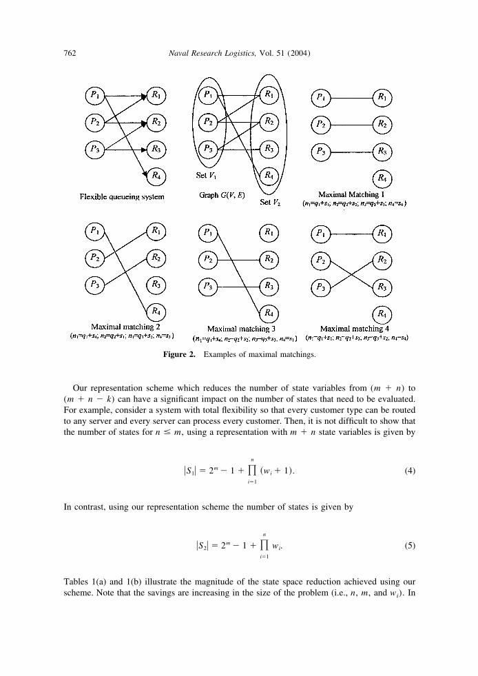
Our representation scheme which reduces the number of state variables from (m n) to(m n k) can have a significant impact on the number of states that need to be evaluated.For example, consider a system with total flexibility so that every customer type can be routedto any server and every server can process every customer. Then, it is not difficult to show thatthe number of states for n � m, using a representation with m n state variables is given by

�S1� � 2m 1 � �i�1

n

�wi � 1�. (4)

In contrast, using our representation scheme the number of states is given by

�S2� � 2m 1 � �i�1

n

wi. (5)

Tables 1(a) and 1(b) illustrate the magnitude of the state space reduction achieved using ourscheme. Note that the savings are increasing in the size of the problem (i.e., n, m, and wi). In

Figure 2. Examples of maximal matchings.


general, the savings are largest when flexibility is reasonably well distributed among servers andcustomers and k is near its maximum value of min(m, n).

3.2. Performance Evaluation

In this section, we develop models for the performance evaluation of flexible queueingsystems. Our approach begins by determining the probability of occurrence of each system statefor the different control policies under consideration. From these probabilities, we show how toobtain various performance measures of interest. We model our system as a continuous timeMarkov chain (CTMC) with state vectors N � (n1, n2, . . . , nq), and ni is as defined insubsection 3.1. Our Markov chain is a birth–death process since the system transitions from itscurrent state through either a single customer arrival or a single customer departure. The limitingprobabilities of system states can be obtained from the balance equations of the Markov chainby equating the rate at which the system enters a state with the rate at which it leaves it. Thisrelationship results in a set of linear equations that can be solved using a general-purpose linearequation solver.

Following the approach in Sheikhzadeh et al., we define for each state vector N � (n1,n2, . . . , nq) two sets of states, type a and type d, depending on whether an arrival or a departurecauses the system to move to state N. We denote these sets of states as Na and Nd, respectively.Elements of Na (Nd) are state vectors Ni

a (Nid), such that ni

a � ni 1 (nid � ni 1) and all

other state variables having the same value as in N. We define �( x) as a function that returns1 if x � 1, and 0 otherwise. We also define

�i � � 1, if 1 � i � n,0, otherwise,

Table 1(a). Percentage reduction in the size of the state space (wi � 4 for i � 1, 2, . . . , n).

n m �S1� �S2� Percentage Difference

3 3 132 71 46.214 4 640 271 57.665 5 3156 1055 66.576 6 15688 4159 73.497 7 78252 16511 78.908 8 390880 65791 83.179 9 1953636 262655 86.56

10 10 9766648 1049599 89.25

Table 1(b). Percentage reduction in the size of the state space (n � m � 6).

wi �S1� �S2� Percentage Difference

2 792 127 83.963 4159 792 80.964 15688 4159 73.495 46719 15688 66.426 117712 46719 60.317 262207 117712 55.118 531504 262207 50.679 1000063 531504 46.85

10 1771624 1000063 43.55


and

i � � 1, if �1 � i � k� or �n � i � m and m k�,0, otherwise.

The variable �i is used to indicate if a state variable ni includes the queue size of a customer i.Similarly, the variable i is used to indicate if a state variable ni includes the state of a serveri. Finally, we define the parameter bi, the upper bound on the state variable ni, as follows:

bi � � wi � 1, if i � �i � 1,wi, if �i � 1 and i � 0,1, otherwise.

Whenever the system is in state N, it is straightforward to show that it leaves this state as aresult of a service completion with rate ¥i�1

q �(ni) i�i and as a result of an arrival with rate¥i�1

q �(bi ni)�i�i. If we use ria (ri

d) to denote the rates at which the system enters state Nfrom Ni

a (Nid), and if we use notation p(N), p(Ni

a) and p(Nid) to denote the steady state

probabilities of those states, we can then write the Markov chain balance equation as follows:

� �i�1

q

��ni� i�i � �i�1

q

��bi ni��i�i�p�N� � �Ni

a�Na

ria p�Ni

a� � �Ni

d�Nd

rid p�Ni

d�, � N � S2.

(6)

The set of linear equations in (6) along with the normalizing equation ¥S2p(N) � 1 forms a set

of �S2� simultaneous equations, which can be solved to determine the steady state probabilities,p(N), N � S2. However, in order to solve for p(N), we need to first define the sets of enteringstates Ni

a and Nid and determine the associated rates ri

a and rid, respectively.

3.2.1. The Sets of Entering States

There are two types of constraints that define whether a state can be included in either set Na

or Nd. The first constraint deals with feasibility. Depending on the routing matrix and the controlpolicies, there are certain states that can never occur. The second restriction stems from therequirement that it should be possible to go from a member of Na (or Nd) to N by a one-steptransition as result of a single arrival or a single departure.

We first consider the set Na. The system can move into state N from Nia, only if ni

a � ni 1 and all other state variables have exactly the same values as in N. That is,

nia � ni 1 and nk

a � nk � k � i. (7)

The state Nia exists only when one of the following mutually exclusive conditions holds:

1 � nia � bi 1 and nl � 0, � l � i, l � Qi, i � �i � 1; (8)

0 � nia � bi 1 and nl � 0, � l � i, l � Qi, i � 0, �i � 1; or (9)


nia � 0 and nr

a � 1, � r � i, r � Ti, i � 1. (10)

Condition 8 states that for nia (ni � qi si since wi � �i � 1) to increase by 1, all the servers

capable of processing customers of type i must be busy. This follows from the fact that we donot allow a queue to form while a feasible server is idle. Note that we do not require that theserver represented by ni be occupied by a customer of type i Condition 9 states that for ni (ni �qi since i � 0) to increase by 1, all the servers capable of processing customer i must be busy.In this case ni can be zero since it represents customer queue size. Condition 10 considers caseswhen ni (ni � qi si or ni � si) increases from 0 to 1. This is possible only if server i is idlewhich occurs only if there are no customers in the queue that can be processed on server i. Fromthe above we can now define set Na as follows:

Na � �Nia : 1 � ni

a � bi 1 and nl � 0, � l � i, l � Qi, i � 1, �i � 1;

0 � nia � bi 1 and nl � 0, � l � i, l � Qi, i � 0, �i � 1; or

nia � 0 and nr

a � 1, � r � i, r � Ti, i � 1; and i � 1, . . . , q�.

Similarly, the system moves into a state N from a state Nid only if ni

d � ni 1 and all otherstate variables maintain the same values as in N. That is,

nid � ni � 1 and nk

d � nk, � k � i. (11)

It is possible to show that the above holds only if one of the following conditions is true:

nid � 1 and nr

d � 1, � r � i, r � Ti, i � 1; (12)

2 � nid � bi and nl

d � 0, � l � i, l � Qi, i � 1, �i � 1; or (13)


d � 0, � l � i, l � Qi, i � 0. (14)

Condition 12 states that a departure would cause nid to decrease from 1 to 0 if there are no other

customers present in queue that can be processed on server i. Condition 13 considers the casewhere ni

d � 2 and follows from the fact that a queue of customer type i cannot form unless allits feasible servers are busy. Condition (14) is similar to (13) when ni describes only the queuesize of a customer type i (ni � qi). Set Nd is thus given by

Nd � �Nid : ni

d � 1 and nrd � 1, � r � i, r � Ti, i � 1;


d � 0, � l � i, l � Qi, i � 1, �i � 1; or


d � 0, � l � i, l � Qi, i � 0, �i � 1; i � 1, . . . , q�.

3.2.2. Transition Rates ria and ri

d

In this section, we show how the transition rates for the control policies we consider can bedetermined. Recall that we define control policies in terms of a server and customer selectionrule combination.


The SP-LQF Policy. Under the SP-LQF policy, servers are selected based on a strict priorityscheme and customers are selected from the class with the longest queue. When either condition(8) or (9) holds, a transition from Ni

a to N clearly occurs with rate

ria � �i. (15)

However, when condition (10) holds, the transition rate depends on the routing priorities. Firstnote that for ni

a to increase from 0 to 1, we need an arrival from a customer type that belongsto the set Ti. Although necessary, this condition is not sufficient since an arrival of a customerof type Pk from the set Ti may not be routed to server i unless server i has the highest priorityamong those available to process customer Pk. This means that the following condition,

�ki � �kj for all j � Qk that satisfy nj � 0 and wj � 1,

must be satisfied. Since the arrival rate of customers of type k is �k, the transition rate ria is given

by

ria � �

k�Ti

�k��ki�,

where

��ki� � � 1, if �ki�1 ��nt�� kt, � k � Ti, � t � Qk; and0, otherwise. (16)

Putting it all together, we have

ria � � ri

a � �i, if 0 � nia � bi 1 and nl � 0, � l � i, l � Qi, �i � 1;�

k�Ti

�k��ki�, if nia � 0 and nr

a � 1, � r � i, r � Ti, i � 1.

Similarly, we can derive the transition rates Nid to N. If condition (12) holds, then we clearly

have rid � �i. When condition (13) or (14) holds, the transition rate depends on the relative size

of the queues. There can be a transition from Nid to N if the queue for customer Pi is one of the

longest queues for any of the servers in the set Qi. In other words, for a server k in the set Qi

to select queue i, queue i must be one of the longest queues in the set Tk (the set of feasiblecustomers for server k). We denote by Bk the number of customers that have the longest queuein the set Tk. When Bk � 1, queue i is selected by server k with probability 1/Bk. Thus, thetransition rate can be written as

rid � �

�i if nid � 1 and nq

d � 1, � q � i, q � Ti, i � 1;

�k�Qi

�k�k�Pi�

Bkif 2 � ni

d � bi, and nld � 0, � l � i, l � Qi, i � 1; and

�k�Qi

�k�k�Pi�

Bkif 1 � ni

d � bi and nld � 0, � l � i, l � Qi, �i � 0,

(17)


where Bk is the number of customer types that have the longest queue in the set Tk, and �k(Pi) �1 if the queue of customer type i is one of the Bk longest queues in the set Tk, and 0 otherwise.

The RR-LQF Policy. The sets of entering states are the same for this queue selection policyas in the SP-LQF control policy. Only the transition rates differ. If an arrival of customer typePk occurs, where Pk is of one of the customer types in set Ti, this arrival has an equal chanceof being routed to any of the idle servers in the set Qk. Thus,

ria � �

ria � �i, if 1 � ni

a � bi 1 and nl � 0, � l � i, l � Qi, i � 1, �i � 1; or0 � ni

a � bi 1 and nl � 0, � l � i, l � Qi, i � 0, �i � 1; and

�k�Ti

�k�k

¥t�Qk�1 ��nt��

, if nia � 0 and nr

a � 1, � r � i, r � Ti, i � 1.(18)

The rate rid is the same as in the SP-LQF case.

The RR-SP Policy. The rate ria for the RR-SP policy is the same as in the RR-LQF policy,

while the rate rid is given as follows. When condition (12) holds, a transition from Ni

d to Nclearly occurs with rate:

rid � �i. (20)

However, when either condition (13) or (14) holds, the transition rate depends on the strictpriority scheme. First note that for ni

d to decrease by 1, we need a departure from a server thatbelongs to the set Qi. Although necessary, this condition is not sufficient since a departure froma server Rk from the set Qi may not decrease ni

d by 1, unless the customer type i has the highestpriority among all the customer types in queue that can be routed to Rk. This means that thefollowing conditions must be satisfied:

�ik � �jk for all j � Tk that satisfy nj � 2 and �j � 1, j � 1 or

�ik � �jk for all j � Tk that satisfy nj � 1 and �j � 1, j � 0.

Since the departure rate from server Rk is �k, the transition rate rid is given by

rid � �

k�Qi

�k��ik�

where

��ik� � � 1, if �ik�1 ��nt 1�� tk, � k � Qi, � t � Tk, vt � t � 1;or �ik�1 ��nt�� tk, � k � Qi, � t � Tk, t � 0; and

0, otherwise.(21)

Putting it all together, we have:


ria � �

�i, if nid � 1 and nr

d � 1, � r � i, r � Ti, i � 1;�k�Qi

�k��ik�, if 2 � nid � bi and nl

d � 0, � l � i, l � Qi, vi � i � 1;

or 1 � nid � bi and nl

d � 0, � l � i, l � Qi, vi � 1, i � 0; and0, otherwise.

(22)

The SP-SP Policy. The rate ria for the SP-SP is the same as in the SP-LQF policy, while the rate

rid is the same as in the RR-SP policy. The transition rates for the remaining policies, namely

SP-RS and RR-RS, can be determined in a similar fashion. The details are omitted for brevity.

3.3. Systems with a Bound on the Total Number of Customers in the System

Our analysis can be extended to system where there is a global, instead of customertype-specific, bound on the number of customers in the system. This means that the maximumnumber of customers that can be allowed in the system (regardless of type) is b. With thisrequirement, it is not difficult to show that a transition from a state Ni

a occurs only if one of thefollowing conditions holds:

nia � 1, �

i�1

q

ni � b, and nl � 0, � l � i, l � Qi, i � 1, �i � 1; (23)

nia � 0, �

i�1

q

ni � b, and nl � 0, � l � i, l � Qi, i � 0, �i � 1; or (24)

nia � 0 and nr

a � 1, � r � i, r � Ti, i � 1. (25)

Similarly, a transition from Nid to N occurs only if one of the following conditions is true:

nid � 1 and nr

d � 1, � r � i, r � Ti, �i � 1; (26)

2 � nid � b and nl

d � 0, � l � i, l � Qi, i � 1; or (27)

1 � nid � b and nl

d � 0, � l � i, l � Qi, i � 0. (28)

The transition rates ria (ri

d) associated with conditions (23)–(25) [(26)–(28)] are the same asthose associated with conditions (8)–(10) [(12)–(14)] of the previous section for each pair ofserver and customer selection rules we consider.

3.4. Performance Measures

From p(N), we can obtain the marginal probability p(ni) associated with the state variable ni.Our primary measure of performance is throughput for each customer type i which can beobtained as follows:


�ip � �i�1 p�ni � bi��, (29)

from which, we can then obtain total system throughput as

�S � �i�1

n

�ip. (30)

We can also derive expressions for throughput due to each server j as

�jR � �j�1 p�nj � 0��. (31)

Several other measures of performance can be obtained as well, including expected queue sizefor each customer type, average utilization of each server, expected total WIP in the system, andexpected flow time.

4. NUMERICAL EXAMPLES AND INSIGHTS

In this section, we use numerical examples to generate some insights into the behavior offlexible queueing systems. We focus on the role flexibility plays and how it interacts with othersystem parameters. We also examine the effect of control policies and examine the interactionsbetween control policies, flexibility and asymmetry in system parameters. The treatment is notmeant to be comprehensive but simply to illustrate how the model can be useful in developingbetter understanding of the behavior of flexible queueing systems. We make five main obser-vations. First, we show that additional flexibility without a well-designed control policy canreduce throughput. Second, for symmetric systems, we show that a chained configuration ofserver/customer flexibilities provides most of the throughput benefits of total flexibility. We alsoshow that increased chaining exhibits diminishing returns. Third, for symmetric systems, weshow that throughput is maximum when flexibility is balanced among the various customers andthe servers. However, we show that this is not necessarily the case for asymmetric systems withheterogeneous servers or asymmetric demand rates. For these systems, we find that chaining isnot always superior to a nonchained configuration. Fourth, we examine the impact of controlpolicies under different conditions of asymmetry. We show that there is a range of asymmetryin which the difference in throughput due to different control policies is maximum. Fifth, weillustrate how strict priorities can be used to model a wide range of policies, including those thattake customer and server flexibility into account. We show that flexibility-based policies canimprove throughput in asymmetric systems with partial flexibility.

OBSERVATION 1: Increasing flexibility for one or more customers can reduce systemthroughput.

Consider the five scenarios shown in Figure 3. The scenarios correspond to systems withvarying customer routing flexibility. Values of system parameters are as follows: �j � 1 for j �1, 2, . . . , 5; �1 � 5.0, �2 � 1.25, �3 � 0.75, �4 � 0.5, �5 � 0.25; and bi � 2 for i �1, . . . , 5. The queue selection rule is SP with the customer with the higher arrival rate assigneda lower priority. Server selection is also of the SP type with servers ordered per the priorityscheme �1 �2 �3 �4 �5 for any customer–server assignment. System throughput


corresponding to each scenario is shown in Table 2(a). In each scenario, we increase theflexibility of one or more customers. As we can see, any increase in flexibility leads to areduction in system throughput. The amount of this decrease is sensitive to whose flexibility,among the customers, is increased. These effects can be explained as follows. In each scenario,greater flexibility is achieved by allowing more customers to be routed to server R1. Thisincreases the overall loading of R1 and increases the probability of balking for all classes thatwere initially assigned to it (e.g., P1). In turn, this leads to lower throughput for these customers,which may not always be matched by increased throughput for customers whose flexibility hasbeen increased. This would be particularly the case when the demand rates for the originalcustomers are high or when the flexibility of the newly assigned customer is already high (seeFigs. 14 and 15 for additional examples). Clearly, using a better control policy could mitigatethese effects. For example, as shown in Table 2(b), using the LQF instead of the SP rule in

Figure 3. Flexibility scenarios for Observation 1.

Table 2(a). The effect of higher flexibility on throughput.

Scenario 1

�1R �2

R �3R �4

R �5R �S

0.967741 0.99253 0.654998 0.468458 0.228868 3.3126�1

p �2p �3

p �4p �5

p �S

0.967742 0.6471 0.698342 0.57678 0.422632 3.3126

Scenario 2

�1R �2

R �3R �4

R �5R �S

0.978557 0.610363 0.67052 0.56896 0.420293 3.24869�1

p �2p �3

p �4p �5

p �S

0.813833 1.0776 0.659329 0.468943 0.228985 3.24869

Scenario 3

�1R �2

R �3R �4

R �5R �S

0.982466 0.613041 0.654076 0.547927 0.414268 3.21178�1

p �2p �3

p �4p �5

p �S

0.749 1.07363 0.689526 0.470339 0.229287 3.21178

Scenario 4

�1R �2

R �3R �4

R �5R �S

0.98429 0.614561 0.655705 0.535872 0.400271 3.1907�1

p �2p �3

p �4p �5

p �S

0.719609 1.07099 0.689018 0.481092 0.229986 3.1907

Scenario 5

�1R �2

R �3R �4

R �5R �S

0.985452 0.615856 0.65734 0.53666 0.373837 3.16914�1

p �2p �3

p �4p �5

p �S

0.691541 1.06837 0.688001 0.481508 0.239724 3.16914


selecting customers tends to dampen the above effects. These effects would altogether disappearif an optimal control policy were used.

Several recent studies (Hopp, Tekin, and van Oyen [17], Jordan and Graves [18], andSheikhzadeh, Benjaafar, and Gupta [25]) have shown in a variety of contexts that a chainedconfiguration in which each customer can be routed to one of two neighboring servers and eachserver can process customers from two neighboring classes achieves most of the benefits of totalflexibility. In the following observation, we confirm that this is true for symmetric systems (i.e.,systems with identical servers, customer classes, and queue sizes). We also show that higherorder chaining exhibits diminishing returns. A system with chaining of order K (K � 2) refersto systems where each customer can be routed to K neighboring servers and each server canprocess K neighboring customers. Systems with varying orders of chaining are shown in Figure 4.

OBSERVATION 2: In a symmetric system, increased chaining exhibits diminishing returnswith most of the value of total flexibility achieved with the initial chain.

To illustrate the above result, consider the system scenarios shown in Figure 4. The scenarioscorrespond to systems with progressively higher orders of chaining. Scenario 1 corresponds toa system with no flexibility and scenario 6 to a system with total flexibility (chaining of orderK � 6). For each scenario, we obtain the corresponding throughput. Representative results areshown in Figure 5 (system parameters for the data we show are: �j � 1 for j � 1, . . . , 6; �i �� and bi � 2 for i � 1, . . . , 6, and the control policy is SP-LQF). As we can see, most of theincrease in throughput is achieved by forming the initial chain. Higher orders of chainingincrease throughput only marginally and in progressively diminishing amounts. These resultssuggest that total flexibility, which corresponds to chaining of maximal order, is generallyunjustified if increases in flexibility require significant investments.

Although increases in chaining exhibit diminishing returns, this is not true with increases inflexibility in general. In Figure 7, we illustrate the effect of gradually increasing flexibility one

Table 2(b). The effect of higher flexibility on throughput (LQF Policy).

Scenario 1

�1R �2

R �3R �4

R �5R �S

0.967742 0.524806 0.721104 0.590107 0.524955 3.32871�1

p �2p �3

p �4p �5

p �S

0.967742 1.02965 0.648367 0.46144 0.221512 3.32872

Scenario 2

�1R �2

R �3R �4

R �5R �S

0.974386 0.503267 0.708753 0.588273 0.524766 3.29945�1

p �2p �3

p �4p �5

p �S

0.88841 1.07656 0.651316 0.46162 0.221533 3.29944

Scenario 3

�1R �2

R �3R �4

R �5R �S

0.972746 0.518508 0.710992 0.575389 0.523418 3.30105�1

p �2p �3

p �4p �5

p �S

0.908242 1.03606 0.67215 0.462915 0.221684 3.30105

Scenario 4

�1R �2

R �3R �4

R �5R �S

0.970527 0.523728 0.719368 0.581548 0.514851 3.31002�1

p �2p �3

p �4p �5

p �S

0.934724 1.03055 0.650816 0.471252 0.222678 3.31002

Scenario 5

�1R �2

R �3R �4

R �5R �S

0.970812 0.524269 0.720242 0.585485 0.502968 3.30378�1

p �2p �3

p �4p �5

p �S

0.928066 1.03008 0.649418 0.464136 0.232079 3.30378


customer at a time (i.e., adding a single arc at a time to the graph). In this case, each level ofchaining is attained via a series of increases to the number of arcs (see Fig. 6). From Figure 7,we see that, surprisingly, the marginal increase in throughput is not always decreasing in thenumber of arcs. In fact, within each level of chaining, it exhibits increasing returns, with the lastlink in each chain realizing the largest marginal gain in throughput. This result furtherunderscores the importance of forming fully connected chains. This is different from theobservation made in Hopp, Tekin, and van Oyen [17] for serial systems, where only the last linkin the chain is found to exhibit increasing returns.

Figure 4. Flexibility scenarios for Observation 2.

Figure 5. The effect of chaining on system throughput.


OBSERVATION 3: In a symmetric system, a balanced allocation of flexibility among thecustomers leads to higher throughput.

Consider the four system scenarios shown in Figure 8. The scenarios correspond to systemswhere the total amount of customer flexibility (i.e., the number of edges connecting customersto servers) remains fixed but the allocation of this flexibility (edges) is varied. System through-put for varying levels of flexibility asymmetry is shown in Figure 9 (values of system parameters

Figure 6. Increasing flexibility one arc at a time.

Figure 7. The effect of flexibility on system throughput.


here and in subsequent observations, unless noted, are the same as in Observation 2; the resultsare shown for the SP-LQF policy with similar effects observed for other policies), from whichit is clear that increased balancing in customer flexibility leads to higher throughput.

A balanced allocation is however not always optimal. In fact, as we note in the followingobservation, an asymmetric allocation of flexibility can be more beneficial when there isasymmetry in customer demand rates.

Figure 8. Flexibility allocation scenarios for Observation 3.

Figure 9. The effect of flexibility asymmetry on system throughput.


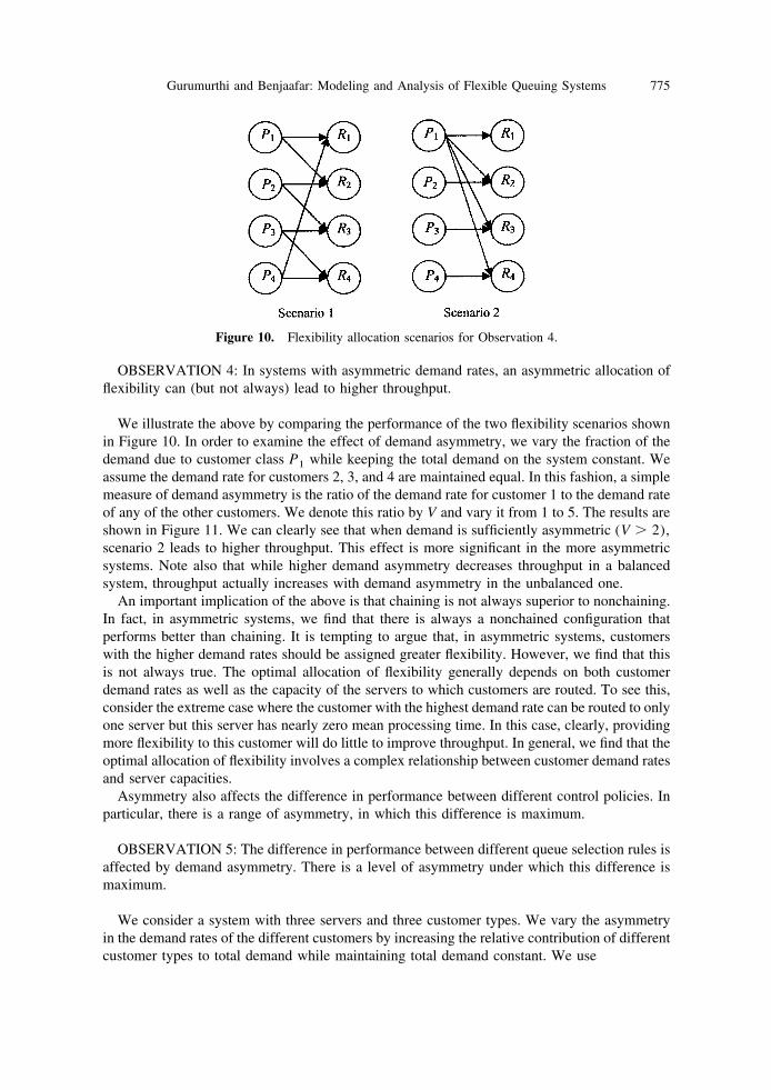
OBSERVATION 4: In systems with asymmetric demand rates, an asymmetric allocation offlexibility can (but not always) lead to higher throughput.

We illustrate the above by comparing the performance of the two flexibility scenarios shownin Figure 10. In order to examine the effect of demand asymmetry, we vary the fraction of thedemand due to customer class P1 while keeping the total demand on the system constant. Weassume the demand rate for customers 2, 3, and 4 are maintained equal. In this fashion, a simplemeasure of demand asymmetry is the ratio of the demand rate for customer 1 to the demand rateof any of the other customers. We denote this ratio by V and vary it from 1 to 5. The results areshown in Figure 11. We can clearly see that when demand is sufficiently asymmetric (V � 2),scenario 2 leads to higher throughput. This effect is more significant in the more asymmetricsystems. Note also that while higher demand asymmetry decreases throughput in a balancedsystem, throughput actually increases with demand asymmetry in the unbalanced one.

An important implication of the above is that chaining is not always superior to nonchaining.In fact, in asymmetric systems, we find that there is always a nonchained configuration thatperforms better than chaining. It is tempting to argue that, in asymmetric systems, customerswith the higher demand rates should be assigned greater flexibility. However, we find that thisis not always true. The optimal allocation of flexibility generally depends on both customerdemand rates as well as the capacity of the servers to which customers are routed. To see this,consider the extreme case where the customer with the highest demand rate can be routed to onlyone server but this server has nearly zero mean processing time. In this case, clearly, providingmore flexibility to this customer will do little to improve throughput. In general, we find that theoptimal allocation of flexibility involves a complex relationship between customer demand ratesand server capacities.

Asymmetry also affects the difference in performance between different control policies. Inparticular, there is a range of asymmetry, in which this difference is maximum.

OBSERVATION 5: The difference in performance between different queue selection rules isaffected by demand asymmetry. There is a level of asymmetry under which this difference ismaximum.

We consider a system with three servers and three customer types. We vary the asymmetryin the demand rates of the different customers by increasing the relative contribution of differentcustomer types to total demand while maintaining total demand constant. We use

Figure 10. Flexibility allocation scenarios for Observation 4.


V ��1

�2�

�2

�3

as our measure of demand asymmetry. We compare two customer selection rules, SP1 and SP2.Under policy SP1, we give highest priority to the customer class with the lowest demand rate(class 3). Under SP2, we give highest priority to the customer class with the highest demand rate(class 1). The difference in throughput between the two rules is shown in Figure 12 (the resultsare shown for �i � � � 1 for i � 1, . . . , 3; the notation � � (�1 �2 �3)/3 is used todenote overall system loading). As we can see, the difference is maximum when asymmetry isin the mid-range.

A similar effect is observed with respect to server selection rules and asymmetries inprocessing rate. In that case, we find that the impact of server selection rules is insignificantwhere processing rate asymmetry is either very high or very low. It is however, significant whenthe asymmetry is in the mid-range.

OBSERVATION 6: In asymmetric systems, control policies that take advantage of customerand server flexibility, as well as the available capacity to these customers and the customersdemand rates, can lead to higher throughput.

We compare the following four policies. Under the first policy, policy H1, servers andcustomer classes are assigned priorities based on their flexibility. The server with the least

Figure 11. The effect of demand asymmetry.


flexibility is assigned highest priority and the same for customers. Flexibility is measured by thenumber of customers a server can process or the number of servers to which a customer can beassigned. Under the second policy, policy H2, servers are assigned priorities based on the ratioof the sum of arrival rates of all customers that can be assigned to a server to the server’sprocessing rate. That is, each server j ( j � 1, . . . , m) is assigned a priority based on the ratio¥i�1

n aij�i/�j with lower ratios corresponding to higher priorities. Similarly, customers areassigned priorities based on the ratio of a customer’s arrival rate to the sum of the processingrates of servers to which the customer can be assigned. That is, each customer i (i � 1, . . . ,n) is assigned a priority based on the ratio �i/¥j�1

m aij�j, with higher ratios corresponding tohigher priorities. Hence, policy H2 gives priority to servers with the least potential load and tocustomers with the least potential available capacity. Under the third policy, policy H3, servers(customers) are assigned priorities based on their service (arrival) rates with higher ratescorresponding to higher priorities. The fourth policy, H4, is included for benchmarking andcorresponds to the RR-RS policy.

We consider a system with five customer classes and five servers. We consider 21 flexibilityconfiguration scenarios. We start with a dedicated scenario in which each customer can berouted to only one server and each server can process only one customer (scenario 1). Inscenarios 2–6, we increase flexibility by adding one link at a time between customers andservers until we reach a chained configuration (i.e., in scenario 2 customer 1 can be assigned toservers 1 or 2, in scenario 3, customer 1 can be assigned to servers 1 or 2 and customer 2 canbe assigned to servers 2 or 3, etc.). In scenarios 7–21, we further increase the flexibility onecustomer at a time and one link at a time starting with customer 1 until each customer has fullflexibility (e.g., in scenario 7, customer 1 can be assigned to either servers 1, 2, or 3, in scenario

Figure 12. The effect of demand on performance of queue selection policies.


8, it can be assigned to either servers 1, 2, 3, or 4, etc.). Scenario 21 corresponds to a systemwith full flexibility where any customer can be routed to any server and any server can processany customer.

We consider five levels of system loading, L1 � 0.6, L2 � 0.9, L3 � 1.2, L4 � 1.5, andL5 � 1.8, where Li � ¥i�1

n �i/¥j�1m �j for i � 1, . . . , 5. We also consider four levels of

demand and service rate asymmetry, A1, A2, A3, and A4. For asymmetry level A1, �1 � 0.1and �j � �j1 0.45 for j � 2, . . . , 5, and �5 � 0.1 � L1, and �i � �i1 0.45 �Li for i � 2, . . . , 5. For asymmetry level A2, we assign equal processing rates and servicesrates to all the customers and all the servers. For level A3, we invert the assignments in level A1,by setting �5 � 0.1 and �j � �j1 0.45; j � 1, . . . , 4, and by letting �1 � 0.1 � L1;�i � �i1 0.45 � Li for i � 2, . . . , 5. For level A4, the demand rates are the same as inA1 and the service rates are the same as in A3.

The effect of the different control policies for the different flexibility configurations andasymmetry levels is illustrated in Figures 13–15 (the results are shown for systems with bufferlevels bi � 3 for i � 1, . . . , 5, but are qualitatively similar for other buffer values). As we cansee, from Figures 13 and 14, policy H2 dominates the other policies, suggesting that an optimalpolicy would take into account both the flexibility of servers and customers as well as thecapacity available to the customers relative to their demand rates. The results also suggest thatwhen there are significant asymmetries in demand and service rates, assigning priorities basedon these rates could be more helpful than assigning priorities based on flexibility (see Fig. 13).Figure 14 illustrates how higher flexibility under a suboptimal policy, such as H3 or H4, couldlead to lower throughput (this effect is observed even when there is symmetry in demand andservice rates).

Figure 13. The joint effect of control policies and flexibility (scenario A1-L5).


Figure 14. The joint effect of control policies and flexibility (scenario A4-L5).

Figure 15. The effect of flexibility on the percentage difference in throughput between systems A1 andA3 (policy H2).


Figures 13 and 14 illustrate how the effect of increasing flexibility could be differentdepending on the asymmetry in demand and service rates. In particular, flexibility is mostvaluable when it is associated with either the fastest servers or the customers with the largestdemand (this explains the observed large jumps in throughput with one step increases inflexibility). More importantly, the results show that although there is value to choosing a goodcontrol policy, the effect of control policies is less significant than that of flexibility. An increasein flexibility, if it is carefully designed, can lead to significantly larger improvements inthroughput than can be achieved by improving control alone.

Finally, we note that the effect of flexibility can vary widely depending on the asymmetry indemand and service rates. For the same number of links between customers and servers (and forthe same aggregate capacity and demand), throughput can vary widely depending on howcapacity (demand rates) is distributed among the servers (customers). This is dramaticallyillustrated in Figure 15 where the percentage difference in throughput between systems withasymmetry A1 and systems with asymmetry A3 is shown for different levels of flexibility anddifferent levels of loading. Note that an increase in flexibility can switch the ordering of the twosystems in either direction, so that an increase in flexibility can make a particular distributionof capacity and demand rates more or less desirable. This points to the need to carry out,whenever possible, capacity allocation jointly with flexibility design.

6. CONCLUDING COMMENTS

In this paper, we presented a framework for the representation, modeling and analysis offlexible queueing systems. The analytical model allows for the analysis of general systemconfigurations with an arbitrary number of customers and servers, an arbitrary flexibility matrix,asymmetric demand and processing rates, asymmetric bounds on customer queue sizes, and awide range of control policies. The models are generic and can be used to analyze flexiblequeueing systems in a variety of applications. They can also serve as a decision support tool forthe planning and design of these systems. Furthermore, our characterization of the probabilitydistribution of system states and the transition probability between these states offers theopportunity to formulate optimal control problems (e.g., using the framework of a Markovdecision process).

Our model can be extended in a variety of ways. This includes relaxing the assumptions ofPoisson demand and exponential processing times and allowing service times to vary bycustomer and server. It would then be useful to examine the impact of demand and servicevariability on different system configurations and different control policies. In many applica-tions, such as manufacturing, the processing of multiple customers on the same servers isaccompanied by losses in efficiencies due to switchover times or costs. It would be worthwhileto extend the models to account for these inefficiencies. In other applications, such as telecom-munication networks, the processing of a customer requires the simultaneous contribution ofmore than one server. For these applications, there is a need to extend the analysis to systemswhere customers consume varying amounts of capacity.

ACKNOWLEDGMENTS

The authors are grateful to William Cooper and Mike Taaffe for many useful comments onan earlier draft. The research of the second author is supported by NSF through GrantsDMII-9908437 and 9988721. We are also grateful to an anonymous reviewer for many helpfulcomments.


REFERENCES

[1] R.K. Ahuja, T.L. Magnanti, and J.B. Orlin, Networks flows, Prentice Hall, Englewood Cliffs, NJ,1993.

[2] O.Z. Aksin and F. Karaesmen, Designing flexibility: Characterizing the value of cross-trainingpractices, Working Paper, INSEAD, Cedex, France, 2002, www.ku.edu.tr/�fkaraesmen/pdfs/flex2102.pdf.

[3] M. Armony, Queueing networks with interacting service resources, Ph.D. thesis, Stanford University,Stanford, CA, 1999.

[4] S. Benjaafar, Performance bounds for the effectiveness of pooling in multi-processing systems,European J Oper Res 87 (1995), 375–388.

[5] S. Benjaafar, Demand allocation in multi-product/multi-facility make-to-stock systems, ManagementSci (2004), in review.

[6] S. Benjaafar and D. Gupta, Workload allocation in multi-product/multi-facility production systemswith setup times, IIE Trans 31 (1998), 339–352.

[7] J.A. Buzacott, Commonalities in reengineered business processes: Models and issues, ManagementSci 42 (1996), 768–782.

[8] J.A. Buzacott and J.G. Shanthikumar, Stochastic models of manufacturing systems, Prentice Hall,Englewood Cliffs, NJ, 1993.

[9] J.M. Calabrese, Optimal workload allocation in open networks of multi-server queues, ManagementSci 38 (1992), 1792–1802.

[10] R. Cooper, Introduction to queueing theory, 2/E, North-Holland, Amsterdam, 1981.[11] S. Even and R.E. Tarjan, Network flow and testing graph connectivity, SIAM J Comput 4 (1975),

507–518.[12] N. Gans, G. Koole, and A. Mandelbaum, Telephone call centers: Tutorial, review and research

prospects, Manufacturing Serv Oper Management 5 (2003), 79–141.[13] O. Garnett and A. Mandelbaum, An introduction to skills routing and its operational complexities,

Teaching Note, Technion, Haifa, Israel, 2001, www.ie.technion.ac.il/serveng/Homeworks/HW9.pdf.[14] B. Hajek, Optimal control of two interacting service stations, IEEE Trans Automat Control AC-29

(1984).[15] R.W. Hall, Queueing methods: For services and manufacturing, Prentice Hall, Englewood Cliffs, NJ,

1991.[16] J.M. Harrisson and M.J. Lopez, Heavy traffic resource pooling in parallel server systems, Queueing

Syst 33 (1999), 339–368.[17] W. Hopp, E. Tekin, and M.P. Van Oyen, Benefits of skill chaining in production lines with

cross-trained workers, Working Paper, Department of Industrial Engineering and ManagementSciences, Northwestern University, Evanston, IL, 2001.

[18] W.J. Jordan and S.C. Graves, Principles on the benefits of manufacturing process flexibility,Management Sci 41 (1995), 577–594.

[19] L. Kleinrock, Queueing systems: Computer applications, Wiley, New York, 1976, Vol. 2.[20] G. Koole and A. Mandelbaum, Queuing models of call centers, an introduction, Ann Oper Res 113

(2002), 41–59.[21] C.N. Laws, Resource pooling in queueing networks with dynamic routing, Adv Appl Probab 24

(1992), 699–726.[22] A. Mandelbaum and M. Reiman, On pooling in queueing networks, Management Sci 44 (1998),

971–981.[23] K.W. Ross, Multiservice loss models for broadband telecommunication networks, Springer-Verlag,

London, 1995.[24] L.I. Sennot, Stochastic Dynamic Programming and the Control of Queueing Systems, Wiley, New

York, 1999.[25] M. Sheikhzadeh, S. Benjaafar, and D. Gupta, Machine sharing in manufacturing systems: flexibility

versus chaining, Int J Flexible Manuf Syst 10 (1998), 351–378.[26] R.A. Shumsky, Approximation and analysis of a call center with flexible and specialized servers,

Working Paper, University of Rochester, Rochester, 2003, http://omg.simon.rochester.edu/omg-HOME/shumsky/flex_serv.PDF.

[27] D.R. Smith and W. Whitt, Resource sharing for efficiency in traffic systems, Bell Syst Tech J 60(1981), 39–55.


[28] K. Stecke and J.J. Solberg, The optimality of unbalancing both workloads and machine group sizesin closed queueing networks of multiserver queues, Oper Res 45 (1985), 882–910.

[29] S. Stidham, Jr. and R. Weber, A survey of Markov decision models for control of networks of queues,Queueing Syst 13 (1993), 291–314.

[30] Y.T. Wang and R.J.T. Morris, Load sharing in distributed systems, IEEE Trans Comput C-34 (1985),204–217.

[31] W. Winston, Optimality of shortest line discipline, J Appl Probab 14 (1977), 181–189.[32] R. Weber, On the optimal assignment of customers to parallel queues, J Appl Probab 15 (1978),

406–413.[33] W. Whitt, Stochastic models for the design and management of customer contact centers: Some

research directions, Working Paper, Columbia University, New York, 2002, www.columbia.edu/�ww2040/IEOR6707F02.html.


Documents

Modeling and Analysis of Flexible Queueing Systems · Modeling and Analysis of Flexible Queueing Systems ... uniﬁed framework for the modeling and analysis of these systems under