Embed Size (px)
Citation preview

Graduate Theses, Dissertations, and Problem Reports
2014
Modeling and Analysis of Distribution System with Demand Modeling and Analysis of Distribution System with Demand
Response and Electric Vehicles in Personal and Public Response and Electric Vehicles in Personal and Public
Transportation Transportation
Venkata Satish Kasani West Virginia University
Follow this and additional works at: https://researchrepository.wvu.edu/etd
Recommended Citation Recommended Citation Kasani, Venkata Satish, "Modeling and Analysis of Distribution System with Demand Response and Electric Vehicles in Personal and Public Transportation" (2014). Graduate Theses, Dissertations, and Problem Reports. 370. https://researchrepository.wvu.edu/etd/370
This Thesis is protected by copyright and/or related rights. It has been brought to you by the The Research Repository @ WVU with permission from the rights-holder(s). You are free to use this Thesis in any way that is permitted by the copyright and related rights legislation that applies to your use. For other uses you must obtain permission from the rights-holder(s) directly, unless additional rights are indicated by a Creative Commons license in the record and/ or on the work itself. This Thesis has been accepted for inclusion in WVU Graduate Theses, Dissertations, and Problem Reports collection by an authorized administrator of The Research Repository @ WVU. For more information, please contact [email protected].

Modeling and Analysis of Distribution System with Demand
Response and Electric Vehicles in Personal and Public
Transportation
By
Venkata Satish Kasani
Thesis submitted to the
Benjamin M. Statler College of Engineering and Mineral Resources
at West Virginia University
in partial fulfillment of the requirements for the degree of
Master of Science
in
Electrical Engineering
Dr. Sarika Khushalani Solanki, Ph.D., Chair
Dr. Jignesh Solanki, Ph.D.
Prof. Muhammed A. Choudhry, Ph.D.
Lane Department of Computer Science and Electrical Engineering
Morgantown, West Virginia
2014
Keywords: Plug-in Hybrid Electric Vehicles (PHEVs), Personal Rapid Transit
(PRT), Battery Electric Vehicles (BEVs), OpenDSS, Demand Response, Three
Phase Unbalanced Distribution power flow.
Copyright 2014 Venkata Satish Kasani
ABSTRACT
Modeling and Analysis of Distribution System with Demand Response and Electric
Vehicles in Personal and Public Transportation
Venkata Satish Kasani
Master of Science in Electrical Engineering
West Virginia University
Advisor: Dr. Sarika Khushalani Solanki, Ph.D.
The government policies and cost benefits led to the surge in penetration of Plug-in Hybrid
Electric Vehicles (PHEVs) and Battery Electric Vehicles (BEVs) into both public and private sectors,
challenging the electric grid’s potential to maintain its stability and efficiently serve the purpose. The
penetration of PHEVs brings technological advancements and environmental benefits to the traditional
transportation and electrical power systems. Designing of appropriate charging methods to satisfy PHEV
owners helps to improve system performance and avoid transmission and distribution system expansion.
The primary objective of this thesis is to model a coordinated charging algorithm to charge
maximum number of PHEVs with the existing infrastructure at a Charging Station (CS) located in
residential locality. The stochastic driving patterns of PHEVs are studied and different charging strategies
are developed. The Optimized charging scheme is obtained for American Electric Power utility
distribution feeder modeled in OpenDSS. Further, PHEV customers are modeled into price responsive
consumers capable of participating in Demand Response programs to economically charge their vehicles
and render support to the stabilization of power system. Consumer behavior modeling has been done by
developing extensive demand-price elasticity matrices (PEMs) which are utilized to calculate the level of
demand response.
This thesis also proposes a concept of converting the existing Personal Rapid Transit (PRT)
system from guideway power rail propelling vehicles to Battery Electric Vehicles (BEVs) by developing
a novel routing algorithm based on the data provided by West Virginia University’s Department of
Transportation and Parking. This turns into a feasibility analysis of implementing new EV technologies in
electrification of public transportation. The routing algorithm involves Mixed Integer Linear
Programming (MILP) Optimization resulting in hourly schedule of all the vehicles satisfying the
passenger demand. The effect of charging load of BEVs on the electrical distribution system is analyzed
by performing a time series simulation on AEP distribution feeder.
Additionally, the impact of PHEV charging on power market prices i.e. Locational Marginal Prices
(LMP) in a distribution microgid scenario is presented. Locational marginal pricing is a market based
wholesale pricing approach adopted by six out of ten national electricity markets. The uncoordinated
charging of EVs results in unplanned peak demand causing system changes and fluctuation of LMP. The
stabilizing effect of coordinated charging scheme is demonstrated on IEEE 13 Node test system.

iii
ACKNOWLEDGEMENTS
I would like to express my sincere gratitude to my advisor, Dr. Sarika Khushalani Solanki, for
her invaluable guidance, support, and encouragement. I thank Dr. Sarika for believing in me that I can
accomplish this goal with hard work and sincere effort. I thank her for providing me that confidence
which lead to completion of this research work. Next, I would like to thank my second committee
member Dr. Jignesh Solanki. It was from him that I learned the difference between mere hard work and
hard work with focus and dedication. Both Dr. Sarika Khushalani Solanki and Dr. Jignesh Solanki have
been with me, guiding me throughout my two years of research. I would also like to thank my other
committee member Dr. Muhammed A. Choudhry, whose feedback and reviews helped me improve
the quality of this thesis.
I gratefully acknowledge the financial support provided through Graduate Teaching
Assistantship by Freshman Engineering Department, West Virginia University. Special thanks to Dr.
Robin Hensel and Michelle Poland for their constant support.
I would like to thank my parents for their moral support throughout my graduate studies. Their
love and affection have helped me overcome the toughest of challenges during these two hard years.
Lastly, but in no sense the least, I am thankful to all my friends who made my stay at the West Virginia
University a memorable and valuable experience.

iv
Contents
ABSTRACT ................................................................................................................................................... i
List of Figures ............................................................................................................................................. vii
List of Tables ............................................................................................................................................. viii
Chapter 1: Introduction ........................................................................................................................... 1
1.1. Background ................................................................................................................................... 1
1.2 Electric Vehicles – Definition and Types ..................................................................................... 2
1.2.1 Battery Electric Vehicles ...................................................................................................... 2
1.2.2 Plug-in Hybrid Electric Vehicle ............................................................................................ 3
1.3 Charging of EVs ........................................................................................................................... 3
1.4 PHEVs – Benefits and Challenges ................................................................................................ 3
1.4.1 Benefits ................................................................................................................................. 3
1.4.2 Challenges ............................................................................................................................. 4
1.5 Demand Response ......................................................................................................................... 5
1.6 Locational Marginal Prices ........................................................................................................... 6
1.7 Electrification of Public Transportation ........................................................................................ 7
1.8 Problem Statement ........................................................................................................................ 8
1.9 Approach ....................................................................................................................................... 8
1.9.1 Coordinated Charging Strategy ............................................................................................. 9
1.9.2 PRT Routing Algorithm ........................................................................................................ 9
1.9.3 PHEV Charging Effects on Market Prices .......................................................................... 10
1.10 Outline......................................................................................................................................... 10
Chapter 2: LITERATURE REVIEW ................................................................................................... 11
2.1 PHEV Operating Principle .......................................................................................................... 11
2.2 Charging Methods – Types ......................................................................................................... 11
2.3 Evolution of Charging Strategies ................................................................................................ 12
2.4 Practical Demonstration of PHEV Charging Stations ................................................................ 13

v
2.4.1 San Diego’s Fashion Valley Mall Charging Station, CA.................................................... 13
2.4.2 Trans-Canada Highway Charging Station, Canada ............................................................ 13
2.4.3 Chargepoint, U.S ................................................................................................................. 14
2.5 PHEV Customer Behavior Modeling ......................................................................................... 14
2.6 Demand Response – History and Evolution ............................................................................... 15
2.7 Demand Response and Consumer Behavior Modeling .............................................................. 15
2.8 Personal Rapid Transit System ................................................................................................... 16
2.8.2 Power System Details ......................................................................................................... 17
2.9 Market Prices .............................................................................................................................. 18
2.9.1 Market Clearing Price ......................................................................................................... 18
2.9.2 Locational Marginal Prices ................................................................................................. 18
Chapter 3: MATHEMATICAL MODEL AND FORMULATION ..................................................... 19
3.1 Vehicular Behavior: Extraction of Probability Distribution Functions ...................................... 19
3.2 Modeling of Demand Response .................................................................................................. 21
3.2.1 Price Elasticity Matrix – Fundamentals .............................................................................. 21
3.2.2 Customer Rationality Assumptions..................................................................................... 22
3.3 Coordinated Charging Strategy ................................................................................................... 25
3.4 LMP and OPF Model .................................................................................................................. 26
3.5 PRT Routing Algorithm .............................................................................................................. 28
Chapter 4: SIMULATION TOOLS AND SOFTWARE ...................................................................... 32
4.1 Open Distribution System Simulator (OpenDSS) ....................................................................... 32
4.1.1 Extensive Range of Solution Modes ................................................................................... 34
4.1.2 COM Interface .................................................................................................................... 35
4.2 MATLAB .................................................................................................................................... 36
4.2.1 MATLAB Optimization Toolbox ....................................................................................... 36
4.3 IBM ILOG CPLEX Optimizer .................................................................................................... 36
Chapter 5: SIMULATION AND RESULTS ........................................................................................ 38

vi
5.1 Distribution Power Flow Results for Feeder 2 of AEP System .................................................. 38
5.2 PHEV Integration Study on Utility Distribution Feeder ............................................................. 39
5.2.1 Specifications of PHEV Charging Station .......................................................................... 40
5.2.2 Uncoordinated Charging and Monte Carlo Simulation....................................................... 40
5.2.3 Coordinated Charging of PHEVs ........................................................................................ 42
5.2.4 Voltage Profile of the Feeders ............................................................................................ 43
5.2.5 Load Profiles of Distribution Transformers ........................................................................ 46
5.2.6 Comparison between Scenarios 3 and 4 .............................................................................. 47
5.2.7 Demand Response Application ........................................................................................... 48
5.3 PRT Distribution System Analysis ............................................................................................. 49
5.4 PHEV Impacts on LMPs ............................................................................................................. 54
Chapter 6: CONCLUSION AND FUTURE WORK ............................................................................ 58
6.1 Conclusion .................................................................................................................................. 58
6.1.1 Coordinated Charging Method ............................................................................................ 58
6.1.2 PRT Routing Algorithm ...................................................................................................... 58
6.2 Future Work ................................................................................................................................ 59
References ................................................................................................................................................... 60

vii
List of Figures
Figure 2-1 Aerial view – PRT system of WVU, Morgantown ................................................................... 17
Figure 3-1 PDFs of (a) Distance Travelled and (b) Home Arrival Time .................................................... 20
Figure 3-2Distance and Time between possible set of station pairs ........................................................... 30
Figure 4-1 OpenDSS Configuration ........................................................................................................... 33
Figure 4-2 OpenDSS Standalone EXE User Interface ................................................................................ 34
Figure 4-3 Solution Modes in OpenDSS .................................................................................................... 35
Figure 4-4 Path setting for CPLEX for MATLAB ..................................................................................... 37
Figure 5-1 OpenDSS power flow plot for Feeder 2 .................................................................................... 38
Figure 5-2 AEP Feeder model with PHEV Charging Stations and meter locations ................................... 40
Figure 5-3 MCS plot of State-of-Charge .................................................................................................... 41
Figure 5-4 MCS plot of Hourly Charging Demand .................................................................................... 41
Figure 5-5 Voltage profile for 24-hours of Feeder 2................................................................................... 43
Figure 5-6 Transformer loading for different charging methods ................................................................ 43
Figure 5-7 Feeder 2 Voltage Profile - Base Case ........................................................................................ 44
Figure 5-8 Feeder 2 Voltage Profile - Uncoordinated Charging ................................................................. 45
Figure 5-9 Feeder 2 Voltage Profile - Coordinated Charging ..................................................................... 45
Figure 5-10 Distribution Transformer Loading Patterns ............................................................................ 46
Figure 5-11 Time taken by random vehicles to reach 70% SOC ................................................................ 47
Figure 5-12 Battery capacities of late arrival vehicles ................................................................................ 48
Figure 5-13 Transformer loading for different charging methods - with Demand Response ..................... 49
Figure 5-14 Hourly passenger demand at all 5 stations .............................................................................. 50
Figure 5-15 Number of vehicles at each station pair .................................................................................. 50
Figure 5-16 AEP Feeder-2 with PRT Stations ............................................................................................ 51
Figure 5-17 Total number of BEVs in Service and Charging modes ......................................................... 52
Figure 5-18 Base load and charging load of AEP distribution feeder ........................................................ 52
Figure 5-19 Voltage profile for 24-hours at all metered locations .............................................................. 53
Figure 5-20 Voltage profile of Case-1 and 2 .............................................................................................. 53
Figure 5-21 IEEE 13 Node Test Feeder ...................................................................................................... 54
Figure 5-22: 24-hour multiplier for load nodes........................................................................................... 56
Figure 5-23: LMPs at Different Nodes ....................................................................................................... 56
Figure 5-24: PHEV Charging Effects on LMP…………….……………………………………………...57

viii
List of Tables
Table 3-1. Hourly Day Ahead RTP with Self Elasticity Coefficients ........................................................ 23
Table 3-2. A Section of PHEV Consumer’s PEM ...................................................................................... 24
Table 5-1: Summary of Power flow for Feeder 2 ....................................................................................... 38
Table 5-2. PHEV Penetration and Loading in the Test Feeder ................................................................... 42
Table 5-3: Transformer Loading Analysis .................................................................................................. 46
Table 5-4: Generator Data .......................................................................................................................... 55
Table 5-5: Load Data .................................................................................................................................. 55

1
Chapter 1: Introduction
1.1. Background
The electric power system is one of the highly invested industries undergoing constant
technology renovations in all the three fields - generation, transmission and distribution; emerging into
more complex grid to efficiently serve its purpose. The resultant of these innovations leads to SCADA
Management, Smart Grid, Distribution Operations and Automation in Electric industry. Energy
deregulation has drastically changed the industry backdrop over the last decade generating new business
models and turning others upside down.
The SCADA and EMS is the brain and central nervous system of utility operations which enables
the success of current initiatives including Smart Grid deployment and Distributed Generation. Smart
Grid is a podium for converting electric utility business models from customer enablement and improved
operations to new ways to accomplish supply and demand. Some of the features of today’s Smart Grids as
described in [1] are as follows –
1. Distribution Automation (DA): System monitoring and automation, integrated Volt-VAR
control, communication infrastructure and operating efficiency are common distribution utility
goals that present challenges due to the nature of distribution systems.
2. Automated Metering Infrastructure (AMI): AMI is the foundation technology of Smart Grid
used by the utilities for enabling monitoring of feeders and transformers, outage management,
fault detection, distributed generation and EV integration.
3. Geographic Information Systems (GIS): Improving operating efficiency, system reliability and
safety to manage system assets and electrical network connectivity is the main goal of GIS. The
smart grid features of DA, AMI depend on the accurate asset records and locational data
managed in GIS
4. Demand Management System (DMS): Managing demand has become more and more important
for power delivery utilities. Increased penetration of non-dispatchable renewables and
unpredicted loads such as EVs have increased intermittencies associated with development of
new generation resources, making demand response a critical component of smart grid
implementation.

2
1.2 Electric Vehicles – Definition and Types
Though the political motive of reducing dependency on foreign oil initiated the revolution of
Plug-in Hybrid Electric Vehicles (PHEVs) and Battery Electric Vehicles (BEVs), the characteristics like
low greenhouse gas emissions and related economies are the driving factors behind their popularity. The
Federal government has designed policies aiming at 1 million PHEVs on road by 2015 [2] by providing
incentives and tax exemptions. A significant contribution to pollutants due to Internal Combustion Engine
(ICE) vehicles led to electrification of public transportation by introduction of BEVs and power train
vehicles. Stabilizing the power system encompassing PHEVs and BEVs is a challenging issue in the near
future as charging the vehicles imparts an additional electrical load on the system. Satisfying the PHEV
owners with flexible charging schedules and maximizing social benefit by maintaining the system within
network limits is the point of interest. Much emphasis is laid on facilitating the increasing load due to EV
charging by maximum utilization of existing infrastructure with zero or little new reinforcement to the
grid. The near term forecast of penetration of EVs into market is discussed in [3].
Electric vehicles or EVs can be classified into a broad category that comprises any vehicle with a
battery that can be charged by plugging into an electric wall outlet. The first electric vehicle is dated back
to initial decades of 1900, but due to the availability of cheaper fossil fuels – diesel and petrol, the EVs
are dominated by Internal Combustion Engine (ICE) vehicles. Once again in the year 1966, the U.S
introduced a legislation recommending EVs as a means of reducing air pollution. With this initiative, the
market share of EVs plunged to new peaks every year starting from early 21st century [4].
1.2.1 Battery Electric Vehicles
Battery Electric Vehicles (BEVs) are EVs that operate solely on the battery power without any
ICE cycles. A typical BEV consists of a battery and an electric drivetrain and has zero direct emissions.
The introduction of new battery technology, particularly the advancement of Lithium-Ion batteries, has
greatly affected the sales of BEVs in today’s automotive marketplace. In today’s automobile market
Nissan Leaf, Mitsubishi iMiEV, Ford Focus, Tesla Roadster and Chevy Spark fall into the category of
BEVs. BEVs consist of fewer moving parts than an ICE vehicle and the conversion of electricity to
mechanical work by an electric motor is far superior. Therefore the total vehicle efficiency is nearly three
times higher than an ICE vehicle [5]. Different types of batteries available or under development for EV
technology are – Lead/acid, Nickel Metal Hydride, Lithium-Ion (Tesla Roadster, Mitsubishi iMiEV),
Metal Air and Sodium Nickel Chloride or Zebra battery (Think City EV). The battery capacity dictates
the mileage of the vehicle and the charging technology plays a major role in penetration of BEVs into
light-duty vehicle market.

3
1.2.2 Plug-in Hybrid Electric Vehicle
Plug-in hybrid Electric Vehicles (PHEVs) are EVs with both conventional internal combustion
engine (ICE) and rechargeable battery that is able to function on both the combustion and battery
exclusively. Few PHEVs available in market are – Toyota Prius, Chevy Volt, BMW i8, Ford Escape. The
battery technology is similar to that of BEVs but with smaller capacities. These vehicles are designated as
PHEVx, where x denotes the number of miles covered by the vehicle in all electric mode before turning
into charge sustaining mode. For example, a PHEV40 is capable of commuting 40 miles before it requires
connecting to electric grid for recharging its battery. It is predicted that PHEVs will constitute 1 to 5% of
auto sales by 2020 depending on government regulation decisions and global energy prices. This
prediction requires a sale of approximately 200,000 to 1 million EVs which also represent a portion of
Obama’s administration goal of placing 1 million PHEVs on road by 2015[6].
1.3 Charging of EVs
Since EVs use battery power for commuting, the capacity of the battery called State-of-Charge
(SOC) depletes by distance travelled which demands timely recharge of battery for the following trips.
This is the point of interest that connects the transportation sector with electric power systems. Charging
of EVs comes as an additional load on the grid, demanding increase in the generation capacity. The
charging – discharging cycle has significant effect on the life of battery that still remains a challenge for
EV manufacturers limiting the owner’s freedom in multiple charging of vehicle battery [7]. Various
facilities are available for charging of EVs such as connecting to wall outlet at home, community
charging stations at public places, battery swapping stations and quick charging stations.
1.4 PHEVs – Benefits and Challenges
1.4.1 Benefits
PHEVs offer multiple benefits in certain aspects with intelligent planning and advanced technologies.
1. System benefits: Gasoline or diesel is less efficient fuel than electricity, so an extensive use of
PHEVs can result in overall Greenhouse Gas reductions.
2. Consumer benefits: Purchase of PHEVs provides tax incentives as well as reduction in spending
on gasoline. PHEVs also equip customers with the ability to sell the energy back to the grid –
another financial incentive to embrace this technology.

4
3. Electric Utility benefits: PHEV customers incline to charge their vehicles at night—during a
utility’s low demand period— when electricity is cheaper, and when most utilities have idle
capacity. The additional demand by PHEVs will support fill in the off-peak valleys in the load
curve, evading some expensive cycling activity of generation services.
4. Mobile Storage: PHEVs with V2G facilities represent dispersed, mobile energy storage that is
supported by the vehicle owner. The use of PHEVs as mobile storage devices has the potential to
significantly change a utility’s load shape. Integrating storage with grid will decrease generation
costs as well as capacity. PHEV battery storage could also improve system performance by
negating expensive peak demand periods with available storage, thereby reducing the high cost
less efficient peak generation in the short-run, and increase base-load capacity in the long run.
5. Integration of Intermittent Renewables with PHEVs: The intermittent nature of renewables can be
efficiently tapped into charging of PHEVs and the storage capabilities of PHEVs could help
balance the normal fluctuations of demand and intermittent renewable supply.
6. Ancillary Services: V2G helps to provide stability and emergency services for the utility grid.
Most importantly, the quick response time of the battery makes V2G technology providing the
instantaneous balancing of supply to load (frequency regulation) and for assuring that sufficient
generation resources are available in the event of a power station or transmission outage (spinning
reserves).
1.4.2 Challenges
Integration of PHEVs into the US electric grid has gradually started moving from pilot projects into actual
deployment. However, there are still certain barriers/challenges to PHEVs deployment [8].
1. Cost and complexity of two powertrains: Since PHEVs are capable of running both on battery
power and ICE, they must be equipped with machinery related to both technologies. Two
powertrains will increase weight of the vehicle which has impact on mileage.
2. Drivers adapting to dual-fueling scenarios: PHEV drivers need to keep track of fuel consumptions
in both modes and must be mindful about switching between modes based on the terrain
travelling.
3. Component availability: As PHEVs use entirely new technology apart from conventional ICE,
components such as batteries, powertrains and power electronics are crucial for maintenance of

5
vehicle. PHEV industry is still novice and availability of such components in the market is a
challenge for owners.
4. Higher initial capital costs: People are willing to buy PHEVs only with the support of government
incentives due to higher initial costs and not all states provide tax incentives to PHEV owners.
5. Cost of batteries and potential battery replacements: Since the charging – discharging cycle has
significant effect on loss of life of battery, their replacements are mandatory after certain time and
corresponding costs are higher.
6. Need for public recharging infrastructure: Vehicles home parking time is less during the day
compared to parking at work or public place, so government needs to provide with public
charging stations to push the penetration of PHEVs into public.
1.5 Demand Response
Federal Energy Regulatory Commission (FERC) defines demand response as: changes in electric
usage by end-use customers from their normal consumption patterns in response to changes in the price of
electricity over time, or to incentive payments designed to induce lower electricity use at times of high
wholesale market prices or when system reliability is jeopardized. In simpler terms Demand Response
means demand responding to generation. DR helps in achieving the market balance between generation
and load. DR programs are classified into two basic types: Incentive Based Programs (IBP) and Time
Based Programs (TBP) [9].
Incentive Based Programs are based on the incentives paid by the electric utility to the customers
during times of peak electricity prices in order to encourage customers to reduce their usage. Different
IBP are discussed below –
1. Direct Load Control (DLC): These refer to programs in which a utility or system operator
remotely shuts down or cycles a customer’s electrical equipment on short notice to address
system or local reliability contingencies in exchange for an incentive payment or bill credit.
2. Interruptible/curtailable service (I/C): Customers on interruptible/curtailable service receive a
rate discount or bill credit in exchange for agreeing to reduce load during system contingencies. If
customers do not curtail, they can be penalized.
3. Emergency Demand response Programs (EDRP): EDRP provides an incentive payment to
customers for reducing their loads during reliability-triggered events, but curtailment is voluntary.

6
4. Capacity Market Program (CMP): In capacity-market programs, customers commit to providing
pre-specified load reductions when system contingencies arise, and are subject to penalties if they
do not curtail when directed.
5. Demand Bidding/Buy Back: These programs encourage large customers to offer to provide load
reductions at a price at which they are willing to be curtailed, or to identify how much load they
would be willing to curtail at posted prices. These demand-bidding programs provide a means to
elicit price responsiveness when prices begin to increase.
6. Ancillary service Markets (A/S): Ancillary services programs allow customers to bid load
curtailments in Independent System Operator (ISO) markets as operating reserves. In order to
participate in ancillary-service markets, customers must be able to adjust load quickly when a
reliability event occurs.
Time Based Programs rely on customer’s choice to decrease or change their consumption in response to
changes of electricity’s price during a 24 hour period. Different TBP programs available in the market are
–
1. Real Time Pricing (RTP) Program: In this program, the day is usually divided into a number of
time slots, for example 24 one hour slots and each slot has a different price for electricity that
reflects the real market clearing price.
2. Time-of-Use (TOU) Program: Time of Use (TOU) pricing is more or less similar to real time
pricing, but with a fewer number of time slots to reduce the complexity involved with real time
pricing. In most TOU schemes, the day is divided into two pricing periods namely peak hours and
off peak hours. Some utilities use three different pricing periods with a flat period included
between the peak and the off peak periods. Peak periods will have higher tariff compared to off
peak periods where the prices are comparatively lower.
3. Critical Peak Pricing (CPP) Program: This program has fixed rate tariff for most part of the day
and high rate for consumption of electricity during a few pre-specified hours of the day.
1.6 Locational Marginal Prices
In United States, Locational marginal pricing (LMP) is a market based pricing method embraced
by six (CAISO, MISO, ISO-NE, NYISO, PJM and ERCOT) out of ten Independent System
Operators/Transmission System Operators (ISO/TSO). The locational marginal prices (LMP) constitute
the basis of the new generation of electric market design. FERC has proposed LMP as a way to achieve

7
short- and long-term efficiency in electric power wholesale market [10]. It is a method of calculating the
market price for energy and transmission at all the nodes on the power grid at which the energy
transactions are held. The wholesale electricity prices in LMP-based markets are defined as the
incremental cost of re-dispatching the system to serve one more MW of demand at a given location
subjected to generation and transmission constraints. From this definition, the subsequent LMPs are
location specific stochastic methods. LMPs fluctuate intensely over time since electricity travels at light
speed and cannot be economically stored which has to be generated instantaneously as it is being
consumed. As demand of electricity swings over time, different generators with varying costs will have to
be operated at different capacities, causing LMPs to fluctuate accordingly.
1.7 Electrification of Public Transportation
Electricity is considered as a substituent fuel for road transport due to numerous benefits such as
reduction in air pollution, greenhouse gas emissions and noise pollution. The transfer from conventional
ICE based transportation to more electric or full electric mobility has been given utmost priority in both
developed and developing nations - the US, Japan, China, Korea and EU. Vehicles such as bikes,
scooters, passenger cars, delivery vans and vehicles for public transport which use battery power to
commute are generally referred to as electrification of transportation sector. This electrification associates
the link between the energy and vehicular sectors and a novel field of services with respect to the
management of Electric Mobility. For the first time ever since, it gets together utilities and power grid
operators with the manufacturers and users of the automobile.
Many public transportation models were developed using electricity as fuel – Airport Terminal
Connectors, Bus Rapid Transit, Metro Rail System, Group Rapid Transit, Automated People Movers and
Personal Rapid Transit and Light Rail Transit. All these technologies draw electric power from the
guideways to power the traction system. Examples of such systems are – the MetroTransit serving the
Minneapolis/St. Paul area, PHX SkyTrain of Phoenix Sky Harbor International Airport, SkyTrain
(Advanced Rapid Metro) of City of Vancouver, San Francisco Municipal Railway fleet, Massachusetts
Bay Transportation Authority.
Apart from above models, breakthroughs in motor drive system technology as well as the
extensive application of power electronics lead to introduction of Battery Electric Vehicles (BEVs) called
Electric Buses into public transportation. These vehicles solely run on power supplied by high capacity
batteries rather than the online power from guideways. Many demonstration and pilot projects have come
into full-fledged implantation. Foothill Transit providing service to suburb areas of Los Angeles and the
Santa Barbara MTD are few to name which are using 26-feet long regular size battery buses. These

8
projects are well equipped with fast charging stations capable of charging the entire battery in 10mins of
layover time [11].
1.8 Problem Statement
The primary objective of this thesis is to model a coordinated charging algorithm to charge
maximum number of PHEVs with the existing infrastructure at a Charging Station (CS) located in
residential locality. Different charging strategies are developed and response of power system to the
charging strategies is obtained by modeling American Electric Power utility distribution feeder in
OpenDSS. Further, PHEV customers are modeled into price responsive consumers capable of
participating in Demand Response programs to economically charge their vehicles and render support to
the stabilization of power system. Consumer behavior modeling has been done by developing extensive
demand-price elasticity matrices (PEMs) which are utilized to calculate the level of demand response.
This thesis also proposes a concept of converting the existing Personal Rapid Transit (PRT)
system from guideway power rail propelling vehicles to Battery driven vehicles by developing a novel
routing algorithm. The routing algorithm involves Mixed Integer Linear Programming (MILP)
optimization resulting in hourly schedule of all the vehicles satisfying the passenger demand. The effect
of charging load of BEVs on the electrical distribution system is analyzed by performing a time series
simulation on AEP distribution feeder.
The impact of PHEV charging on power market prices is also analyzed in a microgid scenario.
The uncoordinated charging of EVs results in unplanned peak demand causing system changes and
fluctuation of Locational Marginal Prices (LMP).
A few assumptions made in this thesis work are listed below,
• Smart meters are assumed to be deployed at the charging station premises to provide day ahead
real time pricing signal.
• Elasticity coefficients (introduced later in chapter 3) used to model DR have been either inferred
from available data or extrapolated from previous works.
1.9 Approach
The sections to follow will model PHEV owner behavior and consumer demand response and
design a coordinated charging strategy. The key aspects of this research are highlighted in subsections
below.

9
1.9.1 Coordinated Charging Strategy
Uncontrolled charging of PHEVs imposes unwanted stress on the power system leading to
deterioration of component life such as distribution transformers, line conductors and protection circuits.
This drawback can be overcome by designing coordinated charging strategies to aid the power system as
well as satisfying the PHEV owner’s needs.
• Probabilistic Driving patterns of the vehicles – Time-of-Arrival, distance travelled and State-of-
Charge (SOC) patterns are generated from historical data.
• Monte-Carlo Simulation is run to compute the arrival SOC of PHEVs and the hourly load
imposed by these PHEVs to study the effect of uncoordinated charging on distribution system.
• A coordinated charging strategy for a Charging Station (CS) in the direction of maximizing the
number of PHEVs charged by formulating a Mixed Integer Linear Programming (MILP) Optimization in
MATLAB.
• Analysis of coordinated charging on utility distribution system is done using OpenDSS.
• PHEV customers are modeled as price responsive consumers capable of participating in demand
response programs by developing extensive demand-Price Elasticity Matrices (PEMs) which are utilized
to calculate the level of demand response.
1.9.2 PRT Routing Algorithm
An optimized routing scheme is developed and can be used as a scheduled mode of operation to
dispatch the vehicles based on the historical passenger demand data. This algorithm also helps in tracking
the vehicular travel, charging and ideal times for the purpose of analysis which is taken care by the
control center in real time.
• Data for passengers demand, BEV battery capacity, available vehicles, commuting distance and
time between pair of stations, occupancy ratio is obtained from West Virginia University Department of
Transportation (WVU DOT).
• The PRT stations are interfaced with AEP distribution feeder.
• A routing algorithm is formulated in MATLAB to find optimal number of BEVs required to
satisfy the student demand on a normal university working day.

10
• Response of distribution system to hourly charging demand of BEVs from optimized routing
algorithm is analyzed using OpenDSS.
1.9.3 PHEV Charging Effects on Market Prices
The charging of PHEVs comes as an additional load to the grid demanding an increase in the generation
capacity which leads to change in the price of energy. The effects of uncoordinated and coordinated
charging techniques on market prices of a microgrid with renewable sources such as PV and wind is
studied as follows -
• Monte-Carlo Simulation is run to compute the arrival SOC of PHEVs and the hourly load
imposed by these PHEVs on the system.
• A lossless DCOPF on IEEE 13 Node test system is formulated in MATLAB.
• Also Power Transfer Distribution factors (PTDFs) are computed to impose as constraints in
DCOPF.
• The effect of previously formulated coordinated charging strategy on LMPs is analyzed.
1.10 Outline
The outline of the remaining chapters is given in this section.
Chapter 2 is a comprehensive literature review on PHEVs, history and evolution of PHEVs, charging
technology and charging stations. Various charging methods with different objectives and industry
experiences with PHEVs are discussed. A literature review on demand response, PRT system and LMP
markets is also included.
Chapter 3 is about mathematical formulation of vehicular behavior, coordinated charging strategies and
for obtaining the demand response model. The PRT routing optimization problem is formulated and
DCOPF model to calculate LMP is also developed.
Chapter 4 gives a detailed description of the software packages used in this research. The advantages
offered by the software to the relevant applications are also discussed.
Chapter 5 presents the test systems, simulations for analyzing charging methods of PHEVs and effects of
converting PRT vehicles to BEVs on distribution system are analyzed with results.
Finally, chapter 6 lists conclusion of this study and provides scope for future work.

11
Chapter 2: LITERATURE REVIEW
This chapter reviews the literature for PHEV charging methods and influence on market prices.
2.1 PHEV Operating Principle
The size and configuration of PHEVs is still an evolving factor depending on the technology
growth with regard to battery and powertrain. The present automobile market has a range of models with
different drivetrain strategies and electric ranges. PHEVs are designed to operate in two modes - initially
in battery run mode and then switch to a charge-sustaining mode i.e. conventional ICE mode which may
not restrict other operation strategies. PHEVs can be also operated in combined mode, where the ICE
periodically helps the electric motor in delivering the tractive energy (happens in a parallel PHEV with a
relatively weak electric traction motor). Therefore, the operation of PHEVs can be categorized into the
charge-depleting (CD) mode and the charge-sustaining (CS) mode [12]. In CD mode, the vehicle runs on
the battery power slowly deteriorating its capacity, with either a part of or the whole tractive energy being
supplied from the battery. The total distance ‘x’ that a PHEV can commute in CD mode with its batteries
fully charged is defined as its “charge-depleting range” (CDR) and the PHEVs are designated as PHEVx
in the market. After the battery energy reaches a specified threshold limit given by the manufacturer for
the longevity of the battery life, the PHEV operates on CS mode, where it is then operated similar to a
conventional ICE vehicle, with all necessary energy supplied by the fuel. Several of the previous studies
treat CD operation the same as all-electric operation. Notable PHEV makers included the battery
technology which can aid the power system in V2G mode during times of peak loads by connecting to the
grid.
2.2 Charging Methods – Types
The PHEVs interaction with the electric grid is essential to study their significant impacts caused
by the additional charging load. The possibility of energy flow to the grid through V2G technology may
happen in the future, but the initial interface will most likely be one-way i.e. from the grid to vehicle. The
Electric Power Research Institute (EPRI) has come up with three different charging levels. The basic
models of PHEVs initially were charged with Level 1 charging which has the standard household rating
of 120V AC 15A outlet that is available in many attached garages [13]. The batteries are charged at a rate
of 1.44kW.

12
The technology advancements led to the design of an improved charging level with ratings -
240VAC 40A that can be made available at home garage with little infrastructure. This is defined as
Level 2 charging and is measured as the ideal way to charge PHEVs in terms of recharging time. Level 2
charging is often limited to 15A and the batteries are charged at a rate of 3.3kW. Most of the public
charging such as charging at shopping malls, community charging stations are equipped with level 2
charging for the convenience of employees which also aids with increase in penetration of PHEVs.
A typical PHEV with battery capacity of 10kWh is capable of driving twenty miles in charge
depletion mode and then shift into ICE mode. The lowest threshold a 10kWh battery can reach is limited
to 4kWh before charging due to the battery lifespan constraint and need 5.5 hours to charge at Level 1.
This same vehicle would require only a single hour to charge 100% at Level 2 charging rates. The
charging rates may undergo rapid change with the increase in penetration of PHEVs when the PHEV
owners may look for sources which provide fast charging similar to gas refilling stations. These fast
charging stations are facilitated with infrastructure that can recharge 50% capacity in just 10 to 15
minutes through a 480VAC, three phase circuit and this is termed as Level 3 charging. An alternative to
Level 3 charging stations are battery swapping stations. These stations maintain completely charged
batteries which can be readily replaced with the empty ones when the PHEV arrives rather than staying
ideal for the recharging purpose. These stations require less infrastructure than the fast charging station;
but demands significant investment in batteries to provide service to the local population. Also,
ownership of the batteries at end-of-life becomes a concern.
2.3 Evolution of Charging Strategies
Many previous works have focused on various aspects of PHEV penetration from different
perspectives. Reference [14] provides literature on significant effects of PHEVs on the low voltage
distribution grid and [15] discusses the negative effects on distribution transformers in particular. The
importance of analyzing the vehicle behavior through probability distribution functions is discussed in
[16] and the influence of stochastic nature on power demand is elaborated in [17]. Real-world driving
cycles are developed in [18] using naturalistic driving data to estimate PHEV energy consumption. The
above discussed methods involve in estimating the Time-of-Arrival and State-of-Charge of PHEVs, but
do not provide charging algorithms using these parameters. Assessment of charging based on
demographic data is introduced in [19] that shows a well-developed public charging infrastructure could
reduce stress on the system. Different battery charging levels available in today’s market and their
charging durations are presented in [20]. Considerable work has been done towards minimizing the grid
losses due to PHEV charging through efficient charging techniques [21] – [22]. These methods involve

13
charging algorithms with different objective functions. Reference [23] develops a control charging
strategy to minimize total generation cost and losses along with improving the voltage profile of the
system. The impacts of PHEV charging on distribution system operating costs and methods to minimize
them are analyzed in [24]. The application of renewables in PHEVs is discussed in [25] – [26], where the
capability of PHEVs is used to support wind integration considering variations in wind generation and
demand of PHEVs. In [27], the distributed generations are used to minimize the charging costs of PHEVs
simultaneously reducing the losses of the system. References [28] – [29] discusses about smart charging
mechanisms involving communication systems called Home Area Network (HAN) , that provides
interaction between utility or distribution feeder with the PHEVs about when to charge and when not to
charge. In [30], a coordinated charging algorithm to maximize the SOCs of PHEVs in a charging station
scenario is developed. This thesis utilizes the parameters - Time-of-Arrival, State-of-Charge and distance
travelled and designs a coordinated charging strategy for a Charging Station (CS) in the direction of
maximizing the number of charged vehicles in case of PHEVs.
2.4 Practical Demonstration of PHEV Charging Stations
Practical demonstrations of PHEV charging stations around the world provide us with a
tremendous volume of information on its implementation, control strategies and energy management
strategies. Some of the important charging station demonstrations are described in brief.
2.4.1 San Diego’s Fashion Valley Mall Charging Station, CA
The first public EV charging station in the United States that supports all models of electric
vehicles has opened in San Diego [31]. It can charge the batteries of cars that operate on any of the three
existing connection systems. Located at the Fashion Valley Mall, the charging station features both SAE
Combo and CHAdeMO direct current (DC) fast charge connectors. Both are direct-current quick-
charging systems designed to charge an EV’s battery to 80 percent in about 20 minutes. The charging
station also offers traditional alternating current (AC) J1772 Level 2 electric vehicle charging to serve
electric vehicles that do not have a fast charging option. Available 24/7, the combined charging station is
placed near retail stores and restaurants to allow drivers the option to shop or eat while charging.
2.4.2 Trans-Canada Highway Charging Station, Canada
In 2012, a series of free public electric vehicle charging stations were installed along the main
route of the Trans-Canada Highway by a private company, Sun Country Highway, permitting electric
vehicle travel across the entire length [32]. As of 2012 this made it the longest electric vehicle ready
highway in the world. The same company also partnered with Canadian rural hardware retailer Peavy

14
Mart to add free public charging stations to its 29 stores across Western Canada and includes chargers
located at Best Western hotels in Canada and the US on its online map of EV charging stations. As of
2013 the company's total network was over 700 chargers with plans to reach 1000 chargers by year end.
2.4.3 Chargepoint, U.S
Chargepoint has the largest and most open electric vehicle (EV) charging network in the world,
with more than 15,000 places to charge, 1,900 customers and a 70%+ share of all networked public
charging stations, operating charging spots on four continents including North America, Europe, Asia and
Australia [33]. Chargepoint installed CT2000 family of networked stations with visibility and access
limited to employees using ChargePoint RFID cards and mobile app. ChargePoint offered six CT2021
dual-port Level 2 EV charging stations, networked and managed through their cloud-based platform.
ChargePoint’s cloud-based software provides the ability to make the stations visible and accessible to all
EV drivers.
2.5 PHEV Customer Behavior Modeling
The basic assumption considered in this study is that the driving pattern of PHEV owners will be
alike to the behavior of drivers of conventional ICE vehicles. It is assumed that PHEVs will not change
the daily travel needs and lifestyles of the owners in any significant style i.e. customers will have the
same travel demands as earlier and will use their PHEVs to run every day needs. The limitation of this
assumption is that PHEV owners may drive differently than the average driver. The underlying cause for
this - a PHEV (being a different type of vehicle) impacting the travel patterns, or to specific attributes of
PHEV owners, such as increased environmental awareness or income level [34]. This may happen
initially, when PHEVs are a new technology into the market, this assumption could be valid. However, as
the penetration of PHEVs increases, then the PHEV driver will “converge” to a normal ICE driver.
The 2009 National Household Travel Survey (NHTS) collected the key information required to
model the behavior of vehicle owners. Data such as mode of transportation, trip origin and purpose, and
trip distance on the travel behavior of a sample of U.S. households is collected and made avail for
researchers. The database files can be found online [35]. Two important files – the DAYPUBLL and
VEHPUBLL are used for analyzing the vehicle data. DAYPUBLL contains the information about travel
day trip and the file VEHPUBLL contains data regarding vehicle. The survey consists of 150,147 U.S
households and 294,408 Light-duty Vehicles (LDVs). It was noticed that the factors like household area –
urban or rural and also the day of the week – weekday or weekend greatly impact the vehicle travel
patterns. The parking start/end times and location of parking e.g., home, work, shopping mall, etc. for

15
every vehicle throughout the day is available in the vehicle database. This kind of information is required
for the determination of the charging profile.
2.6 Demand Response – History and Evolution
The spot pricing was introduced for the first time in the late decades of 1900 and established as a
new concept of electricity pricing which lead to the development of DR [36]. This paper discusses the
effect of spot prices on line losses, quality of supply and reactive energy. Also, it takes into consideration
of participants of spot pricing market such as generating firms and consumers in formulating for optimum
spot pricing with social welfare objectives. Significant theories on vital principles on spot pricing of
electricity and economic analysis of spot pricing is provided in [37]. The authors have given a
theoretically strong base on creating utility – consumer interaction for the benefit of both parties and the
electricity market. In [38], the authors have also provided a thorough evaluation on the hourly based
variable costs of electric energy on the spot prices. This work also involves decomposing of the spot
prices into six basic constituents such as fuel cost, generation cost, network maintenance cost, losses cost
and quality of supply cost. Further with annual network data, spot prices for the entire year were
determined.
2.7 Demand Response and Consumer Behavior Modeling
Consumer behavior modeling assuming spot pricing of electricity is the next step following the
spot electricity prices. In [39], the importance of consumer behavioral models for developing analytical
models for electric systems with dynamic real time pricing is detailed. The concepts of demand elasticity
across time, consumer economic rationality were used to model the behavior of consumers which also
depends on the price formation model at the supply side. Based on their rationality consumers were
classified into 3 types - as long range, short range and real world consumers. But, constant values for self
and cross elasticities were supposed in this work leading to discrepancies in the correctness of the
developed price elasticity matrices. In [40], the same authors analyzed the effect of large scale penetration
of real time tariffs on the utility load curve which also includes the issues of ideal response of industrial
consumers. Further in this work, the short term load and price forecast problem was discussed and how
the spot pricing effects the forecast is studied as demand and price are interconnected and interdependent
entities. In yet another work, these authors have used a real time optimal power flow algorithm that
computes the real time price signals for the market using fixed demand curves [41]. These demand curves
are then adjusted according to the demand price elasticity data of each consumer. The algorithm was
applied to a test system with assumed values of price elasticities (again with the same limitation in PEM).
The customer type effects on the performance of the iterative OPF algorithm with day ahead and spot

16
prices were analyzed. But, the existing nature of power systems and lesser flexibility among the end-users
of that time limited the scope of spot pricing.
Application of Demand Response for coordinated charging of PHEVs in a microgrid is an area
that is gaining a lot of research interest. Reference [42], gives a general idea on application of DR in
charging of PHEVs. In [43], the Time-of-Use rate is provided to customers and impact of different DR
strategies on load shapes is studied. This thesis uses PEM which is proven as an efficient tool for
modeling consumer behavior for DR in our earlier work [44]. Also, this work builds a more
comprehensive coordinated charging algorithm by modeling PHEV customers into different real world
DR customers capable of affecting the load shapes.
2.8 Personal Rapid Transit System
The Morgantown Personal Rapid Transit system is a unique model of its kind which provides
transit service between the campuses of West Virginia University (WVU). It is an Automated Guideway,
easy-to-use transportation solution for WVU students, faculty, staff and general community. The system
development and construction was funded by Urban Mass Transportation Administration to demonstrate
the technological, operational and economic feasibility of a fully automatic urban transportation system.
The system consists of fleet of electrically powered, computer monitored, passenger carrying vehicles.
The PRT first began the passenger service in the year 1975 and since 60 million people have used the
service and travelled 22 million miles. Approximately 15,000 people ride the PRT during the school year
every day [45].
The different campuses connected by the PRT are - Walnut Street Downtown; Beechurst Avenue
for the Downtown campus; Engineering Sciences; the Evansdale Residential Complex (or Towers); and
Health Sciences which are indicated by circles in Figure 2.1. The longest ride is 3.1 miles and 11.5
minutes between the Walnut and Health Sciences stations. The case study of Chicago Transit Authority
(CTA) is considered to check the economic feasibility of converting the fossil fueled bus transit into
PHEVs in [46]. An effective solution for reducing environmental pollution using dual battery powered
PHEVs is proposed in [47].
2.8.1 Operating Principle
The transit system is operated in two modes – scheduled and demand mode. The former mode is
operated during the periods when passenger demand is highly predictable; and the later at times of less
and unpredictable demand. Vehicles are dispatched between origin – destination pairs on a preset
schedule i.e. the vehicle doesn’t stop or commute passengers belonging to intermediate stations when

17
travelling to extreme stations. Passengers have the feasibility of selecting the destination on entering the
origin gateway by swiping the student identity card or by inserting the exact fare amount. This facility
marks the passenger demand communication with the control center that dispatches the vehicles.
2.8.2 Power System Details
The PRT system runs on 12.47kV medium voltage substation connected to propulsion substations
which in turn supply 575V AC, three phase delta power for distribution to the guideway power rails
through five 1000kVA transformers. The switch gear is equipped with electrically operated circuit
breakers which are controlled from the System Operator Control Console located in the Central Control
Room. Power rails along the guideway distribute the 3-phase, 575V AC power to the vehicles picked up
by a passive run-on run-off power collector mounted on the vehicle front wheel spindle which rides on
the power rail as the vehicle travels along the guideway [48].
Figure 2-1 Aerial view – PRT system of WVU, Morgantown

18
2.9 Market Prices
The restructuring of electric power industry led to the significance of electricity price and it has
become the attention of all activities in the power market. The supply and demand of the commodity
determines its price in the market. In the case of electricity market, other factors such as transmission
congestion and losses also play a critical role in determining electricity prices; market rules also have
impacts under certain circumstances.
2.9.1 Market Clearing Price
Generally, a congestion less transmission network is cleared on system wide and this is the most
basic pricing concept in the electricity market called the market-clearing price (MCP). The MCP is
determined by aggregating the generation bidding curves in increasing order to form a supply curve and
the load bidding curves in decreasing order to form a demand curve, and to clear the market based on the
aggregated supply curve and demand curve. The aggregation of curves is done by horizontally adding
curves based on bidding prices: from low bidding price to high bidding price for generation bids, and
from high bidding price to low bidding price for load bids.
2.9.2 Locational Marginal Prices
When there is no congestion in the system, LMP is the same as MCP. But, the electric power
system is mostly unstable and vulnerable to congestion which forces the electricity market ineligible to be
cleared on the system level. So, the market has to be cleared on the bus level and the clearing price at
each bus is called locational marginal price (LMP). By definition, LMP is the cost of supplying the next
MW of load at a specific location, after taking the generation marginal cost, cost of transmission
congestion, and losses into consideration. In general, LMP could be different for different buses. When
there is congestion, LMP will be determined based on the solution of an optimal power flow (OPF) that
considers transmission line constraints. The marginal cost of each bus is the LMP. The calculation of
LMP is more complicated than MCP since LMP considers transmission network while MCP overlooks
the transmission effects. The additional coming from the PHEV charging demand has a significant effect
on the LMP of the system which is detailed in the coming sections.

19
Chapter 3: MATHEMATICAL MODEL AND
FORMULATION
3.1 Vehicular Behavior: Extraction of Probability Distribution Functions
Analyzing the response of grid due to various system changes need accurate and detailed study of
its electric behavior. Unlike many regular customer loads, PHEV loads are not deterministic.
Investigating the impact of PHEVs on electric grid mandates information such as vehicle type,
availability of vehicle to charge, present state of vehicle battery and charging infrastructure. Of these, the
distance travelled, home and office arrival times and State of Charge (SOC) are stochastic in nature
purely determined by driving patterns of individuals. Thus, in order to estimate the electric demand of
PHEVs, it is essential to model the stochastic and probabilistic nature of driving behaviors. This modeling
helps in designing optimal charging schedules providing valuable information for development of PHEVs
and grid planning. This section deals with extraction of Probability Distribution Functions (PDFs) for
Time of Arrival and distance travelled to derive the SOC of vehicles.
Reference [16], successfully formulated the PDFs for distance travelled and arrival time to
calculate the load demand for a fleet of vehicle. In this paper, the PDFs are used to estimate the SOC of
vehicles which are used in the following sections to study the effects of PHEVs on market prices and to
design the proposed coordinated charging strategy. Type III Generalized Extreme Value (GEV) PDFs are
used to model the behavior of required parameters. The daily distance traveled PDF is given as follows,
) (
)
(
)
)
)
Where σ_dt is standard deviation (7.1222), μ_dt is mean (17.6568) of the distribution and k_dt= -
0.052368. Fig. 1(a) illustrates the distribution of miles travelled by a vehicle with the highest occurrences
between 15 and 25 miles.
The home arrival PDF is given as follows,
) (
)
(
)
)
)

20
0 10 20 30 40 50 600
0.02
0.04
0.06
(a). Distance Travelled
Pro
bability d
ensity
15 16 17 18 19 20 210
0.2
0.4
(b). Home Arrival Time
Pro
bability d
ensity
Where σ_a is standard deviation (0.84832), μ_a is mean (17.2700) of the distribution and k_a= -0.060798.
Fig. 1(b) illustrates the distribution of PHEV home arrival times between 15:00 and 22:00 with the
highest occurrences between 15 and 25 miles.
The present State of Charge depends on the distance travelled and capacity of the PHEV. Based
on the developed PDFs, the SOC can be calculated as follows,
)
Where, dt is Distance Travelled, is efficiency coefficient (2mi/KWh) and is capacity of the
battery.
Figure 3-1 PDFs of (a) Distance Travelled and (b) Home Arrival
Time

21
3.2 Modeling of Demand Response
3.2.1 Price Elasticity Matrix – Fundamentals
This thesis uses PEM which is proven as an efficient tool for modeling consumer behavior for
DR. Electricity can be considered as any other commodity where the demand decreases as the price
increases and vice-versa. The price elasticity can be defined as,
⁄
⁄ )
Where ∆d and ∆p are the changes in demand and price respectively and and are the base demand
and price respectively.
The correlation between price and price-responsive loads can be represented using the associated
coefficients namely self-elasticity and cross-elasticity. The change in demand at a time instant 'i' due to
change in price at the same time instant 'i' is defined as self-elasticity ρ(i,i). Cross-elasticity ρ(i,j) is
defined as the change in demand at time instant 'i' due to change in price at some other time instant 'j'.
Generally, self-elasticity has a negative value because the change in price has an inverse effect on change
in the demand and cross-elasticity contains a positive or zero value depending on whether the customer is
willing to shift the load or not.
)
)
⁄
)
⁄ )
)
)
⁄
)
⁄ )
Load curtailment by the consumer can be measured through self-elasticity and load shifting can
be measured by cross-elasticity.

22
For a RTP scenario that has hourly varying rates, PEM will be of the order 24 X 24. Self-
elasticity coefficients form the diagonal elements of the PEM and the off-diagonal elements correspond to
the cross-elasticity coefficients. Each column of this matrix indicates how a price change during one
single time period affects the demand during all other time periods. Consumers’ reaction to high prices by
moving ahead their loads are represented by nonzero elements above the diagonal. The nonzero elements
below the diagonal represent the postponing of the demands. The change in the demand at time instant 'i'
due to change in the price at all instants of the day is given by,
) ∑ ) (
⁄ )
)
Designing a perfect PEM is important to evaluate the effect of DR and load reduction or shifting
that is possible per customer. In the following section, PHEVs are modeled as price responsive loads
capable of modifying their charging needs and respective PEMs are calculated based on LMPs of the
microgrid.
3.2.2 Customer Rationality Assumptions
The FERC defined the term Demand Response as change in electric usage by end use customers
from their normal consumption pattern in response to change in the price of electricity over time or to
incentive payments designed to induce lower electricity use at times of high wholesale market prices or
when system reliability is jeopardized. This paper groups PHEV customers who can participate in
demand response programs capable of influencing the electric usage during the times of high charging
requests. Consider a utility real-time price curve over a period of PHEV available charging times at home
i.e. from hour 16 – 07 the following morning as shown in table I. The RTP curves are season specific and
the corresponding PEMs must be developed for different seasons using historical RTP data. The self-
elasticity coefficients for low price hours are assumed as constant values and increases with increase in
the prices beyond the limit of 3 cents per KWH.

23
Table 3-1. Hourly Day Ahead RTP with Self Elasticity Coefficients
Hour of
Day
Price (Cents per
KWH) Self-Elasticity
16 14 -.25
17 15 -.45
18 12 -.16
19 12 -.16
20 10 -.20
21 13 -.22
22 12 -.10
23 10 -.05
24 5 -.05
1-6 2 -.01
The PHEV customers are categorized as consumers whose insight depends on current and future
prices only. A part of 24 X 24 matrix for these customers is shown in Table 3-2. Since, the perception is
into future and due to procrastinating of load; the elements of the PEM above the diagonal are zeroes. The
zeroes below the diagonal technically imply no shifting of loads to the future hours due to higher prices at
those hours. The table displays only rows and columns from 18 to 04 since the interest is from hours
18:00 – 04:00 during which the vehicles are available for charging at home. Even the prices at far future
are low, the consumers are inclined to shift the load to the low price hours at near future as the customers
priority is to completely charge their vehicle batteries by the time they depart to offices. So, some weight
in the value of cross elasticity is given for the shift within short range of time and the PHEV customers
are tagged as Real World postponing customers with insight into near future unlike normal consumers
participating in DR whose residential loads can be optimized throughout the day.

24
Table 3-2. A Section of PHEV Consumer’s PEM
1
18
1
19
2
20
2
21
2
22
2
23
2
24
0
01
0
02
0
03
0
04
1
18
-
.20
0
0
0
0
0
0
0
0
0
0
0
0
0
0
0
0
0
0
0
0
1
19
0
0
-
.15
0
0
0
0
0
0
0
0
0
0
0
0
0
0
0
0
0
0
2
20
0
0
0
0
-
.26
0
0
0
0
.
0
0
0
0
0
0
0
0
0
0
0
2
21
0
0
0
0
0
0
-
.175
0
0
0
0
0
0
0
0
0
0
0
0
0
0
2
22
0
0
0
0
0
0
0
0
-
.42
0
0
0
0
0
0
0
0
0
0
0
0
2
23
0
0
0
0
0
0
0
0
0
0
-
.05
0
0
0
0
0
0
0
0
0
0
2
24
.
.11
.
.07
.
.018
0
0
0
0
0
0
-
.05
0
0
0
0
0
0
0
0
0
01
.
.16
.
.1
0
0
.
.129
.
.03
0
0
0
0
-
.01
0
0
0
0
0
0
0
02
.
.15
.
.07
.
.01
.
.258
.
.02
0
0
0
0
0
0
-
.01
0
0
0
0
0
03
.
.18
.
.09
.
.245
.
.156
.
.02
0
0
0
0
0
0
0
0
-
.01
0
0
0
04
.
.16
.
.13
.
.266
.
.057
.
.3
0
0
0
0
0
0
0
0
0
0
-
.01

25
3.3 Coordinated Charging Strategy
Most of the researchers focused on centralized control of PHEV charging. The centralized
techniques may fail with increase in the penetration of the PHEVs as controlling large number of vehicles
cause computational burden on the control center. Also, communicating with large number of PHEVs in
the real time pose a threat to the algorithm. Therefore, this paper proposes a localized coordinated
charging technique that can efficiently deal with the problem of high penetration of PHEVs. In urban
areas, since a significant percentage of population resides at residential apartments or colonies, most of
the vehicles are parked at common parking lots instead of private garages. Thus, this charging strategy
focuses on residential chagrining stations with limited PHEVs which are ideal for realization of localized
coordinated charging.
Since the charging station is well located within the residential area, the distribution transformer
(medium/low voltage) is the primary component that dictates the charging strategy based on power
system operating conditions. The objective of this model is to maximize the number of vehicle getting
charged for a given length of time satisfying the network and vehicle battery constraints.
∑ ∑
)
Subjected to:
∑
)
∑
)
{ } { }
)
[ ] { } { }
The capacity of the distribution transformer is with power factor . The charging station is equipped
with L charging slots with maximum charging power of each slot being . The slot charging power is
supplied as a continuous variable to the optimization which can be zero or a value between minimum

26
threshold and maximum charging power . The algorithm changes the state of battery for every ∆h
interval of time which is 15minutes. As the vehicle arrives and connects to the slot, the battery
management system provides the charging station with vehicle battery capacity and the arrival state of
charge . The PHEV owner has to register number of parking hours t to take part in the coordinated
charging scheme which decides the value of K – number of time intervals for coordinated charging (t/∆h).
– Slot matrix of charging station, where =1 if slot is parked else 0 if available.
– charging power decision matrix, where is the charging power of lth slot at kth time
period.
available transformer capacity
)where R_l is residential household load. =1, if the
charging station is supplied by its own distribution transformer.
is the binary variable to control the charging power,
where = 0 indicates off state of charging slot.
The objective function maximizes charging to maximum number of PHEVs available at that time
interval. Equation (9) is the transformer capacity constraint which avoids the transformer from
overheating i.e. overloading. At all the instants, the total of base load and charging load of PHEVs must
stay within the tolerated limit of transformer capacity. Constraint (10) is the battery updating constraint
after every charging period and limits the charging power in the next time step without exceeding the
battery capacity. Different charging strategies are designed using the constraint (11) in the following
sections. MATLAB is used for programming and a CPLEX solver is called to solve the Mixed Integer
Linear Programming (MILP) problem efficiently.
3.4 LMP and OPF Model
Locational marginal pricing is a market based pricing approach adopted by todays’ deregulated
electricity industry. Electricity prices in these markets are determined by the incremental cost to supply
the next MW of load at a specific location subjected to generation and transmission constraints.
Mathematically, LMP at a bus is the dual variable of the load balance equality constraint of that bus in an
Optimal Power Flow (OPF) solution. This paper develops a distribution microgrid model similar to
transmission system adopting the concept of LMP. Analogous to the transmission LPMs, the distribution
marginal prices also constitutes energy cost, loss cost and congestion cost and as the electricity demand
varies over time, the system conditions changes causing the LMPs to fluctuate. This section considers a

27
lossless DCOPF model for the calculation of Distribution LMPs which is a good approximation for AC
load flow model.
A Microgrid is viewed as a cluster of Distributed Energy Resources (DER), storage devices, a
number of end-users and an energy management system to optimize its performance. The generation and
demand are proportioned to small scale compared to the main or macro-grid and any small change in the
ratings of the network will have a considerable effect on the network stability. LMP is one such parameter
which involves players from both demand and supply side and the study on impact of PHEVs on marginal
prices is worth mentioning as the penetration of PHEVs into distribution system is treated as additional
demand on the system which is expected to grow rapidly.
The traditional lossless DCOPF model of optimization for minimum total generation cost
subjected to power system constraints is used to calculate the LMPs. For an N bus test system connected
with L lines, consisting of generation units, the DCOPF objective function and constraints are defines
as,
∑ ∑
)
∑
)
|∑
| )
∑
)
)
Where, S is set of supply nodes, is the bid price of generator (n, i) in hour t ($/MWh). The decision
variables are - the generation dispatch of generator (n, i) in hour t; - net injection (generation
less consumption) at node n. Base load at node n in hour t is given by , n D (set of demand nodes)
and the additional load due to PHEV charging is given by . – is the Power Transfer Distribution
Factor (PTDF) matrix and is the thermal limit of transmission line l. The dual variable of equality

28
constraint (13) gives the LMP at all the n nodes of the system. The transmission capacity constraint is
given by (14) subjecting the power flows in either directions to stay within the limit, equation (15) is the
balancing constraint (total generation equals to total demand) and (16) is the generation capacity
constraint for all the generators.
3.5 PRT Routing Algorithm
In order to test the feasibility of converting guideway power rail propelling vehicles to BEVs, a
detailed evaluation of economical, environmental and technological benefits is indispensable. One aspect
of feasibility study is response of power system (such as voltage and loss analysis) to the charging load of
the BEVs. To assess the charging load, the energy consumption of BEVs needs to be computed based on
commutation participation by individual vehicle which obliges demographic data using the transit service.
Other parameters include physical data of the system such as number of stations, their location,
commuting distance and time between pair of stations and occupancy rate of vehicle during different
hours of operation for different station pairs. The passenger demand is obtained from the WVU DOT and
the distance, time information is shown in Figure. 3.2. A generalized optimizing routing algorithm is
developed and can be used as a scheduled mode of operation to dispatch the vehicles based on the
historical passenger demand data. This algorithm also helps in tracking the vehicular travel, charging and
ideal times for the purpose of analysis which is taken care by the control center in real time.
∑∑ ∑( )
)
[ ] [ ]
Subjected to:
∑ ∑ ∑
) )
)
) )

29
[ ]
) ) )
[ ]
N- Number of stations, Number of station pairs
T - Number of hours of operation
Number of BEVs commuting passengers from station a to b and b to a as well
Number of BEVs commuting passengers in only one direction i.e. from station having higher
demand to station having lower demand
Total number of BEVs available
Number of BEVs charging at time t
( ) Number of BEVs available for transit at time t
Occupancy rate of vehicle between stations a and b for time t (passengers per vehicle)
Trip time from station a to b
Passenger demand at stations a and b respectively
This thesis considers a set of 5 stations as mentioned earlier resulting in passengers commuting
between possible i.e. 10 station pairs. The PRT starts service at 06:30 in the morning till 22:15 at night
and 80 fully charged BEVs are available for service at start of the day. The objective of the optimization
is to minimize the number of service vehicles required to meet the passenger demand for a particular time
period. This minimization helps the control center by reducing the vehicle traffic on the limited guideway,
reduce the charging load on the grid as well as rendering support to the grid by the

30
Figure 3-2Distance and Time between possible set of station pairs
BEVs in standby mode at the stations if planning for V2G technology. Constraint (18) imposes
the limit on total number of BEVs available for service, deducting the charging vehicles. Number of
charging vehicles depends on cumulative miles travelled by the BEVs in the previous time stamps and the
present energy consumption for a vehicle operating between a station pair is calculated using the
following formula –
)
[ ]
Where, number of commuted passengers
distance between stations in miles
energy consumption per mile kWh/mi
Constraints (19) and (20) limit the number of trips commuted per hour by a set of vehicles.
On finding the number of vehicles in service using the optimization and present battery status of each
vehicle using equation (21), the travel time, ideal time and charging time of each vehicle can be
estimated. This formulation deals with passengers data accumulated for a single hour and does not give
0 5 10 15
Walnut - Beechrust
Walnut - Engineering
Walnut - Towers
Walnut - Health Scs
Beechrust - Engineering
Beechurst - Towers
Beechurst - Health Scs
Engineeirng - Towers
Engineeirng - Health Scs
Towers - Health Scs
Distance-Time Data
Time(mins) Distance(Miles)

31
the minute wise schedule of the vehicles, hence the collision avoidance constraint due to limited
guideways is not discussed. The optimization results and the effect of charging load of BEVs on electrical
distribution system are discussed in detail in results section.

32
Chapter 4: SIMULATION TOOLS AND SOFTWARE
This chapter briefly describes various software packages used in this thesis for modeling the
electric distribution system, to study the effects of the PHEV charging models developed and formulating
the DCOFP and PRT routing algorithm.
Numerous tools are available commercially as well as open source for modeling utility
distribution systems. Few software tools that are proficient of solving 3-phase unbalanced distribution
power flow are Cymdist, Milsoft Windmil and OpenDSS. Each of these tools has their own benefits and
limits. After careful investigation and reasonable studies, OpenDSS was chosen for distribution power
flow in this thesis. The mathematical models developed for coordinated charging have to be integrated
with the distribution power flow in OpenDSS after programming in MATLAB.
The proposed PRT routing optimization has been formulated as a Mixed Integer Linear
Programming (MILP) problem. Efficient MILP problem solving engines are available and few of them
are IBM ILOG CPLEX Optimizer, General Algebraic Modeling System (GAMS), LINDO etc. Out of
these available solvers, CPLEX was used to solve the proposed optimizations. The coordinated charging
strategy logic and PRT scheduling algorithm are programmed in MATLAB while calling the CPLEX
function to solve the MILP problem. Matlab is convenient to use for multi-time period optimization and
can easily interface with other software tools. The tools used in this research work are described with their
abilities and their detailed importance in the following sections.
4.1 Open Distribution System Simulator (OpenDSS)
OpenDSS (also called DSS) is a wide-ranging electrical power system tool for electric utility
distribution systems developed by Electric Power Research Institute (EPRI) [49]. OpenDSS is an open
source software for simulating electrical distribution systems and to perform various analyses namely
power flow, harmonics and dynamics in frequency domain. OpenDSS facilitates a flexible research
platform and scope for distribution planning and analysis, general multiphase AC circuit analysis,
distributed generation interconnection analysis, annual load and generation profiles. Time series
distribution analysis can be programmed in OpenDSS by which we can perform annual load simulations
besides daily/yearly power flow solution modes. The DSS can also be interfaced and initiated from
several other tools like Matlab through its command interface (COM interface). Also OpenDSS has
developed test cases for all IEEE benchmark test feeders starting from IEEE 4 node to IEEE 8500 node
test feeders. The harmonic flow solution is a fundamental feature of OpenDSS and it provides a good

33
platform for analyzing Analysis of Unusual Transformer Configurations, Wind Plant Simulations,
Neutral-to-earth Voltage Simulations. These know-hows of the tool have generated remarkable interest
among utilities to perform various interconnection studies of their network in OpenDSS.
The configuration of OpenDSS is shown in figure 4-1 [50] shows a individual user interface. As
seen from figure 4-1, the simulation engine can be initiated by three varied ways.
• OpenDSS scripts - The usual way to drive the simulation engine where the direct scripting codes
are used to define the circuit and solve it.
• COM interface – OpenDSS can be driven externally from a MS Office tool through VBA, or
from any other analysis programs that can handle COM.
• User Written DLL – Custom developed refined models can be merged in the simulation engine
by writing suitable DLL and linking with the engine.
Some of the special features of OpenDSS used in this work are listed below.
Figure 4-1 OpenDSS Configuration

34
4.1.1 Extensive Range of Solution Modes
A number of solution applications are available in OpenDSS. Some significant applications are
shown in figure 4-2.
OpenDSS runs a basic power flow needed for a distribution system in which the substation is
modeled as an infinite source of energy. It has the advantage of solving both the networked (meshed)
systems and also radial systems. OpenDSS can employ either a multi-phase circuit model or a positive
sequence depending on the user requirement. The snapshot power flow mode does a single power flow
solution at the present load level and the daily power flow mode does 24 hour solution resulting load
shape defined as “Daily”. Similarly, a yearly power flow mode is also available for annual simulations.
User specified load shape or a default load shape by the engine can be used for a daily power flow mode.
Comma Separated Value (CSV) files can be used to supply multipliers for load shapes or can be directly
scripted in the file in the form of load multipliers.
OpenDSS comprises one more solution mode called Dynamics which is capable for performing
simple dynamics analysis for Distributed Generation (DG) interconnection. The “Dynamics” solution
Figure 4-2 OpenDSS Standalone EXE User Interface

35
mode must be preceded by a successful power flow. The generators in the circuit are treated as voltage
sources behind specified reactances when changed into dynamics mode.
The losses, voltages, currents and other data are available for the feeder system, each component
or node and certain defined areas after the completion of the power flow. The energy meters provide the
losses in terms of kW or kvar losses for each time instant for all the zones and loads, and this data can be
used to integrate the power over a time interval. A three phase unbalanced distribution power flow for the
AEP feeder is performed using OpenDSS in this thesis.
4.1.2 COM Interface
The COM interface of OpenDSS is a very useful feature to execute custom solution modes and
features externally and perform the functions of the simulator, including definition of the model data. This
feature allows DSS to be implemented entirely independently of any database or fixed text file circuit
definition. For example, it can be driven entirely from a MS Office tool through VBA, or from any other
3rd party analysis program that can handle COM such as MATLAB, Python, C# and other languages. The
COM interface also provides direct access to the text-based command interface by which an access to all
the models available in the simulator can be obtained. Through the command interface, user-written
programs can generate scripts to do several desired functions in sequence. Most of the results of the
simulation engine can also be accessed through the COM interface.
Solution Modes
Dynamic Power Flow
Daily
Yearly
Duty Cycle
Peak day
Dynamics Harmonics Power Flow
Snapshot
Direct
Figure 4-3 Solution Modes in OpenDSS

36
4.2 MATLAB
MATLAB®, Matrix Laboratory, is a high-level language and numerical computing environment for logic
development, data visualization and analysis, and numeric computation. Some of the important features
of MATLAB are listed below [51].
• Communicating environment for iterative programming, design and problem solving
• High level language for technical computing
• Integrated graphics for imagining data and tools for making custom plots
• Can be integrated with external applications such as C, C++, FORTRAN, Java, and Microsoft
Excel
• Tools for developing applications with custom graphical interfaces
In this thesis, numerous MATLAB functions were used to efficiently program the coordinated charging
and PRT routing algorithms and to generate meaningful plots of voltage and loss analysis results of
OpenDSS.
4.2.1 MATLAB Optimization Toolbox
The optimization toolbox of MATLAB consists of solvers for linear programming, mixed-integer
linear programming, quadratic programming, nonlinear optimization, and nonlinear least squares. One
can use these solvers to find optimal solutions to continuous and discrete problems and incorporate
optimization methods into algorithms and applications. MATLAB also have additional features of
Parallel Computing and Derivatives, Multi-objective Optimization
In this work, the linear programming application with simplex algorithm was used to solve the LP
optimization problem that has been formulated for DCOPF to find the LMPs.
4.3 IBM ILOG CPLEX Optimizer
CPLEX optimizer is a high-performance mathematical programming solver for linear
programming, mixed integer programming, and quadratic programming [52]. It solves linear and
quadratic constrained optimization problems where the objective function can be expressed in a linear or
a convex quadratic form. CPLEX Optimization Studio provides the fastest way to build efficient
optimization models and state-of-the-art applications. A prominent feature of CPLEX is that it can be

37
easily initiated from the command prompt. CPLEX models can be easily integrated into any application
written in Java, .NET or C++.
CPLEX for MATLAB is an application of IBM ILOG CPLEX Optimizers which allows the user
to define optimization problem in MATLAB and call the CPLEX function to solve the optimization. For
instance, “cplexmilp” is the function called in MATLAB to solve Mixed Integer Linear Programming
(MILP) problem in this thesis. It must be integrated into MATLAB environment to successfully avail its
advantages. The setting up of path for integrating CPLEX with MATLAB is as shown in Figure. 4.4.
Figure 4-4 Path setting for CPLEX for MATLAB
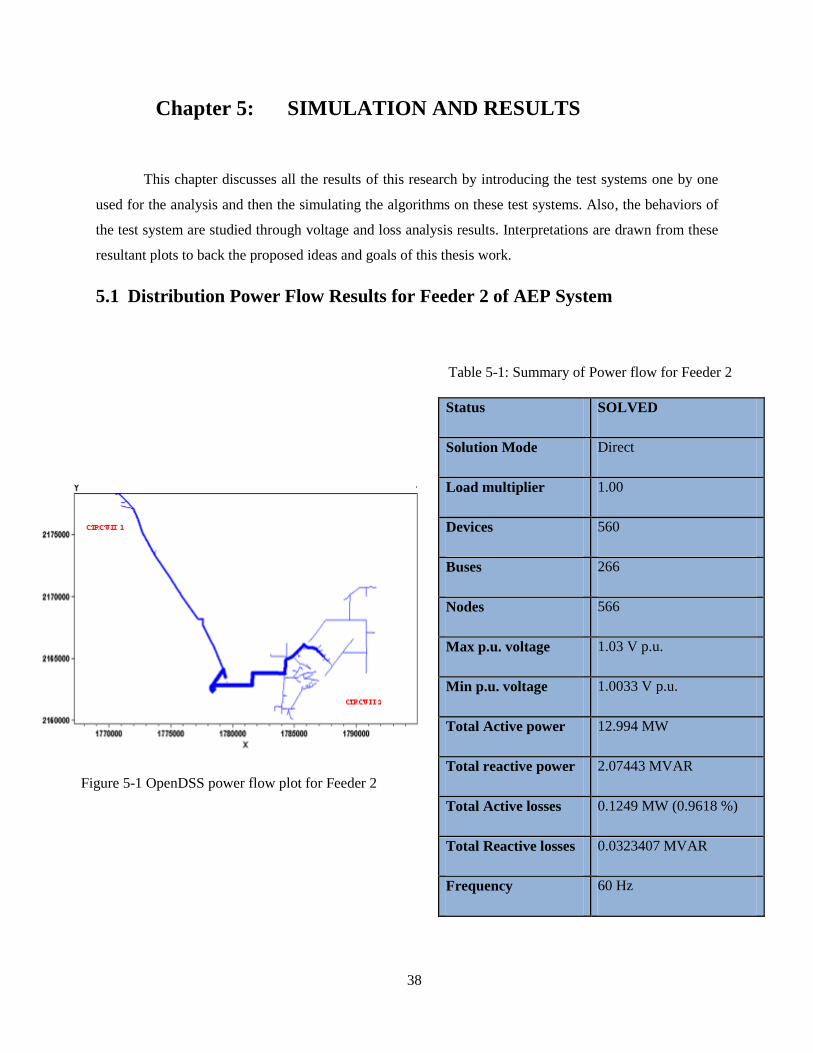
38
Chapter 5: SIMULATION AND RESULTS
This chapter discusses all the results of this research by introducing the test systems one by one
used for the analysis and then the simulating the algorithms on these test systems. Also, the behaviors of
the test system are studied through voltage and loss analysis results. Interpretations are drawn from these
resultant plots to back the proposed ideas and goals of this thesis work.
5.1 Distribution Power Flow Results for Feeder 2 of AEP System
Table 5-1: Summary of Power flow for Feeder 2
Status SOLVED
Solution Mode Direct
Load multiplier 1.00
Devices 560
Buses 266
Nodes 566
Max p.u. voltage 1.03 V p.u.
Min p.u. voltage 1.0033 V p.u.
Total Active power 12.994 MW
Total reactive power 2.07443 MVAR
Total Active losses 0.1249 MW (0.9618 %)
Total Reactive losses 0.0323407 MVAR
Frequency 60 Hz
Figure 5-1 OpenDSS power flow plot for Feeder 2

39
The Feeder 2 of AEP system is modeled in OpenDSS and a distribution power flow was run on it
and Figure 5-1 shows a one line diagram of feeder 2 resulted from OpenDSS. The distribution power flow
results for feeder 2 are listed in Table 5-1. Feeder 2 is a radial configuration and supplied by a 12.47 KV
medium voltage substation modeled as an infinite source. The distribution system comprises two main
circuits with laterals and distributed loads. A single 3-phase voltage regulator is employed in this feeder at
the substation. The system base is 100 MVA and 12.47 KV. PQ type loads are considered to model the
loads buses of the system. Seven different locations are considered along the feeder to place the Switched
capacitor banks. The loads of the system represent a mixture of residential and industrial loads and the
total load on the system is 13.15 MVA (12.994 MW and 2.074 MVAR) and the active power losses
represent 0.96 % of the total system load. The node voltages of feeder 2 are in the range of 1.003 V. p.u.
and 1.03 V. p.u.
5.2 PHEV Integration Study on Utility Distribution Feeder
The developed utility feeder 2 model is chosen for the PHEV integration study. Figure 5-2 shows
the AEP feeder with the PHEV charging stations and meter locations. Based on the data (number of
consumers and the distribution transformer ratings connected to these loads) provided by the utility, the
locations for placing the PHEV loads are identified and can be seen as green triangles in the feeder
diagram. The red dots in Figure 5-2 indicate the meters to analyze the system behavior (currents, voltages
and losses) during implementation of different charging strategies. The radial test feeder is supplied by a
12.47KV medium voltage substation modeled as an infinite source. Time series distribution power flow is
run for five different scenarios as follows.
• Scenario 1 – Without PHEVs: This is the base case distribution power flow with 24- hour
load shape considered for loads given by the utility.
• Scenario 2 – Uncoordinated Charging of PHEVs: In this case, the vehicles do not follow
any strategy to charge their batteries.
• Scenario 3 – Coordinated Charging of PHEVs with Maximum battery constraint: In this
case, the vehicles enroll in a charging strategy where the constraint (16) settles to the maximum battery
capacity.
• Scenario 4 – Coordinated Charging of PHEVs with Minimum battery constraint: In this
case, the vehicles enroll in a charging strategy where the constraint (16) settles to the minimum battery
capacity.

40
• Scenario 5 – Coordinated Charging with Demand Response: In this case, the vehicles
take part in a charging strategy involving DR programs. This strategy is discussed in detail in the
following section.
5.2.1 Specifications of PHEV Charging Station
Each PHEV has a maximum storage capacity of 22 kWh of which only 90% (i.e. 20kWh approx.)
is allowed to deteriorate during charge depletion mode to maintain optimal battery life. The vehicle can
travel a distance of 45 miles with this battery before entering the charge sustaining mode. The charging
station is assumed to equip with 100 charging slots keeping in view the popularity of the PHEVs. Here
even though 100 slots are available, the energizing of slots is a controlled action from the control center
based on the coordinated charging algorithm implies not all the connected vehicles get charged but
depends on the charging power decision matrix . The slot has a maximum power output of 3kW
(0.75kW per 15minutes interval) from a standard 230V AC outlet which is considered as Level 2
charging.
5.2.2 Uncoordinated Charging and Monte Carlo Simulation
To highlight the significance of proposed coordinated charging techniques, the system performance is
analyzed with uncoordinated charging at first. In uncoordinated charging scenario, the PHEVs are
Figure 5-2 AEP Feeder model with PHEV Charging Stations and meter locations

41
0 20 40 60 80 100 1200
100
200
300
400
500
600
State of Charge
Occura
nces
0 5 10 15 20 250
50
100
150
200
250
300
Hours
Charg
ing D
em
and (
KW
)
Vehicles away
from home
charged by connecting to the slots the very instant they arrive the CS and the slots were not controlled by
the control center.
Figure 5-3 MCS plot of State-of-Charge
Figure 5-4 MCS plot of Hourly Charging Demand

42
5.2.3 Coordinated Charging of PHEVs
The coordinated charging is achieved by giving the Monte-Carlo simulation results as inputs to
the optimization problem discussed. This setup is run in MATLAB for required number of time intervals
(depending on individual vehicle departure times) and the average computational time is 20 seconds when
run on a 2.2 GHz Intel Core 2 Duo CPU with 4.00 GB of RAM computer. The uncoordinated and
coordinated charging loads by the charging stations for 50% PHEV penetration specified in Table 5-2 are
evaluated using MATLAB and are given as hourly load multipliers for the OpenDSS and a 24-hour
distribution power flow is run to analyze the voltage response of the feeder. It is noticed that
uncoordinated charging causes the voltage at bus near to PHEV loads to reduce far below the lower limit
of 0.95 per unit as shown in Figure 5.5. Optimizing the PHEV charging loads with transformer constraint,
could potentially bring back the system voltage close to the limit. From hours 23:00 – 04:00 the voltage
profile of uncoordinated charging is better compared to coordinated (but well within the limits) as the
load curtailed during the peak hours is distributed to the later hours. Figure 5.6 gives the transformer
loading profile for scenarios 1 – 4 for CS 5. From equation (2), 90% of the vehicles reach home by 19:00,
and starts charging instantaneously causing a peak and overloading the transformer for next 3 to 4 hours.
The optimization avoids the overloading of the transformer, charges maximum number of vehicles
possible and maintains system stability.
Transformer
Rating (KVA) Base Load (KVA)
30% PHEVs
(Stochastic
Loading -kWh)
50% PHEVs
(Stochastic
Loading -kWh)
CS 1 150 81.469 31 (328) 52 (575)
CS 2 180 124.037 30 (320) 50 (591)
CS 3 140 66.124 12 (110) 20 (226)
CS 4 75 45.827 13 (130) 22 (248)
CS 5 200 61.102 56 (570) 94(1047)
Table 5-2. PHEV Penetration and Loading in the Test Feeder

43
0 5 10 15 20 250.92
0.94
0.96
0.98
1
1.02
1.04
1.06
Hours
B p
hase V
oltages(p
.u.)
Base case
Uncoordinated Charging
Coordinated Charging
0 5 10 15 20 250
50
100
150
200
250
300
350
Hours
Dem
and(k
VA
)
Base Load
Uncoordinated Charging
Optimized Charging
5.2.4 Voltage Profile of the Feeders
A 24 hour time series power flow is executed in OpenDSS with varying PHEV charging methods.
Figures 5-7 to 5-9 shows a comparison of the voltage profiles for different PHEV charging cases. The x-
axis of Fig. 5-7 to 5-9 represents the nodes from source to end of Lovell and Highland circuits, the y-axis
of Fig. 5-7 to 5-9 represent the hours of the day, and the z-axis of Fig. 5-7 to 5-9 represents the B-phase
Figure 5-5 Voltage profile for 24-hours of Feeder 2
Figure 5-6 Transformer loading for different charging methods

44
0
10
20
05
1015
20
0.95
1
1.05
Hours
Base Case Voltage
B P
hase V
olt
ag
e p
.u.
Source
Meter 0Source
Meter 0
End
Meter 6
End
Meter 19
voltages in p.u. Figure 5-7 shows the base case solution with no PHEV load present on the system,
indicating a wide range of voltages throughout the day owing to normal load variations. The surface plot
of Figure 5-7 indicates that there is no lower voltage deviation from limits of 0.95 p.u for base case
solution.
The voltage of the test feeder for uncoordinated charging is shown in Figure 5-8. Plot indicates a
significant voltage drop in the Highland circuit (where the loads are purely residential) during the peak
hours as the PHEV owners connect the vehicles as soon as they arrive home. This voltage instability
motivates the distribution system operators to design efficient charging methods to satisfy the customers
as well as maintain the voltage of the system well within limits.
Figure 5-7 Feeder 2 Voltage Profile - Base Case

45
0
10
20
05
1015
20
0.95
1
1.05
Hours
Uncontrolled Charging Voltage Profile
B P
hase V
olt
ag
e p
.u.
Source
Meter 0
End
Meter 6Lovell
Source
Meter 0 End
Meter 19Highland
0
10
20
05101520
0.95
1
1.05
Hours
Voltage Profile with Optimized Charging
B P
hase V
olt
ag
e p
.u.
End
Meter 19
Source
Meter 0 End
Meter 6
Source
Meter 0
Figure 5-9 shows improvement in the voltage profile of the test feeder when a coordinated
charging method is implemented on the PHEVs connected to the local utility. Smart charging methods
not only help in energy management but also assist in maintaining system voltages well within limits.
Figure 5-8 Feeder 2 Voltage Profile - Uncoordinated Charging
Figure 5-9 Feeder 2 Voltage Profile - Coordinated Charging

46
5.2.5 Load Profiles of Distribution Transformers
This section deals with study on extent of transformers capability to support the coordinated
charging algorithm. Two transformers are considered with different capacities and number of customers
supplied by the corresponding transformers. Table 5-3 gives the transformer information.
Table 5-3: Transformer Loading Analysis
Load Name Bus Name Transformer
Rating
Load
Rating
Number of
PHEVs
216_7231506-1 fict26_HIGHLAND.3 200 61.102 94
359_7231506-1 fict20_HIGHLAND.3 140 66.194 20
(a) (b)
The loading patterns of considered transformers are shown in Figures 5-10 (a) and (b).
Coordinated charging methods are implemented at charging stations (CS) supplied by the transformers
with capacity less than required to support the PHEV customers connected to it. Figure 5-10 (a) clearly
indicates this particular CS needs coordinated charging algorithm in order to protect the transformer from
0 5 10 15 20 250
50
100
150
200
250
300
350
Hours
Dem
and(k
VA
)
Distribution Tranformer Loading
Base Load
Un-coordinated Charging
Optimized Charging
0 5 10 15 20 2540
60
80
100
120
140
160
Hours
Dem
and(k
VA
)
Distribution Tranformer Loading
Base Load
Un-coordinated Charging
Optimized Charging
Figure 5-10 Distribution Transformer Loading Patterns

47
excess load due to PHEVs and thereby improving the life of transformer. The charging algorithm with a
constraint on transformer capacity avoids peaks and extends the duration of PHEV charging to late hours
of the night.
Transformers with sufficient capacity to support the customers charging needs need not
participate in the charging algorithms. Figure 5-10 (b) shows the charging demand does not overload the
transformer and the uncoordinated charging and coordinated charging curves coincide with each other.
Such CS can also implement the coordinated charging methods by enforcing a less transformer capacity
constraint which has the chance of delaying the charging needs of the customers.
5.2.6 Comparison between Scenarios 3 and 4
Scenario 4 (Coordinated Charging of PHEVs with Minimum battery constraint) is a strategy
aimed at charging maximum number of PHEVs rather than charging limited number of PHEVs with
maximum possible charging rate. The drawback of scenario 3 is that, the few vehicles arriving early to the
CS or vehicles which are fed first to the optimization algorithm gets charged faster whereas the late
arriving vehicles take much time to completely charge than average. This drawback can be overcome to
some extent using scenario 4. The transformer load shape for these scenarios is expressed as a single
coordinated charging curve because the energy consumption remains the same with the number of
vehicles getting charged varies. It is also noticed that vehicles charging with scenario 4 are not left far
behind in terms of SOC as shown in Figure 5-11. Three vehicles are chosen randomly and time taken to
reach 70% SOC is computed which shows scenario 4 is also an ideal strategy to charge the PHEVs.
Figure 5-11 Time taken by random vehicles to reach 70% SOC
0 5 10 15
AT
-16
:00 (
SO
C
10
%)
AT
-17
:00 (
SO
C
10
%)
AT
-18
:00 (
SO
C
50
%)
(a) Hours
Scenario 4
Scenario 3

48
Figure 5-12 Battery capacities of late arrival vehicles
Scenario 4 is designed such that if the customer desires to leave early or has unplanned departure,
this strategy has the advantage of improved state of charge from initial arrival SOC when compared to
scenario 3. This is well explained in Figure 5-12 using a set of vehicles which arrived at CS after hour
19:00 with random initial SOCs. The battery states improved with scenario 4 due to early start of
charging when compared with the unaltered states of scenario 3.
5.2.7 Demand Response Application
The coordinated charging algorithm satisfies the main objective of avoiding overloading of
distribution transformer during times of heavy inrush of PHEVs. But, the transformer is loaded 100% for
more hours added to the peak hours as shown in Figure 5-6. As discussed in section III, DR helps at times
of system emergencies by providing incentives to the consumers. The charging station reserves special
slots for PHEV customers who are willing to take part in DR programs mostly encouraging the customers
with lengthier parking times showing the hourly real time prices and cost benefits incurred due to late
charging. The DR program is a self-prioritization algorithm in which the customers enroll themselves by
placing the vehicles in the special slots which facilitates late charging thereby the remaining slots will be
occupied with vehicles requiring early charging i.e. the slot matrix with priority vehicles is
supplied to the coordinated charging algorithm. This strategy has the advantage of satisfying customers
with early charging needs and also reduces the transformer loading by efficiently utilizing the extended
low-price parking hours of vehicles as shown in Figure 5-13.
0 5 10 15 20
1
2
3
4
5
6
7
8
9
10
Battery Capacity (kWh)
Vehicle
Scenario 4
Scenario 3

49
0 5 10 15 20 250
50
100
150
200
250
300
350
Hours
Dem
and(k
VA
)
Base Load
Uncoordinated Charging
Optimized Charging
DR Application
5.3 PRT Distribution System Analysis
The routing algorithm discussed in section VI is run as a MILP in MATLAB environment based
on the passenger data provided by WVU DOT for a single day which is a normal university working day.
The data consists of number of passengers travelling between all the possible station pairs, distance and
time taken by a vehicle to commute between these stations. Figure 5-14 shows the hourly accumulated
passenger demand at all the 5 stations starting from 07:00 till 22:15 (hours of operation of PRT). Each
station has its own peak and off-peak demand hours depending on the locality, for instance, the Beechurst
Avenue for the Downtown campus is the main campus and having more student traffic followed by
Engineering Sciences station. Average energy consumption by a vehicle is 1kWh/mi and 80kWh battery
capacity is considered to be installed in the BEVs. The minimum number of BEVs required to transport
the passengers at each station pair for each hour is obtained on running the routing algorithm and is
shown in Figure 5-15.
Figure 5-13 Transformer loading for different charging methods - with Demand Response

50
Figure 5-14 Hourly passenger demand at all 5 stations
Figure 5-15 Number of vehicles at each station pair
The routing algorithm along with calculating the minimum number of vehicles also keeps track of
the battery capacity of each departed vehicle. Hourly charging demand and charging demand at the end of
day on distribution system are computed for two cases –
Case 1 – Three station charging
0
100
200
300
400
500
600
700
800
900
7:00 8:00 9:00 10:00 11:00 12:00 13:00 14:00 15:00 16:00 17:00 18:00 19:00 20:00 21:00 22:00 22:15
Nu
mb
er o
f S
tud
ents
Hours
Hourly Students Demand – All Stations
Walnut Beechrust Engineering Towers Health Scs
0
2
4
6
8
10
7:00 8:00 9:00 10:00 11:00 12:00 13:00 14:00 15:00 16:00 17:00 18:00 19:00 20:00 21:00 22:00 22:15
Nu
mb
er o
f V
ehic
les
Hours
Optimized Number of Vehicles between Pair of Stations
Walnut - Beechrust Walnut - Engineering Walnut - Towers
Walnut - Health Scs Beechrust - Engineering Beechurst - Towers

51
Case 2 – All station charging
The stations are equipped with charging infrastructure and the transformer ratings (575V AC, 3-
phase) at the stations are suitable for providing fast charging which can charge the BEVs in one hour. The
test system discussed in section VII is considered to perform the distribution system analysis with slight
modifications of adding additional transformers at nodes coinciding with geographical location of
physical stations as shown in Figure 5-16. In case 1, the intermediate stations - Beechurst, Engineering
Sciences and Evansdale Residential Complex are chosen for charging BEVs as these stations has large
student demand and require more vehicles.
Number of BEVs available (i.e. total – charging) for service in next hour are fed to the algorithm
as ) in constraint (18). The BEVs enter the service with full charging and for the demand
shown in Figure 5-14, the first group of vehicles charge at 12:00 and as the peak charging occurs at 14:00
as shown in Figure 5-17. BEVs are assumed to charge only if the battery capacity reaches below a
threshold limit and not during their ideal or non-service hours because repeated charging and discharging
potentially depletes battery life-time. The threshold limit is decided based on hourly energy consumption
of vehicle since once the vehicle enters the service, it must be capable of running for duration of one
complete hour. The charging demand on the test feeder along with residential and industrial load is shown
in Figure 5-18. The charging demand in both the cases 1 and 2 remains the same except the demand is
distributed to more nodes in the latter case which has considerable effect on the voltage of the system
Figure 5-16 AEP Feeder-2 with PRT Stations

52
0 5 10 15 20 250
1000
2000
3000
4000
5000
6000
7000
8000
9000
Load Demand
Hours
Lo
ad
(k
W)
Base Load
PRT Charging Demand
when the passenger demand is too high. A more distribution of charging demand can be achieved by
using batteries with fewer capacities which can avoid peaks on the distribution system.
Figure 5-17 Total number of BEVs in Service and Charging modes
0
5
10
15
20
25
30
35
40
45
Nu
mb
er o
f B
EV
s
Hours
Vehicle Analysis
BEVs in Service BEVs in Charging
Figure 5-18 Base load and charging load of AEP distribution feeder

53
2 6 10 14 18 22 240.92
0.94
0.96
0.98
1
1.02
1.04
1.06
1.08Phase-A
Voltage Profile
Hours
Vo
ltag
e (
p.u
)
Feeder HeadTo
End Node
1 2 3 4 5 6 7 8 90.97
0.99
1.01
1.03
1.05
1.06
Vo
ltag
e (
p.u
)
Towards Beechurst - Walnut
Towards Engineering-Towers - Health Sc
Case - 2
Case - 1
Normal Load Hours
PRT Load Hours
Feeder Head End Node
By the end of service, BEVs are charged completely based on availability of slots shown in
Figure 5-18 as peaks during end hours. The voltage profile of the metered nodes of the feeder is given in
Figure 5-19. In order to examine the effects of case-2 on the distribution feeder, the routing algorithm is
run with assumed large passenger demand which increases the charging demand and significantly affects
the voltage of the feeder during peak hours. Figure 5-20 indicates the improvement in voltage profile
when BEV charging is distributed among all the stations. Voltage from feeder head towards end nodes
including the station nodes for normal load demand and PRT peak demand hours is plotted in Figure 5-
20.
Figure 5-19 Voltage profile for 24-hours at all metered locations
Figure 5-20 Voltage profile of Case-1 and 2

54
5.4 PHEV Impacts on LMPs
A DCOPF on modified IEEE 13 Node test system is run in MATLAB environment for 24-hour
time period and the effects of PHEV charging demand on system LMPs is discussed in this section. The
dual variables of equality constraints in the optimization provide the locational marginal prices at all the
13 nodes of the system. 7 generators shown as ‘G’ with different price curves at different nodes as shown
in Figure 5-21 are considered for the analysis which are a mixture of conventional and distributed
generators . The low cost generation comes from renewables like PV and wind, and generators like gas
turbine are expensive. The bid prices and capacities of generators are given in Table 5-4. Loads capable
of creating congestion in the system are considered to notice the variations of prices at different nodes and
are given in Table 5-5. The line flow limit is considered as 500MVA for all the lines for convenient
analysis.
The LMPs for 24-hours at few of the nodes for base load is shown in Figure 5-22. 5 nodes are
selected to notice the prices of the system. Node 645 which is near to the costly generator under goes
large variation in the prices. The prices are quite low – following the least cost generator till a certain
level of loading and as the system experiences high load, due to congestion the prices are influenced by
the high cost generator. Figure 5-22 clearly indicates the change in prices at different nodes of the system.
Figure 5-21 IEEE 13 Node Test Feeder

55
Due to uncoordinated charging of PHEVs by the owners at times of already existing peaks, the
load on the system increases manifold causing congestion and increase in the prices. Under these
conditions, the normal base load of the system is also charged at higher prices along with the new PHEV
load. Node 675 is considered to study the effects of PHEV charging on market prices. Figure 5-23 shows
the variation in prices caused by uncoordinated charging which creates congestion in the system. It is also
shown that coordinated charging of PHEVs discussed in prior sections has a significant effect on the
market prices by distributing the peak load to off-peak hours and thereby avoiding congestion.
Table 5-4: Generator Data
Table 5-5: Load Data
Generators Bidding Price
($/MWH)
Maximum
Capacity(MW)
Generator-650 10 600
Generator-646 40 300
Generator-634 14 410
Generator-611 30 520
Generator-671 20 600
Generator-675 25 500
Generator-680 35 800
Load Rating (MW)
L-675 100
L-646, L-633, L-692 200
L-645, L-634 300
L-684, L-671 400
L-652 500

56
0 5 10 15 205
10
15
20
25
30
35
40
45
Hours
LM
P
Node-650
Node-645
Node-633
Node-675
Node-671
0 5 10 15 20 25
0.7
0.8
0.9
1
1.1
1.2
1.3
1.4
1.5
Hours
Multip
lier
Figure 5-22: 24-hour multiplier for load nodes
Figure 5-23: LMPs at Different Nodes

57
0 5 10 15 20 255
10
15
20
25
30
35
40
45
Hours
LM
P
Base Case
Uncoordinated Charging
Coordinated Charging
Figure 5-24: PHEV Charging Effects on LMP

58
Chapter 6: CONCLUSION AND FUTURE WORK
6.1 Conclusion
In this thesis, a charging algorithm has been formulated for charging stations at residential
complexes with the objective of charging as many vehicles as possible. A demand response application
for charging of PHEVs is also implemented to enhance the longevity of the distribution system. Further,
an efficient routing algorithm is designed for transit system to test the power system feasibility when
converted into BEVs. The conclusions drawn from both these works have been presented in this section.
6.1.1 Coordinated Charging Method
In this thesis, a coordinated charging strategy for a Charging Station (CS) in the direction of maximizing
the number of PHEVs charged by formulating a Mixed Integer Linear Programming (MILP)
Optimization in MATLAB. The effects of coordinated charging methods on utility distribution system are
analyzed using OpenDSS. PHEV customers are modeled into price responsive consumers capable of
participating in Demand Response programs by developing extensive demand-price elasticity matrices
(PEMs) which are utilized to calculate the level of demand response.
Results indicate that coordinated charging strategies impacts the distribution network in 3 positive ways:
1. Voltage profile improvement
2. Loss minimization
3. Valley filling
4. Customer satisfaction
6.1.2 PRT Routing Algorithm
The feasibility of converting the guideway power rail propelling vehicles to Battery driven
vehicles (BEVs) by developing a novel routing algorithm based on scheduled mode of operation from the
data provided by the West Virginia University’s Department of Transportation and Parking is well
accomplished by analyzing the voltage and loading of the distribution feeder due to the hourly charging
demand of BEVs. This has been done by formulating an optimization in MATLAB to find optimal
number of BEVs required to satisfy the student demand on a normal university working day.
The vehicles available at the stations can provide grid support during the peak demand hours and the
BEVs can be charged with renewables integrated with the charging stations.

59
6.2 Future Work
PHEVs are gaining popularity both in terms of economic and environment benefits. Tax
incentives provided by the government and also reduced fuel cost per mile are the driving forces. With the
advent of advanced communication and control techniques in the grid, PHEVs promises immense benefits
to both electric utilities and consumers. Integration of PHEVs with grid called V2G technology is the area
gaining a lot of research interest. Designing of charging stations with renewable energy sources is also
feasible in the near future. Providing ancillary services to the grid in terms of frequency control is a
promising application of PHEVs. Future work will focus on gathering real time data on customer
participation in DR programs and imparting a customer satisfaction parameter in objective function.
Designing coordinated charging and communication algorithms for complex systems such as charging at
home garages needs to be focused.
BEVs offer similar advantages as PHEVs. The main application lies in treating the BEVs as
mobile storage units providing V2G in larger scale than PHEVs due to their huge battery size. Many
transit systems are in the process of converting guideway propelled vehicles to BEVs due to zero
maintenance of the guideways offered by the BEVs. The aggregated battery storage of BEVs finds
applications in microgrid applications. A comprehensive routing algorithm involving the intermediate
stations irrespective of station pairs with the objective of minimizing the charging demand needs to be
formulated. Minute wise scheduling of the vehicles with additional collision constraints is considered as
next step in accurate analysis of energy consumption. Detailed economics related to setting up charging
infrastructure at PRT stations and converting into BEVs have to be evaluated to test the feasibility of this
conversion project.

60
References
1. “Title XIII - Smart Grid, Sec. 1301, Statement of Policy on Modernization of Electricity Grid”,
Energy Independence and Security Act of 2007 (EISA), USA.
2. http://info.ornl.gov/sites/publications/files/Pub14078.pdf
3. J.A. Schellenberg, M.J. Sullivan, “Electric vehicle forecast for a large West Coast utility,” in
Proc. 2011 IEEE Power & Energy Society General Meeting, pp. 1-6.
4. http://www.iea.org/topics/transport/electricvehiclesinitiative/EVI_GEO_2013_Timeline.PDF
5. Ahman, M. (2001). Primary energy efficiency of alternative powertrains in vehicles. Energy 26:
973-989.
6. http://dspace.mit.edu/bitstream/handle/1721.1/54532/565948939.pdf?...1
7. N. Shidore, J. Kwon, A. Vyas, “Trade-off between PHEV fuel efficiency and estimated battery
cycle life with cost analysis”, in Proc. 2009 IEEE Vehicle Power and Propulsion Conference, pp
669 – 677.
8. http://www1.eere.energy.gov/vehiclesandfuels/avta/pdfs/phev/climate_leadership_conf_may09.p
df
9. P. Khajavi, H. Abniki, A.B. Arani, “The role of incentive based Demand Response programs in
smart grid”, in Proc. 2011 International Conference on Environment and Electrical Engineering,
pp. 1-4.
10. Federal Energy Regulatory Commission, United States, “Preventing Undue Discrimination and
Preference in Transmission Service,” [online] http://www.ferc.gov/whats-new/comm-
meet/091505/E-1.pdf
11. http://evworld.com/news.cfm?newsid=28119
12. M. Duoba, R. Carlson, and D. Bocci, “Calculating results and performance parameters for
PHEVs,” presented at the SAE World Congr. Exhib., Detroit, MI, Apr. 2009, 2009-01-1328.
13. K. Morrow, D. Karner, and J. Francfort, “Plug-In Hybrid Electric Vehicle Charging Infrastructure
Review,” Idaho National Laboratory, INL/EXT-08-15058, 2008. [Online]. Available:
http://avt.inel.gov/pdf/phev/phevInfrastructureReport08.pdf. [Accessed: Apr. 7, 2009].
14. M. D. Galus, G. A. Simon Art, “A hierarchical, distributed PEV charging control in low voltage
distribution grids to ensure network security,” in Proc. 2012 IEEE Power & Energy Society
General Meeting, pp. 1-8.
15. S. Shengnan, M. Pipattanasomporn, S. Rahman, “Challenges of PHEV penetration to the
residential distribution network,” in Proc. 2009 IEEE Power & Energy Society General Meeting,
pp. 1-8.

61
16. Z. Darabi, M. Ferdowsi, “Extracting probability distribution functions applicable for PHEVs
charging load profile,” in Proc.2012 IEEE Transmission and Distribution Conference and
Exhibition Conf., pp.1-6.
17. Y. Yin, D. W. Gao, “Charging load from large-scale plug-in hybrid electric vehicles: Impact and
optimization,” in Proc. 2013 IEEE Innovative Smart Grid Technologies Conf.pp.1-6.
18. Tae-Kyung Lee, B. Adornato, Z.S. Filipi,Jones, “Synthesis of Real-World Driving Cycles and
Their Use for Estimating PHEV Energy Consumption and Charging Opportunities: Case Study
for Midwest/U.S.,”IEEE Trans. Vehicular Tech., vol. 60, no. 9, pp. 4153-416 3, Dec. 2011.
19. D. Steen, L. A. Tuan, O. Carlson, L. Bertling, "Assessment of Electric Vehicle Charging
Scenarios Based on Demographical Data," IEEE Trans. Smart Grid, vol. 3, no. 3, pp. 1457-1468.
20. M. Yilmaz, P. T. Krein, “Review of charging power levels and infrastructure for plug-in electric
and hybrid vehicles ,” in Proc. 2012 IEEE Electric Vehicle Conf. pp. 1-8.
21. S. Acha, T. C. Green, N. Shah, “Effects of optimized plug-in hybrid vehicle charging strategies
on electric distribution network losses,” in Proc.2010 IEEE Transmission and Distribution
Conference and Exposition Conf., pp.1-6.
22. E. Sortomme, M. M. Hindi, S. D. J. MacPherson, S. S. Venkata, “Coordinated Charging of Plug-
In Hybrid Electric Vehicles to Minimize Distribution System Losses,” IEEE Trans. Smart Grid,
vol. 2, no. 1, pp. 198-205, Feb 2011.
23. D. S. Deilami, A. S. Masoum, P. S. Moses, M. A. S. Masoum, “Real-Time Coordination of Plug-
In Electric Vehicle Charging in Smart Grids to Minimize Power Losses and Improve Voltage
Profile,” IEEE Trans. Smart Grid, vol. 2, no. 3, pp. 456-467.
24. N. Fettinger, T. Chee-Wooi, C. Chunxiao, “Minimizing residential distribution system operating
costs by intelligently scheduling plug-in hybrid electric vehicle charging,” in Proc. 2012 IEEE
Transportation Electrification Conf. and Expo., pp. 1-8.
25. M. Hajian, S. Manish, H. Zareipour, W. D. Rosehart, “Investigation of enabling wind generations
employing plug-in hybrid electric vehicles,” in Proc. 2012 IEEE Power & Energy Society
General Meeting, pp. 1-7.
26. Xin Li, L. A. C. Lopes, S. S. Williamson, “On the suitability of plug-in hybrid electric vehicle
(PHEV) charging infrastructures based on wind and solar energy,” in Proc. 2009 IEEE Power &
Energy Society General Meeting, pp. 1-8.
27. O. Hafez, K. Bhattacharya, “Optimal PHEV charging in coordination with distributed generation
operation in distribution systems,” in Proc. 2012 IEEE Power & Energy Society General Meeting,
pp. 1-7.

62
28. S. Shengnan, M. Pipattanasomporn, S. Rahman, “Demand Response as a Load Shaping Tool in
an Intelligent Grid With Electric Vehicles,” IEEE Trans. Smart Grid, vol. 2, no. 4, pp. 624-631.
29. M. Erol-Kantarci, H. T. Mouftah, “Management of PHEV batteries in the smart grid: Towards a
cyber-physical power infrastructure,” Wireless Comm. And Mobile Comp. Conf., pp. 795-800.
30. S. Wencong, C. Mo-Yuen, “Performance evaluation of a PHEV parking station using Particle
Swarm Optimization,” in Proc. 2011 IEEE Power & Energy Society General Meeting, pp. 1-6.
31. http://ens-newswire.com/2013/10/09/first-u-s-charging-station-for-all-evs-opens-in-california/
32. https://suncountryhighway.ca/worlds-longest-greenest-highway-project/
33. http://www.chargepoint.com/
34. L. Turcksin, S. Van Moll, C. Macharis, N. Sergeant, and J. Van Mierlo, “How green is the car
purchase decision? A review,” in 10th Int. Conf. Applic. Adv. Techn. Transportation, Athens,
Greece, 27-31 May 2008
35. U.S. Dept. of Transportation, Federal Highway Administration. National household travel survey
(NHTS). [Online]. Available:http://nhts.ornl.gov/download.shtm
36. Caramanis, M.C., Bohn, R.E., Schweppe, F.C., “Optimal Spot Pricing: Practice and Theory”,
IEEE Transactions on Power Apparatus and Systems, vol. PAS-101, no. 9, Sept. 1982, pp: 3234-
3245.
37. Schweppe F.C., Caramanis, M.C., Tabors, R.D., Bohn, R.E., “Spot Pricing of Electricity”,
Boston, MA: Kluwer, 1988.
38. Schweppe, F.C., Caramanis, M.C., Tabors, R.D., “Evaluation of Spot Price Based Electricity
Rates”, IEEE Transactions on Power Apparatus and Systems, vol. PAS-104, no. 7, July 1985,
pp.1644-1655.
39. David, A.K., Li, Y.Z., “Consumer Rationality Assumptions in the Real Time Pricing of
Electricity”, Proceedings of the IEEE conference on Advances in Power System Control,
Operation and Management, Hong Kong, Nov 1991.
40. David, A.K., Lee Y.C., “Dynamic Tariffs: Theory of Utility-Consumer Interaction”, IEEE
Transactions on Power Systems, vol. 4, no. 3, Aug 1989, pp: 904-911.
41. David, A.K., Li, Y.Z., “Effect of Inter-Temporal Factors on the Real Time Pricing of Electricity”,
IEEE Transactions on Power Systems, vol. 8, no. 1, Feb 1993, pp: 44-52.
42. M. Mallette, G. Venkataramanan, “The role of plug-in hybrid electric vehicles in demand
response and beyond,” in Proc.2010 IEEE Transmission and Distribution Conference and
Exposition Conf., pp.1-7.

63
43. S. Shengnan,Z. Tianshu, M. Pipattanasomporn, S. Rahman, “Impact of TOU rates on distribution
load shapes in a smart grid with PHEV penetration,” in Proc.2010 IEEE Transmission and
Distribution Conference and Exposition Conf., pp.1-6.
44. V. Naveen, S. Jignesh, S.K. Sarika, “Residential Demand Response model and impact on voltage
profile and losses of an electric distribution network,” in 2012 Proc. Applied Energy, vol 96, pp.
84-91
45. https://transportation.wvu.edu/prt/facts_about_the_prt
46. S.G. Wirasingha, N. Schofield, A. Emadi, “Feasibility analysis of converting a Chicago Transit
Authority (CTA) transit bus to a plug-in hybrid electric vehicle,” Vehicle Power and Propulsion
Conference, 2008, pp. 1-7.
47. P. Vishnu, R. Ajaykrishna, S. Thirumalini, “Cost effective energy solution with dual battery for
plug-in hybrid electric vehicle (PHEV) in a public transportation system,” in IEEE Conf. 2012 on
Industrial Electronics and Applications (ICIEA), pp. 1555-1560.
48. http://transportation.wvu.edu/r/download/18440
49. OpenDSS Manual, Electric Power Research Institute, Jul 2010. Available:
http://sourceforge.net/projects/electricdss/
50. http://www.smartgrid.epri.com/doc/OpenDSS Level 1 Training.pdf
51. The MathWorksTM
, http://www.mathworks.com/products/matlab/description1.html
52. http://www-01.ibm.com/software/integration/optimization/cplex-optimizer/