SANDIA REPORTSAND2015-2461Unlimited ReleasePrinted April 2015

Modeling an Application’s TheoreticalMinimum and Average TransactionalResponse Times

Mary Rose Paiz

Prepared bySandia National LaboratoriesAlbuquerque, New Mexico 87185 and Livermore, California 94550

Sandia National Laboratories is a multi-program laboratory managed and operated by Sandia Corporation,a wholly owned subsidiary of Lockheed Martin Corporation, for the U.S. Department of Energy’sNational Nuclear Security Administration under contract DE-AC04-94AL85000.

Approved for public release; further dissemination unlimited.

Issued by Sandia National Laboratories, operated for the United States Department of Energyby Sandia Corporation.

NOTICE: This report was prepared as an account of work sponsored by an agency of the UnitedStates Government. Neither the United States Government, nor any agency thereof, nor anyof their employees, nor any of their contractors, subcontractors, or their employees, make anywarranty, express or implied, or assume any legal liability or responsibility for the accuracy,completeness, or usefulness of any information, apparatus, product, or process disclosed, or rep-resent that its use would not infringe privately owned rights. Reference herein to any specificcommercial product, process, or service by trade name, trademark, manufacturer, or otherwise,does not necessarily constitute or imply its endorsement, recommendation, or favoring by theUnited States Government, any agency thereof, or any of their contractors or subcontractors.The views and opinions expressed herein do not necessarily state or reflect those of the UnitedStates Government, any agency thereof, or any of their contractors.

Printed in the United States of America. This report has been reproduced directly from the bestavailable copy.

Available to DOE and DOE contractors fromU.S. Department of EnergyOffice of Scientific and Technical InformationP.O. Box 62Oak Ridge, TN 37831

Telephone: (865) 576-8401Facsimile: (865) 576-5728E-Mail: reports@adonis.osti.govOnline ordering: http://www.osti.gov/bridge

Available to the public fromU.S. Department of CommerceNational Technical Information Service5285 Port Royal RdSpringfield, VA 22161

Telephone: (800) 553-6847Facsimile: (703) 605-6900E-Mail: orders@ntis.fedworld.govOnline ordering: http://www.ntis.gov/help/ordermethods.asp?loc=7-4-0#online

DE

PA

RT

MENT OF EN

ER

GY

• • UN

IT

ED

STATES OFA

M

ER

IC

A

2

SAND2015-2461Unlimited ReleasePrinted April 2015

Modeling an Application’s Theoretical Minimum andAverage Transactional Response Times

Mary Rose Paiz

Application Services and Analytics

Sandia National Laboratories

MS 1465

Albuquerque, NM 87123

Abstract

The theoretical minimum transactional response time of an application serves as a ba-sis for the expected response time. The lower threshold for the minimum response timerepresents the minimum amount of time that the application should take to complete atransaction. Knowing the lower threshold is beneficial in detecting anomalies that are re-sults of unsuccessful transactions. On the converse, when an application’s response timefalls above an upper threshold, there is likely an anomaly in the application that is causingunusual performance issues in the transaction. This report explains how the non-stationaryGeneralized Extreme Value distribution is used to estimate the lower threshold of an ap-plication’s daily minimum transactional response time. It also explains how the seasonalAutoregressive Integrated Moving Average time series model is used to estimate the upperthreshold for an application’s average transactional response time.

3

Acknowledgment

I am thankful to my manager, Greg N. Conrad, and members of the Application Servicesand Analytics Department, for their constant guidance and support throughout my researchand analysis.

4

Contents

Nomenclature 11

1 Introduction 13

Motivation . . . . . . . . . . . . . . . . . . . . . . . . . . . . . . . . . . . . . . . . . . . . . . . . . . . . . . . . . . . 13

Middleware Applications . . . . . . . . . . . . . . . . . . . . . . . . . . . . . . . . . . . . . . . . . . . . . . . 14

Oracle eBusiness Suite Application . . . . . . . . . . . . . . . . . . . . . . . . . . . . . . . . . . . 14

Weblogic 12c Server Application . . . . . . . . . . . . . . . . . . . . . . . . . . . . . . . . . . . . . 14

Method . . . . . . . . . . . . . . . . . . . . . . . . . . . . . . . . . . . . . . . . . . . . . . . . . . . . . . . . . . . . . 15

2 Time Series 17

Introduction . . . . . . . . . . . . . . . . . . . . . . . . . . . . . . . . . . . . . . . . . . . . . . . . . . . . . . . . . 17

Stationarity . . . . . . . . . . . . . . . . . . . . . . . . . . . . . . . . . . . . . . . . . . . . . . . . . . . . . . . . . . 19

Stationarity in a Time Series Process . . . . . . . . . . . . . . . . . . . . . . . . . . . . . . . . . 19

Graphical Check of Stationarity . . . . . . . . . . . . . . . . . . . . . . . . . . . . . . . . . . . . . 20

Algebraic Check of Stationarity . . . . . . . . . . . . . . . . . . . . . . . . . . . . . . . . 23

Removing Non-Stationarity . . . . . . . . . . . . . . . . . . . . . . . . . . . . . . . . . . . . . . . . . 25

3 Extreme Values in a Time Series Process 29

Extreme Value Theory - Stationary . . . . . . . . . . . . . . . . . . . . . . . . . . . . . . . . . . . . . . . 29

Order Statistics . . . . . . . . . . . . . . . . . . . . . . . . . . . . . . . . . . . . . . . . . . . . . . . . . . . 29

Generalized Extreme Value Distribution . . . . . . . . . . . . . . . . . . . . . . . . . . . . . . . 30

Extreme Value Theorem for Stationary Time Series Processes . . . . . . . 31

Block Minima Method . . . . . . . . . . . . . . . . . . . . . . . . . . . . . . . . . . . . . . . 32

5

Estimating Parameters . . . . . . . . . . . . . . . . . . . . . . . . . . . . . . . . . . . . . . . 33

Extreme Value Theory - Non-Stationary . . . . . . . . . . . . . . . . . . . . . . . . . . . . . . . . . . . 34

Non-Stationary Generalized Extreme Value Distribution . . . . . . . . . . . . . . . . . 34

Model Selection . . . . . . . . . . . . . . . . . . . . . . . . . . . . . . . . . . . . . . . . . . . . . . . . . . . . . . . 35

4 Modeling Time Series 39

Introduction . . . . . . . . . . . . . . . . . . . . . . . . . . . . . . . . . . . . . . . . . . . . . . . . . . . . . . . . . 39

Non-Mixed Models . . . . . . . . . . . . . . . . . . . . . . . . . . . . . . . . . . . . . . . . . . . . . . . . . . . . 39

Autoregressive Model: AR(p) . . . . . . . . . . . . . . . . . . . . . . . . . . . . . . . . . . . . . . . 39

Moving Average Model: MA(q) . . . . . . . . . . . . . . . . . . . . . . . . . . . . . . . . . . . . . 41

Forecast Function . . . . . . . . . . . . . . . . . . . . . . . . . . . . . . . . . . . . . . . . . . . . . . . . . 42

Mixed Models . . . . . . . . . . . . . . . . . . . . . . . . . . . . . . . . . . . . . . . . . . . . . . . . . . . . . . . . 43

Autoregressive Moving Average Model: ARMA(p, q) . . . . . . . . . . . . . . . . . . . . 43

Autoregressive Integrated Moving Average Model: ARIMA . . . . . . . . . . . . . . 44

Non-Seasonal ARIMA(p, q, d) Model . . . . . . . . . . . . . . . . . . . . . . . . . . . 44

Seasonal ARIMA(p, q, d)[P,D,Q][s] Model . . . . . . . . . . . . . . . . . . . . . . 45

Model Selection . . . . . . . . . . . . . . . . . . . . . . . . . . . . . . . . . . . . . . . . . . . . . . . . . . . . . . . 46

Saturated Model. . . . . . . . . . . . . . . . . . . . . . . . . . . . . . . . . . . . . . . . . . . . . . . . . . 46

Estimation and Forecasting of ARIMA Models . . . . . . . . . . . . . . . . . . . . . . . . . 47

5 Implementation To Oracle eBusiness Suite Application 49

Introduction . . . . . . . . . . . . . . . . . . . . . . . . . . . . . . . . . . . . . . . . . . . . . . . . . . . . . . . . . 49

Daily Minimum Transactional Response Time . . . . . . . . . . . . . . . . . . . . . . . . . . . . . . 49

Checking for Stationarity . . . . . . . . . . . . . . . . . . . . . . . . . . . . . . . . . . . . . . . . . . . 49

Block Minima Method . . . . . . . . . . . . . . . . . . . . . . . . . . . . . . . . . . . . . . . . . . . . . 50

Selection of Time Dependent Parameters . . . . . . . . . . . . . . . . . . . . . . . . . . . . . . 51

Estimating the non-stationary GEV Distribution . . . . . . . . . . . . . . . . . . . . . . . 52

6

Alert System . . . . . . . . . . . . . . . . . . . . . . . . . . . . . . . . . . . . . . . . . . . . . . . . . . . . . 55

Daily Average Response Time . . . . . . . . . . . . . . . . . . . . . . . . . . . . . . . . . . . . . . . . . . . 57

Checking for Stationarity . . . . . . . . . . . . . . . . . . . . . . . . . . . . . . . . . . . . . . . . . . 57

Model Selection . . . . . . . . . . . . . . . . . . . . . . . . . . . . . . . . . . . . . . . . . . . . . . . . . . 58

Dependency Relationships. . . . . . . . . . . . . . . . . . . . . . . . . . . . . . . . . . . . 59

Fitted Values . . . . . . . . . . . . . . . . . . . . . . . . . . . . . . . . . . . . . . . . . . . . . . . . . . . . 59

Alert System . . . . . . . . . . . . . . . . . . . . . . . . . . . . . . . . . . . . . . . . . . . . . . . . . . . . . 61

Hourly Average Response Time . . . . . . . . . . . . . . . . . . . . . . . . . . . . . . . . . . . . . . . . . . 62

Checking for Stationarity . . . . . . . . . . . . . . . . . . . . . . . . . . . . . . . . . . . . . . . . . . . 62

Model Selection . . . . . . . . . . . . . . . . . . . . . . . . . . . . . . . . . . . . . . . . . . . . . . . . . . 62

Fitted Values . . . . . . . . . . . . . . . . . . . . . . . . . . . . . . . . . . . . . . . . . . . . . . . . . . . . 63

Alert System . . . . . . . . . . . . . . . . . . . . . . . . . . . . . . . . . . . . . . . . . . . . . . . . . . . . . 64

6 Implementation to Weblogic c12 Server Application 67

Introduction . . . . . . . . . . . . . . . . . . . . . . . . . . . . . . . . . . . . . . . . . . . . . . . . . . . . . . . . . 67

Daily Minimum Response Time . . . . . . . . . . . . . . . . . . . . . . . . . . . . . . . . . . . . . . . . . . 67

Results . . . . . . . . . . . . . . . . . . . . . . . . . . . . . . . . . . . . . . . . . . . . . . . . . . . . . . . . . 67

Hourly Average Response Time . . . . . . . . . . . . . . . . . . . . . . . . . . . . . . . . . . . . . . . . . . 70

Results . . . . . . . . . . . . . . . . . . . . . . . . . . . . . . . . . . . . . . . . . . . . . . . . . . . . . . . . . 70

7 Conclusion 73

References 74

Appendix

A Hyndman and Khanadakar ARIMA Model Selection Algorithm 77

7

List of Figures

1.1 Anatomy of a standardized transaction for Oracle eBusiness Suite. . . . . . . . . 14

1.2 Anatomy of a standardized transaction for Weblogic c12 server application. . . 15

2.1 Time Series Plot of y1:365 . . . . . . . . . . . . . . . . . . . . . . . . . . . . . . . . . . . . . . . . . . . 17

2.2 Stationary vs. Non-Stationary Time Series Plots . . . . . . . . . . . . . . . . . . . . . . . . 21

2.3 Stationary vs. Non-Stationary ACF Plots . . . . . . . . . . . . . . . . . . . . . . . . . . . . . 22

2.4 Moving Average Operator M . . . . . . . . . . . . . . . . . . . . . . . . . . . . . . . . . . . . . . . 26

2.5 Differencing Operator D1 . . . . . . . . . . . . . . . . . . . . . . . . . . . . . . . . . . . . . . . . . . . 27

2.6 Differencing Operator D121 . . . . . . . . . . . . . . . . . . . . . . . . . . . . . . . . . . . . . . . . . . 28

5.1 Stationary Diagnosis for the Oracle eBusiness Suite Application’s ResponseTimes . . . . . . . . . . . . . . . . . . . . . . . . . . . . . . . . . . . . . . . . . . . . . . . . . . . . . . . . . . 50

5.2 Stationary Diagnosis for the Oracle eBusiness Suite Application’s Daily Min-imum . . . . . . . . . . . . . . . . . . . . . . . . . . . . . . . . . . . . . . . . . . . . . . . . . . . . . . . . . . . 51

5.3 Estimating the Non-Stationary GEV distribution for the Oracle eBusinessSuite Application’s Daily Minimum . . . . . . . . . . . . . . . . . . . . . . . . . . . . . . . . . . 54

5.4 Forecasting the Daily Minimum from the Estimated Non-Stationary GEVDistribution for an Instantaneous Alert System for the Oracle eBusiness SuiteApplication . . . . . . . . . . . . . . . . . . . . . . . . . . . . . . . . . . . . . . . . . . . . . . . . . . . . . . 55

5.5 Stationary Diagnosis for the Oracle eBusiness Suite Application’s Daily Average 57

5.6 Fitting Data the Daily Average to a Seasonal ARIMA Model for the OracleeBusiness Suite Application . . . . . . . . . . . . . . . . . . . . . . . . . . . . . . . . . . . . . . . . . 60

5.7 Forecasting the Daily Average from the Fitted Seasonal ARIMA Model forEnd of Day Alert System for the Oracle eBusiness Suite Application . . . . . . . 61

5.8 Stationary Diagnosis for the Oracle eBusiness Suite Application’s Hourly Av-erage . . . . . . . . . . . . . . . . . . . . . . . . . . . . . . . . . . . . . . . . . . . . . . . . . . . . . . . . . . . 63

8

5.9 Fitting the Hourly Average to an AR Model for the Oracle eBusiness SuiteApplication . . . . . . . . . . . . . . . . . . . . . . . . . . . . . . . . . . . . . . . . . . . . . . . . . . . . . . 64

5.10 Forecasting the Hourly Average from the Fitted AR Model for an Instanta-neous Alert System for the Oracle eBusiness Suite Application . . . . . . . . . . . . 65

6.1 Estimating the Non-Stationary GEV Distribution for the Weblogic c12 ServerApplication Daily Minimum . . . . . . . . . . . . . . . . . . . . . . . . . . . . . . . . . . . . . . . . 68

6.2 Forecasting the Daily Minimum from the Estimated Non-Stationary GEVDistribution for the Weblogic c12 Server Application . . . . . . . . . . . . . . . . . . . . 69

6.3 Fitting the Hourly Average to a Non-Seasonal ARIMA model for the Weblogicc12 Server Application . . . . . . . . . . . . . . . . . . . . . . . . . . . . . . . . . . . . . . . . . . . . . 71

6.4 Forecasting the Hourly Average from the Fitted Non-Seasonal ARIMA modelfor an End of Date Alert System for the Weblogic c12 Server Application . . . 72

9

List of Tables

3.1 Time dependent parameters for the non-stationary GEV pdf . . . . . . . . . . . . . . 35

4.1 Relationships between models in M . . . . . . . . . . . . . . . . . . . . . . . . . . . . . . . . . . 47

5.1 Description of the center days of the months. . . . . . . . . . . . . . . . . . . . . . . . . . . 52

5.2 The estimated intercepts and parameter coefficients for the non-stationaryGEV distribution. . . . . . . . . . . . . . . . . . . . . . . . . . . . . . . . . . . . . . . . . . . . . . . . . . 53

5.3 The estimated model parameter coefficients for the seasonalARIMA(2, 2, 1)[2, 1, 0]7model. . . . . . . . . . . . . . . . . . . . . . . . . . . . . . . . . . . . . . . . . . . . . . . . . . . . . . . . . . . 59

10

Nomenclature

pdf Probability Distribution Function

cdf Cumulative Distribution Function

ACF Autocorrelation Function

KPSS Kwiatkowski-Phillips-Schmidt-Shin Test

EVT Extreme Value Theory

EVTS Extreme Value Theorem for Stationary Time Series

AR Autoregressive

MA Moving Average

ARMA Autoregressive Moving Average

ARIMA Autoregressive Integrated Moving Average

11

12

Chapter 1

Introduction

Motivation

Sandia National Laboratory’s Application Services and Analytics department’s middle-ware services directly support more than 350 enterprise applications with more than 9,500distinct users during normal business hours. Since their enterprise applications providesupport to the entire laboratory, it is important that they constantly monitor and improveSandia’s Enterprise Information System. This is achieved, not only by maintaining a superiorlevel of reliability, utility, and expediency in their work, but by researching and implement-ing analytic capabilities that can improve our understanding of an applications transactionalresponse time.

The theoretical minimum transactional response time of an application serves as a basisfor the application’s expected transactional response time. The first goal of this analysis isto estimate the theoretical daily minimum response time of an application. Estimating thedaily minimum response time of an application will result in an estimated lower limit for theapplication’s minimum response time. This lower limit can serve as the lower threshold foran alert system that detects anomalies in the applications. The lower threshold representsthe minimum amount of time that the application should take to complete any transactionon that day. The moment a response time falls below this lower threshold, an alert can besent out notifying that the application is experiencing a performance issue that is resultingin unsuccessful transactions.

When an application’s response time is greater than a certain threshold, there is likely ananomaly in the application that is causing unusual performance issues. The theoretical aver-age response time can be used to calculate the value of this threshold. Therefore, the secondgoal of this analysis is to estimate both the average daily and average hourly response timesfor an application. The upper limits for these estimates will serve as the upper thresholdsthat will be used to detect significantly large response times. The upper threshold for theaverage daily response time will be used to perform end of day problem management; if theobserved daily average response time is greater than the upper threshold, then an alert willbe sent out notifying that the application had a performance issue throughout the day. The

13

upper threshold for the average hourly response time will be used to check for anomaliesevery hour.

Middleware Applications

Oracle eBusiness Suite Application

Oracle is an enterprise resource planning tool that is comprised of financial, supplychain, and project accounting applications that are used daily by the administration atSandia National Laboratories. For this analysis, we will analyze the response times for astandardized transaction from the Oracle eBusiness Suite application. The methodologyused to estimate the theoretical minimum and average response times and the results forthe Oracle eBusiness Suite are explained in detail in Chapter 5. Figure 1.1 represents theanatomy of a standardized transaction for the Oracle eBusiness Suite application. It showshow the response time for a transaction is measured.

Figure 1.1: Anatomy of a standardized transaction for Oracle eBusiness Suite.

Weblogic 12c Server Application

Weblogic 12c is a Java Enterprise Edition application server. For this analysis, we willanalyze the response times for a standardized transaction from the Weblogic 12c Server appli-cation. Since the methodology used to perform this analysis is identical to the methodology

14

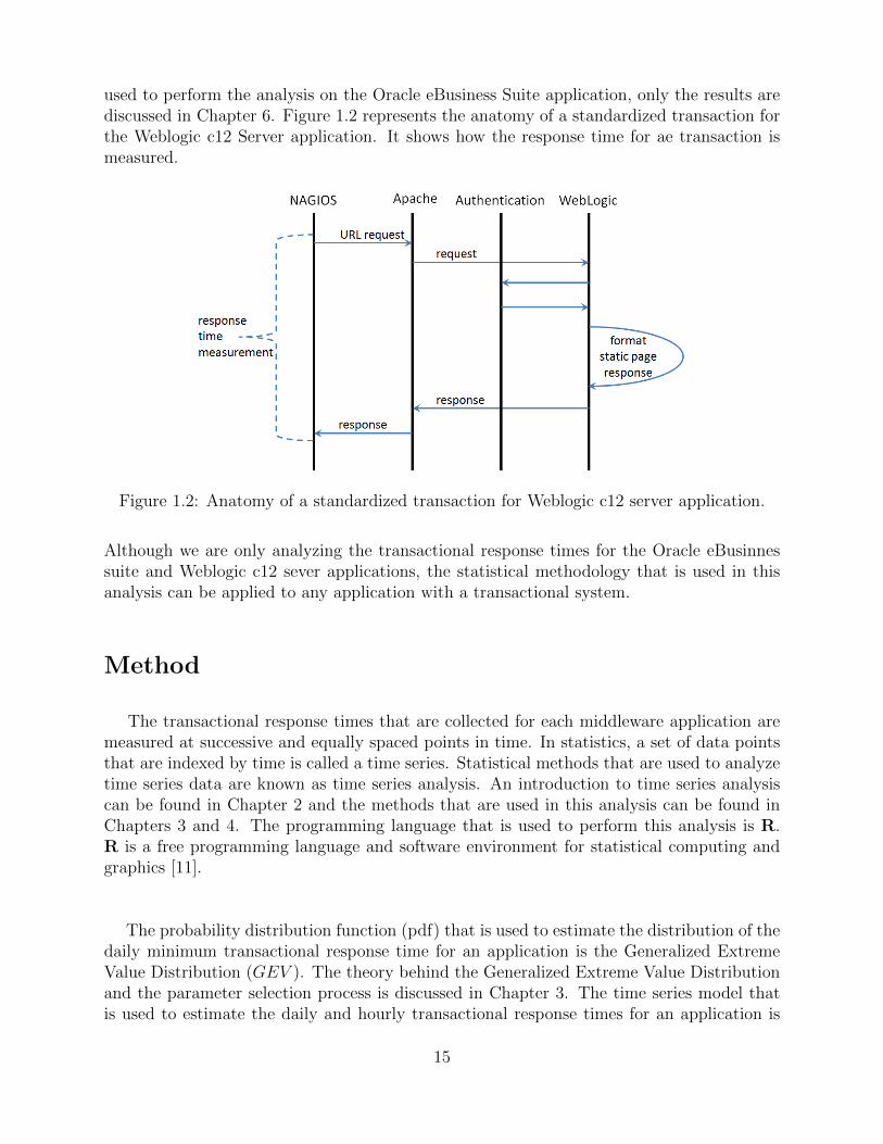
used to perform the analysis on the Oracle eBusiness Suite application, only the results arediscussed in Chapter 6. Figure 1.2 represents the anatomy of a standardized transaction forthe Weblogic c12 Server application. It shows how the response time for ae transaction ismeasured.

Figure 1.2: Anatomy of a standardized transaction for Weblogic c12 server application.

Although we are only analyzing the transactional response times for the Oracle eBusinnessuite and Weblogic c12 sever applications, the statistical methodology that is used in thisanalysis can be applied to any application with a transactional system.

Method

The transactional response times that are collected for each middleware application aremeasured at successive and equally spaced points in time. In statistics, a set of data pointsthat are indexed by time is called a time series. Statistical methods that are used to analyzetime series data are known as time series analysis. An introduction to time series analysiscan be found in Chapter 2 and the methods that are used in this analysis can be found inChapters 3 and 4. The programming language that is used to perform this analysis is R.R is a free programming language and software environment for statistical computing andgraphics [11].

The probability distribution function (pdf) that is used to estimate the distribution of thedaily minimum transactional response time for an application is the Generalized ExtremeValue Distribution (GEV ). The theory behind the Generalized Extreme Value Distributionand the parameter selection process is discussed in Chapter 3. The time series model thatis used to estimate the daily and hourly transactional response times for an application is

15

the Autoregressive Integrated Moving Average model (ARIMA). The theory behind thismodel and the selection of the model’s orders are discussed in Chapter 4. The results ofapplying these time series methods to the Oracle eBusiness Suite and Weblogic c12 Serverapplications are discussed in Chapters 5 and 6, respectively.

16

Chapter 2

Time Series

Introduction

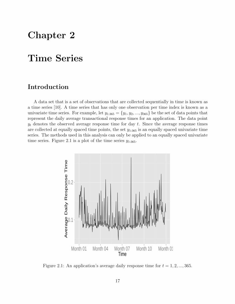
A data set that is a set of observations that are collected sequentially in time is known asa time series [10]. A time series that has only one observation per time index is known as aunivariate time series. For example, let y1:365 = y1, y2, ..., y365 be the set of data points thatrepresent the daily average transactional response times for an application. The data pointyt denotes the observed average response time for day t. Since the average response timesare collected at equally spaced time points, the set y1:365 is an equally spaced univariate timeseries. The methods used in this analysis can only be applied to an equally spaced univariatetime series. Figure 2.1 is a plot of the time series y1:365.

0.1

0.2

Month 01 Month 04 Month 07 Month 10 Month 01Time

Ave

rag

e D

aily R

esp

on

se

Tim

e

Figure 2.1: An application’s average daily response time for t = 1, 2, ..., 365.

17

In mathematics, a random variable is a variable whose value can take on any valuein it’s sample space. Each value in a random variable’s sample space is associated witha certain probability that is based on the random variable’s pdf. For example, let Y bethe random variable that represents the average daily transactional response time for anapplication and let Ω denote its sample space. Since response times are always greater than0, the sample space for Y is Ω = (0,+∞). If Y has a standard uniform distribution(Y ∼ uniform(a = 0, b = 1)), then all values in Ω have the equal probability of occurrence.Whereas, if Y is normally distributed with a mean equal to 2 and a variance equal to 1(Y ∼ normal(µ = 2, σ2 = 1)), the values in Ω that are close to 2 have a higher probabilityof occurring [2].

Let X be a random variable that has a pdf denoted by fX(x). The expected value of X,is the average value of X, weighted according to fX(x). It is denoted by E[X] and definedby

E[X] =

∫Ω

xfX(x)dx. (2.1)

The variance of X is the second central moment of X. It is denoted by V ar[X] and isdefined by

V ar[X] = E[(X − E[X])2]. (2.2)

The variance of a random variable can be interpreted as the measure of spread of its distri-bution around its mean [2].

A time series process is a set of random variables that are indexed by time and is denotedby

Y 1:T = Y 1,Y 2, ...,Y T.

A realization of a time series process is a set of observed values from a time series pro-cess. Since we have defined Y as the random variable that represents the average dailytransactional response time for an application, the time series plotted in Figure 2.1, y1:365 =y1, y2, ..., y365, is a realization of the time series process Y 1:365. For this analysis, a realiza-tion of time series processes will be referred to as a time series [10].

A random sample is a set of random variables that have a common probability distri-bution function, are independent and is denoted by X1:n = X1,X2, ..,Xn. Let x1:n =x1, x2, ..., xn be a realization, i.e. set of observed values, from the random sample X1:n.An important assumption when fitting observed data to a statistical model is that the datais a realization of independent random variables [2]. This assumption is always met when

18

analyzing x1:n because the random variables in X1:n are independent. However, this as-sumption is never met when analyzing a time series because the random variables in a timeseries process are indexed by time, making them dependent of each other [10].

For this analysis, random variables, random samples and time series process are denotedby a bold capital letter. Observed values are denoted by lower case letters. The sets ofletters (x,X) and (y,Y ) are used to differentiate between a random sample and a timeseries process. For example, X represents a random variable from a random sample and xrepresents an observation of a random sample. Whereas, Y represents a random variablefrom a time series process and y represents an observed value from a time series.

Stationarity

An important assumption made when fitting a time series to a statistical model is sta-tionarity. A time series is stationary if it is a realization of a stationary time series process.A time series process is stationary if there is a constant mean and variance throughout thewhole process and it’s behavior does not depend on when one starts to observe the process[10].

Stationarity in a Time Series Process

Two degrees of stationarity that are widely used in time series analysis are strong sta-tionarity and second order stationarity. It is very difficult to prove that a time series is arealization of a strong stationary time series process. Therefore, we will assume that a timeseries is stationary if we can prove that it is a realization of a time series process that issecond order stationary. A time series process, Y 1:T = Y 1, ...Y T, is said to be secondorder stationary if for any sequence of times, t1, .., tT , and any lag, h, all the first and secondjoint moments of (Y t1 , ...,Y tT )′ exists and are equal to the first and second moments of(Y t1+h, ...,Y tT+h)

′ [10]. In other words, a time series process, Y 1:T , is said to be secondorder stationary if

1. The expected value for all the random variables in Y1:T are equivalent: E[Y t] = µ forall t.

2. The variance for all the random variables in Y1:T are equivalent: V ar[Y t] = σ for allt [10].

19

Graphical Check of Stationarity

Two diagnostic plots that are used to check the assumption of stationarity in a time seriesare a time series plot and a autocorrelation function (ACF) plot. A time series plot is a plotof a realization of a time series process, i.e. a plot of an observed time series. A time seriesplot suggest non-stationarity if it contains graphical trend and/or seasonal pattern [10].

Figure 2.2 contains four time series plots. The times series in Figures 2.2(a) and 2.2(b)were generated in R. Figure 2.2(c) is a time series plot of the data set from the R Package fore-cast that contains Australia’s monthly gas production from 1956 to 1995 [6]. Figure 2.2(d)is a time series of the observations collected from an electroencephalogram corresponding toa patient undergoing ECT therapy [12].

Figure 2.2(a) suggest stationarity because there appears to be a constant mean andvariance throughout the observed period, whereas Figure 2.2(b) suggest non-stationarity withtrend because its mean increases over the observed period. Both Figures 2.2(c) and 2.2(d)suggest non-stationary with trend and seasonal pattern. The data points in each of theseplots form a sinusoidal pattern and increase/decrease over the observed period.

The ACF measures the linear dependence between two random variables from the sametime series process; one random variable at time t and one at time s. ACF is denoted byρ(t, s) and defined by [10]

ρ(t, s) =γ(t, s)√

var(Y t)var(Y s)(2.3)

where

γ(s, t) = Cov(Y t,Y s) = E(Y t − ut)(Y s − us)

ut = E[Y t]

us = E[Y s].

Note that the function γ(s, t) is the covariance function between random variables Yt and Ys.When dealing with data that is stationary, we may assume that E[Y t] = µ and V ar(Y t) = σ2

for all values of t. Therefore, for a stationary time series process, γ(t, s) only depends on thedistance between the indices t and s, |t − s| = h, making γ(s, t) = γ(h) = CovY t,Y t−hand ρ(t, s) = ρ(h) = γ(h)

γ(0). An ACF plot contains the values of the autocorrelation function

estimated from the time series. The ACF plot graphically explains the estimated correlationpatterns displayed by a time series process at different points in time [10].

20

0.0

0.1

0.2

0.3

0.4

0.5

0 25 50 75 100t

valu

e

(a) Stationary

0

10

20

30

0 100 200 300t

valu

e

(b) Non-Stationary w/ Trend

0

20000

40000

60000

1960 1970 1980 1990Date

Gas

Pro

duct

ion

(c) Non-Stationary w/ Trend and SeasonalCyclic Pattern

−200

−100

0

100

200

0 100 200 300 400 500t

EE

G

(d) Non-Stationary w/ Trend and SeasonalCyclic Pattern

Figure 2.2: Stationary vs. Non-Stationary Time Series Plots

Figure 2.3 contains the corresponding ACF plots for the time series plots in Figures 2.2.The blue dotted lines in the ACF plots represent the upper and lower confidence intervalsfor insignificant autocorrelations. A time series that is stationary produces an ACF plotthat contains values that are small and quickly approach zero as lag (h) increases. A timeseries that is non-stationary produces an ACF plot that contains values that are large, oftenpositive, that slowly or sometimes never approaches zero as h increases. The values tend tolie outside of the blue dotted lines [10].

21

0 5 10 15 20

−0.

20.

00.

20.

40.

60.

81.

0

Lag

AC

F

(a) Stationary

0 5 10 15 20 250.

00.

20.

40.

60.

81.

0

Lag

AC

F

(b) Non-Stationary w/ Trend

0.0 0.5 1.0 1.5 2.0

0.0

0.2

0.4

0.6

0.8

1.0

Lag

AC

F

(c) Non-Stationary w/ Trend and SeasonalPattern

0 5 10 15 20 25

−0.5

0.0

0.5

1.0

Lag

AC

F

(d) Non-Stationary w/ Trend and SeasonalPattern

Figure 2.3: Stationary vs. Non-Stationary ACF Plots

22

Algebraic Check of Stationarity

An algebraic method that is used to check the assumption of stationarity in a time seriesis the unit root test. The unit roots test that is used in this analysis is the Kwiatkowski-Phillips-Schmidt-Shin (KPSS) test. The KPPS test tests for either level-stationarity ortrend-stationarity. A time series process is level-stationary if it does not contain any un-derlying trend, whereas a time series process that is trend-stationary has underlying trendthat can be removed from the time series via smoothing operators. Since we are interestedin time series process that do not have any trend, we will use the level-stationarity KPSStest to test for stationarity. Thus, we will only explain the mathematics and structure of thelevel-stationary KPSS test in detail [8].

Let the time series y1:T be a realization of the time series process Y 1:T . In order to provethat y1:T is a stationary time series, the KPSS test is used to check if Y 1:T is a stationarytime series process. In order to perform the KPSS test, a linear stationary regression of Y t

on an intercept is fitted from the observed values in the time series y1:T . The regressionmodel is [8]

Y t = βo + εt (2.4)

for t = 1, 2, .., T

where

Y t = a random variable from Y 1:T that is indexed at time t

βo = intercept

εt = random variable that represents the stationary error at time t

where

εtiid∼ (0, σ2

ε).

The null hypothesis for this test assumes that the variance of the stationary error, denotedby σt, is equal to zero. The alternative hypothesis assumes that the variance of the stationaryerror is greater than zero:

Ho : σ2ε = 0 vs. Ha : σ2

ε > 0. (2.5)

The test statistic is denoted by ηµ and defined by [8]

23

ηµ = T−2

∑Tt = 1 (S2

t )

s2(l)(2.6)

where [8]

St =t∑i=1

ei (2.7)

s2(l) = T−1

T∑t = 1

(e2t ) + 2T−1

L∑s = 1

[(1 − s

L + 1)

T∑t = s+1

(etet − s)] (2.8)

L = o(T 1/2). (2.9)

The residual at time is the difference between the observed and fitted value at time t. It isdenoted by et and defined as

et = yt − yt. (2.10)

Note that yt is the fitted value, i.e. estimated value, at time t. This estimated valueis calculated from the fitted regression model, yt = βo. The fitted model only includes theestimated intercept βo. Therefore, et = yt− βo for all t. The estimated intercept is calculatedfrom the time series y1:T [8].

The upper tail critical values for ηµ can be found in Table 1 in Kwiatkowski et al. 1992.If ηµ is greater than the critical value at the α-level, then the null hypothesis is rejected at anα-level of significance and we may assume that y1:T is non-stationary. If ηµ is less than thecritical value at the α-level, then the null hypothesis is accepted at an α-level of significanceand we may assume that the time series y1:T is stationary [8].

It has already been shown graphically that the time series in Figure 2.2(a) is stationary.The KPSS test will be used to algebraically show that the time series in Figure 2.2(a) isstationary. The value of the test statistic that is calculated from this time series is ηµ =0.0390. In Kwiatkowski et al. 1992, Table 1 shows that at the α = .05 level of significance,the p-value for the given value of ηµ is .10. This implies that we do not have enough evidenceto reject the null hypothesis and that this time series has unit root. Therefore, the time seriesin Figure 2.2(a) has been shown to be graphically and algebraically stationary.

24

Removing Non-Stationarity

In time series analysis, the assumption of stationarity is important when modeling a timeseries. Because most time series are realizations of a non-stationary process, there existssmoothing techniques that are applied to time series in order to separate the non-stationarydata from the stationary data. These techniques involve decomposing the time series intoa “smooth” component and a component that contains the unexplained white noise. Twosmoothing techniques that are widely used and that are used in this analysis are movingaverages and differencing [10].

Suppose y1:T is a non-stationary time series. A technique that is used to remove thenon-stationarity from y1:T is by applying the moving average operator M , to y1:T . ApplyingM to y1:T returns the set of transformed values zq+1, zq+1, ..., zT−p where [10]

zt =

p∑j = −q

(ajyj + j), for t = (q + 1) : (T − p), (2.11)

where aj’s are weights that sum to one, aj ≥ 0 for all j and aj = a−j. It is generally assumedthat p = q, p and q are small values and an equal weight is selected for all j. The order of Mis equal to 2p+ 1 [10].

Figure 2.4 contains the results of applying the moving average operator with orders q = 3and q = 6 to the non-stationary time series in Figure 2.2. Figures 2.4(b) and 2.4(c) showthat the transformed values in the set zq+1, zq+1, ..., zT−p become smoother as the order ofthe moving average operator increases. The moving average smoothing technique removesthe white nose from the time series, but it does not remove the increasing trend.

25

Time

z

0 100 200 300

05

1015

2025

30

(a) Non-Stationary w/ Trend

Time

z

0 100 200 300

05

1015

2025

30

(b) Moving Average q = 3

Time

z

0 50 100 150 200 250 300 350

05

1015

2025

30

(c) Moving Average q = 6

Figure 2.4: Graphical results of applying the moving average operator to a non-stationarytime series with increasing trend

There exists two types of differencing techniques, non-seasonal differencing and seasonaldifferencing. Non-seasonal differencing is a smoothing technique that removes trend from atime series. The d-order non-seasonal differencing operator is denoted by Dd and defined by[9]

Dd = (1 − B)d. (2.12)

Dd is a function of the back-shift operator. The back-shift operator is denoted by B and isdefined by

Byt = yt−1. (2.13)

Applying the first-order non-seasonal differencing operator (D1) to the time series y1:T , re-

26

turns the set of transformed values z1, .., zT−1, where [9]

zt = D1yt = (1−B)1yt = yt − Byt = yt − yt−1 []. (2.14)

Time

z

0 100 200 300 400

010

000

2000

030

000

4000

050

000

6000

0

(a) Australian monthly gas productiontime series plot.

Time

z

0 100 200 300 400

−10

000

−50

000

5000

1000

0

(b) Time series plot of the D1 transformedvalues z1, .., zT−1.

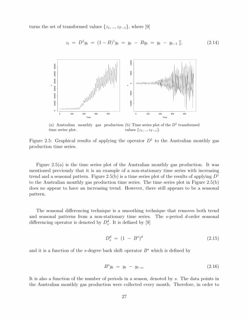
Figure 2.5: Graphical results of applying the operator D1 to the Australian monthly gasproduction time series.

Figure 2.5(a) is the time series plot of the Australian monthly gas production. It wasmentioned previously that it is an example of a non-stationary time series with increasingtrend and a seasonal pattern. Figure 2.5(b) is a time series plot of the results of applying D1

to the Australian monthly gas production time series. The time series plot in Figure 2.5(b)does no appear to have an increasing trend. However, there still appears to be a seasonalpattern.

The seasonal differencing technique is a smoothing technique that removes both trendand seasonal patterns from a non-stationary time series. The s-period d-order seasonaldifferencing operator is denoted by Dd

s . It is defined by [9]

Dds = (1 − Bs)d (2.15)

and it is a function of the s-degree back shift operator Bs which is defined by

Bsyt = yt − yt−s. (2.16)

It is also a function of the number of periods in a season, denoted by s. The data points inthe Australian monthly gas production were collected every month. Therefore, in order to

27

remove the seasonal pattern from the time series, the 12-period (monthly) first-order seasonaldifference operator, D1

12, is applied to the Australian gas production time series, y1:T . Thisreturns a vector of transformed values z1, .., zT−1 where [9]

zt = D112yt = (1−B12)1yt = yt −B12yt = yt − yt−12 [9]. (2.17)

Time

z

0 100 200 300 400

010

000

2000

030

000

4000

050

000

6000

0

(a) Australian monthly gas productiontime series plot.

Timez

0 100 200 300 400

−50

000

5000

1000

015

000

(b) Time series plot of the D112transformed

values z1, .., zT−1.

Figure 2.6: Graphical results of applying D112 to the Australian monthly gas production time

series.

Figure 2.6(b) is a time series plot that contains the results of applying D112 to the Australian

monthly gas production time series. There no longer appears to be an increasing trendnor seasonal pattern, implying that the D1

12 operator removed the non-stationarity from theAustralian monthly gas production time series.

28

Chapter 3

Extreme Values in a Time SeriesProcess

Extreme Value Theory - Stationary

Estimating the distribution of an event that occurs with very small probability is ofinterest in statistical inference. In statistics, these rare events are referred to as extremeevents and the theory of modeling and measuring these events is known as Extreme ValueTheory (EVT). Examples of statistics that are extreme events are maximums and minimums.Order Statistics is a statistical method that infers on the distributions of these extreme events[4].

Order Statistics

Let X1:n = X1,X2, ...,Xn be an random sample. The random variables in X1:n

placed in ascending order are known as the order statistics of X1:n. They are denoted byX(i:n) = X(1),X(2), ...,X(n) and they satisfy X(1) ≤ X(2) ≤ ... ≤ X(n). The orderstatistics are defined as

X(1) = minX1:n

X(2) = second smallestX1:n

.

.

.

X(n−1) = second largestX1:n

X(n) = maxX1:n.

Since order statistics are random variables, each order statistic has a unique pdf that iscalculated from the joint probability distribution of the random sample X1:n [2].

29

Let Z1:m = Z1, ..Zm be a set of independent random variables where fZi(zi) is thepdf for the random variable Zi. The joint probability distribution function of a set ofindependent random variables is equal to the product of each of the random variables’ pdfs.Therefore, the joint pdf for the set Z1:m is defined by [2]

fZ1,...,Zm(Z1, ...,Zm) =m∏i=1

fZi(zi) = fZ1(z1) ∗ ... ∗ fZm(zm). (3.1)

As mentioned previously, a random sample is a set of independent random variables thathave the same pdf. Therefore, the joint pdf of the random sample X1:n is defined by

fX1,...,Xn(x1, ..., xn) =n∏i=1

fX(x) = [fX(x)]n (3.2)

where fX(x) is the pdf for the random variables in X1:n [2]. Unlike a set of independentrandom variables or, more specifically, a random sample, the joint pdf of a set of randomvariables that are dependent is very difficult to calculate. Since the random variables in atime series process are dependent, the joint probability distribution of a time series processis almost impossible to calculate. Therefore, modeling the distribution of extreme values ina time series process can not be done through order statistics.

Generalized Extreme Value Distribution

Let Z1:n = Z1, , ...,Zn be a set of independent random variables. In Extreme ValueTheory, it has been shown that as n → ∞, the Generalized Extreme Value Distribution(GEV) is the limiting distribution of the order statistics Z(min) and Z(max) [4]. The GEV isa family of pdfs that combine the Gumbel, Frechet and Weibull distributions. The pdf forZ(max) is defined by [4]

fZ(max)(z|µ, σ, ξ) =

1

σt(z)ξ+1e−t(z) (3.3)

where

t(z) =

(1 + ( z−µ

σξ))

1ξ , if ξ 6= 0

e−z−µσ , if ξ = 0

(3.4)

and where

µ = location parameter

30

σ = scale parameter (> 0)

ξ = shape parameter.

The pdf for Z(min) is denoted by fZ(min)(z|µ, σ, ξ). Since it can be shown thatmin(Z1, ...,Zn) =

−max(−Z1, ...,−Zn), fZ(min)(z|µ, σ, ξ) is defined in terms of fZ(max)

(z|µ, σ, ξ) where

fZ(min)(Z|µ, σ, ξ) = 1− fZ(max)

(Z|µ, σ, ξ). (3.5)

Let X1:n be a random sample. Since a random sample is set of independent random vari-ables, for large values of n, the pdfs for X(min) and X(max) are denoted by fX(min)

(x|µ, σ, ξ)and fX(max)

(x|µ, σ, ξ) and are equivalent to equations 3.3 and 3.5, respectively,

fX(min)(x|µ, σ, ξ) = fZ(min)

(z|µ, σ, ξ) (3.6)

fX(max)(x|µ, σ, ξ) = fZ(max)

(z|µ, σ, ξ). (3.7)

Extreme Value Theorem for Stationary Time Series Processes

Let Y 1:n = Y 1, ..,Y n be a stationary time series process and let

Y (min) = minY 1, ...,Y n and Y (max) = minY 1, ...,Y n.

Unlike a random sample, the random variables in Y 1:n are neither independent nor identicallydistributed. Since neither of the assumptions of independence or an identical distributionare met, it would seem that the limiting distributions for Y (min) and Y (max) are not fromthe family of generalized extreme value distributions. However, the Extreme Value Theoremfor Stationary Time Series Process (EVTS) states that for large values of n, Y (min) andY (max) follow a GEV distribution when Y (min) and Y (max) are from a stationary time seriesprocess. In particular, the pdfs of Y (min) and Y (max) are denoted by fY (min)

(y|µ, σ, ξ) andfY (max)

(y|µ, σ, ξ), and are also equivalent to equations 3.3 and 3.5, respectively,

fY (min)(y|µ, σ, ξ) = fZ(min)

(z|µ, σ, ξ) (3.8)

fY (max)(y|µ, σ, ξ) = fZ(max)

(z|µ, σ, ξ). (3.9)

A full explanation and proof of the EVTS can be found in Haan et. al 2006.

31

The Block Minima/Maxima Method and the Peaks Over Threshold Method are twotechniques that are used to estimate the parameters in fY (min)

(y|µ, σ, ξ) and fY (max)(y|µ, σ, ξ).

Both of these techniques are based off of the EVTS. For this analysis, we will only explainthe Block Minima Method because it is used to estimate the distribution of an application’sminimum daily transactional response time.

Block Minima Method

Let y1:n be a time series from the stationary time series process Y 1:n. In extreme valuetheory, the block minima method consists of dividing the observation in y1:T into K non-overlapping blocks of equal size [3]. The set y(min)1:K = m1,m2, ...,mK consists of theobserved minimum values from each of the K blocks. The observations in y(min)1:K aredefined by

m1 = min(block 1)

m2 = min(block 2)

.

.

.

mk = min(block K).

In the EVTS, it has been proven that the limiting distribution of Y (min) (eqn. 3.8) can be

estimated by the pdf fY (min)(y|µ, σ, ξ), which is defined by

fY (min)(y|µ, σ, ξ) = 1− fY (max)

(−y|µ, σ, ξ) = 1− 1

σt(−y)ξ+1e−t(−y) (3.10)

where

t(−y) =

(1 + (−y−µ

σξ))

1

ξ , if ξ 6= 0

e−−y−µσ , if ξ = 0

and where

µ = estimated location parameter

σ = estimated scale parameter (> 0)

ξ = estimated shape parameter.

32

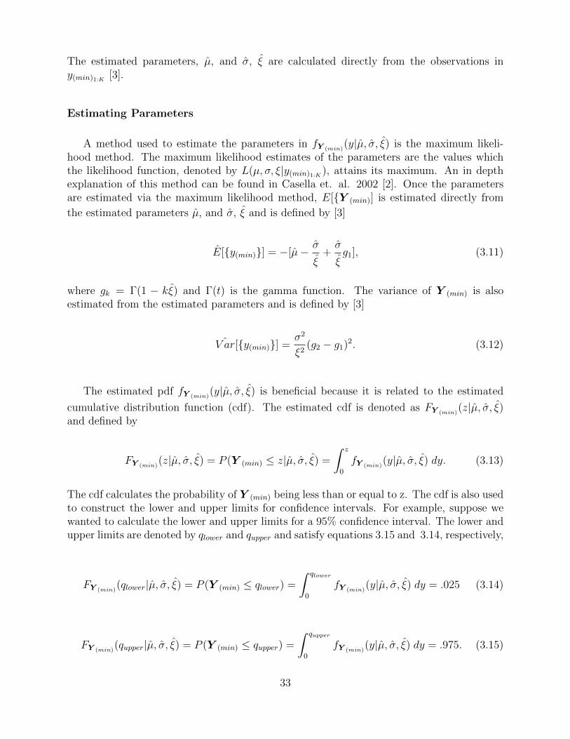
The estimated parameters, µ, and σ, ξ are calculated directly from the observations iny(min)1:K [3].

Estimating Parameters

A method used to estimate the parameters in fY (min)(y|µ, σ, ξ) is the maximum likeli-

hood method. The maximum likelihood estimates of the parameters are the values whichthe likelihood function, denoted by L(µ, σ, ξ|y(min)1:K ), attains its maximum. An in depthexplanation of this method can be found in Casella et. al. 2002 [2]. Once the parametersare estimated via the maximum likelihood method, E[Y (min)] is estimated directly from

the estimated parameters µ, and σ, ξ and is defined by [3]

E[y(min)] = −[µ− σ

ξ+σ

ξg1], (3.11)

where gk = Γ(1 − kξ) and Γ(t) is the gamma function. The variance of Y (min) is alsoestimated from the estimated parameters and is defined by [3]

ˆV ar[y(min)] =σ2

ξ2(g2 − g1)2. (3.12)

The estimated pdf fY (min)(y|µ, σ, ξ) is beneficial because it is related to the estimated

cumulative distribution function (cdf). The estimated cdf is denoted as FY (min)(z|µ, σ, ξ)

and defined by

FY (min)(z|µ, σ, ξ) = P (Y (min) ≤ z|µ, σ, ξ) =

∫ z

0

fY (min)(y|µ, σ, ξ) dy. (3.13)

The cdf calculates the probability of Y (min) being less than or equal to z. The cdf is also usedto construct the lower and upper limits for confidence intervals. For example, suppose wewanted to calculate the lower and upper limits for a 95% confidence interval. The lower andupper limits are denoted by qlower and qupper and satisfy equations 3.15 and 3.14, respectively,

FY (min)(qlower|µ, σ, ξ) = P (Y (min) ≤ qlower) =

∫ qlower

0

fY (min)(y|µ, σ, ξ) dy = .025 (3.14)

FY (min)(qupper|µ, σ, ξ) = P (Y (min) ≤ qupper) =

∫ qupper

0

fY (min)(y|µ, σ, ξ) dy = .975. (3.15)

33

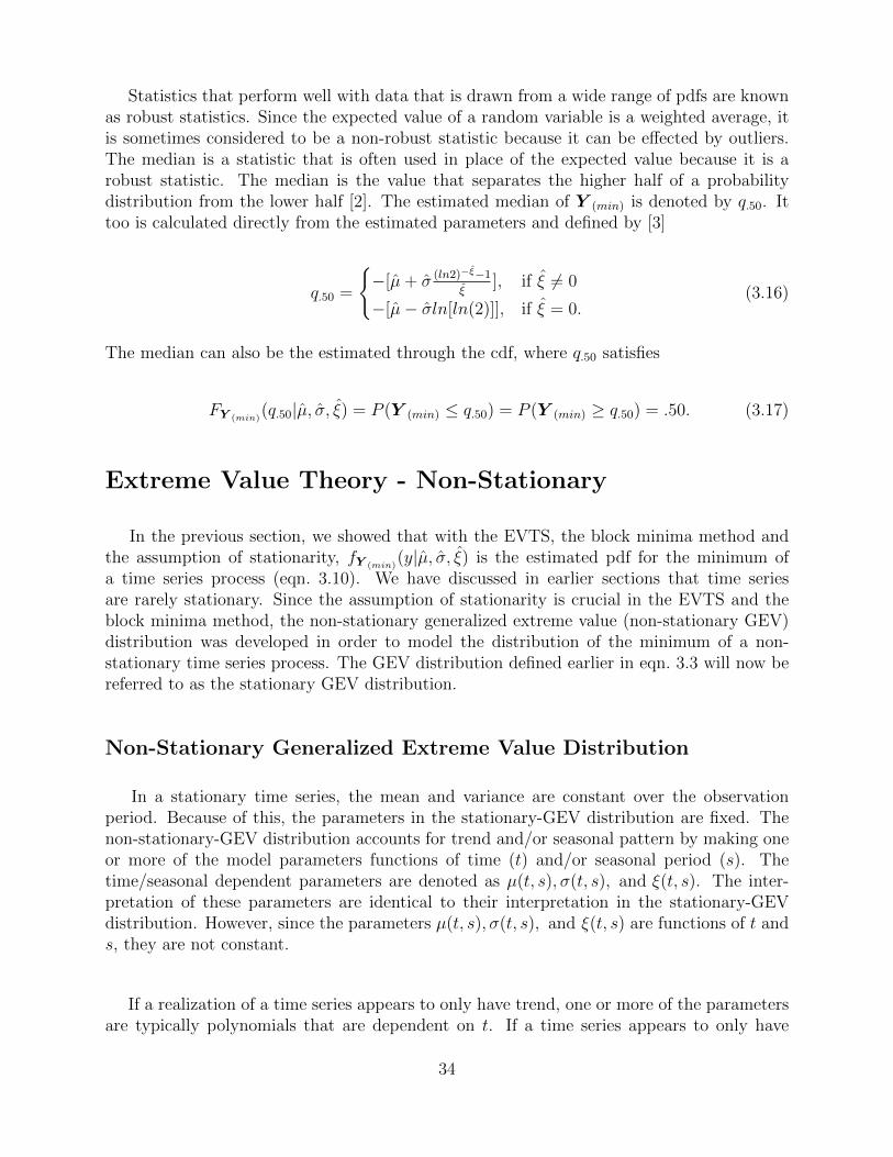
Statistics that perform well with data that is drawn from a wide range of pdfs are knownas robust statistics. Since the expected value of a random variable is a weighted average, itis sometimes considered to be a non-robust statistic because it can be effected by outliers.The median is a statistic that is often used in place of the expected value because it is arobust statistic. The median is the value that separates the higher half of a probabilitydistribution from the lower half [2]. The estimated median of Y (min) is denoted by q.50. Ittoo is calculated directly from the estimated parameters and defined by [3]

q.50 =

−[µ+ σ (ln2)−ξ−1

ξ], if ξ 6= 0

−[µ− σln[ln(2)]], if ξ = 0.(3.16)

The median can also be the estimated through the cdf, where q.50 satisfies

FY (min)(q.50|µ, σ, ξ) = P (Y (min) ≤ q.50) = P (Y (min) ≥ q.50) = .50. (3.17)

Extreme Value Theory - Non-Stationary

In the previous section, we showed that with the EVTS, the block minima method andthe assumption of stationarity, fY (min)

(y|µ, σ, ξ) is the estimated pdf for the minimum ofa time series process (eqn. 3.10). We have discussed in earlier sections that time seriesare rarely stationary. Since the assumption of stationarity is crucial in the EVTS and theblock minima method, the non-stationary generalized extreme value (non-stationary GEV)distribution was developed in order to model the distribution of the minimum of a non-stationary time series process. The GEV distribution defined earlier in eqn. 3.3 will now bereferred to as the stationary GEV distribution.

Non-Stationary Generalized Extreme Value Distribution

In a stationary time series, the mean and variance are constant over the observationperiod. Because of this, the parameters in the stationary-GEV distribution are fixed. Thenon-stationary-GEV distribution accounts for trend and/or seasonal pattern by making oneor more of the model parameters functions of time (t) and/or seasonal period (s). Thetime/seasonal dependent parameters are denoted as µ(t, s), σ(t, s), and ξ(t, s). The inter-pretation of these parameters are identical to their interpretation in the stationary-GEVdistribution. However, since the parameters µ(t, s), σ(t, s), and ξ(t, s) are functions of t ands, they are not constant.

If a realization of a time series appears to only have trend, one or more of the parametersare typically polynomials that are dependent on t. If a time series appears to only have

34

seasonal pattern, one or more of the parameters are typically sinusoidal functions that aredependent on s. If a time series appears to have trend and seasonal pattern, one or moreof the parameters are typically functions that are dependent on t and s. Table 3.1 containsthe structure of the three types of non-constant parameter functions.

Table 3.1: Time dependent parameter functions for the non-stationary GEV pdf.

Time (t) Seasonal (s) Time and Seasonal (t, s)

µ(t) = µo +∑pµ

k=1 µktk, µ(s) = µo + µsinsin(ωcs) + µcoscos(ωcs) µ(t, s) = µ(t) + µ(s)

σ(t) = σo +∑pσ

k=1 σktk σ(s) = σo + σsinsin(ωcs) + σcoscos(ωcs) σ(t, s) = σ(t) + σ(s)

ξ(t) = ξo +∑pξ

k=1 ξktk ξ(s) = ξo + ξsinsin(ωcs) + ξcoscos(ωcs) ξ(t, s) = ξ(t) + ξ(s)

Note: The set of parameters pµ, pσ, pξ represents the degrees of their correspondingpolynomial functions. The sets of parameters θµ = µo, µ1, ..., µpµ , µsin, µcos, θσ =σo, σ1, ..., σpσ , σsin, σcos and θξ = ξo, ξ1, ..., ξpξ , ξsin, ξcos are the coefficients for their corre-sponding functions. The parameter ω = 2π

365.25and the variable cs denotes the center of the

s-th period counted in days starting from the beginning of the year.

Model Selection

Let y1:T be a time series that is a realization of the time series process Y 1:T . Supposewe are interested in estimating the parameters in fY (min)

(y|µ, σ, ξ) from the time series y1:T .The first step in estimating the the parameters is determining if y1:T is stationary. Thestationarity of a time series is visually analyzed through the time series and ACF plots ofy1:T . The stationarity of y1:T is then analyzed algebraically with the KPSS unit root test.

If the results of these plots and test suggest that y1:T is a stationary time series, then theblock minima method is implemented and the parameters for the stationary-GEV distribu-tion are estimated from the set of block minimums y(min)1:K . However, if the results suggestthat y1:T is a non-stationary time series, then the block minima method is still implementedbut the parameters for the non-stationary GEV distribution are estimated from y(min)1:K .

35

In R, there exists functions that only estimate the parameters in fY (max)(y|µ, σ, ξ). There-

fore, a problem arises in R when estimating the parameters in fY (min)(y|µ, σ, ξ). Equa-

tion 3.10 states that fY (min)(y|µ, σ, ξ) is defined as

fY (min)(y|µ, σ, ξ) = 1− fY (max)

(y|µ, σ, ξ).

Therefore, fitting the negative of the block minimums (−y(min)1:K ) to fY (max)(y|µ, σ, ξ) would

avoid this problem in R. However, the functions in R that would be used to perform this fithave a difficult time handling data with negative values.

It can be proven that 1min(Y 1,...,Y n)

= max( 1Y 1, ..., 1

Y n). Therefore, the following transfor-

mation and analysis will be performed in R to to estimate the mean, median and confidencebands for Y(min):

1. Perform a normalized reciprocal transformation on the set of block minimums (y(min)1:K ).The purpose of normalizing the data is that it returns a better fit and a lower AIC value.The set of the transformed block minimums is denoted as z(min)1:K = z1, z2, .., zK.The transformed minimum for block k is denoted as zk and defined by

zk =1mk− µrecipvrecip

(3.18)

where

mk = min(blockk)

µrecip = 1K

∑Kk=1

1mk

vrecip = 1K

∑Kk=1( 1

mk− µrecip)2.

2. Fit the transformed values z(min)1:K = z1, z2, .., zK to fY (max)(y|µ, σ, ξ) in R with the

function gev.fit from the ismev package [5].

3. Once the estimated parameters are calculated, the estimated expected value and me-dian of Y(min) are calculated from the following two equations:

E[y(min)] = [µ− σ

ξ+σ

ξg1] ∗ vrecip + µrecip, (3.19)

q.50 =

[µ+ σ (ln2)−ξ−1

ξ] ∗ vrecip + µrecip, if ξ 6= 0

[µ− σln[ln(2)]] ∗ vrecip + µrecip, if ξ = 0.(3.20)

36

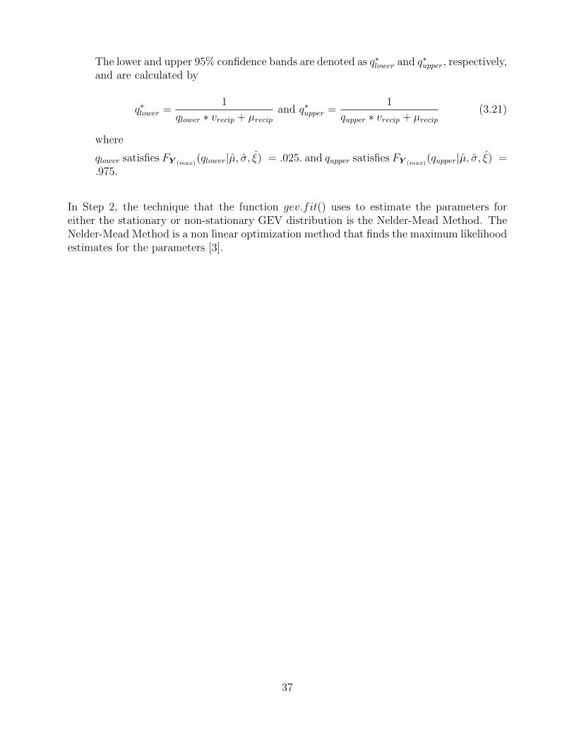
The lower and upper 95% confidence bands are denoted as q∗lower and q∗upper, respectively,and are calculated by

q∗lower =1

qlower ∗ vrecip + µrecipand q∗upper =

1

qupper ∗ vrecip + µrecip(3.21)

where

qlower satisfies FY (max)(qlower|µ, σ, ξ) = .025. and qupper satisfies FY (max)

(qupper|µ, σ, ξ) =.975.

In Step 2, the technique that the function gev.fit() uses to estimate the parameters foreither the stationary or non-stationary GEV distribution is the Nelder-Mead Method. TheNelder-Mead Method is a non linear optimization method that finds the maximum likelihoodestimates for the parameters [3].

37

38

Chapter 4

Modeling Time Series

Introduction

In order to understand the relationship between the sequential observations in a time seriesand be able to forecast future observations, time series are fitted to statistical models. Forexample, recall the time series, y1:365, that is plotted in Figure 2.1 contains an application’sdaily average response times. Questions that may arise when analyzing this time series ishow a day’s average response time is related to the previous days’ average response timesor if the day of the week or month has influence on a day’s average response time. Fittingy1:365 to an appropriate statistical model will provide answers to these questions.

There are different types of statistical models that can be used to analyze a time series.The selection of the model often depends on the stationarity of the time series. If a timeseries is stationary, either an autoregressive, a moving average, or an autoregressive movingaverage model can be selected as the most appropriate model. If the time series is non-stationary, a mixed model that incorporates smoothing techniques is often selected as themost appropriate model. Two non-stationary mixed models that are discussed in this analysisare the seasonal and non-seasonal autoregressive integrated moving average models. Again,the selection of the most appropriate mixed model depends on the type of non-stationaritythat is present in the time series.

Non-Mixed Models

Autoregressive Model: AR(p)

If the time series y1:365 is a realization of the stationary time series process that assumes aday’s average response time is dependent only on the previous days’ average response times,then an autoregressive model with order p (Ar(p)) would be used to model the dependenciesin y1:365. The AR(p) model is the simplest time series model that is used to explore thedependencies between random variables in a stationary time series process. The order of an

39

autoregressive time series model is denoted by p and it represents the maximum distance(|t− s|) between random variables Yt and Ys such that cov(Yt,Ys) is significant [10].

The time series process Y1:T is an Ar(p) process if each Yt arises from the autoregressivetime series model [10]

Yt =

p∑j=1

φjYt−j + εt (4.1)

where

p = model order

φj = model parameter for Yt−j

εt = stationary error at time t.

It is often assumed that for all t, εtiid∼ normal(0, v). Suppose Yt arises from an autoregressive

time series process with order p = 3. This implies that the value of Yt depends on Yt−1,Yt−2

and Yt−3 and the stationary error at time t and is equivalent to

Yt =3∑j=1

φjYt−j + εt,= φ1Yt−1 + φ2Yt−2 + φ3Yt−3 + εt.

The autoregressive characteristic polynomial of an AR(p) process is denoted as Φ anddefined by [10]

Φ = 1−p∑j=1

φjuj [10]. (4.2)

If Φ(u) = 0 only for values of u such that |u| < 1, then the autoregressive characteristicpolynomial, Φ, has unit root. Causality is the direct cause and effect relationship betweentwo observations. An AR(p) process is casual if Φ has unit root. Causality of an AR(p)process implies stationarity, however, stationarity does not imply causality [10].

When fitting y1:T to an AR(p) model, the set of model parameters φ = φ1.φ2, ..., φpare estimated directly from y1:T . The set of estimated parameters are denoted by φ= φ1, φ2, ..., φp. The most common technique that is used to estimate the parametersin a statistical model is the maximum likelihood method [10]. The maximum likelihood

40

estimates of the parameters φ, are the values which the likelihood function, denoted byL[φ|y1:T )], attains its maximum [2].

The appropriate order of an AR(p) model is chosen via the Akaike Information Criterion(AIC) method. The AIC method involves fitting y1:T to AR models for different values of p.The value of p that returns the fitted AR model with the lowest AIC value is then selectedas the most appropriate model. The equation for AIC is [10]

AIC = 2k − 2ln(L) (4.3)

where

k = number of parameters in the model

L = L[φ|y1:T )].

Once φ are estimated and p is selected, the fitted values of y1:T , denoted by y1:T , areestimated from the fitted AR(p) model

yt =

p∑j=1

φj yt−j (4.4)

where

y1 = y1, y2 = y2, ..., yp = yp.

Moving Average Model: MA(q)

If the time series y1:365 is a realization of the stationary time series process that assumes aday’s average response time is dependent only on the previous days’ average response times’random errors, then a moving average time series model with order q (MA(q)) would be usedto model the dependencies in y1:365. The MA(q) model is used to model the random errordependencies in a time series process. The parameter q represents the order of a movingaverage model and it is defined as the maximum distance (|t − s|) between the randomvariables Yt and Ys such that cov(εt,εs) is significant [10].

The time series process Y1:T is an MA(q) process if each Yt arises from the movingaverage time series model [10]

41

Yt =

q∑j=1

θjεt−j + εt, (4.5)

where

q = model order

θj = model parameters for εt−j

εt = stationary error at time t.

It is often assumed that εtiid∼ normal(0, v). The moving average characteristic polynomial

of an MA(q) process is denoted by Θ and defined by [10]

Θ = 1−q∑j=1

θjuj. (4.6)

If Θ(u) = 0 only for |u| < 1, then Θ has unit root. An important assumption for a MA(q)process is that the parameters θ are identifiable. An MA(q) process is identifiable if Θhas unit root [10].

The MA(q) model parameters φ = θ1.θ2, ..., θq are estimated via the method of

maximum likelihood and they are denoted as θ = θ1, θ2, ..., θq. The appropriate value of

q is chosen via the AIC method. Once θ are estimated and p is selected, the fitted values,denoted by y1:T , are estimated from the fitted model

yt =

q∑j=1

θj εj−q (4.7)

where

εt = yt − yj−q for t = p+ 1, ..., T

ε1, ε2, ..., εpiid∼ normal(0, v) [10] .

Forecast Function

Suppose we fit y1:365 to an AR(p) model. Once the value of p is selected and the modelparameters are estimated, the fitted values are calculated directly from equation 4.4. Thefitted values, denoted by y1:365, represent the estimated daily average transactional response

42

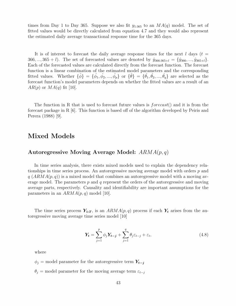
times from Day 1 to Day 365. Suppose we also fit y1:365 to an MA(q) model. The set offitted values would be directly calculated from equation 4.7 and they would also representthe estimated daily average transactional response time for the 365 days.

It is of interest to forecast the daily average response times for the next l days (t =366, ..., 365 + l). The set of forecasted values are denoted by y366:365+l = y366, ..., y365+l.Each of the forecasted values are calculated directly from the forecast function. The forecastfunction is a linear combination of the estimated model parameters and the correspondingfitted values. Whether φ = φ1, φ2, ..., φp or θ = θ1, θ2, ..., θq are selected as theforecast function’s model parameters depends on whether the fitted values are a result of anAR(p) or MA(q) fit [10].

The function in R that is used to forecast future values is forecast() and it is from theforecast package in R [6]. This function is based off of the algorithm developed by Peiris andPerera (1988) [9].

Mixed Models

Autoregressive Moving Average Model: ARMA(p, q)

In time series analysis, there exists mixed models used to explain the dependency rela-tionships in time series process. An autoregressive moving average model with orders p andq (ARMA(p, q)) is a mixed model that combines an autoregressive model with a moving av-erage model. The parameters p and q represent the orders of the autoregressive and movingaverage parts, respectively. Causality and identifiability are important assumptions for theparameters in an ARMA(p, q) model [10].

The time series process Y1:T , is an ARMA(p, q) process if each Yt arises from the au-toregressive moving average time series model [10]

Yt =

p∑j=1

φjYt−j +

q∑j=1

θjεt−j + εt, (4.8)

where

φj = model parameter for the autoregressive term Yt−j

θj = model parameter for the moving average term εt−j

43

εt = stationary error at time t.

The autoregressive moving average time series model can also be written in terms of thecharacteristic equations 4.2 and 4.6 and the back shift operator B (eqn. 2.13) [10]

Φ(B)Yt = Θ(B)εt (4.9)

where

Φ(B) = (1− φ1B1 − ...− φpBp) and Θ(z) = (1− θ1B

1 − ...− θpBq). (4.10)

Autoregressive Integrated Moving Average Model: ARIMA

As mentioned before, causality and identifiability are important assumptions when fittinga time series to either an AR(p), MA(q) or ARMA(p, q) model. If a time series is non-stationary, these assumptions are rarely met. Since it is frequent that time series processes arenon-stationary with trends and seasonal patterns, there exists an autoregressive integratedmoving average model (ARIMA) that is used to analyze the dependency within a non-stationary time series process. There exists two types of ARIMA models; a non-seasonalautoregressive integrated moving average model with orders p, q and d (ARIMA(p, q, d))and a seasonal autoregressive integrated moving average model with orders p, q, d, P , Q, D,and s (ARIMA(p, q, d)(P,Q,D)[s]) [7].

Non-Seasonal ARIMA(p, q, d) Model

If the observed daily average response times from y1:365 increased over the 365 day period,we would assume that y1:365 is a realization of a time series process that is non-stationarywith increasing trend. The non-seasonal ARIMA(p, q, d) model is appropriate for modelinga time series that appears to be non-stationary with trend. The ARIMA(p, q, d) differs fromthe ARMA(p, q) in that the prior applies the non-seasonal differencing operator to the timeseries in order to remove non-stationary trend [7].

The time series process Y1:t is a non-seasonal ARIMA(p, q, d) process if each Yt arisesfrom the autoregressive integrated moving average time series model [7]

Φ(B)DdYt = Θ(B)εt (4.11)

where

εt = stationary error at time t.

44

Dd = non-seasonal differencing technique defined in equation 2.12.

It is assumed that the εt’s are independent and identically distributed with mean zero andvariance equal to v. The functions Φ and Θ are the characteristic function of the autore-gressive and moving average parts defined in equation 4.10 [7].

Seasonal ARIMA(p, q, d)[P,D,Q][s] Model

If the values of observed daily average response times from y1:365 depended on the monththey were observed, we would assume that y1:365 is a realization of a time series process thatis non-stationary with trend and seasonal pattern. The seasonal ARIMA(p, q, d)(P,D,Q)[s]

model is appropriate for modeling a time series that appears to be non-stationary with trendand seasonal pattern with period s. The ARIMA(p, q, d)(P,D,Q)[s] applies a combinationof the non-seasonal and seasonal differencing operators to the time series in order to removethe non-stationarity and explain the dependencies that exits due to the seasonal patterns[7].

The time series process Y1:T is a seasonal ARIMA(p, q, d)(P,D,Q)[s] process if each Yt

arises from the autoregressive integrated moving average time series model [7]

Φ(Bs)Φ(B)DDs D

dYt = Θ(Bs)Θ(B)εt, (4.12)

where

εt = stationary error at time t.

Dsd = seasonal differencing operator defined in equation 2.15.

It is assumed that the εt’s are independent and identically distributed with mean zeroand variance equal to v. The functions Φ(B) and Θ(B) are defined in equation 4.10. The

functions Φ and Θ are the seasonal characteristic functions for the autoregressive and movingparts with degree P and Q, respectively, and they are defined by [7]

Φ(Bs) = [1− Φ1(Bs)1 − ...− Φp(Bs)P ] and Θ(z) = [1− Θ1(Bs)1 − ...− Θp(B

s)Q]. (4.13)

45

Model Selection

Saturated Model.

Let M denote a set of models that are being analyzed in a time series model selection.Determining which model in M is the most appropriate to model the dependency relation-ships in a time series is a difficult task. There exists a hierarchy of models in M and thesaturated model is the ”largest model” because it can explain all other models in M . Allother models in M can be written in terms of the saturated model because they are reducedversions of the saturated model. Before selecting a model, it is important to test all reducedmodels in M against the saturated model in M .

Let M be the set of the time series models previously discussed

M = AR(p), MA(q), ARMA(p, q), ARIMA(p, d, q), ARIMA(p, q, d)(P,D,Q)[s].

The saturated model in M is the seasonal ARIMA(p, q, d)(P,D,Q)[s] model because everyreduced model in M can be written in terms of the seasonal ARIMA model (Eq. 4.12). Forexample, suppose Yt arises from the seasonal ARIMA process with P = Q = D = 0 and s =1, ARIMA(p, q, d)(0, 0, 0)[1]. Yt is written as

Φ(B1)Φ(B)D01D

dYt = Θ(B1)Θ(B)εt

⇒ Φ(B1)Φ(B)(1−B1)0DdYt = Θ(B1)Θ(B)εt

⇒ Φ(B1)Φ(B)DdYt = Θ(B1)Θ(B)εt.

Since Φ and Θ are polynomials of order P = 0 and Q = 0, Φ(B1) = Θ(B1) = 1. Therefore,Yt arises from

Φ(B)DdYt = Θ(B)εt. (4.14)

Since equation 4.14 is equivalent to equation 4.11, Yt arises from the non-seasonalARIMA(p, d, q)process, implying that ARIMA(p, q, d)(0, 0, 0)[1] = ARIMA(p, q, d).

46

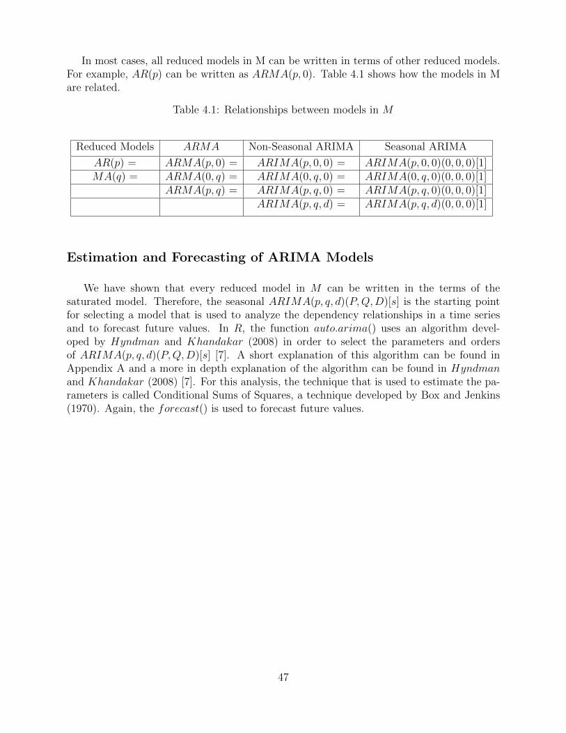
In most cases, all reduced models in M can be written in terms of other reduced models.For example, AR(p) can be written as ARMA(p, 0). Table 4.1 shows how the models in Mare related.

Table 4.1: Relationships between models in M

Reduced Models ARMA Non-Seasonal ARIMA Seasonal ARIMA

AR(p) = ARMA(p, 0) = ARIMA(p, 0, 0) = ARIMA(p, 0, 0)(0, 0, 0)[1]MA(q) = ARMA(0, q) = ARIMA(0, q, 0) = ARIMA(0, q, 0)(0, 0, 0)[1]

ARMA(p, q) = ARIMA(p, q, 0) = ARIMA(p, q, 0)(0, 0, 0)[1]ARIMA(p, q, d) = ARIMA(p, q, d)(0, 0, 0)[1]

Estimation and Forecasting of ARIMA Models

We have shown that every reduced model in M can be written in the terms of thesaturated model. Therefore, the seasonal ARIMA(p, q, d)(P,Q,D)[s] is the starting pointfor selecting a model that is used to analyze the dependency relationships in a time seriesand to forecast future values. In R, the function auto.arima() uses an algorithm devel-oped by Hyndman and Khandakar (2008) in order to select the parameters and ordersof ARIMA(p, q, d)(P,Q,D)[s] [7]. A short explanation of this algorithm can be found inAppendix A and a more in depth explanation of the algorithm can be found in Hyndmanand Khandakar (2008) [7]. For this analysis, the technique that is used to estimate the pa-rameters is called Conditional Sums of Squares, a technique developed by Box and Jenkins(1970). Again, the forecast() is used to forecast future values.

47

48

Chapter 5

Implementation To Oracle eBusinessSuite Application

Introduction

A transactional test is performed every five minutes on the Oracle eBusiness Suite appli-cation in order to monitor the application’s transactional response time. These tests measurethe amount of time it takes the application to receive a request and return a result. Thesemeasurements are stored in Nagios. Nagios is an open source network monitoring softwareapplication. A script was created in order to extract the data for this analysis from Nagios.

The transactional response times that were recorded over a 386 day period are used forthis analysis. Each recording contains two elements; an unformatted time stamp (GMT timezone) and its corresponding transactional response time (seconds). The recordings observedfrom Day 1 to Day 365 make up Data Set 1 and are used to estimate the parameters of theGEV distribution and ARIMA model. The recordings observed from Day 366 to Day 386are used to test the accuracy of these estimations.

Daily Minimum Transactional Response Time

Checking for Stationarity

In order to determine whether a stationary GEV or a non-stationary GEV distributionwill be used to estimate the distribution of the minimum transactional response time for theOracle eBusiness Suite application, the assumption of stationary is investigated in Data Set1.

Figure 5.1 contains the time series and ACF plots of the transactional response timesobserved from Day 1 to Day 365 (Data Set 1). In Figure 5.1(a), the response times appear

49

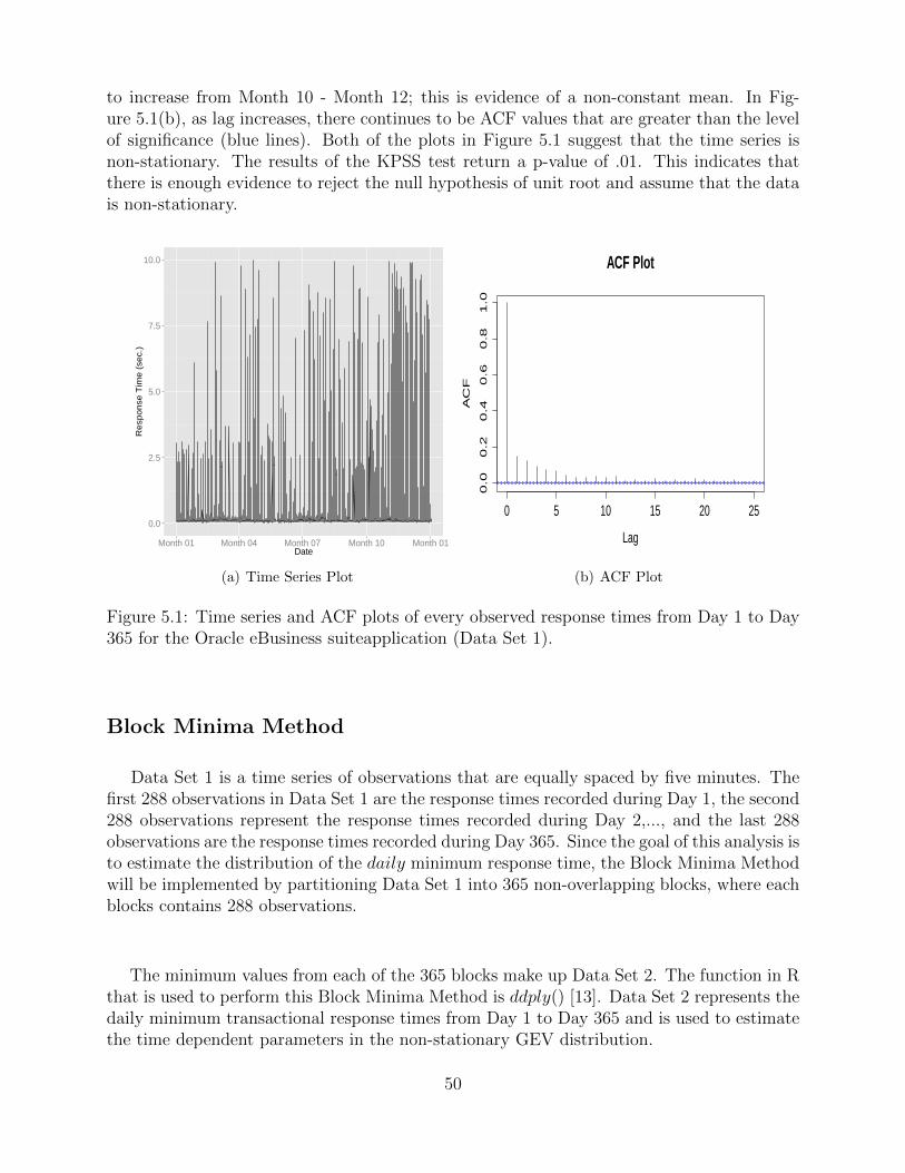
to increase from Month 10 - Month 12; this is evidence of a non-constant mean. In Fig-ure 5.1(b), as lag increases, there continues to be ACF values that are greater than the levelof significance (blue lines). Both of the plots in Figure 5.1 suggest that the time series isnon-stationary. The results of the KPSS test return a p-value of .01. This indicates thatthere is enough evidence to reject the null hypothesis of unit root and assume that the datais non-stationary.

0.0

2.5

5.0

7.5

10.0

Month 01 Month 04 Month 07 Month 10 Month 01Date

Re

spo

nse

Tim

e (

sec.

)

(a) Time Series Plot

0 5 10 15 20 25

0.0

0.2

0.4

0.6

0.8

1.0

Lag

AC

F

ACF Plot

(b) ACF Plot

Figure 5.1: Time series and ACF plots of every observed response times from Day 1 to Day365 for the Oracle eBusiness suiteapplication (Data Set 1).

Block Minima Method

Data Set 1 is a time series of observations that are equally spaced by five minutes. Thefirst 288 observations in Data Set 1 are the response times recorded during Day 1, the second288 observations represent the response times recorded during Day 2,..., and the last 288observations are the response times recorded during Day 365. Since the goal of this analysis isto estimate the distribution of the daily minimum response time, the Block Minima Methodwill be implemented by partitioning Data Set 1 into 365 non-overlapping blocks, where eachblocks contains 288 observations.

The minimum values from each of the 365 blocks make up Data Set 2. The function in Rthat is used to perform this Block Minima Method is ddply() [13]. Data Set 2 represents thedaily minimum transactional response times from Day 1 to Day 365 and is used to estimatethe time dependent parameters in the non-stationary GEV distribution.

50

Selection of Time Dependent Parameters

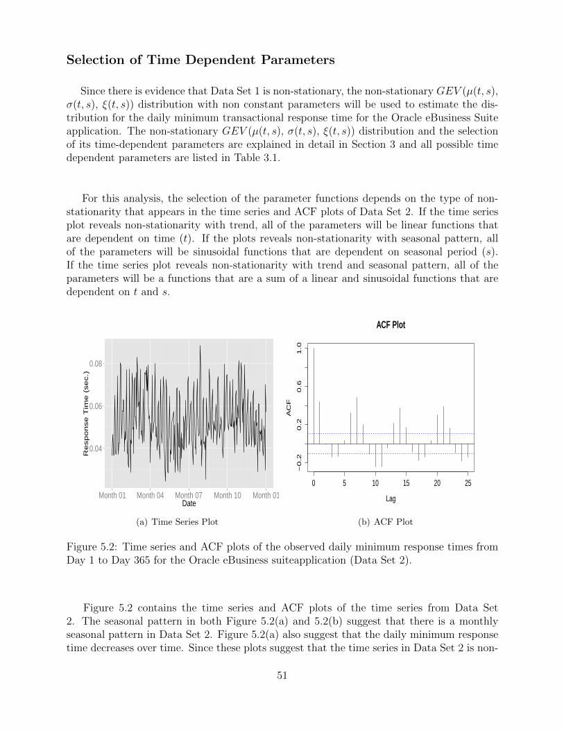
Since there is evidence that Data Set 1 is non-stationary, the non-stationary GEV (µ(t, s),σ(t, s), ξ(t, s)) distribution with non constant parameters will be used to estimate the dis-tribution for the daily minimum transactional response time for the Oracle eBusiness Suiteapplication. The non-stationary GEV (µ(t, s), σ(t, s), ξ(t, s)) distribution and the selectionof its time-dependent parameters are explained in detail in Section 3 and all possible timedependent parameters are listed in Table 3.1.

For this analysis, the selection of the parameter functions depends on the type of non-stationarity that appears in the time series and ACF plots of Data Set 2. If the time seriesplot reveals non-stationarity with trend, all of the parameters will be linear functions thatare dependent on time (t). If the plots reveals non-stationarity with seasonal pattern, allof the parameters will be sinusoidal functions that are dependent on seasonal period (s).If the time series plot reveals non-stationarity with trend and seasonal pattern, all of theparameters will be a functions that are a sum of a linear and sinusoidal functions that aredependent on t and s.

0.04

0.06

0.08

Month 01 Month 04 Month 07 Month 10 Month 01Date

Re

sp

on

se

Tim

e (

se

c.)

(a) Time Series Plot

0 5 10 15 20 25

−0

.20

.20

.61

.0

Lag

AC

F

ACF Plot

(b) ACF Plot

Figure 5.2: Time series and ACF plots of the observed daily minimum response times fromDay 1 to Day 365 for the Oracle eBusiness suiteapplication (Data Set 2).

Figure 5.2 contains the time series and ACF plots of the time series from Data Set2. The seasonal pattern in both Figure 5.2(a) and 5.2(b) suggest that there is a monthlyseasonal pattern in Data Set 2. Figure 5.2(a) also suggest that the daily minimum responsetime decreases over time. Since these plots suggest that the time series in Data Set 2 is non-

51

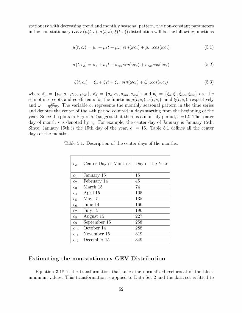
stationary with decreasing trend and monthly seasonal pattern, the non-constant parametersin the non-stationary GEV (µ(t, s), σ(t, s), ξ(t, s)) distribution will be the following functions

µ(t, cs) = µo + µ1t+ µsinsin(ωcs) + µcoscos(ωcs) (5.1)

σ(t, cs) = σo + σ1t+ σsinsin(ωcs) + σcoscos(ωcs) (5.2)

ξ(t, cs) = ξo + ξ1t+ ξsinsin(ωcs) + ξcoscos(ωcs) (5.3)

where θµ = µo, µ1, µsin, µcos, θσ = σo, σ1, σsin, σcos, and θξ = ξo, ξ1, ξsin, ξcos are thesets of intercepts and coefficients for the functions µ(t, cs), σ(t, cs), and ξ(t, cs), respectivelyand ω = 2π

365.25. The variable cs represents the monthly seasonal pattern in the time series

and denotes the center of the s-th period counted in days starting from the beginning of theyear. Since the plots in Figure 5.2 suggest that there is a monthly period, s =12. The centerday of month s is denoted by cs. For example, the center day of January is January 15th.Since, January 15th is the 15th day of the year, c1 = 15. Table 5.1 defines all the centerdays of the months.

Table 5.1: Description of the center days of the months.

cs Center Day of Month s Day of the Year

c1 January 15 15c2 February 14 45c3 March 15 74c4 April 15 105c5 May 15 135c6 June 14 166c7 July 15 196c8 August 15 227c9 September 15 258c10 October 14 288c11 November 15 319c12 December 15 349

Estimating the non-stationary GEV Distribution

Equation 3.18 is the transformation that takes the normalized reciprocal of the blockminimum values. This transformation is applied to Data Set 2 and the data set is fitted to

52

the non-stationary GEV distribution in R via the function gev.fit(). Appropriate residualdiagnostics were performed and the data appears to fit the distribution appropriately.

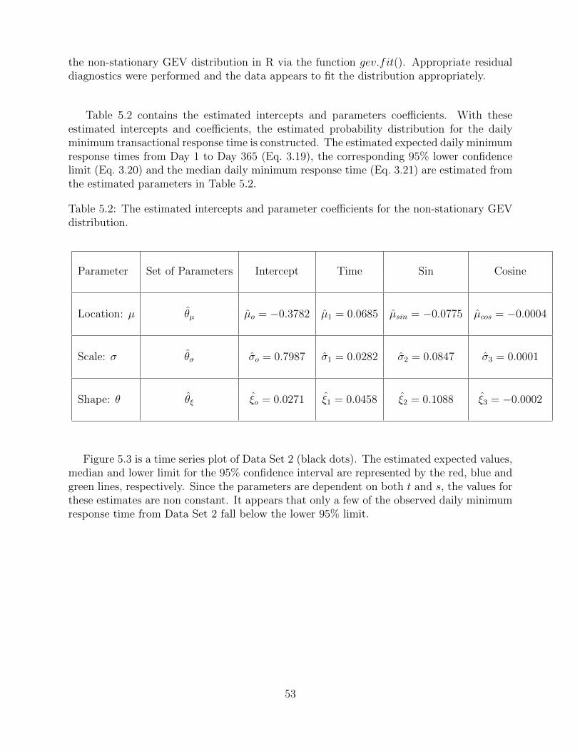
Table 5.2 contains the estimated intercepts and parameters coefficients. With theseestimated intercepts and coefficients, the estimated probability distribution for the dailyminimum transactional response time is constructed. The estimated expected daily minimumresponse times from Day 1 to Day 365 (Eq. 3.19), the corresponding 95% lower confidencelimit (Eq. 3.20) and the median daily minimum response time (Eq. 3.21) are estimated fromthe estimated parameters in Table 5.2.

Table 5.2: The estimated intercepts and parameter coefficients for the non-stationary GEVdistribution.

Parameter Set of Parameters Intercept Time Sin Cosine

Location: µ θµ µo = −0.3782 µ1 = 0.0685 µsin = −0.0775 µcos = −0.0004

Scale: σ θσ σo = 0.7987 σ1 = 0.0282 σ2 = 0.0847 σ3 = 0.0001

Shape: θ θξ ξo = 0.0271 ξ1 = 0.0458 ξ2 = 0.1088 ξ3 = −0.0002

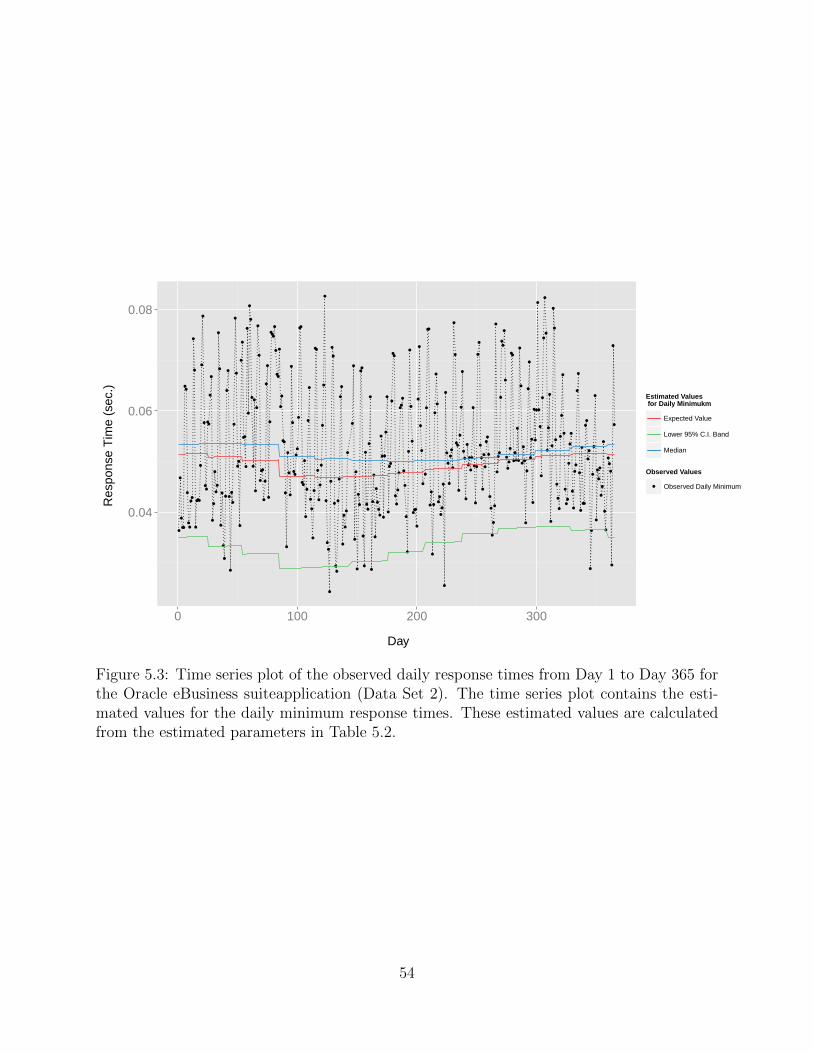
Figure 5.3 is a time series plot of Data Set 2 (black dots). The estimated expected values,median and lower limit for the 95% confidence interval are represented by the red, blue andgreen lines, respectively. Since the parameters are dependent on both t and s, the values forthese estimates are non constant. It appears that only a few of the observed daily minimumresponse time from Data Set 2 fall below the lower 95% limit.

53

0.04

0.06

0.08

0 100 200 300

Day

Res

pons

e T

ime

(sec

.)

Estimated Values for Daily Minimukm

Expected Value

Lower 95% C.I. Band

Median

Observed Values

Observed Daily Minimum

Figure 5.3: Time series plot of the observed daily response times from Day 1 to Day 365 forthe Oracle eBusiness suiteapplication (Data Set 2). The time series plot contains the esti-mated values for the daily minimum response times. These estimated values are calculatedfrom the estimated parameters in Table 5.2.

54

Alert System

One of the goals of fitting Data Set 2 to a non-stationary GEV distribution is to estimatefuture daily minimum response times and their corresponding statistics. These estimates canthen be used to create an alert system that notifies when an incomplete transaction occursin Oracle. Since Data Set 2 contains the daily minimum response times from Day 1 to Day365, the daily minimum expected value, median and the lower 95% CI limit are estimatedfor Day 366 to Day 386. These estimates are calculated from the estimated parameters inTable 5.2. The observed response times from Day 366 to Day 386 are plotted against theseestimates in order to demonstrate how an alert system can be created to detect anomaliesthat result in unsuccessful transactions.

0.0

0.1

0.2

0.3

368 372 376 380 384

Day

Res

pons

e T

ime

(sec

.)

Estimated Values for Daily Minimum

Expected Value

Lower 95% C.I. Band

Median

Observed Values

Observed Response Times

Figure 5.4: Time series plot of every observed response time from Day 366 to Day 386 for theOracle eBusiness suite application. The time series plot contains the estimated values for thedaily minimum response times. These estimated values are calculated from the estimatedparameters in Table 5.2.

Figure 5.4 contains the estimated expected values (red line), median (blue line) and lower95% CI limit (green line) for the daily minimum response times from Day 366 to Day 386.The lower 95% CI limit is interpreted as the shortest amount of time it would take for anOracle eBusiness Suite application to successfully complete a transaction. Any response timethat falls below this line suggest an unsuccessful transaction that occurred as a result of an

55

anomaly. The black dots represent every observed response time from Day 366 to Day 386.There are only three observed response times that fall below the lower limit. If this lowerlimit served as the lower threshold for an alert system,an alert would have been sent out themoment these response times occurred. This alert would have allowed for quicker anomalydetection.

We have show the importance of being alerted when a response is shorter than usual as aresult of an incomplete transaction. It is also important to be alerted when response timesare longer than usual. Therefore, the daily average response time will be modeled in orderto estimate an upper threshold for Oracle transactional response times.

56

Daily Average Response Time

Data Set 3 contains the daily average transactional response time from Day 1 to Day365. It was created in R by applying the function ddply() to Data Set 1. Data Set 3 isused to estimate and forecast the daily average response time for Oracle. The assumptionof stationarity is investigated in order to determine the most appropriate time series modelfor Data Set 3.

Checking for Stationarity

Figure 5.5 contains the time series and ACF plots of the daily average transactionalresponse time for the Oracle eBusiness Suite application from Day 1 to Day 365 (Data Set3). There appears to be a sinusoidal patter in Figure 5.5(a) and 5.5(b). This suggest thatthe time series is non-stationary with seasonal pattern. It also appears that the responsetimes from Month 10 - Month 12 in Figure 5.5(a) have an increasing trend. The KPSS testfor unit root was performed to algebraically check the stationary assumption. The results ofthe KPSS test return a p-value of .01. This indicates that there is enough evidence to rejectthe null hypothesis of unit root and assume that the data is non-stationary.

0.1

0.2

0.3

01 04 07 10 01Month

Re

sp

on

se

Tim

e (

se

c.)

(a) Time Series Plot

0 5 10 15 20 25

0.0

0.2

0.4

0.6

0.8

1.0

Lag

AC

F

(b) ACF Plot

Figure 5.5: Time series and ACF plots of the observed daily average response times fromDay 1 to Day 365 for the Oracle eBusiness Suite application (Data Set 3)

57

Model Selection

Figure 5.5 and the results of the KPSS test indicate that the data is non-stationary withboth increasing trend and seasonal pattern. Therefore, we will begin our model selection withthe seasonal ARIMA(p, q, d)[P,Q,D][s]. Since our data is collected daily, we can investigatea yearly period (s = 365), a monthly period, (s = 30) and a weekly period (s = 7). However,since the data set contains exactly 365 observations, a model with s = 365 will return thesame results as a model with s = 1 because there is only one observation per day of theyear. Therefore, we will begin our model selection by comparing ARIMA(p, q, d)[P,Q,D][s]models with s = 30 and s = 7.

The auto.arima() function in R is used to select the most appropriate time seriesmodel to describe the dependency relationship in the daily average transactional responsetimes for the Oracle eBusiness Suite application. The results suggest that the model withthe smallest AIC value is the seasonal autoregressive integrated moving average modelARIMA(2, 2, 1)[2, 1, 0]7. This implies that the time series analyses arises from a seasonalARIMA process where Yt arises from equation 5.4. With some algebra, equation 5.5 can bereduced to equation 5.5.

Φ(B7)Φ(B)D07D

1Yt = Θ(B7)Θ(B)εt (5.4)

⇒ (1−φ1B7−φ2B

14)(1−φ1B−φ2B2)DYt = (1−θ1B

7)(1−θ1B−θ2B2)εt

⇒ (1−φ1B−φ2B2− φ1B

7 +φ1φ1B8 +φ2φ1B

9− φ2B14 +φ1φ2B

15 +φ2φ2B16)(Yt−Yt−1) =

(1− θ1B − θ2B2 − θ1B

7 + θ1θ1B8 + θ1θ2B

9)εt

⇒ Yt = (1+φ1)Yt−1 + (φ2−φ1)Yt−2 − φ2Yt−3 + φ1Yt−7 − φ1(1+φ1)Yt−8 + (5.5)

φ1(−φ2 + φ1)Yt−9 + φ2φ1Yt−10 − φ2Yt−14 − φ2(1 + φ1)Yt−15 + φ2(φ1 − φ2)Yt−16 +

φ2φ2Yt−17 + εt − θ1εt−1 − θ2εt−2 − θ1εt−7 + θ1θ1εt−8 + θ1θ2εt−9

58

Dependency Relationships.

The selected orders for this model indicates that the random variable Yt has a significantcovariance with

Yt−1,Yt−2,Yt−3,Yt−7,Yt−8,Yt−9,Yt−10,Yt−14,Yt−15,Yt−16,Yt−17 and εt−1, εt−2, εt−7, εt−8, εt−9.

These significant covariance can be interpreted as follows. The selection of p = 2 impliesthat Yt has a significant covariance with the 2 previous day’s average response time (Yt−1

and Yt−1). The selection of q = 2 implies that Yt has a significant covariance with therandom errors from the two previous days (εt−1 and εt−2). The seasonal order selection ofs = 7 implies that Yt has a significant covariances with random variables and random errorsfrom previous weeks. For example, the selection of P = 2 implies that Yt has a significantcorrelation with daily response times from the previous two weeks (Yt−7 and Yt−14). Sincep = 2, Yt also has a significant correlation with Yt−8, Yt−9, Yt−15 and Yt−16. Since Q = 1,Yt has a significant correlation with the random error from the previous week (εt−7). Sinceq = 2, Yt also has a significant correlation with εt−8 and εt−9. Lastly, in order to remove thestationarity from the time series, an non-differencing operator with order d = 1 is appliedto each of the random variables in the model. This adds the random variables Yt−10 andYt−17 to the model.

Fitted Values

The estimated model parameters that are returned from fitting Data Set 3 to the seasonalARIMA(2, 2, 1)[2, 1, 0]7 model from equation 5.5 are in Table 5.3. Equation 5.6 representsthe the fitted seasonal ARIMA(2, 2, 1)[2, 1, 0]7 model.

Estimated Parameter Value

φ1 0.7417

φ2 0.1986ˆφ1 0.9551ˆφ2 0.0359

θ1 0.1063

θ1 -0.7900ˆθ1 -0.8669

Table 5.3: The estimated model parameter coefficients for the seasonalARIMA(2, 2, 1)[2, 1, 0]7 model.

59

⇒ yt = (1 + φ1)yt−1 + (φ2 − φ1yt−2 − φ2yt−3 +ˆφ1yt−7 −

ˆφ1(1 + φ1yt−8 + (5.6)

ˆφ1(−φ2 + φ1)yt−9 + φ2

ˆφ1yt−10 −

ˆφ2yt−14 −

ˆφ2(1 + φ1)yt−15 +

ˆφ2(φ1 − φ2)yt−16 +

φ2ˆφ2yt−17 + εt − θ1εt−1 − θ2εt−2 −

ˆθ1εt−7 +

ˆθ1θ1εt−8 +

ˆθ1θ2εt−9

Once the estimated values from Table 5.3 are plugged into equation 5.6, the set of fittedvalue, denoted by y1:365, are calculated directly from equation 5.6. The set y1:365 representthe estimated daily average transactional response times from Day 1 to Day 365. Figure 5.6is Data Set 3 (black dotted line) plotted against y1:365 (red line). The fitted values appearto model the data appropriately and residual diagnostics were analyzed and confirm anappropriate fit.

0.1

0.2

0.3

0 100 200 300

Day

Res

pons

e T

ime

(sec

.)

Estimated Values for Daily Average

Expected Value (fitted values)

Observed Values

Observed Daily Average

Figure 5.6: A time series plot of the observed daily average response times from Day 1 to Day365 for the Oracle eBusiness Suite application (Data Set 3). The time series plot containsthe estimated daily average values. These values are calculated from the fitted seasonalARIMA(2, 2, 1)[2, 1, 0]7 model (eqn. 5.6).

60

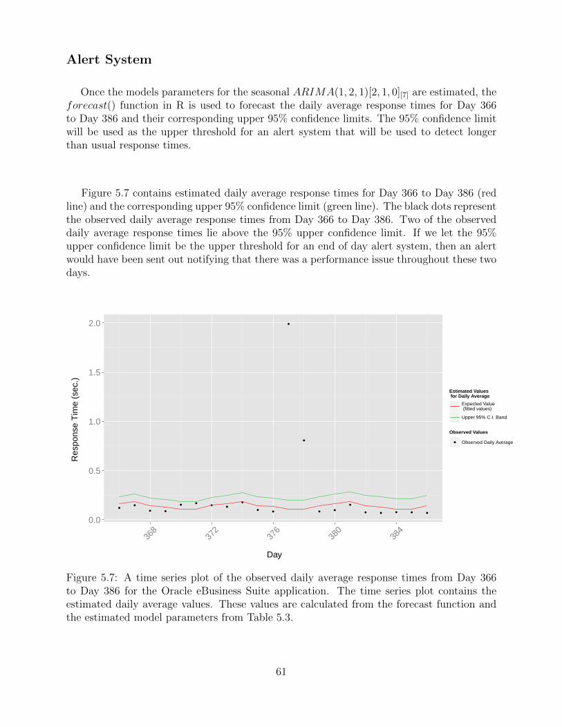
Alert System

Once the models parameters for the seasonal ARIMA(1, 2, 1)[2, 1, 0][7] are estimated, theforecast() function in R is used to forecast the daily average response times for Day 366to Day 386 and their corresponding upper 95% confidence limits. The 95% confidence limitwill be used as the upper threshold for an alert system that will be used to detect longerthan usual response times.

Figure 5.7 contains estimated daily average response times for Day 366 to Day 386 (redline) and the corresponding upper 95% confidence limit (green line). The black dots representthe observed daily average response times from Day 366 to Day 386. Two of the observeddaily average response times lie above the 95% upper confidence limit. If we let the 95%upper confidence limit be the upper threshold for an end of day alert system, then an alertwould have been sent out notifying that there was a performance issue throughout these twodays.

0.0

0.5

1.0

1.5

2.0

368

372

376

380

384

Day

Res

pons

e T

ime

(sec

.)

Estimated Values for Daily Average

Expected Value (fitted values)

Upper 95% C.I. Band

Observed Values

Observed Daily Average

Figure 5.7: A time series plot of the observed daily average response times from Day 366to Day 386 for the Oracle eBusiness Suite application. The time series plot contains theestimated daily average values. These values are calculated from the forecast function andthe estimated model parameters from Table 5.3.

61

Using the upper 95% confidence limit as the upper threshold for an end of the day alertsystem is beneficial for solving performance issues. However, it is important to send out analert the moment a pattern of long response times that are a result of a performance issuestarts to occur. Therefore, the estimated hourly average response time will be estimated inorder to have an hourly alert system.

Hourly Average Response Time

The methodology used to estimate the hourly average response time is identically tothe methodology used to model the daily average response time. The data set that is usedto estimate and forecast the daily average response time for the Oracle eBusiness Suiteapplication is created in R by applying the function ddply() to Data Set 1. This returns adata set that contains the hourly average transactional response time from Day 1 to Day365 (Data Set 4).

Checking for Stationarity

Figure 5.8 contains the time series and ACF plots of the hourly average transactionalresponse time for the Oracle eBusiness Suite application from Day 1 to Day 365 (Data Set4). Both Figures 5.8(a) and 5.8(b) appear to have a slight seasonal trend. The results of theKPSS test return a p-value of 0.01. This indicates that there is there is enough evidence toreject the null hypothesis of unit root and we may assume that the data is non-stationary.Since both the diagnostic plots and KPSS test suggest non-stationarity, we will begin ourmodel selection with the ARIMA(p, q, d)[P,Q,D][s] model.

Model Selection

The results of applying the auto.arima() function to Data Set 4 selects an ARIMA(1, 2, 1)(0, 1, 0)[24] as the most appropriate time series model to describe the dependency relationshipin the hourly average transactional response times for the Oracle eBusiness Suite application.This implies that Yt arises from the autoregressive model

[1− φ1B]D1Yt = [1− θ1B24][1− θ1B − θ2B

2]εt. (5.7)

The selected model parameters imply that the differenced hourly average response time forthe Oracle eBusiness Suite application depends only on the previous hour’s average responsetime. Whereas, an hour’s random error depends on the 2 previous hours’ random errors andthe random error from 24 hours prior.

62

0

1

2

3

4

01 04 07 10 01Month

Re

sp

on

se

Tim

e (

se

c.)

(a) Time Series Plot

0.0 0.5 1.0 1.5

0.0

0.2

0.4

0.6

0.8

1.0

Lag

AC

F

ACF Plot

(b) ACF Plot

Figure 5.8: Time series and ACF plot of the observed hourly average response times fromDay 1 to Day 365 for the Oracle eBusiness Suite application (Data Set 4).

Fitted Values

The fitted ARIMA(1, 2, 1)(0, 1, 0)[24] model that is used to calculate the estimated hourlyaverage response times is

[1− φ1B]D1yt = [1− ˆθ1B

24][1− θ1B − θ2B2]εt, (5.8)

where φ1 = 0.362, θ1 = −1.1745, θ2 = 0.1756 andˆθ1 = 0.0119 are the values of the estimated

parameters. The value yt represents the estimated average response time for hour t and εtrepresents the difference between the observed and estimated average response for hour t,where εt = yt − yt.

Figure 5.9 contains a plot of the estimated hourly average response times calculated fromthe fitted model (red line) against the observed hourly average response times (black dottedline) for the Oracle eBusiness Suite application from Day 1 to Day 365. The fitted valuesappear to fit the observed data well and appropriate residual diagnostics were performedand confirm an appropriate fit.

63

0

1

2

3

4

50 100 150 200 250 300 350

Days

Res

pons

e T

ime

(sec

.)

Estimated Values for Hourly Average

Expected Value (fitted values)

Observed Values

Observed Hourly Average

Observed Hourly Average

Figure 5.9: A time series plot of the observed hourly average response times from Day 1to Day 365 for the Oracle eBusiness Suite application (Data Set 4). The time series plotcontains the estimated hourly average values. These values are calculated from the fittedARIMA(1, 2, 1)(0, 1, 0)[24] model (eqn. 5.8).

Alert System

Figure 5.10 contains a plot of the estimated hourly response times (red line) for Day 366to Day 386 and the corresponding 95% upper limit (green line). The black dots representthe observed hourly average response times from Day 366 to Day 386. There appears to bea few hourly average response times that are greater than the 95% upper limit.

Most of the long hourly average response times were observed occurred between Days378 and 379. The Oracle eBusiness Suite application was investigated after this analysis wasperformed and it was discovered that on Day 377, the application had a power outage thatresulted in unrecorded response times and large response times from Days 378 and 379. Ifthis alert system was implemented at the time of this power outage and the upper limit wasused as the upper threshold from an alert system, an alarm would have been sent out themoment the first unusually long hourly average response time occurred.

64

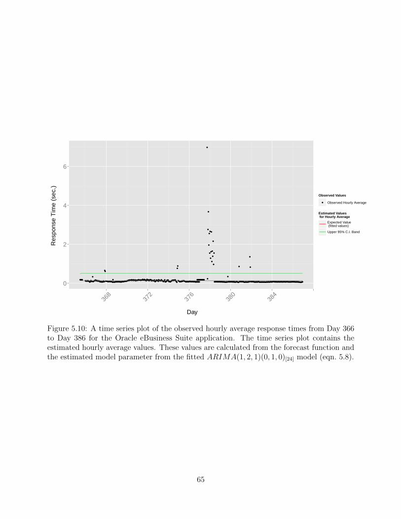
0

2

4

6

368

372

376

380

384

Day

Res

pons

e T

ime

(sec

.)

Observed Values

Observed Hourly Average

Estimated Values for Hourly Average

Expected Value (fitted values)

Upper 95% C.I. Band

Figure 5.10: A time series plot of the observed hourly average response times from Day 366to Day 386 for the Oracle eBusiness Suite application. The time series plot contains theestimated hourly average values. These values are calculated from the forecast function andthe estimated model parameter from the fitted ARIMA(1, 2, 1)(0, 1, 0)[24] model (eqn. 5.8).

65

66

Chapter 6

Implementation to Weblogic c12Server Application

Introduction

The data used to analyze Weblogic c12 Server application’s transactional response timeare from the transactional tests that are performed every five minutes on the Weblogic c12Server application. Like the Oracle eBusiness suite application, the data is stored in Nagios.Data Set 5 contains the recorded transactional response times from the tests that wereperformed from Day 1 to Day 365. Each recording from this data set contains two elements,an unformatted time stamp (GMT time zone) and its corresponding transactional responsetime (seconds). The recorded data from Day 366 to 386 is used to test the accuracy of theestimations calculated from Data Set 5. Since the methodology used to perform this analysisis identical to the methodology described in Chapter 5, we will start by discussing the resultsof estimating the non-staionary GEV Distribution for the daily minimum response times.

Daily Minimum Response Time

Results

Figure 6.1 is a time series plot of the daily minimum response times from Day 1 to Day365 for the Weblogic c12 Server application (black dotted line). It contains the estimatedWeblogic c12 server application’s expected daily minimum response times (red line), thecorresponding 95% lower confidence limit (green line)and the estimated median (blue line).Appropriate residual diagnostics were performed and suggest that there is an appropriatefit. Figure 6.2 contains every observed response time from Day 366 to Day 386 and theforecasted daily minimum response time for the Weblogic c12 Server application. On Day368, there appears to be six observed response times that fell below the lower limit. If thelower limit was used as the lower threshold for an alert system, an alarm would have beensent out the moment the first unusually short response time fell below the threshold. Thiswould have allowed for a quicker and more accurate anomaly detection.

67

0.05

0.10

0.15

0.20

0 100 200 300

Day

Res

pons

e T

ime

(sec

.)

Estimated Values for Daily Minimukm

Expected Value

Lower 95% C.I. Band

Median

Observed Values

Observed Daily Minimum

Figure 6.1: A time series plot of the observed daily minimum response times from Day 1 toDay 365 for the Weblogic c12 Server application. The time series plot contains the estimateddaily minimum response times. These estimated values are calculated from the estimatedparameters from the fitted non-stationary GEV distribution.

68

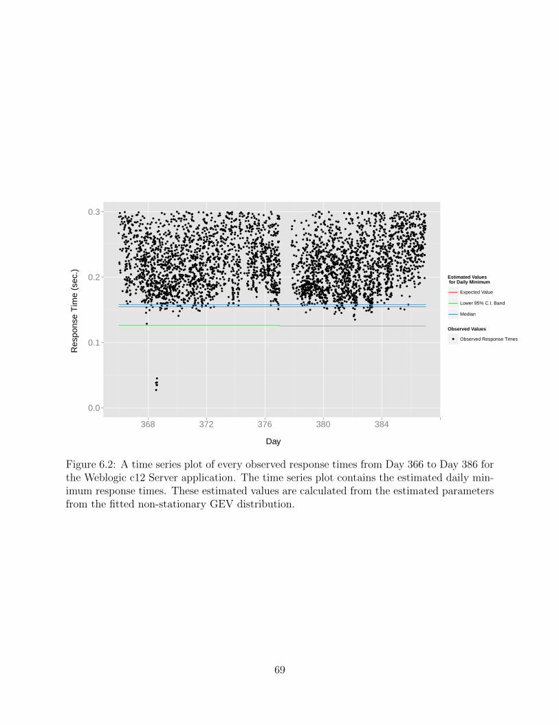
0.0

0.1

0.2

0.3

368 372 376 380 384

Day

Res

pons

e T

ime

(sec

.)

Estimated Values for Daily Minimum

Expected Value

Lower 95% C.I. Band

Median

Observed Values

Observed Response Times

Figure 6.2: A time series plot of every observed response times from Day 366 to Day 386 forthe Weblogic c12 Server application. The time series plot contains the estimated daily min-imum response times. These estimated values are calculated from the estimated parametersfrom the fitted non-stationary GEV distribution.

69

Hourly Average Response Time

Results

Since having a continuous alert system is more beneficial than having an end of dayalert system, we will only discuss the results of modeling Weblogic c12 server application’shourly average response time. The model that is selected as the most appropriate modelto estimate the hourly average response times and forecast future response times is a non-seasonal ARIMA(2, 2, 0) model.

Figure 6.3 is a time series plot of Weblogic c12 server application’s observed hourlyaverage response times for Day 1 to Day 365 (block dotted line). The red line represents theestimated expected values for the hourly average response times that were calculated fromthe fitted non-seasonal ARIMA(2, 2, 0) model.

Figure 6.4 contains the foretasted hourly average response times for Day 366 to Day 386and the corresponding 95% upper confidence limit. The black dots represent the observedhourly average response times from Day 366 to Day 386. There appears to be some hourlyaverage response times that are greater than the upper limit; especially between Days 378and 379. Days 378 and 379 are the dates that the power outage on Day 377 affected theOracle eBussiness suite application’s response times. Further investigation was done onthe Weblogic c12 server application, and it was found that the power outage affected thisapplication as well. If the upper limit served as the upper threshold for an alert system, anotification of these long response times would have been sent the moment they had startedto occur; this would have allowed for quicker anomaly detection.

70

0

4

8

12

50 100 150 200 250 300 350

Days

Res

pons

e T

ime

(sec

.)

Estimated Values for Hourly Average

Expected Value (fitted values)

Observed Values

Observed Hourly Average

Observed Hourly Average

Figure 6.3: A time series plot of the observed hourly average response times from Day1 to Day 365 for the Weblogic c12 Server application. The time series plot contains theestimated hourly average response times. These estimated values are calculated from thefitted non-seasonal ARIMA(2, 2, 0) model.

71

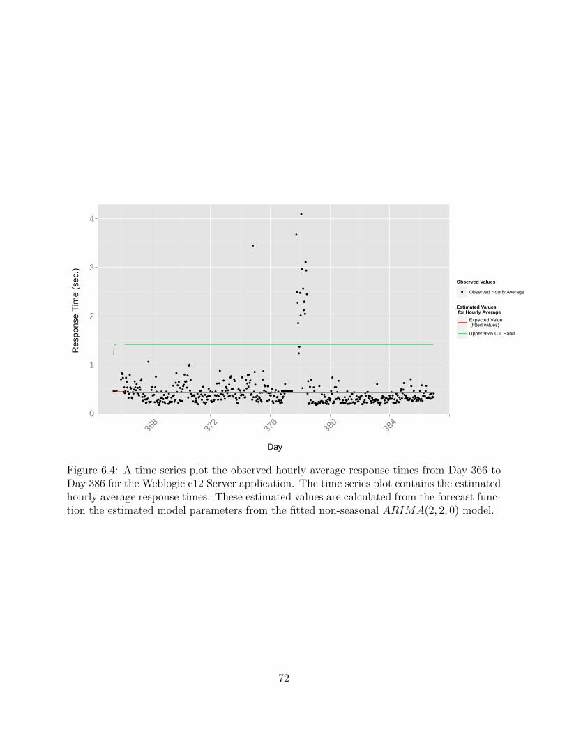
0

1

2

3

4

368

372

376

380

384

Day

Res

pons

e T

ime

(sec

.)

Observed Values

Observed Hourly Average

Estimated Values for Hourly Average

Expected Value (fitted values)

Upper 95% C.I. Band

Figure 6.4: A time series plot the observed hourly average response times from Day 366 toDay 386 for the Weblogic c12 Server application. The time series plot contains the estimatedhourly average response times. These estimated values are calculated from the forecast func-tion the estimated model parameters from the fitted non-seasonal ARIMA(2, 2, 0) model.

72

Chapter 7

Conclusion

The theoretical minimum response time of an application serves as a basis for the ap-plication’s expected response time. We have shown through the Oracle eBusiness Suite andWeblogic c12 Server applications that estimating the daily minimum response time resultsin an estimated lower limit. This estimated lower limit represents the minimum amount oftime that the application should take to complete any transaction on that day. When anapplication’s response time is greater than a certain threshold, there is likely an anomalyin the application that is causing unusual performance issues. We have also shown thatestimating the distribution of the theoretical average response time can be used to calculatethe value of this threshold.

Since Sandia National Laboratory’s Application Services and Analytics departments mid-dleware services provide support to the entire laboratory, it is important that we researchand implement analytic capabilities that can improve our understanding of an applicationstransactional response time. Therefore, it is beneficial to implement the findings of thisresearch to all types of transactional applications that are being used by the ApplicationServices and Analytics departments. Implementing these methods will result in quicker andmore accurate anomaly detection that will lead to better problem management.

73

74

References

[1] Canova, F., Hansen, B (1995). ‘Are seasonal patterns constant over time? a test forseasonal stability’. Journal of Business and Economic Statistics, (13):237-252.

[2] Casella, G., and Berger, R. (2002). Statistical inference (2nd ed.). Australia: ThomsonLearning.

[3] Coles, S. (2001). An Introduction to Statistical Modeling of Extreme Values. Springer-Verlag, London, U.K.

[4] Haan, L. De, and Ferreira, A. (2006). Extreme Value Theory: An Introduction. NewYork: Springer.

[5] Heffernan, J and Stephenson, A (2012). ismev: An Introduction to Statisti-cal Modeling of Extreme Values. R package version 1.39. URL http://CRAN.R-project.org/package=ismev.

[6] Hyndman, R. et al (2015). forecast: Forecasting functions for time series and linearmodels. R package version 5.6. URL http://CRAN.R-project.org/package=forecast.

[7] Hyndman, R. and Khandakar, Y. (2008) ”Automatic time series forecasting: The forecastpackage for R”, Journal of Statistical Software, 26(3).

[8] Kwiatkowski D, Phillips PC, Schmidt P, Shin Y (1992). ‘Testing the Null Hypothesis ofStationarity Against the Alternative of a Unit Root’. Journal of Econometrics, 54, 159 -178.

[9] Peiris, M. and Perera, B. (1988), ’On prediction with fractionally differenced ARIMAmodels”, Journal of Time Series Analysis, 9(3), 215-220.

[10] Prado, Raquel, and Mike West (2010). Time Series: Modeling, Computation, and In-ference. Boca Raton: CRC.

[11] R Core Team (2013). R: A language and environment for statistical computing. R Foun-dation for Statistical Computing, Vienna, Austria. URL http://www.R-project.org/.

[12] West, Mike. Electroencephalogram Recordings. Department of Statistical Science DukeUniversity.

[13] Wickham, Hadley (2011). The Split-Apply-Combine Strategy for Data Analysis. Journalof Statistical Software, 40(1), 1-29.

75

76

Appendix A

Hyndman and Khanadakar ARIMAModel Selection Algorithm

The following is a summary of the Hyndman and Khanadakar ARIMA model selectionalgorithm that can be found in the Statistical Journal, ”Automatic time series forecasting:The forecast package for R”. The algorithm is used in the auto.arima() function in R [7].

A.0.1 Non-Seasonal: s = 1

Saturated Model: ARIMA(p, q, d)

Step 1:

Select d using the KPSS unit-root test explained in section 2.2.1. This involves in-creasing the value of d until the KPSS unit-root test returns an insignificant result. The firstvalue of d that returns an insignificant result will be selected for the model.

Step 2:

Fit the following four models using the function arima() in R programming:

1. ARIMA(2, d, 2)

2. ARIMA(0, d, 0)

3. ARIMA(1, d, 0)

4. ARIMA(0, d, 1)

If d ≤ 1 then these models are fit with c 6= 0. Select the model that has the smallest AICvalue, where AIC = 2(p+ q +K)− 2ln(L),

77

and where k = 1 if c 6= 0 and L is the maximized likelihood of the model fitted to thenon-seasonal differenced data Ddyt. The selected model will be called the “current” model.

Step 4:

Fit the following variations of the “current” model from Step 3 where:

1. One of the model orders p and q varies by ±1 from the current model.

2. Both model order p and q vary by ±1 from the current model.

3. Either include or exclude the parameter c, depending on if it’s included in the “current”model.

If the AIC value one of the variations of the “current” model has a lower AIC value then the“current” model, then it becomes the new ”current model”. After all variations have beenfitted, the “current” model is selected as the most appropriate model.

In order to avoid problems with convergence or near unit roots, Hyndman andKhandakargive a list of constraints that can be found in their Journal of Statistical software [7].

A.0.2 Seasonal: s 6= 1

Saturated Model: ARIMA(p, q, d)(P,DQ,D)[s]

Step 1:

Select D, where D = 0 or 1, using the Canova-Hansen Test. The Canova-Hansen Testchecks whether the change seasonal pattern of a realization changes sufficiently over timeleads to a unit root. Further discussion of this test can be found in Canoca and Hansen 1995[1].

Step 2:

Select d by applying the KPSS unit-root test, section 2.2.1, to the seasonal differenceddata DD

s yt. This involves increasing the value of d until the KPSS unit-root test returns aninsignificant result. The first value of d that returns an insignificant result will be selectedfor the model.

78

Step 3:

Fit the following four models using the function arima() in R programming:

1. ARIMA(2, d, 2)(1, D, 1)[s]

2. ARIMA(0, d, 0)(0, D, 0)[s]

3. ARIMA(1, d, 0)(1, D, 0)[s]

4. ARIMA(0, d, 1)(0, D, 1)[s]

If D + d ≤ 1, then these models are fit with c 6= 0. Select the model that have the smallestAIC value, where AIC = 2(p+ q + P +Q+ k)− 2ln(L), and where k = 1 if c 6= 0 and L isthe maximized likelihood of the model fitted to the differenced data, Dd

sDdyt. The selected

model will be called the “current” model.

Step 4:

Fit the following variations of the “current” model from Step 3 where:

1. One of the model orders p, q, P and Q varies by ±1 from the current model.

2. Both model order p and q vary by ±1 from the current model.

3. Both model order P and Q vary by ±1 from the current model.

4. Either include or exclude the parameter c, depending on if it’s included in the “current”model.

If the AIC value one of the variations of the “current” model has a lower AIC value then the“current” model, then it becomes the new ”current model”. After all variations have beenfitted, the “current” model is selected as the most appropriate model.

In order to avoid problems with convergence or near unit roots, Hyndman andKhandakargive a list of constraints that can be found in their Statistical Journal, ”Automatic time seriesforecasting: The forecast package for R” [7].

79

DISTRIBUTION:

1 MS 0805 W.R. Cook, 09530 (electronic copy)

1 MS 0820 J.P. Abbott, 09339 (electronic copy)

1 MS 0838 G.K. Rogers, 09330 (electronic copy)

1 MS 0933 J.O. Gallegos, 09500 (electronic copy)

5 MS 1465 M.R. Paiz, 09533

1 MS 1465 M.R. Paiz, 09533 (electronic copy)

1 MS 1465 G.N. Conrad, 09533 (electronic copy)

1 MS 0899 Technical Library, 9536 (electronic copy)

80

v1.40

81

82