Model uncertainty and its impact on the pricing

of derivative instruments.

Rama CONTCentre de Mathematiques Appliquees

Ecole Polytechnique F-91128 Palaiseau, France.

To appear in: Mathematical Finance. ∗

Keywords: model uncertainty, Knightian uncertainty, option pricing, incom-plete markets, volatility, ambiguity, coherent risk measures, convex risk mea-sures.

Abstract

Uncertainty on the choice of an option pricing model can lead to“model risk” in the valuation of portfolios of options. After discussingsome properties which a quantitative measure of model uncertainty shouldverify in order to be useful and relevant in the context of risk managementof derivative instruments, we introduce a quantitative framework for mea-suring model uncertainty in the context of derivative pricing. Two meth-ods are proposed: the first method is based on a coherent risk measurecompatible with market prices of derivatives, while the second method isbased on a convex risk measure. Our measures of model risk lead to a pre-mium for model uncertainty which is comparable to other risk measuresand compatible with observations of market prices of a set of benchmarkderivatives. Finally, we discuss some implications for the management of“model risk”.

∗This project was supported by a research grant from the Europlace Institute of Finance.Part of this work was done in the framework of a research project on model uncertaintyat HSBC-CCF, Division of Market and Model Risk. Previous versions of this work werepresented at the Hermes Center (Nicosia), 3rd METU Economics Research Conference (2003),the European conference on Arbitrage theory and applications (Paris, 2003) and the Workshopon Advanced Mathematical Methods in Finance (Munich, 2004). We thank Sana BenHamida,Joel Bessis, Jean-Francois Boulier, Remi Bourrette, Nicole El Karoui, Larry Epstein, DanielGabay, Jocelyne Nadal, Walter Schachermayer, Franck Viollet and an anonymous referee forhelpful comments and Emmanuelle Hammerer for research assistance.

1

Contents

1 Introduction 3

2 Risk, uncertainty and ambiguity 52.1 Bayesian model averaging . . . . . . . . . . . . . . . . . . . . . . 62.2 Worst case approaches . . . . . . . . . . . . . . . . . . . . . . . . 72.3 Risk measures . . . . . . . . . . . . . . . . . . . . . . . . . . . . . 8

3 Model uncertainty in the context of derivative valuation 103.1 Statistical uncertainty vs uncertainty on pricing rules . . . . . . . 103.2 Benchmark instruments vs illiquid products . . . . . . . . . . . . 113.3 Requirements for a measure of model uncertainty . . . . . . . . . 11

4 A quantitative framework for measuring model uncertainty 124.1 An axiomatic setting for model uncertainty . . . . . . . . . . . . 134.2 A “coherent” measure of model uncertainty . . . . . . . . . . . . 154.3 Examples . . . . . . . . . . . . . . . . . . . . . . . . . . . . . . . 164.4 Robustness of hedging strategies to model uncertainty . . . . . . 22

5 A convex measure of model uncertainty 22

6 Discussion 276.1 Summary . . . . . . . . . . . . . . . . . . . . . . . . . . . . . . . 276.2 Specifying the class of models . . . . . . . . . . . . . . . . . . . . 286.3 Updating with new information . . . . . . . . . . . . . . . . . . . 286.4 Conclusion . . . . . . . . . . . . . . . . . . . . . . . . . . . . . . 29

A Proof of Proposition 1 33

B Proof of Proposition 2 34

2

1 Introduction

In March 1997, Bank of Tokyo/Mitsubishi announced that its New York-basedderivatives unit had suffered a $ 83 million loss because their internal pricingmodel overvalued a portfolio of swaps and options on U.S. interest rates. A fewweeks later, NatWest Capital Markets announced a £50 million loss because of amispriced portfolio of German and U.K. interest rate options and swaptions runby a single derivatives trader in London. According to observers having followedthese events, many “of the situations [..] that led to (recent) derivatives losseswere attributable to model risk” [Elliott (1997)].

With the dissemination of quantitative methods in risk management and ad-vent of complex derivative products, mathematical models have come to play anincreasingly important role in financial decision making, especially in the con-text of pricing and hedging of derivative instruments. While the use of modelshas undeniably led to a better understanding of market risks, it has in turn givenrise to a new type of risk, known as “model risk” or “model uncertainty”, linkedto the uncertainty on the choice of the model itself. According to a recent report[Williams (1999)], $ 5 billion in derivatives losses in 1999 were attributable to“model risk”.

Uncertainty on the choice of the pricing model can lead to the mispricingof derivative products. While model uncertainty is acknowledged by most op-erators who make use of quantitative models, most of the discussion on thissubject has stayed at a qualitative level and a quantitative framework for mea-suring model uncertainty is still lacking. As noted by [Williams (1999)], “thereare no packaged, off-the-shelf systems for model risk management”. Some ques-tions for which one would like quantitative answers are:

• How sensitive is the value of a given derivative to the choice of the pricingmodel?

• Are some instruments more model-sensitive than others?

• How large is the model uncertainty of a portfolio compared with its marketrisk?

• Can one provision for “model risk” in the same way as one provisions formarket risk and credit risk?

One could wonder whether model uncertainty deserves a separate treatmentfrom other sources of uncertainty in financial markets. Indeed, the classicalapproach to decision under uncertainty [Savage] does not distinguish betweendifferent sources of risk: “model uncertainty” should be indistinguishable frommarket risk, credit risk,...which would imply that ”model uncertainty” simplyamounts to weighting various models with probabilities and representing allsources of uncertainty using a probability distribution on the enlarged spacecomprising “models” + scenarios. Indeed, such “model averaging” approacheshave been proposed in the Bayesian literature [Hoeting et al.] (see Section 2).However, this approach is in strong contrast with the current practices in risk

3

management: as noted by [Routledge & Zin (2001)], market participants typi-cally use different criteria to measure “market risk” and “model risk”, the for-mer being valued by using a probabilistic model while the latter is approachedthrough a worst case approach, for instance by stress testing of portfolios.

This had led to the distinction between risk -uncertainty on outcomes forwhich the probabilities are known- and ambiguity or model uncertainty-whenseveral specifications are possible for such probabilities [Knight]. [Ellsberg]has shown that aversion to ambiguity clearly plays a role in decision mak-ing. A growing body of literature has explored decision under ambiguity, itsaxiomatic foundations [Gilboa & Schmeidler, Epstein] and implications for thebehavior of security prices [Epstein & Wang, Routledge & Zin (2001)]. Some ofthese ideas have resurfaced in the recent literature on coherent risk measures[Artzner et al(1999)] and their extensions [Follmer & Schied (2002)].

Although general in nature, these approaches do not take into account somespecific features of the use of probabilistic models in the pricing of derivatives.The notion of coherent risk measure does not distinguish hedgeable and non-hedgeable risks, nor does it differentiate between market risk and model un-certainty. And, although coherent measures of risk are expressed in monetaryunits, when applied to traded options they may lead to numbers which are notnecessarily comparable to the mark-to-market value of these options. Also, inthe context of derivative pricing, models are often specified not in terms of ob-jective probabilities but “risk-neutral” probabilities so, in incomplete markets,ambiguity can prevail on pricing criteria even when there is no ambiguity onthe underlying price process itself. These remarks show that model uncertaintyin option pricing cannot be reduced to the classical setting of decision underambiguity and merits a specific treatment.

We attempt to address these issues by defining a framework for quantify-ing model uncertainty in option pricing models. We first discuss, at an intuitivelevel, some properties which a quantitative measure of model uncertainty shouldpossess in order to qualify as a measure of model uncertainty in the context ofrisk measurement and management. We then propose two methods for mea-suring model uncertainty which verify these properties and are compatible withobservations of market prices of a set of benchmark derivatives: our first methodis based on a set of pricing models calibrated to the benchmark options, whilethe second method relaxes the calibration requirement. Both methods lead toa decomposition of risk measures into a market value and a premium for modeluncertainty.

The paper is structured as follows. We start by discussing some existingapproaches to decision-making in presence of multiple probability measures inSection 2. Some specific features of the use of models in the valuation of deriva-tive instruments are not taken into account in these general frameworks; theseissues are discussed in Section 3, where we give an intuitive definition of modeluncertainty in the context of derivative markets and enumerate some propertiesa measure of model uncertainty must have in order to be meaningful for riskmanagement of derivative instruments. In Section 4 we formulate these require-ments in mathematical terms and present a methodology for measuring model

4

uncertainty which verifies these requirements. This method requires to specifya set of pricing models and calibrate them to a set of market option prices;this requirement is relaxed in Section 5, where a more general approach basedon convex risk measures is proposed. Section 6 concludes by summarizing ourmain contributions, discussing some open questions and pointing out possibleimplications of our work for the measurement and management of “model risk”.We have attempted to motivate the mathematical notions introduced throughexamples which illustrate their relevance.

2 Risk, uncertainty and ambiguity

The starting point in option pricing theory is usually the specification of astochastic model: a set of future scenarios (Ω,F) and a probability measure P

on these outcomes. However there are many circumstances in financial decisionmaking where the decision maker or risk manager is not able to attribute a pre-cise probability to future outcomes. This situation has been called “uncertainty”by [Knight], by contrast with “risk”, when we are able to specify a unique prob-ability measure on future outcomes.1 More precisely, we speak of ambiguitywhen we are facing several possible specifications P1, P2, .. for probabilities onfuture outcomes [Epstein].

In his 1961 thesis, [Ellsberg] established a distinction between aversion torisk–related to lack of knowledge of future outcomes– and aversion to ambi-guity2, related to the lack of knowledge of their probabilities, and showedthat aversion to ambiguity can strongly affect decision makers behavior andresolve some paradoxes of classical decision theory. More recently, ambigu-ity aversion has shown to have important consequences in macroeconomics[Hansen et al., 1999, Hansen et al.] and for price behavior in capital markets[Chen & Epstein, Epstein & Wang, Routledge & Zin (2001)].

Two different paradigms have been proposed for evaluating uncertain out-comes in presence of ambiguity. The first one, which consists of averaging overpossible models, has been used in the statistical literature [Raftery, Hoeting et al.].The other one is based on worst-case or “maxmin” approach and has been ax-iomatized by [Gilboa & Schmeidler] and studied in the context of asset pric-ing by [Epstein & Wang, Routledge & Zin (2001)] and others. Related to thisworst-case approach is the recent literature on coherent measures of risk [Artzner et al(1999)].We review in this section these approaches and their possible implications andshortcomings for quantifying model uncertainty for portfolios of derivatives.

1This distinction appeared in [Knight], hence the term “Knightian uncertainty” sometimesused to designate the situation where probabilities are unknown. We remark here that theterm “model risk” sometimes used in the financial literature is somewhat confusing in thisrespect and the term “model uncertainty” should be preferred.

2We use here the terminology of [Epstein].

5

2.1 Bayesian model averaging

A lot of attention has been devoted to model uncertainty in the context of sta-tistical estimation, using a Bayesian approach. [Hoeting et al.] note that “dataanalysts typically select a model from some class of models and then proceedas if the selected model had generated the data. This approach ignores the un-certainty in model selection, leading to over-confident inferences and decisionsthat are more risky than one thinks they are”. Bayesian model averaging is oneway to incorporate model uncertainty into estimation procedures.

Let M = M1, ...,MJ be a family a of candidate models whose parameters(not necessarily in the same sets) are denoted by θ1 ∈ E1, ..., θJ ∈ EJ . Considera Bayesian observer with two levels of prior beliefs:

• Priors on model parameters: p(θj |Mj) is a prior density (on Ej) thatsummarizes our views about the unknown parameters of model j, giventhat Mj holds.

• Prior “model weights”: P(Mj), j = 1..J , the prior probability that Mj isthe “true” model.

Given a set of observations y, the posterior probability for model Mj is

P(Mj |y) =p(y|Mj)P(Mj)∑J

k=1 p(y|Mk)P(Mk)(2.1)

where p(y|Mj) is the integrated likelihood of the data under model Mj :

p(y|Mj) =∫

Ek

P(y|θj ,Mj)p(θj |Mj) dθj (2.2)

Suppose we want to compute a model dependent quantity, given by the expec-tation of a random variable X: we only have the observations y but we areuncertain about the model to use. The Bayesian model averaging approachsuggests to compute this quantity in each model and average over the models,weighting each model by its posterior probability given the observations:

E[X|y] =m∑

j=1

E[X|y,Mj ] P(Mj |y) (2.3)

If Mj are alternative option pricing models, this would amount to computingoption prices in each model and taking a weighted average across models. Sim-ilarly one can use the following quantity to measure dispersion across models:

D[X|y] =m∑

j=1

E[X|y,Mj ] − E[X|y]2 P(Mj |y) (2.4)

Averaging across models, whether or not it is done in a Bayesian way, providesa higher stability of the estimates obtained. However, several obstacles appearwhen trying to apply this approach in the framework of option pricing.

6

First, this method not only requires specifying –as in any Bayesian method–a prior p(θj |Mj) on parameters of each model, but also a prior probability P(Mj)on possible models, which is more delicate. How does one weigh a stochasticvolatility model with respect to a jump-diffusion model? How should priorweights vary with the number of factors in interest rate models? While suchquestions might be ultimately reasonable to ask, not much experience is availablein assigning such prior weights.3 In other words, this approach requires too muchprobabilistic sophistication on the part of the end user.

The second obstacle is computational: the posterior distributions involvedin the formulas above are not explicit and sampling from them requires theuse of Markov Chain Monte Carlo algorithms, which are computationally inten-sive. Such an approach has been attempted in the case of Black-Scholes model[Jacquier & Jarrow (2000)] but seems less feasible as soon as we move to morecomplex models. It should also be noted that, because of these computationaldifficulties, the Bayesian model averaging literature deals with relatively simplemodel structures (linear and regression-type models).

Overall, the main justification for averaging over models is that it improvespredictive ability [Hoeting et al.] of some target quantity (say, an option price).However, the main concern of risk management is not to predict prices but toquantify the risk associated with them so model averaging seems less relevantin this context.

2.2 Worst case approaches

The model averaging procedure described above, whether or not it is done in aBayesian way, is in fact consistent with the classical approach to decision underuncertainty [Savage], which does not distinguish between different sources ofrisk: in this approach, “model uncertainty” should be indistinguishable frommarket risk, credit risk,...“Model uncertainty” then simply amounts to weightingvarious models with probabilities and representing all sources of uncertaintyusing a probability distribution on the enlarged space comprising “models” +scenarios. However, this approach is in strong contrast with the current practicesin risk management: market participants do not specify probabilistic beliefsover models and, as noted by [Routledge & Zin (2001)], typically use differentcriteria to measure “market risk” and “model risk”, the former being valued byrisk neutral pricing (averaging across scenarios) while the latter is approachedthrough a worst case approach, for instance by stress testing of portfolios.

Aside from being observed in the practice of risk managers, the worst-caseapproach also has a firm axiomatic foundation: [Gilboa & Schmeidler] proposea system of axioms under which an agent facing ambiguity chooses among a setA of feasible alternatives by maximizing a “robust” version of expected utility(also called “maxmin” expected utility), obtained by taking the worst case overall models:

maxX∈A

minP∈P

EP[U(X)] (2.5)

3In the statistical literature, uniform priors on models are often used.

7

Here the risk aversion of the decision maker is captured by the utility functionU , while the aversion to ambiguity (model uncertainty) is captured by takingthe infimum over all models in P. The worst case approach clearly distinguishesmodel uncertainty from risk: the latter is treated by averaging over scenarioswith a given model while the former is treated by taking the supremum overmodels. With respect to model averaging procedures described in Section 2.1,worst case approaches are more conservative, more robust and require less so-phisticated inputs on the part of the user. Thus, they are more amenable to thedesign of a robust, systematic approach for measuring model uncertainty.

2.3 Risk measures

Related to the worst case approach described above is the notion of coherent riskmeasure. A risk measurement methodology is a way of associating a number(“risk measure”) ρ(X) with a random variable X, representing the payoff ofan option, a structured product or a portfolio. More precisely, if we define apayoff as a (bounded measurable) function X : Ω → R defined on the set Ωof market scenarios and denote the set of payoffs as E, then a risk measure isa map ρ : E → R. [Artzner et al(1999)] enumerate a set of properties that ρneeds to possess in order to be useful as a measure of risk in a risk managementcontext:

1. Monotonicity: if a portfolio X dominates another portfolio Y in terms ofpayoffs then it should be less risky: X ≥ Y ⇒ ρ(X) ≤ ρ(Y ).

2. Risk is measured in monetary units: adding to a portfolio X a sum a innumeraire reduces the risk by a: ρ(X + a) = ρ(X) − a .

3. Sub-additivity: this is the mathematical counterpart of the idea that di-versification reduces risk.

ρ(X + Y ) ≤ ρ(X) + ρ(Y ) (2.6)

4. Positive homogeneity : the risk of a position is proportional to its size.

∀λ > 0, ρ(λX) = λρ(X) (2.7)

A risk measure ρ : E → R verifying these properties is called a coherent riskmeasure. [Artzner et al(1999)] show that any coherent measure of risk can berepresented as the highest expected payoff in a family P of models:

ρ(X) = supP∈P

EP[−X] (2.8)

Interestingly, this representation is a result of the “axioms” of risk measures:it shows that any coherent risk measure is representable as a worst case ex-pected utility with a zero “risk aversion” (i.e. a linear “utility”). It remainsto specify the family P and different choices will yield different measures of

8

risk. Many familiar examples of risk measures can be represented in this form[Artzner et al(1999), Follmer & Schied (2002b)].

Coherent risk measures were generalized in [Follmer & Schied (2002)] byrelaxing the positive homogeneity hypothesis: if conditions (3) and (4) aboveare replaced by

∀λ ∈ [0, 1], ρ(λX + (1 − λ)Y ) ≤ λρ(X) + (1 − λ)ρ(Y ) (2.9)

then ρ is called a convex risk measure. Under an additional continuity condition,a convex risk measure can be represented as

ρ(X) = supP∈P

EP[−X] − α(P) (2.10)

where α : P → R is a “penalty” function. Allowing α to take the value +∞, onecan always extend P to the set of all probability measures on (Ω,F). A coherentrisk measure as defined above then corresponds to the special case where α onlytakes the values 0 or ∞.

Several remarks can be made at this stage on the possible use of this approachfor derivatives. First, since ρ(X) is specified in monetary units, one can attemptto compare it to the market price of X if it is traded in the market. For example,−ρ(X) and ρ(−X) (risk of a short position in X) could be used to derive a priceinterval and be compared to the market bid-ask spread for the derivative. Infact some authors have used the term “risk-adjusted value” for −ρ(X). Howeverthere is no ingredient in the axioms above guaranteeing that such a comparisonwill be meaningful. Indeed, the elements P ∈ P represent alternative choices forthe “objective” evolution of the market: they are not risk-neutral measures andthe quantities EP[X] can not be interpreted as “prices”. For example the “risk-adjusted value” of a forward contract on USD/EUR, which has a unique model-free valuation compatible with arbitrage constraints, is not equal in general tothis arbitrage value. What is lacking is a normalization of the family P whichbrings the risk measures on the same scale as prices. In the case of convexrisk measures, [Follmer & Schied (2002)] propose an additive normalization fora convex risk measure ρ by setting ρ(0) = 0.

Second, a coherent risk measure ρ(.) does not distinguish in general betweenhedgeable and unhedgeable risks. For example, ρ(X) may be the same for aposition in futures or for a path-dependent option whereas the risks involvedin the case of the call option are of different nature: in one case they can bereplicated in a model-free way by taking positions in the underlying whereas inthe other case hedging requires assumptions on the future stochastic behaviorof the underlying and is model-dependent. A related problem is that coherentand convex risk measures do not distinguish between traded and non-tradedsecurities, which are very different from the perspective of model risk.

In order to better situate these issues, we will now discuss some requirementsone would like to impose on a measure of model uncertainty in the context ofderivative pricing (Section 3) and then proceed to formalize them in mathemat-ical terms (Section 4). The relation with coherent and convex measures of riskwill then become clear.

9

3 Model uncertainty in the context of derivativevaluation

Stochastic models of financial markets usually represent the evolution of theprice of a financial asset as a stochastic process (St)t∈[0,T ] defined on someprobability space (Ω,F , P). An option on S with maturity T then correspondsto a random variable HT , whose value is revealed at T and depends on thebehavior of the underlying asset S between 0 and T . The main focus of optionpricing theory has been to define a notion of value for such options and computethis value.

In an arbitrage-free market, the assumption of linearity of prices leads to theexistence of a probability measure Q equivalent to P such that the value Vt(H)of an option with payoff H is given by:

Vt(H) = B(t, T )EQ[H|Ft] (3.1)

where B(t, T ) is a discount factor. In particular the discounted asset price is amartingale under Q. Here the probability measure Q does not describe “objec-tive probabilities”: for an event A ∈ F , while P(A) represents its probability ofoccurrence, Q(A) represents the value of an option with terminal payoff equalto 1/B(t, T ) if A occurs and zero otherwise. A pricing model, specified by sucha “risk-neutral” probability measure Q, therefore encodes market consensus onvalues of derivative instruments rather than any “objective” description of mar-ket evolution: it should be seen as a market-implied model.

3.1 Statistical uncertainty vs uncertainty on pricing rules

When speaking of stochastic models and model uncertainty, one should thereforedistinguish econometric models, where one specifies a probability measure P inan attempt to model the historical evolution of market prices, from pricingmodels where a risk-neutral probability measure Q is used to specify a pricingrule whose role is to relate prices of various instruments in an arbitrage freemanner.

If P corresponds to a complete market model (for example, a one dimen-sional diffusion model for a single asset) then the pricing rule Q is uniquelydefined by P. Uncertainty on Q can then only result from uncertainty on P-which results from the lack of identification of P from historical data- so weare in the classical case of ambiguity or Knightian uncertainty described in[Knight, Ellsberg, Epstein, Routledge & Zin (2001)]. However if P correspondsto the more realistic case of an incomplete market model (for example, a jump-diffusion or stochastic volatility models for a single asset or a multifactor diffu-sion model with more factors than tradable assets) then the knowledge of P doesnot determine the pricing rule Q in a unique way. Therefore, even if P is knownwith certainty we still face uncertainty in the choice of the pricing model Q.Thus, the notion of model uncertainty in the context of option pricing extendsbeyond the traditional framework of statistical uncertainty on the evolution of

10

the underlying. While the literature mentioned in Section 2 has focused on“statistical uncertainty”, we will focus here on uncertainty on pricing rules.

We also note that in existing works on model uncertainty [Chen & Epstein,Epstein & Wang, Gundel, Karatzas & Zamfirescu] all probability measures P ∈P are assumed to be equivalent to a reference probability P0.4 This “technical”hypothesis is actually quite restrictive: it means that all models agree on theuniverse of possible scenarios and only differ on their probabilities. For example,if P0 defines a complete market model, this hypothesis entails that there isno uncertainty on option prices! A fundamental example such as a diffusionmodel with uncertain volatility [Avellaneda et al, Lyons] does not verify thishypothesis. We will not assume this hypothesis in the sequel.

3.2 Benchmark instruments vs illiquid products

When discussing the role of mathematical models in derivative markets, oneshould also distinguish between liquidly traded options, for which a market priceis available, and exotic or illiquid options, which are issued over-the-counter andfor which a market price is often unavailable. For the former, which includes calland put options on major indices, exchange rates and major stocks, the price isdetermined by supply and demand on the market. Pricing models are thereforenot used to price such options; their market prices are rather used as inputsin order to “calibrate” (mark-to-market) option pricing models. For exotic,over–the–counter or illiquid options, the value of the option is computed usinga pricing model. In order to guarantee coherence (in the sense of absence ofarbitrage) between these two categories of instruments, the pricing rule chosenshould be consistent with the observed market prices of the traded options.Thus a pricing model acts as an arbitrage-free ”extrapolation” rule, extendingthe price system from market-quoted instruments to non-quoted ones.

3.3 Requirements for a measure of model uncertainty

We now translate the above remarks into a set of requirements that any measureof model uncertainty in derivative valuation should take into account. Hereafterby a “model” we mean an arbitrage-free option pricing rule, represented by a(risk-neutral) probability measure Q on (Ω,F) such that (St)t∈[0,T ] is a martin-gale under Q.

Consider now a ( model-dependent ) value V (Q), a typical example of whichis the value at t = 0 of a random terminal payoff X: V (Q) = B(0, T )EQ[X].Other examples are provided by values of options with early exercise features,such as an American put V (Q) = supτ EQ[B(0, τ)(K − Sτ )+] where the supre-mum is taken over all non-anticipating (random) exercise times 0 ≤ τ ≤ T .Since these quantities depend on the choice of the pricing rule Q, it is naturalto ask what the impact of this choice on their value is. The “model uncertainty”of V (.) is defined as the uncertainty on the value of V (Q) resulting from the

4With the notable exceptions of [Avellaneda et al],[Lyons] and [Schied].

11

uncertainty in the specification of Q. Based on the above discussion, here aresome natural requirements that a measure of model uncertainty should verify:

1. For liquidly traded options, the price is determined by the market withina bid-ask spread: there is no model uncertainty on the value of a liquidoption.

2. Any measure of model uncertainty must take into account the possibilityof setting up (total or partial) hedging strategies in a model-free way. If aninstrument can be replicated in a model-free way, then its value involvesno model uncertainty. If it can be partially hedged in a model-free way,this should also reduce the model uncertainty on its value.

3. When some options (typically, call or put options for a short maturitiesand strikes near the money) are available as liquid instruments on the mar-ket, they can be used as hedging instruments for more complex derivatives.A typical example of a model-free hedge using options is of course a statichedge using liquid options, a common approach for hedging exotic options.

4. If one intends to compare model uncertainty with other, more common,measures of (market) risk of a portfolio, the model uncertainty on thevalue of a portfolio should be expressed in monetary units and normalizedto make it comparable to the market value of the portfolio.

5. As the set of liquid instruments becomes larger, the possibility of settingup static hedges increases which, in turn, should lead to a decrease inmodel uncertainty on the value of a typical portfolio.

In order to take the above points into account, we therefore need to specifynot only the class of (alternative) models considered but also the set of hedginginstruments. It is common market practice to use static or semi-static positionsin call and put (“vanilla”) options to hedge exotic options [Allen & Padovani],so we will also include this possibility.

4 A quantitative framework for measuring modeluncertainty

Let us now define a quantitative setting taking into account the above remarks.Consider a set of market scenarios (Ω,F). We stress that there is no referenceprobability measure defined on Ω. The underlying asset is represented by a mea-surable mapping: S. : Ω → D([0, T ]) where D([0, T ]) denotes the space of rightcontinuous functions with left limit (this allows for jumps in prices) and S.(ω)denotes the trajectory of the price in the market scenario ω ∈ Ω. A contingentclaim will be identified with the terminal value at T of its payoff, representedby a random variable H revealed at T . In order to simplify notations, we willomit discount factors: all payoffs and asset values are assumed to be discountedvalues.

12

4.1 An axiomatic setting for model uncertainty

In order to define a meaningful methodology for measuring model uncertaintywe need the following ingredients:

1. Benchmark instruments: these are options written on S whose prices areobserved on the market. Denote their payoffs as (Hi)i∈I and their observedmarket prices by (C∗

i )i∈I . In most cases a unique price is not available;instead, we have a range of prices C∗

i ∈ [Cbidi , Cask

i ].

2. A set of arbitrage-free pricing models Q consistent with the market pricesof the benchmark instruments: the (discounted) asset price (St)t∈[0,T ] isa martingale under each Q ∈ Q with respect to its own history Ft and

∀Q ∈ Q,∀i ∈ I, EQ[ |Hi| ] < ∞ EQ[Hi] = C∗i (4.1)

In a realistic setting the market price C∗i is only defined up to the bid-ask

spread so one may relax the consistency constraint (4.1) to:

∀Q ∈ Q,∀ i ∈ I, EQ[ |Hi| ] < ∞ EQ[Hi] ∈ [Cbidi , Cask

i ] (4.2)

Remark 4.1 (Parameter uncertainty vs uncertainty on model type) Someauthors have distinguished between “parameter” uncertainty and “model uncer-tainty” [Kerkhof et al.]. We find this distinction to be irrelevant: if (Qθ)θ∈E is aparametric family of (pricing) models, different values (θi)i∈A of the parameterwill define probability measures Qθi

and this is the only ingredient we need here.The fact that they can be embedded in a “single” parametric family is purelyconventional and depends on the arbitrary definition of a “parametric family”.In fact by embedding all models in Q in a single super-model one can alwaysrepresent model uncertainty as “parameter uncertainty”.

Define the set of contingent claims with a well defined price in all models:

C = H ∈ FT , supQ∈Q

EQ[ |H| ] < ∞ (4.3)

When Q is finite this is simply the set of terminal payoffs which have a well-defined value under any of the alternative pricing models: C =

⋂nk=1 L1(Ω,FT , Qk).

For a simple (i.e. piecewise constant and bounded) predictable process(φt)t∈[0,T ] representing a self-financing trading strategy, the stochastic integral∫ t

0φu.dSu corresponds to the (discounted) gain from trading between 0 and t

is a Q-martingale. Note that the usual construction of this stochastic integraldepends on the underlying measure Q. Following [Doleans-Dade (1971)], onecan construct a stochastic integral with respect to the whole family Q: for anysimple predictable process φ, there exists a process Gt(φ) such that for everyQ ∈ Q the equality

Gt(φ) =∫ t

0

φu.dSu

13

holds Q-almost surely. Gt(φ) is then a Q-martingale and defines a model-freeversion of the gain of the trading strategy φ. In the case where Q is finite, thisconstruction coincides with the stochastic integral constructed with respect toQ = 1

|Q|∑

Q∈Q Q. However it is more natural to refer to the models Q ∈ Qinstead of Q.

The set of simple predictable processes can be enlarged in various ways 5

to include more complex strategies; we will denote by S the set of admissibletrading strategies and require that for any φ ∈ S the stochastic integral Gt(φ) =∫ t

0φ.dS is well-defined and is a Q-martingale bounded from below Q-a.s. for

each Q ∈ Q. Note that we have made no assumption about market completenessor incompleteness, nor do we require that the probability measures Q ∈ Q beequivalent with each other.

Consider now a mapping µ : C → [0,∞[ representing the model uncertaintyon the contingent claim X. The properties enumerated in Section 3 can bestated as follows:

1. For liquid (benchmark) instruments, model uncertainty reduces to theuncertainty on market value:

∀i ∈ I, µ(Hi) ≤ |Caski − Cbid

i | (4.4)

2. Effect of hedging with the underlying:

∀φ ∈ S, µ(X +∫ T

0

φt.dSt) = µ(X). (4.5)

In particular the value of a contingent claim which can be replicated in amodel–free way by trading in the underlying has no model uncertainty:

[∃x0 ∈ R,∃φ ∈ S,∀Q ∈ Q, Q(X = x0 +∫ T

0

φt.dSt) = 1 ] ⇒ µ(X) = 0.(4.6)

3. Convexity: model uncertainty can be decreased through diversification.

∀X1,X2 ∈ C,∀λ ∈ [0, 1] µ(λX1 + (1 − λ)X2) ≤ λµ(X1) + (1 − λ)µ(X2).(4.7)

4. Static hedging with traded options:

∀X ∈ C, ∀u ∈ RK , µ(X +k∑

i=1

uiHi) ≤ µ(X) +k∑

i=1

|ui(Caski − Cbid

i )|(4.8)

In particular for any payoff which can be statically replicated with tradedoptions, model uncertainty reduces to the uncertainty on the cost of repli-cation:

[∃u ∈ RK , X =K∑

i=1

uiHi] ⇒ µ(X) ≤K∑

i=1

|ui| |Caski − Cbid

i |. (4.9)

5For various definitions of admissible strategies see [Kabanov] or[Delbaen & Schachermayer].

14

Remark 4.2 Contrarily to the conditions defining coherent risk measures, con-dition (4.4) defines a scale for µ: if µ verifies the above properties then λµ stillverifies them for 0 < λ ≤ 1 but not necessarily for λ > 1. This allows to con-struct a maximal element among all mappings proportional to µ, defined as theone which saturates the range constraint (4.4):

µmax = λmaxµ λmax = supλ > 0, λµ verifies (4.4) (4.10)

As long as the set of benchmark instruments is non-empty, 0 < λmax < ∞. Thenfor any 0 < λ ≤ 1, λµmax still verifies (4.4)-(4.5)-(4.6)-(4.7)-(4.8)-(4.9) and λcan be interpreted as the proportion of the bid-ask spread which is attributedto model uncertainty.

4.2 A “coherent” measure of model uncertainty

Given the ingredients above, we can construct a measure of model uncertaintyverifying the above properties. A payoff X ∈ C has a well-defined value in allthe pricing models Q ∈ Q. Define the upper and lower price bounds by:

π(X) = supQ∈Q

EQ[X] π(X) = infQ∈Q

EQ[X] = −π(−X) (4.11)

X → π(−X) then defines a coherent risk measure. Any of the pricing modelsQ ∈ Q will give a value for X falling in the interval [π(X), π(X)]. For a payoffwhose value is not influenced by model uncertainty, π(X) = π(X). We proposeto measure the impact of model uncertainty on the value of a contingent claimX by

µQ(X) = π(X) − π(X) (4.12)

Proposition 1 (A coherent measure of model uncertainty)

1. π, π assign values to the benchmark derivatives compatible with their mar-ket bid-ask prices:

∀i ∈ I, Cbidi ≤ π(Hi) ≤ π(Hi) ≤ Cask

i (4.13)

2. µQ : C → R+ defined by (4.12) is a measure of model uncertainty verifyingthe properties (4.4)-(4.5)-(4.6)-(4.7)-(4.8)-(4.9).

Proof: see Appendix.Taking the difference between π(X) and π(X) isolates the model uncertainty

µQ(X) on the payoff. These quantities can be used to compute a margin (foran OTC instrument) or to provision for model uncertainty on this trade. If themarket value of the derivative is computed using one of the pricing models (say,EQ1 [X]), the margin for model uncertainty is then π(X) − EQ1 [X] ≤ µQ(X).µQ(X) thus represents an upper bound on the margin for “model risk”. One

15

can summarize the model risk of a position X in options, valued at πm(X), bythe model risk ratio:

MR(X) =µQ(X)

πm(X)(4.14)

A high ratio MR(X) indicates that model risk is a large component of the riskof the portfolio and such a ratio can be used as a tool for model validation.

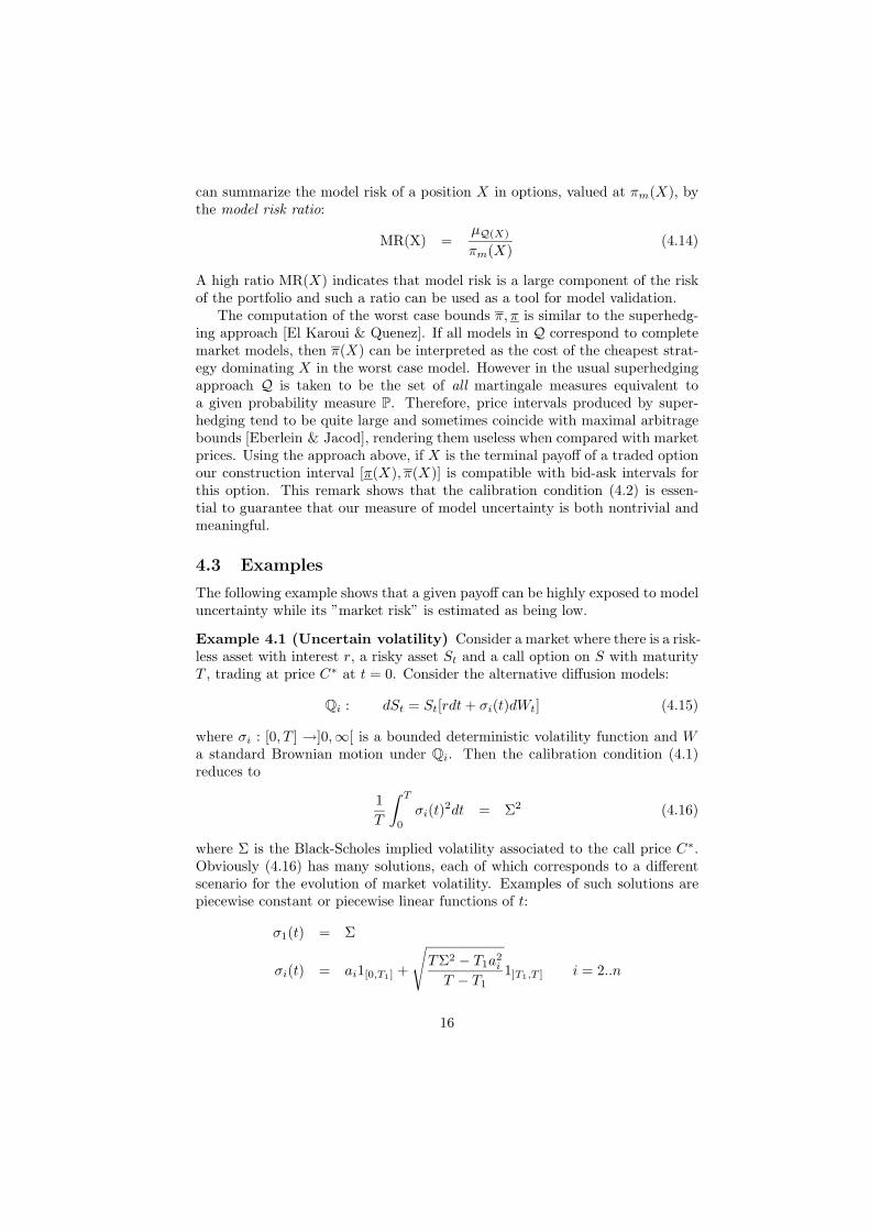
The computation of the worst case bounds π, π is similar to the superhedg-ing approach [El Karoui & Quenez]. If all models in Q correspond to completemarket models, then π(X) can be interpreted as the cost of the cheapest strat-egy dominating X in the worst case model. However in the usual superhedgingapproach Q is taken to be the set of all martingale measures equivalent toa given probability measure P. Therefore, price intervals produced by super-hedging tend to be quite large and sometimes coincide with maximal arbitragebounds [Eberlein & Jacod], rendering them useless when compared with marketprices. Using the approach above, if X is the terminal payoff of a traded optionour construction interval [π(X), π(X)] is compatible with bid-ask intervals forthis option. This remark shows that the calibration condition (4.2) is essen-tial to guarantee that our measure of model uncertainty is both nontrivial andmeaningful.

4.3 Examples

The following example shows that a given payoff can be highly exposed to modeluncertainty while its ”market risk” is estimated as being low.

Example 4.1 (Uncertain volatility) Consider a market where there is a risk-less asset with interest r, a risky asset St and a call option on S with maturityT , trading at price C∗ at t = 0. Consider the alternative diffusion models:

Qi : dSt = St[rdt + σi(t)dWt] (4.15)

where σi : [0, T ] →]0,∞[ is a bounded deterministic volatility function and Wa standard Brownian motion under Qi. Then the calibration condition (4.1)reduces to

1T

∫ T

0

σi(t)2dt = Σ2 (4.16)

where Σ is the Black-Scholes implied volatility associated to the call price C∗.Obviously (4.16) has many solutions, each of which corresponds to a differentscenario for the evolution of market volatility. Examples of such solutions arepiecewise constant or piecewise linear functions of t:

σ1(t) = Σ

σi(t) = ai1[0,T1] +

√TΣ2 − T1a2

i

T − T11]T1,T ] i = 2..n

16

with Σ < ai < Σ√

T/T1 for i = 2..n. Set a1 = Σ and let

a = maxai, i = 1..n a = minai, i = 1..n

Now consider the issue of a call option X with maturity T1 < T (with a possiblydifferent strike). For each i = 1..n, (Ω,F ,FS

t , Qi) defines a complete marketmodel (i.e. the martingale representation property holds) so under each Qi thecall can be perfectly hedged. However the corresponding ∆-hedging strategydepends on the volatility structure: it is not model–free. Therefore, while theP&L of the delta-hedged position is almost surely zero according to the modelQi used to compute the ∆, it is a random variable with non-zero variance underany Qj , j = i. In fact using the monotonicity of the Black Scholes formula withrespect to volatility it is easy to show that

π(X) = CBS(K,T1; a) π(X) = CBS(K,T1; a)

This example also shows that, when all the alternative pricing models consideredare (one dimensional) diffusion models, model uncertainty reduces to ”Vegarisk”, that is, uncertainty on volatility.

The next example shows that, conversely, a position in derivatives can havea considerable exposure to market risk but no exposure to model uncertainty:

Example 4.2 (Butterfly position) Consider a market where options are liq-uidly traded at strike levels K1 < K2 < K3, at market prices C∗

t (T,Ki), i =1, 2, 3 where K2 is at the money. A butterfly position consists in taking a shortposition in two units of the at-the-money call option Ct(T,K2) and a long po-sition in each of the calls Ct(T,K1),Ct(T,K3). This position has an exposureto “gamma” risk but since it can be synthesized using market-traded options ina model-free way the model uncertainty on its value reduces to the uncertaintyon the cost of the static hedge:

µQ(Vt) ≤ |Cbid(K1)−Cask(K1)|+|Cbid(K2)−Cask(K2)|+2|Cbid(K3)−Cask(K3)|.

A typical portfolio of derivatives will be exposed both to market risk and modeluncertainty, but the above examples illustrate the difference between the twoconcepts.

The above examples are theoretical. In the case of index options, one dis-poses of more than a hundred prices and a simple model such as (4.15) is insuf-ficient to reproduce their smile and skew features: more sophisticated modelssuch as local volatility models [Dupire (1994)], stochastic volatility models ormodels with jumps have to be used. Given an empirical data set of option prices,how can a family of pricing models compatible with market prices of optionsbe specified in an effective way? Can one implement an algorithm capable ofgenerating such a class of models verifying (4.2) and subsequently computingµ(X) for any given payoff X? [BenHamida & Cont (2004)] give an example ofsuch a procedure in the case of diffusion (”local volatility”) models:

17

5000

5500

6000

6500

7000 0

0.2

0.4

0.6

0.8

1

0.16

0.18

0.2

0.22

0.24

0.26

0.28

0.3

Maturity

Market implied volatility surface, DAX options

Strike

Impl

ied

vola

tility

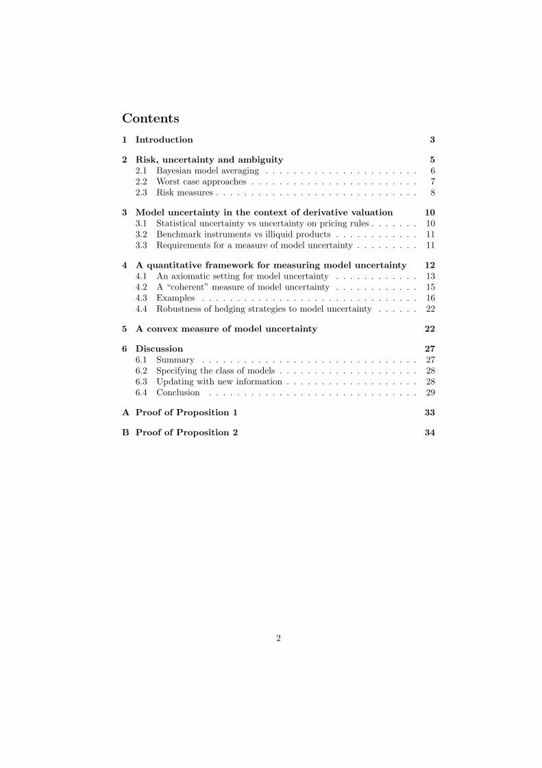
Figure 1: DAX options implied volatilities: 13 June 2001.

Example 4.3 Using an evolutionary algorithm, [BenHamida & Cont (2004)]construct a family Qi, i = 1..n of local volatility models

Qi : dSt = St[rdt + σi(t, St)dWt]

compatible with a given set of call option prices (Cbidi , Cask

i ) in the followingmanner: we start with a population of candidate solutions (σi(., .), i = 1..N)and evolve them iteratively through random search / selection cycles until theprices generated for the benchmark options by the local volatility functions(σi(., .), i = 1..N) become compatible with their bid-ask spreads. Denoting byE the set of admissible local volatility functions, this algorithm defines a Markovchain in EN , which is designed to converge to a set of model parameters whichminimize the difference between model and market prices of benchmark options.

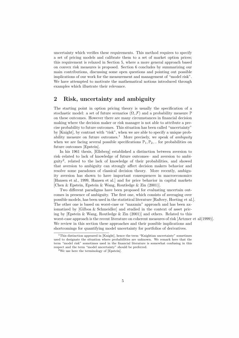
Here is an empirical example, obtained by applying this procedure to DAXindex options on June 13, 2001. The benchmark instruments are European calland put options traded on the market, numbering at around 150 quoted strikesand maturities. The implied volatility surface is depicted in figure 1. Figure2 gives examples of local volatility functions compatible with market prices ofDAX options on June 13 2001, obtained by applying the algorithm describedabove to the data: while these volatility functions look different, they are allcompatible with the market prices of quoted European call options and thiscannot be distinguished on the sole basis of market information. However, theywill not give rise to the same values for American or exotic options for whichwe face model uncertainty. Note the high level of uncertainty on short term

18

0.5

1

1.5

2

2.5 00.05

0.10.15

0.2

0.1

0.15

0.2

0.25

0.3

0.35

t

Confidence intervals for local volatility : DAX options.

S/S0

Figure 2: A family of local volatility functions σ(t, S) compatible with themarket prices of DAX options on June 13, 2001 computed using an evolutionaryalgorithm [BenHamida & Cont (2004)].

volatility, due to the fact that the value of short term options is not affectedvery much by the volatility and thus the information implied by these optionson volatility is imprecise. The diffusion models defined by these local volatilityfunctions can then be used to price a given exotic option, leading to a range ofprices.

We present now another example where market risk and model risk are bothpresent, which allows to compare the two; it also illustrates that our approachto measuring model uncertainty is not tied to the class of diffusion models andcan incorporate more general specifications:

Example 4.4 (Uncertainty on model type: local volatility vs jumps)Consider the following jump-diffusion model, used in many cases to reproduceimplied volatility skews and smiles in short term options:

Q1 : St = S0 exp[µt + σWt +Nt∑j=1

Yj ] (4.17)

where Nt is a Poisson process with intensity λ, W a standard Wiener process andYj are IID variables denoting jump sizes. In this example we choose σ = 10%,λ = 1 and the probability density of Yj is shown in Figure 3. Figure 4 showsthe implied volatilities for call options, computed using (4.17) as a model forrisk neutral dynamics.

19

−0.7 −0.6 −0.5 −0.4 −0.3 −0.2 −0.1 0 0.1 0.2 0.30

1

2

3

4

5

6

7

8

9

10

Jump size in log price0.1

0.20.3

0.40.5

0.6

90

95

100

105

1100.1

0.12

0.14

0.16

0.18

0.2

0.22

Maturity

Local volatility function

strike

Figure 3: Left: Density of jump sizes in the jump-diffusion model (4.17). Right:The local volatility, σ(t, S), as function of underlying asset and time in (4.18).

Table 1: Model uncertainty on a barrier option.Local volatility Black-Scholes+jumps µQ

At the money call T=0.2 3.5408 3.5408 0Knock out call

K=105, T=0.2, Barrier B=110 2.73 1.63 1.1

The user, uncertain whether Q1 is the right model to use, decides to pricethe option using a more familiar diffusion model

Q2 :dSt

St= rdt + σ(t, St)dWt (4.18)

where σ(t, S) is calibrated to the implied volatilities in figure (4). The resultingvolatility function σ(t, S) is shown in figure 3 (right).

These two models give exactly the same prices for all call options with matu-rities between 0.1 and 1 year and all strikes between ±10% of the money. Usingthese options as benchmark instruments, Q = Q1, Q2 verifies (4.1). However,as figure 5 shows, the typical scenarios they generate are completely different:Q1 generates discontinuous price trajectories with stationary returns while Q2

generates continuous trajectories with highly non-stationary behavior.Consider now the pricing of a barrier option, say a knock out call with strike

at the money, maturity T = 0.2 and a knock-out barrier B = 110. Due tothe high short term volatilities needed in the diffusion model to calibrate theobserved call prices, the price is higher than in the model with jumps. As shownin table 1, model uncertainty on the value of this exotic, yet quite common,derivative represents 40% of its selling price! This example clearly illustratesthat, even for common derivatives, model uncertainty does not represent a smallcorrection to the price but a major factor of risk, as important as market risk.

20

0.10.2

0.30.4

0.50.6

90

95

100

105

1100.1

0.11

0.12

0.13

0.14

0.15

0.16

0.17

0.18

Maturity

Implied volatility

Strike

Figure 4: Implied volatilities for European call and put options, produced bymodel (4.17) or (4.18).

0 0.1 0.2 0.3 0.4 0.5 0.6 0.7 0.8 0.9 190

92

94

96

98

100

102

104

106

108

t

St

0 0.1 0.2 0.3 0.4 0.5 0.6 0.7 0.8 0.9 197

98

99

100

101

102

103

104

Figure 5: Left: typical sample path of the jump-diffusion model (4.17). Right:sample path of the local volatility model (4.18). Both models give rise to thesame implied volatility skew and term structure, shown in Figure 4.

21

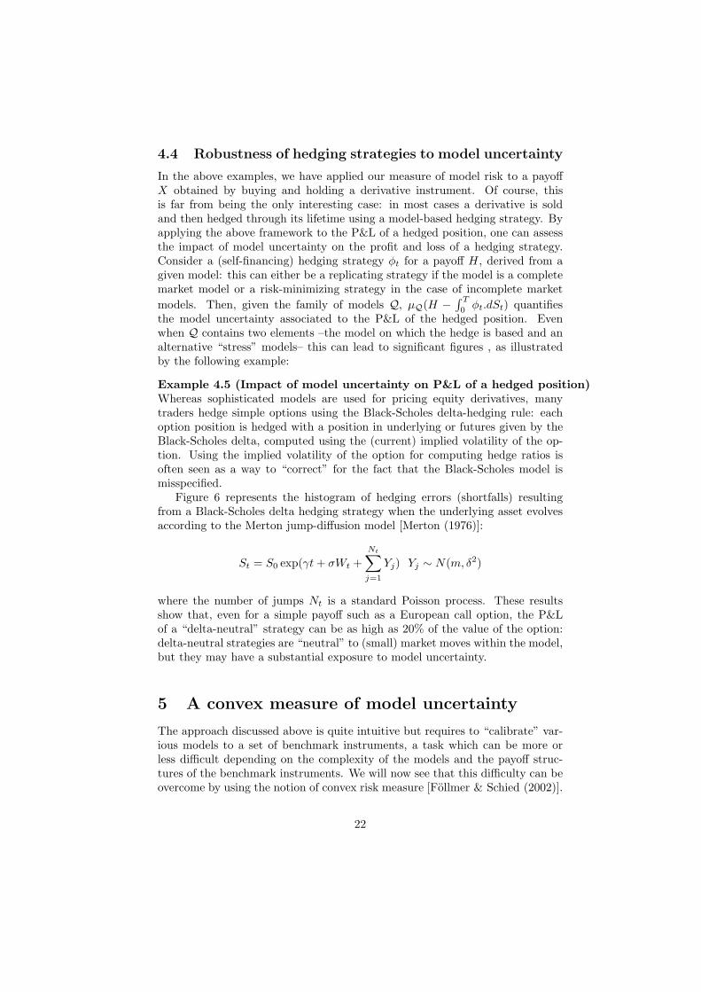
4.4 Robustness of hedging strategies to model uncertainty

In the above examples, we have applied our measure of model risk to a payoffX obtained by buying and holding a derivative instrument. Of course, thisis far from being the only interesting case: in most cases a derivative is soldand then hedged through its lifetime using a model-based hedging strategy. Byapplying the above framework to the P&L of a hedged position, one can assessthe impact of model uncertainty on the profit and loss of a hedging strategy.Consider a (self-financing) hedging strategy φt for a payoff H, derived from agiven model: this can either be a replicating strategy if the model is a completemarket model or a risk-minimizing strategy in the case of incomplete marketmodels. Then, given the family of models Q, µQ(H − ∫ T

0φt.dSt) quantifies

the model uncertainty associated to the P&L of the hedged position. Evenwhen Q contains two elements –the model on which the hedge is based and analternative “stress” models– this can lead to significant figures , as illustratedby the following example:

Example 4.5 (Impact of model uncertainty on P&L of a hedged position)Whereas sophisticated models are used for pricing equity derivatives, manytraders hedge simple options using the Black-Scholes delta-hedging rule: eachoption position is hedged with a position in underlying or futures given by theBlack-Scholes delta, computed using the (current) implied volatility of the op-tion. Using the implied volatility of the option for computing hedge ratios isoften seen as a way to “correct” for the fact that the Black-Scholes model ismisspecified.

Figure 6 represents the histogram of hedging errors (shortfalls) resultingfrom a Black-Scholes delta hedging strategy when the underlying asset evolvesaccording to the Merton jump-diffusion model [Merton (1976)]:

St = S0 exp(γt + σWt +Nt∑j=1

Yj) Yj ∼ N(m, δ2)

where the number of jumps Nt is a standard Poisson process. These resultsshow that, even for a simple payoff such as a European call option, the P&Lof a “delta-neutral” strategy can be as high as 20% of the value of the option:delta-neutral strategies are “neutral” to (small) market moves within the model,but they may have a substantial exposure to model uncertainty.

5 A convex measure of model uncertainty

The approach discussed above is quite intuitive but requires to “calibrate” var-ious models to a set of benchmark instruments, a task which can be more orless difficult depending on the complexity of the models and the payoff struc-tures of the benchmark instruments. We will now see that this difficulty can beovercome by using the notion of convex risk measure [Follmer & Schied (2002)].

22

−140 −120 −100 −80 −60 −40 −20 0 20 40 600

1

2

3

4

5

6

Figure 6: Distribution of P&L of a Black-Scholes delta-neutral hedge for aEuropean at-the-money 1 year call, expressed as a percentage of the optionprice at inception. One of the curves corresponds to a delta computed usingthe implied volatility at t = 0, the other curve corresponds to daily updating ofimplied volatility.

23

As noted in Section 2.3, a convex risk measure can be represented in the form(2.10), where the penalty function α is a rather abstract object whose value doesnot have a clear financial interpretation. Also, the representation (2.10) lacksa normalization which could allow to compare it to marked-to-market valuesof portfolios. We show here that a special choice of the penalty function canresolve these issues and provide us simultaneously with a suitable generalizationof (4.12) .

Consider as in Section 4, a family of pricing rules Q and a set of benchmarkoptions with payoffs (Hi)i∈I with market prices (C∗

i )i∈I . However, instead ofrequiring the pricing models Q ∈ Q to reproduce the market prices of benchmarkinstruments exactly as in (4.1) or within bid-ask spreads as in (4.2), we considera larger class of pricing models, not necessarily calibrated to observed optionprices, but penalize each model price by its pricing error ‖C∗ − EQ[H]‖ on thebenchmark instruments:

π∗(X) = supQ∈Q

EQ[X] − ‖C∗ − EQ[H]‖ (5.1)

π∗(X) = −π∗(−X) = infQ∈Q

EQ[X] + ‖C∗ − EQ[H]‖ (5.2)

This means we price the payoff X with all the pricing models Q ∈ Q butwe take more or less seriously the prices produced by any of the pricing modelsaccording to the precision with which they are capable of reproducing the marketprices of benchmark instruments. Different choices of norms for the vector(C∗

i − EQ[Hi])i∈I lead to different measures for the “calibration error”:

‖C∗ − EQ[H]‖∞ = supi∈I

|C∗i − EQ[Hi] | (5.3)

‖C∗ − EQ[H]‖1 =∑i∈I

|C∗i − EQ[Hi] | (5.4)

or, more generally : ‖C∗ − EQ[H]‖p = [∑i∈I

|C∗i − EQ[Hi] |p]1/p (5.5)

In the language of [Follmer & Schied (2002)], ρ(X) = π∗(−X) is a convex riskmeasure associated with the penalty function α given by

α(Q) = ‖C∗ − EQ[H]‖ if Q ∈ Q= +∞ if Q /∈ Q

Define now, by analogy with (4.12), the following measure for model uncertainty:

∀X ∈ C, µ∗(X) = π∗(X) − π∗(X) (5.6)

The following result shows that µ∗ defines a measure of model uncertainty withthe required properties:

Proposition 2 If the pricing error ‖C∗ − EQ[H]‖ verifies:

∀Q ∈ Q, ∀i ∈ I, ‖C∗ − EQ[H]‖ ≥ |C∗i − EQ[Hi] | (5.7)

then the following properties hold for π∗, π∗ and µ∗:

24

1. π∗ assigns to any benchmark option a value lower than its market price:

∀i ∈ I, π∗(Hi) ≤ C∗i (5.8)

π∗ assigns to any benchmark option a value higher than its market price:

∀i ∈ I, π∗(Hi) ≥ C∗i (5.9)

2. Assume the class of pricing models contains at least one model compatiblewith the market prices of the benchmark options:

∃Q ∈ Q, ∀i ∈ I, EQ[ Hi ] = C∗i . (5.10)

Then ∀i ∈ I, π∗(Hi) = π∗(Hi) = C∗i and for any payoff X ∈ C, π∗(X) ≥

π∗(X).

3. Under assumption (5.10), µ∗ defined by (5.6) is a measure of model un-certainty verifying the properties (4.4)-(4.5)-(4.6)-(4.7).

4. Static hedging reduces model uncertainty: under assumption (5.10), di-versifying a position using long positions in benchmark derivatives reducesmodel uncertainty:

[ 1 ≥ λk ≥ 0,

K∑k=0

λk = 1] ⇒ µ∗(λ0X +K∑

k=1

λkHk) ≤ µ∗(X) (5.11)

In particular, any position which can be replicated by a convex combinationof available derivatives has no model uncertainty:

[∃(λi)i∈I , 1 ≥ λi ≥ 0,∑i∈I

λi = 1,X =∑i∈I

λiHi] ⇒ µ∗(X) ≤ 0. (5.12)

Proof: see Appendix.

Remark 5.1 (Penalization by weighted pricing error) More generally onecould consider weighted pricing errors as penalty function, for instance:

‖C∗ − EQ[H]‖1,w =∑i∈I

wi|C∗i − EQ[Hi] |.

However, it is interesting to note that requiring (5.8)–(5.9) for any specificationof Q implies that wi ≥ 1. Therefore the penalty functions (5.3)–(5.4)–(5.5) arethe “minimal” ones verifying our requirements. Since putting a weight on thei-th option amounts to changing its nominal, Hi should be interpreted as thepayoff of i-th benchmark option, the nominal being determined by the (maximal)quantity of the i-th option available to the investor.6

6See [Cont & Gabay] for a discussion of this point.

25

Remark 5.2 Properties (5.11)-(5.12) replace properties (4.8)-(4.9) verified bythe coherent measure of model uncertainty µQ: this is due to the fact that aconvex measure of risk cannot extrapolate the risk of a portfolio to a larger, pro-portional portfolio. A closer look at (5.12) shows that it is the only reasonabledefinition of a static hedge: in line with remark 5.1, Hi represents, in nominalterms, the maximal position in the i-th derivative so feasible positions in thisderivative are of the type λi Hi with 0 ≤ λi ≤ 1. By contrast in (4.8)-(4.9) weimplicitly allowed unlimited short and long positions in all derivatives and Hi

was defined up to a constant.

In practice µ∗ can be computed in the following manner. Given a set of prices forthe benchmark options, we first choose a pricing model Q1 which can reproducethese prices and is easily calibrated to option prices. Typical examples are onedimensional diffusion models (local volatility models) used for equity and indexderivatives and the SABR model [Hagan et al., 2002] for European options oninterest rates. Such models are typically used for their ability to calibrate marketprices, so they satisfy (5.10) but may not generate realistic dynamics for futuremarket scenarios. We have then the freedom to add to such a calibrated modelQ1 other pricing models Q2, Q3, ... with more realistic features but which may bemore complex to calibrate. The procedure above does not require to calibratethese models precisely but simply to penalize their pricing errors: the easy-to-calibrate model Q1 anchors our measure of model uncertainty in the marketprices while more realistic models Q2, Q3, ... can be incorporated without havingto set up heavy numerical procedures for their calibration.

Remark 5.3 (Bid ask spreads) The above construction can be generalizedto the case where market values of benchmark options are not unique but givenby bid and ask prices Cbid

i , Caski . The condition (5.7) then has to be replaced

by:α(Q) ≥ sup

i∈Imax((EQ[Hi] − Cbid

i )+, (Caski − EQ[Hi])+).

Remark 5.4 The constraint (5.10) of including at least one arbitrage-free pric-ing rule Q0 ∈ Q which calibrates the market prices guarantees that option pricesare arbitrage-free and amounts to requiring that ρ(0) = 0 (see the proof ofProposition 2), which is the normalization condition proposed in [Follmer & Schied (2002)].However, this condition may be difficult to satisfy in some cases, especially inpresence of many benchmark instruments with different payoff structures: avail-able models may only be able to reproduce all options to within a certain pre-cision ε > 0. In this case one can still conserve the structure above by replacingπ∗ by π∗ + ε, π∗ by π∗ − ε and µ∗ by µ∗ + 2ε. This point is further developedin [Cont & Gabay].

As more liquid instruments become available, this has the effect of increasingπ∗ and of decreasing π∗ thus the measure of model uncertainty becomes smaller.This can be interpreted in the following way: the addition of more liquid optionsallows a wider range of model-free (static) hedging strategies which allow toreduce exposure to model uncertainty on a given portfolio.

26

Also, from the expression of the penalty functions (5.3)–(5.4)–(5.5) it isclear that models with lower pricing errors will be more and more favored asthe number of benchmark instruments |I| increases. As |I| → ∞, ‖C∗−EQ[H]‖will stay finite only if the calibration error is bounded independently of |I|; thishappens for instance if the pricing model Q misprices only a finite number ofbenchmark options, all others being calibrated. Conversely, when there are nooptions available (I = ∅), ρ is a coherent risk measure defined by the set Q.

6 Discussion

We now summarize the main contributions of this work, discuss some openquestions and possible implications for the risk management of derivative in-struments.

6.1 Summary

We have proposed a quantitative framework for measuring the impact of modeluncertainty on derivative pricing. Starting from a set of traded benchmark op-tions and a family Q of option pricing models, we associate a measure of modeluncertainty µ(X), expressed in monetary units, with any derivative with payoffX in two ways. The first method (Section 4) requires the models in Q to bepricing models calibrated to the benchmark options and computes the rangeµQ(X) of prices for X over all of these calibrated models. The second method(Section 5) does not require any calibration but penalizes a model price by itspricing error on the benchmark instruments. In both cases, the specification ofa set of benchmark instruments constitutes a key ingredient in our procedure,which was missing in preceding approaches to model risk: without it, the mea-sures of model risk may range between zero and infinity and be meaninglesswhen compared to market values of portfolios.

Both of these approaches verify the intuitive requirements, outlined in Sec-tion 3, that a measure of model uncertainty should have in order to be meaning-ful in the context of risk management. They are both compatible with marketvalues of traded options and take into account the possibility of model-free hedg-ing with options. They lead to a decomposition of the risk of a position intothe sum of a first term, which is of the same order of magnitude as its nominalvalue and a second term, which can be interpreted as a component of the bid-askspread due to model uncertainty. Measures of model uncertainty computed inthis manner are realistic enough to be considered as bid-ask values. They aredirectly comparable with market prices and common measures of market risk.

Our approach does not require the set of pricing models considered to de-fine equivalent measures on scenarios. When all the models considered areone dimensional diffusions, model uncertainty reduces to uncertainty on futurevolatility and the approach adopted here is similar to the Lagrangian UncertainVolatility model of [Avellaneda & Paras]. But the notion of model uncertaintyproposed here reaches beyond the concept of uncertain volatility and can en-

27

compass other types of models (jumps, stochastic volatility) or sources of modeluncertainty (number of factors in multifactor models, jump sizes, ..).

Finally, it is important to note that our measures of model risk are notdefined “up to a normalization constant”: they directly produce numbers con-sistent with mark-to-market valuation of portfolios, when available, and do notrequire an ad-hoc scaling factor in order to be meaningfully used to provisionfor model risk.

6.2 Specifying the class of models

The relevance of our measure of model risk partly hinges on the specification ofthe class Q of models. As noted by [Hansen & Sargent], “the development ofcomputationally tractable tools for exploring model misspecification [...] shouldfocus on what are the interesting classes of candidate models for applications”.This issue seems less difficult in option pricing than, say, in macroeconomics,since a market consensus has emerged on a set of standard pricing models(though not a unique model!) for each type of underlying asset in the lastdecade.

In the approach described in Section 4, a further requirement is the abilityto calibrate the models to market observations. Standard model calibrationalgorithms yield a single solution/ pricing model. A first way out is to specifydifferent model classes and perform calibration separately in each model class,yielding a calibrated set of parameters from each class. This approach takes intoaccount uncertainty on model type. Another approach, an example of whichwas given in Example 4.3, is to consider a single model class but recognize thatthe calibration problem may have multiple solutions and use a stochastic searchalgorithm [BenHamida & Cont (2004)]. The two approaches are not exclusiveand may be combined. The availability of efficient numerical procedures willultimately orient market practice in one direction or the other.

The approach of Section 5, based on convex risk measures, has the advantageof relaxing this calibration requirement and thus is potentially more flexiblefrom a computational point of view. The advantages and drawbacks of the twoapproaches remain to be studied in specific settings.

6.3 Updating with new information

In the above discussion, we have considered a market viewed at time t = 0. Howdoes the procedure described above apply as time evolves? By analogy with(4.12), one could define a dynamic bid-ask interval by replacing expectations byconditional expectations:

πt(X) = ess supQ∈Q

EQ[X|FSt ] πt(X) = ess inf

Q∈QEQ[X|FS

t ] (6.1)

Then, for each t, πt and πt define coherent risk measures that make use ofthe information on the evolution of the underlying up to time t and a naturalcandidate for building a measure of model uncertainty would then be µt(X) =

28

πt(X) − πt(X). However there are at least two objections to the formulation(6.1). The first objection is that it does not guarantee dynamic consistency(i.e. a dynamic programming principle). This problem has been studied inthe framework of a Brownian filtration in [Chen & Epstein, Peng] where it isshown that a special structure has to be imposed on Q in order for dynamicconsistency to hold. These authors examine the case where the family Q0 iskept fixed while the market evolves through the evolution of the asset price.However the pricing models Q ∈ Q0 have only been calibrated to the value ofthe benchmark options at t = 0 and simply conditioning them on the evolutionof the underlying asset clearly does not exploit the information given by theevolution of the market prices of the benchmark options. This is due to thefact that, in a realistic framework, one cannot assume that the “true” modeldescribing the joint evolution of the benchmark derivatives is included in theset Q0. In line with this remark, the market practice is to re-calibrate pricingmodels as prices of options evolve through time. This re-calibration procedureimplies that the set of pricing rules Q0 cannot be used at a later date but hasto be replaced by a set Q(t) of pricing rules verifying:

∀Q ∈ Q(t),∀ i ∈ I, EQ[Hi] ∈ [Cbidi (t), Cask

i (t)] (6.2)

This leads to a time-dependent set Q(t) consisting of updated versions Q(t)of elements of Q0, each defining a risk-neutral measure on the future pathsD([t, T ]) verifying (6.2). In other words, since the result of model calibrationprocedure at time t depends on the prices of benchmark instruments (C∗

i (t), i ∈I), Q(t) is a set of random measures, whose evolution depends on the marketprices of benchmark options. Hence the updating procedure implied by re-calibration procedures is more subtle than conditioning on the past evolution ofthe underlying asset: the updating procedure must also reflect the evolution ofprices in the options market.

A related practical question is that of sensitivity of measures of model un-certainty to market conditions.7 This question is already present in the caseof market risk measures such as VaR, which can fluctuate in a non-negligiblemanner as market conditions (e.g. prices of underlying assets) vary. A strongsensitivity would blur the distinction between market risk and model uncer-tainty. Case studies remain to be done in order to clarify the impact of thissensitivity in practical examples of derivatives portfolios.

6.4 Conclusion

Quantitative risk management took off in the 1990s with the availability of sim-ple tools such as Value-at-Risk for measuring market risk: notwithstanding itstechnical imperfections, Value-at-Risk convinced practitioners that it is possiblein practice to quantify market risk, had a great impact on risk management prac-tices and motivated many researchers to improve this methodology in variousways.

7We thank Joel Bessis for pointing out this issue.

29

In the recent years, various case studies have indicated the importance of“model risk” in the derivative industry and some spectacular failures in riskmanagement of derivatives have emphasized the consequences of neglectingmodel uncertainty. Many large financial institutions are conscious of this is-sue and have been developing methods to tackle it systematically.

We have provided in this paper a simple methodology which can be usedto quantify model uncertainty and provides meaningful figures compatible withmark-to-market values of portfolios, when they are available. Our approach canserve as a basis for provisioning for model uncertainty or simply as a decisionaid for risk managers and regulators.

We hope this work will stimulate further case studies using the methodologypresented here, in order to better understand the impact of model uncertaintyin various contexts.

References

[Allen & Padovani] Allen, S. and Padovani, O. (2002) Risk management usingquasi-static hedging, Economic Notes, 31(2), 277–236.

[Artzner et al(1999)] Artzner P., Delbaen F., Eber J.M., Heath D. (1999) Co-herent measures of risk, Mathematical Finance, 9, No. 3, 203–228.

[Avellaneda et al] Avellaneda M., Levy A. & Paras, A. (1995): Pricing andhedging derivative securities in markets with uncertain volatilities, AppliedMathematical Finance, 2, 73-88.

[Avellaneda & Paras] Avellaneda, M. & Paras, A. (1996): Managing theVolatility Risk of Portfolios of Derivative Securities: the Lagrangian Uncer-tain Volatility Model, Applied Mathematical Finance, 3, 31–52.

[BenHamida & Cont (2004)] Ben Hamida, S. & Cont, R. (2004) Recoveringvolatility from option prices by evolutionary optimization, Rapport InterneCMAP No 534, Ecole Polytechnique.

[Buff] Buff, R. (2001) Uncertain volatility models, Springer Finance.

[Carr et al.] Carr P., Geman H., Madan, D.B. (2001) Pricing and hedging inincomplete markets, Journal of Financial Economics, Vol. 62, 131-167.

[Chen & Epstein] Chen, Z. & Epstein, L.G. (2002) Ambiguity, risk and assetreturns in continuous time, Econometrica, Vol. 70, 4, 1403–1443.

[Crouhy et al.] Crouhy, M., Galai, D. & Mark, R. (1998) Model Risk, Journalof Financial Engineering, Vol. 7 No. 3/4, pp. 267– 288.

[Cont & Gabay] Cont, R. & Gabay, D. (2005) Model risk: a convex dualityapproach, Working Paper.

30

[Delbaen & Schachermayer] Delbaen, F. & Schachermayer, W. (1998) The fun-damental theorem of asset pricing for unbounded stochastic processes, Math.Ann., 312(2):215–250, 1998.

[Doleans-Dade (1971)] Doleans-Dade, C. (1971) Integrales stochastiques parrapport a une famille de probabilites, in: Seminaire de Probabilites V, LectureNotes in mathematics Vol. 191, 141–146, Berlin: Springer.

[Dupire (1994)] Dupire, B. (1994) Pricing with a smile, RISK, 7 (1), 18–20.

[Eberlein & Jacod] Eberlein, E. and Jacod, J. (1997) On the range of optionprices, Finance and Stochastics, 1, 131–140.

[Ellsberg] Ellsberg, D. (1961) Risk, Ambiguity, and the Savage Axioms, Quar-terly Journal of Economics, 75, 643-669.

[Elliott (1997)] Elliott, M. (1997) Controlling Model Risk, Derivatives Strategy,June.

[El Karoui et al (1998)] El Karoui, N., Jeanblanc, M. and S. Shreve (1998) Ro-bustness of the Black and Scholes Formula, Mathematical finance, 8, 93–126.

[El Karoui & Quenez] El Karoui, N. & Quenez, M.C. (1995) Dynamic program-ming and the pricing of contingent claims in incomplete markets, SIAM Jour-nal of Control and Optimization, Vol 33, No 1, 29–66.

[El Karoui & Rouge] El Karoui, N. & Rouge, R. (2000) Pricing via utility max-imization and entropy, Mathematical Finance, 10, 259–276.

[Epstein] Epstein, L.G. (1999) A definition of uncertainty aversion, Review ofEconomic Studies, 65, 579–608.

[Epstein & Wang] Epstein, L.G. & Wang, L.(1995) Uncertainty, risk neutralmeasures and asset price booms and crashes, Journal of Economic Theory,67, 40–80.

[Follmer & Schied (2002)] Follmer, H. & Schied, A. (2002) Convex measures ofrisk and trading constraints, Finance and Stochastics, 6, No. 4, 429-447.

[Follmer & Schied (2002b)] Follmer, H. & Schied, A. (2002) Stochastic Finance,Walter de Gruyter.

[Frittelli & Gianin (2002)] Frittelli, M. & Gianin, E.R. (2002) Putting order inrisk measures, Journal of Banking and Finance, Volume 26, Issue 7, Pages1247-1561.

[Gilboa & Schmeidler] Gilboa & Schmeidler (1989) Maxmin expected utilitywith non-unique prior, Journal of mathematical economics, 18, 141-153.

[Gundel] Gundel, A. (2004) Robust utility maximization for complete and in-complete market models, forthcoming in: Finance and Stochastics.

31

[Hagan et al., 2002] Hagan P., Kumar D., Lesniewski A., Woodward D. (2002)Managing smile risk, Wilmott Magazine.

[Hansen et al., 1999] Hansen L., Sargent Th., Tallarini T. (1999) Robust per-manent income and pricing, Review of Economic Studies, 66, 872–907.

[Hansen & Sargent] Hansen, L. & Sargent, Th. (2001) Time inconsistency ofrobust control, Working paper.

[Hansen et al.] Hansen L., Sargent Th., Turluhambetova G.A., Williams N.(2002) Robustness and uncertainty aversion, Working Paper.

[Hoeting et al.] Hoeting J.A., Madigan D., Raftery A.E., Volinsky C.T. (1999)Bayesian model averaging: a tutorial, Statistical Science, 14, 4, 382–417.

[Jacquier & Jarrow (2000)] Jacquier, E. & Jarrow, R. (2000): Bayesian analysisof contingent claim model error, Journal of Econometrics, Vol. 94, 145–180.

[Kabanov] Kabanov, Yuri (2001) Arbitrage theory, in: Jouini et al (eds.): Op-tion pricing, interest rates and risk management, Cambridge University Press.

[Karatzas & Zamfirescu] Karatzas, I. and Zamfirescu, I.M. (2004) Optimal stoing with model uncertainty, Working Paper.

[Kerkhof et al.] Kerkhof J., Melenberg B. and Schumacher, H. (2002) Modelrisk and regulatory capital, Working Paper.

[Knight] Knight, F. (1921) Risk, uncertainty and profit, Boston: Houghton Mif-flin.

[Lyons] Lyons, T.J. (1995) Uncertain volatility and the risk free synthesis ofderivatives, Applied mathematical finance, 2, 117–133.

[Lyons & Smith] Lyons, T.J. & Smith, A.T. (1999) Uncertain volatility, RISK,September, 106–109.

[Merton (1976)] Merton, R.C. (1976) Option Pricing When Underlying StockReturns Are Discontinuous, Journal of Financial Economics, 3, 125–144.

[Peng] Peng, S. (2004) Nonlinear expectations and dynamic risk measures,in: Stochastic methods in finance, Lecture Notes in Mathematics Vol. 1856,Springer, pp. 165–254.

[Raftery] Raftery, A. E. (1993) Bayesian model selection in structural equationmodels. In: K. Bollen and J. Long (eds.): Testing Structural Equation Models,163180, Sage, Newbury Park, CA.

[Routledge & Zin (2001)] Routledge, B.R. & Zin, S. (2001) Model uncertaintyand liquidity, NBER Working Paper 8683.

[Savage] Savage, L.J. (1954) The foundations of statistics, Wiley.

32

[Schied] Schied, A. (2004) Optimal investments for robust utility functionals incomplete market models. To appear in Math. Oper. Research.

[Williams (1999)] Williams, D. (1999) Models vs. The Market: Survival of theFittest, Report FIN514, Meridien Research.

A Proof of Proposition 1

1. Each Q ∈ Q verifies the calibration condition (4.2). By taking supremum(resp. infimum) over Q ∈ Q we obtain: Cask

i ≥ π(Hi) ≥ π(Hi) ≥ Cbidi .

2. (4.4) follows from the above inequality. To show (4.5), note that for anyφ ∈ S and any Q ∈ Q the gains process Gt(φ) is a Q-martingale so EQ[X+∫ T

0φt.dSt] = EQ[X] so π(X +

∫ T

0φt.dSt) = π(X) and π(X +

∫ T

0φt.dSt) =

π(X) so µQ(X+∫ T

0φt.dSt) = µQ(X). Choosing in particular X = x0 ∈ R

we obtain (4.6).To show the convexity property (4.7), consider X,Y ∈ C and λ ∈ [0, 1].For each Q ∈ Q we have

λ infQ∈Q

EQ[X] + (1 − λ) infQ∈Q

EQ[Y ] ≤ EQ[λX + (1 − λ)Y ]

≤ λ supQ∈Q

EQ[X] + (1 − λ) supQ∈Q

EQ[Y ]

By taking supremum (resp. infimum) over Q we obtain:

λπ(X) + (1 − λ)π(Y ) ≤ π(λX + (1 − λ)Y )≤ π(λX + (1 − λ)Y ) ≤ λπ(X) + (1 − λ)π(Y )

from which (4.7) is easily derived.Let us now show (4.8). Consider a portfolio composed of a long position inX, and positions ui, i = 1..k in k benchmark options Hi, i = 1..k. Assumewithout loss of generality that the first u1, ..., uk1 are long positions, theothers being short positions. Since any Q ∈ Q verifies (4.2), we have:

EQ[X] +k1∑

i=1

uiCbidi +

k∑i=k1+1

uiCaski ≤ EQ[X +

k∑i=1

uiHi]

≤ EQ[X] +k1∑

i=1

uiCaski +

k∑i=k1+1

uiCbidi

By taking the supremum (resp. the infimum) over Q ∈ Q we obtain:

π(X) +k1∑

i=1

uiCbidi +

k∑i=k1+1

uiCaski ≤ π(X +

k∑i=1

uiHi)

π(X +k∑

i=1

uiHi) ≤ π(X) +k1∑

i=1

uiCaski +

k∑i=k1+1

uiCbidi

33

Adding the last two inequalities and taking into account the signs of ui

we obtain:

π(X +k∑

i=1

uiHi) − π(X +k∑

i=1

uiHi) ≤ π(X) − π(X) +k∑

i=1

|ui(Cbidi − Cask

i )|

which yields (4.8). Substituting X = 0 yields (4.9).

B Proof of Proposition 2

Let π∗, π∗ and µ∗ be defined by (5.1)-(5.2)-(5.6).

1. Using (5.7) and noting that

∀Q ∈ Q,∀i ∈ I, −|C∗i − EQHi| ≤ C∗

i − EQ[Hi] we obtain

EQHi − ‖C∗ − EQ[H]‖ ≤ EQHi − |C∗i − EQHi|

≤ EQ[Hi] + C∗i − EQ[Hi] = C∗

i

Taking the supremum over Q ∈ Q we obtain π∗(Hi) ≤ C∗i . Similarly,

starting from

∀Q ∈ Q,∀i ∈ I, |C∗i − EQHi| ≥ C∗

i − EQ[Hi] we obtain

EQ[Hi] + ‖C∗ − EQ(H)‖ ≥ EQ[Hi] + |C∗i − EQHi|

≥ EQ[Hi] + C∗i − EQ[Hi] = C∗

i

Taking the infimum over Q ∈ Q we obtain π∗(Hi) ≥ C∗i .

2. Since ρ defined by ρ(X) = π∗(−X) is a convex risk measure, applying(2.9) to Y = −X and λ = 1/2 yields:

ρ(0) = ρ(−X

2+

X

2) ≤ 1

2(ρ(X) + ρ(−X))

Since π∗(X) = ρ(−X) and π∗(X) = −ρ(X) we obtain

∀X ∈ C, π∗(X) ≥ π∗(X) + 2ρ(0)

Now remark that −ρ(0) = infQ∈Q ‖C∗ − EQ[H]‖ is simply the smallestcalibration error achievable using any of the pricing models in Q. If weassume the class of pricing models contains at least one model compatiblewith the market prices of the benchmark options:

∃Q ∈ Q, ∀i ∈ I, EQ[ Hi ] = C∗i .

then ρ(0) = 0 and we obtain ∀X ∈ C, π∗(X) ≥ π∗(X).

34

3. From the above inequality π∗(Hi) ≥ π∗(Hi) with (5.8) and (5.9) we obtain:

∀i ∈ I, C∗i ≥ π∗(Hi) ≥ π∗(Hi) ≥ C∗

i

hence µ∗(Hi) = 0 for all i ∈ I. To show (4.6), note that for any φ ∈ Sand any Q ∈ Q the gains process Gt(φ) is a Q-martingale so EQ[X] =x0 + EQ[

∫ T

0φ.dS] = x0. Therefore ρ(X) = −x0 and π∗(X) = π∗(X) = x0

hence µ∗(X) = 0. More generally,

ρ(X +∫ T

0

φtdSt) = supQ

EQ[−X −∫ T

0

φtdSt] − ‖C∗ − EQ[H]‖

= supQ

EQ[−X] − ‖C∗ − EQ[H]‖

since∫ t

0φ.dS is a martingale under each Q ∈ Q, which implies (4.5).

Using the convexity property (2.9) of ρ we have, for any X,Y ∈ C andλ ∈ [0, 1]:

µ∗(λX + (1 − λ)Y ) = ρ(λX + (1 − λ)Y ) + ρ(−λX − (1 − λ)Y )≤ λρ(X) + (1 − λ)ρ(Y ) + λρ(−X) + (1 − λ)ρ(−Y )= λ[ρ(X) + ρ(−X)] + (1 − λ)[ρ(Y ) + ρ(−Y )]= λµ∗(X) + (1 − λ)µ∗(Y )

which shows the convexity property (4.7) for µ.

4. To show (5.11), consider λk ≥ 0, k = 0..K with∑K

k=0 λk = 1. Using theconvexity of µ∗

µ∗(λ0X +K∑

k=1

λkHk) ≤ λ0µ∗(X) +K∑

k=1

λkµ∗(Hk)

As shown above, µ∗(Hi) = 0 for all i ∈ I and 0 ≤ λ0 ≤ 1 we obtain (5.11).Choosing X = 0 and noting that µ∗(0) = 0, we obtain (5.12).

35