Embed Size (px)
Citation preview

Purdue UniversityPurdue e-PubsInternational Refrigeration and Air ConditioningConference School of Mechanical Engineering
2014
Model Predictive Control of Variable RefrigerantFlow SystemsNeera JainMitsubishi Electric Research Labs, United States of America, [email protected]
Daniel J. BurnsMitsubishi Electric Research Labs, United States of America, [email protected]
Stefano Di CairanoMitsubishi Electric Research Labs, United States of America, [email protected]
Christopher R. LaughmanMitsubishi Electric Research Labs, United States of America, [email protected]
Scott A. BortoffMitsubishi Electric Research Labs, United States of America, [email protected]
Follow this and additional works at: http://docs.lib.purdue.edu/iracc
This document has been made available through Purdue e-Pubs, a service of the Purdue University Libraries. Please contact [email protected] foradditional information.Complete proceedings may be acquired in print and on CD-ROM directly from the Ray W. Herrick Laboratories at https://engineering.purdue.edu/Herrick/Events/orderlit.html
Jain, Neera; Burns, Daniel J.; Di Cairano, Stefano; Laughman, Christopher R.; and Bortoff, Scott A., "Model Predictive Control ofVariable Refrigerant Flow Systems" (2014). International Refrigeration and Air Conditioning Conference. Paper 1545.http://docs.lib.purdue.edu/iracc/1545

2613, Page 1
Model Predictive Control of Vapor Compression Systems
Neera JAIN, Daniel J. BURNS*, Stefano DI CAIRANO, Christopher R. LAUGHMAN, Scott A.BORTOFF
Mitsubishi Electric Research Laboratories,Cambridge, MA, [email protected]
* Corresponding Author
ABSTRACT
Model Predictive Control (MPC) of vapor compression systems (VCSs) offers several advantages over conventionalcontrol methods (such as multivariable process control with selector logic) in terms of 1) the resulting closed-loopperformance and 2) the control engineering design process. VCSs are multivariable systems and feature constraintson system variables and actuators that must be enforced during steady-state and transient operation. We present thedesign and validation of an MPC for a split ductless VCS. The design regulates room temperature with zero steadystate error for unknown changes in the thermal load and enforces constraints on system variables such as compressordischarge temperature and actuator ranges and rates. We show how the MPC design can evolve during the engineeringprocess by adding and modifying constraints and process variables. The design methodology provides guaranteesin terms of closed loop stability and convergence. Importantly, in contrast to other published results on MPC forVCSs, our design makes use of only available temperature measurements and does not require pressure or mass flowmeasurements which are typically not available in production VCSs.
1. INTRODUCTION
Model Predictive Control (MPC) (Garcia et al., 1989) of vapor compression systems (VCSs) offers several advantagesover conventional control methods (such as multivariable process control with selector logic) in terms of 1) the re-sulting closed-loop performance and 2) the control engineering design process. VCSs are multivariable systems andfeature constraints on system variables and actuators that must be enforced during steady-state and transient operation.Control requirements typically include regulation of process variables such as room temperatures, high bandwidthtransient response for rapid pull down, constraint enforcement during transient and steady-state operation, and optimalsteady-state energy efficiency. Conventional methods of control use classical or multivariable process control theory tomeet the requirements associated with regulation, transient response, and steady-state efficiency, together with selectorlogic designed to prioritize the process variables in order to enforce constraints (Amano, 2012). However, for multi-variable systems with more than one constraint, the interactions among the selector logic make it difficult to designand validate the feedback controller; feedback gains are often detuned resulting in a conservative feedback controllerthat is intended to stay away from the constraints. At best, this results in slow transient response and poor rejection ofdisturbances and at worst, in a controller that is unable to maintain the system within the constraints.
In contrast, MPC is a technology that is well suited to the requirements of VCS control. Elliott and Rasmussen (2008)and Koeln and Alleyne (2013) investigate decentralized MPC for multi-evaporator VCSs to regulate evaporator super-heat and cooling capacity while mitigating coupling between individual evaporators. However, evaporator superheatand cooling capacity are feedback variables that may require pressure or mass flow measurements which are typicallynot available in production VRF systems. To overcome model uncertainty between a linear MPC and the nonlinearVCS, Wallace et al. (2012) use a state estimator with an input disturbance model that results in zero steady-state reg-ulation error. Heuristic tuning guidelines are provided for the input disturbance model. Like Elliott and Rasmussen(2008), Wallace et al. (2012) use MPC to control the cooling capacity of the VCS, while a supervisory controller isused to determine appropriate setpoints to regulate zone temperature(s).
15th International Refrigeration and Air Conditioning Conference at Purdue, July 14-17, 2014
2613, Page 2
However, when considering zone temperature rather than cooling capacity as a feedback variable, the unknown andunmeasurable thermal loads on the VCS are disturbances that must be rejected by the MPC. Our approach is toformulate the state estimator in such a way that the effect of disturbances are lumped into auxiliary output disturbancestates, thereby eliminating the need to measure the thermal load. This approach has the added benefit of offset-freeestimation (Pannocchia and Rawlings, 2003; Maeder et al., 2009) of all measured outputs. This means that our closed-loop system will achieve zero steady-state error between set point variables and regulated variables for constant butunmeasured and unknown values of the thermal load disturbance. Moreover, we show that MPC offers a flexibleand systematic design process in which the constraints, for example, can be modified as the design evolves, and theresulting controller can be computed and analyzed immediately, providing rigorous guarantees on optimality, transientperformance, and stability.
The paper is organized as follows. Section 2 describes the nonlinear model of a single zone split ductless vaporcompression system and its linearization for controller design. The design of the MPC is presented in Section 3 andsimulation results showing the performance and capabilities of the controller are presented and discussed in Section 4.Concluding remarks are offered in Section 5.
2. SYSTEM MODELING
A nonlinear dynamic model of a 2.6 kW capacity split ductless VCS is developed using the THERMOSYS Toolboxfor MATLAB/Simulink (Alleyne, 2012). THERMOSYS uses a lumped parameter moving boundary approach formodeling the dynamics of the heat exchangers. The system-level model contains component models of the condenser,electronic expansion valve (EEV), evaporator, and the compressor, as well as a model of the zone that is interact-ing with the VCS. Disturbances from thermal loads and changes in the outdoor air temperature are included in thenonlinear model.
The MPC state estimator and constrained optimizer used in this approach both require linear models. The chosenconstrained optimizer, a parallel quadratic programming (PQP) algorithm (Di Cairano et al., 2013a), is motivated by itsexecution speed and convergence guarantee. Therefore, the nonlinear model VCS model is linearized around a 2.6 kWload operating point. Individual open-loop step responses are collected between the control inputs and the measuredoutputs (Table 1) in simulation. Transfer functions are fit to each of the open loop step responses and combined intoa transfer function matrix that is subsequently approximated using the optimal Hankel norm model order reductiontechnique (Skogestad and Postlethwaite, 2005). The resulting sixth-order continuous linear time-invariant model ofthe VCS is written in state space form as
x(t) = Ax(t) + Bu(t)ym(t) = Cx(t),
(1)
where x(t) are the dynamic states, ym(t) are the measured outputs, and u(t) are the controlled inputs. Note that thestates of the model may not have physical significance due to the model reduction procedure as well as the empiricalnature of the identified transfer functions.
Table 1: DEFINITION OF SIGNALS
Signal Signal SignalType Symbol Description Units
Control Input
u1 compressor frequency Hzu2 EEV aperture countsu3 condenser fan speed rpm
Measured Output
ym1 compressor discharge temperature �Cym2 compressor discharge superheat temperature �Cym3 evaporating temperature �Cym4 room air temperature �C
Thermal load disturbances are not included in the linearized model because in general, these disturbances are difficultto measure or predict. Furthermore, in some controller designs, the evaporator fan speed may be considered a con-
15th International Refrigeration and Air Conditioning Conference at Purdue, July 14-17, 2014
2613, Page 3
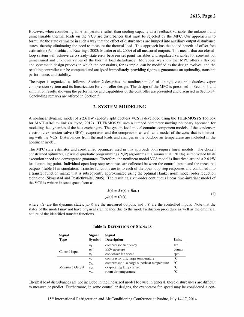
trol input and included in a straightforward manner. However, in the design that we consider, the evaporator fan iscontrolled by the occupant and its influence may instead be considered as a measured disturbance. Specifically, theevaporator fan speed will be fixed at a constant value in this design.
Compressor
Electronic Expansion
valve
evap fan speed
EEV position
cond fan speed
comp freq
A. B.
zone
Controller
VCS and Zone
outdoor air temp
thermal load
r(k) ym(k)u(k)
d(k)
Figure 1: (A) VCS schematic and (B) Block diagram of controller interacting with the VCS and Zone.
3. CONTROLLER DESIGN
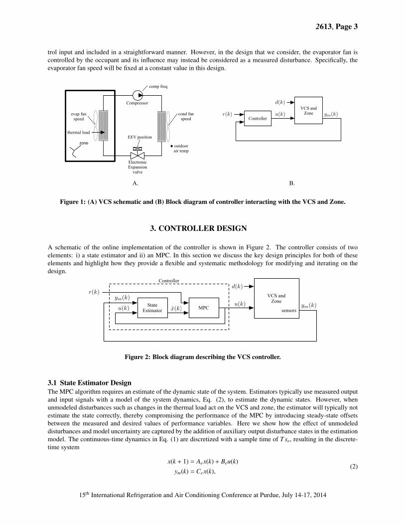
A schematic of the online implementation of the controller is shown in Figure 2. The controller consists of twoelements: i) a state estimator and ii) an MPC. In this section we discuss the key design principles for both of theseelements and highlight how they provide a flexible and systematic methodology for modifying and iterating on thedesign.
MPC
VCS and Zone
sensors
Controller
ym(k)
r(k)
u(k)
d(k)
State Estimator x(k)
ym(k)
u(k)
Figure 2: Block diagram describing the VCS controller.
3.1 State Estimator DesignThe MPC algorithm requires an estimate of the dynamic state of the system. Estimators typically use measured outputand input signals with a model of the system dynamics, Eq. (2), to estimate the dynamic states. However, whenunmodeled disturbances such as changes in the thermal load act on the VCS and zone, the estimator will typically notestimate the state correctly, thereby compromising the performance of the MPC by introducing steady-state offsetsbetween the measured and desired values of performance variables. Here we show how the effect of unmodeleddisturbances and model uncertainty are captured by the addition of auxiliary output disturbance states in the estimationmodel. The continuous-time dynamics in Eq. (1) are discretized with a sample time of T se, resulting in the discrete-time system
x(k + 1) = Aex(k) + Beu(k)ym(k) = Cex(k),
(2)
15th International Refrigeration and Air Conditioning Conference at Purdue, July 14-17, 2014

2613, Page 4
where k is the sampling index. The set of measured outputs ym is divided into two (potentially overlapping) subsets:performance outputs and constrained outputs. The MPC relies on a prediction model to determine the optimal controlinputs that achieve offset-free tracking of the performance outputs and to guarantee that the constrained outputs staywithin their bounds in the presence of unmodeled disturbances or modeling error. This can be achieved by augmentingthe estimator model with auxiliary states w 2 Rp⇥1, where p is the number of measured outputs in the system (Pan-nocchia and Rawlings, 2003; Maeder et al., 2009). Each of the auxiliary states is defined as the difference between anoutput as predicted by Eq. (2) and the actual measured value of the output.
The augmented estimator model takes the form
x(k + 1) = Aex(k) + Beu(k) (3a)w(k + 1) = Iw(k) (3b)
ym(k) = Cex(k) + Iw(k), (3c)
where I is the p ⇥ p identity matrix. Finally, the estimator dynamics are given by"x(k + 1)w(k + 1)
#=
"Ae � Le1Ce �Le1�Le2Ce I � Le2
# "x(k)w(k)
#+
"Be0
#u(k) +
"Le1Le2
#ym(k), (4)
where Le =hL0e1 L0e2
i0is the static estimator gain which can be designed using standard Kalman filtering techniques
(Simon, 2006).
3.2 MPC DesignThe MPC relies on the design of a prediction model and a cost function to be minimized.
3.2.1 Prediction Model For MPC, a discrete-time model of the system dynamics is used to predict the system responseover the chosen prediction horizon.
x(k + 1) = Apr x(k) + Bpru(k) (5a)yc(k) = Cpr x(k) (5b)yp(k) = Epr x(k) (5c)
Equation (5) provides a state-space realization of the prediction model and is based on a discretization of the system ofEq. (1) with a sample time of T spr such that T spr � T se. To emphasize that the discretization of the prediction modelis not necessarily the same as that of the estimator model, the subscript pr is appended to the state, input, and outputmatrices. The output matrix Cpr contains those rows of C such that yc, Eq. (5b), describes the outputs to be constrainedby the MPC. Similarly, Epr contains those rows of C such that yp, Eq. (5c), describes the performance outputs thatare explicitly characterized in the MPC cost function (Section 3.2.2). The structure of the prediction model allows forconstrained variables and performance variables to be added or removed from the controller design, highlighting theflexibility of the MPC design process.
Multiple augmentations need to be made to Eq. (5) so that the resulting MPC problem can be solved as a constrainedquadratic program (QP). First, the prediction model is augmented with the same auxiliary output disturbance statesthat were added to the estimator model so that the prediction model predicts the effect of control decisions on theconstrained and performance outputs,
"x(k + 1)w(k + 1)
#=
"Apr 00 I
# "x(k)w(k)
#+
"Bpr0
#u(k) (6a)
yc(k) =hCpr Cw
i " x(k)w(k)
#(6b)
yp(k) =hEpr Ew
i " x(k)w(k)
#, (6c)
where Cw and Ew are matrices of zeros and ones such that Eqs. (6b) and Eq. (6c) are consistent with Eq. (3c).
15th International Refrigeration and Air Conditioning Conference at Purdue, July 14-17, 2014
2613, Page 5
The second modification involves expressing the input as a discrete integrator (Di Cairano et al., 2013b). This changeof variables enables constraints to be placed on the rate of change of the control input and ensures that the cost functionhas a minimum at zero. Furthermore, we append the constrained output vector, yc, with yu = xu as shown in Eq. (7c)in order to enforce constraints on the actual values of the control inputs. Let u(k) = u(k � 1) + du(k), xu(k) = u(k � 1),and u = du(t), giving
2666666664
x(k + 1)w(k + 1)xu(k + 1)
3777777775 =
2666666664
Apr 0 Bpr0 I 00 0 I
3777777775
2666666664
x(k)w(k)xu(k)
3777777775 +
2666666664
Bpr0I
3777777775 u(k) (7a)
"yc(k)yu(k)
#=
"Cpr Cw 00 0 I
# 2666666664
x(k)w(k)xu(k)
3777777775 (7b)
yp(k) =hEpr Ew 0
i2666666664
x(k)w(k)xu(k)
3777777775 . (7c)
Finally, the state vector is augmented with the reference signal(s), i.e., the setpoints for the performance outputs: roomair temperature and compressor discharge temperature. By augmenting the prediction model in this manner, the costfunction (Section 3.2.2) can be designed to minimize z = yp � r, the error between the measured and desired valuesof the performance outputs as shown in Eq. (8c). The room air temperature reference r1 is an exogenous signal and isassumed to be constant over the prediction horizon, i.e. r1(k + 1) = r1(k). The compressor discharge temperature isdefined as a linear function of the compressor frequency: r2(k + 1) = r2(k) + c · u2(k). Let xr = r, giving
26666666666664
x(k + 1)w(k + 1)xu(k + 1)xr(k + 1)
37777777777775=
26666666666664
Apr 0 Bpr 00 I 0 00 0 I 00 0 0 I
37777777777775
26666666666664
x(k)w(k)xu(k)xr(k)
37777777777775+
26666666666664
Bpr0I
Br
37777777777775
u(k) (8a)
"yc(k)yu(k)
#=
"Cpr Cw 0 00 0 I 0
#26666666666664
x(k)w(k)xu(k)xr(k)
37777777777775
(8b)
z(k) =hEpr Ew 0 �I
i26666666666664
x(k)w(k)xu(k)xr(k)
37777777777775, (8c)
where Br =h
c 0 00 0 0
i.
3.2.2 Cost Function For any type of optimal controller, one needs to mathematically describe the quantity to beminimized or maximized. For linear MPC, it is common to design a quadratic cost function,
J = x(N)0Px(N) +N�1X
k=0
z(k|t)0Qzz(k|t) + u(k|t)0Ru(k|t), (9)
where x(k) =hx(k)0 w(k)0 xu(k)0 xr(k)0
i0, z = yp � r, u = u(k) � u(k � 1), and the term x(N)0Px(N) is the terminal
cost that is included to guarantee local asymptotic stability of the model predictive controller. See the Appendix fora sketch of the proof of stability and the determination of the terminal cost weight P. The matrices Qz and R aretunable weights that influence the transient performance of the controller by penalizing the individual terms of the costfunction. Finally, the cost function is minimized such that constraints
ymin y(k|t) ymax, k = 0, . . . ,Nc (10a)umin u(k|t) umax, k = 1, . . . ,Nu (10b)
15th International Refrigeration and Air Conditioning Conference at Purdue, July 14-17, 2014
2613, Page 6
0 500 1000 1500 200016182022242628
Room
Tem
pera
ture
( C)
Measured SignalSetpoint
0 500 1000 1500 200070
75
80
85
Com
pres
sor D
ischa
rge
Tem
pera
ture
( C)
Time (s)
(a) t = 0 until t = 2000 seconds.
2000 2500 3000 3500 4000 4500 500016182022242628
Room
Tem
pera
ture
( C)
Measured SignalSetpoint
2000 2500 3000 3500 4000 4500 500070
75
80
85
Com
pres
sor D
ischa
rge
Tem
pera
ture
( C)
Time (s)
(b) t = 2000 until t = 5000 seconds.
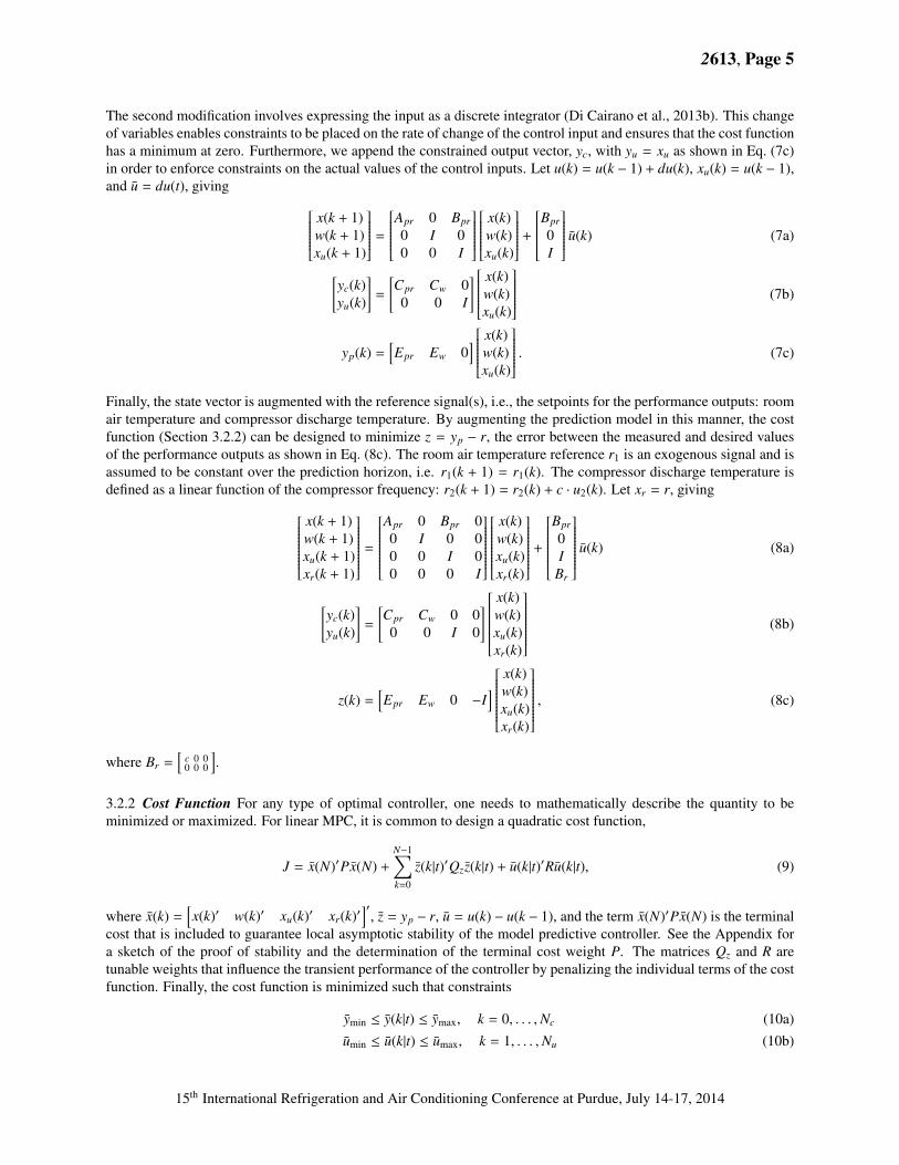
Figure 3: Regulation of performance variables.
are satisfied, where Nc and Nu are the time horizons over which the output and input constraints are enforced in theMPC. The prediction model, cost function, and constraints are converted into a quadratic program as described in DiCairano and Bemporad (2010).
4. SIMULATED CASE STUDY
In order to demonstrate the advantages of MPC for VCSs, a linear MPC was designed according to the procedureoutlined in the previous section and then tested on the nonlinear 2.6kW split-ductless VCS model. The outdoor airtemperature is held constant at 34�C throughout the simulation. The sample time of the estimator, T se, is 1 second,and the control inputs are updated at T spr = 15 seconds. Finally, the prediction horizon has a length of 64 steps, or 16minutes. The 5000 second simulation highlights the ability of the MPC to reject unknown thermal loads and operatethe system within specified input and output constraints while still optimizing performance tracking objectives.
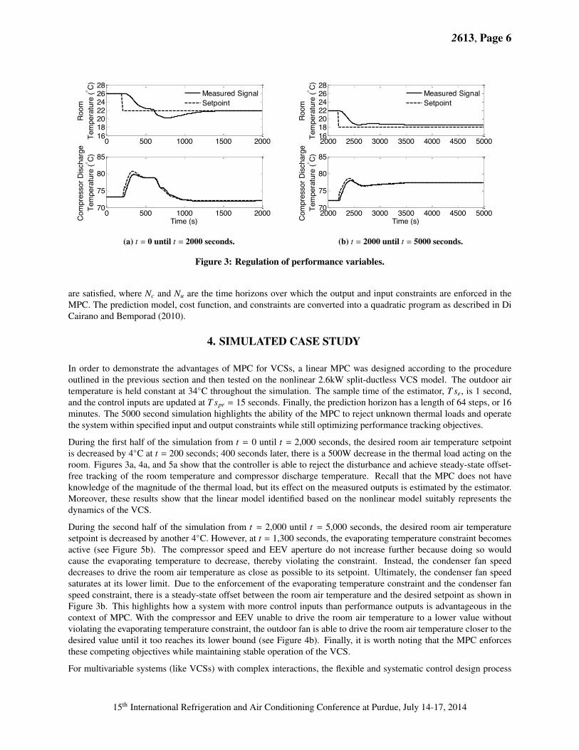
During the first half of the simulation from t = 0 until t = 2,000 seconds, the desired room air temperature setpointis decreased by 4�C at t = 200 seconds; 400 seconds later, there is a 500W decrease in the thermal load acting on theroom. Figures 3a, 4a, and 5a show that the controller is able to reject the disturbance and achieve steady-state offset-free tracking of the room temperature and compressor discharge temperature. Recall that the MPC does not haveknowledge of the magnitude of the thermal load, but its effect on the measured outputs is estimated by the estimator.Moreover, these results show that the linear model identified based on the nonlinear model suitably represents thedynamics of the VCS.
During the second half of the simulation from t = 2,000 until t = 5,000 seconds, the desired room air temperaturesetpoint is decreased by another 4�C. However, at t = 1,300 seconds, the evaporating temperature constraint becomesactive (see Figure 5b). The compressor speed and EEV aperture do not increase further because doing so wouldcause the evaporating temperature to decrease, thereby violating the constraint. Instead, the condenser fan speeddecreases to drive the room air temperature as close as possible to its setpoint. Ultimately, the condenser fan speedsaturates at its lower limit. Due to the enforcement of the evaporating temperature constraint and the condenser fanspeed constraint, there is a steady-state offset between the room air temperature and the desired setpoint as shown inFigure 3b. This highlights how a system with more control inputs than performance outputs is advantageous in thecontext of MPC. With the compressor and EEV unable to drive the room air temperature to a lower value withoutviolating the evaporating temperature constraint, the outdoor fan is able to drive the room air temperature closer to thedesired value until it too reaches its lower bound (see Figure 4b). Finally, it is worth noting that the MPC enforcesthese competing objectives while maintaining stable operation of the VCS.
For multivariable systems (like VCSs) with complex interactions, the flexible and systematic control design process
15th International Refrigeration and Air Conditioning Conference at Purdue, July 14-17, 2014
2613, Page 7
0 500 1000 1500 20000
50
100Co
mp.
Freq
. (Hz
)
0 500 1000 1500 20000
200
400
EEV
Aper
ture
(Cou
nts)
0 500 1000 1500 2000500
1000
Cond
. Fan
Sp
eed
(rpm
)
Time (s)
(a) t = 0 until t = 2000 seconds.
2000 2500 3000 3500 4000 4500 50000
50
100
Com
p.
Freq
. (Hz
)
2000 2500 3000 3500 4000 4500 50000
200
400
EEV
Aper
ture
(Cou
nts)
2000 2500 3000 3500 4000 4500 5000500
1000
Cond
. Fan
Sp
eed
(rpm
)
Time (s)
(b) t = 2000 until t = 5000 seconds.
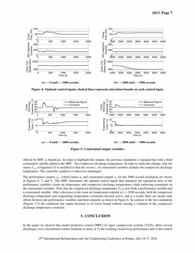
Figure 4: Optimal control inputs; dashed lines represent saturation bounds on each control input.
0 500 1000 1500 20001020304050
Com
p.
Disc
harg
eSu
perh
eat (
C)
0 500 1000 1500 20000
5
10
Evap
orat
ing
Tem
p. ( C)
Time (s)
Measured SignalConstraint
(a) t = 0 until t = 2000 seconds.
2000 2500 3000 3500 4000 4500 50001020304050
Com
p.
Disc
harg
eSu
perh
eat (
C)
2000 2500 3000 3500 4000 4500 50000
5
10
Evap
orat
ing
Tem
p. ( C)
Time (s)
Measured SignalConstraint
(b) t = 2000 until t = 5000 seconds.
Figure 5: Constrained output variables.
offered by MPC is beneficial. In order to highlight this feature, the previous simulation is repeated but with a thirdconstrained variable added to the MPC - the compressor discharge temperature. In order to make this change, only thematrix Cpr in Equation (5) is modified so that the vector yc of constrained variables includes the compressor dischargetemperature. The controller synthesis is otherwise unchanged.
The performance outputs yp, control inputs u, and constrained outputs yc for the 5000 second simulation are shownin Figures 6, 7, and 8. The MPC determines the optimal control inputs that minimize the regulation error of theperformance variables (room air temperature and compressor discharge temperature) while enforcing constraints onthe constrained variables. Note that the compressor discharge temperature Td is now both a performance variable anda constrained variable. After a decrease in the room air temperature setpoint at t = 2200 seconds, both the compressordischarge temperature and evaporating temperature constraints become active, and as a result, there are steady-stateoffsets between the performance variables and their setpoints as shown in Figure 6. In contrast to the first simulation(Figures 3-5) the condenser fan cannot decrease to its lower bound without causing a violation of the compressordischarge temperature constraint.
5. CONCLUSION
In this paper we showed that model predictive control (MPC) of vapor compression systems (VCSs) offers severaladvantages over conventional control methods in terms of 1) the resulting closed-loop performance and 2) the control
15th International Refrigeration and Air Conditioning Conference at Purdue, July 14-17, 2014

2613, Page 8
0 1000 2000 3000 4000 500016182022242628
Room
Tem
pera
ture
( C)
Measured SignalSetpoint
0 1000 2000 3000 4000 500070
75
80
Com
pres
sor D
ischa
rge
Tem
pera
ture
( C)
Time (s)
Figure 6: Sim. 2 – Regulation of perfor-mance variables.
0 1000 2000 3000 4000 50000
50
100
Com
p.
Freq
. (Hz
)
0 1000 2000 3000 4000 50000
200
400
EEV
Aper
ture
(C
ount
s)
0 1000 2000 3000 4000 5000500
1000
Cond
. Fan
Sp
eed
(rpm
)
Time (s)
Figure 7: Sim. 2 – Optimal control inputs;dashed lines show saturation bounds.
0 1000 2000 3000 4000 500070
75
80
Com
p.
Disc
harg
eTe
mp.
( C)
0 1000 2000 3000 4000 50001020304050
Com
p.
Disc
harg
eSu
perh
eat (
C)
0 1000 2000 3000 4000 50000
10
20
Evap
orat
ing
Tem
p. ( C)
Time (s)
Measured SignalConstraint
Figure 8: Simulation 2 – Constrained outputs.
engineering design process. Rather than designing multiple individual loops to address the various constraints in thesystem, a single MPC was systematically designed for the VCS with multiple control inputs, performance objectives,and constraints. Moreover, the addition or subtraction of performance objectives or constraints requires only minorchanges to the state-space representation of the estimator and prediction models. Through a simulated case studyit was shown that with the state estimator augmented with auxiliary output disturbance states, unmeasured thermalload disturbances are rejected in the steady state by the controller to achieve offset-free tracking performance. TheMPC also maintains system operation within input and output constraints. Finally, the design presented here uses onlytemperature measurements typically available in production VCSs.
NOMENCLATUREk discrete time index x dynamic state Subscript p performance outputr reference (setpoint) y output c constrained output pr prediction modelT s sample time e estimator model r referenceu control input eq equilibrium u control inputw auxiliary state m measured output
15th International Refrigeration and Air Conditioning Conference at Purdue, July 14-17, 2014

2613, Page 9
REFERENCES
Alleyne, A. (2012). Thermosys 4 toolbox. University of Illinois at Urbana-Champaign.http://arg.mechse.illinois.edu/thermosys/.
Amano, K. (2012). Heat pump apparatus and control method thereof. EP Patent App. EP20,110,007,843.
Di Cairano, S. and Bemporad, A. (2010). Model predictive control tuning by controller matching. Automatic Control,IEEE Transactions on, 55(1):185–190.
Di Cairano, S., Brand, M., and Bortoff, S. A. (2013a). Projection-free parallel quadratic programming for linear modelpredictive control. International Journal of Control, 86(8):1367–1385.
Di Cairano, S., Pascucci, C. A., and Bemporad, A. (2012). The rendezvous dynamics under linear quadratic optimalcontrol. In Proceedings of the 51st IEEE Conference on Decision and Control, pages 6554–6559. IEEE.
Di Cairano, S., Tseng, H. E., Bernardini, D., and Bemporad, A. (2013b). Vehicle yaw stability control by coordinatedactive front steering and differential braking in the tire sideslip angles domain. Control Systems Technology, IEEETransactions on, 21(4):1236–1248.
Elliott, M. S. and Rasmussen, B. P. (2008). Model-based predictive control of a multi-evaporator vapor compressioncooling cycle. In Proceedings of the American Control Conference, pages 1463–1468.
Garcia, C. E., Prett, D. M., and Morari, M. (1989). Model predictive control: theory and practice—a survey. Automat-ica, 25(3):335–348.
Koeln, J. P. and Alleyne, A. G. (2013). Decentralized controller analysis and design for multi-evaporator vaporcompression systems. In Proceedings of the American Control Conference, pages 437–442.
Maeder, U., Borrelli, F., and Morari, M. (2009). Linear offset-free model predictive control. Automatica, 45(10):2214–2222.
Pannocchia, G. and Rawlings, J. B. (2003). Disturbance models for offset-free model-predictive control. AIChEJournal, 49(2):426–437.
Simon, D. (2006). Optimal state estimation: Kalman, H infinity, and nonlinear approaches. John Wiley & Sons.
Skogestad, S. and Postlethwaite, I. (2005). Multivariable Feedback Control: Analysis and Design. John Wiley andSons Ltd.
Wallace, M., Das, B., Mhaskar, P., House, J., and Salsbury, T. (2012). Offset-free model predictive control of a vaporcompression cycle. Journal of Process Control, 22(7):1374–1386.
APPENDIX
Here we provide the reader with a proof guaranteeing local asymptotic stability of the MPC described in Section 3.We will make use of the prediction model, Eq. (8), rewritten in the following form,
"⇠(k + 1)r(k + 1)
#=
"A⇠ 00 Ar
# "⇠(k)r(k)
#+
"B⇠0
#u(k) (11a)
y(k) =hC⇠ 0
i "⇠(k)r(k)
#+ D⇠u(k) (11b)
z(k) =hE⇠ �Er
i "⇠(k)r(k)
#, (11c)
where ⇠(k) =hx(k)0 w(k)0 xu(k)0
i0, r(k) = xr(k), and z(k) = z(k).
15th International Refrigeration and Air Conditioning Conference at Purdue, July 14-17, 2014

2613, Page 10
Consider the MPC finite horizon optimal control problem
minU(t)
����h⇠(N)r(N)
i����2
P+
N�1X
k=0
kz(k|t)k2Qz+ ku(k|t)k2R (12a)
s.t. ymin y(k|t) ymax, k = 0, . . . ,Nc (12b)umin u(k|t) umax, k = 1, . . . ,Nu (12c)u(k|t) = K
h⇠(k|t)r(k|t)i, k = Nu, . . . ,N � 1 (12d)
where the objective is to design the terminal cost weight P and the terminal gain K such that the tracking error islocally asymptotically stable. In order to do this we apply with some modifications the results in Di Cairano et al.(2012). In details from (11a) and (11c), we construct the system
x(k + 1) = Apr x(k) + Bpru(k) (13a)z(k) = Epr x(k), (13b)
where x =⇥ ⇠
r⇤, Apr =
h A⇠ 00 Ar
i, Bpr =
hB⇠0
i, and Epr = [ E⇠ �Er ]. Note that (13) is not fully observable and not fully
controllable because the controller cannot, in general, modify the reference, and the optimal cost does not depend onthe absolute reference and output values but only on their difference. Therefore, a standard terminal cost design basedon LQR fails for this system. We apply an observability decomposition via an appropriate change of coordinates Tsuch that xobs = T x, xobs =
hx0o x0no
i0, and
xobs(k + 1) ="
Ao 0Ano,o Ano
# "xo(k)xno(k)
#+
"BoBno
#u(k) (14a)
z(k) =hEo 0
i " xo(k)xno(k)
#, (14b)
where xno are the coordinates of the state vector with respect to a basis of the unobservable space, and the pair (Ao, Eo)is observable.
Theorem 1 Let K = [ Ko 0 ] T and P = T 0h
Po 00 0
iT where
Ko = �(B0oPoBo + R)�1B0oPoAo (15)
and Po is the solution of the Riccati equation
Po = E0oQzEo + A0oPoAo � A0oPoBo(B0oPoBo + Ro)�1B0oPoAo (16)
which is assumed to exist. Then, the MPC controller that solves Eq. (12) ensures that limt kz(t)k = 0, and the trackingerror z(t) is locally asymptotically stable. Furthermore, if A⇠, Ar do not share unstable eigenvalues such that theeigenvectors images through E⇠, and Er share a subspace, there exists ⇠eq 2 Rdim(A⇠) with k⇠eqk < 1 such thatlimt k⇠(t) � ⇠eqk = 0.
Proof 1 (Sketch) The tracking problem, Eq. (12), is equivalent to a rendezvous problem of a controlled system, theplant, and an uncontrollable system, the reference. In Di Cairano et al. (2012) it was shown that the solution of the LQproblem for the observable subsystem, Eqs. (15),(16), is optimal for the rendezvous problem which is non-observable.Thus, K, P are optimal for the observable system LQ problem and asymptotically stabilize the observable componentof the system state, and hence the tracking error, which is related to such observable component by Eq. (14b). Whenthe MPC cost function, Eq. (12a), and terminal control law, Eq. (12d), are defined by K, P, the MPC behaves as theLQ-optimal controller, for all x 2 O1(Apr+ BprK), which is the maximum output admissible set of (Apr+ BprK), subjectto its constraints,Eqs. (12c),(12b). Thus, the first claim is proved. The second claim is proved by exploiting the resultsof Di Cairano et al. (2012). The zero dynamics (i.e., the dynamics when the output, which here is the tracking error, isconstantly zero) is equal to the residual dynamics after rendezvous, which is determined by the common eigenvalueswith associated eigenvectors having common image through the respective output matrices, E⇠, Er. If there are notsuch unstable eigenvalues, then the state of the system is bounded. ⇤
15th International Refrigeration and Air Conditioning Conference at Purdue, July 14-17, 2014