Embed Size (px)
Citation preview

UNIVERSIDAD DE CHILE FACULTAD DE CIENCIAS FÍSICAS Y MATEMÁTICAS DEPARTAMENTO DE INGENIERÍA DE MINAS
“MODEL PREDICTIVE CONTROL OF FROTH FLOTATION PROCESSES AIDED BY A
DYNAMIC SIMULATOR”
TESIS PARA OPTAR AL GRADO DE MAGISTER EN CIENCIAS DE LA INGENIERIA MENCION METALURGIA EXTRACTIVA
OCTAVIO FRANCISCO FUENZALIDA GONZALEZ
PROFESOR GUIA: WILLY KRACHT GAJARDO
PROFESOR CO-GUIA: LEANDRO VOISIN ARAVENA
MIEMBROS DE LA COMISION:
CLAUDIO ACUÑA PEREZ CHRISTIAN IHLE BASCUÑAN
SANTIAGO DE CHILE 2018

i
ABSTRACT
A model and simulation based methodology is used to implement a multi-layer
model predictive control (MPC) strategy for a rougher row of mechanical flotation cells.
Pilot-scale tests are done to calibrate and validate both the process simulation models
and the predictive simulation models. The hierarchical control strategy considers three
layers: orchestrator, advanced control and basic control; is deployed, in a commercial
control system and, tested in a pilot row.
The orchestrator is divided in two: the row supervisor and the row optimizer. The
row supervisor monitors and manages all the other components of the control
structure. The optimizer is a MPC-based controller which optimal criterion is
separation efficiency (SE) and; according to recent developments, that happens with a
balanced mass-pull profile along the row. The advanced control layer includes
individual cell MPC in coordination with a symbolic MPC for all pulp levels along the
row. The basic control layer consists of single loop proportional and integral (PI)
controllers and their corresponding valves and instruments. After simulation, the
control layers are successively downloaded in an industrial controller, starting from the
basic control layer and ending with orchestrator’s algorithms. Then, the control
structure provides good disturbance rejection against feed variabilities. Regarding the
orchestrator, it supports smooth and logical transitions between control modes as well
as good abnormal situation management.
This work shows promising results of the power of integrated process control
design and model based methodologies; allowing earlier and better selection and
validation of: flotation machine technology, cutting edge instrumentation and,
advanced control structure and strategies. Given pre-defined economic assumptions,
estimated results are obtained for the simulated industrial scenario: almost 40 percent
reduction of capital expenditure (Capex), with almost the same operational expenditure
(Opex). From the total Capex reduction, almost 80% is due to integrated process and
control design (IPCD), being the other 20% a consequence of advanced process control
and optimization structure and strategies. MPC-based control algorithms show their
potential to have a main role in mineral processing processes’ feasibility and optimality.
Keywords: control strategy, flotation, MPC, simulations.

ii
RESUMEN
Se utiliza una metodología basada en modelos y simulaciones para implementar
una estrategia de control predictivo basado en modelos (MPC) de varias capas para una
fila de celdas de flotación mecánica Rougher. Las pruebas a escala piloto se realizan
para calibrar y validar los modelos de simulación tanto de procesos como de
predicciones. La estrategia de control jerárquico considera tres capas: orquestador,
control avanzado y control básico; se implementa, en un sistema de control comercial y
se prueba en una fila de piloto.
El orquestador se divide en supervisor y optimizador de fila. El supervisor de fila
supervisa y administra todos los demás componentes de la estructura de control. El
optimizador está basado en MPC y su criterio óptimo es la eficiencia de separación (SE)
con un perfil de recuperación en peso equilibrado a lo largo de la fila. La capa de control
avanzado incluye un MPC de celda individual en coordinación con un MPC simbólico
para todos los niveles de pulpa a lo largo de la fila. La capa de control básica consiste en
controladores proporcionales e integrales (PI) y sus válvulas e instrumentos
correspondientes. Después de la simulación, las capas de control se descargan
sucesivamente en un controlador industrial, desde la capa de control básica hasta el
orquestador. La estructura de control logra un buen rechazo de perturbaciones de
alimentación. En cuanto al orquestador, admite transiciones suaves y lógicas entre los
modos de control, así como una buena gestión de situación anormal.
Este trabajo muestra resultados prometedores del poder del diseño de control de
procesos integrado y de las metodologías basadas en modelos; permitiendo una mejor y
más temprana selección y validación de: tecnología de máquina de flotación,
instrumentación y estructura de control avanzada. Dados los supuestos económicos
predefinidos, se obtienen resultados estimados para el escenario industrial simulado:
casi 40 por ciento de reducción del gasto de capital (Capex), con casi el mismo gasto
operacional (Opex). De la reducción total de Capex, casi el 80% se debe al diseño
integrado de procesos y control (IPCD), siendo el otro 20% una consecuencia del
control avanzado del proceso y la estructura y estrategias de optimización. Los
algoritmos de control basados en MPC muestran su gran potencial.
Palabras clave: estrategia de control, flotación, MPC, simulaciones.

iii
DEDICATORY
To God
To Miriam, my ambassador in heaven
To Valeria, my first minister on earth

iv
ACKNOWLEDGEMENTS
I would like to express my gratitude to my advisor Professor Willy Kracht, for
giving me the opportunity of working with him. His wise words and insightful opinions
motivated me to bring out the best of me to accomplish this goal.

v
TABLE OF CONTENTS
ABSTRACT i
RESUMEN ii
DEDICATORY iii
ACKNOWLEDGEMENTS iv
LIST OF TABLES vii
LIST OF FIGURES viii
1. INTRODUCTION 1
1.1. CONTEXT AND WIDE PERSPECTIVE 1
1.2. RELEVANCE 1
1.3. THESIS OUTLINE 2
2. LITERATURE REVIEW 3
2.1. REVIEW METHODOLOGY AND SIMILAR WORKS 3
2.2. MODELING ESSENTIALS 8
2.3. STARTUP MODELS 11
2.3. PROCESS CONTROL 17
2.4. MODEL PREDICTIVE CONTROL 24
2.5. MPC STARTUP ALGORITHMS 28
3. OBJECTIVES AND SCOPE 32
3.1. OBJECTIVES 32
3.2. SCOPE 32
4. FLOTATION MACHINES SELECTION 33

vi
4.1. INDUSTRIAL CONTEXT 34
4.2. FLOTATION MACHINES 37
4.3. EXPLORATORY ROUGHER CAMPAIGN 40
4.4. ROUGHER VARIABILITY CAMPAIGN 45
5. PROCESS SIMULATION FRAMEWORK 52
5.1. SYSTEMS IDENTIFICATION STRATEGY 52
5.2. INSTRUMENTATION AND CONTROL 56
5.3. SINGLE CELL CHARACTERIZATION 59
5.4. ROW CHARACTERIZATION 70
6. ADVANCED CONTROL AND OPTIMIZATION 75
6.1. ADVANCED CONTROL PERSPECTIVE 75
6.2. ADVANCED CONTROL METHODOLOGY 76
6.3. CONTROL DESIGN 77
6.4. CONTROL SIMULATION FRAMEWORK 84
7. OVERALL DISCUSSION 88
7.1. MODELING 88
7.2. INSTRUMENTATION 89
7.3. ADVANCED CONTROL STRATEGY AND OPTIMIZATION 90
8. CONCLUSSIONS AND FINAL REMARKS 91
BIBLIOGRAPHY 93

vii
LIST OF TABLES
Table 4.1: Main FGUs and corresponding trench samples
Table 4.2: FGU’s proportions according to mining plan
Table 4.3: Main FGUs’ mineralogical characteristics
Table 4.4: Copper distribution in representative trench samples
Table 4.5: Summary of exploratory rougher tests
Table 4.6: Summary of variability campaign ore types
Table 4.7: Testing completed on phase 2 variability samples
Table 4.8: Group C Sample Characteristics
Table 5.1: Experimental sub phase I: Instrumentation and Control
Table 5.2: Experimental sub phase II: Single RS Cell Characterization
Table 5.3: Experimental sub phase III: Row Characterization
Table 5.4: Cells’ operational parameters
Table 5.5: RS three compartmental model fitting
Table 5.6: RS versus conventional three compartmental model fitting
Table 5.7: Conventional SALA cells’ RTD model fitting (time in seconds)
Table 5.8: RS-RTD model fitting
Table 5.9: Polat & Chandler (Rcp) and compartmental recoveries
Table 5.10: Total recoveries and errors related to experimental results
Table 6.1: Nominal values for row operational variables

viii
LIST OF FIGURES
Figure 2.1: Literature review using Venn approach
Figure 2.2: Typical grade versus recovery curve
Figure 2.3: Air recovery optimization, from Hadler & Cilliers, 2010
Figure 2.4: Generic flotation machine, from Yianatos, 2007a
Figure 2.5: Hydrodynamic zones in mechanical cells, from Gorain et al., 2000
Figure 2.6: Transfer of water and suspended particles, from Savassi, 2005
Figure 2.7: Transfer by true flotation mechanism, from Savassi, 2005
Figure 2.8: Mass transfer by true flotation and entrainment (Savassi, 2005)
Figure 2.9: Row of flotation cells, Kämpjärvi & Jämsä-Jounela (2003)
Figure 2.10: Optimization contextual scheme
Figure 2.11: Flotation control objective, from Wills (2006)
Figure 2.12: Basic MPC structure block diagram (from Bemporad et al., 2016)
Figure 2.13: Adaptive control scheme, adapted from Tao (2014)
Figure 4.1: Collective flotation circuit
Figure 4.2: Simulated copper and molybdenum grades
Figure 4.3: Simulated copper and molybdenum recoveries
Figure 4.4: Reactor Separator (RS) Machine
Figure 4.5: Mini-RS configuration schematic
Figure 4.6: Copper grade versus recovery with and without IWW
Figure 4.7: NSG versus copper recoveries with and without IWW
Figure 4.8: Effect of IWW - left with - right without
Figure 4.9: Effect of FWW for trucks 4 & 6
Figure 4.10: Impact of feed slurry density Truck 6
Figure 4.11: Copper Recovery – Denver versus RS
Figure 4.12: Denver Cu Recovery as a function of feed % Sulphides

ix
Figure 4.13: Delta Mass Recovery versus Delta Cu Rec'y
Figure 4.14: Delta Recovery versus feed -400 mesh fraction
Figure 5.1: System identification iterative work, from Ljung, 1990
Figure 5.2: Cell n; instrumentation and basic control scheme
Figure 5.3: Cell n, air flow control loop
Figure 5.4: Cell n, wash water flow control loop
Figure 5.5: Row instrumentation
Figure 5.6: Two compartment model (adapted from Savassi, 2005)
Figure 5.7: Full three compartmental model of conventional mechanical cell
Figure 5.8: Full three compartmental model of a RS flotation machine
Figure 5.9: Row measurements applied to one cell
Figure 5.10: SCRM + conventional cell three compartment model
Figure 5.11: Single cell row model + RS three compartment model
Figure 5.12: Experimental setup for conventional cell RTD
Figure 5.13: Experimental setup for RS machine RTD
Figure 5.14: Double cell row model
Figure 5.15: Triple cell row model
Figure 5.16: Four cell row model
Figure 6.1: Row control hierarchy
Figure 6.2: Cell-based advanced control scheme
Figure 6.3: Row-based advanced control scheme
Figure 6.4: Cell n froth stability observers
Figure 6.5: Balanced mass pull profile
Figure 6.6: Control structure block diagram
Figure 6.7: Control simulation framework

1
1. INTRODUCTION
This chapter is a concise presentation on the “why”, “what”, and “how” on the
subject. They are presented in the context, relevance and outline sections.
1.1. CONTEXT AND WIDE PERSPECTIVE
Minerals are valuable natural resources being finite and non-renewable. The
mining cluster is by no doubt the most important sector of Chilean economy. But,
mineral yields that have fed Chilean society for a long time are decreasing both in
quantity and quality. Further use of intelligence is needed in order to mitigate the
exhaustion of natural resources. Intelligence, whether natural or synthetic, derives from
a model of the world in which the system operates. Greater intelligence arises from
powerful and “fit for purpose” models, capable of strike a balance between accuracy and
interpretability of predictions. The software implementation of models is known as
simulator or simulation framework. A specific realization of a certain scenario in the
simulator is known as simulation. Model based design is well recognized as a systematic
approach to design and implement industrial plants.
1.2. RELEVANCE
Modern metallurgical plants shall be high efficient and that implies operation
near constraints with stronger attention to process dynamics and controls. In other
words, to optimize, processes shall be under control which needs good measurements.
Therefore, the role of process control systems has to be considered as an integrated
element of business planning in order to simultaneously ensure feasibility and
optimality of process operation. Model predictive control is a particular branch of
model-based design: a dynamical model of the open-loop process is explicitly used to
construct an optimization problem aimed at achieving prescribed system's performance
under specified restrictions on input/output variables.
2
Many attempts have been made to improve the flotation process itself. An
excellent review on the major developments up to the mid-1970 is compiled by Trahar
and Warren (1976). Some of them are still being used or revisited. Two main lines have
been followed; being the first one by reagents with the aim to enhance the
agglomeration of fine particles, increasing the probability of collision. The second line is
developing new cell machines with the aim to create more favorable hydrodynamic
conditions for flotation (i.e. Gorain et al., 2000). For nearly a century mechanical cells
have dominated the market. Faced with increasing demands to improve the processing
of fine particles, cell suppliers have shown their resilience by increased cell size; the use
of adjustable froth launders and; new agitation mechanisms (Yianatos, 2007a).
1.3. THESIS OUTLINE
Chapter 2 presents the literature review. As this work is related to more than one
field of knowledge, a Venn methodology is considered appropriate as starting point.
Then, references related to optimization, control design, modelling and MPC are shown.
In chapter 3, objectives and scope of this thesis are set. Chapter 4 is related to an
important part of the experimental work of this thesis; starting with the industrial
context with its given definitions and assumptions and followed by exploratory and
variability campaigns. Both campaigns are described and used to evaluate a non-
conventional flotation machine. In addition to its intrinsic value, the work in chapter 4
is used afterwards to implement, calibrate and validate an important fraction of both
process and prediction models; starting with the metallurgical modelling work at the
end of the chapter and; following by the process simulation framework described in
chapter 5. Chapter 6 explains the main specific application of this work: a hierarchical
model predictive control of a row of rougher flotation cells. Chapter 7 is the ending
chapter, where the discussion and conclusions of this thesis are presented.

3
2. LITERATURE REVIEW
2.1. REVIEW METHODOLOGY AND SIMILAR WORKS
Fit for purpose + self-explained: this review follows a fit for purpose approach and
then is focused on this thesis’ perspective. Nevertheless, appropriate context is given in
order to be self-explained.
Literature review methodology: this work is related to more than one field of
knowledge and therefore a Venn methodology is used and shown in figure 2.1. The
universe is the subject which in this case is rougher froth flotation using rows of
mechanical cells. Then, one set is the problem (optimization), the second set is
methodology (modelling) and the third set is the focus (control). Following Venn
methodology, the primary attention should be on similar works.
Figure 2.1: Literature review using Venn approach.
Optimization in mining, metal and mineral processing (Goodwin et al.,
2008): Every decision making problem involves some form of optimization, often
implicit rather than explicit. They state that making optimization explicit has many
advantages including the integration between technical and commercial information, as
a balanced approach to decision-making. Matching cost reporting areas to process areas
greatly assist management. A reasonably close match makes it much easier to estimate
the potential costs and benefits of process changes.
4
Goodwin et al. note that optimization can play a role at many levels in an
enterprise including: data reconciliation; single feedback loops; coordination of
feedback loops; interconnection of unit operations through the value chain(s); supply
chain management and; long-term corporate investment strategies. By the exception of
last two, all the other optimizations are under this thesis’ scope. The role of process
control has to be considered as an integrated element of business planning in order to
support feasibility and optimality of process operation. Process control systems shall
support asset management decision making through: dynamic optimization, abnormal
situation support systems and asset integrated information at central control room.
Dynamic optimization and abnormal situations are under the scope.
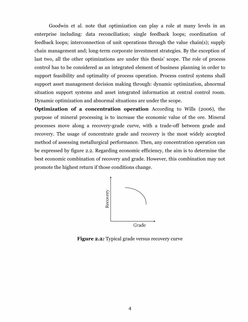
Optimization of a concentration operation According to Wills (2006), the
purpose of mineral processing is to increase the economic value of the ore. Mineral
processes move along a recovery-grade curve, with a trade-off between grade and
recovery. The usage of concentrate grade and recovery is the most widely accepted
method of assessing metallurgical performance. Then, any concentration operation can
be expressed by figure 2.2. Regarding economic efficiency, the aim is to determine the
best economic combination of recovery and grade. However, this combination may not
promote the highest return if those conditions change.
Figure 2.2: Typical grade versus recovery curve

5
Regarding technical efficiency, Schulze (1984) defines separation efficiency as
the difference between the recoveries of valuable and gangue minerals. According to
Wills (2006): “although the value of separation efficiency can be useful in comparing
the performance of different operating conditions on selectivity, it takes no account of
economic factors, and a high value of separation efficiency does not necessarily lead to
the most economic return”. Therefore, neither economics nor technical approaches can
define the optimum by themselves alone. This thesis considers separation efficiency
(SE) as optimal criterion, but the simulation framework has the flexibility to
incorporate and/or biases the optimal criterion based on economics.
Optimal control: Maldonado et al. (2007) study the optimal control of rougher
flotation rows. The row optimization objective is the minimization of the Cu tailing
grade given a desired final Cu concentrate grade. They conclude that their simulation
results show good correlations between their optimization strategy and actual operating
practices at the rougher flotation plant under study.
Profiling has been proposed as row dynamic optimizer (i.e. Seguel et al., 2015; Sing
and Finch, 2014 and; Hadler & Cilliers, 2010). Maldonado et al. (2011) find that, if
entrainment is neglected, the maximum SE is obtained when each of the cells along the
row has the same recovery. Singh and Finch (2014) confirm that with simulations and
industrial data and then, they use math and simulations to propose that, considering
entrainment, a balanced mass-pull profile is optimum. Seguel et al. (2015) revisit row
optimization through froth depth profiling and the following formulation of the
optimization problem: maximization of copper Cu recovery while satisfying a minimum
concentrate grade. Their conclusion is that optimal profile also provides a balanced
mass-pull profile. A balanced mass-pull profile is considered as base scenario herein,
but the simulation framework allows a balanced recovery profile.

6
In terms of control theory, profiling schemes are related to setpoint tracking.
Traditional model predictive controllers are tuning around a particular operating point,
fitting fairly well for fixed set-points but not necessarily for moving set-points.
Asymptotic tracking performance and stability is crucial for profiling based optimizing
applications and adaptive model predictive control (AMPC) family of algorithms is
capable to ensure system asymptotic tracking performance and stability under large
parametric, structural and parametric disturbance uncertainties (Tao, 2014). AMPC is
considered in this thesis for advanced profiling controllers.
Model predictive control applied to froth flotation: Rojas and Cipriano (2011)
use simulations to compare three control strategies, one conventional and two MPC-
based ones. Their assumption is that the optimum is achieved maximizing the recovery
and keeping the concentrate grade over a minimum. The first MPC strategy considers
row tailings and concentrates grades and the other MPC strategy includes estimation of
concentrate grade in intermediate cells. They conclude that even though both MPC
strategies deliver high performance regardless disturbances, the economic benefits
obtained with the second MPC strategy are greater, noting the importance of
intermediate measurements. Consequently, in this thesis: virtual sensors are developed
to estimate individual mass pulls and concentrate grades, including the intermediate
cells; the row instrumentation is used incrementally for further characterization and; in
other words, the instrumentation planned for the row is used for 1, 2, 3 and four cells.
Putz & Cipriano (2015) propose and simulate a hybrid model predictive control
(H-MPC) for rougher flotation. They define three operating modes for each rougher
flotation cell: no concentrate (sunken cell), normal operation and presence of pulp in
overflow of concentrate (pulping cell). Their approach emphasizes the relevance of MPC
algorithms, the modal nature of industrial froth flotation systems and the lack of
abnormal situation integration to control strategies. In this thesis, virtual sensors are
used for sunken and pulping cells.

7
Air recovery (Hadler & Cilliers, 2010): they add another component to mass pull
and recovery profiles, stating that air flowrate and froth depth could affect froth
structure and stability, which in turn could affect mass pull. They propose air recovery,
or the fraction of air entering a cell that overflows the lip, as measure of froth stability.
Air recovery, α, is determined using the over flowing froth velocity, Vf; the overflowing
froth height above the cell lip, h, the over flowing length, w, and the inlet air flowrate,
Qa, as shown in equation (2.1). A high air recovery, therefore, indicates a more stable
froth. The complement to the air recovery (1– 𝛼) gives the fraction of air that leaves
through bursting. They mention that “when operating a cell at the air rate that yields
the peak air recovery (PAR), an improvement in flotation performance, particularly
mineral recovery, can be obtained”. an increase in mass pull by means of a higher air
flow, increase mineral recovery as far as air rate peak is still not achieved.
α= Vf∙h∙w
Qa
(2.1)
Figure 2.3: Air recovery optimization, from Hadler & Cilliers, 2010
Brief of profiling methods: As a main conclusion, the technical optimum is
obtained by means of a balanced mass pull along the row. Then, a simple and practical
criterion for row optimization is given: balanced mass pull profile along the row. In this
thesis, air recovery is one of two froth stability indices. In addition, in almost all the
articles two variables are considered for profiling but only one at a time; in process
control words, setpoint tracking is needed for the “profiled variable” while setpoint
regulation is needed for the others.

8
2.2. MODELING ESSENTIALS
As this thesis is model-based, models are its pillars. In its essence, process
modelling is an exercise of translation of knowledge about the process into an abstract
mathematical representation (Cameron & Hangos, 2001). The nature of knowledge is
diverse and thus modelling methods can naturally be segmented accordingly: white box
models represent a broad class of models based on physical or chemical laws; black box
models represent a modelling framework based exclusively on process data and; grey
box parametric models where the model structure is first-principle-based, but the
model fitting is data driven. Here, both process and control simulation sub systems are
built upon a selection and synthesis of white, black and grey box models.
As part of the modelling’s synthesis work of this thesis; the following golden rules
are almost everywhere a good modelling work has been done:
Golden Rule 1: Simple. According to Brooks (1991), there is little point in creating a
model if it has all the complexity of the object it is modelled after. The best model of
every system is itself. The single key component of a model is simplification.
Golden Rule 2: Incremental. According to Luyben (1990), the first design should be
based on simple models with low number of estimated parameters and globally
convergent and then further details should be incorporated as available and needed.
Golden Rule 3: Modular. A set of comprehensive models is better than single mega
models. According to Brooks (1991), general purpose models that try to in incorporate
practically everything shall be avoided. Such models are difficult to validate, to
interpret, to calibrate statistically and, most importantly, to explain.
Golden Rule 4: Fit for purpose. Matzopoulos (2011) states that unneeded details
increase calculation times and reduce model robustness. He also recommends to
implement fit-for-purpose models that could be “parameterized” in order to easily
include or exclude phenomena. In other words, the model has to be useful or otherwise
there would be little point in creating the model.

9
Flotation modeling (Yianatos, 2007a): flotation is a solid–solid separation, where
fine solid particles, suspended in water contact an air bubble in well-mixed air–pulp
dispersion. Flotation separation is based on different mineral surface properties:
hydrophobic particles can attach to air bubbles, while hydrophilic particles do not. Then,
hydrophobic particles can be selectively separated by levitation against gravity in the
aqueous medium. A generic flotation machine can be observed as a sequence of two
operations, ‘reaction’ and ‘separation’, as shown in figure 2.4. The reactor is fed with: the
pulp containing the solids to be separated; chemical reagents to produce selective
aggregation of particles with air bubbles and; energy to keep the solids in suspension
and to disperse the air into fine bubbles”.
Figure 2.4: Generic flotation machine (from Yianatos, 2007a)
The collection process has been represented similar to a chemical reaction; being
the ‘reactants’ hydrophobic mineral particles that collide with and adhere to air bubbles.
The reaction ‘product’ is a particle-bubble aggregate that is less dense than the medium
and moves upwards against gravity while hydrophilic particles are reported down to the
tails. A necessary condition for mineral separation in a flotation process is the existence
of a froth zone with a distinctive pulp-froth interface. The critical boundary conditions
for industrial flotation equipment in terms of bubble size and superficial gas rate,
regarding the loss of the pulp–froth interface, froth stability and limiting carrying
capacity has been reported by Yianatos and Henrıquez (2007b).

10
Compartmental models: the compartmental approach to model flotation involves
the division of the flotation cell contents into two or more zones that combine to form a
coherent system. The subprocesses occurring in each phase are collectively represented
by an equivalent macroprocess.
For mechanical cells, Arbiter and Harris ( 1962) are among the first to take the
froth phase into account. Their two-phase model of the flotation process is based on the
assumption that both pulp and froth are well-mixed. Harris et al. (1963) and Harris &
Rimmer (1966), carry out extensive testing of the two-phase model under steady state
and transient conditions. As a theoretical improvement of the well-mixed hypothesis
some authors describe froth behavior by applying plug-flow models as Cutting &
Divinish (1975).
The first three compartment model for mechanical cells is proposed by
Hanumanth and Williams (1992); including drainage of solids in the froth layer, and its
dependence on froth height. They also outline procedures to estimate the parameters of
the model, and validate the model comparing its predictions with experimental results.
Gorain & Franzidis & Manlapig (2000), describe mechanical cells as having three
distinctive hydrodynamic zones. According to them, a mechanical flotation cell needs
three hydrodynamic zones for effective flotation. They define the collection zone as the
region close to the impeller that gives the turbulence needed for: solids suspension; gas
dispersion and; bubble-particle interaction for minerals’ collection. According to them,
the quiescent zone is a relatively less turbulent region above the collection zone where
the bubble-particle aggregates rise up. They note that the quiescent zone reduce the
number of gangue minerals which may have been entrained mechanically or entrapped
between bubbles for upgrading of valuable minerals. They remark that the froth zone
above the quiescent zone serves as an additional cleaning step and improves the grade
of the concentrate product. The three hydrodynamic zones in mechanical flotation cells
are shown in next figure 2.5.

11
Figure 2.5: Hydrodynamic zones in mechanical cells (from Gorain et al., 2000)
2.3. STARTUP MODELS
Three models are considered herein as starting points in terms of froth flotation
modeling synthesis: Savassi’s (2005) compartmental model; Kämpjärvi & Jämsä-
Jounela (2003) dynamic model and; Polat & Chandler (2000) collection zone model. In
this sub-chapter, these three models are described using – almost - authors’ own words.
Savassi´s model description (from Savassi, 2005): figure 2.6 shows Savassi’s
model for water (left) and suspended particles (right) in terms of the following
flowrates: F, feed throughput; Y, suspension due to impeller action; I, influx to the
froth; D, drainage from the froth; X, re-circulation by both impeller action and particle
settling; C, concentrate; T, tail. The subscript “s” when applied to the pulp indicates
suspended particles, but the same subscript when applied to the froth indicates
particles that crossed the pulp–froth interface by entrainment (whether or not those
particles remain suspended in water all the way to the concentrate launder).
The transfer of a target particle class by true flotation mechanism is illustrated in
Fig. 2.7. The flowrate D represents the drop-back of attached particles from the froth
due to detachment followed by drainage. Note that the subscript A when applied to the
pulp indicates particles attached to air bubbles, but the same subscript when applied to
the froth indicates particles originally attached to bubbles before entering the froth”.

12
Figure 2.6: Transfer of water and suspended particles, from Savassi (2005)
Figure 2.7: Transfer by true flotation mechanism, from Savassi (2005)
Then, for a particular valuable particle class, the total recovery by means of true
flotation is given by:
Rtot=Rc∙Rf
1-Rc∙(1-Rf) (2.2)
Next figure 2.8 shows the mass transfer by true flotation and entrainment. Any
particle suspended in the quiescent zone has three possible recent origins: rejection
from the froth due to water drainage, DS; rejection from the froth due to detachment
followed by water drainage, DA; and suspension from the bottom of the cell due to
impeller action, YS.
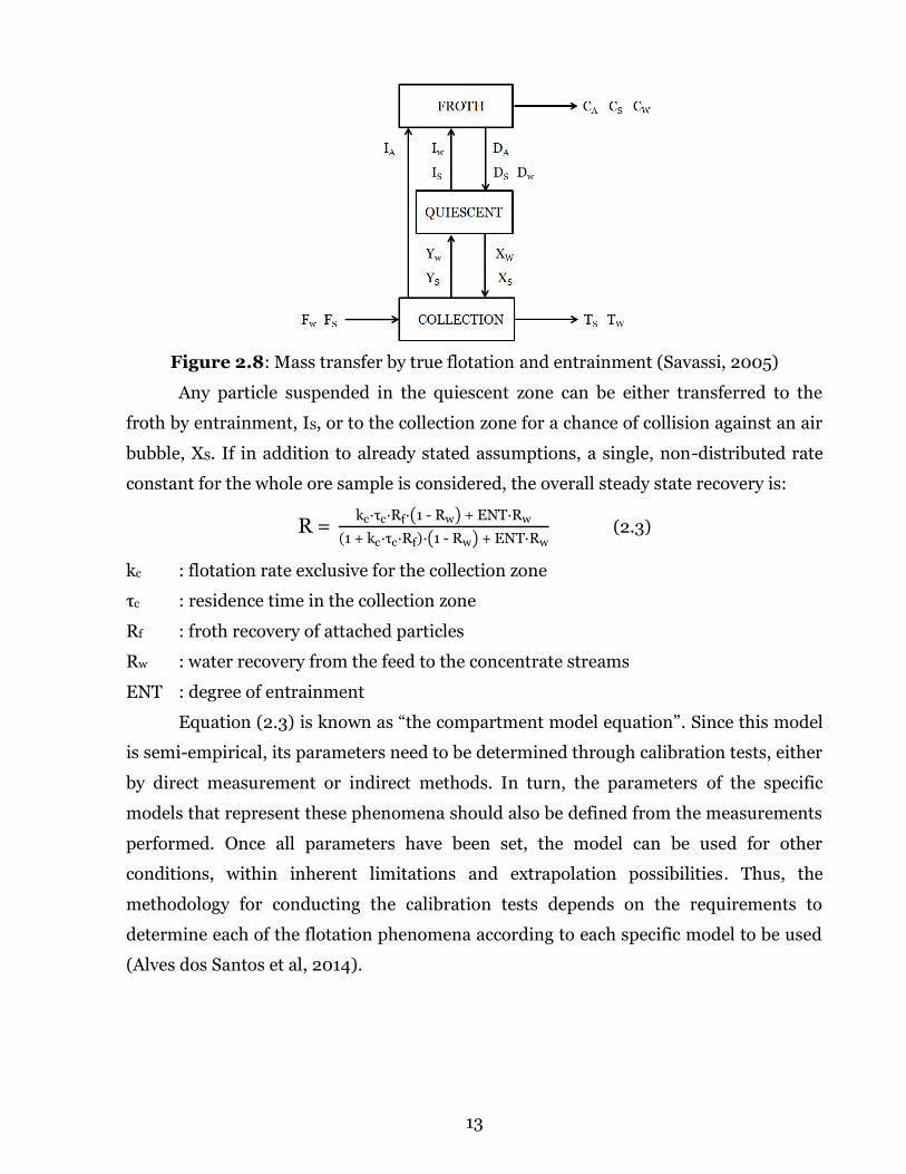
13
Figure 2.8: Mass transfer by true flotation and entrainment (Savassi, 2005)
Any particle suspended in the quiescent zone can be either transferred to the
froth by entrainment, IS, or to the collection zone for a chance of collision against an air
bubble, XS. If in addition to already stated assumptions, a single, non-distributed rate
constant for the whole ore sample is considered, the overall steady state recovery is:
R = kc∙τc∙Rf∙(1 - Rw) + ENT∙Rw
(1 + kc∙τc∙Rf)∙(1 - Rw) + ENT∙Rw (2.3)
kc : flotation rate exclusive for the collection zone
τc : residence time in the collection zone
Rf : froth recovery of attached particles
Rw : water recovery from the feed to the concentrate streams
ENT : degree of entrainment
Equation (2.3) is known as “the compartment model equation”. Since this model
is semi-empirical, its parameters need to be determined through calibration tests, either
by direct measurement or indirect methods. In turn, the parameters of the specific
models that represent these phenomena should also be defined from the measurements
performed. Once all parameters have been set, the model can be used for other
conditions, within inherent limitations and extrapolation possibilities. Thus, the
methodology for conducting the calibration tests depends on the requirements to
determine each of the flotation phenomena according to each specific model to be used
(Alves dos Santos et al, 2014).

14
Kämpjärvi & Jämsä-Jounela dynamic model: the simulation kernel for levels is a
symbolic implementation based on the model for pulp-level published by Kämpjärvi &
Jämsä-Jounela (2003) and represented by Figure 2.9 and equations (2.4) to (2.5) and
(2.6):
Figure 2.9: Diagram of flotation cells, Kämpjärvi & Jämsä-Jounela (2003)
Where y1, y2, y3 and, y4; are the pulp cell levels. u1, u2, u3 and, u4; are the
valves’ positions and; q is the volumetric feed to first cell. Then, for each cell along the
row, the corresponding volumetric balance is done:
dVi
dt= Q
F,i- QC,i - Q
T,i (2.4)
QFi, QCi and QTi are the corresponding volumetric flows at feed, concentrate and,
tailings. In addition, Vi is the pulp volume of cell i. Then, assuming that concentrate
volumetric flows could be neglected, for four cells:
dV1
dt= q- Q
T,1 (2.5)
dV2
dt= Q
T,1- QT,2 (2.6)
dV3
dt= QT,2- Q
T,3 (2.7)
dV4
dt= Q
T,3- Q
T,4 (2.8)
Then, a constant transversal area “S” is assumed, together with a constant
physical difference in height between the cells “a”. In addition the same valves are
assumed for all cell discharges and therefore, the valve coefficient “Cv“depends only on
the control variable “u”. Also, atmospheric discharge for cell 4 is assumed.

15
Using Bernoulli’s equation:
S∙dY1
dt=q- k∙CV(u1)∙√δ1∙g∙y
1-δ2∙g∙(y
2-a) (2.9)
S∙dY2
dt=k∙CV(u1)∙√δ1∙g∙y
1-δ2∙g∙(y
2-a)- k∙CV(u2)∙√δ2∙g∙y
2-δ3∙g∙(y
3-a) (2.10)
S∙dY3
dt=k∙CV(u2)∙√δ2∙g∙y
2-δ3∙g∙(y
3-a)- k∙CV(u3)∙√δ3∙g∙y
3-δ4∙g∙(y
4-a) (2.11)
S∙dY4
dt=k∙CV(u3)∙√δ3∙g∙y
3-δ4∙g∙(y
4-a)- k∙CV(u4)∙√δ4∙g∙y
4 (2.12)
Also, Jämsä-Jounela assumes constant densities along the row: δ1=δ2=δ3=δ4
and, extracts and group terms into K. Also, he doesn’t differentiate among real pulp
densities and apparent pulp densities (with gas holdup). Also, each level derivative
could be considered as space state component:
dY1
dt=(q S⁄ )- K∙CV(u1)∙√y
1-y
2+a =f1(Y,U) (2.13)
dY2
dt=k∙CV(u1)∙√y
1-y
2+a- k∙CV(u2)∙√y
2-y
3+a=f2(Y,U) (2.14)
dY3
dt=k∙CV(u2)∙√y
2-y
3+a- k∙CV(u3)∙√y
3-y
4+a=f3(Y,U) (2.15)
dY4
dt=k∙CV(u3)∙√y
3-y
4+a- k∙CV(u4)∙√y
4=f4(Y,U) (2.16)
Y and U are the vectors of pulp levels and, control actions; q is a measured
disturbance of low frequency and; Ẏ = F(Y, U) is the vector of derivatives. Then:
Ẏ = F(Y, U, Q) = [f1; f2; f3; f4] (2.17)
Linearizing around a symbolic operating point, (Yo, Uo) ⇒
Ẏ = F(Y, U, Q) ≅ F (Yo, Uo) + ∂F
∂Y(Yo, Uo)∙∆Y+
∂F
∂Y(Yo, Uo)∙∆U (2.18)
For pulp levels, the type of state space model being looked is the one expresses in
equation 2.19, it can be noticed that A and B are the discretized version of Jacobian of F
respect to Y and U, evaluated in the operating point (Yo, Uo). Qk is derived from the
volumetric flow q and IWW. Further details are found in the process simulation chapter
kQBuAyy kk1k (2.19)

16
Polat & Chandler (2000) collection zone recovery model: The general first
order recovery equation is:
R(t)=R∞∙[∬ (1-e-kt)∙F(k)∙E(t) dk dt∞
0] (2.20)
In which,
R(t) : Recovery at time t
R∞ : Maximum recovery (for t = ∞)
k : First order flotation rate constant, given in 1/s
(1-e-kt) : Recovery of floatable mineral according to a first order process
F (k) : Kinetic distributions function for mineral species
E (t) : Residence time distributions function
E (t): for batch flotation tests, residence time is not distributed and then E (𝑡) = δ (𝑡),
where δ (𝑡) represents delta Dirac function. For continuous operations, equations (2.21)
to (2.24) are correspondingly used for: a piston flow (2.21); a perfect mixer (2.22), a real
mixer (2.23) and; a conventional mechanical cell according to Yianatos et al. (2007c).
E(t)=δ(t-θ) (2.21)
E(t)=( 1τ⁄ )∙e-t/τ (2.22)
E(t)=u(t-θ)∙e-
(t-θ)τ⁄
τ (2.23)
E(t)=e
-tτG⁄
-e-t)
τP⁄
τG-τP (2.24)
ϴ : Time delay
τ : mean residence time
𝜏𝐺 : mean residence time of the big perfect mixer, τG > τP
𝜏𝑃 : mean residence time of the small perfect mixer, τG > τP

17
F(k): Different simplifications are used for F(k). In this thesis, two kinetics distribution
are used: a single, non-distributed rate constant for the whole ore sample as shown in
equation (2.25) and; a rectangular distribution as shown in equation (2.26):
F(k)=δ(k) (2.25)
F(k)= {1 km⁄ , 0 ≤ k ≤ km
0, k > km, 𝑘 < 0 (2.26)
Resulting collection recoveries: As can be seen for above equations, several
combinations of E (t) and F (k) are possible, but only some of them are herein used. For
batch testing, (2.25) and (2.26) are used and the following recoveries are obtained,
being (2.27) García-Zúñiga’s (G-Z) (1935) equation and, (2.28) Klimplel’s batch model
(K)(1980):
R(t)= (1-e-kt) (2.27)
R=R∞ [1-1
Km∙t∙(1-e-Km∙t)] (2.28)
For continuous operations, Garcia-Zúñiga kinetic distribution is used in
conjunction with (2.24) and (2.25). Then, for a conventional cell:
RCONV= R∞ ∫ [e
-tτG⁄
-e-t
τP⁄
τG-τP] ∙ [1-e-Kgzt]
t=∞
t=0dt (2.29)
Therefore, the continuous recovery for the collection zone is:
RCONV = R∞
τG−τP∙ (τG − τP−τG ∙ e−𝑡
τG⁄ + τP ∙ e−tτP⁄ ) (2.30)
2.3. PROCESS CONTROL
Conceptual process control design includes the following definitions:
optimization philosophy, control objectives, degree of centralization, control hierarchy,
control structure, set-point policy and, control algorithms.
Optimization philosophy: The role of process control has to be considered as an
integrated element of business planning in order to support feasibility and optimality of
process operation (Goodwin et al., 2008). From a wider perspective, process control
systems shall support asset management decision making through: dynamic
optimization support systems, abnormal situation support systems and asset integrated
information at central control room.

18
As stated by Edgar (2004), the control system formerly was a simple tool to
achieve the predetermined goals of production, which had been set in the process
design stage considering only the regulatory function of control systems. As such,
associated measurements and controls are essential to manage and optimize.
Furthermore, the ultimate aim of process control is to optimize the process
performance and hence increase the economic efficiency (McKee, 1991).
Nowadays, business planning of process industries has become online and much
less limited by the early decisions at the design stage. As such, new control systems have
also inputs in terms of economic parameters and translate them into operational
decisions. This has encouraged designers to consider the highest priority to process
profitability and the roles of other control tasks are to realize the targeted economic
objectives. Figure 2.8 shows the optimizing contextual scheme considered for a rougher
flotation row within the concentration optimization context:
Figure 2.10: Optimization contextual scheme
Control Objectives (McKee, 1991): In any process control systems’ design of,
control objectives must be set as an essential prerequisite. Regarding flotation control
system, he expresses that: “In the broadest sense, the objective of a flotation control
system can usually be stated as optimizing the metallurgical performance”. For him, the
control objectives shall be: (i) to stabilize performance by minimizing the frequency and
severity of erratic operation, (ii) to achieve nominated grade and/or recovery set points
and, (iii) to maximize the economic performance. Then, the control objective should be
to improve the metallurgical efficiency producing the best possible grade-recovery
curve, and to stabilize the process at the concentrate grade which will produce the most
economic return from the throughput (figure 2.11), despite disturbances in the circuit.

19
Figure 2.11: Flotation control objective, from Wills (2006)
Degree of centralization (Rawlings & Stewart, 2007): Level of independency of
controls within a control structure, classified in: centralized control structures with a
single objective function and a single model for decision-making; decentralized control
structures in which the controllers are distributed and the interactions are ignored;
communicated control structures in which each controller has his own objective
function but employs an interaction model for communicating and; cooperative control
structures that employ an objective function for the whole system, and the prediction of
the last iteration of each controller is available to the others.
Control hierarchy: According to Downs and Skogestad (2011), industrial needs for
simplicity discourage the application of highly complex control systems. The process
control design problem needs to be resolved and decomposed into more manageable
sub problems. Many authors suggested a hierarchical approach as a decomposition
technique to reduce the flotation process problem complexities. A comprehensive
review of hierarchical decompositions that are used for froth flotation process control
design is done by Jovanović and Miljanović (2015). Qin and Badgwell (2003) state that
the control hierarchy shall reflect the processing times related to decision making
process for both people and controls. As Buckley (1964) recognizes, control structures
has higher frequency control layers for stability and lower frequency control layers for
quality control (specifications, recovery, grades). Furthermore, it is well-known that in
multi-loop control systems, interactive loops with a significant difference in their time
constants may demonstrate a decoupled performance, and can operate separately,
(Ogunnaike and Ray, 1994).

20
Liu and MacGregor (2008) suggest a functional hierarchy, depending on the
flotation control objectives as follows: (i) process stabilization by minimizing the
frequency of variations and the intensity of disturbances, (ii) achieving nominal values
of the concentrate grade and recovery. Then, regulatory layer(s) handle fast
disturbances with a zero expected value in long-term and longstanding disturbances
with significant economic effects are treated by the optimizing layers.
Control Structures (Skogestad, 2004): He develops an iterative top-down /
bottom-up methodology for control structures’ selection. The design approach in the
top-down direction starts with meeting the operational objectives, optimizing the
process variables for important disturbances and determining active constraints with
emphasize on throughput/efficiency constraints. The bottom-up design starts with the
most dynamic issues such as designing the control loops including instrumentation,
basic controllers and valves and actuators supervisory control layer. The main elements
of a control structure are manipulated variables (MVs) and controlled variables (CVs).
Manipulated Variables (Skogestad, 2004) are those degrees of freedom which are
used for inserting the control action to the system. The desired properties of
manipulated variables are to be consistent with each other, reliable, and able to affect
controlled variables with reasonable dynamics. Two manipulated variables may be
inconsistent when they cannot be adjusted simultaneously. Reliability is defined as the
probability of failure to perform the desired action. Reliability of manipulated variables
is important because it is not desirable to select a manipulated variable which is likely
to fail. Also, the available degrees of freedom shall be sufficient to meet the
controllability requirements. In addition, different operational modes may require
different control structures.
Controlled variables (Qin and Badgwell, 2003): Selection of controlled variables
is more complicated compared to manipulated variables. This is because controlled
variables can be categorized based on two different tasks. Firstly, these variables are
responsible for detection of disturbances and stabilizing processes within their feasible
operational boundaries. Secondly, selection of controlled variables and their set points
provide the opportunities to optimize profitability. The first category of controlled
variables is selected for treatment of instability modes. The second category should be
selected by technical and economic optimum criteria.

21
As both feasibility and optimality are related to process profitability, it can be
said that controlled variables are those which set points are strongly related to process
profitability.
Manipulated variables versus controlled variables (Froisy, 1994): to compare
the quantity of manipulated and controlled variables provides insights about the control
problem. At design stage, the manipulated variables often exceed the controlled
variables and the control problem is intentionally over-determined. If this case remains
in the operation phase, extra variables are available for economic optimization.
However, the number of manipulated variables may decrease during operation because
constraints activation, control valves saturation or control signals failures.
MPC-based control structures (Aske, 2009) are subject to dynamic changes in
the dimension of the control problem during control execution. The reason is that the
manipulated and controlled variables may disappear due to valve saturations, signal
failures, or operator interventions in each control execution and return on the next one.
These changes can make the control configuration under-determined and perfect
control (maintaining controlled variables at their desired values) would be infeasible.
However, it is still desirable to have the best possible control action. Unfortunately,
these changes have a combinatorial nature and it is not possible to evaluate all of the
alternative subspaces of a control problem at the design stage. Therefore, MPC systems
have an online monitoring agent that is responsible for sub problem conditioning. The
strategy is to meet the control objectives based on their priorities. In order to avoid
saturation of manipulated variables in MPC-based systems, their nominal values are
treated as additional controlled variables with lower priorities. In addition, when a
manipulated variable disappears from the control structure (e.g. because the operator
turns it into manual mode), it may be treated as a measured disturbance. Similarly,
saturated valves are treated as one-directional manipulated variables. For instance,
when a controlled variable is lost because of signal failure or delay in measurements,
the practical approach is to use the predicted value for it. But, if the faulty situation
persists for a too large number of execution steps, the contribution of the missing
controlled variable will be omitted from the objective function.

22
Optimal selection of controlled variables (Skogestad, 2004): He states that the
main purpose shall be to translate the economic objective into process control
objectives. In other words, the main idea is to find a function of the process variables
which, when held constant, leads automatically to the optimal adjustment of the
manipulated variables, and with it, the optimal operating conditions. He shows that the
costs associated with disturbances are not the same for two different controlled
variables; the cost associated with maintaining one controlled variable at its set point
could be significantly lower than to maintain other controller variable in its set point.
This suggests that selection of controlled variables can be employed as a method for off-
line optimization of process profitability.
Set point policy (Chachuat et al., 2009): When a control structure is selected for a
process, the objectives for controlling that process such as stabilizing, safety concerns,
environmental criteria, and profitability will be translated to maintaining a specific set
of controlled variables at their set points. However, some of the targets of the above
mentioned objectives may need to be updated time to time due to disturbances. The
ability of the control structure to keep pace with these changes is crucial for feasibility
and profitability of process operation. Two strategies are possible for ensuring process
feasibility and profitability. They are: static set point policy - off-line optimization –
and, dynamic set point policy - online optimization.
The motivation for the static set point policy is that, while the costs of
development and maintenance of a model-based online optimizer are relatively high,
selection of the controlled variables which guarantee a feasible and near optimal
operation is by no means trivial. Static set point policy has a direct relation to the
optimal selection of controlled variables. In this approach, online optimization of set
points is substituted by maintaining optimal controlled variables constant. This is also
consistent with the culture of industrial practitioners who would like to counteract the
model mismatches and the effects of disturbances by feedback control.
Two approaches for dynamic set point policy may apply: model parameter
adaptation, where on-line measurements are used to update the model and; model
modifier adaptation where on-line measurements are used to update modifier terms in
the objective function of the online optimizer.

23
Regarding feasibility and optimality criteria; the results of variability analysis
have confirmed that feasibility is of a higher priority than optimality. The main
challenge is to develop accurate and reliable models with a manageable degree of
complexity and uncertainty. Online optimization using an inaccurate model may result
in a sub-optimal or even infeasible operation.
Control algorithms currently in use in flotation plants: (i) conventional single-input
single-output (SISO) proportional and integral (PI) algorithm, still the most used
algorithm for basic SISO control loops; (ii) conventional multiple-input multiple output
(MIMO), PI-based multi-loop controllers with additional non-integrated blocks for
delays, non-linearity and constraint handling such as feedforward or smith predictor
blocks; (iii) MPC family of control algorithms, as the “cutting edge” choice for
multivariable control due to its embedded capacities to fully integrates: constraints
handling, decoupling, delays, nonlinearities, disturbance rejection, dead time and lag
management, among others; (iv) adaptive algorithms as the preferred choice for set
point tracking and/or time variant systems and/or highly nonlinear loops and, (v)
expert rule-based in conjunction with machine learning systems are the first choice for
abnormal situation management and entire flotation plants optimization. In terms of
control theory, while regulatory control schemes are related to fixed set points; profiling
schemes are related to set point tracking.
Conventional SISO and MIMO algorithms are proved efficient in controlling
flotation processes, because they have reliable operation and are understandable to
plant people. However, conventional multi-loop controllers have a significant drawback
leaving set points at constant values because disturbances and the changes in economic
parameters can change the optimal set points and in extreme, require control structure
reconfiguration, as worked by Downs and Skogestad (2011) together with economic
losses due to constant-set point policy. Other drawbacks of multi-loop controllers are
the required convoluted override logics for constraint handling, and interactions among
control loops, (Stephanopoulos and Reklaitis, 2011).

24
2.4. MODEL PREDICTIVE CONTROL
Predictive control technique is very widely implemented within industry and
hence it’s both a standard topic in most controls curricula and a common practice for
engineers in charge of advanced process control design and implementation. As such,
main references for the synthesis done in this sub-chapter are books: Rossiter (2004),
Camacho & Bordons (2004), Rawlings & Mayne (2015) and Bemporad et al. (2016).
According to Rossiter (2004), model predictive control describes an ‘approach’ to
control design, not a specific algorithm. Therefore, a user would ideally interpret the
approach to define an algorithm suitable for his needs. Rossiter adds that many
effective control strategies have their origins in human behaviour. Moreover, humans
are very good at control so a good start point for automation techniques. For example:
proportional, integral and derivative (PID) controllers can be deconstructed as a
simplification of a human technique for controlling simple systems. Similarly, the use of
predictions of expected behaviour in determining a control strategy is intuitively
obvious. It is clear that humans use anticipation, effectively prediction, in order to
consider the impacts of different control strategies. They choose the strategy they expect
to give the most desirable future outcome. Prediction underpins practical human
control strategies and thus seems a logical concept to incorporate into automated
strategies. The use of prediction seems logical, but many other advantages of predictive
control can be listed, such as: (i) intuitive concept, easy to understand and implement
for a variety of systems; (ii) systematic handling of constraints; (iii) handles MIMO
systems and dead-time without any modification, (iv) feed forward to make good use of
future target information is included implicitly and, (v) handles challenging dynamics.
Why popular in industry? A simple answer is that it has been proven to improve
profits by giving superior control compared to conventional techniques. A typical
argument is that, if one is confident that the variance of the output can be reduced, one
can then safely operate closer to a constraint and therefore increase output quantity or
quality. The ability to incorporate constraints explicitly enables ‘optimum’ constrained
performance as opposed to the consequences of ad hoc fixes.

25
A more precise definition is that MPC is a particular branch of model-based
design: a dynamical model of the open-loop process is explicitly used to construct an
optimization problem aimed at achieving the prescribed system's performance under
specified restrictions on input and output variables.
Similarly, Qin & Badgwell (2003) mention that MPC is a class of computer
control algorithms that use an explicit process model to predict the future response of a
plant. They add that at each control interval, the MPC algorithm optimize future plant
behavior computing future manipulated variable adjustments. Then, the first input in
the optimal sequence is sent to the plant, and the entire calculation is repeated at
subsequent control intervals. According to Camacho & Bordons (2004), MPC is a
closed-loop control where the current value of the manipulated variables is determined
on line as the solution of an optimal control problem over a horizon of given length.
Bemporad et al. (2016) explain MPC’s structure using a figure similar to figure 2.10. He
explains that as in every traditional closed-loop control problem, there is a process
system to be controlled and a controller that manipulates the process input variables in
order to obtain desired outputs of the plant.
Figure 2.12: Basic MPC structure block diagram (from Bemporad et al., 2016)
The peculiarity of model predictive control approach is that it uses an explicit
dynamical model of the process to predict its future evolution and choose the optimal
control action. Then, the optimal control action is determined by a real time
minimization of a cost function that considers both the error and the control effort. The
canonical optimization problem is the minimization of the following cost function
(Bemporad et al., 2016):

26
min ∑ {‖Wy(yk-r(t))‖
2+‖Wu(uk-uref(t))‖
2}
N-1
k=0 (2.31)
Subject to: xk+1=f(xk, yk,t) ; y
k= g(xk, uk,t); constraints on uk, y
k and; + x0=x0(t)
Where xk , uk and yk are state, input and output vectors at sampling time k; r(t)
and x0(t) are set point and receding initial state at time t; Wy and Wu are output and
input weight matrices. As can be seen, the cost function to be minimized is a tradeoff
between the tracking error (yk-r(t)) and the actuation error (uk-uref(t)). The tradeoff is
expressed with weight matrices. One interesting feature of the canonical MPC formula
is that constraints on uk and yk can be included in the minimization algorithm.
The optimization at time t is done over a period of N steps in the future and
hence an N step optimal uk sequence is obtained: {uo, u1 …uN}. But, only the first
optimal move is applied, 𝑢𝑜 and the rest of the sequence is thrown away. At time t+1,
new measurements are obtained and the optimization is repeated under a shifted
horizon between t+1 and t+N+1. As result, a new optimal uk+1 sequence are got: {u1,
u2 …uN+1} and so on…the controller keeps doing this repeated optimization at every
single sampling step…that’s because MPC is also called receding horizon control.
The main reason underlying this repeated optimization is that a feedback control
law is needed. Therefore, in spite that open loop predictions are been used, the output
shall always be a function of current states. A way to explain receding horizon feature is
through an analogy with chess, where a chess player decide his next move based on a
mental optimization with a sequence of inputs (his own moves) subject to a sequence of
predicted outputs (his opponent’s moves), but he usually repeat the optimization
algorithm after his opponent move.
Among the advantages of the above approach, MPC is an extremely flexible
control design approach. With almost the same formulation different type of processes
can be addressed: (i) with wide number of input, output and state variables, (ii) either
time variant or invariant systems and (iii) with substantial delays and disturbances.

27
Also, MPC has the ability to embed information about future if a disturbance
and/or set point change is knowledge in advance. Then, available preview on future
references and measured disturbances can be exploited and integrated.
The main components of a MPC-based control strategy are: modelling,
prediction, receding horizon, performance index, degrees of freedom, constraint
handling and multivariable approach.
While humans are very good at predicting outcomes, these predictions are based
on a lot of experience which could be difficult to untangle and automate. In order to
automate predictions, a model of system behaviour is required. However, what is not
immediately obvious is defining or determining an appropriate prediction models.
As stated in sub-chapter 2.3 of this thesis, model should be as simple as possible,
modular, incremental and fit for purpose. Additionally, it is mentioned that the most
important purpose of the models implemented for process simulation is to represent
fairly enough the relationships between the manipulated variables, controlled variables
and measured variables. These features imply that a model for control purposes shall be
dynamic, macroscopic, controllable and observable. A system is controllable if it has the
ability to achieve stability of the outputs with the available manipulated variables. A
system is observable if it has the ability to obtain the relevant output variables either
directly or from measured variables. In the specific case of a model-based design of a
model predictive control strategy, there are two types of models: models for process
simulation and models for predictions. Prediction models almost always are built upon
process simulation models and have the particular characteristics of being discrete,
state space and linear. As prediction models summary, the simplest model that gives
accurate enough predictions is usually the best. Accurate enough is ill-defined, but in
practice predictions can often be 10% out in steady-state and still be highly effective as
long as they also capture the key dynamic changes during transients. It is rarely
beneficial to spend excessive effort improving accuracy as this is expensive, can give
high order models but may have little impact on behaviour. Feedback will correct for
small modelling errors as far as the model has the ability to give good long range
prediction (Rossiter, 2004).

28
2.5. MPC STARTUP ALGORITHMS
Regarding the code implementation of the control simulation framework of this
thesis; instead of using “out of the box” packaged coded MPC algorithms; they are
developed “starting from scratch”. In this sub-chapter, the basis of developed code is
presented. Main references for the synthesis done in this sub-chapter are the following
books: Rossiter (2004), Camacho & Bordons (2004) and Rawlings & Mayne (2015). In
addition, Tao (2014) is used a specific reference for adaptive model predictive control.
As already stated, MPC has two main components, an embedded predictive model
and an optimization algorithm given the cost function to optimize.
Regarding the predictive models, all of them are herein linear, state space and
discrete. Linearity is always wished since it requires simple manipulation and algebra
because superposition can be used. Then MPC deploys linear models whenever they are
good enough and that’s assumed to be the case of this work.
Discrete or continuous: all the predictive models are discrete. While processes
operate in continuous time and indeed so do classical control laws such as PI, decision
making tends to be more of a discrete process. Decision making requires processing time
and thus cannot be instantaneous, especially where one is considering interacting
inputs/outputs/constraints and performance. Also, common predictive control laws are
implemented in discrete time as almost all commercial MPC applications.
State space models: in spite there are some variants, they are all very similar and at
lastly, equivalents. In this thesis, the following formulation is used:
xk+1=A∙xk+B∙uk (2.32)
yk+1
=C∙xk+dk (2.33)
Where x: states; u=inputs; y: outputs; d: disturbances.
State space predictions: discrete models are one step-ahead prediction models, that
is, given data at sample k, data at sample ‘k+1’ is determined as can be seen in equation
(2.35). Then, for data at example k+2 is given by:

29
xk+2=A∙xk+1+B∙uk+1 (2.34)
xk+2=A∙(A∙xk+B∙uk)+B∙uk+1=A2∙xk+A∙B∙uk+B∙uk (2.35)
xk+3=A3∙xk+A2B∙uk+A∙B∙uk+1+B∙uk (2.36)
xk+4=A4∙xk+A3B∙uk+A2∙B∙uk+1+A∙B∙uk+2+A∙B∙uk+1+B∙uk(2.37)
Using the following nomenclature:
x→k+1= [
xk+1
xk+2…xk+n
] (2.38)
The pattern is trivial:
x→k+1= [
AA2
…An
] xk+ [
B 0AB B
0 00 0
… …
An-1B An-2B
… …… B
] uk (2.39)
Compacting:
x→k+1=Px∙xk+Hx∙uk (2.40)
Similarly, assuming dk+1 ≅ dk (fairly certain for the measured disturbances
considered in this thesis):
y→k+1
= [
CACA
2
…CAn
] xk+ [
CB 0CAB CB
0 00 0
… …
CAn-1
B CAn-2
B
… …… CB
] uk+ [
dk
dk
…dk
] (2.41)
y→k+1
=Pxk+H∙uk+Ld (2.42)

30
The output prediction equations (one step ahead) must be the same as the
current steady-state. As such, the aim is to estimate the expected steady-state values for
the states and inputs to meet a given steady-state output and then; in effect, use
deviation variables. Consistency can be ensured between predictions and the actual
process if the estimated steady-state is simultaneously consistent with the process and
model. A disturbance estimate is required to estimate the steady-state states and inputs
for a given steady output. Typically, desired steady-state output can be selected as the
target. The expected steady-state obeys the following:
yss
=C∙xss+d; xss=A∙xss+B (2.43)
[yss
-d
0] = [
C 0
A-I B] ∙ [
xss
uss] (2.44)
[xss
uss] = [
C 0
A-I B]
-1
[yss-d0
] (2.45)
Predict relative to the steady-state and deviation variables: a state space model is
linear and thus superposition holds. Hence, defining the deviation variables as:
xk=xk-xss; uk=uk-uss; yk=y
k-y
ss; (2.46)
yk=C∙xk; xk+1=A∙xk+B∙uk (2.47)
Critically, the model in terms of the deviation variable no longer needs the
disturbance term as this has been absorbed in the estimation of the correct steady-state.
As summary, in order to obtain unbiased predictions deviation variables are
used. Then, the steps for developing the control simulation framework are:
(i) Estimate the steady-state values of disturbance/states/inputs to ensure
consistency between the model and process.
(ii) Define the deviation variables.
(iii) Do predictions about the estimated steady-state using nominal process
parameters.

31
Adaptive MPC (Tao, 2014): adaptive control systems are capable to ensure desired
system asymptotic tracking performance and system stability under large parametric,
structural and parametric disturbance uncertainties. Asymptotic tracking performance
and stability are crucial for many tracking applications such as flotation profiling along
the row. Adaptive MPC (AMPC) is capable to ensure them under large parametric,
structural and parametric disturbance uncertainties. According to him, the most
important principle of adaptive control is the certainty equivalence principle: for a plant
with uncertain parameters, the adaptive estimated parameters are used in the feedback
control design as if they were the true parameters. Two important technical foundations
to implement the certainty equivalence principle are maximal plant uncertainty
parametrization and stable controller parameter adaptation, making adaptive control a
powerful and desirable methodology to deal with uncertainties. In figure 2.11, a schema
of adaptive control is shown, where the control law and the online parameter estimator
are the main components of an adaptive control strategy. The control law is MPC-based
and the parameter estimator processes the data as it becomes available, unlike offline
estimation where the data is processed after its gathering:
Figure 2.13: Adaptive Control Scheme, adapted from Tao (2014)

32
3. OBJECTIVES AND SCOPE
Objectives shall be functional to a work of thesis that seeks to displace
knowledge’s border. That border, together with the scope of the thesis, are known now,
once the bibliographic review has been done.
3.1. OBJECTIVES
The main objective of this thesis is to understand, model and control the flotation
process of a non-conventional flotation machine under different operating
configurations and conditions.
As first particular objective, arises the characterization of pilot-scale non-
conventional cells, studying phenomena such as the effect of wash water and feed
composition. The second particular objective is to compare the performance of this
equipment with that of conventional mechanical cells. The last particular objective of
this thesis consists on implementing a hierarchical MPC advanced control strategy to
support the solution to the challenges of flotation process control and optimization.
3.2. SCOPE
This thesis is focused on the characterization and controls of a row of rougher
non-conventional mechanical cells. The test work is done with a relatively coarse
grained porphyry copper ore (40-50 µm).
In order to achieve the objectives, a fit for purpose appropriate selection and
comprehensive synthesis of existing first principle and/or semi-empiric models are
done. Appropriate selection means that the models used should achieve the accuracy
required by the application with minimal complexity.
Four successive experimental campaigns are considered in this thesis: industrial
context, exploratory, variability and, continuous campaign. The main purpose of the
experimental work is to implement, calibrate and simulate at pilot scale. Later on, the
simulation framework is used to: (i) flotation machines technology selection and, (ii)
MPC-based advanced control strategy.

33
4. FLOTATION MACHINES SELECTION
One of the specific applications of this thesis is flotation machines technology
selection. In addition to the intrinsic value of the application itself, the experimental
work herein done is also used afterwards for process simulation framework calibration
and validation. Experiments are still indispensable for designing. They are not in
competition with simulation methods; both approaches are ideal complements to each
other. Experimental work is the main tool for the technology selection herein done.
Selection of a particular type of flotation machine is of great importance in
designing a flotation plant and usually the subject of great debate (Araujo et al., 2005).
According to them, the main criteria in assessing cell performance are: (i) metallurgical
performance, i.e. product recovery and grade; (ii) capacity in tons treated per unit
volume and; (iii) economics, e.g. initial costs, operating and maintenance costs.
Additionally, less tangible factors, such as the ease of operation and previous
experience of personnel with the equipment, may contribute. Then, direct comparison of
cells is by no means a simple matter. Even testing the same pulp in parallel streams, it’s
not trivial to ensure that a fair comparison is done.
Therefore, instead of a comparison criterion, the following selection criterion is
herein considered as given: “The non-conventional flotation machine will be selected if
its pilot prototype overcomes the metallurgical performance of a standard laboratory
cell, under certain conditions”.
The economics that supports the selection criterion are out of this thesis’ scope.
But, it’s worth to emphasize that the technology selection herein done considers the
specific characteristic of the feed mineral under consideration as well as specific
previous definitions such as the circuit layout and assumptions regarding economics.

34
4.1. INDUSTRIAL CONTEXT
From an industrial perspective, this thesis is a reference for the integrated
control and process design of a rougher collective flotation plant of project “N” in its
feasibility study phase. Project “N” is a potential new 100 000 t/d concentrator, which
flotation circuit is shown in figure 4.1, where [F], [C] and [T] are, correspondingly, the
Cu contents in feed, concentrate and tailings. R, C1, C2, S are the corresponding
metallurgical recoveries of rougher, first cleaner, second cleaner and scavenger stages.
Figure 4.1: Collective flotation circuit
Geometallurgical background: the pre-feasibility work included the laboratory
flotation tests of 200 samples from a 70x70 drill screen. With those samples, the main
flotation geometallurgical units (FGU) were defined. Big trench samples are loaded in
trucks from each one of main FGUs and considered as feed material for the
experimental campaigns of this thesis. FGU’s definitions, yearly distributions and,
compositions are presented in next tables 4.1, 4.2, 4.3 and 4.4.
Table 4.1: Main FGUs and corresponding trench samples and trucks
Description FGU Trench Trucks
Hypogene / Intrusive / All Alterations NO IND HYPF01 1, 2, 3, 5,
Hypogene / Wall Rock / Non‐Potassic IND NK HYPF02 4, 6, 8
Hypogene / Wall Rock / Potassic INDK HYPF03 7, 9

35
Table 4.2: FGU’s proportions according to mining plan
Year No IND IND NK IND K
P1 12 87 1
P2 15 82 2
P3 22 69 9
P4 24 64 12
P5 48 36 17
P6 51 34 15
P7 7 81 12
P8 14 63 23
P9 24 48 28
P10 3 70 27
P11 8 66 27
Table 4.3: Main FGUs’ mineralogical characteristics
Mineral Name HYPF01 HYPF02 HYPF03
Cu Minerals 1.74 1.46 1.51
Pyrite 2.79 6.33 4.66
Quartz 42.81 32.68 28.94
Orthoclase 4.97 14.19 9.84
Muscovite/Sericite 28.91 32.81 32.75
Kaolinite 18.4 11.81 21.64
Others 0.38 0.72 0.66
Total 100 100 100
Table 4.4: Copper distribution in representative trench samples
Specie HYPF01 HYPF02 HYPF03
Sulphides
Cu2S - Cu1.2S 3.9 4.4 4.6
Cu1.2S – CuS 2.5 4.2 2.8
CuFeS2 93.5 91.4 92.5
Oxides Cu2Cl(OH)3 0.1 0.1 0.1
Total 100 100 100

36
Data from laboratory flotation tests was used as input for simulation
considering: given flotation circuit, conventional technologies and, standard
operating conditions. Then, a yearly-based mining plan was generated for the
time period from year 1 to year 11. Figures 4.2 and 4.3 show the simulation
results in terms of copper and molybdenum grades and recoveries:
Figure 4.2: Simulated copper and molybdenum grades
Figure 4.3: Simulated copper and molybdenum recoveries
Finally, project “N” went into feasibility phase and the thesis project “T” starts its
experimental work. Project “T” is the “thesis project”, a pilot plant consisting of four
cells in series, called herein TA regarding row “A”.
0,30
0,35
0,40
0,45
0,50
0,55
0,60
25
26
27
28
29
30
1 2 3 4 5 6 7 8 9 10 11
Year of Mining Plan
Concentrates Grades (%)
Cu
Mo
75
77
79
81
83
85
87
89
91
93
1 2 3 4 5 6 7 8 9 10 11
Year of Mining Plan
Recoveries (%)
Cu
Mo

37
4.2. FLOTATION MACHINES
From a conceptual point of view, a generic flotation machine can be observed as a
sequence of two operations, ‘reaction’ and ‘separation’ (Yianatos, 2007a). As reaction
and separation are different operations, it makes sense to physically separate them in
order to optimize each one. The subjacent concept of operational units’ separation has
been applied across all the chemical industry. One emblematic example is the mixer-
settler. In the context of this work, “reactor-separator” machine is defined as having two
separated vessels for each one of the operations; “conventional” machine is a single
vessel machine where both operations occur. A necessary condition for mineral
separation in a flotation process is the existence of a froth zone with a distinctive pulp-
froth interface. The critical boundary conditions for industrial flotation equipment in
terms of bubble size and superficial gas rate, regarding the loss of the pulp–froth
interface, froth stability and limiting carrying capacity has been reported by Yianatos
and Henrıquez (2007b).
According to Gorain et al. (2000), mechanical cells are good mixers because the
zone close to the impeller causes the needed turbulence for solids suspension, gas
dispersion and, bubble-particle interaction for collection of minerals on the surface of
the bubbles. On the other hand, with their lower turbulence, column machines are good
displacement – separators. Gorain et al. (2000) also state that the conflicting functional
requirements in different zones are a challenge in terms of cell design.
Regarding steady state metallurgical validation, the three compartment model
reaches its maturity with Savassi’s one (2005). Savassi’s compartment model is one of
the bases of the process simulation framework implemented herein. Nevertheless, it has
to be mentioned that Savassi’s model is a two compartment model regarding true
flotation. The article titled “Modelling flotation with a flexible approach – integrating
different models to the compartment model” (Alves dos Santos et al., 2014) is one of the
bases for the methodology to integrate other models to the compartment model.

38
Savassi’s model analysis: The flotation rate distribution in the collection zone is
represented by the same rate constant distribution obtained from the batch test
standardized as MFT (MinnovEX flotation test) from Savassi’s work (2005). The test is
designed to minimize the impact of the froth layer in lab results. Four concentrates are
collected at specific times, with samples of the feed, tail, and combined concentrate
being analyzed for size-by-size assays. The froth is removed at a speed of one crape
every two seconds. Three parameters are used to characterize the cell performance: the
effective collection volume Vc to represent the effective collection zone residence time,
the entrainment factor ENT to describe the solid entrainment, and the froth recovery Rf
to quantify the froth zone performance. According to Yianatos et al. (2010), the use of
linear relationships and three empirical parameters constrain the model prediction for
other conditions different than those observed during the model calibration.
An important Savassi’s (2005) confirmed assumption is that true flotation and
entrainment originate at different places: true flotation at the collection zone and
entrainment at the quiescent one. Then, if technical optimization in the origin is
wished, true flotation should be increased in the collection zone and entrainment
should be decreased in the quiescent zone.
Reactor-separator (RS) machine is herein considered as a flotation machine which
two main processes are physically separated in two vessels. The sketch of pilot RS
machine used for experiments is shown in figure 4.4:
Figure 4.4: Reactor Separator (RS) Machine
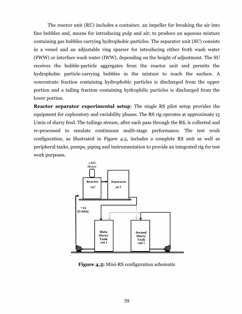
39
The reactor unit (RU) includes a container, an impeller for breaking the air into
fine bubbles and, means for introducing pulp and air; to produce an aqueous mixture
containing gas bubbles carrying hydrophobic particles. The separator unit (SU) consists
in a vessel and an adjustable ring sparser for introducing either froth wash water
(FWW) or interface wash water (IWW), depending on the height of adjustment. The SU
receives the bubble-particle aggregates from the reactor unit and permits the
hydrophobic particle-carrying bubbles in the mixture to reach the surface. A
concentrate fraction containing hydrophobic particles is discharged from the upper
portion and a tailing fraction containing hydrophilic particles is discharged from the
lower portion.
Reactor separator experimental setup: The single RS pilot setup provides the
equipment for exploratory and variability phases. The RS rig operates at approximate 15
l/min of slurry feed. The tailings stream, after each pass through the RS, is collected and
re-processed to emulate continuous multi-stage performance. The test work
configuration, as illustrated in Figure 4.5, includes a complete RS unit as well as
peripheral tanks, pumps, piping and instrumentation to provide an integrated rig for test
work purposes.
.
Figure 4.5: Mini-RS configuration schematic

40
4.3. EXPLORATORY ROUGHER CAMPAIGN
This experimental phase consists on both laboratory and pilot batch testing in
parallel and its main purpose is to identify and define the variables that could already be
frozen as design parameters and which have to remain as variables for the following
phase. Other specific purpose is to select among FWW, IWW or not water at all. The
rougher exploratory campaign covers 60 tests, shown in table 4.5:
Table 4.5: Summary of exploratory rougher tests
Test
Number
Average Grade Variable under exploration
%Cu %Mo %Py
01-20 0.55 0.039 3.7 Interface wash water (IWW)
21-30 0.59 0.040 4.5 Reagents Exploration
31-40 0.53 0.037 4.2 Froth wash water (FWW)
41-50 0.61 0.042 5.3 Slurry density
51-60 0.53 0.032 3.2 Reagents optimization
Experimental measurements: for each pilot run, the following information is
generated and used for the grade/recovery calculations: (i) starting volume of feed slurry
for each run, Vi [m3]; (ii) feed’s fractional solids content CPF at the start of each test using
a Marcy scale; (iii) feed assays, from a dedicated feed sample taken at the beginning of
each test, (iv) concentrate and tails assays for each stage over the duration of the test
and; (v) the mass of concentrate collected for each stage.
Calculation methods for data analysis: the main purpose of above information is
to provide the grade and recovery over the whole test, and at any stage during the test.
There are well-known relationships for the experimental measurements previously
mentioned, based on mass or volumetric balances. Among them, the total starting
volume corresponds to the addition of starting solids volume and starting liquid
volume, thus obtaining:
Vi=HSF
WSF+
(1-CPF)
CPF∙
HSF
WLF (4.1)
And, by definition:
HSF=CPF∙Vi∙WPF (4.2)
Where:

41
HSF : feed solids, in [kg].
CPF : feed’s fractional solids content.
WSF : feed sample dry weight.
WPF : feed sample wet weight.
WLF : feed water weight (water density ~ 1000 [kg/m3].
Therefore, feed solids HSF [kg] is calculated from the measured volume of feed
slurry at the start of each run; the measured feed fractional solids content (from feed
sample wet and dry weights) and; assuming normal conditions for water density.
At steady state, solids shall be balanced:
HSF=HSC+HST (4.3)
As well as volumes shall be balanced at steady state:
HSF
δSF=
HSC
δSC+
HST
δST (4.4)
Concentrate solids over the duration of the run is calculated as follows:
HSC= ∑ HSC,iN1 (4.5)
Where:
HSC, i : mass of concentrate solids at stage i, in [kg].
HSC : concentrate solids collected over the duration of the run, in [kg].
N : number of concentrate samples within a run, twelve (12) in this case.
The Marcy value of CPF is cross-checked against the wet/dry masses of RS feed
sample and it is also back-calculated with the laboratory’s sample dry mass and total
volume. Then, for each stage, several cuts of the tails are taken over the duration of each
stage, and submitted for solids contents and chemical analyses. The overall tails grade
after 12 stages is as recorded from the chemical analysis of the tails sample. Afterwards,
the weight distribution is calculated from the masses of concentrate collected at each one
of the twelve stages of a run, HSC, i. All the concentrate weights are summed, and each
weight is divided by the total weight to give the fractional weight distribution per stage.
WC,i= HSC.i HSC⁄ (4.6)
The chemical assay of the feed sample taken at the beginning of each run is used
as the feed grade of copper and molybdenum. The measured feed grade is compared
with a back-calculated feed grade, just for data verification purposes. The back-
calculated feed grade is calculated as follows:
42
LCu,F,b= (HSC∙LCu,C+HST∙LCu,T) HSF⁄ (4.7)
Where:
LCu, F, b : back-calculated feed grade in %.
LCu, C : combined concentrate assay in %.
LCu, T : tails assay in %.
HSC : concentrate solids collected over the duration of the run, in [kg].
HST : tails solids, in [kg].
HSF : feed solids, in [kg].
Mineral Balance: For each test, the following elemental assays are reported per
sample: Cu; Mo; S and Fe. In addition, CuS is reported per sample as an indication of the
presence of oxide copper species and acid-soluble secondary copper species. Based on
these assays, the following mineral species are accounted for: (i) copper sulphides: the
simplifying assumption is that all copper reports as chalcopyrite (CuFeS2) and calculated
as (Cu ÷ 0.346); (ii) non-sulphide gangue (NSG) is calculated as all mass remaining after
subtracting Cu, Mo, S and Fe. This is based on the assumption that all Cu, Mo, S and Fe
are associated with sulphide species; (iii) Pyrite is accounted for as the remaining mass,
after subtracting sulphide copper and NSG from total mass and; (iv) the following
species (as defined above) are reported in all tables and figures: Cu, Mo, pyrite and NSG.
Non-conventional flotation machines with interface wash water (IWW): The
potential advantage inherent in pulp washing of the high clay feed material is very
important in rougher piloting. The results of four comparisons on the effect of IWW are
shown in figures 4.6 & 4.7. Graphs of copper concentrate grade versus recovery are
provided for Truck 6 (IND-NK), Truck 4 (IND-NK), Truck 1 (NO-IND) and Truck 1 (NO-
IND) samples. As can be seen in figure 4.6, application of IWW is very beneficial for all
comparisons, except the higher grade Truck 1. The application of IWW provided a higher
concentrate grade, but also resulted in higher copper recovery. The increase in
concentrate grade on the rougher is a direct result of increased gangue rejection. Figure
4.7 illustrates this, showing NSG recovery versus copper recovery for the four
comparisons of Figure 4.6. The Truck 1 sample does not show a difference in
performance with the addition of IWW. This suggests that some of the material could
not benefit from wash water. However, it is clear that SE for any of the material with
reasonably high clay levels will be enhanced through the application of IWW.

43
Figure 4.6: Copper grade versus recovery with and without IWW
Figure 4.7: NSG versus copper recoveries with and without IWW

44
In next figure 4.8, RS froth at the first stage can be seen. In the left, before
interface wash water addition; froth appears wet, slimy and dirty. In the right – after
under-froth water addition; froth has rapidly become clean and heavily mineralized.
Figure 4.8: Effect of IWW - left with - right without
Non-conventional flotation machines with froth wash water (FWW):
Adjusting the ring sparser over the froth, FWW is used with Truck 6 and Truck 4
samples. These samples are selected because they have an excellent performance with
IWW. Nevertheless, the results do not show differences in metallurgical performances
with the usage of FWW as can be seen in figure 4.9:
Figure 4.9: Effect of FWW for trucks 4 & 6 (FGU=IND-NK)

45
Slurry density: Truck 6 results at 26-27 % solids are shown in figure 4.10, together
with three additional tests at 31-34 % solids. Concentrate grade is significantly reduced
at higher slurry density, even when IWW is applied. For the Truck 6 material, feed
density needs to be maintained below 30 % solids.
Figure 4.10: Impact of slurry density on copper grade versus recovery for Truck 6
4.4. ROUGHER VARIABILITY CAMPAIGN
This phase of work includes 100 pilot runs for the hypogene ores (tests 6-PP-401
to 500). Materials consisted on 100 variability ore samples, classified into three different
categories: No IND, IND NK and, IND-K. The tests are summarized in Table 4.6.
Table 4.6: Summary of variability campaign ore types
Geologic Group Ore Type # of Tests
HYPOGENE
No IND 43
IND NK 33
IND K 24
The primary objective of this phase is to obtain a significant quantity of
metallurgical data, including RS machine performance on drill core samples; that
represents the hypogene resource, to be applied toward the geometallurgical mine plan.
In parallel with each pilot run, each variability sample is subject to partial extraction
analysis, full ICP analysis, sample characterization test work, QEMScan mineralogy
and a standard Denver bench float test (Denver Seca). As per standard operating
protocol, a Denver float test is performed on the RS feed pulp (Denver Pulp).

46
Samples and initial characterization for variability test work: Prior to the
running of each test in the pilot plant, assay and mineralogical data are given. Having
this information prior to each test is vital to help the team to better read and understand
the flotation performance of each variability sample, and guide for the test operation
accordingly. These responses included adjustments to mass pull, and in few cases,
adjustments to reagent addition. A summary for variability phase test work is shown in
Table 4.7. To gain a clear understanding of the ore body numerous tests are completed
including flotation performance, hardness, density and mineralogy.
Table 4.7: Testing done on variability campaign
Category Test Total
RS and
Denver
RS Pilot Test 100
Pulp Denver Laboratory Test 100
Pulp Denver Laboratory Test with NaHS 8
Dry Denver Laboratory Test 100
Standard
Flotation
MFT 96
Chemical Assays 96
PMA at P80 150 um 96
Parameter Extraction 96
Chemical Assays
Partial Extraction 100
ICP 100
Hardness
SPI 81
Modified BWI 81
Standard BWI 17
Abrasion Test 53
Mineralogy
QEMScan 100
NIR 100
XRD 75
XRD Clay Speciation 25
CEC 25
Density Density 100

47
Procedures and Observations: Each variability sample is delivered as two grounds
and slurred feed charges; each charge of 20.6 kg ground solids as slurry in two buckets,
together with two additional buckets containing process water. The solids plus the
combined water in the four buckets add up to the required solids content for each charge.
The same fixed mass of lime is added to the feed before grinding. Grinding takes
place in a 10kg rod mill. A grind-time is established for each of the variability samples, to
achieve the grind target P80 of 150 µm, based on milling kinetics. The water comes from
a desalination plant, including interface wash water (IWW) and water added to the
laboratory flotation tests over the duration of the tests. In addition, IWW is prepared to
a pH of 10, so as to not cause any significant deviation in the slurry pH over the
duration of a run. Likewise, the water added in lab float tests is also adjusted to pH 10.
Although the pyrite content of all variability samples varies heavily, there is no
protocol to adjust the collector additions into the grinding mill, according to the pyrite
content. Each one of the four buckets per run (two buckets of slurry and two buckets of
water) are weighted before the start of each run, to confirm the feed pulp density. The
actual feed solids content; known at the start of the test by knowing the masses of water
and solids added; and also cross-checked and confirmed through the wet and dry mass
of the feed sub-sample; are the numbers that are reported in this document. All solids
contents arise from wet and dry masses of the samples. Because of the importance of
consistent wet and dry masses for all samples, the tare weights on the sample buckets
are checked and confirmed regularly over the course of this program.
The slurry pH is checked at the start of each test, and adjusted to a standard pH 10
for all tests. In the case of the samples where the ‘as-received’ pH is above 10.25, a small
amount of H2SO4 is used to bring the pH back to the standard pH of 10. Five hypogene
samples are received with a pH above 10 and three of those are above pH 10.25. In all
cases, an initial addition of 25 g/t of frother is added to the pulp prior to extracting the 2L
sample for the Denver lab flotation test; the 2L sample for the feed size distribution
analysis; and the RS feed sub-sample. For all the pilot runs and their corresponding
Denver tests, the frother used is 70:30=X-133: Pine Oil.

48
Analysis: The RS machine performance after 7 stages is compared with Denver Pulp results
after 20 minutes. Figure 4.11 presents the complete body of data (100 tests – 5 culled
results = 95 valid test results), as Cu recovery in the RS after 7 stages versus Cu recovery
in the Denver Pulp test after 20 minutes.
Figure 4.11: Copper Recovery – Denver versus RS
These data clearly fall into three groups: Group A in blue (98 samples) – Delta
Recovery average = 0. Group B in green (8 samples) – Delta Recovery average = 6%.
Group C in red (9 samples) – Delta Recovery average = 26%. Delta Recovery is (Cu
Recovery Pulp, %) – (Cu Recovery RS, %). The blue unity line clearly indicates that for
Group A samples, there is a simple 1-to-1 direct comparison between copper recovery in
the RS (7 stages) and Denver recovery at 20 minutes. Figure 4.12 presents the same data;
this time, plotting mass recovery from the Denver bench test versus feed percent sulfides
(pyrite + copper sulfide).

49
Figure 4.12: Denver Cu Recovery as a function of feed % Sulphides
Group A follows the expected trend, with a slope of about 1.6. Group B shows
mass recovery that is, in general, significantly above the relationship set by the Group A
tests, and the Group C mass recovery is dramatically higher.
The average Denver concentrate grade (for the hypogene samples) for Group A is
3.8 %Cu, versus only 2.1 %Cu for Groups B and 1.8 %Cu for Group C. In other words, for
most of the Group B and C samples, the lab tests were pulled much harder than will
occur in the plant, resulting in very high entrainment levels (average mass recovery for
Group C is 26.6% versus 20.0 for Group B and 12.8% for Group A).
Presenting the data set as Delta copper recovery (Denver - RS) against Delta mass
recovery (Denver - RS), Figure 4.14 confirms that the difference in performance between
the RS and Denver test in Groups B and C can be wholly attributed to the difference in
mass recovery between the two systems.

50
Figure 4.13: Delta Mass Recovery versus Delta Cu Recovery
Should be a key driver towards explaining these divergences in metallurgical
performance (B and C) from the typical performance (A), Table 4-1 considers the Group
C sample characteristics.
Table 4.8: Group C Sample Characteristics

51
As draft analysis, it can be seen that for Group C, the combination of
mineralogical characteristics results in a higher fines proportion in the feed ore, as
quantified by the percent -400mesh fraction, and is shown in Figure 4.15.
Figure 4.14: Delta Recovery versus feed -400 mesh fraction
The specific conclusions from this phase can be summarized as follows: (i) further
analysis of gangue with a potential clustering of clays in families could be very
important; (ii) the results’ analysis focuses on the performance of three groups of
samples, denoted Group A, Group B and Group C; (iii) Group A represents typical
performance of RS accompanying Denver Pulp test. Groups B and C represent divergent
performance, as a result of feed sample mineralogical characteristics.
Regarding the specific application of this chapter, the final conclusion is: “The
non-conventional flotation machine technology is selected together with
interface wash water”.

52
5. PROCESS SIMULATION FRAMEWORK
According to integrated process and control design (IPCD) approach, the process
simulation framework is built upon modelling, simulation and experiments. The
unifying methodology is based on systems identification theory. In this chapter the first
focus is on steady state modelling followed by instrumental setup and ending with
dynamic modelling and implementation.
5.1. SYSTEMS IDENTIFICATION STRATEGY
System identification is a methodology to build dynamic models that has been
mostly applied for data driven box models but it´s now also referred for grey box
models. The aim of system identification is to model systems dynamics that can’t be
easily described using first principles. In next figure 5.1., Ljung’s system identification
iterative work scheme is shown. Formerly used mainly for black box models; nowadays
is utilized also for grey box) models.
Figure 5.1.: System identification iterative work, from Ljung, 1990

53
Construct the experiment and collect the data: the experimental work of this
phase consists mainly on continuous pilot testing. Even though, both laboratory and
pilot continuous testing are run in parallel. Extensive and intensive usages of both off-
line and on-line measurements are executed. By the exception of third party packaged
expert system, all the instruments are tested in this phase. In terms of process control,
the first layer of the control structure is presented in this sub-chapter: instrumentation
and controls. The upper layers of the control structure are presented in chapter 6.
Continuous experimental phase: the main purpose of this campaign is to identify
and implement the process simulation framework and the MPC predictive models for
the control simulation framework. Other specific purposes are: instrumentation startup
and testing and; proportional and integrative (PI) controllers’ tuning. The continuous
campaign covers 122 tests divided in three sub phases as shown in tables 5.1, 5.2 and 5.3:
Table 5.1: Experimental sub phase I: Instrumentation and Control
Test Number Tuned loops and/or instruments
1-8 Cell single loops: level, air flow, wash water flow
9-10 Concentrate area-velocity volumetric flowmeter
11 Volumetric flow meters for feed and tailings
12-15 Feed densitometer
16 Reagents mass flowmeters
17-20 Metallurgical analysers
21-24 Conductivity meters
Table 5.2: Experimental sub phase II: Single RS Cell Characterization
Test Number Name of calibrated and validated model
25-35 Mass and volumetric balance
36-45 Three compartments
46-55 Polat and Chandler – RTD
Table 5.3: Experimental sub phase III: Row Characterization
Test number Description
56-62 Mass and volumetric balance - two (2) cells
63-65 Mass and volumetric balance - three (3) cells
66-70 Mass and volumetric balance - four (4) cells
71-84 RS versus SALA pilot plant (SPP)
85-97 RS versus conventional mini pilot plant (CMPP)
98-122 Variability Testing with three (3) main FGU's

54
Data processing: both data reconciliation and data filtering are considered within
data processing. While both exploratory and variability campaigns are subject to partial
data reconciliation; from here till the end of this thesis, full data reconciliation is done;
either offline and/or online. Matlab routines for offline and online data reconciliation
and parameter estimation are implemented for the purposes of this thesis.
Process model structure selection: the base models, to be adapted and/or
modified and; synthetized in this chapter are: Savassi’s compartmental model; Jämsä-
Jounela dynamic model for pulp levels; Polat & Chandler for collection zone
characterization and; Gorain et al. (2000) and, Bergh & Yianatos (2009) for both
hydrodynamic and kinetic models. In addition to mentioned models, well known mass
balance relationships among control variables are used together for simulation
framework build-up.
Predictive model structure selection: all the predictive models considered in this
thesis, are linear, state space and discrete. When the MPC’s are in profiling mode, they
mutate to adaptive MPC in which case, the models are time variant. In all the other
cases, the models are time invariant. As it is already mentioned in sub chapter 2.5, a
traditional discrete space model representation is used in this thesis, given by equations
(2.35) and (2.36). In the case of adaptive model predictive control, matrices A and B are
time dependant. Regarding the application, three types of MPC’s are developed in this
thesis: (i) row optimizer MPC, MPCR; (2) individual cells MPC’s, MPCn (where n is the
cell number) and; row levels MPC, MPCL. While in case of MPCL the matrices A (t) and
B (t) are symbolic; for MPCR and MPCn, A (t) and B (t) are numerical.
Model fitting strategy: From a high level point of view, it can be hereupon observed
that the cells are over-characterized with the instrumentation available at continuous
experimental phase. The available degrees of freedom are used for parameters’
estimation and data reconciliation. According to the specific experiments and models
under resolution; different parameters are calibrated and validated. As such, the
proportion between degrees of freedom used for parameters’ estimation and those used
for data reconciliation varies. The following model fitting stages are successively
considered: (i) individual cell overall masses and volumes steady state parameters; (ii)
individual zones steady state recoveries; (iii) collection and froth zones models’
parameters; (iv) two, three and four cells rows’ parameters and; (v) “enhanced” Jämsä-
Jounela dynamic model parameters estimations.

55
Model fitting implementation: multiple data sources; including previous
experimental phases such as variability tests and; the continuous experimental phases
described in this chapter; are successfully integrated to maximise both the steady state
and dynamic characterization of the machine-mineral system. Such characterization
details are further explained later on in this chapter, but a brief follows.
Single cell model fitting: the proposed three compartment model has three main
parameters, the corresponding zones recoveries RC, RF and RQ; well determined,
reconciled and validated by the experimental data as well as the total recoveries RRS or
RCONV. While collection zone recoveries obtained from three compartmental model
fitting, are tested and compared against Polat & Chandler model fitting; both froth and
quiescent recoveries are kept as obtained from three compartmental fitting.
Collection zone model fitting: the assumption that the collection sub-process
happens only within the reactor unit is used and tested. While kinetic characterization
is done using parallel batch tests, residence time distribution parameters are
experimentally determined for both the reactor unit and the whole RS machine,
through conductivity testing in both RS’s compartments. For RS machines as well as for
conventional ones, comparisons are done between results from Polat & Chandler
parameters’ fitting and three compartmental RC fitting.
Row model fitting is related to grades and recoveries obtained from both cell-based
and row-based manipulated variables. Regarding row-based controlled variables
(reagents), model fitting is based on data driven models. Also, as the startup dynamic
model (Jämsä-Jounela) is row based, the dynamic model structure and fitting is
described within the row characterization sub-chapter.
Dynamic model fitting: Experimental input signals need to be designed with few
basic properties, to extract informative dynamical response from the process. The main
idea for performing dynamic model fitting tests is to design input signals which: are
rich enough to reveal the system dynamics; let the system perform around nominal
operating points and; are chosen according to the bandwidth of expected dynamics.
Models’ validation: All the estimated models are validated with independent data
sets. The validation data set is pre-processed in the same way as the estimated data set.

56
5.2. INSTRUMENTATION AND CONTROL
Single cell measurements and basic controls: each cell “n” has the following
basic control loops: pulp level control loop (LIC-n1); air control loop (FIC-n1) and;
interface wash water control loop (FIC-n2). Next figure 5.2 shows the basic
instrumentation and controls of each cell using ISA 95 standard. FT-03 is a concentrate
volumetric flow transmitter.
Set points (SP) could be either managed independently by the operator or could
be manage by the levels’ MPC in case of level control loops or; “Cell n” MPCn in case of
both wash water and air flows. MPC’s are described in chapter 6, as well as all the other
components of the control structure.
Figure 5.2: Cell n instrumentation and basic control scheme
Pulp level control loop - LIC-n1 - contains a modulating knife gate valve and a
magnetostrictive double float / double level measuring unit. The first float sits at the
froth/slurry interface – “LE-n1” - and the second float sits on top of froth – “LE-n2”.-.
This loop is managed by a PI controller, but its set point is stablished either by the
operator or by the MPC that controls all the levels along the row (MPCL). LE-n1
represents the pulp level and LE-n2 represents froth height over the lip and is
afterwards used for the supervisory purposes described in chapter 6.
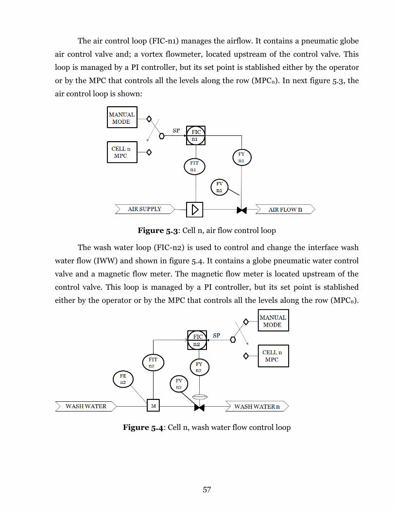
57
The air control loop (FIC-n1) manages the airflow. It contains a pneumatic globe
air control valve and; a vortex flowmeter, located upstream of the control valve. This
loop is managed by a PI controller, but its set point is stablished either by the operator
or by the MPC that controls all the levels along the row (MPCn). In next figure 5.3, the
air control loop is shown:
Figure 5.3: Cell n, air flow control loop
The wash water loop (FIC-n2) is used to control and change the interface wash
water flow (IWW) and shown in figure 5.4. It contains a globe pneumatic water control
valve and a magnetic flow meter. The magnetic flow meter is located upstream of the
control valve. This loop is managed by a PI controller, but its set point is stablished
either by the operator or by the MPC that controls all the levels along the row (MPCn).
Figure 5.4: Cell n, wash water flow control loop

58
Row instrumentation - direct measurements: For each stream (F: feed, C:
concentrate, T: tailings), there is an on-line XRF metallurgical analyzer that delivers
copper, molybdenum, iron and arsenical grades, together with solids percentage CP.
Copper and molybdenum grades (LCu,F, LMo,F, LCu,C, LMo,C, LCu,T, LMo,T) are used by the
optimization layer after being subject to on-line data reconciliation using iron and
arsenical grades (LFe,F, LAs,F, LFe,C, LAs,C, LFe,T, LAs,T). In addition, on-line volumetric
flowmeters deliver the corresponding measurements QF, QC and QT. While the
volumetric flowmeter for feed is magnetic, the other two ones are area-velocity ones.
Additionally, the feed pulp density (δPF) is measured by means of an electro-
tomography instrument (non-radioactive). Finally, mass flowmeters (Gi) are available
for the following reagents: lime, primary and secondary collector and, frother blend. In
next figure 5.5, row measurements are shown, where X represents Cu, Mo, Fe and
Arsenic; and i represents lime, primary collector, secondary collector and frother blend.
Figure 5.5: Row instrumentation

59
5.3. SINGLE CELL CHARACTERIZATION
Compartmental model synthesis: as mentioned in sub chapter 2.3, Savassi’s
compartmental model has two compartments regarding “true flotation”: collection zone
and froth zone and, can be represented by figure 5.6 and equation 5.1:
Figure 5.6: Two compartment model (adapted from Savassi, 2005)
Rtot=Rc,i∙Rf,i
1 - Rc,i∙(1 - Rf,i) (5.1)
Where,
Rtot : Total cell recovery due to true flotation
Rc, i : Collection recovery of specie i
Rf, i : Froth recovery of specie i
[Fi] : Feed solids flow
[Ci] : Concentrate solids flow
[Ti] : Tailings solids flow
Specie i could be water, gangue particle, valuable particle or mixed particle.
Additionally, either dynamic or steady state analysis can be done if dynamic mass
accumulation is considered for each compartment.
A full three compartmental approach is proposed in this thesis. With Rq,i
representing quiescent zone recovery of specie i; the models of both conventional RS
cells; are correspondingly shown in figures 5.7 and 5.8:

60
Figure 5.7: Full three compartmental model of conventional mechanical cell
Figure 5.8: Full three compartmental model of a RS flotation machine
Then, the total recoveries for specie “i” in a conventional cell (Rconventional) and in
a RS machine (RRS); can be expressed by:
Rconventional=Rc,i∙Rq,i∙Rf,i
1 - Rc,i∙(1-Rq,i) - Rq,i∙(1 - Rf,i
) (5.2)
RRS,i=Rc,i∙Rq,i∙Rf,i
1 - Rq,i∙(1 - Rf,i
) (5.3)
It can be noticed that; if the zone recoveries were the same, the recovery of the
conventional machine would be bigger. This structural difference is due to the fact that
in case of RS flotation machine, particles detached in the separator tank report to the
tailings because they do not have the probability return to the RU to be collected again.

61
Mass balance experimental synthesis: As part of the integrated process and
control design (IPCD) approach, both cell layer and row layer instrumentation are
available for pilot cell characterization. All of them are herein successively used for one
cell, two cells and the entire row of four cells. Next figure 5.9, shows row layer’s
instrumentation applied to one cell characterization. It represents a model by itself,
herein called “single cell – row model” (SCRM). While SCRM is presented here,
“double cell – row model” (DCRM) and “multiple cell – row model” (MCRM) are
presented in next sub-chapter.
Figure 5.9: Single cell row direct measurements applied to one cell
Correspondingly, synthetizing the SCRM with the proposed three compartment
model, the following figures 5.10 and 5.11 arise for conventional and RS cells:
Figure 5.10: SCRM + conventional cell three compartment model

62
Figure 5.11: Single cell row model + RS three compartment model
At steady state, the following equations are used for resolving parameters Rq , Rf
and Rc for each one of both types of cells: one (1) recovery equation (5.4 or 5.5); four (4)
mass pulls obtained from (5.15); one (1) recovery (Cu) from (5.14) and; the mentioned
4x4 system given by equations (5.4), (5.5), (5.11) and (5.12). As can be observed, three
degrees of freedom are needed from six available. Then, three degrees of freedom are
available for: data reconciliation and; instruments’ validation. While cells’ parameters
from vendors are shown in table 5.4; three compartmental models fitting results are
presented in tables 5.5 and 5.6. Number of cells and row residence times are shown only
for context and for reference afterwards in this thesis.
Table 5.4: Cells’ operational parameters
Cell type Cells # Cell Volume Pulp flow τROW min τCELL min
RS (*) 4 15/45 l ≈15 l/h ≈4/12 ≈1/3
ERIEZ 3 1.7 l 16.2 l/h 15.5 – 17.0 5.2 - 5.7
SALA 8 80 l 0.86 m3/h 37.4 - 38.1 4.7 - 4.8
(*) In the case of RS machines, there are two values for volume, flow and
residence times: reactor unit parameters and, entire RS machine ones.

63
Table 5.5: RS three compartmental model fitting
RRS
RC RF RQ Experimental R2 Theory
HYPF-01 0.807 0.577 0.732 0.503 0.922 0.494
HYPF-02 0.806 0.553 0.701 0.472 0.934 0.455
HYPF-03 0.794 0.557 0.698 0.463 0.907 0.447
Average 0.804 0.564 0.717 0.485 - 0.464
Table 5.6: RS versus conventional three compartmental model fitting
RTOTAL
RC RF RQ Experimental R2 Theory
SALA 0.709 0.450 0.513 0.444 0.831 0.439
ERIEZ 0.759 0.406 0.601 0.558 0.844 0.544
RS 0.804 0.564 0.717 0.485 >0.907 0.464
As first insight, it can be observed that: (i) the RS model fitting shows better
fittings (R2) than conventional cells; (ii) even though, RS residence times are
considerable smaller, total recoveries are not so different; (iii) RS zone recoveries are
bigger than conventional cells’ zone recoveries but, as an structural effect of direct
reporting to tailings (figures 5.7 & 5.8, equations 5.2 & 5.3), RS total recoveries are
smaller; (iv) almost always, experimental total recoveries are greater than theory and;
(v) among zone recoveries, the collection zone shows better adjustment.
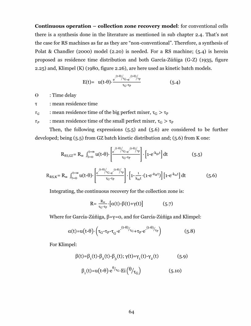
64
Continuous operation – collection zone recovery model: for conventional cells
there is a synthesis done in the literature as mentioned in sub chapter 2.4. That’s not
the case for RS machines as far as they are “non-conventional”. Therefore, a synthesis of
Polat & Chandler (2000) model (2.20) is needed. For a RS machine; (5.4) is herein
proposed as residence time distribution and both García-Zúñiga (G-Z) (1935, figure
2.25) and, Klimpel (K) (1980, figure 2.26), are here used as kinetic batch models.
E(t)= u(t-θ)∙e
-(t-θ)
τG⁄
-e-(t-θ)
τP⁄
τG-τP (5.4)
ϴ : Time delay
τ : mean residence time
𝜏𝐺 : mean residence time of the big perfect mixer, τG > τP
𝜏𝑃 : mean residence time of the small perfect mixer, τG > τP
Then, the following expressions (5.5) and (5.6) are considered to be further
developed; being (5.5) from GZ batch kinetic distribution and; (5.6) from K one:
RRS,GZ= R∞ ∫ u(t-θ)∙ [e
-(t-θ)
τG⁄
-e-(t-θ)
τP⁄
τG-τP] ∙ [1-e-kgzt]
t=∞
t=0dt (5.5)
RRS,K= R∞ ∫ u(t-θ)∙ [e
-(t-θ)
τG⁄
-e-(t-θ)
τP⁄
τG-τP] ∙ [1-
1
kmt∙(1-e-𝑘𝐾t)] [1-e-kmt]
t=∞
t=0dt (5.6)
Integrating, the continuous recovery for the collection zone is:
R= R∞
τG-τP∙[α(t)-β(t)+γ(t)] (5.7)
Where for García-Zúñiga, β=γ=0, and for García-Zúñiga and Klimpel:
α(t)=u(t-θ)∙ (τG-τP-τG
∙e-(t-θ)
τG⁄
+τP∙e-(t-θ)
τP⁄
) (5.8)
For Klimpel:
β(t)=β1(t)-β
2(t)-β
3(t); γ(t)=γ
1(t)-γ
2(t) (5.9)
β1(t)=u(t-θ)∙e
θτG
⁄ ∙Ei (θτG
⁄ ) (5.10)

65
β2(t)=u(t-θ)∙ (e
θτG
⁄ ∙Ei(tτG
⁄ )-eθ
τP⁄ ∙Ei(t
τP⁄ )) (5.11)
β3(t)=u(t-θ)∙e
θτP
⁄ ∙Ei (θτP
⁄ ) (5.12)
γ1(t)=u(t-θ)∙ [e
θτG
⁄ ∙ (Ei (θ∙(Km∙τG+1)
τG⁄ ) -Ei (
t∙(Km∙τG+1)τG
⁄ ))] /Km (5.13)
γ2
(t)=u(t-θ)∙ [eθ
τP⁄ ∙ (Ei (
θ∙(Km∙τP+1)τP
⁄ ) -Ei (t∙(Km∙τP+1)
τP⁄ ))] /Km (5.14)
It can be commented that even though above symbolic expressions are
manageable for a single cell, that’s no appear to be true for a row of RS machines. In
this thesis, these formulas are not used for a row; but it’s worth the effort to herein
suggest the usage of numerical methods for that case.
Collection zone experimental work: while kinetic constants are obtained from
variability campaign, residence time distributions (RTD) shall be experimentally
obtained. In following figures 5.12 and 5.13, the experimental schemes are presented:
Figure 5.12: Experimental setup for conventional machine RTD

66
Figure 5.13: Experimental setup for RS machine RTD parameter fitting
Collection zone residence time experimental procedure: RTD tests are
performed for RS machines. A brief description of the test follows:
(i) Installation of conductivity electrodes in the column and subsequent connection of to
a signal adapter system. Then, the signal adapter system to a data acquisition card
embedded in a notebook that has data acquisition software.
(ii) Conditioning of 72 liters of pulp, 2 kg of fine salt and 500 cm3 of 0.2 M hydrochloric
acid into the "Conductive Pond".
(iii) Starting the pumping together with data acquisition → export of data generated by
to Excel → import of data from Excel to MATLAB → reconciliation of experimental data
→ model fitting through script routines.
Collection zone residence time results are shown in following tables 5.7 and 5.8.
All the tests are performed with the same material (truck 4) for the same FGU. In table
5.7, the LTST (large tank – small tank) model (Yianatos et al., 2007c) is used for
conventional SALA cells. Then, in table 5.8, the real mixer model is used for fitting the
residence time distribution of the reactor unit and; the herein proposed model (5.4) is
used for fitting the residence time distribution of the entire RS machine. The estimator
R2 is shown as adjustment quality index.

67
Table 5.7: Conventional SALA cells’ RTD model fitting (time in seconds)
Test 48 Test 49 Test 55 τtheory
HYPF1 HYPF1 HYPF1 VT/Q
τG [s] 203.44 209.82 205.32 -
τP [s] 37.65 43.16 46.55 -
τ [s] 241.09 252.98 251.87 284.47
R2 0.90 0.89 0.88 -
From table 5.7, it can be noticed that the total fitted time residence is less than
the “actual” residence time, calculated by the ratio between total volume and flow. That
result is logical and it’s commonly related to 2 problems: short circuits and/or material
that remains a lot of time in the reactor occupying the place of fresh feed. Regarding the
quality of the adjustment, R2 is good enough.
Table 5.8: RS-RTD model fitting
Test 47 Test 50 Test 53 τtheory
T_47a T_47b T_50a T_50b T_53a T_53b VRU/Q VT/Q
τ [s] 57.89 162.22 57.27 158.70 57.55 160.70 61.20 183.60
τG [s] - 118.73 - 116.10 - 117.20 - -
τP [s] - 58.37 - 55.90 - 56.30 - -
ϴ [s] 2.92 5.21 3.08 6.30 3.17 7.40 - -
R2 0.93 0.91 0.94 0.92 0.93 0.92 - -
From table 5.8, it can be observed that the reactor unit adjustments give smaller,
but very similar times than the ratio between the reactor unit volume and the flow. Also,
all the adjustments have good quality indices.
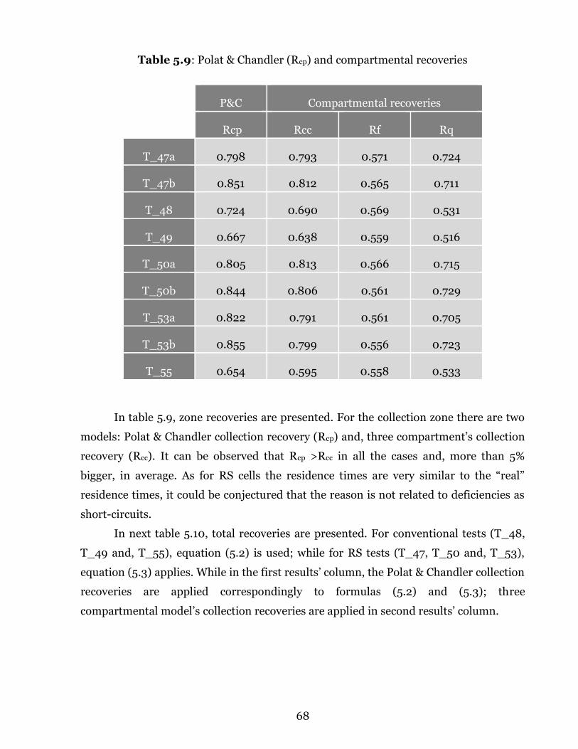
68
Table 5.9: Polat & Chandler (Rcp) and compartmental recoveries
P&C Compartmental recoveries
Rcp Rcc Rf Rq
T_47a 0.798 0.793 0.571 0.724
T_47b 0.851 0.812 0.565 0.711
T_48 0.724 0.690 0.569 0.531
T_49 0.667 0.638 0.559 0.516
T_50a 0.805 0.813 0.566 0.715
T_50b 0.844 0.806 0.561 0.729
T_53a 0.822 0.791 0.561 0.705
T_53b 0.855 0.799 0.556 0.723
T_55 0.654 0.595 0.558 0.533
In table 5.9, zone recoveries are presented. For the collection zone there are two
models: Polat & Chandler collection recovery (Rcp) and, three compartment’s collection
recovery (Rcc). It can be observed that Rcp >Rcc in all the cases and, more than 5%
bigger, in average. As for RS cells the residence times are very similar to the “real”
residence times, it could be conjectured that the reason is not related to deficiencies as
short-circuits.
In next table 5.10, total recoveries are presented. For conventional tests (T_48,
T_49 and, T_55), equation (5.2) is used; while for RS tests (T_47, T_50 and, T_53),
equation (5.3) applies. While in the first results’ column, the Polat & Chandler collection
recoveries are applied correspondingly to formulas (5.2) and (5.3); three
compartmental model’s collection recoveries are applied in second results’ column.

69
Table 5.10: Total recoveries and errors related to experimental results
Total recoveries Recoveries’ errors %
w/Rcp w/Rcc Experimental w/Rcp w/Rcc
T_47a 0.479 0.476 0.455 5.32 4.66
T_47b 0.494 0.472 0.445 10.98 5.90
T_48 0.507 0.483 0.460 10.17 4.94
T_49 0.428 0.410 0.404 6.12 1.48
T_50a 0.472 0.477 0.465 1.44 2.45
T_50b 0.508 0.485 0.485 4.76 0.05
T_53a 0.470 0.453 0.451 4.24 0.32
T_53b 0.506 0.473 0.449 12.66 5.29
T_55 0.424 0.386 0.380 11.48 1.40
Regarding RS tests, it can be noticed that the collection recoveries obtained from
the three compartmental models, have considerable smaller errors than the recoveries
calculated using P&C. Nevertheless, it’s worth to mention that the P&C collection
recoveries used are the ones from the proposed model, not using the simpler “real
mixer” model for reactor unit. In that case, the error is smaller and that can be seen
observing that the residence times of the reactor unit obtained by DTR’s are very similar
to the “real” ones. In practical terms, conductivity measurements are recommended
herein in the reactor unit compartment.
For conventional tests (T_48, T_49 and, T_55), it can also be observed that the
collection recoveries obtained from the three compartmental models, have considerable
smaller errors than the recoveries calculated using P&C. But, from table 5.8 it can be
noticed that the fitted residence times are around ten percent smaller than the “real”
residence times calculated by means of the ratio between volume and flow.

70
5.4. ROW CHARACTERIZATION
Next figures 5.13, 5.14 and 5.15 show row layer’s instrumentation applied
successively to two, three and four cells row characterization. They represent models by
themselves, related mainly to masses and volumes balances.
Figure 5.13: Double cell row model
Figure 5.14: Triple cell row model
Figure 5.15: Four cell row model
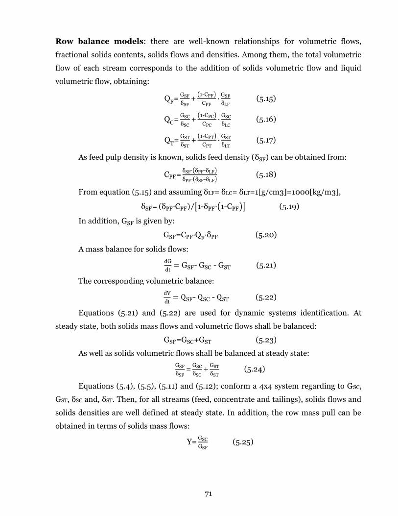
71
Row balance models: there are well-known relationships for volumetric flows,
fractional solids contents, solids flows and densities. Among them, the total volumetric
flow of each stream corresponds to the addition of solids volumetric flow and liquid
volumetric flow, obtaining:
QF=
GSF
δSF+
(1-CPF)
CPF∙
GSF
δLF (5.15)
QC
=GSC
δSC+
(1-CPC)
CPC∙
GSC
δLC (5.16)
QT=
GST
δST+
(1-CPT)
CPT∙
GST
δLT (5.17)
As feed pulp density is known, solids feed density (δSF) can be obtained from:
CPF=δSF∙(δPF-δLF)
δPF∙(δSF-δLF) (5.18)
From equation (5.15) and assuming δLF= δLC= δLT=1[g/cm3]=1000[kg/m3],
δSF= (δPF∙CPF) [1-δPF∙(1-CPF)]⁄ (5.19)
In addition, GSF is given by:
GSF=CPF∙QF∙δPF (5.20)
A mass balance for solids flows:
dG
dt= GSF- GSC - GST (5.21)
The corresponding volumetric balance:
dV
dt= QSF- QSC - QST (5.22)
Equations (5.21) and (5.22) are used for dynamic systems identification. At
steady state, both solids mass flows and volumetric flows shall be balanced:
GSF=GSC+GST (5.23)
As well as solids volumetric flows shall be balanced at steady state:
GSF
δSF=
GSC
δSC+
GST
δST (5.24)
Equations (5.4), (5.5), (5.11) and (5.12); conform a 4x4 system regarding to GSC,
GST, δSC and, δST. Then, for all streams (feed, concentrate and tailings), solids flows and
solids densities are well defined at steady state. In addition, the row mass pull can be
obtained in terms of solids mass flows:
Y=GSC
GSF (5.25)

72
From grades measurements, the following information is obtained: row
metallurgical recoveries and row mass pulls:
RX=LX,C∙(LX,F-LX,T)
LX,F∙(LX,C-LX,T)=
LX,C∙GSC
LX,F∙GSF (5.26)
YX=(LX,F-LX,T)
(LX,C-LX,T)=
GSC
GSF (5.27)
Where sub index “X” can represent Mo, Cu, Fe or As.
Then, five mass pulls are available, four from equation (5.26) and one from
equation (5.25). As mass pulls shall be equal, four mass pulls are available for
additional variables resolution and/or data reconciliation, as it is further explained
wherever applies. Now, it can be said that degrees of freedom are used in the following
section for dynamics’ estimation.
Dynamic models synthesis: as mentioned in sub chapter 2.3, Kämpjärvi & Jämsä-
Jounela dynamic model is selected as “startup model”. In this sub chapter, some
simplifications of the mentioned model are taken out. Here, there is interface wash water
(IWW) flow and a concentrate flow. Additionally, pulp densities do vary along the row.
Also, there is a volumetric air holdup (Εg). Therefore, instead of equation (2.4), the
following equation (5.28) applies for each cell along the row; considering that: QW,i and
Εg,i are correspondingly, the interface wash water and the volumetric gas holdup of cell i:
dVi
dt= Q
Fi- Q
Ci - Q
Ti+ Q
Wi+ Eg,i (5.28)
It’s important to mention that herein the air holdup is not in percentage, but it is
considered as volumetric gas holdup.
From (5.21) & (5.22) & (5.23), for cell i:
dGi
dt= GSFi- GSCi - GSTi (5.29)
For dynamic balances of valuable solids contents:
dGX,i
dt= GSF,X,i − GSC,X,i − GST,X,i (5.30)
Then, considering that Qin is feed flow; S is the area; c is the physical difference
in height between the cells; K is a constant coefficient; Cv is the valve coefficient, given
by valves’ vendor and; yi, ui are respectively, the pulp level and control signal of cell i:

73
dy1
dt=
QF1
S-
QC1
S -
K
SCv(u1)√𝛿1y1 − 𝛿2 ∙ (y2 − c)+
QW1
S+
Eg1
S (5.31)
dy2
dt=
K
SCv(u1)√𝛿1y1 − 𝛿2 ∙ (y2 − c)-
K
SCv(u2)√𝛿2y2 − 𝛿3 ∙ (y3 − c)-
QC2
S+
QW2
S+
Eg2
S (5.32)
dy3
dt=
K
SCv(u2)√𝛿2y2 − 𝛿3 ∙ (y3 − c) −
K
SCv(u3)√𝛿3y3 − 𝛿4 ∙ (y4 − c)-
QC3
S+
QW3
S+
Eg3
S (5.33)
dy4
dt=
K
SCv(u3)√𝛿3y3 − 𝛿4 ∙ (y4 − c) −
K
SCv(u4)√𝛿4y4-
QC4
S+
QW4
S+
Eg4
S (5.34)
A symbolic process simulator is implemented. It’s based on a library of
configurable functions with symbolic parameters linearized around symbolic operating
points. The linearization is the traditional. If state space derivative vector is defined as:
Ẋ = G(X, U) (5.35)
If Ŷ and Ŵ, are the operating points column vectors inputs and outputs:
Ẋ = F(Y, W) − F(Ŷ, Ŵ) (5.36)
Applying Taylor’s first order approximation:
Ẋ = ∇F (Y; (Ŷ, Ŵ)) ∙ (Y − Ŷ) + ∇F (W; (Ŷ, Ŵ)) ∙ (W − Ŵ) (5.37)
Where, Y is the column vector of pulp levels; W is the column vector of control
signals; F is the column vector of pulp level derivatives, X=Y- Ŷ, U=W-Ŵ, and ∇F(Y ;( Ŷ,
Ŵ)) and ∇ F (W ;( Ŷ, Ŵ)) are the correspondingly Jacobeans evaluated in the operating
point. The objective is to obtain state space matrices A, B, C, D and E; for both process
simulation and for predictive model building. Regarding predictive models, one set of
state space matrices are needed for each one of the MPC’s. For pulp levels MPC, MPCL
and, for individual cell MPC, MPCn; matrices A and B are symbolic. Matrices C and D
are data driven for all the MPC’s.
Regarding pulp levels process simulation blocks, pulp level control valves used
for this work are a special type of knife gate valves for control applications with special
seat plates. The inherent characteristic is a compromise between equal percentage &
linear flow characteristics. From the vendor technical specifications, Cv (w) relation is
obtained where Cv is the valve coefficient and w the control signal, both normalized
from 0 to 1.

74
Non-zero elements of A, B are shown in equations (5.38) to (5.47). For first row:
A(1,1) =−KCv(w1)
2S√c+y1−y2 , A(1,2) =
KCv(w1)
2S√c+y1−y2 (5.38)
For intermediate A components, 1 < i < n and, then:
A(i, i − 1) =KCv(wi−1)
2S√c+yi−1−yi (5.39)
A(i, i) = −KCv(wi−1)
2S√c+yi−1−yi−
KCv(wi)
2S√c+yi−yi+1 (5.40)
A(i, i + 1) =KCv(wi)
2S√c+yi−yi+1 (5.41)
For i=n:
A(n, n − 1) =KCv(wn−1)
2S√c+yn−1−yn (5.42)
A(n, n) = −KCv(wn)
2S√yn−
KCv(wn−1)
2S√c+yn−1−yn (5.43)
The first row of B matrix is given by:
B(1,1) =−K
d𝐶𝑣dw
(w1)√c+y1−y2
S (5.44)
While for 1<i <n, then:
B(i, i − 1) =K∙
d𝐶𝑣dw
(wi−1)√c+yi−1−yi
S (5.45)
For i=n:
B(n, n − 1) =K
d𝐶𝑣dw
(wn−1)√c+yn−1−yn
S (5.46)
B(n, n) =−K
d𝐶𝑣dw
(wn)√yn
S (5.47)
Other predictive models’ descriptions are done in next chapter.

75
6. ADVANCED CONTROL AND OPTIMIZATION
6.1. ADVANCED CONTROL PERSPECTIVE
The problem addressed in this chapter is the need of further approaches that can
provide both powerful and integrated solutions for advanced process control and
optimization of flotation plants. The solution proposed in this study is a hierarchical
and dynamic approach that takes advantage of available powerful techniques in the
family of model predictive control algorithms together with cutting edge or novel
instrumentation systems.
Until nowadays, the attitude at flotation plants has commonly been in the
comfort zone due to former wealthy period. That unambiguously determines the need
for more productivity and efficiency in the use of available resources.
Traditionally, process design and control design are strictly sequential tasks. The
process is designed first to achieve the design objectives, and then, the operability and
controllability aspects are considered through control design. This sequential approach
is often inadequate since many process control challenges arise because of poor design
of the process and may lead to overdesign of the process, dynamic constraint violations,
and may not guarantee the required performance (Malcom et al., 2007).
As discussed by Edgar (2004), the priorities of the objectives have been reversed.
In the early approaches, the control system was simply a tool to achieve the
predetermined goals of production, which had been set in the process design stage. The
operation personnel did not think of the control system as an optimization tool to
improve profitability of the process. Therefore, economic optimization had the lowest
priority. However nowadays, business planning of process industries has become online
and much less limited by the early decisions at the design stage. Consequently, the new
control systems have also inputs in terms of economic parameters and translate them
into operational decisions. This has encouraged designers to consider the highest
priority to process profitability and the roles of other control tasks are to realize the
targeted economic objectives. In spite of the fact that economics are not under the scope
of this work, the hierarchical approach based in temporal decomposition, give the
needed and enough time for management decision making integrating both technical
and commercial aspects.

76
6.2. ADVANCED CONTROL METHODOLOGY
Model-base design is the systematic and methodological approach for the whole
work presented in this chapter. As such, the methodology framework includes specific
model-base methods for: (i) process control design, (ii) control simulation framework
implementation (ii) process modelling and,. Process models are the base for both the
simulation of the process and, the controllers’ implementation. Also, the main objective
of this chapter is froth flotation control. Then, the model framework shall emulate the
froth flotation process with needed and enough precision for process control purposes
In terms of process control, the model framework shall represent the relationship
between the measured, controlled and manipulated variables in order to achieve the
control objectives in spite of measured or unmeasured disturbance variables. This
article is entirely model-based, including the control strategies. As such, both process
simulator sub system and controller simulator sub-system are built upon an
appropriate and comprehensive selection and synthesis of existing first principle
models (white box), data driven models (black box) and/or a combination of both (grey
box). It’s important to state that both process and prediction models for control
implementation, are calibrated and validated using pilot and/or industrial data. From a
process control perspective, while process simulation framework is open loop, control
simulation framework is closed loop. Then, the process simulator is used for both
process simulation and controller implementation and; the control simulator is used to
test control strategies by simulation without full closed loop experimental calibration or
validation. That´s in the essence of model and simulation based methodologies: there
could be a simulation framework without full experimental background, as long as the
thoroughness and rigor, for the moment to arrive at the conclusions, is preserved.
Regarding simulation framework implementation, the methodology used to
incrementally and systematically merge and combine first-principle models and
empirical models in a comprehensive simulation framework is mainly based on Ljung’s
systems identification book (1990).

77
6.3. CONTROL DESIGN
Conceptual control design includes the following definitions: degree of
centralization; control hierarchy; control structure and; set point policy.
Degree of centralization: An approach between pure decentralized and full
centralized is used herein. Specifically, a cooperative control structure is selected for
this thesis because while neither a pure decentralized control structure nor a
communicated one ensures an optimal operation, there are many concerns reliability
and maintainability of a large-scale centralized control structure. A cooperative control
structure employs an objective function for the whole system, and the prediction of the
last iteration of each controller is available to the others.
Control Hierarchy: A fit for purpose three layered hierarchy is used in this work.
Also, the control structure is decentralized vertically (top-down) through different time
scales, that can varies upon certain states that are later described in this article: (i) a
daily (24 h) or shift (8h) basis for orchestrator’s changes in given technical optimum
criterion and constraints; (ii) an hour basis for row orchestrator outputs to lower levels
(set points or overriding); (iii) a ten minutes’ basis for advanced control and (iv) a one
to ten seconds of sampling time for basic control. Regarding the dynamic approach of
the hierarchy, depending on the mode (tracking or regulatory) and/or the variable
being profiled, the three-layer hierarchy can vary it behavior. Next figures show the
three layered row control hierarchy, presenting the main components. The technical
optimum criteria can be biased and/or weighted according to economics.
Figure 6.1: Row control hierarchy
In next figures (6.2) and (6.3) the advanced control layer is firstly presented in
the form of schemes, being (6.2) the advanced control for a cell and (6.3) the advanced
control schema for a row.

78
Figure 6.2: Cell-based advanced control scheme
Figure 6.3: Row based advanced control scheme
79
As can be seen in previous figures, the advanced control layer is composed of
MPC’s: n cells’ MPCs, MPCn; 1 MPC for all the pulp levels of a row, MPCL; 1 MPC for
three reagents (Rg1, Rg2, Rg3) and; 1 MPC for ph advanced control with the capability
to act as a Eh controller in addition to ph.
The hierarchical control structure considers three layers: orchestrator, advanced
control and regulatory control. The orchestrator layer plays two main roles: supervision
and optimization. In previous figure 6.2, the row orchestrator is shown receiving and
transmitting information with MPCL, MPCn and the third party expert system.
Control Structure: Skogestad’s (2004) iterative top-down/bottom-up algorithm is
used as control structures’ selection methodology. Nevertheless, the bottom-up
approach is used to present the work because both experiments and simulations are
developed in a bottom-up sequence.
Regarding measurements, state of the art, cutting edge and new instrumentation
systems are used at pilot trials. Among them: (i) magnetostrictive multi-level sensor
that measures both pulp level and top of froth depth level, (ii) concentrate volumetric
flow by means of area-velocity instruments, (iii) image processing system, (iv) linear
knife-characterized control valves, (v) mass flow meters, (vi) tomography density
meters and, (viii) online metallurgical analyzers. Also in the first layer of the control
structure, the manipulated variables are valves and the controlled variables are flows.
The control objective of the first layer is to keep the controlled variables closer to the set
points within a certain actuation effort. In other words, the performance or cost
function to be minimized is a tradeoff between error and effort.
The following basic control loops and measurement systems are available for
each mechanical cell (where n is the cell number): air control loop (FIC-n1), interface
wash water control loop (FIC-n2) and, pulp level control loop (LIC-n1). These basic
control loops are described in previous chapter 5. Each of them has their own dynamic
behaviors, not considered for advanced control and optimization layers applying
temporal decomposition. This seems right, as far as the time responses from the
measurements to the valves are at least one order of magnitude faster than the
advanced control time constants.

80
Row-based control loops are considered for collector, frother and milk of lime.
These reagents are measured by means of Coriolis mass flowmeters and the
manipulated variables are positive displacement dossing pumps.
The following indirect instrumentation is considered for each cell: froth expert
system (AIC-nm, m variables per cell); froth stability sensors (two per cell); concentrate
mass pull virtual sensor and; concentrate grade virtual sensor (LCu, C, b; one per cell).
The second layer of the control structure – advanced control – is where MPC’s
live (by the exception of row optimizer MPC, MPCO). The manipulated variables
considered herein are froth depth, wash water, air flow, frother, collectors and milk of
lime. The controlled variables of the second layer are grades and recoveries. The
technical optimum is configurable, as well as performance indices or cost functions.
The orchestrator is composed by two sub systems: optimizer and supervisor. The
optimizer is MPC-based, called herein MPCO. The orchestrator’s role in the
optimization of a row performance is to achieve the given requirements. It determines a
optimum set points for the controllers. Related to the supervisory role, the following
virtual sensors are developed: (i) froth instability, (ii) sunken or pulping cells and, (iii)
individual mass pulls and concentrate grades. In addition, the orchestrator monitors,
maintains and set the mode of lower control layers and instrumentation; enunciating if
they are not performing to expectations. Once the plant has reached stability, the
orchestrator turns to be mainly an optimizer while maintaining its supervisory tasks.
Regarding both supervisor and optimizer, froth stability is a key factor for
feasibility and optimality. Stable operation of flotation cells and consequent consistent
metallurgical benefits can only be obtained if pulp levels and froth stability are under
control. Froth flotation process depends on a carefully controlled and stable froth. In
this work, two indices for froth stability are used. Next figure 6.4 shows expert system
scheme together with froth stability observers and associated signals. The froth expert
system is a packaged image processing system that delivers the following automatic
measurements: froth velocities, bubble size distribution and concentrate grade
estimation.

81
Figure 6.4: Cell n froth stability observers
Row optimizer: from a top-down perspective, Maldonado et al. (2011) find that the
maximum separation efficiency is obtained when each of the cells along the row has the
same recovery if entrainment is not considered. Singh and Finch (2014) confirmed that
with simulations and industrial flotation. In the same article, they used mathematics
and simulations to propose that, considering gangue entrainment, “a balanced mass-
pull profile would be the optimal policy”. Seguel et al. (2015) revisit row optimization
through froth depth profiling using a genetic algorithm and the following formulation of
the optimization problem: maximization of the overall Cu recovery while satisfying a
minimum concentrate grade. One of their conclusions is that optimal profile also
provides a balanced mass-pull profile. A balanced mass-pull profile is herein considered
as base scenario, but the simulation framework allows also a balanced recovery profile
and/or a biased profile. Optimal MPC (O-MPC) is considered herein as row optimizer.

82
The investigations referenced in previous paragraph provide simple and practical
row optimization strategies for the state of the art technologies in instrumentation and
control: balanced mass pull profile along the row or; balanced recovery profile along the
row. As observed in the literature review, regardless the “nominal optimum”, the
technical optimum is achieved by means of balanced mass pull along the row and that’s
accomplished together with a high froth’s stability. In this thesis, the stability index for
optimization is the average between air recovery and the combined variability of
velocity and bubble size distribution from one period to the next. In terms of abnormal
situations, they are considered as redundant froth stability indices. A balanced mass
pull profile along the row - with maximum froth stability - is used in this work. In next
figure 6.5, the relationship between the row’s mall pull Y and individual balanced mass
pull yi, considering a balanced mass pull profile (yi=y, ∀i), is shown:
Figure 6.5: Balanced mass pull profile strategy
From figure 6.5, the individual mass pull set points are obtained. Then, the
objective function for each cell is to maximize froth stability, subject to achieve the
corresponding mass pull set point. Then: (i) an appropriate profiler control strategy
simulation framework would contribute to support the mentioned achievements, (ii) in
almost all the articles two variables are considered for profiling but only one at a time,
(iii) in process control words, set point tracking is needed for the “profiled variable”
while set point regulation is needed for the others.

83
Based on a Simulink generic adaptive MPC with a LTV Kalman Filter built-in
state estimator, a set of four types of A-MPC implementations are implemented for
profiling along the row: successive linearization, linear time variant system, on-line
lineal parameter identification and on-line nonlinear model identification.
In next figure the entire control structure block diagram is shown:
Figure 6.6: Control structure blocks diagram
If the mode of certain MPC variable (level, air flow, IWW, reagents or pH) is
“profiling” then the respective MPC turns into adaptive mode; else it is “regulating”.
Row Control Strategy: using the separability curves method, a match between the
laboratory data of the flotation metallurgical unit block with on-line information from
the metallurgical analyzers, is done. Then, the metallurgical optimum is obtained and
shown to the operator by means of grade, recovery, mass pull and target separation
efficiency. Row mass pull set point is therefore obtained.
According to Bergh & Yianatos (2009): “if the batch response of a sample of plant
feed is intended to be used to obtain the separability curve of this material, then the
operating conditions defining the batch procedure must be chosen to optimize the batch
recovery”. Then the best variability curve for each of the three main FGU’s are selected
and their operational parameters (reagents, pulp level, air and IWW flows) are used as
initial set points.

84
6.4. CONTROL SIMULATION FRAMEWORK
The model structure used in the control simulation framework appears in the
following illustration 6.7. The main reference as configurations guide is the book of
Bemporad et al. (2016).
Figure 6.7: Control simulation framework diagram, from Bemporad et al., 2016
Plant predictive models: the MPC controllers implemented in this thesis perform all
estimation and optimization calculations using discrete-time, delay-free, state-space
systems with dimensionless input and output variables. Therefore, the following steps
shall be performed: conversion to state space, discretization or resampling, delays
removal and, conversion to dimensionless input and output variables. When the MPC’s
are in profiling mode, they mutate to adaptive MPC in which case, the models are time
variant. In all the other cases, the models are time invariant. Regarding the application,
three types of MPC’s are developed in this thesis: (i) one row optimizer MPC, MPCO;
(iii) four individual cells MPC’s, MPCn; one row levels MPC, MPCL; one reagents’ MPC,
MPCR; and one pH MPC, MPCpH. While in case of MPCL, MPCn and MPCO; matrices A
(t) and B (t) are symbolic; for MPCR and MPCpH; A (t) and B (t) are numerical.
85
While the predictive plant model must remain when the code is embedded into a
commercial controller, the other models could be taken out or modified. In other words,
while the models for disturbances and noise; shall be implemented for simulation
purposes; predictive plant model is a must for MPC deployment.
Other difference, herein done, between predictive models and, noise and
disturbance models is that, while predictive models are constructed from scratch; noise
and measurements models are implemented using a tool box.
The input disturbance model is a key factor that influences the following controller
performance attributes: (i) dynamic response to apparent disturbances; that is, the
character of the controller response when the measured plant output deviates from its
predicted trajectory, due to an unknown disturbance or modeling error; (ii) asymptotic
rejection of sustained disturbances; if the disturbance model predicts a sustained
disturbance, controller adjustments continue until the plant output returns to its
desired trajectory, emulating a classical integral feedback controller. The input
disturbance models are LTI discrete state-space, delay-free object. Then, the same steps
for convert the process plant model to predictive plant model are used.
The output disturbance model is a special case of the more general input
disturbance model. Its output, yod (k), is directly added to the plant output rather than
affecting the plant states. The output disturbance models specify the signal type and
characteristics of yod (k).
The measurement noise model is used to distinguish disturbances, which require a
response, from measurement noise, which should be ignored. The measurement noise
model specifies the expected noise type and characteristics. Using the same steps as for
the plant model, the measurement noise model is herein represented as a discrete-time,
delay-free, LTI state-space system.
Simulation framework strategy: For pulp levels, a symbolic model is available and
therefore a symbolic-adaptive multiple input, multiple output models are implemented.
For almost all the other variables, parametric models are available and therefore a “grey
model” calibration approach is applied. Usually, the steady state structure is available
and the dynamics are calibrated with experimental data. Finally, for reagents, data
driven models are implemented. Due to the variety of model types, multiple inputs and
single output models (MISO) are implemented, calibrated and then merged.

86
Predictive models’ description: for MPCL, the states are also the outputs and
consist on pulp levels’ deviations (h). The inputs are the control actions over the level
valves, indirectly through the set points of individual PI controllers. The perturbations
are the input flows and the interface wash water flows. Then (6.1) representation
applies in profiling mode, whereas (6.2) applies in regulating mode.
hk+1=AL(t)∙hk+BL(t)∙uk+q(t) (6.1)
hk+1=AL∙hk+BL∙uk+q(t) (6.2)
Where h is the deviations vector of pulp levels, u is the deviations vector of pulp
control valves position and, q is the volumetric feeds flows. In both cases, AL and BL are
symbolic matrices which parameters are obtained through the realization into numerical
values whenever configured. While regulating, canonical MPC is used and when
profiling, successive symbolic linearization together with AMPC are utilized.
For MPCn, the states are mass and volume variables and the outputs are
individual cells’ grades, recoveries and, mass pulls. The inputs are cell-based control
actions over outputs: air flow and, interface wash water flow; indirectly through the set
points of individual PI controllers. The perturbations are input variabilities. Then (6.3)
applies in profiling mode, whereas (6.4) applies in regulating mode.
gk+1=An(t)∙gk+Bn(t)∙vk+D𝑛(t) (6.3)
gk+1
=An∙gk+Bn∙vk+D𝑛(t) (6.4)
Where g is the deviations vector of masses and volumes, v is the deviations vector
of cell-based control actions and, D weights the feed variabilities vector. In both cases,
An and Bn are symbolic matrices which parameters are obtained through the realization
into numerical values whenever configured. While regulating, canonical MPC is used
and when profiling, successive symbolic linearization together with AMPC are utilized.
For row-based MPC’s; MPCR, MPCpH and, MPCO; the same description applies,
by the exception that A, B, C and D; are all numerical.

87
Simulation framework software implementation: a modular top-down software
implementation method is used. Particular attention is also paid to causality and as
such, every model is created in such a way to properly represent the cause-effect
correlation between inputs and outputs. Another key issue faced is the simulation
backbone chosen. After assessing some of the most widely known software that looked
suitable for the scope, the choice has fallen on the Matlab®/Simulink® package.
Simulink® is appreciated and therefore selected for its modelling, simulation and
analysis tools in the form of standard or customized blocks that allow great flexibility in
model designing and are suitable for control purposes. Matlab® is selected and
therefore exploited for its graphical and data analysis capabilities in addition to the
capability to write specific functions which can be called during simulation. The
potentialities in matrix calculation of the Matlab® language are also herein exploited.
Specifically, a Simulink® simulation project is implemented considering the following
main sub-systems: utilities, process and control.
Pulp level control strategy comparison: A comparison between eight different
strategies for regulatory control of pulp level along a row of rougher mechanical cells.
At basic cell level regulatory layer, explicit model predictive control (E-MPC) and a
proportional, integral and derivative control (PID) are tested. At row regulatory control,
static decoupling matrix (SDM), E-MPC and implicit model predictive control (I-MPC)
are used. Also, a single layer E-MPC and I-MPC are tested without basic regulatory
controllers. Regarding pulp levels control along the row, direct MPC based strategies
with fast sampling (I-MPC, E-MPC), achieve the best performances in Mp, TV, IAE-Qi,
IAE-SP and τs. About two layered strategies, I-MPC obtains the best performance as
row regulatory control, followed by E-MPC and ending with dynamic decoupling matrix
(DM). Also, the MPC based couples (I-MPC + E-MPC’s, E-MPC+ E-MPC’s) show similar
results than hybrid couples (I-MPC+PID’s, E-MPC over PID’s.
Nevertheless, PI controllers are finally kept at basic control layer while MPC’s are
used in layer 2 (advanced control) and as row optimizer in layer 3. The main reason is
diachronical: metallurgical tests need to be done with certain basic controls and, the
data driven adjustment needs to be done with the pilot plant on going.

88
7. OVERALL DISCUSSION
7.1. MODELING
Three interesting and interconnected achievements related to modelling are
considered to be done in this thesis. The first one is high level: an integrated process
and control design allows the validation and implementation of non-conventional
machines and the adoption of cutting edge instrumentation technologies. The other two
modeling achievements are related to machine technology comparison: three
compartmental approach and, non-conventional machines’ models.
Regarding three compartmental models applied to mechanical cells in general,
it’s worth noting that, in spite of the fact that the three zones are broadly mentioned in
the literature, there is not a true three compartmental model working in a simulation
package. One of the reasons; herein proposed for further discussion; is that, in case of
conventional machines, three compartmental parameters are not directly obtained
without the usage of a comprehensive set of instrumentation.
Related to the differences between conventional and RS machines, it can be
noticed from (5.2) and (5.3) that; if the zone recoveries were the same, the recovery of
the conventional machine would be bigger. This structural difference is due to the fact
that in case of RS flotation machine, particles detached in the separator tank report to
the tailings because they do not have the probability return to the RU to be collected
again. Therefore, the respective recoveries are different as shall be expected for a
machine that optimizes each of its sub-processes because: (i) the collection zone has a
higher contacting efficiency due to its high energy density and agitation; (ii) the
interface wash water has an important role in the quiescent zone and the absence of
agitator improves the flow regime and; (iii) the froth zone has a better recovery due to
its narrower depth and shorter average distance to the launders.
It’s important to mention that model-based design methodologies are efficiently
used in this thesis to support the design of high efficient flotation plants. An integrated
approach supports the decision towards novel technologies.
Two future works are herein proposed for discussion: (i) further exploring three
compartmental models, especially against Savassi’s two compartmental one and; (ii)
implementing a “commercial like” simulator.

89
Regarding second objective’s achievement, a reactor separator type of flotation
machine was selected subject to the conditions and restrictions of the referenced
industrial project.
7.2. INSTRUMENTATION
As general comment, all the instrumentation for the entire row arrives at almost
the same time than the first pilot cell. But, the second cell arrives almost one year later
than the first one and, the third and fourth cells arrive together six months after the
arrival of the second cell. This fact additional to the integrated process and control
design strategy and philosophy, allows an incremental approach for models’
implementation, calibration and validation.
For further contextual discussion, it’s herein commented that a cold market
increase the availability of instrumentation, control valves and control hardware;
together with better vendor support; as demonstration packages. In other words,
vendors are more interested and have more time. This fact represents an opportunity
for innovation and development. As there are some difficulties regarding non-disclosure
agreements, a gap of opportunity could be located in a tradeoff between commercial
protection and academic diffusion together with research and development.
The main achievements in the instrumentation layer are related to integrated
process and control design: it has been shown that the potential benefits of early testing
of instrumentation and basic control loops are considerable. Specifically, the following
instrumentation adopted and or changed during the experimental phases, proves to be
more appropriate for the purposes of this work:
• Magnetostrictive double float sensors for both pulp level and froth level over the lip
measurements. In case of pulp level and with respect to former technology (ultrasonic
with float), the repeatability is around 25% greater, the response time is around 50%
lower and the air gap is almost 100% greater, avoiding maintenance problems.
• Density electro tomography instrumentation that could eventually replace the almost
always trouble-makers’ nuclear density transmitters. The performance achieved is
comparable. The single fact of having an alternative to nuclear technologies is an
advantage by itself. The tradeoff that have to be made is related to the fact that nuclear
densitometers are not invasive, but electro tomography ones are pool-pieced and need a
bypass for maintenance purposes if an operational disruption is not wanted.

90
But, the following instrumentation needs further attention:
• Concentrate flow area velocity instruments play a good role in terms of mass pull
control, it’s a promising technology but need further work
• Density electro tomography instrumentation that could eventually replace the almost
always trouble-makers’ nuclear density transmitters, also need further work.
Regarding virtual sensors:
• Both sunken cell and pulping cell work very well and additionally point out to an
important abnormal situation that needs to be fixed.
• Regarding froth stability indices, the multiplication of variabilities shows a strong
non-linear behavior and seems that more data analytic work is needed. The other one,
that uses Hadler & Cilliers formula is an excellent index and also behaves fairly well
regarding cell optimization through peak air recovery method.
• Concentrate grade and mass pull virtual sensors behaves fairly enough in terms of
regulatory control but need more work.
7.3. ADVANCED CONTROL STRATEGY AND OPTIMIZATION
Both human and artificial intelligence are used in this thesis to support the
design of high efficient flotation plants. An integrated approach supports the decision
towards advanced control strategies.
Related to particular objective 2, the overall control strategy results are
promising. The control structure and its associated control strategies behave fairly well
regarding disturbance rejection, especially against mineralogical and hydrodynamic
variabilities in the feed. A hierarchical MPC-based control structure adds value
supporting high efficient flotation processes.
In relation with specific MPC algorithms, the adaptive MPC for levels shows a
great performance in profiling-tracking. The adaptive MPC using data driven and
parametric models behave fairly well and better than standard non-adaptive MPC in
profiling-tracking. For further discussion, the use of symbolic analytic methods as a
good field for further investigation is proposed herein.

91
Given certain pre-defined economic assumptions, estimated results are obtained
for the simulated industrial scenario: almost 40 percent reduction of capital
expenditure (Capex), with almost the same operational expenditure (Opex). Almost
80% of Capex reduction is attributable to integrated process control design and model
based methodologies; more than 12% comes from improvements in basic cell controls
and instrumentation; 5% comes from advanced control and less than 3% comes from
optimization. Although, it´s fair to note that capital expenditure for each mentioned
item, are also in detrimental proportion.
The control structure provides good disturbance rejection against feed
variabilities. Regarding the orchestrator, it provides smooth and logical transitions
between control modes as well as good abnormal situation management.
8. CONCLUSSIONS AND FINAL REMARKS
In addition to the intrinsic value of the applications themselves, the experimental
work phases are used afterwards for process simulation framework calibration and
validation. Experiments are still indispensable for designing. They are not in
competition with simulation methods; both approaches are ideal complements to each
other. Experimental work is the main tool for all the applications: flotation cells
modeling, technology selection and, advanced control and optimization strategy.
Regarding the usage of row-based instrumentation for less cells than nominal, it
can be said that: in spite of the fact that currently appears to be non-affordable, this
study sets the question about the further usage of instrumentation for pilot and for
industrial phases. There is also a coincidence with the work of Maldonado (2011)
regarding the usage of intermediate cells’ measurements to increase the metallurgical
performances.
The advanced control layer demonstrates an excellent performance of the
symbolic based model predictive control (MPC) for levels, specifically when it turns into
profiling mode where the adaptive MPC has to demonstrate its tracking capabilities.
This shows an example where, having the chance, it’s worth the effort an analytical
model approach. The individual cells’ MPC’s show modal and performances differences
between the two types of mechanical cells. Virtual sensors for sunken and pulping cells
are successfully tested. Regarding virtual sensors for mass pulls and concentrate grades,
in spite that both behave fairly well for control purposes, further future work is needed.

92
In order to further capture the value of the work herein done, the following
future works are proposed as discussion bullets: industrial testing; evolution from
“framework-like” simulator to a “commercial like” simulator; interdisciplinary work
with mechanical engineers regarding impellers, using, for example, adimensional
numbers and/or computer fluid dynamics; geometallurgical and geostatistics
interdisciplinary work related to clays/cells interaction and data mining related to
FGU’s parameters; statistics interdisciplinary work related to blends’ kinetic parameters
distribution and, the use of a linear transformation in order to obtain a summative
space to manage the variability results; software engineering interdisciplinary work to
develop a user friendly simulator and, also, a license free software platform; economics
interdisciplinary work in order to match economic versus technical optimality.
As final comment, it’s worth to mention that together with the end of this
thesis, “Ministro Hales”, CODELCO’s newest mine, accomplishes around one year
of full remote operations across all the production chains (Tapia, 2017), from a
central control room located in Santiago, about 2 thousands of kilometers far away
from Santiago. This kind of achievement is only possible with an extensive usage of
MPC, as far as it is almost impossible to manage remotely the huge amount of
control loops with no slow dynamics, without the support of “cruise control” as they
call MPCs algorithms. Therefore, industrial expectations for MPC have increased
from providing superior control for multivariable systems to doing so with
minimum set-up effort and ease of maintenance. In today’s process industries, MPC
is often considered a required solution for many applications.

93
BIBLIOGRAPHY
Alves dos Santos, N., Savassi, O.N., Clark, A. E., Henriquez, A., 2014: Modelling
flotation with a flexible approach – integrating different models to the compartment
model, Minerals Engineering 66–68, 68–76.
Araujo, A.C., Viana, P.R.M., Peres, A.E.C., 2005: Reagents in iron ores flotation Original
Research Article Minerals Engineering, Volume 18, Issue 2, Pages 219-224
Arbiter, N. and Harris, C.C. 1962: Flotation kinetics. In: D.W. Fuerstenau (Editor),
Froth Flotation. AIME, New York, NY, pp. 215-262.
Aske, E.M., 2009: Design of plant wide control systems with focus on maximizing
throughput, Department of chemical engineering, Norwegian university of science and
technology, PhD Thesis.
Bemporad, A., Morari, M., Lawrence, N, 2016: “Model Predictive Control Toolbox™
Reference Guide”, The Mathworks, Inc.3 Apple Hill Drive Natick, MA 01760-2098
Bergh, L. and, Yianatos, J.B., 2009: Integrating separability curves to expert control
systems of flotation plants, In: Proceedings of the VI International Mineral
Brooks, A., 1991: Intelligence without representation, Artificial Intelligence, 47, 139–
159.
Buckley, P.S., 1964: Techniques of Process Control, Wiley, New York.
Camacho, E. F. and Bordons, C., 2004: Model Predictive Control, 2nd edition, New
York: Springer-Verlag.
Cameron, I. and Hangos, K., 2001: Process Modelling and Model Analysis, Academic
Press Dictionary of Science and Technology, Edited by Christopher G. Morris.
Chachuat B., Srinivasan, B., Bonvin, D., 2009: Adaptation strategies for real-time
optimization. Computers and Chemical Engineering, 33(10), 1557–1567.
Cutting G.W. and Devinish, M., 1975: A steady-state model of flotation froth structures,
Soc. Min. Eng., AIME, Annu. Meeting, New York, Feb. 16-20, 1975. Preprint 75-B.56.

94
Downs, J.J., Skogestad, S., 2011: An industrial and academic perspective on plant wide
control, Annual Reviews in Control 35 (1), 99–110.
Edgar, T.F., 2004: Control and operations: when does controllability equal
profitability? Computers and Chemical Engineering, 29 (1), 41–49.
Froisy, J.B., 1994: Model predictive control: past, present and future, ISA Transactions,
33, 235–243.
García-Zúñiga, H., 1935: Flotation recovery is an exponential of its rate, Boletín Minero
de la Sociedad Nacional de Minería, Chile 47, 83–86.
Goodwin, G., Seron, M., Mayne, D., 2008: Optimization opportunities in mining, metal
and mineral processing, Annual Reviews in Control 32, 17–32.
Gorain, B.K., Franzidis, J.P. and, Manlapig, E.V., 2000: Flotation cell design:
Application of fundamental principles, in "Encyclopedia of Separation Science, Vol II,
Academic Press, pp 1502-1512, 2000.
Hadler, K., Cilliers, J.J., 2010: The relationship between peak in air recovery and
flotation bank performance, Minerals Engineering 22, 451–455.
Hanumanth, G.S., and Williams, D.J., 1992: A three-phase model of froth flotation,
International Journal of Mineral Processing, 34:261-273.
Harris, C.C., Jowett, A. and, Ghosh, S.K., 1963: Analysis of data from continuous
flotation testing. Trans. Amer. Inst. Min. Eng., 226: 444-447.
Harris, C.C. and Rimmer, H.W., 1966: Study of two-phase model of the flotation
process. Transactions of the Institution of Mining and Metallurgy, 75: C153-162.
Jovanović, I. and Miljanović, I., 2015: Contemporary advanced control techniques for
flotation plants with mechanical flotation cells – A review, Minerals Engineering 70,
228–249.
Kämpjärvi, P., Jämsä-Jounela, L.J., 2003: Level control strategies for flotation cells’,
Minerals Engineering, 16, 1061–1068.

95
Klimpel, R. 1980, Selection of chemical reagents for flotation, in Mular, A.L. and
Bhappu, R. (editors), Mineral Processing Plant Design, 2nd edition 907–934 (SME,
Littleton, USA).
Liu, J.J. and MacGregor, J. F., 2008: Froth-based modeling and control of flotation
processes, Minerals Engineering 21, 642–651.
Ljung, L., 1990: System Identification: Theory for the User, Prentice Hall, Second
Edition, ISBN: 9780136566953, Ch. 1 pp. 3-7, Ch. 3 pp. 51-65, Ch. 4 pp. 81-105.
Luyben, W. L., 1990: Process Modeling, Simulation and Control for Chemical
Engineers, 2nd Ed., McGraw Hill.
Malcolm, A., Polan, J., Zhang, L., Ogunnaike, B.A. and, Linninger, A.A., 2007:
Integrating systems design and control using dynamic flexibility analysis. AIChE J. 53
(8), 2048–2061.
Maldonado, M., Sbarbaro, D., Lizama, E., 2007: Optimal control of a rougher flotation
process based on dynamic programming, Minerals Engineering 20, 221–232.
Maldonado, M., Araya, R., Finch, J., 2011: Optimizing bank performance by recovery
profiling, Minerals Engineering 24, 939–943.
Matzopoulos, M., 2011: Dynamic Process Modeling: Combining Models and
Experimental Data to Solve Industrial Problems, Process Systems Engineering, 7, 3-20,
ISBN: 978-3-527-31696-0.
McKee, D.J., 1991: Automatic flotation control – a review of 20 years of effort, Minerals
Engineering, 7-11, 228–249.
Meyer, B., 1997: Object-Oriented Software Construction, Prentice Hall, Second Edition,
ISBN: 978-0136291558, Ch. 1 pp. 1-5, Ch. 2 pp. 21-24, Ch. 3 pp. 39-41.
Ogunnaike, B.A., Ray, W.H., 1994: Process Dynamics, Modeling and Control. Oxford
University Press, New York.

96
Polat M., Chandler, S., 2000: First order flotation kinetics models and methods for
estimation of the true distribution of flotation rate constants, International Journal of
Mineral Processing 58, 145-166.
Putz, E., Cipriano, A., 2015: Hybrid model predictive control for flotation plants,
Minerals Engineering 70 (2015) 26–35.
Qin, S.J., Badgwell, T.A., 2003: A survey of industrial model predictive control
technology. Control Engineering Practice, 11 (7), 733–764.
Rawlings, J. B. and, Mayne, D. Q., 2015: Model Predictive Control: Theory and Design,
Ed. Nob Hill Pub, ISBN-13: 978-0975937709.
Rawlings, J.B. & Stewart, B.T., 2007: Coordinating multiple optimization-based
controllers: new opportunities and challenges. In DYCOPS, Cancun, Mexico, June
2007.
Rojas, D., Cipriano, A, 2011: Model based predictive control of a rougher flotation
circuit considering grade estimation in intermediate cells. Dyna 78 (166), 29–37.
Rossiter, J. A., 2004: Model-Based Predictive Control: A Practical Approach, CRC
Press.
Savassi, O.N., 2005: A compartment model for the mass transfer inside a conventional
flotation cell, International Journal of Mineral Processing, 77:65–79.
Seguel, F., Soto, I., Krommenacker, N., Maldonado, M., Becerra, N., 2015: Optimizing
flotation bank performance through froth depth profiling: Revisited, Minerals
Engineering 77, 179–184.
Singh, N., Finch, J.A., 2014: Bank recovery and separation efficiency, Minerals
Engineering 66–68, 191–196.
Skogestad, S., 2004: Control structure design for complete chemical plants, Computers
and Chemical Engineering, 28 (1–2), 219–234.

97
Stephanopoulos, G., Reklaitis, G.V., 2011: Process systems engineering: from solvay to
modern bio- and nanotechnology, a history of development, successes and prospects for
the future, Chemical Engineering Science, 66, 4272–4306.
Schulze, H.J. (1984). Physio-chemical Elementary Processes in Flotation, Elsevier
Science Publishing Co., Amsterdam.
Tao, G., 2014: Multivariable adaptive control: A survey, Automatica 50, 2737–2764.
Tapia, J., 2017: Ministro Hales avanza en su operación remota, Revista de Minería
Chilena, N°428, 35-43.
Trahar W.J., Warren, L.J., 1976: The floatability of very fine particles—A review, Int.
Journal of Mineral Processing, Volume 3, Issue 2, June 1976, Pages 103-131.
Wills, B. A., 2006, Mineral Processing Technology, Elsevier Science & Technology
Books, 7th edition, ISBN: 0750644508, chapter 4: Particle size analysis, pp. 90-107,
and chapter 12; Froth Flotation, pp. 267-352.
Yianatos J.B., 2007a: Fluid flow and kinetic modelling in Flotation related processes
Columns and Mechanically Agitated Cells - A Review, Chemical Engineering, Vol 85
(A12) 1591–1603.
Yianatos, J.B. and Henriquez, F., 2007b: Boundary conditions for gas rate and bubble
size at the pulp-froth interface in flotation equipment, Minerals Engineering, 20: 625–
628.
Yianatos, J.B., Bergh, L.G., Tello, K., Dıaz, F and, Villanueva, A., 2007c: Residence time
distribution in single big industrial flotation cells, Miner. Metal. Process J.