M O D E L FOR WATER DISTRIBUTION

SYSTEM RELIABILITY

By Yixing Bao1 and Lar ry W. Mays,2 Member , ASCE

ABSTRACT: The hydraulic reliability of a water distribution system can be defined as the probability that the system can provide the demanded flowrate at the required pressure head. Due to the random nature of future water demands, required pres­sure heads, and pipe roughness, the estimation of water distribution system reli­ability for the future is subject to uncertainty. A methodology is presented to es­timate the nodal and system hydraulic reliabilities of water distribution systems that accounts for the uncertainties. The framework for the methodology is based upon a Monte Carlo simulation consisting of three major components: random number generation, hydraulic network simulation, and computation of reliability. For pur­poses of illustration, an example water distribution system consisting of 17 pipes and 12 demand nodes is used. This new methodology can be used in the analysis or expansion of existing systems, or the design of new systems.

INTRODUCTION

The reliability of water distribution systems is concerned with two types of failure, namely mechanical failure and hydraulic failure. Mechanical fail­ure considers system failure due to pipe breakage, pump failure, power out­ages, control valve failure, etc. Hydraulic failure considers system failure due to delivered flow and pressure head being inadequate at one or more demand points. These hydraulic failures may be due to changes in demand and pressure head requirements, inadequate pipe sizes, old pipes with vary­ing roughnesses, insufficient pumping capacity, insufficient storage capa­bility, or any combination of these. Since neither the mechanical measure nor the hydraulic measure alone are adequate to measure the system reli­ability, it seems reasonable to unify the hydraulic and mechanical failure definitions by specifying the reliability as the probability that the given de­mand nodes in the system receive sufficient supply with satisfactory pressure head. In other words, failure occurs when the demand nodes receive either insufficient flow rate and/or inadequate pressure head. A nodal reliability is defined as the probability that a given demand node receives sufficient water flow rate with adequate water pressure head. These concepts of failure can be incorporated into a joint reliability definition.

Hydraulic reliability is a measure of the performance of the water distri­bution system. The hydraulic performance of the distribution system depends to a great degree on the following factors: (1) Interaction between the piping system, distribution storage, distribution pumping, and system appurte­nances such as pressure reducing valves, check valves, etc.; (2) reliability

'Grad. Res. Asst., Dept. of Civ. Engrg., The Univ. of Texas, Austin, TX 78758-4497.

2Chmn. and Prof., Dept. of Civ. Engrg., Arizona State Univ., Tempe, AZ 85287; formerly, Dir., Ctr. for Res. in Water Resour., and Engrg. Foundation Endowed Prof., Dept. of Civ. Engrg., The Univ. of Texas, Austin, TX.

Note. Discussion open until February 1, 1991. To extend the closing date one month, a written request must be filed with the ASCE Manager of Journals. The manuscript for this paper was submitted for review and possible publication on April 19, 1989. This paper is part of the Journal of Hydraulic Engineering, Vol. 116, No. 9, September, 1990. ©ASCE, ISSN 0733-9429/90/0009-1119/$1.00 + $.15 per page. Paper No. 25028.

1119

J. Hydraul. Eng. 1990.116:1119-1137.

Dow

nloa

ded

from

asc

elib

rary

.org

by

UE

M -

Uni

vers

idad

e E

stad

ual D

e M

arin

ga o

n 05

/01/

14. C

opyr

ight

ASC

E. F

or p

erso

nal u

se o

nly;

all

righ

ts r

eser

ved.

of the individual system components; (3) spatial variation of demands in the system; and (4) temporal variation in demands on the system, in addition, since the demand is spatially and temporally distributed, hydraulic perfor­mance at critical locations in the distribution system may be more important than the average system reliability (Cullinane 1989).

Mechanical reliability is the ability of distribution system components to provide continuing and long-term operation without the need for frequent repairs, modifications, or replacement of components or subcomponents. Thus mechanical reliability is usually defined as the probability that a component or subcomponent performs its mission within specified limits for a given period of time in a specified environment. When quantified, mechanical re­liability is merely an expression of the probability that a piece of equipment is operational at any given time. The mathematical evaluation of mechanical reliability is well developed and has been used in the analysis of mechanical and electrical systems (Billington and Allan 1983, 1984; Henley and Ku-mamoto 1981). Mechanical reliability is not discussed herein, but the meth­odology is developed based upon hydraulic reliability.

Network reliability analysis models based upon consideration of mechan­ical failure have been developed for electrical, chemical, and mechanical engineering systems and processes, but only a few studies have been re­ported on the reliability of water distribution networks recently (Tung 1985; Mays and Cullinane 1986; Wagner et al. 1986, 1988a, 1988b; Duan and Mays 1987, 1989; Mays et al. 1988; Hobbs and Beim 1988; Beim and Hobbs 1988; Duan 1988; Quimpo and Shamir 1988; Mays 1989a, 1989b). The re­liability of water systems due to hydraulic failure resulting from mechanical failure was considered by Su et al. (1987) in an optimization model. None of these previous works actually quantify a system reliability based upon hydraulic reliability.

The objective of this paper is to present a methodology to quantify the hydraulic reliability for a water distribution system considering the failure and reliability issues discussed. More specifically, the objectives are:

1. To develop a methodology based upon Monte Carlo simulation to evaluate the nodal and/or system reliability of a water distribution system associated with hydraulic failure.

2. To incorporate the uncertainties of future demand and pressure head re­quirements and the uncertainty in pipe roughness.

3. To investigate the impact of uncertainty in pipe roughness on nodal and system reliability.

4. To examine the sensitivity of reliability to various probability distributions of water demand, pressure head, and pipe roughness.

The methodology developed herein can be used in the analysis of existing water distribution systems or in the design of new or expanding systems. This methodology can also be incorporated into optimization-based models [e.g., Lansey and Mays (1989)] for the optimal reliability-based design of water distribution systems.

METHODOLOGY

Hydraulic uncertainty is considered by treating the demand, pressure head,

1120

J. Hydraul. Eng. 1990.116:1119-1137.

Dow

nloa

ded

from

asc

elib

rary

.org

by

UE

M -

Uni

vers

idad

e E

stad

ual D

e M

arin

ga o

n 05

/01/

14. C

opyr

ight

ASC

E. F

or p

erso

nal u

se o

nly;

all

righ

ts r

eser

ved.

Random number generation

Hydraulic simulator

\f

Reliability computation

(a)

FIG. 1. Algorithm: (a) Framework of Simulation Model

and pipe roughness as random variables. Assuming that the randomness of water demand Qd and the pipe roughness coefficient C follow a probability distribution, a random number generator is used to generate the values of Qd for each node and C for each pipe. For each set of values for Qd and C generated, a hydraulic network simulator is used to compute the pressure heads at the demand nodes, provided that the demands are satisfied. The required pressure head Hd at the given nodes can be treated as constant with both lower and upper bounds (Hl

d and Hd) or as a random variable. The corresponding nodal and system hydraulic reliabilities are then computed.

The framework for the methodology is based upon a Monte Carlo simu­lation consisting of three major components as shown in Fig. 1, namely random number generation, hydraulic simulator, and computation of reli­ability. The random number generator is the core of the methodology and is used to generate values of the random variables of demand Qd, pressure head Hd, and the Hazen-William coefficient for pipe roughness C. For each set of values of Qd, Hd, and/or C generated, the University of Kentucky (Wood 1980) hydraulic simulation model (KYPIPE) is used to determine the supplied pressure heads for the nodes throughout the water distribution sys­tem. After a certain number of iterations, the nodal or system reliability is computed. Alternatively, the Darcy-Weisbach equation, which has a more fundamental basis, could be used. The Hazen-Williams equation is used be­cause of its acceptance in engineering practice in the design and analysis of water distribution systems.

In the design of a water distribution system, it is very difficult to predict the future demands for each node. Even for the existing water distribution system, the nodal demand often changes due to many factors such as new

1121

J. Hydraul. Eng. 1990.116:1119-1137.

Dow

nloa

ded

from

asc

elib

rary

.org

by

UE

M -

Uni

vers

idad

e E

stad

ual D

e M

arin

ga o

n 05

/01/

14. C

opyr

ight

ASC

E. F

or p

erso

nal u

se o

nly;

all

righ

ts r

eser

ved.

M

Assign probability dist'n of C and/or Q

Generate C and/or Q by Monte Carlo

for each pipe and/ or node yag™

A'ssign C and/or Q.

Continue

Use KYPIPE to compute Hs

No

Assign probability dist'n of H if H a is random a

Compute nodal reliability using appropriate Equation (1, 2,3, or 4)

Compute system reliability using appropriate

Equation (5,6, and/or 7)

(b)

FIG. 1. Algorithm: (b) Flowchart of Algorithm to Evaluate System Reliability

users or an increase in the number of existing users. Because of their ran­domness or uncertainty, the demands and pressure heads are considered as random variables. The hydraulic uncertainty due to the randomness of water demand can be incorporated by assigning an appropriate probability distri­bution and its parameters for the demand of flow rate and/or pressure head over a time period. Water demand actually varies throughout the day and could be divided into different periods, each having a different demand level. Demand, pressure head requirements, and pipe roughness all vary over a long time period. Similarly, the uncertainty in determining the pipe rough­ness can be accounted for by specifying a distribution for C in the random number generator.

1122

J. Hydraul. Eng. 1990.116:1119-1137.

Dow

nloa

ded

from

asc

elib

rary

.org

by

UE

M -

Uni

vers

idad

e E

stad

ual D

e M

arin

ga o

n 05

/01/

14. C

opyr

ight

ASC

E. F

or p

erso

nal u

se o

nly;

all

righ

ts r

eser

ved.

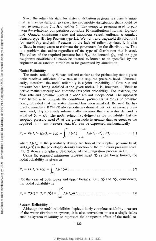
Since the reliability data for water distribution systems are usually mini­mal, it may be difficult to select the probability distribution that should be used in generating Qd, H,,, and/or C. The computer program used to per­form the reliability computation considers 10 distributions [normal, log-nor­mal, Gumbel (minimum value and maximum value), uniform, triangular, Pearson type III, log-Pearson type III, Weibull, and trapezoid distributions] for sensitivity analysis. Because of the lack of reliability data, it is also difficult in many cases to estimate the parameters for the distributions. This is a problem that exists regardless of the type of distribution that is used. The values of the required pressure head Hd, the demand Qd, and the pipe roughness coefficient C could be treated as known to be specified by the engineer or as random variables to be generated by simulation.

Nodal Reliability The nodal reliability R„ was defined earlier as the probability that a given

node receives sufficient flow rate at the required pressure head. Theoreti­cally, therefore, the nodal reliability is a joint probability of flow rate and pressure head being satisfied at the given nodes. It is, however, difficult to derive mathematically and compute this joint probability. For instance, the flow rate and pressure head at a node are not independent. The approach used herein is to compute the conditional probability in terms of pressure head, provided that the water demand has been satisfied. Because the hy­draulic simulator KYPIPE always satisfies demand but not necessarily pres­sure head, this approach automatically assumes that the water demand is satisfied Qs = Qd. The nodal reliability, defined as the probability that the supplied pressure head Hs at the given node is greater than or equal to the required minimum pressure head Hd, can be expressed mathematically

R„ = P(HS > H'd\Qs = Qd) Jo LJo

MH'd)dH'd dHs (1)

where fs(Hs) = the probability density function of the supplied pressure head; and fdi(H'd) = the probability density function of the minimum pressure head. Fig. 2 shows a graphical description of the integration process in Eq. 1.

Using the required minimum pressure head Hd as the lower bound, the nodal reliability is given as

H'd)= t JHi,

R„ = P{HS >H'd)= fs(Hs)dHs (2)

For the case of both lower and upper bounds, i.e., H'd and H"d, considered, the nodal reliability is

/•Hd

Rn = P(Hud >HszH<d)= | fs{Hs)dHs (3) td^HsZHl

d)= . JH'd

System Reliability Although the nodal reliabilities depict a fairly complete reliability measure

of the water distribution system, it is also convenient to use a single index such as system reliability to represent the composite effect of the nodal re-

1123

J. Hydraul. Eng. 1990.116:1119-1137.

Dow

nloa

ded

from

asc

elib

rary

.org

by

UE

M -

Uni

vers

idad

e E

stad

ual D

e M

arin

ga o

n 05

/01/

14. C

opyr

ight

ASC

E. F

or p

erso

nal u

se o

nly;

all

righ

ts r

eser

ved.

fs<Hs)

and

dl d

f (H*) (Demand) dl d

fs(HP and

f d l ^

[*^=}dlK)d<

fs (H8) (Supply)

/

(,<",)

FIG. 2. Steps Involved in Reliability Computation of Nodal Reliability by Eq. 1

liabilities. Such an index is difficult to define because of the dependence of the computed nodal reliabilities. Three heuristic definitions of the system reliability are therefore proposed.

The system reliability Rsm could be defined as the minimum nodal reli­ability in the system

Rsm = min (Rnl), 1,2, (4)

where Rni = the nodal reliability at node i; and / = the number of demand nodes of interest. Another system reliability could be the arithmetic mean Rsa, which is the mean of all nodal reliabilities

2-R.<a — (5)

A third approach could be to define a the system reliability as a weighted average Rsw, which is a weighted mean of all nodal reliabilities weighted by the water supply at the node

1124

J. Hydraul. Eng. 1990.116:1119-1137.

Dow

nloa

ded

from

asc

elib

rary

.org

by

UE

M -

Uni

vers

idad

e E

stad

ual D

e M

arin

ga o

n 05

/01/

14. C

opyr

ight

ASC

E. F

or p

erso

nal u

se o

nly;

all

righ

ts r

eser

ved.

"V -, -

Rs„ = —, (6)

i=\

where Qsi = the mean value of water supply at node ;'. For the purposes of this study, the arithmetic mean and weighted mean are computed in the ex­ample application.

Algorithm The procedure to evaluate the nodal and system reliability of a water dis­

tribution system for hydraulic failure is shown in the flowchart in Fig. 1(b). The algorithm includes the following basic steps:

1. Assign distributions to Qd, Hd and Hd, and/or C. 2. Generate Qd and/or C using Monte Carlo simulation. 3. Compute Hs at all nodes using the hydraulic simulator KYPIPE, assuming

Qd is satisfied (Qs = Qd), 4. Compute nodal and system reliabilities.

A computer program for determining nodal and system reliabilities was developed in FORTRAN V on the CDC Dual Cyber system at the University of Texas. The input data for the model include the physical description of the water distribution system required for KYPIPE, the number of data sets of Qd, Hd, and/or C to be generated, the type of distribution and its pa­rameters for the random variables, etc. Different types of distributions [nor­mal, log-normal, Gumbel (minimum value and maximum value), uniform, triangular, Pearson type III, log-Pearson type III, Weibull, and trapezoid distributions] are coded in the simulation model for examining the sensitivity of the system and nodal reliability to the distributions. Required pressure heads are typically set by health department standards and fire rating asso­ciations. The computer program is written such that the pressure head can be treated as either constant or random, and either with lower bound only or with both lower and upper bounds. It may not be appropriate in many situations to treat the minimum pressure head as a random variable. In order to study the uncertainty of pipe roughness in a particular pipe, the simulation model can also investigate the case in which only a specific pipe of interest has random roughness coefficients, while the pipe roughness coefficients in the remaining pipes are constant. The sensitivity analysis of nodal or system reliability to a particular nodal demand can be done in a similar manner.

EXAMPLE APPLICATION

Example 5A from Wood (1980) as shown in Fig. 3 and Table 1 consists of 17 pipes, and 12 nodes including eight demand nodes is used to dem­onstrate the procedure. For the purposes of illustration, only one demand pattern is considered herein.

1125

J. Hydraul. Eng. 1990.116:1119-1137.

Dow

nloa

ded

from

asc

elib

rary

.org

by

UE

M -

Uni

vers

idad

e E

stad

ual D

e M

arin

ga o

n 05

/01/

14. C

opyr

ight

ASC

E. F

or p

erso

nal u

se o

nly;

all

righ

ts r

eser

ved.

FIG. 3. Example of Pipe Network

In order to compute the nodal and system reliabilities for the water dis­tribution network, the iterative process of random number generation of Qd, Hd and/or C, shown in Fig. 1(a), and hydraulic simulation to compute Hs must be repeated a large number of times. Based upon the results for this application, the computed nodal and system reliabilities can change slightly with the number of iterations. When the number of iterations increase from 200 to 500, the corresponding nodal reliabilities vary about 5-10%; whereas for greater than 500 iterations, the differences in the nodal reliability be­comes insignificant. These conclusions should also be valid for other water distribution systems. For the example used in this study, 500 iterations for random number generation and hydraulic simulation were therefore used. The computer program was run on the mainframe CDC system, Cyber 170/ 750A. Depending on the different input data required, e.g., the type of dis-

TABLE 1. Mean Values of Demands, Required Pressure, and Pipe Roughness Used for Example Network

Node (1)

2 4 5 6 7 9

10 12

Mean demand (cfs) (2)

5.0 4.3 3.7 3.0 5.0 2.0 2.0 2.0

Mean required pressure (ft) (3)

46.9 39.2 38.7 37.3 41.2 48.6 52.2 56.1

Note: Mean pipe roughness is 110 for all pipes.

1126

J. Hydraul. Eng. 1990.116:1119-1137.

Dow

nloa

ded

from

asc

elib

rary

.org

by

UE

M -

Uni

vers

idad

e E

stad

ual D

e M

arin

ga o

n 05

/01/

14. C

opyr

ight

ASC

E. F

or p

erso

nal u

se o

nly;

all

righ

ts r

eser

ved.

TABLE 2. Nodal Reliability Described by Log-Normal Distribution

Node

(D 2 4 5 6 7 9

10 12

Nodal reliability (2)

0.9675 0.9150 0.9300 0.9200 0.9400 0.9675 0.9775 0.9800

tribution used, the required execution time of the program varies from 15.92 to 80.79 CPU seconds for each run.

Table 2 lists nodal reliabilities and Table 3 lists system reliabilities for the case in which Qd, Hd, and C are considered as random variables, with each described by the log-normal distribution. The coefficient of variation for Qd, Hd, and C is assumed to be 0.2. The system reliability using an arithmetic average of the nodal reliabilities and weighted by the nodal flow rate yield similar values for the system reliability. Since the variation of nodal reli­ability is not small nor is the variation in the mean water demand large, similar system reliabilities are to be expected. The nodal demands only dif­fered by a factor of 2.5, whereas in a real system they could differ by over an order of magnitude; with such a difference, the system reliabilities could vary significantly between the two reliability measures.

For cases in which all Qd, Hd, and C are considered as constants, the nodal reliabilities will be equal to one if the required pressure head is sat­isfied or zero if the required pressure head is not satisfied. In the example applications presented in this paper, the mean values of demand, pipe rough­ness, and required pressure head in Table 1 are used, unless they are ex­plicitly specified. Table 4 lists the results of nodal reliabilities for pipe roughnesses of C = 70, 80, and 90 while the demand and the required pres­sure head remain the same. The corresponding system reliability versus the pipe roughness is shown in the curves labeled as "constant C" in Fig. 4, in which the system reliability remains one when the pipe roughness is greater than 90, and drops to zero when C is lower than 70. The other two curves in Fig. 4 are the results obtained by incorporating the uncertainty in the pipe roughness using the normal distribution and a coefficient of variation equal to 0.4. A comparison of the two sets of curves indicates that ignoring un­certainty in the pipe roughness will cause significant overestimation of water

TABLE 3. System Reliabilities for Pipe Roughness, Demand, and Required Pres­sure Head Described by Log-Normal Distribution

Parameter (1)

Rsm

Reliability (2)

0.9497 0.9453 0.9150

1127

J. Hydraul. Eng. 1990.116:1119-1137.

Dow

nloa

ded

from

asc

elib

rary

.org

by

UE

M -

Uni

vers

idad

e E

stad

ual D

e M

arin

ga o

n 05

/01/

14. C

opyr

ight

ASC

E. F

or p

erso

nal u

se o

nly;

all

righ

ts r

eser

ved.

TABLE 4. Nodal Reliability for Constant Pipe Roughness, Demand, and Re­quired Pressure Head

Node (1)

2 4 5 6 7 9

10 12

Pipe roughness 70 (2)

0.00 0.00 0.00 0.00 0.00 0.00 0.00 0.00

Nodal Reliability

Pipe roughness 80 (3)

1.00 0.00 0.00 0.00 0.00 0.00 1.00 1.00

Pipe roughness 90 (4)

1.00 1.00 1.00 1.00 1.00 1.00 1.00 1.00

100 110 120 130

Pipe Roughness C

FIG. 4. System Reliability for Pipe Roughness

1128

J. Hydraul. Eng. 1990.116:1119-1137.

Dow

nloa

ded

from

asc

elib

rary

.org

by

UE

M -

Uni

vers

idad

e E

stad

ual D

e M

arin

ga o

n 05

/01/

14. C

opyr

ight

ASC

E. F

or p

erso

nal u

se o

nly;

all

righ

ts r

eser

ved.

in

Si

4-"

1.0—

0.8 —

0.6 —

0.4 —

0.2 —

0.0

_ ^ — • " — — - - _ _ ,

>§V\JL , A, ' S k f ' ^ r w

-O- Gumbel ^ ^ n -•- Pearson III •X- LogPearson III •+• Normal -D- Log-normal -$- Weibull (skewness=1.5)

I | 1 | I | I | 1

0.0

FIG.

0.2 0.4 0.6 0.8

Coefficient of Variation of C

5. System Reliability for Distributions of Pipe Roughness

1.0

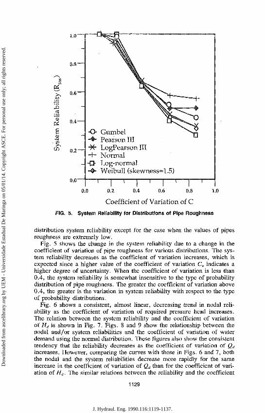
distribution system reliability except for the case when the values of pipes roughness are extremely low.

Fig. 5 shows the change in the system reliability due to a change in the coefficient of variation of pipe roughness for various distributions. The sys­tem reliability decreases as the coefficient of variation increases, which is expected since a higher value of the coefficient of variation C„ indicates a higher degree of uncertainty. When the coefficient of variation is less than 0.4, the system reliability is somewhat insensitive to the type of probability distribution of pipe roughness. The greater the coefficient of variation above 0.4, the greater is the variation in system reliability with respect to the type of probability distributions.

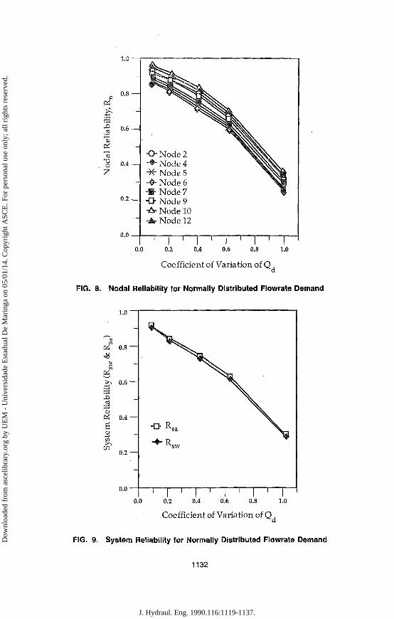
Fig. 6 shows a consistent, almost linear, decreasing trend in nodal reli­ability as the coefficient of variation of required pressure head increases. The relation between the system reliability and the coefficient of variation of Hd is shown in Fig. 7. Figs. 8 and 9 show the relationship between the nodal and/or system reliabilities and the coefficient of variation of water demand using the normal distribution. These figures also show the consistent tendency that the reliability decreases as the coefficient of variation of Qd increases. However, comparing the curves with those in Figs. 6 and 7, both the nodal and the system reliabilities decrease more rapidly for the same increase in the coefficient of variation of Qd than for the coefficient of vari­ation of Hd. The similar relations between the reliability and the coefficient

1129

J. Hydraul. Eng. 1990.116:1119-1137.

Dow

nloa

ded

from

asc

elib

rary

.org

by

UE

M -

Uni

vers

idad

e E

stad

ual D

e M

arin

ga o

n 05

/01/

14. C

opyr

ight

ASC

E. F

or p

erso

nal u

se o

nly;

all

righ

ts r

eser

ved.

i.o • i

0.9 —

0.8 —

S 0.7 — ps5 1^ 0.6 — T3 r ^

& 0.5 — QJ

£ 0 . 4 -

O 0.3 —

0.2 —

0.1 —

^ ^ ^ ^ ^ ^ ^ ^

v — ^ ^ ^ ^ ^ ^ ^ ^ ^ ^ ^ ^ ^ F ^ ^ ^ ^ ^ ^

O Node 2 -*•" Node 4 ~X" Node 5 -$- Node 6 • * Node 7 •O- Node 9 -A- Node 10 ^ r Node 12

1 | , | I | I | I |

0.0 0.2 0.4 0.6 0.8 1.0

Coefficient of Variation of H , d

FIG. 6. Nodal Reliability for Normally Distributed Pressure Head

of variation of pipe roughness are shown in Figs. 10 and 11. As the coef­ficient of variation of C increases above 0.4, the rate of change in reliability is reduced. This can be explained partly because the normal distribution is truncated because of the nonnegativity of values of C, and partly because reliability does become less sensitive to the uncertainty in C when the coef­ficient of variation of C is large. Figs. 12 and 13 show the resulting system reliability for a range of equal coefficients of variation of Qd, Hd, and C. As expected, the reliability decreases as the coefficient increases.

PRACTICAL IMPLICATIONS

The example system presented in this paper is extremely unreliable by standards applied to modern water systems. Real water systems in developed nations have reliabilities on the order of 0.999. When all pipes are in service and there are no emergency (e.g., fire) flows, failure to meet requirements is a rare event. The implication when applying this method to real systems is that the Monte Carlo approach would spend most of its time working on solutions that are reliable. Some heuristic rules may be needed to identify

1130

J. Hydraul. Eng. 1990.116:1119-1137.

Dow

nloa

ded

from

asc

elib

rary

.org

by

UE

M -

Uni

vers

idad

e E

stad

ual D

e M

arin

ga o

n 05

/01/

14. C

opyr

ight

ASC

E. F

or p

erso

nal u

se o

nly;

all

righ

ts r

eser

ved.

t—<

0.0 0.2 0.4 0.6 0.8 1.0

Coefficient of Variation of H , d

FIG. 7. System Reliability for Normally Distributed Pressure Head

Monte Carlo iterations that will obviously meet the constraints without the need to run time-consuming simulations.

Fire flows are rare events in which the demand may be one-to-two orders of magnitude greater than average demand. Such flows do not fit the normal distribution of demand very well. One option to circumvent the shortcoming of the distribution is to include another random variable for fire flow at each low probability of occurrence. Another option is the system where fire flows are not large with respect to average flows.

A primary cause of unreliability is the removal of water lines or pumps from service primarily due to breaks or power outages. The methodology presented in this paper can incorporate removing pipes or pumps from ser­vice due to mechanical failure. A probability of a component being out of service can be included as another random variable in the program.

Water systems and their associated demands are not constant but rather change as utilities grow. The methodology presented in this paper calculates the reliability of a given system at a given time. As pipes or new customers are added to the system, the reliability must be recalculated.

The ultimate goal of this model development will be to incorporate the network reliability procedure into the optimization model by Lansey and Mays

1131

J. Hydraul. Eng. 1990.116:1119-1137.

Dow

nloa

ded

from

asc

elib

rary

.org

by

UE

M -

Uni

vers

idad

e E

stad

ual D

e M

arin

ga o

n 05

/01/

14. C

opyr

ight

ASC

E. F

or p

erso

nal u

se o

nly;

all

righ

ts r

eser

ved.

m 01

13 o

1.0 —

-

0.8 —

0.6 —

-

0.4 —

-

0.2 _

N ^ ^ ^ k

•O Node 2 l l | ^ -•• Node 4 l i ^ y . -X- Node 5 ^ V » -4- Node 6 >H -•r Node 7 |J -O Node 9 •A- Node 10 - ^ Node 12

1 | 1 | I | i | • . | - !

0 .0 0 .2 0.4 0 .6 0.8 1.0

Coefficient of Variation of Q, d

FIG. 8. Nodal Reliability for Normally Distributed Flowrate Demand

"i—|—r 0.2 0.4 0.6 0.8 1.0

Coefficient of Variation of Q

FIG. 9. System Reliability for Normally Distributed Flowrate Demand

1132

J. Hydraul. Eng. 1990.116:1119-1137.

Dow

nloa

ded

from

asc

elib

rary

.org

by

UE

M -

Uni

vers

idad

e E

stad

ual D

e M

arin

ga o

n 05

/01/

14. C

opyr

ight

ASC

E. F

or p

erso

nal u

se o

nly;

all

righ

ts r

eser

ved.

T 1

O

0.8-

0 . 6 -

0.4-

0.2-

0.0-

O Node 2 - • • Node 4 -K- Node 5 -$- Node 6 • * Node 7 -D- Node 9 •AT Node 10

- -A- Node 12

0.0 0.2 0.4 0.6 0.8 1.0

Coefficient of Variat ion of C

FIG. 10. Nodal Reliability for Normally Distributed Pipe Roughness

0.6 0.8 1.0

Coefficient of Variat ion of C

FIG. 11. System Reliability for Normally Distributed Pipe Roughness

1133

J. Hydraul. Eng. 1990.116:1119-1137.

Dow

nloa

ded

from

asc

elib

rary

.org

by

UE

M -

Uni

vers

idad

e E

stad

ual D

e M

arin

ga o

n 05

/01/

14. C

opyr

ight

ASC

E. F

or p

erso

nal u

se o

nly;

all

righ

ts r

eser

ved.

1.0 —

pf 0 . 8 -

M 0 . 6 -01

O 2 " • * -

-

0.2 —

O Node 2 \ J •+ Node 4 •X- Node 5 -$- Node 6 • » Node 7 -D- Node 9 -A- Node 10 - * Node 12

1 "| l " | i ' 1 ' 1 0.0 0.2 0.4 0.6 0.8 1.0

Coefficient of Variation of Q . H ,, and C d d

FIG. 12. Nodal Reliability for Normally Distributed Demand, Pressure Head, and Pipe Roughness

«a

•r- |

Sys

tem

Re

1.0

0.8

0.6

0.4

0.2

0.0

" ° R s a Ife. _̂ -

1

sw ^ ^ * V .

1 ' 1 1_ 1 ' 1 "•" 1 0.0 0.2 0.4 0.6 0.8 1.0

Coefficient of Variation of Q,, H ,, and C d a

FIG. 13. System Reliability for Normally Distributed Demand, Pressure Head, and Pipe Roughness

1134

J. Hydraul. Eng. 1990.116:1119-1137.

Dow

nloa

ded

from

asc

elib

rary

.org

by

UE

M -

Uni

vers

idad

e E

stad

ual D

e M

arin

ga o

n 05

/01/

14. C

opyr

ight

ASC

E. F

or p

erso

nal u

se o

nly;

all

righ

ts r

eser

ved.

(1989) for optimal reliability-based designs. The methodology is based upon an optimal control formulation that couples a hydraulic simulation model with a nonlinear programming solver. Essentially, the hydraulic simulation model implicitly reduces the constraint space of the nonlinear programming problem by solving the continuity and energy equations implicitly each time they need to be evaluated in the nonlinear programming procedure. The non­linear programming problem size is further reduced by using an augmented Lagrangian approach to incorporate the pressure head bounds into the ob­jective function. This particular model WADSOPT (water distribution sys­tem optimization) combines the University of Kentucky KYPIPE model by Wood (1980) for the hydraulic simulation and the generalized reduced gra­dient code GRG2 by Lasdon and Waren (1986) for the nonlinear program­ming optimization. This type of procedure has also been used for the optimal reliability-based design of pumping systems for water distribution systems (Duan and Mays 1990; Duan et al. 1990).

CONCLUSIONS

A methodology has been presented for determining the nodal and system hydraulic reliabilities of water distribution networks. Such a methodology can be used for the assessment of existing systems, the design of new sys­tems, or the expansion of existing systems. The findings from the application presented herein can be summarized as follows:

1. Ignoring uncertainties can cause the overestimation of water distribution system reliability.

2. The coefficient of variation of pipe roughness indicates the degree of un­certainty in the pipe roughness so that the nodal reliability and the system re­liability decrease as the coefficient of variation of pipe roughness increases. This rate of change in the reliability decreases as the value of pipe roughness becomes more uncertain.

3. The degree of significance of the uncertainty in pipe roughness to the re­liability of the water distribution system is dependent on the distribution of pipe roughness used.

4. The nodal and/or system reliability is more sensitive to the uncertainty in water demand than pipe roughness, and, comparatively, the uncertainty in pres­sure head has the least effect on the reliability.

5. The difference in system reliability between the arithmetic mean of nodal reliabilities and the weighted mean of nodal reliabilities is insignificant possibly due to the demand data.

6. The system reliability is not sensitive to the type of distribution of pipe roughness when its coefficient of variation is small.

7. According to many health department rules, all nodes must meet head re­quirements, not just critical ones; therefore, the geometric mean may be the best way to combine nodal reliabilities to assure a system reliability.

8. The methodology can be expanded to incorporate other components, e.g., pumps, valves, tanks, etc., that make up water distribution systems.

ACKNOWLEDGMENTS

The research upon which this paper is based was supported by the National

1135

J. Hydraul. Eng. 1990.116:1119-1137.

Dow

nloa

ded

from

asc

elib

rary

.org

by

UE

M -

Uni

vers

idad

e E

stad

ual D

e M

arin

ga o

n 05

/01/

14. C

opyr

ight

ASC

E. F

or p

erso

nal u

se o

nly;

all

righ

ts r

eser

ved.

Science Foundation Project Assessment of Aging Water Distribution Sys­tems, Grant No. ECE-8511399.

APPENDIX. REFERENCES

Beim, G. K., and Hobbs, B. F. (1988). "Analytical simulation of water system capacity reliability. 2: A markov chain approach and verification of the models." Water Resour. Res., 24(9), 1445-1458.

Billinton, R., and Allan, R. N. (1983). Reliability evaluation of engineering systems: Concepts and techniques. Pitman Books Limited, London, England.

Billinton, R., and Allan, R. N. (1984). Reliability evaluation of power systems. Pit­man Books Limited, London, England.

Coals, A., and Goulter, I. C. (1985). "Approaches to the consideration of reliability in water distribution networks." Proc. 1985 Int. Symp. on Urban Hydrology, Hy­draulic Infrastructure, and Water Quality Control, The University of Kentucky, Lexington, Ky.( 287-295.

Cullinane, M. J. (1989). "Methodologies for the evaluation of water distribution system reliability/availability," thesis presented to the Department of Civil En­gineering, University of Texas, at Austin, Tex., in partial fulfillment of the re­quirements for the degree of Doctor of Philosophy.

Duan, N., and Mays, L. W. (1990). "Reliability analysis of pumping systems." J. Hydr. Engrg., ASCE, 116(2), 230-248.

Duan, N., Mays, L. W., and Lansey, K. E. (1990). "Optimal reliability-based design of pumping and distribution systems." J. Hydr. Engrg., ASCE, 116(2), 249-268.

Henley, E. J., and Kumamoto, H. (1981). Reliability engineering and risk assess­ment. Prentice-Hall, Inc., Englewood Cliffs, N.J.

Hobbs, B. F., and Beim, G. K. (1988). "Analytical simulation of water system capacity reliability. 1: Modified frequency-duration analysis." Water Resour. Res., 24(9), 1431-1444.

Lansey, K. E., and Mays, L. W. (1987). "Optimal design of large scale water dis­tribution systems." Hydraulic Engineering, R. M. Ragan, ed., ASCE, New York, N.Y., 475-480.

Lansey, K. E., and Mays, L. W. (1989). "Optimization model for water distribution system design." J. Hydr. Engrg., ASCE, 115(10), 1401-1418.

Lasdon, L. S., and Waren, A. (1986). GRG2 user's guide. Department of General Business, The University of Texas, Austin, Tex.

Mays, L. W. (1989a). "New methodologies for the reliability-based analysis and design of water distribution systems." Technical Report CRWR 227, Center for Research in Water Resources, Univ. of Texas, Austin, Tex.

Mays, L. W. (1989b). Reliability analysis of water distribution systems. American Society of Civil Engineers, New York, N.Y.

Mays, L. W., and Cullinane, M. J. (1986). "A review and evaluation of reliability concepts for design of water distributions systems." Miscellaneous Paper EL-86-1, U.S. Engineer Waterways Experiment Station, Vicksburg, Miss.

Mays, L. W., Duan, N., and Su, Y. C. (1986). "Modeling reliability in water dis­tribution network design." Proc. Water Forum 1986: World Water Issues in Evo­lution, M. Karamouz, G. R. Baumli, and W. Brick, ASCE, New York, N.Y., 1272-1279.

Quimpo, R. G., and Shamir, U. M. (1987). "Network analysis for water supply reliability determination." Proceedings in hydraulic engineering, R. M. Ragan, ed., ASCE, New York, N.Y., 475-480.

Su, Y. C , et al. (1987). "Reliability-based optimization model for water distribution systems." J. Hydr. Engrg., 114(12), 1539-1556.

Tung, Y. K. (1985). "Evaluation of water distribution network reliability." Proc, ASCE Hydraulics Div. Specialty Conf, Orlando, Fla., 359-364.

Wagner, J. M., Shamir, U., and Marks, D. H. (1986). "Reliability of water distri­bution systems." Report No. 312, Ralph M. Parsons Laboratory, Massachusetts Institute of Technology, Cambridge, Mass.

Wagner, J. M., Shamir, U., and Marks, D. H. (1988a). "Water distribution reli-

1136

J. Hydraul. Eng. 1990.116:1119-1137.

Dow

nloa

ded

from

asc

elib

rary

.org

by

UE

M -

Uni

vers

idad

e E

stad

ual D

e M

arin

ga o

n 05

/01/

14. C

opyr

ight

ASC

E. F

or p

erso

nal u

se o

nly;

all

righ

ts r

eser

ved.

ability: Analytical methods." J. Water Resour. Ping, and Mgmt., ASCE, 114(3), 253-2/5.

Wagner, J. M., Shamir, U., and Marks, D. H. (1988b). "Water distribution reli­ability: Simulation methods." / . Water Resour. Ping, and Mgmt., ASCE, 114(3), 276-294.

Wood, D. J. (1980). "Computer analysis of flow in pipe networks including extended period simulations." Reference material for three-day short course and corre­spondence course, Office of Continuing Education and Extension of the College of Engineering, University of Kentucky, Lexington, Ky.

1137

J. Hydraul. Eng. 1990.116:1119-1137.

Dow

nloa

ded

from

asc

elib

rary

.org

by

UE

M -

Uni

vers

idad

e E

stad

ual D

e M

arin

ga o

n 05

/01/

14. C

opyr

ight

ASC

E. F

or p

erso

nal u

se o

nly;

all

righ

ts r

eser

ved.