MODEL EVALUATION GUIDANCE AND PROTOCOL DOCUMENT

Edited by:

Rex Britter and Michael Schatzmann

COST Action 732

QUALITY ASSURANCE AND IMPROVEMENT OF MICRO-SCALE METEOROLOGICAL MODELS

1 May 2007

Legal notice by the COST Office Neither the COST Office nor any person acting on its behalf is responsible for the use which might be made of the information contained in the present publication. The COST Office is not responsible for the external web sites referred to in the present publication. Contact: Carine Petit Science Officer COST Office Avenue Louise 149 1050 Brussels Belgium Tel: + 32 2 533 38 31 Fax: + 32 2 533 38 90 E-mail: cpetit@cost.esf.org Edited by Rex Britter and Michael Schatzmann

Contributing authors: Alexander Baklanov, Photios Barmpas, John Bartzis, Ekaterina Batchvarova, Kathrin Baumann-Stanzer, Ruwim Berkowicz, Carlos Borrego, Rex Britter, Krzysztof Brzozowski, Jerzy Burzynski, Ana Margarida Costa, Bertrand Carissimo, Reneta Dimitrova, Jörg Franke, David Grawe, Istvan Goricsan, Antti Hellsten, Zbynek Janour, Ari Karppinen, Matthias Ketzel, Jana Krajcovicova, Bernd Leitl, Alberto Martilli, Nicolas Moussiopoulos, Marina Neophytou, Helge Olesen, Chrystalla Papachristodoulou, Matheos Papadakis, Martin Piringer, Silvana di Sabatino, Mats Sandberg, Michael Schatzmann, Heinke Schlünzen, Silvia Trini-Castelli. © COST Office, 2007 No permission to reproduce or utilize the contents of this book by any means is necessary, other than in the case of images, diagrams or other material from other copyright holders. In such cases permission of the copyright holders is required. This book may be cited as: Title of the book and Action Number ISBN: 3-00-018312-4 Distributed by University of Hamburg Meteorological Institute Centre for Marine and Atmospheric Sciences Bundesstraße 55 D – 20146 Hamburg, Germany

3

Contents 1 INTRODUCTION AND CONTEXT............................................................................................ 5 2 SCIENTIFIC EVALUATION....................................................................................................... 8 3 VERIFICATION........................................................................................................................... 11

3.1 VERIFICATION OF MODELS AND THEIR RESULTS .......................................................11 3.2 NON-CFD CODES.......................................................................................................11 3.3 CFD CODES................................................................................................................11

3.3.1 Code verification.......................................................................................................11 3.3.2 Solution verification..................................................................................................11

4 VALIDATION DATA REQUIREMENTS AND AVAILABILITY....................................... 12 4.1 VALIDATION TEST CASES...........................................................................................12 4.2 LABORATORY OR FIELD EXPERIMENTAL DATA.........................................................12 4.3 POTENTIAL VALIDATION DATA SETS........................................................................15

5 MODEL VALIDATION .............................................................................................................. 15 5.1 INTRODUCTION ..........................................................................................................15 5.2 PROCESSING OF THE EXPERIMENTAL DATA...............................................................16 5.3 WHAT VARIABLES TO COMPARE?..............................................................................16 5.4 HOW SHOULD THE VARIABLES BE COMPARED?.........................................................16 5.5 HOW SHOULD THE MODEL BE RUN AND THE RESULTS INTERPRETED? ......................17

5.5.1 Modelling inputs .......................................................................................................17 5.5.2 Setting-up and running of the model ........................................................................17 5.5.3 Post treatment of model outputs ...............................................................................18 5.5.4 Sensitivity analysis (optional)...................................................................................18 5.5.5 Who should run the model and under what conditions? .........................................18

5.6 EXPLORATORY DATA ANALYSIS................................................................................18 5.7 METRICS FOR A MODEL VALIDATION .......................................................................18 5.8 THE BOOT SOFTWARE..............................................................................................19 5.9 QUALITY ACCEPTANCE CRITERIA ..............................................................................19 5.10 A POSSIBLE BASELINE APPROACH TO MODEL VALIDATION .....................................20

6 OPERATIONAL USER EVALUATION................................................................................... 20 6.1 DOCUMENTATION......................................................................................................21 6.2 USER TRAINING AND SUPPORT...................................................................................21 6.3 GRAPHICAL USER INTERFACES (GUIS) AND INPUT DATA FORMATS .........................21 6.4 USER RESPONSIBILITIES.............................................................................................22

7 REFERENCES.............................................................................................................................. 23

APPENDIX 1 PITFALLS AND RESTRICTIONS ................................................................... 25 A. GENERAL ADVICE .................................................................................................................25 B. VALIDATION .................................................................................................................25 C. MODELLING .................................................................................................................25 D. WIND TUNNEL DATA .................................................................................................................26 E. FIELD DATA .................................................................................................................26

4

5

1 Introduction and Context

Models of whatever type are only of use if their quality (fitness-for-purpose) has been quantified, documented, and communicated to potential users. This process, called Model Evaluation, can enhance our confidence in the use of models developed for environmental and other problems. It may not be appropriate to talk of a valid model, but only of a model that has agreed upon regions of applicability and quantified levels of performance (accuracy) when tested upon certain specific and appropriate data sets.

The main objective of COST Action 732 is the determination and improvement of model quality for the application of micro-scale meteorological models to the prediction of flow and dispersion (dispersion = transport plus diffusion) processes in urban or industrial environments. The approach adopted in COST 732 is to produce three documents that are intended to assist model developers and users in the evaluation of mathematical models:

• A BACKGROUND AND JUSTIFICATION DOCUMENT TO SUPPORT THE MODEL EVALUATION GUIDANCE AND PROTOCOL

• A BEST PRACTICE GUIDELINE FOR THE CFD SIMULATION OF FLOWS IN THE URBAN ENVIRONMENT

and this document

• THE MODEL EVALUATION GUIDANCE AND PROTOCOL DOCUMENT

This third document is a stand alone document to assist the setting up and executing of a model evaluation exercise.

All three documents are based on a fourth COST 732 document, the proceedings from a workshop on

• ‘QUALITY ASSURANCE OF MICROSCALE METEOROLOGICAL MODELS’

which was jointly organized by COST 732 and the European Science Foundation and was held in Hamburg in July 2005 (Schatzmann and Britter, 2005). The documents are available from the COST 732 homepage under http://www.mi.uni-hamburg.de/Home.484.0.html.

When determining model quality (fitness-for-purpose), it is obviously essential to consider and specify what the purpose of the model is. For example models with a similar scientific basis may be required for quite different purposes such as:

• A model for planning or regulatory purposes may need to be run several thousands of times

• A model for emergency response may need real-time predictions or access to pre-calculated real-time output

• A model for post-accident investigation or air quality hot spot analysis could be very complex with less concern for computational cost or resource requirement

The title of COST 732 provides a good starting point to produce a statement as to the purpose of the models under consideration; that is “Microscale meteorological models”. COST 732 has interpreted this as models for the prediction of the flow

6

and/or the dispersion of pollutants within and near the urban canopy or industrial landscape. To proceed further requires broad specification of the range of time and space scales of interest and whether the application is typically steady or unsteady. Computational Fluid Dynamics (CFD) models are thought to be an appropriate tool for this application and their evaluation is central to COST 732. However the application of simpler models to these problems is of direct interest to many participants in COST 732 and our methodology must allow for the evaluation of a range of model types. Our approach has been to develop a methodology that can be used for CFD models and can also be modified to accept simpler models.

The micro-scale meteorological models of interest are (ordered by computing costs):

• CFD (LES)

• CFD (RANS, URANS)

• Semi-Empirical models such as

• Surface roughness based models

• Porosity type models

• Diagnostic models (which ensure mass consistency only)

• Analytical models

The dispersion models of interest are:

• CFD (LES)

• CFD (RANS, URANS)

• Semi-Empirical and Empirical models such as

• Lagrangian models

• Simple Urban Dispersion Correlation (SUDC)

• Gradient transport ( K-theory) models

• Gaussian plume or puff type models

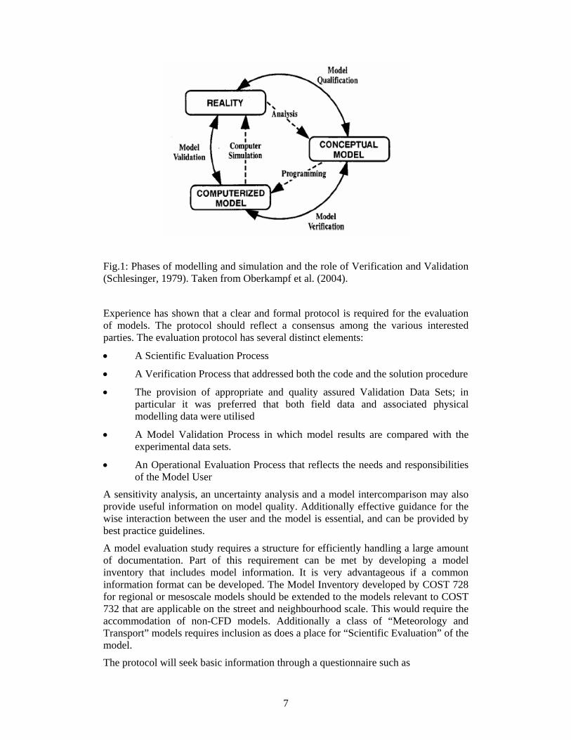
Oberkampf et al. (2004) adopts the basic methodology of model evaluation from the AIAA guideline (AIAA, 1998). Their view of the role of model evaluation in the different phases of modelling is shown in Figure 1 (Schlesinger, 1979). Analysis of reality produces a conceptual model that comprises all the equations that are necessary to describe (at some specified level of detail) the problem, including initial and boundary conditions.

The appropriateness of the analysis is assessed through qualification though we prefer the term scientific evaluation. The implementation of these equations into an operational computer program is called the computerised model. From Figure 1 it is clear that verification deals with the relationship between the conceptual and the computerised model. Validation on the other hand deals with the relationship between the computerised model and experimental measurements.

7

Fig.1: Phases of modelling and simulation and the role of Verification and Validation (Schlesinger, 1979). Taken from Oberkampf et al. (2004).

Experience has shown that a clear and formal protocol is required for the evaluation of models. The protocol should reflect a consensus among the various interested parties. The evaluation protocol has several distinct elements:

• A Scientific Evaluation Process

• A Verification Process that addressed both the code and the solution procedure

• The provision of appropriate and quality assured Validation Data Sets; in particular it was preferred that both field data and associated physical modelling data were utilised

• A Model Validation Process in which model results are compared with the experimental data sets.

• An Operational Evaluation Process that reflects the needs and responsibilities of the Model User

A sensitivity analysis, an uncertainty analysis and a model intercomparison may also provide useful information on model quality. Additionally effective guidance for the wise interaction between the user and the model is essential, and can be provided by best practice guidelines.

A model evaluation study requires a structure for efficiently handling a large amount of documentation. Part of this requirement can be met by developing a model inventory that includes model information. It is very advantageous if a common information format can be developed. The Model Inventory developed by COST 728 for regional or mesoscale models should be extended to the models relevant to COST 732 that are applicable on the street and neighbourhood scale. This would require the accommodation of non-CFD models. Additionally a class of “Meteorology and Transport” models requires inclusion as does a place for “Scientific Evaluation” of the model.

The protocol will seek basic information through a questionnaire such as

8

Protocol: Basic Information Questionnaire

Information required here should include:

• Name and contact information of person providing information

• Name, version number and release date of the model

• A brief description of the intended use of the model

• Model type

• Inputs required

• Quantities predicted

• Route of model into evaluation project; developer, supplier, user

• Model history or provenance including model ancestors

• Quality assurance standards adopted in model and software development

• Status of model with respect to other models i.e. is the model self-contained or not

• Current model usage; type of user/distribution of model/number of users

• Hardware and software requirements

• Model availability and costs

This information need not be evaluated. The information obtained here should be entered in a documentation system; the preferred option is to use the Model Inventory developed under COST 728 that has now been modified to accept COST 732 requirements.

2 Scientific Evaluation

A model evaluation requires a Scientific Evaluation whose primary objectives are:

• to ensure that all important phenomena within the models’ ranges of application are included

• to ensure that the mathematical modelling of these phenomena and the associated simplifications and parameterizations are well justified in terms of science and model practicality and

• that the limits of model applicability are clear and explicit

• to ensure that the user or prospective user is able to judge the suitability or not of the model for their specific purpose

The Scientific Evaluation requires a detailed description of the model physics and chemistry and, most importantly, an assessment or judgement as to the appropriateness of this scientific content for the purpose of the model. This “judgement” must inevitably be a consensus of those experts in the field. One point of COST 732 is to produce that consensus from experts across Europe in an objective manner.

Three recent European model evaluation projects provide useful background and experience.

9

In the SMEDIS Project (Daish et al., 2000) funded by the European Union a methodology for the Scientific Evaluation of the dense gas dispersion models was developed. It was mainly based on a questionnaire to be completed by each modeller, covering all the evaluation aspects. The scientific evaluation questions refer to issues such as the problems addressed by the model (that is, the purpose of the model) and the physical and chemical processes modelled.

The recent guideline of the VDI (the German Association of Engineers) addresses the issue of Scientific Evaluation mainly in terms of the input data, the domain and grid description, the general equation system and its simplifications, the various parameterisations that are important in micro-scale modelling, the turbulence closure, the boundary and initial conditions and the output data.

For atmospheric flows at the street or neighbourhood scale it is worth mentioning also the recommendations as to the use of CFD (RANS type) in the area of wind engineering performed under COST C14 (Franke et al., 2004). This paper addresses the problems of the basic equations, the turbulence models, the computational domain and the numerical approaches.

The use of a common questionnaire, agreed upon by, for example, informed European stakeholders, but completed by model developers and users may be the least resource demanding approach.

The questionnaire also allows scope for the developer or user to provide information on the intended applications of the model and any specific limitations on the use of the model.

Integral to the scientific evaluation is the provision of a brief model description. This description should allow a user or evaluator to obtain a quick overview of the model including the model capabilities and limitations. An additional important consideration is that the Scientific Evaluation is undertaken objectively. It can be argued that this requires that the Scientific Evaluation should be undertaken independently of the model developer or user. In practice this can be quite difficult because the developer or the users are often in the best position to provide a sound understanding of the model attributes and limitations. The provision of one or more signatures accepting responsibility for the accuracy of the completed questionnaire should be adequate to maintain objectivity.

For the Scientific Evaluation to most effectively meet its purpose it is preferable that both CFD and non-CFD models are addressed in a uniform manner wherever possible.

Protocol: Scientific Evaluation

The Scientific Evaluation is to be based on a questionnaire. The approach will be to:

1. Specify clearly the model purpose(s) e.g. prediction of the flow and/or dispersion of pollutants within an urban area. The required spatial and temporal resolution and accuracy should be stated.

2. Produce a consensus of what “science” is required for this model and its applications

3. Determine whether the “science” is present in an adequate form in the models being evaluated

4. Provide clear documentation on the above.

10

Those evaluating models must state the model purpose(s) as in point 1 above. The items below provide a guide as to what might be included within points 2 and 3. The information obtained here should be entered in a documentation system; the preferred option is to use the Model Inventory developed under COST 728 that has now been modified to accept COST 732 requirements. This would satisfy point 4.

CFD and non-CFD models; flow and/or dispersion

Model information required here could include the:

• brief model description

• equations solved (including the fundamental equation system and any simplifications or approximations introduced)

• spatial (micro, meso, macro) and temporal ( minutes, hours, days, years) scale

• turbulence parameterisation

• computational domain

• grid design and resolution (CFD models only)

• numerical solution approach

• near surface treatment e.g. wall functions

• boundary conditions

• initial conditions

• input and output data

• implicit or explicit averaging time for output

• specification of the source

• applicability or not to specific scenarios such as

1. time varying input

2. non-neutral atmosphere

3. complex terrain

4. buildings (essential)

5. calm or light wind conditions

6. heat and mass transfer with underlying surface and other surfaces

7. chemistry

8. positively or negatively buoyant pollutants

9. aerosols and particulate matter

10. concentration fluctuations (including probability density functions)

11. phase changes

12. wet and dry deposition

13. radioactivity

14. solar radiation

11

15. treatment of trees and parks

16. treatment of surface roughness ( general and on building surfaces)

17. traffic induced turbulence

It must be stressed that the “applicability” items here only indicate that the model has attempted to address these issues. The Scientific Evaluation should comment on the appropriateness or not of the science used in the model to address these issues.

3 Verification

3.1 Verification of models and their results

Verification is an important part of the model evaluation. There are two aspects of verification; the verification of the models also known as code verification and the verification of the solution procedure also known as solution verification. Code verification is used to demonstrate that the computational model is consistent with the conceptual model. Solution verification is used to estimate the numerical error in a given numerical solution. Both aspects are present in CFD and non-CFD models.

3.2 Non-CFD codes

The code and solution verification of non-CFD models is relatively straightforward in the sense that their size and complexity is normally limited and line-by-line interrogation is possible. In practice however, often the verification is not comprehensive and relies on the calculation of a number of known, possibly analytical or hand-calculated solutions. Another technique is to check for internal consistency, such as mass and/or mass flux balances or performing the same calculation in two or more different ways. The behaviour of the model in certain limiting conditions can also be used.

If resources permit within COST 732 an investigation of the formal application of the techniques in 3.3 to non-CFD codes should be undertaken.

3.3 CFD codes

3.3.1 Code verification

Code verification is an issue for which the code developer is responsible.

The following steps should be taken by the code developers:

• Provision of information about the general software quality assurance of the code.

• Provision of information about the strategies for code verification.

• Ideally a demonstration that those modules of the code which are activated for the prediction of the flow and pollutant dispersion are consistent with the conceptual model, using the observed order of accuracy test described in the Background document.

Within the COST Action 732 the method of manufactured solutions, which is already used in aeronautics, will be further tested and developed to be applied to microscale meteorological models.

3.3.2 Solution verification

The following steps should be taken when performing validation simulations:

12

• Reduction of the error from incomplete iterative convergence to a negligible magnitude by monitoring the target variables as function of the iteration number.

• Repeating the simulation on at least two more grids with systematic coarsening or refinement.

• Estimating the error band of the computed target variables with methods based on generalised Richardson extrapolation.

Within the COST Action 732 different methods for the estimation of the discretisation error will be tested and compared to find the most appropriate method in the context of the validation of microscale meteorological models for urban dispersion problems

Protocol: Model Verification

The Model Verification will (initially) only request that the code developers or users provide information about the strategies that have been used to ensure satisfactory model verification. This does not necessarily mean that there are no errors, only that formal and documented attempts have been made to locate ay errors.

COST 732 will develop, test and provide some simple and practical guidelines for code and solution verification. The COST 732 Best Practice Guideline (COST 732, 2006B) is an example of this.

4 Validation Data Requirements and Availability

4.1 Validation test cases

A requirement of the model evaluation procedure will be several sets or test cases of observational data with which the simulated data can be compared. Each test case must be easily accessible and come with complete documentation. Generally the test cases should range from the simple to the complex; such as from a single block in a wind tunnel to a single building in the field to a section of a real urban environment.

However it was decided in COST 732 that there was more interest in undertaking model evaluations at the more complex end of this range in order to provide results that would be immediately useful. It has been assumed that the models under discussion have already undergone a basic test phase (model evaluation) with single cubes etc. obtained from physical modelling in a wind tunnel as suggested and provided for in the German VDI Guideline on Evaluation of prognostic micro-scale wind field models for flow around buildings and obstacles (VDI, 2005) or similar. This VDI Guideline is available at modest cost.

COST 732 has argued that we restrict ourselves to real urban and provide only urban validation data. This implies the need for a close collaboration of experts in the fields of observational techniques and modelling. A number of issues have to be taken into account: The quality (fitness-for-purpose) of the test data in terms of accuracy and precision, as well as their spatial and temporal representativeness significantly affect the outcome of the model validation procedure. It must be stated strongly that the results of model validation are as good or as uncertain as the observational data are.

4.2 Laboratory or Field experimental data

The laboratory experiments in wind tunnels and water flumes are ideal in that there is nearly complete control over the experiment. The VDI, 2005 Guideline is based solely

13

on laboratory experiments and these were mainly simple arrangements of one or, in one case, several buildings. This was thought appropriate for the specific objectives of the VDI Guideline.

There is some concern that the evaluation of model quality based solely on physical modelling is an unwise practice and that the use of full scale field experiments and data is an essential part of the evaluation process. This stems from two principal concerns:

• Some aspects of the problem may be extremely difficult or impossible to be physically modelled in a wind tunnel or water flume. This is a particular difficulty when there is need to model several physical phenomena simultaneously. A short list of examples where difficulty exists would include:

1. non-neutral atmospheric stability

2. thermal effects due to heating or cooling of building surfaces; both for aerodynamically smooth and rough surfaces

3. chemical reactions

4. deposition and resuspension

• Physical modelling is based on skilled judgement as to what the important or dominant physical processes are, and this judgement may be wrong or not lead to a definitive solution.

There are two broad types of field data. There is extensive monitoring and associated data sets from permanent field stations both for meteorological and air quality concerns and this is available for model evaluation purposes. Additionally there have been many field experiment campaigns (though until recently these were not at the city or smaller scales) to obtain data under controlled conditions and these are also generally available for evaluation purposes. The former and more extensive sets of field data do not always have corresponding physical modelling equivalents.

Of course field experiments have their own difficulties and limitations; cost and resource provision not being the least. The wise approach, if resources permit, is to use a combined data set comprising laboratory and field experiments, both used within the regions of applicability of each approach. Within COST 732 it was decided that it was preferable to provide data that originated from a combination of field and wind tunnel experiments. If there was inadequate data availability then this may need reconsideration.

The accuracy or reliability of field data cannot easily be quantified based on field data alone. It is not just the accuracy of the instrumentation used for field measurements which defines the reliability of data compiled from field measurements. In addition, the repeatability of field measurements for similar boundary conditions as well as the spatial representativeness of individual measurement locations with respect to a particular flow and dispersion problem must be evaluated and quantified with respect to the measured quantities before corresponding data can be used safely for model validation purposes.

Schatzmann and Leitl (2002) give an impression how severe that not yet widely recognised problem really is. They analysed data presented in form of half-hourly averages from an urban monitoring station for a full year. The large number of data points allowed carrying out a statistical analysis. After some filtering and removal of

14

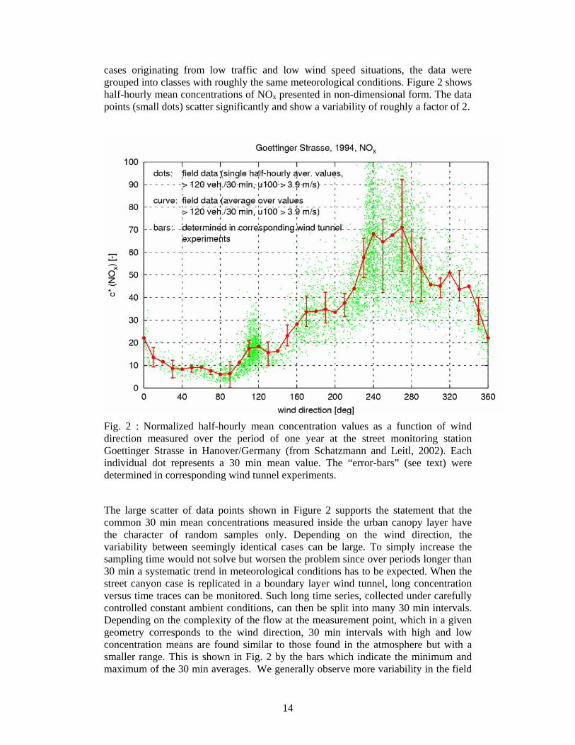
cases originating from low traffic and low wind speed situations, the data were grouped into classes with roughly the same meteorological conditions. Figure 2 shows half-hourly mean concentrations of NOx presented in non-dimensional form. The data points (small dots) scatter significantly and show a variability of roughly a factor of 2.

Fig. 2 : Normalized half-hourly mean concentration values as a function of wind direction measured over the period of one year at the street monitoring station Goettinger Strasse in Hanover/Germany (from Schatzmann and Leitl, 2002). Each individual dot represents a 30 min mean value. The “error-bars” (see text) were determined in corresponding wind tunnel experiments.

The large scatter of data points shown in Figure 2 supports the statement that the common 30 min mean concentrations measured inside the urban canopy layer have the character of random samples only. Depending on the wind direction, the variability between seemingly identical cases can be large. To simply increase the sampling time would not solve but worsen the problem since over periods longer than 30 min a systematic trend in meteorological conditions has to be expected. When the street canyon case is replicated in a boundary layer wind tunnel, long concentration versus time traces can be monitored. Such long time series, collected under carefully controlled constant ambient conditions, can then be split into many 30 min intervals. Depending on the complexity of the flow at the measurement point, which in a given geometry corresponds to the wind direction, 30 min intervals with high and low concentration means are found similar to those found in the atmosphere but with a smaller range. This is shown in Fig. 2 by the bars which indicate the minimum and maximum of the 30 min averages. We generally observe more variability in the field

15

than in the wind tunnel even after other perturbing influences have been considered (such as non-local concentration contributions, variations in the emission rates for any particular traffic count etc). They result from the fact that clouds of pollutants are subject to low frequency disturbances in the atmospheric boundary layer which have time scales that are not small compared to the averaging time. These may not be present or not resolved in the wind tunnel. This is why we are using wind tunnel and field measurements in our evaluation process.

4.3 Potential Validation Data Sets

Following the strict data evaluation concept developed above, only a very limited set of validation data is currently available for testing and validation of 'state-of-the-art' microscale flow and dispersion models. Combined field and laboratory data are available from the MUST experiment (Biltoft, 2001, Harms et al, 2005, Bezpalcova, 2007), the VALIUM study (Schatzmann et al., 2006), the DAPPLE project (Arnold et al 2004) as well as from the BUBBLE project (Rotach et al., 2005) and the Joint Urban 2003 experiment (Allwine, 2004, Leitl et al., 2005). The data sets cover a wide range of geometrical complexity, ranging from a rather simple array of containers to the in-homogeneously structured roughness of the central business district in a modern city. Whereas the field data mainly focus on point-wise, local flow and dispersion measurements the corresponding laboratory data generated in boundary layer wind tunnels provide quasi-stationary flow and dispersion fields (MUST, VALIUM, JU2003) and instantaneous flow and dispersion data for well-defined boundary conditions. Tables 6.1 and 6.2 in Britter and Schatzmann (2007) document the availability of information, not distinguishing between information from wind tunnel experiments and field tests. Currently, the table is based mainly on a literature survey. The content will be updated after approaching the originators of different data directly.

It is intended to homogenize the existing field and laboratory data in order to compile consistent validation data sets. Upon approval of the authors of particular data selected results of corresponding field and laboratory experiments will be merged to form validation data sets as complete as possible, together with all necessary information (modelling inputs) to carry model validation.

Relevant data sets will be peer reviewed and made available for model evaluation purposes.

Protocol: Provision of test case data

COST 732 will provide a peer reviewed urban flow and dispersion data set to initiate a model evaluation study; Working Group 2 has provided this for the MUST experiment in the laboratory.

Further data sets will follow.

5 Model Validation

5.1 Introduction

Validation is the comparison of model predictions with experimental observations (or possibly with the results from more complex models that have themselves undergone formal model evaluation). It is important that there is consensus amongst the scientific and wider community as to the appropriateness of the validation process. In order to

16

conduct a validation, one will have to decide for which purpose the model results should later be used and thus to decide the variable(s) whose prediction is the most important. In other words the validation objectives have to be determined. There are many other questions to ask and answer in setting up a validation study.

5.2 Processing of the experimental data

The experimental data to be used in the validation must be subjected to the following:

• an initial and global evaluation to become familiar with the data and determine their attributes and problems

• determining whether the data are of homogeneous quality or whether some data are of poorer quality than other data

• processing of laboratory data; should the validation study be at laboratory scale or after the data have been scaled up

• treatment of zeros or relatively small data; this is a somewhat critical area so it has been developed further below. In many atmospheric boundary layer experiments there are many very small observed concentrations or wind speeds. The way such data are handled may have a decisive influence on quantitative performance metrics. Experience has shown that this is often a major concern in a model validation study and can be subject to somewhat arbitrary decisions. If the ratio of a predicted to measured concentration is used as a comparator then difficulties will arise and the overall validation metric can be dominated by the smallest concentrations that are being compared. Caution should be paid to this problem. A possible workaround is to impose a filter so that the ratio is considered unity when both predicted and measured concentrations are below a certain threshold. The choice of this threshold is often a sensitive issue. Knowledge of the uncertainty of the experimental data can be used as a guide in determining what data should be discarded or assumed to be of lower quality.

• The use of raw or manipulated (e.g. using volume averaged) experimental data.

• Stochastic variability of velocity and concentration measurements; stratification of field experimental data into similar groups of data

5.3 What variables to compare?

These might be put into a hierarchy of:

• Those directly relevant to the model purpose such as the concentration or the velocity (taken over a specified averaging time).

• Those variables that are intermediaries in determining the variables which are directly relevant to the model purpose.

• Those that are neither of the above but are a useful diagnostic of the performance of the model such as the turbulence intensity.

5.4 How should the variables be compared?

Should the experimental data and model results be compared:

• when paired in space or time, or only in space, or only in time

17

• on a point-wise basis or a footprint basis

• with greater weight be given to agreement of, for example, the larger concentrations rather than the smaller, near zero ones,

• in a way that weights false positives and false negatives differently

• as a difference between the variables or as the ratio of the variables.

The answer will depend principally on the intended purpose of the model.

5.5 How should the model be run and the results interpreted?

The model predictions will be based on the inputs to the modelling, the setting up and running of the model and any manipulation of the model outputs thought necessary. The points made below may seem relatively straightforward if a particular model is being evaluated against a particular data set. However, preparation of input data is often far from trivial. There may be many options for choice and processing of measured data when model input is being prepared. Further difficulties arise and need to be overcome when considering the intercomparison of several models when evaluated against a particular experimental dataset. The models may have different input requirements, different procedures for setting up and running the model and require different treatments of the model outputs. These will need to be reconciled in an equitable way for all models. This issue is of less concern when working with well controlled and extensively measured laboratory data than when using field experimental data. In the latter case there will be little control over the experiment and restricted availability of meteorological and other data. The most appropriate way to work with field data is a subject of much debate within and outside Europe.

5.5.1 Modelling inputs

The inputs required for the model will require specification based on the experiment to be modelled. These would include:

• Terrain, buildings, obstacles either precisely or in some surrogate form such as land use or surface roughness lengths etc.

• Meteorology at whatever level of detail is required for the model. These may be specified based on a particular averaging time.

• Boundary conditions or parameterizations of thermal or mass transfer processes as appropriate.

5.5.2 Setting-up and running of the model

This will depend on the type of model under evaluation but for CFD models would include:

• Deciding on level of detail to be used for the modelling

• Computational domain

• Gridding/meshing techniques

• Choice of turbulence model if a choice is available

• Numerical schemes

• Use of wall functions

• Allowed run time on allowed computer type

18

• The handling of the “averaging time”

5.5.3 Post treatment of model outputs

The outputs may need to be post treated into the same format as that for the raw or manipulated experimental data prior to the comparison of model prediction and experimental data.

5.5.4 Sensitivity analysis (optional)

In order to quantify uncertainties in model outputs in relation to the comparison with observations it is useful to perform a sensitivity analysis, in the form of an ensemble of simulations with slightly varying input parameters.

5.5.5 Who should run the model and under what conditions?

A decision must be made as to whether the model should be run by someone familiar with the model and possibly a proponent of the model or whether it should be run by a neutral party. Typically the realistic option is to have someone familiar with the model running it.

A second decision is to decide whether the model runs should be done blind or whether those running the models should have access to some or all of the experimental data. Typical practice is to use both approaches.

5.6 Exploratory data analysis

It is recommended to perform some exploratory data analysis, where modelled and observed data are plotted in various ways. Such exploratory data analyses are well suited to highlight notable features in data and reveal shortcomings of models.

Commonly used types of plots are:

• Scatter plots

• Quantile-quantile plots

• Residual analysis through residual plots (box plots and scatter plots).

5.7 Metrics for a Model Validation

After a paired set of experimental data and model predictions have been obtained, one or more methods of comparison must be selected and quantified. There are several standard metrics of which the correlation coefficient is the most obvious. Some other frequently used examples are:

FAC2 = Fraction of predictions within a factor of two of the observations.

FB (Fractional Bias) = [ ])CC(5.0)CC( popo +−

NMSE (Normalized Mean Square Error) = po2

po CC)CC( −

MG (Geometric Mean) = ))C/Cln((exp)ClnCln(exp popo =−

VG (Geometric Variance) = [ ] [ ]2po

2po ))C/C(ln(exp)ClnC(lnexp =−

Figure of Merit (FoM) is defined as the ratio of the area marked by the intersection of the predicted and observed concentrations or dosages within a prescribed contour, divided by the union of the two areas

19

Measure of Effectiveness (MoE) assigns different weights to false positives and false negatives.

Hit Rate is another metric that has recently been found useful for velocity models. The German VDI Guideline on prognostic meso-scale wind field models sets requirements in terms of this metric (VDI 2005). To evaluate the model performance, normalized values are compared, with the wind speed used for normalisation. From the normalised model results Pi and normalised comparison data Oi a hit rate q is calculated from the equation below, which specifies the fraction of model results that differ within an allowed range D from the comparison data. D accounts for the relative uncertainty of the comparison data. Only those differences are counted that are above a threshold value W, which describes the repeatability of the comparison data.

⎪⎩

⎪⎨

⎧≤−≤

−=== ∑

=else0

WOPorDO

OPfor1

NwithNn1

nNq ii

i

ii

i

n

1ii

5.8 The BOOT software

A tool that can be useful is the free BOOT software (http://www.harmo.org/kit/BOOT_details.asp). BOOT is a tool designed for statistical performance evaluation, and developed by Chang and Hanna. It is accompanied by a comprehensive, User's Guide (Chang and Hanna, 2005). Besides detailed technical description of performance measures and the use of the software, the User's Guide also provides a discussion of model evaluation objectives and exploratory data analysis. The BOOT package is flexible and general in nature. It seems wise to use free, verified and common software for the data analysis. A recommended tool should be open source and, preferably, usable on different systems, for example Linux

The BOOT package is capable of computing performance measures such as the Fractional Bias (FB), the Normalised Mean Square Error (NMSE), the Geometric Mean Bias (MG), the Geometric Variance (VG), the fraction within a factor of 2 (FAC2), the Measure of Effectiveness (MOE), as well as several others. (FB and MOE are in fact closely related.) BOOT allows FB and MG to be separated into over-predicting and under-predicting components. Bootstrap re-sampling is used to estimate the confidence limits of a performance measure - hence the name BOOT of the package. BOOT is distributed as part of the Model Validation Kit for point source dispersion, and is available at www.harmo.org/kit.

5.9 Quality acceptance criteria

The validation exercise will provide qualitative and quantitative views of the model quality. However this does not address whether or not the quality is acceptable. This is not possible without a clear statement of the purpose of the model and that purpose is converted into limit values for one, more, or all the metrics that are chosen to be relevant. This step must be performed early in any model evaluation process to “ground” the evaluation appropriately. One useful step that can be made is to establish, with experience, values of the metrics that are typical of particular model types when applied to specific problems. In a sense, these metrics and their limit values are a quantitative statement concerning the much-used, but rarely defined concept of the “state-of-the-art”. As examples some opinions are expressed here:

20

• For the maximum concentration on an arc, the acceptable relative mean bias is + or – 50 % and the acceptable relative scatter is factor of two for research grade experiments with source well-known and on-site meteorology. This is a very general statement. More precise statements can be formulated when specific test cases are considered.

• For comparisons with wind tunnel data the German VDI Guideline on wind field models (VDI, 2005) requires a certain hit rate for a number of specific test cases. For example, for wind components at specific points behind a building, the Guideline requires a hit rate of q > 66 % with an allowed deviation D=0.25.

• Other typical values are given by Chang & Hanna (2004)

5.10 A possible Baseline approach to Model Validation

It may be useful to outline a possible baseline approach to a Model Validation. This could proceed with:

• decide to allow those running the models to have access to the experimental results or not ( that is non-blind / blind simulations )

• select the mean velocity and mean concentration ( based on certain temporal and spatial scales) for comparison

• look at the streamline pattern and the concentration pattern to provide a qualitative view of the model quality

• for a quantitative evaluation of the model quality compare the experimental and model data “paired in space and time” and as “arc maxima”. The complexity of the flow may make the latter choice less feasible where local maxima could be everywhere

• use the metrics of FAC 2 (for its transparency) and FB/NMSE (for information on bias and variance). The FB/NMSE weights the higher magnitudes at the expense of the smaller

• for the comparison of mean concentrations the SMEDIS study found that for CFD models applied to scenarios including obstacles such as buildings FAC2 = 0.54 for all data paired in space and time , and 0.89 when using only arc maxima (Carissimo et al., 2001). These would seem to be realistic goals for a validation study to work with.

Protocol: Model Validation

Initially use the Baseline approach to Model Validation outlined in Section 5.10 above.

Use the structure of this chapter to develop future protocols as necessary

6 Operational User Evaluation

This section considers the interests and expectations of the user of a model, whether they are provided by the model developer or vendor (and whether they are adequate) and the experiences of the user with the model. Two general types of user can be discerned; the user working within the research community and actively involved in model development and the user involved in regulatory or consulting activities

21

probably using commercial models or non-commercial but widely distributed models (such as those available from the US Environmental Protection Agency or European National research organisations). This aspect of Model Evaluation includes:

6.1 Documentation

The documentation should be in the form of a User Manual (including a short description of the model) and a Technical Reference Manual (including a more detailed description of the model). It should include:

• Detailed documentation of the physical processes and numerical methods as well as approximations and parameterizations used in the model.

• Comprehensive and well documented evaluation activities.

• The model documentation has to identify shortcomings and restrictions of the model.

• Many models provide tables to assist the user in parameter selection.

• Guidance on mesh generation.

6.2 User training and support

Sufficient training and education of the user by the software developer or provider is desirable. The possibilities of user errors (e.g. in input and definition of the model run) increase with increasing model complexity. User training and support may be necessary in order to minimize this effect. It is expected that this will be available for commercially supplied models. It may include:

• User friendly, well documented, model installation procedure including test case files

• Web pages providing on-line manuals, updates, courses for users, frequently asked questions (FAQs), on-line forums

• Telephone/email support Many commercial code developers have a good policy of differentiated user approach, offering packages of different services such as training, technical support, consulting and university programs. They also organize meetings, workshops and conferences where users can present results of their numerical simulations and discuss different model applications. This approach produces useful feed-back that creates opportunities for further model development.

There is also highly respected and widely accessible open source software developed by academia or other agencies. Some agencies (such as the US EPA) provide a level of support and training for their models. Additionally self-help user groups often form around particular models or modelling activities. These are pragmatic and effective approaches to providing user support and training to the modelling community. For research grade models the user community is often smaller and well-versed in the appropriate use of the models.

6.3 Graphical user interfaces (GUIs) and input data formats

The user interface to the model is also an important consideration. A user-friendly GUI with plausibility checks of the model input help to decrease inconsistencies in the model set-up.

22

A model developer should keep in mind that the user may use different databases of input data and may need to create their own special data pre-processors. Therefore, a comprehensive detailed description of all input data files needs to be provided to the user, together with example files.

6.4 User responsibilities

As Oberkampf et al. (2004) points out, it is impossible for the model developer to cover all possible combinations of physical, boundary and geometrical conditions during the evaluation of the model because of the extremely wide range of possible applications. Furthermore, the software is ported to a wide variety of computer platforms under different operating systems and must be verified for a range of compiler options. This requires a large portion of the responsibility for evaluation to be placed on the model developer but also the user take an active part in order to achieve sound application of the model in a particular situation.

The extensive documentation is essential to enable the user to decide whether the model is the proper tool for a specific application and to assess its strength and weaknesses. Commercial models sold as “black boxes” should not be used for regulatory purposes at all, if an extensive documentation is not provided. On the other hand, if a user decides to modify the codes provided in case of freely accessible models, they must be aware that it may lead to invalidation of any prior model evaluation results.

Model users have to be aware that uncertainties still remain. The user has to take notice of the documentation provided with a model and has to be informed about consequences of model updates. Updates may lead to significant differences between new and old model results for the same setting. If unexplainable differences arise or model results seem questionable to the user, interaction between developer and user is required for clarification and may lead to the detection of errors and bug-fixing.

It is to the benefit of the user if they take an active part in obtaining of all necessary information. A participation in a forum (on-line or by e-mail list) is a very useful tool for discussing different model applications not only with model developer but also between different users. It can help to extend the area of model applications, to fix the optimal input parameters such as, e.g., the best choice of domain sizes, different mesh architectures, extension of the embedded refined regions (if used at all), mesh resolution near buildings, etc. Sharing user experience within this area can reduce uncertainty in model results due to the human factor.

Protocol: Operational User Evaluation

The questionnaire should include information on the following (taken partly from the SMEDIS project), and be completed by users:

• Existence of User-oriented documentation; written and on-screen documentation, help documentation, user support

• Description of the user interface; providing input to the model, obtaining information as it is running and examining the output produced

• Internal databases; the databases available in terms of the data they contain, how they are accessed by the user and how they are modified and by whom

• Guidance in selecting model options; outline of input possibly expected in terms of main headings and organisation, methods by which user is given help

23

• Assistance in the inputting of data; facilities available e.g. the input processor checks on typing errors and allows the user to correct errors, the input processor checks on the range of validity of the input data, e.g. to avoid non-physical (such as negative) input values, or to avoid values falling outside known valid ranges, initialisation of parameters with default values, structured storage of the input and output files, mesh generation

• Checks on use of model beyond its scope; checks performed on intermediate results, action taken by model when flag raised, scope of error messages produced by the model, format of error messages, e.g. on-screen or reference number to a document (hard copy)

• Computational aspects; runtime diagnostics (convergence etc.), typical execution times for specified problems on a specified machine

• Clarity and flexibility of output results; summary of model output, facilities for display of results

• Model suitability to users and usage; types of user (based on specialist knowledge and experience), frequency of use (occasional vs. frequent user); types of usage based on intensity of usage (e.g. specific incidents vs. risk assessment), range of usage (e.g. is model required to cope with (wide) range of scenarios), isolation of usage( e.g. standalone vs. part of knowledge base)

7 References

AIAA, 1998: Guide for the Verification and Validation of Computational Fluid Dynamics Simulations. American Institute of Aeronautics and Astronautics, AIAA-G-077-1998, Reston, VA, USA..

Allwine K.J., 2004. Overview of JOINT URBAN 2003 - an atmospheric dispersion study in Oklahoma City, Proceedings of the AMS Symposium on Planning, Nowcasting, and Forecasting in the Urban Zone, January 11-15, Seattle, Washington, USA.

Arnold, S. et al., 2004: Introduction to the DAPPLE Air Pollution Project. Science of the Total Environment, 332, p139-153.

Bezpalcova, K., 2007: Physical Modelling of Flow and Dispersion in an Urban Canopy. PhD-Thesis, Faculty of Mathematics and Physics, Charles University of Prague.

Biltoft, C. A., 2001: Customer report for Mock Urban Setting Test. Rep. No. WDTC-FR-01-121, US Army Dugway Proving Ground, Dugway, Utah, USA.

Britter, R., and Schatzmann, M. (Eds.) 2007: Background and Justification Document to Support the Model Evaluation Guidance and Protocol. COST 732 report. COST Office Brussels, ISBN 3-00-018312-4.

Carissimo, B., Jagger, S.F., Daish, N.C., Halford, A., Selmer-Olsen, S., Riikonen, K., Perroux, J.M., Wuertz, J., Bartzis, J.G., Duijm, N.J., Ham, K., Schatzmann, M., Hall, R. 2001: The SMEDIS Database and Validation Exercise. Int. Journal of Environment and Pollution, 16, pp. 614-629.

Chang, J.C. and Hanna, S.R., 2004: Air quality model performance evaluation. Meteo. Atmos. Phys. 87, 167-196.

24

Daish, N.C., Britter, R.E., Linden,P.F., Jagger,S.F. and Carissimo B., 2000: SMEDIS: Scientific Model Evaluation of Dense Gas Dispersion Models. Int. Journal of Environment and Pollution, 14(1-6):39-51.

Franke, J., C. Hirsch, A.G. Jensen, H.W. Krüs, M. Schatzmann, P.S. Westbury, S.D. Miles, J.A. Wisse, and N.G. Wright 2004: Recommendations on the Use of CFD in Wind Engineering. In J.P.A.J van Beeck (Ed.), Proceedings of the International Conference on Urban Wind Engineering and Building Aerodynamics: COST Action C14 - Impact of Wind and Storm on City Life and Built Environment, May 5 - 7, pages C.1.1 - C.1.11, Rhode-Saint-Genèse, Belgium, ISBN 2-930389-11-7.

Franke, J., Hellsten, A., Schlünzen, H., Carissimo, B. (Eds.) 2007: Best practice guideline for the CFD simulation of flows in the urban environment, COST Office Brussels, ISBN 3-00-018312-4.

Harms, F., Leitl, B., and Schatzmann, M. 2005: Comparison of tracer dispersion through a model of an idealized urban area from field (MUST) and wind tunnel measurements. Proceedings International Workshop on Physical Modelling of Flow and Dispersion Phenomena, London, Ontario.

Leitl, B., Schatzmann, M., and Kastner-Klein, P. 2005: Flow and Dispersion in Complex Urban Areas; Wind Tunnel Modeling in Support of Joint Urban 2003. Proceedings International Workshop on Physical Modelling of Flow and Dispersion Phenomena, London, Ontario.

Oberkampf, W.L., Trucano, T.G., and Hirsch, C., 2004: Verification, validation, and predictive capability in computational engineering and physics. Appl Mech Rev., 57(5):345 - 384.

Rotach, M., Vogt, R., Bernhofer, C., Batchvarova, E., Christen, A., Clappier, A., Feddersen, B., Gryning, S.E., Martucci, G, Mayer, H., Mitev, V., Oke, T.R., Parlow, E., Richner, H., Roth, M., Roulet, Y.A., Ruffieux, D., Salmond, J.A., Schatzmann, M., Voogt, J.A. 2005: BUBBLE- An urban boundary layer meteorology project. Theoretical and Applied Climatology, 81, pp. 231-261.

Schatzmann M., Leitl B., 2002: Validation and Application of Obstacle Resolving Urban Dispersion Models. Atmospheric Environment 36, 4811-4821.

Schatzmann, M., Bächlin, W., Emeis, S., Kühlwein, J., Leitl, B., Müller, W.J., Schäfer, K., Schlünzen, H. 2006: Development and Validation of Tools for the Implementation of European Air Quality Policy in Germany (Project VALIUM). Atmospheric Chemistry and Physics, 6, 3077-3083

Schatzmann, M., and Britter, R. (Eds.) 2005: Proceedings, COST732/ESF-Worshop on Quality assurance of microscale meteorological models. European Science Foundation, ISBN 3-00-018312-4.

Schlesinger, S., 1979: Terminology for Model Credibility. Simulation, 32(3): 103-104.

VDI Guideline 3783, Part 9, 2005: Environmental Meteorology - Prognostic Micro-scale Windfield Models - Evaluation for flow around buildings and obstacles. Beuth Verlag GmbH, 10772 Berlin.

25

Appendix 1 Pitfalls and Restrictions

This appendix summarises in list form some pitfalls that persons working with quality assurance of models should pay attention to. The list does not pretend to be comprehensive, but only highlights some problems. Most of these are discussed in more detail within the body of this report, the Background document (COST 732, 2007) and the Best Practice Guidelines (Franke et. al., 2007)

After publication of the present report, the list of pitfalls below will be available through the Internet. It is published on a web site, which is a so-called Wiki. The fact that the web site is a Wiki allows anybody to add contributions to the list in future. The Wiki in question deals with the topic of atmospheric dispersion: http://atmosphericdispersion.wikia.com .

A. General advice

• Some seemingly trivial issues concerning units frequently lead to errors: Make sure that parameters are in the units you think they are! Be careful and further use common sense and plausibility checks. In particular, conventions concerning time can cause problems: Are indicated times in UTC, in local time, or in Daylight Saving Time? Is a time stamp referring to the beginning or the end of the sampling period?

B. Validation

• If data quality is not carefully ensured, erroneous conclusions concerning model performance can be drawn (Section 4).

• Statistical metrics should not stand alone as the result of model validation. They can conceal important information. As described in Section 5.6 it is recommended to perform exploratory analysis of data.

• A basic assumption is that for an ideal model predicted values should match measured values. Consider carefully whether this assumption is justified! As an example, it is not trivial whether a peak concentration along a measuring arc in a field experiment should match a modelled maximum along the arc. There are issues of spatial resolution and of stochastic variability.

• When the ratio of predicted to measured concentration is considered, pay attention to the treatment of small measured values (Section 5.2).

C. Modelling

• For steady-state models different choices of convergence criteria can lead to different results.

• Most CFD models operate for neutral stability conditions only.

• Be careful that your model does not internally generate negative concentrations.

• Due to large CPU time requirements, calculations using a CFD model are often performed for one value of wind speed only. Eventually, the results are scaled to other values of wind speeds assuming a perfect “Reynolds Number independence”. This can be erroneous in the case of low wind speeds in real life conditions. Several factors, such as the traffic produced turbulence in street canyons, large horizontal wind meandering, and thermal stability, can

26

significantly influence the flow and dispersion conditions at low wind speeds. In the case of air quality assessment in urban areas, the low wind speed conditions are crucial, because they normally result in the highest ground level concentrations.

• A common problem is correct representation of ground level sources in grid-point models. Road traffic should preferably be represented by a volume source with the vertical extension determined by the height of the mixing zone behind moving vehicles. In the case of models that represent the ground level sources as flux boundary condition or always assign the emissions to the lowest numerical grid layer, unrealistically high/low street-level concentrations will be predicted if the lowest layer is much smaller/larger than the actual height of the volume source.

D. Wind tunnel data

• With few exceptions, wind tunnel data are restricted to neutral stability conditions.

• Often information about the quality of the modelled boundary layer / wind flow is physically incomplete. A proper mean wind profile does not necessarily mean that the geometrical scale of the wind tunnel model and the physical scale of the modelled atmospheric boundary layer agree sufficiently.

• The size of the wind tunnel test section is limiting the largest possible geometrical scale to be realized in a wind tunnel model. If the model/boundary layer scale chosen is too big for a given cross-sectional area of the wind tunnel, large scale low-frequency turbulent motions cannot be modelled properly in the wind tunnel.

• As for field measurements, due to the lack of adequate measurement techniques the wall friction velocity is some times derived from mean wind profile measurements based on the assumption of a logarithmic wind profile. Derived/deduced values can significantly deviate from those directly measured, if a model boundary layer is not sufficiently in equilibrium.

• Error propagation can cause a significant uncertainty in physical quantities deduced/derived from combinations of measured quantities such as turbulent fluxes, turbulence length scales or turbulence intensities.

• In general, common definitions for derived quantities such as turbulence intensity can be applied anywhere within a complex structured flow field. However, comparing the 'numbers' calculated upwind of a model building for example with those in the wake of the obstacle may lead to unrealistic/incommensurable numbers such as extremely high turbulence intensities near stagnation points or in areas with very low mean wind speeds.

• Selecting improper measurement techniques or instrumentation can cause inaccurate or faulty measurement results (~ hot wire measurements in highly turbulent re-circulating/wake flows, ~ pneumatic probes within highly turbulent flows etc.)

E. Field data

• Published data are generally processed data. Field data sets are typically incomplete (i.e. background concentration not directly measured, mean wind

27

vector taken from the next airport station etc.). The assumptions made in processing the final data set should be known. They may have a significant effect on the published values.

• Data from short term observation campaigns may lack representativeness (see section 4.2). The uncertainty of a field data set is usually much larger than the error related to the measurement equipment.

• Field data from regulatory monitoring sites are extensive and widely available but often lack important information on relevant input variables.

• Field data from experimental campaigns are expensive to obtain and consequently often too sparse a network to allow a comprehensive evaluation of model quality.

• It is essential that field data sets are peer reviewed and an assessment made of the quality of field data. This is standard practice for some research groups obtaining field data but not for all.

• Ensuring that the accessibility of field data in a useful form is sometimes an afterthought (or at least after a thought after the funding runs out). Groups working to archive their data in an easily accessible and useful format should be encouraged.

28

COST is an intergovernmental European framework for international cooperation between nationally funded research activities. COST creates scientific networks and enables scientists to collaborate in a wide spectrum of activities in research and technology. COST activities are administered by the COST Office. Website: www.cost.esf.org COST action 732 “Quality Assurance of Microscale Meteorological Models” has been set up to improve and assure the quality of micro-scale meteorological models that are applied for predicting flow and transport processes in urban or industrial environments. In particular it is intended

- to develop a coherent and structured quality assurance procedure for these type of models,

- to provide a systematically compiled set of appropriate and sufficiently detailed data for model validation work in a convenient and generally accessible form,

- to build a consensus within the community of micro-scale model developers and users regarding the usefulness of the procedure,

- to stimulate a widespread application of the procedure and the preparation of quality assurance protocols which prove the ‘fitness for purpose’ of all micro-scale meteorological models participating in this activity,

- to contribute to the proper use of models by disseminating information on the range of applicability, the potential and the limitations of such models,

- to identify the current weaknesses of the models and data bases, - to give recommendations for focussed experimental programmes in order to

improve the data base and - to give recommendations for the improvement of present models and, if

necessary, for new model parameterisations or even new model developments.

ESF provides the COST Office through an EC contract

COST is supported by the EU RTD Framework programme

Price (excluding VAT) in Germany: € 6.50 ISBN 3-00-018312-4