Embed Size (px)
Citation preview

Ocean County Transportation Model 2013 (OCTM-2013) MODEL DEVELOPMENT MANUAL
Prepared by: Stantec Consulting Services Inc. In Association With:
Gallop Corporation Amercom March 31, 2015

Model Development Manual – Ocean County Transportation Model 2013 March 31, 2015
This Page Is Intentionally Left Blank

Model Development Manual – Ocean County Transportation Model 2013 March 31, 2015
"The preparation of this report has been financed in part by the U.S. Department of Transportation, North Jersey Transportation Planning Authority, Inc., Federal Transit Administration and the Federal Highway Administration. This document is disseminated under the sponsorship of the U.S. Department of Transportation in the interest of
information exchange. The United States Government assumes no liability for its contents or its use thereof.”

Model Development Manual – Ocean County Transportation Model 2013 March 31, 2015
This Page Is Intentionally Left Blank

Model Development Manual – Ocean County Transportation Model 2013 March 31, 2015
TABLE OF CONTENTS
1.0 INTRODUCTION ...........................................................................................................1.1 1.1 Organization of the Report .......................................................................................... 1.2
2.0 TRAFFIC ANALYSIS ZONES AND SOCIOECONOMIC DATA .......................................2.1 2.1 Introduction .................................................................................................................... 2.1 2.2 Traffic Analysis Zones System ........................................................................................ 2.2 2.3 Socioeconomic Data ................................................................................................... 2.5
3.0 DATA COLLECTION AND SOURCES ............................................................................3.1 3.1 2010-2011 NJTPA-NYMTC RHTS Data ........................................................................... 3.1 3.2 Traffic count data .......................................................................................................... 3.3 3.3 Transit Ridership Data .................................................................................................... 3.7
4.0 HIGHWAY NETWORK DEVELOPMENT ..........................................................................4.1 4.1 Introduction .................................................................................................................... 4.1 4.2 Physical/Operational Variables ................................................................................... 4.1
4.2.1 Facility Type .................................................................................................. 4.2 4.2.2 Area Type ..................................................................................................... 4.3 4.2.3 Link Type ........................................................................................................ 4.3 4.2.4 Number of Lanes ......................................................................................... 4.5 4.2.5 Traffic Control Devices ................................................................................ 4.5 4.2.6 Toll Variables ................................................................................................. 4.6 4.2.7 Speed and Capacity Estimation ............................................................. 4.10
4.3 Identification and Performance Variables .............................................................. 4.12
5.0 HIGHWAY PATH-BUILDING .........................................................................................5.1 5.1 Introduction .................................................................................................................... 5.1 5.2 Highway Path Building Process .................................................................................... 5.1 5.3 Mode Specific Path Building ........................................................................................ 5.2 5.4 Intrazonal Time Estimation ............................................................................................ 5.3 5.5 Skim Files For Mode Choice.......................................................................................... 5.3
6.0 TRANSIT NETWORK DEVELOPMENT .............................................................................6.1 6.1 Introduction .................................................................................................................... 6.1 6.2 Transit Network Components ....................................................................................... 6.1
6.2.1 Transit Network Modes ................................................................................ 6.1 6.2.2 Transit Network Elements ............................................................................ 6.3 6.2.3 Transit Route Coding ................................................................................... 6.4 6.2.4 Transit Access Coding ................................................................................. 6.4 6.2.5 Transit Use Codes ......................................................................................... 6.5 6.2.6 Transit Network/Highway Network Integration ........................................ 6.6 6.2.7 Transit Fare .................................................................................................... 6.8
7.0 TRANSIT PATH-BUILDING .............................................................................................7.1 7.1 Introduction .................................................................................................................... 7.1 7.2 Mode Hierarchy ............................................................................................................. 7.1
i

Model Development Manual – Ocean County Transportation Model 2013 March 31, 2015
7.3 Path-Building Parameters ............................................................................................. 7.1 7.4 Transit Fare Estimation ................................................................................................... 7.5
8.0 COMPOSITE IMPEDANCE ESTIMATION .......................................................................8.1 8.1 Composite Impedance Term Development ............................................................. 8.1 8.2 Composite Impedance Variables .............................................................................. 8.2 8.3 Composite Impedance Application Issues ............................................................... 8.3
9.0 MODEL CALIBRATION .................................................................................................9.1 9.1 Introduction .................................................................................................................... 9.1 9.2 Trip Generation .............................................................................................................. 9.1 9.3 Trip Distribution ............................................................................................................... 9.4 9.4 Mode Choice ............................................................................................................... 9.14 9.5 Highway Assignment ................................................................................................... 9.17 9.6 Transit Assignment Calibration ................................................................................... 9.24
10.0 ADDITIONAL FEATURES ..............................................................................................10.1 10.1 Seasonal Model ........................................................................................................... 10.1 10.2 Critical Locations And Future Years Forecast .......................................................... 10.9
ii

Model Development Manual – Ocean County Transportation Model 2013 March 31, 2015
LIST OF TABLES
Table 2.1 The NJRTM-E and OCTM TAZ Comparison............................................................. 2.4 Table 2.2 The Socioeconomic Data by MCD ........................................................................ 2.5 Table 2.3 SED Growth Rate by MCD ....................................................................................... 2.6 Table 3.1 RHTS Sample Size for Ocean County ..................................................................... 3.2 Table 3.2 Traffic Count Locations from Ocean County ....................................................... 3.3 Table 3.3 Traffic Count Locations from JBRTMS and Lakewood Studies ............................ 3.4 Table 3.4 Additional Traffic Count Locations ......................................................................... 3.5 Table 3.5 Turning Movement Count Locations...................................................................... 3.5 Table 3.6 Ocean Ride Transit Routes ...................................................................................... 3.7 Table 3.7 The 2010 Bus Ridership Data .................................................................................... 3.7 Table 4.1 Uncongested Speed by Facility Type and Area Type ....................................... 4.10 Table 4.2 Initial Hourly Capacity per Lane ........................................................................... 4.11 Table 5.1 Highway Path-Building Impedance Variables ..................................................... 5.2 Table 5.2 Skim File Structure for Mode Choice ...................................................................... 5.3 Table 6.1 Transit Network Modes ............................................................................................. 6.2 Table 6.2 TCODE Variable Description ................................................................................... 6.5 Table 6.3 Speed Adjustments Factors for Peak Period ......................................................... 6.7 Table 6.4 Speed Adjustments Factors for Off-Peak Period .................................................. 6.7 Table 6.5 Fare Types .................................................................................................................. 6.8 Table 7.1 Path Building Parameters ......................................................................................... 7.2 Table 7.2 Path Building Mode Weights ................................................................................... 7.3 Table 7.3 Skim File Table Format .............................................................................................. 7.4 Table 9.1 Trip Generation Adjustment Factor for Ocean County Region ......................... 9.2 Table 9.2 Trip Production and Attraction Comparison by Purpose .................................... 9.3 Table 9.3 Trip Production and Attraction Comparison by Income - HBWD ...................... 9.3 Table 9.4 Trip Production and Attraction Comparison by Income - HBWS ....................... 9.3 Table 9.5 Trip Production and Attraction Comparison by Income - HBS ........................... 9.3 Table 9.6 Trip Production and Attraction Comparison by Income - HBO ......................... 9.4 Table 9.7 Trip Production and Attraction Comparison by Income - NHBW ...................... 9.4 Table 9.8 Trip Production and Attraction Comparison by Income - NHBO ....................... 9.4 Table 9.9 Average Impedances by Purpose ....................................................................... 9.11 Table 9.10 Percent Distribution by District - HBWD .............................................................. 9.13 Table 9.11 Percent Distribution by District - HBWS ............................................................... 9.13 Table 9.12 Percent Distribution by District - HBS ................................................................... 9.13 Table 9.13 Percent Distribution by District – HBO ................................................................. 9.13 Table 9.14 Percent Distribution by District - NHBW .............................................................. 9.14 Table 9.15 Percent Distribution by District - NHBO ............................................................... 9.14 Table 9.16 Mode Choice Comparison - HBWD ................................................................... 9.15 Table 9.17 Mode Choice Comparison - HBWS .................................................................... 9.16 Table 9.18 Mode Choice Comparison - HBS ....................................................................... 9.16 Table 9.19 Mode Choice Comparison - HBO ...................................................................... 9.16 Table 9.20 Mode Choice Comparison - NHBW ................................................................... 9.17 Table 9.21 Mode Choice Comparison - NHBO ................................................................... 9.17 Table 9.22 Volume Comparison by Facility Type and by Area Type ............................... 9.18 Table 9.23 VMT Comparison by Facility Type and by Area Type ...................................... 9.18 Table 9.24 Volume Comparison by Facility Type and Area Type ..................................... 9.19
iii

Model Development Manual – Ocean County Transportation Model 2013 March 31, 2015
Table 9.25 VMT Comparison by Facility Type and Area Type ........................................... 9.20 Table 9.26 Total Screenline Traffic Comparison .................................................................. 9.22 Table 9.27 Total Screenline Traffic Comparison .................................................................. 9.22 Table 9.28 Traffic Comparison Along Garden State Parkway .......................................... 9.24 Table 9.29 Transit Ridership Comparison by Line ................................................................. 9.24 Table 10.1 Vacation Housing Percentage by MCD in Ocean County............................ 10.2 Table 10.2 High Summer Month and AADT Traffic Comparison ....................................... 10.5 Table 10.3 Long-Haul In-Bound Trip Origin ............................................................................ 10.5 Table 10.4 Adjustment Factors In-Bound Trip Origin............................................................ 10.5 Table 10.5 Time-Of-Day Factors for Seasonal Trips .............................................................. 10.6 Table 10.6 Seasonal Traffic Comparison .............................................................................. 10.6 Table 10.7 Historical Growth Rate along GSP ...................................................................... 10.8 Table 10.8 Estimated Critical Locations in 2010 ................................................................. 10.13 Table 10.9 Future Projects ..................................................................................................... 10.13 Table 10.10 Future Critical Locations and Suggested Improvements ............................ 10.16
iv

Model Development Manual – Ocean County Transportation Model 2013 March 31, 2015
LIST OF FIGURES Figure 1.1 Ocean County Transportation Model Main Application ................................... 1.1 Figure 2.1 The OCTM Geographical Coverage .................................................................... 2.1 Figure 2.2 TAZ System in Ocean County Region ................................................................... 2.3 Figure 3.1 RHTS Sample Locations for Ocean County .......................................................... 3.2 Figure 3.2 All Traffic Count Locations ...................................................................................... 3.6 Figure 4.1 MCTOLL for One-Way Toll Collection .................................................................... 4.7 Figure 4.2 MCTOLL for Two-Way Toll Collection ..................................................................... 4.8 Figure 4.3 Toll Class Look-Up Table .......................................................................................... 4.9 Figure 4.4 Toll Class Table ....................................................................................................... 4.10 Figure 4.5 Highway Network Development Module .......................................................... 4.12 Figure 6.1 Sample Access Coding from Princeton Junction Station .................................. 6.3 Figure 9.1 HBWD Frequency Distribution ................................................................................. 9.5 Figure 9.2 HBWS Frequency Distribution ................................................................................. 9.6 Figure 9.3 HBS Frequency Distribution ..................................................................................... 9.7 Figure 9.4 HBO Frequency Distribution .................................................................................... 9.8 Figure 9.5 NHBW Frequency Distribution ................................................................................. 9.9 Figure 9.6 NHBO Frequency Distribution ............................................................................... 9.10 Figure 9.7 District Definition ..................................................................................................... 9.12 Figure 9.8 Nesting Structure for Mode Choice Model ........................................................ 9.15 Figure 9.9 Screenline Definition .............................................................................................. 9.21 Figure 10.1 Screenline Definition ............................................................................................ 10.3 Figure 10.2 Seasonal TAZ Representation ............................................................................. 10.4 Figure 10.3 Example of AM-Peak Seasonal In-Bound traffic.............................................. 10.7 Figure 10.4 Example of AM-Peak Seasonal In-Bound traffic.............................................. 10.8 Figure 10.5 Example of AM-Peak Congestion Level ........................................................... 10.9 Figure 10.6 Typical Wednesday Morning Traffic in Ocean County ................................ 10.10 Figure 10.7 Congestion Level in Toms River during AM Peak. ......................................... 10.11 Figure 10.8 Daily Traffic Comparison Along Route 9 ......................................................... 10.12 Figure 10.9 Estimated Congestion Level in 2025 ............................................................... 10.14 Figure 10.10 Estimated Congestion Level in 2040 ............................................................. 10.15 Figure 10.11 The Impact of North Bay Extension on Surrounding Traffic ........................ 10.18
v

Model Development Manual – Ocean County Transportation Model 2013 Introduction March 31, 2015
1.0 INTRODUCTION
Stantec, and its two subconsultants – Gallop Corporation and Amercom, were retained by the Ocean County Engineering Department to develop the new Ocean County Transportation Model (OCTM). The old Ocean County Transportation Model was developed using TRANPLAN software package that was obsolete and was not maintained any longer. The new model was developed using Citilabs’ Cube Voyager Software Package, and was structured to be consistent with the MPO’s Model, the NJTPA’s NJRTM-E. Due to its similarity to the NJRTM-E, Stantec advises the model users to consult the NJRTM-E Model Development Manual for detail discussion about the model structure. The Manual is available on the NJTPA’s website at the following URL http://www.njtpa.org/Data-Maps/Travel-Demand-Modeling.aspx and the document is listed at the lower section of the page in the “Model Documentation” section. The users can also access the document directly via the following URL http://www.njtpa.org/getattachment/Data-Maps/Travel-Demand-Modeling/Model-Development-Report8G.pdf.aspx . The OCTM consist of a main model and a series of support applications. The support applications range from input preparation to output processing. Figure 1.1 shows the main application of the OCTM and its support applications. The users are also strongly advised to review the OCTM Users Guide for additional information on the support applications.
Figure 1.1 Ocean County Transportation Model Main Application
1.1

Model Development Manual – Ocean County Transportation Model 2013 Introduction March 31, 2015
The model was calibrated and validated to the 2010 traffic conditions. The document presents the details of the model structures, features, and assumptions that were implemented in the new OCTM, as well as the results of the model calibration including summaries from various model components ranging from trip generation to highway and transit assignments. The organization of this document is described in the following section.
1.1 ORGANIZATION OF THE REPORT
The remainder of this report is organized in the following chapters:
Chapter 2 – Traffic Analysis Zones and Socioeconomic Data. This chapter describes TAZ system for the OCTM.
Chapter 3 – Data Collection and Sources. This chapter presents a summary of traffic counts, travel time data and other information used in developing the forecasts and discusses travel patterns in the area.
Chapter 4 – Highway Network Development. This chapter presents the development of OCTM highway network and the descriptions of its variables.
Chapter 5 – Highway Path Building. This chapter presents the path building process for the highway network.
Chapter 6 – Transit Network Development. This chapter describes the development of transit network using Public Transport Module.
Chapter 7 – Transit Path-Building. This chapter explains the methodology used to create paths for various transit modes.
Chapter 8 – Composite Impedance Estimation. This chapter presents the application of composite impedance as well as the variables that influence the impedance.
Chapter 9 – Model Calibration. This chapter shows the calibration and validation of the model components.
Chapter 10 – Additional Features. This chapter discussed additional features such as Seasonal Model, Critical Locations, and Future Scenarios.
1.2

Model Development Manual – Ocean County Transportation Model 2013 TRAFFIC ANALYSIS ZONES AND SOCIOECONOMIC DATA March 31, 2015
2.0 TRAFFIC ANALYSIS ZONES AND SOCIOECONOMIC DATA
2.1 INTRODUCTION
The OCTM geographical coverage is identical with the NJRTM-E geographical coverage. It comprises of six Metropolitan Planning Organizations (MPOs) across New Jersey, New York, and Pennsylvania as shown in Figure 2.1 and forty counties, including:
• North Jersey Transportation Planning Agency (NJTPA) • South Jersey Transportation Planning Organization (SJTPO) • New York Metropolitan Transportation Council (NYMTC) • Delaware Valley Regional Planning Commission (DVRPC) • Northeastern Pennsylvania Alliance (NEPA) • Lehigh Valley Planning Commission (LVPC)
Figure 2.1 The OCTM Geographical Coverage
2.1

Model Development Manual – Ocean County Transportation Model 2013 TRAFFIC ANALYSIS ZONES AND SOCIOECONOMIC DATA March 31, 2015
2.2 TRAFFIC ANALYSIS ZONES SYSTEM
The OCTM traffic analysis zones (TAZ) was developed based on the NJRTM-E TAZ system with additional refinement in the Ocean County Region. As part of this effort, Stantec, in coordination with NJTPA, has developed the OCTM TAZ System and provided reserved zones for each NJTPA county in anticipation for the new NJRTM-E TAZ system in its future calibration effort. An equivalency file between the current NJRTM-E and OCTM TAZ systems was also created for future use. Figure 2.2 shows an overlay of NJRTM-E TAZ System (in green) and the OCTM TAZ System (in red) focusing on the Ocean County Region.
The OCTM consists of 3063 TAZs, including 230 reserved zones. 352 of those zones are in Ocean County. In addition, 10 reserved zones are provided for Ocean County and bring the total zones to 362. Table 2.1 lists the TAZ equivalency between the NJRTM-E and the OCTM systems.
2.2

Model Development Manual – Ocean County Transportation Model 2013 TRAFFIC ANALYSIS ZONES AND SOCIOECONOMIC DATA March 31, 2015
Figure 2.2 TAZ System in Ocean County Region
2.3

Model Development Manual – Ocean County Transportation Model 2013 TRAFFIC ANALYSIS ZONES AND SOCIOECONOMIC DATA March 31, 2015
Table 2.1 The NJRTM-E and OCTM TAZ Comparison
Zone Numbers No. of Zones No. of Zones No. of Zones
Atlantic 1 - 25 25 1 - 25 25 0
Bergen 26 - 200 175 26 - 215 190 216 - 225 10
Burlington 201 - 344 144 226 - 369 144 0
Essex 345 - 571 227 370 - 600 231 601 - 610 10
Hudson 572 - 751 180 611 - 791 181 792 - 831 40
Hunterdon 752 - 783 32 832 - 863 32 864 - 873 10Mercer 784 - 907 124 874 - 997 124 998 - 1007 10
1008 - 1202 195 1219 - 1226 8
1204 - 1214 11 1203 1
1216 - 1218 3 1215 1
Monmouth 1121 - 1264 144 1227 - 1379 153 1380 - 1389 10
Morris 1265 - 1363 99 1390 - 1490 101 1491 - 1500 10
1501 - 1636
2848 - 3063
Passaic 1489 - 1573 85 1647 - 1747 101 1748 - 1757 10
Somerset 1574 - 1649 76 1758 - 1837 80 1838 - 1847 10
Sussex 1650 - 1692 43 1848 - 1891 44 1892 - 1901 10
Union 1693 - 1800 108 1902 - 2014 113 2015 - 2034 20
Warren 1801 - 1827 27 2035 - 2061 27 2062 - 2071 10
Bronx 1828 - 1833 6 2072 - 2077 6 - 0
Dutches 1834 - 1835 2 2078 - 2079 2 - 0Kings 1836 - 1853 18 2080 - 2097 18 - 0Nassau 1854 - 1855 2 2098 - 2099 2 - 0New York (Manhattan) 1856 - 2092 237 2100 - 2336 237 2337 - 2366 30Orange 2093 - 2120 28 2367 - 2394 28 - 0Putnam 2121 1 2395 - 2395 1 - 0Queens 2122 - 2132 11 2396 - 2406 11 - 0Richmond 2133 - 2149 17 2407 - 2423 17 2424 - 2433 10Rockland 2150 - 2207 58 2434 - 2491 58 2492 - 2501 10Suffolk 2208 1 2502 - 2502 1 - 0Sullivan 2552 1 2503 - 2503 1 - 0Westchester 2209 - 2235 27 2504 - 2530 27 - 0
Bucks 2236 - 2306 71 2531 - 2601 71 - 0
Carbon 2307 1 2602 - 2602 1 - 0Lackawanna 2308 - 2348 41 2603 - 2643 41 - 0Lehigh 2349 - 2375 27 2644 - 2670 27 - 0Luzerne 2376 - 2451 76 2671 - 2746 76 - 0Monroe 2452 - 2471 20 2747 - 2766 20 - 0Northampton 2472 - 2509 38 2767 - 2804 38 - 0Pike 2510 - 2522 13 2805 - 2817 13 - 0Wayne 2523 - 2550 28 2818 - 2845 28 - 0
Bridgeport 2552 1 2846 - 2846 1 - 0
Fairfield Co. Other 2553 1 2847 - 2847 1 - 0
Total 2553 2833 230
1364 - 1488
Connecticut
Region CountyNJRTME - 2000 CENSUS
New Jersey
Middlesex 908 - 1120 213
Pennsylvania
RESERVED ZONE
Zone Numbers
New York
OCEAN COUNTY MODEL FINAL
Zone Numbers
352Ocean 125 1637 - 1646 10
2.4

Model Development Manual – Ocean County Transportation Model 2013 TRAFFIC ANALYSIS ZONES AND SOCIOECONOMIC DATA March 31, 2015
2.3 SOCIOECONOMIC DATA
The socioeconomic data (SED) for the OCTM was provided by NJTPA from the Moody-Based estimates. The data was provided at the NJRTM-E TAZ Level. Stantec then disaggregated the data to the OCTM TAZ system using the zonal-equivalency file developed in Section 2.2. The equivalency file is provided in the OCTM directory and named “SPLIT.DBF”. It is stored in the “NJRTME2013\OCApps\SED\APP” folder.
As part of this project, Stantec prepared three model-year scenarios, 2010 calibration year, 2025, and 2040. The SED for these three model years were prepared from the provided dataset. Table 2.2 shows the population, household, and employment summary by MCD for the Ocean County Region, and Table 2.3 presents the compounded annual growth rate (CAGR) between two consecutive model years. The population and household were estimated to grow slightly under one percent per year, while the employment has a stronger growth at one percent annually between 2010 and 2025 than between 2025 and 2040 at 0.6% per year.
Table 2.2 The Socioeconomic Data by MCD
Ocean CountyMCD POP HH EMP POP HH EMP POP HH EMP
Barnegat 20,936 8,128 2,419 24,064 9,823 3,049 28,268 11,607 3,609Barnegat Light 257 124 115 281 142 118 365 185 141
Bay Head 968 459 296 1,141 584 413 1,146 587 436Beach Haven 1,170 531 353 1,215 563 334 1,407 655 369Beachwood 11,045 3,682 904 11,946 4,100 1,160 12,651 4,356 1,260
Berkeley 45,721 22,558 6,952 49,700 24,726 8,429 54,778 26,766 9,293Brick 75,072 29,842 19,804 80,668 32,986 22,264 89,518 36,846 24,147
Toms River 91,261 34,772 39,665 100,091 39,385 44,800 109,232 43,231 46,697Eagleswood 1,603 621 709 2,177 941 986 3,713 1,591 1,293
Harvey Cedars 533 271 70 578 303 91 605 319 104Island Heights 1,673 683 311 1,767 738 375 1,767 738 375
Jackson 54,904 19,422 11,423 65,522 24,523 15,005 82,284 30,988 17,732Lacey 27,644 10,183 5,637 30,009 11,360 6,355 34,549 13,090 7,077
Lakehurst 2,654 881 1,223 2,861 979 1,370 3,354 1,155 1,478Lakewood 92,843 24,283 28,704 106,336 28,746 31,892 125,608 34,575 34,445Lavallette 1,853 933 367 1,861 952 385 1,906 980 392
Little Egg Harbor 20,065 8,060 2,988 23,083 9,628 3,960 28,042 11,715 4,734Long Beach 3,172 1,587 1,201 3,288 1,682 1,207 3,804 1,952 1,326Manchester 43,022 22,835 5,386 47,652 25,801 6,970 56,420 30,329 8,540Mantoloking 296 162 16 333 190 59 333 190 59
Ocean 8,332 3,483 1,255 9,568 4,155 1,526 10,909 4,768 1,745Ocean Gate 2,011 832 125 2,107 881 193 2,107 881 193Pine Beach 2,127 818 216 2,288 899 296 2,288 899 296Plumsted 8,421 2,936 1,205 9,285 3,471 1,801 11,524 4,314 2,585
Point Pleasant 18,392 7,273 4,133 19,728 8,050 4,817 20,296 8,324 4,936Point Pleasant Beach 4,665 1,985 2,479 4,930 2,165 2,642 5,182 2,294 2,784
Ship Bottom 1,475 719 842 1,569 793 906 1,615 820 923South Toms River 3,684 1,098 293 4,018 1,240 351 4,597 1,431 414
Stafford 26,535 10,096 9,604 29,054 11,412 10,676 34,001 13,493 11,590Surf City 886 458 31 922 487 43 922 487 45
Tuckerton 3,347 1,396 488 3,600 1,553 576 4,441 1,925 725Total 576,567 221,111 149,215 641,640 253,257 173,047 737,631 291,491 189,743
2010 2025 2040
2.5

Model Development Manual – Ocean County Transportation Model 2013 TRAFFIC ANALYSIS ZONES AND SOCIOECONOMIC DATA March 31, 2015
Table 2.3 SED Growth Rate by MCD
Ocean CountyMCD POP HH EMP POP HH EMP
Barnegat 0.9% 1.3% 1.6% 1.1% 1.1% 1.1%Barnegat Light 0.6% 0.9% 0.2% 1.8% 1.8% 1.2%
Bay Head 1.1% 1.6% 2.2% 0.0% 0.0% 0.4%Beach Haven 0.2% 0.4% -0.4% 1.0% 1.0% 0.7%Beachwood 0.5% 0.7% 1.7% 0.4% 0.4% 0.6%
Berkeley 0.6% 0.6% 1.3% 0.7% 0.5% 0.7%Brick 0.5% 0.7% 0.8% 0.7% 0.7% 0.5%
Toms River 0.6% 0.8% 0.8% 0.6% 0.6% 0.3%Eagleswood 2.1% 2.8% 2.2% 3.6% 3.6% 1.8%
Harvey Cedars 0.5% 0.7% 1.8% 0.3% 0.3% 0.9%Island Heights 0.4% 0.5% 1.3% 0.0% 0.0% 0.0%
Jackson 1.2% 1.6% 1.8% 1.5% 1.6% 1.1%Lacey 0.5% 0.7% 0.8% 0.9% 0.9% 0.7%
Lakehurst 0.5% 0.7% 0.8% 1.1% 1.1% 0.5%Lakewood 0.9% 1.1% 0.7% 1.1% 1.2% 0.5%Lavallette 0.0% 0.1% 0.3% 0.2% 0.2% 0.1%
Little Egg Harbor 0.9% 1.2% 1.9% 1.3% 1.3% 1.2%Long Beach 0.2% 0.4% 0.0% 1.0% 1.0% 0.6%Manchester 0.7% 0.8% 1.7% 1.1% 1.1% 1.4%Mantoloking 0.8% 1.1% 8.9% 0.0% 0.0% 0.0%
Ocean 0.9% 1.2% 1.3% 0.9% 0.9% 0.9%Ocean Gate 0.3% 0.4% 3.0% 0.0% 0.0% 0.0%Pine Beach 0.5% 0.6% 2.1% 0.0% 0.0% 0.0%Plumsted 0.7% 1.1% 2.7% 1.5% 1.5% 2.4%
Point Pleasant 0.5% 0.7% 1.0% 0.2% 0.2% 0.2%Point Pleasant Beach 0.4% 0.6% 0.4% 0.3% 0.4% 0.4%
Ship Bottom 0.4% 0.7% 0.5% 0.2% 0.2% 0.1%South Toms River 0.6% 0.8% 1.2% 0.9% 1.0% 1.1%
Stafford 0.6% 0.8% 0.7% 1.1% 1.1% 0.5%Surf City 0.3% 0.4% 2.3% 0.0% 0.0% 0.2%
Tuckerton 0.5% 0.7% 1.1% 1.4% 1.4% 1.6%Total 0.7% 0.9% 1.0% 0.9% 0.9% 0.6%
2010-2025 2025-2040
2.6

Model Development Manual – Ocean County Transportation Model 2013 DATA COLLECTION AND SOURCES March 31, 2015
3.0 DATA COLLECTION AND SOURCES
Data to support model calibration and validation efforts for various model components were gathered from numerous sources, including:
• 2010-2011 Regional Household Travel Survey (RHTS) by NJTPA and NYMTC • Automatic Traffic Recorders (ATRs) counts provided by Ocean County to Stantec at the
inception of this project. • Traffic counts data from Lakewood and Joint-Base Regional Transportation Mobility
Studies. • Traffic counts data obtained from the NJDOT website including Weigh-in-Motion (WIM)
Data, 48-hour continuous data, and Straight Line Diagram (SLD) traffic count. • Traffic counts along Garden State Parkway obtained from the New Jersey Turnpike
Authority (NJTA). • Transit Ridership data from Ocean Ride. • Transit Ridership data from the New Jersey Transit.
In addition to the aforementioned data, Stantec, assisted by its subconsultant AmerCOM, collected additional ATR count and Turning Movement Count (TMC) data at specific locations for this project.
3.1 2010-2011 NJTPA-NYMTC RHTS DATA
The 2010-2011 RHTS was conducted from September 2010 through November 2011 in a coordinated effort between NJTPA and NYMTC. In total, 31,156 households within the Tri-State area (New York / New Jersey / Connecticut) were recruited, and only 18,965 households completed the survey’s travel diaries. The survey study area comprises 28-counties constituting the Tri-State metropolitan area that includes:
• New York: Bronx, Duchess, Kings, Nassau, New York, Orange, Putnam, Queens, Richmond, Rockland, Suffolk, and Westchester.
• New Jersey: Bergen, Essex, Hudson, Hunterdon, Mercer, Middlesex, Monmouth, Morris, Ocean, Passaic, Somerset, Sussex, Union, and Warren.
• Connecticut: Fairfield and New Haven.
The survey datasets comprises 18,965 household records, 39,789 person records, and 143,925 trip records. Of these records, only 519 households, and 1,032 persons were from the Ocean County Region. Compared to the total population and household in the region, the sample size is very small at approximately 0.2% as shown in Table 3.1. However, the locations of these samples were spread out over the region as displayed in Figure 3.1 providing good representation for the Ocean County.
3.1

Model Development Manual – Ocean County Transportation Model 2013 DATA COLLECTION AND SOURCES March 31, 2015
Table 3.1 RHTS Sample Size for Ocean County
Figure 3.1 RHTS Sample Locations for Ocean County
Type Number of Samples
SED(2010) % Sample
Household 519 221,119 0.2%Person 1,032 576,572 0.2%
3.2

Model Development Manual – Ocean County Transportation Model 2013 DATA COLLECTION AND SOURCES March 31, 2015
Stantec also reviewed the Longitudinal Employer-Household Dynamics (LEHD) data from Census Bureau as an additional source. However, the data is very limited at County-Level and Stantec decided not to use it. Instead, Stantec used the calibration results from the 2008 Recalibration Project as synthetic observed targets to be used concurrently with the RHTS data in the several model component calibration such as Trip Distribution, and Mode Choice model components.
3.2 TRAFFIC COUNT DATA
As mentioned in the previous section, Stantec obtained the traffic counts from various sources. At the inception of this project, Ocean County provided Stantec with the traffic counts from previous studies within the Ocean County region. There were 18 counts locations that were provided from these studies to Stantec and the list of those locations were provided in Table 3.2. Stantec also obtained ten and six additional traffic counts from the Joint-Based Regional Transportation Mobility Study (JBRTMS) and Lakewood Studies, respectively. The locations of these counts are listed in Table 3.3. Note that these traffic counts were used only if the roadways were coded in the highway network.
Table 3.2 Traffic Count Locations from Ocean County
1 Mantoloking Rd. (W. of the Bridge) Brick2 Route 70 (W. of River Ave.) EB Brick3 Route 70 (W. of River Ave.) WB Brick4 Herbertsville Rd. (S. of Monmouth Cty Line) Brick5 Squankum Rd. Lakewood6 Route 9 (SB) Lakewood7 Route 526/571 (btwn 195 to Rt 537) Jackson8 Route 539 (S. of Rt 537) Plumsted9 Route 537 (E. of Burlington Cty Line) Plumsted10 Jacobstown Rd. (S. Province Line Rd.) Plumsted11 Route 70 (E. of Burlington County) Manchester12 W. Bay Ave. (E. of GSP) Barnegat13 Route 539 (S. of GSP) Little Egg Harbor14 Route 72 (W. of Bridge) Stafford15 Lacey Rd. (E. of GSP) Lacey16 Veterans Blvd. (E. of GSP) Berkeley17 Montoloking Rd. (W. of the Bridge) Brick18 Route 537 (E. of Burlington Cty Line) Plumsted
No. Location Municipality
3.3

Model Development Manual – Ocean County Transportation Model 2013 DATA COLLECTION AND SOURCES March 31, 2015
Table 3.3 Traffic Count Locations from JBRTMS and Lakewood Studies
Stantec reached out to the New Jersey Turnpike Authority to request traffic counts along Garden State Parkway in the vicinity of Ocean County. Traffic counts in the Ocean County Region from the NJDOT’s website were also downloaded. Those traffic counts that were collected on the years other than 2010 were converted into 2010 counts using assumed growth rate of one percent per year. The traffic counts gathered as part of this effort were usually between 2008 and 2014.
For the purpose of the screenline calibration, Stantec and its subconsultant, AmerCom, collected additional ATR counts at twenty locations, mostly at the locations of the screenlines, as shown in Table 3.4. Turning movements at selected locations were also collected as shown in Table 3.5. All traffic count locations used in the model calibration is shown in Figure 3.2. Roadway links where traffic counts are available are printed in black in this Figure. Traffic counts from the adjacent counties, such as Burlington and Monmouth, in the vicinity of Ocean County were also downloaded from the NJDOT’s website.
1 CR 545 South of CR 5372 CR 630 West of the Base3 CR 670 West of Route 684 CR 539 South of the Base - SB5 Route 70 West of Route 37 - WB6 Route 68 South of CR 5377 CR 667 South of CR 6168 CR 530 b/w CR 645 & CR 5459 CR 640 South of CR 53710 CR 547 South of CR 5711 Prospect St. at Havenwood Court2 Cross St, S of Augusta Blvd3 Massachusetts Ave. at Lakewood Pine Blvd4 Oak St. between Vine Ave. and Albert Ave.5 Pine St at Avenue of the States6 Cedar Bridge Ave. at S. Clover St.
Source No. Location
DBRTMS
Lakewood
3.4

Model Development Manual – Ocean County Transportation Model 2013 DATA COLLECTION AND SOURCES March 31, 2015
Table 3.4 Additional Traffic Count Locations
Table 3.5 Turning Movement Count Locations
No Intersection Location Township1 US 9 Madison Avenue and RT 528 Central Avenue/Hurley Avenue Lakewood2 US 9 Main Street and Barnegat Blvd Barnegat3 NJ 88 Sea Avenue and CO 632 Bridge Avenue Point Pleasant4 US 9 and Church Rd. Toms River5 CO 614 Lacey Rd. and CO 10 Manchester Ave. Lacey6 RT 539 Pinehurst Road and RT 528 Lakewood Road Plumstead7 NJ 70 and New Hampshire Avenue Lakewood8 US 9 Main Street and Rt 539 Green Street Tuckerton9 US 9 Atlantic City Blvd and CO 618 Central Pkwy / Butler Blvd Berkeley10 NJ 70 and RT 571 Ridgeway Road Lakehurst
NO ROAD NAME LOCATIONS1 NJ 70 Between Nj 37 And Ridgeway Rd/Rte 5712 RT 527 Between Sunset Ave And Clayton Ave3 US 9 Between Rt 571 And Whitty Rd4 LAKEWOOD ALLENWOOD RD Between Vienna Rd And Cascades Ave5 NJ 88 Between Arnold Ave And Beaver Dam Rd6 HYSON RD Between Jackson Mills Rd And Harmony Rd7 RT 532 Between Nj 72 And Rt 5398 BUNTING BRIDGE RD Between Rt 616 (Main St.) And Brindletown Rd9 CHURCH RD Between Gsp And Rt 62310 NJ 72 Between Savoy Blvd And Rt 53911 RT 527/CEDAR SWAMP RD Between Diamond Rd And Cottrell Rd12 HARMONY RD Between Jackson Mills Rd And Ely Harmony Rd13 OLD FREEHOLD RD Between Dugan Ln And Gsp14 FORT PLAINS RD Between W Farms Rd And Farmingdale Rd15 GEORGIA TAVERN RD Between Peskin Rd And Windeler Rd16 RT 527 Between Nj 70 And Down Hill Run17 RT 528 Between Gsp And Airport Rd18 NJ 70 Between Gsp And Airport Rd19 NJ 70 Between Beckerville Rd And Wranglebrook Rd20 US 9 Between Taylor Ln And Georgetown Blvd
3.5

Model Development Manual – Ocean County Transportation Model 2013 DATA COLLECTION AND SOURCES March 31, 2015
Figure 3.2 All Traffic Count Locations
3.6

Model Development Manual – Ocean County Transportation Model 2013 DATA COLLECTION AND SOURCES March 31, 2015
3.3 TRANSIT RIDERSHIP DATA
Transit trips in Ocean County only account for a very small percentage of overall trips generated in the county. Those trips are generally served by the New Jersey Transit for long-haul trips, and by the local transit routes from Ocean Ride buses for intra-county trips. Table 3.6 listed the 2010 transit routes for the Ocean Ride and their frequencies of services. Of all Ocean Ride transit only Toms River Connection operates every day. Since the model estimated average daily traffic, only the Toms River Connection will be included in the model analysis.
Table 3.6 Ocean Ride Transit Routes
The NJT Buses serving Ocean County include Routes 64, 67, 137, 139, 317, 319, and 559. The 2010 average weekday transit ridership data obtained from the NJ Transit and Ocean Ride are shown in Table 3.7.
Table 3.7 The 2010 Bus Ridership Data
DIR PK OP DIR PK OPOC 1 Whiting Whiting, Manchester, Berkeley, Toms River to Toms River 1 to Whiting 2 Mon, Wed, FriOC 1A Whiting Express Whiting, Lakewood, Ocean County Mall to Toms River 1 to Whiting 1 Mon, Wed, FriOC 2 Manchester Manchester, Lakehurst, Berkeley, Toms River to Toms River 1 to Manchester 2 Tue, ThuOC 3 Brick Brick, Lakewood, Toms River to Toms River 2 to Brick 2 Mon, Wed, FriOC 3A Brick/Point Pleasant
Brick, Point Pleasant Beach & Borough, Toms River, Ocean County Mall
to Toms River 1 to Point Pleasant 1 Tue, Thu
OC 4 Lakewood/Brick Link
Point Pleasant Beach Rail Station, Brick Township, Lakewood Industrial Parkway, Lakewood Bus Terminal
OC 5 Lacey Forked River, Barnegat Pines, Lankoka Harbor to Lanoka Harbor 2 to Forked River 1 Tue, ThuOC 6 Little Egg Harbor Tuckerton, Eagleswood, Stafford, Barnegat to Stafford 1 1 to Little Egg 2 Mon, Wed, ThuOC 7 Eastern Berkeley Ocean Gate, Pine Beach, Beachwood S. Toms River to Toms River 1 to Berkeley 1 Tue, ThuOC 8 Western Berkeley Western Berkeley, Gardens of Pleasant Plains to Toms River 1 to Berkeley 1 Tue, ThuOC 9 Barnegat Barnegat, Stafford, Ocean County Mall to Stafford 1 to Barnegat 1 TueOC 10 Plumsted Jackson, Lakewood, Brick, Manchester, Toms River to Brick 1 to Plumsted 1 Tue, ThuLBI-North to Manahawkin 1 to Holgate 1LBI-South to Manahawkin 1 to Holgate 1Toms River Connection Toms River to Lavallette to Lavallette 2 4 to Toms River 3 4 Mon. - Fri.
Note:(1)Transit Serv ice Period Definition: Peak Period is AM Peak from 6am-9am; Off Peak is from 9am - 3pm
Brant Beach, Ship Bottom, Surf City, Barnegat Light, Beach Haven, Manahawkin
Tue
ServiceDay(s)Route Name Service Area Description # of Service(1) # of Service(1)
137 909139 471317 86319 151559 76164 2967 216
Ocean Ride Toms River 369
Total Observed Ridership
New Jersey Transit
Line NameAgency
3.7

Model Development Manual – Ocean County Transportation Model 2013 HIGHWAY NETWORK DEVELOPMENT March 31, 2015
4.0 HIGHWAY NETWORK DEVELOPMENT
4.1 INTRODUCTION
The OCTM highway network was developed based on the NJRTM-E highway network with additional roadway refinement within Ocean County. Many local roadways added to the highway network to provide more detail representation of the roadways in the County. This section provides a detailed description of the highway network development task for the OCTM project. The highway network process is used to abstract the actual roadway network as a representative network for subsequent processing. The highway network is used as the basis for estimating various impedance variables such as travel time and costs used by the trip distribution and mode choice models. The highway network is also used as input to the highway assignment process.
The highway network is developed as a series of links and nodes with the links representing roadway segments and the nodes representing their point of intersection. Nodes are also used as shaping points to align highway network links to the corresponding street configuration. The highway network also includes zone centroids which serve as terminal points for trips in the modeling process. These zones centroids also represent proxy locations for the socioeconomic data (population and employment) contained within the TAZs that generate trips in the OCTM. The centroids are attached to the highway network via hypothetical links called centroid connectors.
Each highway link contains various data that define the operational and physical characteristics of the given facility along with fields used to provide identification data, such as roadway names. In general these parameters are categorized into three groups:
• Physical/operational variables • Identification variables • Performance variables
The complete list of these variables is given in Appendix F of the OCTM User’s Guide.
4.2 PHYSICAL/OPERATIONAL VARIABLES
These variables describe the physical and operational attributes of the highway network and define the type of highway links in the network, for example, links for freeways, arterials, etc., which in turn will affect the capacity and speed of the links. The techniques used to estimate speed and capacity are based on the 2000 HCM procedures and were implemented in order to provide sensitivity to a wider range of potential improvement types, such as signalization and intersection improvements, with the objective of providing more realistic estimates of capacity
4.1

Model Development Manual – Ocean County Transportation Model 2013 HIGHWAY NETWORK DEVELOPMENT March 31, 2015
suitable for operational analysis, Several key variables will be discussed in the following sections include:
• Facility type • Area Type • Link Type • Number of Lanes by Time Period • Traffic Control Devices Variables • Toll Variables
During the course of setting capacity and speeds for the links, the model will review the coded values and will generate a series of information statements, warnings, and fatal messages, based on the logic of these variables. Note also that there are other variables that influence the calculation of speed and capacity, such as shoulder conditions and parking conditions, but these variables have limited coding options which require less description.
4.2.1 Facility Type
The OCTM recognizes twelve different facility types that are stored in the “FT” variable. The twelve facility categories are as follows:
• Freeways (FT=1) – limited access roadway facilities, including toll facilities, with grade-separated interchanges and no traffic signals on the main lanes.
• Expressway (FT=2) – partially limited access roadway facilities with generally high speed limits, grade separated interchanges with other major facilities, and at-grade intersections with minor facilities.
• Principal Arterial Divided (FT=3) – arterials with moderately high speed limits (e.g. 35-50 mph), raised center medians with turning bays at intersections, parking restrictions, mainly serving through traffic rather than local property access.
• Principal Arterial Undivided (FT=4) – same as principal arterial divided except that there are no raised center medians and, generally, no bays for left turns.
• Major Arterial Divided (FT=5) – arterials with moderate speed limits (e.g. 30-45 mph), raised center median with turning bays at intersections, some parking restrictions, mainly serving through traffic although some local property access is permitted.
• Major Arterial Undivided (FT=6) – same as major arterials divided except that there are no raised center medians and, generally, no bays for left turns.
• Minor Arterial (FT=7) – arterials with moderately low speed (e.g. 25-35 mph) and few parking restrictions that serve some through traffic, some distribution of traffic from principal and major facilities to local streets and local property access.
4.2

Model Development Manual – Ocean County Transportation Model 2013 HIGHWAY NETWORK DEVELOPMENT March 31, 2015
• Collectors/Locals (FT=8) – roadways with moderately low speed limit (e.g. 25-35 mph) and few parking restrictions that serve mainly to collect and distribute traffic from principal, major, and minor facilities to local streets and local property access.
• High-Speed Ramps (FT=9) – ramps that generally connect freeway-to-freeway facilities, or also known as direct connector, have some relatively high speed limits, e.g. 50-60 mph.
• Medium-Speed Ramps (FT=10) – ramps that have moderately high turning radius and typically with speed limit approximately 40 mph.
• Low-Speed Ramps (FT=11) – ramps with low turning radius and low speed limit, e.g. 25 mph, includes jughandles.
• Centroid Connectors (FT=12) – “dummy” roadway link with unlimited capacity that serve solely to connect TAZs to roadway network.
4.2.2 Area Type
Four separate area types were identified for the purpose of estimating highway capacity and speeds. These types are stored in the “AT” variable. The four area types are as follows:
• CBD (AT=1) – this area type is designated particularly for areas where population and employment densities are typically very high, such as Manhattan, downtown Newark and Jersey City.
• Urban (AT=2) – characterized by high residential densities, small lots or single family dwelling units, many apartments, and mostly through streets. Employments interspersed throughout the residential areas.
• Suburban (AT=3) – characterized by low to medium residential densities, medium to large lots for single family housing units, homogenous land uses, restricted traffic flow restrictions such as cul-de-sacs, dead ends, traffic circles, and frequent stop signs.
• Rural (AT=4) – characterized by very low residential densities and much undeveloped or agricultural land, relatively few roads.
4.2.3 Link Type
This variable is created to serve as a permission code to utilize the highway link based on vehicle type mode and toll facility type. This variable is used in highway path building and highway assignment procedures to exclude links that are not illegible for paths being developed for certain trip markets, such as “SOV-Cash”. There are sixteen (16) link types defined in the OCTM and they are listed below:
• Free All (Link Type 1) – non-tolled links designated for all modes.
• Free Auto Only (Link Type 2) – non-tolled links designated for auto mode only.
4.3

Model Development Manual – Ocean County Transportation Model 2013 HIGHWAY NETWORK DEVELOPMENT March 31, 2015
• Free Truck Only (Link Type 3) – non-tolled links designated for truck mode only.
• Urban Toll All (Link Type 4) – Urban tolled links designated for all trip modes (auto and trucks). Urban links are defined as links with Area Type 3 or higher (Area Types 1 to 3). The toll links are assumed to accommodate all types of toll payments, such as cash or electronic toll collection (ETC or EZ-Pass).
• Urban Toll Auto Only (Link Type 5) – Urban tolled links designated for auto mode only.
• Urban Toll Truck Only (Link Type 6) – Urban tolled links designated for truck mode only.
• Rural Toll All (Link Type 7) – Rural tolled links designated for all trip modes (auto and trucks).
• Rural Toll Auto Only (Link Type 8) – Rural tolled links designated for auto mode only.
• Rural Toll Truck Only (link Type 9) – Rural tolled links designated for truck mode only.
• Urban Free HOV Only (Link Type 10) – Urban free links for all HOV modes. This is a typical HOV link.
• Urban Toll HOV Only (Link Type 11) – Urban tolled HOV Only. This link type is prepared for a scenario where the HOV links are now tolled.
• Urban Toll SOV, Free HOV (Link Type 12) – Urban tolled links for SOV mode only, HOV mode is free. This is a typical use for HOT Lane scenarios.
• Urban Toll Non-HOV vehicles (Link Type 13) – Urban toll links, all vehicles except HOVs
• ETC Only All (Link Type 14) – Toll links dedicated for ETC patrons only (patrons with EZ-pass) for all modes. This link type is typical for congestion pricing or HOT lane scenarios where all payments are done electronically.
• ETC Only Auto Only (Link Type 15) – Toll links dedicated for ETC patrons and Auto mode only. Truck trips are not eligible to use this type of links.
• ETC Only SOV and Truck Toll, HOV Free (Link Type 16) – Toll links dedicated for all ETC patrons; however, only SOV and truck trips have to pay. HOV mode is free.
Note that the OCTM creates a total of nine different path sets based on mode (SOV,HOV, Truck) and toll usage (Free, Cash Payment, ETC Payment). It is important to note that the Link Type variable does not assess the toll cost. It is only used to determine if a path set can use the link in question. The following example is presented to describe the use of this variable in the path sets. The path-building and highway assignment process for an SOV cash “path” without EZ-Pass should exclude all links with link types:
• 3, 6, 9 because these links are limited to trucks only • 10, 11 because these links are limited to HOVs only • 14, 15, and 16 because these links are limited to vehicles with transponders (ETC).
4.4

Model Development Manual – Ocean County Transportation Model 2013 HIGHWAY NETWORK DEVELOPMENT March 31, 2015
4.2.4 Number of Lanes
The OCTM provides three number of lane variables by time of day:
• LanesAM – number of lanes for AM Peak period • LanesPM – number of lanes for PM Peak period • LanesOP – number of lanes for Midday and Night periods
The purpose of having different variables for each time period is to accommodate the situations where the configuration of the roadway varies by time of day, such as a period-specific HOV lane or a roadway with a reversible lane. Typically, an HOV lane is usually applied to the peak direction reducing one lane from the available general-purpose lanes. During the off peak period, this lane is usually converted back into a general purpose lane. Having separate lane variables for each time period within a master network for each model year reduces the model complexity by providing a consistent network suitable for several different time-of-day analyses.
4.2.5 Traffic Control Devices
The traffic control device (TCD) parameters were added to the model to improve the representation of capacity, speed and intersection delay. The OCTM provides 13 TCD categories, defined as follows:
• Two-way stop (TCD 1) • All-way stop (TCD 2) • Yield (TCD 3) • Ramp-meter (TCD 4) • Signalized-uncoordinated-actuated (TCD 5) • Signalized-uncoordinated-fixed (TCD 6) • Signalized-coordinated-restricted progression (TCD 7) • Signalized-coordinated-favorable progression (TCD 8) • Signalized-coordinated-maximum progression (TCD 9) • Freeway diverge point (TCD 10) • Freeway merge point (TCD 11) • No controls (TCD 12) • Unknown (TCD 99)
As mentioned previously, the techniques to estimate speed and capacity utilize this variable as part of the 2000 HCM procedures. In addition to TCD variable, the model also includes additional signal-related variables that adjust time and capacity. These variables include:
• NSIG – number of signals in the link • SIGCYC – Signal cycle in seconds • SIGCOR – Signal coordination type
0 = uncoordinated signal (default)
4.5

Model Development Manual – Ocean County Transportation Model 2013 HIGHWAY NETWORK DEVELOPMENT March 31, 2015
1 = coordinated-unfavorable 2 = coordinated-favorable 3 = coordinated-maximum progression
• GC – green time per cycle ratio
The detailed data for the TCD and its complimentary variables can be updated in the future as more comprehensive databases become available. Noted that due to the implementation of junction model in the Ocean County region, and in order to prevent the double-counting of TCD modeling, the TCD for Ocean County has been defined as TCD=12 (no controls). The impact of the TCD in Ocean County is controlled by the junction model.
4.2.6 Toll Variables
The OCTM requires several toll variables for different toll applications. The toll variables are listed below:
• TOLL – the toll cost values in dollars.
• MCTOLL – the scaled toll values to balance by direction especially for one-way toll, prepared for mode choice process. MCTOLL will be explained further following this list.
• TOLLAPC – a flag to identify the type of toll links, for example, HOV free toll links, truck-free toll links, etc. The TOLLAPC has thee values, with default value of 0. The default value indicates that toll is applicable to all modes (SOV, HOV, and truck). TOLLAPC of 1 indicates that toll is applied to all modes, except HOV. TOLLAPC of 2 indicates that toll is applied to all modes, except trucks.
• TOLLCLASS – toll class for lookup system. This variable provides flexibility to use toll values either directly from values coded in the link or values defined in a look-up table. The default value of TOLLCLASS is zero which is applied to all links without any toll values. TOLLCLASS between 1 and 98 indicates that the toll cost will be obtained from a look-up table. TOLLCLASS of 99 indicates that toll value is coded directly on the link. A detailed discussion about the toll look-up table will be given following this list.
• TOLLFACAM, TOLLFACPM, TOLLFACMD, TOLLFACNT – base toll factor for each time period (AM, PM, MD, and NT). This variable provides flexibility to have variable tolls for different time period. The default values of these variables are one (1), i.e., tolls are the same for all time periods and they are the same as the values coded in the toll links.
• FIXTOLL – this variable provides whether or not the toll cost is fixed through all assignment iterations, or can be adjusted for each assignment iteration such as for congestion pricing scenarios. The FIXTOLL variable has two values, a value 0 for variable tolls and a value of 1 for fixed toll rates. The default is fixed tolls.
MCTOLL variable is used to control cost allocation in mode choice and traffic diversion in highway assignment with facilities employing one-way tolling schemes. For mode choice, trips are provided in a production-attraction format, so the cost of each direction of an assumed
4.6

Model Development Manual – Ocean County Transportation Model 2013 HIGHWAY NETWORK DEVELOPMENT March 31, 2015
round trip should be 50% of a one-directional toll and must be presented on both directions of facility since round trips originating on either side of the toll plaza will encounter the toll at some time of the day. However, for the purposes of traffic assignment, the full cost of the toll is posted in the direction that the toll is assessed, so that the diversion process can seek differing paths (free vs. toll) if such options are present. An example of this is directional tolling schemes employed at the Holland Tunnel and the Verrazano-Narrows Bridge. In this situation, certain travelers can enter New York eastbound in the morning via the Verrazano-Narrows bridge (paying a lower toll than the eastbound Holland Tunnel) and return back to New Jersey via the non--tolled westbound Holland Tunnel.
The default value for MCTOLL is zero (0) which indicates that the toll does not exist in the link. For links with toll values, there are two sets of MCTOLL values:
• MCTOLL=1 for links with same toll in both directions
• MCTOLL=+0.5 and -0.5 for links with one-way toll. The positive value (+0.5) is posted on link in the direction where the one-way toll is assessed, while the negative value (-0.5) is posted on the reverse, non-toll direction.
Figures 4.1 and 4.2 display the application of MCTOLL variable under differing conditions. These figures indicate what values should be input to TOLL and MCTOLL variables when representing either one-way or two-way toll collection plans.
Figure 4.1 MCTOLL for One-Way Toll Collection
Toll Direction TOLL = $6.00 MCTOLL=+0.5
Example: George Washington Bridge
New Jersey
New York
Reverse Direction TOLL = $6.00 MCTOLL=-0.5
4.7

Model Development Manual – Ocean County Transportation Model 2013 HIGHWAY NETWORK DEVELOPMENT March 31, 2015
Figure 4.2 MCTOLL for Two-Way Toll Collection
For one-way toll collection plan, the toll values for mode choice are the absolute values of the TOLL multiplied by MCTOLL. In the example above, both directions will have toll values of $3.00. In the assignment process, the assigned toll values will be the TOLL multiplied by a “factor”. The “factor” is defined as one (1) if MCTOLL is greater than zero and defined as zero (0) if MCTOLL is less or equal to zero. In the example above, the TOLL value for the toll direction (from New Jersey to New York) is $6.00, while the TOLL value for the reverse direction is $0.00.
In contrast to the one-way toll collection plan at the George Washington Bridge, the MCTOLL variable is coded differently to represent the two-way toll collection situation for the Garden State Parkway toll plaza at Toms River, New Jersey. As shown in Figure 4.2, the MCTOLL variable is coded as 1.0 in direction which enables the toll to be properly assessed for both mode choice and the highway assignment procedures. Note that an equal toll cost (in this case $0.35) is applied to each direction of the link, just as was the case with the one-directional toll scheme. It should also be noted that the MCTOLL variable can be used to control the display of true tolling locations in CUBE. When displaying toll costs for links, the posting process can be controlled by limiting the display of TOLL on links where MCTOLL is greater than zero. This will display the actual toll in the direction that it is assessed.
TOLLCLASS, as explained previously, is a variable to allow the use of toll rates either directly coded on the link or toll rates defined from the look-up table. The look-up table that contains the toll rate is stored in “LOOKUPTOLLS.DBF” file in the “Highway Path-Building and Skim Estimation” module, as shown in Figure 4.3.
TOLL = $0.35 MCTOLL=1
Example: Garden State Parkway – Tom’s River Toll Barrier
TOLL = $0.35 MCTOLL=1
4.8

Model Development Manual – Ocean County Transportation Model 2013 HIGHWAY NETWORK DEVELOPMENT March 31, 2015
Figure 4.3 Toll Class Look-Up Table
The OCTM model reserves 98 keys (TOLLCLASS=1-98) to be used for different toll rates. Currently, only 12 keys have been used as shown in Figure 4.4. The remaining keys are reserved for future use. Note that TOLLCLASS code 99 is used to indicate that the lookup table is not applied and that the toll posted on the link is the actual value.
TOLLCLASS Look-Up Table
4.9

Model Development Manual – Ocean County Transportation Model 2013 HIGHWAY NETWORK DEVELOPMENT March 31, 2015
Figure 4.4 Toll Class Table
4.2.7 Speed and Capacity Estimation
Speeds and capacity variables for the OCTM were developed by using relationships between facility type and area type. The values adopted for this effort were obtained from several sources including the speeds provided by the 2000 HCM procedures and were adjusted using professional judgment during the course of the model development. The recommended “ideal” uncongested speeds (off-peak speed), which are used as input to the highway path building process, are presented in Table 4.1. Note that these speeds represent theoretical upper limits or “ideal” values prior to considering other factors as number of lanes, grade, shoulder conditions, and traffic control devices that reduce these initial values. Initial estimates of congested speeds (peak speeds), which are used as input to first iteration of the highway path building process were assumed to be approximately 20% lower than the uncongested speed
Table 4.1 Uncongested Speed by Facility Type and Area Type
Manhattan CBD CBD Urban Suburban
High Suburban Rural
Freeways 60 60 75 78 78 78Expressways 50 55 65 65 65 65Principal Arterials Divided 40 45 57 57 60 60Principal Arterials Undivided 40 42 55 55 55 55Major Arterials Divided 35 41 48 50 50 50Major Arterials Undivided 35 41 46 50 50 50Minor Arterials 30 35 37 40 45 45Collectors/Locals 15 20 25 25 35 35High-speed Ramps 55 55 55 55 55 55Medium-speed Ramps 30 30 30 30 30 30Low-speed Ramps 25 25 25 25 25 25Centroid Connectors 10 10 10 10 10 10
Facility TypeArea Type
4.10

Model Development Manual – Ocean County Transportation Model 2013 HIGHWAY NETWORK DEVELOPMENT March 31, 2015
The “ideal” capacities were also assumed to be a function of facility type and area type. These initial hourly capacities per lane are listed in Table 4.2. The initial capacity values for each link were adjusted to take into account for geometric constraints or other impedances along the link, such as parking availability, traffic control devices, green time/cycle ratio, signal cycle length, etc.
Table 4.2 Initial Hourly Capacity per Lane
The adjustments to speed and capacity are implemented during creation of period-specific networks and the procedures can be viewed in the control files in the “Highway Network Development Module” as shown in Figure 4.5.
Manhattan CBD CBD Urban Suburban
High Suburban Rural
Freeways 2000 2050 2100 2150 2200 2200Expressways 1750 1800 1950 2000 2100 2100Principal Arterials Divided 1700 1750 1800 1850 2000 2000Principal Arterials Undivided 1550 1600 1750 1750 1900 1900Major Arterials Divided 1500 1650 1700 1700 1850 1850Major Arterials Undivided 1400 1500 1650 1650 1850 1850Minor Arterials 1300 1400 1600 1600 1800 1800Collectors/Locals 1000 1000 1000 1300 1300 1300High-speed Ramps 1760 1760 1760 1760 1760 1760Medium-speed Ramps 900 900 900 900 900 900Low-speed Ramps 700 700 700 700 700 700Centroid Connectors 9000 9000 9000 9000 9000 9000
Facility TypeArea Type
4.11

Model Development Manual – Ocean County Transportation Model 2013 HIGHWAY NETWORK DEVELOPMENT March 31, 2015
Figure 4.5 Highway Network Development Module
4.3 IDENTIFICATION AND PERFORMANCE VARIABLES
The identification variables, as their name implies, contain information for identification purposes only and are used as part of the network display. The variables include roadway name, SRI, Milepost, county where the links are located, conformity-based project ID number, and the zone where the links reside.
The performance variables contain mainly the performance information such as traffic counts and the year those traffic counts were gathered. These variables are used primarily for reference purposes when comparing traffic forecasts to base year conditions. Note that provisions were made to permit three traffic count data sets, each with a separate reference year. It was envisioned that peak period counts, seasonal counts, or data sets with conflicting estimates could be stored in these fields as part of a future effort.
4.12

CTTS Traffic & Revenue Study HIGHWAY PATH-BUILDING March 31, 2015
5.0 HIGHWAY PATH-BUILDING
5.1 INTRODUCTION
The highway path-building procedure is used to accumulate impedances for use by the trip generation, trip distribution, and the mode choice model components. The impedances include auto travel time, terminal time, and tolls for each origin-destination zonal pair. These impedance values are stored as a series of matrix files, often referred to as “skim” files. The content of each skim table is structured for use by one or more of the model components referenced above.
5.2 HIGHWAY PATH BUILDING PROCESS
The highway path-building process was developed to provide necessary travel time estimates for several model components. The trip generation component uses uncongested travel time as an accessibility variable for the allocation of attractions by income level. Highway travel times are used as part of the composite impedance terms that provides a measure of spatial separation for the trip distribution process. Lastly, the highway skims for time, distance, and toll costs are used as impedances for the mode choice model. The selection of the minimum path for each zonal pair was based solely on the highway travel time, since time is the primary component influencing travel determination. The path-building routine accumulates all of the remaining impedance variables as the minimum path for each zonal pair was processed.
The path-building process is performed for peak and off-peak periods. The off-peak path building process was performed only during the first iteration of the model, while the peak period skims are accumulated during each iteration of the model. Table 5.1 lists the skim variables for each time period.
The access and egress terminal times are defined at the area type of zone and the total terminal time for a given origin-destination zonal pair is the summation of egress time at the origin and the access time at the destination zone. The terminal times for each zone range between 1 and 7 minutes and are stored in the ZONECOSTTIME.DBF file.
5.1

CTTS Traffic & Revenue Study HIGHWAY PATH-BUILDING March 31, 2015
Table 5.1 Highway Path-Building Impedance Variables
5.3 MODE SPECIFIC PATH BUILDING
In the path-building process, the NJRTME estimates paths for three different vehicle types or “modes”, those being SOV, HOV, and Truck. The inclusion or exclusion of highway links for each mode-specific path is controlled by the “LINKTYPE” variable as described previously in the highway network development section of this document. This variable serves as a “permission” code to utilize the individual highway links based on travel mode and, during the highway assignment process, both mode and toll condition.
Time Period Table No Impedance Variables1 congested time - SOV2 congested tolls (dollars) - SOV3 congested distance (miles) - SOV4 congested tolls (cents) - SOV5 congested time - HOV6 congested tolls (dollars) - HOV7 congested distance (miles) - HOV8 congested tolls (cents) - HOV9 terminal time (total access and egress time for i-j pairs
10 SOV time + terminal time11 HOV time + terminal time1 uncongested time - SOV2 uncongested toll (dollar) - SOV3 uncongested distance - SOV4 uncongested toll (cents) - SOV5 uncongested time - HOV6 uncongested tolls (dollars) - HOV7 uncongested distance - HOV8 uncongested tolls (cents) - HOV9 terminal time (total access and egress time for i-j pairs
10 SOV time + terminal time11 HOV time + terminal time12 uncongested time - Truck13 uncongested tolls (dollars) - Truck14 uncongested distance - Truck15 Truck time + terminal time
Peak
Off-Peak
5.2

CTTS Traffic & Revenue Study HIGHWAY PATH-BUILDING March 31, 2015
5.4 INTRAZONAL TIME ESTIMATION
The intrazonal time was estimated in the final step of the highway path-building process. This time was necessary for the trip distribution process. Intrazonal time was calculated based on the zonal size as follows:
• For zones in the detailed study area, the intrazonal time was calculated using half of the sum of time from two (2) closest “nonzero” zones, and then multiplied it by 0.60. The 0.60 value was obtained to replicate the intrazonal times in the original NJRTM.
• For zones in the more aggregated outlying regions (usually reflected by the zonal size of district level or higher), the intrazonal time was calculated using the time from the nearest zone multiplied by 0.6.
5.5 SKIM FILES FOR MODE CHOICE
As a final step in the highway path-building process, the skim files were formatted to be consistent with requirements for the NJ Transit mode choice model. The mode choice model was developed using a customized FORTRAN program that required matrix data to be provided in MINUTP format. To accommodate this requirement, the Voyager routines stored the output in this format as opposed to the standard matrix format. Table 5.2 lists the variables by time period.
Table 5.2 Skim File Structure for Mode Choice
Time Period Table No Impedance Variables1 time (minutes)2 distance (1/100 miles)3 time (1/100 of minutes)4 costs (cents)1 time (minutes)2 distance (1/100 miles)3 time (1/100 of minutes)4 costs (cents)1 time (minutes)2 distance (1/100 miles)3 time (1/100 of minutes)4 costs (cents)
Peak/SOV
Peak/HOV
Off-Peak/All Modes
5.3

CTTS Traffic & Revenue Study TRANSIT NETWORK DEVELOPMENT March 31, 2015
6.0 TRANSIT NETWORK DEVELOPMENT
6.1 INTRODUCTION
The primary purpose of the transit network was to develop estimates of the time and cost variables for peak and off-peak periods as required for the mode choice model. The transit network was also used as the basis to load trips within the transit assignment process. The transit path-building and assignment is performed using Public Transport (PT) routine. This routine is the same as the new transit module that was recently adopted by the NJRTM-E.
6.2 TRANSIT NETWORK COMPONENTS
6.2.1 Transit Network Modes
Similar to the highway network with the various types of facilities, the transit network was represented as a series of different “services”. These services are abstracted as a series of “modes”, reflecting the specific operating characteristics, such as use of shared right-of-ways in the case of bus services or the use of exclusive guide ways for the various rail services. Stratifying the network by mode is necessary since each type of transit service has different performance characteristics. For example, the performance characteristics of the commuter rail lines are significantly different than the local bus lines. The transit network was constructed by incorporating all of these “modes” representing the different type of transit services along with the necessary access and transfer connections. In the transit networks, modes represent actual transit routes, as well as walk/auto access connectors and “sidewalk” systems used to transfer in the CBD. It is common practice to refer to modes as being either “transit” or “non-transit” modes.
The various modes used in the OCTM transit network are listed in Table 6.1. As shown in the table, the first 10 modes represent the actual transit services provided in the region. Modes 11 -15 are the non transit modes which provide access and transfer linkages for the network. There are two different auto-access related modes (modes 11 and 15) used in the OCTM. Mode 11 includes the links connecting zones to gathering nodes at the major transit boarding points, such as PNR lots for express bus and rail lines. Mode 15 is used to provide a common “catchment” link between the PNR lot and the station and serves a single reference link to summarize all drive access trips using the station. Walk access to transit service is provided via Mode 14 links and includes a catchment link at major transit station. A schematic representation of this coding process is provided in Figure 6.1.
6.1

CTTS Traffic & Revenue Study TRANSIT NETWORK DEVELOPMENT March 31, 2015
Table 6.1 Transit Network Modes
ModeNumber
ModeDesignation Type of Service
1 Transit Commuter Rail2 Transit PATH3 Transit NYC Subway4 Transit Newark Subway5 Transit Bus-Local6 Transit Bus-PABT7 Transit Bus PNR Bus8 Transit Ferry9 Transit Light-Rail Transit (LRT)10 Transit Long-Haul Ferry
11 Non-TransitAuto Access to Zone to Gathering Node (PNR Lot)
12 Non-Transit Walk Transfer13 Non-Transit Not-used14 Non-Transit Walk Access - Zone to Station
15 Non-TransitAuto Gathering Access - Gathering Node (PNR Lot) to Station
6.2

CTTS Traffic & Revenue Study TRANSIT NETWORK DEVELOPMENT March 31, 2015
Figure 6.1 Sample Access Coding from Princeton Junction Station
6.2.2 Transit Network Elements
The transit network consists of several elements that are maintained as separate files which are used as input to the TRNBUILD routine. The description of the coding structure and requirements for these elements is provided within the CUBE/VOYAGER documentation. The transit system includes:
• Transit routes for each transit mode.
Northeast Corridor Rail Line
Drive-Access (PNR) Catchment Node 22054
Transfer Access 21054
8124 Highway Node
886
887
888
Etc.
772
774 773 775
Etc …
Drive Access Links – generated by the model
20054
Princeton Junction Rail Station
Walk-Access Catchment Node
Zone Access
Walk Access Link
6.3

CTTS Traffic & Revenue Study TRANSIT NETWORK DEVELOPMENT March 31, 2015
• Non-transit access or transfer links for both walk and drive access.
• Transit nodes for the non-highway transit facilities such as stations for commuter rail lines, ferry terminals, and the subway system.
• Transit links for all non-highway transit lines as well as special connection links for the Hudson River XBL service, and PNR links.
• Park and Ride catchment zones for each station that define the zones that can utilize certain park and ride lots.
6.2.3 Transit Route Coding
The transit network is created during the model execution process as part of the transit path-building and assignment procedures. The transit network uses the underlying highway network as the basis for the transit routes. The transit network was coded to be consistent with the format required by the PT module. Although many line variables are available within PT to abstract transit routes, only certain variables were used in the OCTM. The variables utilized are listed as follows:
• Name – Route Name • Mode – Transit Mode • Oneway – Flag to indicated one-way or two-way routes • Headway[1] – peak period headways in minutes • Headway[2] – off peak period in minutes • N - List of nodes identifying the orientation of a transit route through the network.
6.2.4 Transit Access Coding
The transit access coding in the OCTM was designed as a two-tier process. One tier represented auto access to the transit network. Each zone was assumed to be eligible for the auto-access, with connections to a predefined set of Park and Ride (PNR) lots. These access links were built using the existing highway links. In addition, PNR lots were also assumed to be accessible from certain zones. These zones were defined in the PNR Catchment Zones module and could be revised as necessary. The auto access mode was coded as mode 11 as discussed previously and listed in Table 6.1.
The auto-access links only connect zones to the node representing the PNR lots. To advance the travel from the PNR lots to the stations or express bus stops, a “catchment” link was utilized as a means of summarizing all trips accessing the station. These links were coded as mode 15 and each station has the specific catchment link included in the PNR coding statement.
6.4

CTTS Traffic & Revenue Study TRANSIT NETWORK DEVELOPMENT March 31, 2015
The second tier represented walk access. Each zone has transit access automatically generated to available transit stops and the number of access links to each transit mode is controlled by the TRNBUILD path-building process. The automated walk access links were created using the underlying highway network and an assumed speed of three (3) mph walk speed. A maximum distance of 1 mile through the network grid was assumed for all modes except commuter rail (at 1.25 miles) and the Newark Subway (at 0.75 miles). In addition, certain zones in the immediate proximity of major transit stations had user-defined walk access links.
The mode choice model also requires that percentage of each zone within walk distance be calculated. This task was performed as part of the Transit Walk Access Coverage Application discussed in sections 4.6 and 5.1 of the User Guide. The procedure estimated the area percentage of each zone that is within ½ mile from transit service.
6.2.5 Transit Use Codes
As part of the NJRTM-E transit model refinement, which in turn was adopted by the OCTM, Stantec has developed a new coding process to represent “special use” transit facilities so as to minimize the coding of additional “parallel” transit only links. This new approach facilitates the coding of highway-based “special use” transit facilities such as exclusive bus lanes adjacent to general-purpose highway lanes (XBL) and preferential treatment such as queue jumps at traffic signals. This coding system also permits the coding of exclusive bus facilities such as those associated with a BRT-type system to be incorporated directly into the highway network, yet restricts the use of these links to the designated transit lines.
This coding system was implemented within the existing transit speed calculation process. The coding system contains three variables, each provided for the a.m. peak period and the off-peak period. The first variable (TCODExx, where xx is the period designation) is an index describing the type of special use transit facility. The second variable (TSCALExx) provides a time multiplier that enables the analyst to scale the transit time against the free flow or congested time highway time. The third variable (TADDxx) provides a time surcharge, either positive or negative, for transit vehicles on the link. The index variable TCODE is described in Table 6.2.
Table 6.2 TCODE Variable Description
TCODE Description Comments0 Standard Roadway Local street - use standard time factoring1 Exclusive Bus Lane XBL2 Queue Jump Lane US 223 Reserved4 Reserved5 Reserved6 Reserved7 Reserved8 Reserved9 Exclusive Bus ROW BRT System - use hard coded time
6.5

CTTS Traffic & Revenue Study TRANSIT NETWORK DEVELOPMENT March 31, 2015
The primary benefit of this coding approach is that the bus routes that utilized these special facilities can still reference to the existing highway network without resorting to coding transit- only links that would need to be maintained in separate files. With this coding process, an exclusive bus-only roadway and be incorporated into the highway network with TCODE=9. This system can also be used to incorporate other transit only links, such as rail lines, in the network, since all TCODES greater than 8 are not available for highway path-building and assignment.
Some examples of how this coding system can be applied are provided for the users review. For the XBL system, the user would code the relevant highway links with a TCODE value of 1.0. All links with this code utilize free flow travel time, which could then be scaled by the user (say 1.05) with the TSCALE variable, based on actual observed speeds. If the current XBL system encounters a ten-minute delay at the approach of the Lincoln Tunnel, that link would have a value of 10.0 in the TADD variable. Note that this process is independent of the level of congestion on the adjacent general use lanes. Hypothetically, if an alternative XBL system added a new lane and mitigated the delay at the Lincoln Tunnel approach, then TSCALE could be set to 1.0 and TADD set to 0.0.
In the case of a queue jump (TCODE=2) or some other shoulder treatment, the bus runtime would be scaled using congested travel time. The analyst has the option with the TSCALE variable to adjust the runtime to reflect conditions in the field. The TADD variable could then have an additional surcharge (positive or negative) to address any minor differences. Note in this case that the bus travel time in the future year would be affected by the general increase in level of congestion although the analyst could still refine this further if necessary.
In the case of an HOV lane that is available for express bus service, it would not be necessary to utilize the new coding procedure. Buses utilizing this lane, as well as all buses in the general use lanes would have travel times automatically adjusted in response to the congestion levels as part of the normal transit travel time estimation process.
6.2.6 Transit Network/Highway Network Integration
The NJRTME was designed so that the bus service in the transit network is referenced to the highway network in order to estimate travel time. This process ensures that the highway and transit times are estimated on a consistent basis. With this process, increases in highway congestion will results in increased bus travel time. The linkage between the travel time on the networks was performed with a distance-based approach, i.e., the highway travel time was amplified by a distance factored by speed adjustment constant, following formula below:
Transit Time = Highway Time + distance * speed factor
Where:
Transit Time = defined transit time for each highway link Highway Time = estimated highway time in each network link
6.6

CTTS Traffic & Revenue Study TRANSIT NETWORK DEVELOPMENT March 31, 2015
Distance = link distance Speed Factor = Speed factor based on facility type and area type.
The speed adjustment factors are varied between peak and off peak periods. Tables 6.3 and 6.4 list the factors for peak and off-peak periods, respectively.
Table 6.3 Speed Adjustments Factors for Peak Period
Table 6.4 Speed Adjustments Factors for Off-Peak Period
FT AT1 AT2 AT3 AT41 0.00 0.00 0.00 0.002 0.00 0.00 0.00 0.003 1.00 0.85 0.70 0.604 1.20 1.20 1.00 0.605 1.70 2.50 2.20 0.706 1.70 2.80 2.50 0.707 1.90 2.80 2.50 1.258 2.00 2.80 2.50 2.009 0.00 0.00 0.00 0.00
10 0.00 0.00 0.00 0.0011 0.00 0.00 0.00 0.0012 0.00 0.00 0.00 0.00
FT AT1 AT2 AT3 AT41 0.00 0.00 0.00 0.002 0.00 0.00 0.00 0.003 0.50 0.35 0.25 0.104 1.00 0.35 0.35 0.255 1.50 0.50 0.30 0.256 1.50 1.50 0.30 0.507 1.50 1.50 1.00 1.458 2.20 2.00 1.50 2.009 0.00 0.00 0.00 0.00
10 0.00 0.00 0.00 0.0011 0.00 0.00 0.00 0.0012 0.00 0.00 0.00 0.00
6.7

CTTS Traffic & Revenue Study TRANSIT NETWORK DEVELOPMENT March 31, 2015
The distance-based approach was used primarily to minimize the impact of highway time changes during the calibration process. Because the highway network congested time oscillated frequently and sometimes quite significantly for some links during the calibration process, this caused a significant change of transit time as well. To provide more stable transit time for the calibration effort, the distance-based approach was used. It is recommended that the more common approach of scaling travel time be considered as a future enhancement.
6.2.7 Transit Fare
The fare estimation procedure from the NJRTM-E was adopted for use by the OCTM to calculate the fares for each of the transit modes. The following fare systems exist among the different transit modes in use:
• A distance-based fare system based on the distance traveled between boarding and alighting location
• A zonal fare system based on the boarding and the alighting station
• A flat fare system where a boarding fare is collected for all passengers on a given route or mode
• Costs for specific Park and Ride (PNR) lots
Table 6.5 lists the fare systems used in the OCTM. Considering that transit is not the focus of the OCTM, the detail discussion of transit fare is not presented in this manual. Instead, the analysis is advised to consult the NJRTM-E Model Development Guide and NJRTM-E Revalidation Report available on the NJTPA website as previously mentioned in Chapter 1, for detail discussion about transit fares
Table 6.5 Fare Types
Mode Fare TypeCommuter Rail Zonal Fare
Local Bus Distance-based fare systemLRT Fixed fare system
NYC Subway Fixed fare systemNewark Subway Zonal Fare
Ferry Zonal FareExpress Bus Distance-based fare system
PATH Fixed fare systemPNR Lots Station specific fares
6.8

CTTS Traffic & Revenue Study TRANSIT PATH-BUILDING March 31, 2015
7.0 TRANSIT PATH-BUILDING
7.1 INTRODUCTION
The transit path-building procedure is used to accumulate impedances for the transit modes that are available within the mode choice model. The impedances include transit in-vehicle time and various out-of-vehicle time measures such as walk time and wait time. The path-building procedures also estimate transit fares for each mode as part of a separate fare estimation program called “NJFARE2”. These impedance values are accumulated in matrix files based on definition of the mode choice model variables. It should be noted that transit paths are established by time period for each “access submode/line-haul mode combination” and that paths are developed based on minimum travel times weighted by time component.
7.2 MODE HIERARCHY
Since travel through the transit networks often requires transfers between various transit modes, such as transfer from a NJ Transit commuter rail line to the PATH system, it is necessary to establish a hierarchy between the modes to define which mode is the “primary mode” and which modes act as secondary transfer modes. The OCTM adopted the hierarchical system developed for the NJRTM-E and the NJ Transit Mode Choice Model, which is based solely on the use of particular modes at any point during the travel path. The hierarchical system is defined as follows:
• A path is defined as the commuter rail mode if it contains time on the commuter rail lines.
• A path is defined as the “LRT mode” if includes time on the LRT lines, but not time on commuter rail lines
• A path is defined as the “PATH mode” if it includes time on PATH, but not the commuter rail mode or the LRT mode.
• A path is defined as the “bus mode” if it includes bus time or Newark Subway time but no other transit modes other than ferry time
• A path is defined as the “long haul ferry mode” if it includes only long-haul ferry time.
• A path is defined as the “ferry mode” if it includes only local ferry time.
7.3 PATH-BUILDING PARAMETERS
The path-building process was done separately for each walk-access and drive-access transit path mode options. A total of 12 transit path building processes were performed for each time
7.1

CTTS Traffic & Revenue Study TRANSIT PATH-BUILDING March 31, 2015
period, consistent with the NJ Transit Mode Choice Model requirements. These access/line-haul mode combinations include:
• Walk-access and auto-access for bus • Walk-access and auto-access for rail • Walk-access and auto-access for PATH • Walk-access and auto-access for LRT • Walk-access and auto-access for ferry • Walk-access and auto-access for long-haul ferry
In the transit path-building procedures, various time components were introduced and each time component was normally weighted to reflect how onerous that time component is to the user. For example, time spent waiting for a transit vehicle is perceived as more onerous or burdensome than the time spent in-vehicle traveling towards destination. The OCTM defined the values of out-of-vehicle time factors, which include wait and transfer times, in the range of 1.5 to 2.0. The list of path-building parameters is shown in Table 7.1.
Table 7.1 Path Building Parameters
In the path-building process, two sets of skim files by time-of-day were prepared: the peak and off-peak transit skims. The off-peak transit skim files were performed only in the first model iteration. The peak period transit skim files were performed during each model iteration in order
Parameters ValuesNumber of zone access links to: Rail, NYC Subway, Bus, Ferry, and Long-Haul Ferry PATH Newark Subway, LRT
843
Maximum walk distance (miles) to: Commuter Rail and Long-Haul Ferry Newark Subway All other modes
1.250.751.00
Assigned walk speed (mph) 3.0Transfer Penalty (minutes) for: First Transfer Second Transfer Third Transfer Fourth Transfer Fifth Transfer and up
5.36.97.68.28.6
Initial wait factor for: Commuter Rail and Long-Haul Ferry All other modes
2.01.5
Transfer wait factor for: Commuter Rail and Long-Haul Ferry All other modes
2.01.5
Maximum impedance 655
7.2

CTTS Traffic & Revenue Study TRANSIT PATH-BUILDING March 31, 2015
to reflect changes in congested highway travel time and the resultant impact on highway- based transit run times.
As mentioned at the beginning of this section, the skim files were prepared for each “preferred” line-haul mode for each access mode. To obtain the desired paths for the preferred access/line-haul mode combinations, the times of individual modes are weighted to influence the creation of paths. To discourage the use of particular modes, weights in excess of 1.0 were applied. It should be noted that paths being created for a particular mode, even when weighted favorably may not result in the use of the required line-haul mode. If this condition exists for a given line-haul mode on a particular origin-destination zonal pair, that mode is rejected during the fare estimation process and the mode will not be an eligible option in the subsequent mode choice processing. Table 7.2 lists the in-vehicle time weights applied to each mode as part of path-building for a particular access/line-haul mode combination. Note that the weights by mode are identical by time period.
Table 7.2 Path Building Mode Weights
Path (Favored Mode) Rail Long
Ferry PATH NYC Sub
NWK Sub
Local Bus
Expr Bus
PNR Bus Ferry LRT Non-
TransitPeak Walk-to-Rail 1.0 1.2 1.5 2.0 1.0 2.5 6.0 6.0 1.2 1.2 2.0Peak Walk-to PATH 4.0 4.0 1.0 2.0 1.0 1.5 4.0 4.0 4.0 4.0 1.5Peak Walk-to-Bus 4.0 4.0 4.0 1.5 1.0 1.0 1.2 1.2 2.0 4.0 1.5Peak Walk-to-Ferry 4.0 4.0 4.0 1.5 1.0 2.0 4.0 4.0 1.0 1.2 1.5Peak Walk-to-LRT 4.0 4.0 1.2 1.5 1.0 2.0 4.0 4.0 1.5 1.0 1.5Peak Walk-to-Long Dist. Ferry 1.2 1.0 4.0 1.5 1.0 2.0 4.0 4.0 1.2 1.2 2.0Peak Drive-to-Rail 1.0 1.0 1.0 2.0 1.0 3.0 6.0 6.0 1.2 1.2 2.0Peak Drive-to-PATH 4.0 4.0 1.0 2.0 1.0 2.0 4.0 4.0 4.0 4.0 1.5Peak Drive-to-Bus 4.0 4.0 4.0 1.5 1.0 1.0 1.2 1.2 2.0 4.0 1.5Peak Drive-to Ferry 4.0 4.0 4.0 1.5 1.0 2.0 4.0 4.0 1.0 1.2 1.5Peak Drive-to-LRT 4.0 4.0 1.2 1.5 1.0 2.0 4.0 4.0 1.5 1.0 1.5Peak Drive-to Long Dist. Ferry 1.2 1.0 4.0 1.5 1.0 2.0 4.0 4.0 1.2 1.2 2.0Off-peak Walk-to-Rail 1.0 1.2 1.5 2.0 1.0 2.5 6.0 6.0 1.2 1.2 2.0Off-peak Walk-to PATH 4.0 4.0 1.0 2.0 1.0 1.5 4.0 4.0 4.0 4.0 1.5Off-peak Walk-to-Bus 4.0 4.0 4.0 1.5 1.0 1.0 1.2 1.2 2.0 4.0 1.5Off-peak Walk-to-Ferry 4.0 4.0 4.0 1.5 1.0 2.0 4.0 4.0 1.0 1.2 1.5Off-peak Walk-to-LRT 4.0 4.0 1.2 1.5 1.0 2.0 4.0 4.0 1.5 1.0 1.5Off-peak Walk-to-Long Dist. Ferry 1.2 1.0 4.0 1.5 1.0 2.0 4.0 4.0 1.2 1.2 2.0Off-peak Drive-to-Rail 1.0 1.0 1.0 2.0 1.0 3.0 6.0 6.0 1.2 1.2 2.0Off-peak Drive-to-PATH 4.0 4.0 1.0 2.0 1.0 2.0 4.0 4.0 4.0 4.0 1.5Off-peak Drive-to-Bus 4.0 4.0 4.0 1.5 1.0 1.0 1.2 1.2 2.0 4.0 1.5Off-peak Drive-to Ferry 4.0 4.0 4.0 1.5 1.0 2.0 4.0 4.0 1.0 1.2 1.5Off-peak Drive-to-LRT 4.0 4.0 1.2 1.5 1.0 2.0 4.0 4.0 1.5 1.0 1.5Off-peak Drive-to Long Dist. Ferry 1.2 1.0 4.0 1.5 1.0 2.0 4.0 4.0 1.2 1.2 2.0
7.3

CTTS Traffic & Revenue Study TRANSIT PATH-BUILDING March 31, 2015
Skim matrices were prepared based on the mode choice requirements. Twelve skim files were prepared consistent with the path building processes performed, as mentioned above. Extensive information was stored in each skim file for use in the mode choice process. Table 7.3 shows the list of tables stored in a typical skim file.
Table 7.3 Skim File Table Format
Tables No Description1 In-Vehicle Time - IVTT2 Total wait time3 Walk time4 Rail time5 PATH time6 NYC Subway & Staten Island Rapid Transit time7 Newark City Subway time8 Total Bus time (modes 5,6,7)9 Ferry time & Port Authority Bus Lines time
10 LRT time11 Drive time12 Walk-access time13 Number of transfer14 Local Bus distance15 PABT Bus distance16 LRT distance17 Commuter Rail first station18 Commuter Rail last station19 PNR Bus first station20 PNR Bus last station21 Ferry first station22 Ferry last station23 Initial wait time24 Drive distance25 PNR location26 Total transit distance27 Local bus time28 PABT Bus first station29 PABT Bus last station30 PATH first station31 PATH last station32 Newark Subway first station33 Newark Subway last station34 LRT first station35 LRT last station36 Long-Haul Ferry time37 Long-Haul Ferry first station38 Long-Haul Ferry last station
7.4

CTTS Traffic & Revenue Study TRANSIT PATH-BUILDING March 31, 2015
7.4 TRANSIT FARE ESTIMATION
Within the path-building step, transit fares are calculated for each access model/line-haul mode combination. The fare estimation process is generated via a complex fare system used by NJ Transit as described extensively in the “Transit Network Development” section of this document. It is implemented with a customized C+ program which is called directly by CUBE. It provides several systems to assess fares along with surcharges for specific situations. In summary, those fare systems are described as follows:
• Distance-based fare system for bus modes • Zone-based fare system for commuter rail, ferry, and Newark City subway modes • Station-specific fare system for special bus station premiums • Fixed fare system for LRT, NYC subway, and PATH
The transit fare for each origin-destination zonal pair is a function of the path selection. It is important to note, however, that the fare values do not influence the path selection process. Rather, it is based purely on the weighted travel times, as discussed earlier.
7.5

CTTS Traffic & Revenue Study COMPOSITE IMPEDANCE ESTIMATION March 31, 2015
8.0 COMPOSITE IMPEDANCE ESTIMATION
8.1 COMPOSITE IMPEDANCE TERM DEVELOPMENT
The objective of utilizing a composite impedance term in the trip distribution process is to enable the routine to be sensitive to not only the highway travel time, but rather a more complete representation of the travel choices and costs between various origin-destination zonal pairs. Several methods have been investigated in the past and generally there is a strong preference to use the logsum term of the mode choice model since it is properly structured to represent the impedances offered by all modes and weighted to reflect the actual usage of these modes. The logsum term includes not only cost and time elements, but also the mode bias constants which account for nonmeasurable traveler preferences, such as safety and comfort. Initially Stantec investigated the use of the logsum term from NJ Transit Mode Choice Model. However this particular model has mode bias terms that vary by geographic market segment. This variation causes significant discontinuous impedance values when trips are being allocated across competing destinations. This level of variation was assumed to provide significant problems with the use of this term during the trip distribution and was therefore removed from consideration as the impedance term for this project.
An alternative impedance term was adopted for this project using a structure known as the “parallel conductance” formula. This particular formulation is flexible enough to incorporate most of the impedance terms in the traditional mode choice logsum term and can be structured to be sensitive to the actual mode choice of the zonal pair or subregions. The formula is structured as follows:
IC = 1.0 / (1.0/IH + MST/IT)
Where:
IC = Composite impedance for zonal pair i-j IH = Highway impedance for zonal pair i-j for the “representative” auto mode MST = Regional transit mode share IT = Transit impedance for zonal pair i-j for the “representative” transit mode
Note that the highway and transit impedance terms would represent all elements of travel times and costs, by structuring the impedance for each mode as a generalized cost. With this approach, the composite impedance term would reflect all of the costs (fare, tolls, auto operating costs & parking) and the various time components (in-vehicle, waiting/walking) that are incorporated in the logsum term. For the OCTM, the generalized costs would be based on the values of time for each trip purpose obtained from the New Jersey Transit Mode Choice Model, which was based on the stated preference survey conducted by RSG in the early 1990s.
8.1

CTTS Traffic & Revenue Study COMPOSITE IMPEDANCE ESTIMATION March 31, 2015
The modal share term provides a mechanism that effectively “weighs” the impact of the transit impedance into the composite term. Note that if transit mode share is zero, then the term defaults back to the highway-based impedance. If transit share is nonzero, the composite term is reduced in value in order to represent the aspect of having multiple services available between a given origin and destination. The transit modal share term in many applications is derived from a general “regional” transit share as opposed to the specific transit mode share of a given origin-destination zonal pair. The OCTM used the mode shares for each I-J zonal pair rather than a regional share value in order to more properly reflect within the composite term the degree of competiveness provided by the transit service for individual zonal pairs.
8.2 COMPOSITE IMPEDANCE VARIABLES
As part of developing the composite impedance estimates, it was necessary to adopt both the “representative” mode for the various auto modes and transit modes as well as the cost and time components that are included for mode choice. While the SOV auto mode would be the likely mode representing all auto modes due to its dominance and uniform characteristics, the selection of the representative transit mode was more complex. There are multiple line-haul modes available coupled with both walk access and drive access submodes. Stantec defined the “best” transit mode being used as the “reference” mode, as being the transit mode with the minimum travel time, appropriately weighted for in-vehicle and out-of-vehicle elements as well as transfer surcharges. The time and cost variables for each representative mode are as follows:
Auto Mode:
IH =TimeSOV + TollsSOV /100.0 * 60.0/14.4
Transit Mode
IT =TimeTIVT + TimeTOVT*2.5 + CostTRAN /100.0 * 60.0/14.4
where:
IH = Highway impedance for zonal pair i-j for the auto mode IT = Transit impedance TimeSOV = Time for the SOV mode in minutes TollsSOV = Toll costs for the SOV mode in cents TimeTIVT = In-vehicle time (in-vehicle and drive access) for best transit mode in
minutes TimeTOVT = Out-of-vehicle time (walk and wait) for best transit mode in minutes CostTRAN = Transit fare and PNR cost for best transit mode in cents
8.2

CTTS Traffic & Revenue Study COMPOSITE IMPEDANCE ESTIMATION March 31, 2015
Note that the highway costs did not include parking costs since uniform data was not available for the entire study area as part of this project. Also, auto operating costs were not included since it was believed that these estimates should be determined based on speed rather than just distance and adequate information on fuel costs by speed were not available for this analysis. As such the SOV time variable serves as a proxy for the influence of both auto time and the cost of fuel on the distribution of trips. In contrast, the transit cost variable reflects both transit fares and parking costs at stations since this data is readily-available and is estimated with specificity as part of the transit networks.
8.3 COMPOSITE IMPEDANCE APPLICATION ISSUES
There are several implementation issues that need to be addressed when implementing the proposed composite impedance structure. The first issue is related to the inability of the impedance term to reflect the appropriate weight that should be applied to each mode that is represented in the composite term. When using the logsum term, the weighted effect of each mode’s contribution to the overall “utility” is directly incorporated into the composite impedance value. Therefore, the introduction of a new mode or any reduction in service is properly reflected as part of the change in the overall impedance. In contrast, the parallel conductance formula includes only one representative mode for auto and transit. Potential inconsistencies can occur if changes in the mode representing the “best” path have offsetting characteristics. For example, consider a situation where the introduction of a new transit service that provides a better travel time, but at higher cost. In such cases, the new service, as the “best” transit mode, may have a marginally lower travel time, but a higher fare, that leads to a higher transit impedance term. The higher transit impedance term, if not properly controlled, would lead to a higher composite impedance value, causing trip distribution to allocate fewer trips between a given zonal pair in response to the introduction of an “additional” mode with better service. For several reasons, this is counter-intuitive. Most relevant is the fact that the previous transit mode deemed “best” prior to the new mode might still exist, so the overall service should not have a higher impedance value than the value prior to the new mode. To address this possible issue, Stantec did utilize specific i-j zonal pair transit mode shares, rather than the regional transit modal shares as a means of offsetting this concern. Note, however, this condition would only be possible in situations where the travel time gains for the new mode are minimal and differential fare for the new mode is significant.
The second implementation issue is the need to establish transit shares by zonal pair for use in the calculation as weighing mechanism. As mentioned above, the logsum value reflects the appropriate weighting of all modes as a function of their “utility”. If the logsum approach is used, by simply executing the mode choice model prior to trip distribution, the “logsum” composite impedance term and share percentages for each mode are established simultaneously prior to trip distribution. Distribution is then performed and the percentages shares are applied to resulting person trips to create the final trips by mode for each zonal pair.
8.3

CTTS Traffic & Revenue Study COMPOSITE IMPEDANCE ESTIMATION March 31, 2015
In contrast, the parallel conductive technique requires the transit share in order to form the composite impedance value. Prior applications of this technique simply specified a “regional” transit share to be used to weigh the transit contribution for the combined term, but this approach limits the sensitivity since each zonal pair would have the same transit weighting, even though transit level of service may vary significantly between certain origin-destination zonal pairs. Stantec elected to use a separate weighing approach with the specific transit share for each zonal pair. This necessitated the creation of transit shares prior to the execution of the mode choice model.
In order to prepare transit shares for the initial model iteration, a support application was developed that establishes shares based on a previous model run. These initial shares are applied only during the first model iteration, with all subsequent iterations using shares developed from the previous iteration of the current execution.
8.4

CTTS Traffic & Revenue Study MODEL CALIBRATION March 31, 2015
9.0 MODEL CALIBRATION
9.1 INTRODUCTION
Model calibration was performed for each model component from Trip Generation to Highway Assignment. Since the OCTM was derived from the NJRTM-E with special focus on the Ocean County Region. Stantec maintained the original NJRTM-E parameters and formulas as much as possible. Adjustment factors specific to the Ocean County Region were added whenever necessary.
As previously mentioned Section 3.1, the 2010-2011 NJTPA-NYMTC RHTS data was used to calibrate the trip generation model and trip distribution model components, supplemented by the 2008 NJRTM-E Revalidation results.
It should also be noted that the OCTM model consists of four time-of-day periods, although most of the calibration summaries are presented in daily estimates. The four time-of-day periods are:
• Morning Peak Period between 6 and 9 AM • Midday Period between 9AM and 3 PM • Afternoon Peak Period between 3 and 6 PM • Night Period between 6PM and 6AM
9.2 TRIP GENERATION
The OCTM trip generation component was developed using standard technique commonly found within the four-step urban travel demand models. These techniques include a cross classification process for trip productions and linear regression equations for trip attractions. The OCTM trip production’s cross classification and trip attraction’s linear regression equations were adopted directly from the 2008 NJRTM-E Revalidation model. During the trip generation calibration process, additional adjustment factors specific for the Ocean County Model were introduced in order to replicate the trip production and attraction obtained from the 2010-2011 RTHS data. The adjustment factors were applied to the final trip productions and attractions prior to being distributed in the Trip Distribution Module. The adjustment factors were developed for the five income groups of each trip purpose as shown in Table 9.1.
Consistent with the NJRTM-E, there are six trip purposes in the OCTM, include:
• Home-Based Work Direct (HBWD) • Home-Based Work Strategic (HBWS) • Home-Based Shop (HBS) • Home-Based Other (HBO) • Non-home Based Work (NHBW) • Non-Home Based Other (NHBO)
9.1

CTTS Traffic & Revenue Study MODEL CALIBRATION March 31, 2015
The comparison of total trip production and attraction by purpose is shown in Table 9.2. The trips are only for those that are produced in the Ocean County Region or attracted to the region. The trip production and attraction summaries by income group for each purpose are shown in Tables 9.3 to 9.8.
Table 9.1 Trip Generation Adjustment Factor for Ocean County Region
Production Attraction1 5.7903 1.01292 0.8576 0.90963 0.6639 1.02944 1.3789 1.55535 1.0081 2.74991 1.3117 1.39142 0.6297 1.05753 1.1179 1.69054 0.6616 1.62605 2.3771 3.50321 0.5717 1.01332 0.6357 1.06763 0.7808 0.95934 1.3918 0.90925 3.6673 1.02361 3.8742 1.01622 0.7666 0.97853 0.7120 0.86874 0.6131 1.11595 2.7741 1.24511 1.2318 1.23182 1.5215 1.52153 1.2697 1.26974 1.0889 1.08895 1.3094 1.30941 1.4762 1.47622 1.5348 1.53483 1.3802 1.38024 1.4109 1.41095 1.0619 1.0619
HBO
NHBW
NHBO
Adjustment FactorsIncome Group
Trip Purpose
HBWD
HBWS
HBS
9.2

CTTS Traffic & Revenue Study MODEL CALIBRATION March 31, 2015
Table 9.2 Trip Production and Attraction Comparison by Purpose
Table 9.3 Trip Production and Attraction Comparison by Income - HBWD
Table 9.4 Trip Production and Attraction Comparison by Income - HBWS
Table 9.5 Trip Production and Attraction Comparison by Income - HBS
OBSERVED ESTIMATED % DIFFERENCE OBSERVED ESTIMATED %DIFFERENCEINCOME 1 13,581 13,581 0.0% 12,456 12,474 0.1%INCOME 2 22,851 22,850 0.0% 20,081 20,093 0.1%INCOME 3 55,347 55,346 0.0% 54,729 54,754 0.0%INCOME 4 52,398 52,397 0.0% 51,013 50,974 -0.1%INCOME 5 13,814 13,814 0.0% 12,737 12,720 -0.1%
TOTAL 157,991 157,988 0.0% 151,016 151,016 0.0%
PURPOSE TRIP PRODUCTION TRIP ATTRACTION
OBSERVED ESTIMATED % DIFFERENCE OBSERVED ESTIMATED %DIFFERENCEHBWD 262,671 262,672 0.0% 197,020 197,033 0.0%HBWS 98,733 98,734 0.0% 85,789 85,790 0.0%HBS 157,991 157,988 0.0% 151,016 151,016 0.0%HBO 507,249 507,250 0.0% 491,639 491,692 0.0%
NHBW 110,033 110,034 0.0% 110,033 110,034 0.0%NHBO 256,746 256,761 0.0% 256,746 256,761 0.0%TOTAL 1,393,424 1,393,439 0.0% 1,292,244 1,292,325 0.0%
TRIP PRODUCTION TRIP ATTRACTIONPURPOSE
OBSERVED ESTIMATED % DIFFERENCE OBSERVED ESTIMATED %DIFFERENCEINCOME 1 5,674 5,674 0.0% 4,953 4,953 0.0%INCOME 2 30,634 30,634 0.0% 19,300 19,301 0.0%INCOME 3 84,088 84,090 0.0% 60,780 60,782 0.0%INCOME 4 108,035 108,033 0.0% 82,952 82,960 0.0%INCOME 5 34,240 34,240 0.0% 29,035 29,037 0.0%
TOTAL 262,671 262,672 0.0% 197,020 197,033 0.0%
PURPOSE TRIP PRODUCTION TRIP ATTRACTION
OBSERVED ESTIMATED % DIFFERENCE OBSERVED ESTIMATED %DIFFERENCEINCOME 1 2,106 2,106 0.0% 1,765 1,764 0.0%INCOME 2 5,948 5,948 0.0% 5,520 5,520 0.0%INCOME 3 38,057 38,058 0.0% 34,855 34,855 0.0%INCOME 4 35,065 35,066 0.0% 30,359 30,359 0.0%INCOME 5 17,556 17,557 0.0% 13,292 13,292 0.0%
PURPOSE TRIP PRODUCTION TRIP ATTRACTION
9.3

CTTS Traffic & Revenue Study MODEL CALIBRATION March 31, 2015
Table 9.6 Trip Production and Attraction Comparison by Income - HBO
Table 9.7 Trip Production and Attraction Comparison by Income - NHBW
Table 9.8 Trip Production and Attraction Comparison by Income - NHBO
9.3 TRIP DISTRIBUTION
The trip distribution calibration focused on developing the inter- and intra-zonal travel flows. The estimated travel flows were compared to the observed flows that were developed from the various sources, such as the RHTS data and the 2008 NJRTM-E synthetic data. As previously mentioned in Section 3.1, the RHTS data is very limited at the county-level, therefore the introduction of the synthetic data from the 2008 NJRTM-E Revalidation results is important.
The OCTM utilizes standard “Gravity Model” procedures to perform the trip distribution process. The objective of the trip distribution is to develop friction-factors and k-factors that properly replicate the observed average trip length and also maintain the observed trip flow pattern. The trip distribution calibration process follows the same approach as the calibration of the NJRTM-E.
OBSERVED ESTIMATED % DIFFERENCE OBSERVED ESTIMATED %DIFFERENCEINCOME 1 33,463 33,460 0.0% 30,517 30,633 0.4%INCOME 2 77,550 77,544 0.0% 78,215 78,316 0.1%INCOME 3 218,559 218,565 0.0% 212,607 212,717 0.1%INCOME 4 137,355 137,359 0.0% 132,704 132,502 -0.2%INCOME 5 40,322 40,323 0.0% 37,596 37,523 -0.2%
TOTAL 507,249 507,250 0.0% 491,639 491,692 0.0%
PURPOSE TRIP PRODUCTION TRIP ATTRACTION
OBSERVED ESTIMATED % DIFFERENCE OBSERVED ESTIMATED %DIFFERENCEINCOME 1 1,441 1,441 0.0% 1,441 1,441 0.0%INCOME 2 8,852 8,855 0.0% 8,852 8,855 0.0%INCOME 3 42,013 42,013 0.0% 42,013 42,013 0.0%INCOME 4 39,902 39,897 0.0% 39,902 39,897 0.0%INCOME 5 17,825 17,828 0.0% 17,825 17,828 0.0%
TOTAL 110,033 110,034 0.0% 110,033 110,034 0.0%
PURPOSE TRIP PRODUCTION TRIP ATTRACTION
OBSERVED ESTIMATED % DIFFERENCE OBSERVED ESTIMATED %DIFFERENCEINCOME 1 16,871 16,911 0.2% 16,871 16,911 0.2%INCOME 2 41,826 41,861 0.1% 41,826 41,861 0.1%INCOME 3 112,120 112,158 0.0% 112,120 112,158 0.0%INCOME 4 70,778 70,700 -0.1% 70,778 70,700 -0.1%INCOME 5 15,151 15,131 -0.1% 15,151 15,131 -0.1%
TOTAL 256,746 256,761 0.0% 256,746 256,761 0.0%
PURPOSE TRIP PRODUCTION TRIP ATTRACTION
9.4

CTTS Traffic & Revenue Study MODEL CALIBRATION March 31, 2015
The trip flows were calibrated by comparing the frequency distribution of travel time and distance for each trip purpose for trips generated or attracted to Ocean County Region. The travel time and trip distance frequency distributions were used to help model the distribution of trips both produced and attracted to Ocean County. The frequency distributions by trip purpose are shown in Figures 9.1 to 9.6, while the average impedances (travel time and distance) by trip purpose are shown in Table 9.9.
Figure 9.1 HBWD Frequency Distribution
9.5

CTTS Traffic & Revenue Study MODEL CALIBRATION March 31, 2015
Figure 9.2 HBWS Frequency Distribution
9.6

CTTS Traffic & Revenue Study MODEL CALIBRATION March 31, 2015
Figure 9.3 HBS Frequency Distribution
9.7
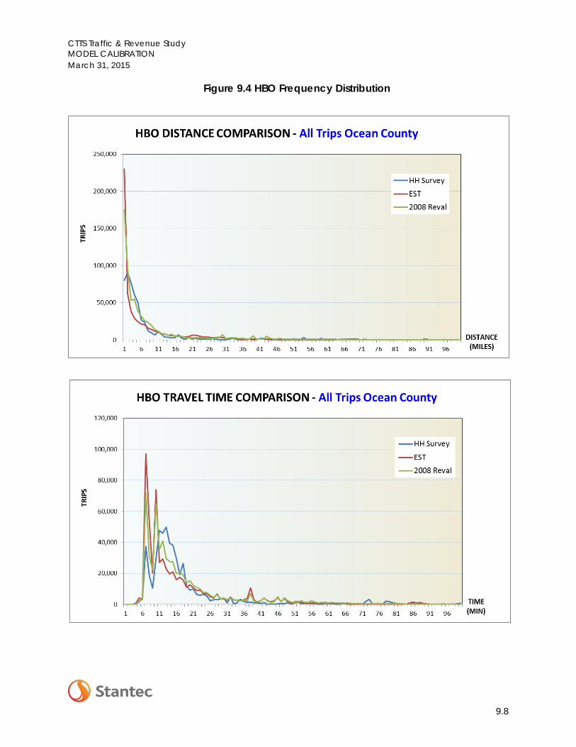
CTTS Traffic & Revenue Study MODEL CALIBRATION March 31, 2015
Figure 9.4 HBO Frequency Distribution
9.8

CTTS Traffic & Revenue Study MODEL CALIBRATION March 31, 2015
Figure 9.5 NHBW Frequency Distribution
9.9
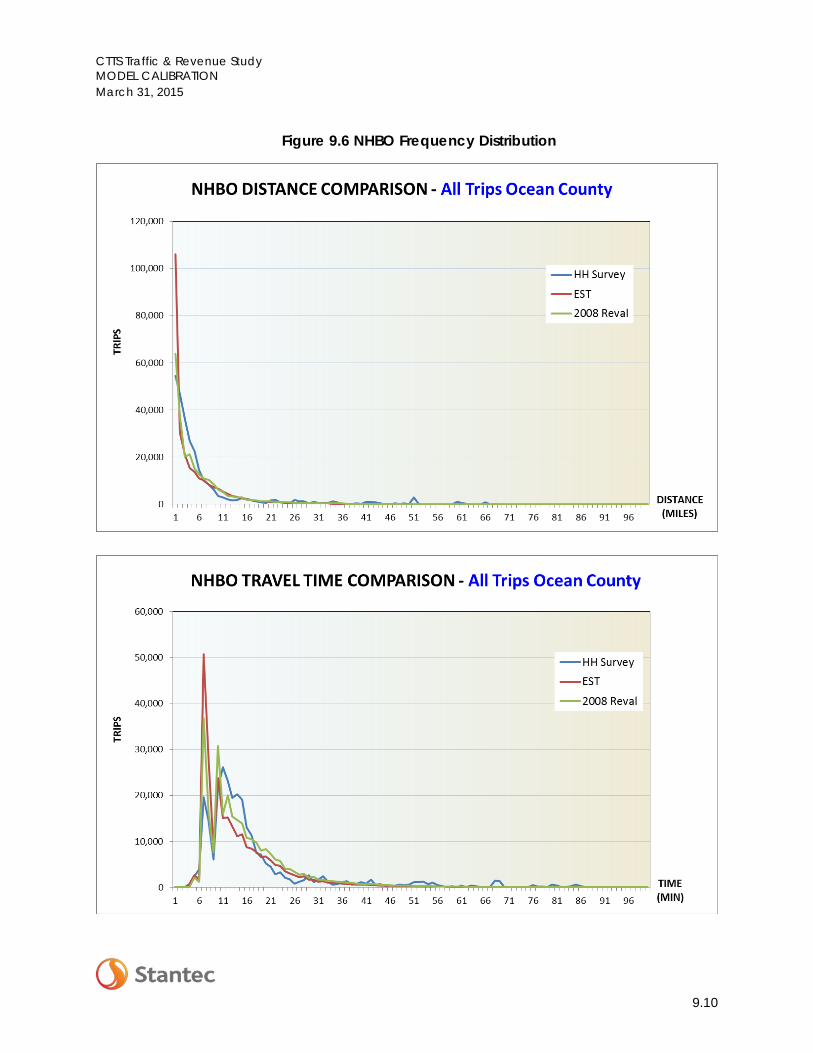
CTTS Traffic & Revenue Study MODEL CALIBRATION March 31, 2015
Figure 9.6 NHBO Frequency Distribution
9.10

CTTS Traffic & Revenue Study MODEL CALIBRATION March 31, 2015
Table 9.9 Average Impedances by Purpose
2010 RHTS 2011 REVAL.(YEAR 2008) ESTIMATED
%DIFF (EST Vs. 2011
REVAL)HBWD 20.5 23.7 24.9 5.2%HBWS 11.6 27.9 26.0 -6.9%HBS 5.4 5.3 5.9 10.6%HBO 7.7 8.9 7.3 -17.1%NHBW 16.1 13.9 12.6 -8.9%NHNW 7.3 5.9 5.0 -15.9%TOTAL 10.8 12.7 12.0 -5.1%
TRIP PURPOSE
AVERAGE DISTANCE (MILES)
2010 RHTS 2011 REVAL.(YEAR 2008) ESTIMATED
%DIFF (EST Vs. 2011
REVAL)HBWD 33.4 39.2 41.3 5.3%HBWS 20.7 45.0 43.7 -2.8%HBS 15.4 14.7 15.5 5.4%HBO 17.2 18.5 17.4 -6.0%NHBW 26.8 25.2 24.8 -1.5%NHNW 16.7 15.7 14.4 -8.6%TOTAL 21.1 24.2 24.0 -1.0%
TRIP PURPOSE
AVERAGE TRAVEL TIME(MINUTES)
2010 RHTS 2011 REVAL.(YEAR 2008) ESTIMATED
%DIFF (EST Vs. 2011
REVAL)HBWD 36.8 36.2 36.2 -0.1%HBWS 33.7 37.3 35.7 -4.2%HBS 21.1 21.6 22.7 5.0%HBO 26.8 28.7 25.3 -11.9%NHBW 36.1 33.0 30.5 -7.4%NHNW 26.2 22.6 20.8 -8.0%TOTAL 29.2 29.3 27.6 -5.9%
TRIP PURPOSE
AVERAGE SPEED(MPH)
9.11

CTTS Traffic & Revenue Study MODEL CALIBRATION March 31, 2015
Ideally, district-to-district trip flow would also help to gauge how close the estimated trip distribution replicated the observed data. However, considering that the RHTS data at-county level is very limited, it is impossible to construct a meaningful trip interchange data. Instead, Stantec developed the percentage production and attraction by district. For this purpose, Ocean County was divided into four districts as shown in Figure 9.7, as follows:
• District 1 – Beach Haven, Eagleswood, Harvey Cedars, Little Egg Harbor, Long Beach, Ship Bottom, Stafford, and Tuckerton
• District 2 – Barnegat, Barnegat Light, Beachwood, Berkeley, Lacey, Lakehurst, Manchester, Ocean, Pine Beach, South Toms River
• District 3 – Bay Head, Brick, Jackson, Lakewood, Mantoloking, Plumsted, Point Pleasant • District 4 – Island Heights, Toms River
Figure 9.7 District Definition
9.12

CTTS Traffic & Revenue Study MODEL CALIBRATION March 31, 2015
Tables 9.10 to 9.15 show the percent distribution comparison by district for each purpose.
Table 9.10 Percent Distribution by District - HBWD
Table 9.11 Percent Distribution by District - HBWS
Table 9.12 Percent Distribution by District - HBS
Table 9.13 Percent Distribution by District – HBO
HBWS
HH SURVEY 2008 REVALIDATION ESTIMATED HH SURVEY 2008
REVALIDATION ESTIMATED
1 10% 9% 12% 9% 9% 12%2 24% 32% 29% 14% 17% 16%3 43% 41% 42% 47% 47% 46%4 22% 19% 18% 30% 28% 27%
Total 100% 100% 100% 100% 100% 100%
DISTRICTPERCENT DISTRIBUTION PRODUCTION PERCENT DISTRIBUTION ATTRACTION
HBWD
HH SURVEY 2008 REVALIDATION ESTIMATED HH SURVEY 2008
REVALIDATION ESTIMATED
1 11% 9% 11% 6% 9% 12%2 34% 31% 28% 14% 18% 16%3 39% 41% 42% 46% 46% 46%4 16% 19% 18% 35% 28% 27%
Total 100% 100% 100% 100% 100% 100%
DISTRICTPERCENT DISTRIBUTION PRODUCTION PERCENT DISTRIBUTION ATTRACTION
HBS
HH SURVEY 2008 REVALIDATION ESTIMATED HH SURVEY 2008
REVALIDATION ESTIMATED
1 11% 8% 10% 14% 10% 10%2 25% 37% 32% 18% 26% 28%3 36% 38% 40% 37% 39% 38%4 28% 17% 17% 32% 25% 24%
Total 100% 100% 100% 100% 100% 100%
DISTRICTPERCENT DISTRIBUTION PRODUCTION PERCENT DISTRIBUTION ATTRACTION
HBO
HH SURVEY 2008 REVALIDATION ESTIMATED HH SURVEY 2008
REVALIDATION ESTIMATED
1 9% 8% 11% 8% 7% 7%2 15% 34% 30% 17% 26% 26%3 50% 40% 42% 49% 44% 46%4 26% 18% 16% 25% 22% 22%
Total 100% 100% 100% 100% 100% 100%
DISTRICTPERCENT DISTRIBUTION PRODUCTION PERCENT DISTRIBUTION ATTRACTION
9.13

CTTS Traffic & Revenue Study MODEL CALIBRATION March 31, 2015
Table 9.14 Percent Distribution by District - NHBW
Table 9.15 Percent Distribution by District - NHBO
9.4 MODE CHOICE
The mode choice model for the OCTM is adopted from the NJRTM-E and the NJ Transit’s North Jersey Travel Demand Forecasting Model (NJTDFM). The mode choice is a typical step within a traditional 4-step travel forecasting model. In this step, trips in each zone-to-zone cell of the person trip table are divided among the different available travel modes. The selection of travel mode is a function of the characteristics of each mode that is available for that particular origin-destination zonal pair and the characteristics of the traveler, the production zone, and the attraction zone. The mathematical function used in the mode choice model to perform this split is known as a nested logit model. Figure 9.8 shows the nesting structure of this model.
NHBW
HH SURVEY 2008 REVALIDATION ESTIMATED HH SURVEY 2008
REVALIDATION ESTIMATED
1 4% 10% 12% 2% 10% 12%2 16% 17% 16% 14% 17% 16%3 46% 44% 44% 50% 44% 44%4 34% 30% 28% 34% 30% 28%
Total 100% 100% 100% 100% 100% 100%
DISTRICTPERCENT DISTRIBUTION PRODUCTION PERCENT DISTRIBUTION ATTRACTION
NHBO
HH SURVEY 2008 REVALIDATION ESTIMATED HH SURVEY 2008
REVALIDATION ESTIMATED
1 12% 10% 12% 12% 10% 12%2 16% 24% 23% 17% 24% 23%3 46% 39% 41% 45% 39% 41%4 26% 27% 24% 26% 27% 24%
Total 100% 100% 100% 100% 100% 100%
DISTRICTPERCENT DISTRIBUTION PRODUCTION PERCENT DISTRIBUTION ATTRACTION
9.14

CTTS Traffic & Revenue Study MODEL CALIBRATION March 31, 2015
Figure 9.8 Nesting Structure for Mode Choice Model
The calibration results are shown in Tables 9.16 to 9.21. It is apparent from both observed and estimated data, that the transit trips in the Ocean County is insignificant.
Table 9.16 Mode Choice Comparison - HBWD
Trips Pct Trips Pct Trips PctSOV 229,980 87.6% 255,448 87.3% 230,753 84.7%
HOV2 11,106 4.2% 25,965 8.9% 30,397 11.2%HOV3 3,950 1.5% 4,116 1.4% 4,906 1.8%HOV4 7,528 2.9% 3,474 1.2% 3,929 1.4%
Walk-Transit 477 0.2% 723 0.2% 367 0.1%Drive-Transit 9,630 3.7% 2,949 1.0% 2,053 0.8%
TOTAL 262,671 100.0% 292,675 100.0% 272,404 100.0%
MODEHBWD (Person Trips)2008 Revalidation Estimated2010 RHTS
9.15

CTTS Traffic & Revenue Study MODEL CALIBRATION March 31, 2015
Table 9.17 Mode Choice Comparison - HBWS
Table 9.18 Mode Choice Comparison - HBS
Table 9.19 Mode Choice Comparison - HBO
Trips Pct Trips Pct Trips PctSOV 72,202 73.1% 90,252 84.7% 82,936 83.5%
HOV2 12,913 13.1% 9,090 8.5% 11,409 11.5%HOV3 10,114 10.2% 1,799 1.7% 1,916 1.9%HOV4 3,504 3.5% 1,399 1.3% 1,528 1.5%
Walk-Transit 0 0.0% 848 0.8% 238 0.2%Drive-Transit 0 0.0% 3,173 3.0% 1,275 1.3%
TOTAL 98,733 100.0% 106,561 100.0% 99,303 100.0%
HBWS (Person Trips)2010 RHTS 2008 Revalidation EstimatedMODE
Trips Pct Trips Pct Trips PctSOV 85,040 53.8% 76,123 44.7% 70,779 44.8%
HOV2 61,780 39.1% 66,912 39.3% 61,988 39.3%HOV3 7,270 4.6% 13,432 7.9% 12,432 7.9%HOV4 3,488 2.2% 13,599 8.0% 12,585 8.0%
Walk-Transit 413 0.3% 71 0.0% 35 0.0%Drive-Transit 0 0.0% 16 0.0% 6 0.0%
TOTAL 157,991 100.0% 170,153 100.0% 157,824 100.0%
MODE 2010 RHTS 2008 Revalidation EstimatedHBS (Person Trips)
Trips Pct Trips Pct Trips PctSOV 205,267 40.5% 264,772 42.3% 208,404 41.1%
HOV2 164,889 32.5% 211,138 33.7% 173,776 34.3%HOV3 65,279 12.9% 77,508 12.4% 63,802 12.6%HOV4 70,051 13.8% 71,632 11.4% 59,195 11.7%
Walk-Transit 1,763 0.3% 374 0.1% 250 0.0%Drive-Transit 0 0.0% 852 0.1% 1,101 0.2%
TOTAL 507,249 100.0% 626,276 100.0% 506,528 100.0%
2010 RHTS 2008 Revalidation EstimatedMODEHBO (Person Trips)
9.16

CTTS Traffic & Revenue Study MODEL CALIBRATION March 31, 2015
Table 9.20 Mode Choice Comparison - NHBW
Table 9.21 Mode Choice Comparison - NHBO
9.5 HIGHWAY ASSIGNMENT
The highway assignment calibration focused on the standard comparison of volumes and VMT by various classification, such as facility type and area type. The assignment calibration also focused on the screenline volumes and the distribution of the traffic among the roadways that construed the screenlines. The calibration also reviewed the traffic along the Garden State Parkway, the major limited-access facility that crosses the Ocean County in the north-south direction.
Tables 9.22 and 9.23 show the volume and VMT comparison between observed count data and estimated volumes by facility type and by area type. At the regional, the estimated volume is approximately within three percent of the observed data. At facility type level, the ratios are generally within ten percent, except for two categories where the counts are very limited. At area type level, the estimated volumes are within three percent of the observed traffic counts. At more disaggregated level, the differences are more pronounced although they are generally within reasonable tolerance as shown in Tables 9.24 and 9.25.
Trips Pct Trips Pct Trips PctSOV 89,127 84.7% 61,235 76.3% 82,550 75.4%
HOV2 9,952 9.5% 10,871 13.5% 15,547 14.2%HOV3 4,168 4.0% 5,313 6.6% 7,440 6.8%HOV4 1,714 1.6% 2,618 3.3% 3,766 3.4%
Walk-Transit 245 0.2% 170 0.2% 138 0.1%Drive-Transit 0 0.0% 62 0.1% 75 0.1%
TOTAL 105,206 100.0% 80,268 100.0% 109,515 100.0%
2010 RHTSMODENHBW (Person Trips)2008 Revalidation Estimated
Trips Pct Trips Pct Trips PctSOV 121,848 46.5% 79,953 35.4% 120,111 46.8%
HOV2 96,443 36.8% 83,963 37.2% 77,467 30.2%HOV3 23,447 9.0% 42,081 18.6% 42,168 16.4%HOV4 18,502 7.1% 19,737 8.7% 16,778 6.5%
Walk-Transit 1,577 0.6% 44 0.0% 172 0.1%Drive-Transit 0 0.0% 11 0.0% 59 0.0%
TOTAL 261,817 100.0% 225,789 100.0% 256,755 100.0%
NHBO (Person Trips)2010 RHTS 2008 Revalidation EstimatedMODE
9.17

CTTS Traffic & Revenue Study MODEL CALIBRATION March 31, 2015
Table 9.22 Volume Comparison by Facility Type and by Area Type
Table 9.23 VMT Comparison by Facility Type and by Area Type
OBSERVED ESTIMATED EST/OBS COUNTSLimited-Access Facility 1,987,944 1,919,450 0.97 57Expressway 70,394 78,017 1.11 4Principal Arterial Divided 432,846 461,363 1.07 30Principal Arterial Undivided 918,859 898,826 0.98 96Minor Arterial Divided 38,298 32,251 0.84 4Minor Arterial Undivided 1,081,585 1,025,965 0.95 202Minor Arterials 462,332 424,416 0.92 142Collector/Local 167,625 162,291 0.97 54
TOTAL 5,159,883 5,002,579 0.97 589
BY AREA TYPE
OBSERVED ESTIMATED EST/OBS COUNTSUrban 177,635 173,042 0.97 14
Suburban 4,596,118 4,445,463 0.97 505Rural 386,130 384,074 0.99 70TOTAL 5,159,883 5,002,579 0.97 589
FACILITY TYPEVOLUME
AREA TYPEVOLUME
BY FACILITY TYPE
OBSERVED ESTIMATED EST/OBSLimited-Access Facility 2,538,454 2,484,880 0.98Expressway 79,229 94,804 1.20Principal Arterial Divided 381,003 414,055 1.09Principal Arterial Undivided 539,799 578,708 1.07Minor Arterial Divided 23,193 19,762 0.85Minor Arterial Undivided 932,434 898,981 0.96Minor Arterials 273,583 246,441 0.90Collector/Local 87,881 88,115 1.00
TOTAL 4,855,576 4,825,746 0.99
BY AREA TYPE
OBSERVED ESTIMATED EST/OBSUrban 92,209 87,518 0.95
Suburban 4,131,227 4,115,123 1.00Rural 632,140 623,105 0.99TOTAL 4,855,576 4,825,746 0.99
FACILITY TYPEVOLUME
AREA TYPEVOLUME
9.18

CTTS Traffic & Revenue Study MODEL CALIBRATION March 31, 2015
Table 9.24 Volume Comparison by Facility Type and Area Type
OBSERVED VOLUME
Urban Suburban Rural TotalLimited-Access Facility -- 1,811,904 176,040 1,987,944Expressway -- 70,394 -- 70,394Principal Arterial Divided 66,904 365,942 -- 432,846Principal Arterial Undivided 93,614 803,796 21,449 918,859Minor Arterial Divided -- 38,298 -- 38,298Minor Arterial Undivided 17,117 896,593 167,875 1,081,585Minor Arterials -- 442,389 19,943 462,332Collector/Local -- 166,802 823 167,625
TOTAL 177,635 4,596,118 386,130 5,159,883
ESTIMATED VOLUME
Urban Suburban Rural TotalLimited-Access Facility -- 1,746,211 173,239 1,919,450Expressway -- 78,017 -- 78,017Principal Arterial Divided 60,634 400,729 -- 461,363Principal Arterial Undivided 96,276 776,019 26,531 898,826Minor Arterial Divided -- 32,251 -- 32,251Minor Arterial Undivided 16,132 844,680 165,153 1,025,965Minor Arterials -- 405,824 18,592 424,416Collector/Local -- 161,732 559 162,291
TOTAL 173,042 4,445,463 384,074 5,002,579
ESTIMATED VOLUME/OBSERVED VOLUME
Urban Suburban Rural TotalLimited-Access Facility -- 0.96 0.98 0.97Expressway -- 1.11 -- 1.11Principal Arterial Divided 0.91 1.10 -- 1.07Principal Arterial Undivided 1.03 0.97 1.24 0.98Minor Arterial Divided -- 0.84 -- 0.84Minor Arterial Undivided 0.94 0.94 0.98 0.95Minor Arterials -- 0.92 0.93 0.92Collector/Local -- 0.97 0.68 0.97
TOTAL 0.97 0.97 0.99 0.97
TOTAL COUNTS
Urban Suburban Rural TotalLimited-Access Facility -- 49 8 57Expressway -- 4 -- 4Principal Arterial Divided 4 26 -- 30Principal Arterial Undivided 8 84 4 96Minor Arterial Divided -- 4 -- 4Minor Arterial Undivided 2 162 38 202Minor Arterials -- 124 18 142Collector/Local -- 52 2 54
TOTAL 14 505 70 589
FACILITY TYPEAREA TYPE
FACILITY TYPEAREA TYPE
FACILITY TYPEAREA TYPE
FACILITY TYPEAREA TYPE
9.19

CTTS Traffic & Revenue Study MODEL CALIBRATION March 31, 2015
Table 9.25 VMT Comparison by Facility Type and Area Type
OBSERVED VMT
Urban Suburban Rural TotalLimited-Access Facility -- 2,226,036 312,418 2,538,454Expressway -- 79,229 -- 79,229Principal Arterial Divided 60,760 320,243 -- 381,003Principal Arterial Undivided 27,769 484,915 27,115 539,799Minor Arterial Divided -- 23,193 -- 23,193Minor Arterial Undivided 3,680 653,656 275,098 932,434Minor Arterials -- 257,474 16,109 273,583Collector/Local -- 86,481 1,400 87,881
TOTAL 92,209 4,131,227 632,140 4,855,576
ESTIMATED VMT
Urban Suburban Rural TotalLimited-Access Facility -- 2,182,977 301,903 2,484,880Expressway -- 94,804 -- 94,804Principal Arterial Divided 60,123 353,932 -- 414,055Principal Arterial Undivided 23,927 520,885 33,896 578,708Minor Arterial Divided -- 19,762 -- 19,762Minor Arterial Undivided 3,468 624,839 270,674 898,981Minor Arterials -- 230,523 15,918 246,441Collector/Local -- 87,401 714 88,115
TOTAL 87,518 4,115,123 623,105 4,825,746
ESTIMATED VOLUME/OBSERVED VMT
Urban Suburban Rural TotalLimited-Access Facility -- 0.98 0.97 0.98Expressway -- 1.20 -- 1.20Principal Arterial Divided 0.99 1.11 -- 1.09Principal Arterial Undivided 0.86 1.07 1.25 1.07Minor Arterial Divided -- 0.85 -- 0.85Minor Arterial Undivided 0.94 0.96 0.98 0.96Minor Arterials -- 0.90 0.99 0.90Collector/Local -- 1.01 0.51 1.00
TOTAL 0.95 1.00 0.99 0.99
TOTAL COUNTS
Urban Suburban Rural TotalLimited-Access Facility -- 49 8 57Expressway -- 4 -- 4Principal Arterial Divided 4 26 -- 30Principal Arterial Undivided 8 84 4 96Minor Arterial Divided -- 4 -- 4Minor Arterial Undivided 2 162 38 202Minor Arterials -- 124 18 142Collector/Local -- 52 2 54
TOTAL 14 505 70 589
FACILITY TYPEAREA TYPE
FACILITY TYPEAREA TYPE
FACILITY TYPEAREA TYPE
FACILITY TYPEAREA TYPE
9.20

CTTS Traffic & Revenue Study MODEL CALIBRATION March 31, 2015
The next comparison is by screenline. Figure 9.9 shows the screenline locations for this study, while Table 9.26 shows the total traffic by screenline. The comparison indicates that the estimated volumes are generally lower than the observed traffic, except for screenline no. 6.
Figure 9.9 Screenline Definition
9.21

CTTS Traffic & Revenue Study MODEL CALIBRATION March 31, 2015
Table 9.26 Total Screenline Traffic Comparison
The distribution of screenline traffic among the roadways is shown in Table 9.27. At this level, the difference between observed and estimated traffic is more pronounced.
Table 9.27 Total Screenline Traffic Comparison
Counts Estimated % Diff1 271,854 242,326 -10.9%2 101,084 95,177 -5.8%3 95,786 92,632 -3.3%4 83,551 75,560 -9.6%5 180,332 168,260 -6.7%6 86,877 93,739 7.9%7 327,339 318,063 -2.8%
SCREENLINE NO Total Screenline Traffic
Counts Dist. Estimated Dist.RT 539/WHITING NEW EGYPT RD 11,450 4.2% 9,266 3.8%RT 547 11,448 4.2% 14,939 6.2%NJ 70 20,586 7.6% 18,238 7.5%RT 571 19,288 7.1% 16,112 6.6%RT 527 15,059 5.5% 7,391 3.0%US 9 27,950 10.3% 24,999 10.3%GARDEN STATE PARKWAY 86,100 31.7% 86,433 35.7%OLD FREEHOLD RD 16,606 6.1% 20,422 8.4%RT 549/HOOPER AVE 42,984 15.8% 30,849 12.7%NJ 35 20,383 7.5% 13,678 5.6%
TOTAL 271,854 100.0% 242,326 100.0%RT 539 6,506 6.4% 9,184 9.6%GARDEN STATE PARKWAY 75,900 75.1% 74,204 78.0%US 9 18,678 18.5% 11,790 12.4%
TOTAL 101,084 100.0% 95,177 100.0%RT 539 4,112 4.3% 9,236 10.0%NJ 72 11,718 12.2% 9,494 10.2%RT 532 1,733 1.8% 2,356 2.5%GARDEN STATE PARKWAY 63,380 66.2% 62,237 67.2%US 9 14,843 15.5% 9,308 10.0%
TOTAL 95,786 100.0% 92,632 100.0%NJ 35 19,359 23.2% 26,927 35.6%NJ 88 21,887 26.2% 13,057 17.3%BRIDGE AVE 10,601 12.7% 8,171 10.8%RT 528 9,202 11.0% 6,501 8.6%NJ 37 22,502 26.9% 20,903 27.7%
TOTAL 83,551 100.0% 75,560 100.0%I-195 35,370 19.6% 40,619 24.1%CHANDLER RD 3,298 1.8% 1,511 0.9%HYSON RD 3,972 2.2% 5,481 3.3%RT 526/COUNTY LINE RD 12,700 7.0% 8,908 5.3%BENNETTS MILLS RD 8,817 4.9% 8,969 5.3%RT 528/E VETERAN RD 7,269 4.0% 4,577 2.7%RT 527 4,875 2.7% 8,262 4.9%RT 547 12,021 6.7% 11,448 6.8%NJ 70 23,773 13.2% 20,513 12.2%RT 571 11,293 6.3% 17,672 10.5%NJ 37 31,870 17.7% 20,472 12.2%RT 530/ PINEWALD KESWICK RD 8,114 4.5% 7,362 4.4%RT 614/LACEY RD 4,613 2.6% 2,178 1.3%NJ 72 11,718 6.5% 9,494 5.6%RT 532 628 0.3% 794 0.5%
TOTAL 180,332 100.0% 168,260 100.0%
Scre
enlin
e 5
LOCATION Validation Year (2010)
Scre
enlin
e 1
Scrn
ln 2
Scre
enlin
e 3
Scre
enlin
e 4
9.22

CTTS Traffic & Revenue Study MODEL CALIBRATION March 31, 2015
Table 9.27 - Continued
The final comparison for the highway assignment calibration is traffic along the Garden State Parkway. The summary of this comparison is shown in Table 9.28. While the difference on each segment is more pronounced, the difference of the total segments is within three percent.
Counts Dist. Estimated Dist.MONMOUTH RD 6,294 7.2% 12,526 13.4%RT 528 4,050 4.7% 2,570 2.7%RT 616 4,950 5.7% 5,359 5.7%BUNTING BRIDGE RD 1,429 1.6% 173 0.2%NJ 70 11,268 13.0% 14,169 15.1%NJ 72 8,167 9.4% 9,845 10.5%GARDEN STATE PARKWAY 40,300 46.4% 41,308 44.1%RT 654/STAGE RD 823 0.9% 559 0.6%US 9 9,596 11.0% 7,229 7.7%
TOTAL 86,877 100.0% 93,739 100.0%RT 539 FORKED RIVER RD 12,394 3.8% 7,264 2.3%RT 537 18,420 5.6% 13,443 4.2%RT 571 8,222 2.5% 9,700 3.0%RT 527/CEDAR SWAMP RD 8,047 2.5% 4,930 1.5%HARMONY RD 2,145 0.7% 4,522 1.4%OCEAN COUNTY 638/JACKSON MILLS RD 8,286 2.5% 4,463 1.4%OCEAN COUNTY 641 3,298 1.0% 1,511 0.5%FORT PLAINT RD 5,572 1.7% 11,065 3.5%US 9 44,744 13.7% 42,081 13.2%GEORGIA TAVERN RD 4,709 1.4% 2,914 0.9%RT 524A/SQUANKUM YELLOWBROOK RD 7,011 2.1% 6,526 2.1%RT 524 8,853 2.7% 4,964 1.6%GARDEN STATE PARKWAY 125,530 38.3% 114,996 36.2%NJ 34 40,286 12.3% 66,720 21.0%NJ 35 19,701 6.0% 12,458 3.9%NJ 71 10,121 3.1% 10,505 3.3%
TOTAL 327,339 100.0% 318,063 100.0%
LOCATION+K6:P34 Validation Year (2010)Sc
reen
line
6Sc
reen
line
7
9.23

CTTS Traffic & Revenue Study MODEL CALIBRATION March 31, 2015
Table 9.28 Traffic Comparison Along Garden State Parkway
9.6 TRANSIT ASSIGNMENT CALIBRATION
Ocean County has only limited transit lines that serve the county. Most of the buses provided by the NJ Transit and they usually serve inter-county trips. The only local service, by Ocean Ride, included in this analysis is Toms River Connection. Table 9.29 shows the ridership comparison by lines.
Table 9.29 Transit Ridership Comparison by Line
Observed Estimated %DiffNB 22,650 24,436 7.9%SB 22,340 22,041 -1.3%NB 25,600 28,261 10.4%SB 25,560 27,484 7.5%NB 32,860 32,143 -2.2%SB 30,520 30,094 -1.4%NB 38,440 37,494 -2.5%SB 37,460 36,709 -2.0%NB 38,440 39,924 3.9%SB 37,460 36,068 -3.7%NB 40,250 40,866 1.5%SB 38,170 36,558 -4.2%NB 55,610 56,027 0.7%SB 54,880 59,263 8.0%NB 49,790 53,118 6.7%SB 51,180 54,947 7.4%NB 52,100 49,281 -5.4%SB 54,520 49,819 -8.6%NB 44,540 46,266 3.9%SB 41,560 40,168 -3.4%NB 61,630 52,161 -15.4%SB 59,740 56,832 -4.9%NB 53,880 49,118 -8.8%SB 51,370 47,720 -7.1%NB 61,430 58,462 -4.8%SB 64,100 56,534 -11.8%NB 577,220 567,556 -1.7%SB 568,860 554,237 -2.6%Total
Between Interchange 67 and Interchange 69 (Rt. 532)
Between Interchange 69 and Interchange 74 (Lacey Rd)
Between Interchange 74 and Interchange 77 (Forrest Hill Parkway)
Between Interchange 77 and Interchange 80 (US 9/Rt. 530)
Between Interchange 80 and Interchange 81 (Rt. 527)
Between Interchange 81 and Interchange 82 (Rt. 37)
Between Interchange 82 and Interchange 83 (Rt. 9)
Between Interchange 83 and Interchange 89 (Rt. 70/Rt. 528)
Between Interchange 89 and Interchange 90 (Rt. 549)
Between Interchange 90 and Interchange 91 (Burnt Tavern Rd.)
Between Interchange 91 and Interchange 98 (Rt. 34)
Location Direction Daily Traffic Volume
Between Interchange 58 (Rt. 539) and Interchange 63 (Rt. 72)
Between Interchange 63 and Interchange 67 (Rt. 554)
Observed Estimated137 909 745139 471 111317 86 38319 151 103559 761 21264 29 1267 216 192
Toms River 369 453
Line Name Ridership
9.24

CTTS Traffic & Revenue Study ADDITIONAL FEATURES March 31, 2015
10.0 ADDITIONAL FEATURES
10.1 SEASONAL MODEL
The seasonal model was developed to capture additional traffic demand for people traveling to the New Jersey shores during the summer months. During the course of the project, it was decided that the seasonal traffic model would estimate the in-bound traffic (heading to the shores) on a high Summer Friday or Saturday, and the out-bound traffic (returning home) on Sunday.
The increase of summer traffic can be attributed to two categories:
• The increase of local activities. • The in-flux of long-distance trips from nearby regions, such as New York City, Philadelphia,
Trenton, and South Jersey. The increase of local-activities is assumed to be proportional with the vacation housing available in the area. Table 10.1 provides the percentage of seasonal housing by municipality. The data was obtained from the 2010 Housing Units Summary from the Census website. The percentage of vacation housing units were then converted from MCD-Level to Zonal-Level using an MCD-Zones equivalency table developed for this model.
The additional traffic from the local trips is calculated using the following formula:
Additional Local Trips for i-j cell = Average Daily Trips * the average of percent vacation housing units at location i and j
Only a portion of these trips is assumed to occur. Therefore, an adjustment factor is applied to these local trips. Currently, the factor is set to 0.50. The factor was determined with a trial and error approach to get the estimated trips replicating the very limited observed data. Please note that currently, the model is not calibrated due to lack of the available data.
The second component of the seasonal model is the in-flux on long distance trips. For the purpose of this model, Stantec assumed that there are four origin points for these trips:
• Route 72 for the western market such as Philadelphia region. • GSP near Asbury Park or Toms River for the northern market, such as NYC and North
Jersey. • GSP near New Gretna for southern market, such as South Jersey Region. • I-195 for the western market such Trenton and Central Jersey.
Figure 10.1 shows the proximity of these locations, while Figure 10.2 shows the zonal representation of these locations in the highway network.
10.1

CTTS Traffic & Revenue Study ADDITIONAL FEATURES March 31, 2015
Table 10.1 Vacation Housing Percentage by MCD in Ocean County
MCDVacation House
PercentageBarnegat 0.0%Barnegat Light 74.0%Bay Head 46.0%Beach Haven 75.0%Beachwood 0.0%Berkeley 9.0%Brick 7.0%Eagleswood 17.0%Harvey Cedars 76.0%Island Heights 0.0%Jackson 0.0%Lacey 0.0%Lakehurst 0.0%Lakewood 0.0%Lavallette 59.0%Little Egg Harbor 15.0%Long Beach 80.0%Manchester 0.0%Mantoloking 42.0%Ocean 16.0%Ocean Gate 30.0%Pine Beach 0.0%Plumsted 0.0%Point Pleasant 0.0%Point Pleasant Beach 32.0%Seaside Heights 40.0%Seaside Park 63.0%Ship Bottom 70.0%South Toms River 0.0%Stafford 20.0%Surf City 72.0%Toms River 15.0%Tuckerton 23.0%
10.2

CTTS Traffic & Revenue Study ADDITIONAL FEATURES March 31, 2015
Figure 10.1 Screenline Definition
The four seasonal TAZs are as follows:
• Zone 1643 - represents the origin point for the western market such Trenton and Central Jersey.
10.3

CTTS Traffic & Revenue Study ADDITIONAL FEATURES March 31, 2015
• Zone 1644 – represents the origin point of the southern market, such as South Jersey Region.
• Zone 1645 – represents the origin point of the western market such as Philadelphia region. • Zone 1646 – represents the origin point of the northern market, such as NYC and North
Jersey.
Figure 10.2 Seasonal TAZ Representation
10.4

CTTS Traffic & Revenue Study ADDITIONAL FEATURES March 31, 2015
As the first step of the long-haul seasonal traffic estimation, Stantec gathered traffic count information from NJDOT’s permanent stations and Garden State Parkway that can be used as proxy for these locations. There were very limited traffic counts that can be used for this purpose, since the counts should have both average daily counts, as well as counts for summer months by direction. Table 10.2 shows the comparison between high summer traffic volumes and AADT for the selected locations. Since there is no permanent count available on I-195, Stantec assumed that the western market from Trenton and Central Jersey is the same as the market from the South Jersey Region. It should also be noted that the 2013 counts on Garden State Parkway was used as proxy for the 2010 due to the availability of the data during the analysis.
Table 10.2 High Summer Month and AADT Traffic Comparison
The average additional summer traffic from Table 10.2 was used as the base for the long-haul trip production, and is summarized in Table 10.3. Additional adjustment factors were added to account for the discrepancy between the seasonal TAZ locations (shown in Figure 10-2) and the locations of the count, such that the estimated additional summer traffic replicate the observed data. The adjustment factors are listed in Table 10.4.
Table 10.3 Long-Haul In-Bound Trip Origin
Table 10.4 Adjustment Factors In-Bound Trip Origin
High Summer Volume AADT Additional
Summer TrafficHigh Summer
Volume AADT Additional Summer Traffic
Rt. 72 Between Four Mile Road and Pakimpond Road
8,747 4,714 4,033 9,266 4,714 4,552 4,293
GSP at Toms River 65,903 42,288 23,615 66,153 45,735 20,418 22,017GSP at New Gretna 27,700 20,139 7,561 26,840 19,515 7,325 7,443
In-Bound Out-BoundLocation
Average Additional
Summer Traffic
North (GSP @ Toms River) 22,017West (Rt. 72) 4,293
South (GSP @ New Graetna) 7,443West (I-195) - assume similar to New
Gretna7,443
LocationAverage
Additional Summer Traffic
North (GSP @ Toms River) 1.24West (Rt. 72) 1.42
South (GSP @ New Graetna) 1.90West (I-195) - assume similar to New
Gretna1.90
LocationProduction Adjustment
Factors
10.5

CTTS Traffic & Revenue Study ADDITIONAL FEATURES March 31, 2015
Stantec suggests that additional data are collected for future use. Full-calibration can be performed when those new traffic counts are available in the future, and all parameters and adjustment factors can also be adjusted accordingly based on the new data.
The attraction of the long-haul in-bound summer traffic was also estimated based on vacation housing units. The distribution of the trips from the four production zones to all potential attraction zones, zones with vacation housing, was performed using a simple gravity model with trips balanced to production.
The out-bound trips, which represent the return trips on Sunday, were calculated using similar approach as the in-bound trips. However, the production and attraction were reversed and the trips are balanced to attraction.
The daily seasonal trips were distributed into four time-of-day, AM, PM, Midday, and Night using the time of day factors developed from the GSP hourly summer traffic counts at Toms River Plaza on a summer day. The time-of-day factors are shown in Table 10.5
Table 10.5 Time-Of-Day Factors for Seasonal Trips
Table 10.6 shows traffic comparison between traffic counts and the estimated volumes at selected locations, while Figure 10.2 shows the AM-peak in-bound traffic. The results in Table 10.6 indicate that the estimated seasonal traffic on GSP is reasonably close to the traffic counts at Toms River Plaza. The estimated volume at New Gretna Plaza is approximately 12% higher than the traffic counts, while at Barnegat (SB), it is approximately 13% lower. The estimated traffic at Route 72 is approximately 40% and 20% higher for in-bound and out-bound traffic, respectively. These high percentages are partly due to small additional volumes, such that the small changes in volumes generated higher percentage numbers. It should be noted that the seasonal model application will create two loaded highway networks for each time period and daily. Only traffic volumes on their corresponding direction should be considered. For example, only in-bound traffic volumes, heading to the New Jersey Shores, will be obtained from the in-bound loaded network, and vice versa.
Table 10.6 Seasonal Traffic Comparison
Toll Location 6-9 AM 9-3 PM 3-6 PM 6-6 AMAM MD PM NT TOTAL
Toms River NB (OB) 4,439 25,705 12,106 23,903 66,153Toms River SB (IB) 8,194 27,407 13,614 16,688 65,903Toms River NB (OB) 6.7% 38.9% 18.3% 36.1%Toms River SB (IB) 12.4% 41.6% 20.7% 25.3%
Observed Estimated Diff Observed Estimated Diff Observed Estimated % DiffInbound (EB) 4,714 8,132 3,418 8,747 13,928 5,181 4,033 5,795 44%Outbound (WB) 4,714 11,512 6,798 9,266 17,000 7,734 4,552 5,488 21%Inbound (SB) 42,288 40,168 -2,120 65,903 64,479 -1,424 23,615 24,311 3%Outbound (NB) 45,735 46,266 531 66,153 66,875 722 20,418 20,609 1%
GSP @ New Graetna NB Inbound (NB) 26,250 20,269 -5,981 36,637 31,936 -4,701 10,387 11,667 12%GSP @ Barnegat SB Inbound (NB) 42,288 30,094 -12,194 65,903 50,550 -15,353 23,615 20,456 -13%
Rt. 72 Between Four Mile Rd. & Pakimpond Rd.
GSP @ Toms River Plaza
Location DirectionAADT Seasonal Traffic Additional Seasonal Traffic
10.6

CTTS Traffic & Revenue Study ADDITIONAL FEATURES March 31, 2015
Figure 10.3 Example of AM-Peak Seasonal In-Bound traffic
For future year analysis, Stantec assumes that the long-haul traffic grows at a rate of 0.5% per year. This assumption was derived from a historical traffic count data from 2009 to 2014 along the GSP at three mainline locations including New Gretna, Barnegat, and Toms River. Table 10.7 shows the historical growth rates at these locations. Hurricane Sandy hit the Jersey Shore in 2012 which impacted the travel to Jersey Shore during that year and 2013. To minimize the impact of hurricane Sandy, the growth rate was calculated for two periods:
• Between 2009 and 2011, prior to Hurricane Sandy, and • Between 2009 and 2014, to reflect a long term growth.
10.7

CTTS Traffic & Revenue Study ADDITIONAL FEATURES March 31, 2015
Table 10.7 Historical Growth Rate along GSP
Note: (1) ACGR = Annual Compounded Growth Rate
The Garden State Parkway experienced a decline in traffic between 2009 and 2011. This is presumably due to the increase of fuel cost between those years that discouraged people from making discretionary travels. The long term growth rates between 2009 and 2014, indicate positive growth rates at Barnegat and Toms River Plazas, and negative rates at New Gretna Plaza. The total growth rate is approximately 0.1% per year. Considering that there is still an on-going recovery effort from Hurricane Sandy, Stantec assumed a higher annual growth rate, at 0.5% per year, for future year analysis. This growth rate assumption can be revisited upon the completion of the recovery effort, and as more historical data becomes available.
To account for the growth, the analyst has to input the analysis year for the seasonal model. The year has to be input into SEASON_YR key variable as shown in Figure 10.4.
Figure 10.4 Example of AM-Peak Seasonal In-Bound traffic
2009 2010 2011 2012 2013 2014 2009-2011 2009-2014NB 20,470 20,040 19,410 19,951 19,835 19,436 -2.6% -1.0%SB 20,620 20,260 20,020 20,588 20,649 20,058 -1.5% -0.6%NB 33,190 32,860 31,640 33,889 34,482 34,199 -2.4% 0.6%SB 31,630 30,520 29,700 31,819 32,375 32,112 -3.1% 0.3%NB 45,100 44,540 43,200 44,865 44,960 45,735 -2.1% 0.3%SB 42,070 41,560 40,510 42,907 42,775 42,288 -1.9% 0.1%NB 98,760 97,440 94,250 98,705 99,277 99,370 -2.3% 0.1%SB 94,320 92,340 90,230 95,314 95,799 94,458 -2.2% 0.0%
AVERAGE DAILY TRAFFICPLAZA LOCATION DIR % ACGR(1)
Total
New Gretna
Barnegat
Toms River
10.8

CTTS Traffic & Revenue Study ADDITIONAL FEATURES March 31, 2015
10.2 CRITICAL LOCATIONS AND FUTURE YEARS FORECAST
As part of the 2010 calibration effort, Stantec also reviewed the locations of roadways that experience some level of congestion. Figure 10.5 shows an example of the congested locations estimated by the model during the AM Peak Hour period (6AM – 9 AM).
Figure 10.5 Example of AM-Peak Congestion Level
10.9

CTTS Traffic & Revenue Study ADDITIONAL FEATURES March 31, 2015
The color legend of this Figure is as follows:
• Brown – Level of Service F (V/C >1.0) • Red – Level of Service E (V/C=0.90-1.00) • Dark Orange – Level of Service D (V/C=0.75-0.90) • Light Orange – Level of Service C (V/C=0.50-0.75) • Green – Level of Service A & B (V/C<0.50)
Figure 10.6 shows a typical Wednesday morning traffic around 7:30 AM from Google Maps.
Figure 10.6 Typical Wednesday Morning Traffic in Ocean County
Both figures show some congestion on the Garden State Parkway, even though the model estimates show a higher level of congestion along GSP. Google Map shows slightly more
10.10

CTTS Traffic & Revenue Study ADDITIONAL FEATURES March 31, 2015
congestion on Route 9 compared to the model estimates. Focusing on the Toms River area, the model estimated higher congestion along Old Freehold Road, North Bay Avenue, and Route 527, while underestimated the congestion along Hoopers Avenue and Route 37 as shown in Figure 10.7.
Figure 10.7 Congestion Level in Toms River during AM Peak.
In addition to congestion check, Stantec also reviewed the estimated daily traffic volumes along US 9 and compared them to the observed data. Figure 10.8 shows the comparison of traffic counts and model estimated daily volumes. The estimated traffic volumes on the southern section, south of Veterans Blvd in Berkeley Township, are generally lower than the observed traffic counts. However, the estimated volumes are closer to the observed counts north of Veterans Blvd, and in segments even higher than the counts. The traffic comparison indicates that the estimated traffic along US 9 corridor is comparable to the count data.
Table 10.8 lists the important roadway locations where the AM Peak congestion was estimated by the 2010 model year results. The congestion was only measured by the roadways’ V/C ratios. However, it should be noted that there are other factors that may impact the roadway congestion and could not be estimated precisely by the regional model, such as:
• Intersection delay – the regional and county models are macroscopic models, and they are not designed to estimate detailed operational characteristics of the roadways, even though some traffic control device modeling features were included in the models. The model is usually geared toward a broader analysis and general roadway trends in the study region. For corridor-level studies with its detailed operational characteristics, a finer
10.11

CTTS Traffic & Revenue Study ADDITIONAL FEATURES March 31, 2015
analysis or microscopic analysis is required, such as traffic simulation studies. The simulation analysis can use a subarea trip tables that are derived from the regional model.
• Peak-hour congestion level – the regional model was designed to cover peak periods that extend more than one hour period. In the Ocean County Model, the peak periods, both AM and PM, are defined as a three-our period as discussed in Section 9.1. If the peak-spreading of traffic in a corridor is significantly less than three hours, the peak period V/C ratios will understate the congestion during the peak hour.
• Congestion caused by traffic entering and exiting driveways of commercial establishments. This type of congestion
Figure 10.8 Daily Traffic Comparison Along Route 9
10.12

CTTS Traffic & Revenue Study ADDITIONAL FEATURES March 31, 2015
Table 10.8 Estimated Critical Locations in 2010
As part of this project, Stantec performed two future years model scenarios, 2025 and 2040. Several projects obtained from the FY2014 Conformity Project List were applied to the future highway networks. The list of the projects is shown on Table 10.9. In addition two project log files for Church Road Extension and North Bay Extension Projects were also prepared, although they are not applied to the network. The two log files are stored in the “Future Projects” sub-folder in the OCTM2013 folder.
Table 10.9 Future Projects
No DB Number DescriptionsEstimated
Completion Year(1)
1 GSP1402 GSP Widening, Interchange 48 to Interchange 63 from 2 lanes to 3 lanes in each direction. 2013/2014
2 97080A Intersection improvements at Route 9 and Lacey Road, providing an exclusive right-turn lane on Route 9 southbound as well as left-turn slots in both directions on Route 9.
2014
4 NS0414 Garden State Parkway Interchange 91 Improvements and Burnt Tavern Road Road. 2015
5 9147DImprovements to the intersection of CR 528 include lengthening and widening of the left and right turn lanes on Route 35 to accommodate traffic volumes, lengthening approach tapers to current standards, and the installation of a new traffic signal.
2015
6 9028 Route 166 between Highland Parkway and Old Freehold Road will be widened to two travel lanes in each direction with no shoulders and a four-foot curbed median.
2018
7 94071A Intersection Improvements at Rt. 72, along East Rd., Doc Cramer, and Washington Ave. 2017
8 11385Approx. 3000’ feet of Rt. 72 (locally known as 8th and 9th Streets) and three cross roads (Barnegat Avenue, Central Avenue and Long Beach Boulevard) will be widened. Two-way traffic will be restored along Barnegat Avenue, Central Avenue and Long Beach Boulevard.
2018
No Roadway Comments
1 Garden State Parkway
The model estimates indicate that congestion occurred along GSP. It should be noted that the estimates were for traffic prior to the widening of the GSP. The traffic comparison between the model estimated traffic and the traffic counts are within reasonable range as shown in Table 9.28.
2 US 9 Corridor
The model estimated some level of congestion between Rt. 37 and Church Road, and in the vicinity of Beachwood, and intersection with Rt. 70. The traffic comparison between model estimates and traffic counts are within reasonable range as shown in Figure 10.8. The Google Map shows a slightly higher congestiom level along Rt. 9, especially south of Berkeley Township.
3 Hoopers Avenue
The model estimated a lower congestion level along Hooper Avenue compared to Google Map. However, the congestion shown in Google Maps is usually located in the vicinity of an intersection which can be caused by an intersection delay.
4 Old Freehold RoadThe model estimated a higher congestion level along Old Freehold Road compared to Google Map.
5 CR 549 Spur The congestion level between CR 571 and Hooper Avenue is similar to the level shown in Google Map.
6 Route 37The congestion level on Route 37 is estimated lower by the model compared to the level shown in Google Map
10.13

CTTS Traffic & Revenue Study ADDITIONAL FEATURES March 31, 2015
The critical locations for 2025 and 2040 model years were also assessed. Figure 10.9 and Figure 10.10 shows the estimated congestion for model year 2025 and 2040, respectively. Critical locations along important roadways are summarized on Table 10.10, and discussions on suggested improvements are also included in the Table. Similarly, Figure 10.10 shows the estimated congestion for model year 2040 and the critical locations are presented on Table 10.11
Figure 10.9 Estimated Congestion Level in 2025
10.14

CTTS Traffic & Revenue Study ADDITIONAL FEATURES March 31, 2015
Figure 10.10 Estimated Congestion Level in 2040
10.15

CTTS Traffic & Revenue Study ADDITIONAL FEATURES March 31, 2015
Table 10.10 Future Critical Locations and Suggested Improvements
No Roadway Findings Recommended Strategy
1 Garden State Parkway
In both future years, the model estimated that GSP will continue to be congested. However, based on the base year results, the congestion level may be slightly overestimated.
Since this facility is mostly administered by NJ Turnpike Authority, Ocean County may need to coordinate a joint corridor study to monitor the congestion level along the facility, when it becomes an issue in the Future. However, the congestion level estimated by the model may be slightly overstated based on base year's traffic estimates along this facility when compared to the real congestion obtained from Google Map.
2 US 9 Corridor
There are increasing congestion levels between Rt. 37 and Rt 70 compared to the base year. The current Google Map, as shown in Figure 10.5, indicates that most of the congestions are localized congestion. This can be caused by signalization problems.
The model also estimated localized congestion between Veeder Ln. and Rt. 532, although the congestion is not severe.
A microscopic corridor traffic study may be performed to review signal timing along the corridor as well as improving traffic signal coordination. A simulation model, such as VISSIM, can be used for the microscopic analysis using demand (subarea trip tables) obtained from the regional model.
3 Hoopers Avenue
The model estimated that there will be no to minimal congestion along Hoopers Avenue, only localized congestion at intersections with Rt. 549 Spurs and Rt. 70.
Intersection studies at both intersections.
4 Route 70
the model estimated future congestion along Rt. 70 between Rt. 571 and Rt. 528, especially at the GSP interchange.
The model also estimated some level congestion just west of Lakehurst. Currently, Google also shows a minor congestion occurred in the vicinity of Lakehurst
Corridor study may be performed at this segment, especially in the vicinity of GSP Interchange. Localized widening may be considered.
5 Old Freehold Road
The model continued to predict a high congestion level along this roadway. As indicated in the base year, the congestion level may be slighly overestimated.
The congestion along this road may be overestimated. Should the problem occur, a corridor and traffic signal study may be performed.
10.16

CTTS Traffic & Revenue Study ADDITIONAL FEATURES March 31, 2015
Table 10.10 Continued
The model estimates indicate that the Garden State Parkway continue to be congested in 2025 and 2040 even though this facility was widen from 2 lanes per direction to 3 lane from Interchange 48 to Interchange 63 between 2010 and 2015. This indicates that the north-south trips continue to grow. The North-South improvement, such as the North Bay Avenue extension will help to remedy the congestion problem along the local parallel roads, and to Garden State Parkway in the vicinity of the project. Stantec executed the what-if scenario by adding the North Bay Avenue Extension to the highway network in the base year. The construction of North Bay Avenue extension will divert traffic from Old freehold Road, Garden State Parkway, and Hooper Avenue, as shown in Figure 10.11. The green bandwidth indicated the additional traffic diverted to the roadways due to the construction of North Bay Extension, while the red bandwidth indicates the traffic reduction. Additionally, local improvements on Old Freehold Roads, and Route 9 in the vicinity of GSP can also improve traffic operation in this area. It should be noted that the county model is a macroscopic model, and it is designed for a regional
No Roadway Findings Recommended Strategy
6 Route 571 and Route 547
The model estimated a minor congestion along Rt. 571 and Rt. 547, as well as at the intersection of these two routes.
A corridor and intersection study may be performed when the problem occurs.
7Route 539 and Route 532 In Barnegat Township
The model estimated a high congestion level at these Routes, especially in 2040. However, this model estimates may overstate the congestion level based on the comparison of the base year estimates and the real congestion level shown in Google Map
The congestion along this road may be overestimated. Should the problem occur, a corridor and traffic signal study may be performed.
8Route 72 between Route 539 and LBI
The model estimated a moderate level of congestion along this route. Currently, there is a moderate level of congestion in the vicinity of GSP and Rt. 9 as shown in Google Map.
The congestion level along this corridor may not reach a severe-level. However, should this occur, a corridor and traffic study may be performed.
10.17

CTTS Traffic & Revenue Study ADDITIONAL FEATURES March 31, 2015
estimates. As the analysis becomes more detail, such as corridor analysis, additional model such as traffic simulation might be warranted to get a more detail estimates.
Figure 10.11 The Impact of North Bay Extension on Surrounding Traffic
10.18