PRELIMINARY DRAFT: USER MANUALFOR

TREERING 2000

Harold C. Fritts1*, Alex V. Shashkin2, Debbie L. Hemming1,3,

Steven W. Leavitt1,William Edward Wright1, Geoffery M.

Downs4 1. Laboratory of Tree Ring Research, Building #58, University of Arizona, Tucson. Arizona. 85719. U.S.A.

2. Department of Forest, Akdemgorodok, Krasnoyarsk, 660036, Russia.

3. ESER, Weizmann Institute of Science. Rehovot. 76100. Israel.

4. CSIRO-GPO Box 252-12, Hobart, Australia.

* Corresponding Author

I. MODEL DESCRIPTION........................................................................................................................................2

I.1. INTRODUCTION....................................................................................................................................................2I.2. PHOTOSYNTHESIS................................................................................................................................................2I.3. TRANSPIRATION..................................................................................................................................................4I.4. UTILIZATION OF PHOTOSYNTHATES....................................................................................................................5

I.4.i. Maintenance Respiration..............................................................................................................................5I.4.ii. Growth.........................................................................................................................................................5

I.5. WATER ABSORPTION BY ROOTS..........................................................................................................................6I.6. GROWTH..............................................................................................................................................................7

I.6.i. Leaves...........................................................................................................................................................7I.6.ii. Stem..............................................................................................................................................................7

I.6.ii.a. Division of cambium cells.......................................................................................................................................8I.6.ii.b. Cell enlargement...................................................................................................................................................10I.6.ii.c. Cell maturation........................................................................................................................................................0

I.6.iii. Roots.........................................................................................................................................................12I.7. ALLOCATION, REDISTRIBUTION AND STORAGE OF SUBSTRATE........................................................................13I.8. SOIL WATER......................................................................................................................................................14I.9. ISOTOPE CALCULATIONS...................................................................................................................................15

I.9.i. Carbon.......................................................................................................................................................15I.9.i.a. Photosynthate.........................................................................................................................................................15

I.9.ii Oxygen and Hydrogen................................................................................................................................16I.9.ii.a. Soil Water / Xylem Water.....................................................................................................................................16I.9.ii.b. Leaf Water Model.................................................................................................................................................17I.9.ii.c. Photosynthate and cellulose..................................................................................................................................18

EXTERNAL INPUTS.................................................................................................................................................18

II.1. DAILY METEOROLOGICAL DATA......................................................................................................................18II.1.i. Maximum Temperature.............................................................................................................................19II.1.ii. Minimum Temperature.............................................................................................................................20II.1.iii. Precipitation............................................................................................................................................21II.1.iv. Dew Point Temperature...........................................................................................................................23

II.2. ISOTOPE INPUTS.........................................................................................................................................24II.2.i. 13C of atmospheric CO2............................................................................................................................24

1

II.2.ii. 18O and D of precipitation and atmospheric water vapor....................................................................24II.3. ALLOMETRIC DATA....................................................................................................................................26

II.3.i. Tree age:height:radius curve....................................................................................................................26II.3.ii. Relationship between volume and mass of sapwood and the volume of live cells in the sapwood..........30

II.4. PARAMETERS..............................................................................................................................................32

III. REFERENCES....................................................................................................................................................47

I. MODEL DESCRIPTION

I.1. Introduction The most recent published version of the model, called TreeRing, is included in Fritts et al. (1999). It is basically a physiological model describing details of tree growth and cell structure along a single radius of a conifer stem as a function of daily maximum and minimum temperature and precipitation. Refinements now include daily dew point observations, annual atmospheric CO2 concentration ([CO2]) and 13C composition, and the 18O and D of precipitation and atmospheric water vapor. A large number of input parameters control the constants of the equations, the range of variation, and limitations to the various processes governing the growth of the tree. Additional input parameters define annual stem, leaf and root growth. These values are obtained from measurements of the age/height relationships of the simulated forest stand.

A summary output describes annual ring characteristics including ring width, cell number, cell size variation and cell-wall thickness within the simulated annual ring. These four ring characteristics along with a calculated ring width index are statistically compared to measurements of ring width, cell numbers, cell size, and wall thickness along dendrochronologically dated cores extracted from the modeled tree. A ring-width index of the modeled trees is calculated from a replicated chronology sampled from the same site. The degree of correlation and the coefficients of regression for these comparisons provide automatic validation as to how well the simulations mimic the actual ring characteristics of the tree.

Additional summaries include isotopic concentrations in each cell along with daily outputs of a large number of model inputs and outputs. A separate graphics program is developed to plot the annual ring characteristics, estimated by the model and measured from the cores, along with daily estimates or measurements of 12 variables selected from more than 78 different outputs from the model. This provides a highly flexible means of evaluating all aspects of the model calculations.

Details of the modeled processes are summarized in the following sections.

I.2. Photosynthesis The rate of photosynthesis (p) is described in the model by the following system of equations:

(2.1)

2

where, Ca is concentration of CO2 in the air [mM m-3], Ci is concentration of CO2 inside in the leaf [mM m-3 ], Rc is the resistance of leaves to diffusion CO2 [s m-1], P is the photosynthetic rate [mM CO2 m-2 s-1], fc, fT and fI are normalized functions of dependence of photosynthesis on Ci, temperature T, incoming irradiation I and maximum rate of photosynthesis Pmax.

The dependence of photosynthesis on Ci is:

(2.2) fc(Ci) = 0, when Ci<afc(Ci) = (Ci-a)/(b-a), when a<Ci<bfc(Ci) = 1, when Ci>b

where, a and b are minimum and maximum Ci respectively.

With an average light flux, the function for I ([J m-2 s-1] corresponding to photosynthetically active radiation), fI , is a Michaelis-Menton type curve:

(2.3) fI = I/(I+I*)

where, I* is the Michaelis-Menton constant for radiation at which photosynthesis reaches half maximum. The temperature dependency of photosynthesis is:

(2.4) fT = 0, when T<Tmin

fT = (T-Tmin)/(T1-Tmin) , when TminTT1

fT = 1, when T1TT2

fT = (Tmax-T)/(Tmax-T2), when T2Tmax

where, Tmin, T1, T2, and Tmax are the minimum, optimal, maximum optimal and maximum temperatures respectively.

From equations 2.1 and 2.2 the rate of photosynthesis is:

(2.5) PmRc Ca-b

PmRc Ca-b

where, Pm is the maximum photosynthesis, Pmax.

For conditions when CO2 inside of the leaf is not limiting the rate of photosynthesis leaf resistance increases according to the following equation:

(2.6)

3

where, Rcp is the leaf resistance to diffusion of CO2 at the specific photosynthetic rate, p. In this

case the b = Ci if Rcp is less then maximum resistance Rc

max and Ci = Ca-PmRcmax, Rc

p = Rcmax if Rc

p is more then Rc

max.

Photosynthesis for the entire crown (P) is estimated using:

(2.7)

where, D is the day length [s], is the coefficient for transforming foliage mass into surface area [m2 kg-1] and Ml is the mass of foliage [kg].

I.3. Transpiration The potential transpiration by leaves is given by:

(3.1)

where, trp is potential transpiration [kg H2O m-2 s-1], is the water vapor density deficit [kg m-

3], Rwmin is the minimum resistance of leaves to water diffusion [m s-1].

The water vapour density deficit is determined from equation 3.2:

(3.2)

where, a is air density [kg m-3], Patm is the atmospheric pressure [mbar], e is the water vapor pressure at a particular temperature, and es is the saturated water vapor pressure at the same temperature. e and es are estimated as follows:

(3.3) , T 0.0

, T < 0.0

, T 0.0

, T < 0.0

where, Td is the dew point temperature at the particular dry bulb air temperature, T. The total potential transpiration from the crown (Tr p) is estimated using the equation:

(3.4)

4

where, the coefficients D, and Ml are the same as in equation 2.7.

I.4. Utilization of photosynthates I.4.i. Maintenance Respiration

Maintenance respiration is dependent upon temperature and substrate availability:

(4.1) where i = l,s,r

where, Rmi is the rate of maintenance respiration [mM CO2 d-1], oi is the substrate uptake for maintenance respiration, parameters rmti where i varies from 1-3, (table 1), in units of mass per day [mM CO2 kg-1 d-1], si

* is a Michaelis-Menton constant, 1i is the temperature constant.

I.4.ii. Growth

The utilization of sugar by growth is determined by the growth rates for new foliage, roots and stem:

(4.2) foliage

cambium

enlarging cells

maturing cells

roots

where, gl and gr are substrate assimilation (respiration) per unit growth in the leaves and roots per day [mM CO2 kg-1 ], gc, ge, gm are substrate assimilation per unit growth in the cell wall (cambium [dividing cells], enlarging and maturing) per day [mM CO2 kg-1

] , w is the specific gravity of the cell wall [kg -3].

If 1 kg of wood tissue is equal to 0.375 kg C or 3.125.104 mM CO2, the coefficient of efficiency is:

(4.3)3125 104.

gi

where, gi is the value from grci, i is 1 for leaves and 5 for roots (table 1) or from p90, 91, 92 for cells that are dividing, enlarging or maturing (table 2).

5

I.5. Water absorption by roots The potential rate of water absorption by the roots is described as:

(5.1)

where, wmax is the potential rate of water absorption by roots from a unit of soil volume [kg m-3 day-1], q is the “activity” of the root [kg H2O kg -1 day-1], f() is a normalized function describing dependence of water uptake on soil water content [v/v]. This function takes a trapezoidal form (figure 5.1) (similar to the temperature dependence curve, equation 2.4) with parameters f for field capacity, min for wilting point, 1-2 for the range of optimal soil moisture, max for saturation when soil oxygen is absent and water uptake cannot take place.

Figure 5.1. Five parameters are used to define the moisture available to the roots: 1) wilting point, 2) the first optimum (lowest soil moisture when rate reaches optimum), 3) second optimum (highest soil moisture when rate is optimum), 4) field capacity and 5) maximum when low soil oxygen prohibits uptake. Similar parameters are used to express the limiting effects of temperature on different processes or features of the ring.

Parameters describing the soil volume vary as a function of the annual leaf mass estimated from sapwood volume (Monserud and Marshall, 1999) and tree age. If the root system has mass Mr, the tree occupies a soil volume with a surface area, A (p15) and a depth, h (p14), (vs=Ash) the potential water absorption by root of the tree will be:

(5.2)

The tree water balance is calculated depending upon the potential rates of absorption, W, loss of water due to transpiration, Tr, and resistance of the leaves Rc = Rw (where is the transformation coefficient from water resistance into CO2 diffusion resistance). If Trp Wmax then W = Tr = Trp, Rw = Rmin. If Trp Wmax then Tr = Wmax, Rw = Rw

min. Trp/Wmax (Rw Rwmax). The

value Rc = . Rw is used to calculate the photosynthetic rate (see equation 2.1).

If photosynthesis is not limited by CO2, resistance is controlled by the rate of photosynthesis (equation 2.4) and:

(5.3)

6

I.6. GrowthI.6.i. Leaves

The foliage of the tree is described as leaves of different age. The foliage produced during the current year has mass Ml0(t), the one year-old leaves have mass Ml1(t) etc.

The mass of meristematic cells (Mlm) is proportional to the potential mass of new foliage Ml0*,

Mlm = l Ml0*. The dynamic of foliage growth is:

(6.1)

where, li is the rate of leaves lost at age i, l is the rate of new foliage growth by foliage meristem. As mentioned earlier Ml is constant, at this stage of the model development, which means that l

.Mlm= .li

.Mli. The photosynthetic active foliage is M Ml li . The rate of leaf growth is:

(6.2) l=l0(1-Ml0/Ml0*)Fl(sl,T,W)

where, Ml0* is the potential mass of new foliage, Fl is a normalized function relating the growth

rate to limiting conditions of substrate concentration, temperature and water balance.

I.6.ii. Stem

The term stem includes all parts of the tree in which the growth is based on secondary growth in the cambium. This includes branches, the main stem and coarse roots. The living cells in the stem include various cellular types such as ray cells, parenchyma, living phloem cells and the population of the cambial initials. As mentioned above, it is assumed that the ratio of meristem cells (cambial initials) to all other living cells is constant (the number or mass of cambial initials is constant and proportional to the mass of all living cells in the stem, Ms).

The differentiation of mature tracheids elements is modeled for one radial file that is assumed to be characteristic for all radial files in the tree. Growth in the radial file involves division of the cambial initials and xylem mother cells in the cambial zone, followed by enlargement and wall thickening in zones of enlargement and maturation. As a cell grows, sugar is converted to cell wall material. This consumption of sugar is included as one of the carbon sinks along with the growth and maintenance respiration of all other living cells of the tree (see section 4).

The production of new xylem cells is a complex process related in part to the mass of cambial initial cells. The number of cells in the radial file includes:

one initial cell - ni

xylem mother cells - nc

elongating cells - ne

maturating cells - nm

7

Each cell in the radial file is characterized by values of several parameters. The controls to these are input parameters bi in file CAMBINI (table 2).

j - is the position of each cell in the radial file. The initial cell is position 1 and those derived from it are numbered by their actual position in the file at the current time.

xj - is the cell size in the radial direction. The tangential cell size is assumed constant and is entered as a parameter of the model. wj - is the cell wall area in cross section.

Cell size is the most important characteristic in determining the behavior of each cell. While in the cambium zone, each cell increases in size until it reaches a maximum size and divides (moves through the cell cycle). The resulting daughter cells are one half the maximum cell size after each cell division. The innermost cells in the cambial zone lose their ability to divide and enter the enlargement phase, where the cell size continues to increase but at a diminishing rate. When the rate of size increase reaches a critical value, the cell loses its ability to enlarge and enters the zone of maturation, but where the cell wall is thickening wall synthesis continues until the cell dies.

I.6.ii.a. Division of cambium cells

Unless the cambium is dormant, all initial and mother cells pass through the phases of the cell cycle: G1, S, G2 and M at a constant growth rate, V0, (b23). The size of each cell when it enters a particular phase is DG1, Ds, DG2 and Dm (b10 - b13). When the cell is in phase G1, the rate of division, Vc, varies as a function of distance from the initial cell and limiting conditions. The duration of the full cell cycle with a constant Vc will be:

(6.3)

However, Vc is not constant but changes with position in the cellular file (figure 6.2), varying limiting conditions and controlling factors that change through time. As a result, duration of the cell cycle cannot be expressed as a simple equation.

The rate of cell growth in position j is a function of the distance, y, from initial cell, and is related to limiting conditions and numbers of other growing and maturing cells as follows:

(6.4)

where, Vc is the growth rate of cell in position j (figure 6.2), b24 is the slope regulating the increasing growth rate of cambial cells across the cambial zone, x is the sum of the cell sizes in the division, enlargement and maturation zone, b28 is the ring width of growing cells (microns) when the slope of the division rate is ½ the maximum value, b22 is a scalar of growth rate, and b31

is the sensitivity of growth to Ct(b31>1).

8

The relationship between the rate of growth Vc and x of the differentiating cells is used to control the rate of division of the cambial initial and mother cells at the beginning of the growing season when few cambial cells are present (figure 6.3) through a feed back loop, Fc is a normalized function ranging from 0 to 1, and Ct (0 to 1) is the control from the rate of growth in the crown. We changed the relationship involving position of the cell to distance from initial cell. In the previous version the number of cells in the cambium sometimes fluctuated so widely from day to day as to make the model unstable. This change from position to distance increased the stability of the model.

Figure 6.2. The growth rate,Vc increases with increasing j, the cell number sequence starting with the cambial initial. The growth rates of cells not limited by environmental and growth-regulating factors (Vc) grow most rapidly. Cells that are limited, such as 0.5 Vc grow more slowly. When rates decline below Vmin the cells lose their ability to divide. When the rate reaches Vcr the cambium becomes dormant. (b22=0.5187, b24=0.035, b25=2.9, b28=0, b26=0.0, b27=36, Vcr=0.35).

9

The cell leaves the zone of cell division and enters into the enlargement stage if its Vc<Vmin (figure 6.2 and 6.3) and the cell is in the G1 phase of the division cycle. If the cell is in any other phase, the cell continues to divide until it completes the division process. The function Vmin is determined as:

(6.5) Vmin=b22 EXP[b26(y-b27)(1+(b32-1)Ct)/b32]

where, b22 is a scalar of growth rate, b26 is a coefficient of the equation, b32 is the sensitivity of growth to Ct (when b32>1). The relationship of Vmin by Ct was added because it was thought that growth regulators produced in the crown as a function of the rate of crown growth may also influence Vmin, which determines when the dividing cells begin to enlarge. If Ct has no effect b32=1.

Cell division will stop reversibly (the cambium becomes dormant) for all cells in phase G1 if Vc<Vcr (Vcr = b22 b21) or day length less than b29.

I.6.ii.b. Cell enlargement

The dynamics for enlargement of cells is described as:

(6.6) dj(t+t)=dj(t)+Vet

where, dj(t) is the radial size of cell in position j at time t [microns]; to is time step of calculation [day];Ve is the growth rate [microns/day].

10

The growth rate of cells in the enlargement stage is calculated as:

(6.7) Ve=b46 (dpotj-dj(0)) EXP(-b46 ) Fe(ss, T, W) (1+(b51-1)Ct)/b51)

where, b46 is the parameter that scales the decline in rate as a function of time, dpotj is the potential cell size, dj(0) is the initial cell size at the time when the cell enters the enlargement stage, is the time that cell j spends in the enlargement stage. The remaining terms on the right represent the controls of environment and crown growth. The potential cell size is a function of the distance (y) from the initial cell (equation 6.4) when cell j started enlarging:

(6.8) dpotj=dmax-(dmax-dmin)EXP(-b44(y-b45))

where, b44 and b45 are parameters, dmax, dmin, are the maximum and minimum cell size (b2, b1).

Figure 6.4. The relationship of the potential cell size on position entering in the enlargement stage.

Figure 6.4 shows the control of b44 on the potential cell size. The smaller the value of b44 the greater the effect of distance (y) across the cambial zone on maximum cell size. If b44 is 0.1 or smaller and cambial growth is slow with few dividing cells present (y is small), the potential enlargement will be reduced. This would occur in the case of a mid-summer drought. As the number of cells in the dividing zone declines, the ability for cells to enlarge is correspondingly reduced. Parameter b45 is the critical width of the cambial zone at which y begins to influence the potential cell size. Below that width the size of the dividing layer has no effect on potential cell size.

11

Figure 6.5. The dynamics of cell growth (potential cell size 60 and 30 microns) and the growth rate Ve (b46=0.08; dj(0)=5.0).

Parameter b46 is critical for the dynamics of the enlargement as it scales the rate of declining growth as a function of time (t). At optimal conditions cell size increases as D=Dpot-(Dpot-Do)EXP(-b46 t) at a decreasing rate through time (figure 7.5). However the effect of parameter b46

is limited by Vcr (b42), which is the threshold rate when enlargement stops and the cell wall thickening begins. Thus the duration of enlargement is T=1/b46 * ln(b46/Vcr*(Dpot-Do)) (see figure 6.6). If one wishes to restrict the number of days in enlargement to a maximum of 30 to 40 days, it is necessary to change b46 and b42 (Vcr) together.

Figure 6.6. The dependence duration of enlargement (T) on potential cell size (Dpot).

I.6.ii.c. Cell maturation

12

The dynamics of cell wall synthesis and wall thickening are similar to those of cell enlargement. The rate of cell wall synthesis is:

(6.9) wj(t+t)=wj(t)+Vm t, wj(0)=wmin

where, wj is the cell wall thickness of the jth cell [mkm], Vm is the rate of cell wall synthesis [mkm day-1]. The rate of cell wall synthesis is calculated as:

(6.10) Vm= b64 (wpotj-wmin) EXP(-b64 ) Fm(ss, T, W) (1+(b67-1)Ct)/b67)

where, b64 is a parameter that scales the decline in rate as a function of time, wpotj is the potential cell wall thickness, wmin is the minimum cell-wall thickness (b4), is the time that cell j spends in the maturation stage. The remaining terms on the right represent the controls of environment and crown growth. The potential cell wall thickness is a function of size of the jth cell.

(6.11) wpotj=MIN[wmin-(wmin-wmax)EXP(-b63(dj-dmin)), dj (1-lmin)/2]

where, wmax, wmin, dmin are the parameters (b4, b5, b1) that define the potential cell size. The potential cell wall (wpotj ) can not be bigger then dj(1-lmin)/2 (lmin is minimum of lumen size expressed as a percentage). In fact this function describes the boundary of late and early wood cells shown in figure 6.7.

13

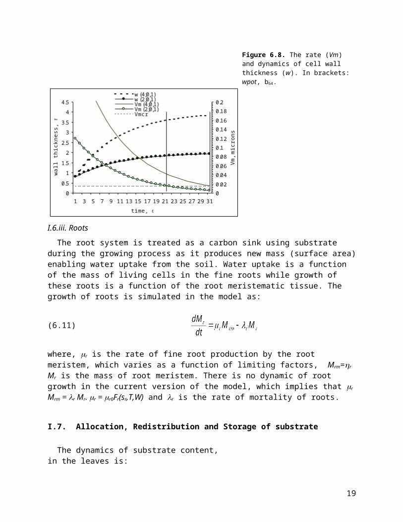
Wall synthesis irreversibly stops when Vm less then Vmcr (b62). Note that the equations for wall thickening are the same as those for enlargement. At optimal conditions wall synthesis is w=wpot-(wpot-wmin) EXP(-b64 t) (figure 6.8). The duration in the wall thickening stage, T, is T=1/b64 ln(b64(wpot-wmin)/Vmcr). As you can see on figure 6.8 the parameter b64=0.1, which was used in one version tuning, causes fast rates of wall thickening and the duration is only 30 and 22 days for cells with potential wall thickness 4 and 2 microns. With increasing value of b64 the rate of thickening is faster and duration during which cells remain in the thickening zone reduced. As in enlargement it is best to change Vmcr and b64 together to arrive at a reasonable time, for maximum wpot (figure 6.8).

Figure 6.7. The relationship of the potential cell wall thickness (wpot) on the cell size at different parameters. (in brackets: lmin, wmax, b63).

14

I.6.iii. Roots

The root system is treated as a carbon sink using substrate during the growing process as it produces new mass (surface area) enabling water uptake from the soil. Water uptake is a function of the mass of living cells in the fine roots while growth of these roots is a function of the root meristematic tissue. The growth of roots is simulated in the model as:

(6.11)

where, r is the rate of fine root production by the root meristem, which varies as a function of limiting factors, Mrm=r Mr is the mass of root meristem. There is no dynamic of root growth in the current version of the model, which implies that r Mrm = r Mr. r = r0Fr(sr,T,W) and r is the rate of mortality of roots.

I.7. Allocation, Redistribution and Storage of substrate

The dynamics of substrate content,in the leaves is:

(7.1)

in the stem is:

(7.2)

and in roots is:

(7.3)

Figure 6.8. The rate (Vm) and dynamics of cell wall thickness (w). In brackets: wpot, b64.

15

where, Sl, Ss and Sr are the substrate content [mM CO2] in the leaves, stem and roots respectively, likewise sl, ss and sr are substrate concentrations [mM CO2 kg-1] in the leaves, stem and roots, and ls and sr are coefficients of diffusion for the substrate from leaves to the stem and from the stem to the roots [kg t-1].

Daily allocation and redistribution subroutines control the relative distribution of sucrose among growth and storage at the leaves, stem and roots and usage by the three main sinks: respiration, growth and storage. Sucrose is assumed to be completely mobile throughout the tree each day, in accordance with studies that have shown that the distance of assimilate transfer is not a major factor limiting growth (Wardlaw, 1990), whereas stored starch is assumed to mobilize only when sucrose is fully depleted. Preferential use of sucrose is supported by studies with barley and sugar beet (Fondy and Geiger, 1982) that indicate starch mobilization in leaves at the beginning of the night was restricted until after sucrose in the leaves was reduced.

At the beginning of each day the cumulative amount of newly produced sucrose and any sucrose left from the previous day represents the new sucrose volume. Each sink and location is prioritized such that new photosynthate formed in the leaves is utilized in the following order:

1) Respiration in the a) leaves, b) stem, c) roots.

2) Growth in the d) leaves, Carbon allocation 'cascade'e) stem, f) roots.

3) Storage in the g) leaves, h) stem, i) roots.

Each day instantly available photosynthate 'trickles down' the carbon allocation cascade being depleted at each level by the amount of the specific sink, where Sink Strength = Sink Size Sink Activity (Taiz & Zeiger, 1991, p.171). The process continues until the sucrose is either completely utilized or the final sink (storage in the roots - i) is realized.

A percentage of the sucrose remaining at the end of the day will be allocated to starch. As a first approximation we assume a set daily rate of conversion from total sucrose to starch that is determined by the user (between 0 and 100%); for the data shown here this is 80%. It is realized that this rate will vary over time and among trees, and this may prove a key area of improvement in future model revisions. The relative proportions of sucrose that are converted to starch at each location within the tree (leaves, stem and roots) are determined by the relative volume of active cells in each location. This provides a link between reserve dynamics and growth activity, which is supported by observations on other tree species (Hansen 1967; Lacointe et al. 1993).

16

I.8. Soil water The content of water in soil of volume vs = Ash is calculated each day as:

(8.1) when w f

where, is the water content in soil volume vs [kg], is soil moisture [kg/ m3], Pr(t) is the precipitation [mm day-1], Pr(t)(1-a1 ) is the interception of precipitation by the crown (a1), Pr(t)a1

is the precipitation that goes into the soil. If Pr(t)a1 is greater than the value Pr*, there will be surface runoff equal to Pr(t)a1 - Pr

*. Additional loss of water occurs when the soil water content exceeds field capacity, and f . a2 is the rate of infiltration of water from the soil.

I.9. Isotope calculationsI.9.i. Carbon

I.9.i.a. Photosynthate Utilizing the model estimates for average daily concentration of CO2 inside the leaves (Ci), the basic equation of carbon isotope fractionation (13C) in C3 plants (Farquhar et al., 1982) has been used to model the 13C composition of photosynthate:

(9.1)

where, 13Cp is the 13C of photosynthate, 13Ca is the13C of ambient atmospheric CO2, (-4.4‰) is the maximum fractionation of 13C resulting from the diffusion of CO2 through leaf boundary air layers, ‰ is the maximum fractionation of 13C resulting from the biochemical reactions of carboxylation and PEP carboxylase (O’Leary, 1981), Ci is the leaf internal CO2 concentration, Ca is the ambient atmospheric CO2 concentration, and r is fractionation resulting from respiration (equations 9.2 and 9.3). Values of atmospheric CO2 concentration and 13C composition are estimated as annual values from ice core and flask measurements, where flask measurements are averaged for the summer months between May and October (Hemming et al., 1998). No account is presently taken of intra-annual variations in atmospheric CO2 concentration and 13C composition.

The diurnal respiration fluxes estimated for each site within the tree (leaves, stem and roots) (see section I.4), are used to estimate 13C fractionation from respiration at each site (r in equation 9.1). For the stem and roots it is assumed that the only form of respiration is dark respiration, which is modeled as follows:

(9.2)

17

where, 13Cdr is the 13C fractionation during dark respiration, ε is the maximum fractionation from dark respiration, Rd is the rate of dark respiration, κ is a complex parameter (refer to Farquhar et al., 1982) and Ca is ambient CO2 concentration.

For the leaves only, the 13C fractionations resulting from both dark and photo respiration are modeled using:

(9.3)

where, 13Cr is the 13C fractionation during dark and photo respiration, ρ is the maximum photo respiration fractionation and γ is the CO2 compensation point.

To translate the modeled photosynthate 13C compositions to 13C compositions for the whole leaf, stem and root daily estimates of carbon sink strength at each site and the source strength of presently formed photosynthate are used to determine the relative proportions of 13C contributed from presently formed photosynthate and remobilized starch. The 13C compositions of present photosynthate and stored starch in each location are estimated (see section I.7), and therefore an isotopic mass balance of present and stored photosynthate and starch can be used to estimate whole leaf, stem and root 13C composition:

(9.4)

where, Si and So are the carbon sink and source and the subscripts w, p and s indicate the whole sink area, photosynthate and starch respectively.

Daily estimates of sink strength and 13C composition for the stem are partitioned to specific cells within an annual ring using the model of cambial development (see section I.6), such that as each cell grows its 13C composition is modified by the 13C composition of the additional stem 13C. The final cell whole wood 13C composition therefore reflects the 13C compositions and proportions of the sources (photosynthate and starch) and the timing during which these sources are utilized in the formation of cell walls.

I.9.ii Oxygen and Hydrogen

The oxygen and hydrogen isotopic compositions (18O and D) of tree ring cellulose are modeled using the additional inputs of the 18O and D of precipitation and atmospheric water vapor. Three main steps are taken to translate these inputs to cellulose isotopic composition:

a. a basic soil water mixing model is used to mix the isotopic compositions of precipitation with existing soil water,

b. an established model is utilized to estimate evaporative enrichment in the leaf, and c. mixing factors are used to estimate the degree of mixing between waters in the leaf and

stem.

18

These steps are outlined below.

I .9.ii.a. Soil Water / Xylem Water

A basic soil-water mixing model is constructed to calculate daily values of 18O and D of soil water. With a precipitation event the 18O and D of the precipitation is combined with the isotopic compositions of the existing soil water in proportions comparable with the amounts of existing soil water (calculated per m2) and additional precipitation (figure 9.5), as follows:

(9.5)

Figure 9.5. Schematic of mixing model for soil water isotope composition.

where, VPREC and VSW are the volumes of precipitation falling on the soil area and of existing soil water, R is the radius of the horizontal extension of roots (of a circular “footprint” of roots centered on the tree bole), D is root depth, SW and SW-1 are the new isotopic composition (18O or D) of soil water and the estimation of soil water from the previous calculation step, and PREC is the isotopic composition of additional precipitation. The isotopic composition of soil water changes when soil water increases but does not change when it decreases. The existing parameter of maximum precipitation rate is utilized such that above the specified maximum precipitation rate water is lost to runoff and isotopic mixing in the soil does not occur.

At present, the soil water-mixing model contains no fractionation by evaporation in the surface soil layers and it is assumed that the water taken up by the roots is a representative sample of the whole soil water pool.

I .9.ii.b. Leaf Water Model

During uptake of soil water by roots and its translocation in the xylem to the leaves it is assumed that isotopic fractionations are insignificant. It is also assumed that, above the critical soil moisture threshold, the soil water of each day is available to the leaves the following day. Therefore, the xylem water entering the leaves on a specific day has 18O or D compositions equal to that of bulk soil water of the previous day.

The isotopic composition of leaf water at the sites of maximum evaporation (sub-stomatal cavities) is estimated using a basic model of water surface fractionation during evaporation

19

R = root radiusD

D

18OD

18O

VSW = soil water volume 18OSW DSW

D

18ODPREC

18OPREC

VPREC

R

(Craig and Gordon, 1965) adapted to include leaf boundary layers (Flanagan and Ehleringer, 1991):

(9.6)

where, LW is the 18O or D of leaf water, ' is the liquid-vapor isotopic fractionation factor (18O=1.0088, D=1.079), k is fractionation due to diffusion of H2O in air (18O =1.0285, D=1.025), XW is the 18O or D of xylem water, ei, eb, ea are vapor pressures of air at the leaf intercellular cavity, leaf boundary and ambient atmosphere, kb is fractionation due to diffusion of H2O through the leaf boundary layer (18O =1.0189, D=1.017), and RH is the 18O or D of atmospheric water vapor.

Equation 9.7 provides an option to mix the incoming xylem water with the isotopically enriched leaf water estimated in equation 9.2.

(9.7)

where, LWbulk is the 18O or D of bulk leaf water, LW is the 18O or D of leaf water calculated in equation 9.6, f is the fraction of bulk leaf water subjected to evaporative enrichment, and XW is the 18O or D of xylem water.

I .9.ii.c. Photosynthate and cellulose

Photosynthates that are formed in the chloroplast and cytosol of the leaves retain a component of the 18O and D compositions of the leaf water medium in which they were formed. However, autotrophic (dark) and heterotrophic (light) reactions may change these compositions significantly.

Assuming that the 18O and D compositions of bulk leaf water (estimated in equation 9.7) are representative of the leaf water medium in which photosynthates are formed, and that these compositions are subsequently modified by known autotrophic and heterotrophic fractionations, equations 9.8 and 9.9 are used to estimate photosynthate and cellulose 18O and D (non-exchangeable, carbon bound D only):

(9.8)

where, PS is the 18O or D of photosynthate exported from the leaves, LWbulk 18O or D of bulk leaf water and Eauto is autotrophic fractionation (27‰ for 18O (Sternberg & DeNiro, 1983),-171‰ for D (Yakir & DeNiro, 1990)) and Ehet is heterotrophic fractionation (0‰ for 18O, 158‰ for D (Yakir & DeNiro, 1990)).

(9.9)

20

where, C is the 18O or D (non-exchangeable) of cellulose, f is the fraction of H and O exchanged with xylem water (parameters isoH(3) and isoO(3)) and PS is the 18O or D of photosynthate (from equation 9.8).

EXTERNAL INPUTS

II.1. Daily Meteorological Data Daily meteorological data from Palisades Ranger Station meteorological station in the Santa Catalina Mountains near Tucson, Arizona (~4km from the study site - see section C.3.) were used as the fundamental inputs for the theoretical equations described above. The records of temperature (max and min) and precipitation from this station are available for the period 1965 to 1981. Linear regression relationships between these records and those from various meteorological stations within ~20km of this location were used to fill gaps and extend the records to cover ~100 years (1893/5 - 1999). The decision to use particular records or averages of various records for this reconstruction was made by correlating the various records available (and their averages) with the Palisades record, for the period 1965 to 1981. Those records with the highest correlations that cover the time period required for reconstruction were chosen. Gaps in each of the individual records were filled using regression relationships with the most highly correlated nearby record covering the required period.

The following sections detail the meteorological records and regression relationships used to construct the Palisades Ranger Station record for each parameter and without gaps.

II.1.i. Maximum Temperature

(in ºF , model converts to ºC)Actual data from Palisades: 1965-1981, includes gaps

Reconstructed data for Palisades: 1893-1964, 1982-1999, plus gaps in original recordRecords and regression relationships used for various time periods:Using Oracle record:

1893 - 1948: y = 0.9302x - 9.9979 R2 = 0.8975where x = Oracle max temperature.

Using Tucson Farm record (starts at 1949):1949-1964 and 1982-2000 plus gaps in Palisades record between 1965-1981:

y = 0.9458x - 15.236 R2 = 0.9231 where x = average of Oracle and Tucson Farm max temperature.

Gaps in the Oracle record:For the periods 1894-1964 and 1982-1999 gaps in the Oracle record were filled using the U of A record and the following regression relationship:

21

y = 0.9451x - 4.3646 R2 = 0.9251 where x = U of A max temperature

For the period 1965-1981 gaps in the Oracle record were filled using the Sabino Canyon record and the following regression relationship:

y = 0.9359x - 3.5625 R2 = 0.9412where x = Sabino Canyon max temperature

The following gaps (days in year) existed in both the U of A and Oracle records prior to 1949 so were filled with linear interpolation between the two adjoining data points:

1893 69-72, 104-112, 119-122, 167-172, 227-2321894 11-16, 29-36, 105-107, 1771900 601911 3181915 318-3261920 276-2801928 182-1851936 279-2801938 320

Gaps in Tucson Farm record: For the period 1949-1982 gaps in the Tucson Farm record were filled using the Sabino Canyon record and the following regression relationship:

y = 0.9656x + 2.5678 R2 = 0.9796 where x = Sabino Canyon max temperature

For the period 1982-1999 gaps in the Tucson Farm record were filled using the U of A record and the following regression relationship:

y = 0.9728x + 1.9367 R2 = 0.9611 where x = U of A max temperature

II.1.ii. Minimum Temperature

(in ºF , model converts to ºC)Actual data from Palisades: 1965-1981, includes gaps

Reconstructed data for Palisades: 1893-1964, 1982-1999, plus gaps in original recordRecords and regression relationships used for various time periods:

Using average of U of A and Oracle averaged record:1893 - 1964 and 1982-1999 plus gaps in Palisades record between 1965-1981:

y = 0.8503x - 7.1634 R2 = 0.8588 where x = Average of U of A and Oracle min temperature.

Gaps in the U of A record:For the period 1893 - 1949 gaps in U of A record were filled using the Oracle record and the following regression relationship:

22

y = 0.9463x + 8.6709 R2 = 0.787 where x = Oracle min temperature.

For the period 1949 - 1999 gaps in U of A record filled using the Tucson Farm record and the following regression relationship:

y = 0.9032x + 10.814 R2 = 0.9238 where x = Tucson Farm min temperature.

The following gaps (days in year) existed in both the U of A and Oracle records, these were filled with linear interpolation between the two adjoining data points:

1893 69-72, 104-112, 119-122, 167-172, 227-2321894 11-16, 32-39, 105-107, 1771897 1891900 601911 3161912 1861915 316-3241920 274-2781928 180-1831929 3471936 277-2781975 1051963 202

Gaps in the Oracle record:For the period 1894 - 1999 gaps in Oracle record filled using the following regression relationship:

y = 0.8316x + 3.374 R2 = 0.787 where x = U of A min temperature.

II.1.iii. Precipitation

All precipitation reconstructions are based on regression equations forced through the origin. Winter (Jan-Apr, Nov-Dec) and Summer (May-Oct) periods were separated to facilitate better reconstructions.

Actual data from Palisades: 1965-1981, includes gapsReconstructed data for Palisades: 1895-1964, 1982-1999, plus gaps in original record.Records and regression relationships used for various time periods:

WINTER (Jan-Apr, Nov-Dec)Using average of U of A and Oracle averaged record:

1895 - 1948: y = 1.316166x R2 = 0.3963 where x = U of A and Oracle average winter precipitation

Using Sabino Canyon record:1949 - 1964 and 1981 - 1982 and gaps in Palisades record:

23

y = 1.776523x R2 = 0.5909 where x = Sabino Canyon winter precipitation

Using Cascabel record:1983 - 2000:

y = 2.4346x R2 = 0.591 where x = Cascabel winter precipitation

Gaps in U of A record:For the period 1895 - 1948 gaps in the U of A record were filled using the Oracle record and the following regression relationship:

y = 0.2667x R2 = 0.1448 where x = Oracle winter precipitation

For the period 1949 - 1999 gaps in the U of A record were filled using the Tucson Farm record and the following regression relationship:

y = 0.643x R2 = 0.3633 where x = Tucson Farm winter precipitation

Gaps in Oracle record:For the period 1895 - 1999 gaps in the Oracle record were filled using the U of A record and the following regression relationship:

y = 0.691x R2 = 0.1282 where x = U of A winter precipitation

Gaps in Sabino Canyon record:For the periods 1949 - 1964 and 1981 - 1982 gaps in the Sabino Canyon record were filled using the Tucson Farm record and the following regression relationship:

y = 0.9951x R2 = 0.7771 where x = Tucson Farm winter precipitation

SUMMER (May - October)Using U of A and Oracle averaged record:

1895 - 1960: y = 1.084108x R2 = 0.267where x = U of A and Oracle average summer precipitation

Using U of A, Oracle, San Manuel, Kitt Peak and Tucson Airport averaged record:1961 - 1964 and 1981 - 1999 and gaps in Palisades record:

y = 1.391374x R2 = 0.3609 where x = Average of U of A, Oracle, Kitt Peak, San Manuel,

Tucson Airport.

Gaps in the U of A record:For the period 1895 - 1948 gaps in the U of A record were filled using the Oracle record and the following regression relationship:

y = 0.2667x R2 = 0.1448 where x = Oracle summer precipitation

24

For the period 1949 - 1999 gaps in the U of A record were filled using the Tucson Farm record and the following regression relationship:

y = 0.643x R2 = 0.3633 where x = Tucson Farm summer precipitation

Gaps in the Oracle record:For the period 1895 - 1999 gaps in the Oracle record were filled using the U of A record and the following regression relationship:

y = 0.691x R2 = 0.1282 where x = U of A summer precipitation

Gaps in the Kitt Peak record:For the period 1961 - 1999 gaps in the Kitt Peak record were filled using the Tucson Farm record and the following regression relationship:

y = 0.8306x R2 =0.142 where x = Tucson Farm summer precipitation

Gaps in the San Manuel record:For the period 1955 - 1999 gaps in the San Manuel record were filled using the Tucson Farm record and the following regression relationship:

y = 0.5184x R2 = 0.2066 where x = Tucson Farm summer precipitation

Gaps in the Tucson Airport record:For the period 1948 - 1999 gaps in the Tucson Airport record were filled using the U of A record and the following regression relationship:

y = 0.5926x R2 = 0.3654 where x = U of A summer precipitation

II.1.iv. Dew Point Temperature

(in ºC)Actual data from Palisades: 1st April 1997 - 31st Dec 1997, includes gaps

Reconstructed data for Palisades: 1st October 1948 - 30th June 1998, plus gaps in original record. Records and regression relationships used for various time periods:Using Tucson Airport record:

1948 - 1964 and 1984 - 1998: y = 0.8836x - 5.9552 R2 = 0.7952where x = Dew point temperature (ºC) at Tucson Airport

Gaps in the Tucson Airport record:For the period 1965 - 1983 gaps in the Tucson Airport record were filled using the Tucson Airport 700hPa upper air record and the following regression relationship:

25

y = 0.0742x + 4.2468 R2 = 0.617where, x = Dew point temperature at 700hPa (ºF) at Tucson Airportnote: y = Reconstructed Tucson Airport dew point temperature in ºC

Other gaps in the Tucson Airport record:For the period 1948 - 1998 remaining gaps in the Tucson Airport record were filled by linear interpolation between the two adjoining data points.

II.2. Isotope InputsII.2.i. 13C of atmospheric CO2

Annual values of atmospheric 13C are estimated from ice core and flask measurements (figure II.1). The values are changed on January 1st each year. No allowance is presently made for intra-annual changes in CO2.

Figure. II.1. Atmospheric CO2 concentration (circles) and carbon isotope (13C) composition (triangles). CO2 concentration data is from the Siple ice-core, Antarctica; filled circles, 1899 - 1953 (Friedli et al., 1986), South Pole summer average (April - September) air flask measurements; filled circles, 1957 - 1988 (Keeling and Whorf, 1996) and Schauinsland, Germany summer average air flask measurements; open circles 1972 - 1992. 13C data is from the Siple ice core; filled triangles, 1895 - 1953 (Friedli et al., 1986), Vermunt, Austria summer average (April - September) air flask measurements; filled triangles, 1966 - 1974 (Levin et al., 1994), Schauinsland summer average air flask measurements and filled triangles, 1977 - 1992 (Levin et al., 1994). A 6th order polynomial fitted to the 13C data (excluding the eastern England measurements) is assumed to be the general atmospheric 13C trend over the last 100 years.

II.2.ii. 18O and D of precipitation and atmospheric water vapor

Measurements of the 18O and D of precipitation collected at a site in Tucson from January 1982 (Long, unpublished data) are used as initial inputs for the soil water model. The following methods are used to fill gaps that exist in these records. Where values are not available, but a precipitation event has occurred at the site, a regression model between 18O of precipitation and

26

average daily temperature for the same site in Tucson is used to estimate 18O of precipitation (figure II.2).

Figure II.2. Regression model used to fill gaps in 18O of precipitation data

Where the 18O of atmospheric vapor is not available it is estimated from a regression model (18Ovap(i)=(0.4002*18Oprec(i))-13.627) between 18O of atmospheric vapor and 18O of precipitation (figure II.3).

Figure II.3. Regression relationship of 18O of vapor and 18O of precipitation at Tucson. Regression model is used to fill gaps in the 18O of vapor series.

27

Where data is not available the D of precipitation and vapor was calculated from a regression model between 18O of precipitation/vapor and D of precipitation/vapor (figure II.4).

Figure II.4. Regression relationship of 18O and D (versus VSMOW) in precipitation at Tucson, Arizona, USA. This regression model is used to fill gaps in the D of precipitation and vapor series.

II.3. Allometric DataII.3.i. Tree age:height:radius curve

The existing TreeRing model (Fritts et al, 1999) assumed that height growth, crown growth, root growth and soil volume were constants. However in applications to younger trees it was necessary to simulate the yearly increase in height, crown, stem, roots and soil volume for the growing tree. We therefore collected field measurements of tree diameter at breast height (dbh is 1.3 m) and tree height from 21 trees in the study area. In addition, we examined the existing cores from these trees and recorded the pith year (dbh), the first year in which the cell size and wall thickness measurements began, the distance in mm between them, heartwood width and sapwood width. Some cores did not reach the pith so in these cases a template of concentric circles was used to estimate the number of years and distance to the center using the curvature of the innermost rings in the core.

These measurements were entered into a Microsoft Excel spreadsheet and equations were developed for estimating the heartwood radius from the total radius of the stem and total tree height from the age of the tree (Figures II.5 and II.6).

28

vapor

precipitation

Figure II.5. The equation used to estimate heartwood radius from the total radius of the tree stem derived from observations on the study area trees.

Figure II.6. The equation used to estimate height from tree age derived from

29

observations on the study area trees.

The necessary data to estimate stem height growth, crown mass and other related parameters were entered into file Trg70.i0. The subroutine Trginput.for was rewritten to read these data and to calculate the following:

1. The age and radius (rt) of the ring prior to the beginning of existing independent measurements were calculated from the pith date and radius measurement. If the simulation did not begin with the first available measurement, the measurement file with a .CRN extent is opened, and the ring width measurements are read from this file up to the starting date of the simulation.

2. A young tree was harvested and the needle traces were used to determine the number of needles produced in each internode year from 1962 to 1998 and the length of the internode was measured (Hemming et al. 2001). The number of needles formed each year was converted to an index by dividing each number by the average. A multiple regression estimated the needle number index from monthly temperature and precipitation of current and prior year. The coefficients from the regression were entered as parameter zini(51-99) (Table 4) with all zero coefficients entered as blank fields. Subroutine TRGINPUT.FOR calculates the estimated needle number index using the monthly climatic data from the current and previous year. During the first year where the prior year climatic information is not available the index is assigned a value of 1.0

3. Stem area at breast height is then calculated from the current radius.

4. The maximum depth and area of the soil are read from p(14) and p(15). However, zini(37) is a Michaelis-Menten constant age*. If its value is greater than zero, depth is calculated as a function of age: depthI =age/(age +age*) * p(14). The soil area is estimated later as a fractional percent of crown area (zini(29)) if zini(29) is greater than zero.

5. Height (h) is calculated as a function of age using zini(18) and zini(19): h = -0.0002 age2 +0.1605 age (Fig. 6). The maximum height is calculated from the maximum age using the same parameters

6. The surface (s) of the cambium in the stem and root is estimated from the surface of an open-top cylinder as s = 2 pi * radius (tree height + depth of roots).

7. Heartwood radius is estimated from the total radius as observed on cores extracted from the study site trees: rh = 0.5666rt – 36.411. If the estimated rh is less than 0, rh is set to zero (figure II.5). The heartwood area in cm2 and m2 is then calculated.

8. Sapwood radius () and area are calculated by subtracting the heartwood radius.

9. The crown mass for Pinus ponderosa is calculated from the sapwood area and product of crown ratio and crown length using the allometric equations of Monserud & Marshall (1999). The crown ratio and length were measured from the study area trees.

10. Crown area is estimated as a function of crown mass by multiplication of the mass with p(3), the coefficient of conversion of leaf mass to area. This parameter is obtained using fresh 5-needle clusters sampled from the study area trees. Area is estimated from the length and width of the fresh needles and divided by their dry weight.

30

11. The soil area available to precipitation is estimated as a fractional percent of crown area (zini(29)).

12. The phloem area and volume are estimated as a cylinder surrounding the stem volume estimate using phloem thickness (zini(13)) obtained from the study area trees.

13. The circumference of the cambium and the number of tracheid initials are estimated from the tangential size of the initials (pp(28)) and the fractional percent of rays (zini(24)). Cambial area (S) is the surface of the estimated cylinder surrounding the stem.

14. The volume of coarse roots is estimated from the stem area at the soil surface and depth of roots. The density of root wood is assumed to be the same as density of stem wood (den(3)).

15. A special set of coefficients is calculated for use in the estimation of respiration. Coefficients K, Sapwood volume (V) and N are calculated as: K = delta ((1-delta) /2/rt), V = K*S and N = 2*pi*rt, where delta is the sapwood radius, rt is the radius of the stem wood and S is the surface area of the cambium.

16. Sapwood mass is calculated from sapwood V*den(2) and phloem mass from phloem volume*den(2).

17. Fine root mass is estimated as a proportion of the other masses: Rmass = zini(39)*crown mass*sapwood mass*phloem mass.

18. In the first year the mass of the current and previous summer foliage is calculated as ½ of the total mass. In subsequent years the mass of the second year needles is subtracted from the total foliage mass to obtain the current year’s needle mass.

19. The current year uncorrected needle mass is multiplied by the needle index to account for the effects of climate on needle growth.

Subroutine TRGINPUT.FOR is called once at the beginning of the first year to calculate the initial value of these variables and then again on day p(51) to calculate the needle growth of the current year and all other input variables. It is then called on day p(51) in each subsequent year.

In normal mode, when op(20) is zero, these calls on day p(51) use the dendrograph estimate of growth in the current year to estimate the new stem radius and all the calculations are made using this datum. However, in the subsequent year the true estimated ring width of the previous year replaces this estimate and the current growth, estimated from the dendrograph estimate, is added to estimate the stem radius.

There is a second mode, when op(20) is 1, in which the calls on day p(51) use the actual ring widths rather than the estimated value. This allows the model to track any anomalous growth patterns in the simulated tree. This option has not been used extensively and is not well tested at present. Normal mode is used in subsequent discussions.

The array, hold, passes the following values to the main program:

1. Hold(1): Current radius m

2. Hold(2): Empty

3. Hold(3): Empty

4. Hold(4): Sapwood mass kg

31

5. Hold(5): Fine root mass kg

6. Hold(6): Height in m

7. Hold(7): Not used

8. Hold(8): Sapwood Volume (V)

9. Hold(9): K which becomes variable form in the main program.

10. Hold(10): Volume of living stem cells

11. Hold(11): Mass of 1-year-old needles kg

12. Hold(11): Mass of 2-year-old needles kg

13. Hold(12-20) Needle mass for trees holding up to 10-year-old needles.

A total of 29 input variables are written to file “*I.DAT” along with the contents of the arrays “Hold” and “Zini” from Trg70.i0.

II.3.ii. Relationship between volume and mass of sapwood and the volume of live cells in the sapwood.

The sapwood volume, V, is:

(1) V= (2R-)h

The sapwood surface area, S, is:(2) S=2Rh

The relationship between the sapwood volume and the surface area of sapwood is:

(3) V=(1-/2R)S,or V=kS, where, k=(1-/2R).

The number of cellular files, N, is calculated as:

(4) N=2R/dtang,

where, dtang is the tangential cell size of the initial cell.

If cell wall area is denoted by a then the cell wall volume, Vw, of for “long” cells (where length is equal the height, h, of the tree) is:

(5) Vw=ahN

or by rewriting equations 2 and 3:

(6) Vw=ah2R/dtang=a/dtangS=a/dtang V/k

32

h

RSapwood radius

Equation 6 is used for calculation of the cell wall mass dynamic. Cell wall mass is:(7) M=Vwwhere, is the density of wall in mMCO2/m3.

The density of wall is assumed to be 1300 kg/m3 or 1.3-12 g/micron3 (Silkin, 2001). Assimilated CO2 is converted to dry matter equivalents by multiplying by 28.5 g mol-1 (Landsber,1986 p89). Dry weight is then converted to mMCO2 units by multiplying by 1/28.5=35.09 mMCO2 g-1. Therefore, for additional cell wall area and volume growth we used the coefficient 45.617 mMCO2 /micron3 (1.3-12 x 35.09).

33

II.4. Parameters

Table 1. Filename ‘TRG70.PAR’, parameters (p) for main TreeRing program (TRG70.FOR)

2.0 1  Maximum age of foliage yr20.0 2 halfRadRadiation at which photosynthesis reaches 1/2 maximum Wm-2

7.0 3  Coefficient of conversion of leaf mass to area m2kg-1

250.0 4 RminMinimum resistance to diffusion of water sm-1

550.0 5 RmaxMaximum resistance to diffusion of water sm-1100-1

6    -5.0 7 CtPeriod for averaging leaf growth for threshold rate Days0.01 8 CtsCritical threshold average rate to stop crown growth  0.01 9 sm1Wilting point vv-1

0.109 10 sm2Optimal soil moisture vv-1

0.23 11 sm3Maximum optimal soil moisture vv-1

0.25 12 sm4Maximum moisture at which water absorption stops vv-1

0.24 13 sm5Field capacity vv-1

0.6754 14 hMaximum depth of the tree root system m30.0 15 SareaMaximum soil surface area, actual estimated from age or height m2

0.89 16 K6Coefficient of available precipitation 1Day-1

100.0 17 APMaximum available precipitation mm0.5216 18 K1Water absorption per unit of root kgdm-3h-1

1.65 19 K3Coefficient for diffusion of CO2 relative to water  0.45 20  Carbon concentration of wood kgC-1kg dry wt-1

-10.0 21 TminMinimum day temperature for photosynthesis Celsius9.57 22 Topt1Optimal temperature for photosynthesis Celsius23.0 23 Topt2Maximum optimal temperature for net photosynthesis Celsius40.0 24 TmaxTmax - Maximum temp when net photosyn. becomes 0 Celsius

12.5 25 CO2aCO2 concentration in the air mMm-3

1.5 26 AMinimum CO2i (photosynthetic compensation point) mMm-3

10.5 27 BMaximum (saturation) concentration of CO2i mMm-3

0.419 28 CTRelative crown growth rate threshold to form latewood  0.38 29 CtmCrown growth threshold to begin cell wall thickening  

120.0 30  Maximum average resistance to prevent growth beginning  20.0 31  Period to calculate temperature sum Days

120.0 32 sumtTemperature sum to begin growth Celsius0.0 33  Days after Critical Day Length that growth can begin 0.0 Days

10.0 34  Michaelis-Menthon coefficient of maintnance respiration  -5.7 35 astminMinimum temperature for leaves Celsius10.1 36 astopt1Optimal temperature for leaves Celsius22.1 37 astopt2Maximum optimal temperature for leaves Celsius30.1 38 astmaxMaximum temperature where leaf growth becomes 0 Celsius

39     0.0 40 r1Diffusion of water from soil below field capacity  

0.072 41  Minimum water concentration in the stem vv-1

0.72 42  Maximum water concentration in the stem vv-1

2.0 43  Hourly rate of water absorption from stem kgdm-3h-1

0.08 44  Hourly rate of stem water recharge from soil kgdm-3h-1

1.0 45  Scale for active radius   46    

11.0 47  Sensitivity of leaf growth to resistance: full(10), low (1)  10.0 48  Sensitivity of root growth to resistance: full(10), low (1)  

0.555 49  Fractional percent leaf surface exposed to light  12.5 50  Day length to begin growth Hours

244.0 51  Day number to calculate new needle mass Day28.0 52  Number of days of transition to new needle mass Days

53      54      55     

0.03 56 PmaxMaximum rate of photosynthesis mMm-2s-1

0.0 57     4.0 58  Difference needed to begin averaging for earlywood-latewood  

188.0 59  Day number to begin checking for earlywood-latewood boundary  4.0 60  Number of days to average for earlywood-latewood boundary  

    Density parameters1200.0 1 den(1)Density of xylem cell wall kgm-3

360.0 2 den(2)Density of phloem, rays (balsa wood) kgm-3

459.0 3 den(3)Density of Ponderosa pine wood (Carey et al, 1966) kgm-3

4      5         Maintenance respiration

180.0 1 rmc(1)Coefficient for foliage @t=10ºC (Ryan, 1995) mMCO2m-3day-1

100.0 2 rmc(2)Coefficient for living stem tissues @t=10ºC (Ryan, 1995) mMCO2m-3day-1

160.0 3 rmc(3)Coefficient for roots @t=15ºC (Ryan, 1995) mMCO2m-3day-1

0.069 1 rmt(1)Temperature coefficient for foliage 1/0 deg.C0.069 2 rmt(2)Temperature coefficient for living stem tissues 1/0 deg.C0.069 3 rmt(3)Temperature coefficient for roots 1/0 deg.C

    Carbon use efficiency in growth respiration of…

0.785 1 grc(1) Leaves/crown mMCO2kg-1day-1

2 grc(2)    3 grc(3)    4 grc(4)   

0.8 5 grc(5)Roots mMCO2kg-1day-1

    Coefficients in Michaelis Menton equation for concentration of sucrose when 1/2 maximum rate 15000.0 1 gc(1)Michaelis Menton constant for leaves when 1/2 maximum rate mM1000.0 2 gc(2)Concentration of sucrose when leaf growth stops mM

3 gc(3)   525.0 4 gc(4)Concentration of sucrose when root growth stops mM798.5 5 gc(5)Michaelis Menton constant for roots when 1/2 maximum rate mM

    Proportion of growing tissue of living mass in…0.012 1 prp(2)Leaves  

12

0.0 2 prp(1)Cambial area, calculated by TRGINPUT program if 0  0.023 3 prp(3)Roots  

    Maximum growth rate of…1.67 1 upt(1)Leaves (increase to shorten season) 1/day

0.0494 2 upt(2)Roots  0.0 3 upt(3)   0.0 4 upt(4)   0.0 5 upt(5)   

    Beginning threshold for Resistance Limitation to begin (250 Min)40000.0 1 xrmn(1)Leaves  40000.0 2 xrmn(2)Roots  

3 xrmn(3)    4 xrmn(4)   5 xrmn(5)      Max Resistance when growth stops (55000 Max)55000.0 1 xrmx(1)Leaves  55000.0 2 xrmx(2)Roots  

3 xrmx(3)    4 xrmx(4)    5 xrmx(5)   

13

Table 2. Filename ‘CAMB70.PAR’, parameters (b) for CAMBIUM subroutine (camb70.for)

16.3 1  Minimum cell size  49.0 2  Maximum cell size  30.0 3  Tangential cell size  2.0 4  Minimum cell wall thickness  

15.0 5 AmaxMaximum cell wall area  0.18 6  Minimum of lumen area (fractional percent)  2.0 7  Minimum cell wall thickness  

8      9     

7.9 10  Size of dividing cell between G1 & S (Chromosomes begin to replicate)9.0 11  Size of dividing cell between S & G2 (Division begins)  9.5 12  Size dividing cell between G2 & M (Mitosis begins)  

10.0 13  Size of dividing cell when it begins to divide   14      15      16      17      18      19     

50.0 20  Maximum number of cells in any cambial zone    Control of cambial division 

0.01 21  Minimum growth rate below which the cambium is dormant  0.32 22  Scalar of growth rate  0.16 23  Growth rate during S, G2 and M phases of the cell cycle  

0.225586 24 KmaxMaxmum slope of division rate  10.0398 25 VpDivision rate at 60mKm assumed when few cells present  

0.06 26  Coefficient b3 (Vmin) equation 6.5. Curve to switch to enlargement  32.55 27  b2(Vmin) equation 6.5. Switch to enl. curve (Increase to incr. enl. time)  

17.3281 28  Distance of growing cells when slope of division rate is 1/2 maximum microns12.4 29  Day length to stop cambial and leaf growth hours

-10.0 30  Period to average Ct  1.0752 31  Sensitivity of division to Ct (1 is minimum - 10 is maximum)  

5.5 32  Sensitivity of vmin in Cambium to Ct (1 is maximum - 10 is minimum)20400.0 33  Minimum sugar concentration when division stops mK

235430.0 34  Michaelis Menton coefficient for sugar limitation to division mK10000.0 35  Maximum resistance for division to occur, division stops <55000  

400.0 36  Minimum resistance to division limitation, limitation begins >250  -5.0 37  Minimum temperature for division  10.0 38  Optimal temperature for division  23.0 39  Maximum optimal temperature for division  40.0 40  Maximum temperature where division becomes 0  10.0 41  Sensitivity of division to resistance (10 is maximum - 1 is minimum)  

    Control of enlargement0.1 42 VcreCritical rate when enlargement switches to maturation micronsDay-1

43     0.0169 44  Potential from distance  

9.5 45  Minimum distance  

14

0.4 46  Rate of enlargement micronsDay-1

47      48     

4.0 49  Sensitivity of enlargement to resistance (10 is maximum - 1 is minimum)  -5.0 50  Period of average for control of enlargement Days2.0 51  Sensitivity of enlargement to Ct (10 is maximum - 1 is minimum)  

52     40000.0 53  Minimum sugar concentration when enlargement stops mK22900.0 54  Michaelis Menton coefficient in equation of growth control by sucrose mK55000.0 55  Maximum resistance for enlargement to occur, enlargement stops <55000  

350.0 56  Minimum resistance to enlargement limitation, limitation begins >250  -5.0 57  Minimum temperature for enlargement to occur ºC7.0 58  Optimal temperature for enlargement rate ºC

25.5 59  Maximum optimal temperature for enlargement rate ºC30.0 60  Maximum temperature where enlargement becomes ºC

    Control of maturation 61    

0.0 62 VcrmCritical rate to stop thickening mKmDay-1

0.2 63  Cell size control of thickening rate  0.2 64  Rate of thickening  

65      66      67      68     

10.0 69  Sensitivity of maturation to resistance (10 is maximum - 1 is minimum)  -2.0 70  Period of average for control of maturation Days10.0 71  Sensitivity of maturation to Ctm (10 is maximum - 1 is minimum)  

72     30000.0 73  Minimum sugar concentration when maturation stops mK23437.5 74  Michaelis Menton coefficient in equation of control growth by sucrose  10000.0 75  Maximum resistance for maturation to occur, maturation stops <55000  2050.0 76  Minimum resistance for maturation to occur, limitation begins >Rmin  

-5.0 77  Minimum temperature for wall thickening ºC14.0 78  First optimal temperature for wall thickening ºC28.5 79  Second optimal temperature for wall thickening ºC35.0 80  Maximum temperature for wall thickening ºC

    Control of respiration25.0 81  Coefficient of maintenance respiration for stem cells b1  

0.0868 82  Temperature coefficient of maintenance respiration   83  R10, respiration at 10ºC   84      85      86      87      88      89     

0.8 90  Efficiency of division growth mMCO2cell-1day-1

0.8 91  Efficiency of enlargement growth mMCO2cell-1day-1

0.8 92  Efficiency of maturation growth mMCO2cell-1day-1

15

93      94      95      96      97      98      99     

0.0 100  Use only living cells for distance (0), Use all cells for distance (1)  

16

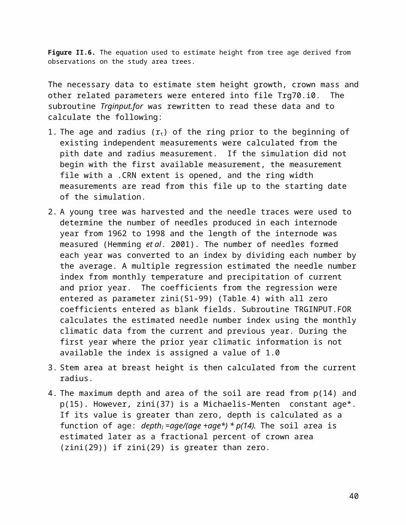
Table 3. Filename ‘ISO.PAR’, for ISOTOPE subroutine (isotope.for).

  Common parameters for isotope calculations (isoAll(i)) 0.7 1  Leaf surface vapor pressure (vp) as proportion of external - internal vp's  

22.4 2  Volume of one mole of an ideal gas at STP ( T=0ºC and P=101300Pa)  273.15 3  Zero degrees Kelvin ºK

1.0 4  Portion of sucrose allocated to storage each day, 0.0=0%, 1.0=100%  1.0 5  Maintenance respiration before growth in leaf? 1.0=yes, 2.0=no  1.0 6  Maintenance respiration before growth in stem? 1.0=yes, 2.0=no  1.0 7  Maintenance respiration before growth in root? 1.0=yes, 2.0=no  

  8       9      10      11      12      13      14      15     

  Carbon isotope parameters (isoC(i)) -4.4 1  Maximum fractionation from diffusion of CO2 into leaf  -30 2  Maximum fractionation from carboxylation  

3 3  Discrimination against 13C during photorespiration  1.5 4  Discrimination against 13C during dark respiration  10 5  Difference in altitude between trees and met. station (minus=met lower) m

6     148 7  CO2 compensation point mMCO2

0.245 8  Carboxylation efficiency (k in the Farquhar equation)   9      10      11      12      13      14      15     

  Oxygen isotope parameters (isoO(i))   1     

1 2  Proportion of Craig-Gordon leaf water in bulk leaf water  0.12 3  Proportion of carbon-bound oxygen in cellulose from xylem water  

1.137 4  Majoube (1971) water-vapor 'a' term in equation of T Vs 18Ol-v  -0.4156 5  Majoube (1971) water-vapor 'b' term in equation of T Vs 18Ol-v  -2.0667 6  Majoube (1971) water-vapor 'c' term in equation of T Vs 18Ol-v  

0.002005 7  18O:16O for reference material - VSMOW  1.0285 8  Craig-Gordon model kinetic diffusion (kd) fractionation into stomatal pore (Merlivat 1978)1.0189 9  Craig-Gordon model, kd fractionation in boundary layer (Flanagan & Ehleringer 1991)

27 10  Biochemical fractionation during carbohydrate synthesis  0.1351 11  Regression slope coefficient for average daily temperature to 18O precipitation relationship

-13.028 12  Regression intercept for average daily temperature to 18O precipitation relationship

17

-3.28 13  18O altitude effect from UofA to Palisades (1640m alt difference)  0.4002 14  Regression slope coefficient for 18O precip. to 18O vapor relationship  

-13.627 15  Regression intercept for 18O precip. to 18O vapor relationship    Hydrogen isotope parameters (isoH(i)) 

1     1 2  Proportion of Craig-Gordon leaf water in bulk leaf water  

0.42 3  Proportion of carbon-bound hydrogen in cellulose from xylem water  24.844 4  Majoube (1971) water-vapor 'a' term in equation of T Vs Dl-v  

-76.248 5  Majoube (1971) water-vapor 'b' term in equation of T Vs Dl-v  52.612 6  Majoube (1971) water-vapor 'c' term in equation of T Vs Dl-v  

0.000156 7  D:H for reference material - VSMOW  1.025 8  Craig-Gordon model, kd fractionation through stomatal pore (Merlivat 1978)1.017 9  Craig-Gordon model, kd fractionation in boundary layer (Flanagan & Ehleringer 1991)-171 10  Autotrophic biochemical fractionation during carbohydrate synthesis (Yakir & DeNiro 1990)158 11  Heterotrophic biochemical fractionation during carbohydrate synthesis (Yakir & DeNiro 1990)

6.6149 12  Regression slope coefficient for 18O precip to D precip and vapor relationship-2.4751 13  Regression intercept for 18O precip to D precip and vapor relationship  

  14       15     

18

Table 4. Filename ‘TRG70.IO’, initial input parameters.

Initial input parameters, zini(i)0.0 1  Initial stem water

  2       3     

-15.0 4dDstL Hydrogn isotope composition (D) of initial starch in the leaves ‰VSMOW-15.0 5dDstS D of initial starch in the stem ‰VSMOW-15.0 6dDstR D of initial starch in the roots ‰VSMOW

35.0 7d18stL Oxygen isotope composition (18O) of initial starch in the leaves ‰VSMOW

35.0 8d18stS 18O of initial starch in the stem ‰VSMOW

35.0 9d18stR 18O of initial starch in the roots ‰VSMOW

-22.0 10d13CstL Carbon isotope composition (13C) of initial starch in the leaves ‰VPDB

-22.0 11d13CstS 13C of initial starch in the stem ‰VPDB

-22.0 12d13CstR 13C of initial starch in the roots ‰VPDB0.0 13  Thickness of phloem m0.2 14  Initial soil moisture vv-1

2500.0 15  Initial photosynthate in the crown mM20000.0 16  Initial photosynthate in the stem mM2000.0 17  Initial photosynthate in the root mM

-0.0002 18  Height equation coefficient for age2 m0.1605 19  Height equation coefficient for age m0.5666 20  Heartwood area coefficient for age2 cm2

-36.411 21  Heartwood area coefficient for age cm2

22     23    

0.1 24  Fractional % rays / unit length of cambium mm-1

0.0207 25  B0 Coefficient (from Monserud and Marshall, 1999)  0.6903 26  B1 Exponent sapwood area / crown mass cm2kg-1

0.9543 27  B4 Exponent crown length m0.44 28  Fractional % crown height / total tree height mm-1

0.4 29  Fractional % soil surface area / leaf area m2m-2

1919 30  Pith Date y1940 31  First measured year date y0.032 32  Distance from first measured year to pith m

33     34      35     36    

40 37  Age at which depth will be 50% of maximum depth  0.00015 38  Average radial diameter of cambial cells m

0.03 39  Fine Root/Remaining Shoot, mass (dry weight) kgkg-1

  40       41       42       43     

19

  44       45       46       47       48       49       50     

  Regression Coefficients for Needle Number Index   51  Previous January Temperature ºF  52  Previous February Temperature ºF  53  Previous March Temperature ºF  54  Previous April ºF

0.04429 55  Previous May ºF  56  Previous June ºF  57  Previous July ºF  58  Previous August ºF0.017221 59  Previous September ºF

60  Previous October ºF-0.03053 61  Previous November ºF

62  Previous December ºF 63  Current January Temperature ºF 64  Current February ºF0.038246 65  Current March ºF

66  Current April ºF 67  Current May ºF 68  Current June ºF 69  Current July ºF 70  Current August ºF 71  Current September ºF 72  Current October ºF 73  Current November ºF 74  Current December ºF 75  Previous January Precipitation Inches 76  Previous February Precipitation Inches

0.03391 77  Previous March Inches 78  Previous April Inches 79  Previous May Inches 80  Previous June Inches0.033955 81  Previous July Inches-0.01793 82  Previous August Inches-0.02765 83  Previous September Inches

84  Previous October Inches-0.0237 85  Previous November Inches

86  Previous December Inches0.01462 87  Current January Precipitation Inches

0.021297 88  Current February Precipitation Inches0.042747 89  Current March Inches

90  Current April Inches 91  Current May Inches 92  Current June Inches

20

93  Current July Inches 94  Current August Inches 95  Current September Inches 96  Current October Inches 97  Current November Inches 98  Current December Inches

-3.72193 99  Regression constant    100     

21

Table 5. Filename ‘TRG70.INF’, control parameters (TRG) for TreeRing program

(A1)Filter temp data (see note 1)d:\data\model\ (A40) Path for climatic dataPali1940 (A8) File name of climatic datacatalstd.crn (A12) Indexed Chronology Named:\data\model\ (A40) Path to cell and index dat.cata04Nt (A8) Files CRN - size & thicknessCO2data.car (A11) File name of CO2 & d13C data

4.0 1  Only simul.(1), with measur(2),+ Index(3), + CO2data (4)30.0 2  Number of years to write on screen before clearing screen0.0 3  Force cambium to same state 0-no,1-div,2-enl,3-mat,4-1&2,5-2&3 6-all1.0 4  Calculate statistics 0-no, 1-yes1.0 5  Without pause-0, with pause and message-1, with message box-2 1.0 6  Leaf growth STOPS at first limitation-0, CONTINUES after it-11.0 7  Graph of cell structure-0, picture of cell structure-10.0 8  Cell numbers unchanged-0, estimated numbers normalized to actual-11.0 9  Manual control of Input-0, automatic - First climate data year (op.28) -11.0 10  Calculate Isotopes-0, don't calculate Isotopes-11.0 11  Plots on screen, yes-1, no-02.0 12  Output files: 0-only STAT.DAT, 1-P.DAT, 2-all, 3-MClim, 4-only isotope, 5-only #.DAT0.0 13  Iterate no-0, yes-1, yes and write files and make plots-2

10.0 14  Var-1, rmc-2, rmt-3, grc-4, gc-5, prp-6, upt-7, xrmn-8, xrmx-9, b-10, zini-1124.0 15  Array sequence number in selected variable type5.0 16  Control: rw(1), cell#(2), cell sz(3), width(4), 1-4(5), indx(6), all(7), 3, 4, 6(8), 1, 2, 6(9)2.0 17  Stats: |Av res|(0), SD res+|Av res|(1), 1-R^2(2),SD+|Av res|/SDY(3),|Max-Max|(4)

20.0 18  Maximum number of iterations allowed before stopping0.0 19  Krasnoyarsk measurements (0), SilviScan measurements (1)0.0 20  Use Actual Ring Width for leafmass estimate: No(0), Yes(1) 0.0 21  Iteration averaged with (0,1,2,3 or 4) subsequent parameters moved 6.0 22  Number of itereations on one screen

23    24    25    26    27   

1995 28  Year to end automatic running of model1940 29  Year to begin reading independent cell measurements1995 30  Last year of independent cell measurements

31    32    33    34    35    36    37    38    39   

22

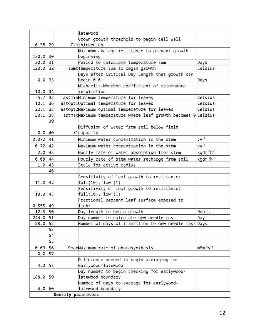
40          

1.0 1  Maximum value of parameter being used for each iteration0.01 2  Minimum value of parameter being used for each iteration0.1 3  Step size (DELTA) to begin iteration (in units of parameter)

0.001 4  Step size (TAU) to terminate iteration (in units of parameter)0.0001 5  Difference in Average Variance to Terminate Iteration

23

Table 6. Description of output parameters from ***.P output files

P(#) Name Description1 Day Day in year2 Tem Daily average temperature (˚C)3 Pre Daily precipitation (mm)4 Sm Soil moisture (kg m-3)5 PotTr Potential transpiration (kg H2O m-2 s-1)6 Trans Transpiration (kg H2O m-2 s-1)7 Rest Resistance of leaves to diffusion of CO2 (s m-1)8 Reswb Resistance of roots to water absorption (s m-1)9 Wab Water absorption by roots per unit volume of soil (kg m-3 day-1)10 Ci CO2 concentration inside the leaf (mM m-3)11 Phot Photosynthesis rate (mM CO2 m-2 s-1)12 Resp Respiration (maintenance) rate (mM CO2 day-1)13 Gleaf Growth rate of leaves (microns day-1)14 GRcamb Growth rate of cambial cells (microns day-1)15 GRenla Growth rate of enlarging cells (microns day-1)16 GRmat Growth rate of maturing cells (microns day-1)17 Groot Growth rate of roots (microns day-1)18 SuL Sucrose in leaves (mM CO2)19 SuS Sucrose in the stem (mM CO2)20 SuR Sucrose in roots (mM CO2)21 d13Cps Carbon isotope composition of photosynthate (‰)22 d13CstL Carbon isotope composition of stored starch in leaves (‰)23 d13CstS Carbon isotope composition of stored starch in the stem (‰)24 d13CstR Carbon isotope composition of stored starch in roots (‰)25 d13CL Carbon isotope composition of cellulose in leaves (‰)26 d13CS Carbon isotope composition of cellulose in the stem (‰)27 d13CR Carbon isotope composition of cellulose in roots (‰)28 dDps Hydrogen isotope composition of photosynthate (‰)29 dDstL Hydrogen isotope composition of stored starch in leaves (‰)30 dDstS Hydrogen isotope composition of stored starch in the stem (‰)31 dDstR Hydrogen isotope composition of stored starch in roots (‰)32 dDCL Hydrogen isotope composition of cellulose in leaves (‰)33 dDCS Hydrogen isotope composition of cellulose in the stem (‰)34 dDCR Hydrogen isotope composition of cellulose in roots (‰)35 d18Ops Oxygen isotope composition of photosynthate (‰)36 d18OstL Oxygen isotope composition of stored starch in leaves (‰)37 d18OstS Oxygen isotope composition of stored starch in the stem (‰)38 d18OstR Oxygen isotope composition of stored starch in roots (‰)39 d18OCL Oxygen isotope composition of cellulose in leaves (‰)40 d18OCS Oxygen isotope composition of cellulose in the stem (‰)41 d18OCR Oxygen isotope composition of cellulose in stem (‰)42 Ct Control on growth43 Ctm Control on cell maturation44 xleaf Mass of growing leaf tissue (kg)45 nr Total number of cells in growth ring46 nc Number of cells in the cambial stage47 ne Number of cells in the enlargement stage

24

48 nm Number of cells in the maturation stage49 dendgr Dendrograph trace50 dgrmin Dengrograph minimum51 dgmax Dendrograph maximum52 So-Si Source minus Sink (Photosynthesis minus Respiration + Growth in leaf, stem, root)53 stemw Concentration of water in the stem54 C balan Carbon balance at end of day55 LimEnvLf Limiting environmental factor for leaf growth56 LimEnvRt Limiting environmental factor for root growth57 LimEnvDiv Limiting environmental factor for cell division58 LimEnvEnl Limiting environmental factor for cell enlargement59 LimEnvMat Limiting environmental factor for cell maturation60 d13CCel Carbon isotope composition of whole cell cellulose (‰)61 dDvap Hydrogen isotope composition of atmospheric vapor (‰)62 dDPrec Hydrogen isotope composition of precipitation (‰)63 dDXw Hydrogen isotope composition of xylem water (‰)64 dDLw Hydrogen isotope composition of leaf water (‰)65 dDCel Hydrogen isotope composition of cellulose formed during the day (‰)66 d18Ovap Oxygen isotope composition of atmospheric vapor (‰)67 d18OPrec Oxygen isotope composition of precipitation (‰)68 d18OXw Oxygen isotope composition of xylem water (‰)69 d18OLw Oxygen isotope composition of leaf water (‰)70 d18OCel Oxygen isotope composition of cellulose formed during the day (‰)71 waterloss Water loss from leaves per day72 MaxWLoss Maximum possible water loss from leaves per day73 DayLength Day length (seconds)74 MxCellSz Maximum cell size of new years growth cells75 Contr Control on growth rate of leaves 76 Contr2 Control to restart growth of leaves77 d13CstLAr Carbon isotope composition of stored starch in leaves (‰)78 d13CstSAr Carbon isotope composition of stored starch in stem (‰)79 d13CstRAr Carbon isotope composition of stored starch in roots (‰)

25

III. REFERENCES

Carey, E.V., DeLucia, E.H., Ball, J.T. 1986. Stem maintenance and construction respiration in Pinus ponderosa grown in different concentrations of atmospheric CO2 .Tree Phys. 16:125-130.

Craig H. and Gordon L.I. 1965. Deuterium and oxygen-18 variations in the ocean and the marine atmosphere. In E. Tongiorgi. Proceedings of a conference on Stable Isotopes in Oceanographic Studies and Paleotemperatures 9-130. Spolito, Italy.

Denne M. P. and Dodd R.S. 1981. The environmental control of xylem differentiation. In: Barnett, J. R. (ed.) Xylem Cell Development. Castle House Publ., London, 236-255.

Farquhar G.D., O’Leary M.H. and Berry J.A. 1982. On the relationship between carbon isotope discrimination and the intercellular carbon dioxide concentration in leaves. Australian Journal of Plant Physiology 9:121-137.

Flanagan L.B. & Ehleringer J.R. 1991. Effects of mild water stress and diurnal changes in temperature and humidity on the stable oxygen and hydrogen isotopic composition of leaf water in Cornus stolonifera L. Plant Physiology 97:298-305.

Fondy B.R. and Geiger D.R. 1982. Diurnal pattern of translocation and carbohydrate metabolism in source leaves of Beta vulgaris. Plant Physiology 70:671-676.

Freidli, H., Lötscher, H., Oeschger, H., Seigenthaler, U., and Stauffer, B. 1986. Ice core record of the 13C/12C ratio of atmospheric CO2 in the past two centuries. Nature 324, pp. 237-238.

Fritts H.C., Shashkin A.S. and Downes G.M. 1999. TreeRing 3: A simulation model of conifer ring growth and cell structure. In Wimmer, R. and R. E. Vetter. Tree Ring Analysis: Biological, Methodological and Environmental Aspects. CAB International, Wallingford. UK. pp. 3-32.

Hansen P. 1967. 14C-studies on apple trees III. The influence of season on storage and mobilization of labeled compounds. Physiologia Plantarum 20:1103-1111.

Hemming D.L., Switsur V.R., Waterhouse J.S. Heaton T.H.E. and Carter A.H.C. 1998. Climate variation and the stable carbon isotope composition of tree ring cellulose: an intercomparison of Quercus robur, Fagus sylvatica and Pinus silvestris. Tellus 50B: 25-33.

Hemming D.L., Jalkanen R. and Leavitt S.W. 2001. Preliminary relationships between climate and the apical extension, needle production and ring width of Pinus ponderosa in Arizona, USA. Palaeobotanist 50:125-131.

Keeling, C. D. and Whorf-T. P. 1996. Atmospheric CO2 records from sites in the SIO air sampling network. In: Trends: A compendium of data on global change. Carbon Dioxide Information Analysis Centre, Oak Ridge National Laboratory, Oak Ridge, Tenn., U.S.A.

26

Lacointe A., Kajji A., Daudet F-A., Archer P. and Frossard J-S. 1993. Mobilization of carbon reserves in young walnut trees. Acta Botanica Gallica 140(4): 435-441.

Landsberg, J.J. 1986. Physiological ecology of forest production. Academic Press, London p89.

Levin, I., Kromer, B., Schoch-Fischer, H., Bruns, M., Münnich, M., Berdau, D., Vogel, J. C., Münnich, K. O. 1996. 13C records from sites in Central Europe. In: Trends ’93: A compendium of data on global change. (eds Boden, T. A., Kaiser, D. P., Sepanski, R. J. and Stoss, F. W.). ORNL/CDIAC-65. Carbon Dioxide Information Analysis Centre, Oak Ridge National Laboratory, Oak Ridge, Tenn., U.S.A.

Majoube M. 1971. Fractionnement en oxygène-18 et en deuterium entre l’eau et sa vapeur. Journal of Chemical Physics 197:1423-1436.

Merlivat L. 1978. Molecular diffusivities of H216O, HD16O and H2

18O in gases. Journal of Chemistry and Physics 69:2864-2871.

Monserud R.A. and Marshall J.D. 1999. Allometric crown relations in three northern Idaho conifer species. Canadian Journal of Forest Research 29:521-535. Table 5.

O’Leary, M.H. 1981. Carbon isotope fractionation in plants. Phytochemistry 20:553-567.

Roden J.S., Lin G. and Ehleringer J.R. 2000. A mechanistic model for interpretation of hydrogen and oxygen isotope ratios in tree-ring cellulose. Geochimica et Cosmochimica Acta 64(1), 21-35.

Ryan, M. G., Gower, S. T., Hubbard, R. M., Waring, R. H., Gholz, H. L., Cropper, W. P. Jr., Running, S. W. 1995. Woody tissue maintenance respiration of four conifers in contrasting climates. Oecologia 101:133-140.

Silkin, P.P. 2001. Cell wall masses of conifer tree rings. In: Tree-rings and People. Abstract International Conference on the Future of Dendrochronology, Davos 22-26 Sept 2001. WSL, CH-8903 Birmensdorf 2001, p.202-203.

Taiz L. and Zeiger E. 1991. Plant Physiology. Benjamin/Cummings Publishing Co., CA.

Wardlaw I.F. 1990. The control of carbon partitioning in plants. New Phytologist 116:341-381.

Yakir D. and DeNiro M.J. 1990. Oxygen and hydrogen isotope fractionation during cellulose metabolism in Lemna gibba L. Plant Physiology 93:325-332.

27