Hahn, Hubert

Model Based Control of a Parallel Robot – A Comparison of Control Algo-rithms

In this contribution the control behavior of a special construction of a parallel robot, called multi-axes test facility, isinvestigated. After a brief discussion of the different tasks of the robot the construction of the robot is briefly presented.To solve the tasks, different control algorithms are derived based on model equations of different complexity of therobot. Depending on the task to be performed by the robot, the controllers compensate the kinematic and/or kineticcoupling of the degrees of freedom of the robot, stabilize the system and achieve the desired spatial motion of eachdegree of freedom as well as sufficient robustness with respect to parameter uncertainties and load variations. A fewresults obtained in computer simulations and laboratory experiments are presented and judged with respect to thequality of control, the closeness to reality of the computer simulations, and the amount of costs and work needed torealize the different solutions.

1. Tasks and construction of the parallel robot

The task of these investigations was to develop and construct a parallel robot for the following purposes: manipulatorfor precise, rapid, and large spatial motions, test facility for spatial vibration and transient tests of components andsystems, flight and motion simulator, instrument for experimental testing of different (e.g. redundant and nonredundant) actuator configurations and sensor and observer configurations, and as a vehicle for implementation andexperimental testing of different controller and identification algorithms and safety concepts.

In this project the following types of parallel robots have been investigated theoretically, numerically, and in labora-tory experiments: hexapodes (HEX) (Stewart platforms) and spatial multi-axes test facilities (MAP) with differentactuator and sensor configurations (Figures 1(a) and 1(b)). The special parallel robot discussed here is a multi-axestest facility driven by six to eight servo-pneumatic actuators (Figure 1(c)). Compared to hexapodes this specialconstruction has the advantage that its symmetry is not completely lost by including redundant actuator configura-tions. Servo-pneumatic actuators (instead of electrical or servo-hydraulic actuators) have been chosen because theseactuators are low cost components, the medium gas is everywhere available (advantages), and because gas has ahigh compressibility, a low viscosity, and is governed by complex nonlinear model equations of the pressure evolutionin the actuator chambers (challenge for the control design). As a consequence, the combination of a parallel robotwith servo-pneumatic actuators is a new interesting mechatronic system which requires sophisticated model-basedcontrol algorithms.

test table

actuatorpayload

frame

base

(a) multi-axes test facility (MAP)

tool

end-effector

actuator

frame

base

(b) hexapode (HEX) (c) photograph of a MAP developed at RTS

Figure 1: Alternative constructions of parallel robots

PAMM · Proc. Appl. Math. Mech. 2, 124–127 (2003) / DOI 10.1002/pamm.200310048

Important design aspects of the robot are ([1]): a stiff frame (30 Hz < eigenfrequencies), which is flexible enoughto enable the attachment of between six and eight actuators, a rigid but light test table made of aluminum, twodifferent types of (stiff and adjustable) universal joints (to avoid clearances), servo-pneumatic drives that provide adesired trade-off between leakage flow and friction, more than 50 position, velocity, acceleration, pressure and forcesensors, integrated within the actuators, a powerful electronic hardware to enable flexible implementation, testing,and real time operation of the various control and identification algorithms, and a sophisticated safety system.The following sensing elements are integrated in the actuators: magnetostrictive displacement and velocity sensors,capacitive acceleration sensors, piezoresistive pressure sensors, and DMS force sensors. The measured signals areused for linear and nonlinear control, for experimental identification of the model parameters, in the safety system,and for signal processing. A dSPACE multiprocessor system with 2 DEC Alpha processors, 4 signal processors, 128A/D input channels, and 32 D/A output channels is used as the controller hardware.

2. Mathematical models of the robot

The robot has been built for different purposes and tasks. As a model of a system depends on its purpose, severalmodels of the robot were required which serve as a basis for the design of the different controllers. The followingmodel has been used as a basis for all theoretical and numerical investigations. It has the bilinear state-space form

x = a(x) + b(x) · u , y = x1 (1)

with the state vector x =(xT

1 , xT2 , xT

3 , xT4 , xT

5

) ∈ IR36, and with u ∈ IR6 as the input vector of the servo-valvesx1 ∈ IR6 as the vector of the degrees of freedom (DOF) of the test table or end-effector, x2 ∈ IR6 as the velocitiesassociated with x1, x3 ∈ IR6 and x4 ∈ IR6 as the pressures in the 12 chambers of the six pneumatic actuators, andx5 ∈ IR12 as the vector of the positions and velocities of the six servo-valve pistons. The vector fields a(x) and b(x)are partitioned, in agreement with the state vector, as

a(x) =(aT

m(x1, x2), aTpI(x), aT

pII(x), aTV (x5)

)T and b(x) =(bT

m(x1, x2), bTpI(x3, x4), bT

pII(x3, x4), bTV

)T

The nonlinear subsystem(am(x1, x2), bm(x1, x2)

)defines a nonlinear differential equation (DE) of 12th order that

describes the spatial motion of the test table. It includes both the kinematic and the kinetic behavior of the 13-rigid-body mechanism. These DEs are obtained by symbolic elimination of 144 dependent coordinates and 72 Lagrangemultipliers from the underlying differential algebraic equations of the robot that are set up by 78 kinematic DEs,78 kinetic DEs of the 13 rigid bodies (test table, six actuator pistons, and six actuator housings), and 72 algebraicconstraint equations that describe the six spherical , six universal, and six prismatic joints of the six actuators(see [2, 3]). The subsystem

(apI(x), apII(x), bpI(x), bpII(x)

)defines a nonlinear DE of 12th order that describes

the pressure evolution in the 12 actuator chambers and the mass flows over the control edges of the servo-valves.(see [4]). The remainder subsystem

(aV (x5) = AV · x5 and bV = BV

)defines a linear DE of 12th order that

describes the motion of the six pistons of the servo-valves. This model will be called subsequently NMNPLV-model, where NM stands for nonlinear model of the 13-body mechanism, NP for the nonlinear pneumatic modelof the actuators, and LV for the linear valve mechanics. Depending on the task to be performed by the robot, thefollowing simplified submodels and their combinations have been used in the design of the different controllers: RMas reduced nonlinear model of the robot mechanics based on a single rigid body with modified inertia parametersthat were adapted to the 13-mass model, LM as linear reduced model of the robot mechanics, LP as linear modelof the actuator pneumatics, and TV as trivial model (static linear model) of the valve mechanics. If a controlalgorithm is based on the trivial valve model TV, this abbreviation will be omitted in the name of the controller.Different combinations of the above submodels are used in computer simulations, model parameter identification,controller design, and the design of the safety system. The plant model (NMNPLV) includes the nonlinear robotkinematics and the nonlinear robot kinetics of the 13-rigid-body mechanism (NM), the nonlinear actuator friction,nonlinear actuator pneumatics (NP), the linear valve dynamics (LV), and bounded control input signals.

3. Controller design

In the computer simulations and laboratory experiments the following controllers are used that have been derived onthe basis of different subsystem models of the robot: conventional linear PD and MS (multi-sensor) controllerswith nonlinear kinematic decoupling prefilters obtained by standard trial and error approaches; computed torquecontrollers CT-LM-P, CT-RM-P, CT-NM-P obtained on the basis of the models LM, RM, and NM, where Pstands for additional controllers of the actuator pressures; I/O-linearization controllers EL-RMLP and EL-RMNP; a gain-scheduling controller GS obtained on the basis of the symbolic linear model equations LMLPTVand using x1 as the scheduling vector; and a sliding-mode controller SM including an EL-RMNP controller and

Section 3: Multibody Systems and Kinematics 125

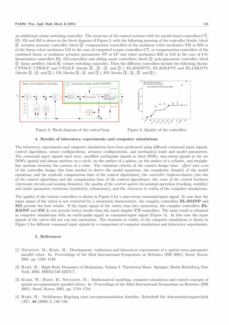
an additional robust switching controller. The structure of the control systems with the model-based controllers CT,EL, GS and SM is shown in the block diagram of Figure 2, with the following meaning of the controller blocks: block�2 actuator pressure controller; block �3 compensation controllers of the nonlinear robot mechanics NM or RM or

of the linear robot mechanics LM in the case of computed torque controllers CT, or compensation controllers of thecombined linear or nonlinear actuator pneumatics NP or LP and robot mechanics RM or LM in the case of I/0-linearization controllers EL, GS-controllers and sliding mode controllers; block �4 pole-placement controller; block�5 linear prefilter; block �6 robust switching controller. Then the different controllers include the following blocks:

CTNM-P, CTRM-P, and CTLM-P (blocks �2 , �3 , �4 and �5 ); EL-RMNPTV, EL-RMLPTV and EL-LMLPTV(blocks �3 , �4 and �5 ); GS (blocks �3 , �4 and �5 ); SM (blocks �3 , �4 , �5 and �6 ).

5

4

3

62

linear and nonlinear controllers

xd

xd

xdx2

x2

x1, x2

x3, x4 x1, x2

−++

1

kinetics andkinematics

actuatorsx1

real plant or plant model NMNPLV

xd servo-valves

robot++ + x3, x4

−

++

...x d

Figure 2: Block diagram of the control loop

0

0.01

0.02

0.03

0.04

0.05

tota

l per

form

ance

inde

x J t

P, PD MS

CT−LM−P

CT−RM−P

CT−NM−P

EL−LMLP

EL−RMLP GS

EL−RMNP SM

sine sweep command input signal

bounded controller outputunbounded controller output

Figure 3: Quality of the controllers

4. Results of laboratory experiments and computer simulations

The laboratory experiments and computer simulations have been performed using different command input signals,control algorithms, sensor configurations, actuator configurations, and mechanical loads and model parameters.The command input signals used were: modified earthquake signals in three DOFs, sine-sweep signals in the sixDOFs, spatial and planar motions on a circle, on the surface of a sphere, on the surface of a cylinder, and straight-line motions between the corners of a cube. The valuation criteria of the control design were: effort and costsof the controller design (the time needed to derive the model equations, the complexity (length) of the modelequations, and the symbolic computation time of the control algorithms), the controller implementation (the sizeof the control algorithms and the computation time of the control algorithms), the costs of the control hardware(electronic circuits and sensing elements), the quality of the control system (in nominal operation (tracking, stability)and under parameter variations (sensitivity, robustness)), and the closeness to reality of the computer simulations.

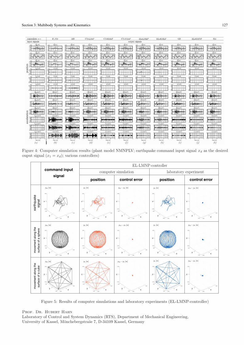
The quality of the various controllers is shown in Figure 3 for a sine-sweep command-input signal. In case that theinput signal of the valves is not restricted by a saturation characteristic, the complex controllers EL-RMNP andSM provide the best results. If the input signal of the valves runs into saturation, the complex controllers EL-RMNP and SM do not provide better results than the much simpler CT-controllers. The same result is obtainedin computer simulations with an earth-quake signal as command-input signal (Figure 4). In this case the inputsignals of the valves did not run into saturation. The closeness to reality of the computer simulations is shown inFigure 5 for different command input signals by a comparison of computer simulations and laboratory experiments.

5. References

[1] Neumann, M.; Hahn, H.: Development, realization and laboratory experiments of a spatial servo-pneumaticparallel robot. In: Proceedings of the 32nd International Symposium on Robotics (ISR 2001). Seoul, Korea,2001, pp. 1533–1538.

[2] Hahn, H.: Rigid Body Dynamics of Mechanims, Volume I: Theoretical Basis. Springer, Berlin Heidelberg NewYork, 2002. ISBN3-540-42373-7.

[3] Klier, W.; Hahn, H.; Neumann, M.: Mathematical modeling, computer simulation and control concepts ofspatial servopneumatic parallel robots. In: Proceedings of the 32nd International Symposium on Robotics (ISR2001). Seoul, Korea, 2001, pp. 1719–1724.

[4] Hahn, H.: Nichtlineare Regelung eines servopneumatischen Antriebs. Zeitschrift fur Automatisierungstechnik(AT), 48 (2000) 3, 140–150.

PAMM · Proc. Appl. Math. Mech. 2 (2003) 126

(b) (c) (d) (e) (f) (g) (h) (i) (j) (k)

Figure 4: Computer simulation results (plant model NMNPLV; earthquake command input signal xd as the desiredouput signal (x1 = xd); various controllers)

eart

hqua

kesu

rfac

e of

a c

ube

mov

emen

t alo

ng th

em

ovem

ent a

long

the

control error control error

command input

signalposition

sign

alsu

rfac

e of

a s

pher

e

position

−0.05

0

0.05

−0.05

0

0.05

−0.05

0

0.05

−0.05

0

0.05

−0.05

0

0.05

−0.05

0

0.05

−0.05

0

0.05

−0.05

0

0.05

−0.05

0

0.05

−0.05

0

0.05

−0.05

0

0.05

−0.05

0

0.05

−0.05

0

0.05

−0.05

0

0.05

−0.05

0

0.05

−0.05

0

0.05

−0.05

0

0.05

−0.05

0

0.05

−0.05

0

0.05

−0.05

0

0.05

−0.05

0

0.05

−0.05

0

0.05

−0.05

0

0.05

−0.05

0

0.05

−0.05

0

0.05

−0.05

0

0.05

−0.05

0

0.05

−0.05

0

0.05

−0.05

0

0.05

−0.05

0

0.05

−0.05

0

0.05

−0.05

0

0.05

−0.05

0

0.05

−0.05

0

0.05

−0.05

0

0.05

−0.05

0

0.05

−0.05

0

0.05

−0.05

0

0.05

−0.05

0

0.05

−0.05

0

0.05

−0.05

0

0.05

−0.05

0

0.05

−0.05

0

0.05

−0.05

0

0.05

−0.05

0

0.05

y

z

x

y

z

x

y

z

x

y

z

x

y

z

x

y

z

x

y

z

xy

z

x

y

z

x

y

z

x

y

z

x

y

z

x

y

z

xy

z

x

y

z

x

EL-LMNP-controller

laboratory experimentcomputer simulation

p0d − p0 [m]p0 [m] p0d − p0 [m]p0 [m]

p0d − p0 [m]p0 [m]

p0d − p0 [m]p0 [m]

p0d [m]

p0d [m]

p0d [m] p0 [m]

p0 [m] p0d − p0 [m]

p0d − p0 [m]

Figure 5: Results of computer simulations and laboratory experiments (EL-LMNP-controller)

Prof. Dr. Hubert HahnLaboratory of Control and System Dynamics (RTS), Department of Mechanical Engineering,University of Kassel, Monchebergstrase 7, D-34109 Kassel, Germany

(a)

Section 3: Multibody Systems and Kinematics 127