Embed Size (px)
Citation preview

1
Model-based appraisal of minimum unit pricing for
alcohol in the Republic of Ireland
An adaptation of the Sheffield Alcohol Policy Model version 3
September 2014
Colin Angus
Yang Meng
Abdallah Ally
John Holmes
Alan Brennan
©ScHARR, University of Sheffield

2
1 CONTENTS 1 Contents .......................................................................................................................................... 2
1.1.1 Index of Tables ................................................................................................................ 5
1.1.2 Index of Figures ............................................................................................................... 7
2 Executive summary ......................................................................................................................... 8
2.1 Main conclusions .................................................................................................................... 8
2.2 Research questions ................................................................................................................. 8
2.3 Methods used ......................................................................................................................... 8
2.4 Summary of model findings .................................................................................................... 9
2.4.1 Patterns of drinking and expenditure ............................................................................. 9
2.4.2 Effect of modelled policies on consumption and expenditure ..................................... 10
2.4.3 Effects of modelled policies on alcohol-related harms ................................................. 11
3 Introduction .................................................................................................................................. 13
3.1 Background ........................................................................................................................... 13
3.2 Research questions addressed ............................................................................................. 13
4 Methods ........................................................................................................................................ 14
4.1 Overview of SAPM3 .............................................................................................................. 14
4.2 Modelling the link between intervention and consumption ................................................ 15
4.2.1 Overview ....................................................................................................................... 15
4.2.2 Consumption data ......................................................................................................... 15
4.2.3 Patterns of consumption .............................................................................................. 19
4.2.4 Prices ............................................................................................................................. 20
4.2.5 Beverage preferences ................................................................................................... 25
4.2.6 Price elasticities of alcohol demand ............................................................................. 27
4.2.7 Modelling the impact of interventions on price ........................................................... 30
4.2.8 Modelling the impact of price on consumption ........................................................... 32
4.3 Modelling the relationship between consumption and harm .............................................. 33
4.3.1 Model structure ............................................................................................................ 33
4.3.2 Alcohol-related health conditions ................................................................................. 33
4.3.3 Alcohol-attributable fractions and potential impact fractions ..................................... 35
4.3.4 Applying potential impact fractions .............................................................................. 36
4.4 Consumption to health harms model ................................................................................... 37
4.4.1 Mortality model structure ............................................................................................ 37
4.4.2 Morbidity model structure............................................................................................ 39

3
4.4.3 Time lag effects for chronic harms ............................................................................... 40
4.4.4 Mortality model parameters ......................................................................................... 40
4.4.5 Morbidity model parameters ........................................................................................ 40
4.5 Consumption to crime harms model .................................................................................... 43
4.5.1 Summary of crime model structure .............................................................................. 43
4.5.2 Baseline volumes of crime ............................................................................................ 44
4.5.3 Crime risk function parameters .................................................................................... 45
4.6 Consumption to workplace harms model ............................................................................. 46
4.6.1 Summary of workplace model structure ...................................................................... 46
4.6.2 Baseline absence data ................................................................................................... 46
4.6.3 Workplace risk function parameters ............................................................................ 48
4.7 Sensitivity analyses ............................................................................................................... 48
5 Results ........................................................................................................................................... 50
5.1 Summary results for all policies ............................................................................................ 50
5.1.1 Impact on alcohol consumption ................................................................................... 50
5.1.2 Impact on consumer spending ...................................................................................... 54
5.1.3 Impact on retailers and the Exchequer ......................................................................... 59
5.1.4 Impact on health outcomes .......................................................................................... 61
5.1.5 Impact on crime outcomes ........................................................................................... 70
5.1.6 Impact on workplace outcomes .................................................................................... 73
5.1.7 Impact on societal costs ................................................................................................ 75
5.2 Example policy analysis A: 90c MUP ..................................................................................... 77
5.3 Example policy analysis B: 100c MUP ................................................................................... 85
5.4 Sensitivity analyses ............................................................................................................... 92
6 Discussion ...................................................................................................................................... 95
6.1 Differential policy impacts .................................................................................................... 95
6.2 Impacts by drinker group ...................................................................................................... 96
6.3 Impacts by income ................................................................................................................ 96
6.4 Impacts on revenue to the exchequer and retailers............................................................. 97
6.5 Impacts on alcohol-related health ........................................................................................ 98
6.6 Impacts on alcohol-related crime ......................................................................................... 99
6.7 Impacts on work absence ..................................................................................................... 99
6.8 Cost impacts on society ........................................................................................................ 99
6.9 Potential impact of MUP and price-based promotions ban on cross-border shopping ....... 99

4
6.10 Relative merits of MUP and price-based promotions ban in comparison with tax increases.
100
7 References .................................................................................................................................. 101
8 Appendix A .................................................................................................................................. 104

5
1.1.1 Index of Tables
Table 4.1: Proportion of alcohol sold in Ireland below a range of MUP thresholds............................. 23
Table 4.2: Elasticity estimates from the Irish and English Tobit models and the final adjusted Irish
figures ................................................................................................................................................... 28
Table 4.3: Pseudo-panel elasticity estimates for the UK ...................................................................... 29
Table 4.4: Method and assumptions to estimate threshold prices under BBCS: estimated duty plus
VAT per standard drink for beer, cider, wine, spirits and RTDs in Ireland ............................................ 31
Table 4.5: Health conditions included in the model ............................................................................. 34
Table 4.6: Morbidity model parameters estimated from HIPE data .................................................... 42
Table 4.7: Multipliers relating recorded crime volumes to estimated actual volumes ........................ 44
Table 4.8: Baseline crime volumes ........................................................................................................ 45
Table 4.9: AAFs for absenteeism calculated from NADS data .............................................................. 48
Table 5.1: Summary of estimated effects of pricing policies on alcohol consumption – absolute and %
change in consumption per drinker ...................................................................................................... 51
Table 5.2: Summary of estimated effects on alcohol consumption by income and drinker group ..... 52
Table 5.3: Summary of estimated effects of pricing policies on consumer spending – absolute and %
change in consumption per drinker per year ....................................................................................... 56
Table 5.4: Summary of estimated effects on consumer spending by income and drinker group ........ 57
Table 5.5: Summary of estimated effects of pricing policies on retailer and duty/VAT revenue-
absolute and % change ......................................................................................................................... 60
Table 5.6: Summary of policy impacts on health outcomes – changes in alcohol-related deaths,
hospital admissions and QALYs per year at full effect (20 years) ......................................................... 62
Table 5.7: Income specific health outcomes – policy impacts on deaths and hospital admissions per
year per 100,000 population at full effect (20 years) ........................................................................... 63
Table 5.8: Summary of policy impacts on alcoholic liver disease outcomes at full effect (20 years) ... 66
Table 5.9: Summary of impact of policies on annual deaths by condition type ................................... 67
Table 5.10: Summary of impact of policies on annual hospital admissions by condition type ............ 68
Table 5.11: Impact of modelled policies on annual crime volumes ..................................................... 71
Table 5.12: Estimated changes in annual crime volumes by crime category ....................................... 72
Table 5.13: Estimated changes in workplace absence.......................................................................... 74
Table 5.14: Summary of financial valuation of impact of modelled policies on health, crime and
workplace related harm in year 1 and cumulatively over 20 years ...................................................... 76
Table 5.15: Detailed consumption and spending results for 90c MUP ................................................ 79
Table 5.16: Detailed income and drinker group-specific results for 90c MUP ..................................... 80
Table 5.17: Relative changes in price, consumption and spending, by beverage type and location for
90c MUP ................................................................................................................................................ 81
Table 5.18: Detailed full effect health outcomes by drinker group and income for 90c MUP ............. 82
Table 5.19: Detailed breakdown of deaths and hospital admissions averted by health condition type
for 90c MUP .......................................................................................................................................... 83
Table 5.20: Effects of 90c MUP on death and hospital admissions by drinker group .......................... 83
Table 5.21: Effects of 90c MUP on deaths and hospital admissions by income group ........................ 83
Table 5.22: Detailed consumption and spending results for 100c MUP .............................................. 87
Table 5.23: Detailed income and drinker group-specific results for 100c MUP ................................... 88
Table 5.24: Relative changes in price, consumption and spending, by beverage type and location for
100c MUP .............................................................................................................................................. 89

6
Table 5.25: Detailed full effect health outcomes by drinker group and income for 100c MUP ........... 89
Table 5.26: Detailed breakdown of deaths and hospital admissions averted by health condition type
for 100c MUP ........................................................................................................................................ 90
Table 5.27: Effects of 100c MUP on death and hospital admissions by drinker group ........................ 90
Table 5.28: Effects of 100c MUP on deaths and hospital admissions by income group ...................... 90
Table 5.29: Comparison of estimated impacts on alcohol consumption for a 90c MUP and off-trade
promotion ban using alternative elasticity estimates .......................................................................... 92
Table 8.1: Modelled time-lags by condition – proportion of overall change in risk experienced in each
year following a change in consumption taken from Holmes et al 2012 ........................................... 104

7
1.1.2 Index of Figures
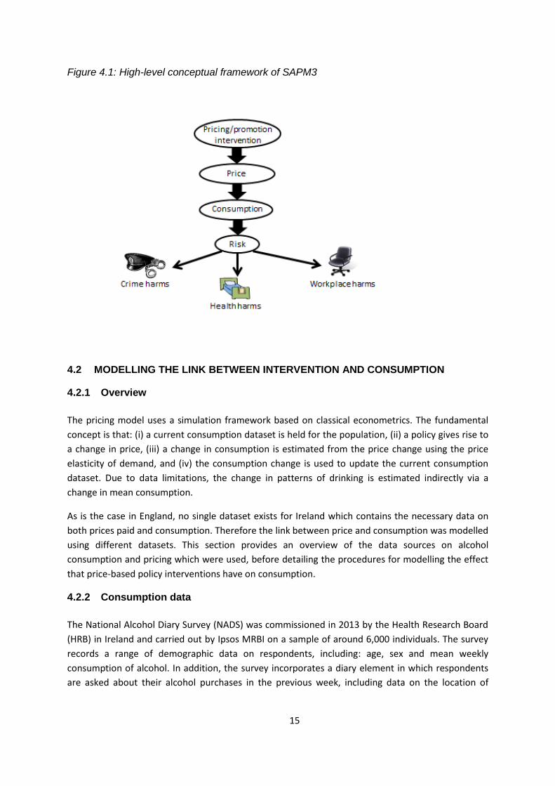
Figure 4.1: High-level conceptual framework of SAPM3 ...................................................................... 15
Figure 4.2: Distribution of mean weekly consumption (in standard drinks) by age group (NADS 2013)
.............................................................................................................................................................. 16
Figure 4.3: Distribution of mean weekly consumption by gender (NADS 2013) .................................. 17
Figure 4.4: Population distribution by drinker and income group (NADS 2013) .................................. 18
Figure 4.5: Distribution of peak day maximum consumption by gender (NADS 2013) ........................ 20
Figure 4.6: NADS (raw) and Neilsen (adjusted) price distributions for off-trade beverages (RTDs not
shown)................................................................................................................................................... 21
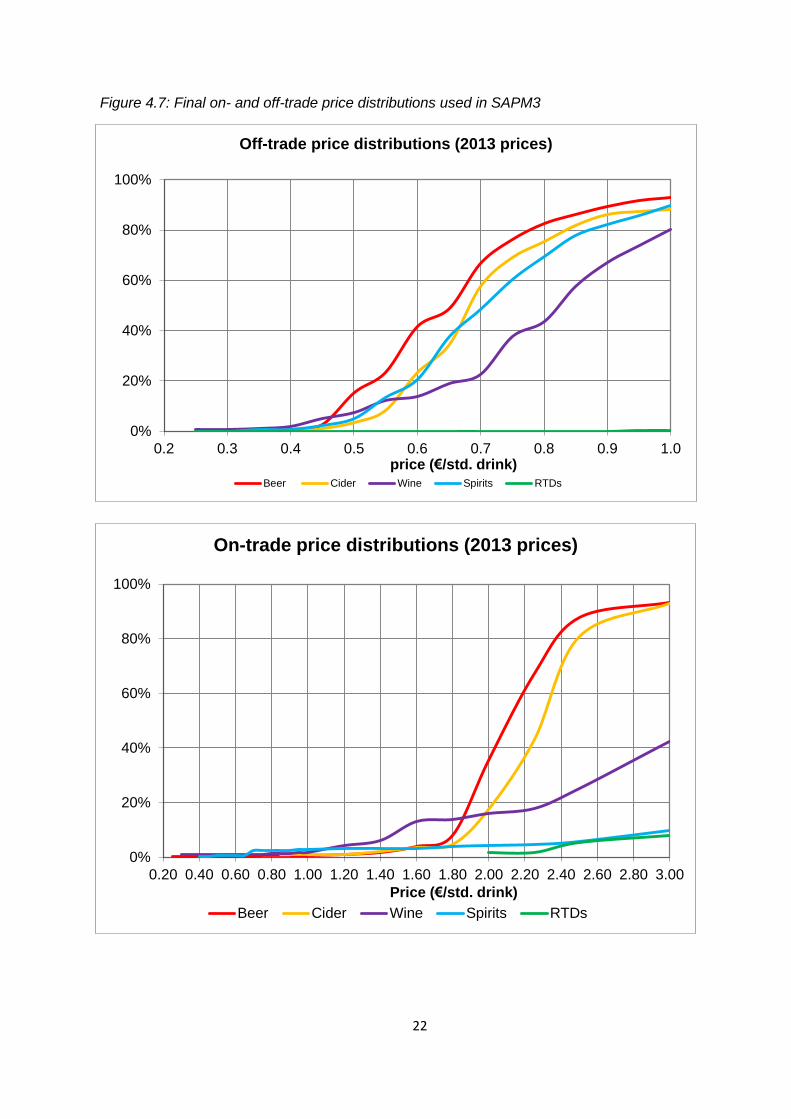
Figure 4.7: Final on- and off-trade price distributions used in SAPM3 ................................................. 22
Figure 4.8: Number and proportion of std. drinks purchased at below 90c by income and drinker
group ..................................................................................................................................................... 24
Figure 4.9: Proportion of total consumption and spending by drinker group...................................... 25
Figure 4.10: Consumption preferences by gender ............................................................................... 26
Figure 4.11: Consumption preferences by age ..................................................................................... 26
Figure 4.12: Consumption preferences by drinker group ..................................................................... 27
Figure 4.13: Consumption preferences by income group .................................................................... 27
Figure 4.14: Simplified mortality model structure ................................................................................ 38
Figure 4.15: Simplified structure of the morbidity model .................................................................... 39
Figure 4.16: Simplified structure of the crime model ........................................................................... 43
Figure 4.17: Illustrative linear relative risk function for a partially attributable acute harm (threshold
of 2.43 standard drinks) ........................................................................................................................ 46
Figure 4.18: Simplified structure of the workplace model ................................................................... 48
Figure 5.1: Summary of relative consumption changes by policy by drinker type ............................... 53
Figure 5.2: Summary of absolute consumption changes by policy by drinker type ............................. 53
Figure 5.3: Summary of relative consumption changes for MUP policies by drinker type .................. 54
Figure 5.4: Income-specific effects of different levels of MUP policy on consumption ....................... 54
Figure 5.5: Summary of relative spending changes by policy by drinker type ..................................... 58
Figure 5.6: Summary of absolute spending changes by policy by drinker type.................................... 58
Figure 5.7: Income-specific effects of different levels of MUP on spending ........................................ 59
Figure 5.8: Summary of relative changes in deaths and hospital admissions per year at full effect ... 64
Figure 5.9: Income-specific reductions in deaths per year per 100,000 population ............................ 64
Figure 5.10: Income-specific reductions in hospital admissions per year per 100,000 population ..... 65
Figure 5.11: Estimated reductions in deaths over time for exemplar MUP policies ............................ 69
Figure 5.12: Estimated reductions in hospital admissions over time for exemplar MUP policies ....... 69
Figure 5.13: Summary of relative changes in alcohol-attributable crime volumes by drinker group .. 73
Figure 5.14: Summary of relative changes in workplace absence by drinker ...................................... 75
Figure 5.15: Effects of 90c MUP on deaths and hospital admissions by health condition ................... 84
Figure 5.16: Effects of 100c MUP on deaths and hospital admissions ................................................. 91
Figure 5.17: Comparison of estimated impacts on alcohol consumption of a 90c MUP policy using
alternative elasticity estimates ............................................................................................................. 93
Figure 5.18: Comparison of estimated impacts on alcohol consumption of an off-trade promotion
ban using alternative elasticity estimates............................................................................................. 93

8
2 EXECUTIVE SUMMARY
2.1 MAIN CONCLUSIONS
Estimates from the Irish adaptation of the Sheffield Alcohol Policy Model version 3 (SAPM3) suggest:
1. Minimum unit pricing policies (MUP) would be effective in reducing alcohol consumption,
alcohol-related harms (including alcohol-related deaths, hospitalisations, crimes and
workplace absences) and the costs associated with those harms.
2. A ban on below-cost selling (implemented as a ban on selling alcohol for below the cost of
duty plus the VAT payable on that duty) would have a negligible impact on alcohol
consumption or related harms.
3. A ban on price-based promotions in the off-trade, either alone or in tandem with an MUP
policy would be effective in reducing alcohol consumption, related harms and associated
costs.
4. MUP and promotion ban policies would only have a small impact on low risk drinkers.
Somewhat larger impacts would be experienced by increasing risk drinkers, with the most
substantial effects being experienced by high risk drinkers.
5. MUP and promotion ban policies would have larger impacts on those in poverty, particularly
high risk drinkers in poverty, than on those not in poverty. However; those in poverty also
experience larger relative gains in health and are estimated to very marginally save money
due to their reduced drinking under the majority of policies.
2.2 RESEARCH QUESTIONS
What is the estimated impact of MUP policies ranging from 40c to 120c per standard drink?
What is the estimated impact of a ban on below-cost selling?
What is the estimated impact of a ban on price-based promotions in the off-licensed trade?
How do these impacts vary by drinker group (low risk, increasing risk, high risk) and by
income group (in poverty, not in poverty)?
2.3 METHODS USED
The Sheffield Alcohol Policy Model (SAPM) has been used previously in England and in Scotland to
analyse the potential effects of pricing policies. We have developed a new version of the model to
incorporate data and evidence relating to the Republic of Ireland population.
The research has obtained data and evidence from available sources as follows:
Alcohol consumption – National Alcohol Diary Survey (NADS)
Alcohol prices in supermarkets and other off-trade outlets – Nielsen Ltd
Alcohol prices in pubs, bars and other on-trade outlets – NADS

9
Alcohol preferences and prices paid for different types of beverages by different population
subgroups – NADS
Price elasticities – previously published research
Hospital Discharge rates for Alcohol Related Diseases - Hospital In-Patient Enquiry (HIPE)
data
Mortality rates for Alcohol Related Diseases - National Drug-Related Death Index (NDRDI) &
General Mortality Register (GMR)
Costs of Healthcare for Alcohol Related Diseases – Healthcare Pricing Office (HPO) data
Crime Rates – Central Statistics Office publications of recorded crime rates & Garda
estimates of recording rates
Costs of Policing and Justice – Adjusted from UK Home Office estimates of unit costs of crime
using data from Hope et al. 2009
Work absence rates, work participation rates and average salary rates by population
subgroups – NADS & European Union – Statistics on Income and Living Conditions (EU-SILC)
The model synthesises all of this data and evidence and models the estimated impact of possible
future pricing policies on alcohol consumption patterns, spending, and health (both short-term and
over a long-term 20 year horizon).
2.4 SUMMARY OF MODEL FINDINGS
2.4.1 Patterns of drinking and expenditure
F1. The evidence estimates that within the overall population aged 18+, the proportion of people
who don’t drink, drink at low risk (less than 16.8 std. drinks per week for men and 11.2 for women),
increasing risk (16.8-40 std. drinks per week for men and 11.2-28 for women), and high risk (more
than 40 std. drinks per week for men and 28 for women) levels are 22.1%, 56.3%, 16.4% and 5.2%
respectively1.
F2. Low risk drinkers consume on average 4.5 standard drinks per week, spending €508 per annum
on alcohol. Increasing risk drinkers consume 21.9 standard drinks per week, spending €2,218 per
annum and high risk drinkers consume on average 62.5 standard drinks per week, spending €5,120
per annum. These patterns differ somewhat when examined by income group, with high risk
drinkers in poverty (1.0% of the population) estimated to drink 75.3 standard drinks per week,
spending €5,055 per annum, whilst high risk drinkers above the defined poverty line (4.2% of the
population) consume 59.5 standard drinks per week and spend €5,136 a year.
F3. Overall, increasing risk and high risk drinkers combined (22% of the population) account for 66%
of all alcohol consumption and 61% of all spending on alcohol.
F4. Prices vary by type of beverage. When examining a potential minimum price for a standard drink
(a floor price below which no alcohol may legally be sold) of 90c, the evidence suggests that 89.4%
1 These categorisations are based on average consumption levels only and do not account for patterns in
consumption, as there is no clear international consensus on how to combine both factors into a single categorisation; however these patterns are accounted for in all modelling work presented in this report
10
of off-trade beer, 66.9% of off-trade wine, and 79.9% of off-trade spirits sold in the year 2013 would
be affected and incur a price rise. Overall, an estimated 64%, 79% and 87% of the off-trade drinks
sold would be affected by an 80c, 90c and 100c minimum unit price (MUP) respectively.
2.4.2 Effect of modelled policies on consumption and expenditure
F5. For a 90c MUP, the estimated reduction in alcohol consumption per drinker2 for the overall
population is 6.2%. In absolute terms this equates to an annual reduction of 38.7 standard drinks per
drinker per year. The equivalent figures for a 100c MUP are 8.8% and 55.4 standard drinks. The
lower modelled MUP policies are estimated to have very small impacts; however, effectiveness
increases steeply at 70c and above (70c = -1.9%, 80c = -3.8%, 90c= -6.2%).
F6. High risk drinkers have much larger estimated consumption reductions for MUP policies than
increasing risk or low risk drinkers. For a 90c MUP the estimated reductions are 10.7% for high risk
drinkers, 5.1% for increasing risk drinkers and 1.9% for low risk drinkers. Differences in absolute
consumption reductions are significantly larger, with high risk drinkers reducing their consumption
by 350 standard drinks per year (6.7 per week) for a 90c MUP, compared to a reduction of 58 for
increasing risk drinkers and 4.4 standard drinks per year for low risk drinkers. Absolute reductions
are also larger for those in poverty (e.g. a reduction of 57.7 standard drinks per year vs. 34.8 on
average for those not in poverty). This demonstrates that MUP policies are well targeted, achieving a
higher proportional reduction in consumption amongst increasing and high risk drinkers than
amongst the majority of drinkers who drink at low risk levels.
F7. A ban on below-cost selling is estimated to have almost no impact on population consumption (-
0.0%), spending (+50c per drinker per year), health outcomes (166 fewer hospital admissions per
year) or crime (3 fewer crimes per year).
F8. A ban on off-trade promotions is estimated to have a similar impact to a 70c MUP, with an
estimated reduction in average consumption of 1.8%, leading to 45 fewer alcohol-related deaths and
1,382 fewer hospital admissions. As with MUP policies a promotion ban is well targeted, with higher
proportional consumption reductions amongst increasing and high risk drinkers.
F9. Under MUP and promotion ban policies, drinkers are estimated to reduce consumption but pay
slightly more on average per standard drink consumed, and so estimated percentage changes in
spending are smaller than estimated changes in consumption. For all modelled policies, spending
across the whole population is estimated to increase, for example by €14.90 (+1.27%) per drinker
per year for a 90c MUP alongside a consumption change of –6.2%. Spending changes also differ
across the population, with high risk drinkers estimated to have a small saving of €35.80 (-0.70%) per
year whilst low risk drinkers spending increases by €18.50 (+0.84%) per year under a 90c MUP.
Those in poverty are estimated to reduce spending under the majority of policies, whilst those not in
poverty increase their spending (e.g. -€15.70 and +€21.20 per year respectively under a 90c MUP).
F10. Under all modelled policies revenue to the Exchequer (from duty and VAT receipts) is estimated
to decrease slightly, with a 1.3% reduction (equivalent to €21.4m) for a 90c MUP. This is likely to be
2 Here, and elsewhere in this report, consumption reductions are reported per drinker unless explicitly stated
otherwise
11
at least partially offset by a reduction in VAT reclaims from retailers selling alcohol for below cost
price. Revenue to retailers is estimated to increase across all policies, with an increase of €62.6m
(3.8%) under a 90c MUP. The vast majority of this is accrued in the off-trade, although on-trade
retailers are estimated to gain slightly under MUP policies (e.g. 0.7% or €9.3m under a 90c MUP).
Under a promotions ban on-trade retailers are estimated to suffer a small loss (0.2% or €2.8m),
whilst off-trade retailers would gain (7.3% or €27.4m).
2.4.3 Effects of modelled policies on alcohol-related harms
F11. There are substantial estimated reductions in alcohol-related harms from all modelled policies,
with an estimated reduction of 139 deaths and 4,102 fewer hospital admissions per year for a 90c
MUP. Equivalent figures for a promotion ban are around one third of this level, at 45 and 1,382. As
there is evidence of a time lag between changes in consumption and changes in rates of harm for
some alcohol-related health conditions (e.g. various cancer rates increase 10 to 20 years after
consumption increases), annual changes in health outcomes are reported accruing over the long-
term (using the 20th year following implementation of the policy as a proxy for this). Partial effects at
1, 5, 10 and 15 years are also reported for selected outcomes.
F12. For all policies, the majority of the reductions in deaths and hospitalisations are experienced by
those above the poverty line; however, this group also makes up the large majority (81.1%) of the
population. Accounting for this difference, all modelled policies are estimated to have greater
reductions in deaths and hospital admissions per 100,000 population for those in poverty than those
not in poverty (e.g. 4 fewer deaths and 154 fewer hospital admissions per 100,000 population for
those in poverty under a 90c MUP vs. 4 fewer deaths and 107 fewer hospital admissions for those
not in poverty).
F13. Direct costs to healthcare services are estimated to reduce under all modelled policies, with
savings of at least €1m in the first year following implementation of the policy for a promotion ban
and all MUP thresholds above 60c. The estimated savings for a 90c MUP are €5.2m in year 1 and
€178.1m cumulatively over 20 years.
F14. Crime is expected to fall, with an estimated 1,043 fewer offences per year under a 90c MUP
policy. High risk drinkers, who comprise 5.2% of the population, account for 33% of this reduction.
Costs of crime are estimated to reduce by €4.9m in year 1 under this policy, with higher MUP
thresholds providing even greater savings (e.g. €11.5m in year 1 for an MUP of 120c).
F15. Workplace absence is estimated to fall under all modelled policies, with a reduction of 77,800
fewer absent days for a 90c MUP and 21,400 for a promotion ban.
F16. For a 90c MUP policy, the total societal value of the harm reductions for health, crime and
workplace absence is estimated at €1.2bn cumulatively over the 20 year period modelled. This figure
includes reduced direct healthcare costs, savings from reduced crime and policing, savings from
reduced workplace absence and a financial valuation of the health benefits measured in terms of
Quality-Adjusted Life Years (QALYs valued at €45,000 in line with guidelines from the National Centre
for Pharmacoeconomics (NCPE) on the cost-effectiveness of health technologies). The equivalent

12
figure for the total societal value of the harm reductions for a ban on promotions is estimated as
€126m, and for a 100c MUP is €1.7bn.

13
3 INTRODUCTION
3.1 BACKGROUND
In 2009, the Sheffield Alcohol Research Group (SARG) at Sheffield University developed the Sheffield
Alcohol Policy Model version 2.0 (SAPM) to appraise the potential impact of alcohol policies,
including different levels of MUP, for the population of England [1]. This model has subsequently
been adapted to a range of international settings, including Scotland, Canada and Italy [2–4].
Since 2009, the methodology that underpins SAPM has been further developed and refined. Some of
these methodological advances have previously been described elsewhere [5,6]; however, the
present report incorporates a number of additional improvements which are described here. In
order to avoid confusion with previous versions of the model, the current version is referred to as
SAPM3 throughout this report.
In 2013, SARG were commissioned by the Irish government to adapt the Sheffield Model to the
Republic of Ireland in order to appraise the potential impact of a range of alcohol pricing policies.
The current report presents the results of this work.
3.2 RESEARCH QUESTIONS ADDRESSED
The primary set of policies analysed in this report are MUP policies with thresholds of 40c, 50c,…,
120c per standard drink. This analysis uses 2013 as the baseline year and we assume that these price
thresholds are held constant in real terms over the length of the 20 year modelling period. The main
research questions are concerned with the likely effects of introducing an MUP on alcohol
consumption, spending, sales, health, crime and workplace absenteeism in Ireland.
This report also provides analysis of the impact of the following additional policy options:
1. A ban on price-based promotions in the off-licensed trade in Ireland
2. A ban on ‘below-cost selling’ – i.e. selling below the cost of duty plus VAT payable on the duty – in Ireland
3. A combination of the analysed MUP policies with a ban on price-based promotions in the off-licensed trade in Ireland.
For comparative purposes the report also presents the effects of a 10% price rise on all alcohol
products.

14
4 METHODS
4.1 OVERVIEW OF SAPM3
The aim of SAPM3 is to appraise pricing policy options via cost-benefit analyses. The aims have been broken down into a linked series of policy impacts to be modelled:
The effect of the policy on the distribution of prices for different types of alcohol
The effect of changes in price distributions on patterns of both on-trade and off-trade alcohol consumption
The effect of changes in alcohol consumption patterns on revenue for retailers and the exchequer
The effect of changes in alcohol consumption patterns on consumer spending on alcohol
The effect of changes in alcohol consumption patterns on levels of alcohol-related health harms
The effect of changes in alcohol consumption patterns on levels of crime
The effect of changes in alcohol consumption patterns on levels of workplace absenteeism.
To estimate these effects, two connected models have been built:
1. A model of the relationship between alcohol prices and alcohol consumption which accounts for the relationship between: average weekly alcohol consumption, the patterns in which that alcohol is drunk and how these are distributed within the population considering gender, age, income and consumption level.
2. A model of the relationship between: (1) both average level and patterns of alcohol consumption, and (2) harms related to health, crime and workplace absenteeism and the costs associated with these harms.
Figure 4.1 illustrates this conceptual framework.
15
Figure 4.1: High-level conceptual framework of SAPM3
4.2 MODELLING THE LINK BETWEEN INTERVENTION AND CONSUMPTION
4.2.1 Overview
The pricing model uses a simulation framework based on classical econometrics. The fundamental
concept is that: (i) a current consumption dataset is held for the population, (ii) a policy gives rise to
a change in price, (iii) a change in consumption is estimated from the price change using the price
elasticity of demand, and (iv) the consumption change is used to update the current consumption
dataset. Due to data limitations, the change in patterns of drinking is estimated indirectly via a
change in mean consumption.
As is the case in England, no single dataset exists for Ireland which contains the necessary data on
both prices paid and consumption. Therefore the link between price and consumption was modelled
using different datasets. This section provides an overview of the data sources on alcohol
consumption and pricing which were used, before detailing the procedures for modelling the effect
that price-based policy interventions have on consumption.
4.2.2 Consumption data
The National Alcohol Diary Survey (NADS) was commissioned in 2013 by the Health Research Board
(HRB) in Ireland and carried out by Ipsos MRBI on a sample of around 6,000 individuals. The survey
records a range of demographic data on respondents, including: age, sex and mean weekly
consumption of alcohol. In addition, the survey incorporates a diary element in which respondents
are asked about their alcohol purchases in the previous week, including data on the location of

16
purchases, the type and quantity of alcohol purchased and the price paid. The survey also includes
questions on workplace absence.
There are a number of ways in which the data could be used to derive a mean weekly consumption
for each respondent. Whilst the diary data provides full details of all alcohol drunk in the week
preceding the survey, we do not know whether this week was typical of the respondent’s usual
consumption. The NADS survey also included questions on the quantity and frequency of usual
consumption, asking respondents how frequently they drank and how much they usually drank for
beer, wine and spirits separately. These questions were used to derive the baseline mean weekly
consumption in the NADS population who were used as the baseline population for the model
(N=5,964)3. Figure 4.2 and Figure 4.3 present the distribution of mean weekly consumption by age
and sex.
Figure 4.2: Distribution of mean weekly consumption (in standard drinks) by age group (NADS 2013)
3 As these questions did not cover cider consumption this was imputed based on subgroup-level purchasing
data from the NADS diary. Further details can be found in Section 4.2.5
0%
10%
20%
30%
40%
50%
60%
16-24
25-34
35-54
55+

17
Figure 4.3: Distribution of mean weekly consumption by gender (NADS 2013)
In order to estimate the differential impact of alcohol policies on different income groups it is
necessary to partition the baseline population into those in poverty and those not in poverty4. Whilst
the NADS survey did include a question on net household income, this was categorical. In addition,
the calculation of equivalised household income requires a measure of the composition of the
household of the respondent (i.e. the number of adults and children in the household).
We obtained data from the European Union – Statistics on Income and Living Conditions (EU-SILC)
survey for Ireland for 2009-2011 (N=35,275) which contains data on the age, gender, household
composition, net household income, and equivalised household income for each respondent. This
was combined with the limited data available in the NADS data on household composition and the
categorical income data in order to estimate the joint distribution of equivalised household income
with these variables, age and gender. An equivalised household income for each respondent was
imputed, taking the mean of 1,000 samples from the joint distribution for each NADS respondent.
The population in poverty were those NADS respondents with an imputed equivalised household
income less than 60% of the median of all imputed equivalised household incomes for the NADS
respondents, accounting for survey weights. The remainder of respondents were assigned to the
not in poverty group. Almost a fifth of respondents (18.9%) were estimated to be in poverty.
4 Poverty is defined here, as elsewhere in the model, as an individual having an equivalised household income
below 60% of the population median.
0%
10%
20%
30%
40%
50%
60%
70%
Male
Female

18
The baseline population is divided into three drinker groups:
Low risk drinkers5 – those whose usual alcohol intake is no more than 16.8/11.2 standard drinks per week for men/women (1 standard drink = 10g of ethanol)
Increasing risk drinkers – those drinkers consuming 16.8-40 standard drinks per week for men or 11.2-28 standard drinks per week for women
High risk drinkers – drinkers whose usual alcohol intake exceeds 40/28 standard drinks per week for men/women.6
Overall, from the NADS data, 22.1% of the adult population (18+) are abstainers, 56.3% are low risk
drinkers, 16.4% are increasing risk drinkers and 5.2% are high risk drinkers. On average low risk
drinkers consume 4.3 standard drinks per week, increasing risk drinkers consume 21.5 standard
drinks and high risk drinkers consume 63.4 standard drinks. Figure 4.4 illustrates how consumption
patterns differ between those in poverty and those not in poverty. Individuals below the poverty line
are more likely to be abstainers (29.8% vs. 20.3%), while at the upper end of the spectrum they are
also slightly more likely to drink at high risk levels (5.3% vs. 5.2%). Within the low risk and increasing
risk drinker groups, those below the poverty line drink less on average (3.9 and 20.5 standard drinks
per week vs. 4.4 and 21.7 standard drinks respectively), whereas high risk drinkers in poverty drink
more than those above the poverty line (78.0 standard drinks per week on average vs. 59.3 standard
drinks).
Figure 4.4: Population distribution by drinker and income group (NADS 2013)
An unavoidable issue with the use of self-reported survey data on alcohol consumption is that of
under-coverage. The implied total annual alcohol consumption in Ireland from the NADS survey data
is 18.8 million litres, compared to total sales figures of 38.2 million litres published by the Revenue
Commissioners, suggesting the survey data accounts for 49.3% of total alcohol sales. There may be a
5 Note that the terminology ‘low risk’ is used to align with the Health Service Executive (HSE) drinking
guidelines [26] 6 These consumption groups match the moderate, hazardous and harmful definitions used in previous versions
of SAPM.
30%
51%
14% 5%
20%
57%
17%
5%
Abstainers
Low risk
Increasing risk
High risk
In Poverty
Not In Poverty

19
number of issues driving this discrepancy (summarised in Meier et al. [7]) but the key issue is likely
to be under-reporting of their true consumption by the survey respondents, either deliberately or
because of recall issues. Methods have been proposed to ‘up-shift’ the reported consumption to
account for this under-reporting [8]; however, these methods require the assumption that under-
reporting varies by drinking level only, whilst there is evidence that under-reporting rates also vary
by age and gender [9]. Furthermore, the published risk-relationships for alcohol-related health
conditions are predominantly based on self-reported alcohol consumption and therefore any
adjustment of self-reported data to account for under-reporting will introduce unknown biases into
estimates of the impact on these conditions. In view of these issues we make no adjustments to the
alcohol consumption levels reported by the NADS respondents.
4.2.3 Patterns of consumption
In addition to mean weekly consumption of alcohol, a significant number of the harms modelled in
SAPM3 are a function of intoxication; that is to say that they are related to the patterns in which
alcohol is drunk, not just the overall volume consumed. This is accounted for in the model in two
ways:
For acute health conditions (i.e. those related to intoxication) which are wholly attributable
to alcohol (e.g. ethanol poisoning) we use peak consumption in the previous week as a
proxy measure for consumption patterns and relate this measure to wholly-attributable
acute health conditions, crime harms and workplace absence. Data from the diary
component of the NADS survey was used to calculate the number of standard drinks
consumed on the day in the diary week on which the respondent consumed the most.
Figure 4.5 shows how the distribution of this varies by gender.
For acute health conditions which are partially attributable to alcohol (e.g. transport injuries)
a new method has been applied which accounts for the heterogeneity of an individual’s
drinking patterns across the whole year and the impact this has on their risk of suffering
intoxication-related harm (see Section 4.3.4.3 for details).

20
Figure 4.5: Distribution of peak day maximum consumption by gender (NADS 2013)
4.2.4 Prices
Data on the prices paid for alcohol beverages is derived from the spending element of the NADS
diary data. For each drink that the NADS respondent had in the last week they are asked what type
of drink it was, how much they bought, where they bought it and how much they paid. Previously
published estimates of alcohol content for each beverage [7] were used to convert this data into
estimates of the number of standard drinks and the price per standard drink for each entry into the
diary. Every entry was assigned to one of 5 beverage categories: beer, cider, wine, spirits and Ready-
To-Drinks (RTDs) or alcopops. Each entry was also assigned as being purchased in either the on-trade
(e.g. bars or restaurants) or the off-trade (e.g. supermarkets or convenience shops).
Off-trade price distributions for Ireland based on aggregated sales data were obtained from the
Nielsen Company by the Health Research Board on behalf of the Department of Health for the
purposes of this project. These distributions, giving the total sales volume for 2013 in each of 24
beverage categories (e.g. whiskey, lager) at each of 17 price bands (<25c/std. drink, 25-30c/std.
drink,…,>100c/std. drink) were used to adjust the NADS off-trade prices using the same
methodology as previous versions of the Sheffield Model [1]. This adjustment is undertaken as sales
data from Nielsen is considered to be the gold-standard for off-trade price data, as compared to the
self-reported purchasing data obtained from NADS. No price distributions were available for the on-
trade and so the raw distributions from the NADS data were used. Figure 4.6 illustrates the
unadjusted and adjusted price distributions for the off-trade, while Figure 4.7 presents the final on-
and off-trade price distributions used in the model.
0%
5%
10%
15%
20%
25%
30%
35%
0-2drinks
2-4drinks
4-6drinks
6-8drinks
8-10drinks
10-12drinks
12-14drinks
14-16drinks
16-18drinks
18-20drinks
20+drinks
Male
Female

21
Figure 4.6: NADS (raw) and Neilsen (adjusted) price distributions for off-trade beverages (RTDs not shown)
0%
10%
20%
30%
40%
50%
60%
70%
80%
90%
100%
0 0.2 0.4 0.6 0.8 1price (€/std. drink)
Off-trade beer
Nielsen 2013 NADS 2013
0%
10%
20%
30%
40%
50%
60%
70%
80%
90%
100%
0 0.2 0.4 0.6 0.8 1price (€/std. drink)
Off-trade cider
Nielsen 2013 NADS 2013
0%
10%
20%
30%
40%
50%
60%
70%
80%
90%
100%
0 0.2 0.4 0.6 0.8 1price (€/std. drink)
Off-trade wine
Nielsen 2013 NADS 2013
0%
10%
20%
30%
40%
50%
60%
70%
80%
90%
100%
0 0.2 0.4 0.6 0.8 1price (€/std. drink)
Off-trade spirits
Nielsen 2013 NADS 2013
22
Figure 4.7: Final on- and off-trade price distributions used in SAPM3
0%
20%
40%
60%
80%
100%
0.2 0.3 0.4 0.5 0.6 0.7 0.8 0.9 1.0price (€/std. drink)
Off-trade price distributions (2013 prices)
Beer Cider Wine Spirits RTDs
0%
20%
40%
60%
80%
100%
0.20 0.40 0.60 0.80 1.00 1.20 1.40 1.60 1.80 2.00 2.20 2.40 2.60 2.80 3.00
Price (€/std. drink)
On-trade price distributions (2013 prices)
Beer Cider Wine Spirits RTDs

23
It should be noted that the off-trade price distributions derived from the NADS data differ
significantly from the Neilsen sales distributions, with the respondents to the NADS survey appearing
to substantially overestimate the price of their drinks. There are a number of possible explanations
for this apparent discrepancy, for example there may be an issue of recall when using this
retrospective diary method (previous versions of SAPM have used prospective diary data in which
respondents record the prices they pay for drinks during the survey week and may be more
conscious of the price at the time of purchase). There may also be an element of bias introduced
through missing price data, for example if different population subgroups are more or less likely to
report the prices they paid for their drinks. Therefore, it is possible that by adjusting the NADS data
to the Neilsen sales data we may underestimate the prices people pay in the off-trade. This could
potentially lead to pricing policies appearing more effective as a greater proportion of off-trade
purchases are estimated to be affected. We also should consider the fact that, in the absence of
sales data for the on-trade, we use the unadjusted NADS price distributions for on-trade sales. If
these are an overestimate of the true prices paid then this will slightly overestimate the
effectiveness of pricing policies. Prices tend to be considerably higher in the on- rather than the off-
trades, therefore this effect is likely to be small because relatively few on-trade purchases will be
affected by any of the pricing policies modelled for this report.
Table 4.1 shows the proportion of alcohol within each category sold below several price thresholds.
Although SAPM works on subgroup-specific price distributions, these figures provide an
approximation of the overall proportion of alcohol within each category which would be affected by
differing levels of MUP. It is apparent that these policies have a minimal impact on on-trade prices
and mainly target off-trade prices.
Table 4.1: Proportion of alcohol sold in Ireland below a range of MUP thresholds
Proportions sold below thresholds (2013 prices)
80c 90c 100c
Off-trade beer 82.6% 89.4% 93.1%
Off-trade cider 73.4% 86.2% 87.9%
Off-trade wine 46.3% 66.9% 80.4%
Off-trade spirits 70.0% 79.9% 87.9%
Off-trade RTDs 0.0% 0.0% 0.0%
On-trade beer 0.5% 0.5% 0.6%
On-trade cider 0.0% 0.8% 1.1%
On-trade wine 1.2% 1.2% 1.9%
On-trade spirits 2.4% 2.4% 2.7%
On-trade RTDs 0.0% 0.0% 0.0%
The price data in Figure 4.6, Figure 4.7 and Table 4.1 are for the whole population of Ireland;
however, purchasing behaviour varies across the drinking and income spectra. Figure 4.8 shows the
proportion and quantity of each drinker groups’ standard drinks which would be affected by a 90c
MUP stratified by those above and below the poverty line. It shows that those living in poverty
purchase a greater proportion of their alcohol, both relatively and absolutely, below 90c per
standard drink at each level of drinking. It also shows that high risk drinkers purchase significantly

24
more of their alcohol below this threshold than low risk drinkers (55% vs. 34% for those below the
poverty line and 42% vs. 29% for those above it). This indicates that low income drinkers will be
more affected by MUP than those on higher incomes and that high risk drinkers will be more
affected than low risk drinkers at all levels of income.
Figure 4.8: Number and proportion of std. drinks purchased at below 90c by income and drinker group
Figure 4.9 illustrates the proportion of total alcohol consumption and total spending on alcohol
attributable to each drinker group. It shows that whilst increasing risk and high risk drinkers
constitute only 17% of the population, they consume 66% of all alcohol and account for 61% of
spending on drink.
34.4%
28.8% 29.4% 33.1%
54.8%
41.6%
0%
10%
20%
30%
40%
50%
60%
0
5
10
15
20
25
30
35
40
45
In Poverty Not InPoverty
In Poverty Not InPoverty
In Poverty Not InPoverty
Low risk Increasing risk High risk
Pro
po
rtio
n o
f st
d. d
rin
ks p
urc
has
ed
be
low
90
c (b
lue
do
ts)
Std
. dri
nks
pu
rch
ase
d b
elo
w 9
0c
pe
r d
rin
ker
pe
r w
ee
k (c
olo
ure
d b
ars)

25
Figure 4.9: Proportion of total consumption and spending by drinker group
4.2.5 Beverage preferences
As illustrated by Figure 4.7 and Table 4.1, the impact of pricing policies will vary substantially
between beverage categories (as defined by beverage type: beer, cider, wine, spirits and RTDs and
by purchase location: on- or off-trade). Therefore, it is crucial to capture the heterogeneity of
beverage preferences between different subgroups of the population. For each individual NADS
respondent, their preferences for beer, wine and spirits are captured by the beverage-specific
quantity-frequency questions which are asked in the survey. RTD consumption is estimated to be a
proportion of their reported spirits consumption, with the ratio of spirits to RTDs determined by the
mean ratio of spirits to RTD purchases in the diary data for respondents in the same age-gender-
income subgroup (defined in terms of sex (male/female), age (16-24, 25-34, 35-54 & 55+), income
(in poverty/not in poverty) and consumption level (low risk /increasing risk/high risk)). Cider
consumption is estimated similarly by taking the mean subgroup proportion of standard drinks
purchased in the diary data which are cider. Note that this estimated cider consumption is added to
the individual’s self-reported beer, wine and spirit consumption in order to estimate their overall
alcohol consumption. For each beverage category the split between on- and off- trade purchases is
also estimated from the subgroup average split in the NADS diary data.
This produces a 10-element ‘preference vector’ for each respondent representing the proportion of
their usual consumption which is attributable to each beverage category.
Figure 4.10 to Figure 4.13 show how these preferences vary across the population, both in terms of
beverage category and location. For example, Figure 4.12 shows that a larger proportion of high risk
drinkers’ consumption is beer than is the case for low risk drinkers (57% vs. 47%), while Figure 4.13
shows that people living in poverty drink more cider (14% vs. 9%) and less wine (13% vs. 23%) than
those above the poverty line and that slightly more of their drinking takes place at home rather than
in the on-trade (48% vs. 45%). When interpreting these figures it is important to note that they
78%
16%
5%
34%
35%
31% 39%
35%
26%
Low risk
Increasing risk
High risk
Population
Consumption
Spending

26
indicate the proportion of standard drinks consumed which are of each beverage type and in each
location. So, for example, whilst spirits make up a decreasing proportion of total consumption as
total consumption increases (17% for low risk drinkers, 14% for increasing risk drinkers and 13% for
high risk drinkers), the actual volume of spirits consumed increases with consumption (39 std. drinks
per year for low risk drinkers, 157 for increasing risk drinkers and 429 for high risk drinkers).
Figure 4.10: Consumption preferences by gender
Figure 4.11: Consumption preferences by age
0%
10%
20%
30%
40%
50%
60%
70%
80%
90%
100%
Population Male Female
Pro
po
rtio
n o
f co
nsu
mp
tio
n
On-trade RTDs
On-trade spirits
On-trade wine
On-trade cider
On-trade beer
Off-trade RTDs
Off-trade spirits
Off-trade wine
Off-trade Cider
Off-trade Beer
0%
10%
20%
30%
40%
50%
60%
70%
80%
90%
100%
Population 18-24 25-34 35-54 55-89
Pro
po
rtio
ns
of
stan
dar
d d
rin
ks d
run
k On-trade RTDs
On-trade spirits
On-trade wine
On-trade cider
On-trade beer
Off-trade RTDs
Off-trade spirits
Off-trade wine
Off-trade Cider
Off-trade Beer

27
Figure 4.12: Consumption preferences by drinker group
Figure 4.13: Consumption preferences by income group
4.2.6 Price elasticities of alcohol demand
The Sheffield Alcohol Research Group have recently applied a new ‘pseudo-panel’ methodology to
individual transaction level data from 9 years of the UK’s Living Costs and Food Survey (formerly the
Expenditure and Food Survey) (LCFS/EFS) (N=227,933 transactions) to provide new estimates of the
price elasticities of demand for alcohol. Full details of this model have been described elsewhere [8].
In order to apply this methodology, a single dataset is required which contains data about an
individual’s alcohol purchasing, including data on volume purchased and the price paid as well as the
type of alcohol together with demographic data about the individual (e.g. age and sex). This dataset
must also include data from several different time periods in order to allow estimates of the
relationship over time between changes in price and changes in consumption.
47%
9%
26%
17% 1%
56%
6%
23%
14% 1%
57%
14%
16%
13% 0%
Beer
Cider
Wine
Spirits
RTDs
Higher
Increasing
Low risk
58%
42%
57%
43% 47%
53%
On-trade
Off-trade
High risk
Increasing risk
Low risk
56%
14%
13%
15% 2%
53%
9%
23%
14% 1%
Beer
Cider
Wine
Spirits
RTDs
Not In Poverty
In Poverty
52% 48%
55% 45%
On-trade
Off-trade
Not In Poverty
In Poverty

28
The Central Statistical Office’s Household Budget Survey (HBS) is a purchasing diary similar to the
LCFS/EFS which was conducted in 1987, 1994, 1999, 2004 and 2009. Unfortunately, the existing
datasets do not include data on the volume of alcohol (or alcoholic beverage) purchased in each
transaction. Therefore, it is impossible to calculate the price paid per standard drink, which is the
independent variable in the elasticity model.
As an alternative, we attempted to estimate price elasticities using the NADS diary data. As this
represents a single wave of data it was not possible to apply the pseudo-panel method. An
alternative method of deriving elasticities is to fit a Tobit model to the price data; however, this form
of model specification is known to have a number of issues which can lead to elasticity estimates
which are substantially larger than those estimated from large-scale international meta-analyses [9].
In order to solve this issue, identical Tobit models were fitted to the NADS data and the LCFS/EFS
data for England. The English Tobit results were then compared to the “gold standard” pseudo-panel
elasticities. The ratios between the two were applied to the Irish Tobit results in order to estimate
what an Irish version of the pseudo-panel analysis might look like. Table 4.2 presents the results of
this analysis, whilst the pseudo-panel elasticity matrix is shown in Table 4.3. Comparison of elasticity
estimates from the NADS and LCF/EFS were only performed for beer, wine and spirits as the sample
sizes for cider and RTDs were relatively small in the NADS dataset. Similarly, elasticities from a
reduced pseudo-model containing beer, wine and spirits was used to obtain adjustment ratios.
Table 4.2: Elasticity estimates from the Irish and English Tobit models and the final adjusted Irish figures
RoI Tobit Off-trade On-trade
Beer Wine Spirits Beer Wine Spirits
Off-trade
Beer -1.10 -0.98 -1.60 1.67 -1.25 -2.65
Wine 0.42 -1.22 -0.35 1.57 2.72 1.05
Spirits -0.21 0.45 -1.80 -0.99 -0.56 -0.51
On-trade
Beer 1.07 -0.34 -1.03 -1.07 -0.09 0.60
Wine 0.81 0.74 1.88 -1.61 -1.81 -0.93
Spirits 0.09 0.47 1.41 -1.42 0.46 -1.48
LCFS/EFS Tobit Off-trade On-trade
Beer Wine Spirits Beer Wine Spirits
Off-trade
Beer -1.90 0.08 -0.26 0.06 0.36 0.27
Wine -0.11 -0.77 0.24 0.22 0.66 0.54
Spirits 0.17 0.18 -1.55 0.33 0.26 0.28
On-trade
Beer 0.11 0.67 0.55 -1.03 1.09 0.60
Wine 0.12 0.13 0.39 -0.40 -1.36 0.11
Spirits 0.10 0.34 -0.31 -0.58 0.72 -2.15
Adjusted RoI Off-trade On-trade
Beer Wine Spirits Beer Wine Spirits
Off-trade
Beer -0.57 -0.98 -2.23 -0.26 -0.88 -0.18
Wine 0.16 -0.59 -0.52 -1.78 0.24 -0.38
Spirits -0.16 0.46 -0.13 -0.46 -0.03 -0.10
On-trade
Beer 1.50 -0.06 0.08 -0.78 -0.09 1.20
Wine -1.28 -0.89 -0.19 -1.03 -1.16 -0.06
Spirits 0.02 -0.02 1.29 -0.03 0.07 -0.62

29
Table 4.3: Pseudo-panel elasticity estimates for the UK
Purchase
Off-beer Off-cider Off-wine Off-spirits Off-RTDs On-beer On-cider On-wine On-spirits On-RTDs
Price
Off-beer -0.980* -0.189 0.096 -0.368 -1.092 -0.016 -0.050 0.253 0.030 0.503
Off-cider 0.065 -1.268* 0.118 -0.122 -0.239 -0.053 0.093 0.067 -0.108 -0.194
Off-wine -0.040 0.736* -0.384* 0.363 0.039 -0.245 -0.155 0.043 -0.186 0.110
Off-spirits 0.113 -0.024 0.163 -0.082 -0.042 0.167 0.406 0.005 0.084 0.233
Off-RTDs -0.047 -0.159 -0.006 0.079 -0.585* -0.061 0.067 0.068 -0.179* 0.093
On-beer 0.148 -0.285 0.115 -0.028 0.803 -0.786* 0.867 1.042* 1.169* -0.117
On-cider -0.100 0.071 0.043 0.021 0.365 0.035 -0.591* 0.072 0.237* 0.241
On-wine -0.197 0.094 -0.154 -0.031 -0.093 -0.276 -0.031 -0.871* -0.021 -0.363
On-spirits 0.019 -0.117 -0.027 -0.280 -0.145 -0.002 -0.284 0.109 -0.890* 0.809*
On-RTDs 0.079 0.005 -0.085 -0.047 0.369 0.121 -0.394 -0.027 -0.071 -0.187
Remarks *: p-value <0.05

30
A comparison of Table 4.2 and Table 4.3 shows that there are substantial differences between the
two. In particular the cross-price elasticities in the adjusted Irish matrix for on- and off-trade beer
are very high. For example, a 1% price increase in the price of off-trade beer would result in a 2.23%
reduction in the consumption of off-trade spirits.
In light of these issues we consider that the pseudo-panel elasticity estimates presented in Table 4.3
represent a better estimate of the relationship between price and consumption for the Republic of
Ireland. Whilst we have attempted to estimate Irish-specific elasticities, the current data do not
allow this to be done robustly. The impact of using the estimated Irish matrix shown in Table 4.2 is
tested as a sensitivity analysis in order to explore its effect on the model results.
4.2.7 Modelling the impact of interventions on price
In order to estimate the impact of a price-based intervention on alcohol consumption it is first
necessary to estimate the effect of the policy on the beverage-specific price distributions described
in Section 4.2.4. This is done by applying appropriate assumptions to the adjusted NADS transaction
data as follows.
4.2.7.1 Impact of a minimum price on the price distribution
For each price observation that is below the defined minimum price threshold, the price is inflated
to the level of the threshold. Note that it is assumed that the applied MUP remains the same in real
terms over the modelled time frame.
4.2.7.2 Impact of a ban on ‘below-cost selling’ on the price distribution
Below-cost selling is assumed to refer to a ban on selling any alcoholic drinks for below the cost of
duty plus VAT payable on the duty. In practical terms the policy is modelled as being equivalent to
setting a minimum price equal to duty plus VAT for each beverage type (i.e. any price observations
below the beverage-specific minimum price are inflated to the level of that threshold).
Table 4.4 summarises the estimated average duty plus VAT payable on the duty per standard drink
for beer, cider, wine, spirits and RTDs in Ireland based on the current duty rates set by Revenue. A
number of assumptions are used to estimate these thresholds, as: 1) different duty rates exist for
the same modelled beverage type (e.g. there are currently three duty rates for beer which increase
with alcohol content), and 2) duty rates for cider and wine are calculated based on product volume
rather than ethanol content. When multiple duty rates exist (for beer, cider and wine), we choose
the average duty rate as this is the duty rate which is most widely applied. The ABV7 assumptions for
cider and wine are based on the those reported in Hope 2009 [7]. The estimated duty plus VAT per
standard drink is 35.2c, 32.8c, 53.1c, 52.4c and 52.4c for beer, cider, wine, spirits and RTDs
respectively.
7 Alcohol by volume, a measure of proportion of pure ethanol within a product.

31
Table 4.4: Method and assumptions to estimate threshold prices under BBCS: estimated duty plus VAT per standard drink for beer, cider, wine, spirits and RTDs in Ireland
Beverage type
Duty rates as set by Revenue, 2013 (cents)
Assumed duty rate for SAPM3
Assumed average ABV for
wine and cider
Estimated duty in
cents per standard
drink
Estimated duty plus VAT in cents per standard drink
Beer
0 to 22.21 per hectolitre per cent of alcohol in the beer (varies according to ABV: 0.5-1.2% - no duty, 1.2-2.8% - 11.27, 2.8% or more – 22.55)
€22.55 per hectolitre per cent of alcohol in product (2.8% ABV or more)
n/a 28.6 35.2
Cider
47.23 to 619.70 per hectolitre of product (still and sparkling <2.8% 47.23, 2.8-6% 94.46, 6%-8.5% - 218.44, still >8.5% - 309.84, sparkling >8.5% - 619.70)
€94.46 per hectolitre of product (still and sparkling cider with ABV between 2.8% and 6.0%)
4.5% 26.7 32.8
Wine
141.57 to 849.68 per hectolitre of product (still and sparking <5.5% - 141.57, still 5.5-15% - 424.84, still >15% - 616.45, sparkling >5.5% 849.68)
€424.84 per hectolitre of product (still wine with ABV 5.5% to 15%)
12.5% 43.2 53.1
Spirits 42.57 per hectolitre of pure alcohol €42.57 per hectolitre of pure alcohol
n/a 42.6 52.4
RTDs 42.57 per hectolitre of pure alcohol (spirits based)
€42.57 per hectolitre of pure alcohol (spirits based)
n/a 42.6 52.4

32
4.2.7.3 Impact of a discount ban on the price distribution
For each price observation that is at a discounted price, the price is inflated to the corresponding list
price. Since individual price observations are not defined as promoted or otherwise (rather, this is
based on separate evidence), some detailed manipulation of the distribution is required as described
below:
For every off-trade price observation (with price P, purchase Volume V and sample weight W) for beverage Y:
o Find the corresponding promotional price range R
o Look up the proportion of sales of beverage Y in range R that are promoted (0≤d≤1, where d=0 indicates zero sales on promotion in this price range and d=1 indicates all sales are on promotion in this price range)
o If d>0, split price observations into two separate observations: {P, d*V, d*W} and {P, (1-d)*V, (1-d)*W}
o For the first observation, look up the conditional distribution of list prices associated with promotions at this sales price [cR,…,cn] where n is the total number of price ranges, where 0≤ci≤1 with associated multipliers to list price [mR,…,mn]. Split the observation into further separate observations if ci>0
o For each new observation, i, adjust the price P to the minimum permitted price P=P*mi
o Replace the original observation with the new set of observations in the price distribution.
4.2.8 Modelling the impact of price on consumption
After adjusting the price distributions as described in Section 4.2.4, the final step to estimating the
impact of the intervention on alcohol consumption is to apply the price elasticities discussed in
Section 4.2.6. For each modelled subgroup the impact of the change in prices caused by the policy
on mean weekly alcohol consumption is estimated using the elasticity matrix described in Table 4.3.
The formula used to apply the elasticity matrix is shown below:
%∆𝐶𝑖 = (1 + 𝑒𝑖𝑖%∆𝑝𝑖)(1 + ∑ 𝑒𝑖𝑗%∆𝑝𝑗) − 1∀𝑗𝑗≠𝑖 Equation 1
where, %∆Ci is the estimated percentage change in consumption for beverage i, eii is the own-
price elasticity for beverage i, %∆pi is the percentage change in price for beverage i, eij is the
cross-price elasticities for the consumption of beverage i due to a change in the price of
beverage j, and %∆pj is the percentage change in price for beverage j.
As described in Section 4.3.4.3, the estimated relative change in weekly consumption for each
individual is then used to predict the change in drinking patterns for the individual.

33
4.3 MODELLING THE RELATIONSHIP BETWEEN CONSUMPTION AND HARM
4.3.1 Model structure
An epidemiological approach is used to model the relationship between consumption and harm,
relating changes in the prevalence of alcohol consumption to changes in prevalence of risk of
experiencing harmful outcomes. Risk functions relating consumption (however described) to level of
risk are the fundamental components of the model.
The ‘consumption to harm’ model considers the impact of consumption on harms in three domains:
health (including the impact on both mortality and morbidity), crime and the workplace.
4.3.2 Alcohol-related health conditions
The model aims to capture the policy impact for the large number of health conditions for which
evidence suggests alcohol plays a contributory role. Table 4.5 presents a list of all included
conditions, which has been adapted from recent global meta-analyses and burden of disease studies
[10,11]. These conditions are divided into four categories of attribution:
1) Wholly attributable (AAF=100%) chronic – meaning that the harm cannot occur in the absence of alcohol consumption, and risk of occurrence changes with chronic exposure to alcohol (eg. alcoholic liver disease, ICD10 code = K701)
2) Wholly attributable acute – meaning that the harm cannot occur without alcohol as its cause, and risk of occurrence changes with acute exposure to alcohol including intoxication (eg. ethanol poisoning, ICD10 code = T51.0)
3) Partially attributable chronic – meaning that the harm can occur without alcohol but the risk of occurrence changes with chronic exposure to alcohol (e.g. malignant neoplasm (cancer) of the oesophagus, ICD10 code = C15)
4) Partially attributable acute – meaning that the harm can occur without alcohol but the risk of occurrence changes with acute exposure to alcohol (e.g. falls, ICD10 code = W00-W19, or assault, ICD10 = X85-Y09)
1 Note that HIPE data used in the model was coded using ICD-10-AM-4
th Edition (2007 & 2008) and ICD-10-AM
6th
Edition (2009)

34
Table 4.5: Health conditions included in the model
Condition ICD-10 Code(s) Source of Risk Function
Wholly attributable chronic conditions
Alcohol-induced pseudo-Cushing's syndrome
E24.4
Apply the PIF method based on mean consumption
Degeneration of the nervous system
G31.2
Alcoholic polyneuropathy G62.1
Alcoholic myopathy G72.1
Alcoholic cardiomyopathy I42.6
Alcoholic gastritis K29.2
Alcoholic liver disease K70
Chronic pancreatitis K86.0
Wholly attributable acute conditions
Mental and behavioural disorders due to use of alc.
F10
Apply the PIF method based on peak consumption in the last week
Ethanol poisoning T51.0
Methanol poisoning T51.1
Toxic effect of alcohol, other T51.2-T51.9
Accidental poisoning by exposure to alcohol (incl. ‘undetermined intent’)
X45, Y15
Excessive blood level of alcohol R78.0
Partially attributable chronic conditions
Malignant neoplasm of lip, oral cavity and pharynx
C00-C14 [12]
Malignant neoplasm of oesophagus C15
[13]
Malignant neoplasm of colon C18
Malignant neoplasm of rectum C20
Malig. neoplasm of liver and intrahepatic bile ducts
C22
Malignant neoplasm of larynx C32 [14]
Malignant neoplasm of breast C50 [15]
Diabetes mellitus (type II) E11 [16]
Epilepsy and status epilepticus G40-G41 [17]
Hypertensive diseases I10-I15 [13]
Ischaemic heart disease I20-I25
Cardiac arrhythmias I47-I48 [18]
Haemorrhagic stroke I60-I62, I69.0-I69.2
[13] Ischaemic stroke I66,I69.3, I69.4
Oesophageal varices I85
Gastro-oesophageal laceration-haemorrhage synd.
K22.6 [19]
Unspecified liver disease K73, K74 [13]
Cholelithiasis K80 [16]
Acute and chronic pancreatitis K85, K86.1 [13]
Psoriasis L40 excludes L40.5 [16]
Spontaneous abortion O03
Partially attributable acute conditions
Road traffic accidents - non pedestrian
V12-14, V19.4-V19.6, V19.9, V20-V28, V29-V79, V80.3-V80.5, V81.1, V82.1, V83-V86, V87.0-V87.9, V89.2, V89.3, V89.9
New method based on Taylor et al. [23], described in Section 4.3.4.3.
Pedestrian traffic accidents V02-V04, V06.1, V09.2, V09.3
Water transport accidents V90-V94
Air/space transport accidents V95-V97
Fall injuries W00-W19
Work/machine injuries W24-W31
Firearm injuries W32-W34
Drowning W65-W74
Inhalation of gastric contents W78
Fire injuries X00-X09
Accidental excessive cold X31
Intentional self-harm X60-X84
Assault X85-Y09

35
4.3.3 Alcohol-attributable fractions and potential impact fractions
The methodology is similar to that used in Gunning-Scheper’s Prevent model [20], being based on
the notion of the alcohol-attributable fraction (AAF) and its more general form, the potential impact
fraction (PIF).
The AAF of a disease can be defined as the difference between the overall average risk (or incidence
rate) of the disease in the entire population (drinkers and never-drinkers) and the average risk in
those without the exposure factor under investigation (never-drinkers), expressed as a fraction of
the overall average risk. For example, the AAF for female breast cancer is simply the risk of breast
cancer in the total female population minus the risk of breast cancer in women who have never
drank alcohol, divided by the breast cancer risk for the total female population. Thus, AAFs are used
as a measure of the proportion of the disease that is attributable to alcohol. While this approach has
traditionally been used for chronic health-related outcomes, it can in principle be applied to other
harms (including those outside of the health domain).
The AAF can be calculated using the following formula:
Equation 2
where, RRi is the relative risk (RR) due to exposure to alcohol at consumption state i, pi is the
proportion of the population exposed to alcohol at consumption state i, and n is the number
of consumption states.
If the reference category is abstention from alcohol then the AAF describes the proportion of
outcomes that would not have occurred if everyone in the population had abstained from drinking.
Thus, the numerator is essentially the excess expected cases due to alcohol exposure and the
denominator is the total expected cases. In situations where certain levels of alcohol consumption
reduce the risk of an outcome (e.g. coronary heart disease) the AAF can be negative and would
describe the additional cases that would have occurred if everyone was an abstainer.
Note that there are methodological difficulties with AAF studies. One problem is in defining the non-
exposed group – in one sense ‘never drinkers’ are the only correct non-exposed group, but they are
rare and usually quite different from the general population in various respects. However, current
non-drinkers include those who were heavy drinkers in the past (and these remain a high-risk group,
especially if they have given up due to alcohol-related health problems). Several studies show that
findings of avoided coronary heart disease risk may be based on systematic errors in the way
abstainers were defined in the underlying studies [21].
The PIF is a generalisation of the AAF based on arbitrary changes to the prevalence of alcohol
consumption (rather than assuming all drinkers become abstainers). Note that a lag may exist
between the exposure to alcohol and the resulting change in risk. The PIF can be calculated using the
following formula:

36
0
0
1
n
i ii
n
i ii
p RRPIF
p RR
Equation 3
where 𝑝𝑖 is the modified prevalence for consumption state i and state 0 corresponds to
abstention.
In the model, alcohol consumption in a population subgroup is described non-parametrically by the
associated observations from the NADS. For any high risk outcome, risk levels are associated with
consumption level for each of the observations (note that these are not person-level risk functions).
The associated prevalence for the observation is simply defined by its sample weight from the
survey. Therefore, the PIF is implemented in the model as:
0
0
1
N
i ii
N
i ii
w RRPIF
w RR
Equation 4
where wi is the weight for observation i, 𝑅𝑅𝑖 is the modified risk for the new consumption
level and N is the number of samples.
4.3.4 Applying potential impact fractions
The impact of a change in consumption on health harms was examined using the potential impact
fraction framework and by three different methods for implementation:
1. Direct application of consumption measures to calculate potential impact fractions for
wholly attributable chronic and acute health conditions.
2. Relative risk functions from the published literature for partial chronic conditions.
3. Relative risk functions from the published literature and derived individual annualised
risk for partial acute conditions.
4.3.4.1 Wholly attributable chronic and acute conditions
Wholly attributable chronic and acute conditions, by definition, have AAF=1 and no relative risk
function can be defined since reference group has no risk. In order to apply the potential impact
fraction, relative risk in Equation 3 is replaced with alcohol consumption that is likely to lead to
increased risk for the health condition, denoted by RiskAlci. For wholly attributable chronic
conditions, RiskAlci is defined as the difference between mean daily consumption and recommended
daily consumption in Ireland (2.43/1.57 standard drinks for men/women [26]) or 0 if mean daily
consumption is below the threshold. For wholly attributable acute conditions, RiskAlci is defined as
the imputed heavy singe occasion drinking measure, i.e., number of heavy drinking occasions in a
week.
4.3.4.2 Partially attributable chronic conditions
The relative risk functions for all chronic conditions that are partially attributable to alcohol are
taken from published meta-analyses and used in Equation 3. Table 4.5 gives the sources for these
risk functions.

37
4.3.4.3 Partially attributable acute conditions
Partially attributable acute conditions include various traffic and non-traffic injuries. The identified
relative risk functions for these conditions are different from the relative risk functions for partially
attributable chronic conditions and cannot be used directly in Equation 2. The input and outcome of
the relative risk functions for partially attributable chronic conditions are usual alcohol consumption
and relative risk over a certain period of time; however, the input and outcome of the identified
relative risk functions for traffic and non-traffic injuries are levels of drinking occasion prior to the
injury and the relative risk for the drinking occasion [23]. As SAPM3 works on annual cycles, relative
risk in Equation 2 is defined as annual relative risk. Therefore, to apply Equation 2 single drinking
occasion based relative risk needs to be converted to long-term (e.g. annual) relative risk of a
surveyed individual.
A new method to estimate annualised relative risk of alcohol affected traffic and non-traffic injuries
has been developed. Briefly, three measures are defined to represent drinking patterns based on
single drinking occasions which are: 1) the frequency of drinking occasions (defined as n, or number
of drinking occasions per week), 2) the mean level of alcohol consumption for a given drinking
occasion (defined as 𝜇, or standard drinks of alcohol) and 3) the variability of alcohol consumption
for a given drinking occasion (defined as 𝜎, or standard deviation of standard drinks of alcohol
consumed in drinking occasions). Using the weekly drinking diary data, regression models were
fitted to relate the three measures with mean consumption and a range of independent variables
(e.g. age, gender, education, ethnicity, etc.). These regression models are used to impute the three
measures for each individual in the NADS. For each individual, alcohol consumption on a given
drinking occasion is assumed to follow a normal distribution with a mean of 𝜇 and standard
deviation of 𝜎; the duration of intoxication for a given drinking occasion is calculated by applying the
equation for estimating blood alcohol content. Finally, a series of integrations was performed to
calculate the annualised relative risk for traffic and non-traffic accidents. Detailed description of the
method can be found elsewhere [24]. The annualised relative risk is used in Equation 4 to estimate
the potential impact factor for partially attributable acute conditions.
4.4 CONSUMPTION TO HEALTH HARMS MODEL
4.4.1 Mortality model structure
A simplified version of the model structure for mortality is presented in Figure 4.14.The model is
developed to represent the population of Ireland in a life table. Separate life tables have been
implemented for males and females.

38
Figure 4.14: Simplified mortality model structure
The life table is implemented as a linked set of simple Markov models with individuals of age a
transitioning between two states – alive and dead – at model time step t. Those of age a still alive
after the transition then form the initial population for age a+1 at time t+1 and the sequence
repeats.
The transition probabilities from the alive to dead state are broken down by condition and are
individually modified via potential impact fractions over time t, where the PIF essentially varies with
consumption over time:
Equation 5
where PIFt is the potential impact fraction relating to consumption at time t, i = NADS sample
number, N = number of samples in subgroup i, RRi,t is the risk relating to the consumption of
NADS sample i at time t, RRi,0 is the risk at baseline, and wi is the weight of sample i.
Note that the PIF can be decomposed to enable different population groups at baseline – for
example, low risk, increasing risk and high risk drinkers and drinker in poverty and not in poverty – to
be followed separately over the course of the model.
The model computes mortality results for two separate scenarios (a baseline – implemented as ‘no
change to consumption’ in the analysis herein – and an intervention). The effect of the intervention
is then calculated as the difference between the life tables of two scenarios: enabling the change in
the total expected deaths attributable to alcohol due to the policy to be estimated.
Outcomes from the mortality modelling are expressed in terms of life years saved. Morbidity
valuation is the purpose of a second model described below.
Consumption t=0 Consumption t=t1
PIF estimate t=t1
Modified mortality
rate t=t1
Relative risk
function
Baseline mortality
rate t=0
Alive t=t1
Life table
Dead t=t1
Transition
probability
i
N
i
i
N
i
iti
t
wr
wr
PIF
1
0,
1
,

39
4.4.2 Morbidity model structure
A simplified schematic of the morbidity model is shown in Figure 4.15. The model focuses on the
expected disease prevalence for population cohorts. Note that if an incidence-based approach were
used instead, then much more detailed modelling of survival time, cure rates, death rates and
possibly disease progression for each disease for each population subgroup would be needed.
Figure 4.15: Simplified structure of the morbidity model
The morbidity model works by partitioning the alive population at time t, rather than using a
transition approach between states as previously described for the mortality model. Alive individuals
are partitioned between all 48 alcohol-related conditions (and a 49th condition representing overall
population health, not attributable to alcohol).
As in the mortality model, the PIF is calculated based on the consumption distribution at time 0 and
t. The PIF is then used to modify the partition rate (i.e. the distribution of the 48 conditions for alive
individuals) to produce person-specific sickness volumes. These volumes then form the basis for
estimating both health service costs and health related quality of life.
Quality Adjusted Life Years (QALYs) are examined using the difference in health-related quality of life
(utility) in individuals with alcohol health harms and the quality of life measured in the general
population (or “normal health”). Utility scores usually range between 1 (perfect health) and 0 (a
state equivalent to death), though it is possible for some extreme conditions to be valued as worse
than death. The utility scores are an expression of societal preference for health states with several
different methods available to estimate them. Note that because a life table approach has been
adopted, the method to estimate QALY change for morbidity also encompasses the mortality
valuation.
Consumption t=0 Consumption t=t1
PIF estimate t=t1
Modified
morbidity rate t=t1
Relative risk
function
Baseline morbidity
rate t=0
Alive t=t1
Life table
Partition
probability
QALY impactQALY estimate
t=t1
Sick t=t1
Cost estimate t=t1
Unit
costs
Admissions
estimate t=t1
Person-specific
multiplier

40
4.4.3 Time lag effects for chronic harms
When modelling the link between consumption and harm, one important input is the assumption
surrounding the ‘time lag’ – the time needed to achieve the full benefit (reduction in harms)
associated with a reduction of consumption. Such data is necessary for chronic conditions where the
development of a disease often occurs over many years.
Following a recent systematic review by members of the Sheffield Alcohol Research Group [25],
SAPM3 incorporates new lag structures for all chronic harms based on the best available published
evidence to estimate the temporal relationship between changes in consumption and changes in risk
of harm. The full lag structures as implemented in the model are presented in Appendix A.
4.4.4 Mortality model parameters
Baseline population data, used to populate the initial life tables described in Section 4.4.1 for
Ireland, was obtained from the CSO’s population estimates for 2011. Age and gender subgroup-
specific mortality rates for each of the 48 modelled health conditions as well as all-cause mortality
were calculated by the HRB for 2007-2011. For 100% alcohol-attributable conditions these rates
were derived from the National Drug Related Death Index. Data for all other conditions came from
the General Mortality Register. These rates were then apportioned between income categories using
income gradients for morbidity calculated for Northern Ireland as no equivalent data could be
identified for the Republic of Ireland.
4.4.5 Morbidity model parameters
4.4.5.1 Life table data
As for the mortality model, the baseline population for the morbidity life table was derived from CSO
data.
4.4.5.2 Morbidity prevalence rates
Morbidity data for Ireland was derived by the HRB from Hospital In-Patient Enquiry (HIPE) data for
2007-2011. This data consisted of anonymised, individual discharge level data containing all relevant
diagnoses associated with the discharge. All discharges including at least one alcohol-related
diagnosis were included in the analysis. Where more than one alcohol-related diagnosis was present
for a single discharge9, the discharge was allocated to the diagnosis with the highest level of alcohol
attribution (following a process previously described by the North West Public Health Observatory
(NWPHO) who performed similar analyses on English data[26]). It was not possible to identify repeat
discharges for the same individual in this data and so the relationship between hospital discharges
and population prevalence of each health condition was estimated using Northern Irish data. This
data was considered the most appropriate as the Northern Irish health service is the most similar to
Ireland of those countries for whom such data could be identified, and comparison of international
data suggests that these relationships are relatively stable between different healthcare systems.
The resulting ‘multipliers’, which represent the mean number of discharges in a year for a person
with each of the modelled health conditions, are presented in Table 4.6 and were used to estimate
9 Hospital discharges in Ireland can be allocated multiple diagnoses, more details can be found in the Irish
Coding Standards [37]
41
the annual morbidity for each condition. As no specific data on the socioeconomic gradient in
alcohol-related disease prevalence by health condition could be identified for Ireland, the estimated
annual morbidity prevalence was apportioned between in poverty and not in poverty groups using
equivalent data for Northern Ireland. This data is the most appropriate available as both countries
have relatively similar demography and patterns of drinking and, crucially, utilise the same definition
for poverty, making it highly likely that the socioeconomic gradient in disease prevalence is
comparable.
Average costs for a hospital discharge for each of the 48 modelled health conditions were provided
by analysts at HIPE, using the same procedure to attribute discharges to each condition as was
followed for the morbidity data. This data was available for 2012 only, in which year there were no
discharges for alcohol-induced pseudo-Cushing’s syndrome or methanol poisoning. Costs for these
conditions were therefore estimated to be the same as for ethanol poisoning as previous cost
estimates for both conditions for England and Northern Ireland have found them to be comparable.
Table 4.6 presents the baseline morbidity parameters used in the model.

42
Table 4.6: Morbidity model parameters estimated from HIPE data
Condition Multiplier10
Estimated Annual Morbidity Mean Cost per
Morbidity
Total Cost per annum to
Health Service In Poverty
(N (%)) Not In Poverty
(N (%)) Total (N)
Alcohol-induced pseudo-Cushing's syndrome
1.00 0 (16%) 0 (84%) 0 €3,097 €664
Degeneration of the nervous system
1.28 11 (19%) 46 (81%) 57 €21,016 €1,207,899
Alcoholic polyneuropathy 1.24 2 (21%) 9 (79%) 12 €9,694 €114,415
Alcoholic myopathy 1.00 1 (20%) 6 (80%) 7 €38,087 €266,399
Alcoholic cardiomyopathy 1.19 19 (19%) 78 (81%) 96 €8,684 €836,418
Alcoholic gastritis 1.09 55 (23%) 183 (77%) 237 €3,260 €773,989
Alcoholic liver disease 1.85 305 (21%) 1172 (79%) 1477 €16,993 €25,099,549
Chronic pancreatitis 1.37 45 (23%) 152 (77%) 197 €8,463 €1,667,843
Mental and behavioural disorders due to use of alc.
1.46 1914 (22%) 6915 (78%) 8829 €9,722 €85,835,975
Ethanol poisoning 1.10 89 (24%) 276 (76%) 365 €3,097 €1,130,278
Methanol poisoning 1.00 0 (26%) 1 (74%) 1 €3,097 €3,858
Toxic effect of alcohol, other 1.05 38 (24%) 118 (76%) 156 €4,560 €711,915
Accidental poisoning by exposure to alcohol (incl. ‘undetermined intent’)
1.00 1 (23%) 5 (77%) 6 €3,675 €23,137
Excessive blood level of alcohol
1.00 3 (20%) 12 (80%) 16 €2,182 €34,146
Malignant neoplasm of lip, oral cavity and pharynx
2.19 480 (19%) 2037 (81%) 2517 €5,246 €13,207,100
Malignant neoplasm of oesophagus
3.53 231 (18%) 1063 (82%) 1295 €8,986 €11,635,591
Malignant neoplasm of colon 3.89 764 (18%) 3469 (82%) 4233 €11,673 €49,414,250
Malignant neoplasm of rectum 3.82 527 (18%) 2371 (82%) 2898 €7,758 €22,486,171
Malig. neoplasm of liver and intrahepatic bile ducts
3.01 59 (18%) 267 (82%) 326 €14,434 €4,701,055
Malignant neoplasm of larynx 1.90 245 (18%) 1132 (82%) 1377 €5,965 €8,214,114
Malignant neoplasm of breast 4.24 2879 (19%) 11890 (81%) 14770 €5,184 €76,569,725
Diabetes mellitus (type II) 1.42 3195 (18%) 14754 (82%) 17948 €6,314 €113,317,529
Epilepsy and status epilepticus
1.51 828 (22%) 2991 (78%) 3820 €7,668 €29,291,155
Hypertensive diseases 1.51 8914 (18%) 40708 (82%) 49623 €7,711 €382,647,309
Ischaemic heart disease 1.42 2633 (18%) 11993 (82%) 14626 €8,435 €123,373,417
Cardiac arrhythmias 1.54 4207 (17%) 20119 (83%) 24326 €11,886 €289,139,037
Haemorrhagic stroke 1.77 184 (19%) 781 (81%) 965 €24,625 €23,771,362
Ischaemic stroke 1.74 78 (18%) 362 (82%) 440 €18,008 €7,931,347
Oesophageal varices 1.39 91 (20%) 361 (80%) 452 €6,867 €3,103,740
Gastro-oesophageal laceration-haemorrhage synd.
1.04 36 (21%) 136 (79%) 172 €6,234 €1,073,018
Unspecified liver disease 1.77 121 (20%) 485 (80%) 605 €12,992 €7,866,412
Cholelithiasis 1.26 1362 (21%) 5270 (79%) 6633 €6,226 €41,295,013
Acute and chronic pancreatitis 1.32 296 (21%) 1114 (79%) 1411 €9,059 €12,778,271
Psoriasis 1.35 2985 (23%) 9962 (77%) 12948 €1,057 €13,689,540
Spontaneous abortion 1.03 1249 (24%) 3977 (76%) 5226 €858 €4,486,106
Road traffic accidents - non pedestrian
1.03 841 (25%) 2584 (75%) 3426 €6,281 €21,515,396
Pedestrian traffic accidents 1.04 89 (22%) 309 (78%) 397 €8,283 €3,292,155
Water transport accidents 1.03 10 (24%) 31 (76%) 41 €5,351 €216,832
Air/space transport accidents 1.12 3 (24%) 11 (76%) 14 €9,785 €137,089
Fall injuries 1.04 3446 (20%) 13496 (80%) 16943 €6,752 €114,400,008
Work/machine injuries 1.01 480 (25%) 1463 (75%) 1944 €3,008 €5,847,156
Firearm injuries 1.00 9 (26%) 26 (74%) 34 €3,785 €130,530
Drowning 1.00 3 (23%) 10 (77%) 13 €4,444 €56,736
Inhalation of gastric contents 1.05 2 (18%) 10 (82%) 13 €34,433 €433,913
Fire injuries 1.02 47 (22%) 166 (78%) 214 €10,602 €2,264,657
Accidental excessive cold 1.00 4 (18%) 20 (82%) 24 €8,563 €204,503
Intentional self-harm 1.13 464 (25%) 1427 (75%) 1891 €3,777 €7,141,649
Assault 1.04 630 (26%) 1766 (74%) 2396 €3,501 €8,389,765
10
Mean no. of admissions per year for a person with the condition – see Section 4.4.5.2 for details

43
4.4.5.3 Health related quality of life
Utilities for all 48 conditions included in the model were derived from a single source, the Health
Outcomes Data Repository (HODaR) [27], to avoid potential bias and variability between studies. The
HODaR data measures utilities using the EQ-5D, a widely used generic (disease non-specific) quality
of life instrument as recommended by Health Information and Quality Authority (HIQA) for health
economic evaluation [31]. Full details of the methodology for deriving these utilities has been
described elsewhere [1].
4.4.5.4 Valuation of Health Harms and Discounting
In this analysis QALYs and costs were discounted at 3.5% annually. All costs are presented in 2013
prices.
4.5 CONSUMPTION TO CRIME HARMS MODEL
4.5.1 Summary of crime model structure
The model examines the impact of changes in alcohol consumption on rates and associated costs for
15 crime categories listed in Table 4.8.
A simplified schematic of the crime model is shown in Figure 4.16. As for the health model, the main
mechanism is the PIF, which is calculated based on the consumption distribution at time 0 and time t
and an estimated risk function. The PIF is then applied directly to the baseline number of offences to
give a new volume of crime for time t. The model uses the consumption distribution for the intake
on the heaviest drinking day in the past week (peak consumption) since crime is assumed to be a
consequence of acute drinking rather than mean drinking and consequently there is no time delay
between change in exposure to alcohol and subsequent change in risk of committing a crime.
Figure 4.16: Simplified structure of the crime model
Outcomes are presented in terms of the number of offences and the associated cost of crime. The
outcomes from the ‘do nothing’ and the policy scenario are then compared to estimate the
incremental effect of the implementation of the policy.
Consumption t=0 Consumption t=t1
PIF estimate t=t1
Modified crime
volume t=t1
Relative risk
function
Baseline crime
volume t=0
QALY impactQALY estimate
t=t1Cost estimate t=t1 Unit costs

44
In this analysis, loss of QALYs for crime victims is set to zero as the related cost is embedded within
the estimated financial costs of crime.
4.5.2 Baseline volumes of crime
Baseline data on the number of recorded offences for a range of crime categories is published by the
CSO, with 2012 the latest year for which data is available. However, this data is not available broken
down by the age and/or gender of the offender. In order to apportion the volumes of recorded
crime between age-gender subgroups in the model, we use data on convictions for the period
between 2003 to 2012 also available from CSO. This data is split by gender and four age groups (18<,
18-24, 25-44, 45+, however, these age bands do not align with those used in the model (18-24, 25-
34, 35-54, 55-75). To this end, an exercise was undertaken to apportion the CSO conviction data to
align with the age groups used by the model. This distribution is then used to estimate the volumes
of recorded crime committed within each age-gender subgroup under the assumption that the
distribution of offenders is the same as the distribution of those convicted of each offence.
While the CSO data covers recorded crime, the total number of offences committed is likely to be
substantially higher. As part of the quarterly National Household Survey, data is periodically
collected on reporting rates for various categories of crime. These rates provide a multiplier which
relates the number of recorded offences to the number of actual offences estimated to have been
committed for various different crime categories. Table 4.7 presents these multipliers for 2006, the
most recent estimates available. These multipliers are matched to the Irish crime categories in order
to estimate the total baseline volumes of each crime. Table 4.8 presents the estimated volumes for
each crime category in the model together with the estimated costs of each crime. No estimates of
the unit costs of crime could be identified for Ireland; however, a report from 2007 estimated a total
cost to the nation of crime of €1.19bn. A similar report for the UK estimated a cost of €11.9bn in
2001/02. Converting these prices to a common currency and year and adjusting for the relative
population differences suggests that the per capita cost of crime in Ireland is 79% of that in the UK.
This adjustment factor is applied to UK Home Office estimates of unit crime costs [28] in order to
estimate Irish unit costs.
Table 4.7: Multipliers relating recorded crime volumes to estimated actual volumes
Type of Crime 2006 Multiplier
Burglaries 1.43
Theft of vehicle 1.08
Theft from vehicle 1.72
Vandalism 2.33
Theft of bicycle 2.48
Violent theft 1.63
Non-violent theft 1.92
Assault 1.90

45
Table 4.8: Baseline crime volumes
Crime category Recorded Volume
Multiplier Estimated Total
Volume
Costs
Assault causing harm 3,231 1.90 6,143 €8,510
Assault or obstruction of Garda/official, resisting arrest
330 1.90 627 €1,666
Minor assault 10,006 1.90 19,023 €1,666
Criminal damage 32,146 2.33 74,932 €1,666
Robbery from the person 1,614 1.92 3,098 €1,002
Robbery (other) 1,065 1.92 2,044 €8,386
Burglary 28,133 1.43 40,133 €8,921
Theft from person 5,036 1.92 9,666 €3,736
Theft/Unauthorised taking of a pedal cycle 5,477 2.48 13,591 €4,386
Theft from vehicle 14,484 1.72 24,929 €726
Theft/Taking of vehicle and related offences 8,448 1.08 9,163 €726
Theft from shop 19,584 1.92 37,589 €984
Theft (other) 21,778 1.92 41,800 €4,731
Sexual offences 2,117 13.60 28,791 €4,731
Murder 53 1.00 53 €118
4.5.3 Crime risk function parameters
Prevalence-based risk modelling is not as well developed for crime as for chronic health conditions.
Risk functions for crime harms are not generally available in the literature and need to be estimated
using Alcohol-Attributable Fractions (AAFs), which represent the proportion of offences which would
not have occurred in the absence of alcohol. AAFs have previously been estimated for the UK from
the Offending Crime and Justice Survey using a methodology described elsewhere [1]. These AAFs
are matched to the Irish crime categories and risk functions fitted for each age-gender subgroup
using data on peak consumption.
The AAF evidence can be used to derive a relative risk function assuming the relationship described
in Equation 2, since the AAF is a positive function of the prevalence of drinking and the relative risk
function.
Two assumptions are necessary to compute a relative function from an AAF: assumptions about the
form of the curve (or risk function) and assumptions about the threshold below which the relative
risk is unity (i.e. harm is not associated with alcohol). Linear functions were selected for the present
analyses due to the lack of data in the literature. For acute harms partially attributable to alcohol, a
threshold of 2.43/1.57 standard drinks for men/women was chosen – corresponding to Irish low-risk
drinking guidelines of 17/11 std. drinks per week [22].
The resulting relative risk functions are therefore a function of consumption (for which a slope is
defined) and threshold as follows:

46
𝑅𝑅(𝑐) = 1 𝑖𝑓 𝑐 < 𝑇
𝑅𝑅(𝑐) = 𝛽 (𝑐 − 𝑇) + 1 𝑜𝑡ℎ𝑒𝑟𝑤𝑖𝑠𝑒 Equation 6
where c = peak day consumption, T = threshold and β=slope parameter.
An example of a linear function constructed from an AAF is shown in Figure 4.17.
Figure 4.17: Illustrative linear relative risk function for a partially attributable acute harm (threshold of 2.43 standard drinks)
4.6 CONSUMPTION TO WORKPLACE HARMS MODEL
4.6.1 Summary of workplace model structure
A simplified schematic of the workplace model is shown in Figure 4.18. Based on baseline
consumption, consumption at time t and risk functions derived above, a PIF is calculated and applied
to the absence rate. Absenteeism is assumed to be related to acute drinking and so maximum daily
intake is applied as the consumption measure and it is assumed that there is no time delay between
change in exposure to alcohol and subsequent change in risk of absenteeism.
4.6.2 Baseline absence data
Data on the number of scheduled workdays per week was taken from the UK Labour Force Survey as
no equivalent data could be identified for Ireland. This was combined with the NADS data to
0
0.5
1
1.5
2
2.5
3
3.5
0 5 10 15 20 25 30 35 40
Re
lati
ve R
isk
(RR
)
Standard drinks per week (mean)

47
estimate the total absence rates for each age-gender subgroup. Data from the EU-SILC survey was
used to derive the working population and mean gross income for each subgroup.
Outcomes for two scenarios – do nothing and policy implementation – are computed separately. The
difference is then taken to estimate the incremental effect of the policy.

48
Figure 4.18: Simplified structure of the workplace model
4.6.3 Workplace risk function parameters
Data from the NADS survey asking about the total number of absent days from work in the past year
and the number of days absent from work in the past year due to alcohol was used to calculate an
AAF for absenteeism by age-gender subgroup. These are presented in Table 4.9.
Table 4.9: AAFs for absenteeism calculated from NADS data
Male Female
18-24 0.36 0.33
25-34 0.23 0.09
35-54 0.08 0.04
55+ 0.10 0.00
Relative risk functions, derived from the AAFs using the same method for calculating crime risk
functions (see Section 4.5.3), were calculated for each age-gender group using age-gender specific
distributions of peak day alcohol consumption from the NADS.
4.7 SENSITIVITY ANALYSES
Best practice for policy modelling suggests reporting a single base case estimate, supported by a
range of sensitivity analyses in order to explore the impact of key uncertainties in the evidence base
[29]. This approach is focused on the uncertainty around the price elasticities described in Section
4.2.6, as they are the key active ingredient in the appraisal of pricing policies. In addition to testing
the alternative elasticity estimates derived from the NADS data, a range of alternative estimates
around the base case pseudo-panel elasticities are examined:
Consumption t=0 Consumption t=t1
PIF estimate t=t1
Relative risk function
Modified absence rate t=t
1
Baseline absence rate t=0
Absent t=t1
Cost estimate t=t
1

49
1) NADS-derived elasticities as described in Section 4.2.6 (SA1)
2) All cross-price elasticities in the base case elasticity matrix are assumed to be zero (i.e. there
is no cross-price effect between beverages) (SA2)
3) All non-significant elasticities (p-value greater than 0.05) in the base case elasticity matrix
are assumed to be zero (SA3)
4) Separate low risk - and increasing risk/high risk- specific elasticity matrices, estimated from
the UK pseudo-panel data (see Meng et al. 2014 for details [5]) (SA4).
50
5 RESULTS
This section contains model results for 21 different pricing policies:
a general 10% price increase on all alcohol products in both the on- and off-trade
MUP policies at 40c, 50c, 60c, 70c, 80c, 90c, 100c, 110c and 120c
a ban on below-cost selling
a ban on all price-based off-trade promotions
a ban on promotions in tandem with each of the modelled MUP policies.
5.1 SUMMARY RESULTS FOR ALL POLICIES
5.1.1 Impact on alcohol consumption
The impacts on consumption across all modelled policies are shown for the total population and
population subgroups in Table 5.1 and Table 5.2. Figure 5.1 and Figure 5.2 show relative and
absolute changes in consumption across all individual policies (i.e. excluding policies which combine
MUP with a promotion ban) by drinker type, whilst Figure 5.3 and Figure 5.4 illustrates the drinker
group- and income-specific impacts of different MUP thresholds.

51
Table 5.1: Summary of estimated effects of pricing policies on alcohol consumption – absolute and % change in consumption per drinker
Change in consumption per drinker per week (std. drinks (%))
Population Male Female Low risk Increasing risk High risk In Poverty Not in Poverty
Population size 3,551,435 1,762,437 1,788,998 2,784,491 582,424 184,520 670,889 2,880,546
% abstainers 22.1% 20.5% 23.7% 28.2% 0.0% 0.0% 29.8% 20.3%
Drinker population 2,766,183 1,401,541 1,364,642 1,999,240 582,424 184,520 471,295 2,294,888
Baseline consumption per person 9.4 12.8 6.0 3.2 21.9 62.5 8.9 9.5
Baseline consumption per drinker 12.0 16.1 7.9 4.5 21.9 62.5 12.7 11.9
General price + 10% -0.7 (-5.8%) -1.2 (-7.1%) -0.2 (-2.9%) -0.2 (-5.1%) -1.3 (-5.9%) -3.8 (-6%) -0.6 (-5%) -0.7 (-5.9%)
40c MUP 0 (0%) 0 (0%) 0 (-0.1%) 0 (0%) 0 (0%) 0 (0%) 0 (0%) 0 (0%)
50c MUP 0 (-0.2%) 0 (-0.2%) 0 (-0.1%) 0 (0%) 0 (-0.1%) -0.2 (-0.4%) 0 (-0.1%) 0 (-0.2%)
60c MUP -0.1 (-0.7%) -0.2 (-1%) 0 (-0.3%) 0 (-0.1%) -0.1 (-0.6%) -0.9 (-1.4%) -0.1 (-0.6%) -0.1 (-0.8%)
70c MUP -0.2 (-1.9%) -0.4 (-2.4%) -0.1 (-0.8%) 0 (-0.3%) -0.3 (-1.6%) -2.1 (-3.4%) -0.3 (-2.4%) -0.2 (-1.7%)
80c MUP -0.5 (-3.8%) -0.8 (-4.8%) -0.1 (-1.8%) 0 (-0.9%) -0.7 (-3.2%) -4.3 (-6.8%) -0.7 (-5.3%) -0.4 (-3.5%)
90c MUP -0.7 (-6.2%) -1.2 (-7.6%) -0.3 (-3.2%) -0.1 (-1.9%) -1.1 (-5.1%) -6.7 (-10.7%) -1.1 (-8.7%) -0.7 (-5.6%)
100c MUP -1.1 (-8.8%) -1.7 (-10.7%) -0.4 (-4.9%) -0.1 (-3.1%) -1.6 (-7.2%) -9.5 (-15.1%) -1.6 (-12.3%) -1 (-8.1%)
110c MUP -1.4 (-11.7%) -2.3 (-14.1%) -0.5 (-6.7%) -0.2 (-4.5%) -2.1 (-9.4%) -12.4 (-19.8%) -2.1 (-16.1%) -1.3 (-10.7%)
120c MUP -1.8 (-14.6%) -2.8 (-17.4%) -0.7 (-8.6%) -0.3 (-6.1%) -2.6 (-11.7%) -15.3 (-24.4%) -2.5 (-19.8%) -1.6 (-13.4%)
Ban on below-cost selling 0 (0%) 0 (0%) 0 (-0.1%) 0 (0%) 0 (-0.1%) 0 (-0.1%) 0 (0%) 0 (-0.1%)
Promotion ban -0.2 (-1.8%) -0.4 (-2.2%) -0.1 (-0.8%) 0 (-0.7%) -0.3 (-1.4%) -1.9 (-3%) -0.3 (-2.6%) -0.2 (-1.6%)
Promotion ban + 40c MUP -0.2 (-1.8%) -0.4 (-2.2%) -0.1 (-0.9%) 0 (-0.7%) -0.3 (-1.4%) -1.9 (-3%) -0.3 (-2.5%) -0.2 (-1.6%)
Promotion ban + 50c MUP -0.2 (-1.8%) -0.4 (-2.2%) -0.1 (-0.9%) 0 (-0.6%) -0.3 (-1.4%) -2 (-3.1%) -0.3 (-2.6%) -0.2 (-1.6%)
Promotion ban + 60c MUP -0.3 (-2.3%) -0.5 (-2.8%) -0.1 (-1.2%) 0 (-0.7%) -0.4 (-2%) -2.5 (-4%) -0.3 (-2.7%) -0.3 (-2.2%)
Promotion ban + 70c MUP -0.3 (-2.6%) -0.5 (-3.2%) -0.1 (-1.4%) 0 (-0.4%) -0.5 (-2.4%) -2.9 (-4.6%) -0.4 (-3.5%) -0.3 (-2.4%)
Promotion ban + 80c MUP -0.6 (-5.1%) -1 (-6.1%) -0.2 (-3.1%) -0.1 (-1.6%) -1 (-4.4%) -5.4 (-8.6%) -0.9 (-6.7%) -0.6 (-4.7%)
Promotion ban + 90c MUP -0.9 (-7.1%) -1.4 (-8.6%) -0.3 (-4%) -0.1 (-2.5%) -1.3 (-6%) -7.5 (-12%) -1.2 (-9.6%) -0.8 (-6.6%)
Promotion ban + 100c MUP -1.1 (-9.4%) -1.8 (-11.3%) -0.4 (-5.3%) -0.2 (-3.5%) -1.7 (-7.7%) -9.9 (-15.9%) -1.6 (-12.8%) -1 (-8.6%)
Promotion ban + 110c MUP -1.4 (-11.7%) -2.3 (-14.1%) -0.5 (-6.7%) -0.2 (-4.5%) -2.1 (-9.4%) -12.4 (-19.8%) -2.1 (-16.1%) -1.3 (-10.7%)
Promotion ban + 120c MUP -1.8 (-14.6%) -2.8 (-17.4%) -0.7 (-8.6%) -0.3 (-6.1%) -2.6 (-11.7%) -15.3 (-24.4%) -2.5 (-19.8%) -1.6 (-13.4%)

52
Table 5.2: Summary of estimated effects on alcohol consumption by income and drinker group
Change in consumption per drinker per week (std. drinks (%))
Low risk Increasing risk High risk
In poverty Not in poverty In poverty Not in poverty In poverty Not in poverty
Population size 544,638 2,239,854 90,629 491,795 35,623 148,897
% abstainers 36.6% 26.1% 0.0% 0.0% 0.0% 0.0%
Drinker population 345,044 1,654,196 90,629 491,795 35,623 148,897
Baseline consumption per person 2.6 3.4 21.1 22.0 75.3 59.5
Baseline consumption per drinker 4.1 4.6 21.1 22.0 75.3 59.5
General price + 10% -0.2 (-5.1%) -0.2 (-5.1%) -0.9 (-4.2%) -1.4 (-6.3%) -4.1 (-5.4%) -3.7 (-6.2%)
40c MUP 0 (0%) 0 (0%) 0 (0%) 0 (0%) 0 (0%) 0 (-0.1%)
50c MUP 0 (-0.1%) 0 (0%) 0 (0%) 0 (-0.1%) -0.2 (-0.3%) -0.2 (-0.4%)
60c MUP 0 (-0.7%) 0 (0%) 0 (-0.2%) -0.2 (-0.7%) -0.7 (-0.9%) -0.9 (-1.5%)
70c MUP -0.1 (-2.3%) 0 (0.1%) -0.4 (-1.7%) -0.3 (-1.6%) -2.2 (-2.9%) -2.1 (-3.5%)
80c MUP -0.2 (-5.2%) 0 (-0.1%) -0.9 (-4.3%) -0.7 (-3%) -4.5 (-6%) -4.2 (-7%)
90c MUP -0.3 (-8.6%) 0 (-0.6%) -1.5 (-7.3%) -1 (-4.7%) -7.4 (-9.8%) -6.6 (-11%)
100c MUP -0.5 (-12%) -0.1 (-1.4%) -2.2 (-10.4%) -1.5 (-6.6%) -10.4 (-13.8%) -9.3 (-15.5%)
110c MUP -0.6 (-15.5%) -0.1 (-2.5%) -2.8 (-13.5%) -1.9 (-8.7%) -13.8 (-18.2%) -12.1 (-20.3%)
120c MUP -0.8 (-18.9%) -0.2 (-3.7%) -3.4 (-16.3%) -2.4 (-10.9%) -17.1 (-22.7%) -14.8 (-24.9%)
Ban on below-cost selling 0 (-0.1%) 0 (0%) 0 (0%) 0 (-0.1%) 0.1 (0.1%) -0.1 (-0.1%)
Promotion ban -0.1 (-2.3%) 0 (-0.4%) -0.5 (-2.3%) -0.3 (-1.3%) -2.2 (-2.9%) -1.8 (-3%)
Promotion ban + 40c MUP -0.1 (-2.3%) 0 (-0.4%) -0.5 (-2.3%) -0.3 (-1.3%) -2.2 (-2.9%) -1.8 (-3%)
Promotion ban + 50c MUP -0.1 (-3.8%) 0 (-0.3%) -0.5 (-2.3%) -0.3 (-1.3%) -2.2 (-2.9%) -1.9 (-3.2%)
Promotion ban + 60c MUP -0.1 (-3%) 0 (-0.2%) -0.5 (-2.4%) -0.4 (-1.9%) -2.1 (-2.7%) -2.6 (-4.3%)
Promotion ban + 70c MUP -0.2 (-3.8%) 0 (0.2%) -0.6 (-3.1%) -0.5 (-2.3%) -2.8 (-3.7%) -2.9 (-4.8%)
Promotion ban + 80c MUP -0.3 (-7.2%) 0 (-0.5%) -1.2 (-5.7%) -0.9 (-4.2%) -5.5 (-7.2%) -5.4 (-9%)
Promotion ban + 90c MUP -0.4 (-9.6%) -0.1 (-1.2%) -1.7 (-8.2%) -1.2 (-5.6%) -8 (-10.6%) -7.4 (-12.4%)
Promotion ban + 100c MUP -0.5 (-12.6%) -0.1 (-1.8%) -2.3 (-10.9%) -1.6 (-7.1%) -10.8 (-14.3%) -9.7 (-16.3%)
Promotion ban + 110c MUP -0.6 (-12.1%) -0.1 (-6.3%) -2.8 (-19%) -1.9 (-15.7%) -13.8 (-33.3%) -12.1 (-20.6%)
Promotion ban + 120c MUP -0.8 (-18.9%) -0.2 (-3.7%) -3.4 (-16.3%) -2.4 (-10.9%) -17.1 (-22.7%) -14.8 (-24.9%)

53
Figure 5.1: Summary of relative consumption changes by policy by drinker type
Figure 5.2: Summary of absolute consumption changes by policy by drinker type
-30%
-25%
-20%
-15%
-10%
-5%
0%
5%
10%
Re
lati
ve c
han
ge in
co
nsu
mp
tio
n p
er
dri
nke
r
Low risk
Increasing risk
High risk
-900
-800
-700
-600
-500
-400
-300
-200
-100
0
100
Ab
solu
te c
han
ge in
co
nsu
mp
tio
n (
std
. dri
nks
pe
r d
rin
ker
pe
r ye
ar)
Low risk
Increasing risk
High risk

54
Figure 5.3: Summary of relative consumption changes for MUP policies by drinker type
Figure 5.4: Income-specific effects of different levels of MUP policy on consumption
5.1.2 Impact on consumer spending
Table 5.3 and Table 5.4 shows the relative and absolute changes in consumer spending estimated to
result from each of the modelled policies. Figures are presented for the population as a whole and
-30%
-25%
-20%
-15%
-10%
-5%
0%
40c 50c 60c 70c 80c 90c 100c 110c 120c
Pe
r ca
pit
a re
lati
ve c
han
ge in
co
nsu
mp
tio
n
MUP threshold
Low risk
Increasing risk
High risk
-25%
-20%
-15%
-10%
-5%
0%
40c 50c 60c 70c 80c 90c 100c 110c 120c
Re
lati
ve c
han
ge in
co
nsu
mp
tio
n p
er
dri
nke
r
MUP threshold
Not in Poverty
In Poverty

55
for key model subgroups. Figure 5.5, Figure 5.6 and Figure 5.7 illustrate these results graphically by
drinker and income group.

56
Table 5.3: Summary of estimated effects of pricing policies on consumer spending – absolute and % change in consumption per drinker per year
Change in spending per drinker per year (€ (%))
Population Male Female Low risk Increasing risk High risk In Poverty Not in Poverty
Drinker population 2,766,183 1,401,541 1,364,642 1,999,240 582,424 184,520 471,295 2,294,888
Baseline spending €1,175 €1,519 €823 €508 €2,218 €5,120 €1,095 €1,192
General price + 10% 52.8 (4.5%) 40.6 (2.7%) 65.2 (7.9%) 28.7 (5.7%) 90.7 (4.1%) 193.4 (3.8%) 50.2 (4.6%) 53.3 (4.9%)
40c MUP 0.1 (0%) 0.1 (0%) 0 (0%) 0.2 (0%) -0.5 (0%) -0.1 (0%) 0 (0%) 0.1 (0%)
50c MUP 0.3 (0%) 0.2 (0%) 0.4 (0%) 0.6 (0.1%) -0.8 (0%) 0.4 (0%) 0 (0%) 0.4 (0%)
60c MUP 2.2 (0.2%) 1.9 (0.1%) 2.4 (0.3%) 2.6 (0.5%) -0.5 (0%) 5.7 (0.1%) 1 (0.1%) 2.4 (0.2%)
70c MUP 6.2 (0.5%) 5.6 (0.4%) 6.8 (0.8%) 6.7 (1.3%) 2.5 (0.1%) 12.7 (0.2%) -0.6 (-0.1%) 7.6 (0.7%)
80c MUP 11 (0.9%) 6.9 (0.5%) 15.2 (1.9%) 12.4 (2.4%) 9.3 (0.4%) 0.8 (0%) -5.7 (-0.5%) 14.4 (1.3%)
90c MUP 14.9 (1.3%) 5 (0.3%) 25 (3%) 18.5 (3.6%) 18.6 (0.8%) -35.8 (-0.7%) -15.7 (-1.4%) 21.2 (1.9%)
100c MUP 15.7 (1.3%) -2.5 (-0.2%) 34.5 (4.2%) 24.2 (4.8%) 25.4 (1.1%) -106.6 (-2.1%) -30.7 (-2.8%) 25.2 (2.3%)
110c MUP 12.8 (1.1%) -16.3 (-1.1%) 42.7 (5.2%) 29 (5.7%) 26.9 (1.2%) -207.3 (-4%) -50.7 (-4.6%) 25.9 (2.4%)
120c MUP 6.4 (0.5%) -35 (-2.3%) 49 (5.9%) 32.7 (6.4%) 22.8 (1%) -330.3 (-6.5%) -74.2 (-6.8%) 23 (2.1%)
Ban on below-cost selling 0.5 (0%) 0.3 (0%) 0.6 (0.1%) 0.6 (0.1%) -0.8 (0%) 3.1 (0.1%) 0.4 (0%) 0.5 (0%)
Promotion ban 7.2 (0.6%) 5.4 (0.4%) 9 (1.1%) 5.1 (1%) 13 (0.6%) 11.4 (0.2%) -4.5 (-0.4%) 9.6 (0.9%)
Promotion ban + 40c MUP 7.4 (0.6%) 5.6 (0.4%) 9.3 (1.1%) 5.4 (1.1%) 13.2 (0.6%) 11.5 (0.2%) -4.4 (-0.4%) 9.9 (0.9%)
Promotion ban + 50c MUP 7.9 (0.7%) 6.2 (0.4%) 9.7 (1.2%) 5.9 (1.2%) 12.8 (0.6%) 14.4 (0.3%) -4.2 (-0.4%) 10.4 (0.9%)
Promotion ban + 60c MUP 9.7 (0.8%) 7.2 (0.5%) 12.2 (1.5%) 8.2 (1.6%) 11.5 (0.5%) 19.8 (0.4%) -2.1 (-0.2%) 12.1 (1.1%)
Promotion ban + 70c MUP 15 (1.3%) 13.5 (0.9%) 16.5 (2%) 12.6 (2.5%) 15 (0.7%) 40.8 (0.8%) -3.3 (-0.3%) 18.7 (1.7%)
Promotion ban + 80c MUP 11.5 (1%) 3.7 (0.2%) 19.5 (2.4%) 14.7 (2.9%) 8.2 (0.4%) -12.9 (-0.3%) -12.7 (-1.2%) 16.5 (1.5%)
Promotion ban + 90c MUP 13.3 (1.1%) -0.1 (0%) 27 (3.3%) 19 (3.7%) 16.1 (0.7%) -57.7 (-1.1%) -20.9 (-1.9%) 20.3 (1.9%)
Promotion ban + 100c MUP 13.2 (1.1%) -7.4 (-0.5%) 34.3 (4.2%) 23.7 (4.7%) 21.2 (1%) -126.4 (-2.5%) -34 (-3.1%) 22.9 (2.1%)
Promotion ban + 110c MUP 12.8 (1.1%) -16.3 (-1.1%) 42.7 (5.2%) 29 (5.7%) 26.9 (1.2%) -207.3 (-4%) -50.7 (-4.6%) 25.9 (2.4%)
Promotion ban + 120c MUP 6.4 (0.5%) -35 (-2.3%) 49 (5.9%) 32.7 (6.4%) 22.8 (1%) -330.3 (-6.5%) -74.2 (-6.8%) 23 (2.1%)
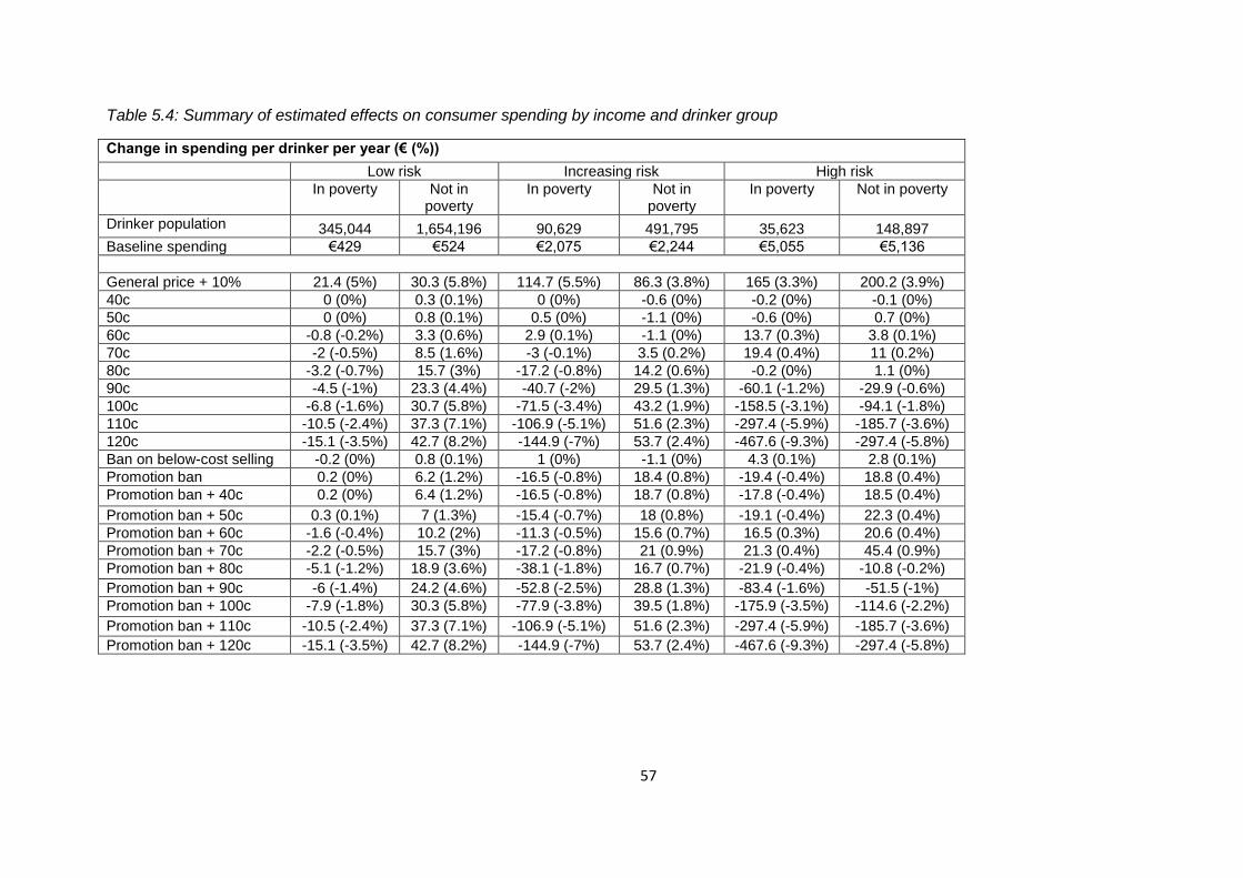
57
Table 5.4: Summary of estimated effects on consumer spending by income and drinker group
Change in spending per drinker per year (€ (%))
Low risk Increasing risk High risk
In poverty Not in poverty
In poverty Not in poverty
In poverty Not in poverty
Drinker population 345,044 1,654,196 90,629 491,795 35,623 148,897
Baseline spending €429 €524 €2,075 €2,244 €5,055 €5,136
General price + 10% 21.4 (5%) 30.3 (5.8%) 114.7 (5.5%) 86.3 (3.8%) 165 (3.3%) 200.2 (3.9%)
40c 0 (0%) 0.3 (0.1%) 0 (0%) -0.6 (0%) -0.2 (0%) -0.1 (0%)
50c 0 (0%) 0.8 (0.1%) 0.5 (0%) -1.1 (0%) -0.6 (0%) 0.7 (0%)
60c -0.8 (-0.2%) 3.3 (0.6%) 2.9 (0.1%) -1.1 (0%) 13.7 (0.3%) 3.8 (0.1%)
70c -2 (-0.5%) 8.5 (1.6%) -3 (-0.1%) 3.5 (0.2%) 19.4 (0.4%) 11 (0.2%)
80c -3.2 (-0.7%) 15.7 (3%) -17.2 (-0.8%) 14.2 (0.6%) -0.2 (0%) 1.1 (0%)
90c -4.5 (-1%) 23.3 (4.4%) -40.7 (-2%) 29.5 (1.3%) -60.1 (-1.2%) -29.9 (-0.6%)
100c -6.8 (-1.6%) 30.7 (5.8%) -71.5 (-3.4%) 43.2 (1.9%) -158.5 (-3.1%) -94.1 (-1.8%)
110c -10.5 (-2.4%) 37.3 (7.1%) -106.9 (-5.1%) 51.6 (2.3%) -297.4 (-5.9%) -185.7 (-3.6%)
120c -15.1 (-3.5%) 42.7 (8.2%) -144.9 (-7%) 53.7 (2.4%) -467.6 (-9.3%) -297.4 (-5.8%)
Ban on below-cost selling -0.2 (0%) 0.8 (0.1%) 1 (0%) -1.1 (0%) 4.3 (0.1%) 2.8 (0.1%)
Promotion ban 0.2 (0%) 6.2 (1.2%) -16.5 (-0.8%) 18.4 (0.8%) -19.4 (-0.4%) 18.8 (0.4%)
Promotion ban + 40c 0.2 (0%) 6.4 (1.2%) -16.5 (-0.8%) 18.7 (0.8%) -17.8 (-0.4%) 18.5 (0.4%)
Promotion ban + 50c 0.3 (0.1%) 7 (1.3%) -15.4 (-0.7%) 18 (0.8%) -19.1 (-0.4%) 22.3 (0.4%)
Promotion ban + 60c -1.6 (-0.4%) 10.2 (2%) -11.3 (-0.5%) 15.6 (0.7%) 16.5 (0.3%) 20.6 (0.4%)
Promotion ban + 70c -2.2 (-0.5%) 15.7 (3%) -17.2 (-0.8%) 21 (0.9%) 21.3 (0.4%) 45.4 (0.9%)
Promotion ban + 80c -5.1 (-1.2%) 18.9 (3.6%) -38.1 (-1.8%) 16.7 (0.7%) -21.9 (-0.4%) -10.8 (-0.2%)
Promotion ban + 90c -6 (-1.4%) 24.2 (4.6%) -52.8 (-2.5%) 28.8 (1.3%) -83.4 (-1.6%) -51.5 (-1%)
Promotion ban + 100c -7.9 (-1.8%) 30.3 (5.8%) -77.9 (-3.8%) 39.5 (1.8%) -175.9 (-3.5%) -114.6 (-2.2%)
Promotion ban + 110c -10.5 (-2.4%) 37.3 (7.1%) -106.9 (-5.1%) 51.6 (2.3%) -297.4 (-5.9%) -185.7 (-3.6%)
Promotion ban + 120c -15.1 (-3.5%) 42.7 (8.2%) -144.9 (-7%) 53.7 (2.4%) -467.6 (-9.3%) -297.4 (-5.8%)

58
Figure 5.5: Summary of relative spending changes by policy by drinker type
Figure 5.6: Summary of absolute spending changes by policy by drinker type
-10%
-8%
-6%
-4%
-2%
0%
2%
4%
6%
8%
10%
Re
lati
ve c
han
ge in
sp
en
din
g p
er
dri
nke
r
Low risk
Increasing risk
High risk
-400
-300
-200
-100
0
100
200
300
Ab
solu
te c
han
ge in
sp
en
din
g (€
pe
r d
rin
ker
pe
r ye
ar)
Low risk
Increasing risk
High risk

59
Figure 5.7: Income-specific effects of different levels of MUP on spending
5.1.3 Impact on retailers and the Exchequer
Table 5.5 shows the estimated impact of each policy on duty and VAT revenues to the exchequer as
well as the total revenue to retailers, separated between the on- and off-trades11.
11
Please also see note in Section 6.4 relating to VAT reclaims
-30%
-25%
-20%
-15%
-10%
-5%
0%
5%
10%
40c 50c 60c 70c 80c 90c 100c 110c 120c
Re
lati
ve c
han
ge in
sp
en
din
g p
er
dri
nke
r
Not in Poverty
In Poverty
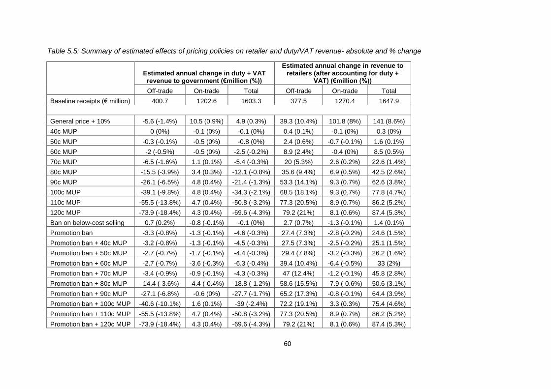
60
Table 5.5: Summary of estimated effects of pricing policies on retailer and duty/VAT revenue- absolute and % change
Estimated annual change in duty + VAT revenue to government (€million (%))
Estimated annual change in revenue to retailers (after accounting for duty +
VAT) (€million (%))
Off-trade On-trade Total Off-trade On-trade Total
Baseline receipts (€ million) 400.7 1202.6 1603.3 377.5 1270.4 1647.9
General price + 10% -5.6 (-1.4%) 10.5 (0.9%) 4.9 (0.3%) 39.3 (10.4%) 101.8 (8%) 141 (8.6%)
40c MUP 0 (0%) -0.1 (0%) -0.1 (0%) 0.4 (0.1%) -0.1 (0%) 0.3 (0%)
50c MUP -0.3 (-0.1%) -0.5 (0%) -0.8 (0%) 2.4 (0.6%) -0.7 (-0.1%) 1.6 (0.1%)
60c MUP -2 (-0.5%) -0.5 (0%) -2.5 (-0.2%) 8.9 (2.4%) -0.4 (0%) 8.5 (0.5%)
70c MUP -6.5 (-1.6%) 1.1 (0.1%) -5.4 (-0.3%) 20 (5.3%) 2.6 (0.2%) 22.6 (1.4%)
80c MUP -15.5 (-3.9%) 3.4 (0.3%) -12.1 (-0.8%) 35.6 (9.4%) 6.9 (0.5%) 42.5 (2.6%)
90c MUP -26.1 (-6.5%) 4.8 (0.4%) -21.4 (-1.3%) 53.3 (14.1%) 9.3 (0.7%) 62.6 (3.8%)
100c MUP -39.1 (-9.8%) 4.8 (0.4%) -34.3 (-2.1%) 68.5 (18.1%) 9.3 (0.7%) 77.8 (4.7%)
110c MUP -55.5 (-13.8%) 4.7 (0.4%) -50.8 (-3.2%) 77.3 (20.5%) 8.9 (0.7%) 86.2 (5.2%)
120c MUP -73.9 (-18.4%) 4.3 (0.4%) -69.6 (-4.3%) 79.2 (21%) 8.1 (0.6%) 87.4 (5.3%)
Ban on below-cost selling 0.7 (0.2%) -0.8 (-0.1%) -0.1 (0%) 2.7 (0.7%) -1.3 (-0.1%) 1.4 (0.1%)
Promotion ban -3.3 (-0.8%) -1.3 (-0.1%) -4.6 (-0.3%) 27.4 (7.3%) -2.8 (-0.2%) 24.6 (1.5%)
Promotion ban + 40c MUP -3.2 (-0.8%) -1.3 (-0.1%) -4.5 (-0.3%) 27.5 (7.3%) -2.5 (-0.2%) 25.1 (1.5%)
Promotion ban + 50c MUP -2.7 (-0.7%) -1.7 (-0.1%) -4.4 (-0.3%) 29.4 (7.8%) -3.2 (-0.3%) 26.2 (1.6%)
Promotion ban + 60c MUP -2.7 (-0.7%) -3.6 (-0.3%) -6.3 (-0.4%) 39.4 (10.4%) -6.4 (-0.5%) 33 (2%)
Promotion ban + 70c MUP -3.4 (-0.9%) -0.9 (-0.1%) -4.3 (-0.3%) 47 (12.4%) -1.2 (-0.1%) 45.8 (2.8%)
Promotion ban + 80c MUP -14.4 (-3.6%) -4.4 (-0.4%) -18.8 (-1.2%) 58.6 (15.5%) -7.9 (-0.6%) 50.6 (3.1%)
Promotion ban + 90c MUP -27.1 (-6.8%) -0.6 (0%) -27.7 (-1.7%) 65.2 (17.3%) -0.8 (-0.1%) 64.4 (3.9%)
Promotion ban + 100c MUP -40.6 (-10.1%) 1.6 (0.1%) -39 (-2.4%) 72.2 (19.1%) 3.3 (0.3%) 75.4 (4.6%)
Promotion ban + 110c MUP -55.5 (-13.8%) 4.7 (0.4%) -50.8 (-3.2%) 77.3 (20.5%) 8.9 (0.7%) 86.2 (5.2%)
Promotion ban + 120c MUP -73.9 (-18.4%) 4.3 (0.4%) -69.6 (-4.3%) 79.2 (21%) 8.1 (0.6%) 87.4 (5.3%)

61
5.1.4 Impact on health outcomes
Table 5.6 presents the impact of each modelled policy on deaths and hospital admissions per year at
full effect (i.e. in the 20th year following policy implementation) as well as the estimated annual QALY
gains. These are shown as relative changes in Figure 5.8. Table 5.7 illustrates the equity implications
of the health impact of each policy by showing the reductions in deaths and hospitalisations at full
effect for each income group. These figures are illustrated graphically in Figure 5.9 and Figure 5.10.
Table 5.8 shows the impact of each policy at full effect on liver disease outcomes. Table 5.9 and
Table 5.10 present the ‘partial effects’ of each policy on deaths and hospital admissions – i.e. the
changing impact across the 20 years following policy implementation – broken down by condition
type. Figure 5.11 and Figure 5.12 show these trends over time in total deaths and hospital
admissions.
The principal finding is that both MUP and promotion ban policies are effective at improving alcohol-
related health outcomes, with a 90c MUP estimated to lead to a 10.9% reduction in alcohol-related
deaths and 7.0% fewer alcohol-related hospital admissions per year (in the 20th year following policy
implementation when the full effect of the health benefits of the policy are felt). The majority of
these gains (66.2% of deaths and 64.8% of admissions for a 90c MUP) are in improved chronic
disease outcomes, particularly alcoholic liver disease (29.5% of all deaths and 11.0% of all admissions
for a 90c MUP). Higher MUP thresholds lead to greater health benefits (e.g. a 15.5% reduction in
deaths and 10.0% reduction in hospital admissions for 100c MUP), as does the addition of a ban on
off-trade promotions to an MUP policy (e.g. a 12.9% and 8.36% reduction in deaths and hospital
admissions respectively for a 90c MUP policy combined with a promotions ban).

62
Table 5.6: Summary of policy impacts on health outcomes – changes in alcohol-related deaths, hospital admissions and QALYs per year at full effect (20 years)
Policy
Estimated change in deaths in 20th year
following policy implementation
Estimated change in hospital admissions in 20th
year following policy implementation
Estimated QALYs gained in
20th year following policy implementation Total Acute Chronic Total Acute Chronic
Baseline level 1,270 740 530 58,961 24,499 34,462
General price + 10% -147 -58 -89 -4,666 -1,870 -2,797 1,184
40c MUP -1 0 -1 -46 -6 -40 8
50c MUP -6 -1 -4 -206 -46 -160 45
60c MUP -23 -7 -16 -674 -196 -478 173
70c MUP -46 -14 -32 -1,338 -427 -912 365
80c MUP -88 -29 -59 -2,549 -879 -1,670 708
90c MUP -139 -47 -92 -4,102 -1,443 -2,659 1,130
100c MUP -197 -68 -129 -5,878 -2,086 -3,792 1,603
110c MUP -257 -89 -168 -7,737 -2,770 -4,967 2,098
120c MUP -312 -111 -202 -9,483 -3,434 -6,048 2,561
Ban on below-cost selling
-4 -1 -3 -166 -27 -139 31
Promotion ban -45 -15 -30 -1,382 -486 -896 361
Promotion ban + 40c MUP
-46 -16 -30 -1,403 -488 -915 365
Promotion ban + 50c MUP
-46 -15 -31 -1,445 -482 -963 370
Promotion ban + 60c MUP
-65 -21 -44 -1,992 -640 -1,352 510
Promotion ban + 70c MUP
-73 -22 -51 -2,164 -676 -1,488 571
Promotion ban + 80c MUP
-121 -40 -81 -3,595 -1,237 -2,358 969
Promotion ban + 90c MUP
-164 -56 -108 -4,896 -1,722 -3,174 1,326
Promotion ban + 100c MUP
-210 -72 -137 -6,294 -2,241 -4,053 1,708
Promotion ban + 110c MUP
-257 -89 -168 -7,737 -2,770 -4,967 2,098
Promotion ban + 120c MUP
-312 -111 -202 -9,483 -3,434 -6,048 2,561

63
Table 5.7: Income specific health outcomes – policy impacts on deaths and hospital admissions per year per 100,000 population at full effect (20 years)
Policy
In poverty Not in poverty
Deaths per 100,000
population
Hospital admissions per
100,000 population
Deaths per 100,000
population
Hospital admissions per
100,000 population
Baseline 46.5 1961.9 33.3 1589.9
General price + 10% -3.4 -110.6 -4.3 -136.2
40c MUP 0.0 -0.1 0.0 -1.6
50c MUP 0.0 -1.8 -0.2 -6.7
60c MUP -0.3 -12.2 -0.7 -20.6
70c MUP -1.2 -40.8 -1.3 -37.0
80c MUP -2.6 -89.5 -2.4 -67.7
90c MUP -4.4 -153.9 -3.8 -106.6
100c MUP -6.2 -227.1 -5.4 -151.2
110c MUP -8.1 -298.2 -7.0 -199.1
120c MUP -9.9 -364.7 -8.5 -244.3
Ban on below-cost selling 0.0 -0.6 -0.1 -5.6
Promotion ban -1.2 -44.3 -1.3 -37.7
Promotion ban + 40c MUP -1.2 -43.9 -1.3 -38.5
Promotion ban + 50c MUP -1.2 -43.7 -1.3 -40.0
Promotion ban + 60c MUP -1.4 -51.3 -1.9 -57.2
Promotion ban + 70c MUP -1.8 -64.6 -2.1 -60.1
Promotion ban + 80c MUP -3.4 -118.5 -3.4 -97.2
Promotion ban + 90c MUP -4.8 -175.3 -4.6 -129.1
Promotion ban + 100c MUP -6.5 -237.5 -5.8 -163.2
Promotion ban + 110c MUP -8.1 -298.2 -7.0 -199.1
Promotion ban + 120c MUP -9.9 -364.7 -8.5 -244.3

64
Figure 5.8: Summary of relative changes in deaths and hospital admissions per year at full effect
Figure 5.9: Income-specific reductions in deaths per year per 100,000 population
-30%
-25%
-20%
-15%
-10%
-5%
0%
5%
10%
Ch
ange
in h
eal
th h
arm
vo
lum
es
pe
r ye
ar
Deaths
Hospitaladmissions
-12
-10
-8
-6
-4
-2
0
Re
du
ctio
ns
in d
eat
hs
pe
r ye
ar p
er
10
0,0
00
p
op
ula
tio
n
In poverty
Not in poverty

65
Figure 5.10: Income-specific reductions in hospital admissions per year per 100,000 population
-400
-350
-300
-250
-200
-150
-100
-50
0
Re
du
ctio
n in
ho
spit
al a
dm
issi
on
s p
er
10
0,0
00
p
op
ula
tio
n p
er
year
In poverty
Not in poverty

66
Table 5.8: Summary of policy impacts on alcoholic liver disease outcomes at full effect (20 years)
Policy Alcoholic liver disease (ICD-10 code K70)
Deaths Hospital admissions
Baseline 340 3,602
General price + 10% -37 -390
40c MUP 0 -4
50c MUP -2 -20
60c MUP -7 -78
70c MUP -15 -160
80c MUP -27 -293
90c MUP -41 -450
100c MUP -57 -621
110c MUP -73 -801
120c MUP -89 -968
Ban on below-cost selling -1 -13
Promotion ban -13 -141
Promotion ban + 40c MUP -13 -143
Promotion ban + 50c MUP -14 -146
Promotion ban + 60c MUP -19 -209
Promotion ban + 70c MUP -22 -241
Promotion ban + 80c MUP -36 -387
Promotion ban + 90c MUP -48 -518
Promotion ban + 100c MUP -60 -657
Promotion ban + 110c MUP -73 -801
Promotion ban + 120c MUP -89 -968

67
Table 5.9: Summary of impact of policies on annual deaths by condition type
Policy
Reduction in deaths per year - partial effects
Acute Chronic Total
Year 1
Year 5
Year 10
Year 15
Year 20
Year 1
Year 5
Year 10
Year 15
Year 20
Year 1
Year 5
Year 10
Year 15
Year 20
Baseline 626 671 708 728 740 -6*
-30*
41 307 530 619 641 750 1,035 1,270
General price +10% -51 -54 -56 -57 -58 -12 -38 -52 -72 -89 -63 -92 -108 -130 -147
40c MUP 0 0 0 0 0 0 0 -1 -1 -1 0 -1 -1 -1 -1
50c MUP -1 -1 -1 -1 -1 0 -2 -2 -3 -4 -2 -3 -4 -5 -6
60c MUP -5 -6 -6 -6 -7 -2 -6 -9 -13 -16 -7 -12 -16 -19 -23
70c MUP -12 -13 -14 -14 -14 -3 -12 -18 -26 -32 -15 -26 -32 -40 -46
80c MUP -26 -28 -29 -29 -29 -6 -23 -34 -48 -59 -32 -51 -63 -77 -88
90c MUP -42 -45 -47 -47 -47 -10 -38 -54 -75 -92 -52 -83 -101 -122 -139
100c MUP -61 -65 -68 -68 -68 -14 -53 -76 -105 -129 -75 -118 -143 -173 -197
110c MUP -81 -86 -90 -90 -89 -19 -69 -98 -136 -168 -100 -155 -187 -226 -257
120c MUP -101 -107 -111 -111 -111 -23 -83 -117 -164 -202 -124 -190 -228 -275 -312
Ban on below-cost selling 0 -1 -1 -1 -1 0 -1 -2 -3 -3 -1 -2 -3 -3 -4
Promotion ban -13 -14 -15 -15 -15 -4 -12 -18 -24 -30 -17 -27 -33 -40 -45
Promotion ban + 40c MUP -13 -15 -15 -16 -16 -4 -13 -18 -25 -30 -17 -27 -33 -40 -46
Promotion ban + 50c MUP -13 -14 -15 -15 -15 -4 -13 -18 -25 -31 -17 -27 -33 -41 -46
Promotion ban + 60c MUP -17 -19 -20 -21 -21 -5 -18 -26 -36 -44 -22 -37 -46 -57 -65
Promotion ban + 70c MUP -19 -21 -22 -22 -22 -6 -21 -30 -41 -51 -24 -41 -52 -64 -73
Promotion ban + 80c MUP -36 -38 -40 -40 -40 -9 -33 -47 -65 -81 -44 -71 -87 -105 -121
Promotion ban + 90c MUP -50 -53 -56 -56 -56 -12 -44 -63 -88 -108 -62 -98 -119 -144 -164
Promotion ban + 100c MUP
-65 -69 -72 -73 -72 -15 -57 -80 -112 -137 -81 -126 -153 -184 -210
Promotion ban + 110c MUP
-81 -86 -90 -90 -89 -19 -69 -98 -136 -168 -100 -155 -187 -226 -257
Promotion ban + 120c MUP
-101 -107 -111 -111 -111 -23 -83 -117 -164 -202 -124 -190 -228 -275 -312
* This value is negative because it is estimated that, due to the ‘protective’ effect of moderate alcohol consumption on ischaemic heart disease, ischaemic stroke and type II diabetes, alcohol has an overall
protective effect for low risk drinkers, although there is some debate in the scientific community that this effect exists at all (see, for example [38])
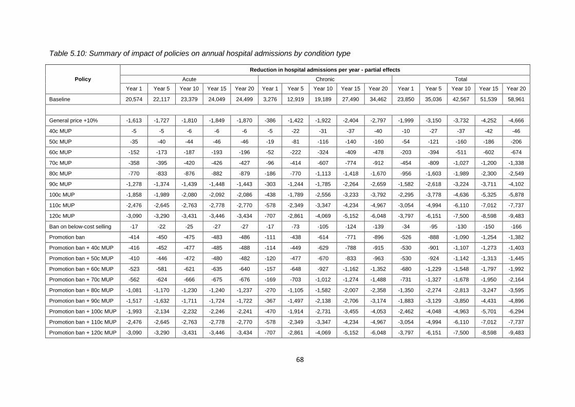
68
Table 5.10: Summary of impact of policies on annual hospital admissions by condition type
Policy
Reduction in hospital admissions per year - partial effects
Acute Chronic Total
Year 1 Year 5 Year 10 Year 15 Year 20 Year 1 Year 5 Year 10 Year 15 Year 20 Year 1 Year 5 Year 10 Year 15 Year 20
Baseline 20,574 22,117 23,379 24,049 24,499 3,276 12,919 19,189 27,490 34,462 23,850 35,036 42,567 51,539 58,961
General price +10% -1,613 -1,727 -1,810 -1,849 -1,870 -386 -1,422 -1,922 -2,404 -2,797 -1,999 -3,150 -3,732 -4,252 -4,666
40c MUP -5 -5 -6 -6 -6 -5 -22 -31 -37 -40 -10 -27 -37 -42 -46
50c MUP -35 -40 -44 -46 -46 -19 -81 -116 -140 -160 -54 -121 -160 -186 -206
60c MUP -152 -173 -187 -193 -196 -52 -222 -324 -409 -478 -203 -394 -511 -602 -674
70c MUP -358 -395 -420 -426 -427 -96 -414 -607 -774 -912 -454 -809 -1,027 -1,200 -1,338
80c MUP -770 -833 -876 -882 -879 -186 -770 -1,113 -1,418 -1,670 -956 -1,603 -1,989 -2,300 -2,549
90c MUP -1,278 -1,374 -1,439 -1,448 -1,443 -303 -1,244 -1,785 -2,264 -2,659 -1,582 -2,618 -3,224 -3,711 -4,102
100c MUP -1,858 -1,989 -2,080 -2,092 -2,086 -438 -1,789 -2,556 -3,233 -3,792 -2,295 -3,778 -4,636 -5,325 -5,878
110c MUP -2,476 -2,645 -2,763 -2,778 -2,770 -578 -2,349 -3,347 -4,234 -4,967 -3,054 -4,994 -6,110 -7,012 -7,737
120c MUP -3,090 -3,290 -3,431 -3,446 -3,434 -707 -2,861 -4,069 -5,152 -6,048 -3,797 -6,151 -7,500 -8,598 -9,483
Ban on below-cost selling -17 -22 -25 -27 -27 -17 -73 -105 -124 -139 -34 -95 -130 -150 -166
Promotion ban -414 -450 -475 -483 -486 -111 -438 -614 -771 -896 -526 -888 -1,090 -1,254 -1,382
Promotion ban + 40c MUP -416 -452 -477 -485 -488 -114 -449 -629 -788 -915 -530 -901 -1,107 -1,273 -1,403
Promotion ban + 50c MUP -410 -446 -472 -480 -482 -120 -477 -670 -833 -963 -530 -924 -1,142 -1,313 -1,445
Promotion ban + 60c MUP -523 -581 -621 -635 -640 -157 -648 -927 -1,162 -1,352 -680 -1,229 -1,548 -1,797 -1,992
Promotion ban + 70c MUP -562 -624 -666 -675 -676 -169 -703 -1,012 -1,274 -1,488 -731 -1,327 -1,678 -1,950 -2,164
Promotion ban + 80c MUP -1,081 -1,170 -1,230 -1,240 -1,237 -270 -1,105 -1,582 -2,007 -2,358 -1,350 -2,274 -2,813 -3,247 -3,595
Promotion ban + 90c MUP -1,517 -1,632 -1,711 -1,724 -1,722 -367 -1,497 -2,138 -2,706 -3,174 -1,883 -3,129 -3,850 -4,431 -4,896
Promotion ban + 100c MUP -1,993 -2,134 -2,232 -2,246 -2,241 -470 -1,914 -2,731 -3,455 -4,053 -2,462 -4,048 -4,963 -5,701 -6,294
Promotion ban + 110c MUP -2,476 -2,645 -2,763 -2,778 -2,770 -578 -2,349 -3,347 -4,234 -4,967 -3,054 -4,994 -6,110 -7,012 -7,737
Promotion ban + 120c MUP -3,090 -3,290 -3,431 -3,446 -3,434 -707 -2,861 -4,069 -5,152 -6,048 -3,797 -6,151 -7,500 -8,598 -9,483

69
Figure 5.11: Estimated reductions in deaths over time for exemplar MUP policies
Figure 5.12: Estimated reductions in hospital admissions over time for exemplar MUP policies
-250
-200
-150
-100
-50
0
0 5 10 15 20
Nu
mb
er
of
de
ath
s av
ert
ed
pe
r ye
ar
Years since policy implementation
90c MUP
100c MUP
-7000
-6000
-5000
-4000
-3000
-2000
-1000
0
0 5 10 15 20
Nu
mb
er
of
ho
spit
al a
dm
issi
on
s av
ert
ed
pe
r ye
ar
Years since policy implementation
90c MUP
100c MUP

70
5.1.5 Impact on crime outcomes
The estimated impact of the modelled policies on annual volumes of crime is shown in Table 5.11,
including the differential impact by drinker group. Table 5.12 shows the changes in annual crime
volumes, broken down further by category of crime. Relative reductions in crime by drinker group
are presented in Figure 5.13.
The principal finding is that MUP policies, a ban on off-trade promotions and combinations of the
two are effective measures to reduce alcohol-related crime. A 90c MUP policy is estimated to lead to
1,043 fewer alcohol-related crimes per year, a reduction of 5.3%. The majority of these gains (70.5%
for a 90c MUP) are from reduced levels of criminal damage. Higher MUP thresholds lead to greater
reductions (e.g. 1,493 fewer crimes for a 100c MUP) as does the addition of a promotions ban to an
MUP policy (e.g. 1,182 fewer crimes for a 90c MUP in combination with a promotions ban.

71
Table 5.11: Impact of modelled policies on annual crime volumes
Policy Changes in annual crime volumes
Population Low risk Increasing
risk High risk
Baseline volume 19,844 8,592 6,977 4,275
General price + 10% -1,002 -486 -330 -186
40c MUP -2 -1 0 0
50c MUP -26 -9 -6 -11
60c MUP -121 -39 -41 -41
70c MUP -317 -86 -124 -107
80c MUP -654 -183 -256 -215
90c MUP -1,043 -306 -396 -341
100c MUP -1,493 -461 -547 -485
110c MUP -1,973 -638 -698 -637
120c MUP -2,453 -819 -845 -788
Ban on below-cost selling -3 -2 -1 0
Promotion ban -271 -85 -92 -95
Promotion ban + 40c MUP -269 -86 -91 -92
Promotion ban + 50c MUP -262 -76 -85 -101
Promotion ban + 60c MUP -325 -94 -110 -122
Promotion ban + 70c MUP -385 -89 -158 -138
Promotion ban + 80c MUP -849 -252 -329 -269
Promotion ban + 90c MUP -1,182 -364 -438 -380
Promotion ban + 100c MUP -1,582 -501 -573 -508
Promotion ban + 110c MUP -1,973 -638 -698 -637
Promotion ban + 120c MUP -2,453 -819 -845 -788

72
Table 5.12: Estimated changes in annual crime volumes by crime category
Policy
Changes in annual crime volumes
Violent crimes
Criminal damage
Robbery, burglary & theft
Baseline volume 4,101 13,460 2,283
General price + 10% -210 -689 -103
40c MUP 0 -1 0
50c MUP -5 -18 -2
60c MUP -23 -87 -11
70c MUP -60 -226 -31
80c MUP -125 -463 -67
90c MUP -200 -735 -108
100c MUP -288 -1,048 -157
110c MUP -381 -1,382 -209
120c MUP -475 -1,717 -261
Ban on below-cost selling -1 -2 0
Promotion ban -55 -189 -27
Promotion ban + 40c MUP -54 -188 -27
Promotion ban + 50c MUP -53 -183 -26
Promotion ban + 60c MUP -64 -230 -31
Promotion ban + 70c MUP -75 -273 -37
Promotion ban + 80c MUP -165 -596 -88
Promotion ban + 90c MUP -229 -830 -123
Promotion ban + 100c MUP -306 -1,110 -167
Promotion ban + 110c MUP -381 -1,382 -209
Promotion ban + 120c MUP -475 -1,717 -261
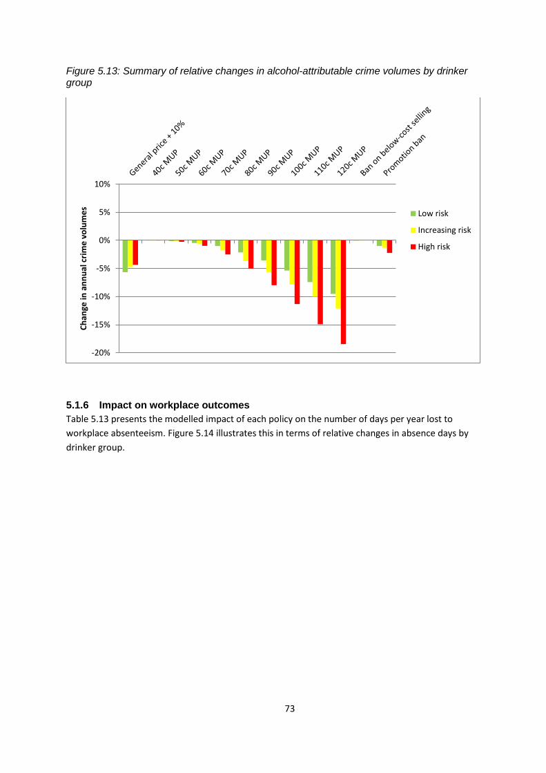
73
Figure 5.13: Summary of relative changes in alcohol-attributable crime volumes by drinker group
5.1.6 Impact on workplace outcomes
Table 5.13 presents the modelled impact of each policy on the number of days per year lost to
workplace absenteeism. Figure 5.14 illustrates this in terms of relative changes in absence days by
drinker group.
-20%
-15%
-10%
-5%
0%
5%
10%
Ch
ange
in a
nn
ual
cri
me
vo
lum
es
Low risk
Increasing risk
High risk

74
Table 5.13: Estimated changes in workplace absence
Policy Changes in days absence from work (1,000s)
Population Low risk Increasing
risk High risk
Baseline absence 1106.6 434.3 413.8 258.5
General price + 10% -82.7 -37.9 -28.2 -16.6
40c MUP -0.5 0.0 -0.2 -0.3
50c MUP -2.2 -0.4 -0.7 -1.1
60c MUP -7.6 -1.4 -2.9 -3.3
70c MUP -20.0 -3.9 -7.6 -8.5
80c MUP -45.3 -10.9 -16.9 -17.5
90c MUP -77.8 -21.0 -28.8 -28.1
100c MUP -115.6 -33.2 -42.3 -40.1
110c MUP -155.9 -46.9 -56.2 -52.9
120c MUP -197.1 -61.0 -70.3 -65.8
Ban on below-cost selling -0.9 0.1 -0.4 -0.6
Promotion ban -21.4 -6.4 -7.8 -7.1
Promotion ban + 40c MUP -21.4 -6.4 -7.9 -7.1
Promotion ban + 50c MUP -21.5 -5.9 -7.7 -7.9
Promotion ban + 60c MUP -25.6 -5.8 -10.0 -9.9
Promotion ban + 70c MUP -28.9 -5.0 -12.1 -11.8
Promotion ban + 80c MUP -63.9 -16.8 -24.0 -23.1
Promotion ban + 90c MUP -91.1 -25.8 -33.7 -31.7
Promotion ban + 100c MUP -123.6 -36.4 -45.0 -42.2
Promotion ban + 110c MUP -155.9 -46.9 -56.2 -52.9
Promotion ban + 120c MUP -197.1 -61.0 -70.3 -65.8

75
Figure 5.14: Summary of relative changes in workplace absence by drinker
5.1.7 Impact on societal costs
Table 5.14 gives an overview of the estimated annual savings resulting from the implementation of
each of the modelled policies. These savings are presented separately for healthcare costs, costs
associated with crime and the cost of workplace absenteeism. It should be noted that these costs
may not be fully realised in practice as, for example, crime costs incorporate a financial valuation of
the impact on the victim.
-30%
-25%
-20%
-15%
-10%
-5%
0%
5%
10%
Ch
ange
in w
ork
pla
ce a
bse
nce
s p
er
year
Low risk
Increasing risk
High risk

76
Table 5.14: Summary of financial valuation of impact of modelled policies on health, crime and workplace related harm in year 1 and cumulatively over 20 years
Policy
Value of harm reductions in year 1 (€m)
Cumulative value of harm reductions over 20 years (€m)
Healthcare costs
QALY valuation
Crime costs
Work absence
costs
Total costs
Healthcare costs
QALY valuation
Crime costs
Work absence
costs
Total costs
Baseline cost (€millions) 78.6
98.1 149.4 326.1
2,301.7
1,442.9 2,198.4 5,943.0
General price + 10% -5.7 -21.8 -5.2 -12.3 -45.0
-186.9 -852.4 -76.3 -180.3 -1,295.9
40c MUP 0.0 -0.1 0.0 -0.1 -0.2
-2.4 -5.7 -0.1 -1.2 -9.3
50c MUP -0.2 -0.6 -0.1 -0.3 -1.2
-9.5 -30.0 -1.9 -5.0 -46.4
60c MUP -0.7 -2.2 -0.6 -1.2 -4.7
-29.1 -113.2 -8.6 -17.4 -168.4
70c MUP -1.5 -5.1 -1.5 -2.9 -11.0
-58.3 -242.7 -21.5 -42.4 -364.9
80c MUP -3.1 -10.9 -3.0 -6.4 -23.4
-110.9 -480.4 -44.8 -93.6 -729.7
90c MUP -5.2 -17.9 -4.9 -10.9 -38.8
-178.1 -774.7 -71.6 -160.3 -1,184.7
100c MUP -7.4 -25.9 -7.0 -16.1 -56.5
-254.7 -1,106.5 -102.7 -236.6 -1,700.5
110c MUP -9.9 -34.5 -9.2 -21.7 -75.3
-334.6 -1,454.3 -136.0 -318.7 -2,243.6
120c MUP -12.3 -42.9 -11.5 -27.4 -94.1
-409.6 -1,784.4 -169.0 -402.7 -2,765.8
Ban on below-cost selling -0.1 -0.3 0.0 -0.2 -0.6
-7.9 -20.8 -0.4 -2.3 -31.4
Promotion ban -1.6 -5.8 -1.4 -3.2 -11.9
-58.7 -249.8 -20.0 -46.8 -375.3
Promotion ban + 40c MUP -1.6 -5.8 -1.3 -3.2 -12.0
-59.8 -252.4 -19.8 -47.1 -379.1
Promotion ban + 50c MUP -1.7 -5.8 -1.3 -3.2 -12.0
-62.5 -255.1 -19.2 -47.7 -384.6
Promotion ban + 60c MUP -2.2 -7.4 -1.6 -4.1 -15.3
-85.7 -345.1 -23.5 -59.6 -513.9
Promotion ban + 70c MUP -2.4 -8.1 -1.8 -4.4 -16.7
-94.6 -383.0 -27.1 -64.1 -568.7
Promotion ban + 80c MUP -4.4 -15.2 -4.0 -8.9 -32.5 -156.1 -663.7 -59.4 -130.3 -1,009.4
Promotion ban + 90c MUP -6.1 -21.2 -5.6 -12.9 -45.7 -211.6 -912.8 -81.9 -189.1 -1,395.5
Promotion ban + 100c MUP -8.0 -37.1 -7.4 -17.2 -69.7 -272.1 -1,180.6 -109.3 -253.3 -1,815.3
Promotion ban + 110c MUP -9.9 -34.5 -9.2 -21.7 -75.3 -334.6 -1,454.3 -136.0 -318.7 -2,243.6
Promotion ban + 120c MUP -12.3 -21.8 -11.5 -27.4 -94.1 -409.6 -1,784.4 -169.0 -402.7 -2765.8

77
5.2 EXAMPLE POLICY ANALYSIS A: 90C MUP
This section describes the estimated impacts of a minimum unit price policy of 90c per standard
drink in detail. We assume that this threshold is updated annually in line with inflation. In addition to
the results already presented in Table 5.1 to Table 5.14, further detailed results are shown in Table
5.15 to Table 5.19 and in Figure 5.15 for consumption changes, consumer spending and health
outcomes.
Across the whole population, 34.3% of standard drinks purchased would be affected (i.e. would
have their price raised to 90c). The proportion and absolute number of purchased standard drinks
per week affected for high risk drinkers (44.5% or 27.8 std. drinks) is substantially more than for
increasing risk drinkers (32.4% or 7.1 std. drinks) or low risk drinkers (29.6% or 1.0 std. drink). The
proportion and number of purchased standard drinks per week affected is slightly higher for those in
poverty than those above the poverty line (38.4% and 3.4 std. drinks vs. 33.3% and 3.2 std. drinks),
though this difference is primarily driven by a substantial difference between high risk drinkers in
poverty (54.8% or 41.3 std. drinks) vs. high risk drinkers not in poverty (41.6% or 24.8 std. drinks).
Across the whole population, mean weekly consumption is estimated to change by -6.2%.
Consumption is estimated to reduce by 0.58 std. drinks per person, or 0.74 std. drinks per drinker
per week. Weekly consumption reductions are greater for high risk drinkers (-9.4% or 6.7 std. drinks)
than low risk drinkers (-1.9% or 0.1 std. drinks) and for those in poverty (-8.7% or 1.1 std. drinks)
compared to those not in poverty (-5.6% or 0.7 std. drinks).
In both income groups, absolute reductions in consumption are estimated to be small for low risk
drinkers and much larger for high risk drinkers. However; for people below the poverty line the
relative change in consumption is similar across all drinkers, while for those above the poverty line
the relative changes are considerably larger for heavier drinkers. The estimated consumption
reduction for low risk drinkers in poverty is -8.6% or 0.35 std. drinks per week compared to -9.8% or
7.34 std. drinks per week for high risk drinkers in poverty. The corresponding figures for those not in
poverty are -0.6% or 0.03 std. drinks and -11.0% or 6.57 std. drinks.
Across the whole population, estimated spending increases by 1.3% or €14.90 per drinker per year
(€0.29 per week). The cost impact of the policy on consumer spending varies significantly between
different drinker and income subgroups. Low risk and increasing risk drinkers are estimated to
increase their spending by €18.50 and €18.60 per year respectively, while high risk drinkers reduce
their spending by €35.80. Similar differences are observed between income subgroups, with those in
poverty saving €15.70 per year compared to a spending increase of €21.20 per year for those not in
poverty.
Those in poverty are estimated to save money at all levels of consumption, with low risk,
increasing risk and high risk drinkers saving €4.50, €40.70 and €60.10 per year respectively. A
different pattern is observed for those not in poverty, with low risk and increasing risk drinkers
increasing their spending by €23.30 and €29.50 per year respectively, whilst high risk drinkers reduce
their spending by €29.90. These differing patterns are a result of both the different proportion of
each population subgroup’s purchases which are affected by the policy, as well as the different price

78
elasticities of the beverages which make up a greater or lesser proportion of each subgroup’s
purchases.
Overall revenue to the Exchequer from duty and VAT receipts is estimated to reduce by 1.3% or
€21.4 million12.
Revenue to retailers is estimated to increase by €53.3million (14.1%) in the off-trade and
€9.3million (0.7%) in the on-trade. This is as reduced sales volumes are more than offset by the
increased value of remaining sales.
Effects on health are estimated to be substantial, with alcohol-attributable deaths estimated to
reduce by approximately 139 per year after 20 years, by which time the full effects of the policy will
be seen. Annual deaths are distributed differentially across drinker groups with approximately 7
saved amongst low risk drinkers, 40 amongst increasing risk drinkers and 92 amongst high risk
drinkers. Whilst those in poverty see a smaller absolute number of reduced deaths (29 vs. 110 for
those not in poverty), they also comprise a substantially smaller proportion of the population
(18.9%), meaning that the relative reductions in annual deaths per 100,000 population is greater
amongst those in poverty (4.4 vs. 3.8 per 100,000 for those not in poverty).
Similar patterns are observed amongst reductions in alcohol-related hospital admissions, with an
estimated 4,102 fewer admissions per year across the population. Admissions reductions for low
risk, increasing risk and high risk drinkers are 330, 1,180 and 2,590 respectively. Again, those in
poverty experience a lower absolute reduction in hospital admissions (1,030 vs. 3,070) but a larger
reduction per 100,000 population (154 vs. 107). Direct healthcare costs are estimated to reduce by
€5.2m in year 1 and by €178.1m cumulatively over 20 years.
Crime is estimated to fall by 1,043 offences per year overall. Reductions are spread relatively
evenly between drinker groups, with 306, 396 and 341 fewer offences committed by low risk,
increasing risk and high risk drinkers respectively. However, it should be noted that increasing risk
and high risk drinkers (16% and 5% respectively) make up a considerably smaller proportion of the
population than low risk drinkers (78%). Costs of crime and policing are estimated to reduce by
€4.9m in year 1 and by €71.6m cumulatively over 20 years.
Workplace absence is estimated to be reduced by 77,800 per year. This is estimated to lead to an
annual saving of €10.9m in year 1 and €160.3m over 20 years.
The total societal value of these reductions in health, crime and workplace harms is estimated at
€1.18bn over the 20 year period modelled. This includes direct healthcare costs (€178m), crime
costs (€72m), workplace costs (€160m) and a financial valuation of the QALY gain (€775m), assuming
a QALY is valued at €45,000. All costs and benefits are discounted at 3.5%.
12
Please also see note in Section 6.4 on VAT reclaims
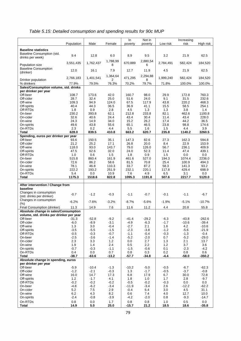
79
Table 5.15: Detailed consumption and spending results for 90c MUP
Population Male Female In
poverty Not in
poverty Low risk Increasing
risk High risk
Baseline statistics Baseline Consumption (std. drinks per week)
9.4 12.8 6.0 8.9 9.5 3.2 21.9 62.5
Population size 3,551,435 1,762,437
1,788,998
670,889 2,880,54
6 2,784,491 582,424 184,520
Baseline Consumption (drinker)
12.0 16.1 7.9 12.7 11.9 4.5 21.9 62.5
Drinker population 2,766,183 1,401,541
1,364,642
471,295 2,294,88
8 1,999,240 582,424 184,520
% drinkers 77.9% 79.5% 76.3% 70.2% 79.7% 71.8% 100.0% 100.0%
Sales/Consumption volume, std. drinks per drinker per year
Off-beer 108.7 173.6 42.0 160.7 98.0 29.9 172.8 760.3 Off-cider 28.7 32.4 25.0 51.6 24.0 9.1 31.5 232.6 Off-wine 109.3 94.9 124.0 67.5 117.9 43.8 220.2 468.3 Off-spirits 40.4 44.3 36.5 36.9 41.1 15.5 58.5 254.1 Off-RTDs 1.8 0.9 2.8 4.5 1.3 1.3 3.8 1.4 On-beer 230.2 393.8 62.1 212.8 233.8 82.1 462.6 1100.8 On-cider 32.6 40.6 24.4 43.4 30.4 11.4 43.4 228.0 On-wine 24.3 14.9 34.0 15.2 26.2 17.4 44.2 36.5 On-spirits 49.6 43.8 55.6 65.1 46.5 23.8 98.8 174.6 On-RTDs 2.3 0.2 4.4 5.5 1.6 1.5 4.4 3.9 Total 628.0 839.5 410.8 663.2 620.7 235.8 1140.2 3260.5
Spending, euros per drinker per year Off-beer 93.6 150.5 35.1 147.3 82.6 27.3 162.3 594.8
Off-cider 21.2 25.2 17.1 26.8 20.0 8.4 22.9 153.9 Off-wine 118.0 93.0 143.7 79.0 126.0 56.7 236.1 409.9 Off-spirits 47.5 62.6 32.0 24.0 52.3 11.4 47.4 439.1 Off-RTDs 1.0 0.6 1.5 1.8 0.9 1.5 0.0 0.0 On-beer 515.8 860.4 161.9 461.6 527.0 194.3 1074.4 2236.0 On-cider 72.6 86.2 58.6 81.5 70.8 25.4 100.9 494.3 On-wine 78.1 46.8 110.3 33.7 87.2 58.3 141.3 93.2 On-spirits 222.2 193.2 251.9 232.1 220.1 117.8 429.4 698.9 On-RTDs 5.4 0.0 10.9 7.6 4.9 6.5 3.1 0.0 Total 1175.3 1518.6 822.8 1095.3 1191.8 507.6 2217.7 5120.0
After intervention / Change from
baseline Changes in consumption
(std. drinks per drinker) -0.7 -1.2 -0.3 -1.1 -0.7 -0.1 -1.1 -6.7
Changes in consumption (%)
-6.2% -7.6% -3.2% -8.7% -5.6% -1.9% -5.1% -10.7%
Final Consumption (drinker) 11.3 14.9 7.6 11.6 11.2 4.4 20.8 55.8
Absolute change in sales/Consumption volume, std. drinks per drinker per year
Off-beer -31.3 -52.8 -9.2 -41.4 -29.2 -6.3 -43.8 -262.6 Off-cider -6.0 -8.9 -3.1 -4.9 -6.3 -1.7 -10.6 -39.4 Off-wine 1.3 3.0 -0.4 -2.7 2.1 1.6 4.2 -10.6 Off-spirits -3.5 -5.5 -1.5 -2.3 -3.8 -1.2 -5.6 -21.9 Off-RTDs -0.5 -0.3 -0.7 -1.1 -0.4 -0.3 -1.3 -0.4 On-beer -2.5 -3.6 -1.4 -5.2 -2.0 0.7 -5.2 -29.0 On-cider 2.3 3.3 1.2 0.0 2.7 1.3 2.1 13.7 On-wine 1.9 1.4 2.4 0.5 2.2 1.2 3.7 3.6 On-spirits -0.7 -0.3 -1.1 -1.5 -0.6 0.1 -2.3 -4.2 On-RTDs 0.4 0.0 0.7 0.8 0.3 0.2 0.8 0.6 Total -38.7 -63.6 -13.2 -57.7 -34.8 -4.4 -58.0 -350.2
Absolute change in spending, euros per drinker per year
Off-beer -5.9 -10.4 -1.3 -10.2 -5.0 -0.5 -6.7 -62.3 Off-cider -1.2 -2.1 -0.3 1.3 -1.7 -0.5 -3.7 -0.8 Off-wine 16.0 14.7 17.3 6.8 17.9 6.7 30.0 72.8 Off-spirits 1.2 -1.7 4.1 1.8 1.0 1.7 2.8 -9.7 Off-RTDs -0.2 -0.2 -0.2 -0.5 -0.2 -0.3 0.0 0.0 On-beer -4.8 -6.2 -3.4 -11.9 -3.4 2.6 -12.2 -62.2 On-cider 5.2 7.5 2.9 -0.4 6.4 3.0 4.5 31.1 On-wine 6.2 4.3 8.2 0.6 7.4 4.0 12.7 10.0 On-spirits -2.4 -0.8 -3.9 -4.2 -2.0 0.8 -9.3 -14.7
On-RTDs 0.8 0.0 1.7 0.8 0.8 1.0 0.5 0.0 Total 14.9 5.0 25.0 -15.7 21.2 18.5 18.6 -35.8

80
Table 5.16: Detailed income and drinker group-specific results for 90c MUP
In Poverty Not in Poverty
Low risk Increasing risk High risk Low risk Increasing risk High risk
Baseline statistics Baseline Consumption (std. drinks per week)
2.6 21.1 75.3 3.4 22.0 59.5
Population size 544,638 90,629 35,623 2,239,854 491,795 148,897
Baseline Consumption (drinker) 4.1 21.1 75.3 4.6 22.0 59.5 Drinker population 345,044 90,629 35,623 1,654,196 491,795 148,897 % drinkers 63.4% 100.0% 100.0% 73.9% 100.0% 100.0%
Sales/Consumption volume, std. drinks per drinker per year
Off-beer 31.6 174.4 1376.5 29.5 172.4 612.9 Off-cider 13.9 24.4 486.1 8.1 32.8 171.9 Off-wine 27.1 112.6 343.7 47.3 240.1 498.1 Off-spirits 19.1 45.5 188.6 14.7 60.8 269.7 Off-RTDs 3.8 7.6 2.7 0.8 3.1 1.1 On-beer 73.6 433.8 998.2 83.9 467.8 1125.4 On-cider 12.1 75.0 266.5 11.3 37.6 218.8 On-wine 9.5 37.8 13.1 19.0 45.4 42.1 On-spirits 18.7 172.0 242.5 24.8 85.3 158.4 On-RTDs 2.6 15.9 7.4 1.3 2.3 3.0 Total 211.9 1099.2 3925.3 240.7 1147.7 3101.4
Spending, euros per drinker per year Off-beer 29.3 120.4 1358.8 26.9 170.1 412.0
Off-cider 9.3 9.6 239.6 8.2 25.4 133.4 Off-wine 71.0 78.1 157.9 53.7 265.2 470.2 Off-spirits 11.9 16.2 162.0 11.3 53.2 505.4 Off-RTDs 2.5 0.0 0.0 1.2 0.0 0.0 On-beer 170.7 972.4 1979.2 199.3 1093.2 2297.5 On-cider 14.4 176.2 490.1 27.7 87.0 495.2 On-wine 32.9 49.7 0.0 63.6 158.1 115.5 On-spirits 76.7 652.6 667.5 126.4 388.2 706.4 On-RTDs 10.3 0.0 0.0 5.7 3.6 0.0 Total 429.1 2075.2 5055.0 524.0 2244.0 5135.5
After intervention / Change from baseline
Changes in consumption (std. drinks per drinker)
-0.3 -1.5 -7.3 0.0 -1.0 -6.6
Changes in consumption (%) -8.6% -7.3% -9.8% -0.6% -4.7% -11.0% Final Consumption (drinker) 3.7 19.5 67.9 4.6 21.0 52.9
Absolute change in sales/Consumption volume, std. drinks per drinker per year
Off-beer -9.1 -52.2 -327.0 -5.7 -42.3 -247.2 Off-cider -4.1 -10.2 1.2 -1.1 -10.6 -49.0 Off-wine -0.4 -4.0 -21.1 2.0 5.7 -8.1 Off-spirits -1.6 -3.1 -6.1 -1.1 -6.0 -25.7 Off-RTDs -0.8 -2.7 -0.5 -0.2 -1.0 -0.4 On-beer -2.8 -4.8 -29.3 1.5 -5.3 -28.9 On-cider 0.3 -2.1 2.2 1.5 2.9 16.5 On-wine 0.3 1.4 0.3 1.4 4.1 4.3 On-spirits -0.2 -5.5 -3.5 0.1 -1.7 -4.4 On-RTDs 0.2 2.8 0.6 0.2 0.4 0.5 Total -18.1 -80.4 -383.2 -1.5 -53.9 -342.3
Absolute change in spending, euros per drinker per year
Off-beer -1.8 -11.0 -88.8 -0.2 -5.9 -55.9 Off-cider -1.7 -4.6 45.9 -0.3 -3.5 -12.0
Off-wine 4.1 8.7 28.8 7.2 33.9 83.3 Off-spirits 0.6 2.2 13.4 1.9 2.9 -15.2 Off-RTDs -0.7 0.0 0.0 -0.2 0.0 0.0 On-beer -6.5 -13.1 -60.8 4.5 -12.0 -62.5 On-cider 0.4 -6.1 7.2 3.6 6.5 36.8 On-wine 0.7 0.3 0.0 4.7 15.0 12.4 On-spirits -0.7 -17.1 -5.9 1.1 -7.9 -16.8 On-RTDs 1.1 0.0 0.0 1.0 0.6 0.0 Total -4.5 -40.7 -60.1 23.3 29.5 -29.9

81
Table 5.17: Relative changes in price, consumption and spending, by beverage type and location for 90c MUP
Change in
price Change in
consumption Change in spending
Off-trade beer 31.5% -28.8% -6.3%
Off-trade cider 19.4% -21.0% -5.7%
Off-trade wine 12.2% 1.2% 13.5%
Off-trade spirits 12.2% -8.7% 2.5%
Off-trade RTDs 9.3% -27.3% -20.5%
Subtotal: Off-trade 20.1% -13.9% 3.5%
On-trade beer 0.2% -1.1% -0.9%
On-trade cider 0.2% 7.0% 7.2%
On-trade wine 0.2% 7.8% 8.0%
On-trade spirits 0.4% -1.4% -1.1%
On-trade RTDs -0.3% 15.9% 15.5%
Subtotal: On-trade 0.2% 0.4% 0.6%
Subtotal: Beer -10.0% -1.8%
Subtotal: Cider -6.2% 4.3%
Subtotal: Wine 2.4% 11.3%
Subtotal: Spirits -4.7% -0.4%
Subtotal: RTDs -3.2% 9.6%
Total 7.9% -6.2% 1.3%
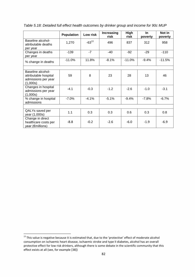
82
Table 5.18: Detailed full effect health outcomes by drinker group and income for 90c MUP
Population Low risk Increasing
risk High risk
In poverty
Not in poverty
Baseline alcohol-attributable deaths per year
1,270 -6313
496 837 312 958
Changes in deaths per year
-139 -7 -40 -92 -29 -110
% change in deaths -11.0% 11.8% -8.1% -11.0% -9.4% -11.5%
Baseline alcohol-attributable hospital admissions per year (1,000s)
59 8 23 28 13 46
Changes in hospital admissions per year (1,000s)
-4.1 -0.3 -1.2 -2.6 -1.0 -3.1
% change in hospital admissions
-7.0% -4.1% -5.1% -9.4% -7.8% -6.7%
QALYs saved per year (1,000s)
1.1 0.3 0.3 0.6 0.3 0.8
Change in direct healthcare costs per year (€millions)
-8.8 -0.2 -2.6 -6.0 -1.9 -6.9
13
This value is negative because it is estimated that, due to the ‘protective’ effect of moderate alcohol consumption on ischaemic heart disease, ischaemic stroke and type II diabetes, alcohol has an overall protective effect for low risk drinkers, although there is some debate in the scientific community that this effect exists at all (see, for example [38])

83
Table 5.19: Detailed breakdown of deaths and hospital admissions averted by health condition type for 90c MUP
Condition* Deaths per year (full
effect) Hospital admissions per year (full effect)
Alcoholic liver disease -41 -450
Cancers -29 -789
Alcoholic poisoning -12 -38
Alcoholic disorders (excl. liver disease) -12 -1031
Intentional self-harm -11 -35
Other diseases of the circulatory system -10 -351
Road traffic accidents -8 -173
Diseases of the digestive system -7 -79
Other accidents -6 -247
Hypertensive diseases -2 -621
Epilepsy and status epilepticus -1 -79
Assault -1 -54
Diabetes mellitus 0 -20
Other alcohol-related conditions 0 -136
*Alcoholic liver disease – K70, Cancers – C00-14, C15, C18, C20, C22, C32, C50; Alcoholic poisoning – T51, X45, Y15, R78.0; Alcoholic disorders (excl. liver
disease) – E24.4, G31.2, G62.1, G72.1, I42.6, K29.2, K86.0, F10; Intentional self-harm – X60-84; Other diseases of the circulatory system – I20-25, I47-48, I60-62, I69.0-69.2, I66, I69.3, I69.4; Road traffic accidents - V12-14, V19.4-19.6, V19.9, V20-28, V29-79, V80.3-80.5, V81.1, V82.1, V83-86, V87.0-87.9, V89.2, V89.3, V89.9; Diseases of the digestive system – I85, K22.6, K73, K74, K80, K85, K86.1; Other accidents – V02-04, V06.1, V09.2, V09.3, V90-94, V95-97, W00-19, W24-31, W32-34, W65-74, W78, X00-09, X31; Hypertensive diseases – I10-15; Epilepsy and status epilepticus – G40-41; Assault – X85-Y09; Diabetes Mellitus – E11; Other alcohol-related conditions – L40 excl. L40.5, O03.
Table 5.20: Effects of 90c MUP on death and hospital admissions by drinker group
Annual reductions following policy implementation
Low risk Increasing risk High risk Total
Deaths Admissions Deaths Admissions Deaths Admissions Deaths Admissions
Year 1 -9 -314 -18 -518 -26 -749 -52 -1582
Year 5 -8 -335 -25 -765 -49 -1518 -83 -2618
Year 10 -8 -340 -30 -922 -63 -1962 -101 -3224
Year 15 -8 -336 -36 -1064 -79 -2311 -122 -3711
Year 20 -7 -327 -40 -1183 -92 -2592 -139 -4102
Table 5.21: Effects of 90c MUP on deaths and hospital admissions by income group
Annual reductions following policy implementation
Poverty Not Poverty Total
Deaths Admissions Deaths Admissions Deaths Admissions
Year 1 -16 -540 -37 -1041 -52 -1582
Year 5 -20 -762 -63 -1856 -83 -2618
Year 10 -23 -886 -78 -2338 -101 -3224
Year 15 -26 -969 -96 -2742 -122 -3711
Year 20 -29 -1033 -110 -3070 -139 -4102

84
Figure 5.15: Effects of 90c MUP on deaths and hospital admissions by health condition
Alcoholic disorders (excl. liver disease) – E24.4, G31.2, G62.1, G72.1, I42.6, K29.2, K86.0, F10; Alcoholic liver disease – K70; Alcoholic poisoning – T51, X45, Y15, R78.0; Cancers – C00-14, C15, C18, C20, C22, C32, C50; Diabetes Mellitus – E11;
Epilepsy and status epilepticus – G40-41; Hypertensive diseases – I10-15; Other diseases of the circulatory system – I20-25, I47-48, I60-62, I69.0-69.2, I66, I69.3, I69.4; Diseases of the digestive system – I85, K22.6, K73, K74, K80, K85, K86.1; Road
traffic accidents - V12-14, V19.4-19.6, V19.9, V20-28, V29-79, V80.3-80.5, V81.1, V82.1, V83-86, V87.0-87.9, V89.2, V89.3, V89.9; Other accidents – V02-04, V06.1, V09.2, V09.3, V90-94, V95-97, W00-19, W24-31, W32-34, W65-74, W78, X00-09,
X31; Assault – X85-Y09; Intentional self-harm – X60-84; Other alcohol-related conditions – L40 excl. L40.5, O03

85
5.3 EXAMPLE POLICY ANALYSIS B: 100C MUP
This section describes the estimated impacts of a minimum unit price policy of 100c per standard
drink in detail. We assume that this threshold is updated annually in line with inflation. In addition to
the results already presented in Table 5.1 to Table 5.14, further detailed results are shown in Table
5.22 to Table 5.26 and in Figure 5.16 for consumption changes, consumer spending and health
outcomes including splitting effects into different types of alcoholic beverage.
Across the whole population, 37.5% of alcohol purchased would be affected (i.e. would have their
price raised to 100c). The proportion and absolute number of purchased standard drinks per week
affected for high risk drinkers (47.0% or 29.4 std. drinks) is substantially more than for increasing risk
drinkers (35.6% or 7.8 std. drinks) or low risk drinkers (33.4% or 1.1 std. drink). The proportion and
number of purchased standard drinks per week affected is slightly higher for those in poverty than
those above the poverty line (40.3% and 3.6 std. drinks vs. 36.9% and 3.5 std. drinks), though this
difference is primarily driven by a considerable difference between high risk drinkers in poverty
(57.5% or 43.3 std. drinks) vs. high risk drinkers not in poverty (44.0% or 26.2 std. drinks).
Across the whole population, mean weekly consumption is estimated to change by -8.8%.
Consumption is estimated to reduce by 0.83 std. drinks per person, or 1.06 std. drinks per drinker
per week. Weekly consumption reductions are greater for high risk drinkers (-15.1% or 9.47 std.
drinks) than low risk drinkers (-3.1% or 0.1 std. drinks) and for those in poverty (-12.3% or 1.6 std.
drinks) compared to those not in poverty (-8.1% or 1.0 std. drinks).
In both income groups, absolute reductions in consumption are estimated to be small for low risk
drinkers and much larger for high risk drinkers. However, for people below the poverty line the
relative change in consumption is similar across all drinkers, while for those above the poverty line
the relative changes are considerably larger for heavier drinkers. The estimated consumption
reduction for low risk drinkers in poverty is -12.0% or 0.5 std. drinks per week compared to -13.8% or
10.41 std. drinks per week for high risk drinkers in poverty. The corresponding figures for those not
in poverty are -1.4% or 0.01 std. drinks and -15.5% or 9.25 std. drinks.
Across the whole population, spending increases by 1.3% or €15.70 per drinker per year (€0.30 per
week). The cost impact of the policy on consumer spending varies significantly between different
drinker and income subgroups. Low risk and increasing risk drinkers are estimated to increase their
spending by €24.20 and €24.40 per year respectively, whilst high risk drinkers reduce their spending
by €106.60. Similar differences are observed between income subgroups, with those in poverty
saving €30.70 per year compared to a spending increase of €25.20 per year for those not in poverty.
Those in poverty are estimated to save money at all levels of consumption, with low risk,
increasing risk and high risk drinkers saving €6.80, €71.51 and €158.55 per year respectively. A
different pattern is observed for those not in poverty, with low risk and increasing risk drinkers
increasing their spending by €30.65 and €43.22 per year respectively, while high risk drinkers reduce
their spending by €94.14. These differing patterns are a result of both the different proportion of
each population subgroup’s purchases which are affected by the policy as well as the different price
elasticities of the beverages which make up a greater or lesser proportion of each subgroup’s
purchases.
86
Overall revenue to the Exchequer from duty and VAT receipts is estimated to reduce by 2.1% or
€34.3 million14.
Revenue to retailers is estimated to increase by €68.5million (18.1%) in the off-trade and
€9.3million (0.7%) in the on-trade. This is as reduced sales volumes are more than offset by the
increased value of remaining sales.
Effects on health are estimated to be substantial, with alcohol-attributable deaths estimated to
reduce by approximately 197 per year after 20 years, by which time the full effects of the policy will
be seen. Annual deaths are distributed differentially across drinker groups with approximately 12
saved amongst low risk drinkers, 57 amongst increasing risk drinkers and 128 amongst high risk
drinkers. Whilst those in poverty see a smaller absolute number of reduced deaths (42 vs. 155 for
those not in poverty), they also comprise a substantially smaller proportion of the population
(18.9%), meaning that the relative reduction in annual deaths per 100,000 population is greater
amongst those in poverty (6.2 vs. 5.4 per 100,000 for those not in poverty).
Similar patterns are observed amongst reductions in alcohol-related hospital admissions, with an
estimated 5,878 fewer admissions per year across the population. Admissions reductions for low
risk, increasing risk and high risk drinkers are 550, 1,700 and 3,620 respectively. Again, those in
poverty experience a lower absolute reduction in hospital admissions (1,520 vs. 4,350) but a larger
reduction per 100,000 population (227 vs. 151). Direct healthcare costs are estimated to reduce by
€7.4m in year 1 and €254.7m cumulatively over the first 20 years of the policy.
Crime is estimated to fall by 1,493 offences per year overall. Reductions are spread relatively
evenly between drinker groups, with 461, 547 and 485 fewer offences committed by low risk,
increasing risk and high risk drinkers respectively. However, it should be noted that increasing risk
and high risk drinkers (16% and 5% respectively) make up a considerably smaller proportion of the
population than low risk drinkers (78%). Costs of crime and policing are estimated to reduce by
€7.0m in year 1 and by €102.7 cumulatively over 20 years.
Workplace absence is estimated to be reduced by 115,600 per year. This is estimated to lead to an
annual saving of €16.1m in year 1 and €236.6m over 20 years.
The total societal value of these reductions in health, crime and workplace harms is estimated at
€1.7bn over the 20 year period modelled. This includes direct healthcare costs (€255m), crime costs
(€103m), workplace costs (€237m) and a financial valuation of the QALY gain (€1.1bn), assuming a
QALY is valued at €45,000. All costs and benefits are discounted at 3.5%.
14
Please also see note in Section 6.4 on VAT reclaims

87
Table 5.22: Detailed consumption and spending results for 100c MUP
Population Male Female In
poverty Not in
poverty Low risk Increasing
risk High risk
Baseline statistics
Baseline Consumption (std. drinks per week)
9.4 12.8 6.0 8.9 9.5 3.2 21.9 62.5
Population size 3,551,435 1,762,4
37 1,788,99
8 670,889
2,880,546
2,784,491 582,424 184,520
Baseline Consumption (drinker)
12.0 16.1 7.9 12.7 11.9 4.5 21.9 62.5
Drinker population 2,766,183 1,401,5
41 1,364,64
2 471,295
2,294,888
1,999,240 582,424 184,520
% drinkers 77.9% 79.5% 76.3% 70.2% 79.7% 71.8% 100.0% 100.0%
Sales/Consumption volume, std. drinks per drinker per year Off-beer 108.7 173.6 42.0 160.7 98.0 29.9 172.8 760.3 Off-cider 28.7 32.4 25.0 51.6 24.0 9.1 31.5 232.6 Off-wine 109.3 94.9 124.0 67.5 117.9 43.8 220.2 468.3 Off-spirits 40.4 44.3 36.5 36.9 41.1 15.5 58.5 254.1 Off-RTDs 1.8 0.9 2.8 4.5 1.3 1.3 3.8 1.4 On-beer 230.2 393.8 62.1 212.8 233.8 82.1 462.6 1100.8 On-cider 32.6 40.6 24.4 43.4 30.4 11.4 43.4 228.0 On-wine 24.3 14.9 34.0 15.2 26.2 17.4 44.2 36.5 On-spirits 49.6 43.8 55.6 65.1 46.5 23.8 98.8 174.6 On-RTDs 2.3 0.2 4.4 5.5 1.6 1.5 4.4 3.9 Total 628.0 839.5 410.8 663.2 620.7 235.8 1140.2 3260.5
Spending, euros per drinker per year
Off-beer 93.6 150.5 35.1 147.3 82.6 27.3 162.3 594.8 Off-cider 21.2 25.2 17.1 26.8 20.0 8.4 22.9 153.9 Off-wine 118.0 93.0 143.7 79.0 126.0 56.7 236.1 409.9 Off-spirits 47.5 62.6 32.0 24.0 52.3 11.4 47.4 439.1 Off-RTDs 1.0 0.6 1.5 1.8 0.9 1.5 0.0 0.0 On-beer 515.8 860.4 161.9 461.6 527.0 194.3 1074.4 2236.0 On-cider 72.6 86.2 58.6 81.5 70.8 25.4 100.9 494.3 On-wine 78.1 46.8 110.3 33.7 87.2 58.3 141.3 93.2 On-spirits 222.2 193.2 251.9 232.1 220.1 117.8 429.4 698.9 On-RTDs 5.4 0.0 10.9 7.6 4.9 6.5 3.1 0.0
Total 1175.3 1518.6 822.8 1095.3 1191.8 507.6 2217.7 5120.0
After intervention / Change from baseline Changes in consumption (std. drinks per drinker)
-1.1 -1.7 -0.4 -1.6 -1.0 -0.1 -1.6 -9.5
Changes in consumption (%)
-8.8% -10.7% -4.9% -12.3% -8.1% -3.1% -7.2% -15.1%
Final Consumption (drinker)
11.0 14.4 7.5 11.2 10.9 4.4 20.3 53.1
Absolute change in sales/Consumption volume, std. drinks per drinker per year Off-beer -43.3 -72.5 -13.3 -56.8 -40.5 -9.0 -61.3 -358.1 Off-cider -9.0 -13.1 -4.8 -8.0 -9.2 -2.4 -15.1 -61.2
Off-wine 1.1 3.3 -1.1 -4.0 2.2 1.8 4.8 -18.1
Off-spirits -4.6 -7.1 -2.1 -2.9 -5.0 -1.7 -7.7 -27.4 Off-RTDs -0.7 -0.4 -1.1 -1.6 -0.5 -0.4 -1.9 -0.6 On-beer -4.1 -6.0 -2.2 -8.0 -3.4 0.6 -7.0 -46.5 On-cider 3.2 4.6 1.8 0.0 3.9 1.8 3.3 18.9 On-wine 2.7 2.0 3.5 0.8 3.1 1.8 5.3 4.9 On-spirits -1.2 -0.7 -1.7 -2.2 -1.0 0.0 -3.3 -6.7 On-RTDs 0.5 0.1 1.0 1.2 0.4 0.3 1.1 0.8 Total -55.4 -89.9 -20.0 -81.7 -50.0 -7.3 -81.8 -493.9
Absolute change in spending, euros per drinker per year Off-beer -12.4 -21.5 -3.2 -19.0 -11.1 -1.6 -15.0 -121.9 Off-cider -3.0 -4.7 -1.3 -0.7 -3.5 -1.0 -6.7 -13.7 Off-wine 24.0 22.0 26.0 9.9 26.9 10.2 46.8 101.1 Off-spirits 2.4 -1.5 6.4 2.8 2.3 2.5 4.6 -5.6 Off-RTDs -0.3 -0.3 -0.4 -0.8 -0.2 -0.4 0.0 0.0 On-beer -8.3 -11.3 -5.3 -18.2 -6.3 2.5 -16.6 -99.2 On-cider 7.4 10.6 4.1 -0.4 9.0 4.2 7.2 43.4 On-wine 8.9 6.1 11.9 1.0 10.6 5.8 18.2 13.7 On-spirits -4.2 -2.0 -6.4 -6.7 -3.7 0.5 -13.9 -24.4 On-RTDs 1.2 0.0 2.5 1.4 1.2 1.4 0.8 0.0 Total 15.7 -2.5 34.5 -30.7 25.2 24.2 25.4 -106.6

88
Table 5.23: Detailed income and drinker group-specific results for 100c MUP
In Poverty Not in Poverty
Low risk Increasing risk High risk Low risk Increasing risk High risk
Baseline statistics Baseline Consumption (std. drinks per week) 2.6 21.1 75.3 3.4 22.0 59.5
Population size 544,638 90,629 35,623 2,239,854 491,795 148,897 Baseline Consumption (drinker) 4.1 21.1 75.3 4.6 22.0 59.5
Drinker population 345,044 90,629 35,623 1,654,196 491,795 148,897 % drinkers 63.4% 100.0% 100.0% 73.9% 100.0% 100.0%
Sales/Consumption volume, std. drinks per drinker per year Off-beer 31.6 174.4 1376.5 29.5 172.4 612.9 Off-cider 13.9 24.4 486.1 8.1 32.8 171.9 Off-wine 27.1 112.6 343.7 47.3 240.1 498.1 Off-spirits 19.1 45.5 188.6 14.7 60.8 269.7 Off-RTDs 3.8 7.6 2.7 0.8 3.1 1.1 On-beer 73.6 433.8 998.2 83.9 467.8 1125.4 On-cider 12.1 75.0 266.5 11.3 37.6 218.8 On-wine 9.5 37.8 13.1 19.0 45.4 42.1 On-spirits 18.7 172.0 242.5 24.8 85.3 158.4 On-RTDs 2.6 15.9 7.4 1.3 2.3 3.0 Total 211.9 1099.2 3925.3 240.7 1147.7 3101.4
Spending, euros per drinker per year
Off-beer 29.3 120.4 1358.8 26.9 170.1 412.0 Off-cider 9.3 9.6 239.6 8.2 25.4 133.4 Off-wine 71.0 78.1 157.9 53.7 265.2 470.2 Off-spirits 11.9 16.2 162.0 11.3 53.2 505.4 Off-RTDs 2.5 0.0 0.0 1.2 0.0 0.0 On-beer 170.7 972.4 1979.2 199.3 1093.2 2297.5 On-cider 14.4 176.2 490.1 27.7 87.0 495.2 On-wine 32.9 49.7 0.0 63.6 158.1 115.5 On-spirits 76.7 652.6 667.5 126.4 388.2 706.4 On-RTDs 10.3 0.0 0.0 5.7 3.6 0.0 Total 429.1 2075.2 5055.0 524.0 2244.0 5135.5
After intervention / Change from baseline
Changes in consumption (std. drinks per drinker)
-0.5 -2.2 -10.4 -0.1 -1.5 -9.2
Changes in consumption (%) -12.0% -10.4% -13.8% -1.4% -6.6% -15.5% Final Consumption (drinker) 3.6 18.9 64.9 4.6 20.6 50.2
Absolute change in sales/Consumption volume, std. drinks per drinker per year
Off-beer -12.7 -74.1 -440.4 -8.3 -58.9 -338.4 Off-cider -5.9 -13.2 -15.4 -1.7 -15.5 -72.2 Off-wine -0.6 -6.4 -30.7 2.3 6.9 -15.1 Off-spirits -2.2 -4.2 -6.5 -1.5 -8.3 -32.4 Off-RTDs -1.2 -3.7 -0.6 -0.2 -1.5 -0.6 On-beer -4.0 -7.5 -47.3 1.6 -6.9 -46.3 On-cider 0.5 -3.2 2.6 2.0 4.5 22.8 On-wine 0.5 1.9 0.4 2.0 5.9 6.0 On-spirits -0.3 -8.2 -5.8 0.0 -2.4 -6.9 On-RTDs 0.4 4.1 1.0 0.3 0.6 0.8 Total -25.4 -114.6 -542.8 -3.5 -75.7 -482.2
Absolute change in spending, euros per drinker per year Off-beer -3.7 -22.8 -157.1 -1.1 -13.6 -113.5
Off-cider -3.0 -7.3 37.6 -0.5 -6.6 -26.0 Off-wine 6.3 12.2 38.7 11.1 53.1 116.1 Off-spirits 1.1 2.0 21.2 2.8 5.1 -12.0 Off-RTDs -1.1 0.0 0.0 -0.3 0.0 0.0 On-beer -9.3 -20.2 -98.7 5.0 -15.9 -99.3 On-cider 0.6 -9.2 11.9 4.9 10.2 50.9 On-wine 1.2 0.4 0.0 6.7 21.5 17.0 On-spirits -0.9 -26.6 -12.3 0.8 -11.5 -27.3 On-RTDs 1.9 0.0 0.0 1.3 1.0 0.0 Total -6.8 -71.5 -158.5 30.7 43.2 -94.1

89
Table 5.24: Relative changes in price, consumption and spending, by beverage type and location for 100c MUP
Change in price
Change in consumption
Change in spending
Off-trade beer 44.2% -39.9% -13.3%
Off-trade cider 24.9% -31.4% -14.2%
Off-trade wine 19.1% 1.0% 20.3%
Off-trade spirits 18.6% -11.5% 5.0%
Off-trade RTDs 15.9% -40.0% -30.5%
Subtotal: Off-trade 29.0% -19.6% 3.8%
On-trade beer 0.2% -1.8% -1.6%
On-trade cider 0.3% 9.9% 10.2%
On-trade wine 0.2% 11.2% 11.4%
On-trade spirits 0.5% -2.4% -1.9%
On-trade RTDs -0.4% 23.1% 22.7%
Subtotal: On-trade 0.2% 0.3% 0.6%
Subtotal: Beer
-14.0% -3.4%
Subtotal: Cider
-9.4% 4.7%
Subtotal: Wine
2.9% 16.8%
Subtotal: Spirits
-6.5% -0.7%
Subtotal: RTDs
-4.9% 13.9%
Total 11.1% -8.8% 1.3%
Table 5.25: Detailed full effect health outcomes by drinker group and income for 100c MUP
Population Low risk Increasing
risk High risk
In poverty
Not in poverty
Baseline alcohol-attributable deaths per year
1270 -63 496 837 312 958
Changes in deaths per year
-197 -12 -57 -128 -42 -155
% change in deaths -15.5% 18.8% -11.5% -15.3% -13.4% -16.2%
Baseline alcohol-attributable hospital admissions per year (1,000s)
59 8 23 28 13 46
Hospital admissions per year (1,000s)
-5.9 -0.55 -1.70 -3.62 -1.52 -4.35
% change in hospital admissions
-10.0% -6.9% -7.3% -13.2% -11.6% -9.5%
QALYs saved per year (1,000s)
1.6 0.4 0.4 0.8 0.4 1.2
Healthcare costs per year (€millions)
-12.6 -0.4 -3.7 -8.5 -2.9 -9.7

90
Table 5.26: Detailed breakdown of deaths and hospital admissions averted by health condition type for 100c MUP
Condition* Deaths per year (full
effect) Hospital admissions per year (full effect)
Alcoholic liver disease -57 -621
Cancers -41 -1123
Alcoholic poisoning -17 -55
Alcoholic disorders (excl. liver disease) -17 -1485
Intentional self-harm -15 -50
Other disease of the circulatory system -14 -482
Road traffic accidents -12 -246
Diseases of the digestive system -10 -110
Other accidents -8 -358
Hypertensive diseases -3 -930
Epilepsy and status epilepticus -2 -114
Assault -1 -77
Diabetes mellitus 0 -25
Other alcohol-related conditions 0 -202
*Alcoholic liver disease – K70, Cancers – C00-14, C15, C18, C20, C22, C32, C50, Alcoholic poisoning – T51, X45, Y15, R78.0, Alcoholic disorders (excl. liver
disease) – E24.4, G31.2, G62.1, G72.1, I42.6, K29.2, K86.0, F10, Intentional self-harm – X60-84, Other diseases of the circulatory system – I20-25, I47-48, I60-62, I69.0-69.2, I66, I69.3, I69.4, Road traffic accidents - V12-14, V19.4-19.6, V19.9, V20-28, V29-79, V80.3-80.5, V81.1, V82.1, V83-86, V87.0-87.9, V89.2, V89.3, V89.9, Diseases of the digestive system – I85, K22.6, K73, K74, K80, K85, K86.1, Other accidents – V02-04, V06.1, V09.2, V09.3, V90-94, V95-97, W00-19, W24-31, W32-34, W65-74, W78, X00-09, X31, Hypertensive diseases – I10-15, Epilepsy and status epilepticus – G40-41, Assault – X85-Y09, Diabetes Mellitus – E11, Other alcohol-related conditions – L40 excl. L40.5, O03.
Table 5.27: Effects of 100c MUP on death and hospital admissions by drinker group
Annual reductions following policy implementation
Low risk Increasing risk High risk Total
Deaths Admissions Deaths Admissions Deaths Admissions Deaths Admissions
Year 1 -13 -492 -25 -741 -37 -1062 -75 -2295
Year 5 -12 -534 -36 -1100 -70 -2144 -118 -3778
Year 10 -12 -549 -42 -1325 -89 -2761 -143 -4636
Year 15 -12 -556 -50 -1530 -111 -3239 -173 -5325
Year 20 -12 -553 -57 -1702 -128 -3623 -197 -5878
Table 5.28: Effects of 100c MUP on deaths and hospital admissions by income group
Annual reductions following policy implementation
Poverty Not Poverty Total
Deaths Admissions Deaths Admissions Deaths Admissions
Year 1 -22 -773 -53 -1522 -75 -2295
Year 5 -29 -1118 -89 -2661 -118 -3778
Year 10 -33 -1309 -110 -3326 -143 -4636
Year 15 -38 -1431 -135 -3894 -173 -5325
Year 20 -42 -1524 -155 -4354 -197 -5878

91
Figure 5.16: Effects of 100c MUP on deaths and hospital admissions
Alcoholic disorders (excl. liver disease) – E24.4, G31.2, G62.1, G72.1, I42.6, K29.2, K86.0, F10; Alcoholic liver disease – K70; Alcoholic poisoning – T51, X45, Y15, R78.0; Cancers – C00-14, C15, C18, C20, C22, C32, C50; Diabetes Mellitus – E11;
Epilepsy and status epilepticus – G40-41; Hypertensive diseases – I10-15; Other diseases of the circulatory system – I20-25, I47-48, I60-62, I69.0-69.2, I66, I69.3, I69.4; Diseases of the digestive system – I85, K22.6, K73, K74, K80, K85, K86.1; Road
traffic accidents - V12-14, V19.4-19.6, V19.9, V20-28, V29-79, V80.3-80.5, V81.1, V82.1, V83-86, V87.0-87.9, V89.2, V89.3, V89.9; Other accidents – V02-04, V06.1, V09.2, V09.3, V90-94, V95-97, W00-19, W24-31, W32-34, W65-74, W78, X00-09,
X31; Assault – X85-Y09; Intentional self-harm – X60-84; Other alcohol-related conditions – L40 excl. L40.5, O03

92
5.4 SENSITIVITY ANALYSES
Table 5.29, Figure 5.17 and Figure 5.18 compare the estimated impacts on alcohol consumption of a
90c MUP and a ban on off-trade promotions using alternative elasticity estimates as described in
Section 4.7.
Table 5.29: Comparison of estimated impacts on alcohol consumption for a 90c MUP and off-trade promotion ban using alternative elasticity estimates
90c MUP: alternative elasticities
Base case SA1:
NADS elasticities
SA2: No cross-
price
SA3: No non-
significant
SA4: Consumption level-
specific
Population -6.2% -27.6% -7.6% -7.1% -5.6%
Low risk -1.9% -23.4% -4.6% -4.3% -4.8%
Increasing risk
-5.1% -25.9% -6.0% -5.8% -4.7%
High risk -10.7% -32.7% -11.8% -10.6% -7.1%
In poverty -8.7% -18.4% -8.6% -7.5% -3.9%
Not in poverty
-5.6% -29.6% -7.4% -7.0% -5.9%
Ban on off-trade promotions: alternative elasticities
Base case SA1:
NADS elasticities
SA2: No cross-
price
SA3: No non-
significant
SA4: Consumption level-
specific
Population -1.8% -9.6% -2.2% -2.0% -1.5%
Low risk -0.7% -8.6% -1.4% -1.2% -1.8%
Increasing risk
-1.4% -9.8% -1.8% -1.7% -1.2%
High risk -3.0% -10.1% -3.2% -2.8% -1.5%
In poverty -2.6% -6.8% -2.3% -2.0% -1.2%
Not in poverty
-1.6% -10.2% -2.2% -1.9% -1.5%

93
Figure 5.17: Comparison of estimated impacts on alcohol consumption of a 90c MUP policy using alternative elasticity estimates
Figure 5.18: Comparison of estimated impacts on alcohol consumption of an off-trade promotion ban using alternative elasticity estimates
The results for a 90c MUP suggest that the base case model is relatively conservative in terms of
estimated scale of impact for the overall population when compared to the alternative sensitivity
analyses. Only SA4 estimates a slightly lower estimated reduction in population consumption of -
5.6% compared to -6.2% for the base case. The impacts estimated using the NADS-derived
elasticities (SA1) are substantially larger than any of the other alternatives considered and may be
considered to be implausible. The effects of the different sensitivity analyses are not uniform across
-35%
-30%
-25%
-20%
-15%
-10%
-5%
0%
Population Low risk Hazardous Harmful In povertyNot in
poverty
% r
ed
uct
ion
in c
on
sum
pti
on
fo
r 9
0c
MU
P
Base case
SA1
SA2
SA3
SA4
-12%
-10%
-8%
-6%
-4%
-2%
0%
Population Low risk Hazardous Harmful In povertyNot in
poverty
% r
ed
uct
ion
in c
on
sum
pti
on
fo
r p
rom
oti
on
b
an
Base case
SA1
SA2
SA3
SA4

94
subgroups, for example SA4 shows a smaller impact on those in poverty, while SA2 shows a greater
impact on high risk drinkers. Results for an off-trade promotion ban are very similar, though the
absolute magnitude of the estimated consumption reductions in smaller.

95
6 DISCUSSION
This research study presents the synthesis of evidence available to undertake policy appraisal of 21
options for price regulation of alcohol in Ireland. In this discussion section, we draw out the key
themes and findings from the detailed analysis.
6.1 DIFFERENTIAL POLICY IMPACTS
We have examined 9 policy options for a minimum price threshold ranging from 40c to 120c per
standard drink. The estimated per person reduction in alcohol consumption for the overall
population ranges from 0.0% to 14.6% for an MUP policy within this range, with higher MUP
thresholds leading to greater reductions in consumption. These consumption reductions lead to
estimated reductions in deaths from 1 to 312 per year, hospital admissions from 46 to 9,483 per
year, crime from 2 to 2,453 per year and days absence from work from 500 to 197,100 per year,
again with higher MUP thresholds leading to greater reductions in alcohol-related harms.
Specifically, a 90c MUP policy is estimated to reduce per person alcohol consumption by 6.2% and
lead to 139 fewer deaths, 4,102 fewer hospital admissions, 1,043 fewer crimes and 77,800 fewer
absent days in Ireland per year.
In contrast, a policy to ban below-cost selling has virtually no impact on consumption and alcohol-
related harms because most alcohol sold in the market would not be affected by the policy.
A policy to ban all price-based promotion in the off-trade is estimated to reduce per person alcohol
consumption by 1.8% and leads to 45 fewer deaths, 1,382 fewer hospital admissions, 271 fewer
crimes and 21,400 fewer absent days in Ireland per year. The same pattern of consumption and
harm reductions is found for policies combining MUP and a ban on price-based promotion in the off-
trade, with higher MUP thresholds leading to greater reductions in consumption and alcohol-related
harms. For the same MUP threshold, a combined policy is more effective in consumption and harm
reduction than the single MUP policy, but the additional benefit is diminishing as the MUP threshold
increases. For example, per person consumption reductions for without a promotions ban versus
with the promotions ban are estimated to be 0.7% versus 2.6% (difference is 1.9%) for a 60c MUP,
6.2% versus 7.1% (difference is 0.9%) for 60c, and there is no difference for a 120c MUP.
In summary, MUP policies are estimated to reduce alcohol consumption and alcohol-related
mortality, hospital admissions, crime and absence from work in Ireland either as a single policy or in
combination with a ban on price-based promotion in the off-trade; and the higher the threshold at
which an MUP is set, the greater the reduction in alcohol consumption and alcohol-related harms.

96
6.2 IMPACTS BY DRINKER GROUP
In line with findings from previous studies in England, Scotland and Canada, this analysis shows that
MUP is a policy targeted at increasing risk and high risk drinkers [2], [3], [6]. The main reason for this
is that high risk drinkers tend to favour the cheaper alcohol, which is the alcohol most affected by
MUP policies. See for example Figure 4.8 which shows that high risk drinkers buy almost half of their
alcohol at below 90c per standard drink, whereas low risk drinkers buy around a third of their
alcohol below this threshold.
A 90c MUP is estimated to reduce alcohol consumption by 1.9%, 5.1% and 10.7% for low risk,
increasing risk and high risk drinkers respectively. The absolute reduction in standard drinks
consumed is estimated at 0.1 per week for low risk drinkers, 1.1 per week for increasing risk, and 6.7
per week for high risk drinkers. So it is the high risk drinkers who are most affected in terms of scale
of consumption reduction.
This in turn is reflected in the harm reductions for the 90c MUP policy. High risk drinkers, who make
up 5% of the population, benefit from 92 out of 139 (66%) and 2,600 out of 4,100 (63%) estimated
annual reductions in deaths and hospital admissions from the policy.
6.3 IMPACTS BY INCOME
The analyses also present income-specific results from SAPM3 for Ireland and five main findings
should be highlighted.
First, when interpreting these results, it should be borne in mind that 29.8% of those in poverty are
non-drinkers compared to 20.3% of those not in poverty and, amongst low risk drinkers, those in
poverty consume 4.1 standard drinks per week compared to 4.6 standard drinks for those not in
poverty. Therefore, the subgroup of the population which is in poverty contains a disproportionate
number of people who will be wholly or largely unaffected by the direct impacts of MUP due to their
abstinence or relatively low consumption.
Second, MUP impacts on the consumption of both in poverty and not in poverty income groups;
however, it has a greater relative impact on the consumption of drinkers in poverty. As we assume
drinkers in poverty and not in poverty are equally responsive to price changes when they have the
same consumption patterns, this difference in estimated policy impact is due to 1) drinkers in
poverty tending to buy more products from the cheaper end of the spectrum, and 2) the larger price
elasticities of the products favoured by drinkers in poverty, particularly beer and cider purchased in
the off-trade.
Third, the impact of a 90c MUP on some groups is very small in absolute terms. Consumption
amongst low risk drinkers in poverty and not in poverty respectively would fall by just 18.1 and 1.5
standard drinks per year. This compares with an average reduction of 383 standard drinks for in
poverty high risk drinkers and 342 standard drinks for not in poverty high risk drinkers.
Fourth, the impact of a MUP on the spending of drinkers in poverty is smaller overall than the
impact on spending of drinkers who are not in poverty. This is because the products favoured by
drinkers not in poverty have smaller price elasticities and thus, although drinkers not in poverty do

97
reduce their consumption, they are also more likely to increase their spending in response to price
increases.
Finally, the greater fall in consumption amongst drinkers in poverty also leads to greater reductions
in alcohol-related health harms within this group considering that they make up only 19% of the
population. For a 90c MUP, the estimated reductions in deaths are 4.4 and 3.8 per 100,000
population for drinkers in poverty and not in poverty respectively. For hospital admissions, the
estimated reductions are 153.9 and 106.6 per 100,000 population for drinkers in poverty and not in
poverty.
In summary, the income-specific analysis of the potential impacts of a 90c MUP suggests that MUP
will impact on both drinkers in poverty and not in poverty and that, within each income group, the
impacts on high risk drinkers will be substantial and greater than the impacts on low risk drinkers. A
key policy concern is whether low risk drinkers in poverty are ‘penalised’ by MUP. Policy impacts on
low risk drinkers in poverty are small in absolute terms, amounting to a consumption reduction of
just 18.1 standard drinks per year and a spending reduction of €4.50 per year. As low risk consumers
make up 95.4% of the in poverty population and 36.6% of these are abstainers and thus not directly
affected by the policy, our estimates suggest only a small minority of those in poverty will be
substantially impacted by MUP and these individuals will be those who, though in poverty, consume
at increasing risk or high risk levels. The greater health benefits of MUP for drinkers in poverty
suggest the policy may also contribute to the reduction of health inequalities.
6.4 IMPACTS ON REVENUE TO THE EXCHEQUER AND RETAILERS
When prices and consumption change then the revenue to government will change also because
duty is levied on amount of ethanol content (e.g. beer and spirits) or product volume (e.g. wine and
cider) that is sold, and VAT is charged on the sales value.
A 90c MUP is estimated to lead to an overall decrease in revenue for the Exchequer of €21.4 m
(1.3%), with a decrease in duty plus VAT revenue from the off-trade of €26.1m (6.5%) and a small
increase from the on-trade of €4.8m (0.4%). The decrease in duty plus VAT revenue from the off-
trade is mainly due to the decrease in off-trade duty receipts which are directly linked to the
reduction in alcohol consumption, as duty is levied on either ethanol content (e.g. beer and spirits)
or product volume (e.g. wine and cider). It is important to note that these estimates do not account
for current VAT reclaims on products sold below the cost of production. MUP policies are likely to
significantly reduce the amount of alcohol sold at below cost and, as a consequence, the associated
VAT reclaims. Unofficial estimates place the annual reclaim at €21million [34], suggesting the actual
impact on revenue to the Exchequer of the modelled policies may be somewhat smaller than the
estimates presented here.
Retailers’ revenues are affected to a larger extent than those of government. A 90c MUP is
estimated to lead to an overall increase in revenue for retailers of €62.6m (3.8%), with increase in
revenue for off-trade retailers of €53.3m (14.1%) and for on-trade retailers of €9.3m (0.7%).
The relative inelasticity of alcohol (see Table 4.3 where most estimated own-price elasticities are
smaller than 1) means that the average consumer response to alcohol price increases includes

98
paying more as well as buying less, and when elasticities are less than 1, spending and hence
revenue to retailers increases even though consumption falls.
Table 4.3 also shows that there is a mix of positive and negative cross-price elasticities of demand for
on-trade beverages with regard to off-trade prices, and the magnitude of these cross-price
elasticities are smaller than the own-price elasticities. This leads to the small increase in revenue for
on-trade retailers even though the prices of products in the on-trade are largely unaffected by the
policy.
Caution is required regarding the estimated impacts on revenue for on-trade due to the lack of
statistical significance for many of the cross-price elasticities.
It should also be noted that considerable uncertainty exists regarding retailers’ responses to the
introduction of a MUP. SAPM3 assumes the only change in pricing that will occur is for all prices of
products below the MUP threshold to be raised up to that threshold. In reality, retailers and
producers may make a range of additional changes to both prices and products which may impact
on resulting revenue changes to the Exchequer and retailers and other modelled outcomes.
6.5 IMPACTS ON ALCOHOL-RELATED HEALTH
A 90c MUP policy is estimated to lead to 139 fewer deaths and 4102 fewer hospital admissions per
year at full effect. As illustrated in Tables 5.9 and 5.10, the impact on acute health conditions is felt
immediately, whilst the reduction in deaths and admissions from chronic causes increases steadily
across the first 20 years of the policy. Tables 5.20 and 5.21 show that the impact on health across
time varies by drinker and income group, for example, whilst the majority of health gains for low risk
drinkers are experienced in the short term, the full benefits for high risk drinkers take longer to
develop, with the full effect only being felt after 20 years. The savings to the Health Service from
these reductions in alcohol-related illness are estimated to be €5.2million in the first year following
implementation of the policy, with higher MUP thresholds providing even greater benefits.
These figures are likely to underestimate the true impact as the morbidity data is based on hospital
in-patient admissions data and therefore excludes patients presenting at either Accident and
Emergency (A&E) departments or in primary care who do not subsequently go on to attend hospital
for the same condition. This is particularly likely to lead to an underestimate of the true prevalence
of some acute health conditions such as ethanol poisoning or falls where patients are more likely to
be treated at A&E and then sent home directly. It is also likely that the cost savings to the Health
Service are underestimated as they do not include any A&E or primary care related costs, both of
which are likely to reduce to some extent following the introduction of any of the modelled policies.
Finally, it should be noted that the existing evidence on the temporal relationship between changes
in alcohol consumption and changes in risk is relatively limited. For those chronic health conditions
for which no evidence could be identified we have assumed that the change in risk is linear over 20
years. This is likely to be conservative as the available evidence for other conditions suggests that
the greatest reduction in risk occurs in the years immediately after the change in consumption [28].
In terms of the partial effects analysis presented in Table 5.9, Table 5.10 , Table 5.20, Table 5.21,

99
Figure 5.11 and Figure 5.12 this suggests that the actual impact of the modelled policies on deaths
and hospital admissions at years 1 and 5 in particular may be underestimated.
6.6 IMPACTS ON ALCOHOL-RELATED CRIME
A 90c MUP is estimated to lead to 1,043 fewer crimes. High risk drinkers, who comprise around 5%
of the population, account for 33% of this reduction. Costs of crime are estimated to reduce by
€4.9m in year 1 under this policy, with higher MUP thresholds providing even greater savings (e.g.
€11.5m in year 1 for a 120c MUP). Unlike health gains, which increase over time, the full impact of
an MUP policy on crime would be experienced within the first year.
This is most likely to be an underestimation of the true impact because 1) The AAF estimates used to
calibrate the crime risk functions (see Section 4.5.3) which were derived from the Offending Crime
and Justice Survey were based on a question asking respondents whether alcohol was one of the
reasons for committing the crime, rather than a question asking whether the offender was drunk
when the crime was committed. It is likely that the responses to the former question underestimate
the impact of alcohol on crime levels, whilst the latter question would overestimate this impact; and
2) the crime categories shown in Table 4.8 and included in the model exclude a number of offences
which have some alcohol-related component (e.g. drink-driving and public disorder offences). These
offences were excluded because of either a lack of evidence on the AAF of the offence or because of
a lack of available evidence on the valuation of the harm.
6.7 IMPACTS ON WORK ABSENCE
Workplace absence is estimated to fall under all modelled policies, with a reduction of 77,800 days
absent per year for a 90c MUP, valued at €10.9m in the first year following implementation of the
policy. As with the impact on crime, the full impact of an MUP policy on work absence would be
experienced within the first year.
6.8 COST IMPACTS ON SOCIETY
A 90c MUP is estimated to lead to a cumulative saving to society of €1.2bn over 20 years from
reductions in direct health costs (€178m), crime costs (€72m), reduced workplace absence (€160m)
and gains in societal health (€775m). It should be noted that these figures do not include the
potential productivity gain to society of those people who live longer or in better health as a result
of the policy.
6.9 POTENTIAL IMPACT OF MUP AND PRICE-BASED PROMOTIONS BAN ON
CROSS-BORDER SHOPPING
Owing to the shared land border and differential tax regimes between the Republic of Ireland and
Northern Ireland, shopping trips across the border to Northern Ireland do occur. In 2010 the Irish
Quarterly National Household Survey (QNHS) included a series of questions on cross border
shopping in Northern Ireland by Irish residents [35]. The results of this survey show that in 2010 an
100
estimated 14% of households in Ireland made at least one shopping trip across the border, spending
an average of €274 per trip [35]. Of this total €33 (12%) was spent on alcohol on average, with the
majority (66%) being spent on groceries (€105) or clothing and other durables (€77). Households in
the Border region were more than twice as likely to have shopped across the border as those from
any other region (43% compared to 19% or less) and accounted for over half the total expenditure
on cross-border shopping (€240million out of €418million). Around three quarters (25.6%) of
spending cross-border was on dedicated shopping trips rather than expenditure on non-shopping
trips.
In addition to the QNHS figures, respondents to the NADS were asked whether the alcohol they had
purchased in the last week was purchased in the country or abroad (including Northern Ireland). An
exploratory analysis of this data suggests that survey respondents paid an average of 31% less per
standard drink for alcohol purchased abroad.
Taken together, these surveys suggest that Irish residents may be purchasing cheaper alcohol in
Northern Ireland. However; the fact that alcohol represents a relatively small percentage of the total
spend on cross-border shopping trips suggests that it may not be the principal motivation for most
of these trips. Whilst it is therefore likely that MUP policies or promotions bans which increase the
price of some alcohol may lead to some increase in cross-border purchasing in Northern Ireland,
reducing the estimated impact of the policies, it is probable that such changes in purchasing habits
will be small, especially for the large majority of the population (90%) who live outside the Border
region.
6.10 RELATIVE MERITS OF MUP AND PRICE-BASED PROMOTIONS BAN IN
COMPARISON WITH TAX INCREASES.
Modelling of taxation policies was out-with the scope of this report. It is nevertheless worthwhile
rehearsing for policy makers some key principles in terms of the difference in targeting between
MUP and general tax rises.
Firstly, MUP is targeted at increasing the price only of cheap alcohol sold below the MUP threshold.
In contrast, it is expected that a tax increase (most likely through increased duty rates) would
increase the price of all alcohol sold in the market because alcohol duties are levied on either
ethanol content or product volume. The likelihood is therefore that low risk drinkers would be much
more affected by a general tax rise than a MUP policy targeted at cheaper alcohol.
Secondly, there is the issue of whether and how retailers pass through the tax increases to
customers. A recent UK study shows that when duty increases, supermarkets have tended to
increase the price of more expensive alcohol more than the tax increase and increase the price of
cheaper alcohol less than the tax increase [36]. This in turn is likely to reduce the impact of the tax
policy on increasing and high risk drinkers and drinkers who prefer cheaper alcohol.

101
7 REFERENCES
[1] R. Purshouse, A. Brennan, N. Latimer, Y. Meng, R. Rafia, R. Jackson, and P. Meier, “Modelling to assess the effectiveness and cost-effectiveness of public health related strategies and interventions to reduce alcohol attributable harm in England using the Sheffield Alcohol Policy Model version 2.0,” Sheffield, 2009.
[2] Y. Meng, D. Hill-McManus, A. Brennan, and P. Meier, “Model-Based Appraisal of Alcohol Minimum Pricing and off-Licensed Trade Discount Bans in Scotland using the Sheffield Alcohol Policy Model (v.2): Second update based on newly available data,” Sheffield, 2012.
[3] D. Hill-McManus, A. Brennan, T. Stockwell, N. Giesbrecht, G. Thomas, J. Zhao, G. Martin, and A. Wettlaufer, “Model-Based Appraisal Of Alcohol Minimum Pricing In Ontario And British Columbia: A Canadian adaptation of the Sheffield Alcohol Policy Model Version 2,” 2012.
[4] C. Angus, E. Scafato, S. Ghirini, A. Torbica, F. Ferre, P. Struzzo, R. Purshouse, and A. Brennan, “Cost-effectiveness of a programme of screening and brief interventions for alcohol in primary care in Italy.,” BMC Fam. Pract., vol. 15, no. 1, p. 26, Jan. 2014.
[5] Y. Meng, A. Brennan, J. Holmes, D. Hill-McManus, C. Angus, R. Purshouse, and P. S. Meier, “Modelled income group-specific impacts of alcohol minimum unit pricing in England 2014/15: Policy appraisals using new developments to the Sheffield Alcohol Policy Model (v2.5),” 2013.
[6] J. Holmes, Y. Meng, P. S. Meier, A. Brennan, C. Angus, A. Campbell-Burton, Y. Guo, D. Hill-McManus, and R. C. Purshouse, “Effects of minimum unit pricing for alcohol on different income and socioeconomic groups: a modelling study.,” Lancet, vol. 383, no. 9929, pp. 1655–64, May 2014.
[7] P. S. Meier, Y. Meng, J. Holmes, B. Baumberg, R. Purshouse, D. Hill-McManus, and A. Brennan, “Adjusting for unrecorded consumption in survey and per capita sales data: quantification of impact on gender- and age-specific alcohol-attributable fractions for oral and pharyngeal cancers in Great Britain.,” Alcohol Alcohol, vol. 48, no. 2, pp. 241–9, Jan. 2013.
[8] J. Rehm, T. Kehoe, G. Gmel, F. Stinson, B. Grant, and G. Gmel, “Statistical modeling of volume of alcohol exposure for epidemiological studies of population health: the US example.,” Popul. Health Metr., vol. 8, no. 1, p. 3, Jan. 2010.
[9] T. Stockwell, J. Zhao, and S. Macdonald, “Who under-reports their alcohol consumption in telephone surveys and by how much? An application of the ‘yesterday method’ in a national Canadian substance use survey.,” Addiction, May 2014.
[10] A. Hope, “A standard drink in Ireland: What strength?,” 2009.
[11] Y. Meng, A. Brennan, R. Purshouse, D. Hill-McManus, C. Angus, J. Holmes, and P. S. Meier, “Estimation of own and cross price elasticities of alcohol demand in the UK-A pseudo-panel approach using the Living Costs and Food Survey 2001-2009.,” J. Health Econ., vol. 34, pp. 96–103, Mar. 2014.
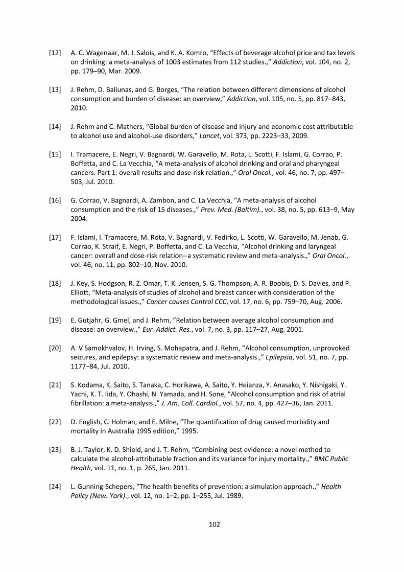
102
[12] A. C. Wagenaar, M. J. Salois, and K. A. Komro, “Effects of beverage alcohol price and tax levels on drinking: a meta-analysis of 1003 estimates from 112 studies.,” Addiction, vol. 104, no. 2, pp. 179–90, Mar. 2009.
[13] J. Rehm, D. Baliunas, and G. Borges, “The relation between different dimensions of alcohol consumption and burden of disease: an overview,” Addiction, vol. 105, no. 5, pp. 817–843, 2010.
[14] J. Rehm and C. Mathers, “Global burden of disease and injury and economic cost attributable to alcohol use and alcohol-use disorders,” Lancet, vol. 373, pp. 2223–33, 2009.
[15] I. Tramacere, E. Negri, V. Bagnardi, W. Garavello, M. Rota, L. Scotti, F. Islami, G. Corrao, P. Boffetta, and C. La Vecchia, “A meta-analysis of alcohol drinking and oral and pharyngeal cancers. Part 1: overall results and dose-risk relation.,” Oral Oncol., vol. 46, no. 7, pp. 497–503, Jul. 2010.
[16] G. Corrao, V. Bagnardi, A. Zambon, and C. La Vecchia, “A meta-analysis of alcohol consumption and the risk of 15 diseases.,” Prev. Med. (Baltim)., vol. 38, no. 5, pp. 613–9, May 2004.
[17] F. Islami, I. Tramacere, M. Rota, V. Bagnardi, V. Fedirko, L. Scotti, W. Garavello, M. Jenab, G. Corrao, K. Straif, E. Negri, P. Boffetta, and C. La Vecchia, “Alcohol drinking and laryngeal cancer: overall and dose-risk relation--a systematic review and meta-analysis.,” Oral Oncol., vol. 46, no. 11, pp. 802–10, Nov. 2010.
[18] J. Key, S. Hodgson, R. Z. Omar, T. K. Jensen, S. G. Thompson, A. R. Boobis, D. S. Davies, and P. Elliott, “Meta-analysis of studies of alcohol and breast cancer with consideration of the methodological issues.,” Cancer causes Control CCC, vol. 17, no. 6, pp. 759–70, Aug. 2006.
[19] E. Gutjahr, G. Gmel, and J. Rehm, “Relation between average alcohol consumption and disease: an overview.,” Eur. Addict. Res., vol. 7, no. 3, pp. 117–27, Aug. 2001.
[20] A. V Samokhvalov, H. Irving, S. Mohapatra, and J. Rehm, “Alcohol consumption, unprovoked seizures, and epilepsy: a systematic review and meta-analysis.,” Epilepsia, vol. 51, no. 7, pp. 1177–84, Jul. 2010.
[21] S. Kodama, K. Saito, S. Tanaka, C. Horikawa, A. Saito, Y. Heianza, Y. Anasako, Y. Nishigaki, Y. Yachi, K. T. Iida, Y. Ohashi, N. Yamada, and H. Sone, “Alcohol consumption and risk of atrial fibrillation: a meta-analysis.,” J. Am. Coll. Cardiol., vol. 57, no. 4, pp. 427–36, Jan. 2011.
[22] D. English, C. Holman, and E. Milne, “The quantification of drug caused morbidity and mortality in Australia 1995 edition,” 1995.
[23] B. J. Taylor, K. D. Shield, and J. T. Rehm, “Combining best evidence: a novel method to calculate the alcohol-attributable fraction and its variance for injury mortality.,” BMC Public Health, vol. 11, no. 1, p. 265, Jan. 2011.
[24] L. Gunning-Schepers, “The health benefits of prevention: a simulation approach.,” Health Policy (New. York)., vol. 12, no. 1–2, pp. 1–255, Jul. 1989.

103
[25] K. M. Fillmore, W. C. Kerr, T. Stockwell, T. Chikritzhs, and A. Bostrom, “Moderate alcohol use and reduced mortality risk: Systematic error in prospective studies,” Addict. Res. Theory, vol. 14, no. 2, pp. 101–132, Jan. 2006.
[26] HSE, “HSE.ie - Alcohol.” [Online]. Available: http://www.hse.ie/go/alcohol/.
[27] D. Hill-McManus, C. Angus, Y. Meng, J. Holmes, A. Brennan, and P. Sylvia Meier, “Estimation of usual occasion-based individual drinking patterns using diary survey data,” Drug Alcohol Depend., 2013.
[28] J. Holmes, P. S. Meier, A. Booth, Y. Guo, and A. Brennan, “The temporal relationship between per capita alcohol consumption and harm: a systematic review of time lag specifications in aggregate time series analyses.,” Drug Alcohol Depend., vol. 123, no. 1–3, pp. 7–14, Jun. 2012.
[29] L. Jones, M. Bellis, D. Dedman, H. Sumnall, and K. Tocque, “Alcohol-attributable fractions for England Alcohol-attributable mortality and hospital admissions,” North West Public Health Observatory, Centre for Public Health Research Directorate, Liverpool John Morres University, Liverpool, Liverpool, 2008.
[30] Cardiff Research Consortium, “Health Outcomes Data Repository,” 2011.
[31] Health Information and Quality Authority, “Guidelines for the Economic Evaluation of Health Technologies in Ireland,” 2010.
[32] “Revisions made to the multipliers and unit costs of crime used in the Integrated Offender Management Value for Money Toolkit.” [Online]. Available: https://www.gov.uk/government/uploads/system/uploads/attachment_data/file/118042/IOM-phase2-costs-multipliers.pdf. [Accessed: 27-May-2014].
[33] HM Treasury, “The green book: appraisal and evaluation in central government,” London: The Stationary Office, 2003.
[34] National Off-Licence Association, “National Off-Licence Association (NOffLA) Submission to the Minister for Finance for Budget 2014,” 2013.
[35] Central Statistics Office, “Quarterly National Household Survey: Household shopping, quarter 2 2010,” 2010.
[36] A. K. Ally, Y. Meng, R. Chakraborty, P. W. Dobson, J. S. Seaton, J. Holmes, C. Angus, Y. Guo, D. Hill-McManus, A. Brennan, and P. S. Meier, “Alcohol tax pass-through across the product and price range: do retailers treat cheap alcohol differently?,” Addiction, Jun. 2014.
[37] Healthcare Pricing Office, “Irish Coding Standards (ICS) Version 6.0,” Dublin, 2014.
[38] H. O. Fekjaer, “Alcohol-a universal preventive agent? A critical analysis.,” Addiction, vol. 108, no. 12, pp. 2051–7, Dec. 2013.

104
8 APPENDIX A Table 8.1: Modelled time-lags by condition – proportion of overall change in risk experienced in each year following a change in consumption taken from Holmes et al 2012
Condition Year from change in consumption
1 2 3 4 5 6 7 8 9 10 11 12 13 14 15 16 17 18 19 20
Alcohol-induced pseudo-Cushing's syndrome
5% 5% 5% 5% 5% 5% 5% 5% 5% 5% 5% 5% 5% 5% 5% 5% 5% 5% 5% 5%
Degeneration of the nervous system
5% 5% 5% 5% 5% 5% 5% 5% 5% 5% 5% 5% 5% 5% 5% 5% 5% 5% 5% 5%
Alcoholic polyneuropathy 5% 5% 5% 5% 5% 5% 5% 5% 5% 5% 5% 5% 5% 5% 5% 5% 5% 5% 5% 5%
Alcoholic myopathy 5% 5% 5% 5% 5% 5% 5% 5% 5% 5% 5% 5% 5% 5% 5% 5% 5% 5% 5% 5%
Alcoholic cardiomyopathy 5% 5% 5% 5% 5% 5% 5% 5% 5% 5% 5% 5% 5% 5% 5% 5% 5% 5% 5% 5%
Alcoholic gastritis 50% 25% 13% 6% 3% 2% 1% 0% 0% 0% 0% 0% 0% 0% 0% 0% 0% 0% 0% 0%
Alcoholic liver disease 21% 13% 9% 7% 6% 5% 4% 4% 4% 3% 3% 3% 3% 3% 2% 2% 2% 2% 2% 2%
Chronic pancreatitis 20% 16% 13% 10% 8% 7% 5% 4% 3% 3% 2% 2% 1% 1% 1% 1% 1% 0% 0% 0%
Malignant neoplasm of lip, oral cavity and pharynx
0% 0% 0% 0% 0% 0% 0% 0% 0% 0% 10% 10% 10% 10% 10% 10% 10% 10% 10% 10%
Malignant neoplasm of oesophagus
0% 0% 0% 0% 0% 0% 0% 0% 0% 0% 10% 10% 10% 10% 10% 10% 10% 10% 10% 10%
Malignant neoplasm of colon 0% 0% 0% 0% 0% 0% 0% 0% 0% 0% 10% 10% 10% 10% 10% 10% 10% 10% 10% 10%
Malignant neoplasm of rectum 0% 0% 0% 0% 0% 0% 0% 0% 0% 0% 10% 10% 10% 10% 10% 10% 10% 10% 10% 10%
Malig. neoplasm of liver and intrahepatic bile ducts
0% 0% 0% 0% 0% 0% 0% 0% 0% 0% 10% 10% 10% 10% 10% 10% 10% 10% 10% 10%
Malignant neoplasm of larynx 0% 0% 0% 0% 0% 0% 0% 0% 0% 0% 10% 10% 10% 10% 10% 10% 10% 10% 10% 10%
Malignant neoplasm of breast 0% 0% 0% 0% 0% 0% 0% 0% 0% 0% 10% 10% 10% 10% 10% 10% 10% 10% 10% 10%
Diabetes mellitus (type II) 22% 18% 14% 11% 9% 7% 6% 5% 4% 3% 0% 0% 0% 0% 0% 0% 0% 0% 0% 0%
Epilepsy and status epilepticus 43% 26% 16% 9% 6% 0% 0% 0% 0% 0% 0% 0% 0% 0% 0% 0% 0% 0% 0% 0%
Hypertensive diseases 22% 18% 14% 11% 9% 7% 6% 5% 4% 3% 0% 0% 0% 0% 0% 0% 0% 0% 0% 0%
Ischaemic heart disease 31% 22% 15% 11% 7% 5% 4% 3% 2% 1% 0% 0% 0% 0% 0% 0% 0% 0% 0% 0%
Cardiac arrhythmias 22% 18% 14% 11% 9% 7% 6% 5% 4% 3% 0% 0% 0% 0% 0% 0% 0% 0% 0% 0%
Haemorrhagic stroke 31% 22% 15% 11% 7% 5% 4% 3% 2% 1% 0% 0% 0% 0% 0% 0% 0% 0% 0% 0%
Ischaemic stroke 31% 22% 15% 11% 7% 5% 4% 3% 2% 1% 0% 0% 0% 0% 0% 0% 0% 0% 0% 0%
Oesophageal varices 10% 10% 10% 10% 10% 10% 10% 10% 10% 10% 0% 0% 0% 0% 0% 0% 0% 0% 0% 0%
Gastro-oesophageal laceration-haemorrhage synd.
10% 10% 10% 10% 10% 10% 10% 10% 10% 10% 0% 0% 0% 0% 0% 0% 0% 0% 0% 0%
Unspecified liver disease 20% 16% 13% 10% 8% 7% 5% 4% 3% 3% 2% 2% 1% 1% 1% 1% 1% 0% 0% 0%
Cholelithiasis 10% 10% 10% 10% 10% 10% 10% 10% 10% 10% 0% 0% 0% 0% 0% 0% 0% 0% 0% 0%
Acute and chronic pancreatitis 20% 16% 13% 10% 8% 7% 5% 4% 3% 3% 2% 2% 1% 1% 1% 1% 1% 0% 0% 0%
Psoriasis 10% 10% 10% 10% 10% 10% 10% 10% 10% 10% 0% 0% 0% 0% 0% 0% 0% 0% 0% 0%
Spontaneous abortion 10% 10% 10% 10% 10% 10% 10% 10% 10% 10% 0% 0% 0% 0% 0% 0% 0% 0% 0% 0%