Model and algorithm of quantum-inspired neural network ... · PDF fileModel and algorithm of quantum-inspired neural ... to train the neural networks forming ... Model and algorithm

Appl Intell (2014) 40:107–126DOI 10.1007/s10489-013-0447-3

Model and algorithm of quantum-inspired neural networkwith sequence input based on controlled rotation gates

Panchi Li · Hong Xiao

Published online: 30 May 2013© The Author(s) 2013. This article is published with open access at Springerlink.com

Abstract To enhance the approximation and generalizationability of classical artificial neural network (ANN) by em-ploying the principles of quantum computation, a quantum-inspired neuron based on controlled-rotation gate is pro-posed. In the proposed model, the discrete sequence inputis represented by the qubits, which, as the control qubits ofthe controlled-rotation gate after being rotated by the quan-tum rotation gates, control the target qubit for rotation. Themodel output is described by the probability amplitude ofstate |1〉 in the target qubit. Then a quantum-inspired neuralnetwork with sequence input (QNNSI) is designed by em-ploying the quantum-inspired neurons to the hidden layerand the classical neurons to the output layer. An algorithm ofQNNSI is derived by employing the Levenberg–Marquardtalgorithm. Experimental results of some benchmark prob-lems show that, under a certain condition, the QNNSI is ob-viously superior to the ANN.

Keywords Quantum computation · Quantum rotationgate · Controller-rotation gate · Quantum-inspired neuron ·Quantum-inspired neural network

1 Introduction

Over the last few decades, many researchers and publica-tions have been dedicated to improve the performance ofneural networks. Useful models to enhance the approxima-tion and generalization abilities include: local linear radial

P. Li (�) · H. XiaoSchool of Computer & Information Technology,Northeast Petroleum University, Daqing 163318, Chinae-mail: [email protected]

basis function neural networks, which replaced the connec-tion weights of conventional radial basis function neural net-works by a local linear model [1]; selective neural networksensemble with negative correlation, which employed the hi-erarchical pair competition-based parallel genetic algorithmto train the neural networks forming the ensemble [2]; poly-nomial based radial basis function neural networks [3]; hy-brid wavelet neural networks, which employed rough settheory to help in decreasing the computational effort neededfor building the networks structure [4]; simultaneous opti-mization of artificial neural networks, which employed GAto optimize multiple architectural factors and feature trans-formations of ANN to relieve the limitations of the conven-tional back propagation algorithm [5].

Many neurophysiological experiments indicate that theinformation processing character of the biological nerve sys-tem mainly includes the following eight aspects: the spatialaggregation, the multi-factor aggregation, the temporal cu-mulative effect, the activation threshold characteristic, self-adaptability, exciting and restraining characteristics, delaycharacteristics, conduction and output characteristics [6].From the definition of the M–P neuron model, classicalANN preferably simulates voluminous biological neurons’characteristics such as the spatial weight aggregation, self-adaptability, conduction and output, but it does not fully in-corporate temporal cumulative effect because the outputs ofANN depend only on the inputs at the moment regardlessof the prior moment. In the process of practical informationprocessing, the memory and output of the biological neu-ron not only depend on the spatial aggregation of each in-put information, but also are related to the temporal cumu-lative effect. Although the ANNs in Refs. [7–10] can pro-cess temporal sequences and simulates delay characteristicsof biological neurons; in these models, the temporal cumu-lative effect has not been fully reflected. Traditional ANN

mailto:[email protected]

108 P. Li, H. Xiao

can only simulate point-to-point mapping between the inputspace and output space. A single sample can be describedas a vector in the input space and output space. However,the temporal cumulative effect denotes that multiple pointsin the input space are mapped to a point in the output space.A single input sample can be described as a matrix in theinput space, and a single output sample is still described asa vector in the output space. In this case, we claim that thenetwork has a sequence input.

Since Kak [11] firstly proposed the concept of quantum-inspired neural computation in 1995, quantum neural net-work (QNN) has attracted a great attention by the interna-tional scholars during the past decade, and a large numberof novel techniques have been studied for quantum com-putation and neural network. For example, Purushothamanet al. [12] proposed the model of quantum neural networkwith multilevel hidden neurons based on the superpositionof quantum states in the quantum theory. In Ref. [13], anattempt was made to reconcile the linear reversible struc-ture of quantum evolution with nonlinear irreversible dy-namics of neural network. Michiharu et al. [14] presented anovel learning model with qubit neuron according to quan-tum circuit for XOR problem and describes the influence tolearning by reducing the number of neurons. In Ref. [15],a new mathematical model of quantum neural network wasdefined, building on Deutsch’s model of quantum compu-tational network, which provides an approach for buildingscalable parallel computers. Fariel Shafee [16] proposed theneural network with the quantum gated nodes, and indi-cates that such quantum network may contain more advan-tageous features from the biological systems than the reg-ular electronic devices. In our previous work [17], we pro-posed a quantum BP neural network model with learningalgorithm based on the single-qubit rotation gates and two-qubits controlled-rotation gates. In Ref. [18], we proposeda neural network model with quantum gated nodes and asmart algorithm for it, which shows superior performance incomparison with a standard error back propagation network.Adenilton et al. [19] proposed a weightless model based onquantum circuit. It is not only quantum-inspired but is actu-ally a quantum NN. This model is based on Grover’s searchalgorithm, and it can perform both quantum learning andsimulate the classical models. However, all the above QNNmodels, like M–P neurons, it also does not fully incorporatetemporal cumulative effect because a single input sample iseither irrelative to time or relative to a moment instead of aperiod of time.

In this paper, in order to fully simulate biological neu-ronal information processing mechanisms and to enhancethe approximation and generalization ability of ANN, weproposed a qubit neural network model with sequence inputbased on controlled-rotation gates, called QNNSI. It’s worthpointing out that an important issue is how to define, config-ure and optimize artificial neural networks. Refs. [20, 21]

make a deep research into this question. After repeated ex-periments, we opt to use a three-layer model with a hiddenlayer, which employs the Levenberg–Marquardt algorithmfor learning. Under the premise of considering approxima-tion ability and computational efficiency, this option is a rel-atively ideal. The proposed approach is utilized to predictthe year mean of sunspot number, and the experimental re-sults indicate that, under a certain condition, the QNNSI isobviously superior to the common ANN.

2 The qubit and quantum gate

2.1 Qubit

What is a qubit? Just as a classical bit has a state-either 0or 1—a qubit also has a state. Two possible states for aqubit are the state |0〉 and |1〉, which as you might guesscorrespond to the states 0 and 1 for a classical bit. Notationlike | 〉 is called the Dirac notation, and we will see it oftenin the following paragraphs, as it is the standard notationfor states in quantum mechanics. The difference betweenbits and qubits is that a qubit can be in a state other than|0〉 or |1〉. It is also possible to form linear combinations ofstates, often called superposition

|ϕ〉 = cosθ

2|0〉 + eiφ sin

θ

2|1〉, (1)

where 0 ≤ θ ≤ π , 0 ≤ φ ≤ 2π .Therefore, unlike the classical bit, which can only be

set equal to 0 or 1, the qubit resides in a vector spaceparametrized by the continuous variables θ and φ. Thus,a continuum of states is allowed. The Bloch sphere rep-resentation is useful in thinking about qubits since it pro-vides a geometric picture of the qubit and of the transfor-mations that one can operate on the state of a qubit. Ow-ing to the normalization condition, the qubit’s state can berepresented by a point on a sphere of unit radius, calledthe Bloch Sphere. This sphere can be embedded in a three-dimensional space of Cartesian coordinates (x = cosφ sin θ ,y = sinφ sin θ , z = cos θ ). By definition, a Bloch vector is avector whose components (x, y, z) single out a point on theBloch sphere. We can say that the angles θ and φ define aBloch vector, as shown in Fig. 1(a), where the points cor-responding to the following states are shown: |A〉 = [1,0]T,|B〉 = [0,1]T, |C〉 = |E〉 = [ 1√

2,− 1√

2]T, |D〉 = [ 1√

2, 1√

2]T,

|F 〉 = [ 1√2,− i√

2]T, |G〉 = [ 1√

2, i√

2]T. For convenience, in

this paper, we represent the qubit’s state by a point on a cir-cle of unit radius as shown in Fig. 1(b). The corresponding

Model and algorithm of quantum-inspired neural network with sequence input based on controlled rotation 109

Fig. 1 A qubit description

relations between Figs. 1(a) and 1(b) can be written as

⎧⎪⎪⎨

⎪⎪⎩

α : 0 −→ π/2 ⇐⇒ φ = 0 and θ : π/2 −→ 0,

α : π/2 −→ π ⇐⇒ φ = π and θ : 0 −→ π/2,

α : π −→ 3π/2 ⇐⇒ φ = π and θ : π/2 −→ π,

α : 3π/2 −→ 2π ⇐⇒ φ = 0 and θ : π −→ π/2.

(2)

At this time, any state of the qubit may be written as

|ϕ〉 = cosα|0〉 + sinα|1〉. (3)

A n qubits system has 2n computational basis states. Forexample, a 2 qubits system has basis |00〉, |01〉, |10〉, |11〉.Similar to the case of a single qubit, the n qubits system mayform the superpositions of 2n basis states

|φ〉 =∑

x∈{0,1}nax |x〉, (4)

where ax is called probability amplitude of the basisstates |x〉, and {0,1}n means the set of strings of length twowith each letter being either zero or one. The condition thatthese probabilities can sum to one is expressed by the nor-malization condition

∑

x∈{0,1}n|ax |2 = 1. (5)

2.2 Quantum rotation gate

In the quantum computation, the logic function can be real-ized by applying a series of unitary transform to the qubitstates, which the effect of the unitary transform is equal tothat of the logic gate. Therefore, the quantum services withthe logic transformations in a certain interval are called thequantum gates, which are the basis of performing quantumcomputation.

The definition of a single qubit rotation gate is written as

R(θ) =[

cos θ − sin θ

sin θ cos θ

]

. (6)

Let the quantum state |φ〉 = [ cos θ0sin θ0

], then |φ〉 can be trans-

formed by R(θ) as follows

R(θ)|φ〉 =[

cos(θ0 + θ)

sin(θ0 + θ)

]

. (7)

It is obvious that R(θ) shifts the phase of |φ〉.

2.3 Unitary operators and tensor products

A matrix U is said to be unitary if (U∗)T U = I , where the ∗indicates complex conjugation, and T indicates the trans-pose operation, I indicates the unit matrix. Similarly an op-erator U is unitary if (U∗)T U = I . It is easily checked thatan operator is unitary if and only if each of its matrix repre-sentations is unitary.

The tensor product is a way of putting vector spacestogether to form larger vector spaces. This construction iscrucial to understanding the quantum mechanics of multi-particle system. Suppose V and W are vector spaces of di-mension m and n respectively. For convenience we also sup-pose the V and W are Hilbert spaces. Then V ⊗ W (read‘V tensor W ’) is an mn dimensional vector space. The ele-ments of V ⊗W are linear combinations of ‘tensor products’|v〉 ⊗ |w〉 of elements |v〉 of V and |w〉 of W . In particular,if |i〉 and |j 〉 are orthonormal bases for the spaces V and W

then |i〉 ⊗ |j 〉 is a basis for V ⊗ W . We often use the abbre-viated notations |v〉|w〉, |v,w〉 or even |vw〉 for the tensorproduct |v〉 ⊗ |w〉. For example, if V is a two-dimensionalvector space with basis vectors |0〉 and |1〉 then |0〉⊗ |0〉 and|1〉 ⊗ |1〉 is an element of V ⊗ V .

110 P. Li, H. Xiao

Fig. 2 Multi-qubitscontrolled-rotation gate

2.4 Multi-qubits controlled-rotation gate

In a true quantum system, a single qubit state is often af-fected by a joint control of multi-qubits. A multi-qubitscontrolled-rotation gate Cn(R) is a kind of control model.The multi-qubits system is also described by the wave func-tion |x1x2 · · ·xn〉. In a (n + 1)-bits quantum system, whenthe target bit is simultaneously controlled by n input bits,the input/output relationship of the system can be describedby multi-qubits controlled-rotation gate in Fig. 2.

In Fig. 2(a), suppose we have n + 1 qubits, and then wedefine the controlled operation Cn(R) as follows

Cn(R)|x1x2 · · ·xn〉|φ〉= |x1x2 · · ·xn〉Rx1x2···xn |φ〉, (8)

where x1x2 · · ·xn in the exponent of R means the product ofthe bits x1, x2, . . . , xn. That is, the operator R is applied tolast a qubit if the first n qubits are all equal to one; otherwise,nothing is done.

Suppose that the |xi〉 = cos(θi)|0〉 + sin(θi)|1〉 are thecontrol qubits, and the |φ〉 = cos(ϕ)|0〉 + sin(ϕ)|1〉 is thetarget qubit. From Eq. (8), the output of Cn(R) is written byequation

Cn(R)|x1x2 · · ·xn〉|φ〉= |x1〉 ⊗ |x2〉 ⊗ · · · ⊗ |xn〉 ⊗ |φ〉

+n∏

i=1

sin(θi)(cos(ϕ + ϕ) − cos(ϕ)

)|n

︷︸︸︷11 · · ·1 0〉

+n∏

i=1

sin(θi)(sin(ϕ + ϕ) − sin(ϕ)

)|n

︷︸︸︷11 · · ·1 1〉. (9)

We say that a state of a composite system having theproperty that it can’t be written as a product of states of itscomponent systems is an entangled state. For reasons whichnobody fully understands, entangled states play a crucialrole in quantum computation and quantum information. Itis observed from Eq. (9) that the output of Cn(R) is in theentangled state of n + 1 qubits, and the probability of the

target qubit state |φ′〉, in which |1〉 is observed, equals to

P =n∏

i=1

sin2(θi)(sin2(ϕ + ϕ) − sin2(ϕ)

)+ sin2(ϕ). (10)

In Fig. 2(b), the operator R is applied to last a qubit if thefirst n qubits are all equal to zero, and otherwise, nothing isdone. The controlled operation Cn(R) can be defined by theequation

Cn(R)|x1x2 · · ·xn〉|φ〉 = |x1x2 · · ·xn〉Rx1+···+xn |φ〉. (11)

By a similar analysis with Fig. 2(a), the probability of thetarget qubit state |φ′〉, in which |1〉 is observed, equals to

P =n∏

i=1

cos2(θi)(sin2(ϕ + ϕ) − sin2(ϕ)

)+ sin2(ϕ). (12)

At this time, after the joint control of the n input bits, thetarget bit |φ′〉 can be defined as follows

|φ′〉 = √1 − P |0〉 + √

P |1〉. (13)

3 The QNNSI model

3.1 The quantum-inspired neuron based oncontrolled-rotation gate

In this section, we first propose a quantum-inspired neu-ron model based on controlled-rotation gate, as shown inFig. 3. This model consists of quantum rotation gates andmulti-qubits controlled-rotation gate. The {|xi(tr )〉} definedin time domain interval [0,T] denote the input sequences,where tr ∈ [0,T]. The |y〉 denotes the spatial and temporalaggregation results in [0,T]. The output is the probabilityamplitude of |1〉 after measuring |y〉. The control param-eters are the rotation angles θi(tr ), ϕ(tr ), i = 1,2, . . . , n,r = 1,2, . . . , q , n denotes the number of input space dimen-sion, q denotes the length of input sequence.

Unlike classical neuron, each input sample of quantum-inspired neuron is described as a matrix instead of a vector.


Fig. 3 The model ofquantum-inspired neuron basedon controlled rotation gate

For example, a single input sample can be written as

⎡

⎢⎢⎣

{|x1(tr )〉}{|x2(tr )〉}

· · ·{|xn(tr )〉}

⎤

⎥⎥⎦ =

⎡

⎢⎢⎣

|x1(t1)〉 |x1(t2)〉 · · · |x1(tq)〉|x2(t1)〉 |x2(t2)〉 · · · |x2(tq)〉

· · · · · · · · · · · ·|xn(t1)〉 |xn(t2)〉 · · · |xn(tq)〉

⎤

⎥⎥⎦ .

(14)

Suppose |xi(tr )〉 = cos θi(tr )|0〉 + sin θi(tr )|1〉, |φ(t1)〉 =|0〉. Let

hr ={∏n

i=1 sin(θi(tr ) + θi(tr )), for Fig. 3(a),∏n

i=1 cos(θi(tr ) + θi(tr )), for Fig. 3(b).(15)

According to the definition of quantum rotation gate andmulti-qubits controlled-rotation gate, the |φ′(t1)〉 is given by

∣∣φ′(t1)

⟩ =√

1 − (h1 sinϕ(t1)

)2|0〉 + h1 sinϕ(t1)|1〉. (16)

Let t = tr , r = 2,3, . . . , q , from |φ(tr )〉 = |φ′(tr−1)〉, the ag-gregate results of quantum neuron in [0,T] is finally writtenas

|y〉 = ∣∣φ′(tq)

⟩ = cosϕ(tq)|0〉 + sinϕ(tq)|1〉, (17)

where ϕ(tq) = arcsin({(hq)2(sin2(ϕ(tq−1) + ϕ(tq)) −sin2(ϕ(tq−1))) + sin2(ϕ(tq−1))}1/2).

In this paper, we define the output of the quantum neuronas the probability amplitude of the corresponding state, inwhich |1〉 is observed. Let h(tr ) denote the probability am-plitude of the state |1〉 in |φ′(tr )〉. Using some trigonometry,the output of the quantum neuron is rewritten as

y = h(tq) =√

(hq)2Uq + (h(tq−1)

)2, (18)

where Uq = h(tq−1)

√

1 − (h(tq−1))2 sin(2ϕ(tq)) +(1 − 2(h(tq−1))

2) sin2(ϕ(tq)), h(t1) = h1 sin(ϕ(t1)).

3.2 The QNNSI model

In this paper, the QNNSI model is shown in Fig. 4, wherethe hidden layer consists of p quantum-inspired neurons

based on controlled-rotation gate (Type I is employed forodd serial number, and type II is employed for even serialnumber), {|x1(tr )〉}, {|x2(tr )〉}, . . . , {|xn(tr )〉} denote the in-put sequences, h1, h2, . . . , hp denote the hidden output, theactivation function in hidden layer employs the Eq. (18),the output layer consists of m classical neurons, wjk denotethe connection weights in output layer, y1, y2, . . . , ym de-note the network output, and the activation function in out-put layer employs the Sigmoid function.

For the lth sample, suppose |xli (tr )〉 = cos θ l

i (tr )|0〉 +sin θ l

i (tr )|1〉, 0 = t1 < t2 < · · · < tq = T denote the discretesampling time points, set |φl

j (t1)〉 = |0〉, j = 1,2, . . . , p. Let

hl

jr ={∏n

i=1 sin(θ li (tr ) + θij (tr )), j = 1,3,5, . . . ,

∏ni=1 cos(θ l

i (tr ) + θij (tr )), j = 2,4,6, . . . .(19)

According to the input/output relationship of quantum neu-ron, the output of the j th quantum neuron in hidden layercan be written as

hlj = hl

j (tq) =√(h

l

jq

)2Ul

jq + (hl

j (tq−1))2

, (20)

where Uljq = hl

j (tq−1)√

1 − (hlj (tq−1))2 sin(2ϕj (tq)) +

(1 − 2(hlj (tq−1))

2) sin2(ϕj (tq)), hlj (t1) = h

l

j1 sin(ϕ(t1)).The kth output in output layer can be written as

ylk = 1

1 + e−∑p

j=1 wjkhlj

, (21)

where i = 1,2, . . . , n, j = 1,2, . . . , p, k = 1,2, . . . ,m,l = 1,2, . . . ,L, L denotes the total number of samples.

4 The learning algorithm of QNNSI

4.1 The pretreatment of the input and output samples

Set the sampling time points 0 = t1 < t2 < · · · < tq = T.Suppose the lth sample in n-dimensional input space

{Xl(tr )} = [{xl

1(tr )}, . . . , {xln(tr )}]T, where r = 1,2, . . . , q ,

112 P. Li, H. Xiao

Fig. 4 The model ofquantum-inspired neuralnetwork with sequence inputbased on controlled-rotationgate

l = 1,2, . . . ,L. Let{

Maxi,r = max(x1i (tr ), x

2i (tr ), . . . , x

Li (tr )),

Mini,r = min(x1i (tr ), x

2i (tr ), . . . , x

Li (tr )),

i = 1,2, . . . , n, (22)

θ li (tr ) =

⎧⎪⎪⎨

⎪⎪⎩

xli (tr )−Mini,r

Maxi,r −Mini,r

π2 , if Maxi,r > Mini,r ,

π2 , if Maxi,r = Mini,r �= 0,

0, if Maxi,r = Mini,r = 0.

(23)

These samples can be converted into the quantum states asfollows

{∣∣Xl(tr )

⟩} = [{∣∣xl

1(tr )⟩}

,{∣∣xl

2(tr )⟩}

, . . . ,{∣∣xl

n(tr )⟩}]T

, (24)

where |xli (tr )〉 = cos(θ l

i (tr ))|0〉 + sin(θ li (tr ))|1〉.

It is worth pointing out that although a n-qubit system has2n computational basis states, this n-qubit system may formthe superpositions of 2n basis states. Although the numberof these superpositions is infinite, in our approach, the su-perposition can be uniquely determined by the method ofconverting input samples into quantum states. Hence, thedifference between our approach and a single input, zero-hidden layer, and one neuron ANN output, where input = n

nodes, is embodied in the following two aspects. (1) For theformer, the input sample is a specific quantum superpositionstate, and for the latter, the input sample is a specific realvalue vector. (2) For the former, the activation functions aredesigned through quantum computing principle, and for the

latter, the classical Sigmoid functions are used as the activa-tion functions.

Similarly, suppose the lth output sample {Y l} = [{yl1},

{yl2}, . . . , {yl

m}]T, where l = 1,2, . . . ,L. Let

{Maxk = max(y1

k, y2k, . . . , y

Lk ),

Mink = min(y1k, y

2k, . . . , y

Lk ),

(25)

then, these output samples can be normalized by the follow-ing equation

ylk =

⎧⎪⎪⎨

⎪⎪⎩

ylk−Mink

Maxk −Mink, if Maxk > Mink,

1, if Maxk = Mink �= 0,

0, if Maxk = Mink = 0,

(26)

where k = 1,2, . . . ,m.

4.2 The adjustment of QNNSI parameters

The adjustable parameters of QNNSI include: (1) the rota-tion angles of quantum rotation gates in hidden layer: θij (tr )

and ϕj (tr ); (2) the connection weights in output layer: wjk .Because the number of parameters is greater and gradi-

ent calculation is more complicated, the standard gradientdescent algorithm is not easy to converge. Hence we em-ploy the Levenberg–Marquardt algorithm in Ref. [22] toadjust the QNNSI parameters. Suppose yl

1, yl2, . . . , y

lm de-

note the normalized desired outputs of the lth sample, andyl

1, yl2, . . . , y

lm denote the corresponding actual outputs. The


evaluation function is defined as follows

E = max1≤1≤L

max1≤k≤m

∣∣el

k

∣∣ = max

1≤l≤Lmax

1≤k≤m

∣∣yl

k − ylk

∣∣. (27)

Let p denote the parameter vector, e denote the error vec-tor, and J denote the Jacobian matrix. p, e and J are respec-tively defined as follows

pT = [θ1,1(t1), . . . , θn,p(tq), ϕ1(t1), . . . , ϕp(tq),

w1,1, . . . ,wpm

], (28)

eT(p) = [e1

1, e12, . . . , e

1m, e2

1, e22, . . . , e

2m, . . . ,

eL1 , eL

2 , . . . , eLm

], (29)

J(p) =

⎡

⎢⎢⎢⎢⎢⎢⎢⎢⎢⎢⎢⎢⎢⎢⎢⎢⎢⎢⎢⎢⎢⎢⎢⎢⎢⎣

∂e11

∂θ1,1(t1)· · · ∂e1

1∂θn,p(tq )

∂e11

∂ϕ1(t1)· · · ∂e1

1∂ϕp(tq )

∂e11

∂w1,1· · · ∂e1

1∂wp,m

... · · · ...... · · · ...

... · · · ...∂e1

m

∂θ1,1(t1)· · · ∂e1

m

∂θn,p(tq )

∂e1m

∂ϕ1(t1)· · · ∂e1

m

∂ϕp(tq )

∂e1m

∂w1,1· · · ∂e1

m

∂wp,m

∂e21

∂θ1,1(t1)· · · ∂e2

1∂θn,p(tq )

∂e21

∂ϕ1(t1)· · · ∂e2

1∂ϕp(tq )

∂e21

∂w1,1· · · ∂e2

1∂wp,m

... · · · ...... · · · ...

... · · · ...∂e2

m

∂θ1,1(t1)· · · ∂e2

m

∂θn,p(tq )

∂e2m

∂ϕ1(t1)· · · ∂e2

m

∂ϕp(tq )

∂e2m

∂w1,1· · · ∂e2

m

∂wp,m

... · · · ...... · · · ...

... · · · ...∂eL

1∂θ1,1(t1)

· · · ∂eL1

∂θn,p(tq )

∂eL1

∂ϕ1(t1)· · · ∂eL

1∂ϕp(tq )

∂eL1

∂w1,1· · · ∂eL

1∂wp,m

... · · · ...... · · · ...

... · · · ...∂eL

m

∂θ1,1(t1)· · · ∂eL

m

∂θn,p(tq )

∂eLm

∂ϕ1(t1)· · · ∂eL

m

∂ϕp(tq )

∂eLm

∂w1,1· · · ∂eL

m

∂wp,m

⎤

⎥⎥⎥⎥⎥⎥⎥⎥⎥⎥⎥⎥⎥⎥⎥⎥⎥⎥⎥⎥⎥⎥⎥⎥⎥⎦

, (30)

where the gradient calculations in J(p) see to the Appendix.According to Levenberg–Marquardt algorithm, the iter-

ative equation of adjusting QNNSI parameters is written asfollows

pt+1 = pt − (JT(pt )J(pt ) + μt I

)−1JT(pt )e(pt ), (31)

where t denotes the iterative steps, I denotes the unit ma-trix, and μt is a small positive number to ensure the matrixJT(pt )J(pt ) + μt I is invertible.

4.3 The stopping criterion of QNNSI

If the value of the evaluation function E reaches the prede-fined precision within the preset maximum number of iter-ative steps, then the execution of the algorithm is stopped,else the algorithm is not stopped until it reaches the prede-fined maximum number of iterative steps.

4.4 Learning algorithm description

The structure of QNNSI is shown in the following.Procedure QNNSIBegin

t ← 0(1) The pretreatment of the input and output samples.(2) Initialization of QNNSI, including

(a) the predefined precision ε,(b) the predefined maximum number of iterative

steps N ,(c) the parameter of Levenberg–Marquardt algo-

rithm μt ,(d) the parameters of QNNSI {θij (tr ), ϕj (tr )} ∈

(−π2 , π

2 ), {wjk} ∈ (−1,1).(3) While (not termination-condition)

Begin(a) computing the actual outputs of all samples by

Eqs. (19)–(21),(b) computing the value of the evaluation function E

by Eq. (27),(c) adjusting the parameters {θij (tr )}, {ϕj (tr )}, {wjk}

by Eq. (31).(d) t ← t + 1,

EndEnd

4.5 Diagnostic explanatory capabilities

Finally, we briefly give the diagnostic explanatory capabili-ties of QNNSI, namely, given the complex model, how canone explain a given prediction, inference, or classificationbased on QNNSI. We believe that any given prediction, in-ference, or classification can be seen as an approximationproblem from the input space to the output space. In this

114 P. Li, H. Xiao

sense, the above problem is converted into the design prob-lem of multi-dimension sequence samples. Our approach isbelow. For a n-dimension sample X of classical ANN, if n isa prime number, then extend the dimensions of this sampleX to m = n+ 1 by setting X(m) equal X(n), and otherwise,nothing is done. We decompose m into the product of m1

and m2 and make these two numbers as close as possible. Atthis time, a n-dimension sample X of ANN is converted intoa m1 dimension sequence sample of QNNSI where the se-quence length equals m2, or a m2 dimension sequence sam-ple of QNNSI where the sequence length equals m1.

5 Simulations

In order to experimentally illustrate the effectiveness of theproposed QNNSI, four examples are used to compare it withthe ANN with a hidden layer in this section. In these ex-periments, we perform and evaluate the QNNSI in Matlab(Version 7.1.0.246) on a Windows PC with 2.19 GHz CPUand 1.00 GB RAM. Our QNNSI has the same structure andparameters as the ANN in these experiments, and the sameLevenberg–Marquardt algorithm in Ref. [22] is applied intwo models. Some relevant concepts are defined as follows.

Approximation error Suppose [yl1, y

l2, . . . , y

lm] and [yl

1, yl2,

. . . , ylm] denote the lth desired output and the corresponding

actual output after training, respectively. The approximationerror is defined as

E = max1≤l≤L

max1≤k≤m

∣∣yl

k − ylk

∣∣, (32)

where L denotes the number of the training samples, and m

denotes the dimension of the output space.

Average approximation error Suppose E1,E2, . . . ,EN

denote the approximation error over N training trials, re-spectively. The average approximation error is defined as

Eavg = 1

N

N∑

i=1

Ei. (33)

Convergence ratio Suppose E denotes the approximationerror after training, and ε denotes the target error. If E < ε,the network training is considered to have converged. Sup-pose N denotes the total number of training trials, and C

denotes the number of convergent training trials. The con-vergence ratio is defined as

λ = C

N. (34)

Iterative steps In a training trial, the number of times ofadjusting all network parameters is defined as iterative steps.

Average iterative steps Suppose S1, S2, . . . , SN denote theiterative steps over N training trials, respectively. The aver-age iterative steps are defined as

Savg = 1

N

N∑

i=1

Si. (35)

Average running time Suppose T1, T2, . . . , TN denote therunning time over N training trials, respectively. The aver-age running time is defined as

Tavg = 1

N

N∑

i=1

Ti. (36)

5.1 Time series prediction for Mackey–Glass

Mackey–Glass time series can be generated by the followingiterative equation

x(t + 1) − x(t) = ax(t − τ)

1 + x10(t − τ)− bx(t), (37)

where t and τ are integers, a = 0.2, b = 0.1, τ = 17, andx(0) ∈ (0,1).

From the above equation, we may obtain the time se-quence {x(t)}1000

t=1 . We take the first 800, namely {x(t)}800t=1,

as the training set, and the remaining 200, namely{x(t)}1000

t=801, as the testing set. Our prediction schemes isto employ n data adjacent to each other to predict the nextone data. Namely, in our model, the sequence length equalsto n. Therefore, each sample consists of n input values andan output value. Hence, there is only one output node inQNNSI and ANN. In order to fully compare the approxi-mation ability of two models, the number of hidden nodesare respectively set to 10,11, . . . ,30. The predefined pre-cision is set to 0.05, and the maximum of iterative stepsis set to 100. The QNNSI rotation angles in hidden layerare initialized to random numbers in (−π/2,π/2), and theconnection weights in output layer are initialized to randomnumbers in (−1,1). For ANN, all weights are initialized torandom numbers in (−1,1), and the Sigmoid functions areused as activation functions in hidden layer and output layer.

Obviously, ANN has n input nodes, and an ANN’s in-put sample can be described as a n-dimensional vector. Forthe number of input nodes of QNNSI, we employ the fol-lowing six kinds of settings shown in Table 1. For each ofthese settings in Table 1, a single QNNSI input sample canbe described as a matrix.

It is worth noting that, in QNNSI, a n × q matrix canbe used to describe a single sequence sample. In gen-eral, ANN cannot deal directly with a single n × q se-quence sample. In ANN, a n × q matrix is usually regardedas q n-dimensional vector samples. For fair comparison,


in ANN, we have expressed the n × q sequence samplesinto the nq-dimensional vector samples. Therefore, in Ta-ble 1, the sequence lengths for ANN are not changed. It isclear that, in fact, there is only one kind of ANN in Table 1,namely, ANN32.

Our experiment scheme is that, for each kind of combina-tion of input nodes and hidden nodes, six QNNSIs and oneANN are respectively run 10 times. Then we use four indi-cators, such as the average approximation error, the averageiterative steps, the average running time, and the conver-gence ratio, to compare QNNSI with ANN. Training results

Table 1 The input nodes and the sequence length setting of QNNSIsand ANN

QNNSIs ANN

Input nodes Sequence length Input nodes Sequence length

1 32 32 1

2 16 32 1

4 8 32 1

8 4 32 1

16 2 32 1

32 1 32 1

contrast are shown in Tables 2, 3, 4 and 5, where QNNSIn_qdenotes QNNSI with n input nodes and q sequence length.

From Tables 2–5, we can see that when the input nodestake 4 and 8, the performance of QNNSIs are obviously su-perior to that of ANN, and the QNNSIs have better stabilitythan ANN when the number of hidden nodes changes. Thesame results also are illustrated in Figs. 5, 6, 7 and 8.

Next, we investigate the generalization ability of QNNSI.Based on the above experimental results, we only investigateQNNSI4_8 and QNNSI8_4. Our experiment scheme is thattwo QNNSIs and one ANN train 10 times on the training set,and the generalization ability is immediately investigated onthe testing set after each training. The average results ofthe 10 tests are regarded as the evaluation indexes. We firstpresent the following definition of evaluation indexes.

Average prediction error Suppose [yl1, y

l2, . . . , y

lm] and

[yl1(t), y

l2(t), . . . , y

lm(t)] denote the desired output of the lth

sample and the corresponding prediction output after thet th testing respectively. The average prediction error overN testing is defined as

Eavg = 1

N

N∑

t=1

max1≤l≤L

max1≤k≤m

∣∣yl

k − ylk(t)

∣∣, (38)

Table 2 Training results of average approximation error

Model Hidden nodes

10 12 14 16 18 20 22 24 26 28 30

QNNSI1_32 0.0430 0.0400 0.2275 0.0412 0.1321 0.1317 0.1344 0.3155 0.4100 0.2242 0.4101

QNNSI2_16 0.0455 0.0432 0.1326 0.1344 0.0426 0.2266 0.2252 0.1348 0.1349 0.1341 0.1351

QNNSI4_8 0.0426 0.0417 0.0420 0.0430 0.0419 0.0434 0.0418 0.0417 0.0428 0.0431 0.0425

QNNSI8_4 0.0433 0.0427 0.0437 0.0428 0.0431 0.0427 0.0426 0.0444 0.0431 0.0439 0.0441

QNNSI16_2 0.0859 0.0469 0.0819 0.0435 0.0445 0.0440 0.0446 0.0429 0.0424 0.0430 0.0431

QNNSI32_1 0.4746 0.4770 0.4746 0.4746 0.4741 0.4744 0.4746 0.4779 0.4743 0.4746 0.4745

ANN32 0.3198 0.2295 0.1377 0.1367 0.2292 0.0453 0.4122 0.1377 0.2284 0.1371 0.2287

Table 3 Training results of average iterative steps

Model Hidden nodes

10 12 14 16 18 20 22 24 26 28 30

QNNSI1_32 10.0 9.90 27.3 7.90 16.5 16.9 16.8 34.2 43.8 25.1 43.6

QNNSI2_16 7.50 6.50 15.7 15.1 5.70 24.5 24.1 14.8 14.5 14.1 14.7

QNNSI4_8 6.10 5.40 6.00 5.10 6.10 4.70 4.90 4.70 4.20 4.80 4.60

QNNSI8_4 6.90 6.30 6.10 5.80 5.80 6.00 5.30 5.60 5.00 5.10 4.90

QNNSI16_2 34.1 40.5 31.8 15.1 12.3 11.6 10.3 9.90 9.90 10.7 8.40

QNNSI32_1 100 100 100 100 100 100 100 100 100 100 100

ANN32 45.8 32.2 23.9 23.1 33.4 14.8 47.6 21.1 29.8 21.2 30.1

116 P. Li, H. Xiao

Table 4 Training results of average running time (s)

Model Hidden nodes

10 12 14 16 18 20 22 24 26 28 30

QNNSI1_32 80.30 100.12 306.59 99.49 253.26 301.29 348.72 656.19 913.15 584.80 1061.1

QNNSI2_16 29.93 34.94 93.58 109.2 51.36 230.8 241.2 169.3 171.0 165.3 199.1

QNNSI4_8 17.65 16.55 20.21 20.72 29.15 29.67 30.04 33.41 36.48 42.67 51.44

QNNSI8_4 12.45 14.43 17.29 21.44 26.27 30.56 32.73 38.86 39.17 41.23 45.37

QNNSI16_2 54.66 65.36 63.51 38.36 34.07 39.18 39.91 46.62 48.04 56.55 46.07

QNNSI32_1 122.22 132.80 150.90 174.93 221.64 237.06 250.45 287.07 386.51 439.71 428.34

ANN32 23.02 22.33 21.73 26.01 42.95 26.42 83.37 47.70 74.48 63.87 99.36

Table 5 Training results of convergence ratio (%)

Model Hidden nodes

10 12 14 16 18 20 22 24 26 28 30

QNNSI1_32 100 100 80 100 90 90 90 70 60 80 60

QNNSI2_16 100 100 90 90 100 80 80 90 90 90 90

QNNSI4_8 100 100 100 100 100 100 100 100 100 100 100

QNNSI8_4 100 100 100 100 100 100 100 100 100 100 100

QNNSI16_2 90 90 90 100 100 100 100 100 100 100 100

QNNSI32_1 0 0 0 0 0 0 0 0 0 0 0

ANN32 70 80 90 90 80 90 60 90 80 90 80

Fig. 5 The average approximation error contrast

where m denotes the dimension of the output space, L de-notes the number of the testing samples.

Average error mean Suppose yl = [yl1, y

l2, . . . , y

lm] and

yl(t) = [yl1(t), y

l2(t), . . . , y

lm(t)] denote the desired output

of the lth sample and the corresponding prediction output af-ter the t th testing respectively. The average error mean overN testing is defined as

Emean = 1

N

N∑

t=1

1

L

L∑

l=1

∣∣yl − yl(t)

∣∣, (39)

Fig. 6 The average iterative steps contrast

Average prediction variance Suppose yl = [yl1, y

l2,

. . . , ylm] and yl(t)= [yl

1(t), yl2(t), . . . , y

lm(t)] denote the de-

sired output of the lth sample and the corresponding pre-diction output after the t th testing respectively. The averageerror variance over N testing is defined as

Evar

= 1

N

N∑

t=1

1

L − 1

L∑

l=1

(∣∣yl − yl(t)

∣∣− 1

L

L∑

l=1

∣∣yl − yl(t)

∣∣

)2

,

(40)


The evaluation indexes contrast of QNNSIs and ANN areshown in Table 6. Taking 24 hidden nodes for example, andthe average prediction results contrast over 10 testing are il-lustrated in Fig. 9. The experimental results show that thegeneralization ability of the two QNNSIs is obviously supe-rior to that of ANN.

These experimental results can be explain as follows. Forprocessing of input information, QNNSI and ANN take twodifferent approaches. QNNSI directly receives a discrete in-put sequence. In QNNSI, using quantum information pro-cessing mechanism, the input is circularly mapped to the

Fig. 7 The average running time contrast

Fig. 8 The convergence ratio contrast

output of quantum controlled-rotation gates in hidden layer.As the controlled-rotation gate’s output is in the entangledstate of multi-qubits, therefore, this mapping is highly non-linear, which makes QNNSI have the stronger approxima-tion ability. In addition, QNNSI’s each input sample canbe described as a matrix with n rows and q columns. It isclear from QNNSI’s algorithm that, for the different com-bination of n and q , the output of quantum-inspired neu-ron in hidden layer is also different. In fact, The numberof discrete points q denotes the depth of pattern memory,and the number of input nodes n denotes the breadth ofpattern memory. When the depth and the breadth are ap-propriately matched, the QNNSI shows excellent perfor-mance. For the ANN, because its input can only be de-scribed as a nq-dimensional vector, it does not directlydeal with a discrete input sequence. Namely, it can onlyobtain the sample characteristics by way of breadth in-stead of depth. Hence, in the ANN information process-ing, there inevitably exists the loss of sample characteris-tics, which affects its approximation and generalization abil-ity.

Fig. 9 The average prediction results contrast of QNNSIs and ANN

Table 6 The average prediction error contrast of QNNSIs and ANN

Model Index Hidden nodes

10 12 14 16 18 20 22 24 26 28 30

QNNSI4_8 Eavg 0.051 0.051 0.050 0.052 0.051 0.054 0.051 0.052 0.053 0.053 0.052

Emean 0.009 0.009 0.009 0.009 0.009 0.009 0.009 0.009 0.009 0.010 0.009

Evar 9e-5 9e-5 9e-5 9e-5 9e-5 1e-4 1e-4 9e-5 1e-4 1e-4 9e-5

QNNSI8_4 Eavg 0.052 0.053 0.052 0.052 0.052 0.052 0.052 0.054 0.052 0.052 0.053

Emean 0.009 0.009 0.009 0.008 0.009 0.008 0.008 0.009 0.009 0.009 0.009

Evar 9e-5 9e-5 9e-5 9e-5 9e-5 9e-5 9e-5 9e-5 9e-5 9e-5 9e-5

ANN32 Eavg 0.332 0.243 0.152 0.153 0.244 0.061 0.425 0.154 0.243 0.153 0.243

Emean 0.148 0.105 0.053 0.062 0.107 0.011 0.182 0.053 0.106 0.052 0.095

Evar 0.019 0.013 0.006 0.006 0.013 0.0001 0.025 0.006 0.013 0.006 0.013

118 P. Li, H. Xiao

5.2 Annual average of sunspot prediction

In this section, we take the measured data of annual averageof sunspot from 1749 to December 2007 as the experimentobjects, and investigate the prediction ability of the proposedmodel. All samples data are shown in Fig. 10. In all sam-ples, we use the first 200 years (1949–1948) data to train the

Fig. 10 The measured data of annual average of sunspot

Table 7 The input nodes and the sequence length setting of QNNSIsand ANNs

QNNSIs ANNs


1 50 50 1

2 25 50 1

5 10 50 1

7 7 49 1

10 5 50 1

25 2 50 1

50 1 50 1

network, and the remaining 59 years (1949–2007) data totest the generalization of the proposed model. For the inputnodes and the sequence length, we employ the seven kindsof settings shown in Table 7. In this experiment, we set thenumber of hidden nodes to 20,21, . . . ,40, respectively. Thetarget error is set to 0.05, and the maximum number of itera-tive steps is set to 100. The other parameters of QNNSIs andANNs are set by the same way as the previous experiment.

7 QNNSIs and 2 ANNs are run 10 times respectivelyfor each setting of hidden nodes, and then we use the sameevaluation indicators as the previous experiment to compareQNNSIs with ANNs. Training result contrasts are shown inTables 8, 9, 10 and 11.

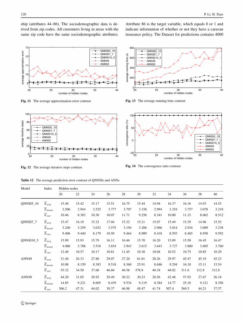
From Tables 8–11, we can see that the performance ofQNNSI5_10, QNNSI7_7 and QNNSI10_5 are obviously su-perior to that of the two ANNs. The convergence ratio ofthese three QNNSIs reaches 100% under a variety of val-ues of hidden nodes. Overall, the other three indicators ofthese three QNNSIs are better than that of two ANNs, andthere is good stability when the number of hidden nodeschanges. The same results also are illustrated in Figs. 11,12, 13 and 14.

Next, we investigate the generalization ability of QNNSI.Based on the above experimental results, we only investigateQNNSI5_10, QNNSI7_7, and QNNSI10_5. Our experimentscheme is that three QNNSIs and two ANNs are respec-tively done 10 training by the first 200 years (1749–1948)data, and are immediately tested by the remaining 59 years(1949–2007) data after each training. The average predic-tion error of the 10 tests is regarded as the evaluation index.The average prediction error contrast of QNNSIs and ANNsare shown in Table 12. Taking 35 hidden nodes for exam-ple, the average prediction result contrast are illustrated inFig. 15. The experimental results show that the generaliza-tion ability of three QNNSIs is obviously superior to that ofcorresponding ANNs.

Table 8 Training results of average approximation error

Model Hidden nodes

20 22 24 26 28 30 32 34 36 38 40

QNNSI1_50 40.20 40.20 38.60 36.60 28.90 20.30 36.90 34.90 52.80 18.00 43.40

QNNSI2_25 19.30 19.40 28.10 36.60 18.40 26.80 36.30 36.00 26.80 17.30 35.70

QNNSI5_10 12.40 12.20 10.30 10.60 9.600 10.30 11.00 9.700 10.00 9.400 8.500

QNNSI7_7 15.50 13.50 13.60 13.20 12.10 12.30 12.60 11.90 11.80 10.30 10.40

QNNSI10_5 18.00 14.80 15.70 14.50 15.60 13.80 14.60 13.40 14.10 12.80 13.40

QNNSI25_2 99.20 85.00 93.30 89.60 82.70 72.20 77.50 60.90 75.20 66.10 71.20

QNNSI50_1 100 100 100 100 100 100 100 100 100 100 100

ANN49 87.90 88.40 84.80 86.20 89.60 85.80 88.00 85.30 82.50 69.90 87.60

ANN50 79.10 92.60 93.20 79.40 92.30 87.60 85.80 86.60 92.40 76.00 87.30


Table 9 Training results of average iterative steps

Model Hidden nodes

20 22 24 26 28 30 32 34 36 38 40

QNNSI1_50 40.69 36.69 40.47 40.40 21.84 8.450 40.54 36.26 72.73 8.144 54.84

QNNSI2_25 26.38 22.84 37.13 51.01 22.57 40.84 50.82 58.47 36.96 22.61 62.47

QNNSI5_10 9.102 9.103 9.233 8.988 9.027 9.115 9.023 8.961 9.072 8.942 9.028

QNNSI7_7 9.125 9.174 9.072 9.211 9.028 8.940 9.174 8.936 9.110 8.961 9.081

QNNSI10_5 9.277 8.901 9.150 9.134 9.123 9.129 9.161 9.155 8.984 9.199 9.100

QNNSI25_2 38.02 39.66 26.08 20.55 22.83 10.97 11.88 9.875 14.43 9.276 9.636

QNNSI50_1 94.40 94.40 94.40 94.40 94.39 94.39 94.38 94.20 94.40 94.40 94.40

ANN49 10.37 10.87 10.15 10.38 10.10 9.828 10.22 9.807 9.765 9.414 9.812

ANN50 9.808 10.38 10.37 9.559 10.46 10.00 9.737 9.708 9.628 9.524 9.896

Table 10 Training results of average running time (s)

Model Hidden nodes

20 22 24 26 28 30 32 34 36 38 40

QNNSI1_50 389.30 489.90 586.80 684.20 665.30 554.70 1191.9 1344.2 2387.4 972.20 2670.7

QNNSI2_25 162.28 221.41 344.19 495.03 250.20 384.93 768.91 837.37 691.63 336.29 707.80

QNNSI5_10 113.61 105.38 92.445 104.11 114.82 150.21 150.02 137.65 149.81 143.35 152.54

QNNSI7_7 66.266 55.433 74.901 93.984 95.672 101.76 129.86 126.66 136.12 139.53 140.45

QNNSI10_5 92.259 72.502 103.34 108.26 129.73 115.09 158.92 211.05 246.20 212.38 215.31

QNNSI25_2 567.20 484.80 478.20 634.80 588.40 419.10 551.80 358.50 492.20 496.80 1283.5

QNNSI50_1 497.20 497.10 634.80 784.10 671.30 789.90 699.60 645.70 627.80 741.10 2659.4

ANN49 314.85 296.63 335.97 407.13 404.54 546.14 677.46 591.49 714.95 613.73 786.97

ANN50 106.07 156.89 197.15 207.75 293.74 334.77 390.02 465.37 578.43 553.22 742.02

Table 11 Training results of convergence ratio (%)

Model Hidden nodes

20 22 24 26 28 30 32 34 36 38 40

QNNSI1_50 80 80 80 80 90 100 80 80 60 100 70

QNNSI2_25 90 90 80 70 90 80 70 70 80 90 70

QNNSI5_10 100 100 100 100 100 100 100 100 100 100 100

QNNSI7_7 100 100 100 100 100 100 100 100 100 100 100

QNNSI10_5 100 100 100 100 100 100 100 100 100 100 100

QNNSI25_2 10 50 30 40 50 70 80 90 70 90 80

QNNSI50_1 0 0 0 0 0 0 0 0 0 0 0

ANN49 40 40 50 40 40 60 50 50 60 80 60

ANN50 80 20 30 70 30 40 60 50 60 80 50

5.3 Caravan insurance policy prediction

In this experiment, we predict who would be interestedin buying a caravan insurance policy. This data set usedin the CoIL 2000 Challenge contains information on cus-tomers of an insurance company and comes from the fol-

lowing url: http://kdd.ics.uci.edu/databases/tic/tic.html. Thedata was supplied by the Dutch data mining company Sen-tient Machine Research and is based on a real world busi-ness problem. The training set contains 5822 descriptions ofcustomers. Each record consists of 86 attributes, containingsociodemographic data (attribute 1–43) and product owner-

http://kdd.ics.uci.edu/databases/tic/tic.html

120 P. Li, H. Xiao

ship (attributes 44–86). The sociodemographic data is de-rived from zip codes. All customers living in areas with thesame zip code have the same sociodemographic attributes.

Fig. 11 The average approximation error contrast

Fig. 12 The average iterative steps contrast

Attribute 86 is the target variable, which equals 0 or 1 andindicate information of whether or not they have a caravaninsurance policy. The Dataset for predictions contains 4000

Fig. 13 The average running time contrast

Fig. 14 The convergence ratio contrast

Table 12 The average prediction error contrast of QNNSIs and ANNs


20 22 24 26 28 30 32 34 36 38 40

QNNSI5_10 Eavg 15.48 15.42 15.17 15.51 16.75 15.44 14.94 16.37 16.16 14.93 14.53

Emean 3.506 2.944 3.525 3.777 3.797 3.158 2.994 3.354 3.757 3.078 3.218

Evar 10.46 8.383 10.30 10.07 11.71 9.256 8.341 10.00 11.15 8.062 8.512

QNNSI7_7 Eavg 15.47 16.19 15.32 17.04 15.32 15.21 15.07 15.49 15.39 14.96 15.52

Emean 3.240 3.259 3.032 3.575 3.194 3.206 2.966 3.014 2.934 3.089 3.238

Evar 9.406 9.440 8.179 10.50 9.464 8.989 8.418 8.593 8.465 8.958 9.592

QNNSI10_5 Eavg 15.99 15.93 15.79 16.11 16.46 15.70 16.20 15.89 15.58 16.45 16.47

Emean 4.086 3.788 3.518 3.654 3.943 3.615 3.643 3.727 3.880 3.605 3.760

Evar 12.40 10.57 10.17 10.81 11.45 10.30 10.04 10.52 10.75 10.85 10.29

ANN49 Eavg 31.40 26.33 27.80 29.07 27.20 61.01 28.26 29.97 45.47 45.19 45.23

Emean 10.08 8.159 8.383 9.518 8.360 25.91 8.686 9.294 16.18 15.11 15.54

Evar 55.32 34.50 37.60 46.60 40.58 578.8 40.18 48.02 311.6 312.8 312.8

ANN50 Eavg 44.20 31.05 28.92 29.49 30.32 30.23 28.56 42.48 57.92 27.67 26.18

Emean 14.85 9.221 8.605 8.439 9.534 9.119 8.384 14.77 25.16 9.121 8.356

Evar 306.2 47.31 44.02 39.37 46.98 49.47 41.74 307.4 569.5 44.21 37.57


Fig. 15 The average prediction results contrast of QNNSIs and ANNs


QNNSIs ANN


1 85 85 1

5 17 85 1

17 5 85 1

85 1 85 1

customer records of whom only the organisers know if theyhave a caravan insurance policy. It has the same format asthe training set, only the target is missing. Participants aresupposed to return the list of predicted targets only.

Considering the each customer consists of 85 feature at-tributes for the input nodes and the sequence length, weemploy the four kinds of settings shown in Table 13. Inthis experiment, we set the number of hidden nodes to10,11, . . . ,20, respectively. The maximum number of itera-tive steps is set to 100. The other parameters of QNNSIs andANN are set by the same way as the previous experiment. Inthis experiment, we do not set the value of target error. Thealgorithm is not stopped until it reaches the predefined max-imum number of iterative steps.

QNNSIs and ANN train 10 times for each setting of hid-den nodes by the training set data, and are immediatelytested by the testing set data after each training. The eval-uation indicators used in this experiment are defined as fol-lows.

The number of correct prediction results Suppose y1, y2,

. . . , yM denote the desired outputs of M samples, and y1,

y2, . . . , yM denote the corresponding actual outputs, whereM denotes the number of samples in training set. The num-ber of correct prediction results for training set is definedas

Ntr =N∑

n=1

(

M −M∑

m=1

∣∣ym − [

ym]∣∣

)

/N, (41)

where N denotes the total number of training trials, ifym ≥ 0.5, then [ym] = 1, otherwise [ym] = 0. Similarly, thenumber of correct prediction results for the testing set is de-fined as

Nte =N∑

n=1

(

M −M∑

m=1

∣∣ym − [

ym]∣∣

)

/N, (42)

where M denotes the number of samples in testing set.

The ratio of correct prediction results The ratio of correctprediction results for the training set is defined as

Rtr = 100Ntr/M. (43)

Similarly, the ratio of correct prediction results for thetesting set is defined as

Rte = 100Nte/M. (44)

Then, we use these four indicators and the average run-ning time Tavg to compare QNNSIs with ANN. Experimen-tal result contrasts are shown in Table 14.

It can be seen from Table 14 that the average runningtime of QNNSI85_1 is the shortest, and so, it is the mostefficient. The Rte of QNNSI17_5 is the greatest, and so, itsgeneralization ability is the strongest. For ANN85, althoughthe Rtr is the greatest of the five models, its generalizationability is inferior to QNNSI17_5 and QNNSI5_17. In addi-tion, for the four QNNSIs, almost all of the Rte are greaterthan the corresponding Rtr , which suggests that QNNSI hasstronger generalization ability than ANN.

5.4 Breast cancer prediction

In this experiment, we give an example of predicting breastcancer with QNNSI and ANN. Features are computed froma digitized image of a fine needle aspirate (FNA) of a breastmass. They describe characteristics of the cell nuclei presentin the image. A few of the images can be found at the follow-ing url: http://www.cs.wisc.edu/~street/images/. The datasetis linearly separable using all 30 input features, and 2 predic-tion fields respectively are benign and malignant. The num-ber of instances in the dataset equals to 569, where 357 in-stances are benign and 212 instances are malignant. The bestpredictive accuracy obtained using one separating plane inthe 3-D space of Worst Area, Worst Smoothness and MeanTexture. Separating plane described above can be obtainedusing Multi-surface Method-Tree (MSM-T), a classificationmethod which uses linear programming to construct a deci-sion tree. The actual linear program used to obtain the sep-arating plane in the 3-dimensional space is that described inRef. [23]. The above-mentioned classifier has correctly di-agnosed 176 consecutive new patients as of November 1995.

http://www.cs.wisc.edu/~street/images/

122 P. Li, H. Xiao

Tabl

e14

The

perf

orm

ance

cont

rast

ofQ

NN

SIs

and

AN

Nfo

rca

rava

nin

sura

nce

polic

ypr

edic

tion

Mod

elIn

dex

Hid

den

node

s

1011

1213

1415

1617

1819

20

QN

NSI

1_85

Ntr

4837

.150

03.2

4752

.847

56.1

4891

.349

41.8

4732

.147

72.8

4864

.647

74.7

4856

.7

Rtr

(%)

83.0

8385

.937

81.6

3581

.692

84.0

1584

.881

81.2

8081

.978

83.5

5682

.011

83.4

19

Nte

3326

.134

40.5

3266

.232

68.2

3363

.433

96.0

3253

.332

82.2

3344

.432

83.2

3336

.8

Rte

(%)

83.1

5386

.012

81.6

5681

.705

84.0

8584

.900

81.3

3282

.055

83.6

0982

.081

83.4

20

Tavg

(s)

2350

824

329

2731

930

642

3394

736

282

3817

439

897

4284

244

537

4706

1

QN

NSI

5_17

Ntr

5359

.354

72.7

5243

.754

67.5

5355

.652

81.0

4612

.146

30.4

5305

.954

71.2

4454

.4

Rtr

(%)

92.0

5394

.000

90.0

6793

.911

91.9

8990

.708

79.2

1879

.533

91.1

3593

.975

76.5

10

Nte

3682

.437

61.5

3602

.337

56.1

3682

.636

27.7

3163

.631

85.0

3648

.437

59.9

3062

.6

Rte

(%)

92.0

6094

.038

90.0

5893

.903

92.0

6590

.693

79.0

9079

.625

91.2

1093

.998

76.5

65

Tavg

(s)

3254

.135

06.2

3879

.841

32.0

4586

.448

38.0

5002

.852

91.1

5518

.858

04.1

5972

.3

QN

NSI

17_5

Ntr

5302

.154

73.8

5473

.554

39.1

5474

.054

71.2

5473

.654

73.9

5474

.053

12.4

5474

.0

Rtr

(%)

91.0

7094

.019

94.0

1493

.423

94.0

2393

.975

94.0

1694

.021

94.0

2391

.247

94.0

23

Nte

3646

.237

62.0

3762

.037

31.8

3762

.037

60.8

3762

.037

62.0

3762

.036

54.1

3761

.9

Rte

(%)

91.1

5594

.050

94.0

5093

.295

94.0

5094

.020

94.0

5094

.050

94.0

5091

.353

94.0

48

Tavg

(s)

1841

.419

95.2

2148

.323

43.3

2586

.228

33.7

2939

.331

88.7

3349

.736

00.3

3719

.5

QN

NSI

85_1

Ntr

2934

.528

64.3

2868

.329

23.4

2941

.828

73.4

2979

.229

18.5

2960

.028

75.8

2920

.1

Rtr

(%)

50.0

4049

.198

49.2

6750

.213

50.5

2949

.354

51.1

7150

.129

50.8

4249

.395

50.1

56

Nte

2025

.619

78.8

1975

.120

18.5

2019

.819

80.3

2056

.919

72.0

2035

.419

88.5

2004

.9

Rte

(%)

50.6

4049

.470

49.3

7850

.463

50.4

9549

.508

51.4

2349

.300

50.8

8549

.713

50.1

23

Tavg

(s)

1590

.817

47.6

1878

.720

78.1

2300

.123

18.5

2640

.926

93.1

3009

.230

96.7

3295

.9

AN

N85

Ntr

5689

.757

15.3

5660

.756

66.8

5726

.357

35.6

5682

.957

11.8

5717

.356

87.9

5680

.9

Rtr

(%)

97.7

2898

.167

97.2

2997

.334

98.3

5698

.516

97.6

1198

.107

98.2

0297

.697

97.5

76

Nte

3612

.535

97.7

3639

.336

24.7

3586

.235

86.0

3616

.635

95.1

3591

.336

20.4

3627

.6

Rte

(%)

90.3

1389

.943

90.9

8390

.618

89.6

5589

.650

90.4

1589

.878

89.7

8390

.510

90.6

90

Tavg

(s)

1834

.319

94.2

2246

.623

32.1

2566

.128

02.1

2881

.331

30.3

3315

.035

75.6

3675

.8



QNNSIs ANN


1 30 30 1

2 15 30 1

3 10 30 1

5 6 30 1

6 5 30 1

10 3 30 1

15 2 30 1

30 1 30 1

In all samples, we use the first 400 instances (where 227are benign) to train the network, and the remaining 169 in-stances (where 130 are benign) to test the generalization ofthe proposed model. For the input nodes and the sequencelength, we employ the eight kinds of settings shown in Ta-ble 15. In this experiment, we set the number of hiddennodes to 5,6, . . . ,15, respectively. The maximum number ofiterative steps is set to 100. The other parameters of QNNSIsand ANN are set in the same way as the previous experi-ment. In this experiment, we do not set the value of the tar-get error. The algorithm is not stopped until it reaches thepredefined maximum number of iterative steps.

Our experiment scheme is below. QNNSIs and ANNtrain 10 times for each setting of hidden nodes by the train-ing set data, and are immediately tested by the testing setdata after each training. Then, we use the same evaluationindicators as the previous experiment to compare QNNSIswith ANN. Experimental contrast results are shown in Ta-ble 16.

It can be seen from Table 16 that, as far as the approxima-tion and generalization ability are concerned, QNNSI1_30and QNNSI30_1 are obviously inferior to ANN30;QNNSI2_15 and QNNSI15_2 are roughly equal to ANN30;QNNSI3_10 and QNNSI10_3 are slightly superior toANN30; QNNSI5_6 and QNNSI6_5 are obviously supe-rior to ANN30. As far as the average running time are con-cerned, QNNSI1_30, QNNSI2_15, and QNNSI3_10 are ob-viously longer than ANN30; QNNSI5_6 and QNNSI6_5are slightly longer than ANN30; QNNSI10_3, QNNSI15_2,and QNNSI30_1 are roughly equal to ANN30. Synthesiz-ing the above-mentioned two aspects, QNNSI shows betterperformance than ANN when the number of input nodes isclose to the sequence length.

Next, we theoretically explain the above experimental re-sults. Assume that n denotes the number of input nodes,q denotes the sequence length, p denotes the number of hid-den nodes, and m denotes the number of output nodes, andthe product of nq is approximately a constant.

It is clear that the number of adjustable parameters inQNNSI and ANN is the same, i.e., equals npq + pm. The

weights adjustment formula in the output layer of QNNSIand ANN is also the same. But, their parameters adjust-ment of hidden layer is completely different. The adjust-ment of hidden parameters in QNNSI is much more com-plex than that in ANN. In ANN, each hidden parame-ter adjustment only involves two derivative calculations.In QNNSI, each hidden layer parameter adjustment in-volves at least two and at most q + 1 derivative calcula-tions.

In QNNSI, when q = 1, although the number of in-put nodes is the greatest possible, the calculation of thehidden layer output and hidden parameter adjustment arealso the most simple, which directly lead to the reduc-tion of the approximation ability. When n = 1, the cal-culation of the hidden layer output is the most com-plex, which make the QNNSI have the strongest nonlin-ear mapping ability. However, at this time, the calcula-tion of hidden parameter adjustment is also very com-plex. A large number of derivative calculations can leadto the adjustment of parameters which tend to zero or in-finity. This can hinder the convergence of the training pro-cess and lead to the reduction of the approximation abil-ity. Hence, when q = 1 or n = 1, the approximation abil-ity of QNNSI is inferior to that of ANN. When n > 1 orq > 1, the approximation ability of QNNSI tends to im-prove, and under a certain condition, the approximation abil-ity of QNNSI will certainly be superior to that of ANN.The above analysis is consistent with the experimental re-sults.

In addition, what is the accurate relationship between n

and q to make QNNSI approximation ability the strongest?This problem needs further study, and usually depends onthe specific issues. Our conclusions based on experiments isas follows: when q/2 ≤ n ≤ 2q , QNNSIn_q is superior tothe ANN with nq input nodes.

It is worth pointing out that QNNSI is potentially muchmore computationally efficient than all the models refer-enced above in the Introduction section. The efficiency ofmany quantum algorithms comes directly from quantumparallelism that is a fundamental feature of many quantumalgorithms. Heuristically, and at the risk of over-simplifying,quantum parallelism allows quantum computers to evalu-ate a function f (x) for many different values of x simul-taneously. Although quantum simulation requires many re-sources in general, quantum parallelism leads to very highcomputational efficiency by using the superposition of quan-tum states. In QNNSI, the input samples have been con-verted into corresponding quantum superposition states af-ter preprocessing. Hence, as far as a lot of quantum ro-tation gates and controlled-not gates used in QNNSI areconcerned, information processing can be performed simul-taneously, which greatly improves the computational effi-ciency. Because the above four experiments are performed

124 P. Li, H. Xiao

Table 16 The performance contrast of QNNSIs and ANN for breast cancer prediction


5 6 7 8 9 10 11 12 13 14 15

QNNSI1_30 Ntr 180.8 217.0 188.1 210.5 198.2 237.2 202.7 219.5 198.2 203.0 204.9

Rtr (%) 45.20 54.25 47.03 52.63 49.55 59.30 50.68 54.88 49.55 50.75 51.23

Nte 66.00 86.60 53.00 92.70 66.20 95.30 64.60 92.40 65.60 58.30 68.40

Rte (%) 39.05 51.24 31.36 54.85 39.17 56.39 38.22 54.67 38.82 34.50 40.47

Tavg (s) 204.8 253.0 312.9 327.8 333.8 360.6 422.4 455.7 502.5 536.4 585.3

QNNSI2_15 Ntr 325.2 342.9 359.4 347.9 338.8 320.3 314.6 309.2 248.3 239.1 178.4

Rtr (%) 81.30 85.73 89.85 86.98 84.70 80.08 78.65 77.30 62.08 59.78 44.60

Nte 132.4 130.6 149.9 138.3 142.5 132.0 135.2 123.8 79.70 99.90 48.10

Rte (%) 78.34 77.28 88.70 81.83 84.32 78.11 80.00 73.25 47.16 59.11 28.46

Tavg (s) 89.33 115.7 122.5 145.1 181.6 217.2 240.0 317.1 359.6 275.8 281.8

QNNSI3_10 Ntr 378.5 366.9 378.6 392.8 392.2 378.0 356.7 378.2 369.2 360.8 362.5

Rtr (%) 94.63 91.73 94.65 98.20 98.05 94.50 89.18 94.55 92.30 90.20 90.63

Nte 148.0 136.2 148.1 161.2 156.6 158.5 143.2 145.5 151.9 151.5 138.1

Rte (%) 87.57 80.59 87.63 95.38 92.66 93.79 84.73 86.09 89.88 89.65 81.72

Tavg (s) 77.45 82.46 108.4 119.3 141.3 174.7 172.8 182.2 222.1 218.1 222.1

QNNSI5_6 Ntr 396.1 397.5 396.5 397.4 394.9 397.3 396.9 397.8 397.7 399.0 398.3

Rtr (%) 99.03 99.38 99.13 99.35 98.73 99.33 99.23 99.45 99.43 99.75 99.58

Nte 162.1 164.6 162.4 162.0 160.0 162.8 159.9 161.6 163.1 162.1 161.3

Rte (%) 95.92 97.40 96.09 95.86 94.67 96.33 94.62 95.62 96.51 95.92 95.44

Tavg (s) 51.35 63.32 69.94 86.37 110.6 118.8 137.1 134.9 170.8 172.9 214.6

QNNSI6_5 Ntr 396.5 397.8 397.7 395.5 395.7 398.0 397.4 397.4 398.0 398.0 398.0

Rtr (%) 99.13 99.45 99.43 98.88 98.93 99.50 99.35 99.35 99.50 99.50 99.50

Nte 163.4 164.0 162.4 162.8 164.4 162.0 164.9 163.9 163.4 163.8 162.4

Rte (%) 96.69 97.04 96.09 96.33 97.28 95.86 97.57 96.98 96.69 96.92 96.09

Tavg (s) 49.18 67.04 68.45 92.39 94.67 115.0 147.0 146.2 161.7 154.5 209.9

QNNSI10_3 Ntr 373.5 395.5 366.7 382.0 393.2 392.2 356.8 387.6 392.8 393.6 392.6

Rtr (%) 93.38 98.88 91.68 95.50 98.30 98.05 89.20 96.90 98.20 98.40 98.15

Nte 156.5 160.2 146.2 153.7 156.8 155.5 148.1 159.2 159.8 161.2 159.3

Rte (%) 92.60 94.79 86.51 90.95 92.78 92.01 87.63 94.20 94.56 95.38 94.26

Tavg (s) 42.44 59.02 62.93 83.88 82.65 104.3 110.5 134.6 136.1 166.8 196.0

QNNSI15_2 Ntr 278.8 247.4 348.6 276.5 360.9 368.1 360.2 356.6 341.8 393.9 375.5

Rtr (%) 69.70 61.85 87.15 69.13 90.23 92.03 90.05 89.15 85.45 98.48 93.88

Nte 126.0 121.0 147.6 111.3 151.6 158.5 156.4 153.7 150.0 162.9 162.3

Rte (%) 74.56 71.59 87.34 65.86 89.70 93.79 92.54 90.95 88.76 96.39 96.04

Tavg (s) 42.22 44.65 60.23 62.27 86.29 104.6 104.5 138.9 134.9 151.3 148.5

QNNSI30_1 Ntr 229.3 203.9 226.4 222.9 209.1 209.0 231.6 216.0 214.5 235.4 200.7

Rtr (%) 57.33 50.98 56.60 55.73 52.28 52.25 57.90 54.00 53.63 58.85 50.18

Nte 105.9 90.10 104.9 84.10 93.10 88.10 100.0 84.00 100.0 98.10 84.20

Rte (%) 62.66 53.31 62.07 49.76 55.09 52.13 59.17 49.70 59.17 58.05 49.82

Tavg (s) 42.39 45.21 63.31 63.61 86.65 86.29 115.4 112.6 140.9 150.4 176.5

ANN30 Ntr 364.6 274.1 342.0 347.4 324.8 336.6 347.4 365.9 359.2 376.4 359.2

Rtr (%) 91.15 68.53 85.50 86.85 81.20 84.15 86.85 91.48 89.80 94.10 89.80

Nte 153.7 105.7 142.9 151.6 139.7 133.7 151.9 147.8 145.6 149.1 145.8

Rte (%) 90.95 62.54 84.56 89.70 82.66 79.11 89.88 87.46 86.15 88.22 86.27

Tavg (s) 50.52 53.80 71.63 72.42 97.72 98.18 125.4 127.7 145.9 136.1 154.6


in classical computer, the quantum parallelism has not beenexplored. However, the efficient computational ability ofQNNSI is bound to stand out in future quantum com-puter.

6 Conclusions

This paper proposes a quantum-inspired neural networkmodel with sequence input based on the principle of quan-tum computing. The architecture of the proposed modelincludes three layers, where the hidden layer consists ofquantum neurons and the output layer consists of classi-cal neurons. An obvious difference from classical ANNis that each dimension of a single input sample consistsof a discrete sequence rather that a single value. The ac-tivation function of hidden layer is redesigned accordingto the principle of quantum computing. The Levenberg–Marquardt algorithm is employed for learning. With the ap-plication of the information processing mechanism of quan-tum controlled-rotation gates, the proposed model can effec-tively obtain the sample characteristics by way of breadthand depth. The experimental results reveal that a greaterdifference between input nodes and sequence length leadsto a lower performance of the proposed model than thatof the classical ANN, on the contrary, it obviously en-hances the approximation and generalization ability of theproposed model when input nodes are closer to the se-quence length. The following issues to the proposed model,such as continuity, computational complexity, and improve-ment of the learning algorithm, are subject of further re-search.

Acknowledgements We thank the three anonymous reviewers sin-cerely for their many constructive comments and suggestions, whichhave tremendously improved the presentation and quality of this paper.This work was supported by the National Natural Science Foundationof China (Grant No. 61170132).

Open Access This article is distributed under the terms of the Cre-ative Commons Attribution License which permits any use, distribu-tion, and reproduction in any medium, provided the original author(s)and the source are credited.

Appendix: The gradient calculation inLevenberg–Marquardt algorithm

According to the gradient descent algorithm in Ref. [22], thegradient of the rotation angles of the quantum rotation gatesin hidden layer and the connection weights in output layer

can be calculated as follows

⎧⎪⎪⎪⎪⎪⎪⎪⎪⎪⎪⎪⎪⎪⎪⎪⎪⎪⎪⎪⎪⎪⎨

⎪⎪⎪⎪⎪⎪⎪⎪⎪⎪⎪⎪⎪⎪⎪⎪⎪⎪⎪⎪⎪⎩

∂elk

∂hlj (tq )

= −ylk(1 − yl

k)wjk,

∂hlj (tr )

∂hlj (tr−1)

= (V ljr + V

l

jr )/(2hlj (tr )

√1 − (hl

j (tr−1))2),

∂hlj (tr )

∂θij (tr )=

⎧⎪⎪⎪⎪⎪⎪⎪⎨

⎪⎪⎪⎪⎪⎪⎪⎩

(hljr )

2(Uljr+U

ljr ) cot(θ l

i (tr )+θij (tr ))

hlj (tr )

,

j = 1,3,5, . . . ,

− (hljr )

2(Uljr+U

ljr ) tan(θ l

i (tr )+θij (tr ))

hlj (tr )

,

j = 2,4,6, . . . ,

∂hlj (tr )

∂ϕj (tr )= (h

ljr )

2(W ljr+W

ljr )

hlj (tr )

,

(45)

where

⎧⎪⎪⎪⎪⎪⎪⎪⎪⎪⎪⎪⎪⎪⎪⎪⎪⎪⎪⎪⎪⎪⎪⎪⎨

⎪⎪⎪⎪⎪⎪⎪⎪⎪⎪⎪⎪⎪⎪⎪⎪⎪⎪⎪⎪⎪⎪⎪⎩

hl

jr ={∏n

i=1 sin(θ li (tr ) + θij (tr )) j = 1,3,5, . . . ,

∏ni=1 cos(θ l

i (tr ) + θij (tr )) j = 2,4,6, . . . ,

U ljr = hl

j (tr−1)

√

1 − (hl

j (tr−1))2 sin

(2ϕj (tr )

),

Ul

jr = (1 − 2

(hl

j (tr−1))2) sin2(ϕj (tr )

),

V ljr = (

1 − 2(hl

j (tr−1))2)(

hl

jr

)2 sin(2ϕj (tr )

),

Vl

jr = 2hlj (tr−1)

(1 − 2

(h

l

jr

)2 sin2(ϕj (tr )))

×√

1 − (hl

j (tr−1))2

,

W ljr = hl

j (tr−1)

√

1 − (hl

j (tr−1))2 cos

(2ϕj (tr )

),

Wl

jr = 0.5(1 − 2

(hl

j (tr−1))2) sin

(2ϕj (tr )

).

(46)

Based on the above Eq. (45), we obtain

∂elk

∂θij (tr )= ∂el

k

∂hlj (tq)

· · · ∂hlj (tr+1)

∂hlj (tr )

∂hlj (tr )

∂θij (tr )

=

⎧⎪⎪⎪⎪⎪⎪⎪⎪⎪⎪⎪⎪⎪⎪⎪⎪⎪⎪⎪⎨

⎪⎪⎪⎪⎪⎪⎪⎪⎪⎪⎪⎪⎪⎪⎪⎪⎪⎪⎪⎩

(−ylk(1 − yl

k)wjk

∏q

s=r+1(Vljs + V

l

js)(hl

jr )2

× (Uljr + U

l

jr ) cot(θ li (tr ) + θij (tr )))

× (hl

j (tr )∏q

s=r+1 2hlj (ts)

√1 − (hl

j (ts−1))2)−1

j = 1,3,5, . . . ,

(ylk(1 − yl

k)wjk

∏q

s=r+1(Vljs + V

l

js)(hl

jr )2

× (Uljr + U

l

jr ) tan(θ li (tr ) + θij (tr )))

× (hl

j (tr )∏q

s=r+1 2hlj (ts)

√1 − (hl

j (ts−1))2)−1

j = 2,4,6, . . . ,

(47)

126 P. Li, H. Xiao

∂elk

∂ϕj (tr )= ∂el

k

∂hlj (tq)

· · · ∂hlj (tr+1)

∂hlj (tr )

∂hlj (tr )

∂ϕj (tr )

=(

−ylk

(1 − yl

k

)wjk

×q∏

s=r+1

(V l

js + Vl

js

)(h

l

jr

)2(Wl

jr + Wl

jr

))

×(

hlj (tr )

q∏

s=r+1

2hlj (ts)

√

1 − (hl

j (ts−1))2

)−1

,

(48)

where j = 1,2, . . . , p, k = 1,2, . . . ,m, r = 1,2, . . . , q ,l = 1,2, . . . ,L.

The gradient of the connection weights in the outer layercan be calculated as follows

∂elk

∂wjk

= −ylk

(1 − yl

k

)hl

j (tq). (49)

References

1. Nekoukar V, Beheshti MTH (2010) A local linear radial basisfunction neural network for financial time-series forecasting. ApplIntell 33:352–356

2. Lee H, Kim E, Pedrycz W (2012) A new selective neural networkensemble with negative correlation. Appl Intell 37:488–498

3. Park B-J, Pedrycz W, Oh S-K (2010) Polynomial-based radial ba-sis function neural networks (P-RBF NNs) and their application topattern classification. Appl Intell 32:27–46

4. Hassan YF (2011) Rough sets for adapting wavelet neural net-works as a new classifier system. Appl Intell 35:260–268

5. Kim K-j, Ahn H (2012) Simultaneous optimization of artificialneural networks for financial forecasting. Appl Intell 36:887–898

6. Tsoi AC, Back AD (1994) Locally recurrent globally feedforwardnetworks: a critical review of architectures. IEEE Trans NeuralNetw 5(2):229–239

7. Kleinfeld D (1986) Sequential state generation by model neuralnetwork. In: Proceedings of the national academy of sciences ofthe United States of America, pp 9469–9473

8. Waibel A, Hanazawa T, Hinton G, Shikano K, Lang KJ (1989)Phoneme recognition using time-delay neural networks. IEEETrans Acoust Speech Signal Process 37(3):328–339

9. Lippmann RP (1989) Review of neural network for speech recog-nition. Neural Comput 1(1):1–38

10. Moustra M, Avraamides M, Christodoulou C (2011) Artificialneural network for earthquake prediction using time series magni-tude data or seismic electric signals. Expert Syst Appl 38:15032–15039

11. Kak S (1995) On quantum neural computing. Inf Sci 83(3–4):143–160

12. Purushothaman G, Karayiannis NB (1997) Quantum neural net-work (QNN’s): inherently fuzzy feedforward neural network.IEEE Trans Neural Netw 8(3):679–693

13. Zak M, Williams CP (1998) Quantum neural nets. Int J Theor Phys37(2):651–684

14. Maeda M, Suenaga M, Miyajima H (2007) Qubit neuron accord-ing to quantum circuit for XOR problem. Appl Math Comput185(2):1015–1025

15. Gupta S, Zia RKP (2001) Quantum neural network. J Comput SystSci 63(3):355–383

16. Shafee F (2007) Neural network with quantum gated nodes. EngAppl Artif Intell 20(4):429–437

17. Li PC, Li SY (2008) Learning algorithm and application of quan-tum BP neural network based on universal quantum gates. J SystEng Electron 19(1):167–174

18. Li PC, Song KP, Yang EL (2010) Model and algorithm of neu-ral network with quantum gated nodes. Neural Netw World11(2):189–206

19. da Silva AJ, de Oliveira WR, Ludermir TB (2012) Classical andsuperposed learning for quantum weightless neural network. Neu-rocomputing 75(1):52–60

20. Gonzalez-Carrasco I, Garcia-Crespo A, Ruiz-Mezcua B, Lopez-Cuadrado JL (2011) Dealing with limited data in ballistic impactscenarios: an empirical comparison of different neural network ap-proaches. Appl Intell 35:89–109

21. Gonzalez-Carrasco I, Garcia-Crespo A, Ruiz-Mezcua B, Lopez-Cuadrado JL (2012) An optimization methodology for machinelearning strategies and regression problems in ballistic impact sce-narios. Appl Intell 36:424–441

22. Hagan MT, Demuth HB, Beale MH (1996) Neural network design.PWS Publishing Company, USA

23. Bennetta KP, Mangasariana OL (1992) Robust linear program-ming discrimination of two linearly inseparable sets. Optim Meth-ods Softw 1(1):23–34

Panchi Li received the B.S. andM.S. degrees from NortheastPetroleum University, China, in1998 and 2004, respectively, and thePh.D. degree from Harbin Instituteof Technology, China, in 2009. Cur-rently, he is a professor in the schoolof computer and information tech-nology, Northeast Petroleum Uni-versity, China. His current researchinterests include quantum neuralnetworks and quantum optimizationalgorithms.

Hong Xiao received the B.S. andM.S. degrees from NortheastPetroleum University, China, in2001 and 2004, respectively, andthen she became a teacher there.Currently, she is a Ph.D. candidatein Northeast Petroleum University,China. Her current research inter-ests include neural networks andevolutionary algorithms.

Documents

Model and algorithm of quantum-inspired neural network ... · PDF fileModel and algorithm of quantum-inspired neural ... to train the neural networks forming ... Model and algorithm