Mobility in

HSDPA

Networks

BMI paper Jeanine Schoonemann

- 2 -

Mobility in HSDPA Networks

Jeanine Schoonemann

BMI paper

Supervisor dr. Sandjai Bhulai

VU University Amsterdam

Faculty of Sciences De Boelelaan 1081a

1081 HV Amsterdam The Netherlands

January 2009

- 3 -

Preface

A part of the Business Mathematics and Informatics curriculum is to write a

BMI paper.

My supervisor Dr. Sandjai Bhulai made me enthusiastic about the subject of the influence of mobility in HSDPA networks. I want to thank him for all his support during the writing of this thesis.

Jeanine Schoonemann

Amsterdam 2009

- 4 -

Summary HSDPA, an abbreviation for High-Speed Downlink Packet Access, is the new

promising technology of the mobile telecommunications industry. But is this promise a good one? In this thesis we study the influence of mobility in

HSDPA networks. What we try to find out is if and how user velocity influences the experienced throughput.

In order to solve this problem we simulated an urban environment with one user using NS-2 with EURANE. This user had a different velocity during each

of the simulations. The velocities simulated are 3, 30, 50, 80, and 120 km/h. In a final conclusion we had to conclude that NS-2 with EURANE is not

capable enough of doing these simulations, because of the way a simulation is setup by these programs. The circumstances were too ideal to resemble

the real world. Due to these too ideal circumstances the velocity of the user had no influence on the throughput of this user.

For more research we recommend to work with a different simulator, or an extension of NS-2 and EURANE.

- 5 -

Table of Contents

Preface ......................................................................................................................................- 3 -

Summary .................................................................................................................................- 4 -

Table of Contents..................................................................................................................- 5 -

Introduction ............................................................................................................................- 7 -

Mobile Telephony Communication Protocols ..............................................................- 8 -

HSDPA...................................................................................................................................- 8 -

Network Architecture of HSDPA .............................................................................- 8 -

Starting the connection .............................................................................................- 9 -

Modulation ......................................................................................................................- 9 -

WCDMA ..........................................................................................................................- 10 -

Scheduling ....................................................................................................................- 11 -

Sending the Packet....................................................................................................- 11 -

Error Solving ................................................................................................................- 12 -

Is This Fast? .................................................................................................................- 12 -

GSM .....................................................................................................................................- 13 -

GPRS....................................................................................................................................- 13 -

UMTS ...................................................................................................................................- 14 -

Wi-Fi ....................................................................................................................................- 14 -

WiMax .................................................................................................................................- 14 -

A Comparison is Made ..................................................................................................- 15 -

Performance .................................................................................................................- 15 -

Users per Cell ..............................................................................................................- 15 -

Error Handling .............................................................................................................- 16 -

Security..........................................................................................................................- 16 -

Downlink and Uplink .................................................................................................- 16 -

Infrastructure ..............................................................................................................- 16 -

Mobile Devices.............................................................................................................- 16 -

WiMax versus HSDPA ...............................................................................................- 16 -

Simulator.....................................................................................................................- 17 -

NS-2.....................................................................................................................................- 17 -

The Underlying Channel Model .............................................................................- 18 -

The Radio Propagation Model................................................................................- 18 -

Propagation Models ...................................................................................................- 19 -

EURANE ..............................................................................................................................- 21 -

Scheduling ....................................................................................................................- 21 -

Error Model ...................................................................................................................- 23 -

Tracing ...........................................................................................................................- 23 -

Scenarios .......................................................................................................................- 25 -

- 6 -

Simulating..............................................................................................................................- 26 -

Results ................................................................................................................................- 26 -

Discussion..........................................................................................................................- 27 -

Conclusion .........................................................................................................................- 27 -

Literature ...............................................................................................................................- 28 -

Appendix A: the Headers of the Input Files .............................................................- 31 -

Appendix B: the script used to run NS-2 with EURANE .....................................- 32 -

Appendix C: the Script to Calculate the Throughput in Bytes per Second ..- 35 -

- 7 -

Introduction In a fast and mobile world, nobody wants to be restrained by wires. We want

to work in virtually every location we can think of; and not just work, but work fast. Nobody wants to wait for minutes before they finally have

downloaded the e-mail they have been waiting for. It has to happen fast, accurately and anywhere we want to. Nowadays the most commonly used wireless access technologies are WLAN

(i.e., Wi-Fi, WiMax), 2G (i.e., GSM, GPRS) and 3G (i.e., UMTS, HSDPA). Of course not all of these technologies are capable of the same things, for

instance, GSM only allows voice calls and SMS, with GPRS voice calls, SMS and MMS is possible, with UMTS also access to the World Wide Web is added to these possibilities, and finally HSDPA advances UMTS by making the

transfer rate a lot higher, which makes the access to the World Wide Web more useful. The transfer rates with HSDPA are even high enough to watch

television on a mobile device. For the providers of these technologies it is very important that their performance fits the needs and expectations of their customers. If they

cannot satisfy their customers, the customers will leave to the competitor. For this reason it is very important to be able to stipulate the performance of

these technologies. To stipulate the performance of objects that have a fixed location is not very difficult; every variable is known and has a fixed value. For moving objects

this is not the case, variables change all the time and it might happen that an object moves out of the reach of a base station. Also, every location has its

own ‘problems’ when it comes to accessibility, for example, a location outside provides better access than a location inside a building. Therefore it is interesting for providers to know how they should place their

base stations with respect to each other, in order to make sure that every user can use his mobile device at any time.

Also speed might play an important role when it comes to accessibility of mobile devices. The aim of this paper is to find out if and how the speed with which a mobile device is moving through the range of a HSDPA base station

affects the throughput of data. For telecom providers it is always useful to know what throughput they can

provide and which factors influence this throughput. When they know what influences their performance, they may also be capable of improving their performance. And better performance means not only satisfied customers,

but probably also more customers.

The first part of this paper gives an explanation on HSDPA and some other relevant wireless access technologies. Also an explanation will be given why

there has been chosen to simulate HSDPA instead of any of the other technologies. The second part will focus on the simulations and the tool used for the simulations. Finally in the third part the outcomes of the simulations

will be discussed.

- 8 -

Mobile Telephony Communication

Protocols This section starts with the explanation of the different wireless technologies mentioned in the introduction. At the end a comparison will be made between the different technologies.

HSDPA HSDPA is an abbreviation for High Speed Downlink Packet Access. It is a third generation (3G) mobile telephony communications protocol that

optimizes the current UMTS network. It improves data rates and reduces latency, which leads to a reduction of the response time [High-Speed Downlink Packet Access 2008, SearchMobileComputing.com 2007, Telecom

ABC 2005, Avidor & Mukherjee 2005, van den Berg & Litjens 2004, Charlton & Roy nd, Gessner 2005, Gruber & Knauf & Li 2004, Haichuan & Jianqiu

2005, Haider & Harris & Sirisena nd, Mäder & Staehle 2007, Sliden 2007, Taaffe 2005].

Network Architecture of HSDPA As can be seen in Figure 1, the network architecture (framework) of HSDPA

consists of multiple levels. Communication in this framework happens from layer to layer. Each layer in the model responds to service requests from the

layer above and passes on service requests to the layer below.

Figure 1. Framework of the network architecture of HSDPA [Haichuan Z, Jianqiu, W. 2005].

The main function of the lowest level layer, the physical layer, is to establish a connection and to share communication resources between the users. The

- 9 -

data link layer provides the functional and procedural means to transfer data between nodes in the network and to detect (and possibly correct) errors

that occur in the physical layer. The data link layer consists of two components: the Logical Link Control

(LLC) and the Media Access Control (MAC). Each of these components has its own function within the data link layer. The LLC determines when one frame of data ends and when the next one starts. The MAC determines who is

allowed to access the media. The network layer is the third layer of the framework; it addresses messages

and translates logical addresses and names into physical addresses. Furthermore, it also determines the route from the source to the destination node and manages traffic problems, such as switching, routing, and

controlling the congestion of data packets. The transport layer is responsible for end-to-end error recovery and flow control. The application layer is the

top level of the framework; this level is the direct interface to the network. It performs common network application services for the application processes.

Starting the Connection

When a mobile device enters the range of the base station, it starts with

sending the CQI (Current Quality Indicator) of the user to the base station, it keeps sending this information as long as it is in the range of the base station. This information is send up to 500 times per second.

The CQI is a measure that shows the signal quality from the mobile device to the base station. The transfer of the CQI happens through the Uplink High

Speed-Dedicated Physical Control Channel (HS-DPCCH). Each device regularly sends this information to the base station.

Now the base station knows the CQI of every user in its range, this value is used to decide, through an intelligent algorithm, how many resources can be made available and which modulation mode can be selected.

There are two modulation modes the base station can choose of: QPSK and 16QAM.

Modulation Modulation is the process of varying a periodic waveform (tone) in such a

way that the signal can be used to convey a message. QPSK is an abbreviation for Quadrature Phase Shift Keying and is also used

in the current UMTS network. It is a phase-modulation algorithm. Phase modulation is a version of frequency modulation in which the phase of the carrier wave is modulated to encode bits of digital information in each phase

change. Phased Shift Keying is a form of phase modulation which is accomplished by the use of a finite number of states. QPSK uses four

different states. 16QAM is an abbreviation for 16 Quadrature Amplitude Modulation. It is a modulation scheme which conveys data by changing the amplitude of two

carrier waves.

- 10 -

16QAM can, in good radio conditions, deliver more than twice as much data than QPSK, but it has a higher bit error rate, and thus a higher probability for

errors in the data. The modulation mode is stipulated by the distance of the user from the base

station. When a user is close to the base station it means that the transmission quality is good and there is little probability of errors. This means that a single user in the range of the base station, but far away

from the base station, will never receive the total data transfer speed HSDPA can provide.

Figure 2 shows a typical example of how the data rate fluctuates with the signal quality. You can see that user 1 starts with a low quality, and also receives a relatively low data rate. User 2 has, at the same point in time a

good signal quality, and also receives a relatively high data rate. The signal quality and the data rate going with these qualities fluctuates over time, this

is also what the picture shows.

Figure 2. Channelization depending on reception conditions [Lurie 2006].

WCDMA

HSDPA uses the WCDMA (wideband code division multiple access) method for multiple accesses to the air interface. This means that the signal is

distributed over the entire frequency spectrum by means of code spreading. There are fifteen codes available on the High Speed-Downlink Shared

Channel (HS-DSCH). A user can be assigned to multiple codes; in order to achieve maximal throughput a user should be assigned to all of the fifteen codes.

- 11 -

Scheduling

The distribution of the signal between the users is made by a scheduler. This scheduler bases its decisions, among other things, on channel quality,

terminal capability and code availability. There is a tradeoff in making these decisions between fairness, everybody needs to be served, and utilization of the spectrum. When only users with high quality channels would be served

that would mean that the spectrum would be very good utilized, but it would not be fair to the users with lower qualities. When you would treat every user

the same, regardless of their channel qualities, this would mean that the spectrum probably would not be utilized efficiently. The figure below shows what the distribution of the signal could look like.

Every block in time stands for a time frame of 2 ms. In the first time frame of the picture user 1 and 2 are the only users that are using the spectrum. In

the following three time frames the spectrum is divided between user 1, 2, and 3. After the fourth time frame user 2 and 3 are done and do not need the spectrum anymore. So user 1 can use the whole spectrum. In the last

time frame user 4 enters the spectrum.

Figure 3. Spectrum distribution between users [Lurie 2006].

Sending the Packet

An improvement of HSDPA with respect to the older technologies is link

adaptation; this is the ability to adapt the modulation type and the coding rate to the quality of the link. For each user the base station decides which modulation mode will be used

and assigns code(s) to this user. It also decides how many packets will be sent at the next time slot to this specific user. The user receives a message

with this information through the High Speed-Shared Control Channel (HS-SCCH). This message is sent two slots before the actual packet(s) is/are sent. The acknowledgement information is sent back to the base station

- 12 -

through the HS-DPCCH. After that, the actual data is sent to the user through the HS-DSCH.

Figure 4 shows a very simplified picture of how the users and the base station communicate. UE1 and UE2 are two users in the system, they both

send information about their signal quality, this is the L1 feedback shown in the picture. When the base station knows the quality it can decide if and how much data will be sent to each user, these are the Data arrows in the picture.

Figure 4. Communication between mobile devices and the base station [Malkowski et al. nd].

Error Solving

To solve errors made when transmitting the data HSDPA uses HARQs (hybrid

automatic repeat requests). This means that when a device detects an error in a packet, it requests this packet again at the base station. This packet is resent with a different coding, so that the device recognizes it as a resent

packet, this is called incremental redundancy. The packet with the error is saved in the buffer of the device. As soon as the packet is received by the

user, the device combines these two packets into one correct packet. So even if the resent packet contains errors, this does not mean that the packet has to be send again, it could also be the case that the packets with errors

can be combined into one packet without errors.

Is this Fast?

This all may seem a very time consuming process, and it would be with UMTS, because with UMTS a slot would be 10 ms, but with HSDPA a slot is

only 2 ms long. This makes HSDPA able to respond to changing conditions faster. This also means that the probability of an error decreases and the

time needed to repair an error decreases as well.

- 13 -

GSM GSM is an abbreviation for Global System for Mobile communication. It is the most commonly used standard for mobile communication [GSM 2008,

Halonen et al. 2003]. It is not only used for voice transfers, but also for SMS (Short Message Service) messages.

This standard uses TDMA (Time Division Multiple Access), which means that eight different callers can use the same frequency at the same time when they use the Full Rate. It is also possible to use the Half Rate, in which case

up to sixteen users can use the same frequency at the same time. Each of these users has its own time slot, so only one user can speak at a

time. But because of the speed at which this happens, users never notice that they have some time in which they cannot speak to the person on the

other end. TDMA is not really a very efficient technique, because a time slot is open for a user even when this user is not using it.

Just like HSDPA, GSM also uses a modulation technique. For GSM the used modulation technique is GMSK (Gaussian Minimum-Shift Keying), this is

some kind of FSK (Frequency Shift Keying), which first smoothes the signal with a Gaussian Low-Pass Filter and then sends it to the modulator.

GPRS GPRS (General Packet Radio Service) is a packet-oriented mobile data

service, which is often classified as 2.5G, since it is the bridge between the second and the third generation of mobile communication technologies.

GPRS is an enhancement of GSM which makes WAP access, MMS, and mobile internet services such as e-mail and the World Wide Web available to the mobile user [General Packet Radio Service 2008, Halonen et al. 2003].

The way GPRS works is quite similar to GSM technology, but because of an enhancement in the TDMA protocol it can provide a much higher data rate.

The enhancement made to the TDMA protocol as it was used for GSM, is that now a channel is only open for the user who will really use it, instead of just being open for a user, even when this is not necessary. This means that only

users that indicate they need the channel can use the channel. Users that are not in need of the channel cannot use the channel either.

This makes GPRS packet-switched, while GSM is circuit-switched. Because of this enhancement GPRS can provide a data rate from 56 up to 114 Kbits per second.

- 14 -

UMTS The architecture of UMTS (Universal Mobile Telecommunication System) is based on its predecessors GSM and GPRS. The new UMTS technology uses

these older technologies in combination with a few changes to improve the rate in which data can be transferred [Universal Mobile Telecommunications

System 2008, Kaaranen et al. 2005]. The foremost change with respect to GSM/GPRS is the different use of the air interface; UMTS uses WCDMA, just as HSDPA. This means that the air

interface is more efficiently used with UMTS than with GSM/GPRS. For the modulation, UMTS uses QPSK instead of the GSMK as used in

GSM/GPRS. QPSK is more efficient and thus has a higher data rate than GSMK.

Wi-Fi Wi-Fi is a popular wireless technology, which is used in products such as home networks, mobile phones, and video games. It is supported by almost every personal computer operating system, and by more advanced game

consolers, printers, and other peripherals [IEEE 802.11 2008, Wi-Fi 2008, Stephens 2009, Yuan 2005].

It uses the IEEE 802.11 standard; this standard contains multiple different modulation techniques which all use the same protocol. A few of the used modulation techniques are:

• DSSS (Direct-Sequence Spread Spectrum) • OFDM (Orthogonal Frequency-Division Multiplexing)

• CCK (Complementary Code Keying) • DCF (Distributed Coordination Function) • DFS (Dynamic Frequency Selection)

The protocol used here is a Carrier Sense Multiple Access with Collision Avoidance (CSMA/CA) protocol. In this protocol a station first verifies the

absence of other traffic on a shared medium. When there is no other traffic, the station sends out a signal to the other stations, telling them not to transmit, and then sends its packet of information.

Wi-Fi is very limited when it comes to the range of a base. For this reason it is most commonly used at home or in the office.

WiMax WiMax is an addition to Wi-Fi, it makes it possible to cover longer distances and connect multiple Wi-Fi stations to each other [IEEE 802.16 2008, WiMAX

Forum 2008, WiMax 2008, Blacharski nd, Goldman 2004, Gray 2006, Marks 2008]. WiMax is quite similar to Wi-Fi, but because of enhancements in the

technique, WiMax supports adaptive modulation and coding, and uses HARQs (Hybrid Automatic Repeat Requests) for good error correction performance.

WiMax can use different modulation techniques; which one to use depends on the circumstances, as with HSDPA.

- 15 -

For a good signal the highly efficient 64QAM (Quadrature Amplitude Modulation) can be used, when the signal gets poorer, also 16QAM and QPSK

(Quadrature Phase Shift Keying) can be used. For a poor signal the, very robust, BPSK (Binary Phase-Shift Keying) can be used.

A Comparison is Made Now that we know in a broad sense how each of the most used technologies work, it is time to compare them [Lurie 2006]. Next to the costs that come with each of the technologies, this comparison gives us some ammunition in

the everlasting discussion which technology should be used for mobile internet.

It is, for obvious reasons, not necessary to compare the older technologies to the newer ones. So let us just focus on the two main technologies; HSDPA

and WiMax. In order to compare them to each other, we need to know more about their performance. So let us begin by taking a closer look at how they perform.

Performance

WiMax HSDPA

Range (km) 50 35

Theoretical throughput (Mbit/s)

70 14.4

Actual throughput (Mbit/s) 5.86 3.6 (growing to 7.2)

As can be seen in the above table, WiMax seems to be the stronger one of these two technologies. But there are more issues than the ones mentioned

in the table.

Users per Cell

With HSDPA a lot of users in the same cell lead to a very low data rate. With WiMax there is a maximum number of users per cell, this is at its best a few

hundreds. When this maximum is reached the station just stops and no new users are connected. Not a very appealing idea for telecom providers; when the connection of people gets dropped, you will not get very happy

customers. An easy solution to this problem is of course putting base stations not to far apart to ensure it is very unlikely that the maximum number of

users is reached.

- 16 -

Error Handling

When it comes to error handling you will not find many differences between these two technologies, since they both use the same technology: HARQ.

Security HSDPA does not provide any additional security next to SIM authentication.

The data encoding done by the CDMA standard is quite safe, it works better than any cryptographic algorithm, but not in the case that an intruder is in a

base station or somehow gets the channel codes. WiMax does support additional security techniques, such as cryptographic algorithms, which comes as an additional security besides the encoding.

Downlink and Uplink

WiMax can offer the same downlink as uplink throughput, while HSDPA is focused on downloading and its upload speed is at best 384 Kbit/s. But this will change in the near future, since HSUPA (High Speed Uplink Packet

Access) is almost ready to become available to the customers. This makes uploading as fast as downloading.

Infrastructure HSDPA builds on the infrastructure of UMTS, which is, in The Netherlands,

already set up. This would mean that the implementation of HSDPA is more like a software upgrade. When it comes to WiMax no infrastructure is set up

yet, this would mean that a whole new structure should be designed and build.

Mobile Devices

HSDPA is already in use at the moment, but for WiMax a lot has to happen.

The first mobile devices equipped with WiMax are only expected in 2010. By that time HSDPA will already have a quite strong market position, which will make it hard for WiMax to compete. But this is the case in Western countries,

for other countries where no real infrastructure is set up yet, WiMax will probably have some advantage over HSDPA because of its performance,

range and costs; WiMax is, at this moment, much cheaper than HSDPA.

WiMax versus HSDPA

In a final conclusion it seems impossible to choose one of these two technologies as ‘the best one’. They both have their own strong and weak

points. At this point in time in The Netherlands, HSDPA has a stronger position, because it is already here and relatively easy to implement. That is why this paper is about HSDPA instead of WiMax. But who knows, in a fast

changing world as this one, it is just a matter of time before things can take an unexpected turn.

- 17 -

Simulator When it comes to problems as the one presented in this paper, simple

calculations will not do the work. There are a lot of factors involved and values change continuously; users can be moving around, signal quality

fluctuates, etc. Changing values give changing outcomes. Problems of such nature call for simulations. In a simulation a lot of different factors can be taken into account and an overview of the outcomes gives insight into the

dependencies between the factors and the quality of the communication. That is why simulation is used for the problem presented in this paper.

In order to make simulations possible, a simplified version of the real world should be used. This version of the real world should be easy enough to be implemented, but one has to be sure that no important factors are missing;

otherwise the simulation would be useless.

NS-2 For the simulations the well-known open-source discrete-event based

simulator NS-2 has been used. The reason not to write my own simulator came from the fact that the HSDPA architecture contains multiple layers, which are all needed for simulation [The Network Simulator NS-2 nd, Yuan

2005, Downard 2005, Haichuan & Jianqiu 2005]. This makes building a simulator too complex to do on your own. NS-2 can, among other things, be

used to study the performance of wireless networks. NS-2 is a hybrid of two programming languages, C++ and ObjectTcl (OTcl), Figure 5 shows a user view of NS-2.

Figure 5. User view of NS-2 [Haichuan, Z. & Jianqiu, W. 2005].

The NS-2 simulator works with an event scheduler, this scheduler picks

events from a list, actions can only happen as a result of an event. The

- 18 -

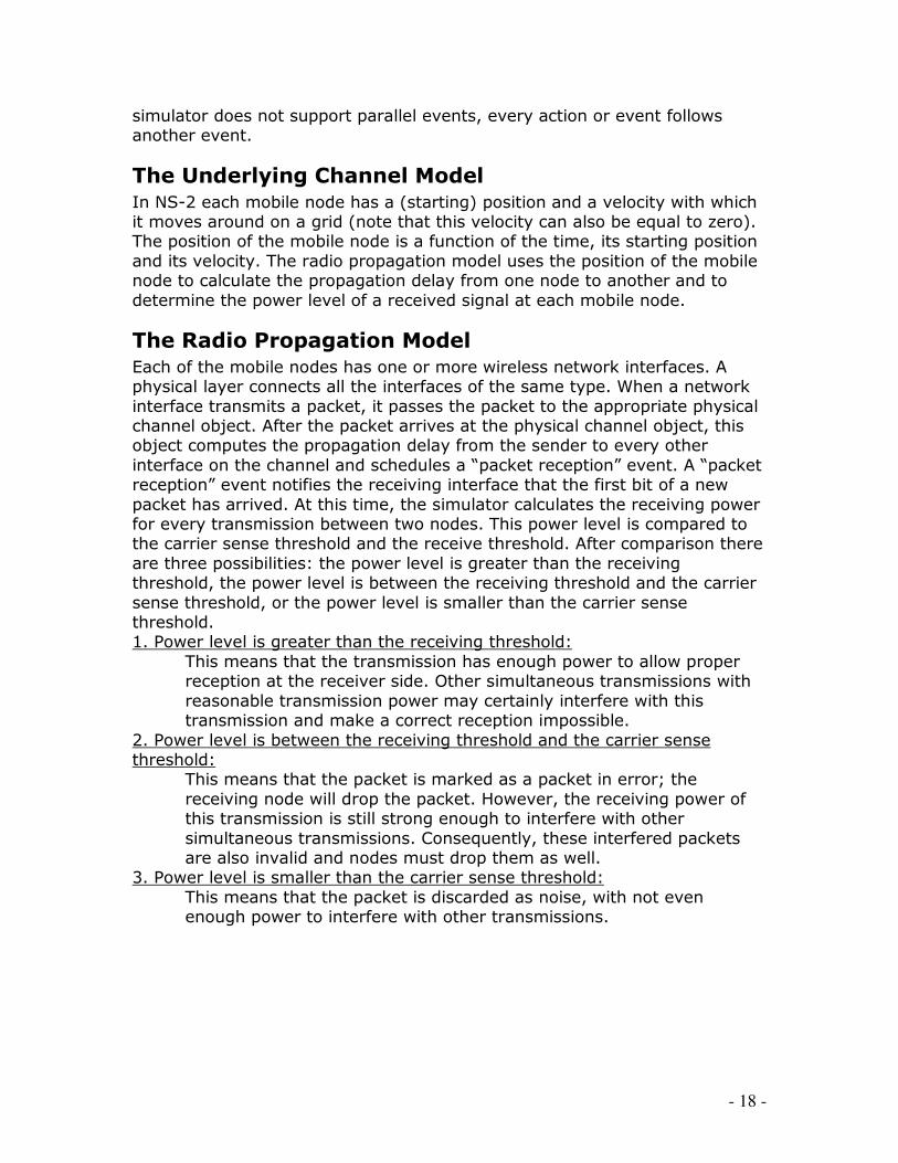
simulator does not support parallel events, every action or event follows another event.

The Underlying Channel Model

In NS-2 each mobile node has a (starting) position and a velocity with which it moves around on a grid (note that this velocity can also be equal to zero). The position of the mobile node is a function of the time, its starting position

and its velocity. The radio propagation model uses the position of the mobile node to calculate the propagation delay from one node to another and to

determine the power level of a received signal at each mobile node.

The Radio Propagation Model

Each of the mobile nodes has one or more wireless network interfaces. A physical layer connects all the interfaces of the same type. When a network

interface transmits a packet, it passes the packet to the appropriate physical channel object. After the packet arrives at the physical channel object, this object computes the propagation delay from the sender to every other

interface on the channel and schedules a “packet reception” event. A “packet reception” event notifies the receiving interface that the first bit of a new

packet has arrived. At this time, the simulator calculates the receiving power for every transmission between two nodes. This power level is compared to the carrier sense threshold and the receive threshold. After comparison there

are three possibilities: the power level is greater than the receiving threshold, the power level is between the receiving threshold and the carrier

sense threshold, or the power level is smaller than the carrier sense threshold. 1. Power level is greater than the receiving threshold:

This means that the transmission has enough power to allow proper reception at the receiver side. Other simultaneous transmissions with

reasonable transmission power may certainly interfere with this transmission and make a correct reception impossible.

2. Power level is between the receiving threshold and the carrier sense threshold:

This means that the packet is marked as a packet in error; the

receiving node will drop the packet. However, the receiving power of this transmission is still strong enough to interfere with other

simultaneous transmissions. Consequently, these interfered packets are also invalid and nodes must drop them as well.

3. Power level is smaller than the carrier sense threshold:

This means that the packet is discarded as noise, with not even enough power to interfere with other transmissions.

- 19 -

Propagation Models

To allow reasonable simulations within an acceptable amount of time, propagation models must simplify calculations and reduce the required

computation to a minimum. NS-2 knows four different propagation models to simulate wireless ad hoc networks, the Free Space (FS) model, the Two Ray Ground (TRG) model, the Shadowing model, and the Rayleigh Fading model

[Haichuan & Jianqiu 2005].

Free Space Model

The Free Space propagation model is the simplest of the three models. This model represents the range as an ideal circle, whose boundary is an absolute

limit on signal range. Furthermore this model assumes a direct path between the base station and the mobile device. The assumption is made that the nodes are in LoS (line of sight). The eventually received power depends on

multiple different system-wide constant parameters and one variable parameter. This received power is calculated by the following formula:

( ) Ld

GGPP

rtt

r

⋅⋅

⋅⋅⋅=

2

2

4π

λ,

where the system-wide constant parameters are:

Pr = the power received by the mobile device,

Pt = the power transmitted by the base station,

Gr = the gain of the antenna of the mobile device,

Gt = the gain of the antenna of the base station,

λ = the wavelength,

L = the loss coefficient of the system.

And the variable parameter is:

d = the distance between the base station and the mobile device.

As can be deduced from the formula, with the Free Space model the received power decreases as the distance to the base station increases.

- 20 -

Two Ray Ground Model

The Two Ray Ground model is an improved version of the Free Space model. As an addition to the Free Space model the Two Ray Ground model also takes the ground reflection into account as is shown in Figure 6.

Figure 6. Two Ray Ground model with a direct ray and the reflection [Gruber et al. 2004].

In the picture, ht is the height of the antenna of the base station and hr is the height of the antenna of the mobile device.

Up to a certain crossover distance, the Two Ray Ground model uses the same formula as the Free Space model, beyond this distance the ground reflection causes interference with the direct signal and further reduces the field

strength. This crossover distance can be calculated with the following formula:

dtresh = λ

πrt

hh ⋅⋅4.

This then makes the formulas used to calculate the power received:

( )

≥⋅

⋅⋅⋅⋅

<⋅⋅

⋅⋅⋅

=

tresh

rtrtt

tresh

rtt

r

ddLd

hhGGP

ddLd

GGP

P

4

22

2

2

4π

λ

Shadowing Model

The Shadowing model has a lot more variable parameters, it works with

random events. Because of this, the range does not have an absolute boundary as it was the case with the previous two models. To introduce

random events, the Shadowing model utilizes a random variable X. This random variable X has a normal distribution with an average of zero and a standard deviation σ, which is called the shadow deviation. This shadow

deviation depends on the simulated environment and is constant throughout the simulations. The values of this shadow deviation vary between three

(LoS) and twelve (outside of buildings). Furthermore, the Shadowing model requires a reference distance d0 to calculate the average received power with the Free Space model.

- 21 -

This model also works with a path loss exponent β, which, similar to the shadow deviation, depends on the simulated environment and is constant

throughout the simulations. The values of this path loss exponent β vary between two (free space) and six (indoor, non-LoS).

The formula used for the calculations is:

( )Xrtt

r

d

d

Ld

GGPP 10

4 0

2

0

2

⋅

⋅

⋅⋅

⋅⋅⋅=

−β

π

λ,

with ( ) [ ] ( ) ( ){ }2,0|,: σNxPxxX =∞∞−∈ .

Rayleigh Fading Model

On top of this Shadowing model, which gives the diffraction of the signal, the Rayleigh Fading model can be used [Rayleigh Fading, Wikipedia 2009; Sklar

1997]. You need this Rayleigh Fading model when you want to take user movements into account for the fading. Not only the distance to the base station matters, but also the velocity/movement of the user causes more

fading. The Rayleigh Fading model works a random variable R which is Rayleigh

distributed. A Rayleigh distribution is the sum of two uncorrelated Gaussian random variables. Rayleigh Fading is very useful in environments where there are a lot of objects that scatter the radio signal before this arrives at

the user. The statistical model used here is:

( )( )2

2

2

2 RE

R

re

RE

RP

−

⋅= , with random variable R ≥ 0.

EURANE EURANE is an extension of NS-2, which makes it possible to simulate HSDPA networks, something NS-2 on its own cannot be used for. EURANE extends NS-2 with three additional nodes; the Radio Network Controller (RNC), the

Base Station (BS) and the User Equipment (UE). Together these three nodes allow the support of simulating, among others, HSDPA networks. All the

features of HSDPA are there: HARQ, adaptive modulation and coding, and fast packet scheduling. This last feature, fast packet scheduling, has a few different possibilities implemented in EURANE. These possibilities will be

explained here.

Scheduling

EURANE knows three different kinds of schedulers: Round Robin, Maximum C/I, Fair Channel Dependent Scheduling (FCDS) [Malkowski et al. nd; de

Bruin et al. nd].

- 22 -

Round Robin

The Round Robin scheduling method is the fairest of the three methods. Every user gets the same number of bits transmitted in a cycle, irrespective of the channel quality. This is the fairest method as each user in the system

experiences the same average delay and throughput. But because this method does not take channel quality into account and just divides the

capacity evenly between all users, the throughput of the system is the lowest with this method.

Maximum C/I

The Maximum Carrier-to-Interface ratio method does, in contrast to Round Robin, take the channel quality into account. This method always chooses to

serve the user with the best channel conditions. This user has the highest carrier-to-interface ratio and is the most appealing to serve. This method will

obviously lead to the highest system throughput, but it is highly unfair, since users with poor channel conditions may experience big delays or may even never been served.

Fair Channel Dependent Scheduling (FCDS)

The Fair Channel Dependent Scheduling (FCDS) method is a trade-off

between the two other methods, Round Robin and Maximum C/I. The FCDS method is based on a relative power level. Practice has shown that the signal quality fluctuates in time around a mean value. FCDS takes the relative

power into account; the relative power is the instantaneous power level relative to its own recent history. The transmission level of all users is first

translated with respect to their local mean, and then normalized with their local standard deviations. A smoothing parameter is used to weight past

observations. A transmission is scheduled for the user with the lowest relative power. In this way all users get their share of the throughput of the system, no users are left out and the system is utilized in an optimal way.

When the smoothing parameter used in FCDS would be equal to zero or one, the system would be operating in extremes; a value equal to zero would lead

to a same scheduling type as the Maximum C/I method, a value equal to one would lead to a same scheduling type as the Round Robin method. The figure below gives an overview of the three methods in relation to each

other. In this figure MP stands for Maximum C/I, RR for Round Robin and FCDS for Fair Channel Dependent Scheduling.

Figure 7. Maximum C/I, Round Robin and Fair Channel Dependent Scheduling

[de Bruin et al. nd].

- 23 -

Error Model

EURANE uses a standard NS-2 channel to connect the base station to the user; in addition to this standard channel an error model is used. This

addition consists of two parts, a BLER (block error rate) performance curve and an input file of received powers and CQI. The BLER matrix is a standard matrix which can be found at the EURANE website [EURANE Website 2006],

the input file with received powers and CQI can be generated through Matlab scripts. These scripts can also be found at the EURANE website [EURANE

Website 2006].

Tracing

In order to interpret the results from a simulation EURANE and NS-2 use trace files [Haichuan & Jianqiu 2005]. The trace files from EURANE have the

following format:

Figure 8. Trace format of EURANE [Haichuan Z, Jianqiu, W. 2005].

Event: there are four types of events: enqueue (+), dequeue (-), drop (d),

and receive (r).

Time: the simulation time in seconds of the event.

From node and to node: identify the link on which the event occurred.

Pkt type: the type of the packet.

Pkt size: the size of the packet in bytes.

Flags: protocol specific information.

Fid: flow id, can be set by the user in the input script.

Src addr: the source address.

Dst addr: the destination address.

Seq num: the packet sequence number.

Pkt id: a unique packet id, necessary to trace a packet.

RLC seq: the RLC sequence number, this can be used to trace RLC packets.

- 24 -

Below is, as an example, a small part of a trace file:

+ 0.120021 1 2 UM 40 -------- 0 7.0 2.0 0 7 45

+ 0.120021 1 2 UM 40 -------- 0 7.0 2.0 0 7 46

+ 0.120022 1 2 UM 10 -------- 0 7.0 2.0 0 7 47

- 0.122 1 2 HARQ_1 185 -------- 0 7.0 2.0 0 0 0

- 0.124 1 2 HARQ_1 116 -------- 0 7.0 2.0 0 0 4

- 0.126 1 2 HARQ_1 81 -------- 0 7.0 2.0 0 1 6

- 0.128 1 2 HARQ_1 116 -------- 0 7.0 2.0 0 1 7

- 0.13 1 2 HARQ_1 157 -------- 0 7.0 2.0 0 1 9

- 0.132 1 2 HARQ_1 57 -------- 0 7.0 2.0 0 2 12

- 0.134 1 2 HARQ_2 185 -------- 0 7.0 2.0 0 0 0

r 0.134005 1 2 UM 40 -------- 0 7.0 2.0 0 0 0

r 0.134005 1 2 UM 40 -------- 0 7.0 2.0 0 0 1

r 0.134005 1 2 UM 40 -------- 0 7.0 2.0 0 0 2

r 0.134005 1 2 UM 40 -------- 0 7.0 2.0 0 0 3

r 0.134005 1 2 UM 40 -------- 0 7.0 2.0 0 0 4

r 0.134005 1 2 UM 10 -------- 0 7.0 2.0 0 0 5

As we can see in this example, in the first few lines the packets with number 45, 46, and 47 are send and put in the queue. Packet number 0 has to be resent twice, and packet numbers 4, 6, 7, 9, and 12 also are resent. In the

end we see that packet numbers 0, 1, 2, 3, 4, and 5 are received by the user.

- 25 -

Scenarios

EURANE knows multiple standard scenarios that can be used for simulation. In order to use one of these scenarios, you use the Matlab scripts provided

on the EURANE website [EURANE Website 2006]. When running these scripts you can choose between fourteen different scenarios.

1. Single Rayleigh Channel,

2. Single Rayleigh Channel w/o correlation on fading coefficients,

3. Case 1,

4. Case 2,

5. Case 3,

6. Indoor Office A,

7. Indoor Office B,

8. Pedestrian A,

9. Pedestrian B,

10.Vehicular A,

11.Vehicular B,

12.Rural Area,

13.Typical Urban,

14.Hilly Terrain.

Each scenario has four variables: velocity of the user(s), distance to the base

station, trace length, and number of users. With these scenarios EURANE provides an easy way to test different kinds of

environments, such as an indoor office, a pedestrian or a user in a vehicle. Each of these scenarios use the Rayleigh Fading model, the difference between the scenarios can be found in the parameters used for this Rayleigh

Fading model.

- 26 -

Simulating For the simulation the Typical Urban scenario (scenario 13) has been used,

with different user speeds while keeping the other variables constant. The values chosen for the other variables are as follows:

Distance to the base station – 500 meter, Trace length – 1200 seconds, Number of users – 1 user.

For the velocity of the user a few different values have been used: 3 km/h,

30 km/h, 50 km/h, 80 km/h, and 120 km/h. These velocities differ from a pedestrian user, who is walking around with a velocity of 3 km/h, to a user who is driving on the freeway in his car with a velocity of 120 km/h.

As has been said before, EURANE uses the Rayleigh Fading method.

The scheduling methods that were looked at before are variable in EURANE; in the script used to run NS-2 with EURANE a choice can be made as to which

scheduling method has to be used in the simulation. In our case we only work with one user, and because of that there is no need to use a scheduling

method, since the total system throughput will be used by one and the same user.

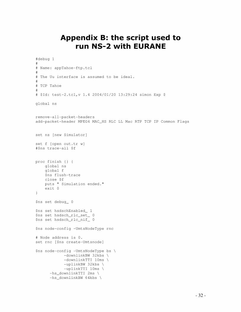
After creating the input file with the above values, the simulation can start. To show which decisions were made, the header of the input files can be

found in Appendix A, the speed is left blank in this header, because this was variable during the simulations. For these simulations a BLER (block error rate) matrix and the input file are used, together with a script to run NS-2

with EURANE. This script can be found in Appendix B, it has been taken almost directly from the EURANE website [EURANE Website 2006], only the

simulation time has been changed.

Results In order to interpret the results of the simulations, the resulting trace files

were read through a script. This script can be found in Appendix C. With the help of this script the throughput in bytes per second could be calculated for each simulation. The final results of the simulation are shown in the following

figure.

- 27 -

Throughput in bytes/second

3000

3500

4000

4500

0 20 40 60 80 100 120

Velocity

Bytes/second

Figure 9. The throughput in bytes per second.

Discussion The figure shows that the throughput almost does not change as the velocity

of the user changes; this is in line with what was expected from the literature [Lun, X. 1995]. But it is not what one would expect when looking at the real world. When looking at the simulations performed it becomes clear where

this gap between the simulations and the real world comes from. In the simulations the user never leaves the cell, so the simulation only takes place

in one cell. In this cell the user drives in a circle around the base station, staying at exactly the same distance from the base station the whole time. Circumstances seem to be too ideal to really cover what would happen in the

real world. When driving through multiple cells, users have to connect to different base stations and encounter interference from these base stations.

The simulation of this scenario, however, falls outside the scope of this paper and is left as future research.

Conclusion In a final conclusion it can be said that NS-2 with EURANE is not fit yet to

simulate the problem presented in this paper. At this moment it is possible to simulate multiple cells with NS-2 and EURANE, but this is still in a startup

phase and no conclusions can be drawn from these simulations yet. For more research it is recommended to work with a simulator that can, reliably, simulate a multi-cell HSDPA network with user movements that

resemble the real world; someone driving in exact circles around the base station is not realistic. When this is possible a reliable simulation can be done

for this problem, which may eventually lead to a reliable model of the influence of user movements in a HSDPA network.

- 28 -

Literature EURANE Website 2006, viewed 6 January 2009,

<http://eurane.ti-wmc.nl/eurane/>.

General Packet Radio Service, Wikipedia 2008, 25 August 2008, viewed 31 August 2008, <http://en.wikipedia.org/wiki/GPRS>, <http://nl.wikipedia.org/wiki/GPRS>.

GSM, Wikipedia 2008, 18 August 2008, viewed 30 August 2008,

<http://en.wikipedia.org/wiki/GSM>, <http://nl.wikipedia.org/wiki/GSM>. High-Speed Downlink Packet Access, Wikipedia 2008, 15 August 2008,

viewed 30 August 2008, <http://en.wikipedia.org/wiki/Hsdpa>, <http://nl.wikipedia.org/wiki/Hsdpa>

IEEE 802.11, Wikipedia 2008, 30 August 2008, viewed 31 August 2008, <http://en.wikipedia.org/wiki/802.11>,

<http://nl.wikipedia.org/wiki/802.11>.

IEEE 802.16, Wikipedia 2008, 29 August 2008, viewed 31 August 2008, <http://en.wikipedia.org/wiki/802.16>, <http://nl.wikipedia.org/wiki/802.16>.

Rayleigh Fading, Wikipedia 2009, 9 November 2008, viewed 6 January 2009,

<http://en.wikipedia.org/wiki/Rayleigh_fading>. SearchMobileComputing.com 2007, TechTarget, Needham, USA, viewed 31

August 2008, <http://searchmobilecomputing.techtarget.com/sDefinition/0,,sid40_gci1218

632,00.html>, <http://searchmobilecomputing.techtarget.com/sDefinition/0,,sid40_gci213688,00.html>.

Telecom ABC 2005, Telecom ABC, viewed 31 August 2008,

<http://www.telecomabc.nl/h/hsdpa.html>, <http://www.telecomabc.nl/u/umts.html>.

The Network Simulator NS-2 nd, viewed 7 January 2009, <http://www.isi.edu/nsnam/ns/>

Universal Mobile Telecommunications System, Wikipedia 2008, 24 August

2008, viewed 31 August 2008, <http://en.wikipedia.org/wiki/UMTS>, <http://nl.wikipedia.org/wiki/UMTS>.

Wi-Fi, Wikipedia 2008, 28 August 2008, viewed 31 August 2008, <http://en.wikipedia.org/wiki/WiFi>, <http://nl.wikipedia.org/wiki/Wi-Fi>.

- 29 -

WiMAX Forum 2008, WiMAX Forum, Beaverton, USA, viewed 31 August

2008, <www.wimaxforum.org>. WiMAX, Wikipedia 2008, 12 July 2008, viewed 30 August 2008,

<http://en.wikipedia.org/wiki/WiMAX>, <http://nl.wikipedia.org/wiki/WiMAX>.

Avidor, D. & Mukherjee, S. 2005. Downlink Dimensioning for the HSDPA Standard. Wireless Personal Communications, 32 (139-152)

Berg, H. van den & Litjens, R. & Laverman, J. 2004. HSDPA Flow Level Performance: The Impact of Key System and Traffic Aspects.

Blacharski, D. nd, What is WiMax?, viewed 31 August 2008,

<http://www.wisegeek.com/what-is-wimax.htm>. Bruin, I. de & Heijenk, G & El Zarki, M. & Lei Zan, J (nd). Fair Channel-

Dependent Scheduling in CDMA Systems.

Charlton, G. & Roy, V. (nd). Link-to-System Interface for Estimating HSDPA System Performance for Interference Mitigating Receivers.

Downard, I. 2004. Simulating Sensor Networks in NS-2.

Gessner, C. (October 2005). A UMTS Booster. Telecommunications International, 39, 10 (30-31)

Goldman, J. 2004, HSDPA vs. WiMax, viewed 31 August 2008, <http://www.wi-fiplanet.com/news/article.php/3434341>.

Gray, D. (September 2006). Mobile WiMAX: A Performance and Comparative

Summary. Gruber, I. & Knauf, O. & Li, H. 2004. Performance of Ad Hoc Routing

Protocols in Urban Environments.

Haichuan, Z. & Jianqiu, W. 2005. Implementation and Simulation of HSDPA Functionality with NS-2.

Haider, A. & Harris, R. & Sirisena, H. (nd). Simulation-Based Performance Analysis of HSDPA for UMTS Networks.

Halonen T. & Romero, G. & Romero, J. & Melero, J. 2003. GSM, GPRS and EDGE Performance: Evolution Towards 3G/UMTS, John Wiley and Sons.

Kaaranen, H. & Ahtiainen, A. & Laitinen, L. & Naghian, S. & Niemi, V. 2005.

UMTS Networks: Architecture, Mobility and Services, John Wiley and Sons.

- 30 -

Lun, X. 1995. Adaptive Threshold Controlling Scheme for AMC Binding in HSDPA.

Lurie, S. 2006, HSDPA vs. WiMAX: Comparing Characteristics and Prospects

of Datacom Technologies, viewed 6 January 2009, <http://www.digit-life.com/articles2/mobile/wimax.html>. Mäder, A. & Staehle, D. 2007. A Flow-Level Simulation Framework for

HSDPA-enabled UMTS Networks.

Malkowski, M. & Kemper, A. & Wang, X. (nd). Performance of Scheduling Algorithms for HSDPA.

Marks, R.B. 2008, The IEEE 802.16 Working Group on Broadband Wireless Access Standards, viewed 6 January 2009, <http://ieee802.org/16/>.

Plewes, A. 2006. HSDPA: 3G Saviour? Telecommunications International, 40, 2 (13-16).

Sklar, B. July 1997. Rayleigh Fading Channels in Mobile Digital

Communication Systems Part I: Characterization. IEEE Communications Magazine, (90-100).

Sliden, F. nd, What is HSDPA?, viewed 31 August 2008, <http://www.wisegeek.com/what-is-hsdpa.htm>.

Stephens, Adrian 2009, IEEE 802.11 Then Working Group Setting the

Standards for Wireless LANs, viewed 6 January 2009, <http://ieee802.org/11/>.

Taaffe, O. 2005. HSDPA: High-Speed Data of Potential Attrition? Telecommunications International, 39, 10 (11)

Taaffe, O. 2005. HSDPA on the Way? Telecommunications International, 39, 6 (21-23)

Taaffe, O. (February 2005). What’s the 3G Attraction? Telecommunications

International, 39, 2 (16-18) Yuan, T. (June 2005). Performance Modeling and Analysis of Mobile Internet

Access via Cellular Networks.

- 31 -

Appendix A: the Headers of the Input Files %%%%%%%%%%%%%%%%%%%%%%%%%%%%%%%%%%%%%%%%%%%%%%%%%%%%%%%%%%%%%%%%%%%%%%%

%%

% Number of comment lines: 31

% Tracefile generated at: 11-Nov-2008 11:03:56

% in directory: H:\MATLAB

% with file name: output/Urban-3kmh-500m-1200s-UEnr1

% by: 'whoami' is not recognized as an internal or

external command,

operable program or batch file.

% containing: P, P_1stRT, P_2ndRT, CQI

% i.e. P(t), MRC{P(t),P(t+H)}, MRC{P(t),P(t+H),P(t+2*H)}, CQI(.. P(t-

D).. )

% with MRC=Maximum Ratio Combining technique

% with H=HARQcycle= 6

% and D=CQIdelayinTTI= 3

% with trace length (numTTItrace): 600000

% corresponding time interval in seconds: 1200

% (Note that this is the time between stop and finish for the event

% scheduler in ns-2, which is longer than the time interval of the

source)

% for user #: 1

% velocity (km/h): ……………………………

% distance (m) from BS: 500.00000000

% which environment (nr,name): 13 Urban environment

% BS Transmission power (dBm): 38

% Base station antenna gain (in dBi): 17

% Linit (distance loss at 1 km): 1.374000e+002

% Iintra (intra cell interference): 30

% Iinter (inter cell interference): -70

% HARQ cycle period: 6

% Time delay (TTI) in CQI: 3

% Minimum CQI value: 0

% Maximum CQI value: 30

% Percentage of adapted (too low) CQI values: 3

% Percentage of adapted (too high) CQI values: 0

%%%%%%%%%%%%%%%%%%%%%%%%%%%%%%%%%%%%%%%%%%%%%%%%%%%%%%%%%%%%%%%%%%%%%%%

%%

- 32 -

Appendix B: the script used to

run NS-2 with EURANE #debug 1

#

# Name: appTahoe-ftp.tcl

#

# The Uu interface is assumed to be ideal.

#

# TCP Tahoe

#

# $Id: test-2.tcl,v 1.4 2004/01/20 13:29:24 simon Exp $

global ns

remove-all-packet-headers

add-packet-header MPEG4 MAC_HS RLC LL Mac RTP TCP IP Common Flags

set ns [new Simulator]

set f [open out.tr w]

#$ns trace-all $f

proc finish {} {

global ns

global f

$ns flush-trace

close $f

puts " Simulation ended."

exit 0

}

$ns set debug_ 0

$ns set hsdschEnabled_ 1

$ns set hsdsch_rlc_set_ 0

$ns set hsdsch_rlc_nif_ 0

$ns node-config -UmtsNodeType rnc

# Node address is 0.

set rnc [$ns create-Umtsnode]

$ns node-config -UmtsNodeType bs \

-downlinkBW 32kbs \

-downlinkTTI 10ms \

-uplinkBW 32kbs \

-uplinkTTI 10ms \

-hs_downlinkTTI 2ms \

-hs_downlinkBW 64kbs \

- 33 -

# Node address is 1.

set bs [$ns create-Umtsnode]

$ns setup-Iub $bs $rnc 622Mbit 622Mbit 15ms 15ms DummyDropTail 2000

$ns node-config -UmtsNodeType ue \

-baseStation $bs \

-radioNetworkController $rnc

# Node address for ue1 and ue2 is 2 and 3, respectively.

set ue1 [$ns create-Umtsnode]

set ue2 [$ns create-Umtsnode]

# Node address for sgsn0 and ggsn0 is 4 and 5, respectively.

set sgsn0 [$ns node]

set ggsn0 [$ns node]

# Node address for node1 and node2 is 6 and 7, respectively.

set node1 [$ns node]

set node2 [$ns node]

$ns duplex-link $rnc $sgsn0 622Mbit 0.4ms DropTail 1000

$ns duplex-link $sgsn0 $ggsn0 622MBit 10ms DropTail 1000

$ns duplex-link $ggsn0 $node1 10MBit 15ms DropTail 1000

$ns duplex-link $node1 $node2 10MBit 35ms DropTail 1000

$rnc add-gateway $sgsn0

set tcp0 [new Agent/UDP]

$tcp0 set fid_ 0

$tcp0 set prio_ 2

$ns attach-agent $node2 $tcp0

#$ns attach-agent $rnc $tcp0

set ftp0 [new Application/Traffic/CBR]

$ftp0 attach-agent $tcp0

set sink0 [new Agent/Null]

$sink0 set fid_ 0

$ns attach-agent $ue1 $sink0

$ns connect $tcp0 $sink0

$ns node-config -llType UMTS/RLC/UM \

-downlinkBW 64kbs \

-uplinkBW 64kbs \

-downlinkTTI 20ms \

-uplinkTTI 20ms \

-hs_downlinkTTI 2ms \

-hs_downlinkBW 64kbs

$ns create-hsdsch $ue1 $sink0

$bs setErrorTrace 0 "idealtrace"

$bs setErrorTrace 1 "idealtrace"

- 34 -

$bs loadSnrBlerMatrix "SNRBLERMatrix"

#set dch0 [$ns create-dch $ue1 $sink0]

$ue1 trace-inlink $f 1

$bs trace-outlink $f 1

$rnc trace-inlink-tcp $f 0

$rnc trace-outlink $f 2

# tracing for all hsdpa traffic in downtarget

$rnc trace-inlink-tcp $f 0

$bs trace-outlink $f 2

# per UE

$ue1 trace-inlink $f 2

$ue1 trace-outlink $f 3

$bs trace-inlink $f 3

$ue1 trace-inlink-tcp $f 2

$ns at 0.0 "$ftp0 start"

$ns at 1000.0 "$ftp0 stop"

$ns at 1000.401 "finish"

puts " Simulation is running ... please wait ..."

$ns run

- 35 -

Appendix C: the Script to Calculate the

Throughput in Bytes per Second BEGIN {

recv = 0

flow = 0

flow_t = UM

hdr_size = 0

dst = 2

simtime = 1000

}

{

# Trace line format: normal

if ($2 != "-t") {

event = $1

time = $2

if (event == "+" || event == "-") node_id = $3

if (event == "r" || event == "d") node_id = $4

flow_id = $8

pkt_id = $12

pkt_size = $6

}

# Trace line format: new

if ($2 == "-t") {

event = $1

time = $3

node_id = $5

flow_id = $39

pkt_id = $41

pkt_size = $37

}

# Calculate total received packets' size

if (flow_id == flow && event == "r" && node_id == dst) {

if (flow_t != "sctp") {

recv += pkt_size - hdr_size

#printf("recv[%g] = %g --tot:

%g\n",node_id,pkt_size-hdr_size,recv)

} else {

# Rip off SCTP header, whose size depends

# on the number of chunks in each packet

if (pkt_size != 448 && pkt_size != 864 &&

pkt_size != 1280) pkt_size = 0

if (pkt_size == 448) pkt_size = 400

if (pkt_size == 864) pkt_size = 800

if (pkt_size == 1280) pkt_size = 1200

recv += pkt_size

#printf("recv[%g] = %g --tot:

%g\n",node_id,pkt_size,recv)

}

}

}

END {

printf("%10g %10s %10g\n",flow,flow_t,(recv/simtime)*(8/1000))

}