Mobile robots kinematics - Chromechrome.ws.dei.polimi.it/.../Robotics_03_Mobile_Robots_Kinematics.pdf · Mobile robots kinematics Matteo Matteucci –[email protected]

Mobile robots kinematicsMatteo Matteucci – [email protected]

Matteo Matteucci – [email protected]

2Mobile robots classification

Wheeled robots

• Kind of wheels

• Kinematics

• Odometry

Legged robots

• Number of legs

• Type of joints

• Stability

• Coordination

Whegs

• ???


3Wheeled Mobile Robots

A robot capable of locomotion on a surface solely through the actuation of wheel assemblies mounted on the robot and in contact with the surface. A wheel assembly is a device which provides or allows motion between its

mount and surface on which it is intended to havea single point of rolling contact.

(Muir and Newman, 1986)

Robot Mobile AGV Unmanned vehicle


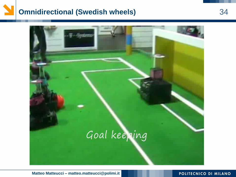
4Wheels types

x

y

FixedOrientable

centered

Caster

omnidirectional

Swedish or

Meccanum


5Mobile robots types (some)

Two wheels (differential drive)

• Simple model

• Suffers terrain irregularities

• Cannot translate laterally

Tracks

• Suited for outdoor terrains

• Not accurate movements (with rotations)

• Complex model

• Cannot translate laterally

Omnidirectional (synchro drive)

• Can exploit all degrees of freedom (3DoF)

• Complex model

• Complex structure


6Differential drive


7Differential drive


8Omnidirectional (Swedish wheels)


9Omnidirectional (Syncro drive)


10Degrees of freedom and holonomy

The degrees of freedom are the variables needed to characterize

the position of a body in space (a.k.a. Maneuverability)

• Differential drive has DOF=3

• Omnidirectional robot has DOF=3

The differentiable degrees of freedom (DDoF) are robot

independently achievable velocities

• Differential drive has DDoF=2

• Omnidirectional robot has DDoF=3

We can have different constraints to the motion

• Holonomic kinematic constraints can be expressed as an explicit

function of position variables

• Non-holonomic constraints can be expressed as differential

relationship, such as the derivative of a position variable

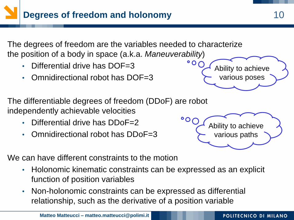
Ability to achieve

various poses

Ability to achieve

various paths


11Kinematic constraints

Constraints can be expressed as a set of equations/disequations of position

and velocity of the points in the system

Ψ(… , 𝑃𝑖 , 𝑃𝑖 , … , 𝑡) ≥ 0

Holonomic (position) constraints have no dependence on the velocity

• They subtract a degree of freedom for each constraint equation

Non holonomic (mobility) constraints restrict only the velocity

• They allow to reach any position

• They do not reduce the degrees of freedom

• Some paths are not allowed while any position can be reached

(e.g., with a car, whilst it is possible for it to be in any

position on the road, it is not possible for it to move sideways)


12

s

Holonomic constraint example

Let’s consider a rolling cylinder without slipping

• 6 coordinates, x, y, z, φ, ψ, ϑ

• 5 constraints:

• z=0, since it rolls on the plane

• s = (x2 + y2)1/2, space covered replaces 2 coordinates with 1

• φ = constant, since we have no slippage

• ψ = 0, the plane faces are orthogonal to the plane

• s’ = r ϑ’, i.e., ds= r d if the cylinder rolls without slipping

• The latter becomes an additional holonomic constrain: s-s0= r (ϑ - ϑ 0)

• Only 1 degree of mobility (6 – 5), i.e., s (or ϑ)

Can go only

straigth!

ϑ


13Non holonomic constraint example

Let’s consider a thin disk rolling on an horizontal plane

• 6 coordinates, x, y, z, φ, ψ, ϑ

• 4 constraints:

• z=0, since it rolls on the plane

• s = (x2 + y2)1/2, space covered replaces 2 coordinates with 1

• ψ = 0, the plane faces are orthogonal to the plane

• s’ = r ϑ’, i.e., ds= r d if the disk rolls without slipping

• It can spin about both ϑ (roll) and, φ (turn)

so the latter is non holonomic

• 3 degrees of mobility (6 – 3), i.e., φ + s + ϑ

ϑ

φ

Can go

everywhere!

Can follow

any path!


15Some definitions ...

Locomotion: the process of causing an autonomous robot to move

• To produce motion, forces must be applied to the vehicle

Dynamics: the study of motion in which forces are modeled

• Includes the energies and speeds associated with these motions

Kinematics: study of motion without considering forces that affect if

• Deals with the geometric relationships that govern the system

• Deals with the relationship between control parameters and the

behavior of a system in state space

We’ll focus on

this one!We’ll stick on

the plane!


16Kinematics

Direct kinematics

• Given control parameters, e.g., wheels and velocities, and a time of

movement t, find the pose (x, y, ) reached by the robot

Inverse kinematics

• Given the final pose (x, y, ) find control parameters to move the robot

there in a given time t

Direct

kinematics:

integrating

. . .

x(t), y(t), (t)

Inverse

kinematics

wheels parameters

wheels parameters

robot pose:

x(t), y(t), (t)

control variables:

angular velocity (t)

linear velocity (t)


17Wheeled robot assumptions

1. Robot made only by rigid parts

2. Each wheel may have a 1 link for steering

3. Steering axes are orthogonal to soil

4. Pure rolling of the wheel about its axis (x axis)

5. No translation of the wheel

y

roll

z motion

x

y

Wheel parameters:

r = radius

v = linear velocity

= angular velocity


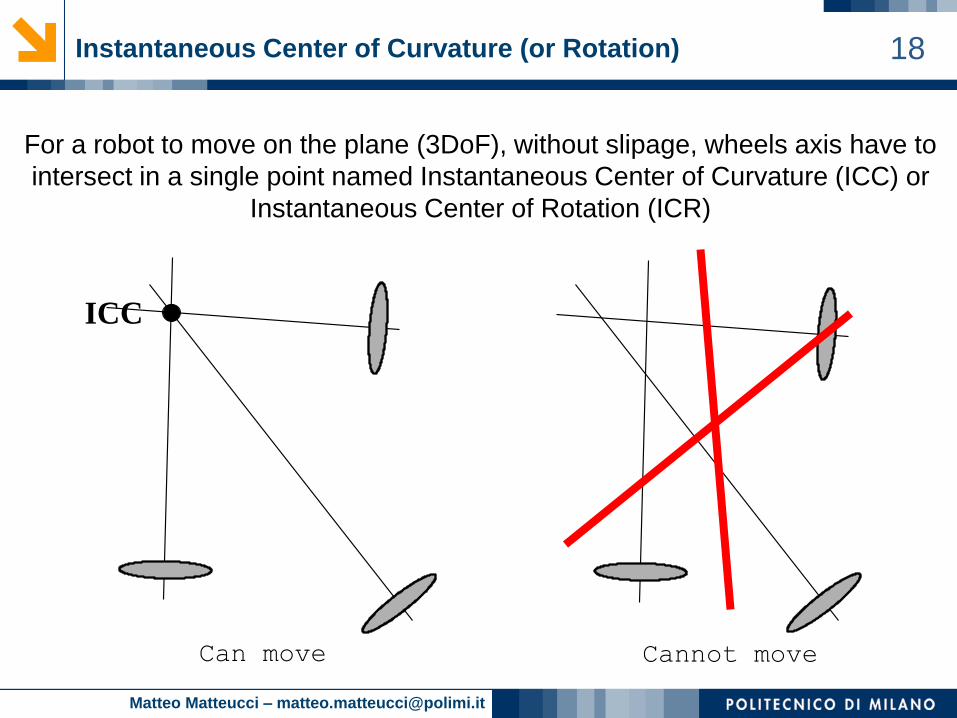
18Instantaneous Center of Curvature (or Rotation)

For a robot to move on the plane (3DoF), without slipage, wheels axis have to

intersect in a single point named Instantaneous Center of Curvature (ICC) or

Instantaneous Center of Rotation (ICR)

ICC

Cannot moveCan move


19

(xb, yb) base

reference frame

Representing a pose

xb

yb

xm

ym

ICC

(xm, ym) robot

reference frame

Rotation is

around the zm axis

𝑃 = 𝑥𝑏 , 𝑦𝑏, 𝜃 = 𝑥, 𝑦, 𝜃


20

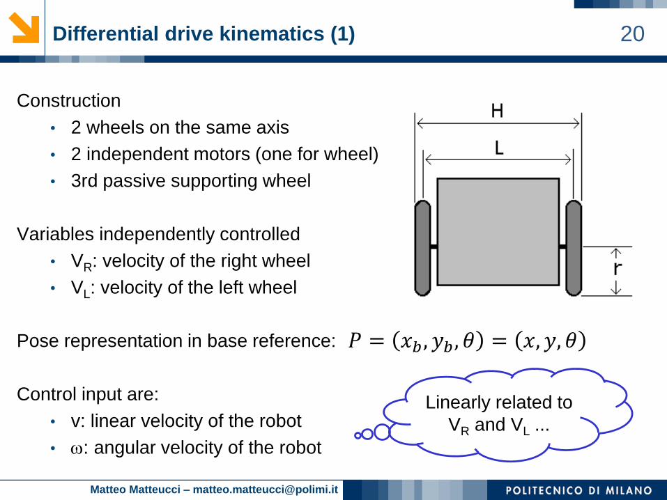
Construction

• 2 wheels on the same axis

• 2 independent motors (one for wheel)

• 3rd passive supporting wheel

Variables independently controlled

• VR: velocity of the right wheel

• VL: velocity of the left wheel

Pose representation in base reference:

Control input are:

• v: linear velocity of the robot

• : angular velocity of the robot

Differential drive kinematics (1)

𝑃 = 𝑥𝑏 , 𝑦𝑏, 𝜃 = 𝑥, 𝑦, 𝜃

Linearly related to

VR and VL ...


21

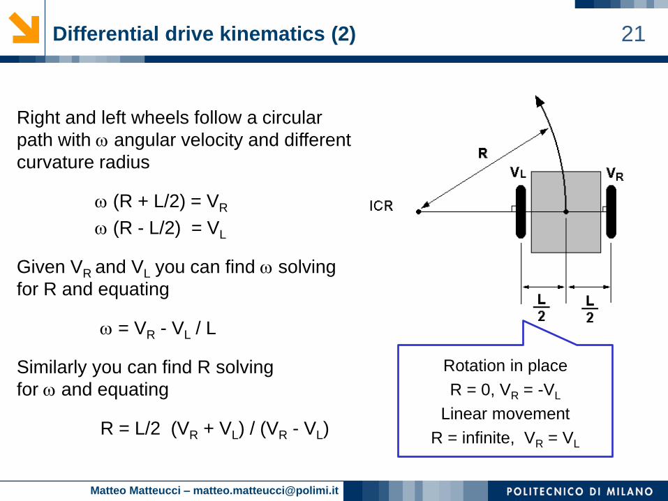
Right and left wheels follow a circular

path with angular velocity and different

curvature radius

(R + L/2) = VR

(R - L/2) = VL

Given VR and VL you can find solving

for R and equating

= VR - VL / L

Similarly you can find R solving

for and equating

R = L/2 (VR + VL) / (VR - VL)

Differential drive kinematics (2)

Rotation in place

R = 0, VR = -VL

Linear movement

R = infinite, VR = VL


22Differential drive ICC

Wheels move around ICC on a

circumference with istantaneous

radius R and angular velocity

ICC = (x+R cos( +/2), y+R sin( +/2)=

(x – R sin(), y + R cos())

ICC

R

ICC

R

P(t)

P(t+dt)

t

ICCy

ICCx

tt

tt

y

x

y

x

y

x

d

dd

dd

ICC

ICC

100

0)cos()sin(

0)sin()cos(

'

'

'

Translate

robot in ICCRotate around

ICC

Translate

robot back


23Differential drive equations (to remember!)

R

ICC

(x,y)

y

L/2

x

VL

VR

L

VV

VVV

VV

VVLR

LRV

LRV

LR

LR

LR

LR

L

R

2

)(

)(

2

)2/(

)2/(

))cos(),sin(( RyRxICC


24Differential drive direct kinematics

Being know

Compute the velocity in the base frame

Integrate position in base frame

ICR

R

Vx = V(t) cos ((t))

Vy = V(t) sin ((t))

x(t) = ∫ V(t) cos ((t)) dt

y(t) = ∫ V(t) sin ((t)) dt

(t) = ∫ (t) dt

= ( VR - VL ) / L

R = L/2 ( VR + VL ) / ( VR - VL )

V = R = ( VR + VL ) / 2

'))'()'((1

)(

'))'(sin())'()'((2

1)(

'))'(cos())'()'((2

1)(

0

0

0

t

LR

t

LR

t

LR

dttVtVL

t

dtttVtVty

dtttVtVtx

Can integrate

at discrete time


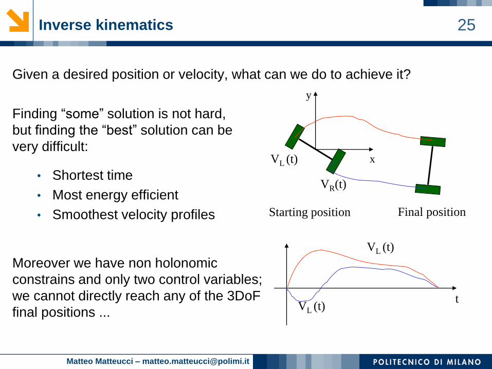
25Inverse kinematics

Given a desired position or velocity, what can we do to achieve it?

Finding “some” solution is not hard,

but finding the “best” solution can be

very difficult:

• Shortest time

• Most energy efficient

• Smoothest velocity profiles

Moreover we have non holonomic

constrains and only two control variables;

we cannot directly reach any of the 3DoF

final positions ...

VR(t)

VL (t)

Starting position Final position

x

y

VL (t)

tVL (t)


26Non holonomic constraint

The equations of the direct kinematics describe a constraint on the

velocity of the robot that cannot be integrated into a positional constraint

(non holonomic constraint):

• The robot moves on a circle

passing for (0,0) at time 0 and

(x,y) at time t

• Infinite admissible solutions

exists, but we want a specific

• No independent control of

is possible

Nevertheless a straightforward solution

exists if we limit the class of control

functions for VR and VL …

0,0,0

x,y,t


27Differential drive inverse kinematics

Decompose the problem and control only few DoF at the time

1. Turn so that the wheels are parallel

to the line between the original

and final position of robot origin

2. Drive straight until the robot’s

origin coincides with destination

3. Rotate again in to achieve the

desired final orientation

VR(t)

VL (t)

Starting position Final position

x

y

-VL (t) = VR (t) = Vmax

VL (t) = VR (t) = Vmax

-VL (t) = VR (t) = Vmax

VL (t)

tVR (t)


28Vehicles with tracks

Vehicles with track have a kinematics

similar to the differential drive

• Speed control of each track

• Use the height of the track as

wheel diameter

• Often named Skid Steering

Need proper calibration and slippage modeling


29Synchronous drive

Complex mechanical robot design

• (At least) 3 wheels actuated and steered

• A motor to roll all the wheels,

a second motor to rotate them

• Wheels point in the same direction

• It is possible to control directly

Robot control variables

• Linear velocity v(t)

• Angular velocity (t)

Its ICC is always at the infite and the robot is holonomic


30Synchronous drive kinematics

Robot control for the synchronous drive

• Direct control of v(t) and (t)

• Steering changes the direction of ICC

Particular cases:

• v(t)=0, (t) = for dt → robot rotates in place

• v(t)=v, (t) = 0 for dt → robot moves linearly

Compute the velocity in the base frame

Integrate position in base frame to get

the robot odometry (traversed path) ...

x

y v(t)

')'()(

')]'(sin[)'()(

')]'(cos[)'()(

0

0

0

t

t

t

dttt

dtttvty

dtttvtx

Vx = V(t) cos ((t))

Vy = V(t) sin ((t))

Calles odometry

also for diff drive!


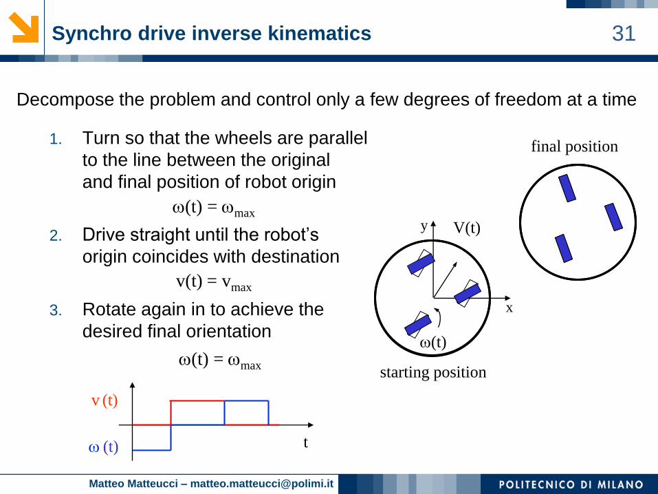
31Synchro drive inverse kinematics

Decompose the problem and control only a few degrees of freedom at a time

1. Turn so that the wheels are parallel

to the line between the original

and final position of robot origin

2. Drive straight until the robot’s

origin coincides with destination

3. Rotate again in to achieve the

desired final orientation

V(t)

(t)

starting position

final position

x

y

(t) = max

v(t) = vmax

(t) = max

v (t)

t (t)


32Omnidirectional (Syncro drive)


33

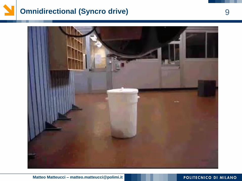
Simple mechanical robot design

• (At least) 3 Swedish wheels actuated

• One independent motor per wheel

• Wheels point in different direction

• It is possible to control directly x, y,


• Linear velocity v(t) (each component)

• Angular velocity (t)

Omnidirectional robot


34Omnidirectional (Swedish wheels)


35Tricycle kinematics

The Tricycle is the typical kinematics of AGV

• One actuated and steerable wheel

• 2 additional passive wheels

• Cannot control independently

• ICC must lie on the line that passes

through the fixed wheels


• Steering direction (t)

• Angular velocity of steering wheel (t)

Particular cases:

• (t)=0, (t) = → moves straight

• (t)=90, (t) = → rotates in place



Direct kinematics can be derived as:

In the robot frame

𝑟 = 𝑠𝑡𝑒𝑒𝑟𝑖𝑛𝑔 𝑤ℎ𝑒𝑒𝑙 𝑟𝑎𝑑𝑖𝑢𝑠

𝑉𝑠(𝑡) = 𝜔𝑠 𝑡 ∙ 𝑟

𝑅 𝑡 = 𝑑 ∙ tan(𝜋

2− 𝛼(𝑡))

𝜔 𝑡 =𝜔𝑠 𝑡 ∙ 𝑟

𝑑2 + 𝑅 𝑡 2=𝑉𝑠 𝑡

𝑑sin 𝛼 𝑡

Angular

velocity of the

moving frame

𝑉𝑥(𝑡) = 𝑉𝑠(𝑡) ∙ cos 𝛼(𝑡)

𝑉𝑦 (𝑡) = 0

𝜃 =𝑉𝑠 𝑡

𝑑∙ sin 𝛼(𝑡)

We assume

no slipage

Linear velocity

v(t)

Angular

velocity (t)



Direct kinematics can be derived as:

In the world frame

𝑟 = 𝑠𝑡𝑒𝑒𝑟𝑖𝑛𝑔 𝑤ℎ𝑒𝑒𝑙 𝑟𝑎𝑑𝑖𝑢𝑠

𝑉𝑠(𝑡) = 𝜔𝑠 𝑡 ∙ 𝑟

𝑅 𝑡 = 𝑑 ∙ tan(𝜋

2− 𝛼(𝑡))

𝜔 𝑡 =𝜔𝑠 𝑡 ∙ 𝑟

𝑑2 + 𝑅 𝑡 2=𝑉𝑠 𝑡

𝑑sin 𝛼 𝑡

𝑥 𝑡 = 𝑉𝑠 𝑡 ∙ cos 𝛼 𝑡 ∙ cos 𝜃 𝑡 = 𝑉(𝑡) ∙ cos 𝜃 𝑡

𝜃 =𝑉𝑠 𝑡

𝑑∙ sin 𝛼 𝑡 = 𝜔(𝑡)

𝑦 𝑡 = 𝑉𝑠 𝑡 ∙ cos 𝛼 𝑡 ∙ sin 𝜃 𝑡 = 𝑉(𝑡) ∙ s𝑖𝑛 𝜃 𝑡


38Ackerman steering

Most diffused kinematics on the planet

• Four wheels steering

• Wheels have limited

turning angles

• No in-place rotation

Similar to the Trycicle model

Derive the rest as:

VBL

VBR

VFR

VFL

x

y

ICC

R

L

R

d

bb

𝑅 =𝑑

tan𝛼𝑅+ 𝑏

𝜔𝑑

sin 𝛼𝑅= 𝑉𝐹𝑅 Determines angular

velocity (t)

𝜔𝑑

sin 𝛼𝐿= 𝑉𝐹𝐿 𝜔 𝑅 − 𝑏 = 𝑉𝐵𝑅𝜔 𝑅 + 𝑏 = 𝑉𝐵𝐿𝛼𝐿 = tan−1(

𝑑

𝑅 + 𝑏)


39Ackerman steering (bycicle approximation)

Most diffused kinematics on the planet

• Four wheels steering

• Wheels have limited

turning angles

• No in-place rotation

Bycicle approximation

Referred to the center of real wheels

VBL

VBR

VFR

VFL

x

y

ICC

R

L

R

d

bb

𝑅 =𝑑

tan𝛼

𝜔𝑑

sin 𝛼= 𝑉𝐹

𝜔𝑅 = 𝑉 𝜔 = 𝑉 ∙tan𝛼

𝑑

VF

V


40Mobile robots beyond the wheels

To move on the ground

• Multiple wheels

• Whegs

• Legs

To move in water

• Torpedo-like (single propeller)

• Bodies with thrusters

• Bioinspired

To move in air

• Fixed wings vehicles

• Mobile wings vehicles

• Multi-rotors

Documents

Mobile robots kinematics - Chromechrome.ws.dei.polimi.it/.../Robotics_03_Mobile_Robots_Kinematics.pdf · Mobile robots kinematics Matteo Matteucci –[email protected]