Embed Size (px)
Citation preview

Mobile Robot NavigationUsing
Active Vision
Andrew John DavisonKeble College
Robotics Research GroupDepartment of Engineering Science
University of Oxford
Submitted February 14 1998; Examined June 9th 1998.
This thesis is submitted to the Department of Engineering Science, University of Oxford,for the degree of Doctor of Philosophy. This thesis is entirely my own work, and, except
where otherwise indicated, describes my own research.

Andrew John Davison Doctor of PhilosophyKeble College Hilary Term, 1998
Mobile Robot Navigation
Using
Active Vision
Abstract
Active cameras provide a navigating vehicle with the ability to fixate and track featuresover extended periods of time, and wide fields of view. While it is relatively straightforwardto apply fixating vision to tactical, short-term navigation tasks, using serial fixation on asuccession of features to provide global information for strategic navigation is more involved.However, active vision is seemingly well-suited to this task: the ability to measure featuresover such a wide range means that the same ones can be used as a robot makes a widerange of movements. This has advantages for map-building and localisation.
The core work of this thesis concerns simultaneous localisation and map-building fora robot with a stereo active head, operating in an unknown environment and using pointfeatures in the world as visual landmarks. Importance has been attached to producing mapswhich are useful for extended periods of navigation. Many map-building methods fail onextended runs because they do not have the ability to recognise previously visited areasas such and adjust their maps accordingly. With active cameras, it really is possible tore-detect features in an area previously visited, even if the area is not passed through alongthe original trajectory. Maintaining a large, consistent map requires detailed informationto be stored about features and their relationships. This information is computationallyexpensive to maintain, but a sparse map of landmark features can be handled successfully.We also present a method which can dramatically increase the efficiency of updates inthe case that repeated measurements are made of a single feature, permitting continuousreal-time tracking of features irrespective of the total map size.
Active sensing requires decisions to be made about where resources can best be applied.A strategy is developed for serially fixating on different features during navigation, makingthe measurements where most information will be gained to improve map and localisationestimates. A useful map is automatically maintained by adding and deleting features toand from the map when necessary.
What sort of tasks should an autonomous robot be able to perform? In most applica-tions, there will be at least some prior information or commands governing the requiredmotion and we will look at how this information can be incorporated with map-buildingtechniques designed for unknown environments. We will make the distinction betweenposition-based navigation, and so-called context-based navigation, where a robot manoeu-vres with respect to locally observed parts of the surroundings.
A fully automatic, real-time implementation of the ideas developed is presented, and avariety of detailed and extended experiments in a realistic environment are used to evaluatealgorithms and make ground-truth comparisons.
1

Acknowledgements
First of all, I’d like to thank to my supervisor David Murray for all of his ideas, encour-agement, excellent writing tips and general advice — another physics recruit successfullyconverted.
Next thanks must go to Ian Reid, in particular for applying his in-depth hacking skillsto getting the robot hardware to work and leading the lab on its path to Linux gurudom.I’m very grateful to all the other past and present members of the Active Vision Lab who’vehelped daily with all aspects of my work including proof-reading, and been great companyfor tea breaks, pub trips, dinners, parties, hacky-sacking and all that: Jace, Torfi, John,Lourdes, Phil, Stuart, Eric, Nobuyuki, Paul, and Kevin. Thanks as well to all the otherRobotics Research Group people who’ve been friendly, helpful, and inspiring with their highstandard of work (in particular thanks to Alex Nairac for letting me use his robot’s wheeland David Lee for lending me a laser).
Three and a bit more years in Oxford have been a great laugh due to the friends I’vehad here: house members Ian, Julie, John, Alison, Jon, Nicky, Ali, Naomi and Rebecca,frisbee dudes Siew-li, Luis, Jon, Erik, Clemens, Martin, Gill, Bobby, Jochen, Del, Derek,squash players Dave, Raja and Stephan and the rest.
Thanks a lot to my old Oxford mates now scattered around the country for weekendsaway, holidays and email banter: Ahrash, Phil, Rich, Vic, Louise, Clare, Ian, Amir andTim; and to my friends from Maidstone Alex, Jon and Joji.
Last, thanks to my mum and dad and bruv Steve for the financial assistance, weekendsat home, holidays, phone calls and everything else.
I am grateful to the EPSRC for funding my research.
2
Contents
1 Introduction 11.1 Autonomous Navigation . . . . . . . . . . . . . . . . . . . . . . . . . . . . . 1
1.1.1 Why is Navigation So Difficult? (The Science “Push”) . . . . . . . . 11.1.2 Uses of Navigating Robots (The Application “Pull”) . . . . . . . . . 21.1.3 The Mars Rover . . . . . . . . . . . . . . . . . . . . . . . . . . . . . 41.1.4 This Thesis . . . . . . . . . . . . . . . . . . . . . . . . . . . . . . . . 5
1.2 Major Projects in Robot Navigation . . . . . . . . . . . . . . . . . . . . . . 51.2.1 INRIA and Structure From Motion . . . . . . . . . . . . . . . . . . . 61.2.2 The Oxford Autonomous Guided Vehicle Project . . . . . . . . . . . 91.2.3 MIT: Intelligence Without Representation . . . . . . . . . . . . . . . 101.2.4 Carnegie Mellon University: NavLab . . . . . . . . . . . . . . . . . . 11
1.3 Active Vision . . . . . . . . . . . . . . . . . . . . . . . . . . . . . . . . . . . 121.3.1 Previous Work in Active Vision . . . . . . . . . . . . . . . . . . . . . 13
1.4 This Thesis: Navigation Using Active Vision . . . . . . . . . . . . . . . . . 161.4.1 Some Previous Work in Active Visual Navigation . . . . . . . . . . . 161.4.2 A Unified Approach to Navigation with Active Vision . . . . . . . . 16
2 The Robot System 182.1 System Requirements . . . . . . . . . . . . . . . . . . . . . . . . . . . . . . 18
2.1.1 System Composition . . . . . . . . . . . . . . . . . . . . . . . . . . . 192.2 A PC/Linux Robot Vision System . . . . . . . . . . . . . . . . . . . . . . . 20
2.2.1 PC Hardware . . . . . . . . . . . . . . . . . . . . . . . . . . . . . . . 202.2.2 Operating System . . . . . . . . . . . . . . . . . . . . . . . . . . . . 21
2.3 The Active Head: Yorick . . . . . . . . . . . . . . . . . . . . . . . . . . . . . 222.4 The Vehicle: GTI . . . . . . . . . . . . . . . . . . . . . . . . . . . . . . . . . 232.5 Image Capture . . . . . . . . . . . . . . . . . . . . . . . . . . . . . . . . . . 242.6 Software . . . . . . . . . . . . . . . . . . . . . . . . . . . . . . . . . . . . . . 242.7 Working in Real Time . . . . . . . . . . . . . . . . . . . . . . . . . . . . . . 252.8 Calibration . . . . . . . . . . . . . . . . . . . . . . . . . . . . . . . . . . . . 25
3 Robot Models and Notation 273.1 Notation . . . . . . . . . . . . . . . . . . . . . . . . . . . . . . . . . . . . . . 27
3.1.1 Vectors . . . . . . . . . . . . . . . . . . . . . . . . . . . . . . . . . . 273.1.2 Reference Frames . . . . . . . . . . . . . . . . . . . . . . . . . . . . . 283.1.3 Rotations . . . . . . . . . . . . . . . . . . . . . . . . . . . . . . . . . 28
3.2 Camera Model . . . . . . . . . . . . . . . . . . . . . . . . . . . . . . . . . . 293.3 Active Head Model . . . . . . . . . . . . . . . . . . . . . . . . . . . . . . . . 31

3.3.1 The Head Centre . . . . . . . . . . . . . . . . . . . . . . . . . . . . . 313.3.2 Reference Frames . . . . . . . . . . . . . . . . . . . . . . . . . . . . . 323.3.3 Using the Model . . . . . . . . . . . . . . . . . . . . . . . . . . . . . 34
3.4 Vehicle Model . . . . . . . . . . . . . . . . . . . . . . . . . . . . . . . . . . . 373.4.1 Moving the Robot . . . . . . . . . . . . . . . . . . . . . . . . . . . . 373.4.2 Errors in Motion Estimates . . . . . . . . . . . . . . . . . . . . . . . 38
4 Vision Tools, and an Example of their Use 414.1 Scene Features . . . . . . . . . . . . . . . . . . . . . . . . . . . . . . . . . . 41
4.1.1 Detecting Features . . . . . . . . . . . . . . . . . . . . . . . . . . . . 424.1.2 Searching For and Matching Features . . . . . . . . . . . . . . . . . 444.1.3 Other Feature Types . . . . . . . . . . . . . . . . . . . . . . . . . . . 46
4.2 Fixation . . . . . . . . . . . . . . . . . . . . . . . . . . . . . . . . . . . . . . 474.2.1 Acquiring Features . . . . . . . . . . . . . . . . . . . . . . . . . . . . 474.2.2 The Accuracy of Fixated Measurements . . . . . . . . . . . . . . . . 48
4.3 An Example Use of Vision Tools: The Frontal Plane and Gazesphere . . . . 504.3.1 The 8-Point Algorithm for a Passive Camera . . . . . . . . . . . . . 524.3.2 The 8-Point Algorithm in The Frontal Plane . . . . . . . . . . . . . 544.3.3 The 8-Point Algorithm in the Gazesphere . . . . . . . . . . . . . . . 57
4.4 Conclusion . . . . . . . . . . . . . . . . . . . . . . . . . . . . . . . . . . . . 60
5 Map Building and Sequential Localisation 615.1 Kalman Filtering . . . . . . . . . . . . . . . . . . . . . . . . . . . . . . . . . 61
5.1.1 The Extended Kalman Filter . . . . . . . . . . . . . . . . . . . . . . 625.2 Simultaneous Map-Building and Localisation . . . . . . . . . . . . . . . . . 63
5.2.1 Frames of Reference and the Propagation of Uncertainty . . . . . . . 635.2.2 Map-Building in Nature . . . . . . . . . . . . . . . . . . . . . . . . . 65
5.3 The Map-Building and Localisation Algorithm . . . . . . . . . . . . . . . . 665.3.1 The State Vector and its Covariance . . . . . . . . . . . . . . . . . . 665.3.2 Filter Initialisation . . . . . . . . . . . . . . . . . . . . . . . . . . . . 665.3.3 Moving and Making Predictions . . . . . . . . . . . . . . . . . . . . 675.3.4 Predicting a Measurement and Searching . . . . . . . . . . . . . . . 675.3.5 Updating the State Vector After a Measurement . . . . . . . . . . . 685.3.6 Initialising a New Feature . . . . . . . . . . . . . . . . . . . . . . . . 695.3.7 Deleting a Feature . . . . . . . . . . . . . . . . . . . . . . . . . . . . 705.3.8 Zeroing the Coordinate Frame . . . . . . . . . . . . . . . . . . . . . 70
5.4 Experiments . . . . . . . . . . . . . . . . . . . . . . . . . . . . . . . . . . . . 715.4.1 Experimental Setup . . . . . . . . . . . . . . . . . . . . . . . . . . . 715.4.2 Characterisation Experiments A1 and A2 . . . . . . . . . . . . . . . 735.4.3 Experiment B: An Extended Run . . . . . . . . . . . . . . . . . . . . 795.4.4 Experiments C1 and C2: The Advantages of Carrying the Full Co-
variance Matrix . . . . . . . . . . . . . . . . . . . . . . . . . . . . . . 845.5 Conclusion . . . . . . . . . . . . . . . . . . . . . . . . . . . . . . . . . . . . 88
ii
6 Continuous Feature Tracking, and Developing a Strategy for Fixation 896.1 Continuous Tracking of Features . . . . . . . . . . . . . . . . . . . . . . . . 906.2 Updating Motion and Structure Estimates in Real Time . . . . . . . . . . . 91
6.2.1 Situation and Notation . . . . . . . . . . . . . . . . . . . . . . . . . 926.2.2 Prediction and Update . . . . . . . . . . . . . . . . . . . . . . . . . . 936.2.3 Updating Particular Parts of the Estimated State Vector and Covari-
ance Matrix . . . . . . . . . . . . . . . . . . . . . . . . . . . . . . . . 956.2.4 Multiple Steps . . . . . . . . . . . . . . . . . . . . . . . . . . . . . . 976.2.5 Summary . . . . . . . . . . . . . . . . . . . . . . . . . . . . . . . . . 100
6.3 A Strategy for Fixation: Selecting Which Feature to Track . . . . . . . . . 1036.3.1 Choosing from Known Features . . . . . . . . . . . . . . . . . . . . . 1046.3.2 Choosing New Features . . . . . . . . . . . . . . . . . . . . . . . . . 1066.3.3 Continuous Switching of Fixation . . . . . . . . . . . . . . . . . . . . 110
6.4 Conclusion . . . . . . . . . . . . . . . . . . . . . . . . . . . . . . . . . . . . 113
7 Autonomous Navigation 1167.1 Maintaining a Map . . . . . . . . . . . . . . . . . . . . . . . . . . . . . . . . 1177.2 Controlling the Robot’s Motion . . . . . . . . . . . . . . . . . . . . . . . . . 119
7.2.1 Steering Control . . . . . . . . . . . . . . . . . . . . . . . . . . . . . 1197.2.2 Road-Following by Visual Servoing . . . . . . . . . . . . . . . . . . . 122
7.3 Automatic Position-Based Navigation . . . . . . . . . . . . . . . . . . . . . 1237.3.1 Using Odometry Only . . . . . . . . . . . . . . . . . . . . . . . . . . 1237.3.2 Using Vision . . . . . . . . . . . . . . . . . . . . . . . . . . . . . . . 124
7.4 Fully Autonomous Navigation . . . . . . . . . . . . . . . . . . . . . . . . . . 1277.4.1 Incorporating Known Features into Map-Building . . . . . . . . . . . 1287.4.2 Finding Areas of Free Space . . . . . . . . . . . . . . . . . . . . . . . 1307.4.3 The Link with Context-Based Navigation . . . . . . . . . . . . . . . 1337.4.4 Conclusion . . . . . . . . . . . . . . . . . . . . . . . . . . . . . . . . 135
8 Conclusions 1378.1 Contributions . . . . . . . . . . . . . . . . . . . . . . . . . . . . . . . . . . . 1378.2 Future Work . . . . . . . . . . . . . . . . . . . . . . . . . . . . . . . . . . . 138
iii
1Introduction
1.1 Autonomous Navigation
Progress in the field of mobile robot navigation has been slower than might have beenexpected from the excitement and relatively rapid advances of the early days of research [65].As will be described later in this chapter, the most successful projects have operated inhighly constrained environments or have included a certain amount of human assistance.Systems where a robot is acting independently in complicated surroundings have often beenproven only in very limited trials, or have not produced actions which could be thought ofas particularly “useful”.
1.1.1 Why is Navigation So Difficult? (The Science “Push”)
It is very interesting to consider why autonomous navigation in unknown surroundings issuch a difficult task for engineered robots — after all, it is something which is taken forgranted as easy for humans or animals, who have no trouble moving through unfamiliarareas, even if they are perhaps quite different from environments usually encountered.
The first thing to note is the tendency of the designers of navigation algorithms toimpose methods and representations on the robot which are understandable by a humanoperator. Look at the inner workings of most map building algorithms for example (theone in this thesis included), and there is a strong likelihood of finding Cartesian (x, y, z)representations of the locations of features. It is not clear that this is the best way to dothings on such a low level, or that biological brains have any similar kind of representationdeep within their inner workings. However, having these representations does provide hugebenefits when we remember that most robots exist to perform tasks which benefit humans.It makes it simple to input information which is pertinent to particular tasks, to supervise

1.1 Autonomous Navigation 2
operation when it is necessary, and, especially in the development stage of a robotic project,to understand the functioning of the algorithm and overcome any failures.
There has been a move away from this with methods such as genetic algorithms andartificial neural networks, in which no attempt is made to understand the inner workings ofthe processing behind a robot’s actions. These methods are clearly appealing in that theyseem to offer the closest analogue with the workings of the brains behind navigation systemsin nature. The algorithms in a way design themselves. However, as described above, thisapproach creates robots which are inherently more difficult to interface with, possessing“minds of their own” to some extent.
Researchers have come up with a variety of successful modules to perform certain navi-gation tasks: for instance, to produce localisation information, to identify local hazards orto safely round a known obstacle. Joining these into complete systems has proved to bedifficult, though. Each algorithm produces its own output in a particular form and has itsown type of representation. For example, a free-space detection algorithm may generate agridded representation of the areas filled by free space or obstacles in the vicinity of a robot:how should this be used to generate reference features to be used by a close-control techniquefor safe robot guidance? Alternatively, if a robot is engaged in a close-control manoeuvre,when is it time to stop and switch back to normal operation? One of the most originalapproaches to such problems lies with the methodology of “intelligence without representa-tion” [14] put forward by Brooks and colleagues at MIT. In their systems, different modesof operation and sensing (behaviours) run concurrently in a layered architecture and votetowards the overall robot action while avoiding attempting to communicate representationsbetween themselves. This will be looked at in more detail later.
The final, very important, point is that the physical construction of robots which arerobust and reliable to standards anywhere approaching living bodies is extremely challeng-ing. Problems with batteries or the restrictions imposed by an umbilical connection to anexternal power source in particular have meant that robots are commonly not running forlong enough periods for decent evaluation of their performance and correction of their faults.Also, the complications of programming and communicating with a computer mounted ona robot and all of its devices make progress inevitably slow.
In summary, the answer to the question in the title of this section would seem to be thatthe complexity of the “real world”, even in the simplified form of an indoor environment, issuch that engineered systems have not yet come anywhere near to having the wide range ofcapabilities to cope in all situations. It does not appear that some kind of general overallalgorithm will suffice to guide a robot in all situations, and evidence shows that this is notthe case with biological navigation systems [74] which operate as a collection of specialisedbehaviours and tricks. Of course humans and animals, who have been subject to the processof evolution while living in the real world, have necessarily developed all the tricks requiredto survive.
1.1.2 Uses of Navigating Robots (The Application “Pull”)
How much is there really a need for autonomous mobile robots in real-world applications? Itis perhaps difficult to think of situations where autonomous capabilities are truly essential.It is frequently possible to aid the robot with human control, or to allow it to operateonly under restricted circumstances. High-profile systems such as the Mars Rover or road-

1.1 Autonomous Navigation 3
following cars, which will be described later, fall into these categories.Useful [71] mobile robots could then clearly be autonomous to different degrees, their
navigational capabilities depending on the application. Consider for example a device suchas an automatic vacuum cleaner or lawnmower, prototypes of both of which have been builtcommercially. Either of these operates in a well defined region (a particular room or lawn)and needs to be able to identify the limits of that region and avoid other potential hazardswhile carrying out its task. However, at least in the current designs, it does not have tohave any ability to calculate its location in the region or to plan particular paths aroundit — the behaviour pattern of both devices is a random wandering (with the addition ofan initial relatively simple edge-following stage in the case of the vacuum cleaner). Intheory they could be greatly improved in terms of efficiency if they were able to measurethe room or lawn and then plan a neat path to cover the area effectively — however, thiswould present a substantial additional challenge which is not necessarily justified. Thelawnmower in particular is designed to run purely from solar power with the idea that itcould run continuously over the lawn during the day (a kind of robotic sheep).
In other circumstances, it may be necessary for a robot to monitor its position accuratelyand execute definite movements, but possible to facilitate this in a simple way with externalhelp such as a prior map with landmark beacons in known positions. In a factory orwarehouse, where mobile robots are employed to fetch and carry, this is the obvious solution:for example, carefully placed barcode-type beacons can be scanned by a laser mounted on therobot. Robots making large movements through outdoor environments, such as unmannedfull-scale vehicles, can make use of the satellite beacons of the Global Positioning Systemto achieve the same goal. Having this continuous knowledge of position makes the tasks ofnavigation much easier.
What kind of applications require a mobile robot which can navigate truly autonomouslyin unknown environments? Potentially, exploring remote or dangerous areas, although as-sistance may often still be possible here. With global maps and GPS, only other planetsoffer totally unknown surroundings for exploration. More realistically, in many situationswhere a robot could often make use of prior knowledge or external help, it is still neces-sary to enable it to navigate for itself in some circumstances for the system to be trulyrobust. The robot may need occasionally to react to changes in the environment, or moveinto unfamiliar parts of the territory, and take these situations in its stride as a humannavigator would. A system relying solely on known beacons is vulnerable to failure if thebeacons become obscured or if the robot is required to move outside of its usual operat-ing area. Autonomous capabilities would be required when a normally known area hasexperienced a change — a dangerous part of a factory after an accident for example. Atthe Electrotechnical Laboratory in Japan the aim of such a project is to produce a robotto perform automatic inspections of a nuclear power plant. This time-consuming activitywould be better performed by an autonomous robot than one controlled by a remote humanoperator, but it important that the robot could react in the case of a incident. The generalincrease in flexibility of a really autonomous robot would be beneficial in many applications.Consider the example of a robot taxi operating in a busy city: changes will happen everyday, and over a longer timescale as roads are modified and landmarks alter. A human indaily contact with the city does not have to be informed of all these changes — our internalmaps update themselves (although confusion can occur when revisiting a city after manyyears).

1.1 Autonomous Navigation 4
1.1.3 The Mars Rover
Perhaps many people’s idea of the state of the art in robot navigation is the rover “So-journer” [89] placed on Mars by the NASA Pathfinder Mission on 4th July 1997. As such,it is worth examining its operation to see what capabilities it had and which problems it wasable to solve. The capsule descending onto Mars consisted of a lander module containingand cushioning the rover. Once on the planet surface, the immobile lander module actedas a base station for the rover, which carried out its explorations in the close vicinity whilein regular radio contact. The rover remained operational until communications with Earthwere lost on 27th September, and successfully fulfilled the main aims of the mission bycollecting huge amounts of data about the surface of the planet.
The 6-wheeled rover, whose physical size is 68cm × 48cm × 28cm, was described by themission scientists as “a spacecraft in its own right”, having an impressive array of devices,sensors and components to enable it to survive in the harsh Martian conditions (wheredaily temperatures range from -100◦C to -20◦C). Its design was greatly influenced by thepower restrictions imposed by the operating environment — all power had to come fromthe relatively small on-board solar panels (light-weight non-rechargeable batteries beingpresent only as a backup), meaning that sufficient power was not available for simultaneousoperation of various devices; in particular, the rover was not able to move while usingits sensors or transmitting communications, and thus operated in a start-stop manner,switching power to where it was needed.
As the rover drove around, it was watched by high-definition stereo cameras at thelander. The robot also transmitted continuous telemetry information back to the landerabout the states of all of its sensors and systems. Twice per Martian day information andpictures were forwarded from the lander to Earth. At the control station on Earth, theimages from the lander were used to construct a 3D view of the rover and its surroundingsfrom which a human operator was able to obtain a realistic impression of the situation.
Guidance of the rover was achieved in two steps: at the start of a day, the humanoperator examined the 3D view and planned a route for the rover in terms of a sequence ofwaypoints through which it would be required to pass. The operator was able to manipulatea graphical representation of the rover and place it at the desired positions to input theinformation. Then, during the day, the rover proceeded autonomously along the trail ofwaypoints, monitoring its directional progress with odometric sensors.
While heading for a particular waypoint, frequent stops were made to check for hazards.Obstacles in the path were searched for using two forward-facing CCD cameras and 5 lasersprojecting vertical stripes in a diverging pattern. From stereo views of the scene with eachof the lasers turned on individually, a triangulation calculation allowed the location of anyobstacles to be found. If an obstacle sufficiently obstructed the rover, a local avoidingmanoeuvre was planned and executed. If for some reason the rover was unable to returnto its original path within a specified time after avoiding an obstacle in this way, the robotstopped to wait for further commands from earth.
So overall, the degree of autonomy in the navigation performed by the rover was ac-tually quite small. The human operator carried out most of the goal selection, obstacleavoidance and path-planning for the robot during the manual waypoint input stage. Theseparation of waypoints could be quite small in cases where particularly complex terrainwas to be traversed. It was certainly necessary to enable the rover to operate autonomously

1.2 Major Projects in Robot Navigation 5
to the extent described since communication limitations prohibited continuous control froma ground-based operator. However, the rover’s low velocity meant that the motions to becarried out between the times when human input was available were small enough so thata large amount of manual assistance was possible. This approach has proved to be verysuccessful in the Pathfinder experiment. The duration of the mission and huge amount ofdata gathered prove the rover to be a very impressive construction.
1.1.4 This Thesis
The work in this thesis describes progress towards providing a robot with the capabilityto navigate safely around an environment about which it has little or no prior knowledge,paying particular attention to building and using a useful quantitative map which can bemaintained and used for extended periods. The ideas of active vision will be turned to thisproblem, where visual sensors are applied purposively and selectively to acquire and usedata.
In Section 1.2, some of the major previous approaches to robot navigation will be re-viewed. Section 1.3 then discusses active vision, and in Section 1.4 we will summarise theapproach taken in this thesis to making use of it for autonomous navigation.
The rest of the thesis is composed as follows:
• Chapter 2 is a description of the hardware and software used in the work. Theconstruction of the robot and active head and the computer used to control them willbe discussed.
• Chapter 3 introduces the notation and mathematical models of the robot to be usedin the following chapters.
• Chapter 4 describes various vision techniques and tools which are part of the naviga-tion system. An initial implementation of these methods in an active version of the8-point structure from motion algorithm is presented with results.
• Chapter 5 is the main exposition of the map-building and localisation algorithm used.Results from robot experiments with ground-truth comparisons are presented.
• Chapter 6 discusses continuous tracking of features as the robot moves and how thisis achieved in the system. A new way to update the robot and map state efficientlyis described. A strategy for actively selecting features to track is then developed, andresults are given.
• Chapter 7 describes how the work in this thesis is aimed at becoming part of afully autonomous navigation system. Experiments in goal-directed navigation arepresented.
• Chapter 8 concludes the thesis with a general discussion and ideas for future work.
1.2 Major Projects in Robot Navigation
In this section we will take a look at several of the most well-known robot navigationprojects, introduce related work and make comparisons with the work in this thesis. The

1.2 Major Projects in Robot Navigation 6
projects have a wide range of aims and approaches, and represent a good cross-section ofcurrent methodology.
1.2.1 INRIA and Structure From Motion
Research into navigation [103, 2, 102] at INRIA in France has been mainly from a verygeometrical point of view using passive computer vision as sensory input. Robot navigationwas the main initial application for methods which, now developed, have found greater use inthe general domain of structure from motion: the analysis of image sequences from a movingcamera to determine both the motion of the camera and the shape of the environmentthrough which it is passing. Structure from motion is currently one of the most excitingareas of computer vision research.
The key to this method is that the assumption of rigidity (an unchanging scene, which isassumed in the majority of navigation algorithms including the one in this thesis) providesconstraints on the way that features move between the images of a sequence. These features,which are points or line segments, are detected in images using interest operators (such asthose described in [98, 87, 37, 19]). Initial matching is performed by assuming small cameramotions between consecutive image acquisition points in the trajectory, and hence smallimage motions of the features. If a set of features can be matched between two images (theexact number depending on other assumptions being made about the motion and camera),the motion between the points on the trajectory (in terms of a vector direction of traveland a description of the rotation of the camera) and the 3D positions or structure of thematched features can be recovered. An absolute scale for the size of the motion and spacingof the features cannot be determined without additional external information, due to thefundamental depth / scale ambiguity of monocular vision: it is impossible to tell whetherthe scene is small and close or large and far-away.
The two-view case of structure from motion, where the motion between a pair of camerapositions and the structure of the points viewed from both is calculated, has been wellstudied since its introduction by Longuet-Higgins [56] and Tsai and Huang [97] in theearly 1980s. An active implementation of one of the first two-view structure from motionalgorithms [99] will be presented in Section 4.3. Recently, this work has been extended,by Faugeras at INRIA and others [29, 39], to apply to the case of uncalibrated cameras,whose internal parameters such as focal length are not known. It is generally possibleto recover camera motion and scene structure up to a projective ambiguity: there is anunknown warping between the recovered and true geometry. However, it has been shownthat many useful things can still be achieved with these results. Much current work ingeometric computer vision [60, 1, 90] is tackling the problem of self-calibration of cameras:making certain assumptions about their workings (such as that the intrinsic parametersdon’t change) allows unwarped motions and scene structure to be recovered.
A more difficult problem is applying structure from motion ideas to long image se-quences, such as those obtained from a moving robot over an extended period. Since noneof the images will be perfect (having noise which will lead to uncertain determination offeature image positions), careful analysis must be done to produce geometry estimationswhich correctly reflect the measurement uncertainties. For many applications, it is not nec-essary to process in real time, and this simplifies things: for instance, when using an imagesequence, perhaps obtained from a hand-held video camera, to construct a 3D model of a
1.2 Major Projects in Robot Navigation 7
room or object, the images can be analysed off-line after the event to produce the model.Not only is it not necessarily important to perform computations quickly, but the wholeimage sequence from start to end is available in parallel. There have been a number ofsuccessful “batch” approaches which tackle this situation [94].
The situation is quite different when the application is robot navigation. Here, as eachnew image is obtained by the robot, it must be used in a short time to produce estimates ofthe robot’s position and the world structure. Although in theory the robot could use all ofthe images obtained up to the current time to produce its estimates, the desirable approachis to have a constant-size state representation which is updated in a constant time as eachnew image arrives — this means that speed of operation is not compromised by being along way along an image sequence. Certainly the images coming after the current one inthe sequence are not available to improve the estimation as they are in the batch case.
These requirements have led to the introduction of Kalman Filtering and similar tech-niques (see Section 5.1) into visual navigation. The Kalman Filter is a way of maintainingestimates of uncertain quantities (in this case the positions of a robot and features) basedon noisy measurements (images) of quantities related to them, and fulfills the constant statesize and update time requirements above. One of the first, and still one of the most suc-cessful, approaches was by Harris with his DROID system [35]. DROID tracked the motionof point “corner” features through image sequences to produce a 3D model of the featurepositions and the trajectory of the camera, or robot on which that camera was mounted ina fixed configuration, through the scene. These features are found in large numbers in typ-ical indoor or outdoor scenes, and do not necessarily correspond to the corners of objects,just regions that stand out from their surroundings. A separate Kalman Filter was used tostore the 3D position of each known feature with an associated uncertainty. As each newimage was acquired, known features were searched for, and if matched the estimates of theirpositions were improved. From all the features found in a particular image, an estimate ofthe current camera position could be calculated. When features went out of view of thecamera, new ones were acquired and tracked instead. Camera calibration was known, so thegeometry produced was not warped. Although DROID did not run quite in real time in itsinitial implementation (meaning that image sequences had to be analysed after the event ata slower speed), there is no doubt that this would easily be achieved with current hardware.The results from DROID were generally good, although drift in motion estimates occurredover long sequences — consistent errors in the estimated position of the camera relative toa world coordinate frame led to equivalent errors in estimated features positions. This is acommon finding with systems which simultaneously build maps and calculate motion, andone which is tackled in this thesis (see Chapter 5).
Beardsley [7, 8, 6] extended the work of Harris by developing a system that used anuncalibrated camera to sequentially produce estimates of camera motion and scene pointstructure which are warped via an unknown projective transformation relative the ground-truth. Using then approximate camera calibration information this information was trans-formed into a “Quasi-Euclidean” frame where warping effects are small and it was possibleto make use of it for navigation tasks. There are advantages in terms of esthetics and easeof incorporating the method with future self-calibration techniques to applying calibrationinformation at this late stage rather than right at the start as with DROID. In [6], con-trolled motions of an active head are used to eliminate the need for the input of calibrationinformation altogether: the known motions allow the geometry warping to be reduced to

1.2 Major Projects in Robot Navigation 8
an affine, or linear, form, and it is shown that this is sufficient for some tasks in navigationsuch as finding the midpoints of free-space regions.
Returning to work at INRIA, Ayache and colleagues [2] carried out work with binocularand trinocular stereo: their robot was equipped with three cameras in a fixed configurationwhich could simultaneously acquire images as the robot moved through the world. Theirplan was to build feature maps similar to those in DROID, but using line segments asfeatures rather than corners. Having more than one camera simplifies matters: from a singlepositions of the robot, the 3D structure of the features can immediately be calculated. Usingthree cameras rather than two increases accuracy and robustness. Building large maps isthen a process of fusing the 3D representations generated at each point on the robot’strajectory. Zhang and Faugeras in [103] take the work further, this time using binocularstereo throughout. The general problem of the analysis of binocular sequences is studied.Their work produces good models, but again there is the drift problem observed withDROID. Some use is made of the odometry from the robot to speed up calculations.
It remains to be seen whether structure from motion techniques such as these becomepart of useful robot navigation systems. It is clearly appealing to use visual data in such ageneral way as this: no knowledge of the world is required; whatever features are detectedcan be used. Several of the approaches (e.g. [6]) have suggested using the maps of featuresdetected as the basis for obstacle avoidance: however, point- or line segment- based mapsare not necessarily dense enough for this. Many obstacles, particular in indoor environmentssuch as plain walls or doors, do not present a feature-based system with much to go on.
The methods are certainly good for determining the local motion of a robot. However,those described all struggle with long motions, due to the problem of drift mentioned earlier,and their ability to produce maps which are truly useful to a robot in extended periods ofnavigation is questionable. By example, another similar system is presented by Bouget andPerona in [10]: in their results, processed off-line from a camera moved around a loop ina building’s corridors, build-up of errors means that when the camera returns to its actualstarting point, this is not recognised as such because the position estimate has becomebiased due to oversimplification of the propagation of feature uncertainties. The systems donot retain representations of “old” features, and the passive camera mountings mean that aparticular feature goes out of view quite quickly as the robot moves. As mentioned earlier,we will look at an active solution to these problems in Chapter 5. Of course, anothersolution would be to incorporate structure from motion for map-building with a reliablebeacon-based localisation system such as a laser in the controlled situations where this ispossible. In outdoor, large-scale environments this external input could be GPS.
Some recent work has started to address these problems with structure with motion[96, 95]. One aspect of this work is fitting planes to the 3D feature points and lines acquired.This means that scenes can be represented much better, especially indoors, than with acollection of points and lines. Another aspect is an attempt to correct some of the problemswith motion drift: for example, when joining together several parts of a model acquired ina looped camera trajectory, the different pieces have been warped to fit smoothly. Whilethis does not immediately seem to be a rigorous and automatic solution to the problem, itcan vastly improve the quality of structure from motion models.

1.2 Major Projects in Robot Navigation 9
1.2.2 The Oxford Autonomous Guided Vehicle Project
Oxford’s AGV project [18] has been an attempt to draw together different aspects of robotnavigation, using various sensors and methods, to produce autonomous robots able to per-form tasks in mainly industrial applications. One of the key aspects has been sensor fusion:the combining of output from different sorts of devices (sonar, vision, lasers, etc.) to over-come their individual shortcomings.
Some of the most successful work, and also that which has perhaps the closest relation-ship to that in this thesis, has been that of Durrant-Whyte and colleagues on map-buildingand localisation using sonar [52, 53, 54, 57, 27]. They have developed tracking sonars, whichactively follow the relative motion of world features as the robot moves. These are cheapdevices of which several can be mounted on a single robot. The sonar sensors return depthand direction measurement measurements to objects in the scene and are used for obstacleavoidance, but they are also used to track landmarks features and perform localisation andmap-building. The “features” which are tracked are regions of constant depth (RCD’s) inthe sonar signal, and correspond to object corners or similar.
Much of the work has been aimed at producing localisation output in known surround-ings: the system is provided with an a priori map and evaluates its position relative to it,and this has been shown to work well. This problem has much in common with model-basedpose estimation methods in computer vision [35, 40], where the problem is simply one offinding a known object in an image.
Attention has also been directed towards map-building and localisation in unknownsurroundings. In his thesis, Leonard [52] refers to the work at INRIA discussed previouslyas map fusing — the emphasis is on map building rather than map using. This is a very goodpoint: the dense maps of features produced by structure from motion are not necessarilywhat is needed for robot navigation. In the sonar work, landmark maps are much sparserbut more attention is paid to how they are constructed and used, and that is somethingthat the work in this thesis addresses, now with active vision. Lee and Recce [51] have donework on evaluating the usefulness of maps automatically generated by a robot with sonar:once a map has been formed, paths planned between randomly selected points are testedfor their safety and efficiency.
Another comment from Leonard is that when choosing how a robot should move, some-times retaining map contact is more important than following the shortest or fastest route.The comparison is made with the sport of orienteering, where runners are required to getfrom one point to another across various terrain as quickly as possible: it is often better tofollow a course where there are a lot a landmarks to minimise the chance of getting lost,even if this distance is longer. This behaviour has been observed in animals as well [69],such as bees which will follow a longer path than necessary if an easily recognised landmarksuch as a large tree is passed.
It should be noted that sonar presents a larger problem of data association than vision:the much smaller amount of data gathered makes it much more difficult to be certain that anobserved feature is a particular one of interest. The algorithm used for sonar map-buildingin this work will be looked at more closely in Chapter 5. Durrant-Whyte is now continuingwork on navigation, mainly from maps, with applications such as underwater robots andmining robots, at the University of Sydney [82, 81].
Other parts of the AGV project have been a laser-beacon system for accurate localisation

1.2 Major Projects in Robot Navigation 10
in a controlled environment, which works very well, and a parallel implementation of Harris’DROID system [34] providing passive vision. Work has also taken place on providing theAGV with an active vision system, and we will look at this in Section 1.4. The problem ofpath-planning in an area which has been mapped and where a task has been defined has alsoreceived a lot of attention. Methods such as potential fields have a lot in common with pathplanning for robot arms. However, there has not yet been much need for these methods inmobile robotics, since the more pressing and difficult problems of localisation, map-buildingand obstacle detection have yet to be satisfactorily solved. It seems that a comparison canbe drawn with other areas of artificial intelligence — computers are now able to beat thebest human players at chess, where the game is easily abstracted to their representationsand strengths, but cannot perform visual tasks nearly as well as a baby. Perhaps if thisabstraction can one day be performed with real-world sensing, tackling path-planning willbe straightforward.
1.2.3 MIT: Intelligence Without Representation
A quite different approach to navigation and robotics in general has been taken by Brooksand his colleagues at MIT [12, 13, 14]. Their approach can be summarised as “IntelligenceWithout Representation” — their robot control systems consist of collections of simplebehaviours interacting with each other, with no central processor making overall decisionsor trying to get an overall picture of what is going on. The simple behaviours themselveswork with a minimum of internal representation of the external world — many are simpledirect reflex-type reactions which couple the input from a sensor to an action.
A core part of their ideology is that the secrets of designing intelligent robots are onlyuncovered by actually making and testing them in the real world. Working robot systemsare constructed in layers, from the bottom upwards: the most basic and important compe-tences required by the robot are implemented first, and thoroughly tested. Further levelsof behaviour can then be added sequentially. Each higher level gets the chance to workwhen control is not being demanded from one of the ones below, this being referred to asa subsumption architecture. For a mobile robot designed to explore new areas, the mostbasic level might be the ability to avoid collisions with objects, either stationary or moving,and could be implemented as tight control loops from sonar sensors to the the robot’s drivemotors. The next layer up could be a desire to wander the world randomly — if the robotis safe from obstacles, it will choose a random direction to drive in. Above this could be adesire to explore new areas: if random wandering revealed a large unfamiliar region, thisbehaviour would send the robot in that direction.
The result is robots which seem to behave in almost “life-like” ways. Patterns of be-haviour are seen to emerge which have not been directly programmed — they are a conse-quence of the interaction of the different control components. Some of the most impressiveresults have been seen with legged insect-like robots, whose initially uncoupled legs learnto work together in a coordinated fashion to allow the robot to walk forwards (via simplefeedback-based learning).
Brooks’ current work is largely aimed towards the ambitious aim of building an artificialhuman-like robot called Cog [15]. Much of the methodology developed for mobile robots hasbeen maintained, including the central belief that it is necessary to build a life-size humanrobot to gain insights into how the human brain works. However, it seems that much of

1.2 Major Projects in Robot Navigation 11
the MIT group’s enthusiasm for mobile robots has faded without actually producing manyrobots which can perform useful tasks. While there is no doubt that the work is fascinatingin terms of the parallels which can be drawn with biological systems, perhaps a slightlydifferent approach with more centralised control, indeed using computers to do the thingsthey can do best like dealing accurately and efficiently with very large amounts of complexdata, will be more fruitful. Certain aspects of the methodology, such as the layered hierarchyof skills, do seem to be exactly what a robust robot system will require.
1.2.4 Carnegie Mellon University: NavLab
The large NavLab project started at CMU in the early 1980’s has had two main branches:the Unmanned Ground Vehicles (UGV) group, concerned with the autonomous operation ofoff-road vehicles, and the Automated Highways Systems (AHS) group, working to produceintelligent road cars (and also intelligent roads) which reduce or eliminate the work thathuman drivers must do.
The UGV group [50, 47] have have taken an approach using a variety of sensors, andapplied it to the difficult problem of off-road navigation, with full-size vehicles as testbeds.The sensors used include vision and laser range scanners. A key part of the work is develop-ing algorithms for terrain classification, and then building local grid-based maps of the areaswhich are safe to drive through. Planning of vehicle movements takes place via a votingand arbiter scheme, having some common ground with the MIT methodology. Differentsystem sensing and behaviour modules vote towards the desired action, and are weightedaccording to their importance — safety-critical behaviours such as obstacle avoidance havethe highest weights. The system has shown good performance, with autonomous runs of upto a kilometer over unknown territory reported. Global map-building is not a current partof the system, but could potentially be incorporated with the help of GPS for example.
The AHS branch [72, 46, 5] has been concerned with enabling road cars to controltheir own movements, relieving bored and dangerous human drivers. On-road navigationis a much more highly-constrained problem than off-road: certain things can usually becounted on, such as the clearly identifiable lines running along the centre of a road, or arear view of the car in front. Techniques developed have allowed cars to follow the twistsof a road, keep safe distances from other vehicles, and even perform more complicatedmanoeuvres such as lane-changes. Neural networks have often been employed, and sensorshave included vision and radar. However, the huge distances covered every day by cars meanthat such systems would have to be incredibly reliable to be safer than human drivers. Themost ambitious experiment attempted by the AHS group was called “No Hands AcrossAmerica” in 1995, where a semi-autonomous car was driven from coast-to-coast for nearly3000 miles across the USA. During the journey, the researchers on board were able to takecontrol from the system whenever it became necessary. In the course of the experiment,the car controlled its own steering for 98.2% of the time (accelerator and brake were alwayshuman-controlled). This figure is highly impressive, considering the wide variety of roadsand conditions encountered on the trip. However, it still means that for about 50 milesthe researchers had to take control, and these miles were composed of many short intervalswhere conditions became too tricky for the computer. It was necessary for the human driverto remain alert at nearly all times.
The constrained nature and high speed of on-road driving makes it seem a quite differ-

1.3 Active Vision 12
ent problem to multi-directional navigation around an area. In human experience, drivingthrough somewhere does not necessarily provide much information which would be usefulif the place was later revisited on foot. Knowledge of the vehicle’s world position is notimportant in road driving. Something that makes this clear is the fact that early drivingsimulators and games did not produce in-car viewpoints from internally stored 3D repre-sentations of the shape of a road or track (as modern ones do), but generated fairly realisticgraphics from simpler constructs such as “show a tight right-hand bend for 5 seconds”.
1.3 Active Vision
Although computer vision has until now not been the most successful sensing modality usedin mobile robotics (sonar and infra-red sensors for example being preferred), it would seemto be the most promising one for the long term. While international research into computervision is currently growing rapidly, attention is moving away from its use in robotics towardsa multitude of other applications, from face recognition and surveillance systems for securitypurposes to the automatic acquisition of 3D models for Virtual Reality displays. This isdue to the greater demand served by these applications and the successes being enjoyed intheir implementation — they are certainly the immediate future of computer vision, andsome hugely impressive systems have been developed. However, we feel that it is well worthcontinuing with work on the long-term problems of making robot vision systems.
Vision is the sensor which is able to give the information “what” and “where” mostcompletely for the objects a robot is likely to encounter. Although we must be somewhatcautious of continuous comparisons between robot and biological systems [69], it is clearthat it is the main aid to navigation for many animals.
Humans are most certainly in possession of an active vision system. This means thatwe are able to concentrate on particular regions of interest in a scene, by movements of theeyes and head or just by shifting attention to different parts of the images we see. Whatadvantages does this offer over the passive situation where visual sensors are fixed and allparts of images are equally inspected?
• Parts of a scene perhaps not accessible to a single realistically simple sensor are view-able by a moving device — in humans, movable eyes and head give us almost a fullpanoramic range of view.
• By directing attention specifically to small regions which are important at varioustimes we can avoid wasting effort trying always to understand the whole surroundings,and devote as much as possible to the significant part — for example, when attemptingto perform a difficult task such as catching something, a human would concentratesolely on the moving object and it would be common experience to become slightlydisoriented during the process.
Active vision can be thought of as a more task driven approach than passive vision. Witha particular goal in mind for a robot system, an active sensor is able to select from theavailable information only that which is directly relevant to a solution, whereas a passivesystem processes all of the data to construct a global picture before making decisions — inthis sense it can be described as data driven.

1.3 Active Vision 13
The emerging view of human vision as a “bag of tricks” [74] — a collection of highlyspecialised pieces of “software” running on specialised “hardware” to achieve vision goals— rather than a single general process, seems to fit in with active vision ideas if a similarapproach is adopted in artificial vision systems. High-level decisions about which parts ofa scene to direct sensors towards and focus attention on can be combined with decisionsabout which algorithms or even which of several available processing resources to apply toa certain task. The flexibility of active systems allows them to have multiple capabilities ofvarying types which can be applied in different circumstances.
1.3.1 Previous Work in Active Vision
The field of computer vision, now very wide in scope with many applications outside ofrobotics, began as a tool for analysing and producing useful information from single im-ages obtained from stationary cameras. One of the most influential early researchers wasMarr [58], whose ideas on methodology in computer vision became widely adopted. Heproposed a data driven or “bottom up” approach to problems whereby all the informationobtained from an image was successively refined, from initial intensity values though in-termediate symbolic representations to a final 3-dimensional notion of the structure of ascene. While this proved to be very useful indeed in many cases, the process is computation-ally expensive and not suited to several applications. Clearly the alternative active visionparadigm could be advantageous in situations where fast responses and versatile sensingare required — certainly in many robotics applications. Crucially, in Marr’s approach, thetask in hand did not affect the processing carried out by the vision system, whereas withthe active paradigm resources are transferred to where they are required.
The first propositions of the advantages of an active approach to computer vision werein the late 1980s [3], showing the real youth of this field of research. Theoretical studiesconcentrated on how the use of a movable camera could simplify familiar vision algorithmssuch as shape-from-shading or shape-from-contours by easily providing multiple views ofa scene. Perhaps, though, this was missing the main advantages to emerge later fromactive vision, some of which were first pointed out in work published by researchers at theUniversity of Rochester, New York [4, 16]. One of these was the concept of making use of
the world around us as its own best memory. With a steerable camera, it is not necessaryto store information about everything that has been “seen”, since it is relatively simple togo back and look at it again. This is certainly something that occurs in the human visionsystem: we would be unable to perform many simple tasks involving objects only recentlylooked at without taking another glance to refresh knowledge of them.
Rochester and others continued the train of research by investigating potential controlmethods for active cameras. In the early 1990s several working systems began to appear:Rochester implemented their ideas using a stereo robot head based on a PUMA industrialrobot (to be followed later by a custom head), and Harvard University developed a cus-tom stereo head [31]. Another advanced stereo platform was built by Eklundh’s group inSweden [70].
Around this time the Oxford Active Vision Laboratory was formed and began to workon similar systems. This work will be described in more detail in the next section, as itprovides a good representation of current active vision research in general.

1.3 Active Vision 14
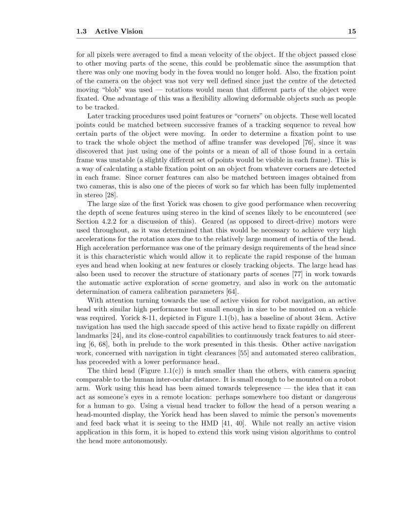
(a) (b) (c)
Figure 1.1: The Yorick series of active robot heads: (a) the original model used in surveil-lance, (b) Yorick 8-11 which is mounted on a vehicle and used for navigation, and (c)Yorick 55C which is small enough to be mounted on a robot arm and used in telepresenceapplications.
The Oxford Active Vision Project
Active vision research in Oxford has taken a mechatronic approach to providing the di-rectability of visual attention required by the paradigm. Early work [20] made use ofcameras mounted on robot arms, but it soon became clear that more specialised hardwarewas required to produce the high performance camera motions required by useful visionalgorithms, and this led to the construction on the Yorick series of active stereo heads (seeFigure 1.1). Designed by Paul Sharkey, there are currently three, each aimed at a certainapplication and differing primarily in size, but generically similar in their layout — all havetwo cameras and four axes of rotation (as in Figure 2.5).
The first Yorick [84] is a long-baseline model (about 65cm inter-ocular spacing) designedto be used for the dynamic surveillance of scenes. In surveillance, a robot observer mustbe able to detect, switch attention to and follow a moving target in a scene. By splittingimages obtained from an active camera into a low resolution periphery and a high resolutioncentral area or fovea, this can be achieved in a way which is potentially similar to how animaland human vision systems operate: any motion in the scene can be detected by measuringoptical flow in the coarse outer region, and then this information can be used to fire asaccade or rapid redirection of gaze direction so that the camera is facing directly towardsthe object of interest [67]. The saccades are programmed so that when the camera arrives ata position to look directly at the moving object, it is also moving at the estimated angularvelocity necessary to follow the object if it continues to move at the same speed. This makesit fairly simple to initiate some kind of tracking of the motion since the head will follow itfor a short while anyway if the acceleration of the object is not too large [11].
Tracking of objects has been performed in two ways. The aim has been to keep thehead moving such that the object of interest is continuously in the central foveal region ofthe image. The high definition of this area provides the detail necessary to detect smalldeviations from perfect alignment when corrections are needed. Initially, optical flow meth-ods were used in the fovea to successfully track objects over extended periods. While thisworked well, the very general nature of the method meant that it could break down — anymotion in the fovea was simply grouped together and the average of the optical flow vectors
1.3 Active Vision 15
for all pixels were averaged to find a mean velocity of the object. If the object passed closeto other moving parts of the scene, this could be problematic since the assumption thatthere was only one moving body in the fovea would no longer hold. Also, the fixation pointof the camera on the object was not very well defined since just the centre of the detectedmoving “blob” was used — rotations would mean that different parts of the object werefixated. One advantage of this was a flexibility allowing deformable objects such as peopleto be tracked.
Later tracking procedures used point features or “corners” on objects. These well locatedpoints could be matched between successive frames of a tracking sequence to reveal howcertain parts of the object were moving. In order to determine a fixation point to useto track the whole object the method of affine transfer was developed [76], since it wasdiscovered that just using one of the points or a mean of all of those found in a certainframe was unstable (a slightly different set of points would be visible in each frame). This isa way of calculating a stable fixation point on an object from whatever corners are detectedin each frame. Since corner features can also be matched between images obtained fromtwo cameras, this is also one of the pieces of work so far which has been fully implementedin stereo [28].
The large size of the first Yorick was chosen to give good performance when recoveringthe depth of scene features using stereo in the kind of scenes likely to be encountered (seeSection 4.2.2 for a discussion of this). Geared (as opposed to direct-drive) motors wereused throughout, as it was determined that this would be necessary to achieve very highaccelerations for the rotation axes due to the relatively large moment of inertia of the head.High acceleration performance was one of the primary design requirements of the head sinceit is this characteristic which would allow it to replicate the rapid response of the humaneyes and head when looking at new features or closely tracking objects. The large head hasalso been used to recover the structure of stationary parts of scenes [77] in work towardsthe automatic active exploration of scene geometry, and also in work on the automaticdetermination of camera calibration parameters [64].
With attention turning towards the use of active vision for robot navigation, an activehead with similar high performance but small enough in size to be mounted on a vehiclewas required. Yorick 8-11, depicted in Figure 1.1(b), has a baseline of about 34cm. Activenavigation has used the high saccade speed of this active head to fixate rapidly on differentlandmarks [24], and its close-control capabilities to continuously track features to aid steer-ing [6, 68], both in prelude to the work presented in this thesis. Other active navigationwork, concerned with navigation in tight clearances [55] and automated stereo calibration,has proceeded with a lower performance head.
The third head (Figure 1.1(c)) is much smaller than the others, with camera spacingcomparable to the human inter-ocular distance. It is small enough to be mounted on a robotarm. Work using this head has been aimed towards telepresence — the idea that it canact as someone’s eyes in a remote location: perhaps somewhere too distant or dangerousfor a human to go. Using a visual head tracker to follow the head of a person wearing ahead-mounted display, the Yorick head has been slaved to mimic the person’s movementsand feed back what it is seeing to the HMD [41, 40]. While not really an active visionapplication in this form, it is hoped to extend this work using vision algorithms to controlthe head more autonomously.

1.4 This Thesis: Navigation Using Active Vision 16
1.4 This Thesis: Navigation Using Active Vision
There have so far only been limited efforts to apply active vision to navigation, perhapslargely because of the complexity of building mobile robots with active heads, which onlya few laboratories are in a position to do.
1.4.1 Some Previous Work in Active Visual Navigation
Li [55] built on the work of Du [26], in using an active head to detect obstacles on the groundplane in front of a mobile robot, and also performing some active tracking of features with aview to obstacle avoidance. However, only limited results were presented, and in particularthe robot did not manoeuvre in response to the tracking information, and no attempt wasmade to link the obstacle-detection and obstacle-avoidance modules.
Beardsley et al. [6] used precisely controlled motions of an active head to determine theaffine structure of a dense point set of features in front of a robot, and then showed thatit was possible to initiate obstacle avoidance behaviours based on the limits of free-spaceregions detected. This work was impressive, particularly as it operated without needingknowledge of camera calibrations. It implemented in short demonstrations which workedwell, but consideration was not given to the long-term goals of navigation and how theactive head could be used in many aspects.
At NASA, Huber and Kortenkamp [42, 43] implemented a behaviour-based active visionapproach which enabled a robot to track and follow a moving target (usually a person).Correlation-based tracking was triggered after a period of active searching for movement,and extra vision modules helped the tracking to be stable. The system was not truly anactive vision navigation system, however, since sonar sensors were used for obstacle detectionand path planning.
1.4.2 A Unified Approach to Navigation with Active Vision
Active cameras potentially provide a navigating vehicle with the ability to fixate and trackfeatures over extended periods of time, and wide fields of view. While it is relativelystraightforward to apply fixating vision to tactical, short-term navigation tasks such asservoing around obstacles where the fixation point does not change [68], the idea of usingserial fixation on a succession of features to provide information for strategic navigation ismore involved. However, active vision is seemingly well-suited to this task: the ability tomeasure features over such a wide range means that the same ones can be used as a robotmakes a wide range of movements. This has advantages for map-building and localisationover the use of passive cameras with a narrow field of view.
The core work of this thesis concerns the problem of simultaneous localisation andmap-building for a robot with a stereo active head (Chapter 5), operating in an unknownenvironment and using point features in the world as visual landmarks (Chapter 4). Im-portance has been attached to producing maps which are useful for extended periods ofnavigation. As discussed in Section 1.2, many map-building methods fail on extended runsbecause they do not have the ability to recognise previously visited areas as such and ad-just their maps accordingly. With active cameras, the wide field of view means that wereally can expect to re-detect features found a long time ago, even if the area is not passedthrough along the original trajectory. Maintaining a large, consistent map requires detailed

1.4 This Thesis: Navigation Using Active Vision 17
information to be stored and updated about the estimates of all the features and their rela-tionships. This information is computationally expensive to maintain, but a sparse map oflandmark features can be handled successfully. In Section 6.2, a method is presented whichdramatically increases the efficiency of updates in the case that repeated measurements aremade of a single feature. This permits continuous real-time tracking of features to occurirrespective of the total map size.
The selective approach of active sensing means that a strategy must be developed forserially fixating on different features. This strategy is based on decisions about which mea-surements will provide the best information for maintaining map integrity, and is presentedin Section 6.3. When combined with criteria for automatic map maintenance in Chap-ter 7 (deciding when to add or delete features), a fully automatic map-building system isachieved.
Active sensing, when applied to navigation, could mean more than just selectively ap-plying the sensors available: the path to be followed by the robot could be altered in sucha way as to affect the measurements collected. This approach is used by Blake et al. [9],where a camera mounted on a robot arm makes exploratory motions to determine the oc-cluding contours of curved obstacles before moving in safe paths around them. Whaite andFerrie [100] move an active camera in such a way as to maximise the information gainedfrom a new viewpoint when determining the shape of an unknown object. In this thesis, itis assumed that the overall control of the robot’s motion comes from a higher-level process,such as human commands, or behaviours pulling it to explore or reach certain targets. Thenavigation capabilities sought should act as a “server” to these processes, supporting themby providing the necessary localisation information.
We will discuss in detail in Chapters 5 and 7 the tasks that an autonomous robot shouldbe able to perform. In most applications, there will be at least some prior informationor commands governing the required motion and we will look at how this informationcan be incorporated with map-building techniques designed for unknown environments.We will make the distinction between position-based navigation, and so-called context-based navigation, where the robot manoeuvres with respect to locally observed parts ofthe surroundings. A simple steering law is used to direct the robot sequentially aroundobstacles or through waypoints on a planned trajectory.
Throughout the thesis, a variety of experiments will be presented which test the ca-pabilities developed in a realistic environment and make extensive comparisons betweenestimated quantities and ground-truth. The system has been fully implemented on a realrobot, incorporating such capabilities as continuous fixated feature tracking and dynamicsteering control, and we will discuss system details as well as the mathematical modellingof the robot system necessary for accurate performance.
Some work using sonar rather than vision, but with an active approach which has per-haps most in common with this thesis was by Manyika [57]. Although sonar presents a differ-ent set of problems to vision, especially in terms of the more difficult feature-correspondenceissues which must be addressed, the use of tracking sensors to selectively make continuousmeasurements of features is closely related. He was concerned with sensor management:applying the available resources to the best benefit. However, the robot in Manyika’s workoperated in known environments, recognising features from a prior map, greatly simplifyingthe filtering algorithm used.
2The Robot System
The aim of this thesis, novel research into robot navigation using active vision, has de-manded an experimental system with the capability to support the modes of operationproposed. Since the aim of this thesis has been vision and navigation research rather thanrobot design, efforts have been made to keep the system simple, general (in the sense thatapart from the unique active head, widely available and generally functional componentshave been preferred over specialised ones), and easy to manage. This characterises therecent move away from highly specialised and expensive hardware in computer vision androbotics applications, and more generally in the world of computing where the same com-puter hardware is now commonly used in laboratories, offices and homes.
2.1 System Requirements
The system requirements can be broken down into four main areas:
• Robot vehicle platform
• Vision acquisition and processing
• Active control of vision
• System coordination and processing
The approach to navigation in this thesis is suited to centralised control of the systemcomponents. From visual data acquired from the robot’s cameras, decisions must be madeabout the future behaviour of the cameras and the motion of the vehicle. Signals must thenbe relayed back to the active camera platform and vehicle. Their motion will affect the

2.1 System Requirements 19
Figure 2.1: The robot used in this thesis comprises an active binocular head, equipped withtwo video cameras, mounted on a three-wheeled vehicle.
Head Commands
Images
Processing
Vehicle Commands
Cameras
SceneActive Head
Vehicle
VisualData
Figure 2.2: The basic flow of information around the robot system.
next batch of visual data acquired. The essential flow of information around the system isdepicted in block form in Figure 2.2.
2.1.1 System Composition
There have been two stages in putting the system together in its current form. The first,which was in place when the work in this thesis was started, made use of the hardwareavailable at the time from other projects to make a working, but convoluted system. Inparticular, the setup included a Sun Sparc 2 workstation acting as host and an i486 PChosting the head controller and transputers communicating with the vehicle. Image ac-quisition was performed by external Datacube MaxVideo boards, and most of the imageprocessing was carried out on a network of transputers, again separately boxed from therest of the system.
2.2 A PC/Linux Robot Vision System 20
Head Powerand Encoder
Cables
Video Cables
RS 422Link
VehicleBatteries
VehicleController
Video Signals
VehicleCommands
Head Odometry
Head MotorCurrents
Head Demands
Head AmplifiersPentium PC
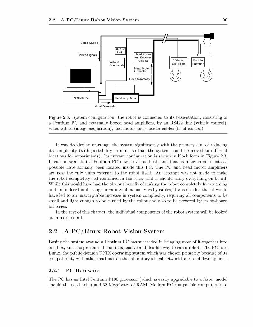
Figure 2.3: System configuration: the robot is connected to its base-station, consisting ofa Pentium PC and externally boxed head amplifiers, by an RS422 link (vehicle control),video cables (image acquisition), and motor and encoder cables (head control).
It was decided to rearrange the system significantly with the primary aim of reducingits complexity (with portability in mind so that the system could be moved to differentlocations for experiments). Its current configuration is shown in block form in Figure 2.3.It can be seen that a Pentium PC now serves as host, and that as many components aspossible have actually been located inside this PC. The PC and head motor amplifiersare now the only units external to the robot itself. An attempt was not made to makethe robot completely self-contained in the sense that it should carry everything on-board.While this would have had the obvious benefit of making the robot completely free-roamingand unhindered in its range or variety of manoeuvres by cables, it was decided that it wouldhave led to an unacceptable increase in system complexity, requiring all components to besmall and light enough to be carried by the robot and also to be powered by its on-boardbatteries.
In the rest of this chapter, the individual components of the robot system will be lookedat in more detail.
2.2 A PC/Linux Robot Vision System
Basing the system around a Pentium PC has succeeded in bringing most of it together intoone box, and has proven to be an inexpensive and flexible way to run a robot. The PC usesLinux, the public domain UNIX operating system which was chosen primarily because of itscompatibility with other machines on the laboratory’s local network for ease of development.
2.2.1 PC Hardware
The PC has an Intel Pentium P100 processor (which is easily upgradable to a faster modelshould the need arise) and 32 Megabytes of RAM. Modern PC-compatible computers rep-
2.2 A PC/Linux Robot Vision System 21
PMAC Controller Card
PMAC Dual−Ported RAM
B008 Transputer Card
Matrox Meteor (Video Capture)
Matrox Millenium (Video Display)
Ethernet Card
ISA Slots
PCI Slots
Ribbon Cable to Head Amplifier
Network Connection
Coax to Video Cameras
To Monitor
RS422 Link to Vehicle Controller
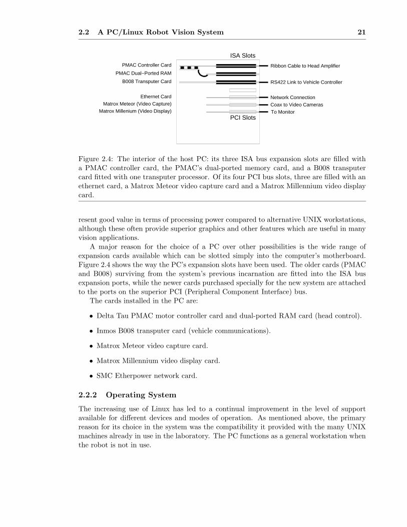
Figure 2.4: The interior of the host PC: its three ISA bus expansion slots are filled witha PMAC controller card, the PMAC’s dual-ported memory card, and a B008 transputercard fitted with one transputer processor. Of its four PCI bus slots, three are filled with anethernet card, a Matrox Meteor video capture card and a Matrox Millennium video displaycard.
resent good value in terms of processing power compared to alternative UNIX workstations,although these often provide superior graphics and other features which are useful in manyvision applications.
A major reason for the choice of a PC over other possibilities is the wide range ofexpansion cards available which can be slotted simply into the computer’s motherboard.Figure 2.4 shows the way the PC’s expansion slots have been used. The older cards (PMACand B008) surviving from the system’s previous incarnation are fitted into the ISA busexpansion ports, while the newer cards purchased specially for the new system are attachedto the ports on the superior PCI (Peripheral Component Interface) bus.
The cards installed in the PC are:
• Delta Tau PMAC motor controller card and dual-ported RAM card (head control).
• Inmos B008 transputer card (vehicle communications).
• Matrox Meteor video capture card.
• Matrox Millennium video display card.
• SMC Etherpower network card.
2.2.2 Operating System
The increasing use of Linux has led to a continual improvement in the level of supportavailable for different devices and modes of operation. As mentioned above, the primaryreason for its choice in the system was the compatibility it provided with the many UNIXmachines already in use in the laboratory. The PC functions as a general workstation whenthe robot is not in use.

2.3 The Active Head: Yorick 22
Pan Axis
ElevationAxis
LeftVergence Axis
RightVergence Axis
Figure 2.5: Yorick 8-11 has pan, elevation and twin vergence axes of movement.
Linux is an operating system which lies entirely in the public domain, meaning thatwhile it comes with no guarantees or software support, the user is free to use it for anypurpose, and the source code is available so that custom modifications can be made.
Two disadvantages of using Linux were:
• At the time of the reconfiguration of the system, Linux device drivers were not avail-able for either the Matrox Meteor video capture card or the PMAC motor controllercard. It was necessary to confer with others wanting to use these cards under Linuxand to play a part in successfully developing the drivers.
• Linux is not a “real-time” operating system in the sense that the timing of programscan be guaranteed; they may be interrupted to perform other system tasks. In prac-tice, this did not prove to be a large problem. The necessary timing signals for thecoordination of the composite robot system were obtained from component sourcessuch as the video capture card or the vehicle controller, and allowances made for apotential loss of processing time due a short interruption.
A Linux system can be easily run in “single machine” mode, so that the computer canbe disconnected from its local network. This was important so that the system could beportable.
2.3 The Active Head: Yorick
The active camera platform used on the robot, Yorick 8-11, is one of the series of headsbuilt in Oxford already described in Chapter 1.
The purpose of the head is to enable the two video cameras it carries to be directed asrequired by a robot performing navigation tasks. The “common elevation” head geometry,with four axes of movement as shown in Figure 2.5, means that the two cameras movetogether as the pan and elevation angles are changed, and can be converged (symmetrically
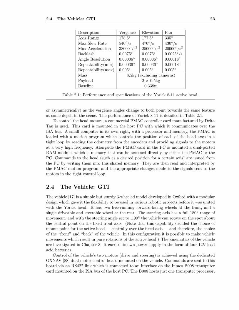
2.4 The Vehicle: GTI 23
Description Vergence Elevation Pan
Axis Range 178.5◦ 177.5◦ 335◦
Max Slew Rate 540◦/s 470◦/s 430◦/sMax Acceleration 38000◦/s2 25000◦/s2 20000◦/s2
Backlash 0.0075◦ 0.0075◦ 0.0025◦/sAngle Resolution 0.00036◦ 0.00036◦ 0.00018◦
Repeatability(min) 0.00036◦ 0.00036◦ 0.00018◦
Repeatability(max) 0.005◦ 0.005◦ 0.005◦
Mass 8.5kg (excluding cameras)Payload 2 × 0.5kgBaseline 0.338m
Table 2.1: Performance and specifications of the Yorick 8-11 active head.
or asymmetrically) as the vergence angles change to both point towards the same featureat some depth in the scene. The performance of Yorick 8-11 is detailed in Table 2.1.
To control the head motors, a commercial PMAC controller card manufactured by DeltaTau is used. This card is mounted in the host PC with which it communicates over theISA bus. A small computer in its own right, with a processor and memory, the PMAC isloaded with a motion program which controls the position of each of the head axes in atight loop by reading the odometry from the encoders and providing signals to the motorsat a very high frequency. Alongside the PMAC card in the PC is mounted a dual-portedRAM module, which is memory that can be accessed directly by either the PMAC or thePC. Commands to the head (such as a desired position for a certain axis) are issued fromthe PC by writing them into this shared memory. They are then read and interpreted bythe PMAC motion program, and the appropriate changes made to the signals sent to themotors in the tight control loop.
2.4 The Vehicle: GTI
The vehicle [17] is a simple but sturdy 3-wheeled model developed in Oxford with a modulardesign which gave it the flexibility to be used in various robotic projects before it was unitedwith the Yorick head. It has two free-running forward-facing wheels at the front, and asingle driveable and steerable wheel at the rear. The steering axis has a full 180◦ range ofmovement, and with the steering angle set to ±90◦ the vehicle can rotate on the spot aboutthe central point on the fixed front axis. (Note that this capability decided the choice ofmount-point for the active head — centrally over the fixed axis — and therefore, the choiceof the “front” and “back” of the vehicle. In this configuration it is possible to make vehiclemovements which result in pure rotations of the active head.) The kinematics of the vehicleare investigated in Chapter 3. It carries its own power supply in the form of four 12V leadacid batteries.
Control of the vehicle’s two motors (drive and steering) is achieved using the dedicatedOXNAV [88] dual motor control board mounted on the vehicle. Commands are sent to thisboard via an RS422 link which is connected to an interface on the Inmos B008 transputercard mounted on the ISA bus of the host PC. The B008 hosts just one transputer processor,
2.5 Image Capture 24
whose job is to receive motion commands from the PC and translate them into commandsto send to the OXNAV board along the RS422 link.
The control performance of the vehicle is relatively low (certainly compared to the activehead), in the sense that a command for a certain motion can produce a result that differsfrom the command by an unpredictable amount within a reasonably large range. This isdue mainly to slippage between the wheels and the floor, but also to the deliberately fairlyapproximate calibration of the vehicle. However, this is not a problem with regard to thework presented in this thesis, since it is exactly these kind of errors in motion estimationwhose effect it is hoped to determine and correct by visual localisation and navigation.
The peak forward velocity of the vehicle is of the order of 20cms−1.
2.5 Image Capture
The cameras used on Yorick 8-11 are compact CCD devices producing standard monochromePAL output at a frequency of 50Hz. In the robot system, the cameras are powered fromthe vehicle’s 12V batteries.
The Matrox Meteor image capture card is able to grab PAL frames at the full interlacedresolution of 768× 576 pixels and make them available to the host PC over the PCI bus atfield rate. The Meteor is designed for colour image acquisition from either a composite videosource or separate synchronous red, green and blue (RGB) inputs. In the robot system,colour is not required, but there are two monochrome cameras. Simultaneous capture fromthese was achieved with just one Meteor by connecting the cameras to two of the RGBchannels as if their signals were just different colour fields from a single camera. TheMeteor composites these signals into a single mixed image where bytes from the left andright camera images alternate in a regular pattern; it is an easy task to separate out theimages for processing and displaying.
For speed, in the final system images are subsampled down to 192 × 144 pixels beforeprocessing.
2.6 Software
The approach to software in the system has been simplified by its centralised PC-basedconstruction, which minimised worries about communication between different components.As mentioned earlier, commands to the robot and active head are communicated via theirLinux drivers. Images from the framegrabber are read with calls to its driver. A centralprogram running on the PC is therefore able to control all parts of the system. All imageand navigation processing are performed by the Pentium processor.
The main program controlling the system was written in C++. An important require-ment during the development of the system was the capability to test ideas and algorithmsin simulation before full robot implementation. With this in mind, the main program wasdesigned with dual simulation / robot modes of operation as a fundamental feature, andeasy switching between the two while keeping as much code as possible in common waspermitted. The object-oriented nature of C++ made this easy to achieve. Interchangeable“Robot” and “Simulation” classes were created which had the same interface: a call to amember function of the Robot class would cause an actual result, such as a robot motion,

2.7 Working in Real Time 25
while the equivalent call to the Simulation class would cause the simulation of the robotand world to change accordingly. A choice at compile-time indicates which mode the pro-gram will operate in. The main classes of the program which are common to Simulationand Robot modes are “Scene”, which contains and maintains estimates of the positions ofthe robot and features in world, and “Kalman”, which contains functions to perform filterupdates. These classes should make it straightforward to transplant the map-building andlocalisation algorithm of this thesis to a different robot.
For display purposes and the fast processing of matrices, routines from the Horatio [62]vision libraries were used. The need for fast operation dissuaded the use of a dedicatedC++ library such as the Image Understanding Environment since at the time of writingwork on real-time sections is still in progress.
2.7 Working in Real Time
When moving and tracking features simultaneously, the system executes a loop at a fre-quency of 5Hz, at each step of which a motion prediction is made, the head moves, imagesare acquired and displayed, image processing occurs and updates to all the estimated quan-tities take place. Implementation details will be discussed further in Chapters 5 and 6.However, we will quickly note that the main factor limiting speed of operation was the pro-cessing time needed to perform image processing on the stereo images. Vehicle odometry isused to provide the trigger for the loop timing: a new image is acquired when the vehiclehas reached a certain position according to readings from its wheel encoder. In this sense,the update frequency is linked to distances travelled by the vehicle, and so 5Hz is only anapproximate value calculated from the vehicle calibration. The program has the ability toadjust the rate of measurements automatically in reponse to time over-runs in the process-ing stages: as will be explained later, this can happen in normal circumstances when thereis a large amount of image processing to do, but another possibility is lost processing dueto an interruption from another Linux process.
2.8 Calibration
Most aspects of the robot system were used in a calibrated configuration in the work in thisthesis. However, the calibrations used were approximate apart from with the active head,whose geometry is very well known.
• Cameras: The focal lengths were determined to two significant figures with a simplemeasurement of the image size of a known object at a known distance. The principalpoints used were usually the camera image centres, which have been shown in previousaccurate calibrations of the cameras to be close to the true locations. Measurementsmade by the active head at fixation (see Section 4.2) are much more sensitive to errorsin the principal points than the focal lengths. The same calibration values were usedfor both of the robot’s cameras (see Section 3.2 for details of the pinhole cameramodel).
Automated camera calibration is now an important area of computer vision research,and self-calibration of stereo rigs has also been tackled [25, 55]. However, it is felt

2.8 Calibration 26
that this work is somewhat adjacent to the work in this thesis, where the emphasis ison using a calibrated active camera system effectively for navigation.
• Head: Section 3.3 describes the mathematical model used of the active head. Theconstant dimensions of the head encoded in the constants H, I, p, c and n are wellknown from the head design or measurements. Yorick 8-11 does not have well defined“end stops” on its axes, or another automatic way to repeatably find their zero loca-tions, so this was normally achieved by moving them by hand each time the systemwas started. It is estimated that a zero accuracy of around 1◦ could easily be achievedin this way. Previous work with Yorick [75] demonstrated an automatic vision-basedmethod for centering the elevation and vergence axes which achieved accuracy of thisorder.
• Vehicle: For the vehicle motion model (Section 3.4), it was necessary to know thescaling between control inputs and movements of the steering axis and driving wheel.The steering axis was well calibrated as standard in the OxNav controller, so thata steering demand of 10◦ reliably represented an actual 10◦ movement. The drivingwheel scaling was calibrated by hand to two significant figures in a measured runwhere the odometry count was noted. This is a quantity which could actually beestimated by the robot during its navigation with a change to the map-building andlocalisation algorithm, since there need only be one quantity determining overall scalein the system, and it is sensible for this to come from the head measurements. Thiswould eliminate a potential source of bias in estimations if calibration is incorrect.As the system stands, the drive scaling is used as well, although in the estimationprocesses is is given less weight than the head measurements since it is assumed notto be well known.

3Robot Models and Notation
This chapter describes the mathematical models which have been constructed of the cam-eras, active head and vehicle which make up the robot used in this research.
It has been considered important to use models which are realistic when reasonablypossible. In particular, there is no reason to make approximations with models when thetrue situation is not difficult to analyse and a large gain is not made by approximating. Acase where an approximation can be useful is where it allows some previously developedtheory to be applied easily, and we will give an example of this in Section 4.3. However, itis felt that simplifications are sometimes used too quickly in situations where they are notnecessary.
3.1 Notation
The notation used in this thesis broadly follows conventions in computer vision, but wewill describe the exact meanings of certain representations here, particularly with regard tovectors.
3.1.1 Vectors
When we write a vector like a in bold type but with no superscript, we mean a physicalvector in 3D space independent of any frames of reference we may have introduced. Withvectors of this type we can write vector equations such as
a = b + c
without specifying a coordinate system. This equation simply represents the geometricarrangement in Figure 3.1.

3.1 Notation 28
a
b
c
Figure 3.1: The vector sum a = b + c.
Subscripts are sometimes used to differentiate between different physical vectors, thoughones with a similar role — for instance cL and cR on the left and right sides of the activehead in Section 3.3.
3.1.2 Reference Frames
A frame of reference, denoted in this thesis by a capital letter such as F or a capital letterand a number such as C0, is an imaginary alignment of a set of xyz axes in Euclidean 3Dspace. When vectors are being considered, it is only the orientation of this set of axes whichis important, not the position of its origin, since vectors are differences between positions,rather than absolute positions in a given reference frame.
Superscripts are used to relate vectors to reference frames. By the notation aF we meanthe mathematical 3-component vector whose components constitute the spatial vector a inthe reference frame F :
aF =
aFx
aFy
aFz
.
Hence, for example, given the spatial equation a = b + c, we can deduce a componentequation aF = bF + cF in a particular frame of interest.
It will invariably be possible to represent all physical quantities of interest as vectors.For instance, with a point in space defined as an origin, such as the optic centre of a camera,locations of features in the scene relative to this point can be represented by the vectorsfrom the origin to the features (their position vectors). Sometimes, though, in situationslike this we will talk about the absolute positions of features in a reference frame centredat the origin — meaning that the location of the reference axes is specified as well as theirorientation. This nomenclature can clarify situations where many vectors emanate from thesame origin point. We will, however, return to a vector-based representation and referenceframes specified only by their orientations when transformations are to be considered, asthis method trivialises their application.
3.1.3 Rotations
We will frequently need to transform a vector from one frame to another — that is to say,given the components of a vector in one frame of reference, calculate its components inanother. This transformation will take the form of a rotation matrix. We define RFG tobe the rotation matrix which produces the components of a vector in frame F from itscomponents in frame G:
aF = RFGaG .

3.2 Camera Model 29
zx
y
u
v (x , y , f)c c
(u , v )0 0
h
f
Optic Axis
Camera Image PlaneOptic Centre O
Scene Feature P
Image Point p
Camera Frame Fp
Figure 3.2: The pinhole camera model with focal length f and principal point (u0, v0).
Note how the two frame superscripts of R are seen to be “adjacent” to their respectivevectors in the equation.
The reverse transformation is easily formulated, since a rotation, as an orthogonal ma-trix, has an inverse equal to its transpose:
aG = RGFaF ,
whereRGF = (RFG)> .
These rotation transformations should not be thought of as any kind of movement ofthe vector under consideration in the real world — the spatial vector a is a fixed entityrepresenting a physical quantity. We are simply dealing with the representation of thisvector in imagined frames of reference placed in the world.
3.2 Camera Model
Figure 3.2 shows the customary pinhole model of a CCD video camera which was used inthis work. For ease of representation, the camera’s image plane is shown in front of theoptic centre instead of in its true position behind. A vector h from the optic centre O to afeature P in the scene intersects the image plane at position p, and this is where the featurewill be imaged.
A camera-centred coordinate frame F is defined with origin at O, its z axis aligned withthe camera’s optic axis, and its x and z axes parallel to the image plane in the horizontaland vertical directions respectively. In this frame, h has components:
hF =
hFx
hFy
hFz
.
The position vector p of the image point p is parallel to h, but shorter by a factor f/hFz .
In frame F , the components of p are:
pF =
xc
yc
f
=
f
hFz
hF .

3.2 Camera Model 30
xc and yc are the coordinates of p on the image plane. Now the real image plane is madeup of pixels which are spaced at ku pixels m−1 and kv pixels m−1 in the horizontal andvertical directions respectively. (u0, v0) is the pixel position of the point where the opticaxis crosses the plane. Hence the pixel coordinates of the point (xc, yc, f) on the plane aregiven by
u = u0 − kuxc
andv = v0 − kvyc.
We can write these equations in the form:
uv1
=
−ku 0 u0/f0 −kv v0/f0 0 1/f
xc
yc
f
,
or
uv1
=
−ku 0 u0/f0 −kv v0/f0 0 1/f
pF .
Vector pF is parallel to hF . We can therefore write:
uv1
∝
−fku 0 u0
0 −fkv v0
0 0 1
hF ,
where we have multiplied through by the constant f to obtain the familiar form of theperspective projection equation:
uv1
∝ ChF , (3.1)
where
C =
−fku 0 u0
0 −fkv v0
0 0 1
is the camera calibration matrix, encoding information about the camera’s intrinsic param-eters f , ku, kv, u0 and v0. This equation relates the 3D location of a scene point in the
camera reference frame to the homogeneous vector(
u v 1)>
describing the pixel loca-
tion of its image. The homogeneous notation is used because it makes it easy to invert theequation to obtain the inverse relation:
hF ∝ C−1
uv1
, (3.2)
with
C−1 =
−1fku
0 u0
fku
0 −1fkv
v0
fkv
0 0 1
.

3.3 Active Head Model 31
Head Centre
Scene Feature
H
cL
nL
pL
hL
hR
hG
Figure 3.3: A vector model of the Yorick active head. H goes vertically from the groundplane to the head centre — the point where the pan axis meets the horizontal plane con-taining the elevation axis. pL, cL and nL combine to represent the offset from the headcentre to the left camera’s optic centre, with pR, cR and nR (not shown) doing the same forthe right camera. hL and hR are vectors from the optic centres to a feature in the scene.hG is a calculated vector from the head centre to the feature.
This allows the vector location up to a scale factor of a scene feature to be calculated fromits image position (assuming knowledge of C) — meaning that the point’s 3D location isknown to be somewhere along the line defined by all possible lengths of h.
3.3 Active Head Model
Figure 3.3 shows the vector model used to represent the active head. The geometry of thehead is complicated by the fact that there are small offsets between the axes of rotation, andcare has been taken to represent the effect of these. The purpose of the model is to enablethe calculation of forward and backward projections through the head system; specifically:
1. The image coordinates at which a known 3D point in the scene will be found in theleft and right cameras.
2. The head joint angles necessary to fixate a known 3D point.
3. The 3D position of a point whose image coordinates are known.
3.3.1 The Head Centre
A point on the active head is defined which does not move when the head rotates and whichis therefore fixed relative to the vehicle which carries the head. This point is called the“head centre”, and is the intersection of the vertical pan axis with the horizontal planewhich always contains the elevation axis. The head centre is a reference point between thetwo cameras which can be used as the origin of measurements from a hypothetical cyclopeansensor. The vector hG will represent the displacement from the head centre to a feature ofinterest in the scene.

3.3 Active Head Model 32
y
xz
Vehicle Frame C0
Elevated Frame C2
Panned Frame C1
Verged Frames L, R
C0
C1
C2
C0
C1
C2
C0
C1
C2
y
x
z
z
y
x
α
e
L
L
Ly
x
zγL
R
R
R
z
x
y
γR
Figure 3.4: The frames of reference used in the head model.
The head’s encoders provide continuous and accurate information on the angles of itsrotation axes. Knowledge of these angles means that is is always possible to calculate thelocation and orientation of the two cameras relative to the head centre.
3.3.2 Reference Frames
Referring back to Figure 2.5 showing the Yorick’s rotation axes, and to Figure 3.4, weintroduce the reference frames used when describing the head. When the head angles areall zero, both cameras will point directly forwards and all of these frames will be aligned withC0. The reason for introducing these frames is that each of the vectors in the head modelin Figure 3.3 can be represented in a simple way in one of them, being either constant inthe case of the internal head vectors H, pL, pR, cL, cR, nL and nR, or in the representationin which they will be useful in the case of the “end result” vectors hL, hR and hG.
• C0 is the vehicle frame which is fixed relative to the vehicle. Its z axis lies in theforward direction, with the y-axis pointing up and the x axis to the left. In thisframe:
HC0 =
0H0
, hC0
G =
hC0Gx
hC0Gy
hC0Gz
.
• C1 is the panned frame which is fixed relative to the parts of the head that movewhen the pan angle changes. Its y axis stays vertical, and its x and z axes remain inthe horizontal plane, with its x axis always parallel to the head’s elevation axis. It ishorizontally rotated with respect to C0 by the pan angle α. In this frame:
pC1L =
I/20p
, pC1
R =
−I/20p
.

3.3 Active Head Model 33
• C2 is the elevated frame which is fixed relative to the parts of the head that movewhen the elevation changes. Its y axis stays parallel to the two vergence axes, and itsx axis is aligned with the elevation axis. It is vertically rotated with respect to C1 byelevation angle e. In this frame:
cC2L =
0c0
, cC2
R =
0c0
.
• L and R are the left and right camera frames respectively, fixed relative to the twocameras. Their z axes are aligned with the camera optic axes, and their x and y axeslie parallel to their image planes. These frames are rotated with respect to C2 byvergence angles γL and γR respectively. In these frames:
nLL =
00n
, hL
L =
hLLx
hLLy
hLLz
,
nRR =
00n
, hR
R =
hRRx
hRRy
hRRz
.
H, I, p, c, and n are scalar distances representing the dimensions of the head:
• H is the vertical distance of the head centre above the ground plane.
• I the is horizontal distance between the vergence axes (the inter-ocular distance be-tween the camera optic centres if both cameras are facing forwards).
• p is the horizontal offset between the pan and elevation axes.
• c is the offset along either vergence axis between the intersections with the elevationaxis and the camera optic axis.
• n is the offset along either optic axis between the camera optic centre and the inter-section with the vergence axis.
The rotation matrices transforming between these reference frames have trivial formsdue to their simple relationships:
RC10 =
cos α 0 − sin α0 1 0
sin α 0 cos α
RC21 =
1 0 00 cos e − sin e0 sin e cos e
RLC2 =
cos γL 0 − sin γL
0 1 0sin γL 0 cos γL

3.3 Active Head Model 34
RRC2 =
cos γR 0 − sin γR
0 1 0sin γR 0 cos γR
3.3.3 Using the Model
With this framework in place, the expressions required from the model can easily be calcu-lated. Referring to Figure 3.3, we may form the two spatial vector equations:
hG = pL + cL + nL + hL , (3.3)
hG = pR + cR + nR + hR . (3.4)
Finding the Image Coordinates of a Known 3D Point
Consider first the case where hC0G , the location of a 3D point relative the the head centre in
the vehicle coordinate frame, is known, and we wish to calculate its image position in theleft and right cameras (assuming that it is in their fields of view): for the left camera, weform Equation 3.3 in the left camera coordinate frame L:
hLL = hL
G − pLL − cL
L − nLL .
Rephrasing this equation with transformations so that vectors can be used in their naturalreference frames:
hLL = R
LC0hC0G − R
LC1pC1L − R
LC2cC2L − nL
L ,
or, dividing the transformations into their known, simple, components:
hLL = R
LC2(RC21(RC10hC0G − pC1
L ) − cC2L ) − nL
L . (3.5)
For the right camera:
hRR = R
RC2(RC21(RC10hC0G − pC1
R ) − cC2R ) − nR
R . (3.6)
These are the equations in the form in which they will be used. They allow hLL and hR
R tobe found — these are the vectors from the left and right optic centres to the scene pointin the left and right camera coordinate frames respectively. From Equation 3.1 the point’simage coordinates can be determined:
uL
vL
1
∝ ChL
L ,
uR
vR
1
∝ ChR
R . (3.7)
Finding the Head Angles to Fixate a Known Point
We will frequently need to fixate a 3D point at a known location hC0G relative the the head
centre — that is, drive the active head so that both cameras point directly towards it. Tocalculate the head angles required, we must first decide how to deal with the redundancyintroduced by the head geometry: there are many sets of angles possible. We choose alwaysto use symmetric fixation: the vergence angles are required to be equal and opposite.
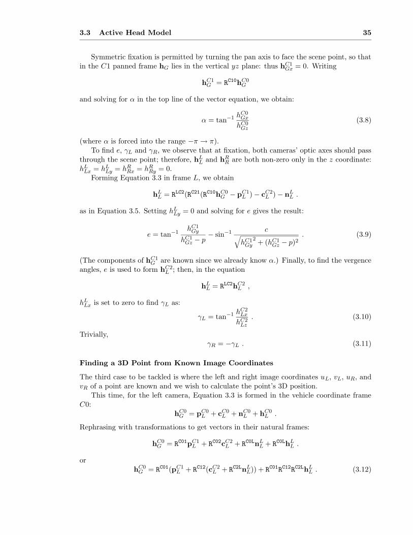
3.3 Active Head Model 35
Symmetric fixation is permitted by turning the pan axis to face the scene point, so thatin the C1 panned frame hG lies in the vertical yz plane: thus hC1
Gx = 0. Writing
hC1G = R
C10hC0G
and solving for α in the top line of the vector equation, we obtain:
α = tan−1 hC0Gx
hC0Gz
(3.8)
(where α is forced into the range −π → π).To find e, γL and γR, we observe that at fixation, both cameras’ optic axes should pass
through the scene point; therefore, hLL and hR
R are both non-zero only in the z coordinate:hL
Lx = hLLy = hR
Rx = hRRy = 0.
Forming Equation 3.3 in frame L, we obtain
hLL = R
LC2(RC21(RC10hC0G − pC1
L ) − cC2L ) − nL
L .
as in Equation 3.5. Setting hLLy = 0 and solving for e gives the result:
e = tan−1hC1
Gy
hC1Gz − p
− sin−1 c√
hC1Gy
2+ (hC1
Gz − p)2. (3.9)
(The components of hC1G are known since we already know α.) Finally, to find the vergence
angles, e is used to form hC2L ; then, in the equation
hLL = R
LC2hC2L ,
hLLx is set to zero to find γL as:
γL = tan−1 hC2Lx
hC2Lz
. (3.10)
Trivially,γR = −γL . (3.11)
Finding a 3D Point from Known Image Coordinates
The third case to be tackled is where the left and right image coordinates uL, vL, uR, andvR of a point are known and we wish to calculate the point’s 3D position.
This time, for the left camera, Equation 3.3 is formed in the vehicle coordinate frameC0:
hC0G = pC0
L + cC0L + nC0
L + hC0L .
Rephrasing with transformations to get vectors in their natural frames:
hC0G = R
C01pC1L + R
C02cC2L + R
C0LnLL + R
C0LhLL .
orhC0
G = RC01(pC1
L + RC12(cC2
L + RC2LnL
L)) + RC01
RC12
RC2LhL
L . (3.12)
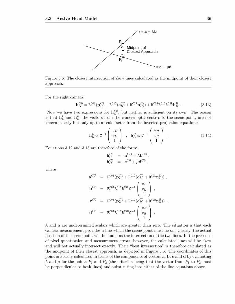
3.3 Active Head Model 36
r a b= + λ
r c d= + µ
Midpoint ofClosest Approach
P
P
1
2
Figure 3.5: The closest intersection of skew lines calculated as the midpoint of their closestapproach.
For the right camera:
hC0G = R
C01(pC1R + R
C12(cC2R + R
C2RnRR)) + R
C01RC12
RC2RhR
R . (3.13)
Now we have two expressions for hC0G , but neither is sufficient on its own. The reason
is that hLL and hR
R, the vectors from the camera optic centres to the scene point, are notknown exactly but only up to a scale factor from the inverted projection equations:
hLL ∝ C
−1
uL
vL
1
, hR
R ∝ C−1
uR
vR
1
. (3.14)
Equations 3.12 and 3.13 are therefore of the form:
hC0G = aCO + λbC0 ,
hC0G = cC0 + µdC0 ,
where
aCO = RC01(pC1
L + RC12(cC2
L + RC2LnL
L)) ,
bC0 = RC01
RC12
RC2L
C−1
uL
vL
1
,
cC0 = RC01(pC1
R + RC12(cC2
R + RC2RnR
R)) ,
dC0 = RC01
RC12
RC2R
C−1
uR
vR
1
.
λ and µ are undetermined scalars which are greater than zero. The situation is that eachcamera measurement provides a line which the scene point must lie on. Clearly, the actualposition of the scene point will be found as the intersection of the two lines. In the presenceof pixel quantisation and measurement errors, however, the calculated lines will be skewand will not actually intersect exactly. Their “best intersection” is therefore calculated asthe midpoint of their closest approach, as depicted in Figure 3.5. The coordinates of thispoint are easily calculated in terms of the components of vectors a, b, c and d by evaluatingλ and µ for the points P1 and P2 (the criterion being that the vector from P1 to P2 mustbe perpendicular to both lines) and substituting into either of the line equations above.

3.4 Vehicle Model 37
x
z
Robot at Starting Position (0, 0, 0)
Robot atLater Position (z, x, )
Fixed World Coordinate Frame
z
x
C0
C0
C0 Coordinate FrameCarried With Vehicle
φφ
Figure 3.6: The vehicle’s location in the world coordinate frame is specified with the coor-dinates (z, x, φ). The C0 coordinate frame is carried with the vehicle.
3.4 Vehicle Model
We have assumed that the robot vehicle moves on a perfect ground-plane at all times. Aworld coordinate frame W is defined such that its x and z axes lie in the ground plane, andits y axis points vertically upwards. The robot’s position on the ground is specified by thecoordinates (z, x, φ), where z and x are the world-frame coordinates of the head centre (itsposition in the y direction being constant), and φ is the robot’s orientation relative to theworld z axis.
As shown in Figure 3.6, at the start of its motion the vehicle’s location in the worldframe is defined to be z = 0, x = 0, φ = 0, and the world and vehicle frames are coincident(we will discuss this further in Chapter 5).
3.4.1 Moving the Robot
As described in the previous chapter, our robot vehicle has three wheels: two of these arefree-running but fixed to be forward-facing, and lie along the same axis at the front of thevehicle. The head centre lies vertically above this axis. The third wheel at the rear issteerable and also provides the drive.
With no transverse slipping of the wheels across the floor, setting a steering angle of sat the rear wheel means that points on the vehicle will travel in circular paths about thecentre of rotation at the intersection of the wheel axes. From Figure 3.7 we see that theradius of the path that the “head centre” moves in is
R = L/ tan(s) .
The radius of the path that the rear driving wheel moves in is
Rd = L/ sin(s) .
The control inputs to the vehicle which determine its motion are the steering angle s andthe velocity v at which the rear wheel is driven. Consider a period of time ∆t in which

3.4 Vehicle Model 38
L
Position(k+1)
Position(k)
Head Centre
d
K
s
R
R
s
Figure 3.7: With the angle of the vehicle’s single rear steering wheel set to s(k), the “headcentre”, lying centrally above the fixed axis of the front wheels, moves in a path of radiusR(k) = L/ tan(s(k)). L is the vehicle’s constant wheelbase.
both v and s are held at constant values: since the radius of the circular path along whichthe driving wheel moves is Rd, the angle in radians through which the vehicle moves alongits circular trajectory is
K = v∆t/Rd .
We can calculate the change in location of the head centre:
z(t + ∆t) = z(t) + R (cos φ(t) sin K + sin φ(t)(cos K − 1)) (3.15)
x(t + ∆t) = x(t) + R (sin φ(t) sin K + cos φ(t)(1 − cos K)) (3.16)
φ(t + ∆t) = φ(t) + K (3.17)
These are exact expressions and do not require ∆t to be small. They are equally valid forbackward vehicle motions if v has a negative value. Note that for the special case wheres = 0 (straight line motion) we must use a limiting form of these equations since R and Rd
become infinite:
z(t + ∆t) = z(t) + v∆t cosφ(t) (3.18)
x(t + ∆t) = x(t) + v∆t sin φ(t) (3.19)
φ(t + ∆t) = φ(t) (3.20)
3.4.2 Errors in Motion Estimates
Clearly, if we were able to rely precisely on these equations to calculate how the robot wasmoving after being sent control inputs v and s, it would not be necessary to use visionor other sensors to provide localisation information. The robot will, however, not moveexactly in the way predicted by the equations due to a number of possible factors: these

3.4 Vehicle Model 39
include slipping of the wheels and incorrect calibration of the vehicle controller. The resultwill be that although the expressions above will represent our best estimate of the vehicle’sposition, we must assign an uncertainty to this estimate.
The uncertainty is modelled as Gaussian variation in the effective control inputs v ands from the demanded values. In case of the steering angle s, the variation was given aconstant standard deviation σs of around 8◦, but with the velocity input v it was moreappropriate to assign a standard deviation which was proportional to the velocity demanditself — meaning that large motions are more uncertain than small ones. We used σv = σfv,with σf ≈ 0.15.
Naming the estimated position vector fv and the control vector u:
fv =
z(t + ∆t)x(t + ∆t)φ(t + ∆t)
, u =
(
vs
)
, (3.21)
we can calculate Q, the covariance matrix for fv, using the standard formula for transfer ofuncertainty at first order:
Q =∂fv∂u
U∂fv∂u
>
, (3.22)
where ∂fv∂u
is the Jacobian between fv and u, and U is the covariance matrix of u:
∂fv∂u
=
∂z(t+∆t)∂v
∂z(t+∆t)∂s
∂x(t+∆t)∂v
∂x(t+∆t)∂s
∂φ(t+∆t)∂v
∂φ(t+∆t)∂s
, U =
[
σv2 0
0 σs2
]
. (3.23)
Explicitly,
∂z(t + ∆t)
∂v= R
∂K
∂v(cos φ cos K − sin φ sin K)
∂z(t + ∆t)
∂s= R
∂K
∂s(cos φ cos K − sin φ sin K) +
∂R
∂s(cos φ sin K + sin φ(cos K − 1))
∂x(t + ∆t)
∂v= R
∂K
∂v(sin φ cos K − cos φ sin K)
∂x(t + ∆t)
∂s= R
∂K
∂s(sin φ cos K − cos φ sin K) +
∂R
∂s(sin φ sin K + cos φ(1 − cos K))
∂φ(t + ∆t)
∂v=
∂K
∂v∂φ(t + ∆t)
∂s=
∂K
∂s, (3.24)
where:∂K
∂v=
∆t
R,
∂K
∂s=
v∆t cos φ
L,
∂R
∂s=
−L
sin s2. (3.25)
There is again a special limiting case when s = 0:
∂fv∂u
=
∆t cos φ −v2∆t2 sin φ2L
∆t sin φ −v2∆t2 cos φ2L
0 v∆tL
. (3.26)

3.4 Vehicle Model 40
The measure of uncertainty in vehicle position provided by this expression will turnout to be very important when we look at incorporating odometry information with headmeasurements in Chapter 5.
As mentioned at the end of Section 2.8, this simple noise model could be extended toaccount for the more systematic error source of incorrect calibration of the robot odometry:quantities such as the velocity demand/output scaling and true steering “zero” positioncould be estimated continuously by augmenting the system state vector of Chapter 5 toexplicitly include them. From initial estimates, their values could be improved over a robotjourney from the information provided by feature measurements. The experiments of thelater chapters provide some evidence that this might be necessary. However, a line mustbe drawn somewhere in the complexity of the system (there are many higher-order effectswhich could be estimated as well) and this noise model generally performs well.

4Vision Tools, and an Example of their
Use
This chapter has two clear parts. In Sections 4.1 and 4.2, we introduce and discuss thevision capabilities and tools used in all the work in the rest of the thesis, concentrating onthe use of arbitrary scene features as landmarks and the concept of fixation.
Then, in Section 4.3, a preliminary use of these methods for navigation is presented, inan active implementation of a the 8-point structure from motion algorithm. This approachmakes use of the interesting frontal plane and gazesphere ideas, but as will be discussed hasdisadvantages for long-term navigation which will be tackled in Chapter 5.
4.1 Scene Features
Our map-building and localisation system is based on discrete features, like the majority ofrobot navigation systems. Discrete features are easier to represent than continuous objectsor regions, and provide unambiguous information for localisation. The spatial density offeatures used can differ depending on how well it is required to represent the world, andindividual ones can easily be added or deleted as necessary. (Chapter 7 will discuss thefailings of feature-based methods).
The features which will make up the sparse map used for localisation in this work needto be “landmarks” for the robot: they must be reliably and repeatedly detectable andmeasurable, and preferably from a wide range of robot positions. This differs slightly fromthe requirements of the features used in structure from motion algorithms (see the discussionin Section 1.2.1) where it is not usually intended that the same features (usually “corners”or line segments) be detected and matched over long periods — indeed this is typically notpossible because with a passive camera features can go out of view very quickly. What
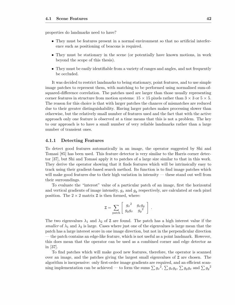
4.1 Scene Features 42
properties do landmarks need to have?
• They must be features present in a normal environment so that no artificial interfer-ence such as positioning of beacons is required.
• They must be stationary in the scene (or potentially have known motions, in workbeyond the scope of this thesis).
• They must be easily identifiable from a variety of ranges and angles, and not frequentlybe occluded.
It was decided to restrict landmarks to being stationary, point features, and to use simpleimage patches to represent them, with matching to be performed using normalised sum-of-squared-difference correlation. The patches used are larger than those usually representingcorner features in structure from motion systems: 15 × 15 pixels rather than 3 × 3 or 5 × 5.The reason for this choice is that with larger patches the chances of mismatches are reduceddue to their greater distinguishability. Having larger patches makes processing slower thanotherwise, but the relatively small number of features used and the fact that with the activeapproach only one feature is observed at a time means that this is not a problem. The keyto our approach is to have a small number of very reliable landmarks rather than a largenumber of transient ones.
4.1.1 Detecting Features
To detect good features automatically in an image, the operator suggested by Shi andTomasi [85] has been used. This feature detector is very similar to the Harris corner detec-tor [37], but Shi and Tomasi apply it to patches of a large size similar to that in this work.They derive the operator showing that it finds features which will be intrinsically easy totrack using their gradient-based search method. Its function is to find image patches whichwill make good features due to their high variation in intensity — these stand out well fromtheir surroundings.
To evaluate the “interest” value of a particular patch of an image, first the horizontaland vertical gradients of image intensity, gx and gy respectively, are calculated at each pixelposition. The 2 × 2 matrix Z is then formed, where:
Z =∑
patch
[
gx2 gxgy
gygx gy2
]
.
The two eigenvalues λ1 and λ2 of Z are found. The patch has a high interest value if thesmaller of λ1 and λ2 is large. Cases where just one of the eigenvalues is large mean that thepatch has a large interest score in one image direction, but not in the perpendicular direction— the patch contains an edge-like feature, which is not useful as a point landmark. However,this does mean that the operator can be used as a combined corner and edge detector asin [37].
To find patches which will make good new features, therefore, the operator is scannedover an image, and the patches giving the largest small eigenvalues of Z are chosen. Thealgorithm is inexpensive: only first-order image gradients are required, and an efficient scan-ning implementation can be achieved — to form the sums
∑
gx2,∑
gxgy,∑
gygx and∑
gy2
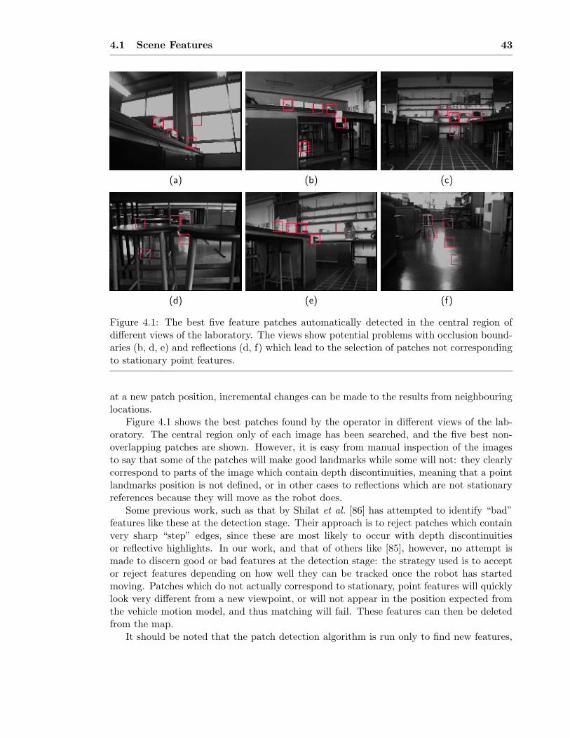
4.1 Scene Features 43
(a) (b) (c)
(d) (e) (f)
Figure 4.1: The best five feature patches automatically detected in the central region ofdifferent views of the laboratory. The views show potential problems with occlusion bound-aries (b, d, e) and reflections (d, f) which lead to the selection of patches not correspondingto stationary point features.
at a new patch position, incremental changes can be made to the results from neighbouringlocations.
Figure 4.1 shows the best patches found by the operator in different views of the lab-oratory. The central region only of each image has been searched, and the five best non-overlapping patches are shown. However, it is easy from manual inspection of the imagesto say that some of the patches will make good landmarks while some will not: they clearlycorrespond to parts of the image which contain depth discontinuities, meaning that a pointlandmarks position is not defined, or in other cases to reflections which are not stationaryreferences because they will move as the robot does.
Some previous work, such as that by Shilat et al. [86] has attempted to identify “bad”features like these at the detection stage. Their approach is to reject patches which containvery sharp “step” edges, since these are most likely to occur with depth discontinuitiesor reflective highlights. In our work, and that of others like [85], however, no attempt ismade to discern good or bad features at the detection stage: the strategy used is to acceptor reject features depending on how well they can be tracked once the robot has startedmoving. Patches which do not actually correspond to stationary, point features will quicklylook very different from a new viewpoint, or will not appear in the position expected fromthe vehicle motion model, and thus matching will fail. These features can then be deletedfrom the map.
It should be noted that the patch detection algorithm is run only to find new features,

4.1 Scene Features 44
(a) (b) (c)
Figure 4.2: Elliptical search regions generated for features. The size of the ellipse dependson the uncertainty of the relative positions of the robot and feature, as will be explained inChapter 5.
which are chosen as the maxima returned. When it is necessary to find a particular feature ina subsequent image, a search is carried out using normalised sum-of-squared-difference: thepatch detection algorithm is not used on the new image. This differs from many structurefrom motion systems where the feature detector is run on each new image: features are foundas local maxima of the particular feature-finding operator, and then correlation matchingis carried out between the features found in the current and previous images, all of whichare local maxima. Some authors [21] have found that requiring all patches matched to bemaxima like this is restrictive, and features can be missed which still give good correlationmatches. This is a good point when applied to our active system, since it is important tokeep track of the same features for as long as possible. Since a search in a particular imageis only for one feature at a time, it makes sense to move straight to correlation matching.
One advantage of applying the feature detector to all images is that most detectors returnfeature locations to sub-pixel accuracy in a natural way. It is more difficult to see how toobtain sub-pixel accuracy from the correlation searching used in our work: interpolationcan be used, but the form of the function to fit to image values depends on the image itself.For speed, and since good accuracy has still been obtained, sub-pixel measurements havenot been used in our work.
4.1.2 Searching For and Matching Features
It will be shown in Chapter 5 that in the localisation system, whenever a measurementis required of a particular feature, a region can be generated in the left and right imageswithin which the feature should lie with a high probability. This means that only that areaof the images need be searched. The region is typically an ellipse centred in the image:some examples are shown in Figure 4.2.
At each position in the region (scanned in raster order), that part of the image iscompared with the patch saved to represent the feature being searched for using the followingnormalised sum-of-squared-difference measure:
C =
∑
patch
[
g1−g1
σ1− g0−g0
σ0
]2
n, (4.1)

4.1 Scene Features 45
Figure 4.3: Features matched with normalised sum-of-squared-difference correlation show-ing the wide changes in viewing distance and direction which can be accommodated.
where g0 and g1 are the image intensity values at corresponding positions in the saved patchand image patch respectively, and g0, g1, σ0 and σ1 are means and standard deviations ofthe intensity across the patches. n is the number of pixels in a patch. This expressionhas the value 0 for a perfect match, with higher values as the difference increases. It wasconsidered essential to use a measure which was normalised with respect to overall intensitychanges, since this gives improved matching over the long periods over which the system isrequired to work, when lighting conditions might change, and also since when working instereo the two cameras will vary somewhat in their output. What the expression actuallymeasures is the average difference in standard deviation above the patch mean intensitybetween corresponding pixels in the patches being compared. The best (lowest) value of Cfound in the search region is accepted as a match if it lies below a threshold (set manuallyat 0.9).
Figure 4.3 shows matches obtained of some features, giving an impression for the sur-prising range of viewpoints which can be matched successfully using the simple patch rep-resentation of features. However, clearly matching can only be expected to succeed forreasonable robot motions, since the patch representation is intrinsically viewpoint-variant— features look different when viewed from new distances or angles. Therefore, we havedefined a criterion for expected visibility based on the differences between the viewpointfrom which the feature was initially seen and a new viewpoint. Figure 4.4 shows the situa-tion: horig is the vector from the head centre to the feature when it was initialised, and h isthat from the head centre at a new vehicle position. The feature is expected to be visibleif the length ratio |h|
|horig|is close enough to 1 (in practice between 5
7 and 75) and the angle
difference β = cos−1((h · horig)/(|h||horig|)) is close enough to 0 (in practice less than 45◦
in magnitude). In the localisation algorithm of Chapter 5, we are in a position to estimateboth of these vectors before a measurement is made, and so attempts are made only to

4.1 Scene Features 46
h
Scene Feature
horig
β
Figure 4.4: The expected visibility of a feature is calculated based on the difference indistance and angle between the viewpoint from which it was initially seen and that fromwhich the current measurement is to be made.
measure features which are expected to be visible. The result is a region of space definedfor each feature from which it should be able to be seen. A features which fails to matchregularly within this region should be deleted from the map.
It should be noted that the patch representing a certain feature is not updated when asuccessful match is made and the feature is re-found — one strategy would be to replace thesaved patch with the region matched to it in the latest image. This would certainly improvethe range of robot movement over which the feature could be tracked, since matching wouldalways be between images taken from closely-spaced viewpoints. However, the problem withthis approach is that the patch tends to drift away from its original position over the feature:a small error in locating the feature at each step (due even to just the pixelation limitation)can lead to a large patch movement over many frames. It is essential that landmarks arestationary features.
4.1.3 Other Feature Types
Two further feature types have been considered for use in the system:
• Planar patch features: several authors [101, 80, 85] have started to use a representationof point features as small planar regions in the 3D world rather than 2D image patches.If this assumption is made, when an attempted measurement is made of a feature, theestimated transformation between the patch plane and the image plane can be usedto warp the saved patch representation into the shape and size in which it will appearfrom the new viewpoint. Clearly this method has the capability to greatly extend therange of robot motion through which particular features can be seen and measured,and this will benefit localisation systems, where it is always an advantage to see thesame landmarks for a long time.
To initialise a feature of this type, it is necessary to assume that it is part of a planarobject (as is certainly approximately the case for many features, such as the markingson a wall), and then to estimate the orientation of that plane. This estimation can

4.2 Fixation 47
be achieved from stereo views of the patch: the difference in its appearance betweenthe left and right camera views provides the information. However, initial trials haveshown that it is difficult to get accurate estimates since the baseline of the activehead is relatively small and the patches do not look very different in the left and rightviews. This problem gets worse the larger the distance from the robot to the feature,but of course with distant features it is less important to know the plane orientationaccurately since views of these features will change relatively little with robot motion.
Shi and Tomasi [85] track features as simple patches, but use affine warpings of thepatches to perform checks on whether features are still “good” in the sense of beingstationary without depth discontinuities. They find that by searching for the bestcorrelation obtained over a range of warpings better rejection of bad features is ob-tained, since correlation scores for good features will get worse to a certain extentdue to viewpoint changes. They do not, however, attempt to estimate the orientationof the planes on which their patches implicitly lie: a search must always take placethrough possible warpings, which is computationally costly.
• Using line features is another possibility, although it has not yet been decided how bestto incorporate these into the map-building system of Chapter 5. Line features wouldrequire new active strategies since it is not so clear where to fixate the camera whenmaking measurements of them. Line features are now commonly used in structurefrom motion systems [83, 21, 103]. Having this capability would make a wider rangeof environmental objects usable as features, and perhaps lead to improvements inautonomous navigation capabilities since line features frequently form the boundariesof obstacles, such as the edges of a door frame.
4.2 Fixation
Fixation means directing a camera or cameras to point directly at a feature in the scene:the camera optic axes will pass through the feature, which will be imaged at the principalpoints. Fixation is one of the main tools of active vision: it means that image processingtakes place always near the centre of images, where discrepancies are most easily dealt with— there is little danger of objects of interest being lost outside image boundaries. Manyvision tasks can be simplified with simple fixated processing. A fixated camera acts as a“pointing stick” towards a feature. In addition, image processing near to the centre of animage reduces reliance on calibration parameters, as will be shown in Section 4.2.2.
In the work in this thesis, fixation is used whenever possible to make measurements ofthe positions of features.
4.2.1 Acquiring Features
Acquiring a new landmark consists of detecting a good patch in an image, then drivingthe active head to fixate the feature so that a measurement can be obtained. The featuredetector of Section 4.1.1 is applied in the left image, and an epipolar line is generated inthe right image: this is the image in the right camera of the line in the scene upon whichthe feature must lie, and it can be determined from the head model and knowledge of thehead angles. A search for a match of the feature is carried out in the close vicinity of this

4.2 Fixation 48
CameraLens
Image Plane
Principal Point u
Image Point uOptic Axis
Angle U
f
Scene Feature
0
Figure 4.5: Relating pixel quantisation errors in the image plane to errors in perceivedangle: this picture shows a two-dimensional view of camera imaging geometry.
line (8 pixels either side of the line). If the match is successful, the 3D location of the pointrelative to the head centre is calculated as in Section 3.3.3. The head angles necessary tofixate the feature are then determined, and the head is driven to this position. The featureshould now be centred in both images: searches for the feature in circular regions near tothe principal points of both are carried out. If the feature is found within a radius of 2pixels of the principal point in both images, the fixation is successful; otherwise, its positionand new head angles are re-calculated, and fixation is re-attempted. If fixation fails severaltimes, the feature is abandoned: a mismatch is usually to blame.
4.2.2 The Accuracy of Fixated Measurements
In image measurements, we can expect to detect features to an accuracy of ±1 pixel innormal circumstances. How does this translate into angular errors in fixation? Referring toFigure 4.5 which shows a simple view of imaging geometry in one plane, we can relate theangle to a scene feature U to its image position u via the equation:
tan U =u − uo
fku,
where f is the focal length of the lens and ku is the pixel density on the image planemeasured in pixels m−1. Differentiating this to determine how small changes δu in u relateto small changes δU in U gives:
sec2 UδU =δu
fku.
Now, when the camera is fixated on a feature, or close to fixation, then the angle a ray fromthat feature makes to the optic axis is very small: U ≈ 0. Hence sec2U ≈ 1 (very closelysince sec2U has a stationary point at U = 0).
⇒ δU =δu
fku.
Since u is measured in pixels, when fixated to an accuracy of 1 pixel then δu = 1.
⇒ δU =1
fku.
For the values of fku and fkv in our cameras, this gives an angular error of:
δU ≈ 0.006rad ≈ 0.3◦ .

4.2 Fixation 49
Depth z (m) γR = −γL (radian) ∆x (m) ∆z (m)
0.2 0.6987 0.0014 0.00190.5 0.3241 0.0022 0.00701 0.1664 0.0044 0.0262 0.08380 0.0086 0.103 0.05594 0.013 0.224 0.04198 0.017 0.405 0.03359 0.022 0.646 0.02799 0.026 0.927 0.02400 0.030 1.28 0.02100 0.034 1.69 0.01866 0.038 2.010 0.01680 0.042 2.615 0.01120 0.064 5.620 0.008400 0.084 10.0
Table 4.1: The uncertainties of the positions of fixation points measured by binocularcameras with inter-ocular spacing 0.338m and angular vergence uncertainties of 0.006rad.
Stereo cameras0.336m baseline
0.2m 0.5m 1m 2m 3m 4m 5m
Figure 4.6: In this scale diagram ellipses show the uncertainties (1σ standard deviation) inrecovered point positions from stereo fixation up to depths of 5m.
Compared to this, angular errors introduced by the active head, whose axes have repeata-bilities with a maximum error of 0.005◦, are negligible. Therefore, in all head measure-ments, an uncertainty of approximately 0.006rad is assigned to angular values obtainedfrom head/image measurements. These uncertainties are directly incorporated into thelocalisation and map-building filter of Chapter 5.
Translating this into uncertainties in the positions of features estimated using fixatedstereo measurements is revealing. Table 4.1 shows the depth (z coordinate) and transverse(x coordinate) uncertainty in estimated feature locations when measurements are made offeatures lying at varying distances directly in front of the robot. Figure 4.6 shows uncer-tainty ellipses to scale for the distances up to 5m. It is clear that while the transverseuncertainty remains small, growing only to 8cm at a distance of 20m, the depth uncertaintygrows rapidly as the feature distance increases. This is because at large depths the two cam-eras are nearly parallel, and the vergence angles change very little for large distance changes:the small uncertainties in vergence measurements translate into large depth uncertainties.It will be seen later how this uncertainty distribution affects navigational capabilities.

4.3 An Example Use of Vision Tools: The Frontal Plane and Gazesphere 50
Frontal Plane
Scene Feature
RestingDirection
Image Point
Steerable Camera
Frontal
Gaze Vector g
Frontal Plane
(a) (b)
Figure 4.7: The frontal plane: (a) shows the mathematical concept of the plane and ele-vating/verging camera. (b) shows how the notional plane relates to our vehicle and activehead.
4.3 An Example Use of Vision Tools: The Frontal Plane andGazesphere
In the second part of this chapter, two ideas will be introduced which provide ways tovisualise the field of view provided by an active camera, and using the methods developedin the first half of the chapter, implementation of an example of simple active-vision basednavigation will be described.
The frontal plane and gazesphere concepts are most easily applied to a single activecamera, and we will demonstrate their use in this case in an active algorithm which recoverssingle-step motions of the robot [24].
• The frontal plane [77] (also referred to as the virtual camera [79]) concept is bestexplained by Figure 4.7. A notional plane is imagined to lie at an arbitrary distance(usually taken as unity) in front of the active camera’s centre of rotation, and perpen-dicular to its resting forward direction. When the active camera moves and fixates ona feature, its optic axis will intersect the plane at a point which can be referred to asthe frontal plane image of the feature. Using the robot’s left camera, once the vector hfrom the left camera optic centre to the feature has been determined and transformedinto the vehicle frame C0, the frontal plane image point (X, Y ) is trivially found fromthe equation:
XY1
∝ hC0 .
Note that a small approximation is made here: that the centre of rotation of theactive camera is the same as its optic centre. This is not quite true due to the offsetsof the active head. However, the optic centre does not move much with rotations of
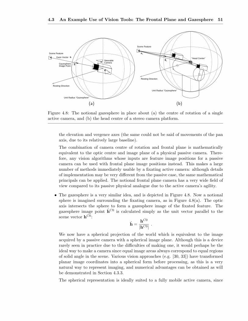
4.3 An Example Use of Vision Tools: The Frontal Plane and Gazesphere 51
Scene Feature
Resting Direction
SteerableCamera
Gaze Vector
Unit Radius "Gazesphere"
GazesphereImage Point
h
h
Scene Feature
Resting Direction
Unit Radius "Gazesphere"
h
h"Head Centre"
G
G
(a) (b)
Figure 4.8: The notional gazesphere in place about (a) the centre of rotation of a singleactive camera, and (b) the head centre of a stereo camera platform.
the elevation and vergence axes (the same could not be said of movements of the panaxis, due to its relatively large baseline).
The combination of camera centre of rotation and frontal plane is mathematicallyequivalent to the optic centre and image plane of a physical passive camera. There-fore, any vision algorithms whose inputs are feature image positions for a passivecamera can be used with frontal plane image positions instead. This makes a largenumber of methods immediately usable by a fixating active camera: although detailsof implementation may be very different from the passive case, the same mathematicalprincipals can be applied. The notional frontal plane camera has a very wide field ofview compared to its passive physical analogue due to the active camera’s agility.
• The gazesphere is a very similar idea, and is depicted in Figure 4.8. Now a notionalsphere is imagined surrounding the fixating camera, as in Figure 4.8(a). The opticaxis intersects the sphere to form a gazesphere image of the fixated feature. Thegazesphere image point hC0 is calculated simply as the unit vector parallel to thescene vector hC0:
h =hC0
|hC0| .
We now have a spherical projection of the world which is equivalent to the imageacquired by a passive camera with a spherical image plane. Although this is a devicerarely seen in practice due to the difficulties of making one, it would perhaps be theideal way to make a camera since equal image areas always correspond to equal regionsof solid angle in the scene. Various vision approaches (e.g. [30, 33]) have transformedplanar image coordinates into a spherical form before processing, as this is a verynatural way to represent imaging, and numerical advantages can be obtained as willbe demonstrated in Section 4.3.3.
The spherical representation is ideally suited to a fully mobile active camera, since

4.3 An Example Use of Vision Tools: The Frontal Plane and Gazesphere 52
it deals naturally with views in all directions, including backwards: the frontal planeconstruction would have to be extended with another plane to deal with rear views.With our camera geometry, controlling just one camera via the elevation and vergenceaxis does not allow it to be directed backwards — however, we can also form the gaze-sphere construction around around the whole active head, as shown in Figure 4.8(b).The head centre now acts as the centre of the gazesphere. From a stereo view of afeature, the head centre vector hG can be calculated, and the intersection of this withthe sphere is the gazesphere image point. Using all its axes like this, the head is ableto reach a field of view which is nearly fully panoramic.
In both of these constructions, the active camera is used as a projective pointing stick,fixation providing simple direction measurements to features which can be simply read fromthe head encoders. This means that both of the representations are effectively calibrated:considering the frontal plane especially, the exact relationship between image positions andscene angles is known. This makes it equivalent to a calibrated passive camera when it isused with passive algorithms.
In the following section we will describe the 8-point algorithm for structure from motionwhich was developed to determine the motion of a passive camera. Then, Sections 4.3.2and 4.3.3 will demonstrate how the frontal plane and gazesphere constructions allow its im-plementation with an active camera to determine robot motion, and discuss the advantagesthis provides.
4.3.1 The 8-Point Algorithm for a Passive Camera
The actual version of the 8-point algorithm used is as described by Weng, Huang and Ahujain [99]. Recent work by Hartley [38] has demonstrated that the 8-point algorithm in thisform still compares well with the best iterative, non-linear methods for tackling two-viewstructure from motion problems.
Consider a camera moving in a scene as shown in Figure 4.9. In a certain discretemotion, its optic centre moves along a vector t in space from OA to OB, and the camerabody is rotated by the matrix RAB. Coordinate frames A and B are aligned with the camerain the initial and final positions respectively. hA is the vector from OA to a point P in thescene, and hB is the vector from OB to P .
We can deduce the simple spatial vector equation:
hA = hB + t.
hA, hB and t are coplanar: they define what is called the epipolar plane. Hence the scalartriple product of these vectors is equal to zero. We write:
hA · (t × hB) = 0.
In the coordinates of frame A:
(
hAAx hA
Ay hAAz
)
E
hBBx
hBBy
hBBz
= 0 , (4.2)

4.3 An Example Use of Vision Tools: The Frontal Plane and Gazesphere 53
O O
y
zx
x
y
z
h h
Scene Point P
e et
B
B
BB
B
B
(X , Y ) BB
AA
A
A
A
A
AA(X , Y )
Figure 4.9: A scene point P is viewed by a camera in two successive positions. The cameramoves along vector t and rotates according to matrix RAB between its initial and finalpositions. (XA, YA) and (XB, YB) are image points on ideal image planes at unit focallength.
where the essential matrix is E = [t×]RAB, in which the antisymmetric matrix [t×] is madefrom the components of the translation vector:
[t×] =
0 −tAz tAytAz 0 −tAx−tAy tAx 0
.
The essential matrix encodes the information about the rotation and translation betweenthe two camera positions. The task is to use image information to determine E and thendecompose it to recover RAB and t.
If we know the ideal image coordinates (XA, YA) and (XB, YB) of the scene point P asseen from the two positions, each scene vector in Equation 4.2 can be replaced with theappropriate image coordinate vector to which it is equal up to a scale factor:
(
XA YA 1)
E
XB
YB
1
= 0. (4.3)
If there are n points in the scene which can be seen from both camera positions, for eachpoint i we can write:
(
XAi YAi 1)
E11 E12 E13
E21 E22 E23
E31 E32 E33
XBi
YBi
1
= 0,

4.3 An Example Use of Vision Tools: The Frontal Plane and Gazesphere 54
where now we have written E in component form. This is equivalent to the equation:(
XAiXBi XAiYBi XAi YAiXBi YAiYBi YAi XBi YBi 1)
E> = 0
where E = ( E11 E12 E13 E21 E22 E23 E31 E32 E33 )>. To compute the essen-tial matrix, we therefore find the vector E which minimizes ||AE||, where the rows of A areconstructed from the image coordinates of each scene point i:
A =
......
......
......
......
...XAiXBi XAiYBi XAi YAiXBi YAiYBi YAi XBi YBi 1
......
......
......
......
...
. (4.4)
E can be found as the unit eigenvector associated with the smallest eigenvalue of A>A aslong as n ≥ 8 — at least eight point correspondences are needed, and the solution will bebetter with more.
The method by which E is decomposed into RAB and t is explained in detail in [99] butwe will briefly outline the procedure, omitting certain sign checks: the unit vector t is foundby minimising ||E>t||. The minimisation can be achieved by singular value decompositionof E> into E> = UWV>. The unit vector will be the right singular vector Vi associated withthe smallest singular value, which should be zero or close to zero. The rotation matrix RAB
is determined by minimising ||RAB>[−t×] − E>||.Once R and t have been calculated, the 3D scene positions or structure of all the n
features matched between the two viewpoints can be found. This can be done simply byback-projecting rays from the camera in its two positions according to each feature’s imagecoordinates and finding their intersection.
So a summary of what the 8-point algorithm does: as a passive camera moves on atrajectory through a scene, if between two positions on the trajectory we can match atleast eight scene points in the image plane, we are able to calculate the interim rotationand direction of translation of the camera as well as the 3D scene positions of the referencefeatures. Two points to note are:
• The rotation, translation and structure recovered are Euclidean only if the camera iscalibrated (as the frontal plane representation is). If we do not know explicitly all thecomponents of its camera calibration matrix C then these quantities can be determinedonly up to a projective ambiguity.
• The algorithm cannot recover the absolute scale of movements — it returns only aunit translation vector describing the direction of motion. The structure calculatedhas the same ambiguity.
4.3.2 The 8-Point Algorithm in The Frontal Plane
Method
The active implementation of the algorithm is straightforward using the ideas developed upto now. The frontal plane idea is used to create the analogue of a fixed wide-angle cameraattached to the vehicle. By operating the 8-point algorithm on point correspondences inthe frontal plane when the vehicle makes a discrete motion from an initial to a final positionwe can hence determine its rotation and translation.

4.3 An Example Use of Vision Tools: The Frontal Plane and Gazesphere 55
• In the initial position the scene is examined for prominent features by the activecamera in a wide field of view.
• Features are chosen by hand or automatically; for each one an image patch is savedand the active camera fixates it via the iterative search procedure described in Sec-tion 4.2.1.
• Once fixation is achieved, the head angles θe and θv from odometry are used tocalculate the frontal plane image position of each feature.
• When a sufficient number of features has been identified from the initial position thevehicle is free to drive somewhere new. Generally, although only eight matches arerequired as a minimum, more features than this will be identified from the initialposition to improve accuracy and allow for potential matching failures.
• After moving, as many features as possible are re-found via correlation matching andre-fixated iteratively.
• The head angles at fixation are used to calculate new frontal plane coordinates forthe features.
• Finally the set of successfully matched frontal plane coordinates is passed to the8-point algorithm which calculates the rotation and direction of translation of thevehicle.
Experiments
Several experiments with known motions of the vehicle were performed to verify the correctoperation of the system and investigate its accuracy. Figure 4.10 shows the motions whichwere used.
FinishStartFinish Start
Finish
Start Start Finish
(a) (b) (c) (d)
Figure 4.10: The vehicle motions used in Experiments 1 (a), 2 (b,c) and 3 (d).
Experiment 1: translation and rotation in the ground plane. In the first experi-ment the vehicle was moved on the ground plane as shown in Figure 4.10(a) with translationtowards its right and backwards, and a rotation to the left measured as 30◦. The directionof translation was not measured in this case since due to the rotation of the vehicle it was
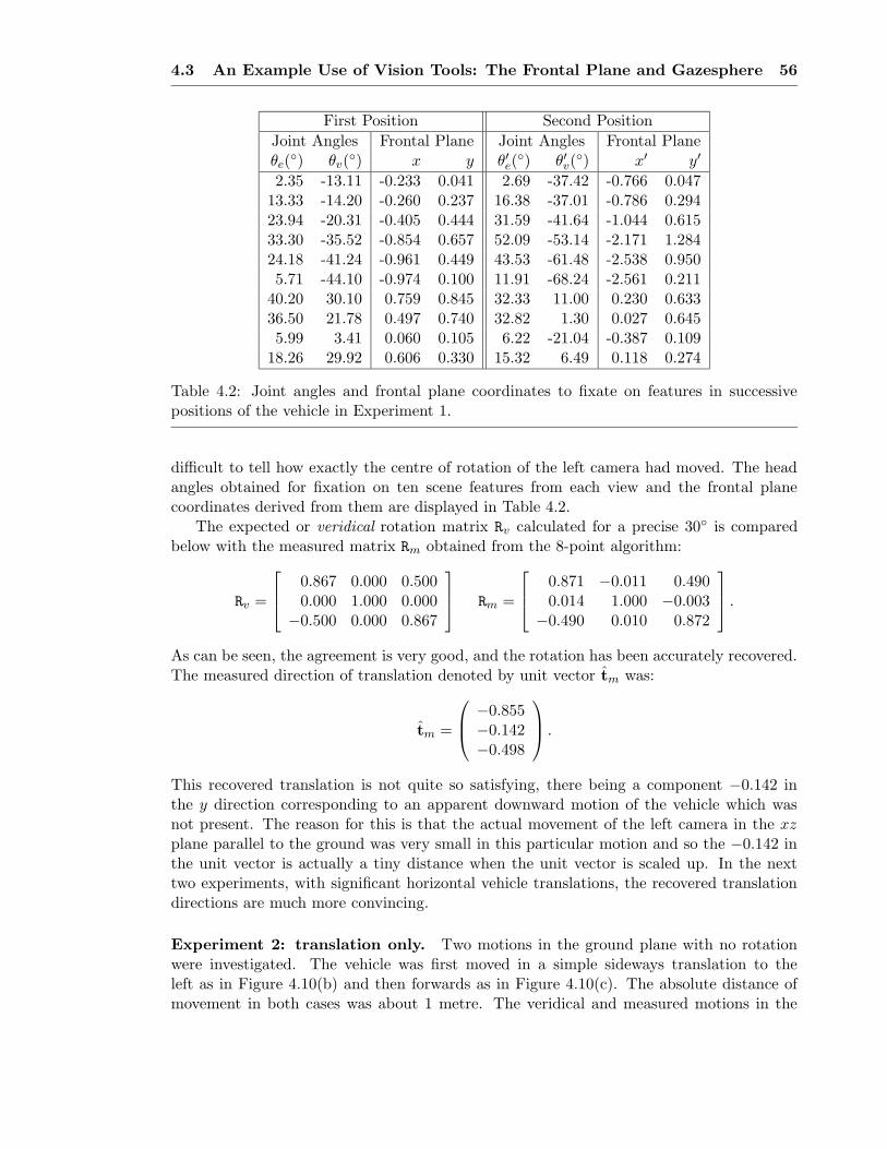
4.3 An Example Use of Vision Tools: The Frontal Plane and Gazesphere 56
First Position Second Position
Joint Angles Frontal Plane Joint Angles Frontal Planeθe(
◦) θv(◦) x y θ′e(
◦) θ′v(◦) x′ y′
2.35 -13.11 -0.233 0.041 2.69 -37.42 -0.766 0.04713.33 -14.20 -0.260 0.237 16.38 -37.01 -0.786 0.29423.94 -20.31 -0.405 0.444 31.59 -41.64 -1.044 0.61533.30 -35.52 -0.854 0.657 52.09 -53.14 -2.171 1.28424.18 -41.24 -0.961 0.449 43.53 -61.48 -2.538 0.9505.71 -44.10 -0.974 0.100 11.91 -68.24 -2.561 0.211
40.20 30.10 0.759 0.845 32.33 11.00 0.230 0.63336.50 21.78 0.497 0.740 32.82 1.30 0.027 0.6455.99 3.41 0.060 0.105 6.22 -21.04 -0.387 0.109
18.26 29.92 0.606 0.330 15.32 6.49 0.118 0.274
Table 4.2: Joint angles and frontal plane coordinates to fixate on features in successivepositions of the vehicle in Experiment 1.
difficult to tell how exactly the centre of rotation of the left camera had moved. The headangles obtained for fixation on ten scene features from each view and the frontal planecoordinates derived from them are displayed in Table 4.2.
The expected or veridical rotation matrix Rv calculated for a precise 30◦ is comparedbelow with the measured matrix Rm obtained from the 8-point algorithm:
Rv =
0.867 0.000 0.5000.000 1.000 0.000
−0.500 0.000 0.867
Rm =
0.871 −0.011 0.4900.014 1.000 −0.003
−0.490 0.010 0.872
.
As can be seen, the agreement is very good, and the rotation has been accurately recovered.The measured direction of translation denoted by unit vector tm was:
tm =
−0.855−0.142−0.498
.
This recovered translation is not quite so satisfying, there being a component −0.142 inthe y direction corresponding to an apparent downward motion of the vehicle which wasnot present. The reason for this is that the actual movement of the left camera in the xzplane parallel to the ground was very small in this particular motion and so the −0.142 inthe unit vector is actually a tiny distance when the unit vector is scaled up. In the nexttwo experiments, with significant horizontal vehicle translations, the recovered translationdirections are much more convincing.
Experiment 2: translation only. Two motions in the ground plane with no rotationwere investigated. The vehicle was first moved in a simple sideways translation to theleft as in Figure 4.10(b) and then forwards as in Figure 4.10(c). The absolute distance ofmovement in both cases was about 1 metre. The veridical and measured motions in the

4.3 An Example Use of Vision Tools: The Frontal Plane and Gazesphere 57
first motion, where 11 feature correspondences were obtained, were:
tv =
1.0000.0000.000
, tm =
0.999−0.003
0.051
Rv =
1.000 0.000 0.0000.000 1.000 0.0000.000 0.000 1.000
, Rm =
1.000 −0.004 −0.0090.004 1.000 0.0060.009 −0.006 1.000
.
For the second translation, the veridical and measured motion estimated for 12 correspon-dences were:
tv =
0.0000.0001.000
, tm =
−0.016−0.003
1.000
Rv =
1.000 0.000 0.0000.000 1.000 0.0000.000 0.000 1.000
, Rm =
1.000 0.020 −0.042−0.020 1.000 −0.009
0.041 0.010 1.000
.
It can be seen that for both of these motions the measured quantities are very close to theexpected axial unit translation vectors and identity rotation matrices.
Experiment 3: rotation and translation out of the ground plane. To demonstratethat recoverable motions are not confined to the ground plane, the front of the vehicle wasraised up so that the vehicle’s base made an angle of 10◦ with the ground as in Figure 4.10(d).Using 19 matched points, the recovered motion was:
tm =
0.1090.2090.972
Rv =
1.000 0.000 0.0000.000 0.985 0.1740.000 −0.174 0.985
, Rm =
1.000 0.005 0.001−0.005 0.983 0.183−0.000 −0.183 0.983
.
We have compared the measured rotation with the matrix calculated for a precise 10◦
rotation in the vertical yz plane and the agreement is again good.
4.3.3 The 8-Point Algorithm in the Gazesphere
The 8-point algorithm can be adapted slightly to work with spherical image coordinates,and this presents two advantages:
• Features can now lie in any direction relative to the centre of rotation, not just for-wards. This means that matching can be achieved over any rotations of the robot.
• The improved numerical conditioning of the spherical representation means that theaccuracy of motions recovered from the gazesphere is slightly better than from thefrontal plane.

4.3 An Example Use of Vision Tools: The Frontal Plane and Gazesphere 58
Fixation Angles From Vehicle Positions (radians)Feature A B C D
Coordinates θe θv θe θv θe θv θe θv
(3, 2, 5) 0.380506 0.508267 0.380506 0.748327 0.588003 0.693981 0.755969 1.038493(6, 0, 8) 0.000000 0.643501 0.000000 0.785398 0.000000 0.785398 0.000000 1.343997(4, 4, 10) 0.380506 0.355603 0.380506 0.508267 0.463648 0.420534 0.679674 0.965252(2, -1, 8) -0.124355 0.243161 -0.124355 0.460554 -0.165149 0.317663 -0.199347 0.900036(-1, 0, 12) 0.000000 -0.083141 0.000000 0.083141 0.000000 -0.099669 0.000000 0.620249(-2, 2, 10) 0.197396 -0.193658 0.197396 0.000000 0.244979 -0.237941 0.214233 0.484350(-4, -2, 11) -0.179853 -0.343581 -0.179853 -0.177013 -0.218669 -0.409352 -0.174969 0.353742(-5, 3, 8) 0.358771 -0.529470 0.358771 -0.337675 0.463648 -0.640522 0.294249 0.135875(-4, -2, 5) -0.380506 -0.638865 -0.380506 -0.355603 -0.588003 -0.837215 -0.275643 -0.000000(-7, 1, 5) 0.197396 -0.941243 0.197396 -0.775594 0.321751 -1.146485 0.108360 -0.225513
Table 4.3: The head angles for precise fixation on the scene points from the four vehiclevehicle positions.
To use the 8-point algorithm with spherical coordinates, it is necessary just to replacethe image vectors of Equation 4.3 with gazesphere image vectors to give the constraintprovided by each feature match as:
(
hC0Ax hC0
Ay hC0Az
)
E
hC0Bx
hC0By
hC0Bz
= 0 . (4.5)
Hence the rows of matrix A as in Equation 4.4 are now constructed from spherical coordinatecomponents:
A =
.
.
....
.
.
....
.
.
....
.
.
....
.
.
.
hC0Axi
hC0Bxi
hC0Axi
hC0Byi
hC0Axi
hC0Bzi
hC0Ayi
hC0Bxi
hC0Ayi
hC0Byi
hC0Ayi
hC0Bzi
hC0Azi
hC0Bxi
hC0Azi
hC0Byi
hC0Azi
hC0Bzi
.
.
....
.
.
....
.
.
....
.
.
....
.
.
.
(4.6)We can then go on as before to find E and decompose it to recover R and t.
Spherical Coordinates Versus Frontal Plane Coordinates: A Comparison UsingSimulated Data
A set of tests with fabricated data was performed to verify the numerical advantages ofusing spherical coordinates with the 8-point algorithm.
A set of ten 3D feature points in space was invented and the vehicle imagined to moveon the ground plane between four positions amongst them (chosen such all the points werevisible at all times). Figure 4.11 shows the situation from a top-down viewpoint (the featurepoints also had heights as denoted in their coordinates). From each of the vehicle positionsA, B, C and D, the head angles necessary for fixation on all of the features were calculated.These are shown in Table 4.3.
Gaussian noise of magnitude equal to the noise expected in angular head measurements(see Section 4.2.2) was added to the angles, and they were converted into both frontal planeand spherical coordinates as explained earlier. Matched sets of these coordinates for themotions A → B, A → C and A → D were then fed to the 8-point algorithm to see how wellthe motions were recovered with the different coordinate types.

4.3 An Example Use of Vision Tools: The Frontal Plane and Gazesphere 59
(3, 2, 5)
(−5, 3, 8)
(−7, 1, 5)
z
x
A
C
BD
(6, 0, 8)
(4, 4, 10)
(2, −1, 8)
(−1, 0, 12)
(−2, 2, 10)
(−4, −2, 11)
(−4, −2, 5)
Figure 4.11: An above-head view of the vehicle and feature positions used in the numericalcomparison of spherical and frontal plane coordinates.
The true motions of the ideal vehicle, described as a unit translation vector t and arotation matrix R were:
A → B : t =
−1.0000000.0000000.000000
R =
1.000000 0.000000 0.0000000.000000 1.000000 0.0000000.000000 0.000000 1.000000
A → C : t =
0.0000000.0000001.000000
R =
1.000000 0.000000 0.0000000.000000 1.000000 0.0000000.000000 0.000000 1.000000
A → D : t =
1.0000000.0000000.000000
R =
0.707107 0.000000 −0.7071070.000000 1.000000 0.0000000.707107 0.000000 0.707107
For the noisy data and the frontal plane coordinate system, the recovered motions were:
A → B : t =
−0.9998620.0080750.014543
R =
0.999944 −0.000866 −0.0105910.000946 0.999972 0.0074670.010584 −0.007476 0.999916

4.4 Conclusion 60
A → C : t =
−0.023559−0.009083
0.999681
R =
0.999971 0.000830 0.007504−0.000860 0.999992 0.003902−0.007501 −0.003909 0.999964
A → D : t =
0.997672−0.038149−0.056524
R =
0.699795 −0.003049 −0.7143370.017624 0.999760 0.0129980.714126 −0.021685 0.699681
The motions recovered using spherical coordinates were:
A → B : t =
−0.9998190.0064720.017901
R =
0.999964 −0.000233 −0.0084810.000277 0.999987 0.0051370.008480 −0.005139 0.999951
A → C : t =
−0.022316−0.008430
0.999715
R =
0.999974 0.000638 0.007145−0.000664 0.999993 0.003719−0.007143 −0.003724 0.999968
A → D : t =
0.998009−0.033777−0.053257
R =
0.700428 −0.003897 −0.7137130.015756 0.999826 0.0100040.713549 −0.018252 0.700367
It can be seen that the spherical coordinates perform consistently slightly better thanthe frontal plane coordinates with exactly the same input data, being closer to the perfectvalues in nearly all cases. The reason for this is the better numerical conditioning of thespherical coordinates which makes them more suitable for constructing the rows of thematrix A which is decomposed to find E. The spherical coordinate values all lie in the range0 → 1 whereas the frontal plane coordinates can be unlimited in size and tend to ∞ forfeatures at large angles. Small angular errors will lead to large frontal plane position errorsat these positions. With spherical coordinates, a certain angular error will lead to the samechange in coordinate values whatever the position of the feature — the noise in the system,whose form is not specified in the 8-point algorithm, is dealt with better in this case.
4.4 Conclusion
This chapter has presented the vision tools for dealing with features, and shown how thefrontal plane and gazesphere concepts can be used to implement a previously developednavigation algorithm. As is stands, however, the 8-point algorithm is not much use forextended periods of vehicle navigation, considering as it does only single motions. A muchmore difficult problem is constructing a system which can estimate compound motionsfrom the same kind of feature measurements. It is also desirable to be able to make useof whatever number of measurements is available: the 8-point algorithm is unsuitable forpractical active navigation since the robot must fixate in turn upon at least eight featuresto determine its position — a time-consuming process. A measurement of just one featureshould be sufficient to provide at least some information on motion.
In the next chapter, we will present the main part of the map-building and localisationalgorithm developed to solve these problems for long-term robot navigation.
5Map Building and Sequential
Localisation
Navigating in unknown surroundings inherently couples the processes of building a mapof the area and calculating the robot’s location relative to that map. In the previouschapter, an active implementation of a structure from motion algorithm was demonstratedwhich allows the calculation of a single motion of the robot. This method, however, hasno natural extension to compound motions, where it is desirable to calculate the robot’slocation sequentially relative to a continuously updated map of features. It is necessary toconsider the uncertainties introduced into the map by potential noise sources in the robotmotion and measurement process.
In this chapter we will describe the map-building and localisation algorithm which webelieve is key to a navigation system using active vision. The algorithm relies on thefamiliar Kalman Filter, but the particular way it has been used has been designed aroundthe requirements of our robot navigation system. These requirements are that in previouslyunknown environments, maps of features can be automatically generated which are usefuland efficient, in terms of providing landmarks which are easy and relevant to refer to, andconsistent and long-lasting, meaning that they can be used for long periods of navigationin the same area. It is also a requirement that the localisation method is applicable toreal robot tasks, where particular goals must be achieved, whether specified by a humanoperator or generated by the robot itself.
5.1 Kalman Filtering
The Kalman Filter is a general statistical tool for the analysis of time-varying physicalsystems in the presence of noise. A system is modelled by a state vector x which has entries
5.1 Kalman Filtering 62
for each of the quantities of interest. The passage of time is divided into small intervals∆t, and knowledge of the expected evolution of the state vector is encapsulated in the statetransition function f .
The filter permits continuous and efficient estimation of x as the system evolves, incor-porating the information provided by any measurements z which are made of quantitiesdepending on the state. The current state estimate is stored in the vector x, and the covari-ance matrix P, which is square and symmetric with dimension of the number of elementsin x, represents the uncertainty in x. If the dependence of both f and the measurementfunction h on x is linear, and the statistical distribution of noise in the state transition andmeasurements is Gaussian, then the solution produced is optimal.
5.1.1 The Extended Kalman Filter
The Extended Kalman Filter (EKF) is a simple extension of the Kalman Filter to copewith systems whose state transition and measurement functions are non-linear, or whosenoise distributions are non-Gaussian. This is true of most physical systems to which thefilter has been applied, and it acts only as an approximation in these cases, where thedownside of its efficiency is oversimplification of the mathematical forms of the functionsand distributions involved. Usually the results are quite adequate, but in some recentvision applications, such as tracking the outlines of rapidly moving objects against clutteredbackgrounds, the Kalman Filter has been found to fail (in this case due to its inability touse multi-modal distributions to represent multiple hypotheses about the location of anobject) and replacement algorithms have been developed [45]. In our system, the EKF hasbeen found to work well, although it has been important to be careful with some aspects offormulation, as will be explained later.
Prediction
In a step of time during which no measurements are made, our estimate of the state of asystem changes according to the state transition function f describing the dynamics. Thecovariance matrix changes reflecting the increase in uncertainty in the state due to noise Q
in the state transition (due to random effects or factors which are not accounted for in thedynamic model). Both f and Q depend on u, the current vehicle control vector specifyingdemanded velocity and steering angle. The label k denotes an incrementing time step.
x(k + 1|k) = f(x(k|k),u(k)) , (5.1)
P(k + 1|k) =∂f
∂x(k|k)P(k|k)
∂f
∂x
>
(k|k) + Q(k) . (5.2)
Update
When a measurement is made, the state estimate improves with the new information and theuncertainty represented by P will reduce. ν is the difference between the actual measurementz and the prediction h calculated from the current state, and is called the innovation. R isthe covariance matrix of the noise in the measurement. The update equations for state andcovariance are:
x(k + 1|k + 1) = x(k + 1|k) + W(k + 1)ν(k + 1) , (5.3)

5.2 Simultaneous Map-Building and Localisation 63
P(k + 1|k + 1) = P(k + 1|k) − W(k + 1)S(k + 1)W>(k + 1) , (5.4)
where the innovation is
ν(k + 1) = z(k + 1) − h(x(k + 1|k)) , (5.5)
W, the Kalman gain, is
W(k + 1) = P(k + 1|k)∂h
∂x
>
(k|k)S−1(k + 1) , (5.6)
and S, the innovation covariance is
S(k + 1) =∂h
∂x(k|k)P(k + 1|k)
∂h
∂x
>
(k|k) + R(k + 1) . (5.7)
The innovation covariance represents the uncertainty in ν, the amount by which a truemeasurement differs from its predicted value.
5.2 Simultaneous Map-Building and Localisation
5.2.1 Frames of Reference and the Propagation of Uncertainty
In a map-building and localisation system, the quantities of interest are the coordinates ofmap features and the location of the robot. It is these which will form the state vector ofthe filter.
When deciding upon the exact form of the filter, the issue of coordinate frames and theirsignificance was considered in detail. Consider navigation around a restricted area such as aroom: certainly there is no need to know about position or orientation relative the world as awhole, but just about the relative location of certain features of the room (walls, doors, etc.).This initially suggested a completely robot-centred approach to navigation: the positions ofthese features would be estimated in a robot-centred coordinate frame at all times, and therobot’s location would not be explicitly described. A forward motion of the robot wouldappear simply as a backward motion of the features. This approach is attractive becauseit seems to encapsulate all the information that is important for navigation in initiallyunknown surroundings. However, such an approach cannot explicitly answer questions suchas “how far has the robot moved between points A and B on its trajectory?”, or even enablethe robot to perform a task as simple as returning to its starting position after carrying outa particular motion. These capabilities are essential in goal-directed performance.
Therefore, the approach chosen explicitly estimates the robot and feature positionsrelative to a world frame while maintaining covariances between all the estimates. Thisprovides a way to answer these questions while retaining all the functionality of the robot-centred method, since it is possible at any stage to re-zero the coordinate frame to the robot,as we will show in Section 5.3.8. The extra information held in the explicit robot state andits covariances with the feature estimates codes the registration information between anarbitrary world coordinate frame or map and the structure of the feature map the robothas built itself. This representation allows for the inclusion of prior information given tothe robot about the world, as will be shown in Chapter 7.

5.2 Simultaneous Map-Building and Localisation 64
Autonomous map-building is a process which must be carefully undertaken. A mapwhich is made by a traveller or robot who does not have some external measure of ego-motion is fundamentally limited in its accuracy. The problem is caused by the compounderrors of successive measurements. Consider, for example, a human given the task of drawinga very long, straight line on the ground, but equipped with only a 30cm ruler, and unable touse any external references such as a compass or the bearing of the sun. The first few metreswould be easy, since it would be possible to look back to the start of the line when aligningthe ruler to draw a new section. Once this had gone out of view, though, only the recentlydrawn nearby segment would be available for reference. Any small error in the alignment ofthis segment would lead to a misalignment of new additions. At a large distance from thestarting point, the cumulative uncertainty will be great, and it will be impossible to say withany certainty whether the parts of line currently being drawn were parallel to the originaldirection. Changing the measurement process could improve matters: if, for instance, flagscould be placed at regular intervals along the line which were visible from a long way, thencorrect alignment could be better achieved over longer distances. However, eventually theoriginal flags would disappear from view and errors would accumulate — just at a slowerrate than before.
Something similar will happen in a robot map-building system, where at a certain timemeasurements can be made of only a certain set of features which are visible from thecurrent position — probably these will in general be those that are nearby, but there areusually other criteria as discussed in Section 4.1.2, such as occlusion or maximum viewingangle. It will be possible to be confident about the robot’s position relative to the featureswhich can currently be seen, but decreasingly so as features which have been measured inthe more distant past are considered. Should the map-building algorithm chosen accuratelyreflect this if the maps generated are to be consistent and useful for extended periods?We argue yes, and show how this can be achieved by implementing localisation and map-building using a single Kalman Filter, where a large state vector contains all the quantitiesof interest (the robot and feature positions) and a large covariance matrix stores the relateduncertainties of all of these.
In the majority of previous approaches to robot navigation and sequential structure frommotion, (e.g. [36, 10, 8, 27]), separate filters have been used for the robot position and thatof each of the features (or further simplified schemes, where, for instance, the robot stateis not estimated explicitly with a covariance but is calculated by a least squares fit of themost recently measured features to those in the map). This approach is certainly attractivedue to its reduction of the computational complexity of building and updating a map. Eachparticular estimated state vector — the small number of coordinates describing the locationof the robot or one feature — is stored along with the small covariance matrix describing theuncertainty in that estimate. What are not stored, however, are the covariance cross-termsrelating the estimates of the coordinates of different features or the robot. It has been arguedpreviously [91, 92, 93] that this is not sufficient for fully effective map-building, althoughit has appeared to be effective in many demonstrations. What these demonstrations havefailed to show, however, is the production of maps that are useful for any extended periodsof navigation and the performance of robot tasks. Maps built in this way without fullconsideration of the uncertainties involved are prone to inconsistency. A familiar state ofaffairs is the observation that the trajectory calculated by a robot which has moved in alooped path does not join up at the ends — this is reported in work by both Harris and

5.2 Simultaneous Map-Building and Localisation 65
Pike [36] and Bouget and Perona [10]. An experiment will be reported in Section 5.4.4 laterin this chapter which demonstrates how the full covariance approach greatly improves onthis.
Some previous authors have tackled the problem of producing real-time implementationsof map-building using the full covariance matrix. McLauchlan’s Variable State-DimensionFilter [63, 64] ingeniously reduces the complexity of updates by operating on the inverse ofthe covariance matrix (often called the information matrix), which in certain problems has asimple block-diagonal form. This is indeed the case with map-building in cases where thereis no prior information about the motion of the observer — reconstruction of scenes fromarbitrary video sequences for instance. It is not yet clear whether additional informationsuch as robot odometry data can be incorporated into this simple form. Csorba [23] haspresented an efficient algorithm which reduces the complexity of full covariance updateswhile reducing accuracy slightly to within a bounded range.
Our approach to the potential problem of the computational complexity of maintaininga large coupled filter is described in Chapter 6, where an algorithm is described which canreduce the amount of processing to be performed when making repeated measurements ofjust one feature in the map to a small, constant amount, by postponing the full, but exact,update of the whole state until the robot has stopped moving and has some unutilisedprocessing time.
5.2.2 Map-Building in Nature
It is interesting to ponder the way that humans and animals deal with the map-buildingproblem. It certainly does not seem that we store the equivalent of a huge covariance matrixrelating the uncertainties in our estimates of the positions of all the features in a certainarea. Within one part of that area, for example on a street in the middle of a large familiarcity, it might be difficult to point in the direction of another street on the other side of thecity, or to estimate its distance, but very easy to find the way there if necessary — fromthe current position, some local landmarks would enable the first street along the journeyto be found, which would lead to the next, and so on to the final destination. Of course,a city is a simplified environment because generally paths through it are limited to thegrid of streets; but humans make great use of the local relations between landmarks —it is only necessary to be able to find the few nearby points of interest from the currentposition. Canonical paths [69] are standard choices of route which will ease navigation, andthese have been noted in many situations. Human navigators prior to the latter part of theeighteenth century used to “sail the parallels” [32], meaning that voyages were composedof straightforward north/south or east/west sections where navigation was simpler, ratherthan the more direct alternatives. We are also reminded of Leonard’s suggestion that inrobot navigation map contact [52] is often more important than other criteria, such as shortdistance, when planning a path.
The relationship between the positions of features is exactly what is monitored by thelarge covariance matrix in our map-building algorithm, but perhaps more information isbeing stored than is truly necessary. Full consideration of the relationship between featuresin a local area certainly seems worth keeping, but is it really important to know individuallyabout the relationship between each of these features and a particular distant one, as iscurrently the case? The sort of environment is relevant: in open country, where there
5.3 The Map-Building and Localisation Algorithm 66
are few landmarks, it is more important to know about how each relates to the others,since it may be necessary to “strike out” over a long distance between them without beingable to refer to others along the way. For a robot operating in a relatively plain indoorenvironment, the situation is similar, since the robot will be aware of only a sparse map ofinteresting features — though in future systems, use of more advanced representations andfeature types such as lines and planes might give the robot a human’s instinctive grasp ofthe geometry of a room and his or her position in it.
Our system could become more like the apparent human one then by selectively storingfeature relationships. In an indoor environment, they could be grouped into rooms forinstance, and adjoining rooms coupled in some way. The covariance matrix would becomemore diagonal (if the features are listed in it in room order).
5.3 The Map-Building and Localisation Algorithm
5.3.1 The State Vector and its Covariance
Current estimates of the locations of the robot and the scene features which are knownabout are stored in the system state vector x, and the uncertainty of the estimates in thecovariance matrix P. These are partitioned as follows:
x =
xv
y1
y2...
, P =
Pxx Pxy1Pxy2
. . .Py1x Py1y1
Py1y2. . .
Py2x Py2y1Py2y2
. . ....
......
. (5.8)
x has 3(n + 1) elements, where n is the number of known features. P is symmetric, withsize 3(n + 1)× 3(n + 1). x and P will change in dimension as features are added or deletedfrom the map. xv is the robot position estimate, and yi the estimated 3D location of theith feature:
xv =
zx
φ
, yi =
Xi
Yi
Zi
.
These coordinates are all in the world frame W , but the frame superscript is dropped forclarity.
5.3.2 Filter Initialisation
The usual way to initialise the system is with no knowledge of any scene features, and withthe world coordinate frame defined to be aligned with the robot’s starting position. Therobot’s coordinates are z = 0, x = 0, φ = 0 by definition — and since these are knownexactly, the starting covariance matrix has all entries equal to zero:
x =
000
, P =
0 0 00 0 00 0 0
. (5.9)

5.3 The Map-Building and Localisation Algorithm 67
5.3.3 Moving and Making Predictions
The robot’s motion is discretised into steps of time interval ∆t, with an incrementing labelk affixed to each. ∆t is set to be the smallest interval at which changes are made to thevehicle control inputs v and s, allowing the motion model of Section 3.4 to be used. Aftera step of movement, a new state estimate and covariance are produced:
x(k + 1|k) =
fv(xv(k|k),u(k)y1(k|k)y2(k|k)
...
(5.10)
P(k + 1|k) =
∂fv∂xv
Pxx(k|k) ∂fv∂xv
>+ Q(k) ∂fv
∂xvPxy1
(k|k) ∂fv∂xv
Pxy2(k|k) . . .
Py1x(k|k) ∂fv∂xv
>Py1y1
(k|k) Py1y2(k|k) . . .
Py2x(k|k) ∂fv∂xv
>Py2y1
(k|k) Py2y2(k|k) . . .
......
...
(5.11)
where fv and Q(k) are as defined in Equation 3.22. This new covariance matrix is formulated
from the usual EKF prediction rule P(k + 1|k) = ∂f∂xP(k|k) ∂f
∂x
>+ Q(k), where ∂f
∂xis the full
state transition Jacobian:
∂f
∂x=
∂fv∂xv
O O . . .
O I O . . .O O I . . ....
......
.
5.3.4 Predicting a Measurement and Searching
Making a measurement of a feature i consists of determining its position relative to therobot: technically, the components in the robot frame C0 of the vector hG from the headcentre to the feature. The function of the true robot and feature positions giving theCartesian components of this vector is:
hC0Gi =
hC0Gix
hC0Giy
hC0Giz
=
cos φ(Xi − x) − sin φ(Zi − z)Yi − H
sin φ(Xi − x) + cos φ(Zi − z)
. (5.12)
The predicted measurement of a feature at the current robot position is therefore cal-culated from the above equation with the state estimates xv and yi substituted for xv andyi. When a measurement of this vector is made, the innovation covariance (which is thecovariance of the difference between the true and measured values) will be given by:
ShGi =∂hGi
∂xP∂hGi
∂x
>
+ RL
=∂hGi
∂xvPxx
∂hGi
∂xv
>
+ 2∂hGi
∂xvPxyi
∂hGi
∂yi
>
+∂hGi
∂yiPyiyi
∂hGi
∂yi
>
+ RL . (5.13)
RL is the measurement noise (see Section 5.3.5) transformed into Cartesian measurementspace.

5.3 The Map-Building and Localisation Algorithm 68
To measure the feature, the active head is driven to the angles necessary for fixation onthis estimated relative feature location (calculated as described in Section 3.3.3). In cameracentred coordinates (reference frames L and R respectively), the vectors hL and hR fromthe camera optic centres to the feature and their covariances PhL
and PhR(calculated by
transforming ShGi) are formed. Both of these vectors will have zero x and y componentssince at fixation the z-axis-defining optic axes pass through the feature. Considering theleft camera, image projection is defined by the the usual equations:
uL = − fkuhL
Lx
hLLz
+ u0 and vL = − fkv
hLLy
hLLz
+ v0 . (5.14)
The covariance matrix of the image vector uL =
(
uL
vL
)
is given by UL = ∂uL
∂hLL
PhLL
∂uL
∂hLL
>.
The value of the Jacobian at hLLx = hL
Ly = 0 is
∂uL
∂hLL
=
[
−fku
hLz0 0
0 −fkv
hLz0
]
.
Specifying a number of standard deviations (typically 3), UL defines an ellipse in the leftimage which can be searched for the feature patch representing the feature in question. Thesame procedure is followed in the right image (Figure 4.2 shows some typically generatedsearch regions). Limiting search for feature patches to these small areas maximises com-putational efficiency and minimises the chance of obtaining mismatches. If the feature issuccessfully matched in both images, the final value of the measurement hC0
Gi is calculatedfrom the expression in Section 3.3.3.
5.3.5 Updating the State Vector After a Measurement
Before processing a measurement it is transformed into an angular form:
hi =
αi
ei
γi
=
tan−1 hGix
hGiz
tan−1 hGiy
hGiρ
tan−1 I2hGi
, (5.15)
where hGi is the length of vector hGi and hGiρ =√
hGix2 + hGiz
2 is its projection onto thexz plane. I is the inter-ocular separation of the active head. These angles represent thepan, elevation and vergence angles respectively of an ideal active head positioned at thehead centre and fixating the feature, “ideal” here meaning a head that does not have theoffsets that the real head had — in terms of Figure 2.1(b), this would mean that vectors nand c would be zero, with p purely along the elevation axis. Now αi, ei and γi will be veryclose to the actual pan, elevation and vergence angles of the real active head at fixation,but accuracy is gained by taking account of all the head offsets in this way.
The reason for using an angular measurement representation at all is that it allowsmeasurement noise to be represented as a constant, diagonal matrix. The largest error inmeasurements is in the accuracy with which features can be located in the image centre— the rule used is that a successful fixation lock-on has been achieved when the feature
5.3 The Map-Building and Localisation Algorithm 69
is located within a radius of two pixels from the principal point in both images. Thisrepresents an angular uncertainty of around 0.3◦ (see Section 4.2.2), and Gaussian errors ofthis standard deviation are assigned to αi, ei and γi. The angular errors in measurementsfrom the head axis encoders, which have repeatabilities of size 0.005◦, are much smallerthan this and can be neglected. The measurement noise covariance matrix is therefore:
R =
∆α2 0 00 ∆e2 00 0 ∆γ2
. (5.16)
With a diagonal R, measurements αi, ei and γi are independent. This has two advantages:first, potential problems with bias are removed from the filter update by representing mea-surements in a form where the noise can closely be modelled as Gaussian. Second, themeasurement vector hi can be decoupled, and scalar measurement values used to updatethe filter in sequence. This is computationally beneficial since it is now not necessary toinvert any matrices in the update calculation. For each scalar part of the measurement hi
(where hi is one of αi, ei, γi for the current feature of interest), the Jacobian
∂hi
∂x=(
∂hi
∂xvO> . . . O>
∂hi
∂yiO> . . .
)
.
is formed. This row matrix has non-zero elements only at locations corresponding to thestate of the robot and the feature in question, since hi = hi(xv,yi). The scalar innovationvariance S is calculated as:
S =∂hi
∂xP∂hi
∂x
>
+ R =∂hi
∂xvPxx
∂hi
∂xv
>
+ 2∂hi
∂xvPxyi
∂hi
∂yi
>
+∂hi
∂yiPyiyi
∂hi
∂yi
>
+ R , (5.17)
where Pxx, Pxyiand Pyiyi
are 3 × 3 blocks of the current state covariance matrix P, andR is the scalar measurement noise variance (∆α2, ∆e2 or ∆γ2) of the measurement. TheKalman gain W can then be calculated and the filter update performed in the usual way:
W = P∂hi
∂x
>
S−1 = S−1
Pxx
Py1x
Py2x
...
∂hi
∂xv
>
+ S−1
Pxyi
Py1yi
Py2yi
...
∂hi
∂yi
>
(5.18)
xnew = xold + W(zi − hi) (5.19)
Pnew = Pold − WSW> . (5.20)
zi is the actual measurement of the quantity obtained from the head, and hi is the prediction.Since S is scalar, S−1 is simply 1
S. This update is carried out sequentially for each scalar
element of the measurement.
5.3.6 Initialising a New Feature
When an unknown feature is observed for the first time, a vector measurement hG is ob-tained of its position relative to the head centre, and its state is initialised to
yi =
x + hGix cos φ + hGiz sin φH + hGiy
z − hGix sin φ + hGiz cos φ
. (5.21)

5.3 The Map-Building and Localisation Algorithm 70
Jacobians ∂yi
∂xvand ∂yi
∂hGare calculated and used to update the total state vector and covari-
ance (assuming for example’s sake that two features are known and the new one becomesthe third):
xnew =
xv
y1
y2
yi
(5.22)
Pnew =
Pxx Pxy1Pxy2
Pxx∂yi
∂xv
>
Py1x Py1y1Py1y2
Py1x∂yi
∂xv
>
Py2x Py2y1Py2y2
Py2x∂yi
∂xv
>
∂yi
∂xvPxx
∂yi
∂xvPxy1
∂yi
∂xvPxy2
∂yi
∂xvPxx
∂yi
∂xv
>+ ∂yi
∂hGRL
∂yi
∂hG
>
(5.23)
where RL is the measurement noise R transformed into Cartesian measurement space.It should be noted that a small amount of bias is introduced into the map in initialising
features in this simple way, due to the non-linearity of the measurement process. The effectof this is small, however, once repeated measurements have been made of the feature usingthe unbiased angular measurement method of regular updates.
5.3.7 Deleting a Feature
A similar Jacobian calculation shows that deleting a feature from the state vector andcovariance matrix is a simple case of removing the rows and columns which contain it. Anexample in a system where the second of three known features is deleted would be:
xv
y1
y2
y3
→
xv
y1
y3
,
Pxx Pxy1Pxy2
Pxy3
Py1x Py1y1Py1y2
Py1y3
Py2x Py2y1Py2y2
Py2y3
Py3x Py3y1Py3y2
Py3y3
→
Pxx Pxy1Pxy3
Py1x Py1y1Py1y3
Py3x Py3y1Py3y3
.
(5.24)
5.3.8 Zeroing the Coordinate Frame
It is possible at any time to re-zero the world coordinate frame at the current robot position.The new state becomes:
xnew =
xvnew
y1new
y2new
...
=
0hG1 + HhG2 + H
...
, (5.25)
where hGi is the current vector from the head centre to feature i as given in Equation 5.12,and H is the constant vector describing the vertical offset from the ground plane to the

5.4 Experiments 71
head centre. To calculate the new state covariance we form the sparse Jacobian matrix:
∂xnew
∂xold=
0 0 0 . . .∂hG1
∂xv
∂hG1
∂y10 . . .
∂hG2
∂xv0
∂hG2
∂y2. . .
......
...
, (5.26)
and calculate Pnew = ∂xnew
∂xoldPold
∂xnew
∂xold
>.
As discussed at the start of this chapter, this process does not provide any new infor-mation on the relative positions of the robot and features, but simply re-aligns the worldcoordinate frame so as to explicitly show the feature positions and covariances in this form.The information about the locations of the robot and features in the original world coordi-nate frame is lost.
5.4 Experiments
A series of experiments has been carried out to evaluate the localisation method describedin the previous sections. As explained in Chapter 2, the software implementation of thealgorithm is such that it may be used dually, either in simulation or in an actual robotimplementation. The simulation mode has been invaluable during the development of thealgorithm since it allows tests of particular parts of the system to be carried out undercontrolled conditions. However, it is not possible truly to simulate many of the conditionsand unforseen problems arising when a robot attempts to navigate in the real world. Itwas therefore a necessity to carry out extensive experiments using the real implementation.In the following sections we describe how these were performed and the results obtained.Characterisation experiments A1 and A2 were followed by an extended experiment B withfull ground-truth measurements, and an investigation into the advantages of carrying thefull covariance matrix in C1 and C2.
5.4.1 Experimental Setup
The robot system was installed in a large laboratory which has a layout similar to potentialareas of application in industry, with corridor-like pathways between benches, a high ceiling,and a variety of equipment as scenery, as shown in Figure 5.1(a). This area proved also tobe suitable for the further experiments described in the following chapters where the robotmade more autonomous motions than those described in this section.
Metric experiments into the performance of the localisation algorithm require thatground-truth measurements are made of the actual positions in the world of the robot andfeatures used so that comparisons can be made with the filter output. A grid was thereforemarked out on the floor of a section of the laboratory, as shown in Figure 5.1(b). Theregularly spaced lines (at intervals of 20cm), covering an area of floor of size approximately7 metres by 2 metres, provided nearby reference points from which to measure the robot’sexact position anywhere within this region. Since, as described in Chapter 3, the robot’sposition in the world is described relative to the location of the point on the active headcalled the head centre, a vertical pointer attached to a weighted plumb line was suspended

5.4 Experiments 72
(a) (b)
Figure 5.1: (a) The laboratory in the University of Oxford’s Engineering Science Depart-ment where experiments took place. The natural lighting and variety of different objectsmake this a challenging but realistic environment for a vision system to deal with. (b) Agrid of spacing 20cm was marked out in one corridor-like area of the laboratory floor to aidwith ground-truth measurements. The grid was not used by the vision system.
from the robot body directly below this point, and the position of the pointer over the gridwas used to define the robot’s location.
To measure the orientation of the robot, a low power laser was mounted centrally at thefront of the vehicle. The laser beam was aligned with the forward direction of the robot.As shown in Figure 5.2, to measure the current robot orientation the point where the laserbeam crossed the farthest part of the grid was located. Using this point (zL, xL) along withthe measured location of the head centre above the grid, the robot’s orientation (definedrelative to the z axis) could be calculated as:
φ = tan−1(
xL − x
zL − z
)
. (5.27)
All grid measurements were made to an estimated accuracy of ±1cm. Neither grid norlaser was ever used by the visual navigation system: they were simply aids to ground-truthmeasurements.
In many of the experiments, the ground-truth locations of the features detected andused by the robot were also measured. However, this was difficult for two reasons. First,the features lay in three-dimensional positions which were not necessarily close to grid lines,so measurements were physically difficult to make. Second, and more fundamentally, it wassometimes difficult to determine which part of an object the robot was using as a particularlandmark feature. This is an example of the abstraction problem, discussed in Chapter 1:why should the robot’s representation of what constitutes a particular interesting featurecorrespond with something that a human can easily identify? All that is important forthe robot in choosing a feature is that it is a stationary 3D point which can be matchedfrom different viewpoints. To produce ground-truth feature measurements, therefore, anestimate of the point on an object viewed as the landmark location by the robot was madeby comparing matched views of it at fixation (as in Figure 4.3).

5.4 Experiments 73
z
x O
φ
(z , x )L L
Laser Beam
Figure 5.2: Measuring the orientation of the robot using a laser: the point (zL, xL) wherethe beam crosses the farthest line of the grid is measured along with (z, x), the location ofthe robot.
For these reasons, the “true” positions of features reported in the following sectionsmust be treated as approximate.
5.4.2 Characterisation Experiments A1 and A2
In the first experiments carried out, the robot made motions in a step-by-step fashion in theregion of a small set of features which it first measured and initialised into the filter from itsstarting point at the grid origin. The features were identified manually, by indicating regionsin the robot’s left image with the mouse pointer, rather than finding them automaticallywith the detector described in Section 4.1.1. This was so that landmarks in interesting andwidely-spaced locations could be guaranteed.
At each step in its movement the robot stopped, made measurements of each of thefeatures in turn, and updated estimates of its position and those of the features. Theactual robot position and orientation relative to the grid were then manually measured andrecorded.
For comparison, as well as calculating a state estimate based on the measurements madeof all the features at each step, the robot produced estimates as if it had been measuringjust each individual feature, and also as if no measurements had been made at all (thisestimate being based solely on the vehicle odometry). The different trajectories producedin these ways could then all be compared with the ground-truth obtained from the manualgrid measurements.
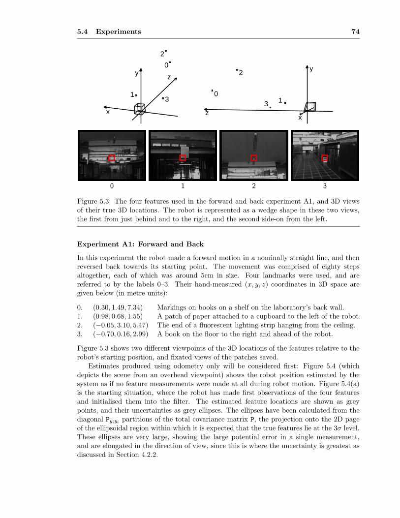
5.4 Experiments 74
z
x
13
y0
2
zx
y
13
2
0
0 1 2 3
Figure 5.3: The four features used in the forward and back experiment A1, and 3D viewsof their true 3D locations. The robot is represented as a wedge shape in these two views,the first from just behind and to the right, and the second side-on from the left.
Experiment A1: Forward and Back
In this experiment the robot made a forward motion in a nominally straight line, and thenreversed back towards its starting point. The movement was comprised of eighty stepsaltogether, each of which was around 5cm in size. Four landmarks were used, and arereferred to by the labels 0–3. Their hand-measured (x, y, z) coordinates in 3D space aregiven below (in metre units):
0. (0.30, 1.49, 7.34) Markings on books on a shelf on the laboratory’s back wall.1. (0.98, 0.68, 1.55) A patch of paper attached to a cupboard to the left of the robot.2. (−0.05, 3.10, 5.47) The end of a fluorescent lighting strip hanging from the ceiling.3. (−0.70, 0.16, 2.99) A book on the floor to the right and ahead of the robot.
Figure 5.3 shows two different viewpoints of the 3D locations of the features relative to therobot’s starting position, and fixated views of the patches saved.
Estimates produced using odometry only will be considered first: Figure 5.4 (whichdepicts the scene from an overhead viewpoint) shows the robot position estimated by thesystem as if no feature measurements were made at all during robot motion. Figure 5.4(a)is the starting situation, where the robot has made first observations of the four featuresand initialised them into the filter. The estimated feature locations are shown as greypoints, and their uncertainties as grey ellipses. The ellipses have been calculated from thediagonal Pyiyi
partitions of the total covariance matrix P, the projection onto the 2D pageof the ellipsoidal region within which it is expected that the true features lie at the 3σ level.These ellipses are very large, showing the large potential error in a single measurement,and are elongated in the direction of view, since this is where the uncertainty is greatest asdiscussed in Section 4.2.2.
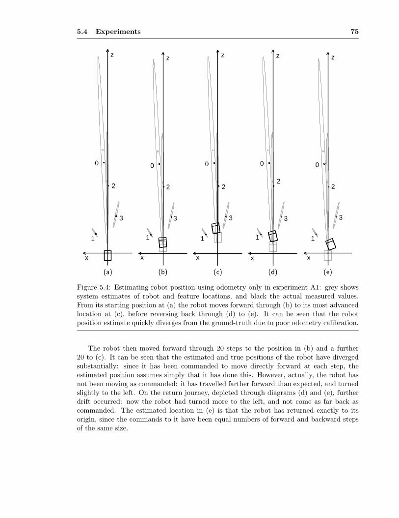
5.4 Experiments 75
x
1
3
2
z
0
x
1
3
0
2
z
x
1
3
z
2
0
x
1
2
3
0
z
x
1
3
2
0
z
(a) (b) (c) (d) (e)
Figure 5.4: Estimating robot position using odometry only in experiment A1: grey showssystem estimates of robot and feature locations, and black the actual measured values.From its starting position at (a) the robot moves forward through (b) to its most advancedlocation at (c), before reversing back through (d) to (e). It can be seen that the robotposition estimate quickly diverges from the ground-truth due to poor odometry calibration.
The robot then moved forward through 20 steps to the position in (b) and a further20 to (c). It can be seen that the estimated and true positions of the robot have divergedsubstantially: since it has been commanded to move directly forward at each step, theestimated position assumes simply that it has done this. However, actually, the robot hasnot been moving as commanded: it has travelled farther forward than expected, and turnedslightly to the left. On the return journey, depicted through diagrams (d) and (e), furtherdrift occurred: now the robot had turned more to the left, and not come as far back ascommanded. The estimated location in (e) is that the robot has returned exactly to itsorigin, since the commands to it have been equal numbers of forward and backward stepsof the same size.
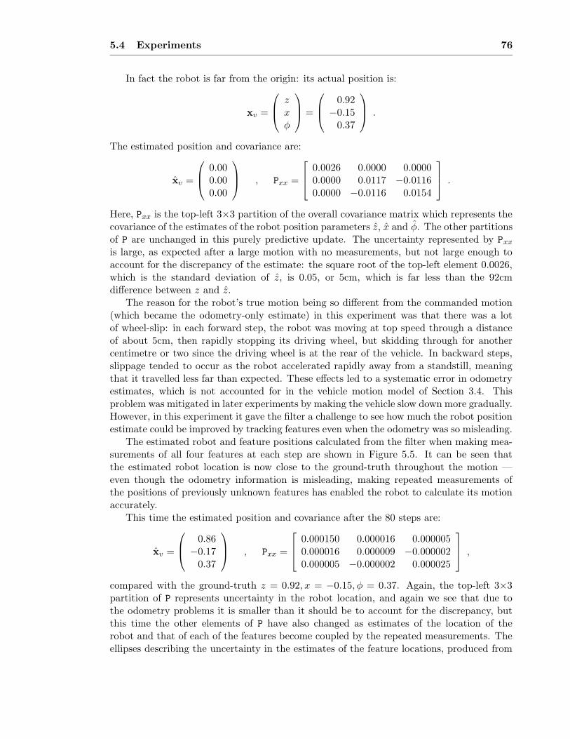
5.4 Experiments 76
In fact the robot is far from the origin: its actual position is:
xv =
zxφ
=
0.92−0.15
0.37
.
The estimated position and covariance are:
xv =
0.000.000.00
, Pxx =
0.0026 0.0000 0.00000.0000 0.0117 −0.01160.0000 −0.0116 0.0154
.
Here, Pxx is the top-left 3×3 partition of the overall covariance matrix which represents thecovariance of the estimates of the robot position parameters z, x and φ. The other partitionsof P are unchanged in this purely predictive update. The uncertainty represented by Pxx
is large, as expected after a large motion with no measurements, but not large enough toaccount for the discrepancy of the estimate: the square root of the top-left element 0.0026,which is the standard deviation of z, is 0.05, or 5cm, which is far less than the 92cmdifference between z and z.
The reason for the robot’s true motion being so different from the commanded motion(which became the odometry-only estimate) in this experiment was that there was a lotof wheel-slip: in each forward step, the robot was moving at top speed through a distanceof about 5cm, then rapidly stopping its driving wheel, but skidding through for anothercentimetre or two since the driving wheel is at the rear of the vehicle. In backward steps,slippage tended to occur as the robot accelerated rapidly away from a standstill, meaningthat it travelled less far than expected. These effects led to a systematic error in odometryestimates, which is not accounted for in the vehicle motion model of Section 3.4. Thisproblem was mitigated in later experiments by making the vehicle slow down more gradually.However, in this experiment it gave the filter a challenge to see how much the robot positionestimate could be improved by tracking features even when the odometry was so misleading.
The estimated robot and feature positions calculated from the filter when making mea-surements of all four features at each step are shown in Figure 5.5. It can be seen thatthe estimated robot location is now close to the ground-truth throughout the motion —even though the odometry information is misleading, making repeated measurements ofthe positions of previously unknown features has enabled the robot to calculate its motionaccurately.
This time the estimated position and covariance after the 80 steps are:
xv =
0.86−0.17
0.37
, Pxx =
0.000150 0.000016 0.0000050.000016 0.000009 −0.0000020.000005 −0.000002 0.000025
,
compared with the ground-truth z = 0.92, x = −0.15, φ = 0.37. Again, the top-left 3×3partition of P represents uncertainty in the robot location, and again we see that due tothe odometry problems it is smaller than it should be to account for the discrepancy, butthis time the other elements of P have also changed as estimates of the location of therobot and that of each of the features become coupled by the repeated measurements. Theellipses describing the uncertainty in the estimates of the feature locations, produced from
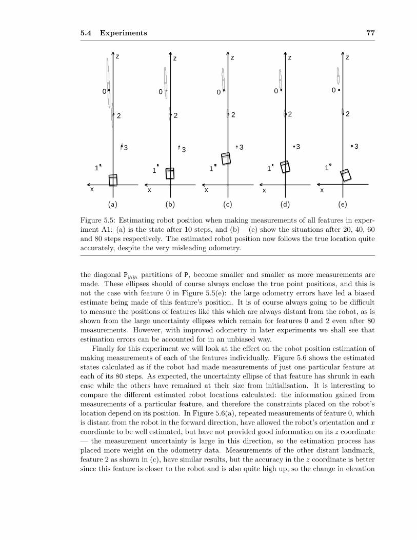
5.4 Experiments 77
2
0
x
3
z
1
x
1
0
z
2
3
x
1
0
z
2
3
x
1
0
z
2
3
x
1
0
z
2
3
(a) (b) (c) (d) (e)
Figure 5.5: Estimating robot position when making measurements of all features in exper-iment A1: (a) is the state after 10 steps, and (b) – (e) show the situations after 20, 40, 60and 80 steps respectively. The estimated robot position now follows the true location quiteaccurately, despite the very misleading odometry.
the diagonal Pyiyipartitions of P, become smaller and smaller as more measurements are
made. These ellipses should of course always enclose the true point positions, and this isnot the case with feature 0 in Figure 5.5(e): the large odometry errors have led a biasedestimate being made of this feature’s position. It is of course always going to be difficultto measure the positions of features like this which are always distant from the robot, as isshown from the large uncertainty ellipses which remain for features 0 and 2 even after 80measurements. However, with improved odometry in later experiments we shall see thatestimation errors can be accounted for in an unbiased way.
Finally for this experiment we will look at the effect on the robot position estimation ofmaking measurements of each of the features individually. Figure 5.6 shows the estimatedstates calculated as if the robot had made measurements of just one particular feature ateach of its 80 steps. As expected, the uncertainty ellipse of that feature has shrunk in eachcase while the others have remained at their size from initialisation. It is interesting tocompare the different estimated robot locations calculated: the information gained frommeasurements of a particular feature, and therefore the constraints placed on the robot’slocation depend on its position. In Figure 5.6(a), repeated measurements of feature 0, whichis distant from the robot in the forward direction, have allowed the robot’s orientation and xcoordinate to be well estimated, but have not provided good information on its z coordinate— the measurement uncertainty is large in this direction, so the estimation process hasplaced more weight on the odometry data. Measurements of the other distant landmark,feature 2 as shown in (c), have similar results, but the accuracy in the z coordinate is bettersince this feature is closer to the robot and is also quite high up, so the change in elevation

5.4 Experiments 78
x
1
3
2
0
z
x
1
0
2
3
z
x
1
0
2
3
z
x
1
0
2
3
z
(a) (b) (c) (d)
Figure 5.6: The estimated robot and feature locations in experiment A1 after 80 stepsmaking exclusive measurements of features 0, 1, 2 and 3 respectively in (a), (b), (c) and(d).
angle needed to fixate it will provide depth information as well as the change in vergence.Tracking feature 1 in (b), the closest feature to the robot, proves not to be very useful
in this experiment. The information that measurements of this feature are able to provideaccurately are the distance of the robot from it and the angle between the robot’s forwarddirection and viewing angle to the feature. Referring back to Figure 5.4(e), it can beenseen that final robot position calculated from the misleading odometry is in fact differentfrom the true position in such a way as to lie along the ambiguous degree of freedom ofthese measurements: that is to say, a measurement made of feature 1 from either the truerobot location or the estimated location would not differ much. The general nature of thisambiguity is made clearer in Figure 5.7. Measurements of feature 1 therefore do not helpto resolve the estimation error. Measuring feature 3, as in Figure 5.6(d), is much moreuseful, since its position means that it can help with the particular direction of error in thisexperiment.
The main observation to be drawn from this comparison is that it is necessary to makemeasurements of multiple features to fully constrain estimates of the robot’s motion. The

5.4 Experiments 79
Scene Feature
Figure 5.7: The different positions from which the robot will make the same measurementsof the pan, elevation and vergence angles to fixate on a feature lie along a circle. Thenecessary robot orientation is fixed relative to a point on this locus by the pan angle, sothere is only one degree of positional freedom. Measurements of the feature will not thereforereduce uncertainty along this direction.
estimates of Figure 5.5, where all the features have been measured, are much better thanany of the estimates produced from the features individually. This is a point which will bereturned to in Chapter 6 when the active choice of measurements is considered.
Experiment A2: Turning and Forward
In a second experiment, the robot made a turning, forward movement through a distance ofaround 2.5m while again making repeated measurements of four features. Figure 5.8 chartsthe progress of the estimation when measurements of all features were used, and comparesthis with the odometry-only estimate. It can be seen that the odometry information wasnow much more reliable (since wheel slippage had been reduced), and the robot positionestimate in (e) is quite close to the ground-truth. It can be seen from (d), however, thatthe estimate obtained when making measurements is much better still.
5.4.3 Experiment B: An Extended Run
In typical navigation, the robot will not solely make use of landmarks detected from itsstarting position as in the experiments above: prominent landmarks will be initialised,measured and sometimes rejected from the map at all stages of the journey. Chapter 7considers the automation of all these steps, but in this section an experiment is presentedwhere the robot moved through a long distance, building up and using a realistic map, andstopping at frequent step intervals so that ground-truth measurements of its position couldbe made. The key aim of the experiment was to verify the localisation algorithm over along run, and in particular check its ability to re-find features after long periods of neglectand “close the loop” on a round-trip journey.
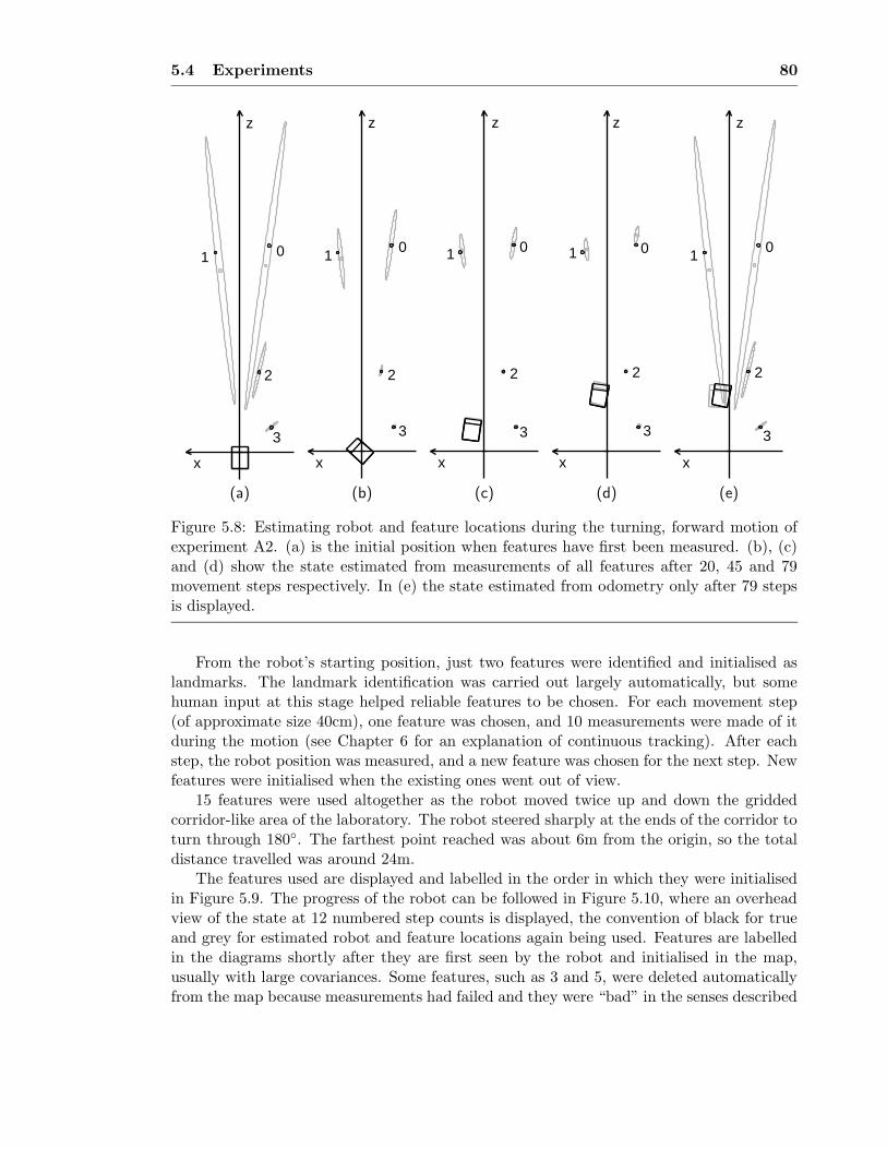
5.4 Experiments 80
x
3
2
1 0
z
x
3
2
10
z
x
3
2
1 0
z
x
3
2
1 0
z
x
3
2
10
z
(a) (b) (c) (d) (e)
Figure 5.8: Estimating robot and feature locations during the turning, forward motion ofexperiment A2. (a) is the initial position when features have first been measured. (b), (c)and (d) show the state estimated from measurements of all features after 20, 45 and 79movement steps respectively. In (e) the state estimated from odometry only after 79 stepsis displayed.
From the robot’s starting position, just two features were identified and initialised aslandmarks. The landmark identification was carried out largely automatically, but somehuman input at this stage helped reliable features to be chosen. For each movement step(of approximate size 40cm), one feature was chosen, and 10 measurements were made of itduring the motion (see Chapter 6 for an explanation of continuous tracking). After eachstep, the robot position was measured, and a new feature was chosen for the next step. Newfeatures were initialised when the existing ones went out of view.
15 features were used altogether as the robot moved twice up and down the griddedcorridor-like area of the laboratory. The robot steered sharply at the ends of the corridor toturn through 180◦. The farthest point reached was about 6m from the origin, so the totaldistance travelled was around 24m.
The features used are displayed and labelled in the order in which they were initialisedin Figure 5.9. The progress of the robot can be followed in Figure 5.10, where an overheadview of the state at 12 numbered step counts is displayed, the convention of black for trueand grey for estimated robot and feature locations again being used. Features are labelledin the diagrams shortly after they are first seen by the robot and initialised in the map,usually with large covariances. Some features, such as 3 and 5, were deleted automaticallyfrom the map because measurements had failed and they were “bad” in the senses described

5.4 Experiments 81
(0) (1) (2) (3) (4)
(5) (6) (7) (8) (9)
(10) (11) (12) (13) (14)
Figure 5.9: Fixated views of the 15 features used in the extended experiment B.
in Section 4.1. Feature 4 never shows up on the map because it was rejected very shortlyafter initialisation.
The robot moves up the corridor for the first time through steps (2), (7) and (10),before starting its first turn at step (14). It can be seen that the features initialised whenthe robot is at this end of the corridor, such as as numbers 5–9, have estimated positionswhich are much more uncertain than those initialised from near the origin such as 1 and2 — their uncertainty ellipses are quickly reduced to a size which is too small to show upon the diagrams. This reflects the fundamental characteristic of map building discussed inSection 5.2.1: these features are far (in terms of the number of measurements implicitlycompounded to estimate their locations) from the place where the coordinate frame isdefined; the robot location itself is uncertain when they are measured, and so their locationsare as well.
In step (22), the robot gets its first view of the back wall of the laboratory, and ini-tialises feature 10 which is the corner of a window. Step (27) is key, because it providesan opportunity to re-measure an early feature: number 2 comes back into view. The resultof this is that the estimate of the robot’s position immediately improves — it had beendrifting slightly up to step (22), but locks closely back on in (27). Also, the estimates ofthe locations of features initialised since measurements were last made of feature 2 improve,and their uncertainties reduce, due to their coupling to the robot state in the Kalman Filter— the uncertainty ellipses of features 6–9 and especially 10 visibly shrink. A further slightimprovement occurs in step (32) when feature 1 is re-found.
Close to the origin, the robot turns in step (35) and heads back up the corridor. Farfewer new features need to be initialised now because the old ones are visible from thispreviously-followed route. Turning again at the far end of the corridor in (53) and back atthe origin in (69), the robot halts at step (72), close to its starting position and orientation.
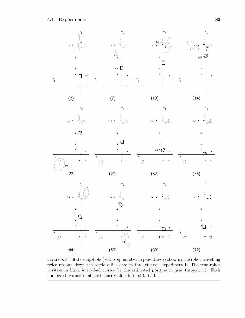
5.4 Experiments 82
x
1
z
0
x
2
3
z
5
6
z
x x
9
7
8
z
(2) (7) (10) (14)
z
x
10
x
z
x
11
z
x
z
(22) (27) (32) (35)
x
z12
x
13
z z
x
14
z
x
(44) (53) (69) (72)
Figure 5.10: State snapshots (with step number in parenthesis) showing the robot travellingtwice up and down the corridor-like area in the extended experiment B. The true robotposition in black is tracked closely by the estimated position in grey throughout. Eachnumbered feature is labelled shortly after it is initialised.

5.4 Experiments 83
The map of features generated sequentially through the experiment has now reached a fairlystable state, and there is no essential difference between landmarks detected early or latein the run.
To give a numerical idea of the localisation algorithm’s performance, at step (14), wherethe robot was starting to turn for the first time at the far end of the corridor, the true andestimated robot locations (in metre and radian units) were:
xv =
zxφ
=
5.17−0.15−0.39
, xv =
zx
φ
=
5.25−0.02−0.34
.
The covariance of the robot position estimate was:
Pxx =
0.0035 0.0003 0.00020.0003 0.0069 0.00330.0002 0.0033 0.0017
.
Feature 9, which had just been initialised here and had a large uncertainty, had true andestimated positions:
y9 =
X9
Y9
Z9
=
2.401.107.25
, y9 =
X9
Y9
Z9
=
2.801.047.29
,
and covariance
Py9y9=
0.1590 0.0186 0.09620.0186 0.0031 0.01610.0962 0.0161 0.1150
.
In each case, the large covariance accounted easily for the discrepancy within one or twostandard deviations: the robot’s x coordinate, for example, was incorrectly estimated by13cm, and the square root of the (2, 2) element of Pxx was
√0.0069 = 0.08: x had a standard
deviation of 8cm.We will also examine the later step (32), where the robot had returned to near the origin
and re-measured early features. Here the true and estimated robot locations were:
xv =
zxφ
=
0.780.312.76
, xv =
zx
φ
=
0.770.352.75
.
The covariance of the robot position estimate was:
Pxx =
0.00096 −0.00001 −0.00052−0.00001 0.00011 0.00002−0.00052 0.00002 0.00035
.
Feature 1, one of the features very close to the origin which was therefore known veryaccurately, had true and estimated positions:
y1 =
X1
Y1
Z1
=
−1.271.290.72
, y1 =
X1
Y1
Z1
=
−1.251.270.71
,

5.4 Experiments 84
Figure 5.11: (a) Artificial paper beacons in a straight horizontal line (spaced by 40cm). (b)The top-left corner of each paper patch was used as a feature.
and covariance
Py1y1=
0.00016 −0.00007 −0.00006−0.00007 0.00004 0.00004−0.00006 0.00004 0.00010
.
It can be seen that the estimates were very accurate: to within a few centimetres for boththe robot and feature positions. The covariances had shrunk to very small value, indeedslightly too small to account for the discrepancy between true and estimated values in avery small number of standard deviations (although in the case of feature 1, however, itmust be remembered that “ground truth” measurements of feature locations are somewhatapproximate). This indicates that the process or measurement noise in the filter mayhave been set too low, and the system had over-calculated its accuracy. However, systemperformance was not harmed, as can be seen from the algorithm’s continued success as therobot moved through subsequent steps.
5.4.4 Experiments C1 and C2: The Advantages of Carrying the FullCovariance Matrix
An experiment was set up to explicitly demonstrate the advantages of the full covariancemethod of map-building over using uncoupled filters for the generation of maps of featureswhich can be used for localisation over the equivalent of a “round trip” journey. As men-tioned earlier, uncoupled filter approaches fail here due to their inability to re-find featuresseen early in the run and form a globally consistent map. The coupled approach means thatautomatic re-registration with the original coordinate frame occurs when early features canbe measured again, as already demonstrated in the previous experiment.
An uncoupled-filters approach was easily implemented from our full-covariance systemby zeroing off-diagonal partitions of the large matrix P after every prediction and mea-surement update. It can be shown that this is equivalent to direct implementation of themost sensible uncoupled approach: the robot state xv and feature states yi are now indi-vidual entities, with covariances described only by the diagonal parts Pxx and Pyiyi
of the

5.4 Experiments 85
full covariance matrix. In a prediction, only the robot state and covariance change. In ameasurement update, only the state and covariance of the robot and the particular featureare affected; they become:
xv(k + 1|k + 1) = x(k + 1|k) + Pxx∂hi
∂xv
>
S−1ν (5.28)
Pxx(k + 1|k + 1) = Pxx(k + 1|k) − Pxx(k + 1|k)∂hi
∂xv
>
S−1 ∂hi
∂xvPxx(k + 1|k) (5.29)
yi(k + 1|k + 1) = yi(k + 1|k) + Pyiyi
∂hi
∂yi
>
S−1ν (5.30)
Pyiyi(k + 1|k + 1) = Pyiyi
(k + 1|k) − Pyiyi(k + 1|k)
∂hi
∂yi
>
S−1 ∂hi
∂yiPyiyi
(k + 1|k)(5.31)
S, the measurement variance (measurements still being split into their scalar components
as in Section 5.3.5), has a simpler form than in Equation 5.17:
S =∂hi
∂xvPxx
∂hi
∂xv
>
+∂hi
∂yiPyiyi
∂hi
∂yi
>
+ R . (5.32)
The effect of this S is that when performing updates of the robot state, the effective mea-surement uncertainty is the actual noise in the measurement plus the current uncertaintyin the feature’s position. When updating the estimate of the feature position, the effectivemeasurement uncertainty is the noise of the measurement plus the uncertainty in the robotposition. This is indeed the case, but what is not taken account of is possible coupling be-tween uncertainty in the robot and feature estimates: for example, the position of neithermay be known very well in the world coordinate frame, but the relative position is welldetermined. There is no way to represent this situation with uncoupled filters.
For the experiment, artificial beacons were created by affixing a row of paper markersto the bench at the side of the corridor (see Figure 5.11(a)). These beacons ensured thatthere was a regular supply of reliable features to measure along the forward and backwardrobot journeys. Also, the ground-truth locations of these landmarks could be measuredaccurately, and this made the coupled filter part of the experiment useful in itself becausethe accuracy of the system’s estimation of point positions could be investigated reliably.
Starting from the grid origin, the robot was driven forward in a nominally straight line.Every second paper feature was initialised and tracked for a short while on this outwardjourney, which was comprised of steps of around 40cm as in the previous experiment. Whenthe features were initialised by the robot, the selection of the original patch was donemanually to ensure that an exact part of each paper patch (in this case the top-left corneras shown in Figure 5.11(b)) was agreed on by robot and human ground-truth measurer. Therobot then reversed back down the corridor, tracking the features it had not previously seen.The aim was that it should return to its origin while tracking only recently acquired features,as would be the case in a looped movement around a rectangular layout of corridors forexample (such a layout was not available in our laboratory). Once the robot had returnedto near its starting position, it drove forward again, now attempting to re-measure featuresfound early on, completing the loop on the motion and establishing that a reliable maphad been formed. The whole experiment was carried out twice: once with the full coupledcovariance filter, and once with the uncoupled implementation.

5.4 Experiments 86
0
z
x
1
2
3
z
x
4
5
x
z
(0) (8) (13)
67
8
x
z
x
z
9
10
x
z
(19) (26) (27)
x
z
x
z
xy
z
(34) (34) Centred (34) Centred
Figure 5.12: Steps from experiment C1 using fully coupled robot and feature estimates.
Experiment C1: Carrying the Full Covariance Matrix
Results from the coupled run are displayed in Figure 5.12, labelled with step and featurenumbers. In the outward journey up to step (13), the robot position estimate starts to drift,its covariance grows, and the uncertainties in the positions of newly initialised features arelarge. This process continues as the robot returns to near the origin through steps (19)and (26) since only new features are tracked along the way. By now, the estimated robot
5.4 Experiments 87
location is quite offset from the ground-truth. Step (27) is the first after an initial feature isre-seen: measurements are made of feature 0. The robot estimate immediately locks backwell onto the true position. The estimate then remains good as the robot moves away fromthe origin again in step (34), now making measurements of other features.
The sign that the map-building has taken place consistently and without bias betweenfeatures detected early and late in the run is the pattern of the feature uncertainty ellipsesseen in steps (27) and (34): there is no distinction between the alternate ones measuredin the forward and backward runs. This is an impressive feat from the algorithm: havingreferences to well known features at both ends of the motion has allowed all the estimatesmade about features in between to be improved. What the pattern of uncertainty remaining,where uncertainty in the x direction grows in a regular way with distance from the origin,shows is the fundamental uncertainty in map-building from compounded measurements:because the features most distant from the origin can only be measured when the robot isat that end of the corridor (due to the limitations on range and angle in patch matchingdescribed in Section 4.1.2), estimates of their positions will be made uncertain due tothe implicit combination of a large number of successive measurements which goes intoestimating the robot’s position in this area.
It must be remembered though that the uncertainty in the farther features is only withrespect to the somewhat arbitrary global frame of reference defined at the robot’s startingposition: features 5 and 6 for instance, both have uncertainties which are large in the worldframe, but their position relative to one another is well known, this information being heldin the covariance partition Py5y6
. At step (34),
Py5y6=
0.01290 −0.00001 −0.000570.00000 0.00000 0.00000
−0.00052 0.00001 0.00034
.
The large value 0.01290 for the top-left element of this matrix partition shows that the Xcoordinates of these features are well correlated.
The correlation between features is demonstrated clearly in the last two pictures ofFigure 5.12 (the second a view from an angle as a reminder of the 3D nature of the map),where the state in step (34) is shown after the coordinate frame has been zeroed to therobot’s current position as in Section 5.3.8. It can be seen that those features currentlyclose to the robot, such as 3 and 8, are very well known in the new frame — their positionsrelative to the robot are certain because measurements need not be compounded to estimatethis. The features with the largest uncertainties in the new frame are those distant fromthe robot in both directions — there is nothing special about the original coordinate frame.
Experiment C2: Using Uncoupled Covariances
The experiment was re-run, now using uncoupled filters for the vehicle and feature statesas described above, but with similar robot actions. The state at various steps is shown inFigure 5.13. The state estimates seen in steps (7), (13) and (26) are similar in accuracyto those of experiment C1 — that is to say that the discrepancy between estimated robotand feature positions and ground truth is of around the same size. However, what hasnot happened correctly is growth in uncertainty in the robot state and that of the featuresinitialised late in the journey: the location of feature 10 at step (26), for instance, is clearly

5.5 Conclusion 88
x
z
0
12
3
x
z5
4
x
z
678
910
(7) (13) (26)
Figure 5.13: Steps from experiment C2 with uncoupled robot and feature estimates.
estimated quite incorrectly, but its uncertainty ellipse does not reflect this in the same wayas that of feature 10 in experiment C1 (Figure 5.12, step (26)).
Only 3 state pictures are shown in Figure 5.13, since the result of this misleading filteringwas that after step (26), the robot was unable to re-find the features found early-on, suchas feature 0. The uncoupled filter had led the robot to overconfidently estimate its locationwhen in fact there should have been a large uncertainty, and the feature did not lie in theimage search ellipses generated. The robot was therefore never able to re-register itself withthe original world frame as in experiment C1.
5.5 Conclusion
We have described an accurate and reliable approach to simultaneous map-building andlocalisation using active vision. The algorithm has been proven in experiments, and inparticular its ability to recognise features after periods of neglect to re-register with anoriginal coordinate frame is satisfying and essential to long-term navigation in confinedregions.

6Continuous Feature Tracking, andDeveloping a Strategy for Fixation
Active vision provides the capability to view and make measurements of features lyingover a wide range of viewpoints. The previous chapter has shown how it can be used ina localisation and map-building system using landmark features: in experiments, accurateinformation on a new absolute robot position could be obtained from measurements of oneor more of these features. However, we have not yet considered the strategy that shouldbe followed by the active cameras: we know how to extract all the information from aparticular measurement, but measurements of some features will be more valuable thanthose of others, or perhaps more convenient to obtain.
In particular, the active head allows the robot to track at fixation one feature in almostany viewing direction whenever the robot is moving, making repeated measurements of thatfeature as it does so which provide continuous navigation information. How this tracking isachieved will be considered in Section 6.1.
Maintaining a large map of features with full covariance storage, as described in the pre-vious chapter, presents computational difficulties to fast tracking of features with straight-forward full state updates at every step. In Section 6.2, a method is presented by whichcontinuous tracking is never compromised by the computational burden of maintaining alarge map, by updating in real-time only those parts of the state representation which areessential to the current tracking task. The effort to be expended at each step can be reducedto a constant amount. A small, constant amount of additional stored information allowsthe full state to be updated when the robot stops moving and has processing time to spare.
Section 6.3 considers the strategies that should be adopted to maximise the capabilitiesof the active head to make measurements of scene features and provide navigation informa-tion. Criteria based on the information content of measurements are developed to tackle

6.1 Continuous Tracking of Features 90
the questions of selecting between known features, selecting new features, and selecting be-tween features while the robot is moving. These will form an essential part of the automaticmap-building and localisation system to be presented in Chapter 7.
6.1 Continuous Tracking of Features
Tracking a feature consists of making repeated fixated measurements of it as the robotmoves past. This task is of course similar to that of tracking a moving target from astationary robot viewpoint, a problem which has been studied in depth already in activevision as described in Chapter 1. The situation is somewhat simplified, however, when therelative movement between robot and target is provided by the robot: the robot is under itsown control, so its motion is at least approximately known. Tracking a freely manoeuvringtarget is difficult because although a model of its possible motions may be known, the“control inputs” are not. This is not the case when a robot tracks a stationary target.
Also, in the robot vehicle motion model of Section 3.4, it was shown that movementscould be described directly in terms of the two control inputs velocity and steering angle —knowledge of these allows an estimate of a new position to be calculated from the previousposition estimate without extra parameters. This might not be the case in a robot withmore complex dynamics: suppose it was like a normal road car, where the control inputs arethe steering angle and the position of the accelerator pedal, which is more closely related tothe acceleration of the vehicle than its actual speed (as discussed by Maybank et al. [59] withregard to visual tracking of externally viewed cars) — in order to produce a new positionestimate, it is necessary to know the current velocity as well as the current position. Thevelocity must therefore be part of the state vector of estimated quantities. Other vehiclesmay require higher-order derivatives to be estimated as well.
For these reasons, our tracking algorithm can proceed quasi-statically. This meansthat continuous tracking can be performed with the same filtering approach as would beused if the robot was moving in a step-by-step fashion, stopping each time a measurementwas to be made. Assuming a certain inter-measurement interval, as the robot starts amovement, the prediction step of the filter produces an estimate of its new position atthe next measurement point, and the expected relative position of the target feature iscalculated. The active head is then driven to fixate on where the feature should be found,and the robot waits to make its measurement as the interval checkpoint on its trajectoryis passed. As mentioned in Section 2.7, the vehicle odometry is used as the trigger formeasurements: the trajectory is divided into steps of equal numbers of wheel encodercounts. This is better than using strict time intervals, since the distance travelled is whatreally matters, and possible fluctuations in velocity (particularly when the robot is juststarting or stopping) will be unimportant. Because of this, the measurement frequency isnot strictly constant, but in current implementation tracking is performed at approximately5Hz (the odometry measurement intervals being dynamically set proportional to the robotvelocity to keep this constant).
The actions taken in a step of the tracking loop, during which the robot drives contin-uously, are therefore:
1. Based on the current control inputs, perform the prediction step of the filter andestimate the new robot position.

6.2 Updating Motion and Structure Estimates in Real Time 91
Figure 6.1: Image sequences obtained from continuous fixation tracking of features.
2. Calculate the estimated head angles for fixation on the feature, and move the head tothis position in readiness.
3. Wait until the robot has reached the correct “new” position according to its odometry.
4. Obtain new images from the cameras.
5. Perform correlation searching for the feature as in Section 4.1.2.
6. If the feature is found in both images, perform a measurement update of the filter.
Figure 6.1 shows image sequences obtained from one of the robot’s cameras in periods offixation tracking.
6.2 Updating Motion and Structure Estimates in Real Time
As explained in Chapter 5, when estimating multiple quantities in a Kalman Filter frame-work (in our case the positions of the robot and the features it uses as landmarks) , the bestapproach is to combine the estimates into a single state vector and to store the uncertaintyin the estimates in an overall covariance matrix. However, a problem with proceeding inthis way is that once the number of quantities being estimated becomes large (in our casethe number of landmarks), the sizes of the state vector and in particular the covariancematrix make them unwieldy and computationally expensive to update at each step of thefilter’s evolution. This will clearly present a problem to a system with limited processingresources attempting to run at a high update rate, as with our robot when continuouslytracking a feature while moving.
In this section we present an approach which under certain common circumstances willreduce the computation to be performed per time-step to a constant small amount so thatreal-time operation can be achieved regardless of the size of the state vector. The key tothe method is to update only the parts of the state vector and covariance matrix whichare necessary to the current real-time operation. Information about the generic way toupdate the other parts of the vector and matrix is stored at the same time (requiring a

6.2 Updating Motion and Structure Estimates in Real Time 92
small and constant amount of computation and storage) so that these parts can be fullyupdated at the end of the real-time run. The method is not an approximation, but asimple re-arrangement of the book-keeping of updating the estimates. The method will bepresented in a formulation as general as possible to demonstrate its potential applicationto other map-building and localisation systems. Some of the notation and derivations fromChapter 5 will be re-stated in this general form for clarity. A summary of the details neededfor implementation is given in Section 6.2.5.
6.2.1 Situation and Notation
We consider the general situation of estimating the locations of a moving sensor and severalstationary features of which it is able to make measurements. The state of the system canbe represented by the stacked vector
x =
xv
y1
y2...
, (6.1)
where xv is the location (or more generally the state) of the sensor, and yi is the locationof the ith feature.
Our current estimate of this true state is the vector x with covariance matrix P. Thesecan be written in the partitioned forms:
x =
xv
y1
y2...
, P =
Pxx Pxy1Pxy2
. . .Py1x Py1y1
Py1y2. . .
Py2x Py2y1Py2y2
. . ....
......
. (6.2)
The partitioned sections of the covariance matrix represent the coupling of the uncertaintiesin the different parts of the estimated state. Pxyi
is the covariance matrix between theestimated robot state xv and that of one of the features yi, while Pyiyj
is that between theestimated locations of two features yi and yj .
Recalling the standard Extended Kalman Filter prediction and update formulae fromSection 5.1, we impose the simplifying specifics of the situation under consideration. Theseare:
1. The state transition function f has the form
f(x) =
fv(xv,u)y1
y2...
. (6.3)
This means simply that only the sensor moves in the scene, and not the features.Function fv models the sensor movement — u is the control vector which may ormay not be known depending on the exact scenario. The yi feature parts of the statevector do not change in the state transition.
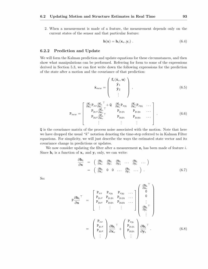
6.2 Updating Motion and Structure Estimates in Real Time 93
2. When a measurement is made of a feature, the measurement depends only on thecurrent states of the sensor and that particular feature:
h(x) = hi(xv,yi) . (6.4)
6.2.2 Prediction and Update
We will form the Kalman prediction and update equations for these circumstances, and thenshow what manipulations can be performed. Referring for form to some of the expressionsderived in Section 5.3, we can first write down the following expressions for the predictionof the state after a motion and the covariance of that prediction:
xnew =
fv(xv,u)y1
y2...
, (6.5)
Pnew =
∂fv∂xv
Pxx∂fv∂xv
>+ Q
∂fv∂xv
Pxy1
∂fv∂xv
Pxy2. . .
Py1x∂fv∂xv
>Py1y1
Py1y2. . .
Py2x∂fv∂xv
>Py2y1
Py2y2. . .
......
...
. (6.6)
Q is the covariance matrix of the process noise associated with the motion. Note that herewe have dropped the usual “k” notation denoting the time-step referred to in Kalman Filterequations. For simplicity, we will just describe the ways the estimated state vector and itscovariance change in predictions or updates.
We now consider updating the filter after a measurement zi has been made of feature i.Since hi is a function of xv and yi only, we can write:
∂hi
∂x=
(
∂hi
∂xv
∂hi
∂y1
∂hi
∂y2. . . ∂hi
∂yi. . .
)
=(
∂hi
∂xv0 0 . . . ∂hi
∂yi. . .
)
. (6.7)
So:
P∂hi
∂x
>
=
Pxx Pxy1Pxy2
. . .Py1x Py1y1
Py1y2. . .
Py2x Py2y1Py2y2
. . ....
......
∂hi
∂xv
>
0
0
...∂hi
∂yi
>
...
=
Pxx
Py1x
Py2x
...
∂hi
∂xv
>
+
Pxyi
Py1yi
Py2yi
...
∂hi
∂yi
>
. (6.8)
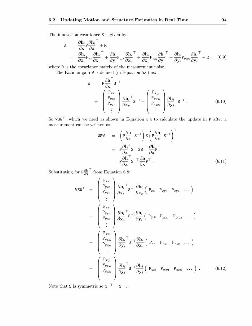
6.2 Updating Motion and Structure Estimates in Real Time 94
The innovation covariance S is given by:
S =∂hi
∂xP∂hi
∂x
>
+ R
=∂hi
∂xvPxx
∂hi
∂xv
>
+∂hi
∂yiPyix
∂hi
∂xv
>
+∂hi
∂xvPxyi
∂hi
∂yi
>
+∂hi
∂yiPyiyi
∂hi
∂yi
>
+ R , (6.9)
where R is the covariance matrix of the measurement noise.The Kalman gain W is defined (in Equation 5.6) as:
W = P∂h
∂x
>
S−1
=
Pxx
Py1x
Py2x
...
∂hi
∂xv
>
S−1 +
Pxyi
Py1yi
Py2yi
...
∂hi
∂yi
>
S−1 . (6.10)
So WSW>, which we need as shown in Equation 5.4 to calculate the update in P after ameasurement can be written as
WSW> =
(
P∂h
∂x
>
S−1
)
S
(
P∂h
∂x
>
S−1
)>
= P∂h
∂x
>
S−1SS
−>∂h
∂xP>
= P∂h
∂x
>
S−>∂h
∂xP> . (6.11)
Substituting for P∂h∂x
>from Equation 6.8:
WSW> =
Pxx
Py1x
Py2x
...
∂hi
∂xv
>
S−1 ∂hi
∂xv
(
Pxx Pxy1Pxy2
. . .)
+
Pxx
Py1x
Py2x
...
∂hi
∂xv
>
S−1 ∂hi
∂yi
(
Pyix Pyiy1Pyiy2
. . .)
+
Pxyi
Py1yi
Py2yi
...
∂hi
∂yi
>
S−1 ∂hi
∂xv
(
Pxx Pxy1Pxy2
. . .)
+
Pxyi
Py1yi
Py2yi
...
∂hi
∂yi
>
S−1 ∂hi
∂yi
(
Pyix Pyiy1Pyiy2
. . .)
. (6.12)
Note that S is symmetric so S−> = S−1.
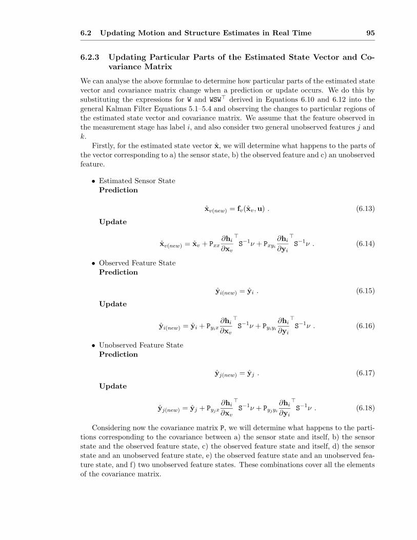
6.2 Updating Motion and Structure Estimates in Real Time 95
6.2.3 Updating Particular Parts of the Estimated State Vector and Co-variance Matrix
We can analyse the above formulae to determine how particular parts of the estimated statevector and covariance matrix change when a prediction or update occurs. We do this bysubstituting the expressions for W and WSW> derived in Equations 6.10 and 6.12 into thegeneral Kalman Filter Equations 5.1–5.4 and observing the changes to particular regions ofthe estimated state vector and covariance matrix. We assume that the feature observed inthe measurement stage has label i, and also consider two general unobserved features j andk.
Firstly, for the estimated state vector x, we will determine what happens to the parts ofthe vector corresponding to a) the sensor state, b) the observed feature and c) an unobservedfeature.
• Estimated Sensor StatePrediction
xv(new) = fv(xv,u) . (6.13)
Update
xv(new) = xv + Pxx∂hi
∂xv
>
S−1ν + Pxyi
∂hi
∂yi
>
S−1ν . (6.14)
• Observed Feature StatePrediction
yi(new) = yi . (6.15)
Update
yi(new) = yi + Pyix∂hi
∂xv
>
S−1ν + Pyiyi
∂hi
∂yi
>
S−1ν . (6.16)
• Unobserved Feature StatePrediction
yj(new) = yj . (6.17)
Update
yj(new) = yj + Pyjx∂hi
∂xv
>
S−1ν + Pyjyi
∂hi
∂yi
>
S−1ν . (6.18)
Considering now the covariance matrix P, we will determine what happens to the parti-tions corresponding to the covariance between a) the sensor state and itself, b) the sensorstate and the observed feature state, c) the observed feature state and itself, d) the sensorstate and an unobserved feature state, e) the observed feature state and an unobserved fea-ture state, and f) two unobserved feature states. These combinations cover all the elementsof the covariance matrix.

6.2 Updating Motion and Structure Estimates in Real Time 96
To simplify the following expressions we define these matrices:
A =∂hi
∂xv
>
S−1 ∂hi
∂xv(6.19)
B =∂hi
∂xv
>
S−1 ∂hi
∂yi(6.20)
C =∂hi
∂yi
>
S−1 ∂hi
∂xv(6.21)
D =∂hi
∂yi
>
S−1 ∂hi
∂yi(6.22)
• Covariance between Sensor State and ItselfPrediction
Pxx(new) =∂fv∂xv
Pxx∂fv∂xv
>
+ Q . (6.23)
Update
Pxx(new) = Pxx − (PxxAPxx + PxxBPyix + PxyiCPxx + Pxyi
DPyix) . (6.24)
• Covariance between Sensor State and Observed Feature StatePrediction
Pxyi(new) =∂fv∂xv
Pxyi. (6.25)
Update
Pxyi(new) = Pxyi− (PxxAPxyi
+ PxxBPyiyi+ Pxyi
CPxyi+ Pxyi
DPyiyi) . (6.26)
• Covariance between Observed Feature State and ItselfPrediction
Pyiyi(new) = Pyiyi. (6.27)
Update
Pyiyi(new) = Pyiyi− (PyixAPxyi
+ PyixBPyiyi+ Pyiyi
CPxyi+ Pyiyi
DPyiyi) . (6.28)
• Covariance between Sensor State and an Unobserved Feature StatePrediction
Pxyj(new) =∂fv∂xv
Pxyj. (6.29)
Update
Pxyj(new) = Pxyj−(
PxxAPxyj+ PxxBPyiyj
+ PxyiCPxyj
+ PxyiDPyiyj
)
. (6.30)

6.2 Updating Motion and Structure Estimates in Real Time 97
• Covariance between Observed Feature State and an Unobserved Feature StatePrediction
Pyiyj(new) = Pyiyj. (6.31)
Update
Pyiyj(new) = Pyiyj−(
PyixAPxyj+ PyixBPyiyj
+ PyiyiCPxyj
+ PyiyiDPyiyj
)
. (6.32)
• Covariance between Two Unobserved Feature StatesPrediction
Pyjyk(new) = Pyjyk. (6.33)
Update
Pyjyk(new) = Pyjyk−(
PyjxAPxyk+ PyjxBPyiyk
+ PyjyiCPxyk
+ PyjyiDPyiyk
)
. (6.34)
Note that this last expression also covers the case where j = k, where it is thecovariance between an unobserved feature state and itself.
6.2.4 Multiple Steps
The form of the expressions above allows efficient filtering to be performed in the casewhere a single feature is observed exclusively over multiple time steps. This of course occursfrequently in the active navigation system described in this thesis where single features aretracked for extended periods.
Let the estimated state vector and covariance at the start of a motion where a singlefeature i is to be tracked be:
x(0) =
xv(0)y1(0)y2(0)
...
, P(0) =
Pxx(0) Pxy1(0) Pxy2
(0) . . .Py1x(0) Py1y1
(0) Py1y2(0) . . .
Py2x(0) Py2y1(0) Py2y2
(0) . . ....
......
. (6.35)
During the extended period of measurements of one feature, Equations 6.13–6.16 and 6.23–6.28 show that it will be necessary to update the parts of the state vector and covariancematrix which are directly involved in the tracking process at all times: these are the esti-mated states of the sensor and observed feature, xv and yi, and the covariance elements Pxx,Pxyi
and Pyiyi. However, it will not be essential to update the other parts of the estimated
state vector and covariance matrix at every step: they play no part in the updates of thequantities just mentioned. We will show how a small amount of information can be storedat each filter step which allows the other sections of the state and covariance to be updatedin a generic way at the end of the tracking motion.
• Pxyjand Pyiyj

6.2 Updating Motion and Structure Estimates in Real Time 98
We look first at the parts Pxyjand Pyiyj
of the covariance matrix: the forms of theirprediction and update changes given in Equations 6.29–6.32 suggest that it is possiblealways to express them in the form
Pxyj= ETPxyj
(0) + FTPyiyj(0) (6.36)
Pyiyj= GTPyiyj
(0) + HTPxyj(0) , (6.37)
where ET , FT , GT and HT are as yet undetermined matrices. To find how these ma-trices evolve over time, we consider first a single measurement update. From Equa-tions 6.30 and 6.32:
Pxyj(new) = Pxyj− [PxxA + Pxyi
C] Pxyj− [PxxB + Pxyi
D] Pyiyj, (6.38)
Pyiyj(new) = Pyiyj− [PyixA + Pyiyi
C] Pxyj− [PyixB + Pyiyi
D] Pyiyj. (6.39)
(6.40)
We define the matrices E, F, G and H as:
E = I− [PxxA + PxyiC] (6.41)
F = − [PxxB + PxyiD] (6.42)
G = I− [PyixB + PyiyiD] (6.43)
H = − [PyixA + PyiyiC] (6.44)
So:
Pxyj(new) = EPxyj+ FPyiyj
, (6.45)
Pyiyj(new) = GPyiyj+ HPxyj
. (6.46)
Therefore, recalling the form in which we would like to express Pxyjand Pyiyj
given inEquations 6.36 and 6.37, the coefficient matrices ET , FT , GT and HT should be alteredas follows:
ET (new) = EET + FHT (6.47)
FT (new) = EFT + FGT (6.48)
GT (new) = GGT + HFT (6.49)
HT (new) = GHT + HET (6.50)
in a measurement update.
Altering ET , FT , GT and HT at a prediction is much easier: Equations 6.29 and 6.31tell us that:
ET (new) =∂fv∂xv
ET , (6.51)
FT (new) =∂fv∂xv
FT . (6.52)
GT and HT are unchanged.

6.2 Updating Motion and Structure Estimates in Real Time 99
• Pyjyk
With this part of the covariance matrix, the covariance between the position esti-mate of two of the unobserved features, the prediction and measurement updates inEquations 6.33 and 6.34 suggest that we can express it in the form:
Pyjyk= Pyjyk
(0) − [ Pyjx(0)ATPxyk(0)
+ Pyjx(0)BTPyiyk(0)
+ Pyjyi(0)CTPxyk
(0)
+ Pyjyi(0)DTPyiyk
(0) ] . (6.53)
From Equation 6.34 we can write down the form of a single measurement update:
Pyjyk(new) = Pyjyk− [PyjxAPxyk
+ PyjxBPyiyk+ Pyjyi
CPxyk+ Pyjyi
DPyiyk] (6.54)
Substituting in for Pxyj, Pyiyj
, Pxykand Pyiyk
(and their transposes) from the expres-sions found in the previous section (Equations 6.36 and 6.37) and rearranging, weobtain:
Pyjyk(new) = Pyjyk
− Pyjx(0)[E>T AET + E>T BHT + H
>T CET + H
>T DHT ]Pxyk
(0)
− Pyjx(0)[E>T AFT + E>T BGT + H
>T CFT + H
>T DGT ]Pyiyk
(0)
− Pyjyi(0)[F>T AET + F
>T BHT + G
>T CET + G
>T DHT ]Pxyk
(0)
− Pyjyi(0)[F>T AFT + F
>T BGT + G
>T CFT + G
>T DGT ]Pyiyk
(0) (6.55)
We can therefore deduce the way in which the coefficient matrices AT , BT , CT and DT
should be altered at a measurement update:
AT (new) = AT + E>T AET + E
>T BHT + H
>T CET + H
>T DHT (6.56)
BT (new) = BT + E>T AFT + E
>T BGT + H
>T CFT + H
>T DGT (6.57)
CT (new) = CT + F>T AET + F
>T BHT + G
>T CET + G
>T DHT (6.58)
DT (new) = DT + F>T AFT + F
>T BGT + G
>T CFT + G
>T DGT (6.59)
Since Equation 6.33 shows that Pyjykis unchanged in a prediction, it is not necessary
to change AT , BT , CT and DT when a prediction occurs.
• yj
With the estimated state yj of an unobserved feature, looking at Equations 6.17and 6.18 suggests that we can write it as
yj = yj(0) + Pyjx(0)mT + Pyjyi(0)nT , (6.60)
where mT and nT are vectors whose form is to be determined.
From Equation 6.18, the form of a measurement update is
yj(new) = yj + Pyjx∂hi
∂xv
>
S−1ν + Pyjyi
∂hi
∂yi
>
S−1ν . (6.61)

6.2 Updating Motion and Structure Estimates in Real Time 100
We substitute in the expressions for Pyjx and Pyjyifrom Equations 6.36 and 6.37 to
obtain:
yj(new) = yj
+Pyjx(0)
(
E>T
∂hi
∂xv
>
+ H>T
∂hi
∂yi
>)
S−1ν
+Pyjyi(0)
(
F>T
∂hi
∂xv
>
+ G>T
∂hi
∂yi
>)
S−1ν
(6.62)
Therefore, in a measurement step we alter mT and nT as follows:
mT (new) = mT +
(
E>T
∂hi
∂xv
>
+ H>T
∂hi
∂yi
>)
S−1ν (6.63)
nT (new) = nT +
(
F>T
∂hi
∂xv
>
+ G>T
∂hi
∂yi
>)
S−1ν (6.64)
In a prediction step, Equation 6.17 shows that we do not need to alter mT and nT
because yj does not change.
6.2.5 Summary
For clarity, we summarise the method described above. The situation under considera-tion is that of a sensor moving amongst multiple features of interest, but currently makingmeasurements of only one, labelled i. The labels j and k describe two general unobservedfeatures. The method describes the way in which, while the parts of the estimated statevector and covariance matrix which are directly involved in the motion and measurementsare continuously updated, the information about how generically to update the other sec-tions can be efficiently stored so that a single step can bring them up to date at the end ofthe motion.
At the start of the motion, the estimated state vector and covariance of the systemare denoted by x(0) and P(0). The following matrices and vectors, which will store thegeneric update information (the T subscript being coined with the word “total” in mind),are initialised as follows:
AT = 0
BT = 0
CT = 0
DT = 0
ET = I
FT = 0
GT = I
HT = 0
mT = 0
nT = 0 (6.65)
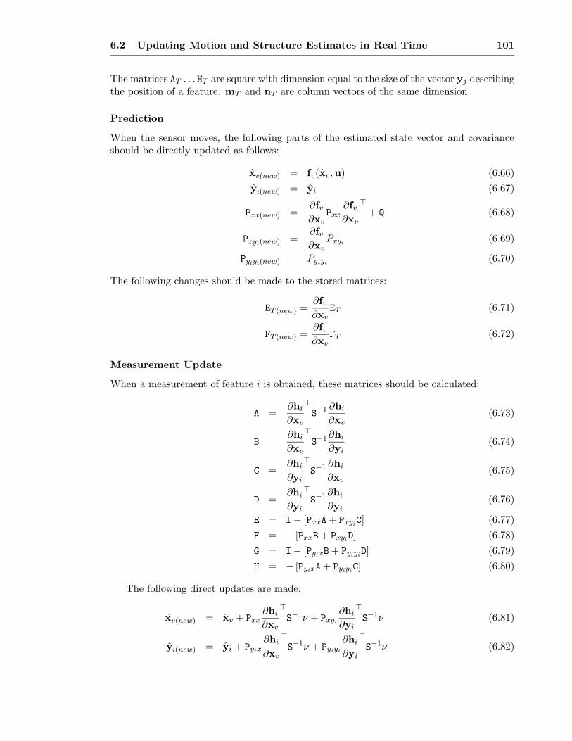
6.2 Updating Motion and Structure Estimates in Real Time 101
The matrices AT . . . HT are square with dimension equal to the size of the vector yj describingthe position of a feature. mT and nT are column vectors of the same dimension.
Prediction
When the sensor moves, the following parts of the estimated state vector and covarianceshould be directly updated as follows:
xv(new) = fv(xv,u) (6.66)
yi(new) = yi (6.67)
Pxx(new) =∂fv∂xv
Pxx∂fv∂xv
>
+ Q (6.68)
Pxyi(new) =∂fv∂xv
Pxyi(6.69)
Pyiyi(new) = Pyiyi(6.70)
The following changes should be made to the stored matrices:
ET (new) =∂fv∂xv
ET (6.71)
FT (new) =∂fv∂xv
FT (6.72)
Measurement Update
When a measurement of feature i is obtained, these matrices should be calculated:
A =∂hi
∂xv
>
S−1 ∂hi
∂xv(6.73)
B =∂hi
∂xv
>
S−1 ∂hi
∂yi(6.74)
C =∂hi
∂yi
>
S−1 ∂hi
∂xv(6.75)
D =∂hi
∂yi
>
S−1 ∂hi
∂yi(6.76)
E = I− [PxxA + PxyiC] (6.77)
F = − [PxxB + PxyiD] (6.78)
G = I− [PyixB + PyiyiD] (6.79)
H = − [PyixA + PyiyiC] (6.80)
The following direct updates are made:
xv(new) = xv + Pxx∂hi
∂xv
>
S−1ν + Pxyi
∂hi
∂yi
>
S−1ν (6.81)
yi(new) = yi + Pyix∂hi
∂xv
>
S−1ν + Pyiyi
∂hi
∂yi
>
S−1ν (6.82)

6.2 Updating Motion and Structure Estimates in Real Time 102
Pxx(new) = Pxx − (PxxAPxx + PxxBPyix + PxyiCPxx + Pxyi
DPyix) (6.83)
Pxyi(new) = Pxyi− (PxxAPxyi
+ PxxBPyiyi+ Pxyi
CPxyi+ Pxyi
DPyiyi) (6.84)
Pyiyi(new) = Pyiyi− (PyixAPxyi
+ PyixBPyiyi+ Pyiyi
CPxyi+ Pyiyi
DPyiyi) (6.85)
These changes are then made to the stored matrices and vectors:
mT (new) = mT +
(
E>T
∂hi
∂xv
>
+ H>T
∂hi
∂yi
>)
S−1ν (6.86)
nT (new) = nT +
(
F>T
∂hi
∂xv
>
+ G>T
∂hi
∂yi
>)
S−1ν (6.87)
AT (new) = AT + E>T AET + E
>T BHT + H
>T CET + H
>T DHT (6.88)
BT (new) = BT + E>T AFT + E
>T BGT + H
>T CFT + H
>T DGT (6.89)
CT (new) = CT + F>T AET + F
>T BHT + G
>T CET + G
>T DHT (6.90)
DT (new) = DT + F>T AFT + F
>T BGT + G
>T CFT + G
>T DGT (6.91)
ET (new) = EET + FHT (6.92)
FT (new) = EFT + FGT (6.93)
GT (new) = GGT + HFT (6.94)
HT (new) = GHT + HET (6.95)
Note that the order of these changes is important because the expressions updating mT ,nT and AT . . . DT make use of the old values of ET . . . HT . When performing the updates ofET . . . HT in Equations 6.92 – 6.95, the matrices on the right hand side of the expressionsalways refer to the old versions of ET . . . HT , so care must be taken here and some temporarystorage used.
So the computational expense involved in making updates to the stored matrices andvectors at a prediction or measurement is constant, independent of the number of features inthe map. We store just information on the generic way in which the currently unimportantparts of the total state vector and covariance matrix can later be brought up to date.
Final Full Update
At the end of the motion, the whole estimated state vector can be brought up to date usingthe following expression for each unobserved feature j:
yj = yj(0) + Pyjx(0)mT + Pyjyi(0)nT . (6.96)
This expression describes how to update the covariance between a pair of unobserved fea-tures j and k:
Pyjyk= Pyjyk
(0) − [ Pyjx(0)ATPxyk(0)
+ Pyjx(0)BTPyiyk(0)
+ Pyjyi(0)CTPxyk
(0)
+ Pyjyi(0)DTPyiyk
(0) ] . (6.97)

6.3 A Strategy for Fixation: Selecting Which Feature to Track 103
Finally, the parts of the covariance matrix relating unobserved feature j to the sensor stateand observed feature state can be brought up to date as follows:
Pxyj= ETPxyj
(0) + FTPyiyj(0) , (6.98)
Pyiyj= GTPyiyj
(0) + HTPxyj(0) . (6.99)
Note that the order of operation is again important here, since it is necessary that Pxyj,
Pyiyj, Pxyk
and Pyiykremain at their initial (0) values for the update of the Pyjyk
matrixelement.
This final update stage has a computational complexity which is proportional to thesquare of the number of features in the map.
6.3 A Strategy for Fixation: Selecting Which Feature toTrack
The previous two sections have shown how it is possible to track a feature while the robot ismoving to give continuous information on the robot and feature positions. The active headallows tracked features to lie within a very wide field of view, meaning that the same one canbe tracked as the robot makes large movements, or alternatively that a variety of differentfeatures can be tracked at different stages of a motion. The fact that choice is availablemeans that a strategy for selecting features to be observed is required. As discussed inSection 4.1.2, only a subset of features in the map will be viewable from a certain robotlocation, due to constraints of viewing direction and distance, but which should be observedat a given time? Also, when is it time to look for new landmarks, and is it sensible to lookfor them in a particular place?
First, it is necessary to consider in which senses one feature could be “better” thananother to make measurements from:
• If measurements of that feature would provide more useful information.
• If less effort is required to make the measurements.
That some measurements can be more valuable than others in terms of informationcontent is quickly apparent: depending on which components of the current estimatedquantities, in particular the robot’s estimated position coordinates z, x and φ, are currentlythe least certain, it will be more useful to make measurements of features lying in certainpositions. If for instance the robot’s location is uncertain primarily in the forward/backwarddirection, there will be little use in making a measurement of a feature which lies directlyahead at a large range, since the large depth uncertainty of this measurement would providelittle extra constraint on the robot position.
The factor of the “effort” needed to make a measurement comes into effect when severalmeasurements are being strung together in a certain time interval: time spent moving toobserve or searching for one feature could alternatively be used to measure another one.The most clear example is if one feature is currently being tracked at fixation, but there isthe possibility of making a saccade to observe another feature while the robot keeps moving:making that potentially large head movement will be costly compared to making the smalladjustment to stay fixated on the current feature, so we would expect the information quality

6.3 A Strategy for Fixation: Selecting Which Feature to Track 104
of the alternative feature to have to be greater than that of the current by a reasonableamount to make the saccade worthwhile. This is the question which will be addressed inSection 6.3.3.
Active fixation switching is very evident in human and animal navigation — the humaneye is rarely at rest as it rapidly shifts between points of interest. During a period of walking,for example, attention will be divided between the ground surface, obstacles, near and farlandmarks and other objects of interest. Blind navigation is unreliable and dangerous, as iseasily demonstrated by the discomfort felt during an attempt at walking with closed eyes:the urge to re-open the eyes and reorient is very strong. Further, though, staring at justone feature in the world for an extended period while moving can be disorientating — it isnecessary to pay attention to a variety of landmarks to be fully confident of safe navigation.Investigating feature selection in this section casts some light on these natural behavioursas well as providing a key part of the robot navigation system, where the full statisticalinformation stored about the estimates of robot and feature positions means that we are ina position to make reasoned decisions about which features to measure at a given time.
6.3.1 Choosing from Known Features
We will first consider making a choice between known and currently visible features for animmediate measurement. Because it is intended for long-term use, what is important in themap-building system is the integrity and consistency of the whole map and the estimate ofthe robot’s position within it. We aim to maximise this with our choice of feature, ratherthan specifically the estimate of the robot position or that of the chosen feature — theseare quantities which live in the world coordinate frame, which is arbitrarily chosen. Therelative locations of robot and features are what matter for navigation. Furthermore, theseestimates are all intricately coupled by previous measurements — it would be somewhatmeaningless to try to optimise just a subset of them. However, we will see below thatchoice of feature on this basis usually does provide the best improvement in the explicitworld-frame estimate of the robot location.
The basis of the approach used is to make a measurement where the ability to predictis lowest, as discussed and derived in recent work by Whaite and Ferrie [100] in their paperabout active exploration to determine the shapes of surfaces. Speaking generally, given achoice of measurements in a system where the uncertainty in estimates of the parameters ofinterest is known, it makes sense to make the one where we are least certain of the result,since this will in a sense “squash” the total uncertainty, viewed as a multi-dimensionalellipsoid, along the longest axis available. If there is any part of the estimated state vectorwhich is particularly poorly known, this choice of measurement will act to reduce thatuncertainty, smoothing off the estimation’s rough edges.
In our system, whenever the robot is to make a measurement of a feature, a predictedmeasurement h is formed and the innovation covariance matrix S is calculated as in Sec-tion 5.3.4. This matrix describes how much the actual measurement is expected to varyfrom the prediction in the α, e, γ angular measurement coordinates. The size and shape ofthe ellipsoid represented by S will reflect the amount of uncertainty in the estimated rela-tive position of the feature and the robot; measurement noise is constant in this coordinateframe so it only provides a constant addition.
To produce scalar numbers to use as the basis for decisions about which feature to

6.3 A Strategy for Fixation: Selecting Which Feature to Track 105
x
z
1
3
4
2 0
x
02
z
1
4
3
x
2 0
4
3
1
z
x
2
3
1
4
0
z
(a) (b) (c) (d)
Figure 6.2: Selecting between features after a long period tracking one: in (a) the robotstops after tracking feature 0. In (b), (c) and (d), the estimated state is updated afterfurther measurements of features 0, 1 and 2 respectively. The large improvement in theestimated robot state in (c) and (d) shows the value of making measurements of multiplefeatures.
observe, the volume VS in (α, e, γ) space of the ellipsoid represented by S at the nσσ level(again, nσ = 3 is normally used) can be calculated for each visible feature: eigenvalues λ1,λ2 and λ3 of S mean that the ellipsoid has axes of length nσ
√λ1, nσ
√λ2 and nσ
√λ3; so
VS =4
3πn3
σ
√
λ1λ2λ3 . (6.100)
This quantity is evaluated for each of the features which is currently visible, and the onewith the highest value is selected for measurements.
Experiments
The most striking consequence of this criterion seen in experiments is that it demandsfrequent changes of measured feature. Once a few measurements have been made of aparticular one, the criterion tells the robot that there is not much more information to begleaned from it at the current time, and it is best to switch attention to another. This isa result of the way that tracking one point feature, even with perfect measurements, doesnot fully constrain the robot’s motion — uncertainty is always growing in some direction(recall Figure 5.7).
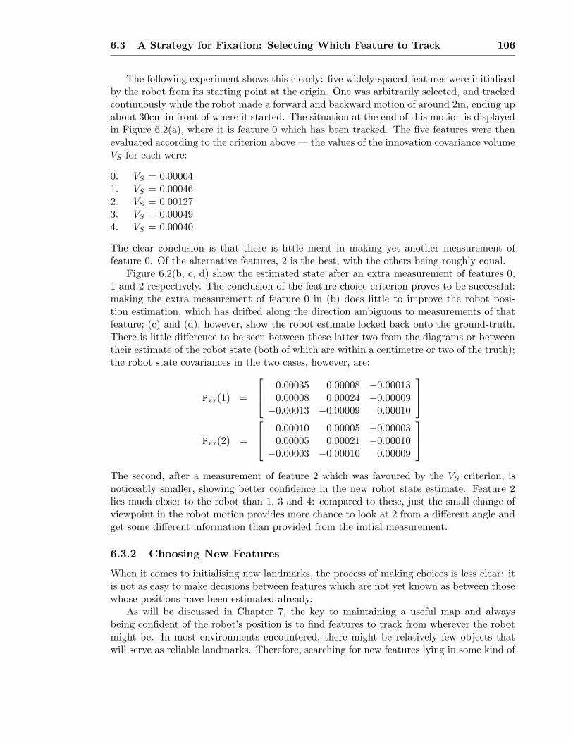
6.3 A Strategy for Fixation: Selecting Which Feature to Track 106
The following experiment shows this clearly: five widely-spaced features were initialisedby the robot from its starting point at the origin. One was arbitrarily selected, and trackedcontinuously while the robot made a forward and backward motion of around 2m, ending upabout 30cm in front of where it started. The situation at the end of this motion is displayedin Figure 6.2(a), where it is feature 0 which has been tracked. The five features were thenevaluated according to the criterion above — the values of the innovation covariance volumeVS for each were:
0. VS = 0.000041. VS = 0.000462. VS = 0.001273. VS = 0.000494. VS = 0.00040
The clear conclusion is that there is little merit in making yet another measurement offeature 0. Of the alternative features, 2 is the best, with the others being roughly equal.
Figure 6.2(b, c, d) show the estimated state after an extra measurement of features 0,1 and 2 respectively. The conclusion of the feature choice criterion proves to be successful:making the extra measurement of feature 0 in (b) does little to improve the robot posi-tion estimation, which has drifted along the direction ambiguous to measurements of thatfeature; (c) and (d), however, show the robot estimate locked back onto the ground-truth.There is little difference to be seen between these latter two from the diagrams or betweentheir estimate of the robot state (both of which are within a centimetre or two of the truth);the robot state covariances in the two cases, however, are:
Pxx(1) =
0.00035 0.00008 −0.000130.00008 0.00024 −0.00009
−0.00013 −0.00009 0.00010
Pxx(2) =
0.00010 0.00005 −0.000030.00005 0.00021 −0.00010
−0.00003 −0.00010 0.00009
The second, after a measurement of feature 2 which was favoured by the VS criterion, isnoticeably smaller, showing better confidence in the new robot state estimate. Feature 2lies much closer to the robot than 1, 3 and 4: compared to these, just the small change ofviewpoint in the robot motion provides more chance to look at 2 from a different angle andget some different information than provided from the initial measurement.
6.3.2 Choosing New Features
When it comes to initialising new landmarks, the process of making choices is less clear: itis not as easy to make decisions between features which are not yet known as between thosewhose positions have been estimated already.
As will be discussed in Chapter 7, the key to maintaining a useful map and alwaysbeing confident of the robot’s position is to find features to track from wherever the robotmight be. In most environments encountered, there might be relatively few objects thatwill serve as reliable landmarks. Therefore, searching for new features lying in some kind of

6.3 A Strategy for Fixation: Selecting Which Feature to Track 107
“optimal” positions relative to the robot might prove futile. The approach we have taken isto consider how to make a choice from an arbitrary set of features which have been newlyinitialised wherever they could be found.
A fact which is initially slightly surprising, but clear when given consideration, is thatthe value of VS for an immediate re-measurement, before the robot has moved, of a featurewhich has just been initialised is always the same, independent of the location of the feature:
VS(new) =4
3π(√
2nσ)3∆α∆e∆γ .
This value is 6.91×10⁻⁵ with the parameters used in our system at the time of experiments(number of standard deviations nσ = 3, estimates of angular measurement errors ∆α =∆e = ∆γ = 0.006). The reason for this is that the uncertainty in the position relativeto the robot of a newly initialised feature is simply the uncertainty in the initialisationmeasurement — and so the innovation covariance when a second measurement is made of itis the sum of this and the uncertainty in the new measurement: the total is simply doublethe single measurement uncertainty. In the normalised (α, e, γ) measurement representationthis amount is constant. So, despite the fact that the uncertainties in (x, y, z) space lookdramatically different for newly initialised features which are close to or far from the robot,in angular space they are all the same. Consider a feature which is very far from therobot, for instance: it will have a large depth uncertainty, represented by an ellipse which iselongated in that direction. The robot can, however, fixate any point along the depth axiswith only small changes in its vergence angle — the same range of changes which span themuch smaller depth uncertainty range of a close feature.
This means that from a selection of newly initialised features, it will not be possible tochoose one to measure first on the same basis as choosing between well-established features:there will not be one feature which as it stands will represent a better measurement than theothers. It is clear, however, that once the robot has made a movement, the fact that it hasthe potential to observe the features from a different viewpoint means that VS will not be thesame in each case. Its value will change depending on how much the view of the feature isdifferent from the original initialising view. We can think of a new measurement uncertaintyellipse in (x, y, z) space intersecting the feature position uncertainty: the measurement willbe particularly valuable if the volume mutually enclosed by both is much smaller than thevolume of the original ellipse. An extreme case would be two elongated ellipses crossing atright angles: the feature position could then be pinpointed very precisely.
So choice between new features depends on some knowledge of the robot’s future motionplan. In our system, the current velocity and steering angle settings and a “number of steps”setting determine the robot’s next motion. Based on these, a prediction can be made ofthe state after the motion by simply applying the prediction stage of the Kalman Filter theappropriate number of times. With this predicted state, VS is evaluated for each of the newfeatures. This reveals which of the features would provide the best one-off measurementafter carrying out the motion blindly: it is the one which the robot will be able to measurefrom the most different viewpoint. This feature can therefore be chosen above the othersfor immediate tracking. Although the repeated measurements provided by tracking arecertainly different from the one measurement at the end of the movement considered in thechoice criterion, for relatively short movements at least we expect that the feature which isbest to track will be the same as that best to measure once.
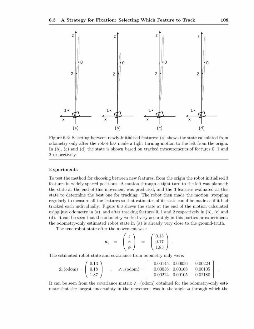
6.3 A Strategy for Fixation: Selecting Which Feature to Track 108
x
1
2
0
z
x
1
2
z
0
x
1
2
z
0
x
z
1
2
0
(a) (b) (c) (d)
Figure 6.3: Selecting between newly-initialised features: (a) shows the state calculated fromodometry only after the robot has made a tight turning motion to the left from the origin.In (b), (c) and (d) the state is shown based on tracked measurements of features 0, 1 and2 respectively.
Experiments
To test the method for choosing between new features, from the origin the robot initialised 3features in widely spaced positions. A motion through a tight turn to the left was planned:the state at the end of this movement was predicted, and the 3 features evaluated at thisstate to determine the best one for tracking. The robot then made the motion, stoppingregularly to measure all the features so that estimates of its state could be made as if it hadtracked each individually. Figure 6.3 shows the state at the end of the motion calculatedusing just odometry in (a), and after tracking features 0, 1 and 2 respectively in (b), (c) and(d). It can be seen that the odometry worked very accurately in this particular experiment:the odometry-only estimated robot state in (a) is already very close to the ground-truth.
The true robot state after the movement was:
xv =
zxφ
=
0.130.171.85
.
The estimated robot state and covariance from odometry only were:
xv(odom) =
0.130.181.87
, Pxx(odom) =
0.00145 0.00056 −0.002240.00056 0.00168 0.00105
−0.00224 0.00105 0.02180
.
It can be seen from the covariance matrix Pxx(odom) obtained for the odometry-only esti-mate that the largest uncertainty in the movement was in the angle φ through which the

6.3 A Strategy for Fixation: Selecting Which Feature to Track 109
robot had turned.The estimated robot state and covariance after tracking features 0, 1 and 2 respectively
were:
xv(0) =
0.130.181.84
, Pxx(0) =
0.00121 0.00073 −0.000140.00073 0.00156 −0.00025
−0.00014 −0.00025 0.00012
xv(1) =
0.130.181.85
, Pxx(1) =
0.00039 0.00011 0.000240.00011 0.00039 −0.000140.00024 −0.00014 0.00035
xv(2) =
0.120.171.85
, Pxx(2) =
0.00105 0.00063 −0.000140.00063 0.00150 −0.00031
−0.00014 −0.00031 0.00014
Now the values obtained in the comparison of features were:
0. VS = 0.001261. VS = 0.003592. VS = 0.00136
A clear favourite emerged: feature 1, with 0 and 2 roughly equal but some way behind.To evaluate whether 1 really was the best feature to track, there is little evidence to bedrawn from the different robot state estimates xv(0), xv(1) and xv(2): all are very closeto the ground-truth in this experiment as was the odometry-only estimate. Looking at thecovariance matrices Pxx(0), Pxx(1) and Pxx(2), it can be seen that measuring any of thefeatures is good for reducing the uncertainty in φ: they all have small (3, 3) elements. Thisis expected: looking at any fixed point while turning will allow a good estimate of the angleto be made. We also see, though, that measuring feature 1 has done a much better job ofreducing the uncertainty in z and x, the estimated 2D coordinates of the vehicle on theground plane — the (1, 1) and (2, 2) elements of Pxx(1) are much smaller than those ofthe other covariance matrices. The fact that feature 1 is much closer to the robot thanthe others has meant that the small movement which the robot has made has produced alarger change in viewpoint of this feature than the others — there has been a chance forthe elevation and vergence angles to change during tracking as well as the large pan axischange experienced when tracking any of the features. The choice criterion for new featurescorrectly identified this feature as best to track for the same reasons.
It may seem from this experiment and that of previous section that it will always bepreferable to use very close features as landmarks: this is not necessarily the case. Forinstance, distant features have the advantage that the same ones can be measured as therobot moves through much larger distances, due to their relatively small change in appear-ance. In the extreme case, GPS has shown that extremely distant beacons in the form ofsatellites can be used for accurate localisation (although with measurements of distance,rather than distance and angle as here). The approach in this thesis treats all features inthe same manner: choices will be made on grounds of how useful they are in informationterms, and it will be seen in the next chapter that distant features often have a part to play.

6.3 A Strategy for Fixation: Selecting Which Feature to Track 110
6.3.3 Continuous Switching of Fixation
In the previous two sections, a “stop and look” approach was assumed: with the robotat a standstill, a known feature can be chosen to give the best update with an immediatemeasurement, or a new feature chosen to give the best update after a predicted motion.There is no significance in the position of the feature: as the robot moves off, the activehead will saccade to fixation and tracking will commence. The robot will then stop after acertain time to plan its next movement and choice of feature.
Now we consider the problem of selecting between features while the robot is actuallymoving. Direct implementation of selection of the feature with the current highest VS is notideal: what happens is that once a measurement has been made of one feature, the criterionsuggests an immediate saccade to another. Once this feature is found, another fixationswitch is required. The result is that the active head is constantly saccading, making aquick measurement and then moving on again.
Our active head is very fast, but it takes a certain amount of time to make a saccade:for two features which are widely separated (one directly ahead of the robot and one at theside for instance), the time from starting to move until a successful measurement is madeof the new feature can be more than half a second. During this time, no measurements arepossible. On the other hand, at the usual tracking rate of 5Hz around 3 measurements couldhave been made if fixation had been maintained on the current feature. These measurementswould each have been less valuable than the one finally obtained of the new feature, but itmight be that together they amount to more.
To incorporate the penalty of saccading into the choice-of-feature criterion, we first re-quire a basis for deciding whether one estimated state is better than another. Rememberingthat total map integrity is what is important, we suggest that in a particular state, whena comparison of the visible features is made, VS(max), the highest VS found, is a goodindicator. If VS(max) is high, there is a measurement which needs to be made urgently tosmooth off the map’s rough edges. If, however, VS(max) is low, the relative positions of all
the features are known well, and the state estimate is good.The essence of our approach to choosing features while the vehicle is moving, therefore,
is to predict the robot and map state at a short time in the future based on either stayingtracking the current feature or a potential saccade to each alternative, and then compareVS(max) for these states to see which is lowest. The “short time in the future” is chosen tobe the length of time in which a saccade and measurement could be successfully completedto any of the features. The steps followed are:
1. Calculate the number of measurements Ni which would be lost during a saccade toeach of the visible features. This is done by estimating the time which each head axiswould need to move to the correct position, taking the largest (usually the pan timesince this axis is the slowest), and dividing by the inter-measurement time interval(0.2s).
2. Identify Nmax, the highest Ni: this is the number of measurements lost in the largestsaccade available.
3. For each feature i, make an estimate of the state after Nmax +1 steps if an immediatesaccade to it is initiated. This consists of making Ni filter prediction steps followed

6.3 A Strategy for Fixation: Selecting Which Feature to Track 111
by Nmax−Ni +1 simulated prediction/measurement updates. A measurement is sim-ulated by updating the state as if the feature had been found in exactly the predictedposition (it is the change in covariance which is important here rather than the actualestimate). An estimated state after the same number of steps is also calculated forcontinued tracking of the currently selected feature.
4. For each of these estimated states, VS(max) is evaluated. The saccade providing thelowest VS(max) is chosen for action; or tracking stays with the current feature if thatVS(max)is lowest.
One important point here is that the efficient updating method of Section 6.2 cannotbe used in this continuous fixation switching framework: we rely on the full state andcovariance being up-to-date at all times.
Experiment with Fixation Switching Between Four Features
Figure 6.4 shows an experiment into continuous fixation switching: four features were ini-tialised, and (a) shows the robot’s trajectory as it started to move forward at about 4cms−1,choosing which features to fixate on as described above. In (b), the values obtained froma straight VS comparison of the four features at each time step are plotted. The four linesshow how uncertainty in the positions of the features relative to the robot vary with time.As would be hoped, there is a general downward trend (from the initial state where all thefeatures have VS = VS(new) as explained in Section 6.3.2), showing that the positions arebecoming more and more certain.
In the early stages of the motion, fixation switches as rapidly as possible between thefour features: only one measurement at a time is made of each feature before attention isshifted to another. In the graph of Figure 6.4(b), a measurement of a particular featureappears as a sharp drop in its VS value. While a feature is being neglected, its VS graduallycreeps up again. This is because the newly-initialised features have large and uncoupleduncertainties: their relative locations are not well known, and measuring one does not domuch to improve the estimate of another’s position. After a while, the feature states becomemore coupled: around step 40, clear zig-zags in the rising curves of neglected features showthat the uncertainties in their positions relative to the vehicle are slightly reduced when ameasurement is made of another feature.
At around step 80, the first clear situation is seen where it becomes preferable to fixateone feature for an extended period: feature 1 is tracked for about 10 steps. This featureis very close to the robot, and the robot is moving towards it: measurements of it providethe best information on the robot’s motion (the motion past feature 0 is rather tangentialand prone to the ambiguity of Figure 5.7). Since the locations of the other features arebecoming better known, their positions relative to the robot are constrained quite well bythese repeated measurements (only a gentle rise in the lines for features 0, 2 and 3 is seenduring this time). Feature 1 actually goes out of the robot’s view at step 101 (the robothaving moved too close to it, violating one of the visibility criteria of Section 4.1.2), andbehaviour returns to quite rapid switching between the other features.
The robot was stopped at the end of this run with state estimates intact. It was thendriven back to near the origin in a step-by-step fashion, making further dense measurementsof all of the features along the way. The result was that once it was back at its starting

6.3 A Strategy for Fixation: Selecting Which Feature to Track 112
x
0
1
2
3
z
0 30 60 90 120
Step Number
2e-05
3e-05
4e-05
5e-05
6e-05
7e-05
8e-05
9e-05
Inno
vatio
n C
ovar
ianc
e V
olum
e
Feature 0Feature 1Feature 2Feature 3
(a) (b)
z
x
0
1
2
3
0 60 120 180 240 300
Step Number
2.7e-05
3.5e-05
4.3e-05
5.1e-05
5.9e-05
6.7e-05
Inno
vatio
n C
ovar
ianc
e V
olum
e
Feature 0Feature 1Feature 2Feature 3
(c) (d)
Figure 6.4: Experiments in continuous fixation switching: for the trajectory in (a), asthe robot moves in the region of 4 newly-initialised features, (b) compares the innovationcovariance volume VS for the features as fixation switches between them. In a secondmotion in (c), the world positions of the features are more accurately known, and (d) againcompares VS .
6.4 Conclusion 113
point, feature estimates had been very well established. It was from this point that a secondcontinuous switching run was initiated: the trajectory and the now accurately estimatedfeature positions are shown in Figure 6.4(c), and a graph of the feature comparison in (d).
This second graph is dramatically different from the first: in the early stages, low VS
values for all the features are now maintained by extended periods of tracking one feature(feature 1 again). The strong coupling now established between feature estimates meansthat if the robot position relative to one can be well estimated, as is the case when thenicely placed feature 1 is tracked, its position relative to the others will be as well. There isthe occasional jump to another feature, appearing as spikes in the traces at around steps 70and 90. Just after step 120, feature 1 goes out of view, and a period of rapid switchingoccurs. None of the remaining features on its own provides especially good overall robotposition information, and it is necessary to measure them in turn.
Feature 0 goes out of view (due to too large a change in viewing angle) at step 147.After this, only the distant features 2 and 3 remain for measurements. It is noticeable thatthroughout the graph these two have been locked together in their VS values: measurementsof them provide very similar information due to their proximity, and there is little need toswitch attention between them. These features finally go out of view at about step 270,leaving the robot to navigate with odometry only.
Experiment with Varying Head Performance
Our active head is very fast, but it was interesting to see how the continuous fixationswitching criterion would direct the actions of a head with lower performance. To simulatethis, the control parameters of Yorick 8-11 were tuned down to reduce its performance byabout 30%. This change was reflected in the fixation switching method, where estimates ofthe time taken to make saccades were increased by appropriate amounts.
An experiment was performed with the head in both its normal configuration and in thetuned-down version. Two distant features (the same ones which were features 2 and 3 in theprevious experiment) were initialised from the origin and the robot drove straight forward,switching attention between them. Graphs from the two runs can be seen in Figure 6.5,where (a) is at full-performance and (b) tuned-down. The differences are slight but clear:the traces for the two features are bound more tightly together in (a) in the early stageswhere repeated switching occurs: the more rapid saccades available allow the robot to keepits uncertainty in the two features close. Later on, when the feature estimates have beencoupled, we see fewer fixation switches in (b), where the larger penalty of saccades meansthat it is worthwhile tracking one feature for longer. Note that the particularly large spikein graph (a) at around step 150 is caused by some failed measurements.
6.4 Conclusion
We have shown that features can be tracked continuously in an efficient manner as therobot moves, and that intelligent choices can be made about which features should betracked when to provide good navigation information. In the next chapter, these methodswill be integrated into a system for automatic map-maintenance and localisation for use ingoal-directed navigation.
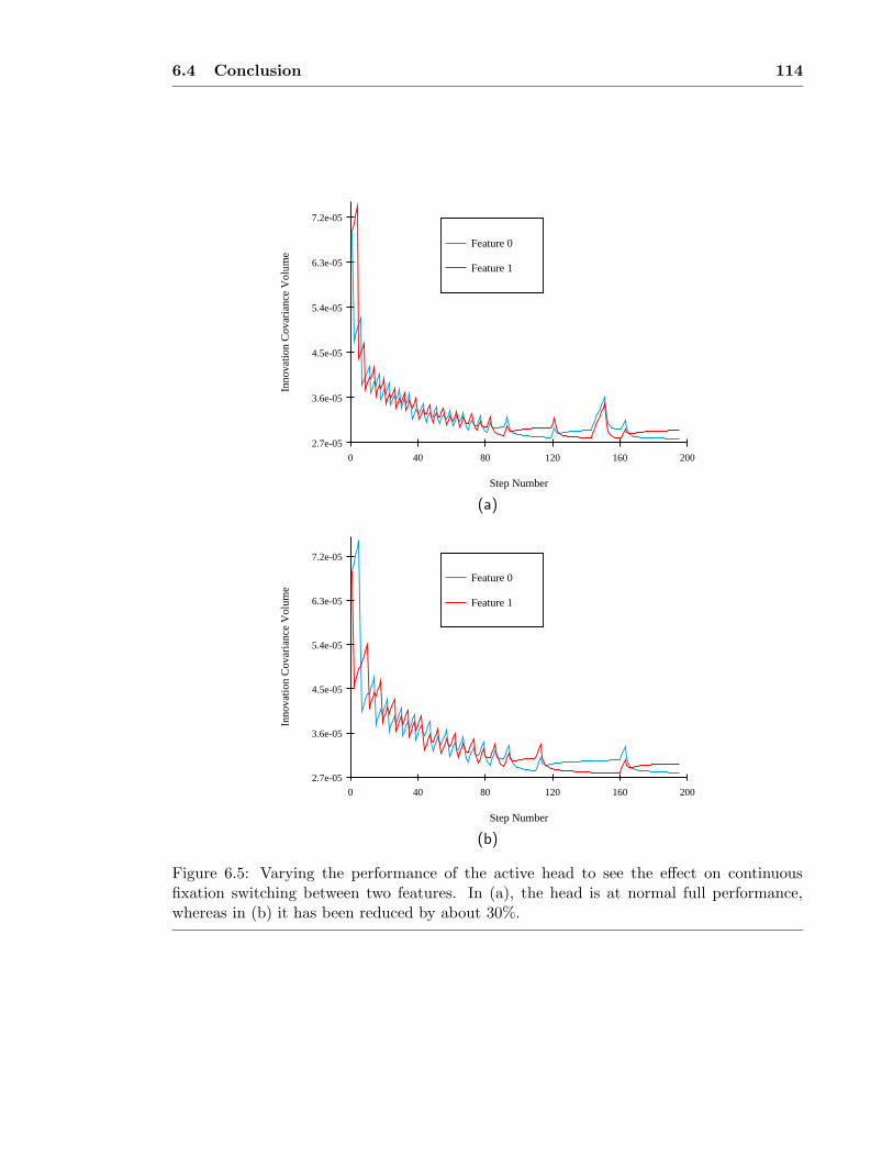
6.4 Conclusion 114
0 40 80 120 160 200
Step Number
2.7e-05
3.6e-05
4.5e-05
5.4e-05
6.3e-05
7.2e-05
Inno
vatio
n C
ovar
ianc
e V
olum
e
Feature 0
Feature 1
(a)
0 40 80 120 160 200
Step Number
2.7e-05
3.6e-05
4.5e-05
5.4e-05
6.3e-05
7.2e-05
Inno
vatio
n C
ovar
ianc
e V
olum
e
Feature 0
Feature 1
(b)
Figure 6.5: Varying the performance of the active head to see the effect on continuousfixation switching between two features. In (a), the head is at normal full performance,whereas in (b) it has been reduced by about 30%.

6.4 Conclusion 115
One question arises concerning the choice-of-feature criteria derived in Section 6.3: theassumption has been made that the best measurement to make is that which can in onestep reduce map uncertainty the most — and this will be a measurement whose result isuncertain. In Section 6.3.3, the factor of potential measurements being weighted against bythe time necessary to saccade to a new feature was taken into account, but what has notbeen considered is the fact that the most uncertain measurements will take the most com-putational time to acquire, in terms of large image regions which will have to be searched.In a system such as ours with mechatronic active vision, this factor is perhaps insignifi-cant compared with the effort of changing fixation to another feature. However, with moregeneral active sensors, such as a digitally movable window within an image from a staticcamera, is there an optimum size of search window to investigate, or is it just as useful tomake many fast, predictable measurements rather than a few unpredictable ones?

7Autonomous Navigation
In this final major chapter, we will look at how the methods developed in this thesis willform the key parts of a useful autonomous robot navigation system using active vision. Asdiscussed in Chapter 1, it must be remembered that navigation in unknown surroundingsis a challenging goal, and one which has not yet been achieved satisfactorily by mobilerobots operating without external assistance. Robots have been built which can move au-tonomously for long periods in unfamiliar areas, such as the lawn-mowing robot mentionedin Chapter 1, but not while monitoring their location relative to any fixed axes, which weargue is necessary for many tasks. Those robots which have shown success in navigatingwith respect to fixed axes have usually made use of prior knowledge about the environment,such as beacons in known positions.
If we assume that the robot’s overall goal is decided by some other process — perhapsa pre-programmed position command from a human operator, a target-seeking behaviourpulling the robot towards some stationary or moving object, a desire to move in a loopedpatrolling motion, or an exploration behaviour pulling it towards new areas — what capa-bilities does it need to accomplish that goal? It must be able to:
• Monitor its position as it moves.
• Plan and control its movement.
• Avoid obstacles.
The first of these is what the main part of this thesis is about: by building and using a mapof landmark features, the robot is able to obtain much better localisation information thanit would otherwise obtain from solely odometry. We will look in Section 7.1 at how a usefulmap is automatically generated and maintained in our system.

7.1 Maintaining a Map 117
The second capability, planning and controlling motion, is perhaps relatively simple inrelation to the other two, particularly in the case of our robot which is assumed to moveon a perfect planar surface. In Section 7.2, a simple method is described via which therobot may either steer towards a waypoint specified by ground-plane coordinates, or steersafely around a known obstacle. It is shown how these types of motion can be combinedsequentially to produce compound movements.
In Section 7.3 we present an experiment which demonstrates automatic map-main-tenance and motion control as the robot moves autonomously up and down a corridor-likearea, navigating to specified waypoints and matching features after periods of neglect torecognise previously visited areas. A comparison is made with a repeat of the experimentwhere the robot did not use visual map-building and relied unsuccessfully on its odometry.
Section 7.4 concludes the chapter with discussion and several experiments indicatingwhat additional capabilities it is felt are needed to take autonomous robots into the realworld, with vision as the primary sensing modality. Position-based navigation is contrastedwith a context-based methodology, and the route to their fusion in truly capable robots isdiscussed.
7.1 Maintaining a Map
We have seen from the experiments of the previous two chapters that robot localisationestimation is always improved by tracking fixed landmarks in the world. Further, the bestscenario is to make repeated measurements of the same set of landmarks as the robot moveswithin a particular area, and come back to previously seen landmarks when an area is re-visited. This is possible if a map of features is generated and maintained in which eachcan be relied upon to be matchable and have a well-known location. The Kalman Filter ofChapter 5 ensures that the best use will be made of whatever measurements are obtainedto build a consistent map, and it was shown how features can be added or deleted at will;in this section we will consider how choices should be made about which features to includein the map.
As mentioned in Section 6.3.2, the likelihood is that there will only be a limited numberof features in a particular environment which will make good landmarks, in terms of havingsufficient contrast with the background and viewpoint-invariant appearance to be matchedreliably. For this reason, initialisation of new features is performed somewhat arbitrarily:no attempt is made to search for features in particular positions. The active head is directedto view the scene to the left, right and straight ahead of the robot, and at each of thesepositions the patch-finding operator of Section 4.1.1 is applied in the images obtained andan attempt is made to initialise a feature if a good patch is found. In this way, up to 3widely-spaced new features will be added to the map. A choice of which of these to trackfirst is then made as in Section 6.3.2.
During general autonomous navigation, choice of the feature to track at a given timeis made according to the VS criterion presented in Section 6.3.1: each feature in the mapis tested for its expected “visibility”, meaning whether the robot is estimated to be withinan area from which it will have a view of the feature which is sufficiently close in distanceand angle to the viewpoint from which the feature was initialised (see Section 4.1.2). Thevisible feature which will provide the most information is then selected for measurement.

7.1 Maintaining a Map 118
When is it time to initialise more new features? Obviously at the start of a journey,when no landmarks are known. After this, the map-building formulation allows more to beadded at any time. In some ways, it is preferable for the map not to be too dense: having alarge number of landmarks means that fewer measurements can be made of each one, andtheir positions will be less well known. The automatic feature selection criterion will choosethe newer, less well-known features, and while these are being tracked the well-known onescan go out of view, meaning that the robot position estimate will tend to drift. Also, it ispreferable in terms of efficiency to keep the complexity of the map down.
Remembering the importance of repeated switching of tracking demonstrated in theexperiments of the previous chapter, but also aiming to keep the map relatively sparse, itwas decided that at least two features should be available for measurements at a given time.Therefore, the robot stops and initialises new features if, due to motion into a new area orthe deletion of features, a point is reached where less than two are visible.
It was mentioned in Chapter 4 that when a feature is initialised no attempt is made todetermine whether it will make a durable landmark. This is not strictly the case, becausethe repeated stereo matching between the robot’s two cameras necessary to fixate a featureduring initialisation ensures that it at least has viewpoint-invariance across the relativelysmall inter-ocular baseline. However, newly-initialised features will in general not have beenconfirmed as good landmarks. The natural approach which can be taken to decide whetherthey are is to see how successfully they can be tracked. Making repeated measurementsof a feature under the constraints of the Kalman Filter means that by definition it makesa good landmark: it must be a fixed point in 3D space which does not change greatly inappearance with viewpoint. It is possible to conceive of features which could deceive thefilter by remaining trackable while changing their position: an apparent corner feature atan occlusion boundary, for instance, might move in 3D by a small enough amount withviewpoint changes to convince the robot that the feature was actually stationary and therobot’s motion was slightly different than would otherwise be calculated. Fortunately, theseare rare in practice, and anyway with frequent enough measurements of a range of otherfeatures the robot’s motion can be checked against other references.
To decide which features to keep in the map, therefore, for each one counts are main-tained of the number of attempted measurements and the number of successful measure-ments. Since measurements are only attempted from robot positions form which the featureis expected to be “visible”, the ratio of these gives a score reflecting how reliable the fea-ture is. A feature is deleted from the map if, after at least 10 attempted measurements,the successful measurement ratio ever falls below 0.5. Deletion will occur if the feature isfrequently occluded as well is if it is a “bad” feature as discussed above.
The criterion for deleting features from the map works well in practice. If a feature hasbeen successfully measured a lot of times from within its area of expected visibility, it buildsup a high scores for both attempted measurements and successful measurements: the ratioof these is then quite stable. A few missed measurements of the feature do not lead to itsdeletion, and rightly so: the reason for these missed measurements is something other thanthe feature’s quality. It is possible that the robot has temporarily badly estimated its ownlocation and assigned too much certainty to this estimate. The failed measurements confirmthis, and the robot’s position uncertainty will grow (in the standard prediction stage of thefilter), hopefully to the point where the feature, still safely in the map, will lie within thelarger search regions generated.

7.2 Controlling the Robot’s Motion 119
In summary, the approach taken to automatic map maintenance is:
• From the visible features, choose the current one to track according to the informationcriteria of Section 6.3.
• If fewer than two features are currently visible, initialise some new ones.
• If more than half of the attempted measurements of a feature have failed (after atleast 10 attempts), delete it.
The results in practice will be seen in Section 7.3.
7.2 Controlling the Robot’s Motion
With the information from its localisation and map-building system, the robot is in aposition to control its movements either in relation to the world coordinate frame or inrelation to features in the map. A similar approach is taken in both cases, which makesuse of the ideas of visual servoing [44]: if an object to be interacted with is tracked, thesmall changes in the measurement of its position at each step can be directly coupled tothe control system of the robot attempting the interaction. The absolute locations of eithermanipulator or objects need not be known.
If a feature can be tracked at fixation by an active camera or a stereo head, servoinginformation is directly available in a very useful angular form. The values from the jointangles provide proprioceptive information which abstracts and replaces the original imagemeasurements. The next section shows how the robot can steer around an obstacle featurewhich is tracked at fixation using our normal filter approach (Section 7.4 will consider howto incorporate this behaviour into autonomous navigation), and how a similar approach canalso be used to steer the robot towards specified waypoints on a desired trajectory.
7.2.1 Steering Control
A simple law is used to control the robot’s steering angle when navigating either around anobstacle [6] or towards a journey waypoint.
Steering Around An Obstacle
Referring to Figure 7.1, an obstacle exists at O which the robot must avoid by a safe radiusR. From a fixated stereo measurement, the pan angle α and distance D to the feature arerecovered. It can be seen that if the robot were to turn on the spot about the head centrethrough the angle α− sin−1 R
D, it would be directly lined up to drive along a tangent to the
safe-radius circle. Rather than do this, the angle s of the steering wheel at the back of thevehicle is set to be proportional to this required correction in heading:
s = κ(α − sin−1 R
D) . (7.1)
κ is a constant of proportionality called the steering gain. As the robot starts to drivetowards the obstacle steering according to this law, repeated measurements are obtainedfrom the active head, and the steering angle continuously changes. The result is a smooth

7.2 Controlling the Robot’s Motion 120
R
D
O
v
s
sin (R/D)−1
h
α
Figure 7.1: Steering at a safe radius R around an obstacle at O: alpha is the pan or gazeangle to fixate on the feature, and D is its distance from the head centre. s is the steeringangle derived.
steering trajectory directing the robot around the obstacle. The value of κ affects howurgently the robot will turn towards the tangent circle — low values produce more gentletrajectories. Figure 7.2 shows the action of this steering law in real experiments wherethe robot steered around an obstacle with different initial relative obstacle/robot positionsand different values of gain κ. The obstacle was a clearly visible feature on the cornerof a laboratory bench (the top four images of Figure 6.1 were taken from one of theseexperiments), chosen because it was matchable over the long robot motions involved.
Steering Towards a Waypoint
With a small adaption, the steering law can be used to direct the vehicle smoothly towardsa specified waypoint rather than around an obstacle, in a form of control relying on therobot’s world position estimation. The ground-plane coordinates (Zw, Xw) of the pointthrough which it is desired that the robot should pass are used to calculate the pan angleαw to which the active head would have to be turned to observe a feature at that positionaccording to the current robot location estimate. The steering angle is then set proportionalto this, but without the safe radius offset of Equation 7.1:
s = κwαw . (7.2)
This law will tend to steer the robot directly towards the waypoint, the value of κw againplaying the role of a gain parameter affecting the urgency of steering.
A long planned trajectory consists of a series of waypoints to be reached in sequence.A waypoint is said to have been reached if the robot’s estimated location lies within asmall radius of the waypoint position, and attention is now turned to the next one. If thepan angle to a waypoint is ever so large as to make the steering angle s calculated from

7.2 Controlling the Robot’s Motion 121
x
z
x
z
x
z
x
z
x
z
x
z
x
z
x
z
x
z
κ = 0.5 κ = 1.0 κ = 1.5
Figure 7.2: Robot trajectories produced by the the steering law with different values of gainκ and different obstacle positions.
Equation 7.2 greater than π/2, s is limited to this value: the robot makes a turn on thespot. This is most likely to occur when a new waypoint has just become the steering goal.
A note on velocity control: during map-building, the robot travels at a velocity fixedat the start of the run, but it moves more slowly when sharp turns are called for. Thismakes tracking features slightly easier for the filter since their angular movement betweenmeasurement steps, and therefore the area of image search regions, are reduced. Of course,the choice of velocity does not affect the trajectory of the robot.
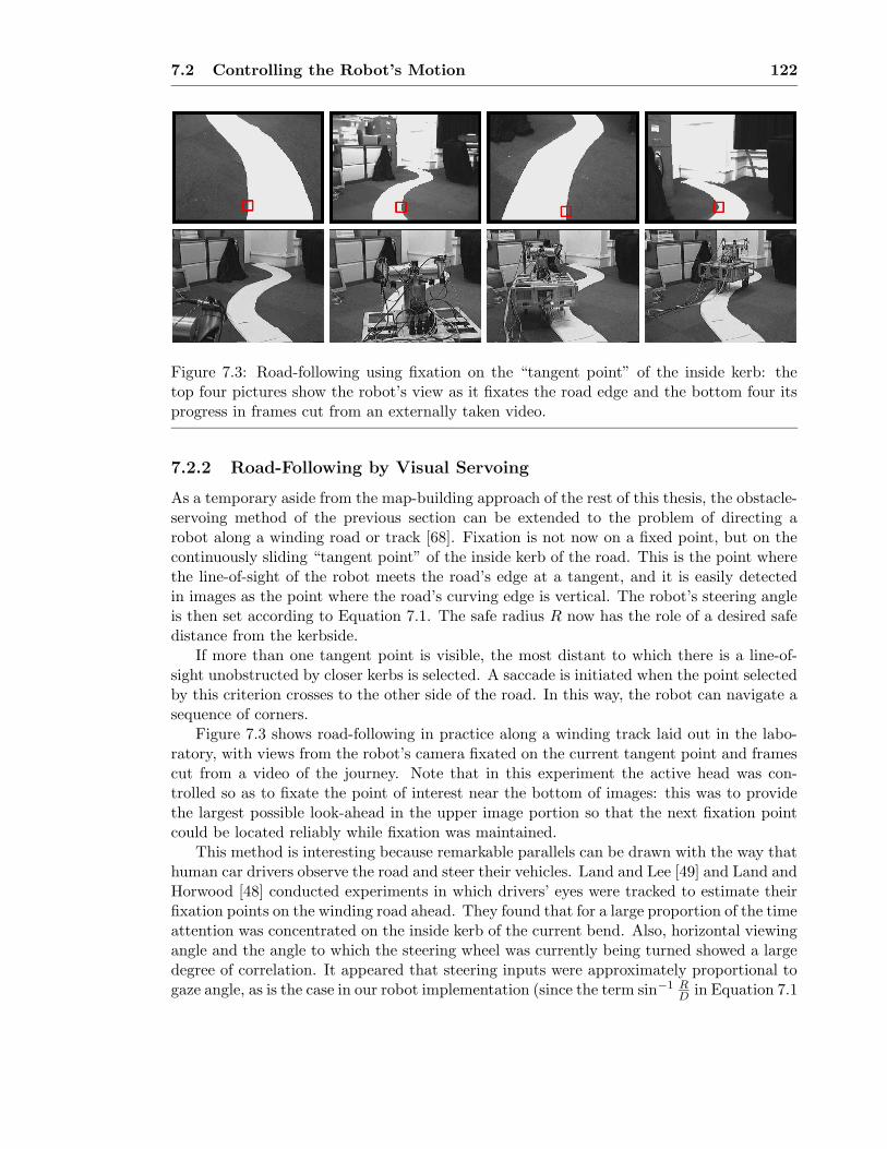
7.2 Controlling the Robot’s Motion 122
Figure 7.3: Road-following using fixation on the “tangent point” of the inside kerb: thetop four pictures show the robot’s view as it fixates the road edge and the bottom four itsprogress in frames cut from an externally taken video.
7.2.2 Road-Following by Visual Servoing
As a temporary aside from the map-building approach of the rest of this thesis, the obstacle-servoing method of the previous section can be extended to the problem of directing arobot along a winding road or track [68]. Fixation is not now on a fixed point, but on thecontinuously sliding “tangent point” of the inside kerb of the road. This is the point wherethe line-of-sight of the robot meets the road’s edge at a tangent, and it is easily detectedin images as the point where the road’s curving edge is vertical. The robot’s steering angleis then set according to Equation 7.1. The safe radius R now has the role of a desired safedistance from the kerbside.
If more than one tangent point is visible, the most distant to which there is a line-of-sight unobstructed by closer kerbs is selected. A saccade is initiated when the point selectedby this criterion crosses to the other side of the road. In this way, the robot can navigate asequence of corners.
Figure 7.3 shows road-following in practice along a winding track laid out in the labo-ratory, with views from the robot’s camera fixated on the current tangent point and framescut from a video of the journey. Note that in this experiment the active head was con-trolled so as to fixate the point of interest near the bottom of images: this was to providethe largest possible look-ahead in the upper image portion so that the next fixation pointcould be located reliably while fixation was maintained.
This method is interesting because remarkable parallels can be drawn with the way thathuman car drivers observe the road and steer their vehicles. Land and Lee [49] and Land andHorwood [48] conducted experiments in which drivers’ eyes were tracked to estimate theirfixation points on the winding road ahead. They found that for a large proportion of the timeattention was concentrated on the inside kerb of the current bend. Also, horizontal viewingangle and the angle to which the steering wheel was currently being turned showed a largedegree of correlation. It appeared that steering inputs were approximately proportional togaze angle, as is the case in our robot implementation (since the term sin−1 R
Din Equation 7.1

7.3 Automatic Position-Based Navigation 123
becomes negligibly small when the distance D to the fixation point is large compared withthe safe distance R, which is true in real driving).
7.3 Automatic Position-Based Navigation
Returning to our main theme, using automatic feature-selection, map maintenance andsteering capabilities, the robot is in a position to perform autonomous position-based nav-igation. A trajectory is specified as a sequence of waypoints in the world coordinate framethrough which the robot is desired to pass. The robot moves in steps of approximately twoseconds duration. Before each step, feature selection chooses the best landmark to trackduring the movement, and features are added to or deleted from the map if necessary. Asthe robot drives, making measurements of the chosen feature and updating the localisationfilter at 5Hz, the steering angle is continuously set to the appropriate value to reach thenext waypoint.
In an experiment, the instructions given to the robot were to head in sequence from itsstarting point at (z, x) = (0, 0) to the waypoints (6, 0.4), (6, 0), and finally (0, 0) again (inmetre units). This experiment was designed to prove again the system’s ability to returnto a previously visited area and recognise it as such, but now using a map which wasgenerated and maintained completely automatically. Note that the extra waypoint (6, 0.4)was specified simply to ensure that the robot turned in a way which was predictable anddid not tangle its umbilical cable.
7.3.1 Using Odometry Only
To first demonstrate the real need for vision or some other kind of sensing in a robotmotion of this kind, the experiment was run with no map-building and the robot relying onodometry only for its position estimation. This run was the same in other respects to thefull experiment below (the robot moved in the same kind of steps and controlled its motionin the same way).
The state at several numbered steps is shown in Figure 7.4. There is quite a largeamount of drift between the ground-truth and estimated robot positions from early on inthe motion, and with no feature measurements this is never rectified. By step (64), theexperiment had to be stopped because although the estimated state was that the robot washeading right down the centre of the corridor, it was actually veering off to the side andwas about to crash. The (z, x, φ) true and estimated robot positions, and the covariance ofthe estimate, were:
xv =
2.89−0.29−2.85
, xv =
2.720.05
−3.12
, Pxx =
0.0018 −0.0010 0.0005−0.0010 0.0151 −0.0039
0.0005 −0.0039 0.0038
.
The estimation is particularly bad with respect to the robot’s orientation φ, where a dis-crepancy of 0.27rad or around 15◦ is seen. Of course, the system knows that its positionestimate is unreliable, and the estimated position covariance is large (although not quite aslarge as it should be in this case to account for the discrepancy, showing potential under-setting of noise in the vehicle motion model, or more likely that the motion noise model is
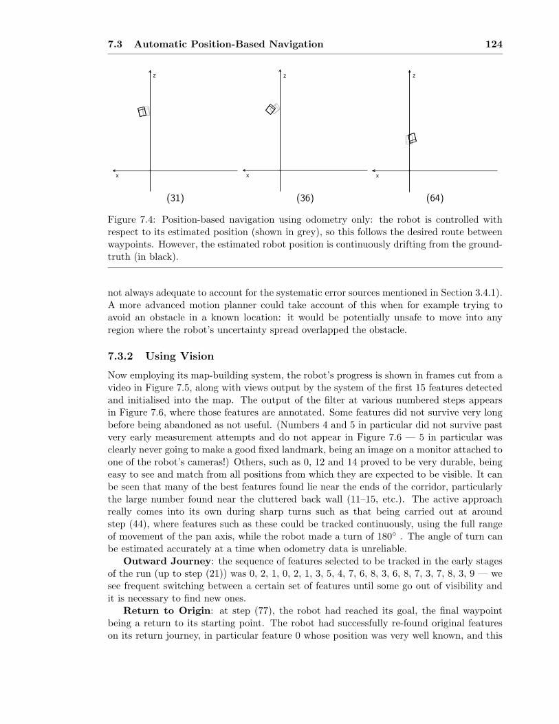
7.3 Automatic Position-Based Navigation 124
x
z
x
z
x
z
(31) (36) (64)
Figure 7.4: Position-based navigation using odometry only: the robot is controlled withrespect to its estimated position (shown in grey), so this follows the desired route betweenwaypoints. However, the estimated robot position is continuously drifting from the ground-truth (in black).
not always adequate to account for the systematic error sources mentioned in Section 3.4.1).A more advanced motion planner could take account of this when for example trying toavoid an obstacle in a known location: it would be potentially unsafe to move into anyregion where the robot’s uncertainty spread overlapped the obstacle.
7.3.2 Using Vision
Now employing its map-building system, the robot’s progress is shown in frames cut from avideo in Figure 7.5, along with views output by the system of the first 15 features detectedand initialised into the map. The output of the filter at various numbered steps appearsin Figure 7.6, where those features are annotated. Some features did not survive very longbefore being abandoned as not useful. (Numbers 4 and 5 in particular did not survive pastvery early measurement attempts and do not appear in Figure 7.6 — 5 in particular wasclearly never going to make a good fixed landmark, being an image on a monitor attached toone of the robot’s cameras!) Others, such as 0, 12 and 14 proved to be very durable, beingeasy to see and match from all positions from which they are expected to be visible. It canbe seen that many of the best features found lie near the ends of the corridor, particularlythe large number found near the cluttered back wall (11–15, etc.). The active approachreally comes into its own during sharp turns such as that being carried out at aroundstep (44), where features such as these could be tracked continuously, using the full rangeof movement of the pan axis, while the robot made a turn of 180◦ . The angle of turn canbe estimated accurately at a time when odometry data is unreliable.
Outward Journey: the sequence of features selected to be tracked in the early stagesof the run (up to step (21)) was 0, 2, 1, 0, 2, 1, 3, 5, 4, 7, 6, 8, 3, 6, 8, 7, 3, 7, 8, 3, 9 — wesee frequent switching between a certain set of features until some go out of visibility andit is necessary to find new ones.
Return to Origin: at step (77), the robot had reached its goal, the final waypointbeing a return to its starting point. The robot had successfully re-found original featureson its return journey, in particular feature 0 whose position was very well known, and this

7.3 Automatic Position-Based Navigation 125
0 1 2 3 4
5 6 7 8 9
10 11 12 13 14
Figure 7.5: Frames from a video of the robot navigating autonomously up and down thecorridor where the active head can be seen fixating on various features, and fixated viewsfrom one of its cameras of the first 15 features initialised as landmarks. The time taken forthe return journey was about 8 minutes.
meant its position estimate was good. What is very appealing is that the choice of featurecriterion described in Section 6.3 had demanded re-measurement of these early featuresas soon as they became visible again, due to the drift which had occurred between therobot position estimate and the world coordinate frame. Generally, the uncertainty in therelative positions of features and the robot, and therefore the VS score indicating the valueof measuring them, will increase with the amount of distance travelled since they were lastmeasured. This gives the system a natural tendency to re-register itself with features seenearlier whenever possible and create a tightly known and globally consistent map.
The robot’s true position relative to the gridded floor was measured here, and can be

7.3 Automatic Position-Based Navigation 126
x
z
1
02
7
z
x
8
6
3
x
z
10
9
(1) (10) (21)
x
z
1113
12
1415
x
z
x
z
(31) (44) (77)
x
z
x
z
(124) (179)
Figure 7.6: Numbered steps in autonomous navigation up and down a corridor. Grey showsthe estimated locations of the vehicle and features, and black (where measured) the truevehicle position. The furthest features lie at z ≈ 8m.
compared with the estimated state and its covariance:
xv =
0.06−0.12
3.05
, xv =
0.15−0.03
2.99
, Pxx =
0.0003 0.0001 −0.00010.0001 0.0001 −0.0001
−0.0001 −0.0001 0.0002
The estimate is much better than at the same point in the odometry-only experiment,although the covariance matrix is again a little too small, showing slight over-confidence in
7.4 Fully Autonomous Navigation 127
the estimate.Repeat Journey: to underline the usefulness of the map generated, the experiment
was continued by commanding the robot back out to (z, x) = (6, 0), then home again to(0, 0). In these further runs, the system needed to do far less map-building since a largenumber of features was already known about along the trajectory. It can be seen that manyof the features previously found survive right until the end of this final run, although thefallibility of some is found out with the further measurements and they are deleted. At(6, 0), step (124), the robot’s true position was z = 5.68m, x = 0.12m, φ = 0.02rad, andestimated state was z = 5.83m, x = 0.00m, φ = -0.02rad. At (0, 0) again, step (179), thetrue position of z = 0.17m, x = -0.07m, φ = -3.03rad compared with the estimate z = 0.18m,x = 0.00m, φ = -3.06rad. This is very impressive localisation performance considering thatthe robot had travelled a total distance of around 24m by this stage.
7.4 Fully Autonomous Navigation
Simply controlling the robot with respect to position waypoints specified in the world co-ordinate frame, as in the previous experiment, is useful but quite limited, even when therobot is required just to move along a pre-ordained path. The problems are:
• Once the robot is some distance from its starting point, its position estimate relativeto the world frame will be unreliable, and so manoeuvring such that the estimatedposition passes through world waypoints will not be accurate.
• While it is using visual landmarks for localisation, the robot is effectively still movingblindly in position-based navigation. No attempt is made to check that the areas tobe passed through are safe and free of obstacles, or that particular regions of interesthave been reached.
Consider an example application: a robot is required to make autonomous inspection toursof a factory along a pre-ordained route. This could be implemented by specifying waypointsrelative to a ground-plan of the factory, and commanding the robot to visit them in sequence,performing map-building as usual. The waypoints might lie at the centres of intersectionsin the factory’s corridor system.
The robot would set off and happily negotiate the corridors near to its origin whereit is able to measure its position accurately — just as in Section 7.3. We note from theexperiment in that section, however, that when the robot had reached its furthest pointfrom the origin, a distance of only about 6m, its z and x position estimates were botharound 15cm from the ground-truth. This is not due to an inadequacy of the filter, which isdoing the best job possible with the information is has, but rather a consequence of the factthat while only using automatically-acquired landmarks many measurements have to becompounded to produce a position estimate out here, as discussed in Section 5.2.1. Whenthe robot travelled farther than this, its estimate would become dangerously uncertain (ifits transverse position estimate was incorrect by around a metre, for example, the robotwould be in danger of crashing into the sides of most corridors).
In Section 7.4.1, we will describe one way in which position-based control can be im-proved in certain environments by providing a small amount of prior information in the formof a few known features, allowing the robot to estimate its position relative to the world
7.4 Fully Autonomous Navigation 128
frame much better over a wide area. However, this is certainly not the generally-applicablesolution which will allow autonomous navigation in many situations. Even when the envi-ronment is well-known beforehand, this method does not allow for changes to be dealt with,such as the introduction of an obstacle. Further, it requires a very accurate description ofthe relative locations of the known features introduced, which will not be available in mostsituations. If the world positions of the known features are inaccurate, the robot will notbe able to find them, or worse be misled by measurement of them.
A more sensible approach is to work towards supporting the same kind of context-basedrather than position-based navigation which humans use in known areas. As discussedin Chapter 5, it does not seem that humans have, or necessarily need, much idea of theglobal relationships between navigational landmarks, and the example of moving arounda well known city was given — streets are located and followed one-by-one, with only therelationships between neighbours needing to be well known. Some success has already beenreported in this type of robot navigation. At the company Applied AI Systems in Canada,a Non-Cartesian Robotics approach based on the subsumption architecture of Brooks [14]has used topological maps and neural-network based visual landmark recognition to guideautonomous robots around simple paths. Their robots do not have an estimation of theiroverall location in a world frame, but know how to move from one landmark to the next. Wewill look in Section 7.4.3 at whether it is possible or sensible to integrate this methodologywith our map-building and localisation system.
The problem of classifying free space/obstacle regions and the ways in which this couldbecome part of an overall navigation system using active vision is investigated in Sec-tion 7.4.2.
7.4.1 Incorporating Known Features into Map-Building
Position-based navigation is directly aided by providing the robot with extra information onits world-frame location, especially when far from its starting point. This can be achievedby providing it with the whereabouts of some known features in the environment as it setsout.
To initialise a known feature, an image patch representing it must be obtained (in ourexperiment by wheeling the robot to near the objects chosen and “taking a picture” with itscameras), and its world position measured. In an environment with a known ground-plansuch as a factory, this could easily be obtained. A slight problem arises here because weare enforcing an abstracted view of the true position of a feature on the system, as wasmentioned in Section 5.4.1: it is difficult to specify the exact location of a landmark in thesame way as the robot would see it. With careful choice of feature, however, we can hopeto get very close.
The measured feature location is initialised directly into the estimated state vector asthe coordinates yi of a feature i. To tell the system that the location of this feature isperfectly known, its covariance Pyiyi
is set with all elements equal to zero, along with thecross-covariances between the feature state and that of the vehicle and other features. Inprediction and measurement updates, the filter copes with these perfectly known landmarkswith no difficultly: once initialised, they can be treated in exactly the same way as auto-matically acquired, uncertain features. In normal filter updates, as should correctly occura perfect feature never becomes tangled with the other estimates, in that the covariance

7.4 Fully Autonomous Navigation 129
0
1
x
z
2
x
z
1
0
2
x
z
2
0
1
x
z
1
0
2
(7) (37) (55) (98)
Figure 7.7: Automatic position-based navigation with 3 known features (0, 1 and 2). Highlocalisation accuracy can now be achieved over a wider range of robot movement.
elements relating to it remain at zero throughout.There have of course been many approaches to robot localisation using known beacons.
Sometimes these are artificially placed into an environment, such as GPS satellites or bar-codes readable by a laser scanner, and sometimes they are naturally occurring featureswhich are known to the robot in the form of a prior map. When all landmarks usedfor navigation are in known positions, the localisation problem becomes relatively simple,and one which has been well tackled [27]. In the approach in this section, we do notpropose to form a full map of known landmarks, but just show that a small number canbe seamlessly incorporated into an automatically-generated map of uncertain features toimprove localisation performance in an easy step.
Experiment with Known Landmarks
An autonomous experiment was conducted where the robot made a similar movement tothat in the experiment of Section 7.3, but now with 3 known features in the map as it setout. These lay to one side of the corridor, and are labelled as 0, 1 and 2 in the pictures ofFigure 7.7 showing the progress of the experiment.
In just the same way that in the experiment of Section 7.3 the automatic feature-choicecriterion selected features not measured for a long time whenever possible, in this experimentthe known features were selected as soon as they became visible, showing the drift whichwas occurring in the robot’s estimation relative to the world frame. The benefit of theknown features was to improve world-frame localisation accuracy when the robot was a

7.4 Fully Autonomous Navigation 130
y
z
32Window
Approximate Position of Light
Figure 7.8: A virtual feature: 32 is a reflection in a window of an overhead light. Its positionin the map lies outside of the laboratory, but it still acts as a stable landmark.
long way from its origin. At step (37), when the robot was at it farthest distance from theorigin, its ground-truth location was measured. The true and estimated locations and theestimate covariance were:
xv =
5.830.01
−0.01
, xv =
5.810.01
−0.02
, Pxx =
0.00022 0.00004 0.000000.00004 0.00010 0.000050.00000 0.00005 0.00007
.
This accuracy, to within a couple of centimetres, vastly improves on that achieved at asimilar position in the experiment of Section 7.3 with no known features (step (124) inFigure 7.6). It can also be seen that automatic features initialised when the robot is in thisposition are much more certain now: the features at the far end of the corridor (high z)in Figure 7.7 have much smaller ellipses than those in Figure 7.6. Features near to knownfeatures become very well-known themselves.
Something interesting arising in this experiment (coincidental to the use of known fea-tures) was the use of a virtual feature as a landmark. The experiment was carried out atnight under artificial lighting, and feature 32 in the automatically-generated map was a re-flection of one of the lights in the large window lying about 1.4m behind the robot startingpoint, as seen in Figure 7.8 which shows the feature and the state estimated at the end ofthe robot’s run (step 121), when it had returned close to its starting point, from a side-onpoint of view. The light in question of course actually lay to the front of the robot, sinceits position estimate in Figure 7.8 is outside of the laboratory: however, its reflection in theplanar window proves to be an equally valid feature itself, having a fixed 3D location in theworld as the robot moves.
7.4.2 Finding Areas of Free Space
The sparse map of features generated by the map-building system is intended purely as anaid to localisation rather than as a way to identify navigable areas and obstacles, but itwas interesting to see how dense a map of features could be generated in an autonomousexperiment where a deliberate attempt was made to initialise a lot of them.
Building a Dense Map of Landmark Features
Figure 7.9 shows the end result of an experiment where the the robot ran repeatedly up anddown over a distance of around two metres attempting to generate a dense map. For this

7.4 Fully Autonomous Navigation 131
x
z
Figure 7.9: A dense map of features automatically generated by the robot while makingrepeated backward and forward movements in a small area.
purpose, the map-maintenance approach of Section 7.1 was altered. Rather than findingnew features only when less than two were visible, features were initialised whenever allthe currently visible features all had VS (the parameter introduced in Section 6.3 describingthe uncertainty in relative feature/robot position) scores below the value VS(new) of newly-initialised landmarks. That is to say, if the parts of the map currently visible were wellknown and consistent, some new features were initialised. This criterion tends to build upfeatures indefinitely even in areas from which good landmarks are already visible; as such,it it not suitable in ordinary navigation because maps become over-dense.
The map generated after 81 movement steps is shown in Figure 7.9. In the region nearto the origin, where the robot has been moving backwards and forwards, the shape of theend of the corridor-like bay can clearly be seen. The features there are parts of variousobjects below, on and above the benches at the sides of the bay, so they do not appearin perfect rows, but the outline is clear. The other cluster of features is at the far end ofthe corridor, corresponding to objects on the shelves there. There is a tendency with thismap-maintenance method for features to be initialised in the same place repeatedly, andthere are many overlapping features in this region.
Other Methods for Finding Free Space
Making a dense map of landmark features as above with the aim of identifying free spaceareas has two clear problems:
• The map is still not dense enough to be reliable. Where there is a gap between points,it is not known whether this is an empty area, or just a region of an obstacle with no
7.4 Fully Autonomous Navigation 132
outstanding features.
• Serially fixating on single points with the active head is a very time-consuming waymake a dense map.
Any feature-based method for detecting obstacles and free space seems fraught withdanger, due to the limitations of granular features, detected in “regions of interest” whichdo not necessarily correspond to structurally relevant objects. Our system for instancewould never find a feature in the middle of a blank wall, and neither would a systemmaking more efficient and dense point maps with the aim of determining free space, such asthat of Beardsley et al. [6]. How do humans cope with such obstacles? It is probably truethat the greater visual resolution (both spatial and dynamic) of the human eye means thatit can see features on most walls which would appear blank to a video camera, but still wewould expect to be able to identify a wall as such even if it was extremely homogeneous.Once some clue, such as a characteristic reflection, had revealed it as a plane, there would beno danger of colliding with it. Mura and Franceschini [66] have used a biologically-inspiredscanning retina to detect obstacles in a terrestrial mobile robot.
It would therefore seem that the ability to fit higher-level feature type to scenes will becrucial to enabling dense world mapping. Some work has already looked into such problemsin the structure from motion community with particular success recently, [73, 22], whereplanes and some curved shapes have been fitted to 3D point sets, allowing data reductionand the classification of a whole region as “obstacle” immediately.
Finding obstacles and areas of free space is something which is perhaps not easily incor-porated into an active approach where most of the time is spent tracking single pertinentfeatures: Manyika [57] suggested this as the “Achilles Heel” of the methodology with regardto his work with sonar, since a sensor trained on a feature is generally not well-placed toscan the surroundings for potential problem areas. One visual approach, lending itself to asolution which seems to have much in common with the human approach to navigation, isto use cameras which have a wide field of view, but graduated lenses (as used in [78]) whichprovide high resolution at the central fovea and low resolution in the outer angular ranges.While foveal processing deals with tracking the current feature, another process can runon the outer parts of the field of view to detect obstacles, perhaps with simple algorithmssuch as a search for rapidly looming objects. Humans are quite capable of interrupting atracking task to react to something glimpsed “out of the corner of the eye”.
Another approach is for the fixating system to take an occasional break to “glancearound” and take note of the surroundings, and this is again something that humans dowhile moving. Crucially, more than the central foveal area of the eye or robot camera mustbe used here to search the wide field of view available efficiently. In our system, the currentlocalisation uncertainty can be evaluated to decide when is a good time to take time awayfrom feature measurements.
With a robot moving around the ground plane, the question that needs to be answeredto enable safe navigation is whether the area to be moved into consists of flat floor or someconstruction protruding upwards [55, 61]. This simplifies the obstacle detection problem:a region of free space can be confirmed if the ground-plane can be found. If, as with ourrobot, the head and robot geometry is approximately known, an area-based method suchas correlation or optical flow can be used to confirm that the ground-plane can be foundwhere it should be.

7.4 Fully Autonomous Navigation 133
Local searches for free-space could be combined with global waypoint-based navigation.If an obstacle is detected along the robot’s desired path, one way to avoid it would be todynamically lay down some new waypoints in the free-space area surrounding it, and thenfollow these in a path of avoidance. It is more difficult to see how a large map of areas offree space should be maintained: a grid based approach would be memory-intensive overa large area, and more importantly any estimates of the locations of obstacles and freespace are subject to the same uncertainties as the estimates of the positions of landmarkfeatures. It would be infeasible to treat a large free-space map with the same detail asthe landmark features. We are reminded of the active vision proverb of “using the worldas its own best memory”: although large-scale features, which can be modelled as planesor lines for instance, could potentially become integrated with the landmark feature map,small obstacles should be treated locally, and searched for actively when an area needs tobe moved into. The strategies for doing this will certainly be something to consider in workcontinuing from this thesis.
7.4.3 The Link with Context-Based Navigation
By context-based navigation, we mean making movements in relation to what can be seenin the near surroundings in order to reach local goals. Useful journeys can be formed bycombining movements of this kind. In this chapter, the obstacle-avoidance manoeuvres ofSection 7.2.1 fall into this category. What is difficult is how exactly to combine contextualmovements towards a total goal. With a form of topological map of a known journey, asperhaps humans have, one small movement leads to another, meaning that complex routescan be travelled without absolute position knowledge.
A robot system can, and therefore perhaps should, do better than this. Position-basednavigation, with its requirements of accuracy and fast processing of a lot of data, is exactlythe sort of thing that computers do very well. Context-based navigation cannot help inall situations: sometimes position-based is better — when striking out into an open regionbetween two known areas for instance. How can the two types of navigation be linked?
A way in which this can be achieved in our landmark-based system is to attach “labels”to certain features, which provide information on their context in the world and how localnavigation should proceed with respect to them. We can foresee how this could be performedautomatically: for instance, if a free-space-finding vision module reports that an obstaclelies ahead which has a large amount of free-space to the left side, a landmark feature lyingon the left obstacle boundary could be labelled as “a feature which must be steered aroundto the left side”. If no features had already been found in this region, an active attemptcould be made to initialise one there.
Another way of attaching a label to a feature is to specify the feature at the start ofmotion, and to affix the label at that stage with human assistance. We will give someexamples in the following two autonomous experiments.
Steering a Twisting Course
An autonomous experiment was conceived where two known features were specified on theinside corners of a zig-zag route to be followed along corridors in the laboratory over a totaldistance of about 12 metres. These features had positions which were known accurately
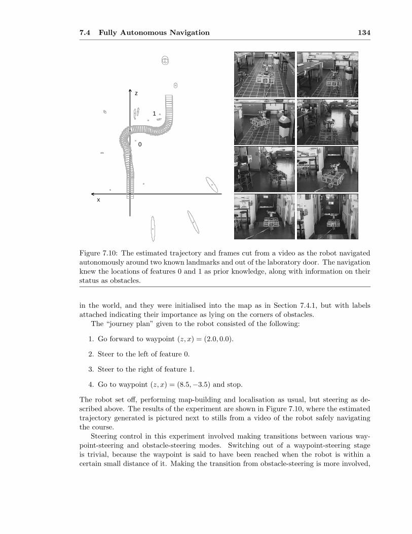
7.4 Fully Autonomous Navigation 134
x
z
0
1
Figure 7.10: The estimated trajectory and frames cut from a video as the robot navigatedautonomously around two known landmarks and out of the laboratory door. The navigationknew the locations of features 0 and 1 as prior knowledge, along with information on theirstatus as obstacles.
in the world, and they were initialised into the map as in Section 7.4.1, but with labelsattached indicating their importance as lying on the corners of obstacles.
The “journey plan” given to the robot consisted of the following:
1. Go forward to waypoint (z, x) = (2.0, 0.0).
2. Steer to the left of feature 0.
3. Steer to the right of feature 1.
4. Go to waypoint (z, x) = (8.5,−3.5) and stop.
The robot set off, performing map-building and localisation as usual, but steering as de-scribed above. The results of the experiment are shown in Figure 7.10, where the estimatedtrajectory generated is pictured next to stills from a video of the robot safely navigatingthe course.
Steering control in this experiment involved making transitions between various way-point-steering and obstacle-steering modes. Switching out of a waypoint-steering stageis trivial, because the waypoint is said to have been reached when the robot is within acertain small distance of it. Making the transition from obstacle-steering is more involved,

7.4 Fully Autonomous Navigation 135
but necessary to stop the robot from continuing in a never-ending orbit. The point atwhich to leave depends on what the robot is going to do next — some obstacles will causethe robot to deflect its trajectory only slightly in a short period of avoidance, while some,such as the inside corner of a 90◦ turn in a corridor, will require relatively long steeringmanoeuvres. The solution is to consider the next guidance point in the motion — eitherwaypoint or obstacle — and compare the current steering action with that which the nextpoint would be demanding in the absence of the current obstacle. The transition to thenext guidance point should be made when the two instantaneously agree: the current pointwill have done its job and control can pass to the next. This will only happen when thecurrent obstacle has been cleared sufficiently that the robot can start making for the nextwaypoint or obstacle-avoidance without danger of hitting it. Figure 7.10 shows the smoothtransitions occurring between waypoint and obstacle steering modes which this criterionproduces.
Note that in this experiment, steering around the known obstacles took place on apositional basis. The robot steered so as to avoid the known obstacles based on its currentposition estimate, even before it had first measured them. The automatic feature-selectioncriterion decided when it was necessary actually to measure the known features, and inthe experiments this proved to be as soon as they became visible, in order to lock therobot position estimate down to the world frame. The point when a first measurement ofknown feature 0 is made can be clearly seen in Figure 7.10 as a small kink in the robottrajectory: actually measuring the feature corrected the robot’s drifting position estimateand meant that the steering angle was changed slightly to correct the approach. Afterthis, the obstacle feature was fixated on only when it again became the best measurementto make. Otherwise, attention was paid to improving the map of automatically-acquiredfeatures.
Steering Around Closely-Spaced Obstacles
In a very similar experiment, the robot steered a course around two boxes acting as obstaclesin known positions. The journey commands this time were:
1. Steer to the left of feature 0.
2. Steer to the right of feature 1.
3. Go to waypoint (z, x) = (6.0, 0) and stop.
The results are shown in Figure 7.11. The safe radius R by which obstacles were to beavoided was set to a value 0.6m which is sufficient for the side of the robot to clear themwith some 20cm to spare.
7.4.4 Conclusion
The last section has shown with initial experiments how context-based steering controlcan be combined with map-building and position-based movement, and we feel that this isthe way forward for autonomous robots performing tasks in partially-known or unknownenvironments. Clearly it is not ideal to need to specify fully known landmarks and obstacles
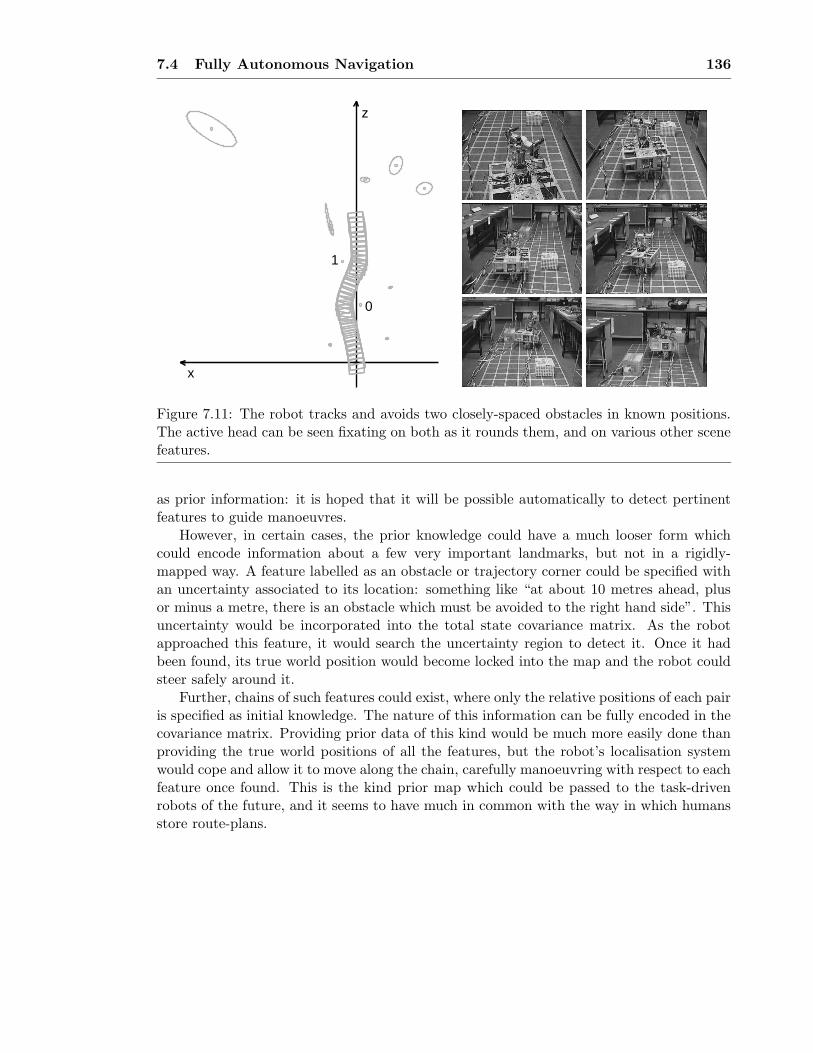
7.4 Fully Autonomous Navigation 136
x
0
1
z
Figure 7.11: The robot tracks and avoids two closely-spaced obstacles in known positions.The active head can be seen fixating on both as it rounds them, and on various other scenefeatures.
as prior information: it is hoped that it will be possible automatically to detect pertinentfeatures to guide manoeuvres.
However, in certain cases, the prior knowledge could have a much looser form whichcould encode information about a few very important landmarks, but not in a rigidly-mapped way. A feature labelled as an obstacle or trajectory corner could be specified withan uncertainty associated to its location: something like “at about 10 metres ahead, plusor minus a metre, there is an obstacle which must be avoided to the right hand side”. Thisuncertainty would be incorporated into the total state covariance matrix. As the robotapproached this feature, it would search the uncertainty region to detect it. Once it hadbeen found, its true world position would become locked into the map and the robot couldsteer safely around it.
Further, chains of such features could exist, where only the relative positions of each pairis specified as initial knowledge. The nature of this information can be fully encoded in thecovariance matrix. Providing prior data of this kind would be much more easily done thanproviding the true world positions of all the features, but the robot’s localisation systemwould cope and allow it to move along the chain, carefully manoeuvring with respect to eachfeature once found. This is the kind prior map which could be passed to the task-drivenrobots of the future, and it seems to have much in common with the way in which humansstore route-plans.

8Conclusions
In one of the first real implementations of navigation using active vision, we have shownthat it has a large part to play in the future of autonomous mobile robotics. To concludethis thesis, we will review what it is felt are the main contributions made, and discuss plansfor future related work.
8.1 Contributions
The main achievements of this thesis can be outlined as follows:
• An accurate, reliable and consistent algorithm for simultaneous localisation and map-building in unknown environments, using information from measurements of arbitraryfeatures and robot odometry (Chapter 5). The Kalman Filter-based method presentedis applicable to many systems, active and passive. The choice of a full-covariance ap-proach has proven its worth for extended periods of navigation, providing in particularthe capability to re-measure features after a period of neglect and recover accurateposition estimation after periods of drift.
• Good mathematical modelling of vehicle and active head (Chapter 3). These modelsallowed the system to operate accurately, and included consideration of the uncer-tainties introduced by the hardware.
• A full robot implementation of the techniques presented for active visual navigation(Chapters 4, 5). Provision of capabilities such as correlation search ellipses, continuousfixated feature tracking and dynamic steering control have allowed ideas to be testedin realistic circumstances.

8.2 Future Work 138
• Extended and carefully performed experiments in a real environment (Chapters 5, 6,7). Meaningful experiments were carried out into most aspects of the work, using therobot in a realistic setting with ground-truth comparisons available from an accurategrid.
• An efficient algorithm for updating the Kalman Filter in the case of extended periodsof single-feature tracking (Chapter 6). A rearrangement of the bookkeeping of filteringallows updates to be carried out in constant time independent of the number of featuresin the full map, while information is retained to enable a full unapproximated mapupdate when processing time becomes available.
• An automated strategy for selective fixation on scene features (Chapter 6). Theactive head is used to best effect to make the feature measurements which do most toimprove the quality of map and localisation estimations. The effects of finite activehead performance have also been investigated.
• An approach to automatic map maintenance (Chapter 7). Criteria are presented asa basis for deciding when to delete or add features from or to a self-generated map,with the goal of maintaining it in a globally useful and consistent form.
• Experiments in goal-directed navigation (Chapter 7). With the aim of producing amobile robot which could perform useful tasks, using prior information where avail-able, methods such as incorporating known features into an automatically generatedmap and steering compound paths through waypoints and around obstacles have beensuccessfully implemented.
8.2 Future Work
The framework put in place by the work in this thesis gives a strong basis for severalinteresting directions of future work, which will lead to increasing levels of autonomy formobile robots in useful applications. We feel that work should be concentrated on two mainareas:
• The clear benefits demonstrated in this thesis of a full-covariance approach to simulta-neous localisation and map-building (Chapter 5) are balanced by the computationalcomplexity of maintaining a map of this form. It is felt that it will be possible toextend the algorithm of Section 6.2, which provides efficient updates for the case ofrepeated measurements of one feature, to the situation where a certain subset of thetotal number of features in the map can be kept up to date in real time, while the restcan be updated in one computationally-expensive step when this becomes necessary.
Full knowledge of the covariances between a certain set of features permits the feature-selection strategies of Section 6.3 to operate and make choices between them. In aparticular robot situation, it will only be possible to make measurements of a certainnumber of features at a given time. If the states and covariances relating these arekept up to date in real time, feature selection can take place as required. It is notnecessary, though, to have real-time information about the features which are notmeasurable. It is hoped that the instructions about how to generically update these

when the time comes will be able to be stored “on the back burner” for a full updateto occur when necessary.
This would remove limits (aside from storage space) on the size of global featuremaps which could be maintained. For example, an indoor robot moving betweenrooms would only need to keep real-time information on those features within thecurrent room. When a different room was entered, the robot could stop briefly toperform the full map update step and bring its estimates about the features there upto date.
If successfully formulated, this method could have large benefits in many areas, es-pecially in the structure from motion community in computer vision research, wheresequential updating of structure and motion estimates has now frequently been aban-doned due to the problems of motion drift in favour of batch approaches, which cannotproduce maps in real-time.
Further gains in efficiency could be gained by potentially making approximationsabout the full covariance matrix. As discussed Section 5.2, it may not be necessary tomaintain covariance links between features which are distantly separated in the map(not necessarily in terms of pure distance, but the number of measurements involvedin estimating their relative locations). The full covariance matrix P would tend tobecome more diagonal.
• The other main area of future research is more focussed on the problem of active visualnavigation. Truly autonomous robots need the capability to detect obstacles and freespace, and react by adjusting their movements on the way to a global goal. Free-spacerepresentations must be incorporated with the landmark feature map, perhaps witha local dense map for obstacle avoidance, and large-scale features fully incorporatedwith the landmarks. The use of features other than points, such as lines or planes, inthe map-building approach will be considered.
The idea of contextual navigation will also be investigated further. Automaticallyattaching labels to map features indicating their status as obstacles will allow the robotto use the steering method already implemented in Chapter 7 to perform avoidanceand plan safe paths.
139
Bibliography
[1] M. Armstrong, A. Zisserman, and R. Hartley. Self-calibration from image triplets.In B. Buxton and R. Cipolla, editors, Proceedings of the 4th European Conference on
Computer Vision, Cambridge, volume 1, pages 3–16, April 1996.
[2] N. Ayache. Artificial Vision for Mobile Robots: Stereo Vision and Multisensory Per-
ception. MIT Press, Cambridge MA, 1991.
[3] R. Bajcsy. Active perception. Proc.IEEE, 76(8):996–1005, 1988.
[4] D. H. Ballard and A. Ozcandarli. Eye fixation and kinetic depth. In Proceedings of
the 2nd International Conference on Computer Vision, Tampa, 1988.
[5] P. H. Batavia, D. A. Pomerleau, and C. E. Thorpe. Overtaking vehicle detection usingimplicit optical flow. In Proceedings of the IEEE Intelligent Transportation Systems
Conference, Boston, MA, 1997.
[6] P. A. Beardsley, I. D. Reid, A. Zisserman, and D. W. Murray. Active visual navigationusing non-metric structure. In Proceedings of the 5th International Conference on
Computer Vision, Boston, pages 58–65. IEEE Computer Society Press, 1995.
[7] P. A. Beardsley, A. Zisserman, and D. W. Murray. Navigation using affine structurefrom motion. In Proceedings of the 3rd European Conference on Computer Vision,
Stockholm, volume 2, pages 85–96, 1994.
[8] P. A. Beardsley, A. Zisserman, and D. W. Murray. Sequential update of projectiveand affine structure and motion. Technical Report OUEL report 2012/94, Dept. ofEngineering Science, University of Oxford, 1994.
[9] A. Blake, A. Zisserman, and R. Cipolla. Visual exploration of free-space. In A. Blakeand A. Yuille, editors, Active Vision. MIT Press, Cambridge, MA, 1992.
[10] J.-Y. Bouget and P. Perona. Visual navigation using a single camera. In ICCV5,pages 645–652, Los Alamitos, CA, 1995. IEEE Computer Society Press.
[11] K. J. Bradshaw, P. F. McLauchlan, I. D. Reid, and D. W. Murray. Saccade and pursuiton an active head/eye platform. Image and Vision Computing, 12(3):155–163, 1994.
[12] R. A. Brooks. A robust, layered control system for a mobile robot. Technical ReportA.I. Memo 864, Massachusetts Institute of Technology, September 1985.
[13] R. A. Brooks. Achieving artificial intelligence through building robots. TechnicalReport A.I. Memo 899, Massachusetts Institute of Technology, May 1986.

[14] R. A. Brooks. Intelligence without representation. In Workshop on the Foundations
of Artificial Intelligence, Dedham, MA, 1987.
[15] R. A. Brooks and L. A. Stein. Builing brains for bodies. Technical Report A.I. Memo1439, Massachusetts Institute of Technology, August 1993.
[16] C.M. Brown. Gaze control with interactions and delays. IEEE Trans. Sys. Man and
Cyb., 63:61–70, 1990.
[17] T. P. H. Burke. Design of a Modular Mobile Robot. PhD thesis, University of Oxford,1994.
[18] S. A. Cameron and P. J. Probert, editors. Advanced Guided Vehicles — Aspects of
the Oxford AGV Project. World Scientific, Singapore, 1994.
[19] J. F. Canny. Finding edges and lines in images. Master’s thesis, MIT, 1983.
[20] R. Cipolla and A. Blake. The dynamic analysis of apparent contours. In Proceedings
of the 3rd International Conference on Computer Vision, Osaka, 1990.
[21] J. C. Clarke. Applications of Sequence Geometry to Visual Motion. PhD thesis,University of Oxford, 1998.
[22] G. Cross and A. Zisserman. Quadric reconstruction from dual-space geometry. InProceedings of the 6th International Conference on Computer Vision, Bombay, pages25–31, 1998.
[23] M. Csorba, J. K. Uhlmann, and H. F. Durrant-Whyte. A new approach to simul-taneous localization and dynamic map building. In SPIE Proceedings, pages 26–36,1996.
[24] A. J. Davison, I. D. Reid, and D. W. Murray. The active camera as a projectivepointing device. In Proceedings of the 6th British Machine Vision Conference, Bir-
imingham, pages 453–462, 1995.
[25] L. de Agapito, D. Q. Huynh, and M. J. Brooks. Self-calibrating a stereo head: anerror analysis in the neighbourhood of degenerate configurations. In Proceedings of
the 6th International Conference on Computer Vision, Bombay, pages 747–753, 1998.
[26] F. Du. Navigation in tight clearances using active vision. Technical Report OUEL2041/94, Department of Engineering Science, University of Oxford, 1994. First yeartransfer report.
[27] H. F. Durrant-Whyte. Where am I? A tutorial on mobile vehicle localization. Indus-
trial Robot, 21(2):11–16, 1994.
[28] S.M. Fairley, I.D. Reid, and D.W. Murray. Transfer of fixation for an active stereoplatform via affine structure recovery. In Proceedings of the 5th International Confer-
ence on Computer Vision, Boston, pages 1100–1105, 1995.
141

[29] O. D. Faugeras. What can be seen in three dimensions with an uncalibrated stereorig? In G. Sandini, editor, Proceedings of the 2nd European Conference on Computer
Vision, Santa Margharita Ligure, Italy, pages 563–578. Springer-Verlag, 1992.
[30] O.D. Faugeras. Three-Dimensional Computer Vision. MIT Press, 1993.
[31] N.J. Ferrier. The harvard binocular head. Technical Report 91-9, Harvard RoboticsLaboratory, 1991.
[32] C. R. Gallistel. The Organisation of Learning. MIT Press, Cambridge MA, 1990.
[33] J. Gluckman and S. K. Nayar. Ego-motion and omnidirectional cameras. In Pro-
ceedings of the 6th International Conference on Computer Vision, Bombay, pages999–1005, 1998.
[34] M. Brady H. Wang and C. Bowman. Architectures and algorithms for 3D vision:the parallel Droid system. In S. Cameron and P. Probert, editors, Advanced Guided
Vehicles, pages 125–139. World Scientific, Singapore, 1994.
[35] C. G. Harris. Tracking with rigid models. In A. Blake and A. Yuille, editors, Active
Vision. MIT Press, Cambridge, MA, 1992.
[36] C. G. Harris and J. M. Pike. 3D positional integration from image sequences. In Proc.
3rd Alvey Vision Conference, Cambridge, pages 233–236, 1987.
[37] C. G. Harris and M. Stephens. A combined corner and edge detector. In Proc. 4th
Alvey Vision Conference, Manchester, pages 147–151, 1988.
[38] R.I. Hartley. In defence of the 8-point algorithm. In Proceedings of the 5th Interna-
tional Conference on Computer Vision, Boston, pages 1064–1070, 1995.
[39] R.I. Hartley, R. Gupta, and T. Chang. Stereo from uncalibrated cameras. In Pro-
ceedings of the IEEE Conference on Computer Vision and Pattern Recognition, pages761–764, 1992.
[40] J. J. Heuring. Applications of Computer Vision to Telepresence. PhD thesis, Univer-sity of Oxford, 1997.
[41] J. J. Heuring and D. W. Murray. Visual head tracking and slaving for visual telepres-ence. In Proceedings of the IEEE International Conference on Robotics and Automa-
tion, 1996.
[42] E. Huber and D. Kortenkamp. Using stereo vision to pursue moving agents with amobile robot. In IEEE International Conference on Robotics and Automation, May1995.
[43] E. Huber and D. Kortenkamp. A behavior-based approach to active stereo visionfor mobile robots. To appear in Engineering Applications of Artificial IntelligenceJournal, 1998.
[44] S. Hutchinson, G. D. Hager, and P. I. Corke. A tutorial on visual servo control. IEEE
Trans. Robotics and Automation, 12(5):651–669, 1996.
142

[45] M. Isard and A. Blake. Contour tracking by stochastic propagation of conditional den-sity. In Proceedings of the 4th European Conference on Computer Vision, Cambridge,pages 343–356, 1996.
[46] T. M. Jochem, D. A. Pomerleau, and C. E. Thorpe. Vision guided lane transition. InIEEE Symposium on Intelligent Road Vehicles, Detroit, MI, 1995.
[47] E. Krotkov, M. Hebert, and R. Simmons. Stereo perception and dead-reckoning for aprototype lunar rover. Autonomous Robots, 2(4):313–331, 1995.
[48] M. F. Land and J. Horwood. Which parts of the road guide steering? Nature,377:339–340, 1995.
[49] M. F. Land and D. N. Lee. Where we look when we steer. Nature, 369:742–744, 1994.
[50] D. Langer, J. K. Rosenblatt, and M. Hebert. A behaviour-based system for off-roadnavigation. IEEE Trans. Robotics and Automation, 10(6):776–782, 1994.
[51] D. Lee and M. Recce. Quantitative evaluation of the exploration strategy of a mo-bile robot. In AISB 94 Workshop: Models or behaviours — which way forward for
robotics?, University of Leeds, April 1994.
[52] J. J. Leonard. Directed Sonar Sensing for Mobile Robot Navigation. PhD thesis,University of Oxford, 1990.
[53] J. J. Leonard, H. Durrant-Whyte, and I. J. Cox. Dynamic map building for anautonomous mobile robot. International Journal of Robotics Research, 11(4):286–298, 1992.
[54] J. J. Leonard and H. F. Durrant-Whyte. Directed Sonar Navigation. Kluwer AcademicPress, 1992.
[55] F. Li. Active Stereo for AGV Navigation. PhD thesis, University of Oxford, 1996.
[56] H.C. Longuet-Higgins. A computer algorithm for reconstructing a scene from twoprojections. Nature, 293:133–135, 1981.
[57] J. Manyika. An Information-Theoretic Approach to Data Fusion and Sensor Manage-
ment. PhD thesis, University of Oxford, 1993.
[58] D. Marr. Vision. MIT Press, Cambridge MA, 1982.
[59] S. J. Maybank, A. D. Worrall, and G. D. Sullivan. Filter for car tracking based onacceleration and steering angle. In Proceedings of the 7th British Machine Vision
Conference, Edinburgh, pages 615–624, 1996.
[60] S.J. Maybank and O. Faugeras. A theory of self-calibration of a moving camera.International Journal of Computer Vision, 8(2):123–151, 1992.
[61] J. Mayhew, Y. Zhang, and S. Cornell. The adaptive control of a four-degrees-of-freedom stereo camera head. Phil. Trans. Royal Society London B, 337:315–326,1992.
143
[62] P. F. McLauchlan. Horatio: Libraries for vision applications. Technical Report OUEL1967/92, Dept. Engineering Science, University of Oxford, October 1992.
[63] P. F. McLauchlan and D. W. Murray. A unifying framework for structure and motionrecovery from image sequences. In Proceedings of the 5th International Conference on
Computer Vision, Boston. IEEE Computer Society Press, 1995.
[64] P.F. McLauchlan and D.W. Murray. Active camera calibration for a head-eye platformusing a variable state-dimension filter. Accepted for PAMI, 1994.
[65] H. Moravec. Obstacle avoidance and navigation in the real world by a seeing robotrover. Technical Report CMU-RI-TR-3, Carnegie-Mellon University, Robotics Insti-tute, September 1980.
[66] F. Mura and N. Franceschini. Obstacle avoidance in a terrestrial mobile robot providedwith a scanning retina. In Proceedings of the 1996 Intelligent Vehicles Symposium,pages 47–52, 1996.
[67] D. W. Murray, P. F. McLauchlan, I. D. Reid, and P. M. Sharkey. Reactions to periph-eral image motion using a head/eye platform. In Proceedings of the 4th International
Conference on Computer Vision, Berlin, pages 403–411, Los Alamitos, CA, 1993.IEEE Computer Society Press.
[68] D. W. Murray, I. D. Reid, and A. J. Davison. Steering and navigation behaviours usingfixation. In Proceedings of the 7th British Machine Vision Conference, Edinburgh,pages 635–644, 1996.
[69] U. Nehmzow. Animal and robot navigation. In The Biology and Technology of Intel-
ligent Autonomous Agents. Springer Verlag, 1993.
[70] K. Pahlavan, T. Uhlin, and J-O. Eklundh. Integrating primary ocular processes. InProceedings of the 2nd European Conference on Computer Vision, Santa Margharita
Ligure, Italy, pages 526–541, 1992.
[71] J. M. Pichon, C. Blanes, and N. Franceschini. Visual guidance of a mobile robotequipped with a network of self-motion sensors. In SPIE Conference on Mobile Robots
4, pages 44–53, 1990.
[72] D. Pomerleau. Neural Network Perception for Mobile Robot Guidance. Kluwer Aca-demic Publishers, 1993.
[73] P. Pritchett and A. Zisserman. Wide baseline stereo matching. In Proceedings of the
6th International Conference on Computer Vision, Bombay, pages 754–760, 1998.
[74] V. S. Ramachandran. Visual perception in people and machines. In A. Blake, editor,A.I. and the Eye, chapter 3. Wiley and Sons, 1990.
[75] I. D. Reid and P. A. Beardsley. Self alignment of a binocular robot. In Proceedings
of the 6th British Machine Vision Conference, Birimingham, pages 443–452, 1995.
144

[76] I. D. Reid and D. W. Murray. Tracking foveated corner clusters using affine structure.In Proceedings of the 4th International Conference on Computer Vision, Berlin, pages76–83, Los Alamitos, CA, 1993. IEEE Computer Society Press.
[77] I. D. Reid, D. W. Murray, and K. J. Bradshaw. Towards active exploration of staticand dynamic scene geometry. In IEEE International Conference on Robotics and
Automation, pages 718–723, San Diego, May 1994.
[78] S. Rougeaux and Y. Kuniyoshi. Robust real-time tracking on an active vision head.In Proceedings of the IEEE Conference on Computer Vision and Pattern Recognition,1997.
[79] S. M. Rowe and A. Blake. Statistical background modelling for tracking with a virtualcamera. In Proceedings of the 6th British Machine Vision Conference, Birimingham,1995.
[80] W. Rucklidge. Efficient guaranteed search for gray-level patterns. In Proceedings of
the IEEE Conference on Computer Vision and Pattern Recognition, pages 717–723,1997.
[81] S. Scheding, G. Dissanayake, E. M. Nebot, and H. F. Durrant-Whyte. Slip modellingand aided inertial navigation of an LHD. In Proceedings of the IEEE International
Conference on Robotics and Automation, pages 1904–1909, 1997.
[82] S. Scheding, E. M. Nebot, M. Stevens, H. F. Durrant-Whyte, J. Roberts, P. Corke,J. Cunningham, and B. Cook. Experiments in autonomous underground guidance.In Proceedings of the IEEE International Conference on Robotics and Automation,pages 1898–1903, 1997.
[83] C. Schmid and A. Zisserman. Automatic line matching across views. In Proceedings of
the IEEE Conference on Computer Vision and Pattern Recognition, pages 666–672,1997.
[84] P. M. Sharkey, D. W. Murray, S. Vandevelde, I. D. Reid, and P. F. McLauchlan. Amodular head/eye platform for real-time reactive vision. Mechatronics, 3(4):517–535,1993.
[85] J. Shi and C. Tomasi. Good features to track. In Proceedings of the IEEE Conference
on Computer Vision and Pattern Recognition, pages 593–600, 1994.
[86] E. Shilat, M. Werman, and Y. Gdalyahu. Ridge’s corner detection and correspondence.In Proceedings of the IEEE Conference on Computer Vision and Pattern Recognition,pages 976–982, 1997.
[87] S. Smith. A new class of corner finder. In Proceedings of the 3rd British Machine
Vision Conference, Leeds, pages 139–148, 1992.
[88] A. Stevens, M. Stevens, and H. F. Durrant-Whyte. OxNav: Reliable autonomousnavigation. In Proceedings of the IEEE International Conference on Robotics and
Automation, pages 2607–2612, 1995.
145
[89] H. W. Stone. Mars pathfinder microrover: A low-cost, low-power spacecraft. InProceedings of the 1996 AIAA Forum on Advanced Developments in Space Robotics,
Madison, WI., 1996.
[90] P. Sturm. Critical motion sequences for monocular self-calibration and uncalibratedeuclidean reconstruction. In Proceedings of the IEEE Conference on Computer Vision
and Pattern Recognition, pages 1100–1105, 1997.
[91] J. I. Thomas, A. Hanson, and J. Oliensis. Understanding noise: The critical role ofmotion error in scene reconstruction. In Proceedings of the 4th International Confer-
ence on Computer Vision, Berlin, 1993.
[92] J. I. Thomas, A. Hanson, and J. Oliensis. Refining 3D reconstructions: A theoreticaland experimental study of the effect of cross-correlation. Computer Vision, Graphics,
and Image Processing, 60(3):359–370, 1994.
[93] J. I. Thomas and J. Oliensis. Automatic position estimation of a mobile robot. InIEEE Conference on AI Applications, pages 438–444, 1993.
[94] C. Tomasi and T. Kanade. Shape and motion from image streams under orthography:A factorization approach. International Journal of Computer Vision, 9(2):137–154,1992.
[95] P. H. S. Torr, A. W. Fitzgibbon, and A. Zisserman. Maintaining multiple motionmodel hypotheses over many views to recover matching and structure. In Proceedings
of the 6th International Conference on Computer Vision, Bombay, pages 485–491,1998.
[96] P. H. S. Torr and A. Zisserman. Robust computation and parameterization of mul-tiple view relations. In Proceedings of the 6th International Conference on Computer
Vision, Bombay, pages 727–732, 1998.
[97] R Y Tsai and T S Huang. Uniqueness and estimation of three-dimensional motionparameters of rigid objects with curved surfaces. IEEE Transactions on Pattern
Analysis and Machine Intelligence, PAMI-6:13–27, 1984.
[98] H. Wang and J. M. Brady. Corner detection for 3D vision using array processors. InProc. BARNAIMAGE-91, Barcelona. Springer-Verlag, 1991.
[99] J. Weng, T. S. Huang, and N. Ahuja. Motion and structure from two perspectiveviews: Algorithms, error analysis and error estimation. IEEE Transactions on Pattern
Analysis and Machine Intelligence, 11(5):451–476, 1989.
[100] P. Whaite and F. P. Ferrie. Autonomous exploration: Driven by uncertainty. IEEE
Transactions on Pattern Analysis and Machine Intelligence, 19(3):193–205, 1997.
[101] C. S. Wiles, A. Maki, N. Matsuda, and M. Watanabe. Hyper-patches for 3D modelacquisition and tracking. In Proceedings of the IEEE Conference on Computer Vision
and Pattern Recognition, pages 1074–1080, 1997.
146

[102] C. Zeller and O. Faugeras. Applications of non-metric vision to some visual guidedtasks. Technical Report INRIA Rapport de recherche 2308, INRIA Sophia-Antipolis,1994.
[103] Z. Zhang and O. Faugeras. 3D Dynamic Scene Analysis. Springer-Verlag, 1992.
147