mnidirectional Gait

Generating Algorit for

Hexapo Robot

Michael Fielding

A thesis presented for the degree of

Doctor of Philosophy

in

Mechanical Engineering

at the

University of Canterbury,

Christchurch, New Zealand.

18 June 2002

Abstract

vValking robots have long been proposed as solutions to the problem of

mobile machines operating in unstructured and natural environments be­

cause they can traverse relatively large obstacles and avoid dangerous or

sensitive areas of the ground. Walking machines that can move in any

direction and turn through any radius have an 'omnidirectional manoeu­

vring' capability. Hexapodal (six-legged) walking machines have advan­

tages over bipedal and quadrupedal machines in the areas of stability,

payload and simplicity, as well as the ability to operate with damaged or

broken

Walking robots inspired by insect neurology and biology continue to ex­

tend the state of the art, but using this 'biologically inspired' approach to

develop behaviours not exhibited by the animals requires further insight

into the principles of walking. Part of this thesis develops a possible ex­

planation for the distributed inter-leg influences that control walking in

the stick insect: that legs swing forward to take their next step when the

proximity of other legs or workspace boundaries restricts their movement.

This new concept, called the 'restrictedness' algorithm, has similarities to

distributed gait controllers in the literature but with enhanced capabilities

and simpler implementation. The restrictedness algorithm is a significant

contribution to the field of walking robotics and may also be of relevance

to future biological studies.

Omnidirectional walking requires the adaptation of leg movements to the

locomotion direction and robustness to unusual leg lifting positions. A

novel velocity field specified in a 'task coordinate system' for each . leg is

described, a scheme that allows simple realtime adaptation to different

commanded body movement vectors and changing spatial relationships

between the legs. Active compliance and automatic levelling improve the

robot's interaction with the ground, especially over rough ground.

Experiments with the robot Hamlet, designed and built primarily by the

iv ABSTRACT

author, proved that the new restrictedness and velocity field swing algo­

rithms display the important traits required from a walking robot gait

controller. Specifically, the algorithm provided delivers range of opti­

mal forward walking gaits observed in insects while also supporting ollmi­

directional walking, including rotating while simultaneously translating.

Optimization by simulating a model of the robot improved

forward walking performance.

controller's

Four papers were presented in the course of completing this work:

Fielding, Michael R., Dunlop, Reg and Damm'en, Christopher J., (2001).

Hamlet: Force/Position Controlled Hexapod 'Walker - Design and

tems. In Proc. Conference on Control Applications (CCA), Mexico

City, Mexico, p 984-989

Fielding, R. and Dunlop, Reg, (2001). Exponential Fields to

Establish Influences for Omnidirectional Hexapod Gait. In Proc.

4th Conference on Climbing and Walking Robots (CLAWAR), Karlsruhe,

Germany, 4, p 587-594

Fielding, Michael R., (2001). Hexapod Leg Control by Vector Fields &

Restriction Measures. In Proc. 8th New Zealand Engineering and Tech­

nology Postgraduate Conference, Hamilton, New Zealand, p 149-152

Fielding, Michael R., Dunlop, G. Reg (2002). Omnidirectional Hexapod

Walking and Efficient Gaits Using Restrictedness .. In Proc. 5th Con­

ference on Climbing and Walking Robots (CLAWAR), Paris, In

Press

The paper delivered at the 8th New Zealand Engineering and Technology

Postgraduate Conference won Overall Best Written Paper and Best Oral

Presentation prizes in the Electronics, Control and Computing section.

Acknowledgements

The following people and entities deserve and receive my unreserved

thanks:

Dr Reg Dunlop for supervision, guidance and advice throughout the many

phases of the project and the thesis, for encouraging me, and for a steady

stream of visitors whose interest motivated and enthused me. Also to Dr

Chris Damaren, my original supervisor, for setting me on the right track.

Julian Murphy, Ken Brown, Scott Amies, Andy Cree, Graham Harris and

Paul Welles of the Department of Mechanical Engineering technical staff

for their advice, expertise and direct involvement in various construction

phases.

Richard Barton for designing Hamlet's prototype

The University library for their top-class conventional and online re­

sources.

The University of Canterbury for funding the project and the Doctoral

Scholarship for which I am extremely grateful, the IEEE Southern Section

and the Christchurch Branch of the Royal Society of New Zealand for

conference funding.

Karen Healey and Erin Harrington for their invaluable proofreading.

Last, but not least, my family and friends for their unwavering encour­

agement and support.

If it were not for each of these people, you would not be reading this

today.

Contents

Abstract

Acknowledgements

1 Introduction 1.1 Applications and Motivation

1.1.1 Why Hexapods? ... 1.1.2 Biological Inspiration

1.2 Terminology......... 1.2.1 Spatial Terminology 1.2.2 Control Hierarchy .. 1.2.3 Gait Control Terminology

1.3 Review .............. . 1.3.1 Structurally-determined Gait 1.3.2 Fixed Gait ..... . 1.3.3 Endogenous Networks 1.3.4 Rule-based Free Gait. 1.3.5 Optimal Free Gait . . 1.3.6 Distributed Free Gait 1.3.7 Summary

1.4 Objectives. 1.5 Outline .....

2 Observations on Insect Locomotion 2.1 Insect Physiology ...

2.1.1 Body Parts . . . 2.1.2 Leg Structure . .

2.1.3 Neurophysiology 2.1.4 Leg Sensory Organs

2.1.5 Other Sensory Organs 2.1.6 Central Nervous System

2.2 Leg and Body Movement 2.2.1 Feedback Control. 2.2.2 Stance/Retraction

2.2.3 Swing/Protraction

iii

v

1 1 1

3 4

5 5 7 9

9

10

12 12 13 15 16 18

18

21 21 22 22 24 24

25 25 26

26 27

28

viii

2.2.4 Body ........ .

2.3 Gait Patterns and Selection 2.3.1 Basic Gait Model .. 2.3.2 Turning....... 2.3.3 Starting and Stopping 2.3.4 Obstacle Negotiation .

2.4 Coordinating Mechanisms .. 2.4.1 Statistical Correlation 2.4.2 Amputation and Deafferentation 2.4.3 Interference with Leg Movement 2.4.4 Summary .....

3 Experimental Equipment 3.1 Requirements.....

3.1.1 Autonomy ... 3.1.2 Environmental 3.1.3 Miscellaneous.

3.2 Hardware Description 3.2.1 Hamlet .... 3.2.2 Fixed Electronics . 3.2.3 Experimental Environment

3.3 Dataflow..... 3.4 Conclusions....

3.4.1 Problems . 3.4.2 Capabilities

4 Gait Patterns and Selection 4.1 Introduction ........ .

4.1.1 Observations, Implementation) Principles 4.1.2 Hierarchy.............. 4.1.3 Anterior and Posterior . . . . . . .

4.2 Interpretation of Biological Observations . 4.2.1 Stability Rules ....... . 4.2.2 Limitation of Leg Restriction 4.2.3 Gait Pattern Convergence 4.2.4 Basic Algorithm .....

4.3 Restrictedness........... 4.3.1 Measuring Restrictedness 4.3.2 Parameters Determining Restrictedness 4.3.3 Mode Dependence . . . . . . . . .

4.4 Implementation Details ......... . 4.4.1 Increasing Restrictedness Required 4.4.2 Halting When Overrestricted . . . 4.4.3 Halting and Increasing Restrictedness 4.4.4 Swing Priority ............ .

CONTENTS

28 29 29 32 33 33 33 34 34 36 38

41 41 41 43 43 44 44 47 47 47 49 49 50

53 53 53 55

56

56

56

57 58 58 60

60

61 64

65 65 67 68 70

CONTENTS ix

4.5 Experimental Results. . 70 4.5.1 Forward Walking 70 4.5.2 Manoeuvring 72

4.5.3 Discussion . . 76 4.6 Conclusions ~ .. . . . 77

4.6.1 Relationship to Biological Observations 78 4.6.2 Stability ..... ••••• + ........ 78

5 Leg and Body Movement 81

5.1 Introduction ....... 81 5.1.1 Stepping efficiency 82

5.2 Non-locomotive Movement. 83 5.2.1 Body Attitude Feedback . 83 5.2.2 Maintaining Ground Contact 85 5.2.3 Active Compliance 87 5.2.4 Summary ..... 89

5.3 Task Coordinate System 91 5.3.1 Introduction · . 91 5.3.2 Definition of Coordinate System 92 5.3.3 Anterior and Posterior . . . . . . . . . 93 5.3.4 Converting to and from Task Coordinate System 94

5.4 Stance Movement . . 94 5.4.1 Introd uction · ..... 94 5.4.2 Locomotion . . . . . . . 95 5.4.3 Ideal Stance Movement 95

5.5 Swing Movement .. 96 5.5.1 Introduction · ... 96 5.5.2 Control of x' · ... 98 5.5.3 Control of y' and Zl 98 5.5.4 Field Normalization 99 5.5.5 Field Design ...... 101 5.5.6 Step Length Reduction 103 5.5.7 Restrictedness During Swing 104 5.5.8 Predicted Restrictedness During Swing. 105 5.5.9 Calculating Step Length from Normalized Position 107 5.5.10 Summary .... 108 5.5.11 Discussion . ... 108

5.6 Swing/Stance Blending 112

5.6.1 Introduction · . 112

5.6.2 Blending Functions . 112

5.6.3 Restrictedness During Blending . 114

x

6 Modelling Restrictedness

6.1 Introduction ....

6.1.1 Motivation .. .

6.1.2 Review .... .

6.2 Basic Three Leg Restrictedness Model 6.2.1 Model Description .

6.2.2 Simulation Process . . . . . .

6.3 Stable B3RLM Parameters .....

6.3.1 Conditions For Convergence.

6.3.2 Valid Parameter Ranges ...

6.3.3 Effect of (3 on Convergence . 6.3.4 Valid Parameter Combinations

6.4 Optimal B3LRM Parameters .

6.4.1 Optimization Function. 6.4.2 Coarse Optimization

6.4.3 Fine Optimization 6.5 Conclusions

CONTENTS

115 115 115 117 118 118 120

121

123

123 126

127

127 127 128

131

133

7 Conclusions 135

7.1 Algorithm Summary . . . . . . . . . . . . . . . . . . 135 7.1.1 Merging Attitude Control and Restrictedness 136

7.1.2 Dataflow ..... 136 7.1.3 Energy Efficiency. 137

7.2 Summary . . . . . . . . .

7.2.1 Work Completed .

7.2.2 Capabilities and Advantages 7.3 Further Work . . . . . . .

7.3.1 Minor Extensions .. . 7.3.2 Major Extensions .. . 7.3.3 System Improvements

A Quick Definition Reference

B Hamlet

B.1 Mechanical

B.1.1 Chassis

B.1.2 Legs ..

B.1.3 Foot Force Sensors B.1.4 Protective Boots

B.2 Electronic . . . . . . . .

B.2.1 Leg I/O Modules

B.2.2 Serial Link . . .

B.2.3 Base Electronics . B.3 Software. . . . . . . . .

B.3.1 Basic Functions.

139 139 140

143

143 145 147

149

153

153

153

153

155

156

156

156

157

158 159

159

CONTENTS xi

B.3.2 User Interface ..... . 161

C Walking Algorithm Parameters 165 C.1 Restrictedness paJ'ameter Specification 165

C.2 Compliance Gains 166 C.3 Vector Field Design 167

Miscellaneous Equations 169

D.1 Swing Restrictedness Prediction . 169 D.2 Ideal stance trajectory . . . . 170

E Additional Modelling Results 171

References 177

List of Figures

1.1

1.2

Definitions of directions and terms indicating relative position 5

Generic walking robot control hierarchy

1.3 Leg movement phases

6

9

1.4 Dante II . 10

1.5 Genghis 11

1.6 ASV.. 11

1.7 MECANT. 13

1.8 Ambler .. 13

1.9 TUM walking machine 15

1.10 Lauron III . 15

1.11 Robot II . . 16

2.1 Major insect body parts of the weta, Hemideina thoracica 22

2.2 Typical insect leg. . . . . . . . 23

2.3 Wilson (1966)'s gait hypothesis 30

2.4 Diagonal stepping ....... 31

2.5 Diagonal stepping handedness. 31

3.1 Major hardware components of the robot Hamlet 44

3.2 Photo of Hamlet from front left quarter . . . . 45

3.3 a-joint locations and leg numbering for Hamlet 46

3.4 The location and action of the f3 joint spring. 46

3.5 Major parts and joint axes of Hamlet's legs

3.6 Dataflow diagram of the experimental hardware.

46

48

xiv LIST OF FIGURES

4.1 Layering of behaviour, implementation and principles. 54

4.2 Lifting any adjacent legs may violate static stability 57

4.3 Restrictedness measurements used on Hamlet . . . 62

4.4 Linear scaling of stance movements when R X -----+ 1 . 67

4.5 Gait diagram for tripod gait experiment . . 71

4.6 Position vs. time for tripod gait experiment 71

4.7 Photo of asymmetric starting configuration 72

4.8 Gait diagram for asymmetric starting configuration. 72

4.9 Curve walking photographic sequence 73

4.10 Gait diagram for curve walking experiment

4.11 Omnidirectional walking photographic sequence .

4.12 Gait diagram for turn-on-the-spot experiment ..

4.13 Potential instability using simple inhibition rules

5.1 Passing through Xi,home leads to longer steps.

5.2 Movement axes shared between controllers ...

5.3 Lowering behaviour contact hysteresis function

5.4 Demonstration of active compliance with Hamlet

5.5 Combined behaviour of non-locomotive movements

5.6 Foot velocities relative to the ground . . . .

5.7 Definition of the task coordinate system a'i.

5.8 Phases and general shape of the swing movement

5.9 Convergence of foot position to x* = o. . . . . . .

74

75

76

78

82

83

87

90

90

91

92

97

99

5.10 Relationship between a'i and swing-normalized position 100

5.11 Vector fields used for swing controller 102

5.12 Total swing field . . . . . . . . . . . . 103

5.13 Key components R X during a swing movement 105

5.14 Effect of R~Tedicted,swing functions on step length continuity 106

5.15 Step length reduction when swing is restricted. 107

5.16 Summary of the swing algorithm . . . 109

5.17 Convergence to x' = 0 during turning.

5.18 Simple swing blending functions

110

113

LIST OF FIGURES

5.19 Blending stance and swing movements .

6.1 Explanation of parameters for B3LRM .

xv

113

119

6.2 B3LRM simulation showing over-restricted movement 120

6.3 Block diagram of simulation process . 122

6.4 B3LRM parameters' influence, f3 = 0.5 124

6.5 Optimal parameter combinations for f3 0.75 129

6.6 Fine search for optimal parameter combinations for f3 = 0.75132

7.1 Dataflow diagram of full restrictedness controller

7.2 Gait transition with extra convergence influence.

7.3 Leg support when walking on slopes ...... .

138

144

A.1 Directions and terms indicating relative position 151

A.2 Leg movement phases ............... 151

B.1 Chassis and leg attachments . 153

B.2 Chassis cross-section . . 154

B.3 Leg design and features 154

B.4 Exploded diagram of motor/gear Oldham coupling 155

E.5 Foot force seIlSor design 156

B.6 Protective boots .... 156

B.7 Hamlet's leg I/O modules 157

B.8 Hamlet's serial link protocol. 158

E.9 Hamlet's DSP configuration 159

E.IO HAM control . 162

B.ll HAMdatafind 162

B.12 HAMviewer 163

B.13 HAMlogger 163

E.1 B3LRM parameters' influence, f3 = .5 172

B3LRM parameters' influence, f3 .95 173

E.3 Optimal parameter combinations for f3 = .5 174

E.4 Optimal parameter combinations for f3 .95 175

CHAPTER

Introduction

This chapter examines the applications for walking robots and the moti­

vation for choosing six-legged robots in particular. The field of biologically

inspired robotics is introduced in the first section and the second section

describes some terminology. The third section, a review of the recent lit­

erature in the field of gait controllers for many-legged walking robots, is

followed by the final sections explaining the research objectives and pro­

viding an outline of the thesis.

1.1 Applications and Motivation

This section examines why hexapod walking robots are being developed

and the reasons for investigating biological systems as inspiration for

robotics.

1.1 Why Hexapods?

One of the motivating factors often given for pursuing the development

of legged vehicles is that they can climb over larger obstacles than the

equivalent sized wheeled or tracked vehicle. This is indeed true, but wheels

and tracks can often be made larger if necessary and have the advantage

of being considerably simpler than legs. However, legged vehicles have

Advantage of legs

Omnidirectional manoeuvring

Choosing footfalls

Stability

Leg utilization

2 CHAPTER 1 INTRODUCTION

a definite advantage operating in confined spaces on irregular substrates

it is not possible to use a larger machine, or to transport one there.

Examples of environments where legged vehicles might be preferable to

wheeled ones include caves, ravines, mines, forests, buildings and other

planets.

One of the key advantages walking robots have over wheeled and espe­

cially tracked ones is that they can potentially move in any direction and

turn in any (even zero or negative) radius, a so-called 'omnidirectional ma­

noeuvring' capability. This is an essential capability in confined spaces,

yet surprisingly little research effort has been devoted to developing stable

and yet flexible controllers to achieve it.

Another important advantage is the legged robot's ability to choose its

footfalls rather than leaving tracks of its continuous contact with the

ground. Sensitive environments would certainly benefit from this, and

the robot may also be able to avoid stepping on dangerous parts of the

ground like holes, chemicals, damaged stairs or land mines. Using such

'precision stepping', walking robots potentially

unsafe footholds when climbing or descending

the ability to avoid

slopes, something that

a tracked or wheeled robot could not do. They could also increase their

width for stability but decrease it to navigate through doorways or other

narrow gaps.

These advantages are shared by walking robots regardless of the num­

ber of legs they have. However, hexapod robots, and those with more

than six legs, are 'statically stable' whereas bipeds and (to some extent)

quadrupeds are not. Static stability is the ability to remain standing with­

out continuously changing control input, and is achieved by maintaining

a tripod of legs supporting the body. Without static stability robots must

be dynamically stable or they will fall over. Dynamic stability is an active

area of research but one which has so far not shown sufficient robustness

for practical applications. Lower animals (such &'3 insects and some rep­

tiles) only use statically stable gaits, whereas higher animals (such as

mammals) can also use dynamically stab Ie Thus good statically

stable walking is the initial research goal. .

Quadrupeds can be statically stable if every leg spends at leasti of its

time on the ground, but this constrains the leg velocity when support­

ing the robot to a third or less of its rate when swinging forward for

the next step. Quadruped static walking speed is therefore limited to a

third of the actuator's actual limit. On other hand, if legs move in

both directions with equal velocity then they spend approximately half

1.1 APPLICATIONS AND MOTIVATION 3

their time supporting the robot. Static stability requires three legs on the

ground, so having six legs allows static stability with maximal leg utiliza­

tion. The stability margin (a measure of the safety of statically stable

walking) is also much smaller for statically walking quadrupeds than for

hexapods (Song and Waldron, 1987). Additional legs, for example eight

or ten, can improve stability at high speeds, but only by increasing the

already-positive stability margin.

The option of maintaining more than three legs on the ground allows

hexapods the ability to trade off speed for security in the expectation

of a foothold giving way. Having more supporting legs than bipeds or

quadrupeds also potentially allows hexapods to carry more weight. Any

increase in payload is desirable, particularly with current actuator tech­

nology, although the weight of the additional legs certainly offsets this

advantage to some degree. For autonomous missions in demanding envi­

ronments hexapods also have the potential ability to operate with dam­

aged or incapacitated legs, something that insects do with apparent ease

but which bipeds and statically walking quadrupeds could never do.

1.1.2 Biological Inspiration

Biological inspired robotics is the field of robotics in which parts of the

robot's control system or physical form are in some way derived from

observations of biological systems. Animals are the primary biological

inspiration in robotics research. Animals are the result of (depending

on your point of view) either a billion years of evolutionary design or

the unquestionable engineering capabilities of a supreme being. They are

justifiably expected to be 'best-practice' examples of adaptation to the

complex, natural environment that robots would ideally operate in. The

motivation behind learning from biology was summed up by Beer et al.

(1997): "Even the lowly cockroach can outperform the most sophisticated

autonomous robot at nearly every turn."

There are many levels to which biological inspiration can be taken. The

wheel has been the locomotive machine of choice for millennia, so at the

most cursory level the very idea of legged machines is biologically inspired.

At the extreme opposite end of the continuum is the challenging prospect

of completely mimicking a particular species in form and function. There

are a number of intermediate approaches that have been used in various

combinations:

If> assume that the physical structure of a paJ:ticular species is optimal

Extra advantages

Definition and motivation

Degrees of IIllmicry

"TVhile nature's way may

not be the only way, or

even necessarily the best

way, time and again we

have found unexpected ben­

efits from paying close at­

tention to the design of bi­

ological systems."

Beer et al. (1997)

4 CHAPTER 1 INTRODUCTION

for its ecological niche, and therefore mimic that entire design for a

robot with apparently similar mission requirements;

model just a part of the robot (e.g. the

particular species;

or chassis) on that of a

• develop novel sensory technology inspired by animal sensors and

investigate how it alters the robot's perception, and therefore its

ability to interact with its environment;

• observe animals and implement the same behaviour in robots faced

with the same situation, but using traditional engineering technolo­

gies;

• copy the exact neural organization of an animal to give the robot

the exact same capabilities;

• use adaptive technologies based on fundamental biological systems

(neural networks, genetic algorithms) and evolve a robot behaviour

or structure using reinforcement;

• attempt to find principles underlying behaviour or structure in bi­

ological systems, then use those principles to develop new problem

solutions.

The last approach holds the most promise for developing engineering so-

lutions but potentially requires greatest effort, or at least the most

insight. By examining and understanding the principles of why organisms

behave or grow as they do, could build new machines having

'organic-like' properties hitherto unseen in the natural world. This lacst

approach is the one adopted in this work

1.2 Terminology

The field of biologically inspired walking robots combines the lexicons of

robotics and biology. This section covers the important terms used in

this thesis. The first subsection explains some of the relevant biological

terms used in later sections. The second subsection defines a generic

control hierarchy for walking robots and explains what a gait controller

is and what its roles and responsibilities are. The section concludes by

explaining the terminology of

1.2 TERMINOLOGY 5

Caudal Rostral ----.. ~

Figure 1.1 Definitions of directions and terms indicating relative position used in this thesis. In this diagram the robot movement is to the right as indicated by the thick arrow.

1.2.1 Spatial Terminology

Fig. 1.1 shows the definitions of the major longitudinal directions relative

to the robot movement. These terms will be used frequently in later

sections. In addition there are two terms not shown in Fig. 1.1:

Contralateral On the other side (e.g. the left front leg's contralateral

neighbour is the right front leg).

Ipsilateral On the same side (e.g. the left middle leg's ipsilateral neigh­

bours are the left front and left rear legs).

The definitions just introduced are repeated in a fold-out quick reference

section, Appendix A.

1.2.2 Control Hierarchy

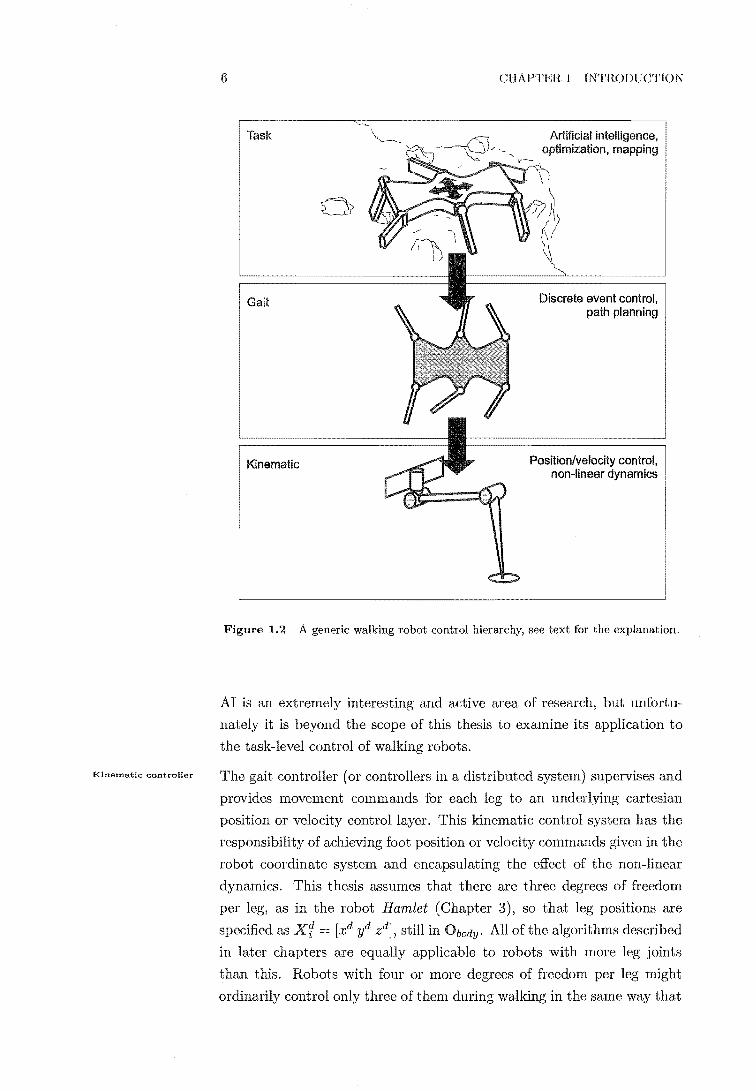
Fig. 1.2 shows a generic breakdown of the control hierarchy for walking

robots, a hierarchy that is almost universally accepted across the walking

robot and insect neurology communities. Lower levels have narrower scope

than higher levels but their actions are more specific.

task controller supervises the lower controller layers by providing

a desired direction, velocity and rotation in surface plane. In this

thesis these movements are specified in robot body coordinates Obody. Therefore the inputs to the next layer are a desired body translational

velocity Xtody = [xd il zdf and a desired body rotational velocity about

the robot's xyz axes ntodY [w~ w~ w~lT, where w~ indicates a rotational

velocity about the x axis etc.

The task controller may be a human operator as in Hamlet (the robot con­

structed for this work, see Chapter 3) or an 'artificial intelligence' (AI).

Direction definitions

Task controller

Kinematic controller

6

Task

Gait

Kinematic

CHAPTER 1 INTRODUCTIOK

Artificial intelligence, optimization, mapping

Discrete event control, path planning

Position/velocity control, non-linear dynamics

Figure 1.2 A generic walking robot control hierarchy, see text for the explanation.

AI is an extremely interesting and active area of research, but unfortu­

nately it is beyond the scope of this to examine its application to

the task-level control of walking robots.

The gait controller (or controllers in a distributed system) supervises and

provides movement commands for each leg to an underlying cartesian

position or velocity control layer. kinematic control system has the

responsibility of achieving foot position or velocity commands given in the

robot coordinate system and encapsulating the effect of the non-linear

dynamics. This thesis assumes that there are three degrees of freedom

per leg, as in the robot Hamlet (Chapter 3), so that leg positions are

specified as Xf = [.xd yd zd], still in Obody. All ofthe algorithms described

in later chapters are equally applicable to robots with more leg joints

than this. Robots with four or more degrees of freedom per leg might

ordinarily control only three of during walking in the same way that

1.2 TERMINOLOGY 7

insects do (c.f. §2.1.2). Robots with two degrees of freedom per leg cannot

realistically achieve omnidirectional walking anyway.

The fundanlental task of the gait control level is to translate short term

body movement commands from the task controller into leg trajectories

that achieve those commands. The gait of a robot or animal is the co­

ordinated leg and body movements that move the robot or animal from

one place to a different goal position. Specifically, the gait controller's

responsibilities include:

1. selecting which legs to lift and at what time to lift them;

2. planning coordinated trajectories for all the legs, either lifted or on

the ground;

3. selecting suitable footfalls (using kinematic and/or perceived envi­

ronmental constraints);

4. maintaining an appropriate body orientation and clearance with re­

spect to the ground;

5. managing the robot's weight distribution and foot force distribution

taking into account environmental and mechanical constraits;

6. reacting to changes in the environment's support capability (e.g.

slips, sinking).

The gait controller may be able to signal to the task controller that it

cannot achieve the intended movement, for example due to an impassable

obstacle. In this case a good task planner would attempt a different

movement. Note that, for a hexapod, the gait and kinematic levels are

required even by a human task planner because realistically a human

cannot coordinate all six limbs efficiently.

1.2.3 Gait Control Terminology

The gaits of statically stable animals walking over flat ground are· 'peri­

odic' and 'regular'. A gait is periodic if the legs always have the same

mode at the same point in their cycle and all the leg cycles are the same

length. Periodic gaits repeat the same sequence of steps every cycle. In

regular gaits, all the legs spend the same amount of time per cycle on the

ground (they have the same 'duty cycle', (3 = . The periodic

gait used by insects and many other animals is the 'wave gait' and its

Gait control

"A gait is a sequence of leg

motions coordinated with

a sequence of body mo­

tions for the purpose of

transporting the body of

the legged system from one

place to another."

Song and Waldron (1987)

Reversal of flow

Periodic gaits

Problems with tbem

" A free gait is an un-

restricted sequence of

steps [that]. .. enablers]

rock-hopping through ex­

tremely rough terrain and

the maneuvering required

to crawl through dense

obstacle fields. Free gaits

also smooth the transitions

from one gait pattern to

another'."

Wettergreen and Thorpe (1996)

Leg cycle definitions

8 CHAPTER 1 INTRODUCTION

derivatives, in which step waves move from the rear legs to the front, a

so-called 'metachronal' sequence. Song and Waldron (1987) proved that

metachronal wave gaits have optimal stability for forward walking, irre­

spective of the number of legs.

The following terms describe some common hexapodal stepping sequences.

In fact these are all wave gaits, although they do not always appear to be

§2.3 covers their relationship to the general wave gait.

Tripod gait A regular, periodic gait "with f3 = 0.5, where the anterior

and posterior legs on one side lift in time with the contralateral

middle leg, forming alternating tripods. This is a gait suitable for

high speed walking over relatively flat ground.

Tetrapod gait A metachronal wave gait where four are on the

ground all the time. Contralateral legs may in complete anti-

phase or at other phase relationships, but ipsilateral

in metachronal sequence.

always step

Crawl(ing) gait A very slow wave gait where only one leg lifts at a time.

A wave of steps travels forwards down one side, then the other.

One problem with periodic gaits is that they require synchronization be­

tween the expected and actual times that legs make contact with the

ground. Over uneven ground the time of footfall becomes unpredictable

(without very good perception), breaking the rigourously defined leg phas­

ing and compromising stability. Periodic gaits will be further disturbed

when the available footholds are limited and precision stepping is required.

Also with a periodic gait, direction changes have to wait until an

appropriate time in the cycle before they can be without desta-

bilizing the robot. In non-periodic gaits, so-called 'free gaits', there is

no predetermined stepping sequence. Algorithms or rules determine the

most appropriate stepping sequence as the situation requires it, maximiz­

ing stability and/or motion. Free gaits are more suitable than periodic

gaits when the movement command changes often, when walking over

rough ground, and when the application demands precision stepping.

Legs step in cycles with the major phases being called 'stance' or 'retrac­

tion' (when the leg is on the ground) and or 'protraction' (when

the leg is in the air) (Fig. 1.3). The terms stance and swing are gener­

ally used by roboticists, while biologists use retraction and protraction.

Roboticists also tend to use the word 'mode' in place of phase. Both sets

1.3 REVIEW 9

PEP AEP

Stance/Retraction

Figure 1.3 Relationship of leg movement phases and transition points. The arrow on the trajectory shows the direction of foot movement through the 'leg cycle', clockwise in this diagram.

of terms are used interchangeably in this thesis depending on the con­

text. The transition between the phases happens at the 'anterior extreme

position' (AEP) and 'posterior extreme position' (PEP). Sometimes the

swing part cycle is broken into three parts with its beginning and end

called 'lift' and 'extend' respectively. The middle part retains the name

swing. The particular meaning of swing is usually clear from the context.

1.3 Review

Many gait controllers have been inspired by insects and they exhibit

some very desirable properties (seamless transitions between gaits being

the most important), but most have never demonstrated omnidirectional

walking. Some other robots have been able to walk omnidirectionally, but

are exceedingly complex, slow, or don't display the desirable behaviours

of the biologically inspired controllers. Recently a few researchers have

begun to incorporate the best of both paradigms. This section reviews

the recent work (and relevant less recent work) on gait controllers for

multi-legged walking robots. Particular attention will be paid to their

omnidirectional walking capabilities.

1.3.1 Structurally-determined Gait

Robots with structurally-determined gait controllers are those where the

mechanical design dictates the leg movement pattern.

The simplest robots whose structure determines their gait are those with

two sets of three legs fixed to each other. For example, Wang et al. (1994)

constructed the Dual Tripod Walking Machine at Tsinghua University,

China, so that two tripods moved one with respect to each other in two

directions. The legs moved independently in the vertical direction but

Dual tripod machine

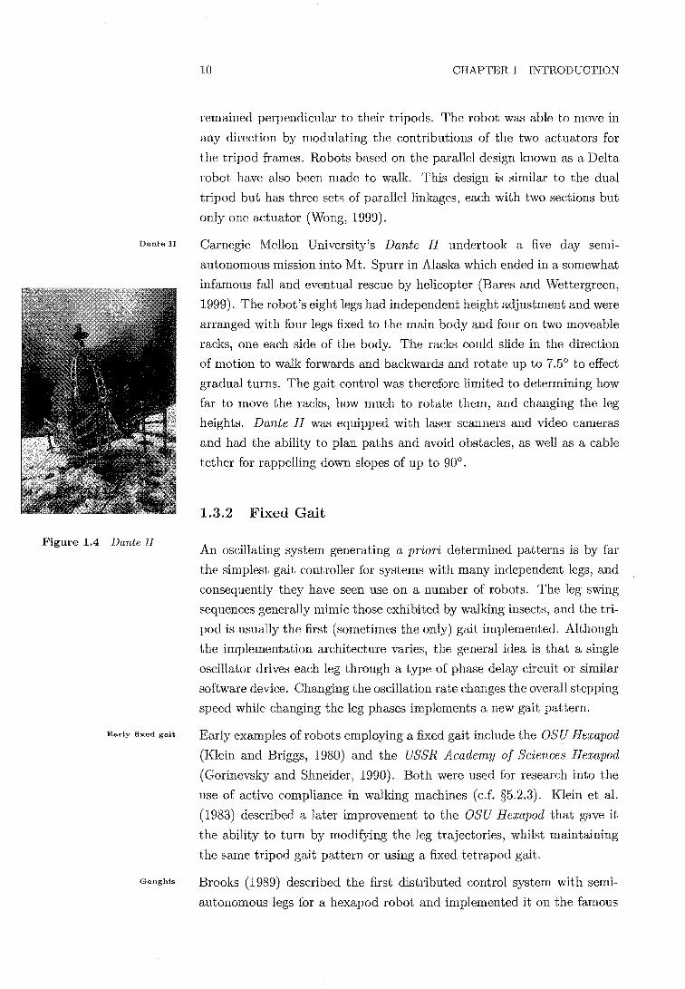
Dante II

Figure 1.4 Dante II

Early fixed gait

Genghis

10 CHAPTER 1 INTRODUCTION

remained perpendicular to their tripods. The robot was able to move in

any direction by modulating the contributions of the two actuators for

the tripod frames. Robots based on the parallel design known as a Delta

robot have also been made to walk. This design is similar to the dual

tripod but has three sets of parallel linkages, each with two sections but

only one actuator (Wong, 1999).

Carnegie Mellon University's Dante II undertook a five day

autonomous mission into Mt. Spurr in Alaska which ended in a somewhat

infamous fall and eventual rescue by helicopter (Bares and Wettergreen,

1999). The robot's eight legs had independent height adjustment and were

arranged with four legs fixed to the main body and four on two moveable

racks, one each side of the body. The racks could slide in the direction

of motion to walk forwards and backwards and rotate up to 7.50 to effect

gradual turns. The gait control was therefore limited to determining how

far to move the racks, how much to rotate them, and changing the leg

heights. Dante II was equipped with laser scanners and video cameras

and had the ability to plan paths and avoid obstacles, as well as a cable

tether for rappelling down slopes of up to 900•

1.3.2 Fixed Gait

An oscillating system generating a priori determined patterns is by far

the simplest gait controller for systems with many independent legs, and

consequently they have seen use on a number of robots. The leg swing

sequences generally mimic those exhibited by walking insects, and the tri­

pod is usually the first (sometimes the only) gait implemented. Although

the implementation architecture varies, the general idea is that a single

oscillator drives each leg through a type of phase delay circuit or similar

software device. Changing the oscillation rate "U'''"'"I:'''0O the overall stepping

speed while changing the leg phases implements a new gait pattern.

Early examples of robots employing a fixed gait include the OSU Hexapod

(Klein and Briggs, 1980) and the USSR Academy of Sciences Hexapod

(Gorinevsky and Shneider, 1990). Both were for res,ealccn into the

use of active compliance in walking machines (c.f. §5.2.3). Klein et al.

(1983) described a later improvement to the OSU Hexapod that gave it

the ability to turn by modifying the leg trajectories, whilst maintaining

the same tripod gait pattern or using a fixed tetrapod gait.

Brooks (1989) described the first distributed control system with semi­

autonomous legs for a hexapod robot and implemented it on the famous

1.3 REVIEW 11

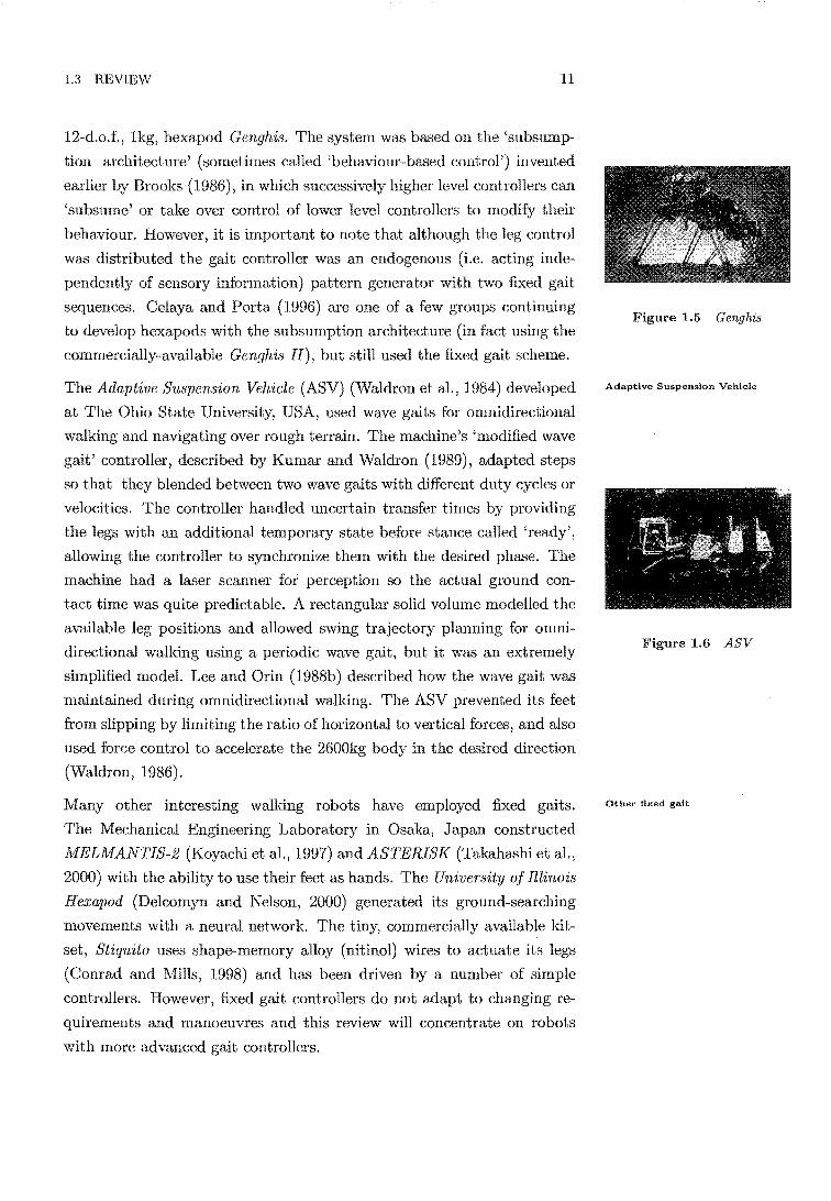
12-d.o.f., 1kg, hexapod Genghis. The system was based on the 'subsump­

tion architecture' (sometimes called 'behaviour-based control') invented

earlier by Brooks (1986), in which successively higher level controllers can

'subsume' or take over control of lower level controllers to modify their

behaviour. However, it is important to note that although the leg control

was distributed the gait controller was an endogenous (i.e. acting inde­

pendently of sensory information) pattern generator with two fIxed gait

sequences. Celaya and Porta (1996) are one of a few groups continuing

to develop hexapods with the subsumption architecture (in fact using the

commercially-available Genghis II), but still used the fIxed gait scheme.

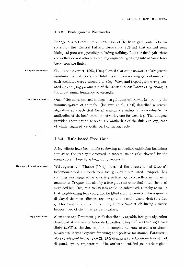
The Adaptive Suspension Vehicle (ASV) (Waldron et aI., 1984) developed

at The Ohio State University, USA, used wave gaits for omnidirectional

walking and navigating over rough terrain. The machine's 'modilied wave

gait' controller, described by Kumar and Waldron (1989), adapted steps

so that they blended between two wave gaits with different duty cycles or

velocities. The controller handled uncertain transfer times by providing

the legs with an additional temporary state before stance called 'ready',

allowing the controller to synclu'onize them with the desired phase. The

machine had a laser scanner for perception so the actual ground con­

tact time was quite predictable. A rectangular solid volume modelled the

available leg positions and allowed swing trajectory planning for omni­

directional walking using a periodic wave gait, but it was an extremely

simplifIed modeL Lee and Orin (1988b) described how the wave gait was

maintained during omnidirectional walking. The ASV prevented its feet

from slipping by limiting the ratio of horizontal to vertical forces, and also

used force control to accelerate the 2600kg body in the desired direction

(Waldron, 1986).

Many other interesting walking robots have employed fixed gaits.

The Mechanical Engineering Laboratory in Osaka, Japan constructed

MELMANTIS-2 (Koyachi et al., 1997) and ASTERISK (Takahashi et al.,

2000) with the ability to use their feet as hands. The University of Illinois

Hexapod (Deicomyn and Nelson, 2000) generated ground-searching

movements with a neural network. The tiny, commercially available kit­

set, Stiquito uses shape-memory alloy (nitinol) wires to actuate its legs

(Conrad and Mills, 1998) and has been driven by a number of simple

controllers. However, fixed gait controllers do not adapt to changing re­

quirements and manoeuvre:, and this review will concentrate on robots

with more advanced gait controllers.

Figure 1.5 Genghis

Adaptive Suspension Venic1e

Figure 1.6 ASV

Other fixed gait

Coupled oscillators

Immune networks

Extended behaviour-based

Leg phase state

12 CHAPTER 1 INTRODUCTION

1 Endogenous Networks

Endogenous networks are an extension of the fixed gait controllers, 111-

spired by the 'Central Pattern Generators' (CPGs) that control some

biological processes, possibly including walking. Like the fixed gait, these

controllers do not alter the stepping sequence by taking into account feed­

back from the limbs.

Collins and Stewart (1993, 1994) showed that some networks of six generic

non-linear oscillators could exhibit the common walking gaits of insects, if

each oscillator were connected to a leg. Wave and tripod gaits were gener­

ated by changing parameters of the individual oscillators or by changing

the input signal frequency or strength.

One of the more unusual endogenous gait controllers was inspired by the

immune system of animals. (Ishiguro et al., 1996) described a genetic

algorithm approach that found appropriate to coordinate the

antibodies of six local immune networks, one for each leg. The antigens

provided coordination between the antibodies of the different legs, each

of which triggered a specific part of the leg cycle.

1.3.4 Rule-based Free Gait

A few efforts have been made to develop controllers exhibiting behaviour

similar to the free gait observed in insects, using rules devised by the

researchers. These have been quite successfuL

Wettergreen and Thorpe (1996) described the adaptation of Brooks's

behaviour-based approach to a free gait on a simulated hexapod. Leg

stepping was triggered by a variety of fixed controllers in the same

manner as Genghis, but also by a free gait controller that lifted the most

extended leg. Requests to lift legs could be subsumed, thereby ensuring

that neighbouring legs could not be lifted simultaneously. The approach

displayed the most efficient, regular gaits but could also switch to a free

gait for rough ground or to free a leg that became stuck during a switch

between two of the other gait controllers ..

Alexandre and Preumont (1996) described a capable free gait algorithm

developed at Universite Libre de Bruxelles. They defined the 'Leg Phase

State' (LPS) as the time required to complete the current swing or stance

movement; it was negative for swing and positive for stance. Parametric

plots of adjacent leg pairs on 2D LPS diagrams (one leg on each axis) had

diagonal, cyclic, trajectories. The authors identified geometric regions

1.3 REVIEW 13

in the LPS diagrams that were statically unstable (Le. two legs lifted at

once) or ultimately led to the unstable condition. They identified rules

that corrected the trajectories to avoid the undesirable regions, either by

changing the timing of leg lifts or footfalls or (as a last resort) by reducing

the robot's velocity. In particular the rules often preempted conflict by

lifting or extending legs earlier than would normally be the case, reducing

the reliance on slowing progress to prevent stability problems. Additional

shortening or lengthening of the front and rear legs' swings promoted a

wave gait during rotation-free translations. Tests on flat ground using the

omnidirectional ULB walking machine apparently worked well although

no results were presented. The authors did not consider any uncertainty in

the footfall time (e.g. when walking over rough ground without accurate

ground perception), but halting the robot's movement would probably

handle such situations quite well.

The free gait of the 1050kg MEGANI' (Hartikainen et al., 1992) relied on

lifting the leg that was closest to becoming unable to support the robot,

or the second such leg if the first could not be lifted without actually

tipping over (Salmi and Halme, 1996). The stability was assessed using

the stability margin or by calculating the energy required to tip the robot

over. The algorithm also assessed whether any swinging leg should be

placed on the ground early to allow another leg to lift. Swing trajectories

had the maximum possible step length inside the available workspace, but

were shrunk at low speed. Simulations showed that the algorithm provided

inferior stability to the wave gait on flat ground, but was slightly superior

on rough ground.

1.3.5 Optimal Free Gait

Another approach, the most computationally intensive, is to search

amongst possible future movement combinations for the one that will

achieve the most optimal performance. This requires terrain information,

but with it the stepping required to navigate obstacles may be antici­

pated. In practice such forward planning requires strong heuristics be­

cause the number of possible moves grows exponentially with the time

ahead. For example, Chen et al. (1999) calculated that when each foot

ha.."l just 7 x 5 = 35 possible movements and the body has only 28, there are

24.5 x 106 possibilities after one timestep and 5.53 X 10184 possibilities

after forecasting ahead for 25 timesteps.

A type of free gait was implemented on the robot Ambler constructed at

MECANT

Figure 1. 7 MECANT

Figure 1.8 Ambler

Ambler

Ordinal optimization

Graph search

14 CHAPTER 1 INTRODUCTION

Carnegie Mellon University, Pennsylvania, USA (Krotkov and Simmons,

1996). This large robot had an unusual 'circulating' architecture in which

the rear legs rotated through the body to become the front legs for the

next step. This drastically reduced the search space because only the two

rear legs needed to he consin.ered as candidates for lifting. To determine

which leg to lift, the controller assumed first one and then the other rear

leg was lifted, then calculated the maximum body movement each option

allowed while still satisfying the support and kinematic constraints. For

very tight turns the front leg on the inside circulated rather than the rear

leg. Shuffling was needed occasionally to break deadlocks. Foot trajectory

planning used a terrain model generated from a laser rangefinder to select

optimal footfalls within the available movement range.

Chen et al. (1999) described simulations of a near-optimal gait controller

based on 'ordinal optimization'. Ordinal optimization says that a large

sample of randomly-selected candidates can be mathematically guaran­

teed (with some specified confidence) to be within a given range of the

optimal solution. Hence, rather than analyse every possible combination

of leg and body movements at each discrete time interval within the plan­

ning horizon, this planner assessed a large number of randomly chosen

plans and selected the best one (most stable or fastest). Because it deter­

mined the overall near-optimal behaviour for a short time into the future,

the system planned gait adjustments before reaching obstacles in its ter­

rain map. Heuristics successfully improved the plan selection process by

increasing the probability of trying long steps.

Pal and Kar (2000) reduced the number of potential movements branching

from each motion increment by restricting the leg mode combinations that

the system analysed to the 23 observed during metachronal wave gaits.

Minimum swing and stance times further reduced the number of possible

combinations, and only one leg could change mode at a time. The optimal

plan maximized the desired motion (assuming a constant heading in this

paper, but Pal et al. (1994) considered turning using the same algorithm)

while still satisfying the stability criteria. Footfalls were at the leading

edge of the leg's workspace boundary, or near it if that was not viable.

Simulation results showed that the system anticipated obstacles, adopting

a free or modified wave gait to pass them, and converged to a tripod gait

over smooth ground.

1.3 REVIEW 15

1.3.6 Distributed Free Gait

A distributed control system, in which each leg has a large degree of au­

tonomy but cooperates with its neighbours, is generally considered the

most likely paradigm for insect locomotive control. CPG models for in­

sect walking control are still supported by some researchers (for example

Delcomyn et al., 1996) but they must concede that sensory information af­

fects locomotion and it is not clear how it can be incorporated. Chapter 2

covers the evidence for a distributed system.

The TUM Walking Machine (Pfeiffer et al., 1995, Weidemann et al., 1994)

was a 23kg walker based on stick insect morphology and neurology and

constructed at the Technical University Muiichen, Germany. Leg coordi­

nation was achieved by decentralised control, whereby each leg shifted the

AEP and PEP of its neighbours by small amounts1. The main mecha­

nisms of coordination were delaying protraction (Le. a caudal shift in the

PEP) when the anterior neighbour was not on the ground or when the

contralateral leg was not on the ground. The hip caudal-rostral position

parametrically drove the other joint angles during swing. The system

achieved a stable tripod gait for forward walking after a few cycles and

was robust in the face of disturbances.

Another biologically-based way to construct a distributed gait controller

is to use neural networks. Berns et al. (1995) trained neural networks to

control the swing movements using a hand-manipulated model robot and

trained the leg coordination using data from simulations of stick insect

coordination mechanisms. The swing controllers were successfully trans­

ferred to the real robot, Lauron. The neural networks were able to climb

stairs and ditches in a simulated structured environment2 by generalizing

their basic training. Other neural networks also learnt to navigate around

obstacles by being punished after the simulated robot collided with its

environment.

Another neural network-based gait controller was Walknet from the Uni­

versity of Bielefeld, Germany (Cruse et al., 1998). The simulation Walknet

was intended to test the theory of stick insect walking control largely devel­

oped at Bielefeld (Cruse, 1990, see Chapter 2) so it was manually designed

rather than employing a learning strategy. Neural networks controlled the

swing and stance movements as well as the gait, and a mixture of positive

and negative feedback was used for the joint control. The gait control

an explanation of terms please see §1.2.3 or Fig. 2.1. 2 A structured environment is one that has simple man-made obstacles rather than

natural ones.

TUM Walking Machine

Figure 1.9 TUM walking ma­

chine

La.uron

Figure 1.10 Laur'on III

Walknet

16 CHAPTER 1 INTRODUCTION

network implemented four of the six coordinating influences found in the

animals. Kinematic simulations showed that Walknet exhibited a range of

forward walking insect gaits at different speeds and handled amputation

quite welL It was able to negotiate obstacles but could not walk in

tight curves or sideways. The scheme was also implemented on the TUM

walking machine (Dean et aL, 1999).

MAX For small hexapod MAX at the University of Salford (UK), Barnes

(1988) combined the distributed model of Cruse et aL (1998) (including a

number of modifications and simplifications) with a central pattern gener­

ator formed from coupled oscillators. The distributed controller adjusted

the phase of the CPG if there was a conflict while the CPG gradually

took control at higher speed. Experimental results showed that the robot

Case Western robots

Figure 1.11 Robot II

Age of innovation

Increasing complexity

used a tripod gait at a wider range of

properties as the distributed system.

but had the same low speed

Quinn et al. (2001) and Beer et aL (1997) described several cockroach­

inspired robots built at Case Western Reserve University, Ohio, USA .

Their later gait controllers (from Robot II) were similar to the distributed

system in stick insects (covered extensively in Chapter 2), but generaliz­

ing the forward and rearward movement limits to two-dimensional regions

gave the robot the added capabilities of turning on the spot and sideways

walking (Espenschied et aL, 1996). Full omnidirectional walking (i.e. diag­

onal walking or turning while translating) was not reported, but the robot

had to search for good footholds when walking over obstacles or

slatted surfaces.

1.3.7 Summary

An obvious law of optimization is that constraining a solution cannot

prove a result, but the technological limitations imposed on early robot i­

cists actually inspired some remarkable solutions. Anyone could have built

the simple, cheap mechanics of Genghis, but Brooks had the cunning to

produce a system that sidestepped even such fundamental issues as the

kinematics. In this era a roboticist was successful not because they could

do maths, but because they found new and ingenious ways to simplify the

problem. The solution was not more mathematical (even if that route had

been technologically feasible), it was more creative and more insightfuL

In the late eighties and early nineties increasing computational power

ered in a new era for robotics. Complicated solutions that had been pre­

viously dismissed as mere fantasy became feasible as larger and stronger

1.3 REVIEW 17

robots carried faster processors. Laser scanners, sonar and vision systems

provided details of the environment around the robot, and the machine

was expected to autonomously pick the most optimal path across obstacle

fields. Modelling included a complete dynamic model of the robot and sim­

ulations exactly replicated experimental results (Shih et al., 1987, Pfeiffer

et al., 1990, Chen et al., 1997). Additional optimisation constraints (such

as joint torque or foot force distribution) removed the inherent redundancy

of the multiple closed kinematic paths (Waldron, 1986, Weidemann et al.,

1993, Schneider and Muller, 1999, Gardner, 1991) and improving the ac­

curacy of estimates of the environmental properties tackled the problem

of the unpredictable terrain interaction (Kaneko et al., 1988, Nagy, 1993).

Thankfully the technology to deal with these escalating complexities im­

proves at the same rate. Computational power increases exponentially:

if it cannot be done in realtime now, it probably will be by the end of

next xear. Modelling and sensing technologies continue to improve and

developments in optimisation, dynamics, non-linear systems and the kine­

matics of closed loops have kept pace with the need for them.

However, after comparing the amazing progress made with walking robots

during the mid-eighties with progress in recent years, one is left with the

conclusion that progress has slowed down. In comparison, humankind's

advances in other technologies during the sarne period accelerated ad­

vances in electronics or biology now seem to be made daily.

Perhaps the problem of walking robots has become harder because the

methodology exists to deal with the increased complexity. Engineers and

scientists are trained to view problems as dispassionately as possible, so

the 'best' scientists are those who apply the most objective treatment

and the most accurate formulation of a model or equation. Finding the

problem's solution then becomes finding the solution to the model, a pro­

cess that theoretical engineering and science is ideally suited for. Rigorous

adherence to this objective scientific methodology suppresses human intu­

ition because it is decidedly subjective. However, the early walking robots

proved the worth of educated guesses, creativity and reasoning; the slow

progress more recently suggests that the field has become entrenched in

unnecessarily complex analyses.

Technology improves

Progress slowing down

A paradox

Develop new gait controller

Experimental verlfica.tion

Background chapters

Step sequencing

18 CHAPTER 1 INTRODUCTION

1

The omnidirectional manoeuvring and rough ground capabilities set walk­

ing apart from other robot locomotion technologies. However, these ad­

vantages must be coupled with efficient straight-line motion to be used

practically. There are therefore two requirements of overriding importance

to walking robots, including hexapod robots:

1. robot must have an omnidirectional manoeuvring capability.

2. It must use efficient forward (and possibly backward) walking gaits.

The objective of this study is to develop a new solution to require­

ments for a hexapod robot, in the form of a biologically-inspired gait

controller. Biological observations suggest that both requirements can be

achieved simultaneously with the same controller, and that smooth transi­

tions between the behaviours are possible. However, while careful analysis

of animal studies provides enormous insight into potential solutions, there

is no requirement (unlike some other work) to use technologies compara­

ble to those of the animal world. To decrease the system's complexity and

because insect studies show it to be nonessential, the gait controller will

avoid non-contact perception; it will sense its environment only through

contact with it.

Realistic robot testing requires real-world performance verification. Al­

though simulation is a useful tool, for practical applications the entire sys­

tem (including imperfect sensors and actuators) must be proved to work

as expected in its intended operating environment. The natural world

where gait controllers are expected to work is a particularly demanding

one where simulation has little use. Physical testing will be required to

prove the system, and in order to achieve this a real hexapod will be

constructed.

1.5

This has five chapters plus the Introduction and Conclusion. Chap-

ter 2 reviews a variety of relevant research concerning insect locomotion,

from morphology to behaviour and with an emphasis on gait control.

Chapter 3 is an overview of small hexapod Hamlet that was built

specifically for this project.

Chapter 4 begins with an analysis of the observations on control de-

1.5 OUTLINE 19

scribed in Chapter 2 and proposes an explanation of the principles that

may underly those observations. A new concept called the leg 'restrict­

edness' provides similar, but in some ways more complete, coordinating

influences to those found in the stick insect. A new gait generating algo­

rithm is developed from this explanation, and experimental results show

attractive features such as omnidirectional walking, smooth gait transi­

tions and a tripod gait over flat ground. The chapter concludes with an

analysis linking features of the implementation with particular coordinat­

ing mechanisms from biological observations.

Chapter 5 describes a new method of generating leg movements using

a 'task coordinate system'. The chapter explains how a velocity vector

field provides leg movement commands in the swing phase that are easily

adapted during the swing to the gait controller's changing requirements.

This chapter also describes the active compliance control and body atti­

tude stabilisation used in the standing legs.

Chapter 6 examines a simplified model of the gait control scheme pre­

sented in Chapter 4 and a simulation study that determined the optimum

parameters for the experimental work. Chapter 7 has conclusions and

suggestions for future enhancements, research and experiments.

Movement planning

Modelling and conclusions

CHAPTER

Observations on Insect Locomotion

Most of this work has been inspired by research observing the behaviour

of walking insects. Such 'biological inspiration' is in itself not novel and

the information in this chapter is not new, but subsequent chapters will

be clearer if the reader is familiar with the particular observations and

behaviours that are referred to. This chapter presents a relatively concise

explanation of the relevant obser"uations and theories, starting with the

general physiology. The second section describes the movement of the legs

as individuals and also the overall body movement, while the third section

examines the leg step sequencing. The final section covers the coordinating

mechanisms thought to exist in insects and the evidence for them.

1 Insect Physiology

This section gives a species~independent background of basic insect neu­

rology and morphology for the reader not familiar with these topics. An

understanding of the availability and limitations of the sense receptors

and their organisation in insects (particularly for walking) also allows us

to theorise about how they might be used. We can also discount theories

of control that cannot be supported by the available sensory informa­

tion. The primary sources were the extensive reviews by Delcomyn et aL

(1996), Graham (1985), and The Insects: Structure and Function (Chap-

Leg plane

22 CHAPTER 2 OBSERVATIONS ON INSECT LOCOMOTION

Rostral Caudal ~---.

Anterior Posterior

Prot~orax

Head Thorax Abdomen

Figure 2.1 Major insect body parts and naming of thoracic segments. This illustra­tion shows a male indigenous NZ weta, Hemideina thoracica, in a characteristic defence and stridulatory (sound-making) posture. The body length of this animal was 61mm. After Field (1978).

man, 1998).

2.1.1 Body Parts

Insects have a hard segmented exoskeleton called the cuticle made largely

of a polysaccharide called chitin. The cuticle provides structure and pro­

tection to the internal parts. Segments are joined to each other by flexible

membranes and are grouped into the head, thorax and abdomen (Fig. 2.1).

The intersegmental flexibility varies between species and segment. One

leg pair is mounted on each of the three thoracic OV!,,>UJ.Vuuo.

mesothorax and metathorax (anterior to posterior).

2.1 Structure

prothorax,

In ants, stick insects and many insect nymphs, the major plane of leg

elevation and depression (the 'leg plane') is approximately perpendicular

to the walking surface, often called the substrate. In cockroaches and

beetles it is rotated about the body's lateral axis so that it is almost

2,1 INSECT PHYSIOLOGY

TIbia

Tarsal articulation

Tarsus

Pretarsus

23

Figure 2.2 Typical insect leg showing segments and articulations, after Chapman (1998) and Weidemann et aL (1994).

parallel with the substrate. In some insects, such as stick insects, the

anterior legs operate forward of the coxa-thorax joint (a in Fig. 2.2) and

the posterior ones point caudally, pushing the animal forwards.

Each leg has six parts (Fig. 2.2). The trochanter and femur are usually

fused together and operate as one segment. The tarsus is itself segmented

but not individually articulated, and the pretarsus may have claws or

sticky pads depending on the usual walking surface of the species. The

leg parts are articulated by simple hinges, except the coxa-thorax and the

tibia-tarsus joints which are similar to a ball and socket in some insect

families. The cuticle is thicker around the joints. Muscles typically attach

to the inside of the cuticle and move the next most distal segment.

During walking the major movements are in the joints a, f3 and 1. The

6-joint is generally considered to be fixed during walkingl. Different legs

have different coxal rotations. Some families can rotate 6 to adapt to dif­

ferent terrain or usage such as defence, walking and exploring (Weidemann

et al., 1994).

1 Although Cruse and Bartling (1995) found significant movement of the coxa during stick insect walking, Frantsevich (1997) later explained their results as an artifact of the (incorrect) assumption of perfect alignment between the coxa-trochanter joint and the femur-tibia joint. There have recently been direct observations of coxa rotation in walking animals (H. Cruse, personal communication). The joint's primary use is to fold the legs for the animal's camouflage position (Dean et al., 1999).

Leg parts

Leg movements

Neurons

Neuron response

Proprioceptors

Sensory hairs a.nd spines

24 CHAPTER 2 OBSERVATIONS ON INSECT LOCOMOTION

2 .1 Neurophysiology

Neurons are the primary component of both the peripheral and central

nervous systems in animals, for information gathering and processing re­

spectively. Neurons fire in the presence of a mechanical, chemical or elec­

trical stimulus, emitting a chemically-generated electrical signal which is

carried to other neurons or to muscles. The signal is usually a series of

pulses where the frequency indicates the signal strength. A structure that

mechanically transfers a stimulus from outside the body to a neuron can

cause it to fire, providing the animal with information about the event.

:-\Aln",r,,',r neurons are located in the periphery and have projections ('ax­

ons') to the central nervous system. Stronger stimuli often cause more

rapid firing. The frequency of the firing, rather than the amplitude, en­

codes the strength of stimulus. The response to a constant input can be

itself constant ('tonic') or decreasing ('phasic'). In this way, for example,

position or velocity can be encoded by the same sort of sensory recep­

tor. The response is seldom linear over the operating range and usually

has significant hysteresis and deadzone non-linearities. Often the aggre-

range of several individual sense organs is 'range fractionated' for

improved sensitivity, so that the neurons only over certain ranges of

inputs. The combination of sensors firing and the intensity of their firing

indicates the strength of the input.

2.1.4 Leg Sensory Organs

There are eight distinct types of mechanoreceptors, that is sensors are

mechanically activated (compared to chemoreceptors which detect chem­

icals in the manner of taste and smell). The five different types of posi­

tion and movement sensing organs are together classed as proprioceptors.

They can be either inside the cuticle or outside, and measure the length

of muscles and tendons or the proximity of one part of the leg to another.

Regions of short hairs can be found around the major joints and are very

important sensors of joint position. Dean and Wendler (1983) fixed the

coxal leg hair fields in wax and rosin on stick insects and demonstrated

dependence of the leg movements during walking. Reversal of afference

from the chordotonal organ by Graham and Bassler (1981) caused in­

creased stepping on the anterior neighbour's tarsus.

External hairs and spines detect contact with the environment and other

animals, providing much of an insect's information about the external

2.1 INSECT PHYSIOLOGY 25

environment. There can be hundreds of spines per leg and thousands of

sensory hairs. are typically sensitive to only one activation plane, or

alternatively they can distinguish which direction in the plane the contact

came from.

Spines also help with walking on some surfaces in certain species. The

spines are usually curved to point towards the end of the segment so they

catch on twigs, hair or fibres even when the tarsus does not find a foothold.

Campaniform sensilla are embedded in cuticle and detect stress along

its surface. Some are more sensitive to stress in one direction, and they are

more numerous in regions of high stress. Several groups of 10-20 are found

on the trochanter where considerable force is thought to be experienced

during walking, suggesting that the accurate sensing of these forces might

be important. Campaniform sensilla may also detect contact caused by

stress in the cuticle during a collision. Other organs, the primary function

of which is not load sensing, also appear to have some ability to sense load

(Duysens et al., 2000).

2.1.5 Other Sensory Organs

Non-senso .... y spines

Stress receptors

Most adult insects have a pair of compound eyes on the head, compris- Vision

ing 1-10,000 individual units, and may also have up to three single-lens

eyes. Many insects have the ability to discriminate between different wave-

lengths of light (usually extending into the ultraviolet range but with no

sensitivity to red light) and some use binocular vision for judging dis-

tances.

Tympanal organs are an area of thin cuticle with a resonant cavity un­

derneath and allow the insect to hear. They are located on different parts

of the body in different species, often the legs or thora,-x, and are discrim­

inatory to loudness and often frequency.

All insects possess a pair of basally-articulated antenna though in some

species they may be insignificant. They are solely sensory apparatus,

principally chemical and tactile.

2,1.6 Central Nervous System

The insect central nervous system (CNS) is distributed into several lo­

cations called ganglia, with one thoracic ganglion associated with each

leg pair. The separation of the ganglia is a distinct advantage to the

Tympanal organs

Antenna

Ganglia

Neural connections

" The leg system appears to

be designed to maintain the

body in space with a suit­

able orientation relative to

the substrate."

Graham (1985)

Negative feedback

26 CHAPTER 2 OBSERVATIONS ON INSECT LOCOMOTION

researcher carrying out connective cutting experiments (in which infor­

mation flow between ganglia is interrupted) and dissections. Connectives

join the thoracic ganglia to each other and the subesophageal and suprae­

sophageal ganglia in the head. The supraesophageal (brain) pro­

cesses information from the eyes and antenna, and determines the onset,

direction and velocity of walking (Deicomyn, 1999). Sensory neurons from

the periphery may go to multiple ganglia.

Some researchers have expended considerable effort identifying which sen­

sory inputs innervate which ganglia and what their role particularly for

the locust (Altman and Kien, 1985). Some hair chordotonalorgans

and campaniform sensilla apparently playing a direct part in controlling

walking connect to neuropiles (areas of the ganglia) from which leg motor

neurons leave. None of the leg sense organs appear to convey information

directly to the contralateral side, but some have branches to ganglia in

two or three segments. Connectives from the subesophageal ganglion have

branches to each of these apparently locomotive neuropiles, and cutting

them prevents walking. This structure may not apply to other insects,

but it is reasonable to assume that the subesophageal ganglion may at

least partially coordinate walking. The connections between ganglia and

the transfer of sensory information between segments are also important

(Graham, 1985).

2.2 Leg and Body Movement

This section describes behaviour during walking that is not directly related

to the sequencing of leg movements: the movement of the legs during

stance and swing and the control of the body attitude by the stance legs.

Table 2.1 Insects commonly used for walking experiments.

lI.'rl,':II..'<".'II..'< morosus Locust Locusta migratoria American cockroach ,.< 1"""0'1111.""" "'1m americana

2.2.1 Feedback Control

Most evidence supports the idea that negative feedback controls leg and

individual joint positions. For example, by modelling the measured force

2.2 LEG AND BODY Jv10VEMENT 27

response from disturbed standing legs, Bartling and Schmitz (2000) con­

cluded that negative velocity feedback kept leg movements entrained to a

reference signal from the gait-generating system. Bassler (1977a) showed

that the I joint was under simple servo control, and the f3 and a: joints

also have reflexes that maintain a constant joint angle (Graham, 1985).

Stance /Retraction

Epstein and Graham (1983) walked stick insects on oil and found that

the front legs made brief outward movements at footfall, whereas the

other legs made inward movements. The stick insect's front are used

more for sensing than for support (as indicated by the lack of propulsive

or supportive force that they provide, Cruse, 1976b), so this may be

a mechanism for evaluating the surface. The inward movement of the

caudal pairs might help the tarsal hooks grip the substrate. Cruse (1976b)

comprehensively measured the foot forces generated by that species and

showed that, for horizontal walking, the front leg produces a decelerating

force, the hind leg an accelerating force and the middle leg a combination

of the two resulting in little (if any) net force. Bartling and Schmitz

(2000) detected short anterior and inward forces at footfall of the hind

and middle legs, which could be a mechanism for detecting the stiffness

of the substrate, or simply because the

than in the front legs.

dynamics are more significant

Wendler (1972) showed that a stick insect's body height above the ground

is servo controlled by the hair fields on the trochanter that detect the coxa-

trochanter joint angle. The insect could not hold up its own weight when

the fields were removed, but supported four times its weight with them

intact. Cruse (1976a) matched data from stick insects walking over ob­

stacles with a model where the stance legs behave as passive springs with

non-linear stiffness and he showed that the body adopts a position deter­

mined roughly by the mean slope of the substrate. The exact relationship

is complex because the intersegmental membranes can flex up to 40° up

and down. These results agree with the two proportional control constants

for walking height determined by Cruse et al. (1993). They indicate that

the behaviour, notwithstanding the discontinuity, is essentially the same

as the active compliance used on robots (Klein et al., 1983, and others,

see §5.2.3).

Substrate detection

Height control

Smooth ground

Obstacles:; body size

Searching

Anticipation

Obstacles> body size

28 CHAPTER 2 OBSERVATIONS ON INSECT LOCOMOTION

2.2.3 Swing/Protraction

The swing or protraction phase begins at the AEP and ends at the PEP.

Generally both the horizontal and the vertical amplitude (the distance

from the height at AEP to the apex of the protraction) are relatively con­

stant (Frantsevich, 1997). Because the height at AEP is not constant on

rough ground the height of the swing apex varies. Leg velocity along the

longitudinal axis is almost zero at both ends of protraction, accelerating

rapidly after liftoff and before footfall (Epstein and Graham, 1983).

Small obstacles, up to about lo of the body size, present few problems

for an insect, occasionally interfering with foot placement and grip. For

example, the tarsi of locusts walking on smooth or mesh surfaces often

make several close footfalls before selecting a good location for the step

(Pearson and Franldin, 1984). Interestingly, this behaviour was more

common on smoother, glassy surfaces.

Obstacles up to the body size require major adjustment of protraction and

the foot position relative to the body during stance. The most obvious

behaviour is the reswing or elevator in which a leg striking an object

during protraction will lift higher and attempt to clear it. This motion

is repeated and rapid, and often accompanied by a 'backing off' from the

obstacle or a rotation ofthe coxa about 5 not seen during normal walking

(Dean and Wendler, 1982).

Ditch ,-,L",OOJeut:. and precipices, where a foothold is unexpectedly not found,

elicit relatively large, rapid, exploratory movements in locusts (Pearson

and Franklin, 1984). Whether a tarsal touch on the environment is con­

sidered an obstruction or a good foothold appears to be determined by

the proximity to the anterior neighbour, at least in stick insects (Cruse

et al., 1998): if the anterior leg is nearby the touch is more likely to be

used as a foothold.

Posterior legs do not appear to use information from anterior legs to antic­

ipate the ground height. In the experiments of Cruse and Bartling (1995)

there was no soft touchdown which would indicate anticipation, though it

may exist in larger species with higher leg inertia.

Body

To traverse larger features the animal must change its whole body orien­

tation. Stick insects have a long body, and on approaching a wall perpen­

dicularly will turn diagonally to it in order to start climbing (Graham,

2.3 GAIT PATTERNS AND SELECTION 29

1985). Pearson and Franklin (1984) found that large ditches and steps

often prompted locusts to adjust their posture to simultaneously use both

the front legs to find footholds, then step in-phase with the middle legs

over the gap/step. The posture often had to be adjusted by moving the

hind legs in and taking small steps with the middle legs to make them

symmetric. If a good site still wasn't found the animals changed direction.

In Pearson and Franklin's experiments, locusts would occasionally detect

the step or ditch visibly, either slowing down or stopping. Sometimes

forelegs would lift to clear an obstacle before striking it.

2.3 Gait Patterns Selection

2.3.1 Basic Gait Model

Because of the high speed of the leg movements, the scientific analysis

of insect locomotion only became practical with the use of slow motion

film, a technique first used by Hughes (1952) with the cockroach. Wendler

(1964) pioneered another successful technique, projecting shadows of stick

insects walking on a treadmilL These papers contributed greatly to the

hypothesis of Wilson (1966), who identified the following rules that un­

derlyour modern understanding of insect gaits:

• A wave of protractions moves rostrally.

• No leg protracts until the one behind it is in stance.

• The time between a leg reaching its and the next leg protract-

ing ('protraction lag') is relatively constant.

I) The duration and length of protraction is relatively constant.

ill Because the step length is relatively constant the frequency of step­

ping determines walking speed.

All the regular insect gaits (ones where the duty factor of each leg is

the sarne as every other leg, McGhee, 1968) can be generated with these

assumptions, shown in Fig. 2.3. At all DIJ';;iv,"LD legs protract when their

posterior neighbour's protraction has completed, resulting in a rostrally­

moving wave. As the steps get more frequent (i.e. walking speed increases)

the waves start to overlap: first the different sides overlap, and eventually

successive waves on the same side overlap so that one wave starts before

Visual detection

"Historically, interest in

insect walking reaches back

at least to the seventeenth

century (and I am sure the

ancient Greeks could not

have resisted a little spec­

ulation}."

Graham (1985)

Basic principle

30 CHAPTER 2 OBSERVATIONS ON INSECT LOCOMOTION

Figure 2.3 Different gait patterns are the result of shrinldng step period (increasing step frequency), if the protraction time (black bars) and protraction lag between ipsi­lateral neighbours (grey arrows) are relatively constant. These diagrams use a constant contralateral phase of 0.5. Leg numbering follows the system in :3.3, i.e. 2 is left rear and 0 is left front. Oval boxes represent legs on one side which lift in sequence. White highlighting shows legs that lift together or close together. a) slow crawl gait: left and right sequences temporally separated, only one leg protract­ing at any time; b) wave sequences overlap, front and rear legs lift with their diagonally opposite leg; c) tetrapod wave gait: sequences overlap further, successive sequences follow immedi­ately after completion of the previous one; d) tripod gait: successive protraction sequences begin before the end of the previous one. After Wilson (1966).

2.3 GAIT PATTERNS AND SELECTION 31

Figure 2.4 Diagonal stepping with the same duty cycle as Fig. 2.3 c). Left step in time with the opposite leg on the next rostral segment.

the previous one has finished. It is important to remember that all step

frequencies in between those shown in Fig. 2.3 are viable. The diagrams

in Fig. 2.3 depict a constant contralateral phase of 0.5, meaning that legs

on opposite sides of the same segment step completely out of phase. At

least three legs remain on the ground at all times.

Constant protraction lag and duration were confirmed in the adult stick

insect (Wendler, 1964, Graham, 1972) and locust (Delcomyn, 1981). The

step length, AEP and PEP in stick insects have not been observed to

depend on the step frequency or speed of walking, although the AEP and

PEP change markedly from step to step (Epstein and Graham, 1983).

Not all of the gait patterns shown are exhibited by every insect. In some

species or life stages, protraction parameters may vary considerably with

step frequency (i.e. walking speed). When protraction lag and duration

change with walking speed the same pattern may remain over a much

larger speed range. For example, young stick insects often walk with the

tripod gait at all speeds (Graham, 1972) and cockroaches use it for all

but the slowest speeds (Delcomyn, 1981, Pearson and nes, 1973) because

the protraction time and lag decrease with increasing speed. The protrac­

tion times may be slightly different in different segments: for example in

cockroaches middle legs protract faster than hind legs (Pearson and Iles,

1973).

Contrary to later review by Graham (1985), Wilson did not assume that

contralateral phase was always 0.5 and was aware of 'diagonal stepping',

where legs swing simultaneously with the contralateral leg on the next

rostral segment (Fig. 2.4). Diagonal stepping has contralateral phase the

same as the ipsilateral phase (Fig. 2.5.a) or one minus it (Fig. 2.5.b)

depending on which side leads and which follows. Such asymmetric pat­

terns appear in stick insects (Graham, 1972) and mantids (Roeder, 1937),

and some asymmetry is sometimes observed in cockroaches (Spirito and

Mushrush, 1979)2, and can be of either handedness. Contralateral phase

Validity

Speed .. dependant parameters

a) 0 3

4

2 5

b) 0

2

Figure 2.5 Diagonal step­

ping: a) right leading left, b) left

leading right.

Shortcomings

Tight turns

32 CHAPTER 2 OBSERVATIONS OJ\" INSECT LOCOMOTION

is considerably more variable than ipsilateral phase. 'In-phase stepping'

(contralateral phase of zero) is the modus operandi of juvenile tobacco

hawk moths (Manduca sexta) (Johnston and Levine, 1996) and sometimes

in other species when they start a walk (Pearson and Franklin, 1984).

The main shortcoming with this gait model is that it does not accommo­

date the free gait observed in insects negotiating obstacles (Pearson and

Franklin, 1984, vVettergreen and Thorpe, 1996). Free gaits do not have

a repeating pattern, and are used during walks where protractions are

frequently interrupted and normal coordination becomes impossible.

Additionally, in the locust and grasshopper the back legs sometimes take

much longer steps and step ~ or ~ as often. Such 'n: l' stepping is more

common at low speeds and after prolonged walks (Graham, 1978). They

are more irregular with the faster walks.

Later experiments have shed more light on the underlying mechanisms of

coordination, but Wilson's theory that the different gait patterns emerge

from one sequential system has proven to be fundamentally correct. §2.4

covers the underlying coordinating mechanisms.

2.3.2 Turning

The primary methods of turning are modifying the step length or reducing

(eventually reversing) the stepping frequency on one side. Adult stick

insects use both techniques (Graham, 1972). Temporarily altering the

step frequency on the right and left sides so that one step is lost on

inside of the turn achieves a turn of about 20°. Alternatively, the step

length on both sides can change to a turn. In insects primarily using

the tripod gait, such as 1st instar stick insects and cockroaches, propulsive

force on the inside leg is reduced and the turn is achieved in one step.

In bees, as the turn rate increases the step length changes, followed by

the step frequency on both sides, then the inside hind leg stops while the

anterior legs step laterally, and at the highest rate of turn (a turn on

the spot) the inside legs step backwards (Zolotov et al., 1975). A tripod

pattern often appears when turning on the spot. Backward stepping has

observed in stick insects (Graham, 1985), but it is not common.

2BIinded cockroaches exhibited no asymmetry so the asymmetry is probably at-tributable to visual stimuli interacting with control - however it does demonstrate that 0.5 contralateral phase is not inviolable.

2.4 COORDINATING MECHANISMS 33

2.3.3 Starting and Stopping

Insects usually stop when all legs are on the ground, although scorpions

(Bowerman, 1981) and arachnids (Land, 1972) sometimes stop with legs

in the air and may even reverse direction halfway through a step. Some

time after stick insects stop they may move the legs into a symmetri­

cal arrangement which later necessitates several steps to regain normal

walking coordination (Dean and Wendler, 1984). Locusts starting a walk

often take a few steps where contralateral legs of the same segment step

in phase (Pearson and Franklin, 1984).

2 Obstacle Negotiation

A more stable, slower, gait allowing four or five legs to be in contact with

the ground at any time will usually be used on rougher ground. A

gait is used on very rough ground, and there are frequent occurrences of

contralateral legs stepping together when crossing ditches and climbing

large steps (Pearson and Franldin, 1984).

2 Coordinating Mechanisms

Wilson (1966), after developing his hypothesis outlined in the previous sec­

tion, concluded that walking could be best attributed to the interaction of

an endogenous oscillator (CPG) with reflex feedback which generally (but

not always) reinforces the CPG. Later researchers have tended to become

polarised towards one or the other extreme and the debate continues.

This section examines experiments revealing the underlying coordinating

mechanisms. A complete analysis and dissertation on all the relevant ex­

periments is beyond the scope of this thesis, especially as there may be

different underlying systems in different animals, but the intention is that

some insight might be had into useful models for robotics.

An isolated insect middle leg was recently shown to perform correct walk­

ing movements by Fischer et aL (2001). This lends support to the gen­

erally assumed hierarchial model, used here, that each leg has its own

'controller' that can (but doesn't usually) operate independently of the

other legs. Under this hierarchial model, the gait controller (be it cen-

tral or peripheral) influences or sets the AEP and of the legs, which

move in stance or swing until changed again. This supports the hierarchy

described in §1.2.2.

"fAJ prevailing climate of

opinion which was eager

to generalise the concept

of central oscillators has

tended to obscure the

steadily mounting evidence

that hexapods ... coordi­

nate their leg movements

on a cycle to cycle basis

via peripheral feedback."

Graham (1985)

Hierarchy

AEP targeting

Co ... activation

Immediate adaptation

Prosthetic legs

Redundancy

34 CHAPTER 2 OBSERVATIONS ON INSECT LOCOMOTION

2.4.1 Statistical Correlation

Dean and Wendler (1983) and Cruse (1979) showed in the stick insect

that the is strongly correlated with the momentary position of the

anterior neighbour: each leg steps to a position slightly behind its anterior

neighbour. The correlation was than 1, averaging about 0.8.

'AEP targeting' phenomenon was not found in the locust by Pearson and

Franklin (1984), who attributed the difference to the usual habitat of the

animals. Stick insects walk on sticks and leaf stems with sparse footholds,

while locusts inhabit the flat leaves and branches where footholds are more

abundant.

Stopping a leg during retraction elicits a stronger force in that leg due to

the servo-like behaviour described in §2.2.1, but Cruse (1985) also mea­

sured output force of the other and found a 'co-activating' influ­

ence between some of them. Ipsilateral and contralateral legs (but not

diagonal neighbours) increased their force output significantly in sympa­

thy with obstructed legs. The strength was similar caudally and rostrally

and also left and right, but it was not present between the two hind legs.

2.4.2 Amputation and Deafferentation

The amputation or disablement of a leg has been of interest to some

roboticists (for example Inagaki and KobaYB..'lhi, 1994, Weidemann et al.,

1993) and is a useful investigation for practical robots, but it is not explic­

itly a part of this research. However, amputation experiments on insects

have revealed some useful insights into their gait control.

It has long been known that insects do not require any learning time to

adapt to the amputation of a whole leg (Hughes, 1957, Graham, 1977).

Coordination is retained (with some alterations in the temporal and spa­

tial patterns) if the leg is fully removed.

Attaching a prosthetic leg in place of the amputated leg results in nor­

mal coordination again (stick insects Wendler, 1966, Delcomyn, 1985),

demonstrating that sense organs in the coxa-thorax joint or the thorax in

some way determine whether the leg is functioning. Tarsal contact is not

necessary.

Pearson and Iles (1973), working on intact but partially deafferented cock­

roaches, showed that sensory input from the coxa was not necessary for

walking, and neither WB..'l input from the tarsus, tibia and distal part of

the (together). However, removing the coxal and more distal in-

2.4 COORDINATING MECHANISMS 35

puts simultaneously "drastically diminished the animal's ability to walk" .

These experiments were carried out on decapitated animals because they

walk more readily.

The first consequence of these experiments is that they indicate that leg

coordination uSes sensory input (the force from the foot or peg leg con­

tacting the substrate). Endogenous oscillator (CPG) or fixed gait models

cannot explain this result because they provide an open-loop (synchronous

in the terminology of McGhee, 1968) setpoint or command to the leg and

therefore cannot use information from it. Hence the experiments disprove

the strictly endogenous oscillator models. Secondly, the experiments show

that sensory information from the femur, tibia and tarsus are not required

for normal walking3 . Input from the coxa-thorax joint, probably the cam­

paniform sensilla there, is sufficient to decide that a leg can be used for

walking (Delcomyn, 1985).

Pearson and Iles (1973) removed all sensory input from the legs of cock­

roaches and showed that there was still relatively normal intersegmental

coordination of the motoneurones thought to control protraction (ie: a

lack of simultaneous firing and a tendency to fire in posterior to anterior

sequence). This implies that at least some coordination in the cockroach

is central; it is not entirely due to peripheral sensory input being directly

routed to adjacent legs. In fact axons were found that appear to convey

a suitable coordinating signal between the thoracic ganglia.

Supporting this is the observation that cockroaches attempt to use a tri­

pod gait even when the middle leg is amputated. At high speeds the

influence of peripheral sensory feedback is probably reduced, perhaps be­

cause of the relatively slow conduction speed neurons compared to the

speed of walking (upwards of 20Hz). Cockroaches tend to 'sledge' on their

abdomens when running so stability from the legs is not essential, and the

importance of good coordination lessens.

On the other hand, Pearson and Iles (1973) showed a consistent increase

in lag with afferent animals over deafferented, proving that sensory input

does playa part in modifying this central coupling. Altman and Kien

(1985) described structures conveying leg sensory information to ganglia

in adjacent segments in locusts (§2.1.6).

3Insects have redundant sensory input so it does not prove that this sensory infor­mation is not used, only that it is not necessary.

the leg cycle is a

discrete sequence of move­

ments in which each part

must be successfully com­

pleted if the next part is to

" take place.

Central contral

High speed

Peripheral con.trol

Graham (1985)

Rostral inhibition

"The I d pm onge protmc-

tion of a leg does not

preclude the pmtmction of

any other leg, including the

t · . hb " an enor nezg our.

Dean and Wendler (1982)

Spatial dependence

Campaniform sensilla

Restraint

Oiled surfaces

36 CHAPTER 2 OBSERVATIONS ON INSECT LOCOMOTION

2.4.3 Interference with Leg Movement

Dean and Wendler (1982), Foth and Bassler (1985) and others have

demonstrated a rostrally-directed inhibition preventing protraction when

the posterior neighbour is protracting. The most obvious manifestation

of this behaviour is that prolonging protraction moves the of the

anterior back, Le. the anterior protraction is delayed. Dean and

Wendler (1982) reported that the inhibition was not complete: it was still

possible for the anterior leg to begin a protraction before the posterior leg

had made its footfall.

Dean and Wendler (1983), Foth and Bassler (1985) and others conducted

experiments on animals walking on treadmills where one leg at a time

stepped onto a stationary stick. The leg remained on the stick and did not

protract until the stick was moved near the normal PEP, demonstrating

that spatial rather than temporal parameters have the most significant

effect on protraction.

In contrast with the amputation of a middle leg, fixing it to the thorax

completely disables walking (cockroaches, Pearson and nes, 1973, stick

insects, Wendler, 1966). Fixing the leg stimulates the trochanteral cam­

paniform sensilla constantly, whereas amputating the leg means it is never

stimulated. Direct stimulation of the trochanteral campaniform sensilla

inhibits protraction in stick insects Bassler (1977a) and cockroaches Pear­

son and Iles (1973), suggesting that load on the leg prevents it from lift­

ing. Femoral campaniform sensilla appear to help drive the tibia during

retraction, but have little or no effect on walking coordination Akay et al.

(2001).

Restraining a stick insect middle leg in a normal walking position but

anteriorly or posteriorly to its normal middle position does not prevent

walking, but shifts the AEP and PEP of the neighbouring legs to maintain

a normal separation between them and maintain a constant step length

(Dean and ~Wendler, 1983). The step frequency on that side increased,

but there was no effect on the contralateral side.

Experiments with animals walking on oil-coated show that the me­

chanical coupling of the through the ground is very important (Ep-

stein and Graham, 1983, Cruse and Schwarze, 1988). in the treadmill

experiments the legs do not necessarily retract at the same rate: two steps

often occur when a neighbouring leg has only taken one. This indicates

that the position or velocity control of movement is very poor and that

1: 1 stepping is not rigourously enforced.

2.4 COORDINATING MECHANISMS 37

Because the removal of mechanical coupling between adjacent segments

upset the usual spatial and phase relationships between ipsilateral legs,

Cruse and Schwarze (1988) were able to observe some of the coordinating

influences used to regain normal walking. By prolonging leg retraction

they showed that:

til when a retraction of a hind leg is prolonged the end of the step is

delayed, so the position of the leg at PEP is more important than

the time since AEP;

" PEP is reached sooner the further back the anterior neighbour is,

i.e. an anterior leg tends to excite the posterior leg to protract before

it protracts itself, to favour the posterior-anterior stepping sequence;

III after leg reaching its AEP tends to excite a protraction in its anterior

neighbour.

The second observation explains the apparent inhibition of posterior leg

protractions by their anterior neighbour observed in cockroaches by Pear­

son and Iles (1973). Such caudal inhibition of protraction, in conjunction

with the rostral inhibition, should preclude simultaneous protraction of ip­

silateral neighbours: however, simultaneous protraction has in fact been

observed in the stick insect (Dean and Wendler, 1982) and the locust

(Pearson and Franklin, 1984), and occasionally leads to falls. The ap­

parent inhibition under normal circumstances is explained as follows: if

adjacent legs were retracting so that they would soon protract together,

then the anterior leg excites the posterior one to protract first, averting si­

multaneous protraction. Over difficult terrain the caudal excitation may

fail to trigger protraction in the posterior leg, and it can subsequently

begin a protraction sometime during the protraction of the anterior leg.

Cruse (1990) identified a relatively weak influence when a stick insect leg

reaches its AEP that excites the contralateral leg on the same segment

to protract. The anterior neighbour is also excited to protract at the

same time (reaching the AEP), so diagonal stepping is observed and the

contralateral phase tends towards the ipsilateral phase or 1 minus the

ipsilateral phase. This contralateral excitation influence is active over

most of the step cycle, and acts in both directions (i.e. left on right and

right on left).

Spatial relationships

No caudal inhibition

Contralateral excitation

Shortcomings

38 CHAPTER 2 OBSERVATIONS ON INSECT LOCOMOTION

2.4.4 Summary

In summary, six mechanisms for the coordination of gait have been iden­

tified Cruse (1990):

1. leg protraction is inhibited while the posterior neighbour is protract­

ing (§2.4.3);

2. protraction is excited when the posterior neighbour starts retraction

(§2.4.3);

3. protraction is excited as the anterior neighbour moves further cau­

dally (§2.4.3);

4. the AEP is correlated with the position of

(in some species, §2.4.1);

anterior neighbour

5. protraction is excited when the contralateral neighbour starts re­

tracting (§2.4.3);

6. protraction is excited when the contralateral neighbour moves fur­

ther caudally (§2.4.3).

The contralateral effects are much weaker than the ipsilateral effects,

which explains why contralateral phase is much more variable than ip­

silateral phase.

Additional influences are also necessary, some to help the legs cooperate

but not directly affecting coordination of gait patterns:

1. as legs move further posterior they protract (§2.4.3);

2. increasing leg force output increases all ipsilateral neighbours

(§2.4.1);

3. heavily loaded legs will not lift off the ground (§2.4.3).

Many experiments with fast walking species like the cockroach do not

always agree with this model, and it is thought that endogenous oscillators

may play some role (Cruse et al., 1998). Endogenous oscillators may be

required at high speeds because neural conduction of sensory information

may be too slow.

Pearson and Iles (1973), Wendler (1966) and (Bassler, 1977b) all conclu­

sively demonstrated the importance of the load-sensing campaniform sen­

silla in the gait sequence, yet the currently accepted model (Cruse et al.)

2.4 COORDINATING MECHANISMS 39

1998) does not incorporate or explain these observations. This appears to

be a significant shortcoming in the model and its resolution should be a

fruitful area of future research for biologists and roboticists.

Of more immediate importance to robotics is that the current model does

not describe the omnidirectional maneuvering behaviour that is an im­

portant capability for walking robots. Analysing the AEP and PEP in

one dimension, along the longitudinal axis of the animal, is insufficient to

form much understanding of, or gain insight into, omnidirectional walk­

ing using a free gait. Species exhibiting omnidirectional walking do not

appear to have been studied in any great depth.

The consequence is that a robot designer requiring omnidirectional ca­

pability can find little direct inspiration from the biological studies com­

pleted so far. On the other hand, Chapter 4 will describe how one liberal

interpretation of the model can lead to just this capability.

Experimental Equipment

TheTe aTe thTee ways to develop Tesults in mbotics: mathematical anal­

ysis, simulation and expeTimentation. ExpeTimental Tesults aTe the only

tTuly Teliable indication that a technique will wOTk in pmctice, and this

is paTticulaTly true of mbots intemcting with natuml envimnments. AL­

though natuml envimnment modelling is the subject of ongoing TeseaTch

(e.g. Gmnd et al., 2001), current synthetic woTlds cannot adequately con­

vey the rich variety of mechanical pmpeTties found in the Teal woTld. This

chapteT describes the haTdwaTe that was constructed fOT the experimental

wOTk, in paTticulaT a hexapod mbot (called Hamlet), its suppoTting elec­

tmnic haTdwaTe and softwaTe, and an expeTimental envimnment.

1 Requirements

This section discusses very broadly the requirements for the experimental

hardware. Carefully considering the requirements minimized the cost and

duration of construction.

1 Autonomy

The question of autonomy is of course a central theme in any project in the

rather broad field of robotics. When describing a robot as autonomous it

"The expeTiments with a

Teal mbot enSUTe that an

essence of Teality is main­

tained and that no cTiti­

cal disabling pToblems have

b . d" een ~gnoTe .

Brooks (1989)

Behavioural Autonomy

Physical Autonomy

42 CHAPTER 3 EXPERIMENTAL EQUIPMENT

is important to consider at least perfunctorily the sophistication or, more

usually, degree of autonomy. Robot designers must assess the degree

of autonomy required according to the desired mission because increasing

the autonomy complicates and expands the design.

The measurement, as far as is possible, of autonomy falls easily into two

reasonably independent spectra, for which the terms 'behavioural' and

'physical' are used.

The degree of behavioural autonomy describes the capability of the robot

to operate without supervision or control input from either a human or an­

other supervising system. Specifying behavioural autonomy encompasses

a number of decisions, including the definition of the subset of possible

exception conditions from which the robot can recover (and what consti­

tutes a recovery), and the level of abstraction of instructions given to the

robot.

The research goals of this project generate a minimum requirement for

behavioural autonomy: the robot must decide which legs to move and

how to move them, implementing gait controller part described in

§1.2.2. Autonomy at the task controller level is not specifically required

because a human operator will always be nearby. It is unnecessary to have

the ability to navigate around obstacles (or even from point to point), to

build maps or to assess the danger of a proposed movement command.

However, additional autonomy is desirable if it facilitates development,

for example automating the sensor calibration reduces the operator time

spent doing this simple but repetitive procedure, and the ability to detect

and correct faults can prevent damage to the hardware.

Physical autonomy refers to the physical independence of the robot from

external, usually fixed, systems providing power and control through a

tether and/or radio link. Much of the engineering effort expended in

constructing mobile robots, even for research, goes into providing the

robot with the ability to carry its power source and computer. This is

especially challenging for legged robots where every additional kilogram of

computer or energy storage increases energy consumption, consequently

requiring an even larger power source.

Some of the historic fascination with onboard computers and batteries

stems from a belief that to investigate behavioural autonomy the robot

must also be physically autonomous. To some degree this is true. A robot

impeded by a tether is unlikely to be able to demonstrate behavioural au­

tonomy because it will have difficulty moving effectively. However, a robot

3.2 HARDWARE DESCRlPTION 43

does not have to be seriously hampered by its tether if the link is light

and robust and the robot operates in a suitably constructed environment

or with an operator nearby. This is the case with this research allowing a

light and flexible tether and offboard processing.

3.1 Environmental

'Walking robots are often intended to work in naturally occurring envi­

ronments and this places some stringent environmental requirements on

them. The designer must consider dust, water, temperature, mechanical

robustness and even chemical resistance. Research robots having human

maintainers nearby relax these constraints somewhat, but they can be

further simplified by using the robot only indoors in a controlled environ­

ment. When the robot is not physically autonomous this has the added

advantage that the supporting equipment does not have to be protected

"The worlds where mobile

robots will do useful work

are not constructed of ex­

act simple polyhedra... It is

a mistake to bnild a special

world where the models can

be exact."

either. Brooks (1986)

3.1.3 Miscellaneous

Some miscellaneous major requirements are described below:

• The a axis (first joint axis) should have sufficient range of motion

that the leg plane of the anterior (and posterior) legs can rotate in

front (behind) the robot to allow large steps during turn-on-the-spot

manoeuvres.

• All six legs must be identical for simplicity of design and manufac­

ture.

II If possible use the TMS320C44 DSP units already available in the

Department.

<& Use DC motors because the Department had more experience with

them than other candidate actuator technologies (e.g. hydraulic,

pneumatic, brushless motors).

• Build as many parts in house as practical, because the University

does not attach a cost to workshop time for research projects but

stringently tracks purchases.

Designed at University

Chassis &; layout

44

Tether interface

DSPs

Tether

PC Joystick

CHAPTER 3 EXPERIMENTAL EQUIPMENT

Experimental environment

User

Figure 3.1 Major hardware components of the robot Hamlet and its supporting electronics.

3.2 Hardware Description

Fig. 3.1 illustrates the major hardware components used in the experi­

mental work. Virtually all the mechanical and software, and many of the

electrical, components were designed and constructed at the University

of Canterbury by the author, staff or an honours student. Further design

details are in Appendix B.

3.2.1 Hamlet

Fig. 3.2 shows a photograph of the robot Hamlet l . The major physical

properties are listed in Table. 3.1.

Fig. 3.3 shows the locations of the six identical legs and the approximate

movements available about the 0: axis (directly out of the page) for each leg

name Hamlet was sugg('~'>ted by a friend of the author with a passion for Shakespeare. The choice of the name is not a reference to any of the characteristics of the character, nor is it an acronym.

2Nominal, height varies 3Consumption of robot only, not including external components required for opera­

tion.

3.2 HARDWARE DESCRIPTION 45

Figure 3.2 Photo of Hamlet from front left quarter. The background has been largely removed from this photo for clarity.

before the chassis interferes with its movement. The chassis is constructed

of a carbon fibre composite with aluminium fittings. Vertically the leg

attachments all lie in the same plane, with all the a axes parallel.

The legs (Fig. 3.5) are all identical, machined from aluminium and have Legs

three revolute joints each. A lOvV Maxon DC motor driving through a

1:236 reduction gearbox and rated at 6Nm of torque (continuous) drives

each joint. The first two joint axes (coxa-thorax denoted by a and coxa-

femur denoted by (3) are orthogonal, and the third (femur-tibia denoted

by 1') is parallel with the second. Three axis strain gauge force sensors

are mounted at the end of each tibia inside a protective carbon fibre boot.

The tarsus is a disc mounted on a ball joint. Torsion springs provide

Table 3.1 Major physical characteristics of Hamlet.

Overall Height2 400 mm Chassis Length 400 mm Leg Length (Outstretched) 325 mm Power Supply 18 VDC Power Consumption (Electronics)3 22 W Power Consumption (Motors, Standing)3 0-30 W

Trochantor

Spring Torque

Figure 3.4 The location and

action of the f3 joint spring.

46 CHAPTER 3 EXPERIMENTAL EQCIPMENT

Figure 3.3 a-joint locations and leg numbering for Hamlet. Grey sectors are the approximate arcs inscribed by the femora when they are parallel with the chassis plane.

up to 2.5Nm of torque at each leg to help the fJ motors lower that joint

(Fig. 3.4). The motors easily overcome the springs when lifting the leg

during swing, but the springs support the robot's weight during stance so

that the motors can provide more lifting capability.

The electronics on the robot handle data acquisition and communicate

Leg attachment

Posterior·

·couPling/·

Coxa

Anterior

Chassis

Motor

--- Bevel gears

Coupling

Tibia

Protective boot

• ~Force sensor rr~i (hidden)

k;!IIl"---~- Tarsus

Leg Plane

Figure 3.5 Major parts and features of the legs, and joint axis names. The f3 joint is not visible in this diagram because the coxa and the femur hide it.

3.3 DATAFLOW 47

via a custom 4Mbit/s serial link to two Digital Signal Processors (DSPs).

The robot also receives lSV DC power for the motors through its tether

and has onboard DC-DC convertors supplying the electronics.

3.2.2 Fixed Electronics

The robot algorithms run on two Instruments TMS320C44 DSPs

mounted on an LSI daughterboard located in a PC. The DPSs commu­

nicate with another board providing a communications interface to the

tether. A Pentium 120MHz PC with an attached Logitech joystick runs

the Microsoft Windows 95 operating system and custom-written software

allowing the user to interact with the robot.

3.2.3 Experimental Environment

An L-shaped indoor experimental table was constructed measuring 3.6m

x 2.4m. Sand and rocks up to 250mm diameter generally cover the table,

although sheets of MDF ("Customwood") can be placed over the table for

experiments on hard flat surfaces. The rocks were chosen to be similar to

the rock sizes observed on Mars4 (Rover Team, 1997, Moore and Jakosky,

19S9). Most of the long end can be raised to an angle of anywhere between

0° and 300 using an electric lift jack.

3.3 Dataflow

The flow of information for the robot Hamlet is shown in the dataflow

diagram in Fig. 3.6. PC programs written specifically for the project use

the prefix 'HAM' followed by a description of their function. The list

below describes the functions of the components unique to this project:

Leg Modules

One for each leg, sampling the force sensors and position encoders,

controlling the motors and communicating with other modules and

the tether.

original intention was to create a soil mixture with similar mechanical proper­ties (friction angle, friability etc) to Martian soil. Experiments undertaken with Cathy Knight from Geological Sciences at the University of Canterbury showed that a 2:3 mix­ture of loess from Ahuriri quarry and coarse building sand from vVinstone Aggregates quarry inland from Christchurch had very similar size distribution to Martian soil. Only the sand was eventually used.

48 CHAPTER 3 EXPERIMENTAL EQUIPMENT

Figure 3.6 Dataflow diagram of the experimental hardware.

Tether Interface

On Hamlet the Leg Modules use the tether serial protocol so only

an RS-422 twisted pair interface is necessary. At the fixed end a

PC card (IS A format) provides conversion logic between HAPPE's

parallel ports and the tether.

A DSP, acting as an interface between the Client processor and the

hardware by transforming raw data to and from SI units.

Client

A DSP running software for robot control.

5 An acronym for Hardware Abstraction and Presentation ProcEssor.

3.4 CONCLUSIONS 49

DPRAM

Dual-Port RAM whih can be accessed simultaneously by the Client

DSP and the PC software.

HAMmanager

Loads and executes DSP software.

HAMdatafind

Debugging and monitoring interface to the Client, allowing inspec­

tion and modification of variables and graphing of data streams in

realtime.

HAMmessageserver

Routes debugging and status messages to other programs.

HAMcontrol

Provjdes commands and user input (eg: from the joystick) to the

Clieilt.

HAMlogger

Logs debugging and status messages for offline and pseudo-realtime

filtering and analysis.

HAMviewer

Provides instant feedback of debugging and status messages.

Matlab

A third party mathematical and data processing package, Matlab

allows data from HAMdatafind to be analysed offline.

Further information about particular blocks is in Appendix B.

3 Conclusions

Three and a half years elapsed from the beginning of Hamlet's design to

its physical completion, and there is still much that can be improved or

enhanced.

3.4.1 Problems

The peak load on the DSPs during walking occasionally exceeds the 5ms

interval available, resulting in a dropped sample. The software detects

and recovers from this situation transparently. The two DSPs currently

Dropped samples

nsps vs. pes

"nsps aTe notorious fOT

their fast paced changes on

the maTket and vendors ...

'raTely make pTovision to

inteTface oldeT boaTds with

the newer ones."

Yang (2000)

Bevel gears

Backlash

50 CHAPTER 3 EXPERIMENTAL EQUIPMENT

work sequentially, but with some changes to. their interrupt and DMA

handling software they could work in parallel and eliminate the sample

dropping.

Since this project began the speed of standard PCs has increased remark­

ably while their price has fallen. This and the availability of hard realtime

kernels or add-ons to the standard graphical operating systems (Linux and

Microsoft Windows) has made PCs an attractive option for control ap­

plications (Yang, 2000, Dunlop et aI., 1999). Using a PC in place of two

DSPs would have simplified the software and the provision of a user inter­

face and also permitted easy scaling of processing capacity. Full-featured

operating systems also have built-in inter-process communication facilities

such as pipes, shared memory and ,,,/Suu.,,,

Although the plastic bevel gears actuating the joints were expected to

wear and introduce bacldash they very well and have not worn.

However, they have been slightly damaged when sand from the experi­

mental environment has become trapped between the teeth. They are

also difficult to fix in place properly under the loads applied to them, as

pins through them (in the case of the fixed proximal gear at the {J and

"I joints) eventually become loose as the plastic deforms. Gluing them

(in the case of the distal gear going to each coupling) to a steel shaft has

never been 100% reliable. Under high loads the gears slip and the motor

position measured by the encoders no longer matches the calibrated posi­

tion of the joint. Naturally this causes problems during walking. Brass or

gears of another metal would overcome this problem because they would

be easier to secure.

The couplings and gearboxes introduce considerable backlash, making

compliance control very difficult during contact transitions. Backlash in

the {J joint leads to foot movement of up to 20mm for exam pIe. High

ratio gearboxes (1:236) were used instead of more expensive harmonic

drives (which have no backlash) because of their much lower cost. Also

the Oldham couplings may be unnecessary.

Capabilities

Apart from the limitations outlined above, the robot and other hardware

were adequate for the large amount of experimental work required. Joint

torques were sufficient in most cases, force sensors were reasonably reli­

able (provided a recalibration was carried out every hour or so), and the

range of leg movement was suitable (although further elevation of the {J

3.4 CONCLUSIONS 51

joint would an advantage when walking over obstacles). The ability

of the HAMdatafind and HAMlogger programs to record information for

offline analysis was crucial because events happen very quickly during

experiments. The joystick and graphical user interface provided an intu­

itive and easy to use way to interact with the robot, even for untrained

operators.

A helpful facility would have been the ability to videotape experiments

and trials and then to review the tape temporally correlated with the other

captured data. This would be especially useful for any future experiments

involving obstacle navigation. HAMdatafind did not capture all the data

from the robot throughout a trial because of the time spent transferring

large amounts of data between the DSPs and the PC. The user had to

decide before the experiment6 which data was going to be relevant. Ideally

all potentially relevant data would be recorded all of the time so that it

would be always available for analysis should it be needed. This capability

would be more easily implemented if a PC were used as the actual control

processor, because if its greater memory capacity.

without having to recompile any software, see Appendix B.3.2 for details of the exact capabilities of HAMdatafind and the other PC software.

Video record

Gait Patterns and Selection

This chapter describes a hexapod gait controller that allows full omni­

directional manoeuvring. The simple controller produces forward walking

results similar to those of distributed systems based on the biological obser­

vations in Chapter 2, i. e. adopting a stable periodic gait on flat surfaces.

The periodic gaits are an emergent properly of the system and are not ex­

plicitly programmed into it. The controller also provides a free gait suitable

for omnidirectional walking and navigation over rough terrain. The un­

derlying principle is that when a leg's movement is restricted it changes

from stance to swing, bringing it to a less restricted configuration while

also contributing to locomotion. Exponentially increasing fields establish

measures of leg restriction that are easily derived from the robot's physical

and software limitations. The system is easily implemented in conven­

tional functional software, and verified with experimental results from the

robot, Hamlet. The final section compares the restrictedness with the bio­

logical systems from which it was inspired.

4.1 Introduction

4.1.1 Observations, Implementation, Principles

Mimicry of the coordinating mechanisms found in insects has without Observation

Implementation

Interpretation

54 CHAPTER 4 GAIT PATTERNS AND SELECTION

Design

Principles

Behaviour

Figure 4.1 Cutaway diagram showing how the behaviour is immediately observable and the design can be copied, but determining the principles behind both require intu­ition.

doubt advanced the field of walking robotics a great deal. Cruse et al.

(1998) and Weidemann et al. (1994) for example have shown that careful

incorporation of inter-leg influences in a hexapod robot can yield a ro­

bust forward gait that maintains stability and the desired forward move­

ment, and yet also tends toward a tripod or metachronal wave gait on flat

ground.

On the other hand, the implementation technologies of biological and

robotic systems are vastly different. Although it is possible to mimic the

distributed, concurrent, computation capabilities of simple neural systems

in modern electronic hardware it is an unconventional and complicated

process. Engineers are reductionists and think of decisions sequentially;

natural systems are systemic and operate in parallel. Mapping knowledge

of biological systems directly to an implementation written in conventional

functional software running on one or two processors is, at the very least,

decidedly complicated.

Another is necessary between observation and implementation: in­

terpretation. Humans have the reasoning ability to take observations and

to generalise, compare, adapt and extend them. Our observations of the

universe are rarely observations of the system itself, but from these obser­

vations we often reason and hypothesize about the underlying principles.

Fig. 4.1 depicts the observed behaviour and the design as shells around

the underlying principles. The observer cannot see from the outside the

underlying principles, only the behaviour and how the principles are im­

plemented. Discovery of the underlying principles requires the outer layers

to be 'peeled away', as in this cutaway diagram, but they can still only

be inferred from available data.

4.1 INTRODUCTION 55

Flight by heavier than air machines is an example of this process. Early

would-be aviators constructed flapping wings in an attempt to become

airborne, following the design and behaviour of birds. However, successful

aircraft use the underlying principles of flight (the Bernoulli effect); they

do not mimic flying animals.

The same applies to the hexapod walking problem. Initial observations

were based on finding out what insects do when they walk. Recent work

has largely discovered how the behaviour emerges from the underlying

system (c.f. Chapter 2), but we have not yet fully considered why the sys­

tem is constructed in the way that it is. Why do the influences identified

in §2.4.4 exist, and is there a principle or principles behind them? This is

the ultimate extension of biologically inspired engineering.

For many problems the solution may be implemented in several alter­

native ways developed from the same solution principles. The different

implementations mayor may not display the same observable behaviour.

This is an exciting prospect for artificial hexapod walking because the

biological implementation is not really suited for conventional computer

hardware. If the principles were known they might reveal an implemen­

tation more suitable for robotics.

The implementation described in this chapter is based on a new interpre­

tation of the principles underlying the coordinating mechanisms of insects

identified in Chapter 2. The intention is to develop a new way of control­

ling a robot, not to definitively prove the principle used, so while brief

supporting evidence is given it is neither rigourous nor complete. The

results (§4.5) and a comparison of the engineering implementation with

the biological one (§4.6.1) lend some weight to the interpretation.

4.1.2 Hierarchy

§1.2.2 describes where the proposed gait controller lies in the robot's hi­

erarchy of controllers. To summarise, the role of the gait controller is to

convert the overall robot movement into sequences of leg movements and

trajectories for them to follow.

The leg movement in swing and stance modes (as opposed to the timing

of mode changes) is an important topic in its own right and is covered in

Chapter 5. For this chapter the reader can assume that the stance legs

move in unison (but with different phase) and that the swing trajectory

ends in a footfall at a favourable location some (maybe unpredictable)

Alternative implementations

Chapter outline

Implementation hierarchy

Leg movement

Aligned with movement

Individual definitions required

Rostral inhibition

56 CHAPTER 4 GAIT PATTERNS AND SELECTION

time after the transition from stance.

4.1.3 Anterior and Posterior

The algorithm presented is intended from the outset to provide walking

motion and gait control fOf omnidirectional movements across the work

surface. It will accommodate translation in any direction, rotation about

the body centroid, or a simultaneous combination of these movements.

Movement generality leaves the potential for confusion in the use of the

terms anterior and posterior previously defined in §1.2.1. Herein, when

the robot walks forwards the anterior direction, as far as movement is

concerned, lies towards the front. During pure backwards walking the an­

terior direction coincides with the robot caudal direction. Hence anterior

means in the direction of movement.

During a pure rotation (,turn on the spot') contralateral stance legs move

in opposite directions so when the term anterior (or posterior) concerns

the direction of movement it must be defined individually for each leg.

Anterior means the direction, parallel with the longitudinal axis of the

robot, that is closest to the desired body movement direction referred to

that leg. A more formal definition is given in §5.3.3. In the case of pure

sideways translation, when the movement direction is orthogonal to the

longitudinal axis, the choice of anterior and posterior is arbitrary but in

practice it has an insignificant effect.

4.2 Interpretation of Biological Observations

This section describes the coordinating influences affecting insect walk­

ing in terms of three groups: those ensuring stability, those limiting leg

restriction, and those improving gait pattern convergence.

2.1 Stability Rules

Some behaviours and inter-leg influences are clearly designed to ensure

stability of the walking animal. Not falling over is an obvious prerequisite

for walking. If the vertical projection of the centre of mass does not lie

within a region bounded by the stance legs then the animal is not statically

stable and it is likely to fall over.

The most obvious of the stability mechanisms in insects is the inhibition

4.2 INTERPRETATION OF BIOLOGICAL OBSERVATIONS 57

a) b)

Figure 4.2 Lifting any adjacent is likely to violate the static stability condition. Centre of mass is shown as black and white circle, support region as light grey. a) lifting adjacent legs on one side, b) lifting both at rostral or caudal end.

of protraction when the posterior neighbour is protracting. Fig. 4.2 shows

how lifting neighbouring legs is very likely to unbalance the insect. The

corresponding inhibition in the other direction does not technically exist,

at least in stick insects, but another excitory effect makes it unnecessary.

The effect is very similar to having a caudally directed inhibition.

Experiments show that heavily loaded insect legs do not protract. This

is a sensible behaviour, for if a leg is heavily loaded then removing its

support would probably lead to a fall.

The underlying principle appears to be that some mechanisms prevent

legs from protracting in circumstances that might, were protraction to

proceed, endanger the robot. The implicit assumption is that at some time

in the near future a safe protraction will be possible because other legs

will increase their support. It is important to note that the protraction

inhibition observed in insects is neither a necessary nor sufficient condition

to prevent the violation of the static stability of the animal.

4.2.2 Limitation of Leg Restriction

Consider an insect or robot leg very near the caudal edge of its workspace.

If the insect or robot moves forwards then the leg must protract or it will

drag over the ground. If the robot is walking backwards, the same applies

to a leg near the rostral edge of its workspace. Observations on insects

show that the further posterior a leg is the more likely it is to swing,

and the further anterior it is the more likely it is to change to stance. In

the more general 3D case a leg approaching its workspace boundary must

protract.

The fixed workspace boundaries are not the only limitations on the free

movement of legs. The proximity of neighbouring legs also obstructs their

Load protraction inhibition

Interpretation

Proximity to workspace boundary

Proximity to other legs

Essential behaviour

Possible underlying principle

58 CHAPTER 4 GAIT PATTERNS AND SELECTION

movement so if two legs are close then one should move away. \Vhen two

stance legs are close the anterior must switch to swing so it moves

away from the posterior leg. If the posterior leg is in swing mode then it

should switch to stance so that it does not get any closer to the anterior

leg1 .

These relations in insects are so basic that they are easily forgotten.

Rather than simply artifacts of the implementation they are fundamental

behaviours that stem directly from the nature of the problem. The system

absolutely must behave like this or the legs will collide or drag.

One possible underlying principle is that legs are required to change mode

when they no longer have free movement. Their free movement can be­

come restricted because of another leg approaching or because of the prox­

imity of a workspace limit. What if a more general definition of leg restric­

tion is taken, one that also takes into account the kinematic constraints

and even static torque capabilities of the robot? This work attempts to

answer that question.

4.2.3 Gait Pattern Convergence

Other biological mechanisms of walking coordination ensure that the gait

rapidly converges to a regular pattern. For example, the excitation at

a leg's AEP of it's anterior neighbour's protraction encourages the more

efficient rostrally moving wave of protractions. The excitation of the pos­

terior neighbour's protraction a.'> a leg moves caudally also has this effect.

Both these influences are also weakly active across the body, favouring

certain contralateral phase relationships. They are probably not required

for walking, but do increase walking efficiency.

4.2.4 Basic Algorithm

The following pseudo-code fragment, executed frequently during walking,

represents an implementation of a basic gait controller using the above

principles:

foreach in Legs {

if ( Leg_Mode_Is_Stance and

Leg_Is_Restricted and

AILNeighbours_Modes_Are_Stance ) then

1§5.5 covers the switch from swing to stance.

4.2 INTERPRETATION OF BIOLOGICAL OBSERVATIONS

}

else if ( Leg_Mode_Is_Swing and

Leg_Is_On_Ground ) then

Leg_Switch_To_Stance_Mode

59

10

When a standing leg becomes 'restricted' it changes to swing mode. Re­

stricted means that its current movement cannot continue because of

workspace or other constraints. The swing movement is assumed to lead

the leg to a position where it is less restricted. When the leg touches the

ground it returns to stance mode.

The algorithm incorporates the stability rules from §4.2.1 by prevent­

ing transitions to swing mode when any neighbouring legs are already in

swing. This implements bidirectional inhibition. Inhibition in the caudal

direction is logically necessary to stabilize backwards walking if forwards

walking requires rostral inhibition, so an algorithm for omnidirectional

walking must therefore provide swing inhibition in both directions.

Unidirectional inhibition where the direction depends on the robot's mo­

tion is an alternative, but in fact it does not prevent adjacent legs from

lifting and so occasionally leads to falls in insects (§2.4.3). True bidirec­

tional inhibition should reduce the chance of falling, which would be far

more serious for a relatively large robot with high inertia than for a small

insect.

Lifting both front or both rear legs simultaneously has a high likelihood

of leading to a fall, so these two pairs are considered neighbours in terms

of the basic algorithm. This extension ensures it is impossible for any two

adjacent legs to be in swing mode.

The factors responsible for improving gait convergence are not included

in this algorithm. They likely have a significant effect on the efficiency of

walking, and may make interesting future work (see §7.3.1). Note that a

convergence-assisting influence also seems to obviate the need to inhibit

protractions when the anterior neighbour is protracting; the lack of this

influence strengthens the case for bidirectional inhibition.

The next section describes a way to measure how restricted leg movements.

are using a position-dependant quantity for which the term 'restrictedness'

has been coined. The basic algorithm is an exciting new paradigm, but

its implementation uncovers numerous difficulties. These are addressed

Explanation

Bidirectional inhibition

Convergence

Characteristics

Multiple factors

Superposition function

ax depends on mode

60 CHAPTER 4 GAIT PATTERNS AND SELECTION

in §4.4.

4.3 Restrictedness

4.3.1 Measuring Restrictedness

The gait controller introduced in the previous sub-section relies on the

concept of an artificial measure of the endogenous 'restrictedness' of each

leg, for which the symbol RX will be used. Ri is a scalar describing the

lack of freedom of the i'th leg at the current time. It is endogenous because

it does not assess environmental objects or external constraints that might

additionally restrict leg movement. The restrictedness depends only on

the mode and instantaneous position of each leg and its neighbours.

Ri = 0 indicates that the movement of the i'th leg is not restricted in any

way. Ri ;:::: 1 means that the i'th is completely restricted - for example

it has collided with another part of the robot or reached the limits of its

available joint movement. As R X 1 it indicates an increasing degree of

movement restriction.

Ri is calculated from a function combining nR'" measures of restrictedness

( Ri,k' k 1,2, ... nRx). Each Ri,k models one factor that can restrict leg

i's movement. They are often the direct result of hard constraints such

as absolute maximum joint angles, but they are not necessarily physical

limitations. particular, it may be useful to include some restrictedness

components where Ri,k -t 1 as the leg nears a singularity or badly behaved

configuration.

The requirements of such a 'superposition' function to create a leg's overall

measure of restrictedness from several components are:

2. Ri ;:::: minRik ,

A suitable superposition that meets both these requirements is simply

summing individual restrictednesses:

(4.1)

where sk,m is the k'th element of a vector selecting which of the restrict-

4.3 RESTRlCTEDNESS 61

edness components should be included. Sk,m depends on the mode of the

leg, which is either swing or stance (m E {stance, sW'ing } ). For example,

Sk,stance 1 if Ri,k is to be used in stance mode and 0 otherwise. Sk,m

allows the total restrictedness to depend on different component combi­

nations in different modes.

An alternative function for the aggregate restrictedness that also fulfils

the criteria is taking the maximum of the component restrictednesses.

Equation (4.1) wa..<; used for all experiments and modelling described in

this thesis.

very convenient way to calculate each Ri k is from a function of some , directly measurable parameter qk. If qk has an allowable range from qk,min

to qk,max, then at the range extremities Ri,k 1. Outside them Rf,k > 1.

An exponential function is well suited to this purpose. It is smooth and

non-linear, meaning that as qk approaches its limits it signals restricted­

ness with rapidly increasing urgency2. Single-sided constraints have either

qk,max = 00 or qk,min = -00.

q > qk,ma,,~qk,min

q < qk,ma,,+qk,min - 2

(4.2)

In (4.2) E determines the rate at which the restrictedness takes effect as q

approaches either qk min or qk max' This is the restrictedness component's , , transition zone, or simply 'zone'. Equation (4.3) provides a suitable choice

for which Ri,k increases from 0.1 to 1 over the transition zone ~qk'

In 0.1 E=--

~qk (4.3)

4.3.2 Parameters Determining Restrictedness

Fig. 4.3 shows an appropriate set of R X components for Hamlet. The

same set of components could be easily adapted for other hexapod robots

with three degree of freedom legs and revolute joints. The parameters are

summarized in Table. 4.1, and their exact specification for Hamlet is in

Appendix C.l. See Fig. 3.5 for joint angle definitions.

Fig. 4.3.a) shows limits placed on the femur-tibia joint angle, ,.

2A linear transition could have been used, but an exponential was chosen because it commonly occurs in natural processes.

Restrictedness functions

62 CHAPTER 4 GAIT PATTERNS AND SELECTION

a) b)

e) f)

4.3 Restrictedness measurements used on Hamlet, and approximate ranges (white R X = 0, shaded R" = I). a) R"'(,) 'f-joint limit; b) R"(,B) - ,B-joint limit; c) R"'(a) a-joint limit; d) R"'(r) outer workspace limit; e) RX(s) - avoid a-axis singularity; f) RX(a.) and R"'(p.) anterior and posterior neighbours; g) R"'(a.!.) and RX(p.f.) anterior and posterior femurs. Note that the restridedness depicted in these diagrams is limited to R" :S 1, but that in the actual implementation it continues to increase beyond one outside the allowed regions.

4.3 RESTRICTED NESS 63

Table 4.1 Summary of restrictedness parameters. The femur end may be different from the location of the knee (-y-joint) in some robots, for example Hamlet.

(13) RX(a) RX(r) RX(s.) RX{a.)

(p.) RX(a.f·) RX(p.f.)

on 'Y joint Physical and software limits on 13 joint Physical limits on a joint Workspace and static torque limits a-axis singularity Proximity of anterior neighbour's foot to own foot Proximity of posterior neighbour's foot to own foot Proximity of anterior neighbour's femur end to own femur end Proximity of posterior neighbour's femur end to own femur end

The lower limit is a physical limitation of the hardware. The upper

limit is an artificial constraint to prevent the leg going through the

singularity that occurs when the leg is straight (Le. 'Y = 0).

R X (f3) f3-joint limit

Fig. 4.3.b) shows limits placed on the coxa-femur joint angle, 13. The

top limit is physical. The lower limit is artificial and prevents the

leg going into an ill behaved configuration that the simple cartesian

kinematics algorithms used in Hamlet do not handle well (the femur

pointing straight down).

RX(a) - a-joint limit

Fig. 4.3.c) shows examples of the limits on the a joints. The available

movement varies widely from leg to leg due to the shape of the

chassis and femora, and because of different wiring routes.

RX(r) - outer workspace limit

Fig. 4.3.d) illustrates the upper limit on the foot distance projected

onto the horizontal plane. RX(r) models the edge of the workspace

and limits the static torque required from the coxa-femur joint. The

simplest way to implement RX(r) is to use a circle centred on the

a-axis. Experiments with Hamlet showed that moving the centre of

the field further away from other legs and shrinking the y-axis led

to more regular stepping. Stability was also improved significantly.

§4.6.2 describes the effect of RX(r) on walking.

RX(s) - avoid a-axis singularity

Fig. 4.3.e) shows a component that prevents the foot passing through

the singularity underneath the a-axis. The singularity causes rapid

Mode dependence

64 CHAPTER 4 GAIT PATTERNS AND SELECTION

changes in a when the foot is nearly in line with the a-axis, which

can be dangerous because (at least for Hamlet) the femur can strike

the chassis and the leg wiring can be dangerously stretched. Be­

cause the changes are very rapid near the singularity the restricted­

ness method only detects them after they occur. (a) and RX(s.)

together ensure that the foot cannot go underneath the chassis.

RX(a.) and RX(p.) - anterior and posterior neighbours

Fig. 4.3.f) shows a restrictedness component increasing with the

proximity of the feet. The input is the y distance (in the robot

coordinate system) between neighbouring feet. RX(a.) is shown in

Fig. 4.a.f). RX(p.) operates on the same legs but in the other direc-

tion. It has the same value: RX(p.) for the front is the same as

RX{a.) for the middle leg. The duplication is necessary because the

middle legs have two neighbours. RX(a.) and RX(p.) only apply if

the actually has those neighbours - front have no anterior

neighbour for example.

RX(a.f.) and RX(p.J.) - anterior and posterior

Fig. 4.a.g) is similar to 4.aJ) except that it operates on the

distance between the femur ends, not the feet. The separation of

femur ends is smaller than the inter-foot distance when '"'I> 900• It

can also be smaller than RX(a.) and RX{p.) in robots like Hamlet

where the femur extends beyond the '"'I-joint (Fig. 3.5). The input

for RX(a.f.) and RX(p.f.) is the projection of the distance between

the femur ends on the of the robot.

Contralateral legs are assumed to be sufficiently separated that they can­

not collide, so legs have no effect on restrictedness on the other side of the

robot. is discussed in §7.a.L

4.3.3 Mode Dependence

In the same way that inter-leg influences in biological systems have periods

of activity and dormancy (Cruse, 1990), not all restrictednesses are active

through the whole step cycle. At the beginning of a swing the posterior

neighbour may be quite close, but a collision cannot occur because the

posterior leg will be moving caudally while the anterior one moves rostrally

(forward walking assumed). It follows that RX(p.) and RX(p.J.) are not

active during swing. Conversely, during stance the anterior neighbour

may be quite close. However, the anterior leg should not be in danger of

4.4 IMPLEMENTATION DETAILS 65

causing a collision because it will be moving away from the other leg (if

the anterior leg is in swing) or at the same rate as the other leg (if it is

in stance). RX(a.) and RX(a.f.) are therefore not active during stance.

These conditions manifest as zeros in the component selection values Sk,m'

4.4 Implementation Details

4.4.1 Increasing Restrictedness Required

Legs switch from stance to swing when they are restricted, most commonly

because they are near the edge of their workspace. The AEP is also close

to the workspace boundary3, so clearly the leg is restricted there as well.

The basic algorithm described in §4.2.4 interprets restrictedness anywhere

in the stance as the PEP condition so the leg will return to swing mode

immediately after entering stance. Therefore it seems unlikely that the

basic algorithm will lead to any useful locomotion. The same leg will

repeatedly lift and swing forward, without allowing its neighbours to lift.

The gait controllers requires a way to distinguish between restrictedness

near the AEP and near the PEP. There are several potential solutions:

Disable transition for a certain time after AEP

Two examples show that this is a poor remedy. Firstly, if the robot

movement direction changes shortly after AEP then a nearly imme­

diate return to swing might be justified. This rule would prevent

it. Secondly, if the robot slows down or stops for longer than the

inhibition lasts and while the leg is near the AEP, the leg will still

erroneously change mode. Enhancements can be conceived to fix

these errors, but the solution is basically unsatisfactory.

Disable transition until leg passes through a fixed plane

This solution requires a plane fixed in the robot coordinate system

through which every stance movement passes. On one side of the

plane the is always closer to its AEP and on the other side

always closer to its PEP. Unfortunately this cannot be guaranteed

because the mode transition points vary drastically from step to

step. The proximity of neighbouring legs can cause one step's PEP

to be further forward than the AEP of a previous step by the same

8The AEP should be near the edge of the workspace to maximize efficiency (see §5.1.1). The swing trajectory (§5.5) determines the AEP.

PEP I AEP confusion

Works fol:' omnidirectional walking

66 CHAPTER 4 GAIT PATTERNS AND SELECTION

leg. This has been observed during experiments with the robot

Hamlet. It is impossible to find a fixed plane that bisects every

stance trajectory.

Disable transition within a certain region around the AEP

Effectively using a moveable circle or other region instead of a fixed

plane, this solution has the first drawback of the first solution: it

can prevent perfectly reasonable mode changes.

Change only if restrictedness increasing

The key difference between the PEP and the AEP is that at the

former the lack of freedom is worsening, while at the latter it is

improving. This can easily be determined by looking at successive

values of the restrictedness. If:ax > 0 the leg is approaching the

PEP; if:ax < 0 the leg is departing the AEP and should not change

to swing even if it is restricted.

The fourth solution works well in all cases of omnidirectional walking.

Although it relies on the total restrictedness decreasing monotonically

after footfall (at least until R X < Rlimit), this is not an unreasonable

assumption4 . Although some restrictedness components often increase

when the leg moves away from the AEP (particulary those with decidedly

nonlinear relationships to foot position, e.g. (3- and ,-joint angles), the

rate of increase is small compared to the rate of decrease of the other

components (e.g. RX(r.) and RX(a.)). This is a difficult assertion to prove

theoretically, but the best explanation is that the increasing components

tend to be relatively insignificant near the AEP. Practical experience with

Hamlet confirmed the validity of this. :ax is easily calculated by taking

the difference between successive discrete samples.

4The 'exp' function on Hamlet (in the file tools/rts/exp.c) is the standard Texas Instruments algorithm supplied with the C40 DSP. Experiments showed that the algo­rithm is very poor. For example, the table below shows eX according to Matlab (using 8-byte IEEE floating point arithmetic and an unknown algorithm) and according to the C40 algorithm (using a proprietary 4-byte format converted to IEEE 4-byte for display by the PC).

-2.4260190 -2.4260092

eX (actual) 8.83880057 x 10 2

8.83888719 X 10-2

eX (C40) 8.83889790 x 10 8.83888868 X 10- 2

The difference between the PC results is positive (-8.6 x 10-7) but between the C40 results it is negative (1.1 x 10-7

). Because of this fault, small decreases in restrictedness component input variables occa'!ionally lead to inc/eases in their calculated restricted­ness causing frequent spurious mode transitions. Experiments showed that using the decision boundary Ii'" > 1 X 10-5 prevented these occurrences virtually all the time and still switched to swing when required.

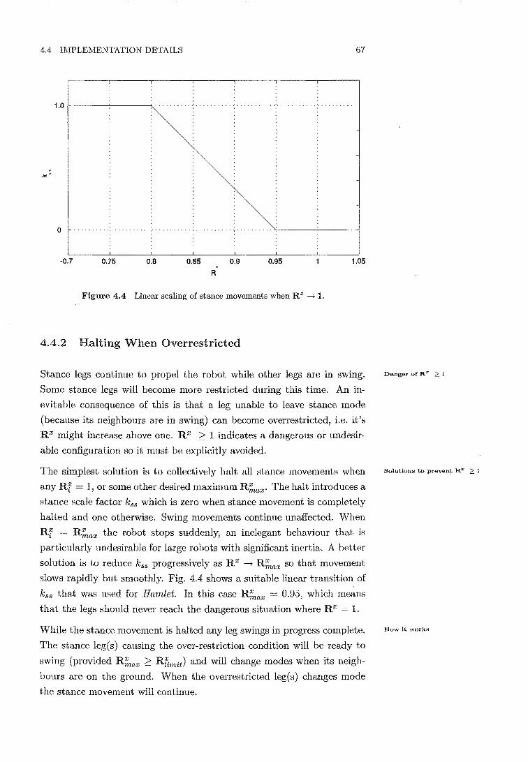
4.4 IMPLEMENTATION DETAILS 67

1.0

o .. , ........... ,,-. ------

-0.7 0.75 0.8 0.85 0.9 0.95 1.05

R

Figure 4.4 Linear scaling of stance movements when R" -t 1.

4.4.2 Halting When Overrestricted

Stance legs continue to propel the robot while other legs are in swing.

Some stance legs will become more restricted during this time. An in­

evitable consequence of this is that a leg unable to leave stance mode

(because its neighbours are in swing) can become overrestricted, i.e. it's

RX might increase above one. RX 2': 1 indicates a dangerous or undesir­

able configuration so it must be explicitly avoided.

The simplest solution is to collectively halt all stance movements when

any Rf = 1, or some other desired maximum Rihax' The halt introduces a

stance scale factor kss which is zero when stance movement is completely

halted and one otherwise. Swing movements continue unaffected. When

Rf Rihax the robot stops suddenly, an inelegant behaviour that is

particularly undesirable for large robots with significant inertia. A better

solution is to reduce kss progressively as --t Rihax so that movement

slows rapidly but smoothly. Fig. 4.4 shows a suitable linear transition of

kss that was used for Hamlet. In this case Rihax 0.95, which means

that the legs should never reach the dangerous situation where R X = 1.

While the stance movement is halted any swings in progress complete.

The stance leg(s) causing the over-restriction condition will be ready to

swing (provided Rihax 2': R Umit ) and will change modes when its neigh­

bours are on the ground. When the overrestricted leg(s) changes mode

the stance movement will continue.

Danger of R X ~ 1

Solutions to prevent Rx- :2: 1

How It works

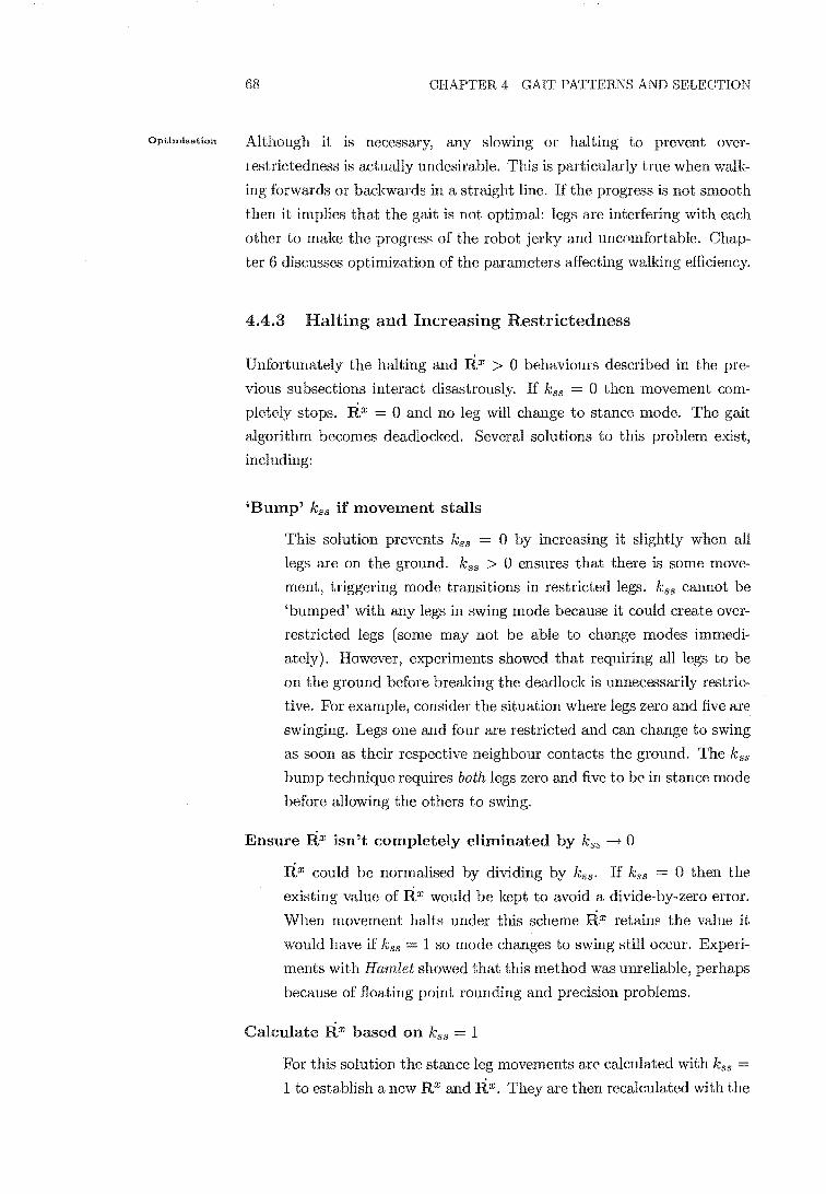
Optimisation

68 CHAPTER 4 GAlT PATTERNS AND SELECTION

Although it is necessary, any slowing or halting to prevent over­

restrictedness is actually undesirable. This is particularly true when walk­

ing forwards or backwards in a straight line. If the progress is not smooth

then it implies that the gait is not optimal: legs are interfering with each

other to make the progreSf< of the robot jerky and uncomfortable. Chap­

ter 6 discusses optimization of the parameters affecting walking efficiency.

4.4.3 Halting and Increasing Restrictedness

Unfortunately the halting and ax > 0 behaviours described in the pre­

vious subsections interact disastrously. If kss = 0 then movement com­

pletely stops. ax = 0 and no leg will change to stance mode. The gait

algorithm becomes deadlocked. Several solutions to this problem exist,

including:

'Bump' kss if movement stalls

This solution prevents kss 0 by increasing it slightly when all

legs are on the ground. kss > 0 ensures that there is some move­

ment, triggering mode transitions in restricted legs. kss cannot be

'bumped' with any legs in swing mode because it could create over­

restricted legs (some may not be able to change modes immedi­

ately). However, experiments showed that requiring all legs to be

on the ground before breaking the deadlock is unnecessarily restric­

tive. For example, consider the situation where legs zero and five are

swinging. Legs one and four are restricted and can change to swing

as soon as their respective neighbour contacts the ground. The kss

bump technique requires both legs zero and five to be in stance mode

before allowing the others to swing.

Ensure isn't completely eliminated by kss ---+ 0

ax could be normalised by dividing by kss . If kss = 0 then the

existing value of ax would be kept to avoid a divide-by-zero error.

When movement halts under this scheme ax retains the value it

would have if kss 1 so mode changes to swing still occur. Experi­

ments with Hamlet showed that this method was unreliable, perhaps

because of floating point rounding and precision problems.

Calculate ax based on kS8 = 1

For this solution the stance leg movements are calculated with kss = 1 to establish a new R X and Rx. They are then recalculated with the

4.4 IMPLEMENTATION DETAILS 69

correct kss to determine the actual restrictedness and movement, but

retaining the previously calculated Rx. This solution is then similar

to the previous one. The computational load nearly doubles.

Ignore > 0 condition when kss 0

Another solution is to ignore the RX > 0 condition when kss = O.

Vifhen movement completely stops the restrictedness no longer has

to be increasing to switch to swing. Relaxing this condition defeats

its purpose, to prevent restricted legs lifting when they are moving

to a configuration where they are less restricted. In particular legs

can be very restricted at their AEP (enough so that kss = 0) but

they should still change to swing mode only if the stance movement

makes them more restricted. Experiments showed that relaxing the

R x > 0 requirement caused spurious stepping.

Allow swing mode onset to be delayed until it is allowed

Assuming that Rfimit < R~ax (R~ax is the RX causing kss = 0)

deadlock can only occur when legs cannot lift because they have a

neighbour already in swing mode. If no neighbours were preventing

the mode transition then the leg would change to swing before be­

coming overrestricted. This observation suggests another solution:

legs 'remember' that they want to swing. Once R X > Rfimit and

> 0 they change mode at the first opportunity, i.e. when all

their neighbours are in stance mode. The transition happens even

if RX = 0 (because kss = 0) by the time the neighbours are on

the ground. If RX < 0 after latching the swing condition the mode

change is no longer necessary and is cancelled because the robot has

probably changed direction.

Experiments with Hamlet showed that the final remedy is the most

fective in almost all situations. The only case where the fifth solution is

not effective is when legs end up very restricted at their AEP due to the

swing movement (restricted enough so that kss = 0). Conservative swing

movement design (§5.5) can avoid restriction at the but adding

the first suggested solution (bumping kss ) increases reliability because it

eliminates any chance of deadlock while not overly reducing the swing.

The restricted leg (that has just made a footfall) will be at its AEP so

the 'bumped' stance movement will move it towards a lower rather than

higher RX. Other legs cannot become overrestricted because bumping

only occurs when all legs are on the ground - if they were restricted they

could change to swing mode.

Combination necessary

Leg rearl'ang~nlent

Lea.st recently used

Section outline

Using model-optimized parameters

Different gait pa.tterns

70 CHAPTER 4 GAIT PATTERNS AND SELECTION

Some insects rearrange their legs into neutral positions when they stop

walking (§2.3.3). The same behaviour can be exhibited by the robot by

artificially increasing Iix when there is no overall movement command. If

the step length is set appropriately at this time (§5.5.11) the restricted legs

rearrange to their homB positions, a more stable configuration. Also, if the

robot initializes Iix to a value greater than zero then the legs rearrange

when the gait controller is brought online. The wave gait experimental

results presented in §4.5.1 demonstrate this behaviour.

4.4.4 Swing Priority

When neighbouring legs are restricted only one can change to swing mode

at a time. Which one changes could be determined using a fixed priority,

prioritising the most restricted leg, or using a 'least recently used' (LRU)

algorithm. Many other priority schemes are also possible and the algo­

rithm choice may have an influence on walking efficiency. Hamlet uses the

LRU scheme because it promotes alternate stepping of adjacent legs. The

use of alternative priority schemes and their effect on efficiency would be

a useful future investigation.

5 Experimental Results

This section describes experiments using the robot Hamlet (Chapter 3)

that prove the restrictedness approach's capabilities. The first subsection

describes experiments demonstrating the emergence of different gaits at

different forward walking speeds and during gentle turns. The second

subsection covers manoeuvres including sideways walking, turning 'on­

the-spot', and complicated movement sequences.

All the experiments reported here were performed with the optimized

parameters determined from the model described in Chapter 6.

4.5.1 Forward Walking

Forward walking experiments showed that the restrictedness algorithm

yields the same speed-dependant gait patterns exhibited by insects (c.f.

§2.3.1). Specifically, the slow crawl, wave and tripod gaits have all been

observed at increasing walking speed, although in general the patterns do

not converge as fast as they do in insects. The results presented here are

typical of the robot's performance, not best-ca.'3e results.

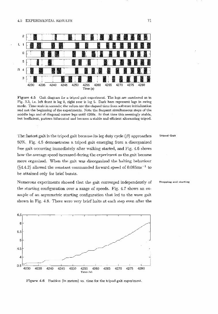
4.5 EXPERIMENTAL RESULTS

2

L

o

5

R 4

3

4230 4235 4240 4245 4250 4255 4260 4265 4270 4275 4280 Time (s)

71

Figure 4.5 Gait diagram for a tripod gait experiment. The legs are numbered as in Fig. 3.3, Le. left front is leg 0, right rear is 5. Dark bars represent legs in swing mode. Time scale in seconds; the values are the elapsed time from software initialization and not the beginning of the experiments. Note the frequent simultaneous steps of the middle and of diagonal corner legs until 4266s. At that time this seemingly stable, but inefficient, pattern bifurcated and became a stable and efficient alternating tripod.

The fastest gait is the tripod gait because its leg duty cycle ({3) approaches

50%. Fig. 4.5 demonstrates a tripod gait emerging from a disorganized

free gait occurring immediately after walking started, and Fig. 4.6 shows

how the average speed increased during the experiment as the gait became

more organized. When the gait was disorganized the halting behaviour

(§4.4.2) allowed the constant commanded forward speed of O.085ms-1 to

be attained only for brief bursts.

Numerous experiments showed that the gait converged independently of

the starting configuration over a range of speeds. Fig. 4.7 shows an ex­

ample of an asymmetric starting configuration that led to the wave gait

shown in Fig. 4.8. There were very brief halts at each step even after the

6.5.-.----,----,----,----,-----.----.----,----.----,----,---,

6

5.5

5

4.5

4

3.5 '--'----__ --L ____ -'--__ --'-____ -'-____ L-__ _

4230 4235 4240 4245 4250 4255 4260 4265 4270 4275 4280 Tim", [c:.i

4.6 Position (in metres) vs. time for the tripod gait experiment.

Tripod Gait

Stopping and starting

Turning

Omnidirectional walking

72 CHAPTER 4 GAIT PATTERNS AND SELECTION

Figure 4.7 Initial configuration for an experiment to show that the gait is robust with respect to the starting leg positions. Fig. 4.8 shows the corresponding gait pattern, a wave gait.

2

L

0

5

R 4

3

3805 3810 3815 3820 3825 3830 3835 3840 3845 3850 Time (5)

Figure 4.8 Gait diagram showing convergence to a wave pattern from the asymmetric starting configuration shown in Fig. 4.7. The results show some convergence after just one step of each leg, but the pattern did not stabilize completely until about 3845s. The commanded forward walking speed was O.04ms-1

. Note that the initial front right leg protraction occurred when the walking algorithm was initialised (before the movement command began at 3818s) to correct that leg's overrestricted state.

wave gait stabilized. Forward motion was continuous in experiments at

lower commanded speed.

'When undertaking gentle turns the inside leg stepping frequency was lower

than the outside. (At high turn rates compared to forward speed the inside

legs did not step, eventually stepping backwards when turning on the spot

- c.f. §4.5.2.) Fig. 4.9 shows the behaviour during a chicane to the right,

while Fig. 4.10 shows the different stepping frequency on the inside and

outside during the turns, particularly between 80s and 115s. The caudal­

rostral stepping sequence was lost and regained several times during the

experiment and there was little coordination between the two sides.

4.5.2 Manoeuvring

The restrictedness algorithm supports full omnidirectional walking using

£1.5 EXPERIMENTAL RESULTS 73

Figure 4.9 Sequence of photographs illustrating curve walking behaviour. 4.10 shows the gait exhibited during this experiment.

Fine control

Tul'n .. on-the-spot

74 CHAPTER 4 GAIT PATTERNS AND SELECTION

2

L

0

5

R 4

3

70 80 90 100 110 120 130 140 150 160 Time(s)

Figure 4.10 Gait diagram for curve walking experiment, walking in right then left curves of approximately 2m radius. The diagram shows a slower inside stepping fre­quency during the turns, and although the was confused the caudal-rostral sequence prevailed. The commanded forward speed was appropriate for a tripod

a free gait. Countless experiments demonstrated the ability of Hamlet to

execute turns simultaneously with sideways and! or forward movements,

using the exact same parameters as were used to achieve the regular gait

patterns described in the previous section.

The sequence of photographs in 4.11 illustrates the major interest-

ing capabilities that the restrictedness allows: sharp turns, diagonal and

sideways walking, and smooth control during the transition between dif­

ferent movement vectors. Usually the movement halted frequently during

omnidirectional movements to prevent legs becoming overrestricted, but

reducing the swing duration or commanded movement velocity allowed

smoother and more continuous omnidirectional locomotion.

Fine control (for example to avoid overshooting a target position) was

possible because the robot responded instantly5 to movement command

reductions and could accomplish very fine slow movements. Positioning

repeatability when the legs remained in contact with the ground was less

than a millimetre, but backlash and joint elasticity reduced it to around

10mm when external forces were applied to the chassis. Stepping intro­

duced large uncertainties into the dead-reckoned position even when walk­

ing on a fiat surface with good traction,for example carpet. The robot

also demonstrated a systematic tendency to turn left during the forward

walking experiments - this may have been an algorithmic or mechanical

problem.

Fig. 4.12 shows the gait diagram for an anticlockwise turn-on-the-spot

through 7f radians. Halting was frequent during this manoeuvre (not

5Within the limitations of an arbitrary lOOms command update cycle.

4.5 EXPERIMENTAL RESULTS 75

Figure 4.11 Sequence of photographs illustrating omnidirectional walking capability. Hamlet was driven by the operator so that the chassis centre followed the black line on the ground, but with some additional rotation commands. The photographs show Hamlet executing a gentle turn to its left (right in this picture); a diagonal movement to the right rear; sideways walking to the right; and a combination of walking and turning to the right blending slowly into forward walking (while still following the straight line trajectory) .

shown) because the gait was only moderately organized. The front and

rear legs have further to travel during the turn but on the left side they

took fewer steps than the middle leg, probably because of their much

greater a-axis movement range (c.f. Fig. 3.3). The gait was even less

organized at higher rotational speeds (higher duty factor) and exhibited

more frequent halting. Fielding and Dunlop (2001) described a tripod

gait emerging during similar turning experiments, but no tripod gait was

observed at any turning speed with the recent restrictedness parameters.

The a-axis range was expanded in the later experiments which may ex­

plain the difference, at least to some extent. the earlier experiments

the front and rear legs took at least as many steps as the middle legs,

rather than fewer, which supports this explanation. Allowing too much

a-axis range probably destroys the tripod pattern.

Slipping

Robustness to R X pa['ameters

76 CHAPTER 4 GAIT PATTERNS AND SELECTION

2

L

o

5

R 4

3

1050 1060 1070 1080 1090 1100 1110 1120 Time (s)

Figure 4.12 Gait diagram for anti-clockwise turn-on-the-spot through 1l" radians. The front and rear legs on the left side take fewer steps than the middle leg 011 that side.

4.5.3 Discussion

The restrictedness algorithm achieved the goals of omnidirectional walking

and implementation using conventional functional software. The scheme

proved to be reliable and effective during experiments with Hamlet. The

manoeuvring capability it affords is outstanding and the only limitation

on the movement vector that the algorithm can follow is the maximum

velocity.

Walking was extremely reliable on the carpeted surface. On the linoleum

floor and sand Hamlet had difficulty maintaining footholds and the legs

tended to slip laterally, causing major body attitude changes. The body

attitude correction (§5.2.1) corrected the deviations most of the time, but

sometimes the extra torque required exceeded the ,6-joint's capability and

the robot could not maintain its level. Large joint position errors and full

motor output showed that the problem was due entirely to the physical

limitations of the robot and not a consequence of the restrictedness al­

gorithm. Walking usually continued, although the steps were shortened

because the sunken chassis lowered the step lift height so that the legs

made footfalls soon after starting their swing. Further problems with the

hardware, specifically the need for more strength in the bonding of gears

and couplings, were noted in §3.4.1.

The modelling of the various contributors to the restrictedness was sur­

prisingly robust. The limits were easily determined from the kinematic

and static torque constraints and the design limitations of the underlying

cartesian control system. The transition zone sizes determining the rate

factors (f) were best guessed based on experience. All components were

4.6 CONCLUSIONS 77

determined before the algorithm was implemented and required virtually

no adjustment for adequate operation, although there may of course have

been an element of luck involved.

On the other hand, while walking was possible with empirically-chosen

restrictedness components it was not very efficient. The robot often be­

came stuck in apparently stable (in the sense of being able to continue

indefinitely) gaits that were extremely inefficient and required frequent

halting while leg swings were completed. Chapter 6 describes how the

components having a major effect on efficiency were optimized using a

simplified model. (r), RX(a.) and RX(p.) were the optimized compo­

nents. The walking parameters used in the results in §4.5 were selected

after this modelling.

An inefficient and distinct walking pattern was often observed where the

middle legs would step together and the diagonally opposite legs would

step together. This pattern has a maximum f3 of I so it prevents fast

walking, as seen in the tripod gait experiment in Fig. 4.5. The pattern

was marginally stable and could continue for four or more step cycles,

but eventually it always bifurcated into a more appropriate gait for the

commanded speed.

4.6 Conclusions

The key observations that support the restrictedness algorithm are that

legs change to swing mode when their movement is impeded by something,

and that the swing movement takes the to a less-restricted position.

The legs are therefore never too restricted and locomotion continues, as

long as the movements of the standing legs are properly coordinated. The

swing and stance movements are the topic of the next chapter.

The results presented in §4.5 demonstrate the two important emergent

properties of the algorithm: an omnidirectional walking capability and

convergence to the same efficient regular gaits as insects during straight

line walking. the best of the author's knowledge this combination of

desirable traits has never before been demonstrated by a artificial

gait controller, and yet the implementation of this controller is relatively

straightforward.

Efficiency

Incorrect step sequences

Inhibition

Anterior Jeg excitation

AEP targeting

Figure 4.13 Potential insta­

bility using simple inhibition

rules. Dark are on the

grOlmd, light ones are in swing.

Note that the centre of gravity

is not within the shaded support

region.

78 CHAPTER 4 GAIT PATTERNS AND SELECTION

4.6.1 Relationship to Biological Observations

It is informative to draw comparisons between the restrictedness compo­

nents (§4.3.2) and the coupling mechanisms found in insects (§2.4.4).

The simplest comparison can be made with the inhibition of swing mode

when a neighbouring is in that mode. In insects this influence is 1'OS­

trally directed only: a leg is inhibited only during its posterior neighbour's

protraction, not its anterior neighbour's. If the anterior neighbour lifts

before the leg in question (which it may do during a free gait) rostral in­

hibition does not prevent the leg from lifting. Adjacent legs then protract

simultaneously. This potentially compromises the stability when using a

free gait. The robot algorithm requires bi-directional inhibition because

it exhibits a gait, not just regular forward walking.

In insects the beginning of the posterior neighbour's retraction excites the

anterior leg's protraction. At that time the neighbouring are always in

close proximity because the posterior one is near its AEP and the other

is at its PEP. RX (p.) and R X (pI) model the proximity of a leg to its

posterior neighbour, and when the legs are close they incite the anterior

leg to swing. The effect is essentially the same as the biological influence

at the beginning of retraction.

The AEP targeting influence also emerges from the restrictedness concept.

The swing movement determines the AEP but is described in Chapter 5,

so the relationship is discussed in that chapter.

4.6.2 Stability

Preventing two adjacent legs from simultaneously being in swing mode

as used for the restrictedness gait controller is neither a necessary nor

sufficient condition for ensuring the static stability of a hexapod robot.

During steady state walking bi-directional inhibition serves very well to

prevent the robot falling over, but Fig. 4.13 shows how during a free gait

the robot can be unstable. In particular, this unstable configuration (or

close to it) was sometimes observed when Hamlet started walking. Tight­

ening (r) can reduce the step length and (since the algorithm prevents

adjacent legs from protracting simultaneously) guarantee stability on flat

ground, but smaller steps decrease efficiency.

The stability margin problem does not lend itself well to being solved on a

leg by leg basis because it requires global consideration of the leg positions

and body and leg weight distributions. Song and Waldron (1987) analysed

4.6 CONCLUSIONS 79

the stability margin for regular periodic gaits by machines or animals with

at least four legs, but the problem is not with the regular gait behaviour

so this work is of little application here.

Insects seem to achieve stability by inhibiting protraction when the sup­

port force exerted by the is high (§2A.3). That behaviour would be

well-suited to the relatively deliberative movements of a robot like Hamlet

and should enhance the robot's stability. The main obstacle would prob­

ably be ensuring that leg force actually reduced near the end of stance so

that the swing was allowed. Fortunately the centre of gravity often moves

away from the inhibited leg and therefore it would reduce the load on that

leg and allowing it to swing.

Inhibition by load

CHAPTER

Leg and Body Movement

The determination of gait patterns is a major obstacle to omnidirectional

walking, but it is not the only one. The subject of this chapter is the

movement of the legs in the stance and swing modes determined in the

previotts chapter. Leg movements control the body position with respect to

the grottnd as well as locomotion and the position of the anterior extreme

position. This chapter describes several interrelated algorithms contribttt­

ing to non-locomotive movement, a novel coordinate system derived from

the task controller's overall movement command, and the coordinate sys­

tem's application to the movement of standing and protracting legs.

perimental resttlts show that the behaviours provide very good sttpport for

omnidirectional walking.

5.1 Introduction

Chapter 4 dealt with the sequence of leg stepping, but until now the

actual leg movements have been assumed to miraculously appear when

needed. However, generating appropriate leg movements for omnidirec­

tional walking is not trivial. It is an especially complex problem when, as

a result of the application of the restrictedness concept, future movements

are somewhat chaotic and unpredictable.

next section of this chapter discusses non-locomotive movements. Outline

Exceptions

82 CHAPTER 5 LEG AND BODY MOVEMENT

a) 31.6

b)

Pigure 5.1 Passing through the centre of the workspace at Xi,home leads to longer steps. Lines are leg trajectories from one edge of the workspace to another, at constant angles. Numbers are the lengths in rum of the nearest line. a) step trajectories don't pass through Xi,home; b) steps pass through Xi,home - all steps are longer than the identical angle in a).

These are movements that do not propel the robot but achieve other,

underlying, requirements such as stability and terrain adaptation.

§5.3 introduces a 'task coordinate system' for each leg. The coordinate

system is used to describe stance movements in §5.4. The near-optimal

swing trajectory algorithm in §5.5 uses the new coordinate system so that

movements are always aligned with the desired direction of travel. The

swing trajectories use a vector field approach that has several advantages

over traditional trajectory planning. The vector field is normalized by cer­

tain parameters of the swing so that it displays the necessary adaptability

to changing demands of inter-leg coordination.

5.1.1 Stepping efficiency

Efficiency is always important for robots although it is rarely mentioned in

this thesis. However, the length of the step has a simple and direct bearing

on efficiency and must be considered. Longer steps are more efficient be­

cause fewer footfalls transfer energy to the ground. Fig. 5.1 illustrates that

to achieve the longest steps the feet should pass approximately through

the middle of their workspace during stance, a point labelled Xi,home for

each leg i. This result is important in later sections of this chapter.

For some stepping angles the longest possible steps may not pass through

Xi,homel for example a step along a vertical line in Fig. 5.1. However,

X i,home is assumed to be fixed for each leg and chosen so that these

5.2 NON-LOCOMOTIVE MOVEMENT 83

. exceptions occur only rarely in normal operation.

5.2 No·n-locomotive Movement

This section describes a method to maintain the desired ground separation

and attitude over rough terrain, a simple behaviour to maintain contact

with the ground and the compliant force control implemented on Hamlet.

The algorithms in this section apply to the legs in contact with the ground.

5.2.1 Body Attitude Feedback

The detection of ground contact at the end of the swing by force sensors

leads to varying AEP heights and therefore different stance heights. Ac­

tive compliance during the stance (§5.2.3) also causes the body attitude

and ground separation to drift. For example, when a robot approaches a

hill the front AEPs are higher, and in subsequent steps it will walk

blindly into the hill if the separation is not maintained through feedback.

Additionally, the projected centre of gravity moves towards the downhill

legs as it climbs and (with compliance) they flex, tilting the robot even

more than the underlying slope. When legs are too close or too far from

the walking surface reduces their useful workspace.

Interestingly some roboticists have advocated maintaining a gravity­

relative horizontal attitude when walking on slopes, (e.g. Klein et al.,

1983, Krotkov and Simmons, 1996). Others, with much smaller robots,

have used inaccurate but simple reflexes controlling the average roll and

pitch over all the legs to maintain a surface-relative attitude. For exam­

ple Celaya and Porta (1996) extended the balancing behaviours of Brooks

(1989)'s ground-breaking subsumption architecture to maintain a constant

attitude and separation. Wettergreen and Thorpe (1996) combined both

behaviours, using reflexive behaviours to maintain horizontal attitude.

The robot can maintain its attitude and separation relative to the ground

by adjusting the overall plane of its standing legs relative to the body xy­

plane. Adjusting all the standing legs for roll, pitch and vertical height

is like an addition to the 6-axis body movement command from the ta.'3k

controller (Fig. 5.2).

The desired plane of the ground with respect to the robot is parameterized

by pd = [zd m~ m~JT , where zd is the body-ground separation and m~

and m~ are the slope components. All the parameters are measured in the

Problem

"It should be assumed that

walking on abrupt terrain

is the typical situation for

a legged robot."

Celaya and Porta (1996)

Historical approaches

Figure 5.2 Movement axes

shared between task and atti­

tude feedback controllers.

Correcting stance

Calculating stance plane

Relevant foot positions

84 CHAPTER 5 LEG AND BODY MOVEMENT

axes of the robot coordinate system, Obody' Once the similarly defined

actual (current) stance plane pa is known, a correction proportional to the

error between each corresponding component ensures that they converge

asymptotically. The slope errors become feedback rotation rates about

the x and y axes:

(5.1 )

Kat is an attitude feedback gain vector chosen to achieve a desired expo­

nential convergence rate. Kat = [4 4 4] (99% convergence in Is) works

very well for Hamlet. Fig. 5.2 shows that the stance feedback movements • d • d

are the unused components of X body and 0body, i.e. the task-controller

and the stance controller are orthogonal. However, they are not added • d • d

into X body and fl body because they are not locomotive movements.

The parameters of the actual plane cannot be solved for more than

three standing legs except in the rare case of walking on a perfectly fiat

surface. Planar regression, shown in (5.2), calculates a minimisation of

squared error 'best fit' plane through the x y z coordinates of the n feet

considered (Wessel, 2001). All sums are performed from 1 to n, using data

from the stance legs. Equation (5.2) can be solved for using Gaussian

elimination (Engeln-Miillges and Uhlig, 1996, pg. 68). The minimisation

of squared error is similar to the body attitude behaviour observed in stick

insects (§2.2.2).

n

L; x L; x 2 L; yx

L;y L;xy y2

z

xz

yz

(5.2)

The obvious foot positions to use in (5.2) are those of the legs in stance

mode. choice works well under many circumstances because the

stance legs indicate at least three points on the ground. The current po­

sitions of any swing mode legs should definitely not be included because

they do not describe positions on the ground. However, if only stand­

ing legs are included then useful information about the ground height is

discarded when legs switch to swing. For example, with one leg on an

isolated rock in otherwise fiat terrain the body lifts on that side or corner.

When that leg changes to swing the best fit plane no longer includes the

5.2 NON-LOCOMOTIVE MOVEMENT 85

rock height, so the body becomes parallel with the flat surface. The pre­

viously elevated side or corner lowers towards the rock, having 'forgotten'

that it is there.

The last known PEP for each of the swing legs retains information about

the terrain that can be used in (5.2). A further complication exists thoug~:

XPEP is measured in robot body coordinates but it is a fixed point and

moves relative to the robot. Therefore XPEP must be updated to reflect

the fixed point's position in the robot coordinate system, then used in

(5.2). The update can be calculated by dead-reckoning with the robot

movement commands, or by using a spatial location device used for higher

level control.

There is no intrinsic reason why the attitude must converge to m~ = m~ = O. Some overall tilt may be useful when walking on hills or to carry

out some missions. For example, Schmucker et al. (1996) describe the

use of a six-legged robot for drilling and peg-in-hole tasks, both of which

require the control of all six degrees of freedom, even during the approach

to the task. and Orin (1988a) used a very similar technique to that

described here and found that allowing the body to attain some of the

underlying slope (but not all) improved stability. Setting pd by integrat­

ing commands from the task controller is similar to directly controlling

the robot's pitch, roll and height.

5.2.2 Maintaining Ground Contact

During walking over any surface of low stiffness the ground sinks under the

robot's weight. Most natural soft surfaces are also extremely non-linear,

so the surface does not return to the same level after reducing or removing

the weight. The sand used for Hamlet's experimental environment (§3.2.3)

is an excellent example of a substrate with this property of hysteresis.

vVhen the robot's weight shifts onto a leg it sinks further and the robot

tilts. Other may then lose contact with the ground as the body

tilts. The problem is particularly severe when localised surface properties

vary (for example rocks and sand) because the harder surfaces provide

a good fulcrum to tilt about. Loss of ground contact in a stance leg is

very dangerous. If its neighbouring legs lift then the weight will abruptly

return, destabilising the robot and applying large inertial loads to the

joints and legs.

Predicting the problem requires an accurate model of the ground be-

Last known X PEP

Changing ideal stance

Walking surface properties

Loss of ground contact

Maintaining ground contact

Ground following behaviour

Lowering rate

Non-zero threshold

Need for attitude feedback

86 CHAPTER 5 LEG AND BODY MOVEMENT

haviour and elevations, a model which has been assumed not to exist.

However, there are several responses to leg liftingl that can maintain con­

stant ground contact:

.. Lower any leg that loses contact with the ground.

• Raise the neighbours of any that loses contact with the ground.

• Tilt the entire robot to lower any leg that loses contact with the

ground.

III Use a sensor to determine which way the robot has tilted, and de-

termine an appropriate to raise or lower from that.

The first proposed solution is the simplest and its efficacy been proven over

many months of experiments with Hamlet and other robots (e.g. Celaya

and Porta, 1996). Any leg not in' contact with the ground is lowered

until it is. Note that, using the gait scheme in Chapter 4, if the leg does

not make contact with the ground the restrictedness will increase until it

changes to swing mode.

In Hamlet the rate of lowering is 30mm/s, which responds to most tilts

at least as rapidly as they develop. Unfortunately software and hardware

low-pass filters on the force measurements delay the response to ground

contact, causing 'chattering' if the lowering rate is too high. Chattering

is an undesirable, jerky, response where the leg makes repeated lowering

movements. The filters are necessary to remove sensor noise.

A rea..'3onably high contact force must be maintained for the leg to supply

useful support on soft surfaces. Low reaction forces do not adequately

compress the substrate and rapid sinking occurs when weight is trans­

ferred to that leg. For this reason the contact decision force must be

non-zero. In Hamlet the threshold is approximately l~O th of the over­

all weight, which works adequately although larger proportions could be

used. Experiments showed that adding hysteresis to the contact decision

can reduce chattering because it adds extra delay into the decision to start

or stop lowering, preferring to 'commit' to the current behaviour rather

than to rapidly switch between them. Fig. 5.3 shows the decision function

used on Hamlet.

Attitude and ground separation feedback, such as the system described

in §5.2.1, must be active so that contact maintaining behaviour does not

continually increase the walking height. The overall effect with attitude

1 Lifting can be detected by the drop in measured z-axis foot force.

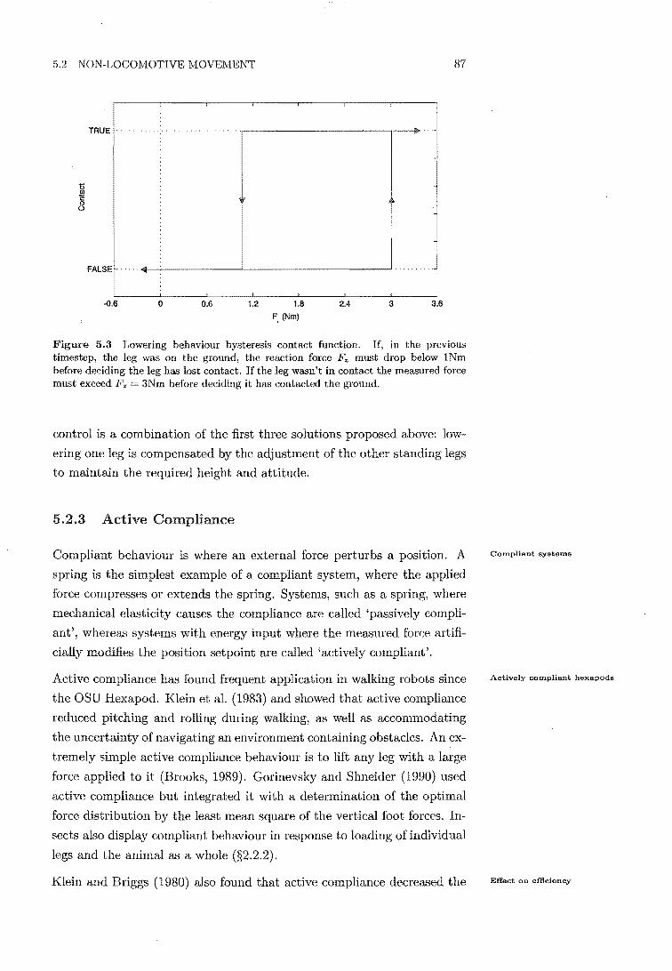
5.2 NON-LOCOMOTIVE MOVEMENT 87

TRUE

FALSE • I .....

. -0.6 0 0.6 1.2 1.8 2.4 3 3.6

F. (Nm)

Figure 5.3 Lowering behaviour hysteresis contact function. If, in the previous timestep, the leg was on the ground, the reaction force l<'z must drop below INm before deciding the leg has lost contact. If the leg wasn't in contact the measured force must exceed Fz = 3Nm before deciding it has contacted the ground.

control is a combination of the first three solutions proposed above: low­

ering one leg is compensated by the adjustment of the other standing legs

to maintain the required height and attitude.

5.2.3 Active Compliance

Compliant behaviour is where an external force perturbs a position. A

spring is the simplest example of a compliant system, where the applied

force compresses or extends the spring. Systems, such as a spring, where

mechanical elasticity causes the compliance are called 'passively compli­

ant', whereas systems with energy input where the measured force artifi­

cially modifies the position setpoint are called 'actively compliant'.

Active compliance has found frequent application in walking robots since

the OSU Hexapod. Klein et al. (1983) and showed that active compliance

reduced pitching and rolling during walking, as well as accommodating

the uncertainty of navigating an environment containing obstacles. An ex­

tremely simple active compliance behaviour is to lift any leg with a large

force applied to it (Brooks, 1989). Gorinevsky and Shneider (1990) used

active compliance but integrated it with a determination of the optimal

force distribution by the least mean square of the vertical foot forces. In­

sects also display compliant behaviour in response to loading of individual

legs and the animal as a whole (§2.2.2).

Klein and Briggs (1980) also found that active compliance decreased the

Compliant systems

Actively cotnpliant hexapods

Effect on efficiency

Foot force distribution

Active cOITlpliance equations

Stability problems

88 CHAPTER 5 LEG AND BODY MOVEMENT

antagonistic torques between legs caused by the closed kinematic chain,

thereby decreasing power consumption2 . More complex approaches to

the antagonistic torque problem rely on analysis of the whole robot, for

example the global minimization offoot interaction forces (Waldron, 1986,

Gardner, 1991) .

The co-activdtion influence between insect legs (§2.4.1) distributes propul­

sive forces evenly amongst them. The robot's kinematic control system

ensures that the stance legs move cooperatively but do not guarantee that

the foot forces will be distributed evenly, particularly on slippery or slop­

ing surfaces. Horizontal compliance evens out the foot force distribution,

effectively implementing the co-activation coordinating behaviour.

The simplest formulation of active compliance is when a Cartesian position

setpoint controls an underlying system, as is the case with Hamlet. The

measured force offsets the desired position from the higher-level controller

to create a 'commanded' position,

(5.3)

where F is the m X 1 vector of force measurements, Kac is the n x m

compliance matrix, and Xc and X d are n x 1 position vectors. nand m

can be as low as one or up to six for full force/torque control- in fact there

is no reason why m cannot exceed six, in which case there must be some

sensor redundancy. The off-diagonal elements generate cross-compliance,

i.e. a force in one axis produces a movement in another axis. This work

uses only the diagonal elements, with n = 3. The elements of Kac are

the inverses of the stiffness of each axis measured in miN (or rad/Nm for

rotational axes). Xc drives the underlying control system instead of Xd.

Assuming that the position control system is good (Le. that it is stiff and

has a rapid response), the whole system has the compliance characteristics

specified in Kac. Changing at any time changes the compliance.

Achieving stability with force control systems is notoriously difficult. Ac­

tive compliance is a class of force control and suffers the same problems,

namely sensor noise and non-linear behaviour during contact. The con­

tact non-linearity is that the surface has some finite (often extremely high)

stiffness when a manipulator (or leg) pushes against it, but zero stiffness

when it pulls away. Stability problems usually manifest themselves in

olent limit cycles where the robot repeatedly strikes the surface. The low

2The authors note that their actuators were not back-drivable so the result cannot conclusively be applied to the back-drivable servomotors on Hamlet.

5.2 NON-LOCOMOTIVE MOVEMENT 89

pass filtering required to remove force sensor noise reduces its sensitivity

to the high frequency surface impact, further compounding the problem.

Joint backlash and inertial dynamics introduce additional non-linearities.

In an active compliance system the stability boundaries create upper lim­

its on the elements of K ae , equivalent to lower limits on the stiffness.

One initial aim of this project was to use extremely compliant control to

improve walking on surfaces that change when the robot walks over them

- sand and fragile slopes especially. Hamlet was remarkably well made

considering the experience of those involved and financial constraints, but

problems with the mechanical construction (§3.4.1) precluded the use of

high gains in For example, backlash in the Oldham couplings and

gearboxes creates around 2° of free movement in the a-joints. Lightly

loading the joint gives an extra 1.5° of backlash. Although the bevel

gears were expected to be the greatest source of backlash the ability to

adjust their meshing and their plastic construction all but eliminated their

contribution.

Stabilising force control systems is the subject of extensive and ongoing

research. Of particular note, Kazerooni et a1. (1986) analysed the sta­

bility conditions of active compliance, Lawrence and Stoughton (1987)

advocated the use of additional passive compliance, and Seraji (1998)

introduced some non-linear and adaptive controllers to improve perfor­

mance. The application of these techniques to Hamlet was felt to be

beyond the scope of this thesis, but would make interesting and perhaps

worthwhile future work.

Adding a derivative term to (5.3) is the simplest way to improve active

compliance stability, and was used on Hamlet. A derivative term quickens

the reaction to making contact, but amplifies sensor noise. Table. C.2

shows the empirically-found parameters for maximum steady state com­

pliance while remaining stable. Fig. 5.4 shows the effect of adding a weight

to Hamlet using active compliance. Without active compliance the weight

does not move the robot.

5.2.4 Summary

The three components of non-locomotive movement described in this sec­

tion are interrelated. Active compliance and contact-maintaining be­

haviour together allow the legs to conform to any environment, but at­

titude feedback control is necessary for the robot to remain in a, stable

and useful stance. Active compliance without contact-maintaining does

Non .. Unearity on Hamlet

Stabilising active compliance

Stabilising Hamlet

Interrelatedness

90 CHAPTER 5 LEG AND BODY MOVEMENT

Figure 5.4 A demonstration of active compliance with Hamlet. This composite pho­tograph shows the natUl'al position and the effect of adding a 7.5kg weight to the front of the robot (left in this pictUl'e). Table. C.2 lists the stiffness parameters for the experiment.

Figure 5.5 Combined behavioUl' of non-locomotive movemcnts. The body attitude is parallel with the best fit through the standing legs. The middle legs have extended to maintain contact with the ground, while the other legs conform to the rock heights contact due to the active compliance.

5.3 TASK COORDINATE SYSTEM 91

Figure 5.6 Example of foot velocities relative to the ground for a body movement when the feet are fixed relative to the body: a clockwise rotation about z (out of the page) with simultaneous translation to the left. Light arrows show the contribution of the individual motions and dark arrows show the overall motion.

not always ensure that the feet reach the ground. Conversely, the latter

without the former does not help to achieve an even distribution of weight

amongst the legs. Attitude control without the other two behaviours does

not work because standing legs lose contact with the ground. The result

would be an incorrect attitude measurement and instability.

5.3 Task Coordinate System

5.3.1 Introduction

For any robot movement with a rotational component, the instantaneous

velocities of the individual feet relative to the body can be different

(Fig. 5.6). It could be said that each leg has its own local task to perform,

and that the task contributes to the overall task of moving the robot.

This section defines a 'task coordinate system' for each leg based on its

local task. The coordinate system is called 0' i where i is the leg number.

0' i decomposes the movements of each leg into a component contributing

to the overall task and those orthogonal to it. Movements in swing and

stance are more conveniently designed in 0' i and then converted to the

underlying kinematic controller level, in a cartesian coordinate system. A

prime distinguishes parameters in O'i from those measured in Obody.

Definition

92 CHAPTER 5 LEG AND BODY MOVEMENT

Y! .. / Y ,

/~.

0'. I

x

Figure 5.7 Definition of the task coordinate system 0' i.

5.3.2 Definition of Task Coordinate System

Consider the standing robot, with all legs on the ground in some arbi­

trary configuration at positions Xi. For a given body translational ve-

locity (X~OdY [± iI ijT) and rotational velocity about Obody (n~O£1Y [wx Wy wzjT), the velocity at the ith foot is given by the rigid body equa­

tion: ·d·£1 .£1

Xi = X bo£1y + nbo£1y X (5.4)

where X is the vector cross product operator. The 'd' superscript means

'desired', because these quantities are the desired movements given by

the higher-level controller, not the current movement rates. They do not

include any components of the non-locomotive movements. x1 is the

commanded body movement referred out to the foot, if the leg remains

fixed at its current position relative to the body. Fig. 5.6 shows an exag­

gerated example movement.

x1 defines the instantaneous orientation of the task coordinate system

O'i for each leg (Fig. 5.7). Axes in O'i are differentiated from axes in

Obody by a prime. Specifically, the definition is:

III the zi-axis is parallel with the z-axis;

III the yi-axis is parallel with the projection x1 on the xy-plane,

5.3 TASK COORDINATE SYSTEM 93

forming an angle ¢>i with y;

e O'i is centred on the nominal centre of the workspace X i,home) cho­

sen by the designer for each leg;

• the axes of O'i have the same scale as those of Obody.

Oli is a coordinate system for each leg that has its y~-axis parallel with a

tangent to the current movement of the body. The tangent to the body

movement is taken at the current foot position Xi, but the coordinate sys­

tem is actually centred on the middle of the workspace, X i,home' (§5.5.11

discusses the effect of using Xi,home to locate O'i')

The subscript i will now be dropped on scalar symbols in this chapter -

all symbols with a prime are implicitly linked with a particular leg.

I • d • d o i depends on X body and o,body, so it changes with body movement

commands. 0' i also changes with the foot position only if n:ody -# O.

O'i must not be affected by non-locomotive movement commands such as

the active compliance and body attitude stabilisation. If it is affected by

them, O'i can make sudden changes when the robot is not commanded to

move, thus causing spurious stepping3 . In practise this is easy to achieve.

5.3.3 Anterior and Posterior

The anterior and posterior direction for each leg (and therefore the neigh­

bours in that direction) can be defined using the angle ¢> in Fig. 5.7.

• The anterior direction is in the body rostral (forward) direction if =7!.. < A, < Jl 2 -<p- 2'

• The anterior direction is in the body caudal (rearward) direction

otherwise.

The transition from swing to stance must always be towards the leading

end of the robot for locomotion to be possible, i.e. towards the anterior

end. When the robot is walking backwards, the anterior neighbour is in

the caudal direction. Therefore the anterior extreme position (AEP) is

where the leg changes from swing to stance irrespective of the walking

direction, and vice versa for the PEP.

3The spurious stepping occurs because if 0' i changes due to small attitude adjust­ments the definition of anterior and posterior legs can change (see next section). This changes the restrictedness and potentially causes to step.

What is Of i exactly?

Constantly changing

0' ito ObodU

Case of o

Main cbaJlenges

Section outline

94 CHAPTER 5 LEG AND BODY MOVEMENT

For the case of ¢ = ±~ either ipsilateral neighbour could sensibly be

the anterior neighbour. The definition selects the leg in the robot rostral

direction in cases.

5.3.4 Converting to and froll! Task Coordinate System

(5.5) calculates the angle ¢ between Obody and O/i:

(5.5)

where ±d and iJd are the x and y components of respectively, and

arGian2 is the four quadrant arctangent function. A simple coordinate

translation and a rotation by ¢ about the z-axis finds X~:

The inverse of (5.6) can be found easily by recognising that rotz( -¢) is or­

thonormal (rotz( _¢)-l = rotz( _¢)T = rotz(¢)), with the last equivalence

following from sin ¢ = - sin( -¢) and cos ¢ = cos( -¢) . • d • d

When X body -flbody x Xi (the simplest example being when the robot

is stationary) then x1 = 0 and O'i cannot be defined. In these cases the

most sensible behaviour is that O'i persists with the same orientation as

before.

5.4 Stance Movement

5.4.1 Introduction

The task controller's movement command determines the majority the

movement of standing legs. After its foot contacts the ground at the

AEP, each leg is mechanically coupled to the other stance legs through • d • d

the ground and must move with them. X body and nbody prescribe its

motion implicitly.

This section analyses the stance movement in terms of movement in the

new task coordinate system O'io The restrictedness gait selection

rithm described in Chapter 4 determines the end of the stance.

5.4 STANCE MOVEMENT 95

Locomotion

The foot movement measured in Obody is the sum of the body movement

commanded by the task controller and the foot movement relative to the

body. The non-locomotive movements in §5.2 are in addition to XtodY

and ObOdYl not part of them:

·d·d ·d • Xi = X i,body + X body + !lbody X X i,body (5.7)

The feet are on the ground and stationary (unless they are slipping) so

= O. Solving for the foot movement in Obody:

• d • d • X i,body - (X body + !lbody X X i,body) (5.8)

(5.8) shows that feet fixed to the ground make the opposite movement to

the commanded body movement referred to the foot position, given by

(5.4). Because O'i is aligned with the referred motion, it follows that the

instantaneous movement of the stance legs is aligned with the y'-axis, but

in the -y' direction. The magnitude of the movement is '1/ = J x2 + iJ2. The x' component is zero, and i' z, so incremental stance movements

are generally in a plane parallel with the y' z'-plane.

Stance mode foot movements can now be calculated in 0' i. They can

of course be found directly using (5.8). Swing movements are described

more easily in O'i than in Obody, so the implementation might be simpler

if the two algorithms use the same coordinate system.

5.4.3 Ideal Stance Movement

Two points need to be made before describing the swing movement in

the next section. Firstly, if the foot passes through x' y' = 0 (i.e.

through the projection of Xi,home along the z'-axis to the ground) and

remembering that x' = 0, then the stance movement is along the y'z'­

plane, not just parallel with it. Secondly, if Obody i- 0 (and assuming

that Xi,body i- 0) or XtodY changes, then O'i (and with it, the y'z'-plane)

rotates, so while x' 0 for each incremental stance movement, previous

movements may not have been along the exact same y' zl-plane. Thus

x' i- 0 in general.

Stance movement in 0' i

Simple case

General case

Effect on stance

Swing phases and shape

Swing position

96 CHAPTER 5 LEG AND BODY MOVEMENT

5.5 Movement

5.5.1 Introduction

The swing movement control of a walking robot initially appem's to be

a trivial problem because the movement is not complicated by coupling

through the ground as it is during the stance, During forward (or re­

verse) walking the footfall should be near the front (or rear) edge of the

leg workspace, provided that the neighbouring legs will not obstruct the

movement. Inter-leg interference can easily be avoided using a fixed gait

pattern. The swing movement can be implemented simply by calculat­

ing a trajectory when the leg enters swing mode, or even by using one

pre-programmed trajectory.

The algorithms developed in this thesis are intended to provide walking

motion for omnidirectional movements across the work surface. Transla­

tion in any direction, rotation about the body centroid, or a simultaneous

combination of these movements must be possible. This complicates the

problem considerably, but swing trajectories intersecting the workspace

boundary can still be calculated (e.g. Lee and Orin, 1988b). However, the

gait generated by the system in Chapter 4 and the direction of movement

commanded by the task controller m'e not predictable from one moment

to the next, so the future location of the neighbouring (stance) legs cannot

be determined at the beginning of the swing. Because of this uncertainty

the swing movement controller must continuously evaluate the positions

of the neighbouring legs and their effect on the swinging leg.

The AEP (and therefore the swing) determines the subsequent stance

movement. Because the stance movement has a heavy influence on the

walking efficiency (§5.1.1) the swing trajectory is a critical contributor to

locomotion. The stance movement also changes continuously as the robot

movement direction changes, so the swing trajectory must react quickly

to increase the likelihood that the next stance movement will still pass

through

The swing mode can be divided into two phases, lift and extend (Fig. 5.8).

Lift moves from an arbitrm'y position on the ground towards the apex

of the swing, somewhere above Xi,home' Extend finds a footfall while

avoiding the leg in front. The shape should be something like an upside

down parabola.

When the pattern and direction of walking are fixed the transition

5.5 SWING MOVEMENT 97

Lift Extend

PEP AEP

Figure 5.8 Phases and general shape of the swing movement.

from lift to extend occurs at a known point. For omnidirectional walking

the PEP (denoted by X'pEP, or XPEP if measured in Obody) varies fTOm

step to step, as does the point of transition from lift to extend.

The step length also changes so that the AEP and PEP adjust step-by­

step for environmental and navigation disturbances varying the timing

between leg pTOtractions. Steps are also shortened to prevent the legs

from colliding with their anterior neighbour, the chassis or the edge of the

workspace.

Two parameters describe the overall dimensions of the swing. The foot

lifts to a constant height in O'i, called z~op, before descending to the AEP

at a distance approximately l~,step from the PEP (measured along y').

lLstep assumes an initial value of linitial,step at the PEP, but changes inde­

pendently for each leg during its swing. The task controller may change

z~op and hnitial,step to suit different walking enviTOnments, but they are

generally constant. In particular, the step height could be increased over

rough terrain or when sinking into a soft surface to reduce the likelihood

of swinging legs striking an obstacle.

The notation l~tep will now be used to mean the leg-specific term l~,step.

Although ziop is measured in 0' i, it is assumed to be the same for each

leg so it has no i SUbscript. This assumption is by no means essential.

l~tep and z~op have some biological justification. The average step length

is constant in insects, although it varies fTOm step to step to coordinate

walking. The swing apex is not actually constant but the vertical ampli­

tude is. Since the PEP height often does not vary much the swing apex

height (P EP+ step amplitude, i.e. z~op) is relatively consistent (§2.2.3).

A trajectory calculated at the beginning of the swing is not sufficient

for omnidirectionally walking: it must be updated regularly, potentially

continuously, throughout the movement and according to a number of

influencing factors. This section describes a new method for dealing with

all of these complexities. The task coordinate system described in §5.3

Variation of step length

Swing parameters

Biological equivalents

Section outline

Asymptotic controller

Vector field

98 CHAPTER 5 LEG AND BODY MOVEMENT

decomposes the problem neatly into two sub-problems which are dealt

with separately: the control of Xl position (§5.5.2) and movement in the

yl z'-plane (remaining subsections). yl z'-plane trajectories are calculated

using a vector field approach, with a normalization step that allows the

continuous modification of step length during swing.

5.5.2 Control of Xl

The result of the ideal swing trajectory is that the next stance movement

passes through the projection of X i,home on the ground, x' = y' = O.

However, even if robot movements are known for some time in the future,

the exact time that the stance phase will commence (and the position

of the AEP) cannot be determined with the sensory data that has been

assumed, i.e. an incomplete terrain model. Consequently the stance move­

ment cannot be predicted.

A reasonable simplification is that the current robot movement command

will continue at least until the middle of the next stance, in which case the

expectation is that the next stance movement will be wholly on the y' Zl_

plane4 . The AEP should also be on the y' zl-plane then, and a controller

for should drive x' smoothly and asymptotically to zero.

A proportional controller of the form i;' = - kX' (Hp (s) s! 1) can easily

achieve this asymptotic behaviour. The initial response of the simple

proportional controller is decidedly jerky, but a low pass filter (Hlpf(s) = can smooth it. total response is given by (5.9):

(5.9)

Fig. 5.9 is an example of x' convergence on the robot Hamlet. Note the

slightly underdamped response and that the convergence has not quite

been completed by the end of the swing. Perfect accuracy is unnecessary

because the convergence to x' = 0 is based on oversimplifying assumptions

anyway.

5.5.3 Control of yl z'

A velocity vector field provides a convenient way to specify swing motion

in yl and Z'. In a velocity vector field the foot velocity is a parametric

4 As mentioned in §5.3.2, the yl z'-plane rotates when o'body f 0 so the stance move­ment is not generally wholly on the same y' z'-plane. This point is discussed in §5.5.11.

5.5 SWING MOVEMENT 99

0.005 r-----y-------,----...,..-------,-----,-------,

o

-0.005

-0.01

-0.015

-x -0.02

-0.025

-0.03

-0.035

-0.04

-0.045'------'-------'-----'-------'------'------' 14 14.5 15 15.5

t (8) 16

5.9 Convergence of foot position to x" = O.

16.5 17

function of the position in the field. Integration of the velocity yields a

new position in the field and hence a new velocity, so vector fields are well

suited to discrete time control. Like a conventional trajectory, any given

starting point in a vector field yields a deterministic trajectory through

the field. The position in the vector field is the position of the foot in a'i; integrating the velocity from the field gives the next commanded position

in a'i.

A conventional trajectory has only one input (e.g. x' in yl = f(x' )). A ve­

locity vector field has as many inputs as outputs. (The input and output

space for the swing vector field is the y'z'-plane.) Unlike a conventional

trajectory, if an external influence moves the current point away from the

original trajectory the motion in the vector field is still defined. The ef­

fect of changing the step length 'on the fly' is to perturb the leg's position

relative to the beginning and end of the swing. The vector field accom­

modates the perturbation easily, whereas it is a major complication for a

conventional trajectory-based controller.

5.5.4 Field Normalization

The PEP, step length and step height affect the starting position and

size of the swing and therefore must affect the vector field controlling it.

X'p EP varies markedly from step to step, l~tep changes during walking,

and z~op adjusts as well, but the convex shape of the trajectory should

USnAHY UNIVERSITY OF CANTERBURY

CHRISTCHURCH. N.Z,

Advantages

Changing field boundaries

100 CHAPTER 5 LEG AND BODY MOVEMENT

1.2.-----.-------.----,---

0,8 z'

0.6 'N

0.4

0.2 y' = y'", + /.,.,

0

PEP AEP -0.2

-0.2 o 0,2 0.4 0.6 0,8 1.2 y'

Figure 5.10 Relationship between position in the task coordinate system 0' i and the swing-normalized position. y* and z· are the swing-normalized y' and z' positions respectively.

persist.

Normalizing the current positions before evaluating the vector field ac­

commodates these difficulties. y' and Zl positions are converted to 'swing­

normalized' positions y* and z* that are used to identify the current po­

sition in the vector field. The normalization adjusts for the different PEP

and step length of each leg, and for the step height. The swing-normalized

field the following properties:

• the PEP is at y* = z* = OJ

• the AEP is at y* = 1;

• the apex is at z* = 1.

(5.10) and (5.11) convert between the two systems. When the step length

\Ju,cw..,;GC) in mid-swing the normalized position changes. If it then

the normalized position (Fig. 5.10) illustrates the relatiOll.';.;hip between O'i

and swing-normalized coordinates.

y*

z*

y' I YPEP

l~tep I I

Z - zPEP I I

Ztop - zpEP

(5.10)

(5.11)

5.5 SWING :\10VEMENT 101

Velocities can be converted by the differentials of (5.10) and (5.11):

il i/ (5.12)

it (5.13)

Because the leg mostly moves monotonically between y'pEP and y'pEP + l~tep, y* will rarely be outside range [0, :l].

5.5.5 Field Design

Another advantage of using a vector field is that the swing can be broken

into localised or simplified micro-fields that are superimposed using addi­

tion. If the component micro-fields have 'soft' edges they blend together

smoothly so the trajectories through the total field are smooth. The com­

ponents proposed in this subsection are fields acting in a single direction

(or radiating from the centroid of the field) and with simple shapes

lipses and lines. Fig. 5.11 shows the micro-fields used for Hamlet. They

are listed in Table. 5.1.

Table 5.1 Swing movement decomposition into micro-fields. Appendix C.3 tables the exact field specifications.

Name Constant PEP Boost

t Ztop

Centre Corner AEP

Description Move leg towards AEP, active over whole y*z*-plane Lift leg when it is near Continue lifting leg on its way to the apex Prevent leg from lifting above the apex Keep leg out of the centre Start leg extending before it to the AEP Stop leg from passing AEP and extend it as it approaches

The Constant micro-field in Table. 5.1 simply points rightward - it is

not shown in Fig. 5.11. Constant is responsible for the general y*-axis

progression from PEP to AEP. The part of the swing should lift and

must cancel out Constant (which might otherwise cause the foot to drag

across the ground) so the PEP micro-field is added near the PEP. The

Boost micro-field is not as strong as PEP so that the lifting slows and the

Constant micro-field starts some forward swing. z~op prevents the foot

from going above the apex and pushes it down if it does get there (which

is possible if z~op changes mid-swing). The Centre micro-field prevents the

from passing through the centre of the normalized swing, encouraging

Components

Component fields

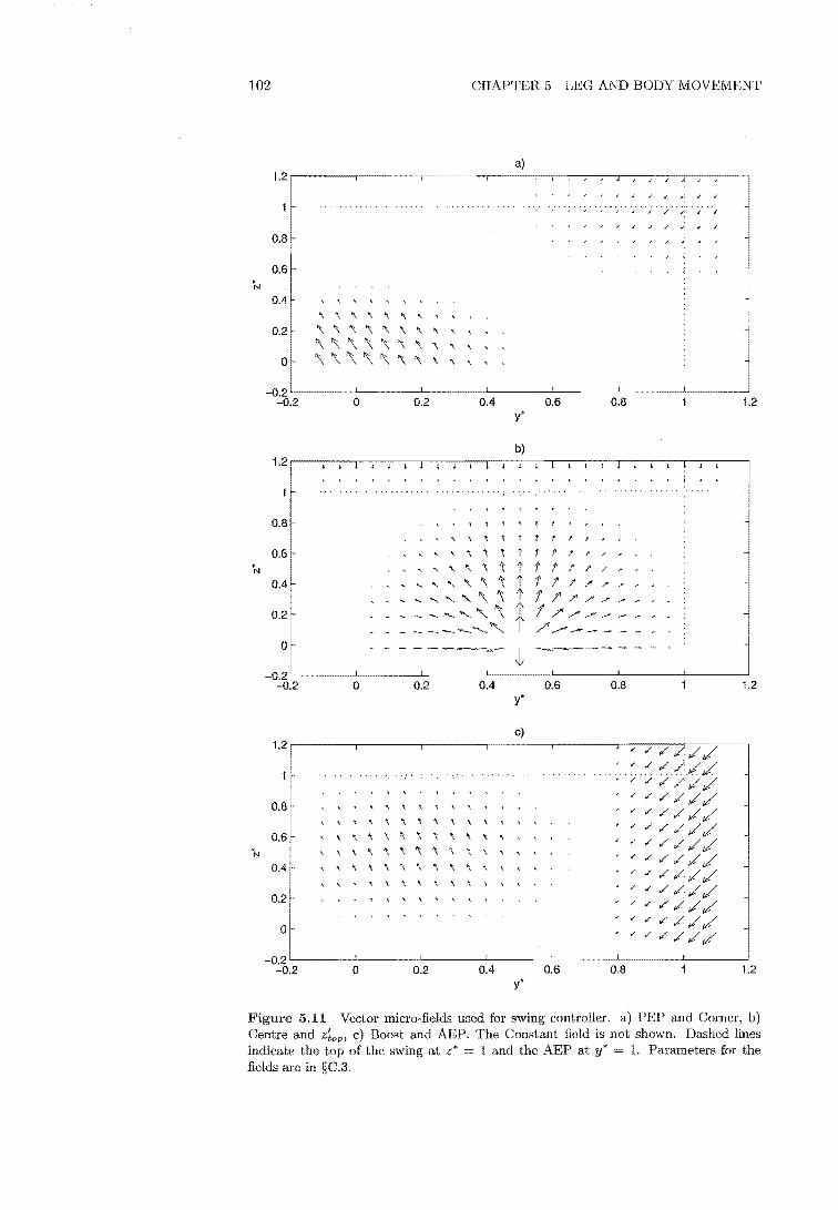
102 CHAPTER 5 LEG AND BODY MOVEMENT

0.8

0.6

0.4

" " " " " " , , , 0.2 '\ '\ '\ '\ '\ '\ '\ '\ , ,

'\ '\ '\ '\ '\ '\ '\ '\ '\ , , 0'\'\\\\'\'\'\'\"

-0.2 '----- _'--___ l -0.2 a 0.2 0.4 0.6 0.8 1.2

y'

b) 1.2~---I--I~I~-'--'--I~I--I---I--,-~j-I--I---I-~!-'--I--,--r-j-I--I--I--I~-I--I---­

i

0.8

0.6

0.4

0.2

a

, , 1: ttl ,

" '\ '\ , t t

",,,"Itt ",'\'\'\tt """,\,t

--""'\'\f ----- ...... ,,'\ -----,

t t t f

rttt" tf't!'/" ttl'//"", tl'/'/'/"", !/'/./.­/'/""----

- - - - ------.-.--- ,t ------_0.2'--------L-----__ ~············ ___ L_ ______ L_ ____ i_ ______ ~ ____ ~

-0.2

0.8

0.6

0.4

0.2

a

a 0.2 0.4 y'

c)

\ \ '\ '\ '\ '\ '\ , ." ." , ." ... '\ '\ '\ '\ '\ '\ '\ '\ '\ , , , , '\ 'I '\ '\ '\ '\ '\ '\ '\ , , ,

, , , '\ '\ '\ '\ '\ '\ '\ '\ , , , , , \ 'I 'I '\ '\ '\ 'I '\ '\ , ,

, ." '\ '\ '\ '\ '\ '\ '\ '\ '\ \

." ." " \ ." "

-0.2 '--______ L_ __ _

-0.2 a 0.2 0.4 y'

0.6 0.8 1.2

0.6 0.8 1.2

Figure 5.11 Vector micro-fields used for swing controller. a) PEP and Comer, b) Centre and z~op, c) Boost and AEP. The Constant field is not shown. Dashed lines indicate the top of the swing at z* 1 and the AEP at y* 1. Parameters for the fields are in §C.3.

5.5 SWING MOVEMENT 103

1.2 " " '" '" '" '- '" '" '- '- '- " " " t IV J J. -- - - -..,;;; ... "- \ \ JJJl

J $ j .j

0.8 J .j

.... " /' I' /' / J j

? -' /' /' I' t t t t I /'//~-J j

0.6 /' " I' I' t t t t t t I /'/./.-J J t t t t t l' t///_'''_~, 'N t J J

0.4: I t t t t t r t t !///-"'--, J J t t t t t , ~ t t t t/'// ______ , , J J

0.2 t t t t ~ , ~ f t / / _________ " \ J J

t t i t , , '\ '\ '\ , t / ___ ~ __ " \ J J

0 t t , '\ - \ ~ -, ~-- -.... " \ J J

-0.2 -0.2 0 0.2 0.4 0.6 0.8 1.2

y'

Figure 5.12 Total swing field and sample trajectories through it.

the parabolic shape. As the leg approaches the AEP it needs to decelerate

and start descending. This is the role of the Corner micro-field. The AEP

micro-field prevents the leg from going past the AEP and makes it descend

steeply to make a footfall. It must overcome the Constant micro-field to

prevent the leg going past y' = 1. The Constant and AEP micro-fields

continue below y* 0 (not shown in Fig. 5.11) so that the AEP can be

lower than the PEP.

The micro-fields in Fig. 5.11 (plus the Constant field) add together to

form the total field in 5.12. The trajectories plotted through the field

start at widely varying points but all converge to the AEP at y* 1,

demonstrating that this field is robust in the face of perturbations. In practice the trajectory always starts at (0,0) because of the definition of

the normalized field, but changes in step length and 0' i during swing can

subsequently move it away from that trajectory towards the others.

5 .6 Step Length Reduction

As described earlier in §5.5.4, changing the step length parameter l~tep al­

ters the normalized position y* so that the leg is earlier or further through

the swing motion.

Equation (5.10) shows that reducing l~tep increases y*. If the reduction

happens during the lift phase the innermost sample trajectory in Fig. 5.12

suggests that the swing apex will be slightly lower. This is not a major

Total field

Reduction ...

... vs. expansion

Continuous and asymptotic

104 CHAPTER 5 LEG AND BODY MOVEMENT

concern. During the extend phase, reducing l~tep might perturb the leg

above y* I, in which case the AEP micro-field pushes the leg back to-

wards y* 1. These examples show that reducing l~tep is feasible because

it leads to desirable behaviour.

Increasing the step length during swing does not work so wen. During

the extend phase an increase in l~tep will cause the leg to rebound if the

perturbation returns it to the lift phase. best option is to have the

step length slightly longer than normally required and to reduce it when

necessary (even as a matter of course) rather than increase it.

If the step length reduction is discontinuous then the position in y* is

also discontinuous and the swing will probably be jerky. l~tep should be

reduced smoothly then, and it should ideally converge by the end of the

swing so that the final descent at the AEP is almost vertical.

R x The restrictedness described in Chapter 4 incorporates all of the influences

on the step length described in §5.5.1. It can be used very effectively to

reduce the step length. Legs should always be restricted to some extent

at the AEP (either close to the anterior neighbour or the edge of the

workspace to have the maximum step length), but if a leg becomes re­

stricted too quickly then the step must be shortened. Determining if the

restrictedness is too high requires a model of how quicldy the leg should

become restricted as it approaches the AEP. If the actual restrictedness is

ever higher than predicted then the step is shortened so that the predicted

and measured restrictednesses converge. The shorter step can be deter­

mined from the actual restrictedness as long as it increases monotonically

towards the AEP: monotonicity means that the inverse function (finding

y* from R;wing) is single-valued.

ax components ignored

aX components used

5.5.7 Restrictedness During Swing

Only some of the restrictedness components reliably indicate the end of

the swing so a special combination of them is needed, R;wing' RX(p.)5

and RX (pI) decrease through the swing and do not determine when it

should end. RX(,) and RX(P) usually increase as the swing approaches

its apex, and then decrease again before the AEP.

5.13 shows the remaining components. RX(a.) and RX(a.f.) are part

of R;wing because they increase monotonically during the swing. RX(r)

and RX (a) usually decrease at the onset of swing but then increase again

5See Table. 4.1 for an explanation of R'" terms.

5.5 SWING MOVEMENT 105

1.2 RX(swing) + RX(r)

+ x R\a) + 0 RX(a.) + RX(a.f.) +

0.8 + + +

>< + a: +

0.6 + + ++

++ 0.4 ++

+++ ++

0.2

0 439.5 440 440.5 441 441.5 442 442.5 443

! (s)

Figure 5.13 Variation of key components of R'" during a typical swing movement. R"'(a./.) and R"'(a) are both close to zero throughout the movement so they appear one on top of the other on the abscissa.

near the edge of the workspace because they are higher at both the AEP

and the PEP than they are near Xi,home' RX(r) and RX(a) cannot be

added directly because R;wing must be monotonic, but they are essential

indicators that the step should be shortened. Recognising that RX(r) and

R x (a) have one minimum each during a swing, they are added into R;wing

only if they are increasing. The black line in Fig. 5.13 shows the sum of

the increasing components of R;wing'

The discontinuity in R;wing leads to jumps in the normalized field po­

sition y* (which is determined from R;wing) and therefore discontinu­

ous velocity. To prevent jumps in the leg velocity the predicted R X

must be larger than R;wing when the discontinuity occurs, because if

R~redicted,swing > R;wing the step is not shortened. Fig. 5.14 demon­

strates this. Using a higher R~redicted,8wing, line a), the discontinuity is

'hidden' and no jump will occur.

5.5.8 Predicted Restrictedness During Swing

Individual restrictedness components are exponential, so a reasonable ex­

pectation is that the restrictedness will generally increase exponentially

as the AEP approaches. The form of the R X predictor is:

RX _ k{y* predicted,S'wing - e (5.14)

Discontinuous

106 CHAPTER 5 LEG AND BODY MOVEMENT

1.2 RX(swing) + RX(r)

+ + + + +

0.8 +

a)

0.6 b)

0.4

0.2

0 439.5 440 440.5 441 441.5 442 442.5 443

t(S)

Figure 5.14 Two possible R~redicted,.wing exponential functions, dashed lines. a) higher function is not exceeded when R"'(r)home starts increasing, b) lower function is exceeded: step length will be reduced and swing velocity will be discontinuous.

The minimum values of RX(r) and RX(a) components during the swing

can be reliably estimated, but the correct y* at the minimum of RX(r)

and RX(a) changes depending on the PEP and linitial,step' It is therefore

difficult to provide a theoretical for the choice of k and YRx=l) and an

empirical choice is necessary that minimizes the chance of a discontinuity . R X In swing'

Directly selecting values for k (exponential rate) and (y* value

where R X 1) is not intuitive. An easier way to design the predicted RX

curve is to specify its value at the AEP, R~EP' and at some other point

Y~ode where R~Tedicted,swing = R~ode' The derivation of (5.15) and (5.16)

are given in §D.1.

YRX=l 1- InR~EP (5.15) k

In ~~EP (5.16) k node

1 Y~ode

(5.15) and (5.16) are used to find an appropriate specification for the

predicted restrictedness, one where there are no (or

the R;wing discontinuity exceeding it.

occurrences of

5.5 SWING MOVEMENT 107

0.8 x a::

0.6

0.4

0.2

+ 0 239 239.5 240 240.5 241 241.5 242 242.5

t (s)

Figure 5.15 Step length reduction when swing is restricted. Measured R X falls at 241.9s because some components stop increasing and no longer contribute. l~tep is normalized to the original step length.

5.5.9 Calculating Step Length from Normalized Position

If R;wing > R';redicted,swing then the controller must reduce l~tep so that

they are equal. Substituting R;wing in (5.14) and rearranging to find the

value of y* where the prediction and measurement match:

R~wing

" In YRx=l + --k--'<- (5.17)

y~ew is the position in the normalized swing field where the leg should be

if R;wing and R';redicted,swing are to be equal. Substituting y~ew into the

equation for the normalized field (5.10) and rearranging to find the new

step length lstep,new:

" Ynew

lstep,new

Y' ,

YPEP

lstep,new , , Y -YPEP

Y~ew (5.18)

The reduced step length lstep,new makes the current foot position Y~ew'

Fig. 5.15 illustrates a typical experimental step length reduction. Note

that l~tep is continuous and asymptotic, indicating that the leg moves

smoothly and that by the time the AEP is reached the step length cor-

Task coordinate system

Swing problems

Swing vector field

Algorithm

AEP targeting

108 CHAPTER 5 LEG AND BODY MOVEMENT

rection is complete.

5.5.10 Summary

The task coordinate system decomposes movements into components or­

thogonal to the referred motion of the robot (x') and components in the

plane of the referred motion (yl and Zl). Incremental stance leg move­

ments can be calculated using the task coordinate system, although there

is little advantage over simply using the rigid body equations.

The exact position of the ideal AEP (the AEP where the subsequent

stance movement passes through X home) cannot be determined without

foreknowledge of the robot's movements. Even if future movements can

be anticipated the solution for the optimal stance trajectory has not yet

been found (see §5.5.11) and the AEP depends on the (unknmvn) topology

of the walking surface. Approximations are therefore appropriate during

swing, and driving x' asymptotically towards zero generally leads to near­

optimal behaviour.

The key difficulties faced when determining the remaining components of

the swing movement (y' and Zl) are that the PEP is extremely variable,

the step may need to be shortened during the swing, and the trajectory

should be smooth. A vector field normalized to the current step length

fulfils all of these criteria, so long as the step length reduces smoothly.

This section explained the technique to achieve that and results were

given.

Fig. 5.16 summarizes the algorithm for determining the desired foot po­

sition at the next time step during a swing movement. y* and are

evaluated from the vector field in Fig. 5.12. Note the parallel pathway for

the calculation of x', emphasizing the independence of movement perpen­

dicular to the x' = 0 plane and within the plane.

Discussion

Some insects display an AEP targeting behaviour that closely correlates

the foot fall with the position of the leg in front of it (§2.4.1). To some

extent the swing algorithm exhibits AEP targeting during forward and

reverse walking. proximity of the anterior neighbour, through the

restrictedness, squashes the vector field causing the swing leg to descend

a short distance from the anterior neighbour. The swing is never extended,

so if the step length is less than than the distance necessary to reach the

5.5 SWING MOVEJ\;IEl\T'}'

x', y', z·

Integrate x\Sl&z'

x', y', z'

Yes

CalClHate· x."

Rswlng,total

No

109

Figure 5.16 Summary of the swing algorithm a normalized vector field. This flow chart does not depict the conversion from the robot coordinate system to O'i and back again.

What happens during turning

Poor behaviour

110 CHAPTER 5 LEG A~D BODY MOVEMENT

Figure 5.17 Convergence to x' 0 during turning does not lead to ideal behaviour.

anterior neighbour there will be no correlation.

For general, omnidirectional, walking AEP targeting is not exhibited be-

cause the AEP is not necessarily close to the anterior During pure

sideways walking the neighbouring legs are very distant, so the restrict­

edness caused by them is insignificant and this coupling is non-existent.

Other components of the restrictedness still increase as the leg extends

laterally and cause the footfall to occur at a suitable location.

For pure rotational body movements the trajectory of the stance legs in

the xv-plane is a circular arc centred on Obody' If X i,home is a point

on this trajectory (i.e. the trajectory passes through the centre of the

workspace), then the circle has radius rhome = VX~ome + y~ome shown in

Fig. 5.17. 5.17 shows that positions (Xi) on the ideal trajectory

do not lie on the y'-axis (Xl 0) calculated from that point: the y-axis

pa.'3ses through Xi,home according to the definition of i (§5.3.2).

From the diagram, when the leg is at an angle () from Xi,home:

d Thome - Ta

and cos () ra

Thome

d Thome (1 - cos ()) (5.19)

d is the distance between the ideal trajectory and the trajectory generated

by the asymptotic convergence to Xl = O. \i\Then () 25° the error is

5.5 SWING MOVEMENT 111

about 10% of r'home, which is quite significant, The y'-axis would be

better located tangent to the ideal trajectory, rather than passing through

X home' If that were the case then converging on x' = 0 would lead to the

optimal trajectory,

To locate the y'-axis on the ideal trajectory, that ideal trajectory has to

be known, perhaps using an estimate of the future movement commands.

Appendix D.2 derives second order differential equations for the ideal

trajectory, which should be solvable but have not been solved yet. An

additional problem is that the current foot position must map to a point

on the ideal trajectory where the y'-axis (whose orientation is found in

the same way as before, §5.3.2) is a tangent. It is not immediately clear

how this point on the ideal trajectory would be found, The would

still pass through X home so that the y' distance through the swing could

be determined. The discrepancy d can be quite large, so the investigation

of these problems is useful future work.

The robot may be stationary when some are swinging. The two causes

of this situation are that legs may be in mid-swing when the robot body

movement stops and that legs might be rearranged when walking begins

(§4.4.3). If the robot is stationary then having the legs return to their

horne positions rather than completing their swing may be more desirable

because the robot ends in a more stable, symmetric configuration. This

can be achieved by setting l~tep to the horizontal distance between the

PEP and the horne position.

Experiments with sideways walking using Hamlet initially proved prob­

lematic. The step length would usually fail to reduce rapidly enough and

the swing trajectory would carry the foot almost underneath the a-joint,

becoming very close to the kinematic singularity. This leg position is of

course one of high restrictedness, but none of the restrictedness compo­

nents triggering the reduction in l~tep are high until the leg is very close to

the singularity (at which time the a component increases rapidly). This

problem was solved by calculating linitial,step depending on the movement

direction, reducing the initial step length to a more sensible value if the

robot was commanded to walk sideways. The full step length was

when there was no sideways movement component, and the two lengths

were blended for movement vectors between forward and sideways walk­

ing.

Future work

Swing movements when stationary

Sideways walking

Obstruction at PEP

Effect of body UloveUlent

Blending

Not near AEP

112 CHAPTER 5 LEG AND BODY MOVEMENT

5,6 Swing/Stance Blending

5.6.1 Introduction

When walking over anything but perfectly flat terrain there is a likeli­

hood that a footfall might sink into the surface or be placed next to an

obstacle. \Vhen making the transition from stance to swing mode at the

PEP the foot must disengage from the surface before it begins its forward

movement. The need for this behaviour was particularly apparent when

Hamlet was walking over a ridged surface covered by soft sand. If the for­

ward part of the swing movement begun without an adequate lift phase

then the feet caught on the and walking was interrupted - this was

the purpose of the PEP field in Table. 5.1 and Fig. 5.11.

The vector field, however, specifies movement with respect to the body

not the ground, and the body frame is usually moving. \Vhile the PEP

field ensures the lift at PEP is vertical in Obody, the body movement

introduces extra, as yet uncompensated, horizontal movement that can

make the feet catch on the environment. Adding explicit compensation

to the vector field for the stance movement does not work because the

body movement rate varies.

Blending the two movements together at the beginning of the swing can

realise the smooth transition from stance to swing. This has the advantage

that it uses the appropriate horizontal stance velocity, compared with

always arranging the swing vector field to point in the -y' direction near

the PEP. For example, if no body movement is commanded (or it is scaled

back because legs are restricted, §4.4.2) then, using blending, the swing

will begin by lifting straight up. A predetermined rearwards movement in

the swing field would drag the foot in the posterior direction in this case.

5.6.2 Blending Functions

5.18 shows the simplest blending functions: linear transitions from

stance to swing over a change in z' of l~lend' kstance and kswing are the

proportions of stance and swing movements contributing to the overall

movement, as functions of z'

blending functions should only be active near the z' - z~ EP is

usually less than l~lend near the AEP as well, but blending should not be

performed when the leg is in the extend mode. Although some roboti­

cists advocate the anticipation of stance at the end of swing, there is no

5.6 SWING/STANCE BLENDING

0.8

0.6

0.4

0.2

o

o 0.005 0.Q1 0.Q15 0.02 z-

0.025 0.03 0.035 0.04

Figure 5.18 Simple swing blending functions, in this graph l~lend .03.

evidenc'e for this behaviour in insects (c.f. §2.2.3).

113

0.045

Fig. 5.19 shows an experimental demonstration of the effect of blending

that successfully prevented the feet becoming stuck at the PEP.

0.01

0

-0.01

-0.02

-0.03 -N

-0.04

-0.05

-0.06

-0.07

-0.08 -0.08 -0.06 -0.04 -0.02 o 0.02 0.04

y'

Figure 5.19 Example of blending stance and swing movements: swing from the PEP on the left-hand side to the AEP. During the initial lift away from the PEP the leg continues with the stance movement, then smoothly transitions into the swing movement. The trajectory is presented in the robot coordinate system.

Over-restriction

Incorrect l~tcp reduction

114 CHAPTER 5 LEG AND BODY MOVEMENT

5.6.3 Restrictedness During Blending

When stance and swing movements are blended the restrictedness gener­

ally continues to increase after the PEP rather than decrease as it does

without blending. One consequence of blending, therefore, is that it can

potentially cause collisions or over extensions where 2': 1. The sim­

plest, albeit not rigorous, solution is to begin the swing at a sufficiently low

R X so that the movement during blending does not lead to R X 2': 1. An

alternative is to make the restrictedness parameters conservative so that

even if R X 2': 1, blending does not cause collisions or kinematic problems.

Hamlet successfully employs the second technique. Other, more rigorous,

methods might be proposed: accelerating the transition to swing when the

restrictedness is high in a manner similar to the reduction of step length

as the AEP approaches (§5.5.6), or correcting the position if R X 2': 1 to

one where R X < 1 .

The second problem caused by blending is that some components con­

tributing to RFotal,swing (§5.5.7) no longer decrease at the onset of swing.

Because these components (namely RX(r) and RX(a)) are generally large

at this time, R;otal,swing > R~redicted,swing and the step length shrinks ac­

cording to the algorithm in §5.5.6. Preventing the l~tep reduction during

blending can easily avoid the error.

6

Modelling Restrictedness

The restrictedness gait controller worked satisfactorily with the empirically

chosen parameter values, but during forward walking the robot took a long

time to converge to desirable step sequences. At low speeds it sometimes

did not converge at all. The halting behaviour was displayed frequently

and the legs did not appear to be cooperating with each other. This chapter

describes a simplistic model of the robot and its gait controller, and the use

of the model to determine the best parameters for rapid gait convergence.

6.1 Introduction

6,1.1 Motivation

Choosing the optimum restrictedness parameters is a daunting task be­

cause of their number and because of the potential for chaotic interactions

between them. Many of the seven restrictedness components have three

parameters (upper and lower limits and a zone size) and they can be dif­

ferent for all six legs. Interaction between components is unavoidable, and

in fact necessary in order to coordinate walking.

Experimental work introduces the added complexities of sensor, environ­

mental and actuator dynamics and unpredictability. In addition, active

COlTIplex system

Experimental optimization

Analytical model

Simulating model

Multiple optima

Chapter outline

116 CHAPTER 6 MODELLING RESTRICTED NESS

compliance and the other non-locomotive behaviours also affect the timing

of mode changes (§5.2). Experimentally determining the optimal param­

eters is practically impossible, even if the intention is only to optimize

walking on hard flat ground.

The system is deterministic and the timing of its events (mode changes)

can theoretically be determined analytically. Optimization could poten­

tially be carried out on a mathematical model rather than through ex­

periment, avoiding some of the problems just described. However, the in­

terdependence of leg restriction with the state of all the other legs makes

the mathematical analysis intractable (or at least exceedingly complex).

Even determining, from arbitrary leg positions, which leg will swing next

is a challenging proposition. Simulating the model is the only practical

way to deal with the system's complexity.

The potential for very non-linear effects on performance and interaction

between component parameters is enormous. Until proven otherwise the

optimal system parameters must be assumed to be strongly interdepen­

dent (i.e. changes in one parameter have an effect on the optimal values

of other parameters). An exhaustive simulation of the complete system

over all the possible parameter combinations is impractical with the num­

ber of variables involved. Fortunately some restrictedness components

have little on the gait optimality so complete modelling is unneces­

sary. Optimizing a simplified model, with the salient parameters affecting

forward walking, can still provide insight into the full system, and that

insight is used to improve the robot's walking efficiency.

The optimum gait depends on the current manoeuvre (for example turn­

ing on the spot or walking sideways) and the walking environment, so

different restrictedness parameters would be expected to provide optimal

efficiency during different behaviours. The optimal system parameters

could be determined by simulating a simplified model for a of

different terrains and manoeuvres, and then the most appropriate param­

eters selected online during the mission (per haps using a fuzzy selector).

However, one of the chief advantages of the restrictedness algorithm is that

it is capable of omnidirectional walking without adjustment: changing the

gait generating algorithm online destroys that advantage.

The next section of this chapter describes a one-dimensional model of

one side of a six-legged robot, called the Basic 3-Legged Restrictedness

Model (B3LRM). §6.3 covers the simulation of the B3LRM. This section

concludes with a short review of some previous models used to find optimal

gait controller parameters.

6.1 INTRODUCTION 117

6.1.2 Review

Simulation and numerical optimization have been used in the past to find

the best parameters for gait controllers. Of these, the most relevant are

those based on the stick insect (c.f. §2 AA).

Dean (1991b) undertook computer simulations in which the four main leg

coordinating influences of stick insects (Cruse, 1990, c.f. §2AA) modified

the 'intrinsic' AEP and PEP of each simulated leg. The AEP targeting

(affecting the AEP), rostrally-directed inhibition of protraction during

protraction by the posterior leg (caudal shift of PEP), rostral excitation

of protraction during retraction of the posterior leg (rostral shift of PEP)

and caudally-directed excitation of protraction dependent on the position

of the anterior leg (rostral shift of PEP) were included. The last two were

also used as symmetric contralateral influences. Some of the influences

were made temporally-dependent to fit with behavioural data, but the

majority were spatial. Qualitatively the model displayed the characteristic

stepping sequence and contralateral asymmetry of adult stick insects.

main problem with this model was (and still is) that there is very

little quantitative information available on the strengths of the coordinat-

influences in the biological systems. As a consequence of the lack of

complete information (or perhaps because the model is incomplete, see

Shortcomings in §2AA), many starting configurations resulted in static

stability violations. Cymbalyuk et al. (1998) attempted to find more

robust coupling strengths that reduced the frequency of falling.

approach used a 'genetic' or 'evolutionary' algorithml for a coarse opti­

mization and then the 'downhill simplex method' 2 to further refine the

parameters. In the best model the home position (Le. centre of each leg's

movement range) varied with speed and the acceleration at the onset of

the walk was limited3 .

Luk et al. (2001) also used a genetic algorithm, to find the most stable

phase relationships for sideways walking by the eight-legged Robug IV's

fixed gait controller.

fundamental idea of genetic and evolutionary computing is to identify the best of many candidate solutions, then mutate or breed the best of them to generate a new generation of similar candidates. Those are in turn bred or mutated, and so on until the optimal solution is found.

2The downhill simplex method is a multi-dimensional optimization algorithm. The current candidate solutions form the vertices of a polyhedron in the input space which is reflected and scaled to find potentially better parameters.

and Waldron (1987) showed analytically that moving the home position of the anterior and posterior leg pairs out improved stability during regular wave gaits.

Simulating Cruse (1990}'s model

Improving stability

One-dim&nsional

Swing termination

R X component equivalents

118 CHAPTER 6 MODELLING RESTRICTED NESS

6.2 Three Leg Restrictedness

6.2.1 Model Description

The Basic Three Leg Restrictedness Model (B3LRM) is intended only to

model forward walking over flat ground. With no sideways or turning

body movement components, the trajectories are always parallel with

the longitudinal axis. Thus in the B3LRM each leg position is a one­

dimensional quantity. The B3LRM ignores the dynamics (i.e. inertia,

coriolis forces), gravity and actuator and sensor behaviour. Each leg has

the same two states as the full restrictedness algorithm (swing and stance)

and uses the same basic algorithm described in §4.2.4:

foreach in Legs {

}

if ( Leg_Mode_Is_Stance and

Leg_Is_Restricted and

AILNeighbours_Modes_Are_Stance ) then

Leg_SwitclL To_Swing_Mode

else if ( Leg_Mode_Is_Swing and

Leg_Is_On_Ground ) then

Leg_Switch_ To_Stance_Mode

However, the B3LRM cannot determine the end of swing (Leg_ Switch_

To_ Stance_ Mode condition) as the robot does because it does not model

the ground. Instead, in the B3LRM the swing mode completes when its

movement reaches a maximum step length lstep,max (measured from the

PEP) or if R X :2: 1. The step length determines the footfall in the robot

implementation but the restrictedness reduces the step length if necessary

(§5.5.6), so the result is basically the same.

B3LRM includes simplifiL'Ci equivalents of the restrictedness compo­

nents from Chapter 4 that had the most impact on forward walking (Ta­

ble. 4.1 and Fig. 4.3 describe all the restrictedness components). Fig. 5.13

and other measurements (not shown) showed that the most important

components are RX(r) (maximum horizontal distance of the foot from

home), RX(a) (physical limits on a joint), and the primary components

measuring the leg separations (R x (a.) and R x (p.)).

RX(r) and RX(a) both have the same effect when the robot walk':! directly

forwards: they limit a leg's rostral-caudal movement relative to its home

10

6.2 BASIC THREE LEG RESTRICTEDNESS MODEL 119

a) b)

Figure 6.1 Explanation of parameters for B3LRM. a) Definition of Tma.x and tlTma.x.

The black circle represents the position of a foot a distance T from its neutral position P hame • The foot's restrictedness (solid line) increases linearly over a distance tlTmax

until R X = 1 at T = Tmax. b) Definition of Ofeet,min and tl0feet,min' Ofeet is the distance between two adjacent feet (black dots again). In this diagram the solid restrictedness line is fixed with respect to the right foot. The restrictedness increases linearly over a distance /:!"Ofeet,min until R'" 1 at O/eet Ofeet,min.

position. The B3LRM combines RX(r) and RX(a) into one field, explained

in Fig. 6.l.a). Each leg has the same rmax and Llrmax , and its own co­

ordinate system centred on its unique Phome' Unlike the omnidirectional

robot where RX(r) is one continuous field, in the one-dimensional model

the anterior and posterior r limits can be identified as separate contribu­

tions. This makes it simple to add only the posterior contribution to the

total RX in stance mode or the anterior contribution in swing mode.

The B3LRM also included components measuring the leg proximity,

shown in Fig. 6.l.b). Like the full restrictedness algorithm, the separation

restrictednesses act equally on both that the separation is measured

between. However, like the full algorithm does, swing mode legs ignore

any contribution from their posterior neighbour and stance mode legs

ignore any contribution from their anterior neighbour. The reason for

this was explained in §4.3.3.

The B3LRM assumes that leg velocities in swing (Xswing) and stance

(xstance) are constant and identical for all the legs. The duration of swing

(tswing) and stance (tstance) , and hence the duty cycle j3, can easily be

related to the leg velocities by (6.1) (l~teP is the actual length of each

step):

j3 = tstance

t swing + t stance (6.1)

The B3LRM must include the halting behaviour described in §4.4.2 be­

cause it is essential for safe walking and it has a significant effect on the

Constant leg velocity

Halting

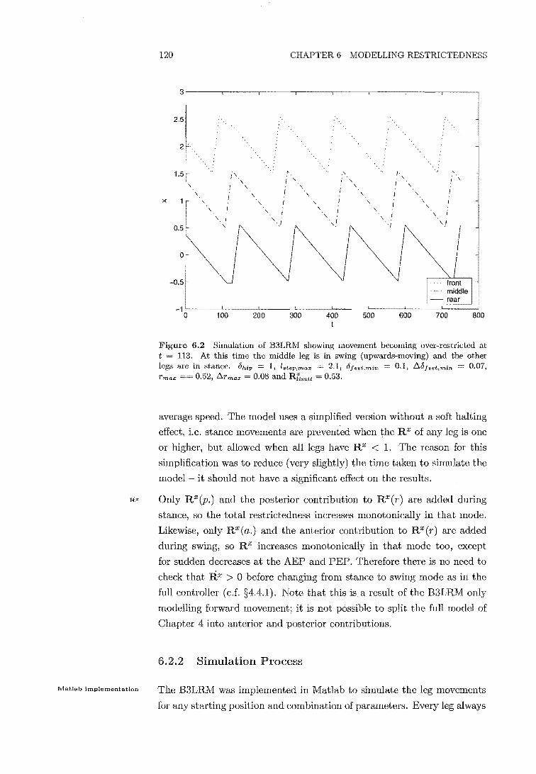
120 CHAPTER 6 MODELLING RESTRICTED NESS

3

2.5

2'

. '

1.5 i'. " .' .'

I , I "

'\ I \

'\ '\ '\ '\

\ '\ '\ '\ , I >< '\ '\ , , \ I , ,

"- "-, I , "- "-I "-0.5 '\

0

-0.5

-1 0 100 200 300 400 500 600 700 800

t

Figure 6.2 Simulation of B3LRM showing movement becoming over-restricted at t 113. At this time the middle leg is in swing (upwards-moving) and the other

are in stance. liMp = 1, lstep,max 2.1, lijeet,min 0.1, l:!.lijeet,min 0.07, r ma", 0.52, l:!.rmax 0.08 and Rli1nit 0.53.

average speed. The model uses a simplified version without a soft halting

effect, i.e. stance movements are prevented when the R X of any leg is one

or higher, but allowed when all legs have R X < 1. The reason for this

simplification was to reduce (very slightly) the time taken to simulate the

model it should not have a significant effect on the results.

R'" Only RX(p.) and the posterior contribution to RX(r) are addE,>d, during

stance, so the total restrictedness increases monotonically in that mode.

Likewise, only RX(a.) and the anterior contribution to RX(r) are added

during swing, so R X increases monotonically in that mode too, except

for sudden decreases at the AEP and PEP. Therefore there is no need to

check that RX > 0 before changing from stance to swing mode as in the

full controller (c.f. §4.4.1). Note that this is a result of the B3LRM only

modelling forward movement; it is not possible to split the full model of

Chapter 4 into anterior and posterior contributions.

Matlab implementation

Simulation Process

The B3LRM was implemented in Matlab to simulate the leg movements

for any starting position and combination of parameters. Every leg always

6.3 STABLE B3RLM PARAMETERS 121

started the simulation in stance mode. Fig. 6.2 shows an example of the

simulated leg trajectories. The trajectories were processed to find the

number of steps by counting the number of changes in the leg velocity.

Other data saved was the number of timesteps where 2:: 1, the time

history of each leg's AEP and PEP and the time taken for the AEP and

PEP to settle close to their final values4 (if they settled at all).

The model parameter Ohip (the distance between the a-joints of ipsilateral

neighbours) is the only B3LRM parameter directly determined from the

physical robot. However, the simulations used Ohip = 1 so that the other

parameters were normalized with respect to it.

The assessment of the model's behaviour must be independent of the ini­

tialleg positions, so every parameter set was simulated for combinations of

four starting positions for each leg. The four starting positions used were

-rmax , and rrrw,x' All combinations were used where at least

one leg started at -r'max (measured relative to each leg's Phome)5. Runs

with the same parameters but different initial leg configurations were ag­

gregated into files containing the mean as well as the best- and worst-case

results, i.e. the mearl, minimum and maximum number of steps, restricted

timesteps and convergence time. Time histories were also recorded for the

mean, maximum and minimum AEP and the same for the PEP.

The first, coarse, search for optimum parameters simulated all 4860 possi­

ble combinations of the parameters in Table. 6.1. Fig. 6.3 shows a dataflow

diagram of the simulation process. The following sections discuss the func­

tions of the two blocks in the assessment part of the diagram.

6.3 Stable B3RLM Parameters

This section examines what the characteristics of a useful gait are and

what simulated parameter values were successful.

lJC.lHlt;U as the time taken until all subsequent AEP and PEP values were within 10% of their final values. The final values used were actually the averages of the last 2% (15 timesteps) of the run, malting the final value more representative in case of small changes in the AEP and PEP near the end of the run.

5This condition eliminates near-duplicate simulations starting with all the legs mov­ing in unison and in stance mode. Simulations without at least one leg at -l'max

show exactly the same behaviour as one that does fulfil that criteria, except temporally shifted (Dean, 1991a).

Normallzed by lihip

Aggregating data

122 CHAPTER 6 MODELLING RESTRICTED NESS

Table 6.1 Parameters for coarse B3LRM simulation.

lstep,max

t5feet,min

.6.15 feet,min {J r'max

.6.Tmax

Maximum step length Min. dist. <-t feet (RX = 1) Ramp distance of 15 feet, min

Leg duty cycle AEP where R X = 1 Ramp dist. of Tmax

RX where

0.51 1.52 0.001 0.2 0.4 t5jeet,min x [0.1 0.51] 0.50.750.95 0.30.450.60.750.9 Tmax X [0.10.5 1J 0.550.750.95

Hard disk

Figure 6.3 Block diagram of simulation process for optimization through modelling.

6.3 STABLE B3RLM PARAMETERS 123

6.3.1 Conditions For

Parameter sets are only acceptable if the AEP and PEP of every leg

settles by the end of the simulation, for all possible starting positions.

This is an 'asymptotically stable' gait pattern that converges to regular

and predictable walking and is robust with respect to its initial state. If

the AEP or PEP don't converge for one or more starting leg configurations

(detected from the worst-case convergence times) then the parameter set

is unsuitable. The final AEP and PEP should not only converge, the value

they converge to must be independent of the leg starting positions. All

the ending AEP (or PEP) values must be within a certain range of the

mean ending AEP (or PEP). The range used for these simulations was

10% of Ohip.

A further condition used for these simulation results was that the mean

AEP and PEP for every leg had to converge on opposite sides of the hip.

This condition might not be desirable for other robots where some legs

are designed to operate primarily caudally or rostrally of their hips. Any

simulation results failing any of these conditions has unsuitable parame­

ters.

6.3.2 Valid Parameter

Fig. 6.4 shows how the six different model parameters in Table. 6.1 in­

dividually affected the likelihood that the trial was good for f3 0.75.

Appendix E includes additional results for f3 = .5 and f3 0.95, with

which comparisons will be made.

One important qualification must be made about interpreting the graphs

in Fig. 6.4. The peaks do not indicate the most optimal values for the

parameters in the sense of efficiency, nor the most robust in the sense of

static stability. The peaks represent values where the gait controller is

most immune to poor choice of the other parameters. Using parameter

values at the peaks gives the controller the highest chance of successful

walking, but it will not necessarily be the most efficient walking. §6.4

covers the determination of the optimal parameters.

Tmax

Fig. 6.4.a) shows that one way to almost guarantee convergence is

to shrink Tmax. The legs will then settle to their final AEP and

on their first steps without any interaction between them. However,

reducing Tmax increases the number of steps required to cover a

AEP and PEP must converge

Not optimal parameters

Small 1'max always converges

124 OHAPTER 6 MODELLING RESTRIOTEDNESS

a) b) 100 100

75

~ j .9

15 15 ~ ~ 50

"tl "tl 0 0 0 0 OJ OJ

25 25

a a 0.3 0.45 0.6 0.75 0.9 0.1 0.5

rmax !J. rma/ rmax

c) d) 100 100

75 75

= f ~ 15 15 ~ 50 C 50

"8 "tl

0 8 VI OJ

25 25

0 0 0.001 0.2 0.4 0.1 0.5

°root,min Ll 0leel,mln I 0reet,min

e) I) 100 100

75 75

f S .9

15 15 C 50 ~ 50

0

"tl "tl 0 0 0 0 OJ OJ

25

0 0.5 1.5 2 0.5 0.75 0.95

Istep,max R~m

6.4 Influence of individual B3LRM model parameters on proportion of good parameter sets. Bars show the proportion of good parameter sets on the ordinate for the different values of the parameter that were simulated on the abscissa. This graph shows the data for (3 = 0.75

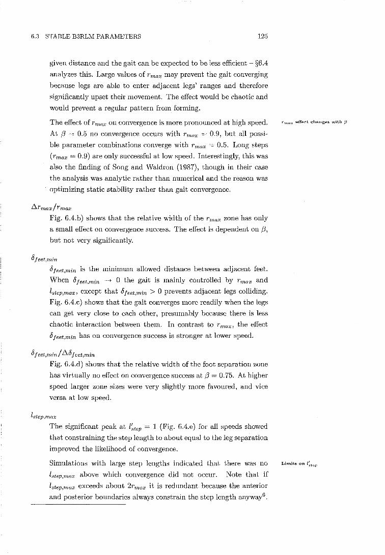
6.3 STABLE B3RLM PARAMETERS 125

given distance and the gait can be expected to be less efficient §6A

analyzes this. Large values of r'max may prevent the gait converging

because legs are able to enter adjacent legs' ranges and therefore

significantly upset their movement. The effect would be chaotic and

would prevent a regular pattern from forming.

The effect of Tmax on convergence is more pronounced at high

At (J = 0.5 no convergence occurs with Tmax = 0.9, but all possi­

ble parameter combinations converge with Tmax = 0.5. Long steps

(Tmax = 0.9) are only successful at low speed. Interestingly, this was

also the finding of Song and Waldron (1987), though in their case

the analysis was analytic rather than numerical and the reason was

optimizing static stability than gait convergence.

LlTmax/Tmax

Fig. 6.4.b) shows that the relative width of the Tmax zone has only

a small effect on convergence success. The effect is dependent on (J,

but not very significantly.

<5 feet ,min

<5 feet ,min is the minimum allowed distance between adjacent feet.

When <5 feet, min -)0 0 the gait is mainly controlled by Tmax and

lstep,max, except that <5feet,min > 0 prevents adjacent legs colliding.

Fig. 6.4.c) shows that the gait converges more readily when the legs

can get very close to each other, presumably because there is less

chaotic interaction between them. In contrast to Tmax , the effect

<5 feet,min has on convergence success is stronger at lower speed.

<5feet ,min/ Ll<5feet ,min

Fig. 6.4.d) shows that the relative width of the foot separation zone

has virtually no effect on convergence success at (J = 0.75. At higher

speed larger zone sizes were very slightly more favoured, and vice

versa at low speed.

lstep,max

The significant peak at l~tep 1 (Fig. 6.4.e) for all speeds showed

that constraining the step length to about equal to the leg separation

improved the likelihood of convergence.

Simulations with large step lengths indicated that there was no

lstep,max above which convergence did not occur. Note that if

lstep,max exceeds about 2Tmax it is redundant because the anterior

and posterior boundaries always constrain the step length anyway6.

rmax effect changes with f3

Limits on

Tripod gait favoured

Early experiments agree

At slow speed ...

126 CHAPTER 6 MODELLING RESTRICTEDNESS

Table 6.2 Effect of {J on convergence with the parameters simulated in Table. 6.1.

0.75 0.95

58.7% 65.7%

sets

The lack of an upper boundary shows that a step length limit is not

essential for gait convergence. Other simulation results (not shown)

indicated that very short l~tep prevented convergence becan.'le the

final convergence values were dependent on the random initial leg

positions: some legs, starting caudally, never made it past the hip.

RUmit Fig. 6.4.f) suggests that RUmit does not have a major effect on the

success of convergence.

6.3.3 Effect of (3 on Convergence

Table. 6.2 shows that walking speed strongly affects the convergence suc­

cess. At (3 0.5 swing and stance durations are similar so the tripod

gait must emerge (§2.3.1). Inter-leg coupling is probably less significant

during tripod gait walking because legs are always ready to swing when

their neighbour finishes its own swing. There is less confusion to drive the

gait away its regular pattern and it may converge more easily.

This observation was borne out by early walking experiments with Hamlet

reported in Fielding and Dunlop (2001). For those experiments the swing

movement rate tracked the stance rate, strongly favouring a tripod gait.

When the fixed duration swing was subsequently introduced (the stance

rate remained variable) the gait controller seemed to become less robust

and much more sensitive to changes in the restrictedness components.

This is an anecdotal observation, but it is consistent with the modelling

results.

On the other hand, at very slow speed legs have not moved far from their

AEP when adjacent legs complete their own protraction, 80 the legs do not

interfere with each other. Convergence is therefore more likely because

there is no chaotic interaction.

6In fact the point where the step length constraint ceases to have any effect in thc B3LRM is lstep,max Tmax - 2ATmax(1 - Rlimit)

6.4 OPTIMAL B3LRM PARAMETERS 127

6.3.4 Valid Parameter Combinations

Although some parameters have strong individual effects on the success of

convergence (i.e. T max , 6jeet,min and l~tep), it is ultimately the combination

of parameters that really deter!llines convergence. Visualizing such a six­

dimensional space is difficult and it is not vital to the determination of

optimal parameters, so it has not been presented.

6.4 Optimal B3LRM Parameters

This· section describes the processing of the simulation data to find the

optimal parameters. Further simulations identified some parameters more

accurately. Only simulations that successfully converged were used (see

§6.3.1).

6.4.1 Optimization Function

The most optimal B3LRM parameter set has the best combination of low

convergence time7 , fewer steps during the simulation, and fewer timesteps

where legs are restricted and movement has to stop. These three measure­

ments must be combined into one overall performance metric determined

from the results of each parameter set simulation. Additionally, there are

mean, best- and worst-case measurements to consider. The worst-case

performance is the most important to optimize, but good mean results

should compensate for slightly less than optimal worst-case performance.

The best-case performance is of little importance.

Each of the three performance measurements in the simulation set (for a

given (3) was converted to normalized values between zero and one:

1 _ Pi - min(p) max(p) min(p)

(6.2)

where Pi is a member of a vector of results p (either the list of mean or

worst-case measurements of convergence times, step count or number of

restricted timesteps). The minimum Pi in each p is the best result and

has Pi = 1.

Some weightings scale the normalized measurements Pi to reflect the rel­

ative importance of the mean and worst-case performance. The weighted

7The largest of the AEP and PEP convergence times is the overall convergence time.

Optimal performance

Normalization

Weightings

Re .. normallzation

1'max important

Optimal 1'mU-T changes with {3

128 CHAPTER 6 MODELLING RESTRICTED NESS

Table 6.3 Best 10 parameter combinations for coarse optimization, f3 0.75.

2 0.75 0.5 0.001 0.5 1 3 0.75 0.5 0.001 0.1 1 0.95 4 0.75 0.1 0.001 1 1 0.75 5 0.75 0.1 0.001 0.5 1 0.75 6 0.75 0.1 0.001 0.1 1 0.75 7 0.6 0.5 0.001 1 1 0.75 8 0.6 0.5 0.001 0.5 1 0.75 9 0.6 0.5 0.001 0.1 1 0.75 10 0.6 1 0.001 1 1 0.95

scores are then added together to create an overall rating for each measure-

ment. The worst-case has twice the importance of the mean in the results

presented in §6.4.2 and §6.4.3. The three (combined) measurements are

similarly weighted and added to produce the overall performance met-

ric. The number of steps was weighted 8.<; five times as important as the

number of restricted time steps and the convergence time.

Lastly, the metrics were normalized again so that the best parameter set

scored one and the worst scored zero. The 1 x part of (6.2) was not

included in this step.

6.4.2 Coarse Optimization

Fig. 6.5 shows the re-normalized parameter ratings for (3 = 0.75 for all pa­

rameter combinations in Table. 6.1. Appendix E provides similar graphs

for (3 = 0.5 and (3 = 0.95. Table. 6.3 lists the parameter values for the

best ten parameter sets.

Tmax

Fig. 6.5.a) shows that Tmax has a strong effect on the rating. The

best six parameter combinations in Table. 6.3 all have Tmax = 0.75.

Similar peak ratings were obtained with rmax from 0.6 to 0.9, sug­

gesting that a range of rmax values provide near-optimal behaviour

if the other parameters are chosen correctly.

At low speed longer steps are possible (also seen in Fig. E.2) and in

fact they tend to have a higher rating because the steps are longer.

Fig. 6.5 only plots the good simulations so the smaller number of

points as rmax increases confirms the observation (from Fig. 6.4.a)

6.4 OPTIMAL B3LRM PARAMETERS 129

a) b)

0 § 0 ~ @ 0 0 0 ~ © § §

0.6 0 0 0.6 8 0

I B 0 8 S §

0 0 0.6 8 0 0.6 § e i OJ 0 OJ

<= 0 c:

~ 0 ~ 0 0.4 9 0 0.4 ; 0 ~

0 § 0.2 0.2 i 0 0

~ 0

8 ; 0 0 0.2 0.4 0.6 0.6 0 0.2 0.4 0.6 0.6

r Ar Ir max max max

c) d)

O. 0.6 i I i 8 0

I (1

I O. 0.6 8 ~ OJ OJ <= <=

~ 0 ~ ~

8 6 o. ® 0.4 ~ I 8 8 @ 0.2

9 ~ 0 0 ~ (1

0.1 0.2 0.3 0

0.4 0 0.2 0.4 0.6 0.6

°leet,min A 0leet,min I 0leet,mln

e) f)

I @ ~ 0 0 §

O.S 8

i I I ~ 8 0

0.6 8 ~ OJ (1 <=

~ 0 § 0.

t;J t;J t;J

~ ; ~ ~ ©

B 0.

~ ~ ~ 0.2

~ 0.5 1.5 2 0.5 0.6 0.7 0.8 0.9

Islep,max R~m

Figure 6.5 Optimal parameter values for B3LRM for (3 0.75. Higher circles are more optimal, having fewer steps, fewer timesteps where the legs are restricted, artd faster convergence.

130 CHAPTER 6 MODELLING RESTRICTEDNESS

that the system is more sensitive with large Tmax. Although fewer

parameter combinations were successful, when they were successful

they were always better than most parameter combinations with

lower Tmax.

I:::..Tmax/ Tmax

ratio of I:::..Tmax to rmax has very little effect on the rating. At

low speed (Fig. E.4) large ~Tmax is slightly better, but at high speed 1'max

(Fig. E.3) there is no discernable preference.

8 jeet,min

High ratings were only achieved with the minimal value of 8jeet ,min

simulated, 0.0018 . This is sensible because the allowable step length

increases as 8feet ,min -+ O. top ten parameter combinations all

had the minimum foot separation so it is the (equal) most important

parameter. The effect was less pronounced at both high and low

speed.

1:::..8feet,min/ 8jeet,min

The relative of 1:::..8 jeet,min to 8 feet, min did not affect the rating

significantly. The first three, second three and third three combi­

nations in Table. 6.3 differ only in the value of 1:::..8 feet,min/ 8jeet,min.

This parameter has the least effect on determining the rating, al­

though there is a consistent (but tiny) preference for the largest

buffer zone size.

Fig. 6.5.e) shows that the step length is equal most important

parameter: all the best combinations had l~tep 1.

Rfimit

Although Fig. 6.5.f) does not show that Rfimit has a strong ef­

fect on rating, Table. 6.3 shows a consistent trend. . larger

.6.8/eet,min (0.5), RX. . = 0.95 was optimal; for smaller b/eet,Tnin hm~t

(0.1), Rfimit 0.75 was best, at least with the optimal Tmax of 0.75.

This suggests that the two parameters must be chosen together be­

cause they are strongly dependent. The choice of one dictates the

choice of other. However, neither parameter is very important

to efficiency.

o could not be simulated because it caused a divide-by-zero error under the particular model implementation used.

6.4 OPTIMAL B3LRM PARAMETERS 131

Table 6.4 Parameters for fine B3LRM simulation.

lstep,max

6jeet,min

f:l6 jeet,min

f3

Maximum step length Min. dist. t-t feet 1) Ramp distance of 6 jeet,min

Leg duty cycle AEP v{here R x 1 Ramp dist. of rmax

R X where

6.4.3 Fine Optimization

- 1.2 in 0.025 increments 0.001 6jeet,min x [110 100] 0.75 0.5 - 1 in 0.025 increments rmax x 0.5 0.95

parameter values in Table. 6.1 are very coarse and probably not very

close to the ideal values. Further simulations were undertaken with the

revised parameter combinations in Table. 6.4.

fine simulations used only f3 0.75 because there was no intention to

give Hamlet the ability to vary walking parameters with speed. f3 0.75

is mid-way between the possible speed extremes.

6.5 and Table. 6.3 show that 6 jeet,min .001 was clearly the logical

and optimal choice for that parameter. Because the ratio -,.-'-"-'="="-'- was

controlled in the rough simulation, and always S I, f:l6 jeet,min was always

very small. For the fine simulation some much larger ratios were included

to see if a large absolute value of f:l6jeet,min had any effect.

f:lrmax had little effect on the coarse simulation at f3 = 0.75. The exponen­

tial field RX(r) (§4.3.2) is equivalent to rmax and f:lrmax in the B3LRM,

but in the full model-RX(r) also provides information required to shorten

the swing movement (§5.5.7). RX(r.) cannot have a very small transi­

tion zone because then it could not reduce the swing length smoothly.

fine simulation used f:lrmax 0.5 because it has a similar shape to

the E for RX(r) that experiments had shown provided smooth step length

reductions.

= 0.95 was slightly more favoured in the coarse simulations than

the other candidates. RUmit close to 1 lifts the legs when they are nearly

completely restricted (at which time they would halt the body movement)

and this was expected to increase the incidence of halting. However,

the optimization function (§6.4.1) penalizes halting and yet still selects

RUmit 0.95 as the optimal value, therefore it was used for the fine

simulation.s.

Shnulation sirn.plified

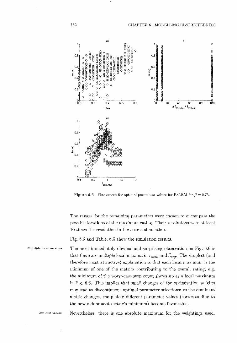
Multiple local maxima

Optimal values

132 CHAPTER 6 MODELLING RESTRICTEDNESS

a) b) 1 §€l 0

O~ 0101 oUo §

0.8 o h i ~ow§· 0.8

OO~ ~ ~~i ~§e 0.6

Ihll~~ul ~8~ 0.6

r:J) 0) c c ~ ~

O. 0.4

~oo 80000 I o 0 0 0.2 o 00 0.2

0 0 I 000 (:'l 0 o 00

0.5 0.6 0.7 0.8 0.9 20 40 60 80 100 rmax Ll. O'eet,min IO,eet.mln

8

0.8

0.6 0) c

~ 0.4

0.2

0 0.6 0.8 1.2 1.4

Istep,max

Figure 6.6 Fine search for optimal parameter values for B3LRM for f3 0.75.

The ranges for the remaining parameters were chosen to encompass the

possible locations of the maximum rating. Their resolutions were at least

10 times the resolution in the coarse simulation.

Fig. 6.6 and Table. 6.5 show the simulation results.

The most immediately obvious and surprising observation on Fig. 6.6 is

that there are multiple local maxima in Tmax and l~tep. The simplest (and

therefore most attractive) explanation is that each local maximum is the

minimum of one of the metrics contributing to the overall rating, e.g.

the minimum of the worst-case step count shows up as a local maximum

in Fig. 6.6. This implies that small changes of the optimization weights

may lead to discontinuous optimal parameter selections: as the dominant

metric changes, completely different parameter values (corresponding to

the newly dominant metric's minimum) become favourable.

Nevertheless, there is one absolute maximum for the weightings used.

6.5 CONCLUSIONS 133

Table 6.5 Best 10 parameter combinations for fine optimization, f3 0.75,

1, Rfimit = 0.95.

Rank Tmax AlJieet,1Ttin l~tep {j [eet,rnin

1 0.825 100 0.875 2 0.85 1 1 3 0.825 10 0.875 4 0.825 1 0.875 5 0.825 1 1 6 0.85 10 1 7 0.875 1 0.925 8 0.825 10 0.975 9 0.825 1 0.975 10 0.85 10 0.9

Table 6.6 Optimal parameters for B3LRM at f3 = 0.75, normalized to 6hip 1.

Symbol Description B3LRM Hamlet

lstep,max Maximum step length 0.875 0.222 8jeet,min Min. dist. +-t feet (RX 1) 0.001 0.09 b.8jeet,min Ramp distance of 8 jeet,min 0.1 0.04 Tmax AEP where RX 1 0.825 0.209 b.Tmax Ramp dist. of Tmax 0.4125 0.1

R X where 0.95 0.95

The area around Tmax = 0.85 contains all the highest rated parameter

combinations (Table. 6.5). The other parameters, b.8jeet,min and l~tepl

are more difficult to pick. Although = 100 is the most optimal

value it does not reappear in the top ten. 0.875 is the most optimal

value but 1 (which is several intervals different) is the second-most optimal

value. -r~=;!!. still proves insignificant in determining the ranking (e.g.

exclude the second row and the top three parameter combinations differ

only in the third column). The very best step lengths (again excluding

the second line) are all 0.875; there are also some near 1 or 0.975 and a

few values in between.

6.5

The optimal parameters in Table. 6.6 cannot be directly transferred to

Hamlet because the B3LRM is quite different to the restrictedness scheme

described in Chapter 4. The main differences are that many restricted­

ness components on Hamlet have no equivalent in the B3LRM, and that

the B3LRM uses linearly-increasing R X functions while Hamlet uses ex-

Hamlet's parameters

Unoptimized parameters

Improvement

134 CHAPTER 6 MODELLING RESTRTCTEDNESS

ponential functions.

However, the optimization results can be used as a guide to select the

functions and other parameters most likely to affect walking efficiency.

The fourth column of Table. 6.6 shows the parameters implemented on the

robot for the experiments described in Chapter 4. Most of the parameters

were simply scaled for Hamlet's 6hip of 200mm. The difference in the foot

separation of the B3LRM and the robot is because experiments showed

that O.09m was the minimum value that prevented the legs from colliding.

This was due to the extremely simplistic modelling ofthe distance between

the legs, which didn't take into account the volumes of the parts. Rl1mit

is identic~l in the model and the real robot. Appendix C lists the the

walking algorithm parameters.

The optimized parameters gave better performance than the initial pa­

rameter guesses for forward walking and to some extent for manoeuvring.

Before parameter optimization the regular periodic gaits usually did not

appear at all, although omnidirectional walking was successfuL The pa­

rameters at this stage were designed to maximize the leg movements by

closely reflecting the physical constraints on them, and were different from

those used by Fielding et aL (2001). main problem with the unop­

timized parameters was that the middle legs usually took two steps for

everyone that the anterior or posterior legs took. The middle legs' step

length was much less than the other and the body frequently halted

while restricted legs waited to change modes.

vVith the parameters in Table. 6.6 the robot displayed dramatically im­

proved gait convergence and all legs stepped with the same frequency

(for straight line walking). The top speed increased considerably because

the body movement did not have to wait for restricted except at

commanded speeds beyond the maximum average velocity of the robot.

A comparative study between the two parameter sets was not felt to be

necessary because the modelling results comprehensively described the ef-

the major parameters have on walking efficiency and smoothness, at

for the modeL

7

Conclusions

This chapter summarizes the restrictedness gait controller consisting of

step sequencing and swing movement algorithms) and the work completed

in the course of developing and demonstrating the system. The first sec­

tion summarizes the dataflow in the algorithm) especially drawing atten­

tion to the interaction between the restrictedness and the attitude control.

General notes are given on obtaining optimal efficiency with the restricted­

ness controller. The second section compares the restrictedness controller

to previous gait controllers, while the third contains suggestions for future

work to extend the controller's capabilities.

7.1 Algorithm Summary

Restrictedness derives from evidence of specific influences observed and

measured in biological systems during forward walking, but expands those

ideas to cope with the more general case of omnidirectional walking.

restrictedness for each leg is a composite of several components, each

representing a physical movement limitation. During forward walking

the most significant restrictedness components correspond approximately

with known inter-leg influences in insects.

Restrictedness is used to decide when to change legs from stance to swing

mode (step sequencing) and also in order to prevent swing movements

Restrictedness

." and Its use

Relevant fix factors

Isolating relevant fix

136 CHAPTER 7 CONCLUSIONS

colliding with other or mechanical limits (swing controller). A task

coordinate system for each leg, dependant on the commanded body move­

ment, greatly simplifies the specification of a velocity field for swing move­

ments and permits omnidirectional walking. Active compliance, a ground

contact maintaining behaviour, and automatic attitude and height control

all contribute to the system's rough terrain abilities.

7.1.1 Merging Attitude Control and Restrictedness

In order to distinguish between worsening and improving restriction, the

algorithm described in Chapter 4 must detect when each leg's restricted­

ness increases in stance mode (c.f. §4.4.1). However, only the restricted­

ness change due to locomotive movement is relevant to this decision, and

any increases due to non-locomotive movement must be ignored. Attitude

and compliance control (the non-locomotive movements) can increase a

leg's restrictedness over the short term even when it is generally decreas­

ing due to the locomotive movement. For example, when a swinging leg

reaches the ground the attitude controller uses the new ground contact

information to move all the legs. The adjustment might increase one or

more leg's restrictedness and trigger its switch to swing mode, possibly

even the leg that just completed its swing. The increase in restriction

due to the attitude correction can be more than the decrease due to the

locomotive movement.

In §4.4.1, Jix was calculated by taking the difference between the R X

calculated at successive timesteps. This simple arrangement includes the

undesirable contributions of the attitude control in Jix. Either R x must be

calculated directly from the differentials of the restrictedness components

and the locomotive movement rates, or else calculated both before and

after the locomotive movement to isolate the relevant contribution. The

second option is by far the easiest to implement, and it should require no

more overhead than the first.

7.1.2 Dataflow

Fig. 7.1 shows the high level dataflow diagram for a timestep of the re­

strictedness gait controller. Circles represent data transformations, double

horizontal lines are storage, and arrows show flows of data from one en­

tity to another. Two additional conventions have simplified the diagram:

encompassing circles indicate data transformations repeated individually

for each leg, and the semi-triangular shape signifies dependence on the

7.1 ALGORITHM SUMMARY 137

commanded leg positions, Xc (XC has been removed for clarity). Dashed

lines are dataftows of data stored from the previous timestep .

. Note that in Fig. 7.1 the locomotive stance movement is calculated in

the task coordinate system. The diagram shows both stance and swing

movements calculated for every leg and the appropriate result chosen by

the multiplexer at bottom right. For efficiency only the required precursor

calculations should be carried out in practice, depending on the actual leg

mode.

7.1.3 Energy Efficiency

Efficiency is important for any device intended to operate remotely or au­

tonomously. In general, biologically-inspired walking controllers cannot

provide any assurance of their optimality in the sense of energy consump­

tion for a given traversal (the 'specific resistance" Marhefka and Orin,

1997). Nature ensures maximum long term efficiency because the evo­

lutionary process of survival of the fittest guides the mechanical as well

as the innate behaviour of animals. However, there do not appear to be

mechanisms or control processes ensuring local optimality of all move­

ments in insects, only rules that generate near-optimal behaviour most of

the time. This is in stark contrast to engineering approaches which often

optimize every movement using criteria directly related to efficiency.

Evolutionary processes (i.e. genetic algorithms) can be applied to

biologically-inspired controllers to evolve optimal designs (potentially in­

cluding the restrictedness algorithm, see §7.3.1). However, Marhefka and

Orin (1997) described five heuristic rules that significantly improved a

simulated walking robot's power consumption and yet were easy to im­

plement. Their rules are relevant to Hamlet and similar robots employing

DC servo motors:

1. Use the largest possible movement velocity, which increases power

but decreases the specific resistance.

2. Use the lowest possible body height, lifting the [-joint above the

{i-joint if possible.

3. Have the tibia vertical at the middle of the stance movement.

4. Share the load amongst as many legs as possible by having fast

swing movements (maximum duty cycle) but don't saturate the

actuators.

No explicit optimization

Optilnization beuristics

138 CHAPTER 7 CONCLUSIONS

Figure 7.1 Dataflow diagram of a single timestep of the restrictedness gait and move­ment controller. Note the Key at middle left and that dashed lines indicate data re­tained from the prcviolliJ timcstep.

7.2 SUMMARY 139

5. Small and large step lengths increase specific resistance. Large steps

decrease the stability margin and therefore greatly increases power

consumption in some legs.

The task control level implements the first two rules so they are not rel­

evant to this discussion of the gait controller. The second rule should

be particularly effective with Hamlet because the assisting springs sup­

port the robot's weight in this configuration (c.f. Fig. 3.4). Appropriately

selecting the leg home position X home achieves the third rule, while cor­

rectly scaling the swing movement's vector field ensures that the duty

factor is high in order to follow the fourth rule. The fifth rule should

not be necessary if other augmentations to the scheme ensure a minimum

stability margin.

7.2 Summary

7.2.1 Work Completed

The following tasks were completed:

1. Constructed a new 13kg hexapod robot, Hamlet, from scratch, in­

cluding virtually all mechanical, electronic and software compo­

nents.

2. Constructed an experimental environment for the robot.

3. Extensively surveyed recent and historic research on the biological

systems that coordinate insect walking.

4. Developed a new interpretation of the principle behind the biological

systems.

5. Developed a powerful yet simple new paradigm for hexapod step

sequencing called 'restrictedness'.

6. Implemented and tested the restricted ness concept on Hamlet, ob­

taining better results than many far more complicated controllers

reported in the literature.

7. Developed a new, improved, method of generating swing trajecto­

ries.

Applicability of heuristics

140 CHAPTER 7 CONCLUSIONS

8. Implemented several important additional behaviours helping the

robot walk over rough ground (active compliance, ground following,

levelling) .

9. Modelled the gait controller and used that model to optimize the

controller parameters for forward walking.

7.2.2 Capabilities and Advantages

The restrictedness concept led to the development of a new step sequenc­

ing algorithm and a new swing controller, together called the restrict­

edness gait controller. This gait controller has a number of important

capabilities and advantages over controllers previously described in aca­

demic literature.

Free gait Free gaits are vital for safe manoeuvring, walking on rough ground

(where footfalls may be delayed or absent) and when starting to

walk, so controllers that exhibit free gaits are an active research

topic. Unlike endogenous oscillator (§1.3.3) or fixed gait controllers

(§1.3.2), the restrictedness controller generates reliable free gaits.

Wave gaits

The periodic metachronal wave gaits used by insects are efficient and

safe, and hence their use is desirable for robots walking forward over

relatively flat ground. The restrictedness controller uses the proper

wave gaits when it can, whereas many rule-based gait controllers

(§1.3.4) that implement free gaits require separate controllers for

wave gaits and for free gaits.

Omnidirectional

Omnidirectional walking is an important capability for walking

robots because they may have to position and orient themselves

in confined spaces. Hamlet's reliable omnidirectional walking capa­

bilities exceeded those of all distributed gait controllers reported in

§1.3.6 as well as most other controller categories, because omnidi­

rectional walking was an explicit goal.

Low computational burden

Despite the exponential growth of computer power, simple algo­

rithms with a low computational load are always preferable to

complex ones that search through a large number of similar plans

7.2 SUMMARY 141

(c.f. §1.3.5). The full system implemented in C (including step se­

quencing, active compliance and levelling, leg movement, kinematic

transforms, joint control, signal conditioning etc) took an estimated

100,000 operations per timestep a mere 17,000 per Unlike gait

controllers that search for optimal plans, increasing the number of

potential movement directions (Le. omnidirectional walking) does

not increase the computational load. The load is relatively constant

because there is no plan/execute partitioning, i.e. it does not plan

moves before spending many timesteps simply executing them.

Simple implementation

For all its capabilities, the restrictedness controller is extremely

pIe to implement in conventional realtime software. It needs only

basic mathematical library functions, it can be arranged in indepen­

dent stages in many possible ways, and it has clear dataflows (c.f.

Fig. 7.1). Some other algorithms build extensive data structures in

memory (requiring dynamic memory allocation which is dangerous

in realtime software) or require concurrent processing (e.g. neural

networks).

Parallel processing

Legs operate very independently in both the restrictedness step se­

quencing and swing controllers and therefore separate processors

can control each leg. The restrictedness depends only on the mode

and instantaneous position of each leg and its neighbours. Although

individual data must be aggregated at some points in the algorithm

(for example halting requires all R X values and attitude control is

centralized, c.£. Fig. 7.1), strict synchronization is unnecessary; in

fact in principle the different leg controllers could run with different

update rates. This sort of flexibility may be useful where reliability

is mission critical because the system could reconfigure itself after a

processor failure, for example running two legs on one processor at

a slower rate.

Easily adaptable

Because physical equipment limitations determine most of the re­

strictedness components the controller is easily tuned for new or

modified robots. Adaptation is simple, especially compared to neu­

ral controllers which might have to be retrained in similar circum­

stances. The controller is built on a basic kinematic software layer

that should have a similar interface across different robots, further

simplifying the migration. The physical ba.sis also means that legs

Summa.ry

142 CHAPTER 7 CONCLUSIONS

(when their designs are identical) share many of the same restrict­

edness components.

Reactive

The restrictedness controller reacts to the robot's situation in the

real world rather than the expected state in a simplified model world.

Both the new gait sequencing and the new velocity field swing con­

trollers easily handle discrepancy between the expected and actual

footfall instants, which usually differ wildly on rough ground. The

deliberative gait planners require planned swings to complete before

attempting the next pha . .''le of the plan and stop until they are com­

plete, whereas the restricted ness controller continues to move unless

the move compromises stability. The new controller reacts instantly

to loss of ground contact to regain its footing.

Full work space model

When walking over very rough ground, particularly manoeuvring on

it, may become overextended or cramped by their joint limits

in unusual ways. For example, a leg stepping on a large rock might

reach its ,a-joint limit before it is halfway through stance, i.e. a long

way from its usual forward or rearward extremes. The gait plan­

ners reviewed in §1.3 have only simple notions of the leg workspace

(for example cubic or even 2D rectangular shapes), and therefore

those workspaces must be conservative to preclude joints reaching

their limits on extreme terrain. In comparison, the restrictedness

components provide a full workspace model so that the legs lift only

when they really need to. The swing controller uses the same full

workspace model, ensuring that steps are as long as possible.

In summary, the restrictedness can choose which legs to lift and also guide

the swing movements. The resulting system is extremely capable, simple

to implement, computationally light and adaptable. It has advantages

over all of the systems so far reported in the literature. The present

research has not seen the implementation of a number of key capabilities

of other systems, but there is no reason why they cannot be added in

the future. Presently the major limitation is an inability to walk on

rough ground, although the active compliance and automatic levelling are

an important basis for this capability. The concluding section describes

the limitations and how they could be added to the basic restrictedness

system.

7.3 FURTHER WORK 143

3 Further Work

The experiments with Hamlet suggested several simple improvements and

extensions to the restrictedness concept that would improve its perfor­

mance or add additional capabilities. One of the biggest advantages of

the approach proposed in this work is that many significant improvements

can be made quite easily because they can be built 'on top of' the exist­

ing software. This section describes additions to the ba.sic algorithm that

would enhance the robot's capabilities.

7.3.1 Minor Extensions

Although Chapter 6 extensively investigated the effect that some restrict­

edness parameters have on walking efficiency, biological systems have ad­

ditional inter-leg influences specifically encouraging efficient stepping se­

quences (c.f. §4.2.3). Augmenting the restrictedness algorithm with simi­

lar behaviours could therefore be expected to improve walking. One way

to augment the algorithm could be to modify Rf based on the positions

of the ipsilateral and contralateral either by scaling it up or down,

or by adding some more inter-leg restrictedness components.

Fig. 7.2 shows the rapid change from one gait pattern to another at differ­

ent speeds when 20% of the anterior neighbour's R X was added to every

leg's RX. This addition corresponds with the protraction excitation by

anterior neighbours in stick insects described in §2.4.3. Changes between

different gait patterns at different speeds were much slower without this

added influence, and the convergence to periodic gaits from standing was

also more rapid than for the results presented in Chapter 4. These are ex­

citing preliminary results and further investigation is definitely warranted.

Hamlet often had difficulty attaining a periodic gait, especially at low

speed, because the swing of rear (or sometimes front) legs often disturbed

the rostral stepping sequence on the contralateral side. Proper contralat­

eral coupling may stabilize the gait by adjusting the contralateral phase

so that both caudal (or rostral) legs were not trying to swing at the

same time. Coupling a portion of the restrictedness from the contralat­

eral neighbour (as was just described for the anterior neighbour) may be

an effective approach.

The optimization process covered in Chapter 6 was extremely success­

ful but it used a very simplified and in some ways inaccurate model. It

would be worthwhile to improve the B3LRM by using exponential func-

Convergence

Contralateral coupling

B3LRM

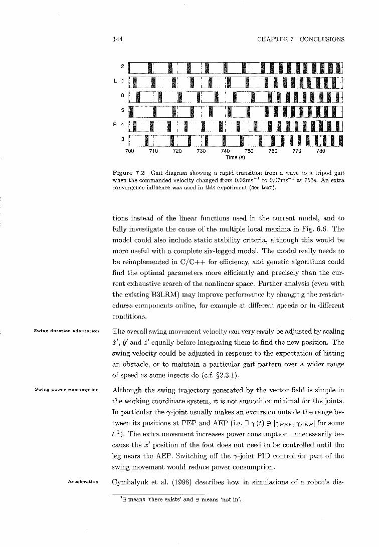
Swing duration adaptation

Swing power consumption

Acceleration

144 CHAPTER 7 CONCLUSIONS

2

L

0

5

R 4

3

700 710 720 730 740 750 760 770 780 Time (s)

Figure 7.2 Gait diagram showing a rapid transition from a wave to a tripod gait when the commanded velocity changed from O.02ms- 1 to O.07ms-1 at 755s. An extra convergence influence was used in this experiment (see text).

tions instead of the linear functions used in the current model, and to

fully investigate the cause of the multiple local maxima in Fig. 6.6. The

model could also include static stability criteria, although this would be

more useful with a complete six-legged model. The model really needs to

be reimplemented in 0/0++ for efficiency, and genetic algorithms could

find the optimal parameters more efficiently and precisely than the cur­

rent exhaustive search of the nonlinear space. Further analysis (even with

the existing B3LRM) may improve performance by changing the restrict­

edness components online, for example at different speeds or in different

conditions.

The overall swing movement velocity can very easily be adjusted by scaling

x', il and 1:;' equally before integrating them to find the new position. The

swing velocity could be adjusted in response to the expectation of hitting

an obstacle, or to maintain a particular gait pattern over a wider range

of speed as some insects do (c.f. §2.3.1).

Although the swing trajectory generated by the vector field is simple in

the working coordinate system, it is not smooth or minimal for the joints.

In particular the ,-joint usually makes an excursion outside the range be­

tween its positions at PEP and AEP (i.e. :3 ,(t) :3 [,PEP, ,AEP] for some

t 1). The extra movement increases power cOIlSumption unnecessarily be­

cause the x' position of the foot does not need to be controlled until the

leg nears the AEP. Switching off the ,-joint PID control for part of the

swing movement would reduce power consumption.

Oymbalyuk et al. (1998) describes how in simulations of a robot's dis-

1:3 means 'there exists' and "3 means 'not in'.

7.3 FURTHER WORK 145

a) b)

Figure 7.3 The home position of the legs supporting the robot (dashed lines) must change when walking on a slope. a) shows the robot on a slope with the standard foot positions; b) shows more stable leg positions after adjusting for the underlying slope.

tributed gait controller based on the model of Cruse (1990) (c.f. §2.4.4) ,

rapid acceleration led to falls in 70% of arbitrary starting leg configura­

tions. (In fact stability was not guaranteed by the controller at all: even

with slow acceleration there was a 10% chance of a random starting con­

figuration leading to a fall.) On the other hand, the restrictedness gait

controller stops its movement to prevent falling, leading to jerky initial

progress but similarly increasing average speed (c.f. Fig. 4.6). Although

the restrictedness algorithm always produces the maximum stable average

acceleration, limiting the acceleration would smooth out the initial surges.

Major Extensions

Some more complex improvements could add important new capabilities

to the basic algorithm.

One of the most clearly needed enhancements is robust handling of prob­

lems with the swing movement, for example when a protracting leg hits

an obstacle or fails to find a footfall because of a ditch or hole. Sensors on

the legs could detect obstructions, whereas a missed footfall is indicated

when 2:: 1 before the foot registers contact with the ground. In these

situations insects initiate rapid searching movements looldng for a new

foothold or, if that fails, change direction (§2.2.3). This is an essential

behaviour that would be needed for practical robot applications. Further

revision of the vector field approach in order to improve the optimality of

its trajectories during turning was discussed in §5.5.11.

Fig. 7.3 illustrates that the supporting legs must generally remain under­

neath the robot when it walks up a slope. A similar situation exists for the

roll axis when walking across a slope. The current work has not addressed

the slope stability problem and consequently Hamlet had difficulty walk-

Robust swing movements

Slope.walking & stability

Slope-walking improvements

Precision stepping

146 CHAPTER 7 CONCLuSIONS

ing on hills in fact, as mentioned in §4.6.2, stability wa.") not guaranteed

even on flat ground. Inhibiting protraction of heavily loaded legs, a la in­

sects, would improve stability in both these situations. However, effective

slope-walking requires additional changes to the restrictedness algorithm

to encourage the legs to operate around the modified horne positions lying

on the dashed lines in Fig. 7.3b).

The changes would, in principle, be simple to implement. Recall from

§4.3.2 that RX (1') models a constraint due to the ,6-joint's torque capability

and that it is nominally calculated from the a-axis. Hence the centre

of RX(1') is currently fixed for each leg, but it could easily become a

function of the body orientation to maintain it more or less underneath

the relevant hip as the body pitched and rolled. If the home position was

moved similarly then the legs would then operate around this new centre

while the other restrictedness components continued to ensure that the

joint ranges and minimum leg separations were respected. Measuring

RX(1') from the dashed lines in 7.3b), instead of lines in a), would

actually be more consistent with the original intent to incorporate the

torque constraint into the restrictedness concept. The consequences of

this change would be far-reaching however: the movements might

have to change on slopes and other restrictedness components would still

limit the workspace.

The ability to choose ground contact points distinguishes walking from

wheeled and tracked locomotion and is important in some environments

(§1.1.1). Although the velocity field method generates adaptable and ro­

bust (to initial conditions) swing movements it cannot easily be extended

for precision stepping. However, for precision stepping the footfall point

is known, which removes one motivating factor behind the velocity field.

The robot could use an explicit trajectory instead of a velocity field for

precision stepping, but would have to plan the swing trajectory to avoid

other legs.

Humans walking on flat ground do not think about where to step, but

over very rough ground they consciously or unconsciously choose their

footfalls. This biological ba.sis is a suitable model for the walking robot:

choose footfalls and calculate trajectories to achieve them when the sit­

uation demands precision stepping, but otherwise use the velocity vector

field. Such a system would be simple to add to the restrictedness gait con­

troller after developing the precision step planning and perception.

gait planning would retain its omnidirectional and efficient forward walk­

ing properties at all times, but the robot could recruit extra processing

7.3 FURTHER WORK 147

Table 7.1 Some potential expansions of the Hamlet project and who, at the Univer­sity of Canterbury, might undertake them.

)cactl(m-tn1.c~ang system AI for navigation Perception systems Natural language user interface Continued robot control development

Elec. Eng. or Compo Sci. Elec. Eng. or Compo Sci. Compo Sci. and/or Linguistics Elec. Eng. or Mech. Eng.

power to help select footfalls when the ground became difficult to traverse.

Precision stepping could also plan footfalls in anticipation of obstacles.

7,3.3 System Improvements

Hamlet continues to operate but some technical issues remain. Of these

the most pressing is the slipping bevel gears mentioned in §3.4.1, which

could be solved by replacing the plastic gears with metal ones.

When insects walk over extremely rough ground their leg spines or other

leg parts often support the animal's weight, not the tarsi (Delcomyn et al.,

1996). Likewise, when walking over rocks Hamlet's femur and protective

carbon fibre boot around the ,-joint motor (Fig. 3.5) often contacted the

ground before the foot. This prevented walking because the load cell did

not detect the ground contact, although in fact the support was sufficient

to have allowed the robot to scramble over the obstacle. Insects detect

ground contact in the coxa rather than just the tibia, letting them use

any part of the for support when scrambling. Future robot designs

should provide spikes on the tibia to catch on rocks and branches, have a

robust tibia and femur to support the robot when scrambling, and detect

contact near the hip. These improvements could be retrofitted to Hamlet,

or on the other hand the restrictedness algorithm could easily by trans­

ferred to other hexapods or even robots with eight or more Note

that the robot would have to distinguish between good (supporting) and

bad (obstructing) contact and then act appropriately, and that the active

compliance behaviour would be affected.

At the time of writing a student, Anna Bonerandi, is attempting to mi­

grate the electronics to a realtime PC framework, using the RTX exten­

sions for Windows NT.

This work provides an exciting and practical platform for developing re­

lated technologies at the University. Table. 7.1 lists seme interesting areas

Mechanical improvements

Ground contact

Control by PC

AI capabilities

148 CHAPTER 7 CONCLUSIONS

of research and departments that might be interested them.

In conclusion, an 18 d. oJ walking hexapod was designed and built and

a novel algorithm has been developed and successfully tested, The system

has been shown to out perform existing gait controllers for a wide range

of conditions. A number of papers have been p'ublished on the work and it

has led to several interesting avenues for further research.

A

Quick Reference

This appendix contains a diagrammatic quick reference sheet for the major

terms used in this thesis.

151

.. Caudal Rostral ----.,..,

Figure A.l Definitions of directions and terms indicating relative position used in this thesis. In this diagram the robot movement is to the right.

Swing/Protraction

PEP ~:;~ AEP

Stance/Retraction

Figure A.2 Relationship of leg movement phases and transition points. The arrow on the trajectory shows the direction of foot movement through the cycle, clockwise in this diagram.

Contralateral On the other side (e.g. the left front leg's contralateral

neighbour is the right front leg).

Ipsilateral On the same side (e.g. the left middle leg's ipsilateral neigh­

bours are the left front and left rear legs).

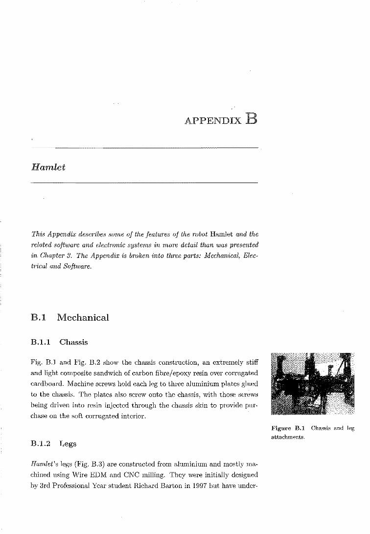
APPENDIX

Hamlet

This Appendix describes some of the features of the robot Hamlet and the

related software and electronic systems in more detail than was presented

in Chapter 3. The Appendix is broken into three parts: Mechanical, Elec­

trical and Software .

. 1 Mechanical

B.l.l Chassis

Fig. B.1 and Fig. B.2 show the chassis construction, an extremely stiff

and light composite sandwich of carbon fibre/epoxy resin over corrugated

cardboard. Machine screws hold each leg to three aluminium plates glued

to the chassis. The plates also screw onto the chassis, with those screws

being driven into resin injected through the chassis skin to provide pur­

chase on the soft corrugated interior.

. 1.2 Legs

Hamlet's legs (Fig. B.3) are constructed from aluminium and mostly ma­

chined using Wire EDM and CNC milling. They were initially designed

by 3rd Professional Year student Richard Barton in 1997 but have under-

B.l Chassis and leg

attachments .

154 APPENDIX B HAMLET

Aluminium Fitting Screw

- Carbon Fibre & Resin

Figure B.2 Chassis cross-section showing corrugated internal structure and attach­ment of aluminium fittings.

Leg attachment

Coupling

Coxa~

Bevel gears

Coupling

__ -libia

Protective boot

/ Force sensor (hidden)

Tarsus

Figure B.3 Design and features of Hamlet's legs. See Fig. 3.5 for joint axis defini­tions.

B.l MEOHANICAL

Femur or Tibia

Coupling insert

Bearings

Gear

Gear shaft

155

Motor

Gearbox

Bearing holder

Motor shaft clamp

Figure BA Exploded diagram of the Oldham coupling between the motors and gears, for [3- and I-joints.

gone many revisions to improve the couplings and reduce backlash. The

complicated femur and coxa designs were necessary in order to have ev­

ery joint on the leg plane, which reduces bending loads on the segments.

Holes and channels reduce the weight of the segments and provide paths

for cables to the motors and force sensor.

Fig. B.4 shows further detail of the steel and brass Oldham couplings join­

ing the motors and gears. A similar coupling exists in the a-joint. Oldham

couplings allow a small misalignment between the motor and gearboxes

axes that is inevitably introduced during manufacturing, but theoreti­

cally introduce no extra backlash. In practice the couplings introduce

some backlash because they must be a sliding fit.

B.L3 Foot Force '-Iv .... "' .......

The foot force must be measured for the non-locomotive movements (§5.2)

and to detect when the make contact with the ground. The sensor

on each foot (Fig. B.5) measures the force in all three directions while

the ball-joint between the load cell and the foot ensures the sensor is

insensitive to torque. Small amplifiers located on the load cell boost the

signals close to their source to provide optimal noise performance (noise on

the force sensor readings is -66dB from full scale, allowing O.IN resolution

on the tibia axis). The load cell design process utilized Finite Element

Modelling but a prototype sensor was required to verify and correct the

Coupling Design

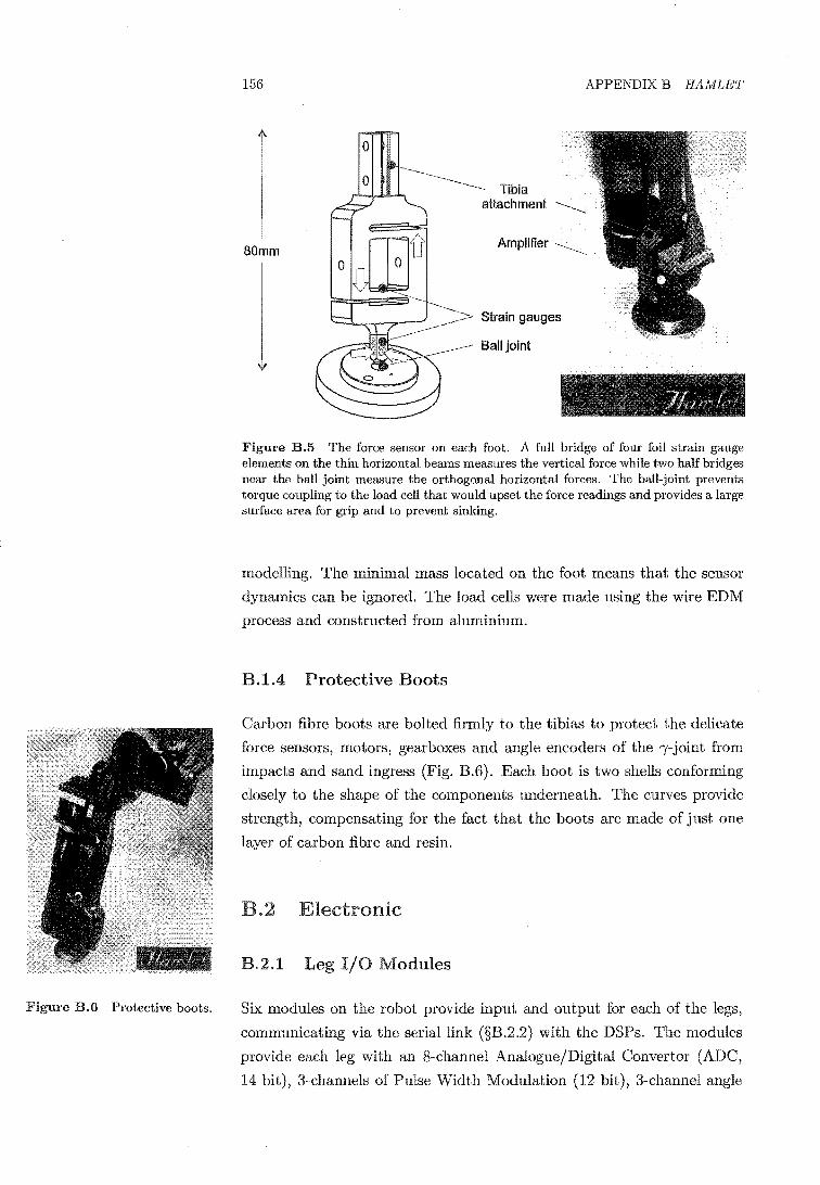
Figure B.B Protective boots.

156

80mm

v

Tibia attachment

APPENDIX B HAMLET

Amplifier ~

Strain gauges

Ball joint

Figure B.5 The force sensor on each foot. A full bridge of four foil strain gauge elements on the thin horizontal beams measures the vertical force while two half bridges near the ball joint measure the orthogonal horizontal forces. The ball-joint prevents torque coupling to the load cell that would upset the force readings and provides a large surface area for grip and to prevent sinking.

modelling. The minimal mass located on the foot means that the sensor

dynamics can be ignored. The load cells were made using the wire EDM

process and constructed from aluminium .

. 1.4 Protective Boots

Carbon fibre boots are bolted firmly to the tibias to protect the delicate

force sensors, motors, gearboxes and angle encoders of the I-joint from

impacts and sand ingress (Fig. B.6). Each boot is two shells conforming

closely to the shape of the components underneath. The curves provide

strength, compensating for the fact that the boots are made of just one

layer of carbon fibre and resin .

. 2 Electronic

B.2.1 I/O Modules

Six modules on the robot provide input and output for each of the legs,

communicating via the serial link (§B.2.2) with the DSPs. The modules

provide each leg with an 8-channel Analogue/Digital Convertor (ADC,

14 bit), 3-channels of Pulse Width Modulation (12 bit), 3-channel angle

B.2 ELECTRONIC 157

Figure B.T Hamlet's leg I/O modules and main onboard power supply. This photo shows the motor driver ICs without their heatsinks.

and velocity measurement (24 bit, by counting and encoder pulses and

measuring their period) and some digital I/O. Each module uses a Xilinx

Field-Programmable Gate Array (FPGA) so that the design can be up­

dated as needed, and has onboard linear power supplies to minimize ADC

noise.

Fig. B.7 shows the six modules fixed to the chassis. Data progresses

through the modules in a chain starting at the top right in Fig. B.7, and

ending top left. The switched mode power supply module at the very top

of the photograph converts 18VDC from the external power supply to the

variety of voltages required by the modules.

The DSPs program a divider in the first module with the sample rate

(200Hz for all the experiments carried out so far) and that module trig­

gers the remaining modules to ensure that they sample simultaneously.

Sampling and PWM stop if no data returns from the DSPs, providing a

failsafe in the event of a software crash.

B.2.2 Serial Link

The custom designed serial link transfers data between the I/O modules

on the robot and also to and from the DSPs. The link is asynchronous, full

duplex at 4 Mbit/s and uses RS-485 over twisted pair for noise immunity.

Each word has 24 bits, one start bit to align the receiver with the incoming

Daisy chain

158 APPENDIX B HAMLET

102 words ~---7

Figure B.B Hamlet's Serial link protocol and timing.

data and approximately two stop bits after the last bit (Fig. B.8).

The serial link design allows many heterogeneous modules to coexist, all

cooperating to send and receive their data sequentially through one trans­

mit and one receive channel. After the first I/O module receives its data

from the DSPs (it always gets the same number of data words) it passes

any overflowing data unchanged onto the next module. Each module op­

erates the same way until all the modules have received their updated

data. When the sender stops transmitting for a relatively long time (i.e.

between samples) the modules reset and wait for the next burst of data.

To transmit from the robot to the DSPs, the modules use the line re:­

ceiving data from the next module in the chain to control that module,

preventing it from transmitting until a suitable time. The first module

in the chain sends its data as soon as it receives the sample signal, but

meanwhile prevents the second module from transmitting. When the first

module finishes it allows the second to send; the first module passes the

second module's data through unchanged. This process continues until

after the last module sends its data at which time the line is idle for some

time and all the modules reset.

Base Electronics

As described in §3.2.2, two Texas Instruments TMS320C44 DSPs sited

on an LSI QPC/C40s carrier board (Loughborough Sound Images pIc,

1995b,a) run the realtime component of Hamlet's control software. An

"Odo" interface boardl equipped with a Xilinx FPGA transfers data be-

B.3 SOFTWARE 159

Robot Parallel port bus General bus

Figure B.9 Hamlet's DSP configuration showing memory spaces and communication channels.

tween the serial link and the 32 bit DSP parallel ports (Fig. B.9). Both

boards are located on the ISA bus of a Pentium computer. The SK of

Dual-Port RAM (DPRAM) provides communication between the DSPs

and the PC software (see below), while communication between the DSPs

is across an additional parallel port routed through the carrier board.

Software

Functions

The robot software running on the DSPs provides six different operating

modes with different capabilities. The modes are mutually exclusive:

This mode maintains all desired joint angles but they cannot be

Odo was designed within the Department and has been used for many other projects.

Modes

Commands

160 APPENDIX B HAMLET

changed.

Manual Recovery This mode allows the user to move individual joints

using the joystick. It is useful when the robot falls or is knocked over

when the power is off because the legs can easily be moved through

singulari ties.

Cartesian In this mode the joystick incrementally moves individual feet

in xyz, or moves the whole body by moving all the feet together.

Yaw, pitch and roll can also be adjusted.

Walking The restrictedness gait controller operates in this mode.

Compliance This mode is exactly like Cartesian mode except that the

force compliance control is active. Other software (HAMdatafind,

see below) can change the compliance online.

Dance This mode repeats a short looped sequence of body positions in

Cartesian mode, which is sometimes useful for demonstrations.

In addition to operating in different modes, the software can execute com­

mands that complete in a short period of time and return a result. Many

commands can be applied either to individual legs or to the whole robot,

and some can only be executed in certain modes:

Start/Stop Sampling Initializes the Leg Modules (§B.2.1) to start or

stop sampling.

Calibrate Joints & FLC Runs an automatic leg calibration cycle,

moving the joints slowly until they reach their known datums then

zeroing the force sensor (FLC) with the foot held in the air. Running

this command on the Body calibrates each leg in sequence.

Calibrate & FLC Zeroes the force sensor at any position. When the

Body is selected, the legs lift off the ground in two sets and first one

then the other is calibrated.

Activate/Deactivate PWM These commands turn the motors on or

off and reset the desired position to the current position so that the

legs do not suddenly move.

Move To Home Moves the foot or feet quickly to Xhome'

Ground Leg Moves the foot to X home then lowers it until the leg be­

comes overrestricted or the foot touches the ground. Executing this

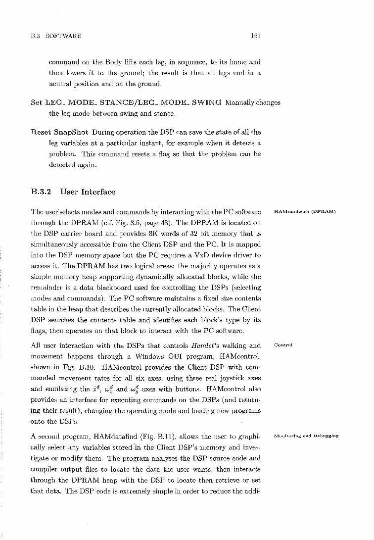
B.3 SOFTWARE 161

command on the Body lifts each leg, in sequence, to its home and

then lowers it to the ground; the result is that all legs end in a

neutral position and on the ground.

Set LEG_ L'V' ....... LJ_ STANCE!LEG_ MODE_ SWING Manually changes

the leg mode between swing and stance.

Reset SnapShot During operation the DSP can save the state of all the

leg variables at a particular instant, for example when it detects a

problem. This command resets a flag so that the problem can be

detected again.

B.3.2 User Interface

The user selects modes and commands by interacting with the PC software

through the DPRAM (c.f. 8.6, page 48). The DPRAM is located on

the DSP carrier board and provides 8K words of 82 bit memory that is

simultaneously accessible from the Client DSP and the PC. It is mapped

into the DSP memory space but the PC requires a VxD device driver to

access it. The DPRAM has two logical areas: the majority operates as a

simple memory heap supporting dynamically allocated blocks, while the

remainder is a data blackboard used for controlling the DSPs (selecting

modes and commands). PC software maintains a fixed size contents

table in the heap that describes the currently allocated blocks. The Client

DSP searches the contents table and identifies each block's type by its

flags, then operates on that block to interact with the PC software.

All user interaction with the DSPs that controls Hamlet's walking and

movement happens through a Windows QUI program, HAMcontrol,

shown in Fig. B.1O. HAMcontrol provides the Client DSP with com-

manded movement rates for all axes, using three real joystick axes

and emulating the zd, w~ and w~ axes with buttons. HAMcontrol also

provides an interface for executing commands on the DSPs (and return­

ing their result), changing the operating mode and loading new programs

onto the DSPs.

A second program, HAMdatafind (Fig. B.ll), allows the user to graphi­

cally select any variables stored in the Client DSP's memory and inves­

tigate or modify them. The program analyses the DSP source code and

compiler output files to locate the data the user wants, then interacts

through the DPRAM heap with the DSP to locate then retrieve or set

that data. The DSP code is extremely simple in order to reduce the addi-

HAMsandwlch (DPRAM)

Control

Monitoring and Debugging

Event Logging

162 APPENDIX B HAMLET

Figure B.10 HAMcontrol allows the user to send instructions for execution by the robot, including the desired walking movement.

tional processor load. Data can be continuously graphed in realtime, then

exported to Matlab or copied into other programs as an image. Variables

can also be viewed in tables and updated with new user-specified values,

they can be saved and loaded to and from disk, and there are a variety of

options for saving configurations for later reuse.

HAMviewer and HAM logger show text debugging and event messages

sent from the Client DSP. The text messages can contain data in floating

point or integer format, as well as a priority and source (what part of the

program they emanate from). HAMviewer and HAMlogger rely on a third

program, HAMmessageserver, that reads messages from the DPRAM and

acts as a Dynamic Data Exchange (DDE) server2. HAMviewer (Fig. B.12)

Figure B.ll HAMdatafind graphs and edits data on the robot.

B.3 SOFTWARE 163

·20 nsp _Subsyslem Legs inilioused: j(jnematics. PID. Camptionce. Mode Seledion 0.003 ·20 DSP _Subsystem Master s.!ling, ir~ialis.d: PID. ComPianee 0.004 ·20 DSP _Sub,ystem HAPPE Link lnili.r"ed: DMA setlings, Interrupt 3.285 DSP_Subsystem Starting sampling (should see confirrration shortly~ .. 3.292 2 DSP_Subsystem Sampling has (re~tarted Samples since DSP reboot = 1 3.292 ·20 DSP_Subsystem Force SensOlS Checked: no previou!: messages? "'" ok 3.293 McdeJniliaiisalion Inaiaflsing Cartesi3l) Mode

Figure B.12 HAMviewer, a simple program for immediately displaying selected mes­sages from the RT software.

·15 15 LeQ..Restrictedoe" 15 LeQ..ModeJnfo_M .. ·5 LeQ..Mode_Swing ·5 LeQ..Mode_cnanges ·5 LeQ..ModeJnfo_Ma, -5 LeQ..ModeJnfo_P", ·5 LeILModeJnlo_Po. ·5 LeQ..ModeJnlo_Pos ·25 LOQ..Mode_Swing 25 LeQ..RewictedJ\os. 25 LeQ..ModeJn(o_Ma, ·25 LeQ..Mode_cneng". -25 LeQ..Mode_tnlo_Ma, ·25 ·25 ·25 L"!LMtldeJnfo_P", 25 L~RefbicteldnesS'

Largest componerJ is DistanceFromHome @RJ<=-l Legit] is dangefou,iY restricted! IR,·l) Largest component is DidanceFromHome @AII ... 1 Leg(4)j, dangefou~y restricled! (R><-l) Larg .. 1 component is DislanceFromHome@ R, • 0.999 Legi2j.> LEG_MODE_EXTEND (YPrime·O.0430) Leg!2j.> LEG_MODE_STANCE (contacted 9<oun,1. R,· 0.393) Largesl component is D~lanceFromHome @A,·0.393 p,i·O,OOOO PPrime_dY.110437 2-0.0037 Body". Xc· ·1127335 Yc' ·0,20947 Leg[Oj·> LEG_MODE_EXTEND (YPrim .. O.l059) Legl5] is dar,gereu,ly restricted! (l1:<=1) L~fgest component is- Di1taocE'FlomHome@Ax=O.991 loglOj.) LEG_MODE_STANCE (contacted grOlA'ld, R, -1>.43) L"'!lO'1 component i, DWanceFI.mHome@R,-6,43 p,i = 0.0000 PPrime_dY -111220 2, {lOS50 Body".Xc. ·1126SB3 Yc' 0,37517 Legl51 i, nol dangelO'''!;> r8<IIicied anymore (A,.l)

Figure B.13 HAMlogger, a program for logging messages from the RT software and reviewing them.

shows a limited number of messages sent by the DSP in a realtime

scrolling window, filtering them by their source and priority. HAMlog­

ger (Fig. B.13) filters in the same way as HAMviewer, but HAMlogger

is slower because it retains all the messages in memory for later analysis.

Logs can also be saved and loaded from disk for permanent archiving.

The use of the DDE server means that any number of HAMviewer and

HAMlogger windows can be opened simultaneously.

2DDE is a Microsoft Windows service that allows programs to transfer data between them.

Walking Algorithm Parameters

This Appendix has tables of parameters used for the experimental work

with the robot Hamlet.

C.l Restrictedness Parameter Specification

The following list gives values for the parameters specifying the restrict­

edness components used on Hamlet. Table. 4.1 has descriptions for the

symbolic names.

RXCr) 1'-joint limit l' E [-1.048 2.590]; E = 0.1 Measured from the

femur axis (which joins the (3 and l' joints), with positive angles

being flexion of the tibia (i.e. bringing it towards the body).

RX(,B) ,B-joint limit (3 E [-0.9562.458]; E 0.02 Measured from hor­

izontal, with positive angle being depression of the femur.

RX(a) - a-joint limit Table. C.1 lists the limits of the a-joint, which

are different for each leg; E = 0.2. Angles are measured from the

robot x-axis (lateral axis) and positive angles are counterclockwise.

RX(r) - outer workspace limit Ymax O.lm, X max = 0.209m, E is the

entire region size, i.e. E = 0.1 in the Y direction and 0.209 in the x

direction.

166 APPENDIX C WALKING ALGORITHM PARAMETERS

Table C.l a-joint soft\vare limits

max 1 -1.37 0.39 2 -0.96 .87 3 -0.92 1.33 4 -0.92 1.33 5 -0,98 1.06 6 -1.37 0,58

RX(s) avoid a-axis singularity Minimum distance from the foot to

a axis 0,04m, t 0.05.

RX(a.) and RX(p.) - anterior and posterior neighbours Minimum sep­

aration of adjacent feet 0.085m 1, t = 0.04.

RX(a.f.) and RX(P.f.) anterior and posterior femurs Minimum sep­

aration of adjacent femurs 0.09m2, t 0.05.

C.2 Compliance Gains

Table C.2 Maximum active compliance gains used on Hamlet (mm/N). Values are the diagonal elements of Kac. Off-diagonal elements are zero.

y Z

0.5 2.0

0,1 2.0

lIn fact the real minimum separation is much less than this, but the simple model works on the centres of the feet and does not allow for their shape.

2See previous footnote.

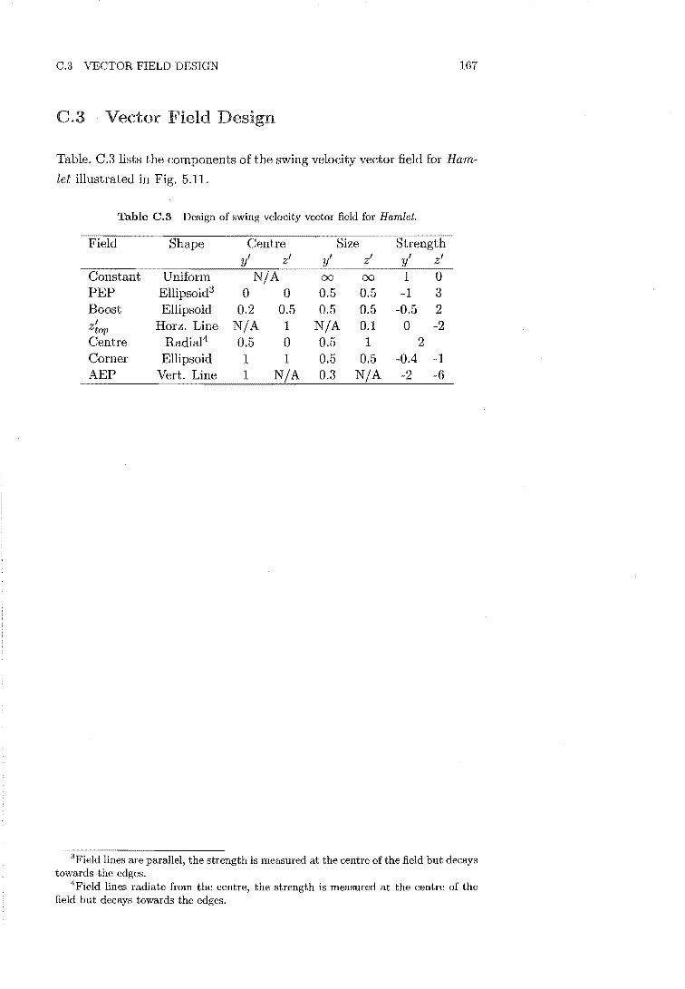
C.3 VECTOR FIELD DESIGN 167

Vector Field

Table. C.3 lists the components of the swing velocity vector field for Ham-

let illustrated in Fig. 5.11.

Table C.3 Design of swing velocity vector field for Hamlet.

Field Shape Centre Size Strength y' z' y' z' y' z'

Constant Uniform N/A 00 00 1 0 PEP Ellipsoid3 0 0 0.5 0.5 -1 3 Boost Ellipsoid 0.2 0.5 0.5 0.5 -0.5 2 ,

Horz. Line N/A 1 N/A 0.1 0 -2 Ztop

Centre Radia14 0.5 0 0.5 1 2 Corner Ellipsoid 1 1 0.5 0.5 -0.4 -1 AEP Vert. Line 1 N/A 0.3 N/A -2 -6

3Field lines are parallel, the strength is measured at the centre of the field but decays towards the edges.

4Field lines radiate from the centre, the strength is measured at the centre of the field but decays towards the edges.

APPENDIX

Miscellaneous

D.1 Swing Restrictedness Prediction

Taking the equation for an exponential:

R';redicted,swing

In R';redicted,swing (D.l)

The curve can be defined by two points: at the AEP, y* = 1 and

R;redicted,swing = R~EPl and at some point Y~odel R;redicted,swing

R~ode'

InR~EP

and InR~ode

Subtracting (D.3) from (D.2):

InR~EP -InR~ode

In R~EP R;;ode

k =

Rearranging (D.2):

In

k(l YFtx=l)

k(Y~ode - YFtx=l)

k(l YRx=l) - k(Y~ode - YRx=l)

k(l - Y~ode)

In

1 ,.

Ynode

(D.2)

(D.3)

(DA)

170 APPENDIX D MISCELLANEOUS EQUATIONS

(D.5)

.2 Ideal stance trajectory

From (5.8) we have:

(D.6)

Using only the terms from the task controller and assuming the others . d .d 'd T' d T are zero, X body = [x Y 0] and nbody [0 0 wz ] :

[ x (t) ] [ xd

(t)] [0 -wd 0 ][ x(t) ] z

y (t) - yd (t) - w~ 0 0 y (t) (D.7)

Z (t) o 0 0 0 z (t)

The movements in x and y become:

x (t) = + y (t)w~ (D.8)

y (t) ·d x (t)w; (D.9) - -y

Differentiating (D.9) and substituting (D.8) into it, and vice versa:

x (t)

ii (t)

w~ (_yd - x (t) w~)

-w~ii x (t) w~2 -w~ (_±d + y (t) w~)

w;±d - y (t) W~2

(D.lO)

(D.ll)

(D.10) and (D.ll) are second order differential equations and could be

solved. The particular solutions could be found by using x(O) Xhome

and y(O) = Yhomel and (D.8) and (D.9) at t 0 as well.

APPENDIX

Additional Modelling Results

This appendix contains additional results of simulations undertaken to

optimize the Basic 3 Legged Restrictedness Model (Chapter 6).

172 APPENDIX E ADDITIONAL MODELLING RESULTS

a) b) 100 100

75 75

~ 'ffi .s Q '5 '5 e: 50 e 50

"0 "0 0 0 0 0 0) 0)

25 25

0 0 0.3 0.45 0.6 0.75 0.9 0.1 0,5

fmax ll. fmax I fmax

c) d) 100

75

'ffi J .§ '5 '5 ~ 50 ~ 50 "0 "0 0 0 0 0 0) 0)

25 25

0 ° 0.001 0,2 0.4 0,1 0.5

°leel,min ll. 0reel,mln I 0reel.mln

e) f) 100 100

75 75

~ 19 .s .s '5 '5 ~ 50 ~ 50

"0 "0 0 0 0 0 0) 0)

25

° 0,5 1.5 2 0,5 0,75 0,95

IsiBP,max R~m

E.l Influence of individual B3LRM model parameters on proportion of good parameter sets for (3 = .5. Bars show the proportion of good parameter sets on the ordinate for the different values of the parameter that were simulated on the abscissa.

173

a) b) 100 100

75 75

]i ~ E E 0 0 ~ 50 C 50

"0 "0 0 0 0 0 Ol Ol

25 25

0 0 0.3 0.45 0.6 0.75 0.9 0.1 0.5

f a fmax ' fmax max

0) d) 100 100

75 75

~ 'ffi £i

0 0 C 50

~ 50

" " 0 0 0 0 Ol Ol

25 25

0 0 0.001 0.2 0.4 0.1 0.5

li.eetlmin a /ileat,mln ' 0leet,mln

e) I) 100 100

75 75

'iii = £i ~ 0 0 ';§!. 50 ~ 50 ~ ~ '0 '0 0 0 0 0 Ol Ol

25

0 0.5 1.5 2 0.5 0.75 0.95

Istep,max R~m

Figure E.2 Influence of individual B3LRM model parameters on proportion of good parameter sets for ,B = .95.

174 APPENDIX E ADDITIONAL MODELLING RESULTS

a) b)

§ © § 8

I B § 0

0.8

I 0.8

~ 0.6 0.6 j Ol Ol

c: c:

~ ~ 0.4 8 0.4 I ~

0 § ~ 0.2' 0.2 8 ~

0

8 0 11)

0.8 0 0.2 0.4 0.6 0.8 1

rmax 1!. rmax I rmax

c) d)

I ; i ;

o. 0 0.8 I I 0

0.6 § 0.6 I I Ol Ol c: c

~ 0 .~

0.4 0 0.4 ~ 0 8 8 0.2 0 0.2 0 8 ;

0 0 0 0.1 0.2 0.3 0.4 0 0.2

°lanl,min 1!. 0leel,min IOleel,min

e) f) ©

o. o. I o. o. Ol en c c .~ ~

O. o. ! ~ m o. 8 8 8 o. §

0 {';l {';l

0.5 1.5 2 0.5 0.6 0.7 0.8 0.9

'slep,max R~m

Figure E.3 Optimal parameter values for B3LRM for fJ ,5. Higher circles are more optimal, having fewer steps and fewer timesteps where the legs are restricted.

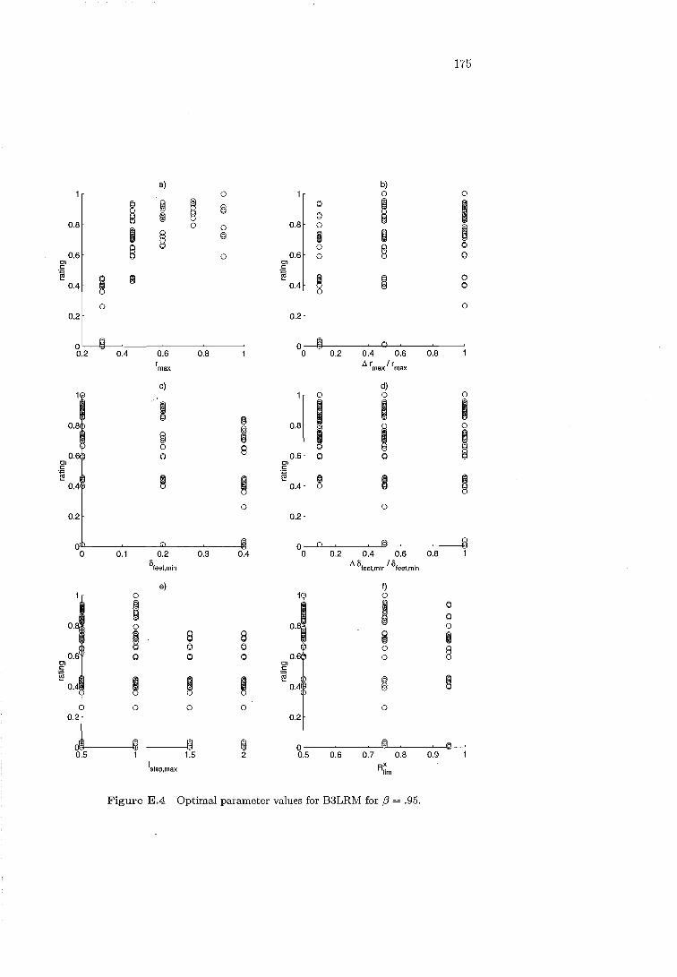
175

a) b) 0 0 0

~ ~ ; 8 0

~ I II!J 0 0.8 0 0 0.8 0

~ I ~ § i i § 0 § 0

0.6 0 0.6 0 0 OJ OJ C c

'e ~ ~ e ~ ~

0 0.4 0.4 0

0

0 0

0.2 0.2

0 0 0.2 0.4 0.6 0.8 0 0.2 0.4 0.6 0.8

r Llr / r max max max

c) d) 0 0 0

I ~ I I I o. ; 0.8

! 0

~ ! 0 8 o. 0 0.6 0 0 OJ OJ c: c: e ~ ~

'e iii ! ~ 0.4 0.4 0

0 0 0.2 0.2

0 0 0 0.1 0.2 0.3 0.4 0 0.2 0.4 0.6 0.8

°leet,min Ll 0leet,min / 0leet,min

e) f) 0 0

I I 0 0

O. 0 0

~ 8 8 iii I 0 0 0 § 0 0 0 0

OJ OJ c: c: e

~ ~ ~ .~

~ ~ o. o.

0 0 0 0 0.2 0.2

0 0.5 1.5 2 0.5 0.6 0.7 0.8 0.9

Istep,max R~m

Figure E.4 Optimal parameter values for B3LRM for {3 = .95.

References

Akay, Bassler, U., Gerharz, and Buschges, A., (2001). The role

of sensory signals from the insect coxa-trochanteral joint in controlling

motor activity of the femur-tibia joint. Journal of Neurophysiology,

85(2), p 594-604.

Alexandre, P. and Preumont, A., (1996). On the gait control of a six­

legged walking machine. International Journal of Systems Science,

27(8), p 713-721.

Altman, J. S. and Kien, J., (1985). The anatomical basis for Int·ers·eg­

mental and bilateral coordination in locusts. In Bush, B. M. and

Clarac, F., editors, Coordination of motor behaviour, 24 of Society for

Experimental Biology Seminar Series, p 91-120. Cambridge University

Cambridge, UK.

Bares, J. E. and Wettergreen, D., (1999). Dante II: Technical description,

results, and lessons learned. International Journal of Robotics Research,

18(7), p 621-649.

Barnes, D., (1988). Hexapodal robot locomotion over uneven terrain. In

Proc. IEEE Conference on Control Applications (CCA '98), 1, P

Trieste, Italy.

Bartling, C. and Schmitz, J., (2000). Reaction to Distrubances of a Walk-

ing During Stance. Journal of Experimental Biology, 203, p 1211-

1223.

Bassler, U.) ( 1977 a). Sense organs in the femur of the stick insect and their

relevance to the control of position of the femur-tibia joint. Journal of

Comparative Physiology, 121, p 99-113.

Bassler, U., (1977b). Sensory Control of Movement in the Stick Insect

Carausius Morosus. Biological Cybernetics, p 61-72.

178 REFERENCES

Beer, R D., Quinn, RD., Chiel, H. J., and Ritzmann) R E., (1997).

Biologically inspired approaches to robotics. Communications of the

Acm, 40(3), p 31-38.

Berns, K., Dillmann, R, and Piekenbrock, S., (1995). Neural Networks for

the Control of a 6-Legged Walking Machine. Robotics and Autonomous

Systems, 14(2-3), p 2:33-244.

Bowerman, R F., (1981). Arachnid Locomotion. In Herried, Clyde F.) I.

and Fourtner, C. R, editors, Locomotion and Energetics in Arthropods,

p 73-102. Plenum Press, New York.

Brooks, R A., (1986). A Robust Layered Control System For A Mobile

Robot. International Journal of Robotics and Automation, 2(1), p

14-23.

Brooks, R A., (1989). A Robot That Walks; Emergent Behaviors from a

Carefully Evolved Network. Neural Computation, 1, p 253-262.

Celaya, E. and Porta, J. M., (1996). Control of a Six-Legged Robot

Walking on Abrupt Terrain. In Froc. IEEE International Conference

on Robotics and Automation (ICRA '96) , p 2731-2736.

Chapman, R. (1998). The Insects: Structure and Function. Cambridge

University Press, Cambridge, UK, 4th edition.

Chen, C. H., Kumar, V., and Luo, Y. C., (1999). Motion planning of

walking robots in environments with uncertainty. Journal of Robotic

Systems, 16(10), p 527-545.

Chen, W., Yeo, S. H., and Low, K. H., (1997). Modular Formulation

of Dynamics of Multi-Legged Robots. In Froc. IEEE International

Conference on Robotics and Automation (ICRA '97), p 279-284.

Collins, J. and Stewart, I., (1994). The Mathematical Springs in Insect

Steps. New Scientist, p 36-40.

Collins, J. J. and Stewart, 1., (1993). Hexapodal gaits and coupled non­

linear oscillator models. Biological Cybernetics) 68, p 287-298.

Conrad, J. M. and Mills, J. W., (1998). Stiquito: advanced experiments

with a simple and inexpensive robot. IEEE Computer Society Press,

Los Alamitos, CA, USA.

Cruse, H., (1976a). The control of body position in the stick insect Ca­

rausius morosus, when walking over uneven surfaces. Biological Cyber­

netics, 24, p 25-33.

REFERENCES 179

Cruse, (1976b). The Function ofthe Legs in the Free Walking Insect,

Carausius morosus. Journal of Comparative Physiology, 112(2), p 235~

262.

Cruse, (1979), The Control of the Anterior Extreme Position of the

Hindleg of a Walking Stick Insect, Carausius Morosus. Physiological

Entomology, p 121~124,

Cruse, (1985), Co activating influences between neighbouring legs in

walking insects. Journal of Experimental Biology, 114, p 513-519,

Cruse, H., (1990), What Mechanisms Coordinate Leg Movement in Walk­

ing Arthropods? Trends in Ne'uTOscience, 13, p 15~20.

Cruse, H. and Bartling, C., (1995). Movement of Joint Angles in the Legs

of a Walking Carausius Morosus. Journal of Insect Physiology,

41(9), p 761~771.

Cruse, H" Kindermann, T., Schumm, M., Dean, J., and Schmitz, J.,

(1998). vValknet a Biologically Inspired Network to Control Six-Legged

Walking. Neural Networks, 11, p 14351447.

Cruse, H., Schmitz, J., Braun, V., and Schweins, A., (1993). Control

of Body Height in a Stick Insect Walking on a Treadmill. Journal of

Experimental Biology, 181, p 141~155.

Cruse, H. and Schwarze, (1988). Mechanisms of coupling between

the ipsilateral of a walking insect (Carausius morosus). Journal of

Experimental Biology, 138, p 455-469.

Cymbalyuk, G. S., Borisyuk, R. M., Mueller-Wilm, V., and Cruse, H.,

(1998). Oscillatory network controlling six-legged locomotion. Opti­

mization of model parameters. Neural Networks, 11(7-8), p 1449-1460.

Dean, J., (1991a). A model of leg coordination in the stick insect, Ca­

rausius morosus: I: A geometrical consideration of contralateral and

ipsilateral coordination mechanisms between two adjacent legs. Biolog-

ical Cybernetics, p 393-402.

Dean, J., (1991b). A model of coordination in the stick insect, Carau-

sins morosus: II: Description the kinematic model and simulation of

normal step patterns. Biological Cybernetics, p 403-411.

Dean, J., Kindermann, Schmitz, J., Schumm, M' l and Cruse, H.,

(1999), Control of walking in the stick insect: From behavior and

physiology to modeling. Autonomous Robots, 7(3), P 271-288.

180 REFERENCES

Dean, J. and Wendler, G., (1982). Stick insects walking on a wheel:

Perturbations induced by obstruction of leg protraction. Jo'urnal of

Comparat'tve Physiology, 148, p 195-207.

Dean, J. and '\Tendler, G., (198a). Stick Insect Locomotion on a Walking

Wheel: Interleg Coordination of

Biology, 103, p 75-94.

Position. Journal of Experimental

Dean, J. and Wendler, G., (1984). Stick insects walking on a wheel:

Patterns of stopping and starting. Journal of Experimental Biology,

110, p 20a-216.

Delcomyn, F., (1981). Insect Locomotion on Land. In Herried, Clyde F., 1.

and Fourtner, C. R, editors, Locomotion and Energetics in Arthropods,

p 103-125. Plenum Press, New York.

Delcomyn, F., (1985). Factors Regulating Insect Walking. Annual Review

of Entomology, 30, p 2a9-256.

Delcomyn, F., (1999). Walking robots and the central and peripheral

control of locomotion in insects. Autonomous Robots, 7(3), p 259-270.

Delcomyn, F. and Nelson, M. E., (2000). Architectures for a biomimetic

hexapod robot. Robotics and Autonomous Systems, 30(1-2), p 5-15.

Delcomyn, F., Nelson, M. E., and Cocatre-Zilgien, J. H., (1996). Sense

Organs of Insect Legs and the Selection of Sensors for Agile Walking

Robots. International Journal of Robotics Research, 15(2), p 113-127.

Dunlop, G. R, Cree, A. G., Katzir, S., and Yang, J. L. C., (1999). Machine

control with real time Linux. In Proceedings on Control, 32, p 1-6,

Auckland, NZ.

Duysens, J., Clarac, and Cruse, H., (2000). Load-regulating mecha-

nisms in gait and posture: Comparative aspects. Physiolog'ical Reviews,

80(1), p 83-133.

Engeln-Miillges, G. and Uhlig, F., (1996). Numerical Algorithms with C.

Springer, Berlin.

Epstein, S. and Graham, D., (198a). Behavior and motor output for an

insect walking on a slippery surface. 1. Forward walking. Journal of

Experimental Biology, 105, p 215-229.

Espenschied, K. S., Quinn, R D., Beer, R D., and Chiel, H. J., (1996).

Biologically based distributed control and local reflexes improve rough

REFERENCES 181

terrain locomotion in a hexapod robot. Robotics and Autonomous Sys­

tems, 18, p 59-64.

Field, L. H., (1978). The Stridulatory Apparatus of New Zealand Wetas in

the Genus Hemideina (Insecta: Orthoptera: Stenopelmatidae). Journal

of the Royal Society of New Zealand, 8(4), p 359-375.

Fielding, M. R and Dunlop, R, (2001). Exponential Fields to Establish

Inter-leg Influences for Omnidirectional Hexapod Gait. In Proc. 4th

International Conference on Climbing and Walking Robots (CLAWAR

2001),4, p 587-594, Karlsruhe, Germany.

Fielding, M. R, Dunlop, R, and Damaren, C. J., (2001). Hamlet:

Force/Position Controlled Hexapod Walker - Design and Systems. In

Proc. IEEE Conference on Control Applications (CCA 2001), p 984-

989, Mexico City, Mexico.

Fischer, H., Schmidt, J., R, and Buschges, A., (2001). Pattern

generation for walking and searching movements of a stick insect leg. 1.

Coordination of motor activity. Journal of Neurophysiology, 85(1), p

341-353.

Foth, E. and Bassler, U., (1985). Leg movements of stick insects walking

with five legs on a treadwheel and with one leg on a motor-driven belt.

1. General results and 1:1 coordination. Biological Cybernetics, 51, p

313-318.

Frantsevich, L. 1., (1997). Artifactual Motility of the Subcoxal Axis in a

Model Insect Leg with Skew Joint

184, p 271-277.

Journal of Theoretical Biology,

Gardner, J. F., (1991). Characteristics and Approximations of Optimal

Force Distributions in Walking Machines on Rough Terrain. In Proc.

IEEE International Conference on Advanced Robotics (ICAR '91), p

613-618.

Gorinevsky, D. M. and Shneider, A. (1990). Force Control in Loco-

motion of Legged Vehicles over Rigid and Soft Surfaces. International

Journal of Robotics Research, 9(2), p 4-23.

Graham, D., (1972). A Behavioural Analysis of the Temporal Organi­

sation of Walking Movements in the 1st Instal' and Adult Stick Insect

(Carausius morosus). Journal of Compamtive Physiology, 81, p 23-52.

182 REFERENCES

Graham, D., (1977). The effect of amputation and leg restraint on the free

walking coordination of the stick insect Carausius morosus. Journal of

Comparative Physiology, 116, p 91-116.

Graham, D., (1978). Dnusual step patterns in the free walking grasshop­

per Neoconocephalus robustus. 1. General features of the step pattern.

Journal of Experimental Biology, 73, p 147-157.

Graham, D., (1985). Pattern and Control of Walking in Insects. Advances

in Insect Physiology, 18, p 31-140.

Graham, D. and Bassler, D., (1981). Effects of afference sign reversal on

motor activity in walking stick insects (Carausius morosus). Journal of

Experimental Biology, 91, p 179-193.

Grand, C., BenAmar, F., Bidaud, P., and Andrade, G., (2001). Simulation

System for the Behaviour Evaluation of Off-road Rover. In Proc. 4th

International Conference on Climbing and Walking Robots (CLAWAR

2001), p 307-314.

Hartikainen, K K, Halme, A. J., Lehtinen, and Koskinen, K 0.,

(1992). MECANT I: A Six-Legged Walking Machine for Research Pur­

poses in Outdoor Environment. In Proc. IEEE International Conference

on Robotics and Automation (ICRA '92), p 157-163.

Hughes, G. M., (1952). The coordination of insect movements. I. The

walking movements of insects. Journal of Experimental Biology, 29, p

267-284.

Hughes, G. M., (1957). The coordination.of insect movements. II. The ef­

fect of limb amputation and the cutting of commissures in the cockroach

Blatta orientalis. Journal of Experimental Biology, 34, p 306-333.

Inagaki, K and Kobayashi, H., (1994). Adaptive Wave Gait for Hexa­

pod Synchronized Walking. In Proc. IEEE International Conference on

Robotics and Automation (ICRA '94), p 1326-1331.

Ishiguro, A., Kuboshiki, S., Ichikawa, S., and Dchikawa, Y., (1996). Gait

control of hexapod walking robots using mutual-coupled immune net­

works. Advanced Robotics, 10(2), p 179-195.

Johnston, R. M. and Levine, R. B., (1996). Locomotory behavior in the

hawkmoth Manduca sexta: Kinematic and electromyographic analy­

ses of the thoracic legs in larvae and adults. J01.Lrnal of Experimental

Biology, 199(4), p 759-774.

REFERENCES 183

Kaneko, M., Tanie, K, and Than, M. N. M., (1988). A Control Algorithm

for Hexapod Walking Machine Over Soft Ground. Joumal of Robotics

and Automation, 4(3), p 294-302.

Kazerooni, H., Sheridan, T. B., and Houpt, P. K, (1986). Robust Com­

pliant Motion for Manipulators, Part I: The Fundamental Concepts of

Compliant Motion. Joumal of Robotics and Automation, 2(2), p 83-92.

Klein, C. A. and Briggs, R L., (1980). Use of Active Compliance in the

Control of Legged Vehicles. In IEEE Transactions on Systems, Man

and Cybemetics, 10, p 393-399.

Klein, C. A., Olson, K W., and Pugh, D. R, (1983). Use of Force and

Attitude Sensors for Locomotion of a Legged Vehicle over Irregular

Terrain. Intemational Joumal of Robotics Research, 2(2), p 3-17.

Koyachi, N., Arai, T., Adachi, H., Murakami, A., and Kawai, K, (1997).

Mechanical Design of Hexapods with Integrated Limb Mechanism:

MELMANTIS-1 and MELMANTIS-2. In Pmc. IEEE Intemational

Conference on Advanced Robotics (ICAR '97), p 273-278.

Krotkov, E. and Simmons, R, (1996). Perception, Planning, and Control

for Autonomous Walking With the Ambler Planetary Rover. Intema­

tional Joumal of Robotics Research, 15(2), p 155-180.

Kumar, V. R and Waldron, K J., (1989). Adaptive Gait Control for a

Walking Robot. Joumal of Robotic Systems, 6(1), p 49-76.

Land, M. F., (1972). Stepping movements made by jumping spiders during

turns mediated by the lateral eyes. Joumal of Experimental Biology,

57, p 15-40.

Lawrence, D. A. and Stoughton, R M., (1987). Position-Based Impedance

Control: Achieving Stability in Practice. In Proc. AIAA Guidance,

Navigation and Control Conference, p 221-226.

Lee, W.-J. and Orin, D. E., (1988a). The Kinematics of Motion Plan­

ning for Multilegged Vehicles Over Uneven Terrain. IEEE Joumal of

Robotics and Automation, 4(2), p 204- 212.

Lee, W.-J. and Orin, D. E., (1988b). Omnidirectional Supervisory Control

of a Multilegged Vehicle Using Periodic Gaits. IEEE Joumal of Robotics

and Automation, 4(6), p 63~642.

Loughborough Sound Images pIc., (1995a). C4x Network API Support

User's Guide. Manual, Loughborough Sound Images pIc.

184 REFERENCES

Loughborough Sound Images pIc., (1995b). QPC/C40S TIM-40 Carrier

Board Technical Reference ManuaL Manual, Loughborough Sound Im­

ages pIc.

Luk, B. L., Galt, S., and Chen, S., (2001). Using genetic algorithms to

establish efficient walking gaits for an eight-legged robot. International

Journal of Systems Science, 32(6), p 703~713.

Marhefka, D. W. and Orin, D. E., (1997). Gait Planl1ing for Energy Ef:'

ficiency in Walking Machines. In Proc. IEEE International Conference

on Robotics and Au,tomation (ICRA '97), p 474-480, Albuquerque, New

Mexico, USA.

McGhee, R. B., (1968). Some Finite State Aspects of Legged Locomotion.

Mathematical Biosciences, 2, p 67~84.

Moore, H. J. and Jakosky, B. M., (1989). Viking Landing Sites, Remote­

Sensing Observations, and Physical Properties of Martian Surface Ma­

terials. Icarus, 81(1), p 164-184.

Nagy, P. V., (1993). Modeling Walker/Terrain Interaction to Acheive

Reliable, Autonomous \Valking ControL In Proc. IEEE International

Symposium on Intelligent Control (ISIC '93), p 202-207.

Pal, P. K. and Kar, D. C., (2000). Gait optimization through search.

International Journal of Robotics Research, 19(4), p 394-408.

Pal, P. K, Mahadev, V., and Jayarajan, K., (1994). Gait Generation for

a Six-legged Walking Machine through Graph Search. In Proc. IEEE

International Conference on Robotics and Automation (ICRA '94), 2,

p 1332~1337, San Diego, USA.

Pearson, K G. and Franklin, R., (1984). Characteristics of Leg Movements

and Patterns of Coordination in Locusts Walking on Rough Terrain.

International Journal of Robotics Research, 3(2), p 101-112.

Pearson, K G. and Iles, J. F., (1973). Nervous mechanisms underlying

intersegmental co-ordination of leg movements during walking in the

cockroach. Journal of Experimental Biology, 58, p 725~744.

Pfeiffer, F., Eltze, J., and 'Weidemann, H.-J., (1995). 6-Legged Technical

Walking Considering Biological Principles. Robotics and Autonommts

Systems, 14(2-3), p 223-232.

REFERENCES 185

Pfeiffer, F., Weidemann, H.-J., and Danowski, P., (1990). Dynamics of

the Walking Stick Insect. In Proc. IEEE International Conference on

Robotics and Automation (ICRA '90), 3, p 1458-1463.

Quinn, R. D., Nelson, G. M., Bachmann, R. J., and Ritzmann, R.

(2001). Toward mission capable legged robots through biological inspi­

ration. Autonomous Robots, 11(3), p 215-220.

Roeder, K. D., (1937). The control of tonus and locomotor activity in the

praying mantis (Mantis L\JL.'i".'\JDU L.). J07.lrnal of Experimental Zoology,

76, p 353-74.

Rover Team., (1997). Characterization of the Martian Surface Deposits

by the Mars Pathfinder Rover, Sojourner. Science, 278, p 1765-1768.

Salmi, S. and Halme, A., (1996). Implementing and testing a

reasoning-based free gait algorithm in the six-legged walking machine,

"MECANT". Control Engineering Practice, 4(4), p 487-492.

Schmucker, U., Scheider, A., and Ihme, T., (1996). Six-Legged Robot for

Service Operations. In Proc. IEEE Eurobot, p 135-142.

Schneider, M. and Miiller, J., (1999). Force Based Motion Control of the

Walking Machine ALDURO Using Exact Linearization Methods. In

Proc. IEEEj ASME International Conference on Advanced Intelligent

Mechatronics, p 537-542.

Seraji, H., (1998). Nonlinear and Adaptive Control of Force and Com­

pliance in Manipulators. International Journal of Robotics Research,

17(5), p 467-484.

Shih, L., Frank, A. A., and Ravani, B., (1987). Dynamic Simulation of

Legged Machines Using a Compliant Joint Model. International Journal

of Robotics Research, 6(4), p 33-46.

Song, S.-M. and 'Waldron, K. J., (1987). An Analytical Approach for

Gait Study and Its Applications on Wave Gaits. International Journal

of Robotics Research, 6(2), p 60-71.

Spirito, C. P. and Mushrush, D. L., (1979). Interlimb coordinatin during

slow walking in the cockroach. 1. Effects of substrate alterations. Journal

of Experimental Biology, 78, p 233--243.

Takahashi, Y., Arai, T., Mae, Y., Inoue, K., and Koyach, N., (2000). De­

velopment of Multi-Limb Robot with Omnidirectional Manipulability

186 REFERENCES

and Mobility. In Proc. IEEE/RSJ International Conference on Intel­

ligent Robots and Systems (IROS '00), 3, p 2012-2017, Takamatsu,

Japan.

Waldron, K. J., (1986). Force and Motion Management in Legged Loco­

motion. Journal of Robotics and Automation, 2(4), p 214-220.

Waldron, K. J., Vohnout, V. J., Pery, A., and McGhee, R. B., (1984).

Configuration Design of the Adaptive Suspension Vehicle. International

Journal of Robotics Research, 3(2), p 3748.

Wang, J. Rong, S. N., Zhang, B. P., Guo, G., and Gruver, W. A.,

(1994). An Omnidirectional Dual Tripod Walking Machine: Mechani­

cal Structure and Control. In Proc. IEEE/RSJ/GI International Con­

ference on Intelligent Robots and Systems (IROS '94), 5, p 385~390.

Weidemann, H., Eltze, J., and Pfeiffer, F., (1993). Leg Design Based

on Biological Principles. In Proc. IEEE International Conference on

Robotics and Automation (ICRA '93), 3, p 352-358.

Weidemann, H.-J., Pfeiffer, F., and Eltze, J., (1994). The Six-Legged

TUM Walking Robot. In Proc. IEEE/RSJ/GI International Conference

on Intelligent Robots and Systems (IROS '94), 2, p 1026-1033.

Wendler, G., (1964). Laufen und Stephen der Stabheuschreke Carausius

morosus: Sinnesborstenfelder in den Beingelenken als Glieder von Re­

galkreisen. Zeitschrift fur Vergleichende Physiologie, 51, p 60-66.

Wendler, G., (1966). The coordination of walking movements in arthro­

pods. In Symposium of Society of Experimental Biologists, 20, p 229-

249.

Wendler, G., (1972). Keorperhaltung bei der Stabheuschrecke: Ihre

Beziehung zur Schwereorientierung und Mechanimen ihrer Reglung.

Verh. Dtsch. Zool. Ges., 65, p 215-219.

Wessel, P. Single and Multiple Regression,

http://www.soest.hawaiLedu/wessel/courses/gg313/DA_

book/ node88.html.

(2001).

Wettergreen, D. and Thorpe, C., (1996). Developing Planning and Reac­

tive Control for a Hexapod Robot. In Proc. IEEE International Con­

ference on Robotics and Automation (ICRA '96), p 2718.

Wilson, D. M' l (1966). Insect Walking. Anmtal Review of Entomology,

11, p 103-122.

REFERENCES 187

Wong, T. P., (1999). Use of a Delta Robot as a Walking Machine. Masters

of engineering, University of Canterbury.

J. L. C., (2000). Computer Controlled Multi-Axis robot. Masters of

engineering, University of Canterbury.

Zolotov, V., Frantsevich, L. 1., and Falk, E., (1975). Kinematik der pho­

totaktischen Drehung bil der Honigbiene Apis mellifera. Journal of

Comparative Physiology, 97, p 339-353.